this document downloaded from ... · pdf filethis document downloaded from ... theory...
TRANSCRIPT

This document downloaded from vulcanhammer.net vulcanhammer.info
Chet Aero Marine
Don’t forget to visit our companion site http://www.vulcanhammer.org
Use subject to the terms and conditions of the respective websites.

ENCE 3610ENCE 3610Soil MechanicsSoil Mechanics
Lecture 9Settlement and Consolidation of Soils

Overview
Soil is a nonhomogeneous porous material consisting of three phases Solids Fluid (normally water) Air
Soil deformation may occur by change in: Stress Water content Soil mass Temperature
When soil deformation takes place below a foundation, it results in settlement
Settlement of soils below foundations is the most common cause of foundation failure

Stages of Settlement Elastic Settlement Se:
settlement due to immediate elastic deformation before major particle rearrangement
Primary Consolidation Settlement Sc: settlement due to major particle rearrangement
Secondary Consolidation Settlement Ss: further particle rearrangement after primary settlement
Total Settlement St = Se + Sc + Ss
Other Types of Settlement Dynamic forces Expansive soil Collapsible soil
Types of Settlement

Settlement and Consolidation
Volume change in soils is not instantaneous: it takes place over time
How long it takes depends upon the type of soil and its permeability
Terms Settlement refers to the
distance the structure moves
Consolidation refers to the time it takes to move a certain distance
Soil Type Considerations Rate of consolidation
depends upon permeability of the soil
Cohesive soils are slow, use classic consolidation theory
Cohesionless soils are more rapid
Hough’s Method (ENCE 3610)
Schmertmann’s Method (ENCE 4610,) incorporates elasticity considerations

Elastic Settlement
Based on theory of elasticity
Load applied at a point or over an area on a semi-infinite half space
Can estimate both deflections and stresses
Theory of Boussinesq most commonly used; will discuss stresses later

Initial Settlement:Perloff's Method Variables
q = unit load on foundation (assuming uniform loading)
B = major dimension of foundation
I = combined influence factor
ν = Poisson’s Ratio Es = Modulus of
Elasticity of the soil
sc E
qBIS21

Variables for Perloff’s Method

Perloff Method Example
Solution (using method presented) Since method
determines settlement at corners, divide up foundations into quarters, determine settlement at corners and add using superposition

Perloff’s Method Example
Use 10’ x 10’ Foundation B = L = 10’ H = 10’ L/B = 1 H/B = 1 ν = 0.5 From table, I = 0.15
'9.020
5.0115.01044
1
2
2
sc E
qBIS

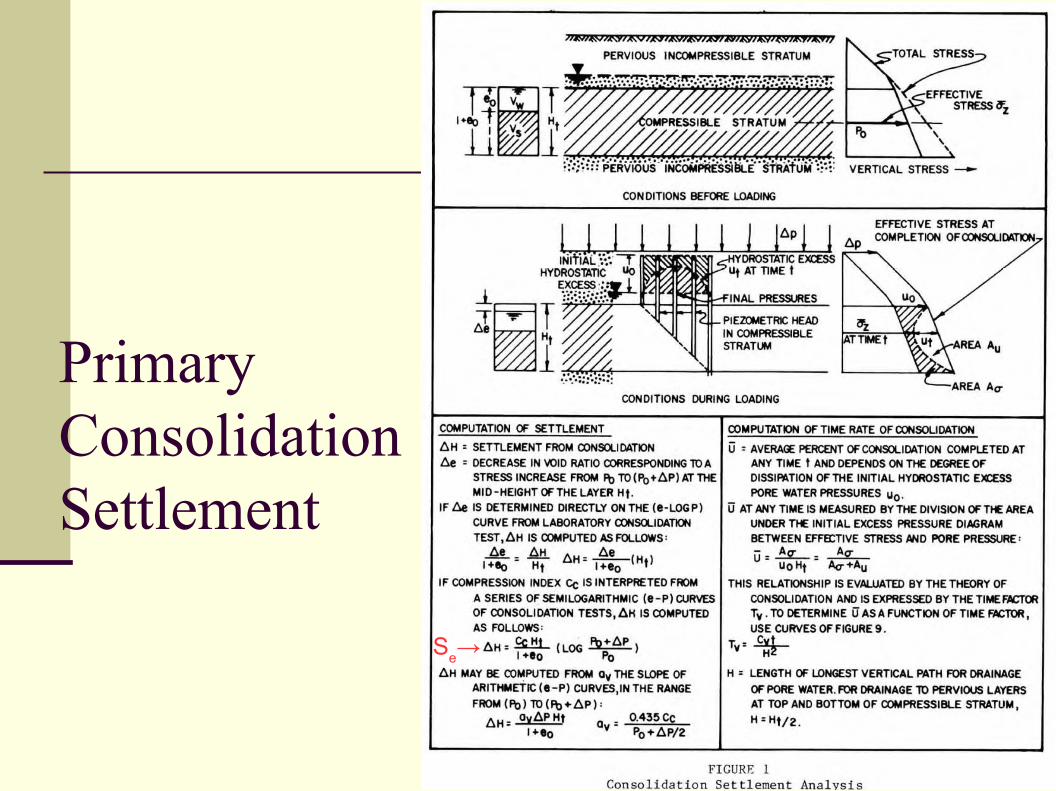
Overview of Primary Settlement and Consolidation Consolidation is the process
of gradual transfer of an applied load from the pore water to the soil structure as pore water is squeezed out of the voids.
The amount of water that escapes depends on the size of the load and compressibility of the soil.
The rate at which it escapes depends on the coefficient of permeability, thickness, and compressibility of the soil.
Two questions need to be answered by consolidation analysis: How much will the structure
settle? Generally referred to
as the “settlement” question
How long will it take for it to do so? Generally referred to
as the “consolidation” question

Principle of Consolidation

Consolidation Test
A test intended to replicate the process of primary (and secondary) settlement (distance) and time (consolidation) in the field
Necessary to run with undisturbed specimens, as disturbance changes the soil skeleton structure and thus the results

Apparatus
Consolidometer The consolidometer
has a rigid base, a consolidation ring, porous stones, a rigid loading plate, and a support for a dial indicator
Fixed or floating ring

Preparation of Specimen

Procedure
Consecutive Loads on Specimen
.5 ksf 1 ksf 2 ksf 4 ksf 8 ksf 16 ksf 32 ksf
Times to Record Data for Each Load
0.1 min 0.2 min 0.5 min 1.0 min 2.0 min 4.0 min 8.0 min 15 min
30 min
1 hr
2 hr
4 hr
8 hr
24 hr
Record the dial reading for each load increment at completion of primary consolidation for each load (usually 24 hours)
Remove load in decrements, recording dial indicator readings
Conduct a water content test on specimen after unloading is complete

Typical Results of Consolidation Tests Interpreted as a Stress-Strain Problem
The plot is semi-logarithmic with the ordinate (y-axis) logarithmic and the abscissa (x-axis) natural.
The stress-strain analogy is physically exact but does not quite correspond to theory of elasticity because the compression is not elastic (and not path independent.)
This is commonly used in the Netherlands, and is also the basis for Hough’s Method.

Typical Consolidation Results Expressed as a Function of Void Ratio
Frequently e0→
Note axes reversed
Used primarily for the consolidation of saturated clays
Primary Consolidation Settlement
Se→

Primary Compression Settlement
Strain can be defined as ε = Se/H
Primary Compression Settlement is thus more commonly written as
(normally consolidated soils) Ho = original height of
layer being compressed
eo = original void ratio
o
o
o
cc e
HCS
log1

Non-Laboratory Estimates of Compression Index
Note that “virgin” consolidation does not “kick in” until after an effective stress point is passed. The soil has been compressed to some degree by that effective stress before we add additional stress
Normally Consolidated Soils
These are used if full consolidation tests are either not possible, or for preliminary analysis

Sample Settlement Problem(Cohesive Soils) Given Two-Layer Soil Profile
Clean well-graded fine to coarse sand layer above clay layer and at surface N60 = 20 35' thick Unit weight of soil above
phreatic surface = 110 pcf Submerged weight of soil
below water table= 65 pcf Depth of water table = 15’
Clay stratum, normally consolidated LL= 45 25' thick Water Content = 40% Specific Gravity of solids
= 2.78
Given Building placed on
surface Square Foundation, 30’
x 30’ Uniform Load of 10 ksf
on entire foundation
Find Average settlement of
building due to primary settlement of clay layer
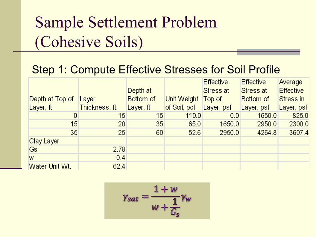
Sample Settlement Problem(Cohesive Soils)
Step 1: Compute Effective Stresses for Soil Profile

Sample Settlement Problem(Cohesive Soils) Step 2: Compute
Foundation Load for Center of Layer Depth of Center of
Layer = (15 + 20 + 25/2) = 47.5’
Step 3: Compute Compression Index and Void Ratio for Clay Layer Compression Index
Void Ratio
psf 1498
305.47
1
10000
1
2
2
=Δσ
+
=Δσ
B
z+
q=Δσ
v
v
v

Sample Settlement Problem(Cohesive Soils) Step 4: Compute Settlement Using Formula
for Cohesive Soils
"75.6
3607
14983607log
112.11
25315.012
log1
c
c
o
o
o
cc
S
S
e
HCS

Overconsolidation or Preconsolidation
☞ Overconsolidation complicates the analysis of primary settlement because the ground being compressed acts as if the previous overburden pressure is still being applied, irrespective of current overburden conditions
☞ Requires dividing the settlement analysis into two parts
☞ Sometimes referred to as preconsolidation
The ratio of the maximum overburden stress a soil has experienced to the present overburden stress
If OCR >1, the soil is overconsolidated
If OCR ~1, the soil is normally consolidated
If OCR <1, the soil is underconsolidated
cOCR

Effect on Primary Settlement
sC

Settlement in Overconsolidated Soils☞ Formula, σ’o + Δσ’ > σ’c (to the right of “F”)
☞ Formula, σ’o + Δσ’ < σ’c (to the left of “F”)
c
o
o
c
o
c
o
sc e
HC
e
HCS
log1
log1
o
o
o
sc e
HCS
log1

Overconsolidated Example☞ Given
☞ Soil with void ratio-log pressure as shown
☞ 6' thick clay layer under sand layer
☞ Two possible additional loadings:
☞ 5 tsf☞ 7.5 tsf
☞ Find☞ OCR☞ Settlement for each
case

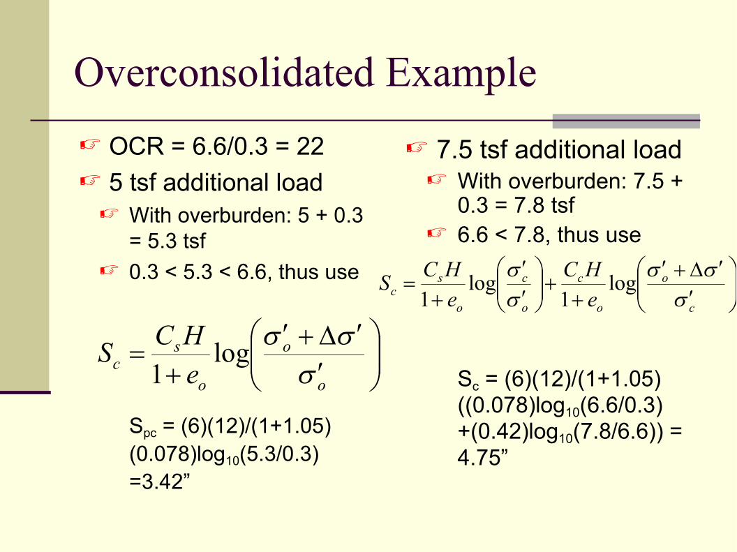
Overconsolidated Example
☞ OCR = 6.6/0.3 = 22☞ 5 tsf additional load
☞ With overburden: 5 + 0.3 = 5.3 tsf
☞ 0.3 < 5.3 < 6.6, thus use
Spc = (6)(12)/(1+1.05)(0.078)log10(5.3/0.3)=3.42”
☞ 7.5 tsf additional load☞ With overburden: 7.5 +
0.3 = 7.8 tsf☞ 6.6 < 7.8, thus use
Sc = (6)(12)/(1+1.05)((0.078)log10(6.6/0.3)+(0.42)log10(7.8/6.6)) = 4.75”
o
o
o
sc e
HCS
log1
c
o
o
c
o
c
o
sc e
HC
e
HCS
log1
log1

Multiple Layers
☞ Multiple layers can be handled by computing the single layer consolidation for each and summing the displacements
☞ Take care to properly compute or assign the additional vertical stresses generated by the surface load for each layer (not all of the stresses will be the same)
☞ Take care when dealing with overconsolidated soils to properly understand the consolidation region for each layer

Secondary Compression of Cohesive Soils
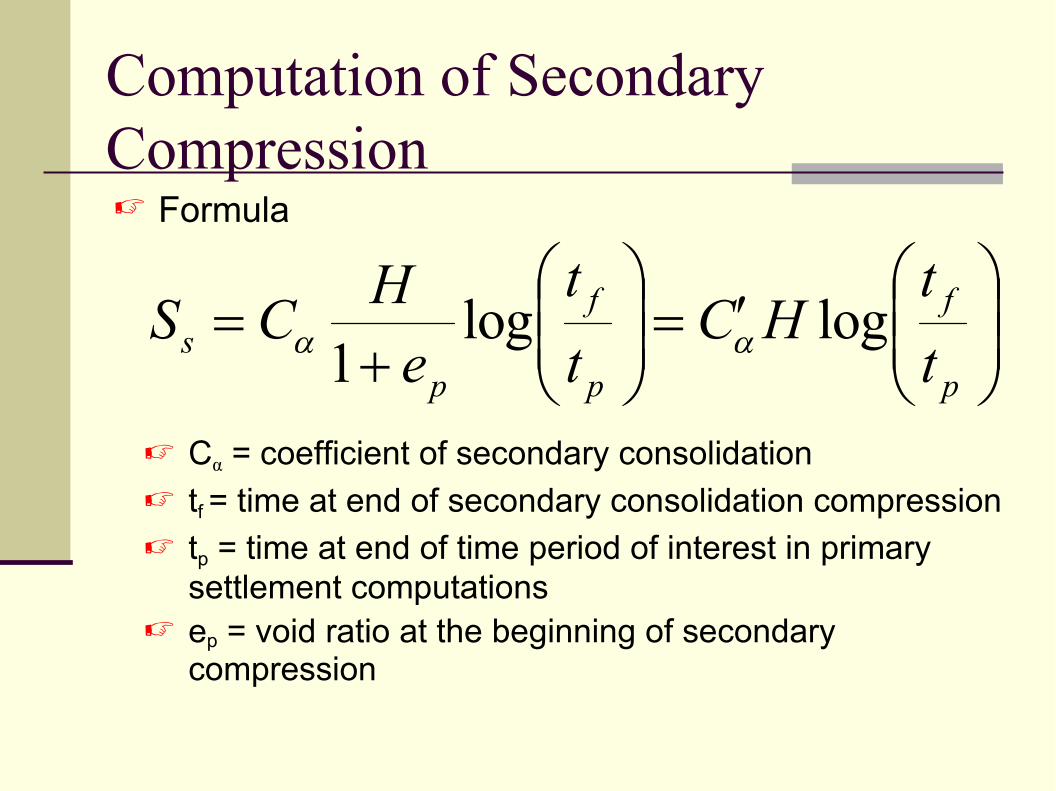
Computation of Secondary Compression☞ Formula
☞ Cα = coefficient of secondary consolidation☞ tf = time at end of secondary consolidation compression☞ tp = time at end of time period of interest in primary
settlement computations☞ ep = void ratio at the beginning of secondary
compression
p
f
p
f
ps t
tHC
t
t
eH
CS loglog1

Example of Secondary Compression
☞ Given☞ As shown☞ Primary Settlement Data
☞Expected time for primary consolidation ~ 13 years
☞eo = 1 (at beginning of primary consolidation)
☞Normally consolidated clay, Cc = 0.21
☞ Desired life of structure = 110 years
☞ Cα = 0.02
☞ Find☞Secondary
Consolidation Settlement

Secondary Compression Example
☞ Primary Compression Calculation
☞ Compute void ratio ep at end of primary consolidation
☞ Secondary Compression Calculation
Total Compression = 6.35” + 1.84” = 8.19”
"35.675.
8.75.log
11121621.0
log1
o
o
o
cc e
HCS
"84.113
110log
93.011216
02.0log1
p
f
ps t
t
eH
CS
93.075.
8.75.log21.01log
o
ocoop Ceeee

Hough’s Method for Settlement of Shallow Foundations in Cohesionless Soils
• Recommended by FHWA (and thus AASHTO, state DOT’s etc.) because studies show that it is consistent and conservative
• Described in Soils and Foundations Reference Manual, pp. 7-15 to 7-19
• Requires a “layer by layer” analysis and thus should be done with a spreadsheet

Hough’s Method
1. Subdivide subsurface soil profile into approximately 3-m (10-ft) layers based on stratigraphy to a depth of about three times the footing width.
• Make sure layers are approximately homogeneous with relation to SPT blow count, unit weight and type of soil.
• Divide layers at phreatic surface (water table)2. Correct SPT blowcounts to an (N1)60 value, using methods previously discussed.3. Determine bearing capacity index (C′) using corrected SPT blowcounts, N′,
determined in Step 2.4. Calculate the effective vertical stress, σ’o, at the midpoint of each layer and the
average bearing capacity index for that layer.5. Calculate the increase in stress at the midpoint of each layer, Δσ, using 2:1
method (for this course.)6. Calculate the settlement in each layer, Ho, under the applied load using the
following formula:
7. Sum the settlements in each layer to determine the total settlement
o
oo
C
HS
log

Bearing Capacity Index Factors for Hough Method

Note max. value
kPa) Units,(SI 2100
ksf) Units,(U.S. 2 2
60601
voN
voN
N
C
C
NCN

Sample Settlement Problem(Cohesionless Soils, Hough’s Method) Given Two-Layer Soil Profile
Clean well-graded fine to coarse sand layer above clay layer and at surface N60 = 20 35' thick Unit weight of soil above
phreatic surface = 110 pcf Submerged weight of soil
below water table= 65 pcf Depth of water table = 15’
Clay stratum, normally consolidated LL= 45 25' thick Water Content = 40% Specific Gravity of solids
= 2.78
Given Building placed on
surface Square Foundation, 30’
x 30’ Uniform Load of 10 ksf
on entire foundation
Find Average settlement of
building due to settlement of sand layer
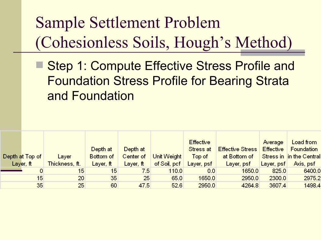
Sample Settlement Problem(Cohesionless Soils, Hough’s Method) Step 1: Compute Effective Stress Profile and
Foundation Stress Profile for Bearing Strata and Foundation

Sample Settlement Problem(Cohesionless Soils, Hough’s Method) Step 2: Correct SPT
Values for Overburden Pressure Layer 1:
(N1)60 = (1.6)(20) = 31 Layer 2: CN = 0.9,
(N1)60 = (0.9)(20) = 19
Step 3: Determine Values for C’
ksf) Units,(U.S. 2 1.56825.0
2
ksf) Units,(U.S. 2 2
60601
N
voN
N
C
C
NCN

Sample Settlement Problem(Cohesionless Soils, Hough’s Method) Step 4: Compute Settlements of Sand Layers
Layer 1:
Layer 2: S = 1.33”
"88.1825
6400825
90
'1512log
o
oo
C
HS

Time Rate of Consolidation

Overview of Time Rate Computations☞ Consolidation is a process
that takes place over time and is the result of two processes:
☞ Dissipation of excess pore water pressures created by surcharge or new foundation loads at the surface. This takes place when the excess water is drained from the soil
☞ Rearrangement of the soil particles (“soil skeleton”) to reflect new effective stress conditions created by foundation or surcharge
Assumptions Clay-water system is
homogeneous Saturation is complete Water in
incompressible Soil particles are
incompressible Flow is in one direction
only (in the direction of compression)
Darcy’s Law is valid

Consolidation ModelSign ConventionBetter Reversed

Coefficient of Compressibility
Coefficient of VolumeCompressibility
pmpe
an
ee
n
pe
a
vo
v
o
v
1
ng,Substituti
1
ipRelationshPorosity
tu
mtp
mzv
tzv
tdzdv
n
dzAtAvv
VV
n
vv
tb
T
w
ng,Substituti
u(z,t): Pressure vs. Distance and Time Variable
Continuity of Flow:

Darcy's Law
tu
mzu
k
zu
kzv
zu
kzh
kkiv
vw
w
w
2
2
2
2
1
Equating,
1
ating,Differenti
1

Consolidation Equation
☞ Rearranging,
☞ Boundary conditions are the conditions of drainage at the surfaces of the consolidating layer
☞ Initial conditions are the effective stress and pore water conditions
Coefficient of Consolidation
Key variable in primary consolidation calculations
Tends to be a constant for a given soil because the ratio of k to mv tends to remain constant
● Both of these variables tend to be directly proportional to the void ratio of the soil
2
2
2
2
zu
czu
mk
tu
vwv
vwv m
kc

Drainage Conditions
☞ Speed of the drainage depends upon the conditions at the boundaries of the drainage
☞ Drainage can be one or two ways☞ Theory based on one
way drainage☞ Distribution of initial pore
pressure can affect time rate of consolidation (see diagram at right)

Solution of Consolidation Equation
Solution Equation is a second
order, parabolic differential equation (similar to heat equation)
Solution is an infinite Fourier series with orthogonality and eigenfunctions
Solution depends upon both boundary and initial conditions
Consider the case of one way drainage
● Boundary Conditions At top of layer: p = 0
(free flow) At bottom of layer: ∂p/∂z = 0 (no flow)
● Initial Conditions p = p0 = (stress
induced by applied load, remains constant)
● Solution
2
22
412
1
1
212cos
1214 H
tci
i
i
o
v
ehz
iip
p

Time Factor for Consolidation
☞ Time Factor
☞ t = time of consolidation☞ Tv = time factor for vertical
drainage☞ Hdr = longest distance of
drainage to pervious surface☞ Usually depth of layer for
single drainage, half of layer depth for double drainage
☞ cv = coefficient of consolidation
2dr
vv H
tcT
vTi
i
i
o
ehz
iip
p 412
1
1 22
212cos
1214

Degree of Consolidation Degree of Consolidation
Expressed as a percentage Expresses ratio of both pore
pressures and settlement Allows relating settlement to
time (consolidation)
o
e
c
tc
u
u
S
SU 1
1
412
22
2
12
181
i
Ti v
ei
U

Time Factor vs. Average Degree of Consolidation
Assumes uniform initial pressure
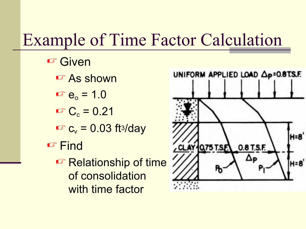
Example of Time Factor Calculation☞ Given
☞ As shown☞ eo = 1.0
☞ Cc = 0.21
☞ cv = 0.03 ft3/day
☞ Find☞ Relationship of time
of consolidation with time factor

Solution of Time Factor CalculationDays Tv
10 0 0 020 0.01 10 0.6430 0.01 10 0.6440 0.02 15 0.9550 0.02 15 0.9560 0.03 20 1.2770 0.03 20 1.2780 0.04 25 1.5990 0.04 25 1.59
100 0.05 28 1.78200 0.09 32 2.03300 0.14 40 2.54400 0.19 48 3.05500 0.23 53 3.37600 0.28 60 3.81700 0.33 63 4800 0.38 68 4.32900 0.42 72 4.57
1000 0.47 75 4.76
Hdr 8Cv 0.03Spc 6.35
Percent Consolidation
Settlement, in.
days 2130803.0
22
ttHtc
Tdr
vv
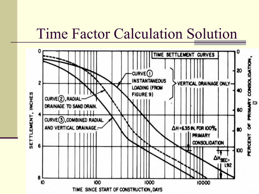
Time Factor Calculation Solution


Coefficient of Consolidation
Logarithm of Time Method
Square Root of Time Method

Accelerating Consolidation Settlement
☞ Rate of consolidation settlement under natural conditions is frequently unacceptable for actual construction and structure use
☞ Previous Example: 75% settlement @ 1000 days = 2 years 8 months 26 days
☞ Accelerating settlement if sometimes necessary to complete construction and use structure
Concept of Consolidation Acceleration Provide a high-
permeability path for the water to escape, thus reducing the time for consolidation to take place
Type of acceleration Sand Drains Prefabricated Vertical
(Wick) Drains
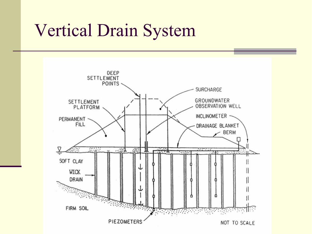
Vertical Drain System


Sand Drain Installation

Wick Drains
☞ Geosynthetic used as a substitute to sand columns; arrayed in a similar manner to the sand drains
☞ Installed by being pushed or vibrated into the ground

Installation of Wick Drains

Questions