this paper defines economic slumps as sequences of
TRANSCRIPT

econstorMake Your Publications Visible.
A Service of
zbwLeibniz-InformationszentrumWirtschaftLeibniz Information Centrefor Economics
Bluhm, Richard; de Crombrugghe, Denis; Szirmai, Adam
Working Paper
Do Weak Institutions Prolong Crises? On theIdentification, Characteristics, and Duration ofDeclines during Economic Slumps
CESifo Working Paper, No. 4594
Provided in Cooperation with:Ifo Institute – Leibniz Institute for Economic Research at the University of Munich
Suggested Citation: Bluhm, Richard; de Crombrugghe, Denis; Szirmai, Adam (2014) : Do WeakInstitutions Prolong Crises? On the Identification, Characteristics, and Duration of Declinesduring Economic Slumps, CESifo Working Paper, No. 4594, Center for Economic Studies andifo Institute (CESifo), Munich
This Version is available at:http://hdl.handle.net/10419/93438
Standard-Nutzungsbedingungen:
Die Dokumente auf EconStor dürfen zu eigenen wissenschaftlichenZwecken und zum Privatgebrauch gespeichert und kopiert werden.
Sie dürfen die Dokumente nicht für öffentliche oder kommerzielleZwecke vervielfältigen, öffentlich ausstellen, öffentlich zugänglichmachen, vertreiben oder anderweitig nutzen.
Sofern die Verfasser die Dokumente unter Open-Content-Lizenzen(insbesondere CC-Lizenzen) zur Verfügung gestellt haben sollten,gelten abweichend von diesen Nutzungsbedingungen die in der dortgenannten Lizenz gewährten Nutzungsrechte.
Terms of use:
Documents in EconStor may be saved and copied for yourpersonal and scholarly purposes.
You are not to copy documents for public or commercialpurposes, to exhibit the documents publicly, to make thempublicly available on the internet, or to distribute or otherwiseuse the documents in public.
If the documents have been made available under an OpenContent Licence (especially Creative Commons Licences), youmay exercise further usage rights as specified in the indicatedlicence.
www.econstor.eu

Do Weak Institutions Prolong Crises? On the Identification, Characteristics, and Duration of Declines
during Economic Slumps
Richard Bluhm Denis de Crombrugghe
Adam Szirmai
CESIFO WORKING PAPER NO. 4594 CATEGORY 6: FISCAL POLICY, MACROECONOMICS AND GROWTH
JANUARY 2014
An electronic version of the paper may be downloaded • from the SSRN website: www.SSRN.com • from the RePEc website: www.RePEc.org
• from the CESifo website: Twww.CESifo-group.org/wp T

CESifo Working Paper No. 4594
Do Weak Institutions Prolong Crises? On the Identification, Characteristics, and Duration of Declines
during Economic Slumps
Abstract This paper defines economic slumps as sequences of structural breaks exhibiting a specific pattern. We identify 58 such episodes between 1950 and 2008 among 138 countries, and then examine the phases of decline and their duration. In some countries declines last extremely long, and we put several likely contributing factors to the test. We find evidence that weak institutions precede crises and, interestingly, positive reforms occur thereafter. Strong institutions shorten the duration of crises, ethnic cleavages do the reverse. However, the negative effects of ethnic cleavages are not insurmountable: an interaction effect suggests they can be offset by appropriate institutions.
JEL-Code: O430, O110, C410, F430.
Keywords: economic slumps, crises, institutions, structural breaks, duration analysis.
Richard Bluhm
Maastricht University Maastricht Graduate School of Governance
UNU-MERIT Maastricht / The Netherlands
Denis de Crombrugghe Maastricht University
School of Business and Economics Department of Quantitative Economics
Maastricht / The Netherlands [email protected]
Adam Szirmai UNU-MERIT
Maastricht University Maastricht Graduate School of Governance
Maastricht / The Netherlands [email protected]
December 2013 This paper has been presented at AFD (Paris, 2013), DIAL (Paris, 2013), NIPF-DEA (Delhi, 2013) and Ifo (Dresden, 2013) workshops / conferences, as well as several workshops in Maastricht (2012-2013). We have greatly benefited from discussions with several participants. In particular, we would like to thank Agustín Casas, Ajay Shah, Bart Verspagen, Nicolas Meisel, Thomas Roca, and Kaj Thomsson. We gratefully acknowledge financial support from the Agence Française de Développement (AFD). The findings, interpretations and conclusions expressed in this paper are solely those of the authors and do not necessarily represent policies or views of the Maastricht Graduate School of Governance, UNU-MERIT, AFD and/or other affiliated institutions. All remaining errors are those of the authors.
1 Introduction
The last sixty years of growth have been far from steady. For every “growth miracle” wecan easily find a counterpart in the form of a “miraculous collapse”. For example, the EastAsian miracle was interrupted by the Asian financial crisis, China’s take-off in 1978 waspreceded by decades of disastrous economic policies, Latin America was frequently rockedby political turmoil and economic volatility, and several African nations went from “upand coming” in the 1950s to requiring outside assistance within a few years. Moreover,during the post-war period, there is a long list of relatively short-lived developed countrycrises including the first global recession in 1957, the global oil crisis in 1973–74, the debtcrisis of 1982, and the Nordic banking crisis of the 1990s. What can we learn from suchabrupt changes in growth? Do some countries deal better with negative growth shocksthan others? Is the ability to respond effectively to shocks a key factor in explaining thelong-run divergence in economic performance?
The instability of growth is not a new concern in economics. A growing literature ontrend breaks has established that most growth performances are not steady but insteadmarked by switching between very different growth regimes. In this view, growth isno longer defined by a single average trend but consists of many qualitatively differentepisodes, such as crises, recoveries, stagnation, slows downs, and accelerations. Thisnon-linear perspective provides better insights into the underlying dynamics and hasestablished new stylized facts. For example, in developed and developing countries alike,growth is relatively easy to ignite (Hausmann et al., 2005) but much harder to sustain(Berg et al., 2012). However, the negative implications of unsteady growth paths arejust beginning to be explored. Long-lasting slumps can nullify decades of positive growthand there is no guarantee that lost potential output after a slump is ever fully recouped(Cerra and Saxena, 2008; Reddy and Minoiu, 2009). It thus becomes important to ask,why do some declines last so much longer than others?
A potential answer is that the duration of declines during slumps is driven by theprevailing structure and quality of institutions. Institutions create particular political andeconomic incentives, solve or worsen coordination failures and define the set of feasiblepolicies. Seminal contributions to the institutions and growth literature link strongerinstitutions to higher levels of GDP per capita (Acemoglu et al., 2001, 2002) and othershave shown that strong institutions, democracy and political stability bring about reducedoutput volatility (Acemoglu et al., 2003; Mobarak, 2005; Klomp and de Haan, 2009).However, there is still a lack of evidence convincingly linking institutions to short andmedium-run growth dynamics.
Each type of growth episode has distinct characteristics. We can analyze the switchingamong growth regimes, the rate of growth within a regime, the duration of a regime,or even the typical sequence of regime switches that makes up a growth path. Outof this plethora of possibilities, this paper focuses on three points. First, how can weidentify large economic slumps empirically? Second, what happens when slumps occur?Specifically, is there any evidence of institutional change? Third, conditionally on theoccurrence of a slump, do weak institutions prolong the duration of the decline phase?
We focus on this conditional question, as economic crises can be triggered by avariety of external or internal factors which are not (always) linked to weak institutions.However, how a country deals with a negative shock, that is, if the decline phase takeslonger than necessary, depends on the political system’s ability to react with coordinatedpolicies and avert outright social conflict. This notion derives from a large body of
2

political economy theory putting social tension and the ability of resilient institutions tomanage such conflict at the center of development theory (e.g. Acemoglu and Robinson,2006; North et al., 2009; Besley and Persson, 2011). Some of these theories argue thatweakly institutionalized societies, or ‘limited access orders’, are prone to collapses andthat, during a crises, the declining rents further strain the institutional set-up and theprevailing political arrangements (e.g. North et al., 2009). Weak institutions thus bringwith them an increased vulnerability to crises and potentially much longer declines onceslumps occur. Similar mechanisms are suggested in the literature on institutions andmacroeconomic volatility. Acemoglu et al. (2003), for example, argue that institutionsdetermine “whether there will be significant swings in the political and social environmentleading to crises, and whether politicians will be induced to pursue unsustainable policiesin order to remain in power in the face of deep social cleavages.” (p. 54). So even ifbetter policy responses are available, a combination of coordination failures, rent seekingand power struggles combined with dormant social conflict may lead to longer declinesin weakly institutionalized environments. Hence, the interplay of institutions and socialconflict plays out at a “deeper” level than more proximate responses to crises.
The findings of this paper broadly support this theoretical perspective. First, wefind evidence of weaker institutions preceding the start of a slump and clear signs ofinstitutional reforms in following years. Second, longer decline phases are robustly linkedto weak institutions and particularly strongly to a measure of ethnic cleavages (ethno-linguistic fractionalization). Ethnic cleavages are especially important for understandingdeclines in Sub-Saharan Africa (see also Easterly and Levine, 1997). Third, weshow that weak institutions and high fractionalization interact negatively. In weaklyinstitutionalized and highly fragmented societies declines last considerably longer.
The remainder of this paper is structured as follows. Section 2 motivates and outlinesthe restricted structural change approach used to identify slumps and defines the durationof the decline phase. Section 3 provides descriptive statistics of the estimated slumps andvery briefly discusses the data used in the subsequent analysis. Section 4 investigates thecharacteristics of slumps and the evolution of covariates before, during and after a slumpoccurs. Section 5 analyzes the duration of the decline phase and provides a substantiveinterpretation of the main results. Section 6 concludes.
2 Identifying slumps
Restricted structural breaks
Beginning with Pritchett’s (2000) classification of post-World War II growth experiencesinto “Hills, Plateaus, Mountains, and Plains”, a large and growing empirical literaturesets out to investigate the characteristics of different types of growth episodes. Many ofthese papers employ either simple or more complex tests of structural stability to defineand identify their episode of interest. For example, Hausmann et al. (2005) use economiccriteria to isolate growth accelerations and then date their beginning with a very simplebreakpoint test. Other authors, such as Jones and Olken (2008) and Berg et al. (2012),use versions of the Bai and Perron (1998, 2003) test for multiple unknown change pointsto classify different growth episodes. A third set of papers solely relies on economiccriteria to identify and date the episode of interest (e.g. Calvo et al., 2006; Hausmannet al., 2008; Reddy and Minoiu, 2009).
Not every change in growth rates amounts to a regime switch. The main advantage
3

of econometric tests for multiple structural breaks over any set of predefined economiccriteria is that they allow for an inferential approach to identifying growth regimes.However, since the particular type of structural change is left unspecified, these testsmay not identify the theoretically desired type of regime switch but rather any formof significant change which must then be classified ex post. Furthermore, while breakestimators work well for identifying growth spurts, they perform poorly when it comesto identifying recessions or growth collapses.1 Methods based solely on deterministiceconomic criteria, on the other hand, cannot discriminate among multiple plausiblestarting points or assess whether an episode truly constitutes a departure from theprevious growth regime.
To improve the identification of what we interchangeably refer to as deep recessions,slumps, or growth collapses, Papell and Prodan (2012) propose a two-break model withparameter restrictions. They demonstrate that this modified structural change approachconsistently identifies well-known slumps, such as the Great Depression in the UnitedStates. The key innovation is to impose features of the desired pattern directly instead ofsearching for unrestricted structural changes. Their two-break model accounts for threegrowth regimes (a pre-slump regime, a contraction/ recovery regime, and a post-slumpregime) and places sign restrictions onto the estimated coefficients to ensure the breaksoccur in the desired direction. Since this approach is a version of Bai’s (1999) sequentiallikelihood ratio test, the number of slumps – which is not known in advance – can then beestimated by recursively applying the model on ever smaller sub-samples until all breaksin the GDP per capita series have been found.
The restricted structural change approach can easily be modified to allow for otherplausible structures, such as three-break models (e.g., to estimate a pre-slump regime, adecline, a recovery and a post-slump regime). However, estimating three or more breaksfor each slump quickly becomes computationally expensive and does not necessarilyprovide better results than a simpler two-break model.2 While Papell and Prodan (2012)focus on the question whether growth in a few developed countries eventually returns toits pre-slump trend path, we apply a variant of this method to identify slumps in a largesample of countries over the period from 1950 to 2008.
We define slumps according to three intuitive criteria. First, a slump is a departurefrom a previously positive trend. Second, a slump must begin with negative growth inthe first year. Third, all slumps should be pronounced regime switches and not justminor business cycle fluctuations. The precise meaning of ‘pronounced’ depends on eachcountry’s idiosyncratic growth process. We do not impose a minimum depth.
We capture these criteria in the following partial structural change model:
yt = α+βt+γ01(t > tb1)+γ1(t−tb1)1(t > tb1)+γ2(t−tb2)1(t > tb2)+
p∑i=1
δiyt−i+εt (1)
where yt is the log of GDP per capita, β is a time trend, γ0 is the coefficient on an interceptbreak occurring together with a trend change (γ1) after the first break at time tb1, γ2
1As Papell and Prodan (2012) point out, this applies to the entire class of “generic” tests for singleand multiple breaks (Andrews, 1993; Bai and Perron, 1998, 2003; Perron and Qu, 2006).
2Let q = T − 2τT − h, where τ is the trimming fraction and h is the distance between breaks, thenthe two-break model estimates (q2 + q)/2 regressions for the first iteration, while a three-break modelalready requires
∑qi=1(i2 + i)/2 = (1/12)q(q + 1)(2q + 4) − 1, with q = T − 2τT − 2h to now allow for
three breaks. Additional results are available on request.
4

is the coefficient for a second trend change occurring after the second break at time tb2,1(·) is an indicator function selecting the regime, p is the optimal lag order determinedby the Bayesian information criterion (BIC) to parametrically adjust for the presence ofserial correlation, and εt is a martingale difference sequence such that E[εt|Ft−1] = 0 withFt−1 = {yt−1, yt−2, . . . } representing the entire history of the series.
The model in equation (1) formalizes the notion that the evolution of GDP per capitaaround a slump is a simple function of time split into three different growth regimes: (1)a pre-slump regime from the beginning of the time series of a country until time tb1, (2) aslump/recovery regime lasting from time tb1 + 1 to time tb2, and (3) a post-slump regimefrom time tb2 + 1 onwards. The true location of the breakpoints is not assumed knownbut estimated within the model. We impose two restrictions to make sure we only selectbreaks meeting our definition of slumps. First, we require β > 0, so that growth must bepositive in the years before a slump begins. Second, we also impose the condition thatγ0 < 0, so that a slumps always starts with a drop in the intercept.3 Slope shifts areleft unrestricted, so that the model can catch unfinished slumps (e.g., declines from tb1
onwards, possibly lasting until the end of a country’s time series).We implement the sequential break search algorithm as follows. First, we fit the
structural change model specified in equation (1) for all possible combinations of tb1
and tb2. We always exclude 5% of the observations at the beginning and end of thesample to avoid registering spurious breaks. Second, we compute the sup-W test statistic,that is, the supremum of a Wald test of the null hypothesis of no structural change(H0 : γ0 = γ1 = γ2 = 0) over all possible combinations of break dates satisfying the tworestrictions. Third, we bootstrap the empirical distribution of the sup-W statistic (seebelow). If the bootstrap test rejects at the 10% significance level, we record the break
pair (tb1, tb2) and split the sample into a series running until the first break and a seriesstarting just after the second break. The process starts again on each sub-sample untilthe bootstrap test fails to reject the null hypothesis of no breaks or the sample gets toosmall.4 This procedure converges to the true number of breaks (Bai, 1997).
A key issue in evaluating the statistical significance of endogenous breakpoints is thatthe individual Wald tests over which the sup-W statistic is computed are not independent.Assuming that there are in fact breaks present in the series, the closer the estimated breakdates get to the true breakpoints, the higher the test statistic will be, and vice versa.For several single and multiple change-point problems, the limiting distribution of thesup-W statistic or similar test statistics taking this dependency into account has beenderived (Andrews, 1993; Andrews and Ploberger, 1994; Bai, 1997, 1999; Bai and Perron,1998; Hansen, 2000). However, asymptotic tests tend to underreject in finite samples(Prodan, 2008) and an asymptotic distribution for our particular version of restrictedstructural change is not available. To circumvent both issues, we construct a bootstrapMonte Carlo test as follows. We first estimate the optimal AR(p) model under the nullhypothesis of no structural change. Then, we draw new errors (e∗t ) from a standardnormal distribution with variance equal to that of the residuals estimated by the optimalmodel under the null (denoted σ2
e), so that e∗t ∼ N (0, σ2e). Next, we recursively construct
a bootstrap series (y∗t ) based on the parameters estimated under the null together withthe new error series (e∗t ). Using this bootstrap series, we then re-run the break searchalgorithm and compute the sup-W statistic in exactly the same manner as before. We
3The intercept shift implies that we assume that there is an instantaneous drop. However, by notrestricting the coinciding trend break we also allow for longer lasting declines.
4We stop when T ≤ 20 to avoid registering spurious breaks.
5

repeat this process 1000 times. Adopting the 10% significance level, the critical valuefor each estimated sup-W statistic is then located at the 90th percentile of all recordedbootstrapped sup-W statistics. Appendix A gives a more formal description of the breaksearch algorithm and the bootstrap.
The structural break methods applied in this paper assume that GDP per capitais a regime-wise trend stationary process. This is not a trivial requirement. Eversince the issue was first raised by Nelson and Plosser (1982), a vibrant literature hasbeen debating the question whether most GDP series are unit-root processes or canbe considered trend stationary. Originally, the conflicting views evolved around a cleardivide. If an output series is non-stationary, i.e., it has a unit root, then any shock tothe economy is permanent. If the series is trend stationary, then shocks are temporary;after a while GDP is back on track as if the shock never occurred.5 Given the availabledata, this issue cannot be fully resolved. It is generally difficult – if not impossible – toconvincingly differentiate between non-stationary and stationary time series when T isonly moderately large.
More recently, however, the debate has shifted. A process that is subject to structuralbreaks presents an intermediate case. Broken-trend stationarity only implies thatwithin each regime growth can be approximated by a deterministic trend, but from oneregime to the next the trend path may change due to (semi-)permanent shocks suchas big recessions, growth accelerations or growth slow-downs. This allows for a flexibledescription of the growth process as several different types of trend breaks can occur. Infact, there is mounting evidence that once trend breaks are incorporated, many of theGDP series previously thought to have unit roots may in fact be broken-trend stationary(e.g. Zivot and Andrews, 1992; Ben-David and Papell, 1995). Broken trends blur theconceptual distinction. A unit root process can be thought of as process with a trendthat changes every year.6
We do not attempt in this paper to characterize all types of breaks an economy canexperience, or to formally test for unit roots. Our approach is very flexible and allows formultiple growth regimes occurring before, during and after an unknown number of slumps.We assume that there is some structure in the growth process, but do not assume thatthis structure is necessarily generated by neoclassical steady-state growth, endogenousgrowth or other standard growth models. In fact, Aguiar and Gopinath (2007) recentlyhighlighted that growth in emerging markets can be characterized by shocks to trendgrowth rather than transitory fluctuations around a stable trend as usually assumed inreal business cycle models. Hence, under certain conditions, broken trends are compatiblewith several standard models of aggregate output.
The duration of declines
Within a slump, we separate the decline from the recovery phase, as these two processesare driven by very different dynamics. We still need an estimate of the location of the
5A unit root process, such as a random walk with drift, can be written as yt = yt−1 +µ+ εt, whereasa trending process is yt = βt + εt. A random shock εt is incorporated permanently in the unit rootprocess but not in the trending process. However, this is embedded in the larger question of the degreeof fractional integration in GDP series (see Silverberg and Verspagen, 2003, for a discussion).
6Every year, or at any other observation frequency. For the same reason, it is easy to weaken theevidence in favor of a unit root process and strengthen the evidence in favor of a broken-trend stationaryprocess as long as enough breakpoints are permitted.
6

trough in order to actually identify the decline phase. Our method of dating the troughis simple and only depends on whether the slump is finished or still continuing.
We define the end of a slump to have occurred with certainty in the first year a whereya ≥ ytb1 . In other words, a slump is over as soon as the level of GDP per capita precedingthe slump has been recovered; until then, the slump is continuing.7 It is important tonote that the end of the slump does not coincide with the second break and is used onlyas a device to find the trough. Given this endpoint, the trough is simply the year with thelowest level of GDP per capita during the slump. The duration of the slump is censoredif GDP per capita does not reach the pre-slump level again by the end of the sample. Insuch a case, even if GDP per capita seems to be recovering, we do not know how long theslump may last. We define the censoring indicator c = 1(maxj∈(tb1,T ] yj < ytb1). Given
the set of possible end years A = {a | a ∈ (tb1, T ] and ya ≥ ytb1}, we estimate the troughto occur at time:
tmin =
{argminj∈(tb1,a0] yj, ∃j ∈ A ∧ c = 0
argminj∈(tb1,T ] yj, 6 ∃j ∈ A ∧ c = 1(2)
where a0 = minA corresponds to the (certain) end of the slump. If the set A is empty,then the slump is unfinished, and the length of the episode is censored. A provisionaltrough occurs when yt attains a minimum after tb1. The duration of the decline phaselasting from the beginning of the slump to the observed trough is simply tD = tmin− tb1.
These definitions also imply that in some cases we date the trough after the estimatedsecond break, which is purely a consequence of allowing for unfinished episodes. If theslump is still ongoing, the second break may have been placed at an arbitrary pointmaximizing the Wald statistic but not corresponding to the start of a new growth regime.8
The true trough may lie in the future, that is, beyond the end of the sample. Treating suchspells as censored implies that in the later analysis we only incorporate the informationthat (certain) exit from the slump has not yet occurred after a duration tD.
Figure 1 illustrates some of the diversity of slumps identified by this method. Panel(a) shows a finished slump in Mexico where the trend growth rate is nearly unchangedafter the slump. The slump begins in 1982 and encompasses more than a decade ofpolitical volatility, hyperinflation, high debt and low growth. The trough is found in1988. Another short downturn occurs during the Tequila crisis in 1994 after which theMexican economy returns to its pre-1982 growth path. Panel (b) shows a finished slumpin Switzerland where the trend growth rate decelerated after the slump. In 1975, theSwiss economy was strongly affected by the Oil crisis of the mid-1970s, leading to a7.87% drop in GDP per capita within one year. After the slump, Switzerland entersa low growth regime typical for the high income economies in Western Europe of the1980s and 1990s. Panel (c) shows a finished slump in Albania occurring at the time ofthe post-communist transition with an accelerated post-slump trend. The estimated firstbreak occurs in 1990, the trough is located in 1991, and the second break occurs in 2002.While the duration of the decline phase is only one year, output contracted considerably.GDP per capita in 1991 was 15.32% lower than in 1990. Last but not least, panel (d)shows an unfinished slump with a continuing decline in Togo. Togo grew rapidly for over
7Naturally, this also implies that we exclude episodes estimated by the sequential algorithm if thesebegin before the previous slump is certain to have ended.
8A solution avoiding this problem would be to test if a restricted one break model works better thana restricted two-break model for those cases.
7

Figure 1 – Four types of slumps
(a) finished & unchanged trend8
8.5
99.
5
1940 1960 1980 2000 2020
Log GDP per capita Fitted values
Mexico (MEX)
(b) finished & decelerated trend
9.6
9.8
1010
.210
.410
.6
1940 1960 1980 2000 2020
Log GDP per capita Fitted values
Switzerland (CHE)
(c) finished & accelerated trend
7.8
88.
28.
48.
68.
8
1970 1980 1990 2000 2010
Log GDP per capita Fitted values
Albania (ALB)
(d) unfinished & negative trend
6.6
6.8
77.
27.
4
1960 1970 1980 1990 2000 2010
Log GDP per capita Fitted values
Togo (TGO)
Note(s): Models refitted using the estimated breaks tb1 and tb2 but without the optimal AR(p) terms to emphasize
the trend breaks. The bold vertical lines are at tb1 and tb2, respectively. The dashed vertical line indicates tmin.
a decade following independence from France in 1960 but then experienced a dramaticcollapse under the 38-year reign of Gnassingbe Eyadema. The first break occurs in 1979,but the second break is placed at an (economically) arbitrary point to accommodate thelasting decline. Togo’s GDP per capita did not recover to its pre-slump level for the next29 years. At the end of the observed period, the decline is ongoing and the provisionaltrough coincides with the censoring cutoff in 2008. It’s the longest decline in the sampleand also one of the steepest (-53.6%).
3 Descriptive statistics and data
We apply the sequential algorithm to the entire Penn World Table (v7.0) yielding a totalof 58 slumps between 1950 and 2008.9 The mean duration from the first break to the
9We only run the algorithm on countries with a population of at least one million to exclude smallcountries and island economies. In addition, we discard episodes that are solely driven by positive breaksin the two slope coefficient(s) but are not caught by our second criterion (negative growth) due to thepresence of the AR(p) terms. A simple rule is applied to these cases. We define a valid episode as an
interval of two break dates tb1, tb2 ∈ [τT, (1 − τ)T ] satisfying: ∃j ∈ (tb1, tb2] such that min yj < ytb1 ,
8

trough is about 7.7 years and the median duration is 3 years. Ten out of the 58 slumpsare censored and thus unfinished. For these spells the location of the trough is not yetdefinitive. Table 8 in Appendix B lists all episodes and provides summary statistics.
We observe several well-known growth collapses and deep recessions. For example,in the case of the Finnish banking crisis of the 1990s, we estimate that the last yearof the previous growth regime is 1989, the first year of the slump is 1990 and thetrough occurs in 1993.10 Chile’s tumultuous economic history shows up in several bigslumps. Pinochet’s coup, the subsequent reform programs, and chronic runaway inflationmanifested themselves once in a sudden recession in 1975 and again in a deep but shortslump in 1982-1983. We also identify several post-communist transitions, but for mostformer communist countries there is no or too few pre-1990 GDP data available. Someresults are more surprising. For example, Poland’s economic downturn already occursduring the 1980s and is not fully recovered by the time the transition takes place.
Figure 2 – Distribution of Downbreaks (calendar time)
02
46
Num
ber
of E
stim
ated
Dow
nbre
aks
(tb 1
)
1950 1960 1970 1980 1990 2000 2008
Which periods or decades experienced the most turbulence? Figure 2 examines theannual distribution of the the first break date (tb1) over the entire sample range (called‘downbreaks’). Most slumps begin between the 1970s and the early 1990s. We can clearlyobserve three periods of elevated risk coinciding with well-known global events. Sevendownbreaks occur following the oil shock in 1973–1974, eleven declines begin between1979 and 1981 during the debt crisis of the early 1980s, and nine slumps follow the post-communist transitions of 1989–1990. Due to trimming and a deliberate sample cut-offin 2008 to avoid the Great Recession of the late 2000s, we find no beginnings of slumpsin the period of the early 2000s and tranquil mid-2000s. Similarly, there are only fewslumps in the 1960s but several more in the 1950s, with three slumps beginning aroundthe time of the first post-WWII global recession of 1957. Generally, the period between
where τ is the trimming fraction and T is the length of the estimation sample. This rule only requiresthat a contraction occurs within the range of the two estimated breaks, otherwise it is not a slump.
10This agrees well with other estimates (Jonung and Hagberg, 2005). The Finnish crisis is typicallydated to occur between 1991-1993, but GDP actually started to decline in 1990 already.
9
the 1970s and early 1980s is marked by heightened volatility during which several starperformers of the previous years become mired in deep recession – an instability of growthperformances across decades that is well-documented in a number of studies (Easterlyet al., 1993; Rodrik, 1999; Pritchett, 2000; Jones and Olken, 2008).
Table 1 provides two additional perspectives on the data by summarizing thedistributions of depth, duration, and number of spells across income groups andgeographical regions. For this purpose, we define the depth of a decline as the percentdecrease of GDP per capita at the trough relative to its pre-slump level. We detectconsiderably deeper slumps in low-income and middle-income countries than in high-income (OECD) countries. The spread of depth and duration is very large. High-income (OECD) countries experience relatively short declines with a comparatively softlanding. The median duration is only one year with a mean depth of about -7.1%. Inthe middle, there is little substantial variation between non-OECD high-income countriesand upper/lower-middle-income countries. In all of these three groups, the mean depth isin the range of -20.8% to -27.4% and the median (mean) duration varies between about5.4 to 6 (2 to 3) years. Low-income countries experience the most dramatic declines.Both mean and median duration are about 16 years, with an associated average depthof -34.2%. Interestingly, the number of spells itself is distributed relatively evenly acrossthe different income groups, suggesting that developed countries, too, experience theirfair share of (milder) volatility.
Table 1 – Depth and Duration by Income Level and Geographical Region
Mean Mean Median Number Censored Number ofDepth Duration Duration of Spells Spells Countries
Income LevelHigh Income (OECD) -7.12 2.00 1 12 0 29High Income (Other) -20.84 5.38 2 8 1 12Upper Middle Income -21.20 5.39 2 16 2 30Lower Middle Income -27.40 6.00 3 11 3 34Low Income -34.17 15.75 16 11 4 33Geographical RegionEast Asia & Pacific -13.63 2.30 2 10 0 17Eastern Europe & Central Asia -19.70 3.40 2 5 0 10Europe (excl. Eastern Europe) -8.37 1.50 1 6 0 22Latin America & Caribbean -17.34 5.27 3 15 1 23Middle East & North Africa -33.24 8.66 9 7 3 17North America -2.51 - - 1 0 2South Asia -5.33 - - 1 0 6Sub-Saharan Africa -37.14 17.74 16 13 6 41Total -21.87 7.69 3 58 10 138
Note(s): Depth is defined as the percent decrease in GDP per capita at the trough relative to GDP per capita beforethe slump (percent, not log difference). Mean duration is the restricted mean in years; that is, the last observed valueis used to estimate the duration. Mean depth also uses the last observed value. As a result, both mean duration anddepth are underestimated. The number of countries refers to countries with more than one million inhabitants andmore than 20 observations of GDP per capita.
The geographical distribution reveals three interesting patterns. First, Sub-SaharanAfrica and the Middle East & North Africa are the two regions experiencing both thedeepest and longest declines. The depth in these regions is particularly striking incomparison to the other regions. The mean decline is -37.1% in Sub-Saharan Africaand -33.2% in the Middle East & North Africa, which is about double of the average
10

decline in Latin America & the Caribbean. The duration is longest in Sub-SaharanAfrica, with the median spell lasting 16 years and the mean spell lasting over 17 years.Declines are shorter in the Middle East & North Africa, where the mean and median donot exceed 9 years. Both regions also have the most censored/unfinished spells due totheir long duration. Second, countries in Latin America & the Caribbean experiencedslumps most frequently, but the average decline was only moderately deep and lasted forabout 5 years. Third, when comparing Eastern Europe & Central Asia to the East Asia& Pacific region we find similar mean and median durations but much deeper slumps inthe former.11 As expected, there are comparatively few, short and mild declines in NorthAmerica, Europe (excluding Eastern Europe), and – more surprisingly – South Asia.
Overall, Table 1 suggests a relatively strong association of both the mean durationand mean depth of the decline phase with different income levels. This is particularlyinteresting, since we subsequently model these observed differences in duration betweenhigh and low income economies with more fundamental factors such as institutions andethnic fractionalization. Furthermore, the table provides a preliminary indication thatthere is substantial regional heterogeneity which will have to be taken into account in theensuing analysis.
For brevity and since most of the additional data sources are well-known, we do notseparately discuss the construction and summary statistics of the covariates used in thefollowing sections. We include four major categories of variables: 1) a variety of measuresfor different aspects of institutions, politics and social conflict, 2) macroeconomicindicators of prices, trade and exports, 3) a set of variables for domestic and internationalfinance, and 4) several other growth determinants (such as life expectancy or years ofschooling). Table 9 in Appendix C provides an exhaustive list of all variable names, datasources and a basic set of summary statistics for the data used throughout the paper.Not all data is necessarily satisfactory but, in some cases, simply the best available. Forexample, we use the Polity IV database as our primary proxy for institutional developmentbecause of a lack of other time series data capturing the characteristics of political andeconomic institutions. Similarly, cross-country inequality data are notoriously flawed.Inequality data are usually drawn from household surveys of varying quality whoseunderlying welfare concepts are not strictly comparable. We rely on a data set compiledby Solt (2009) that standardizes inequality measures obtained from various sources inorder to increase comparability and coverage. We describe other noteworthy features ofthe data in the discussion of the results.
4 The anatomy of slumps
Do some covariates show a systematic pattern of change just before the downbreak andafter? Revealing the factors correlated with downbreaks serves two purposes. First, ithighlights the characteristics of the slumps in our sample. Second, it indicates whichvariables may play a larger role in the duration analysis. In particular, we show thatthere is evidence of (endogenous) institutional change occurring during slumps.
To study these questions we employ an event methodology often used in the literatureon currency and banking crises (Eichengreen et al., 1995; Kaminsky and Reinhart, 1999;Gourinchas and Obstfeld, 2012). The basic idea is to use dummy variables indicating a
11This is clearly driven by a few Eastern European transition economies. In our sample, this onlyrefers to Albania, Bulgaria, Hungary, and Poland.
11

pre-defined imminence to the start of the slump as a means of detecting changes in therelative mean of each time-varying covariate. Then, the coefficients of these “imminencedummies” measure if and how much these covariates change around the time the slumphits and their standard errors quantify the associated uncertainty.
We run the following regression for each time varying covariate (xit ∈ xit):
xit =5∑
s=−5
δt,tb1+sβs + µi + εit (3)
where δt,tb1+s is the Kronecker delta which is equal to one if t = tb1 +s and zero otherwise,βs are coefficients, µi is an unobserved country effect and εit is an idiosyncratic error term.We set s ∈ [−5, 5], so that the result is an 11-year window around the break date tb1.
The first year of the slump is s = 1 or t = tb1 + 1.The results are best reported visually by plotting the estimates of the coefficients
βs (including 95% confidence bands) as they represent the conditional expectation of thecovariate xit at time s relative to “normal” times.12 In other words, we plot the country-demeaned expectations of each indicator over 11 years around the downbreak (tb1).
We do not include time dummies to purge the cross-sectional dependence but allow thepoint estimates to capture shocks common to all countries. Instead, we compute standarderrors that are robust to heteroskedasticity and autocorrelation among both country andtime clusters using the formulas suggested by Thompson (2011) and Cameron et al.(2011).13 The confidence bands thus allow for common year shocks in each of thesevariables as well as within country correlation.
Figure 3 summarizes the evolution of output growth and (relative) prices. Beforethe beginning of a slump, growth is only marginally elevated relative to normal times,suggesting that – on average – the countries in our sample are not experiencing a growthacceleration just before the downbreak occurs. In the first year of the slump, growth is13.7% less relative to normal times and remains depressed in the five years after, varyingbetween -2% and -3% from years two to five. Similarly, an estimate of the output gapalso shows that growth is not exceptionally strong before a slump. The output gap isclose to normal levels during the four years preceding the downbreak. Then, once theslump occurs, output remains below potential in the five years after the break and is still1.3% below potential in year five. We use a standard Hodrick-Prescott filter to estimatethe output gap. HP filters have the downside of adjusting potential output downwardsrelatively quickly in advance of large slumps, thus creating the artificial spike at s = 0.
Turning to consumer prices and exchange rates, Figure 3 shows that inflation is slightlyelevated in the five years before the downbreak but this trend is insignificant. However,inflation strongly and significantly increases during the slump, peaking at 6-7% abovethe median inflation rate during normal times in the first two years of decline. While this
12In this case, “normal” refers to all observations other than the 11 years around the downbreak. Weobtain the 2.5% (97.5%) critical value from a t-distribution with min(Gi, Gt) − 1 degrees of freedom,where Gi is the number of country clusters and Gt is the number of time clusters.
13The authors show that robustness for two-way clustering can be achieved by calculating the variance-covariance estimates (VCE) as follows: V [β] = V i[β] + V t[β] − V i∩t[β], where i denotes country-clustered variances, t denotes time-clustered variances and, in the case of a panel, i∩ t indicates a Whiteheteroskedasticity-robust variance matrix. As noted by Cameron et al. (2011), the V [β] matrix is notalways positive semi-definite even though its components are, which occurs often when using fixed effectsand clustering over the same units. We first within-transform the data to reduce the size of the VCEmatrix and then reconstruct it via a spectral recomposition with all negative eigenvalues set to zero.
12

Figure 3 – Growth, Output Gap and Prices
−20
−10
100
−5 −4 −3 −2 −1 0 1 2 3 4 5s
GDP per capita growth
−5
510
0
−5 −4 −3 −2 −1 0 1 2 3 4 5s
Output gap−
55
1015
0
−5 −4 −3 −2 −1 0 1 2 3 4 5s
Inflation
−20
−10
1020
0
−5 −4 −3 −2 −1 0 1 2 3 4 5s
RER Undervalue
pattern is expected, it can have many causes, such as macroeconomic mismanagement orrising import prices following an exchange rate devaluation. The estimates for inflationare derived from median fixed-effects regressions with bootstrapped double-clusteredstandard errors14 in order to reduce the influence of large outliers caused by episodesof hyperinflation. Conversely, the real exchange rate – as measured by an undervaluationindex proposed by Rodrik (2008) – is overvalued relative to normal times in the five yearsbefore the slump and when the slump hits, but then depreciates slowly towards normallevels just after the downbreak. A large strand of the empirical growth literature arguesthat overvaluation hurts growth prospects and may signal the advent of several types ofcrises.15 Figure 3 suggests that there is some currency overvaluation in the run up tocrises, but the uncertainty associated with these estimates is (too) high.
What about trade and export performance? In the upper panel of Figure 4, we usetwo measures of trade openness to capture whether the well-accepted principle that tradeopenness is good for growth also holds in the reverse that less openness coincides withthe occurrence of slumps. The upward trend in the βs-coefficients for the de jure binary
14For the quantile regressions, we apply the results from Cameron et al. (2011) and Thompson (2011)
to bootstrapping. We estimate the following VCE matrix: V [β]∗ = V i[β]∗ + V t[β]∗ − V i∩t[β]∗, wherei denotes block sampling from countries, t denotes block sampling from years, i ∩ t denotes samplingfrom country-years, and the superscript ‘∗’ refers to bootstrap quantities; this is an asymptotically validapproach (Cameron et al., 2011, see in particular p. 243).
15In the “early warning signals” literature, overvaluation of the real exchange rate systematicallyemerges as a robust predictor of financial, currency and banking crises (Eichengreen et al., 1995; Bussiereand Fratzscher, 2006; Gourinchas and Obstfeld, 2012; Frankel and Saravelos, 2012).
13

Figure 4 – Trade & Exports I
−40
−20
200
−5 −4 −3 −2 −1 0 1 2 3 4 5s
Trade Openness (de jure)
−10
−5
510
0
−5 −4 −3 −2 −1 0 1 2 3 4 5s
Trade Openness (de facto)−
10−
55
0
−5 −4 −3 −2 −1 0 1 2 3 4 5s
Current Account Balance (% of GDP)
−30
−20
−10
0
−5 −4 −3 −2 −1 0 1 2 3 4 5s
Manufactures (% of Exports)
measure of trade openness proposed by Sachs and Warner (1995)16 suggests that theprobability of imposing trade restrictions is higher in the run up to a slump, relative tonormal times, and decreases thereafter. This effect is very significant and large, as theestimates of the linear probability model indicate that a country is 12.4 to 14.1 percentagepoints less likely to be open at any given year in the five years before the downbreak.Interestingly, a comparable effect is not evident when examining de facto trade openness.De facto (nominal) trade flows exhibit no systematic pattern during the 11-year window.Two other variables behave similarly to de jure openness. The current account balanceis somewhat lower relative to normal times before the slump hits but then naturallyimproves as the relative price of imports rises and export prices decline. This trend ismirrored by the share of manufacturing exports in total exports, which is significantlylower before the slump starts but increases continuously in the five years thereafter.
Figure 5 shows how other, more structural, measures of trade performance evolvearound the downbreak. A well-established empirical result is that terms of trade shocksspur output volatility and could cause growth collapses (Rodrik, 1999). We measureterms of trade shocks as the annual growth rate of the net barter terms of trade. For theslumps in our sample, terms of trade shocks do not precede the downbreak on average,but the terms of trade worsen markedly relative to normal times in the first two years ofthe downturn (-9% and -4.4%). This effect is most likely due to a depreciating currency.Next, we examine the structure of a country’s export portfolio. Narrow export basketscould make countries more vulnerable to demand and supply shifts in just a few industries,while countries with more diversified export baskets may be more insulated against such
16We use the updated version of their data as presented in Wacziarg and Welch (2008).
14

Figure 5 – Trade & Exports II
−10
1020
0
−5 −4 −3 −2 −1 0 1 2 3 4 5s
∆ Terms of Trade
−10
−5
510
0
−5 −4 −3 −2 −1 0 1 2 3 4 5s
Export Diversification−
20−
1010
200
−5 −4 −3 −2 −1 0 1 2 3 4 5s
Export Sophisticaton
−5
510
0
−5 −4 −3 −2 −1 0 1 2 3 4 5s
∆ Export Sophistication
shocks. In line with this expectation, we find that the conditional expectation of exportdiversification – measured as one minus the Herfindahl concentration index – is lowerbefore a slump begins and increases to normal level as it progresses. However, thesedifferences in means are insignificant. Further, Hausmann et al. (2007) suggest that higherexport sophistication (higher quality of the export basket) benefits growth directly. Thelower panel of Figure 5 examines this relationship. The first graph shows the conditionalexpectation of the Hausmann et al. (2007) measure, which suggests that export basketsare of less quality in the two years before the break but improve relative to normaltimes from the year preceding the slump onwards. The second graph examines thisrelationship in differences. Interestingly, the improvement in export sophistication afterthe downbreak disappears. The relative movements in both levels and differences are notsignificant at conventional levels.
Figures 6 and 7 show trends in several financial indicators. A widespread conceptionis that financial globalization and financial development benefit growth by reducing(consumption) volatility through lowering interest rates, broadening access to credit, andbetter allocating resources across the domestic economy (and global economy). Whilethis notion draws on evidence from several empirical studies (e.g. King and Levine, 1993;Beck et al., 2000), the question of causality is still unresolved and often found to run bothways or work through indirect channels, such as technology spillovers or institutions. Asin the case of trade openness, we compare the findings from de jure financial opennessusing an indicator of capital account restrictions (Chinn and Ito, 2006) and a measure ofde facto financial integration, as a country’s capital account may be open but real flowsare few and vice versa – for a discussion of this distinction see Kose et al. (2009).
15

Three out of four indicators in Figure 6 are below their normal levels before theslump occurs. The capital account is more restricted relative to normal times before theslump occurs and restrictions increase further after the downbreak. Similarly, financialintegration, measured as the sum of all foreign assets and liabilities over GDP, is depressedboth before and after the downbreak. Liquid liabilities over GDP – an indicator offinancial depth – are significantly lower, by about -6 to -10 percentage points, in theyears before the crisis but then adjust upwards to normal levels. The upward drift infinancial depth and financial integration may be due the denominator (GDP) shrinkingfaster than the assets and liabilities of the financial system. When examining the role ofmore specific financial institutions using an indicator of financial development (DepositMoney over Central Bank Assets), we find that financial development is higher before thebreak date and then declines during the slump. This may be in part due to an expansionof the Central Bank’s balance sheet, possibly coinciding with a contraction of depositmoney. However, almost none of these differences are significant at conventional levels.
Figure 6 – Finances I
−1
−.5
.50
−5 −4 −3 −2 −1 0 1 2 3 4 5s
Capital Account Openness (de jure)
−20
0−
100
100
0
−5 −4 −3 −2 −1 0 1 2 3 4 5s
Financial Integration (de facto)
−20
−10
100
−5 −4 −3 −2 −1 0 1 2 3 4 5s
Financial Depth
−10
−5
510
0
−5 −4 −3 −2 −1 0 1 2 3 4 5s
Financial Development
In the case of external balances the results are very clear (see Figure 7). Slumps donot appear to be debt driven. External debt liabilities are very low relative to normaltimes before the slump occurs, then increase by about 10 percentage points but stillremain lower than in normal times. However, this variation is measured with considerableuncertainty.17 Gourinchas and Obstfeld (2012) devise a leverage ratio for countries in anempirical analogy to how leverage of firms is defined – a broader concept than just externaldebt. Similarly to debt levels, this measure indicates that the countries in our sample are
17There are time trends involved in the build-up of debt. Using a two-way fixed effects model shiftsthe curve up around zero at all event times in the 11-year window, supporting our conclusion.
16

significantly less reliant on external financing in the 11 year window than at normal times.Not only is debt low, the stock of FDI liabilities is also about 8-10 percentage points lowerthroughout the 11 year period relative to normal times, suggesting that periods before andduring slumps are associated with comparatively little FDI inflows (usually consideredparticularly desirable and stable investment flows). Taken together, these graphs suggestthat most of the countries in our sample are not well integrated into global finance in therun up to a slump. This is not surprising given that rapid financial globalization anddeeper financial integration of emerging markets occurs relatively late (1990s onwards).Contrary to this pattern, private credit to GDP is depressed just before the slump, muchlike financial depth. Hence, contractions in credit may indicate upcoming slumps.
Figure 7 – Finances II
−10
0−
5050
0
−5 −4 −3 −2 −1 0 1 2 3 4 5s
External Debt Liabilities (% of GDP)
−40
−20
200
−5 −4 −3 −2 −1 0 1 2 3 4 5s
External Leverage
−15
−10
−5
0
−5 −4 −3 −2 −1 0 1 2 3 4 5s
FDI Liabilities (% of GDP)
−20
−10
1020
0
−5 −4 −3 −2 −1 0 1 2 3 4 5s
Private Credit (% of GDP)
Figure 8 shows graphs describing how certain institutional and political dynamics evolvearound the downbreak. In many ways, these results are the most remarkable of thissection. The Polity score is much lower before a slump occurs, but increases towardsnormal levels thereafter. In the five years before a slump, the conditional expectationis between 2.5 and 3.1 points lower than in normal times and until the break datethese differences are significant at the 5%-level. This suggests that prior deficienciesin institutions increase vulnerability to slumps and institutions improve during/ afterslumps occur. All the subcomponents of the combined Polity score, including constraintson the executive, exhibit very similar trends (not shown, available on request). Conversely,the ICRG’s 6-point corruption indicator shows a moderate, yet insignificant, decreasein corruption in the first two years of a slump. The ICRG series also suffers from lowcoverage; it begins only in 1984 while a majority of the slumps in our sample start earlier.
The pattern of institutional reform is confirmed by the time profile of the probabilities
17

Figure 8 – Institutions & Politics
−4
−2
20
−5 −4 −3 −2 −1 0 1 2 3 4 5s
Polity Score
−.5
.51
0
−5 −4 −3 −2 −1 0 1 2 3 4 5s
Corruption (ICRG)−
55
100
−5 −4 −3 −2 −1 0 1 2 3 4 5s
Negative Regime Change
−10
1020
0
−5 −4 −3 −2 −1 0 1 2 3 4 5s
Positive Regime Change
of negative or positive regime changes, measured as a minimum three-point downwardor upward change in the Polity score. There is little evidence that negative regimechanges precede downbreaks or systematically occur thereafter. What is very interesting,however, is an upward trend in the probability of positive regime changes from the eveof the slump onwards. In the first and second year of a slump, the probability is 10-12%higher than in normal times. While these point estimates are individually significant, thesequence of positive estimates is even more convincing. In sum, slumps are preceded byweak institutions. However, they also present windows of opportunity as sharply negativegrowth creates room for political and economic reforms. A bold interpretation would bethat given prior institutional deficiencies, slumps bring about a form of creative politicaldestruction by altering power relations and increasing the pressure on governments topursue institutional change (North et al., 2009).18
Figure 9 shows a set of complementary measures which are sometimes interpreted asthe degree of open or latent social conflict challenging the conflict management capacityof a country’s institutions. The picture these indicators present is mixed. Inequality, asmeasured by the Gini coefficient, is not significantly higher than normal before or afterthe downbreak. This is not too surprising. On the one hand, income inequality is a deeplyrooted social phenomenon implying that we typically see few swift changes. On the other
18This is a common theme in the literature on the political economy of institutions. Weak institutionscan be the cause of declining overall wealth, by providing incentives to seek rents. At the same time,declining wealth may bring about political realignments as the bargaining position of actors changes. Seeamong many others Acemoglu et al. (2004), Acemoglu and Robinson (2006), and North et al. (2009).Greif and Laitin (2004) go even further and argue that equilibrium institutions are self-undermining ifthey do not continuously broaden the set of situations in which they are supported.
18
Figure 9 – Social & Political Conflict
−4
−2
24
0
−5 −4 −3 −2 −1 0 1 2 3 4 5s
Inequality (Gini)
−20
2040
0
−5 −4 −3 −2 −1 0 1 2 3 4 5s
Leader Exit−
1010
200
−5 −4 −3 −2 −1 0 1 2 3 4 5s
War/Conflict (major)
−10
1020
0
−5 −4 −3 −2 −1 0 1 2 3 4 5s
War/Conflict (any)
hand, even if we expect inequality to respond to crises, it is not clear which part of theincome distribution will be most affected. Crises do not necessarily just hit the poor butmay also have large negative effects on capital incomes and other types of income, sothat “churning” under the surface can make the overall impact on the Gini ambiguous.However, this finding does not preclude that differing levels of initial inequality could beassociated with the duration of declines.
Next, we examine three additional indicators of outright conflict. The variableirregular ‘leader exit’ measures coups d’etats, assassinations, but also deaths of leadersin office and other forms of abrupt government changes that could tip an institutionallyweak country into crisis (Goemans et al., 2009). Figure 9 illustrates that the probabilityof an irregular exit is higher relative to normal times prior to the first year of the slump,but these differences are statistically insignificant. Political turmoil is thus at best weaklylinked to subsequent crises. Outright wars or major conflicts19 between state and non-state actors are another extreme form of social conflict that could in many ways destroythe economic base of a country, cause slumps to occur, and could prolong their duration.In fact, we find wars do not coincide with slumps. The probability of war increases fromthe eve of the slump onwards, yet there is no indication that – on average – wars tipcountries into slumps. The effect is even weaker when we use a lower threshold designedto capture low intensity conflicts20 such as ongoing civil strife and other forms of sectarianviolence. There is a slight upward trend from two years after the downbreak onwards,
19Defined as any armed conflict coded as ‘war’ in the PRIO Armed Conflict Database; that is, anyongoing conflict with 1,000 battle related deaths in any given year.
20War/Conflict (any) is coded as unity if there are at least 25 battle related deaths in any given year.
19

but the coefficients are both quantitatively small and statistically insignificant.To summarize, this section outlined the characteristics of slumps and identified several
factors associated with the decline phase.21 Many indicators and economic aggregatesevolve in the expected manner but often represent a mix of endogenous policy responses.For example, higher inflation, a depreciating real exchange rate and a re-balancing ofthe current account are both testament of the strong price pressures faced by theseeconomies but also of the necessary adjustments that ultimately help to stabilize thedownturn. Other covariates behave in interesting ways around the break date. Thedifference between de facto trade flows and de jure openness is striking and suggeststhat trade restrictions play an important role for the occurrence of slumps. Additionally,several indicators of exports, financial development and financial integration either switchmeans around the time the slump hits or remain permanently below the levels of normaltimes throughout. While this exercise could certainly be extended further with morepolicy variables, the most interesting and unexpected finding is a switch from significantlylower quality institutions in the run up to a slump back to better scores occurring in thefirst two years after the downbreak. This indicates that weaker institutions precedethe beginning of a slump, while the slump itself offers a window of opportunity forinstitutional improvements, and thus illustrates the endogenous nature of reforms.
5 The duration of declines
Methodology
There are two major approaches to dealing with duration data: semi-parametric Coxmodels and parametric models. Cox models form so-called risk sets of the subjects inthe sample at the observed event times and then compute the probability of the event ofinterest occurring in each particular risk set. The main advantage of Cox regression isthat the so-called baseline hazard can have any shape (as long as the conditional hazardis proportional). Parametric models, on the contrary, require more explicit assumptionsabout the shape of the baseline hazard but in turn also allow more detailed predictions.
We take a parametric approach. Parametric models can either be cast as proportionalhazard (PH) or as accelerated failure time (AFT) models. PH models directly beginwith a log-linear specification of the hazard function. In other words, they model theinstantaneous probability of an event occurring at a particular time conditional on theevent not having occurred before. Proportionality then implies that the hazard functionfor each subject in the sample is a multiple of the baseline; that is, the baseline hazardis scaled up and down by the different realizations of the covariates. From the hazardfunction, we can derive the survival function which captures the cumulative probabilityof the event not having occurred until the observed time. The event of interest is usuallydefined as the ‘exit’ from an ‘initial state’. In our case, the ‘initial state’ correspondsto the decline phase and ‘exit’ corresponds to entering the recovery phase. If a countryis observed to exit the decline phase at some time, we estimate the probability of therecovery starting at that particular time (conditional on the decline phase lasting untilthat time). If there is no observed exit from the decline phase, then the observation iscensored and only the survival probability enters the likelihood. AFT models describe the
21We do not attempt to “explain” the onset of crises in this paper. For such an analysis see the ‘earlywarning signals’ literature cited in the text, but also Bluhm et al. (2012).
20

same relationships but begin with a log-linear model of time itself. Hence, AFT modelsclosely resemble linear regression. The hazard function and survival function are thencharacterized indirectly by the distribution of the error terms in the log-linear model.
All parametric models assume a certain shape of the baseline hazard. The exponentialmodel assumes that the hazard is constant over the entire duration process. Modelswith a Weibull or Gompertz distribution allow for flat, monotonically increasing ormonotonically decreasing hazard rates. Log-normal and log-logistic models provide anon-monotonic function that is first increasing and then decreasing. Alternatively, thegeneralized gamma distribution is very flexible and encompasses the exponential, Weibulland log-normal distributions but is more demanding to estimate.
We have no strong theoretical prior that the hazard function must follow a particularshape. We may expect some countries to exit rather quickly and others to take longer, butit is difficult to determine ex ante if remaining in the decline phase for very long leads toa deterioration of fundamentals and thus a decreasing hazard, or if the probability of exitis actually increasing because countries are bound to enter the recovery phase eventually.
Figure 10 – Unconditional Survival and Hazard Functions
(a) Kaplan-Meier Survival Function
0.2
5.5
.75
1S
urvi
val F
unct
ion
0 10 20 30 40analysis time
(b) Gaussian Hazard Function
.06
.08
.1.1
2H
azar
d F
unct
ion
0 5 10 15 20analysis time
Note(s): The Kaplan-Meier survival curve is a non-parametric estimate of the probability of remaining in the declinestate at each unit of analysis time. 95% confidence intervals are shown in grey. The corresponding hazard functionhas been smoothed using a Gaussian kernel with boundary adjustment and bandwidth 3.
Figure 10 shows the non-parametric Kaplan-Meier estimate of the unconditional survivalfunction and the corresponding (smoothed) Gaussian hazard function. About 47% of thespells in our sample end after only two years of decline, but the probability of exitingthe decline phase steeply and monotonically decreases over time. Nevertheless, the shapeof the conditional hazard (with covariates) may be very different. We take a flexibleapproach by first relying on a log-normal parameterization and then testing the robustnessof our preferred specification under different distributional assumptions. It is importantto note that the log-normal model does not imply proportionality of the conditionalhazard function. Hence, it can only be represented in the AFT metric. We provide amore detailed description of how log-normal AFT models are estimated in Appendix D.
Let analysis time be t, where t ≡ t − t0 and t0 = tb1, so that we can refer to thecalendar times t and t0 when necessary. The last observed duration is tD = tmin − tb1.
21

We specify the following duration process in AFT form:
ln t ≡ ln(t− t0) = α + βINS0 + γELF + x′0ξ + z′tζ + εt (4)
where INS0 is a measure of institutions fixed at t0, ELF is a time-invariant measure ofethnic fractionalization, x0 = (x0,1, x0,2, . . . , x0,k) is a k×1 vector of covariates fixed at t0,zt = (zt,1, zt,2, . . . , zt,m) is an m × 1 vector of strictly exogenous time-varying covariates,and – for the log-normal model – εt is distributed N (0, σε). All parameters, including σε,are estimated with Maximum Likelihood (ML) and, as usual, we assume that censoringis independent of the duration. Our coefficients of interest are β and γ. We suppress thecountry-spell index to simplify the exposition.
The estimated coefficients represent semi-elasticities of the expected duration withrespect to the covariates, or elasticities if the covariate is in logs. The term ‘acceleratedfailure time’ derives from the interpretation of the implied effects. If the coefficient of thecovariate is positive, then the expected duration until the event is prolonged by largerrealizations of the covariate. In our case, this is equivalent to delayed exit from thedecline phase (later start of the recovery). If the coefficient is negative, then the expectedduration is shortened and the recovery will start earlier.
A complication of using time-varying covariates is possible feedback running from theduration to the covariates. If such feedback occurs, the estimated coefficients are biasedand the usual test statistics are invalid (Lancaster, 1990; Kalbfleisch and Prentice, 2002).Joint modeling of the covariate and the duration outcomes can sometimes achieve validinference in the presence of feedback, but with multiple endogenous regressors this quicklybecomes a daunting task. In order to avoid such problems altogether, we simply take thelast pre-slump value of all potentially endogenous covariates at t0, including our measureof institutions. Hence, we close the feedback channel running from longer declines to, say,weaker institutions and rule out simultaneous causality. This is particularly importantgiven that the previous section showed that positive institutional reforms occur duringcrises. In addition to the time-invariant measure of ethnic fractionalization, only the realUS interest rate is assumed to be strictly exogenous.
Countries can have several recurrent slumps. This is a minor concern in ourapplication, since only 8 of the 58 spells in our data are not the first spell for a givencountry. In order to account for the dependence of the parameter estimates across spellsof the same country, we allow their variances to be correlated using the standard sandwichestimator of the variance-covariance matrix. As this procedure assumes that the sequenceof repeated spells does not matter, we show in the robustness section that our resultshold when this assumption is relaxed.
Dealing with a maximum of only 48 exits in 58 decline spells over the entire periodof 1950 to 2008 requires a careful approach to model selection. The maximum samplesize is statistically large enough to identify reasonably robust results, but we matchthese episodes with data over the almost six decades spanned by them. Including manycovariates with different patterns of missing data then easily leads to sample sizes that aretoo small by conventional standards. Even at more moderate sample sizes, care needs tobe taken to guard against overfitting.22 To arrive at a parsimonious model specification,we employ a two-step approach. First, we fit variable-by-variable regressions includingonly a minimal set of controls and select a smaller set of covariates for the second step
22Overfitting occurs when there are too many variables relative to the number of observations. Anoften used rule of thumb is to have at least five failures (exits) per variable.
22

based on statistical significance (p-value < .1). In other words, we select only thosevariables exhibiting a sufficiently strong correlation with the duration of declines. Forbrevity, we defer the results of the first step to Appendix E. Second, using the smallerset of covariates, we proceed with conventional model building by extending our basespecification in several ways and examining its robustness. A similar approach has beenused by Berg et al. (2012) who studied the duration of growth accelerations.
Results
We now directly turn to several sets of summary regressions. Our base specification alwaysincludes executive constraints as a measure of institutions, a measure of ethno-linguisticfractionalization, initial GDP per capita, the real US interest rate, and a constant.Constraints on the executive is our preferred proxy of institutional quality for two reasons.First, it is widely used in the empirical literature as a measure of institutional constraintsplaced on political actors and has already been linked to macroeconomic volatility (e.g.Acemoglu et al., 2003; Acemoglu and Johnson, 2005). Second, it is more conceptuallyrooted in the economic theory of institutions than any of the broader measures capturingwider aspects of the political regime (e.g. democracy or autocracy). Controlling forinitial GDP matters, as executive constraints are correlated with the level of development(correlation: ρ = 0.43), and both potentially determine the duration of declines.
For fractionalization, we use a measure from Desmet et al. (2012), who recentlydeveloped a very detailed set of estimates of ethnic cleavages. They compute theprobability that two randomly chosen individuals in a country belong to differentethno-linguistic groups at 15 levels of ‘the language tree’. Thus this new measure offractionalization captures the historical nature of ethnic and linguistic differentiationinto increasingly narrower groups over time. We use two variables at both extremesof the spectrum, which we could not include in Section 4 due to their time-invariantnature. ELF1 is the most aggregate level, capturing only crude distinctions such as Indo-European versus non-Indo European languages. ELF15 represents the most disaggregatelevel, differentiating among the language groups known today. Desmet et al. (2012) showthat aggregate fractionalization matters more for civil conflict while the disaggregate levelstrongly predicts growth differentials. Hence, we use the latter as our primary measure.
The variable selection results reported in Appendix E show that the basic correlationsare as expected. Stronger institutions and higher initial GDP are associated with shorterdeclines. Conversely, a higher degree of fractionalization and increases in the US interestrate predict longer declines. Next, we present three sets of estimations to examine ifthese findings are robust to the inclusion of additional variables. First, we examinehow the effects of institutions and fractionalization change when other variables areadded. Second, we present a set of results using our preferred specification as a basebut adding other variables in thematic groups. Third, we show an expanded set ofsummary regressions highlighting the non-linearities involved in the effects of institutionsand fractionalization on the duration of declines – a feature that has received too littleattention in the empirical literature so far.
Table 2 reports the first set of summary regressions. The table is organized asfollows. We enter each variable that passed the variable selection process separatelyinto the specification in order to examine how its presence changes the coefficients ofinstitutions and fractionalization. All variables, except de facto trade openness, enterwith the expected sign. The broad patterns are very interesting. Above all, the effect of
23

Table
2–
Sum
mar
yM
odel
sI
(1)
(2)
(3)
(4)
(5)
(6)
(7)
(8)
(9)
(10)
(11)
(12)
Variables
lnt
lnt
lnt
lnt
lnt
lnt
lnt
lnt
lnt
lnt
lnt
lnt
Exec
uti
ve
Con
stra
ints
(INS0)
-0.1
76**
-0.1
70***
-0.1
37
-0.1
78**
-0.0
58
-0.0
24
-0.0
12
-0.1
34
-0.1
78***
-0.1
55***
-0.1
56***
-0.1
72***
(0.0
70)
(0.0
58)
(0.0
85)
(0.0
85)
(0.0
78)
(0.0
78)
(0.0
72)
(0.1
14)
(0.0
58)
(0.0
60)
(0.0
60)
(0.0
64)
Fra
ctio
naliza
tion
(ELF
15)
0.0
19***
0.0
12***
0.0
10*
0.0
08
0.0
18***
0.0
19***
0.0
19***
0.0
14***
0.0
16***
0.0
16***
0.0
16***
0.0
15***
(0.0
04)
(0.0
04)
(0.0
06)
(0.0
06)
(0.0
04)
(0.0
05)
(0.0
05)
(0.0
05)
(0.0
06)
(0.0
04)
(0.0
04)
(0.0
04)
Init
ial
lnG
DP
per
cap
ita
0.4
02***
0.0
61
0.1
35
0.1
20
0.8
87***
0.2
86**
0.2
82**
0.5
20**
0.1
88
0.3
74**
0.3
99**
0.4
01***
(0.1
18)
(0.1
21)
(0.1
56)
(0.1
55)
(0.2
34)
(0.1
31)
(0.1
32)
(0.2
44)
(0.1
14)
(0.1
70)
(0.1
84)
(0.1
24)
Rea
lU
SIn
tere
stR
ate
0.0
66
0.0
85*
0.1
22
0.1
30
0.0
90*
0.0
86
0.1
06**
-0.0
19
0.0
88*
0.0
99**
0.0
97**
0.0
70
(0.0
46)
(0.0
47)
(0.0
83)
(0.0
82)
(0.0
49)
(0.0
54)
(0.0
51)
(0.0
77)
(0.0
48)
(0.0
46)
(0.0
46)
(0.0
45)
Tra
de
Op
enn
ess
(de
jure
)-0
.807**
(0.3
29)
Tra
de
Op
enn
ess
(de
fact
o)
0.0
09**
(0.0
05)
Manu
fact
ure
s(%
Exp
ort
s)-0
.010
(0.0
09)
Exp
ort
Div
ersi
fica
tion
-0.0
05
(0.0
10)
Exp
ort
Sop
his
tica
tion
-2.1
51***
(0.4
79)
Fin
an
cial
Dep
th-0
.018**
(0.0
07)
Pri
vate
Cre
dit
-0.0
17***
(0.0
05)
Ineq
uality
(Gin
i)0.0
22
(0.0
22)
Fra
ctio
naliza
tion
(ELF
1)
0.0
02
(0.0
09)
Infa
nt
Mort
ality
0.0
07
(0.0
05)
Lif
eE
xp
ecta
ncy
-0.0
29
(0.0
23)
Ed
uca
tion
(All)
-0.0
88
(0.0
69)
Con
stant
-2.0
80**
0.2
32
0.4
40
0.9
02
11.8
05***
-1.1
76
-1.3
24
-4.1
64**
-0.4
79
-2.5
38
-0.5
42
-1.7
86**
(0.9
66)
(0.9
44)
(1.4
44)
(1.5
95)
(2.9
48)
(1.0
30)
(1.0
39)
(2.0
04)
(0.9
30)
(1.7
24)
(0.9
36)
(0.8
84)
Exit
s42
47
24
24
28
25
27
22
47
47
47
45
Sp
ells
51
57
31
31
34
32
34
27
57
57
57
55
Yea
rsof
Dec
lin
e314
346
236
236
241
193
196
137
346
346
346
325
Log-L
-61.3
18
-70.2
00
-39.2
36
-39.6
55
-39.0
83
-36.8
57
-38.2
67
-31.3
16
-72.0
51
-71.2
52
-71.1
92
-66.1
42
Pse
ud
o-R
20.2
22
0.1
89
0.1
20
0.1
11
0.2
45
0.2
09
0.2
30
0.1
58
0.1
68
0.1
77
0.1
78
0.2
02
No
te(s
):T
he
stan
dard
erro
rsare
clu
ster
edon
the
cou
ntr
yle
vel
.***
p<
0.0
1,
**
p<
0.0
5,
*p<
0.1
.
24

fractionalization is extremely robust in all but one model23 and varies only within a narrowband. A one percentage point increase in fractionalization is estimated to prolong thedecline phase by about 1-2%. Further, the coefficient of executive constraints is significantat the 5% or 1%-level in a majority of the regressions and has a stable negative signthroughout. Most models imply that a one point improvement in executive constraintsleads to 13-18% reduction in the duration of the decline phase. However, the coefficientbecomes small when we control for export sophistication, private credit to GDP, andfinancial depth – in each case, we lose roughly half the sample. Due to the smallersample size, the standard error of executive constraints also widens substantially whencontrolling for the share of manufactures in total exports or inequality, but the coefficientremains similar. In the case of export sophistication and the two financial variables, twofactors could be driving the changes in the coefficient on institutions: sample selection andendogeneity/ multicollinearity. We find that in all three cases, sample selection is onlypartially responsible24 but that there are strong grounds to suspect that both the abilityto produce more sophisticated exports and sustain a complex financial system must firstbe preceded by well-developed institutions (correlation: ρ ∈ [0.56; 0.62]). In fact, we cancharacterize these complex features of modern economies as outcomes of institutionaldevelopment and do not interpret this as a lack of robustness (e.g., see Acemoglu et al.,2003, for a similar point and additional evidence).
Interestingly, the coefficient of the log of GDP per capita just before the slumpconsistently has a positive sign once we control for our covariates of interest, implyingthe counterintuitive result that higher initial GDP prolongs declines. Yet, as the single-variable models in Table 10 of the Appendix show, higher initial GDP is unconditionallyassociated with shorter declines but insignificantly so (p-value = 0.39) and initial GDPadds little explanatory power to the constant-only model. In Table 2 and all subsequentmodels, the coefficients and standard errors of initial GDP remain very unstable. Theimplied elasticities of the duration with respect to initial GDP range from 0.06 to 0.89,depending on the sample size and the controls. While we do not exclude initial GDPfrom our models in order to not spuriously assign its effect to institutions, we only treatit as a control variable and do not attempt to give its effect a causal interpretation.
Several of the variables that passed the selection step have effects that are not robustin a multivariate setting. The coefficients of the share of manufactured exports, exportdiversification, and inequality point in the expected direction but are insignificant bya large margin. The results also help to determine which of the two measures offractionalization should be preferred in our context. Complementing the results ofDesmet et al. (2012), we find that when controlling for both the disaggregate andaggregate measures of fractionalization at the same time, the disaggregate measure(ELF15) captures more of the relevant variation in the duration of declines. All of the‘other determinants’, that is, life expectancy, infant mortality and years of schooling, areinsignificant in the expanded models and have hardly any effect on the partial effects ofinstitutions or fractionalization.
Table 3 takes a different approach to addressing the issue of omitted variables. Insteadof adding variables one-by-one, we now add groups of variables measuring similar yet
23When also controlling for export diversification, we lose nearly half the sample and the coefficientof ELF15 becomes small and insignificant. However, the sign remains stable and the standard errorincreases only marginally.
24The size and significance of executive constraints weakens somewhat when the estimation sample isrestricted to be the same as if either of these three variables were included.
25

Table 3 – Summary Models II
(1) (2) (3) (4) (5) (6)Variables ln t ln t ln t ln t ln t ln t
Executive Constraints (INS0) -0.181*** -0.149 -0.007 -0.172*** -0.111* -0.178***(0.066) (0.102) (0.075) (0.063) (0.064) (0.058)
Fractionalization (ELF15) 0.015*** 0.016*** 0.019*** 0.016*** 0.014*** 0.016***(0.004) (0.006) (0.005) (0.004) (0.005) (0.004)
Initial ln GDP per capita 0.282** 1.014*** 0.293** 0.559*** 0.459*** 0.197*(0.125) (0.290) (0.132) (0.171) (0.164) (0.106)
Real US Interest Rate 0.063 0.065 0.098* 0.081* 0.074* 0.087*(0.044) (0.073) (0.054) (0.044) (0.042) (0.048)
Trade Openness (de jure) -0.772**(0.312)
Trade Openness (de facto) 0.010**(0.005)
Manufactures (% Exports) -0.007(0.010)
Export Diversification -0.003(0.012)
Export Sophistication -1.559**(0.777)
Financial Depth -0.007(0.013)
Private Credit -0.011(0.008)
Infant Mortality 0.003(0.009)
Life Expectancy -0.020(0.038)
Education (All) -0.026(0.074)
Constant -1.411 6.637 -1.346 -2.426 -3.346** -0.553(0.989) (4.802) (1.035) (2.633) (1.401) (0.868)
Region FE NO NO NO NO YES NOExits 42 18 25 45 47 47Spells 51 22 32 55 57 57Years of Decline 314 166 193 325 346 346Log-L -59.259 -22.668 -36.422 -65.321 -63.827 -72.090Pseudo-R2 0.248 0.277 0.218 0.211 0.263 0.168
Note(s): The standard errors are clustered on the country level. *** p<0.01, ** p<0.05, * p<0.1.
different aspects of a certain theme, such as trade or finance. Most of the previousresults are confirmed, but Table 3 also introduces a few refinements. First and foremost,the effect of ethno-linguistic fractionalization remains very robust. Second, interestingpatterns emerge for the three groups of macroeconomic variables. Model (1) shows that dejure trade openness still holds substantial explanatory power over the expected durationand de facto openness continues to have a significant and positive effect, yet both of thesecovariates have little effect on the coefficients and the standard errors of institutions andfractionalization. Model (2) highlights that the coefficients of executive constraints andfractionalization are actually robust to the inclusion of export sophistication once theshare of manufactured exports and the degree of export diversification are also included.Only the standard error of executive constraints increases substantially due to the smallersample size. For the financial variables, model (3) reveals that including private credit andfinancial depth still reduces the coefficient of executive constraints substantially. However,the partial effects of these variables are not very robust and provide no evidence in favor ofretaining these variables in the model.25 Model (4) confirms that neither life expectancy,
25This also applies to many other models where more controls are used in addition to one of thefinancial measures.
26

infant mortality, or schooling have robust effects on the expected duration.We take a different approach to addressing the issue of omitted variables in model
(5) by including region dummies to account for regionally shared heterogeneity that isotherwise not captured by the observed covariates. Both the coefficients and standarderrors of institutions and fractionalization are within the usual range, providing furthersupport for the assertion that the effect of institutions is reasonably robust. Model(6) in the last column is our preferred and most parsimonious specification. This modelcaptures most of the effects we are interested in and is estimated using nearly all availableobservations. Taken together, these models show that the effect of fractionalization isvery robust and the effect of institutions is only strongly affected by the financial depthand credit – two measures that we consider to be observed institutional outcomes.
Figure 11 – Predicted survival functions
0.2
.4.6
.81
Sur
viva
l Fun
ctio
n
0 10 20 30 40Years from downbreak
INS0 = 1 INS0 = 3 INS0 = 5 INS0 = 7
Are the effects of institutions economically meaningful? Figure 11 examines this point byplotting the survival functions predicted by our preferred specification over four differentvalues of executive constraints (while keeping all other variables at their sample mean).As is readily observed, the effect of institutions on the expected duration is very largebut plausible. In the log-normal model, the estimates of mean and median durationare equivalent and can be easily estimated by the exponentiated linear prediction.26
Conditional on having entered a slump, a country with the lowest score on the executiveconstraints measure is expected to decline for about 9.1 years, while a country with thehighest score is expected to decline only for about 3.1 years. The mean of executiveconstraints in the estimation sample is about 2.4, implying a duration of 7.1 years.
As a last set of summary results, Table 4 reproduces Table 3 with one importantchange. Instead of imposing that institutions and fractionalization have a linearly additiveeffect on the expected duration of declines, we now allow for an interaction effect betweenthe two. The rationale for this is simple. Given a political economy in which (latent)social conflict challenges the ability of political actors to take coordinated action, strongerinstitutions may help to overcome this negative effect. However, countries with a high
26This is a special property of the log-normal model, due to the symmetry of the error distribution.
27

degree of fractionalization may require particularly strong institutions just to compensate.Likewise, countries with much greater degree of ethno-linguistic homogeneity may makedo with less developed institutions to achieve a similar degree of social coordination.This hypothesis is a less restrictive variant of the idea that there is a multiplicative effectbetween social conflict and institutions in response to external shocks (Rodrik, 1999).27
Table 4 – Summary Models III
(1) (2) (3) (4) (5) (6)Variables ln t ln t ln t ln t ln t ln t
Executive Constraints (INS0) -0.366*** -0.137 -0.091 -0.280*** -0.217** -0.288***(0.098) (0.126) (0.101) (0.090) (0.087) (0.080)
Fractionalization (ELF15) 0.016*** 0.016*** 0.019*** 0.017*** 0.017*** 0.018***(0.004) (0.006) (0.004) (0.004) (0.004) (0.004)
INS0 × ELF15 -0.005*** 0.000 -0.003 -0.004** -0.003** -0.004***(0.002) (0.002) (0.002) (0.002) (0.001) (0.001)
Initial ln GDP per capita 0.275** 1.007*** 0.238* 0.533*** 0.439*** 0.198*(0.123) (0.293) (0.135) (0.175) (0.163) (0.106)
Real US Interest Rate 0.068 0.064 0.100* 0.084* 0.076* 0.098**(0.042) (0.072) (0.054) (0.043) (0.042) (0.047)
Trade Openness (de jure) -0.690**(0.298)
Trade Openness (de facto) 0.015***(0.005)
Manufactures (% Exports) -0.008(0.012)
Export Diversification -0.004(0.011)
Export Sophistication -1.503*(0.784)
Private Credit -0.008(0.009)
Financial Depth -0.008(0.011)
Infant Mortality 0.001(0.007)
Life Expectancy -0.020(0.030)
Education (All) -0.045(0.070)
Constant -1.122 6.940 0.213 -1.425 -2.552* 0.025(0.910) (4.896) (1.247) (2.066) (1.362) (0.872)
Region FE NO NO NO NO YES NOExits 42 18 25 45 47 47Spells 51 22 32 55 57 57Years of Decline 314 166 193 325 346 346Log-L -54.001 -22.648 -35.514 -62.746 -61.681 -69.540Pseudo-R2 0.315 0.278 0.238 0.243 0.288 0.197
Note(s): The standard errors are clustered on the country level. *** p<0.01, ** p<0.05, * p<0.1
In order to ease the interpretation, we subtract the sample average of the institutionsand fractionalization variables from their observed values before estimating each model.
We denote the demeaned variables by INS0 and ELF15. This has the following effect.If either one of the two variables is at its mean, then the interaction term is zero and theonly relevant coefficient is the non-interacted variant. As a result, the coefficient of theexecutive constraints variable directly measures the effect of institutions at the averagelevel of fractionalization, and vice versa. For values other than the mean, the coefficienton the interaction term needs to be taken into account.
27Rodrik (1999) shows that such a multiplicative effect exists when looking at growth differentials,but does not include the base categories, which very different to a non-linear interaction as we suggest.
28

Table 4 shows that there is considerable evidence of an interaction effect. In thesame models where we find a robust effect of institutions, we also find a significantinteraction effect between executive constraints and ethno-linguistic fractionalization. Inmost specifications, the partial effect of one variable at the mean of the other is at leastas significant as in the models without an interaction effect. The interaction term isnegative and significant at the 1%-level in all versions but models (2) and (3). In model(2) there is simply not enough data to estimate this effect, whereas in model (3) the signand size of the interaction coefficient is actually very similar to other estimations. Sinceour preferred specification is nested in model (6), testing the null that the interactionterm is zero is equivalent to a test that this model fits the data better. A likelihood ratiotest also prefers the interaction model and the pseudo-R2 improves from 0.168 to 0.197.
Figure 12 – Partial Effects in Interaction Model
(a) Fractionalization (ELF15)0
.1.2
.3.4
Par
tial E
ffect
of F
ract
iona
lizat
on (
ELF
15)
0.2
5.5
.75
1F
ract
ion
of D
ata
1 2 3 4 5 6 7Executive Constraints (INS0)
(b) Executive Constraints (INS0)
−10
−8
−6
−4
−2
0P
artia
l Effe
ct o
f Exe
cutiv
e C
onst
rain
ts (
INS
0)
0.2
5.5
.75
1F
ract
ion
of D
ata
0 25 50 75 100Fractionalization ($ ELF15 $)
Note(s): The partial effects are based on the preferred specification in Table 4 and are computed over the entire rangeof the variable on the x-axis while keeping all other regressors at their mean.
Figure 12 illustrates that the effects estimated in the interaction model are economicallyand statistically significant. It plots the predicted semi-elasticities of the expectedduration with respect to one variable of the interaction term over representative valuesof the other, including a 95% confidence interval. Three points stand out: 1) the effect ofexecutive constrains clearly depends on fractionalization (and vice versa), 2) both partialeffects are significant over most of the distribution, and 3) both partial effects consistentlyhave the expected sign. The sampling distribution of executive constraints covers theentire theoretical range (scores 1 to 7) and ethno-linguistic fractionalization rangesfrom near perfect homogeneity (0.07) to near perfect fractionalization (96). The modelpredictions now cover a wider range of the observed data. At the average score of executiveconstraints, a country with the highest (lowest) degree of ethnic heterogeneity is expectedto decline for about 12.6 years (2.1 years). Hence, it would be difficult to understandthe effects of institutions without considering fractionalization. Stronger institutions alsohave the potential to overcome the adverse effects of high levels of ethnic fractionalization.At the 75th percentile of ethnic heterogeneity (ELF15 = 89.7), a country with thehighest (lowest) score of executive constraints is expected to decline for about 1.8 years(18.3 years). Interestingly, the model suggests that the duration prolonging effect offractionalization is relatively small at high levels of executive constraints (INS0 ∈ [6; 7]).
29

Robustness
We briefly illustrate that our main conclusions are unaffected by the choice of thebaseline hazard, presence of unobserved heterogeneity, exclusion of influential groupsof observations, and different ways of accounting for recurrent spells. For this purpose,we run a battery of statistical tests and discuss how the choice of hazard shape relatesto the time process implied by the different models.
Table 5 tackles the issues of choice of functional form and model selection. To aida direct comparison, we report our preferred specification in the first column and thenshow estimates of the same model using with five different hazard functions. Model (2)uses a log-logistic hazard instead of the log-normal shape, but the parameter estimatesdo not change much. This is not too surprising. The log-logistic distribution is verysimilar to the log-normal, in that it offers a non-monotonic shape that is either firstincreasing and then decreasing or monotonically decreasing throughout. This model hasan additional parameter (γ) indicating which is the case. The estimated shape parameter(ln γ) is negative, implying that the hazard is first increasing then decreasing just as inthe log-normal model. The log-likelihood is close to that of model (1) but not better,indicating a similar or, at best, minimally worse fit.
Table 5 – Robustness: functional form
(1) (2) (3) (4) (5) (6)Log-normal Log-logistic Exponential Weibull Gompertz Cox PH
Variables ln t ln t ln t ln t ln t ln tCoefficients Hazard Ratios (H0 : HR = 1)
Executive Constraints (INS0) -0.178*** -0.185*** 1.229*** 1.263*** 1.222*** 1.221***(0.058) (0.067) (0.074) (0.089) (0.071) (0.082)
Fractionalization (ELF15) 0.016*** 0.016*** 0.978*** 0.974*** 0.979*** 0.979***(0.004) (0.005) (0.005) (0.007) (0.005) (0.006)
Initial ln GDP per capita 0.197* 0.235** 0.787 0.765 0.786* 0.768(0.106) (0.112) (0.119) (0.146) (0.113) (0.137)
Real US Interest Rate 0.087* 0.084* 0.947 0.928 0.949 0.951(0.048) (0.051) (0.058) (0.061) (0.057) (0.064)
lnσ (Log-normal) -0.065(0.093)
ln γ (Log-logistic) -0.580***(0.105)
ln p (Weibull) 1.219**(0.107)
γ (Gompertz) 0.985(0.030)
Constant -0.553 -0.856 1.830 1.723 1.928(0.868) (0.901) (2.432) (2.884) (2.448)
Exits 47 47 47 47 47 47Spells 57 57 57 57 57 57Years of Decline 346 346 346 346 346 346Log-L -72.090 -73.286 -75.295 -73.940 -75.192 -143.142AIC 156.180 158.571 160.590 159.879 162.384 294.285Pseudo-R2 0.168 0.164 0.208 0.210 0.160 0.088
Note(s): The standard errors are clustered on the country level. *** p<0.01, ** p<0.05, * p<0.1.
Models (3) to (6) in Table 5 have a different interpretation than all of the AFT modelsshown previously. We no longer report coefficients but instead hazard ratios, sincethese models are proportional hazards (PH) models by nature. Only the Weibull andexponential distribution also have an equivalent AFT formulation. Hazard ratios areinterpreted as follows. A hazard ratio greater than one implies a higher instantaneousprobability of exiting the decline. A hazard ratio smaller than one implies a lower
30

instantaneous probability of exiting the decline. Model (3) is the exponential or constanthazard model. Here too, the results are quantitatively and qualitatively very similar(given the altered interpretation), but the log-likelihood decreases somewhat and wehave no reason to suspect a constant hazard. Model (4) uses a Weibull parametrizationwhich allows for monotonically increasing or decreasing hazard rates. This model alsohas a shape parameter (p) which allows testing for a constant hazard and, if constancyis rejected, indicates whether the rate increases or decreases. A Wald test of the nullhypothesis that ln p = 0 rejects. However, contrary to all other parameterizations, theWeibull model suggests that the baseline hazard is increasing over time. The Gompertzmodel in column five also suggests a shape that is monotonically decreasing (γ < 0).
Which hazard shape fits the data best and is more intuitive? The question of fit iseasily answered by the Akaike information criterion (AIC) which is commonly used forcomparing non-nested models. The AIC is lowest for the log-normal model, confirmingour choice. However, this does not tell us what the underlying baseline hazard looks like.In model (6), we specify a semi-parametric Cox model which does not restrict the shapeof the baseline hazard. The Cox model also suggests that the probability of exiting aspell first increases very briefly and then decreases monotonically. This lends itself tothe following interpretation. In the first few years of a decline, countries are sufferingfrom a harsh but possibly temporary shock. Some countries are able to recover quickly.However, the longer the decline lasts, the more economic fundamentals deteriorate makingit increasingly difficult to enter the recovery.
Table 6 – Robustness: heterogeneity, dropping regions, and multiple failures
(1) (2) (3) (4) (5) (6)Full No SSA No MNA No LAC No multiple PWP multiple
Variables ln t ln t ln t ln t ln t ln t
Executive Constraints (INS0) -0.161*** -0.159*** -0.199*** -0.189** -0.199*** 1.263***(0.061) (0.055) (0.071) (0.074) (0.064) (0.096)
Fractionalization (ELF15) 0.012** 0.005 0.018*** 0.016*** 0.015*** 0.981***(0.006) (0.004) (0.005) (0.005) (0.004) (0.006)
Initial ln GDP per capita 0.213* 0.358*** 0.263* 0.179 0.196* 0.759(0.111) (0.101) (0.139) (0.115) (0.111) (0.137)
Real US Interest Rate 0.091** 0.103** 0.066 0.090 0.086 0.940(0.039) (0.042) (0.048) (0.065) (0.060) (0.067)
Constant -0.767 -1.843** -1.055 -0.393 -0.405(0.943) (0.936) (1.063) (0.870) (0.900)
VCE – cluster cluster cluster cluster clusterFrailties shared – – – – –Strata – – – – – spell #Exits 47 40 43 34 40 47Spells 57 44 50 43 50 57Years of Decline 346 178 294 271 312 346Log-L -71.867 -50.584 -64.255 -54.643 -63.715 -123.435Pseudo-R2 0.111 0.151 0.163 0.172 0.162 0.095
Note(s): In models (2) to (6), the standard errors are clustered on the country level. *** p<0.01, ** p<0.05, * p<0.1.
Next, we turn to the issues of heterogeneity, influential observations and recurrent spells.The previous section has already shown that the effects in our preferred specificationare robust to the inclusion of regional fixed-effects. Model (1) in Table 6 goes a stepfurther and includes country-level effects in the model. Each country now has anunobserved effect or so-called gamma distributed frailty. These frailties are the durationanalysis equivalent of random effects in linear models. The term frailty derives from thenotion that a subject may be more ‘frail’ than the average, that is, more disposed to
31

experiencing a certain event than others. As always, these random effects are assumed tobe uncorrelated with any of the other included covariates (which is unlikely). Our resultsare robust to allowing for this type of country-specific heterogeneity.28
Models (2) to (4) examine if any of our main results are driven by specific regionswith particularly long slumps. We address this issue by re-estimating our preferred modelmultiple times, each time removing one of the three regions with the longest spells. Model(2) drops all declines in Sub-Saharan Africa (SSA) and reveals an interesting additionalfinding. While the coefficient of fractionalization (ELF15) is very robust in the previousmodels, its size and significance is clearly driven by African observations. Without those,the coefficient keeps the same sign but shrinks substantially and becomes insignificantat conventional levels, while the partial effect of institutions remains significant. SinceSub-Saharan Africa has the greatest ethno-linguistic heterogeneity of all regions, thisresult is not too surprising.29 The interaction model proposed earlier may thus be morerelevant to understanding the effects of institutions and fractionalization in Africa thanelsewhere. On the other hand, models (3) and (4) show that the parameter estimates arenot sensitive to excluding either the entire Middle East and North Africa (MNA) or allof Latin America and the Caribbean (LAC).
Until now, we assumed that multiple spells of the same type can be treated asinterchangeable. The last two columns of Table 6 investigate if this relatively strongform of conditional independence is a reasonable assumption. Model (5) shows thatour findings are robust to excluding all spells other than the first, which rules out anydependency across recurrent spells. The coefficient of executive constraints becomeseven larger and the effect of fractionalization is virtually unchanged. Model (6) takes adifferent approach and specifies a conditional risk set model or stratified Cox model due toPrentice et al. (1981, PWP). The model accounts for ordering of the events but assumesthat a subject cannot experience another event until the previous event has occurred.In our case, this is a natural assumption, as – by definition – a country cannot exit asecond decline phase before having left the first and so on. Again, the results remainqualitatively and quantitatively similar, although the reported hazard ratios cannot bedirectly compared to the coefficients of the log-normal model.
In sum, we find that a log-normal hazard shape is not only a flexible assumption butoffers an intuitive interpretation of the baseline hazard and fits the data best. Further,our main findings are robust to allowing for a restricted form of unobserved heterogeneity,dropping of influential regions, and accounting for dependency among recurrent events.An important additional insight is that the effect of fractionalization is driven by Sub-Saharan Africa, where fractionalization is highest and declines last the longest on average.
6 Conclusion
This paper makes three contributions to a burgeoning literature on growth episodes andstructural breaks in growth performances. First, we show that a restricted structuralchange approach, as in Papell and Prodan (2012), works well as an inferential methodfor identifying slumps, big recessions or growth collapses in a large sample of countries.We find a substantial number of slumps in developing and developed countries alike,
28Interestingly, there is only weak evidence in favor of unobserved heterogeneity. A Likelihood Ratiotest for the presence of shared frailties fails to reject the null (p = 0.252).
29In our sample, the average ELF15 score in Sub-Saharan Africa is 87 out of 100, compared to 62 inthe Middle East and North Africa and 34 in Latin America and the Caribbean.
32

suggesting that severe downward volatility is an ubiquitous phenomenon in the post-war period. Second, the slumps we identify have interesting characteristics, over andabove the expected macroeconomic symptoms. Some of these factors have received littleattention so far. Most prominently, we find systematic evidence of weak institutionsbefore slumps hit and positive institutional change during and in the immediate aftermathof slumps. Our interpretation of this finding is that institutions may not only causegrowth, but volatility can also contribute to endogenous institutional change. Severeeconomic crises bring about what we may call creative political destruction and raisethe pressure for institutional reform in a very broad sense. Third, we find robustevidence that the duration until the exit of the decline phase depends on institutionsand particularly strongly on ethno-linguistic fractionalization. Further, we show that theeffect of institutions is non-linear and depends on the level of fractionalization.
As a whole, our results lend broad support to political economy theories emphasizingthe respective roles of institutions and social conflict. Effective coordination and responsesto slumps are hampered by a high degree of (latent) social tension as captured byethno-linguistic fractionalization. However, particularly strong institutions can put inplace coordination mechanisms that are able contain or resolve these conflicts withinthe institutional framework. On the other hand, our findings also suggest that in lessethnically fragmented societies institutions are less important as a determinant of thelength of declines. These results do not suggest that sound macroeconomic policies assuch do not matter, but they provide some indication that these policies may be secondaryto more fundamental factors. In addition, while the previous literature has stressed therole of positive growth spurts, we show that slumps matter a lot and that the decline phasecan last very long in some cases. In fact, given that growth has been found comparativelyeasy to ignite but difficult to sustain, a comparison of the relative effects of slumps versusaccelerations on long-run GDP levels would be an interesting extension of our findings.
Many avenues are still left unexplored. For example, we did not analyze thedeterminants of the depth of slumps, which is a natural extension to a study of theirduration. More work can be done on nesting different models of restricted structuralchange and statistically testing which pattern fits the data better. Last but not least,much of the growth episodes literature still falls short of convincing causal analysis.Future research should focus more on exploring the causal factors that are behind theoccurrence, duration and magnitude of different growth episodes – a challenging butexciting area of research.
33

References
Acemoglu, D. and S. Johnson (2005). Unbundling institutions. Journal of Political Economy 113 (5),949–95.
Acemoglu, D., S. Johnson, and J. A. Robinson (2001). The colonial origins of comparative development:An empirical investigation. American Economic Review 91 (5), 1369–1401.
Acemoglu, D., S. Johnson, and J. A. Robinson (2002). Reversal of Fortune: Geography and Institutionsin the Making of the Modern World Income Distribution. Quarterly Journal of Economics 117 (4),1231–1294.
Acemoglu, D., S. Johnson, J. A. Robinson, and Y. Thaicharoen (2003). Institutional causes,macroeconomic symptoms: volatility, crises and growth. Journal of Monetary Economics 50 (1),49 – 123.
Acemoglu, D. and J. A. Robinson (2006). Economic Origins of Democracy and Dictatorship. CambridgeUniversity Press.
Acemoglu, D., J. A. Robinson, and T. Verdier (2004). Alfred Marshall Lecture: Kleptocracy and divide-and-rule: a model of personal rule. Journal of the European Economic Association 2 (2-3), 162–192.
Aguiar, M. and G. Gopinath (2007). Emerging market business cycles: The cycle is the trend. Journalof Political Economy 115 (1), 69–102.
Andrews, D. W. K. (1993). Tests for parameter instability and structural change with unknown changepoint. Econometrica, 821–856.
Andrews, D. W. K. and W. Ploberger (1994). Optimal tests when a nuisance parameter is present onlyunder the alternative. Econometrica, 1383–1414.
Bai, J. (1997). Estimating multiple breaks one at a time. Econometric Theory 13, 315–352.
Bai, J. (1999). Likelihood ratio tests for multiple structural changes. Journal of Econometrics 91 (2),299–323.
Bai, J. and P. Perron (1998). Estimating and testing linear models with multiple structural changes.Econometrica 66, 47–78.
Bai, J. and P. Perron (2003). Computation and analysis of multiple structural change models. Journalof Applied Econometrics 18 (1), 1–22.
Barro, R. J. and J.-W. Lee (2010, April). A new data set of educational attainment in the world,1950-2010. Working Paper 15902, National Bureau of Economic Research.
Beck, T., A. Demirguc-Kunt, and R. Levine (2010). Financial institutions and markets across countriesand over time: The updated financial development and structure database. The World Bank EconomicReview 24 (1), 77–92.
Beck, T., R. Levine, and N. Loayza (2000). Finance and the sources of growth. Journal of FinancialEconomics 58 (12), 261 – 300.
Ben-David, D. and D. H. Papell (1995). The great wars, the great crash, and steady state growth: Somenew evidence about an old stylized fact. Journal of Monetary Economics 36 (3), 453 – 475.
Berg, A., J. D. Ostry, and J. Zettelmeyer (2012). What makes growth sustained? Journal of DevelopmentEconomics 98 (2), 149 – 166.
Besley, T. and T. Persson (2011). The logic of political violence. The Quarterly Journal ofEconomics 126 (3), 1411–1445.
Bluhm, R., D. d. Crombrugghe, and A. Szirmai (2012). Explaining the dynamics of stagnation: Anempirical examination of the north, wallis and weingast approach. UNU-MERIT Working PaperSeries 040, United Nations University, Maastricht Economic and social Research and training centreon Innovation and Technology.
Bussiere, M. and M. Fratzscher (2006). Towards a new early warning system of financial crises. Journalof International Money and Finance 25 (6), 953–973.
Calvo, G. A., A. Izquierdo, and E. Talvi (2006, March). Phoenix miracles in emerging markets:Recovering without credit from systemic financial crises. Working Paper 12101, National Bureauof Economic Research.
Cameron, A. C., J. B. Gelbach, and D. L. Miller (2011). Robust inference with multiway clustering.Journal of Business & Economic Statistics 29 (2), 238–249.
Cerra, V. and S. C. Saxena (2008). Growth dynamics: The myth of economic recovery. AmericanEconomic Review 98 (1), 439–57.
Chinn, M. D. and H. Ito (2006). What matters for financial development? capital controls, institutions,
34

and interactions. Journal of Development Economics 81 (1), 163 – 192.
Desmet, K., I. Ortuno-Ortın, and R. Wacziarg (2012). The political economy of linguistic cleavages.Journal of Development Economics 97 (2), 322 – 338.
Diebold, F. X. and C. Chen (1996). Testing structural stability with endogenous breakpoint a sizecomparison of analytic and bootstrap procedures. Journal of Econometrics 70 (1), 221–241.
Easterly, W., M. Kremer, L. Pritchett, and L. Summers (1993). Good policy or good luck? Journal ofMonetary Economics 32 (3), 459–483.
Easterly, W. and R. Levine (1997). Africa’s growth tragedy: policies and ethnic divisions. The QuarterlyJournal of Economics 112 (4), 1203–1250.
Eichengreen, B., A. K. Rose, and C. Wyplosz (1995). Exchange market mayhem: the antecedents andaftermath of speculative attacks. Economic Policy 10 (21), 249–312.
Frankel, J. and G. Saravelos (2012). Can leading indicators assess country vulnerability? evidence fromthe 2008–09 global financial crisis. Journal of International Economics 87 (2), 216 – 231.
Gleditsch, N. P., P. Wallensteen, M. Eriksson, M. Sollenberg, and H. Strand (2002). Armed conflict1946-2001: A new dataset. Journal of Peace Research 39 (5), 615–637.
Goemans, H. E., K. S. Gleditsch, and G. Chiozza (2009). Introducing archigos: A dataset of politicalleaders. Journal of Peace Research 46 (2), 269–283.
Gourinchas, P.-O. and M. Obstfeld (2012, January). Stories of the twentieth century for the twenty-first.American Economic Journal: Macroeconomics 4 (1), 226–265.
Greif, A. and D. D. Laitin (2004). A theory of endogenous institutional change. American PoliticalScience Review 98 (04), 633–652.
Hansen, B. E. (2000). Testing for structural change in conditional models. Journal of Econometrics 97 (1),93–115.
Hausmann, R., J. Hwang, and D. Rodrik (2007). What you export matters. Journal of EconomicGrowth 12, 1–25.
Hausmann, R., L. Pritchett, and D. Rodrik (2005). Growth accelerations. Journal of EconomicGrowth 10 (4), 303–329.
Hausmann, R., F. Rodriguez, and R. Wagner (2008). Growth collapses. In C. Reinhart, C. Vegh, andA. Velasco (Eds.), Money, Crises and Transition, pp. 376–428. Cambridge, Mass.: MIT Press.
Jones, B. F. and B. A. Olken (2008). The anatomy of start-stop growth. The Review of Economics andStatistics 90 (3), pp. 582–587.
Jonung, L. and T. Hagberg (2005, June). How costly was the crisis of the 1990s? a comparative analysisof the deepest crises in finland and sweden over the last 130 years. Economic Papers 224, EuropeanCommission.
Kalbfleisch, J. D. and R. L. Prentice (2002). The statistical analysis of failure time data (2nd ed.). NewYork: John Wiley.
Kaminsky, G. L. and C. M. Reinhart (1999). The twin crises: the causes of banking and balance-of-payments problems. American Economic Review 89 (3), 473–500.
King, R. G. and R. Levine (1993). Finance and growth: Schumpeter might be right. The QuarterlyJournal of Economics 108 (3), 717–737.
Klomp, J. and J. de Haan (2009). Political institutions and economic volatility. European Journal ofPolitical Economy 25 (3), 311–326.
Kose, M. A., E. Prasad, K. Rogoff, and S. J. Wei (2009). Financial globalization: A reappraisal. IMFStaff Papers 56 (1), 8–62.
Lancaster, T. (1990). The econometric analysis of transition data. Cambridge University Press.
Lane, P. R. and G. M. Milesi-Ferretti (2007). The external wealth of nations mark ii: Revisedand extended estimates of foreign assets and liabilities, 1970-2004. Journal of InternationalEconomics 73 (2), 223 – 250.
MacKinnon, J. (2009). Bootstrap hypothesis testing. In D. Belsley and E. Kontoghiorghes (Eds.),Handbook of Computational Econometrics, Chapter 6, pp. 183–213. John Wiley & Sons, Ltd.
Mobarak, A. (2005). Democracy, volatility, and economic development. Review of Economics andStatistics 87 (2), 348–361.
Nelson, C. R. and C. R. Plosser (1982). Trends and random walks in macroeconmic time series: someevidence and implications. Journal of Monetary Economics 10 (2), 139–162.
North, D. C., J. Wallis, and B. Weingast (2009). Violence and Social Orders A Conceptual Frameworkfor Interpreting Recorded Human History. Cambridge University Press.
35

Papell, D. H. and R. Prodan (2012). The statistical behavior of GDP after financial crises and severerecessions. The B.E. Journal of Macroeconomics 12 (3), 1–31.
Perron, P. and Z. Qu (2006). Estimating restricted structural change models. Journal ofEconometrics 134 (2), 373 – 399.
Prentice, R. L., B. J. Williams, and A. V. Peterson (1981). On the regression analysis of multivariatefailure time data. Biometrika 68 (2), 373–379.
Pritchett, L. (2000). Understanding patterns of economic growth: searching for hills among plateaus,mountains, and plains. The World Bank Economic Review 14 (2), 221–250.
Prodan, R. (2008). Potential pitfalls in determining multiple structural changes with an application topurchasing power parity. Journal of Business & Economic Statistics 26 (1), 50–65.
Reddy, S. and C. Minoiu (2009). Real income stagnation of countries 1960–2001. Journal of DevelopmentStudies 45 (1), 1–23.
Rodrik, D. (1999). Where did all the growth go? External shocks, social conflict, and growth collapses.Journal of Economic Growth 4 (4), 385–412.
Rodrik, D. (2008). The real exchange rate and economic growth. Brookings Papers on EconomicActivity 2008 (2), 365–412.
Sachs, J. D. and A. Warner (1995). Economic reform and the process of global integration. BrookingsPapers on Economic Activity 1995 (1), 1–118.
Silverberg, G. and B. Verspagen (2003). Long memory and economic growth in the world economy sincethe 19th century. In G. Rangarajan and M. Ding (Eds.), Processes with Long-Range Correlations,Volume 621 of Lecture Notes in Physics, pp. 270–285. Springer Berlin Heidelberg.
Solt, F. (2009). Standardizing the World Income Inequality Database. Social Science Quarterly 90 (2),231–242. SWIID Version 3.0, July 2010.
Thompson, S. B. (2011). Simple formulas for standard errors that cluster by both firm and time. Journalof Financial Economics 99 (1), 1–10.
Wacziarg, R. and K. H. Welch (2008). Trade liberalization and growth: New evidence. The World BankEconomic Review 22 (2), 187–231.
Wooldridge, J. M. (2010). Econometric analysis of cross section and panel data (2nd ed.). The MITpress.
Zivot, E. and D. W. K. Andrews (1992). Further evidence on the great crash, the oil-price shock, andthe unit-root hypothesis. Journal of Business & Economic Statistics 10 (3), 251–270.
36

A Appendix: Estimation of Structural Breaks
A.1 Sequential procedure for testing and dating breaks
The procedure described here is a modification of Bai’s (1997) sequential likelihood ratiotests for structural change – see also the extensions in Bai and Perron (1998) and in Bai(1999). We make an important simplifying assumption, namely, that all output seriesare regime-wise trend-stationary. Verifying this assumption is beyond the scope of thispaper, as testing for unit roots in the presence of structural breaks (with sufficient powerand size) is still contested territory and our output series have only a moderate timedimension (T < 60). Our implementation of the sequential procedure involves six steps:
1. Determine the optimal AR(p) trend model using the Bayesian information criterionto adjust for serial correlation up to a maximum lag count (pmax). We set pmax = 4.
2. Specify the partial structural change model:
yt = α+βt+γ01(t > tb1)+γ1(t−tb1)1(t > tb1)+γ2(t−tb2)1(t > tb2)+
p∑i=1
δiyt−i+εt
where yt is the log of GDP per capita in year t, tbi are the possible break dates,1(·) is an indicator function, and p is the lag order as determined by the optimalAR(p) model. We require that tb2 ≥ tb1 + h for h = 4. In other words, the periodbetween two successive breaks making up the same episode is at minimum 4 years.
3. Define trimming parameter τ , where typically τ ∈ [0.05, 0.25]. The resultingestimation sample (Λτ ) runs over [τT, (1 − τ)T ].30 The breaks are in the ranges
tb1 ∈ [τT, (1− τ)T − h] and tb2 ∈ [τT + h, (1− τ)T ]. We set τ = 0.05.
4. Compute the sup-W test statistic of the null of no break versus two breaks (H0 :γ0 = γ1 = γ2 = 0) over t ∈ Λτ , under the restrictions that β > 0 and γ0 < 0:
supt∈Λτ
W (tb1
1, . . . , tbc
1; tb1
2, . . . , tbd
2; q) = supt∈Λτ
(T − km
q
)SSRr
T − SSRuT
SSRuT
where q = 3, km is the number of parameters and SSRrT denotes the sum of squared
residuals under H0 and SSRuT are the sum of squared residuals under HA.
5. The critical value and empirical p-value of supt∈Λτ W (tb1, tb2; q) is bootstrapped, asin finite samples comparable asymptotic tests often have poor size and power.31
6. If the sup-W statistic is significant at the desired level, the sample is split into twonew sub-samples from the beginning to the first break and from the second breakto the end, then the procedure restarts at (4) using the estimated AR-order frombefore. If the bootstrapped supW ∗ test fails to reject in each sub-sample, or thesub-samples are too small (T ≤ 20), then the procedure stops and all break pairshave been found.
30For simplicity of exposition, we suppress an additional index running over the sub-samples (definedin Step 6). T refers to the number of observations of the currently active sample.
31See, for example, Prodan (2008) who documents such poor finite sample properties for the Bai-Perron multiple structural breaks procedure and recommends the bootstrap.
37

A.2 Bootstrapping the sup-Wald statistic
There have been several suggestions on how to best bootstrap structural change testsin particular or other popular time-series tests in general. For example, Hansen(2000) suggests employing a fixed-design bootstrap allowing for non-stationarity, laggeddependent variables and conditional heteroskedasticity. MacKinnon (2009), on thecontrary, shows that the recursive bootstrap of Diebold and Chen (1996) gives resultssuperior to most other bootstrap types (fixed-parameter, Sieve, pairs, block, double block)and the asymptotic test in a simple application of an AR(1) model with an endogenousbreak. Similarly, Papell and Prodan (2012) also favor a recursive bootstrap but do notcompare it to other methods. Hence, we use a recursive bootstrap similar to Diebold andChen (1996) as comparing these methods systematically is also well beyond the scopeof this paper.32 In line with usual notation, we denote all bootstrap quantities with thesuperscript ‘∗’. The bootstrap procedure is as follows:
1. Specify the optimal break model under the H0 of no structural breaks in the specifiedsample using the BIC as before and obtain the residuals:
et = yt − α− βt−p∑i=1
δiyt−i
2. Draw new residuals: e∗t = ut, with ut ∼ i.i.d. N (0, σ2e)
3. Construct a bootstrap sample of equal size as the original sample:
y∗t = α + βt+
p∑i=1
δiy∗t−i + e∗t , ∀t = 1 + p, . . . , T
where y∗t−i is the observed yt−i only in the case of a fixed-design bootstrap, otherwisey∗t must be constructed recursively (conditional on p observed initial values of {yt}).
4. Rerun the break search algorithm on the bootstrap series {y∗t }, includingdetermination of the optimal AR(p) model, and compute bootstrapped supW ∗ test
statistic supit∈ΛτW ∗(tb
∗1, tb
∗2; q), where i indexes the current bootstrap iteration.
5. Repeat from Step (2) until i = B, where B is the total number of bootstrapreplications. We set B = 1000.
6. The bootstrap p-value (p∗) is obtained by counting the proportion the estimatedbootstrap test statistics are greater than the originally estimated test statistic:
p∗ =1
B
B∑i=1
1
(i
suptb
∗1,tb
∗2∈Λτ
W ∗(tb∗1, tb
∗2; q) > sup
tb1,tb2∈Λτ
W (tb1, tb2; q)
)
and the critical value corresponds to the ith = (1 − αs)B element of the sortedvector of bootstrap statistics Γ = [supmint∈Λτ
W ∗(·), . . . , supmaxt∈ΛτW ∗(·)], where αs is
the desired significance level (10% throughout the text, if not otherwise noted).
32We use a parametric recursive bootstrap, but informally compared the results to other techniques.Hansen’s fixed-design bootstrap generates (too) many questionable slumps and the Wild bootstrap rejects(too) often. Residual and parametric bootstraps give similar results. A systematic comparison is planned.
38

B Appendix: List of Episodes
Table 7 – Global Parameters
Data: PWT Max AR (pmax): 4Sample start: 1950 Bootstrap replications: 1000Sample end: 2008 Bootstrap errors: parametricTrimming (τ): 0.05 Bootstrap type: recursiveMin. tbi distance (h): 4 Bootstrap significance (αs): 0.1
Table 8 – Estimated and Filtered Breaks with Troughs: 58 Episodes*
Code T0 tb1 tmin tb2 T Sup-W Critical W p-value Drop (%) Duration cALB 1970 1990 1991 2002 2008 18.5 13.6 0.007 -15.32 1 0ARE 1986 1990 1999 2002 2008 29.1 14.5 0.003 -10.90 9 0AUS 1950 1954 1957 1966 2008 8.3 8.7 0.064 -0.72 3 0AUS 1967 1989 1991 1998 2008 10.1 10.7 0.059 -2.29 2 0BDI 1960 1971 1972 1988 2008 9.9 11.3 0.089 -3.23 1 0BEL 1950 1957 1958 1973 2008 12.8 12.1 0.029 -2.24 1 0BGR 1970 1988 1997 1997 2008 16.3 12.8 0.010 -23.79 9 0BHR 1970 1980 1987 1986 2008 14.4 11.0 0.010 -44.12 7 1BRA 1950 1980 1983 2003 2008 12.5 12.3 0.043 -14.60 3 0CAF 1960 1978 2005 2005 2008 8.3 8.7 0.060 -46.38 27 1CHE 1950 1974 1975 1978 2008 10.7 10.6 0.047 -7.87 1 0CHL 1951 1953 1954 1972 1973 12.0 8.5 0.017 -9.06 1 0CHL 1951 1974 1975 1979 1980 13.3 10.8 0.021 -16.50 1 0CHL 1951 1981 1983 1995 2008 12.6 11.4 0.025 -21.22 2 0CHN 1952 1960 1962 1977 2008 13.9 12.9 0.029 -23.71 2 0CMR 1960 1986 1995 1990 2008 12.0 12.3 0.055 -40.46 9 1COG 1960 1974 1977 1982 2008 11.9 12.5 0.069 -21.35 3 0CRI 1950 1955 1956 1963 1979 11.4 11.3 0.048 -4.39 1 0CRI 1950 1980 1982 2002 2008 17.2 10.6 0.002 -17.47 2 0CUB 1970 1988 1993 1995 2008 11.4 12.5 0.072 -34.70 5 0CYP 1950 1973 1975 1977 2008 15.5 9.7 0.001 -31.40 2 0CYP 1978 1990 1991 1995 2008 11.6 14.6 0.098 -10.19 1 0DNK 1950 1954 1955 1965 2008 12.9 11.7 0.022 -1.56 1 0DZA 1960 1984 1994 1996 2008 10.9 8.2 0.013 -14.09 10 0ETH 1950 1972 1992 1993 2008 11.5 10.2 0.020 -30.68 20 0FIN 1950 1989 1993 2006 2008 10.6 10.8 0.057 -16.34 4 0GAB 1960 1976 1987 1997 2008 10.6 11.2 0.062 -50.56 11 1GMB 1960 1982 1998 2002 2008 16.4 11.2 0.006 -25.33 16 0GRC 1951 1973 1974 1994 2008 17.9 11.6 0.003 -6.92 1 0GTM 1950 1980 1988 1984 2008 15.1 12.3 0.015 -19.14 8 0HUN 1970 1990 1992 2004 2008 15.6 13.5 0.018 -10.56 2 0IDN 1960 1997 1999 2001 2008 13.5 10.6 0.013 -17.49 2 0IRN 1955 1976 1981 1980 2008 15.9 11.6 0.004 -56.78 5 1IRQ 1970 1990 2003 1994 2008 9.1 8.9 0.046 -66.43 13 1JPN 1950 1973 1974 1990 2008 13.5 13.4 0.050 -2.85 1 0MEX 1950 1981 1988 1995 2008 11.9 11.0 0.038 -17.03 7 0MNG 1970 1990 1993 2003 2008 46.5 11.7 0.000 -41.81 3 0MOZ 1960 1981 1986 1995 2008 12.6 12.0 0.037 -24.99 5 0MYS 1955 1984 1986 1993 2008 9.1 10.5 0.093 -7.47 2 0NPL 1960 1979 1980 2000 2008 10.6 8.9 0.025 -5.33 1 0NZL 1950 1974 1978 1992 2008 9.9 10.5 0.070 -9.03 4 0
Continued on next page
39

Table 8 – Continued from previous page
Code T0 tb1 tmin tb2 T Sup-W Critical W p-value Drop (%) Duration cOMN 1970 1979 1980 1985 2008 12.4 9.0 0.007 -21.61 1 0PER 1950 1958 1959 1966 1976 11.9 9.3 0.022 -6.91 1 0PER 1950 1977 1992 1992 2008 11.0 10.3 0.037 -29.30 15 0PHL 1950 1983 1985 2003 2008 12.8 10.2 0.007 -16.78 2 0POL 1970 1979 1982 1993 2008 13.8 12.1 0.027 -22.55 3 0PRY 1980 1989 2002 2002 2008 8.8 8.8 0.049 -14.24 13 1RWA 1960 1993 1994 1997 2008 18.0 7.9 0.001 -45.38 1 0SAU 1986 1992 1999 2002 2008 14.6 13.3 0.039 -18.75 7 0SLE 1961 1995 1999 2006 2008 14.2 11.1 0.011 -41.65 4 1SLV 1950 1978 1983 1987 2008 18.2 10.2 0.002 -25.82 5 0TGO 1960 1979 2008 1989 2008 9.6 10.1 0.065 -53.60 29 1THA 1950 1996 1998 2003 2008 10.7 7.8 0.003 -14.17 2 0TTO 1950 1961 1963 1969 1981 16.8 14.9 0.020 -0.78 2 0TTO 1950 1982 1993 2006 2008 12.4 12.6 0.054 -28.96 11 0UGA 1950 1977 1986 1987 2008 11.6 10.5 0.029 -30.27 9 0USA 1950 1957 1958 1966 2008 8.7 9.3 0.075 -2.51 1 0ZMB 1955 1968 2001 2000 2008 15.0 10.9 0.007 -68.99 33 1
* Out of a total of 70 episodes identified by the sequential algorithm, 12 are invalid slumps. The invalid episodes are [countrycode (spell number)]: AUT (1), AUT (2), CHN (1), FIN (1), HKG (1), IRN (1), MRT (1), PRY (1), TZA (1).
40

C Appendix: Data Sources and Summary Statistics
Table 9 – Summary Statistics: break date to trough
Variable Mean Std. Dev. N × T SourceInstitutions, Politics & Conflict
Polity Score -1.90 6.99 346 Polity IVDemocracy 2.73 3.61 330 Polity IVAutocracy 4.69 3.74 330 Polity IVExecutive Recruitment 4.92 2.27 330 Polity IVExecutive Constraints 3.18 2.28 330 Polity IVPolitical Competition 4.11 3.38 330 Polity IVRegime Duration 18.14 22.70 347 Polity IVNegative Regime Change 0.01 0.12 347 Polity IVPositive Regime Change 0.10 0.29 347 Polity IVCorruption (ICRG) 2.63 1.10 193 ICRGFractionalization (ELF1) 18.36 18.69 348 Desmet et al. (2012)Fractionalization (ELF15) 63.68 30.71 348 Desmet et al. (2012)Inequality (Gini) 45.83 11.65 192 Solt (2009)Leader Exit 0.39 0.49 344 Goemans et al. (2009)War/Conflict (major) 0.12 0.33 348 Gleditsch et al. (2002)War/Conflict (any) 0.24 0.43 348 Gleditsch et al. (2002)
Macro I: Prices, Trade & ExportsInflation (ln(1 + δ)) 22.89 43.97 292 WDI/IFSRER Undervalue 0.07 0.54 348 PWT 7.0Current Account Balance (% of GDP) -3.98 6.70 254 WDI∆ Terms of Trade -4.11 17.72 224 WDI/IFSManufactures (% of Exports) 22.65 24.27 264 WITS/ COMTRADETrade Openness (de facto) 67.85 37.43 348 PWT 7.0Trade Openness (de jure) 0.23 0.42 306 Wacziarg and Welch (2008)Export Sophisticaton 8.43 0.42 234 Hausmann et al. (2007)∆ Export Sophistication 1.48 7.44 233 Hausmann et al. (2007)Export Diversification 65.91 24.58 264 WITS/ COMTRADE
Macro II: FinanceCapital Account Openness -0.49 1.28 304 Chinn and Ito (2006)Financial Integration 115.30 88.18 309 Lane and Milesi-Ferretti (2007)Financial Depth 32.35 18.68 245 Beck et al. (2010)Financial Development 68.40 22.18 271 Beck et al. (2010)Private Credit (% of GDP) 26.25 23.53 248 Beck et al. (2010)FDI Liabilities (% of GDP) 15.11 15.66 309 Lane and Milesi-Ferretti (2007)External Debt Liabilities (% of GDP) 65.22 59.18 309 Lane and Milesi-Ferretti (2007)External Leveragea 165.29 327.09 307 Lane and Milesi-Ferretti (2007)
Other Determinants
Initial ln GDP per capitab 8.20 1.21 348 PWT 7.0Real US Interest Ratec 1.90 2.44 348 FREDInfant Mortalityd 73.37 40.23 348 World Population ProspectsLife Expectancyd 58.63 10.55 348 World Population ProspectsTelephones (per 100 people) 5.24 9.78 312 WDIEducation (primary) 3.14 1.71 327 Barro and Lee (2010)Education (secondary) 1.12 0.83 327 Barro and Lee (2010)Education (all) 4.44 2.47 327 Barro and Lee (2010)
a Following Gourinchas and Obstfeld (2012), external leverage is li = (τ + Ai/Yi)(τ + NAi/Yi + Eij/Yi)−1,
where τ is the market value of assets to output (set to 3) and j is the rest of the world, Ai/Yi is assetsover GDP, NAi/Yi is net foreign assets over GDP and Eij/Yi equity over GDP. The ratio is always > 0 ifNAi > −300, this condition is not satisfied in very few cases; we set these missing.
b Initial refers to ln GDP per capita at t0, that is, the last year before the slump.c Deflated three months treasury bill rate.d Converted into annual data by interpolation. If the average is for the years 1950-55, we assume it is reached
in the 1952 and linearly interpolate to the middle of the next group (1957), and so on. The data is from the2010 edition of the Word Population Prospects (medium-fertility variant).
41

D Appendix: Duration Method
Log-normal Accelerated Failure Time (AFT) models
Given the model ln(t) = β0 + x′β + ε, log-normality implies the following relationships.Setting all covariates zero, the expected survival time is E[ln t|β = 0] = β0. Hence, thebaseline survival and hazard functions are
S0(t) = 1− Φ((ln t− β0)σ−1
)and λ0(t) =
φ((ln t− β0)σ−1
)(1− Φ
((ln t− β0)σ−1
))σt
where φ(·) and Φ(·) are the standard normal pdf and normal cdf, respectively.Including (time-invariant) covariates is equivalent to scaling the baseline survival
functions. The conditional survival curve is defined as S(t|x) = S0(t)(exp(−x′β)t
). This
implies S(t|x) = 1 − Φ((ln t− (β0 + x′β))σ−1
); that is, the intercept can be absorbed
into β. The density and cumulative probability functions are defined implicitly.33
Time-varying covariates introduce two complications. First, the hazard rate at eachunit of analysis time t is not independent from previous realizations of the time-varyingcovariates. Second, the covariates must be strictly exogenous, as otherwise feedback mayoccur from the duration to future realizations of the covariates. Following Lancaster(1990) and Kalbfleisch and Prentice (2002) these issues can be formalized as follows. Fortime-varying covariates x(t), let xH(t) denote the covariate path up until time t, so thatxH(t) ≡ {x(u), 0 ≤ u ≤ t} for all t ≥ 0, then the conditional hazard function is:
λ(t|xH) = limdt−>0
Pr(t ≤ T < t+ dt | T ≥ t,xH(t+ dt))
dt
Lancaster (1990, pp. 26–30) and Kalbfleisch and Prentice (2002, p. 196) define strictexogeneity as Pr(xH(t) | xH(u), T ≥ u) = Pr(xH(t) | xH(u), T = u) for all 0 < u ≤ t.The condition states that the future path of the time-varying covariate is not affected bythe event occurring at present.
We can now derive the partial likelihood.34 Suppose we know the event occurs at ti,the likelihood contribution of an observation i at time j = ti then is Li = f(j) = S(j)λ(j).The likelihood contribution of an observation that has not failed at time j, so that j < ti,then is just the probability of survival until j: Li = f(j) = S(j). Hence, right-censoringis essentially nothing else than an observation at analysis time j that is still in the samplebut has not yet failed and thus extends easily to (exogenous) time-varying covariates.
Using the notation for grouped data from Wooldridge (2010, p. 1016), the log-likelihood of the log-normal model with time-varying covariates can be expressed as:
lnL(β, σ) =N∑i=1
ti−1∑j=1
lnαj(x′ijβ, σ) + (1− ci) ln
(1− αti(x
′itiβ, σ)
)where αj(·) = exp[−
∫ αjαj−1
λ(s, ·)ds] measures survival over the given interval and ciindicates if observation i is censored. The inner sum (first term) is the probability ofsurvival until ti − 1 and the second term is the conditional probability of failure at ti.
33It follows that an expression for the (log) hazard function conditional on the covariates is lnλ(t|x) =lnλ0
(t exp(−x′β)
)− x′β; these hazards are not proportional.
34This does not apply to frailty models where the likelihoods are more involved.
42
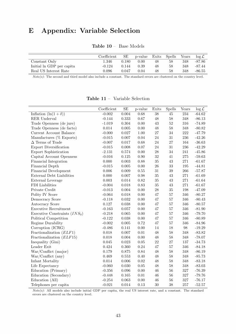
E Appendix: Variable Selection
Table 10 – Base Models
Coefficient SE p-value Exits Spells Years logLConstant Only 1.346 0.180 0.00 48 58 348 -87.86Initial ln GDP per capita -0.124 0.144 0.39 48 58 348 -87.44Real US Interest Rate 0.096 0.047 0.04 48 58 348 -86.55
Note(s): The second and third model also include a constant. The standard errors are clustered on the country level.
Table 11 – Variable Selection
Coefficient SE p-value Exits Spells Years logLInflation (ln(1 + δ)) -0.002 0.004 0.68 38 45 234 -64.62RER Underval -0.144 0.333 0.67 48 58 348 -86.13Trade Openness (de jure) -1.019 0.304 0.00 43 52 316 -74.89Trade Openness (de facto) 0.014 0.005 0.00 48 58 348 -80.82Current Account Balance -0.000 0.027 1.00 27 34 222 -47.79Manufactures (% Exports) -0.015 0.007 0.04 24 31 236 -42.26∆ Terms of Trade -0.007 0.017 0.68 24 27 164 -36.63Export Diversification -0.015 0.008 0.07 24 31 236 -42.29Export Sophistication -2.131 0.574 0.00 28 34 241 -45.86Capital Account Openness -0.016 0.125 0.90 32 41 275 -59.63Financial Integration 0.000 0.003 0.88 35 43 271 -61.67Financial Depth -0.015 0.005 0.00 26 33 195 -44.81Financial Development 0.006 0.009 0.55 31 39 266 -57.87External Debt Liabilities 0.000 0.007 0.98 35 43 271 -61.69External Leverage 0.003 0.014 0.82 35 43 271 -61.64FDI Liabilities -0.004 0.018 0.83 35 43 271 -61.67Private Credit -0.013 0.004 0.00 28 35 198 -47.09Polity IV Score -0.064 0.018 0.00 47 57 346 -80.27Democracy Score -0.118 0.032 0.00 47 57 346 -80.43Autocracy Score 0.127 0.038 0.00 47 57 346 -80.57Executive Recruitment -0.163 0.057 0.00 47 57 346 -81.90Executive Constraints (INS0) -0.218 0.065 0.00 47 57 346 -79.70Political Competition -0.122 0.038 0.00 47 57 346 -80.89Regime Durability -0.002 0.005 0.72 47 57 346 -84.96Corruption (ICRG) -0.486 0.141 0.00 14 18 98 -19.29Fractionalization (ELF1) 0.018 0.007 0.01 48 58 348 -83.82Fractionalization (ELF15) 0.018 0.004 0.00 48 58 348 -78.07Inequality (Gini) 0.045 0.023 0.05 22 27 137 -34.73Leader Exit 0.424 0.360 0.24 47 57 346 -84.18War/Conflict (major) 0.179 0.875 0.84 48 58 348 -86.19War/Conflict (any) 0.469 0.553 0.40 48 58 348 -85.73Infant Mortality 0.014 0.006 0.02 48 58 348 -83.18Life Expectancy -0.060 0.030 0.05 48 58 348 -83.03Education (Primary) -0.356 0.096 0.00 46 56 327 -76.39Education (Secondary) -0.448 0.165 0.01 46 56 327 -79.76Education (All) -0.254 0.063 0.00 46 56 327 -76.17Telephones per capita -0.021 0.014 0.13 30 38 257 -52.57
Note(s): All models also include initial GDP per capita, the real US interest rate, and a constant. The standarderrors are clustered on the country level.
43