this pdf is a selection from a published volume from the national ... · carlos henrique corseuil...

This PDF is a selection from a published volume from theNational Bureau of Economic Research

Volume Title: Law and Employment: Lessons from LatinAmerican and the Caribbean

Volume Author/Editor: James J. Heckman and Carmen Pagés,editors

Volume Publisher: University of Chicago Press

Volume ISBN: 0-226-32282-3

Volume URL: http://www.nber.org/books/heck04-1

Conference Date: November 16-17, 2000

Publication Date: August 2004

Title: The Impact of Regulations on Brazilian Labor MarketPerformance

Author: Ricardo Paes de Barros, Carlos Henrique Corseuil

URL: http://www.nber.org/chapters/c10072

5.1 Introduction

Labor market regulations are invariably introduced with two objectives.The first one is to improve the welfare of the labor force, even at the cost ofintroducing some degree of economic inefficiency. The second consists ofimproving efficiency, when external factors and/or other labor market im-perfections are present.

These regulations may eventually become inadequate due to an unsuit-able original design or unexpected changes in the economic environment.This inadequacy may lead to results contrary to the original goals of labormarket regulations. Consequently, as a general rule, labor market regula-tions (as any other market regulation) need to be constantly evaluated andupdated if their original goals are to be preserved.

However, any empirical study of the impact of labor market regulationson labor market performance faces three main difficulties. First, it is nec-essary to face the facts that labor market regulations do not change very of-ten and tend to apply universally to all sectors in the economy. Hence, vari-ations in labor market regulations, which are necessary to identify their

273

5The Impact of Regulationson Brazilian LaborMarket Performance

Ricardo Paes de Barros and Carlos Henrique Corseuil

Ricardo Paes de Barros is a researcher at the Institute for Applied Economic Research(IPEA), Brazil. Carlos Henrique Corseuil is a researcher at the Institute for Applied Eco-nomic Research (IPEA), Brazil.

This chapter is a compiled version of Barros, Corseuil and Gonzaga (1999) and Barros,Corseuil, and Bahia (1999). The authors would like to thank Wasmália Bivar for valuable in-formation about the PIM database. We also would like to thank Carmen Pagés, James Heck-man, Rosane Mendonça, Gustavo Gonzaga, Ricardo Henriques, and Miguel Foguel for com-ments on previous versions of this chapter. Finally, we cannot forget to mention the extremededication of our team in IPEA involved in this project, especially Mônica Bahia, PhillippeLeite, Danielle Milton, Eduardo Lopes, Gabriela Garcia, Viviane Cirillo, and Luis EduardoGuedes.

impact on labor market performance, are hard to find, both in time seriesand cross-sections.

Second, even when legislation varies over time, it is difficult to isolate itsimpact on labor market performance from the impact of other macroeco-nomic factors. This is particularly important in Brazil, because over thepast two decades macroeconomic instability has reached unprecedentedlevels. Inflation, economic growth, internal and external imbalances, andthe degree of openness of the economy have changed considerably. If oneopts for using cross-section variations, the drawbacks are not less. In thiscase, it is necessary to isolate the impact of differences in regulations fromall other sector-specific factors that could make performance measuresdifferent across sectors.

Finally, measures of labor market performance are needed. The problemhere is that performance is a multidimensional aspect of the labor marketwith no consensus about its precise definition. Hence, there is not a singleunidimensional measure for this aspect. The use of the measure for the(supposed) main dimension is usually implemented as a measure of labormarket performance.

In respect to the Brazilian labor market, many analysts have been verycritical about the benefits of the prevailing labor market regulations.1 Onthe whole, these regulations were designed to improve welfare, giving theworkers more protection. The analysts claim these regulations have notbeen wisely designed and, consequently, are failing to reach their objective.Actually their arguments go further, claiming that the regulation worsenednot only the welfare of the labor force, but also the efficiency, based on theobservation of increasingly poor working conditions and lower wages anda drop in the degree of employability of the Brazilian labor force. They ar-gue that this occurs in a new economic environment that increasingly re-quires greater labor flexibility. As a consequence, labor market regulationreform has become a central item on the current Congress agenda, partic-ularly after the recent leap in unemployment.2

Despite the importance of evaluations of the impact of these regulationson labor market performance, the number of such studies focusing onBrazilian labor markets has been very limited.3 The three difficulties pointedout are not sufficient to justify the relatively few studies on the subject. First,labor market regulations underwent considerable changes in 1988, when

274 Ricardo Paes de Barros and Carlos Henrique Corseuil

1. See Jatobá (1994) for a survey of those analyses that consider that a higher nonwage la-bor cost reduces the job creation. This survey includes the arguments of Bacha, Mata, andModenesi (1972), Camargo and Amadeo (1990), Almeida (1992), Chahad (1993), Macedo(1993), Pastore (1993), and World Bank (1991).

2. Deseasonalized unemployment in the six main Brazilian metropolitan regions increasedfrom around 5.7 percent in October 1997 to 7.4 percent in June 1998.

3. Some examples are Amadeo et al. (1995), Amadeo and Camargo (1993), Amadeo andCamargo (1996), and Málaga (1992).

a new constitution was enacted, containing most of the prevailing labormarket regulations. Moreover, the wealth of information available allowsthe implementation of promising methodological possibilities for identify-ing the impact of labor market regulations, based on alternative proxiesof labor market performance that can be obtained using the informationavailable.

Hence, the objective of this chapter is to identify whether the prevailingBrazilian labor market regulations, in large extension originated by the 1988constitutional change, have any impact on labor market performance. Toreach this objective we will explore alternative methodologies, sources ofinformation, and measures of labor market performance. The diversifica-tion is an attempt on accessing the robustness of our result.

We have two alternatives to measure labor market performance. The firstis based on parameters estimated from a labor demand model, and the sec-ond is based on turnover rates. Some alternative methodologies for estima-tion of the effect of the constitutional change are associated to each of thesetwo measures. Regression analysis is the only alternative developed for la-bor demand parameters estimation. The turnover rates are mainly analyzedthrough the difference-in-differences methodology, but regressions are alsodeveloped as a complement of the difference-in-differences method.

The chapter is organized in five sections, including this introduction. Inthe next section we briefly describe the 1988 constitutional change, withspecial emphasis on the topics related to labor costs, which, basically, willbe used as the main sources of variation on labor market regulations. Thetwo sections that follow the institutional analysis will focus on the two al-ternative measures of labor market performance. Section 5.3 is dedicatedto the description and implementation of the regression analysis throughwhich we estimate the parameters of labor demand. Section 5.4 containsthe description and results achieved when we use turnover rates to measurelabor market performance according to difference-in-differences method-ology complemented by regression analysis. Finally, section 5.5 summa-rizes our main findings.

5.2 The Institutional Analysis

5.2.1 The 1988 Constitutional Change

A new Brazilian Constitution was enacted in 1988 as part of the processof redemocratization in Brazil during the second half of the 1980s. Tradi-tionally, Brazilian constitutions are very detailed, stipulating not only gen-eral rules, but also many specific legal provisions. Most labor regulations,for instance, are written in the constitution and are, consequently, verydifficult to amend. The new constitution of 1988, in particular, consider-

Impact of Regulations on Brazilian Labor Market Performance 275

ably affected labor regulations, causing changes in many labor codes thathad remained intact since the 1940s.4 Most of these changes, in tune withthe redemocratization environment, increased the degree of the workers’protection.

These changes, shown in table 5.1, affected both individual rights andworkers’ organizations. The new constitution gave more freedom and au-tonomy to unions. The possibilities for government intervention in unionswere drastically reduced. In fact, many mechanisms of official interferencewere eliminated (e.g., the right of intervention by the Ministry of Laborand the need to be registered and approved at the same Ministry) as well asmany restrictions of an institutional nature used to limit workers’ organi-zations (such as representation scales and diversity of occupational cate-gories). Many regulations on union management were also weakened, en-suring more autonomy to unions during elections of their representativesand in their decisions.

From the point of view of individual rights, we can perceive importantchanges that increase variable labor costs and the level of dismissal penal-ties. The increase in protection ensured by the new constitution consider-ably increased a firm’s costs of employment. The maximum number ofworking hours per week dropped from forty-eight to forty-four hours; themaximum number of hours for a continuous work shift dropped from eight to six hours; the minimum overtime premium increased from 20 per-cent to 50 percent; maternity leave increased from three to four months;and the value of paid vacations increased from 1 to, at least, 4/3 of the nor-mal monthly wage.

The new constitution also considerably increased the level of dismissalpenalties. This change in legislation will be one of the fundamental sourcesof variation used throughout this study to estimate the impact of regula-tions on labor market performance.

It is worth mentioning that the changes altered the level of the penaltiesbut not their nature. Traditionally, Brazilian legislation affects the cost ofdismissal through two channels. First, employers must give notice to theiremployees in the case of dismissal. Moreover, between the notice and ac-tual dismissal, workers are granted two hours per day to look for a new job,with no cut in wages. Second, the law states that all workers dismissed forno just cause must receive monetary compensation paid by the employer.

Prior to the 1988 constitution, notice had to be given at least one monthin advance. The 1988 constitution states that the period of notice should begiven in proportion to the worker’s tenure. However, because no specific lawhas ever regulated this constitutional device, notice continues to be given,as before 1988, one month prior to dismissal for all workers, independent


4. One major exception was the rule regulating dismissals, which suffered major changes in1966 when the FGTS was created.

Tab

le 5

.1C

hang

es I

ntro

duce

d by

the

New

Con

stit

utio

n P

rom

ulga

ted

in O

ctob

er 1

988

Pre

-Con

stit

utio

nPo

st-C

onst

itut

ion

Indi

vidu

al R

ight

s1.

Max

imum

wor

king

hou

rs p

er w

eek

�48

hou

rs.

1. M

axim

um w

orki

ng h

ours

per

wee

k �

44 h

ours

.2.

Max

imum

dai

ly jo

urne

y fo

r co

ntin

uous

wor

k sh

ift �

8 ho

urs.

2. M

axim

um d

aily

jour

ney

for

cont

inuo

us w

ork

shif

t �6

hour

s.3.

Min

imum

ove

r-ti

me

rem

uner

atio

n �

1,2

of th

e no

rmal

wag

e ra

te.

3. M

inim

um o

ver-

tim

e re

mun

erat

ion

�1,

5 of

the

norm

al w

age

rate

.4.

Pai

d va

cati

ons

�at

leas

t the

nor

mal

mon

thly

wag

e.4.

Pai

d va

cati

ons

�at

leas

t 4/3

of t

he n

orm

al m

onth

ly w

age.

5. M

ater

nity

lice

nse

�3

mon

ths

(1 b

efor

e an

d 2

afte

r th

e bi

rth)

.5.

Mat

erni

ty li

cens

e �

120

days

.6.

Pre

viou

s no

tific

atio

n of

dis

mis

sal �

one

mon

th.

6. P

revi

ous

noti

ficat

ion

of d

ism

issa

l �pr

opor

tion

al to

sen

iori

ty (t

o be

reg

u-la

ted

by a

futu

re la

w).

7. F

ine

for

nonj

usti

fied

dism

issa

l �10

% o

f Fun

do d

e G

aran

tia

por

Tem

po d

e 7.

Fin

e fo

r no

n-ju

stifi

ed d

ism

issa

l �40

% o

f Fun

do d

e G

aran

tia

por

Tem

po

Serv

iço

(FG

TS)

.de

Ser

viço

(FG

TS)

.8.

Cre

atio

n of

pat

erni

ty li

cens

e of

5 d

ays.

9. P

rofit

-sha

ring

(reg

ulat

ed b

y a

1996

/97

law

).

Uni

ons

Org

aniz

atio

nA

) T

he M

inis

try

of L

abor

had

the

righ

t to

inte

rven

e in

the

unio

ns a

nd d

epos

e A

) T

he M

inis

try

of L

abor

is fo

rbid

den

to in

terv

ene

in th

e un

ions

.th

eir

boar

d of

dir

ecto

rs.

B)

Eve

ry u

nion

had

to b

e re

gist

ered

and

app

rove

d at

the

Min

istr

y of

Lab

or.

B)

Uni

ons d

o no

t nee

d to

be

regi

ster

ed a

nd a

ppro

ved

at th

e M

inis

try

of L

abor

.C

) N

atio

nal r

epre

sent

atio

n of

uni

ons

was

allo

wed

onl

y in

exc

epti

onal

cas

es.

C)

Nat

iona

l rep

rese

ntat

ion

of u

nion

s is

allo

wed

.D

) Uni

on’s

rep

rese

ntat

ives

wer

e el

ecte

d by

a m

inim

um q

uoru

m o

f 2/3

of t

he

D)U

nion

’s r

epre

sent

ativ

es a

re e

lect

ed fo

llow

ing

unio

n’s

own

rule

s.m

embe

rs in

the

first

bal

loti

ng, 1

/2 in

the

seco

nd b

allo

ting

and

2/5

in th

e th

ird

ballo

ting

. In

the

case

of n

o m

inim

um q

uoru

m fo

r th

e el

ecti

on, t

he

Min

istr

y of

Lab

or c

ould

cho

ose

unio

n’s

dire

ctor

s an

d ca

ll an

othe

r el

ecti

on.

E)

Wor

kers

(em

ploy

ers)

uni

ons

wer

e al

low

ed to

be

form

ed b

y on

ly o

ne ty

pe

E)

Wor

kers

(em

ploy

ers)

uni

ons

are

allo

wed

to b

e fo

rmed

by

diff

eren

t typ

es o

f oc

cupa

tion

al (e

cono

mic

) cat

egor

y.oc

cupa

tion

al (e

cono

mic

) cat

egor

ies.

F)

Uni

on’s

dec

isio

n to

go

on s

trik

e ha

d to

be

appr

oved

by

a m

inim

um q

uoru

m

F)

Uni

on’s

dec

isio

n to

go

on s

trik

e fo

llow

s un

ion’

s ow

n cr

iter

ias.

of 2

/3 o

f uni

on’s

mem

bers

in th

e fir

st c

allin

g an

d 1/

3 in

the

seco

nd c

allin

g.G

) In

case

of s

trik

e, n

otifi

cati

on to

the

empl

oyer

had

to b

e do

ne 5

day

s in

G

)In

case

of s

trik

e, n

otifi

cati

on to

the

empl

oyer

has

to b

e do

ne 4

8 ho

urs

in

adva

nce.

adva

nce.

H) S

trik

es w

ere

forb

idde

n in

act

ivit

ies

cons

ider

ed fu

ndam

enta

l (e.

g., e

nerg

y H

) The

re a

re n

ot a

ny m

ore

sect

ors

in w

hich

str

ikes

are

forb

idde

n: I

n es

sent

ial

and

gas

serv

ices

, hos

pita

ls, p

harm

acie

s, fu

nera

l ser

vice

s); p

ublic

ser

vant

s ac

tivi

ties

, wor

kers

and

em

ploy

ers

are

resp

onsi

ble

for

the

prov

isio

n of

min

-w

ere

not a

llow

ed to

go

on s

trik

e.im

um s

ervi

ces;

pub

lic s

erva

nts

(exc

ludi

ng m

ilita

ry p

erso

nnel

) are

allo

wed

to

go

on s

trik

e.

Sou

rces

:Cam

argo

and

Am

adeo

(199

0) a

nd N

asci

men

to (1

993)

.

of their tenure. Hence, it cannot be used as our source of variation in laborregulations.

Concerning the monetary compensation for dismissed workers, the lawstates that a fixed percentage of the Fundo de Garantia por Tempo de Serviço(FGTS), a sort of job security fund accumulated while the worker was em-ployed by the firm, is to be paid to every worker dismissed for no just cause.There was a fourfold increase in the value of this penalty as a result of the1988 constitutional change.

The basic characteristics of the FGTS are the following. First, eachworker in the formal sector has his own fund; in other words, it is a privatefund instead of a single fund for the workers as a group. Second, to buildthe fund of each individual worker, the employer must contribute, everymonth, the equivalent of 8 percent of his employee’s current monthly wage;consequently, the accumulated FGTS of a worker in any given firm is pro-portional to the worker’s tenure and his or her average wage over his or herstay in the firm. Third, the fund is administrated by the government. Fourth,workers have access to their own fund only if dismissed without just causeor upon retirement.5 Fifth, if they resign they are not granted access to thisfund. Sixth, on dismissal, workers have access to their entire fund, includ-ing all funds accumulated in previous jobs, plus a penalty in proportion totheir accumulated fund in the job from which they are being dismissed.6

Before 1988, this compensation was equal to 10 percent of the cumula-tive contribution of the current employer to the worker’s FGTS. After1988, this penalty was increased to 40 percent of the employer’s cumulativecontribution to the worker’s FGTS. As the monthly rate is 8 percent of themonthly wage, the FGTS accumulates at a rate of approximately one fullmonthly salary per year in the job. So, quantitatively, the penalty accu-mulates in a rate equivalent to 40 percent (10 percent prior to 1988) of theworker’s current monthly wage per year in the firm. This compensation wascertainly very small prior to 1988. In fact, under the former constitution,the worker had to be employed in the firm for at least ten years in order forthe compensation to reach the magnitude of one monthly salary. Now ittakes 2.5 years in the job for the compensation to reach this value.

Finally, it is worth mentioning that despite the 1988 fourfold increase inthe FGTS penalty it is not clear that, even now, this penalty constitutes amajor constraint to dismissals or even a major fraction of overall dismissalcosts. For instance, the cost of advance notice may be larger than thepenalty. In principle, the need for notice would increase the cost of dis-missal only to the extent that, for a period of one month, 25 percent of the


5. There are a few exceptions. Workers can use their FGTS as a part of the payment for ac-quiring their home. They also can use it to pay for large health expenses.

6. The FGTS is a fund created by the military regime in 1966 to serve as an alternative tothe job security law prevailing at that time. In practice, all new contracts after 1966 adoptedthe new system because it was preferred by both employees and employers.

hours of the dismissed worker would be paid but not worked. In practice,the productivity of a dismissed worker will drop once he or she has beengiven notice, implying an overall decline of well over 25 percent in his orher contribution to production. As a result, it is not uncommon for firmsto pay a full salary to dismissed workers, without their being required towork a single hour. In other words, the cost of notice is actually between 25percent and 100 percent of one month’s salary, being in practice closer to100 percent than to 25 percent.

Consequently, the costs of advance notice tend to be higher than the dis-missal compensation paid to all workers with tenure of less than 2.5 years.Because most employment relationships in Brazil are short, employers maybe more sensitive to the cost of advance notice than to the value of the dis-missal compensation.

5.2.2 Dismissal Penalties, Incentives, and Possible Labor Market Outcomes

As far as incentives are concerned, it is worth emphasizing that beingfired is the chief mechanism to achieve access and control over their over-all FGTS. Furthermore, there are strong incentives for workers to seek ac-cess to their FGTS. First, the FGTS has been poorly managed by the gov-ernment, typically generating negative real returns or returns well belowmarket rates.7 Second, due to shortsightedness or credit constraints, work-ers may be heavily discounting the future. The facts that (1) all dismissalpenalties are immediately received individually by the dismissed worker,and (2) being dismissed is the chief mechanism for workers to acquire con-trol over their own fund that is poorly managed by the government givethem considerable incentives to induce their own dismissal after a certaintime in any job. However, those incentives are related to the existence of theFGTS and the amount accumulated in this fund. As we saw in the last sec-tion, the constitution did not change those aspects of regulation.

There are other incentives associated with the dismissal penalty that mayindeed drive the results estimated on this paper. On one hand this penaltyis paid by the employer to the employee, as opposed to the employer’s pay-ing into a social fund held for all workers as a group. In other words, thedismissed worker (only him) receives the penalty on an individual basis.This characteristic of the law has well-established and major negative ef-fects on the workers’ behavior, giving them significant incentives to inducetheir own dismissal.8

On the other hand, firm behavior tends, however, to reduce dismissalswhen there is an increase on the dismissal’s penalties value. Additionally,


7. See Almeida and Chautard (1976) for a broad analysis of the FGTS, including topicssuch as management of the fund and workers’ welfare. Carvalho and Pinheiro (1999) providea more updated analysis, focusing on the role of FGTS on fomenting investments.

8. See Macedo (1985) and Amadeo and Camargo (1996).

as a result of the increase in dismissal penalties, firms become more selec-tive in their hiring procedures, leading to an overall decline even greater indismissal rates. Hence, the net effect on turnover will depend on the re-spective responses’ intensities of each part (firms and workers) to the mag-nitude of the penalties. It is worth mentioning that these incentives are as-sociated with employment spells longer than three months because beforethat employers can fire workers free of any penalty.

Hence, the aggregate effect on turnover will depend also on the firm re-action during the first months of the relation, namely the training period.The firm may become more selective in the first three months because thefiring process becomes more expensive later. It means that the turnovermay increase during this period as a consequence of an increase on dis-missal penalties. So we have to contrast the results related to both periodsin order to access the aggregate result on turnover.

According to the incentives described previously, it is not clear that leg-islation would achieve the original goal of a lower firing level. We can ei-ther have an opposite or null result. Additionally, a null net result can alsoarise from the absence of any reaction. This would be the case if the penaltyis not a bidding constraint. In fact, we have some evidence that workers andfirms collude to turn voluntary quits into dismissals. Under this circum-stance workers can have access to their fund, but firms do not pay anypenalty. Barros, Corseuil, and Foguel (2001) show that approximately 2/3of the workers that voluntarily quit from jobs in the formal sector accesstheir FGTS, which means that these quits were officially registered as dis-missals.9

5.3 Demand for Labor Estimation

This part of the chapter describes an attempt to estimate the impact ofregulations on labor market performance based on the first of the two mea-sures mentioned in the introduction—the labor demand parameters. Theseparameters constitute our proxy for labor market performance. As we esti-mate the parameters monthly, we can try to identify whether the evolutionof these parameters is associated to the constitutional change or to the evo-lution of macroeconomic indicators. This exercise constitutes our secondstep, where we run regressions of the labor demand parameters on an indi-cator of the constitutional change and on macroeconomic indicators.

This part is organized in five sections. Section 5.3.1 describes a structuralmodel for labor demand on which we base our first step. The estimationprocedure of the relation suggested by the theoretical model is described insection 5.3.2. The second step and a data base description are the focus ofsections 5.3.3 and 5.3.4, while the results of both steps are commented onin section 5.3.5.


9. There are questions about access to the fund in some Brazilian household surveys.

5.3.1 A Structural Model for Labor Demand

In this section we estimate a structural dynamic labor demand model us-ing longitudinal data on establishments. The model, one of the most simplein the literature, assumes labor as a homogeneous input and that labor isthe only input undergoing adjustment costs.10 Moreover, this basic theo-retical model assumes that each firm i, at each point in time t, chooses thelevel of employment, ni (t), in order to maximize the expected present valueof profits; that is, each firm chooses ni (t) in order to maximize

(1) Et�∑�

r�0

�r{R[ni (t � r), pi (t � r), �(t � r), � i (t � r)]

� �(t � r)wi (t � r)ni (t � r) � C [�ni (t � r), (t � r)]}�,

where R is the revenue function and C is the employment adjustment costfunction.

Hence, at each point in time the revenue function, R, can be obtained bychoosing the level of production and of all nonlabor variable inputs thatmaximize a current profits condition on a given choice for employmentand the state of the technology.11 As a consequence, the arguments of therevenue function can be divided into three groups: (1) level of employment,ni (t); (2) price of all other variable inputs relating to the product price, pi (t);and (3) all factors determining the state of technology. We divide the fac-tors determining the state of technology into two groups: (1) a vector of pa-rameters defining the overall form of technology at each point in time, �(t),that is common to all firms; and (2) a certain firm and time-specific tech-nological innovation, �i (t).

The second term in equation (1) is the direct cost of labor. In this equa-tion, wi (t) is the real wage rate12 paid by firm i at time t, and �(t) is the ratiobetween the overall variable cost of labor and the wage rate. We are im-plicitly assuming that all nonwage variable costs are proportional to wageswith the proportionality constant and common to all firms but possiblytime varying due to changes in the legislation.

Finally, the cost of adjustment (C ) is assumed to be a function of the netchange in employment, �ni (t) � ni (t) – ni (t – 1), and a parameter, (t). Thisparameter may vary over time to capture changes in the economic envi-ronment and in the labor legislation, but it is common to all firms, indicat-ing that all firms face the same adjustment cost.

According to this model, the form of technology and labor costs mayvary freely over time. However, idiosyncratic shocks of a firm can only


10. See Nickell (1986), Hamermesh (1993), and Hamermesh and Pfann (1996) for surveysof dynamic labor demand models.

11. In the state of the technology, we include the impact of the level of all fixed or exoge-nously determined inputs.

12. The real wage rate is obtained by dividing the nominal wage rate by the product price.

affect technology. Labor costs are determined by firm-specific wages and alegislation that is common to all firms.

In order to obtain an explicit solution to this problem of maximization,we introduce a series of simplifying assumptions that allow us to write thesolution of equation (1) as the following expression defined for the em-ployment level:13

(2) ni (t) � ni (t � 1) � �(1

�

�12

)� ��11(t) � � i(t) � ∑

m

s�1

ϕs(t)Iis � �(t)wi(t)�,

where is implicitly defined by

�12 � (1 � )(1 � �),

and Iis indicates whether firm i belongs to sector s, that is, Iis � 1 if firm i be-longs to sector s and Iis � 0 otherwise. Finally, �11(t), �12(t) are originatedfrom �(t) and correspond to parameters of a quadratic revenue function,the same assumption made for the adjustment cost function.

5.3.2 Econometric Specification

To obtain an empirically feasible econometric specification for the de-mand for labor, we must be more specific about the firm- and time-specifictechnological innovation, � i(t). We assume that this innovation consists ofthree underlying components; that is, we assume that

� i(t) � i � �(t) � Ui (t),

where i captures a firm-specific, time-invariant technological component,� (t) an aggregated time-specific technological shock, and Ui(t) captures allother technological shocks. The presence of the first two components al-lows us to assume, without any loss of generality, that the average of Ui(t)over time and across firms is always zero. However, because the economet-ric model will also include sectorial indicators, Iis , we must assume that theaverage of Ui(t) within each sector is also zero; that is, we assume that forevery s,

E[Ui(t)Iis � 1] � 0.

To identify the parameters of the model, additional assumptions are re-quired. Probably the simplest route to obtain identification is to assume thatUi(t) is an exogenous moving-average process. Accordingly, we assume that

E[Ui(t)ni (t � p)] � 0

for all p � k1. We also assume that although these technological shocksmay be correlated with the recent evolution wages, they are uncorrelatedwith the evolution of wages in the past; that is,


13. The complete derivation of the model is reported in appendix A.

E [Ui(t)wi (t � p)] � 0

for all p � k2. Notice that if U were an exogenous moving-average processof order

k � max(k1, k2),

then these two assumptions would be immediately satisfied.Given this specification for the technological innovation, equation (2)

may be rewritten as

(3) ni(t) � �(t) � ∗i � ∑

m

s�1

ϕs∗(t)Iis � �∗(t)wi (t) � ni (t � 1) � Ui

∗(t),

where

�(t) � �1

�

�12

� [�11(t) � �(t)],

i∗(t) � �

1

�

�12

� i ,

�∗(t) � �1

�

�12

��(t),

ϕs∗(t) � �

1

�

�12

� (t),

Ui∗(t) � �

1

�

�12

�Ui(t).

The presence of �(t) and i∗ in equation (3) poses some drawbacks for es-

timation. The presence of �(t) makes estimation of the other parametersunfeasible in a pure time series context, unless some function form for �(t)is imposed.

In a cross-section environment, the difficulty is imposed by the naturalcorrelation between i

∗ and ni (t – 1). To solve this problem we must rely onlongitudinal information. When this type of information is available, wecan take first differences to obtain

(4) �ni (t) � ��(t) � ∑m

s�1

�ϕs∗(t)Iis � �∗(t)�wi (t) � �ni (t � 1) � �U i

∗(t),

as long as the ratio between the overall variable cost of labor and the wagerate � (t) is time invariant. This equation has the advantage of eliminatingthe idiosyncratic component i

∗. Nevertheless, it still cannot be estimatedas a multiple regression because

E [�ni (t � 1)�Ui∗(t)] � 0.

However, it follows from the assumptions made previously about Ui(t)that


E [ni (t � p)�Ui∗(t)] � 0,

and

E [wi (t � p)�Ui∗(t)] � 0

for all p � k � 1. Hence, the model can be estimated by instrumental vari-able using past values of employment and wages as instruments. Under theassumptions made on Ui(t), all values of employment and wages lagged atleast k � 2 periods would be valid instruments. However, from a practicalpoint of view it is necessary to limit the number of instruments. In thisstudy we use as instruments 6 lags for employment and 6 lags for wages;that is, we use as instruments employment and wages lagged, k � 2, . . . ,k � 7 months. In the estimation we use two alternative values for k (onemonth and ten months). Hence, to implement this econometric procedureit is necessary to count with panel information at least seventeen monthslong on firm-specific employment and wages.

Using this econometric model, based on equation (4), it is possible to es-timate � (t), , �∗, and ϕs (t). Changes on the values of these parameters, es-pecially and �∗ after 1988, indicate that the regulation might have im-pacted on labor market performance.14 One possibility for investigatingthese possible changes would be to estimate two sets of parameters, first us-ing data from the years before 1988 and then data from recent years. Theavailable data allows us to obtain monthly estimates of the parameters ofthe demand function.

This strategy has at least three advantages over the strategy of estimat-ing just two models for a period before and after 1988. First, it is easier toimplement because the econometric model is essentially estimated in across-section. This feature of the estimation procedure makes estimatingthe standard errors much easier because in this case it is not necessary toestimate the temporal correlation patterns of the technological shocks.

Second, the estimation of a model for every month has the great advan-tage of allowing a precise identification of the exact point in time where theparameters have changed. A precise identification of the moment when theparameters changed can provide important insights into the question ofwhether the constitutional change is the real force behind the changes inthe demand for labor. For instance, if the parameters began to change longbefore or long after 1988, we would become suspicious about the causal


14. At this point it is worthwhile mentioning that, although the demand for labor is esti-mated for every month, in the estimation procedure the parameters �12, , and � must be atleast locally time invariant. The estimated parameters are consistent only if this assumptionis valid. If the parameters �12 and change over time, equation (2) would not be the solutionof the Euler equation. Moreover, if � varies from one month to the next, the first differencemade to eliminate the firm-specific time invariant technological component, i

∗, would stillwork but would generate a different function form to be estimated because in this case �∗would not factor out.

link between the 1988 constitutional change and those in the demand forlabor.

Third, and more important, monthly estimations of the parameters al-low us to identify in which sense their evolutions are determined—by theregulation (1988 constitutional change) or by the evolution of macroeco-nomic indicators. This is precisely what we do in the second step of this re-gression analysis.

In the next section we describe this second step in detail. It is worth men-tioning that we can also obtain estimated values for coefficients of interestother than the ones mentioned previously. The first of these other coeffi-cients is the long-run impact of changes in wages on employment, �, thatcan be obtained via

� � �(1

�

�

∗

)�.

Other parameters of interest are the structural parameters of the pro-duction function, �12, and of the cost function, . Some additional infor-mation is required to obtain estimated values for these parameters. In thisstudy, to recover these original parameters we assume that the discountrate, �, and the ratio between the unit cost of labor and the wage, �, areknown and equal to 0.95 and 1.8, respectively. Given the knowledge ofthese two parameters and estimates for and �∗, estimates for the under-lying parameters �12 and can be obtained via

�12 � �1

�

�

∗

�

and

� ��∗(1

�

�

�)� .

5.3.3 Identification Strategy: The Second Step

The monthly estimate of demand functions was just the first step in oureconometric strategy. Because the Brazilian economy underwent a processof trade liberalization and was subject to a series of stabilization plans atthe same time as the change in the constitution, changes in the parametersof the labor demand function that may have occurred over this period can-not be immediately attributed to the constitutional change.

To isolate the effect of the constitutional change on the parameters of thedemand function, we regress our monthly estimates of these parameters ona temporal indicator for the 1988 constitutional change, Dt , controlling fora variety of other macroeconomic indicators, Mt . Because the precision ofestimates varies considerably over time, to control for this source of varia-tion we use as our dependent variable the parameter estimate divided by its


corresponding standard error. More specifically, we estimate the followingregressions

�s

(

(

t

t

)

)� � a1 � b1D(t) � c1M(t) � e1(t)

and

��

s

∗

�(

(

t

t

)

)� � a2 � b2D(t) � c2M(t) � e2(t),

where s(t) and s�(t) are the standard errors of (t) and �∗(t), and D(t) � 0,if t refers to a period prior to 1988 and D(t) � 1 otherwise. We include thefollowing as macroeconomic indicators: (1) the GDP real growth rate;(2) degree of openness measured by the ratio of total trade (exports plusimports) to the GDP; (3) inflation rate; and (4) inflation volatility mea-sured by the inflation standard deviation. Monthly dummies and a lineartrend were included in all regressions. These regressions are estimated byordinary least square method using monthly data covering the period June1986 to December 1997. Positive and statistically significant estimates forb1 and b2 would then be taken as evidence that the 1988 constitutionalchange had an important effect on the demand for labor and, consequently,on the level of employment and the speed of adjustment.

5.3.4 The Database

In the first step of the regression analysis we estimate the demand for la-bor using monthly longitudinal information from the Pesquisa IndustrialMensal (PIM). The PIM is a monthly industrial establishment survey con-ducted by the IBGE (Brazilian Census Bureau), covering the entire coun-try. It is a longitudinal survey of a stratified sample of approximately 5,000manufacturing establishments employing five workers or more. The panelcovers the period from January 1985 to the present.

The survey collects information on labor inputs, labor costs, turnover,the value of production, and so on. The data on labor inputs includes bothemployment and the total number of hours paid. The survey has three ma-jor limitations in terms of measuring labor inputs. First, the informationcovers the total number of hours paid but not the actual number of hoursworked. Second, all data refers only to the personnel directly involved inproduction. Finally, there is no information on the qualification of the la-bor force employed.

In relation to labor costs, two types of information are available: (1) to-tal value of contractual wages (that is, value of wages and salaries as spec-ified in labor contracts), and (2) total value of payroll. For the purposes ofthis study, the payroll data seems to be more informative because it includes,in addition to contractual wages, the payment for overtime, commissions,and other incentive schemes, such as a productivity premium. It also in-


cludes all fringe benefits; paid vacations; and any additional payments forhazardous activities, night shifts, and other compensating schemes.15

Despite the fact that the payroll data covers a wide variety of labor costs,it does not include all of them. Major exceptions are the employer’s con-tributions to social security, training programs, and other social programs.Fortunately, however, these contributions as fractions of contractual wageshave been fairly constant over time, except for a significant change for theoccasion of the 1988 constitution.

Hence, for each establishment in the survey we use essentially threepieces of information: (1) employment level, (2) total number of hourspaid, and (3) total payroll. Basing our information on these three variableswe construct two measures for variable labor cost. These two measures areobtained by dividing total payroll by the level of employment and the totalnumber of hours paid, respectively. For labor input we use both availablemeasures: employment and hours paid. As a result, each demand model isactually estimated twice, depending on whether labor inputs are measuredby employment or hours paid. We will refer to the one based on employ-ment level as model 1 and to the one based on hours paid as model 2.

In the first step of the regression analysis we aggregate some macroeco-nomic indicators mentioned in the last section. The source of the gross do-mestic product (GDP) data is the IBGE. The data for exports and importswas calculated in joint work by the Fundação Centro de Estudos deComércio Exterior (FUNCEX) and IPEA. Finally, we used the official in-flation index to measure inflation.

Before we move to the labor demand estimates, we present some basicstatistics from our sample of establishments. Panels A and B of figure 5.1present the monthly evolution of the average level of the two measures oflabor input used in the study. These figures reveal that firms in our sampleemploy 200 to 300 workers who are paid a total of 45,000 to 70,000 hoursper month during the period analyzed. The average number of hours paidper month per worker in our sample is around 230 hours. Notice that afraction of the hours paid is not actually worked. For instance, included inthe hours paid is at least one day off per week (usually Sunday), which ispaid but not worked.

All these figures reveal that, over the 1985–1997 period, employmentand hours paid per manufacturing firm declined considerably, with the to-tal decline concentrated in the first two years of the 1990s. The main goalof this study is to determine precisely to what extent this decline can be as-sociated with the 1988 constitutional change or with other macroeconomic


15. In this study, all information on contractual wages and payroll has been deflated usingthe sector’s specific wholesale price index, except for the pharmaceutical; plastic; textile; andperfume, soap, and candle sectors. All monetary values referred to constant reais at Decem-ber 1997.

A Fig

. 5.1

Bas

ic S

tati

stic

s: A

,Ave

rage

em

ploy

men

t per

est

ablis

hmen

t; B

,ave

rage

num

ber

of h

ours

pai

d pe

r m

onth

per

est

ablis

hmen

t;

C,p

ayro

ll pe

r pr

oduc

tion

wor

ker;

D,p

ayro

ll pe

r ho

urs

paid

; E,e

volu

tion

of m

onth

ly in

flati

onS

ourc

es: A

, B, C

,and

D,b

ased

on

the

PIM

; E,t

he I

BG

E.

Not

e: E

,infl

atio

n m

easu

red

by th

e va

riat

ion

in Í

ndic

e N

atio

nal d

e P

reço

ao

Con

sum

idor

(IN

PC

-R) f

rom

the

15th

of o

ne m

onth

to th

e 15

th o

f the

sub

se-

quen

t mon

th.

B Fig

. 5.1

(con

t.)

C Fig

. 5.1

(con

t.) B

asic

Sta

tist

ics:

A,A

vera

ge e

mpl

oym

ent p

er e

stab

lishm

ent;

B,a

vera

ge n

umbe

r of

hou

rs p

aid

per

mon

th p

er e

stab

lishm

ent;

C

,pay

roll

per

prod

ucti

on w

orke

r; D

,pay

roll

per

hour

s pa

id; E

,evo

luti

on o

f mon

thly

infla

tion

Sou

rces

: A, B

, C,a

nd D

,bas

ed o

n th

e P

IM; E

,the

IB

GE

.N

ote:

E,i

nflat

ion

mea

sure

d by

the

vari

atio

n in

Índi

ce N

atio

nal d

e P

reço

ao

Con

sum

idor

(IN

PC

-R) f

rom

the

15th

of o

ne m

onth

to th

e 15

th o

f the

subs

eque

ntm

onth

.

D Fig

. 5.1

(con

t.)

E Fig

. 5.1

(con

t.) B

asic

Sta

tist

ics:

A,A

vera

ge e

mpl

oym

ent p

er e

stab

lishm

ent;

B,a

vera

ge n

umbe

r of

hou

rs p

aid

per

mon

th p

er e

stab

lishm

ent;

C

,pay

roll

per

prod

ucti

on w

orke

r; D

,pay

roll

per

hour

s pa

id; E

,evo

luti

on o

f mon

thly

infla

tion

Sou

rces

: A, B

, C,a

nd D

,bas

ed o

n th

e P

IM; E

,the

IB

GE

.N

ote:

E,i

nflat

ion

mea

sure

d by

the

var

iati

on in

Índ

ice

Nat

iona

l de

Pre

ço a

o C

onsu

mid

or (

INP

C-R

) fr

om t

he 1

5th

of o

ne m

onth

to

the

15th

of

the

subs

eque

ntm

onth

.

changes that marked the performance of the Brazilian economy over thisperiod.

Panels C and D of figure 5.1 show the monthly evolution of our two mea-sures for labor costs. These figures reveal that average wages (in Brazilianreais [R]) for production workers in Brazilian manufacturing were, most ofthe time, between R$600 and R$800 per month, leading to an hourly wagerate between R$2.50 and R$3.50.16 These figures reveal an overall upwardtrend in wages over the period, coupled with at least four cyclical fluctua-tions. These cycles very closely match series of stabilization plans thatmarked the period 1985–1994; see panel E of figure 5.1.

5.3.5 Empirical Results

The 1988 constitutional change brought an increase in labor costs, firingcosts in particular. To the extent that this change was of substantial im-portance, it would lead to a decline in the response of employment towages, �∗ and �, and also in the speed of adjustment (i.e., an increase in thecoefficient on lag employment, ).

We estimate labor demand models for each month from June 1986 toDecember 1997. Although we have information since January 1985, theneed for valid instruments determines that parameter estimates could onlybe obtained from mid-1986, that is, seventeen months after the actualsample information begins.

As already mentioned in the previous sections, two labor demand mod-els were estimated, depending on the choices of measures for labor inputs.Moreover, two estimates are obtained for each model, depending on howfar in the past we select the instruments. In total, four estimates for the la-bor demand function are obtained. In each case we directly estimate twobasic parameters: (1) the coefficient on lag employment, ; and (2) the co-efficient on current wages, �∗. We also obtain estimates for the long-runimpact of change in wages on employment (�) and other structural pa-rameters (�12 and ).

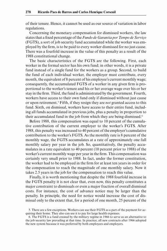
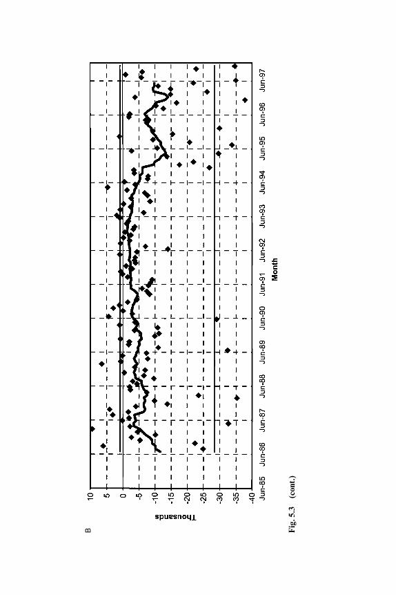
Figures 5.2 and 5.3 provide estimates of the monthly evolution of theshort-run impact of changes in wages on employment, �t

∗. Figures 5.4 and5.5 show corresponding estimates for the coefficient on lag employment,t . Because the estimates vary considerably from month to month, we alsocompute a trimmed twelve-month moving average. We adopted a two-stepprocedure to calculate this moving average. First, we eliminate all values inthe lowest and highest tenths of the distribution.17 Second, we calculate thetwelve-month moving averages with the remaining estimates. The averagesare weighted, using the inverse of the standard errors of each estimate asweights. Basing our information on these moving average estimates for the


16. The exchange rate was 1.11 R$/US$ in December of 1997.17. In each figure, the lowest and highest tenths are indicated by two horizontal lines.

A Fig

. 5.2

Tem

pora

l evo

luti

on o

f the

sho

rt-r

un re

spon

se o

f em

ploy

men

t to

labo

r co

sts

vari

able

(–�

∗ ), v

aria

ble

in le

vel.

Mod

el 1

: Em

ploy

-m

ent l

evel

: A,k

�1;

B,k

�10

Sou

rce:

Bas

ed o

n th

e P

IM.

B Fig

. 5.2

(con

t.)

A Fig

. 5.3

Tem

pora

l evo

luti

on o

f the

sho

rt-r

un re

spon

se o

f em

ploy

men

t to

labo

r co

sts

vari

able

(–�

∗ ), v

aria

ble

in le

vel.

Mod

el 2

: Hou

rs p

aid:

A,k

�1;

B,k

�10

Sou

rce:

Bas

ed o

n th

e P

IM.

B Fig

. 5.3

(con

t.)

A Fig

. 5.4

Tem

pora

l evo

luti

on o

f the

sho

rt-r

un re

spon

se o

f em

ploy

men

t to

lagg

ed e

mpl

oym

ent v

aria

ble

(�),

var

iabl

e in

leve

l. M

odel

1:

Em

ploy

men

t lev

el: A

,k�

1; B

,k�

10S

ourc

e:B

ased

on

the

PIM

.

B Fig

. 5.4

(con

t.)

A Fig

. 5.5

Tem

pora

l evo

luti

on o

f the

sho

rt-r

un re

spon

se o

f em

ploy

men

t to

lagg

ed e

mpl

oym

ent v

aria

ble

(�),

var

iabl

e in

leve

l. M

odel

2:

Hou

rs p

aid:

A,k

�1;

B,k

�10

Sou

rce:

Bas

ed o

n th

e P

IM.

B Fig

. 5.5

(con

t.)

basic parameters of the model (t and �t∗), we obtain estimates for the long-

run effect of wages on employment, �t . These estimates are presented infigures 5.6 and 5.7.

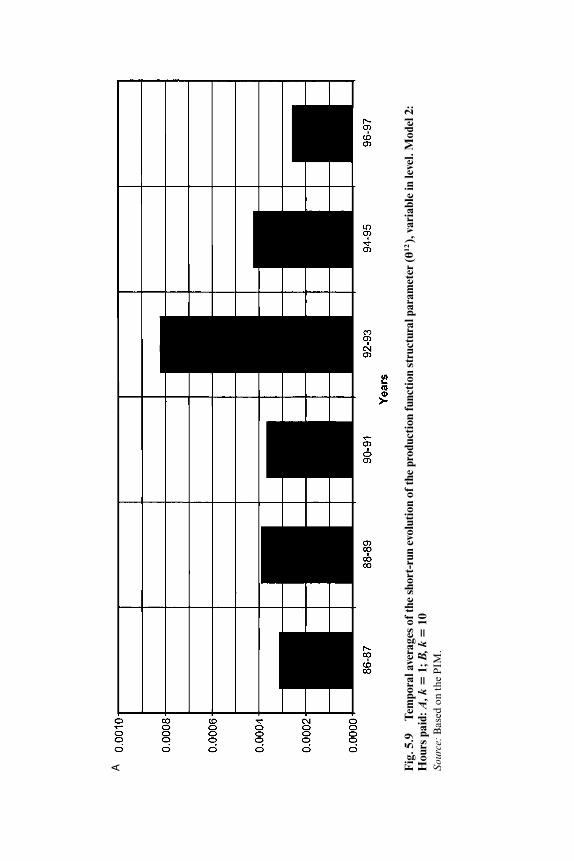
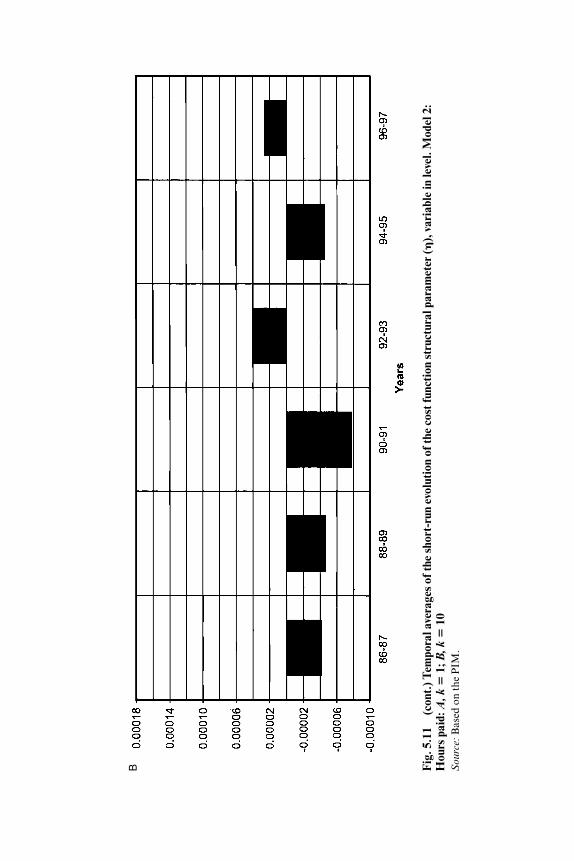
Basing our information on two-year averages of the temporal evolutionof these parameters and the values chosen for � and �, we obtain estimatesfor some important remaining structural parameters of the model: �12 and. These estimates are presented in figures 5.8, 5.9, 5.10, and 5.11.

Figures 5.2, 5.3, 5.6, and 5.7 provide clear evidence that both employ-ment and hours paid decline as labor costs rise. These figures, however,provide no clear evidence that either the short- or long-run response of em-ployment to labor costs increased as a consequence of the 1988 constitu-tional change.

Figures 5.4 and 5.5 give no evidence that the speed of adjustment wassignificantly affected by the 1988 constitutional change. In fact, figures 5.4and 5.5 reveal a modest continuous increase in the speed of adjustment,contrary to what would be expected from a discrete increase in firing costs.It is worth mentioning, however, that the estimates for have the correctsigned and are statistically significant, at least when we use the number ofemployed workers as a measure of the labor input. These estimates, how-ever, are considerably smaller (estimates for are around 0.5) than what iscommonly obtained from time series studies. Although the same pattern isobserved when we use the number of hours paid, some point estimates be-came negative, and it becomes considerably less precise. Finally, figures 5.4and 5.5 reveal that, as we choose instruments further into the past (i.e., ask increases), the estimated values for declines, indicating that serial cor-relation among technological shocks may seriously bias upwards.

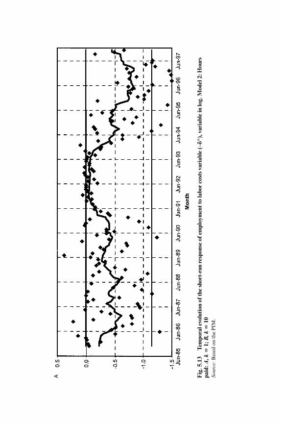
The interpretation of the basic parameters would be much easier if allvariables were in logs. The specification with all variables in logs is alsomore similar, related to the tradition in labor demand models. For thesereasons, we reestimate all previous models, changing all variables from lev-els to logs. Figures 5.12 to 5.17 show that the main results are robust to thelog specification.

As in the basic model, these figures provide no clear evidence that the1988 constitutional change had any significant impact on either the mag-nitude or the speed of the response of labor inputs to labor costs. These fig-ures deserve a few additional comments. First, they show that the short-and long-term wage elasticities are around –0.2 and –0.4, respectively.Second, it is worth mentioning that the estimates for the coefficient on lagof employment remain very close to 0.5, as is the case in the basic model.Third, it should be noted that the further the instruments are in the past,the smaller the estimated coefficients on lag employment, another patterncommon to the basic model.

To summarize the evidence about the effect of the 1988 constitutional


A Fig

. 5.6

Tem

pora

l evo

luti

on o

f the

long

-run

resp

onse

of e

mpl

oym

ent t

o la

bor

cost

s va

riab

le (–

ø), v

aria

ble

in le

vel.

Mod

el 1

: Em

ploy

men

tle

vel:

A,k

�1;

B,k

�10

Sou

rce:

Bas

ed o

n th

e P

IM.

B Fig

. 5.6

(con

t.) T

empo

ral e

volu

tion

of t

he lo

ng-r

un re

spon

se o

f em

ploy

men

t to

labo

r co

sts

vari

able

(–ø)

, var

iabl

e in

leve

l. M

odel

1: E

m-

ploy

men

t lev

el: A

,k�

1; B

,k�

10S

ourc

e:B

ased

on

the

PIM

.

A Fig

. 5.7

Tem

pora

l evo

luti

on o

f the

long

-run

resp

onse

of e

mpl

oym

ent t

o la

bor

cost

s va

riab

le (–

ø), v

aria

ble

in le

vel.

Mod

el 2

: Hou

rs p

aid:

A,k

�1;

B,k

�10

Sou

rce:

Bas

ed o

n th

e P

IM.

B Fig

. 5.7

(con

t.) T

empo

ral e

volu

tion

of t

he lo

ng-r

un re

spon

se o

f em

ploy

men

t to

labo

r co

sts

vari

able

(–ø)

, var

iabl

e in

leve

l. M

odel

2:

Hou

rs p

aid:

A,k

�1;

B,k

�10

Sou

rce:

Bas

ed o

n th

e P

IM.

A Fig

. 5.8

Tem

pora

l ave

rage

s of

the

shor

t-ru

n ev

olut

ion

of th

e pr

oduc

tion

func

tion

str

uctu

ral p

aram

eter

(�12

), v

aria

ble

in le

vel.

Mod

el 1

:E

mpl

oym

ent l

evel

: A,k

�1;

B,k

�10

Sou

rce:

Bas

ed o

n th

e P

IM.

B Fig

. 5.8

(con

t.) T

empo

ral a

vera

ges

of th

e sh

ort-

run

evol

utio

n of

the

prod

ucti

on fu

ncti

on s

truc

tura

l par

amet

er (�

12),

var

iabl

e in

leve

l. M

odel

1: E

mpl

oym

ent l

evel

: A,k

�1;

B,k

�10

Sou

rce:

Bas

ed o

n th

e P

IM.

A Fig

. 5.9

Tem

pora

l ave

rage

s of

the

shor

t-ru

n ev

olut

ion

of th

e pr

oduc

tion

func

tion

str

uctu

ral p

aram

eter

(�12

), v

aria

ble

in le

vel.

Mod

el 2

:H

ours

pai

d: A

,k�

1; B

,k�

10S

ourc

e:B

ased

on

the

PIM

.

B Fig

. 5.9

(con

t.) T

empo

ral a

vera

ges

of th

e sh

ort-

run

evol

utio

n of

the

prod

ucti

on fu

ncti

on s

truc

tura

l par

amet

er (�

12),

var

iabl

e in

leve

l. M

odel

2: H

ours

pai

d: A

,k�

1; B

,k�

10S

ourc

e:B

ased

on

the

PIM

.

A Fig

. 5.1

0T

empo

ral a

vera

ges

of th

e sh

ort-

run

evol

utio

n of

the

cost

func

tion

str

uctu

ral p

aram

eter

(�),

var

iabl

e in

leve

l. M

odel

1: E

mpl

oy-

men

t lev

el: A

,k�

1; B

,k�

10S

ourc

e:B

ased

on

PIM

.

B Fig

. 5.1

0(c

ont.

) Tem

pora

l ave

rage

s of

the

shor

t-ru

n ev

olut

ion

of th

e co

st fu

ncti

on s

truc

tura

l par

amet

er (�

), v

aria

ble

in le

vel.

Mod

el 1

: Em

-pl

oym

ent l

evel

: A,k

�1;

B,k

�10

Sou

rce:

Bas

ed o

n P

IM.

A Fig

. 5.1

1T

empo

ral a

vera

ges

of th

e sh

ort-

run

evol

utio

n of

the

cost

func

tion

str

uctu

ral p

aram

eter

(�),

var

iabl

e in

leve

l. M

odel

2: H

ours

pai

d:A

,k�

1; B

,k�

10S

ourc

e:B

ased

on

the

PIM

.

B Fig

. 5.1

1(c

ont.

) Tem

pora

l ave

rage

s of

the

shor

t-ru

n ev

olut

ion

of th

e co

st fu

ncti

on s

truc

tura

l par

amet

er (�

), v

aria

ble

in le

vel.

Mod

el 2

:H

ours

pai

d: A

,k�

1; B

,k�

10S

ourc

e:B

ased

on

the

PIM

.

A Fig

. 5.1

2T

empo

ral e

volu

tion

of t

he s

hort

-run

resp

onse

of e

mpl

oym

ent t

o la

bor

cost

s va

riab

le (–

�∗ )

, var

iabl

e in

log.

Mod

el 1

: Em

ploy

-m

ent l

evel

: A,k

�1;

B,k

�10

Sou

rce:

Bas

ed o

n th

e P

IM.

B Fig

. 5.1

2(c

ont.

) Tem

pora

l evo

luti

on o

f the

sho

rt-r

un re

spon

se o

f em

ploy

men

t to

labo

r co

sts

vari

able

(–�

∗ ), v

aria

ble

in lo

g. M

odel

1:

Em

ploy

men

t lev

el: A

,k�

1; B

,k�

10S

ourc

e:B

ased

on

the

PIM

.

A Fig

. 5.1

3T

empo

ral e

volu

tion

of t

he s

hort

-run

resp

onse

of e

mpl

oym

ent t

o la

bor

cost

s va

riab

le (–

�∗ )

, var

iabl

e in

log.

Mod

el 2

: Hou

rspa

id: A

,k�

1; B

,k�

10S

ourc

e:B

ased

on

the

PIM

.

B Fig

. 5.1

3(c

ont.

) Tem

pora

l evo

luti

on o

f the

sho

rt-r

un re

spon

se o

f em

ploy

men

t to

labo

r co

sts

vari

able

(–�

∗ ), v

aria

ble

in lo

g. M

odel

2:

Hou

rs p

aid:

A,k

�1;

B,k

�10

Sou

rce:

Bas

ed o

n th

e P

IM.

A Fig

. 5.1

4T

empo

ral e

volu

tion

of t

he s

hort

-run

resp

onse

of e

mpl

oym

ent t

o la

gged

em

ploy

men

t var

iabl

e (�

), v

aria

ble

in lo

g. M

odel

1:

Em

ploy

men

t lev

el: A

,k�

1; B

,k�

10S

ourc

e:B

ased

on

the

PIM

.

B Fig

. 5.1

4(c

ont.

) Tem

pora

l evo

luti

on o

f the

sho

rt-r

un re

spon

se o

f em

ploy

men

t to

lagg

ed e

mpl

oym

ent v

aria

ble

(�),

var

iabl

e in

log.

Mod

el1:

Em

ploy

men

t lev

el: A

,k�

1; B

,k�

10S

ourc

e:B

ased

on

the

PIM

.

A Fig

. 5.1

5T

empo

ral e

volu

tion

of t

he s

hort

-run

resp

onse

of e

mpl

oym

ent t

o la

gged

em

ploy

men

t var

iabl

e (�

), v

aria

ble

in lo

g. M

odel

2:

Hou

rs p

aid:

A,k

�1;

B,k

�10

Sou

rce:

Bas

ed o

n th

e P

IM.

B Fig

. 5.1

5(c

ont.

) Tem

pora

l evo

luti

on o

f the

sho

rt-r

un re

spon

se o

f em

ploy

men

t to

lagg

ed e

mpl

oym

ent v

aria

ble

(�),

var

iabl

e in

log.

Mod

el2:

Hou

rs p

aid:

A,k

�1;

B,k

�10

Sou

rce:

Bas

ed o

n th

e P

IM.

A Fig

. 5.1

6T

empo

ral e

volu

tion

of t

he lo

ng-r

un re

spon

se o

f em

ploy

men

t to

labo

r co

sts

vari

able

(–ø)

, var

iabl

e in

log.

Mod

el 1

: Em

ploy

men

tle

vel:

A,k

�1;

B,k

�10

Sou

rce:

Bas

ed o

n th

e P

IM.

B Fig

. 5.1

6(c

ont.

) Tem

pora

l evo

luti

on o

f the

long

-run

resp

onse

of e

mpl

oym

ent t

o la

bor

cost

s va

riab

le (–

ø), v

aria

ble

in lo

g. M

odel

1: E

m-

ploy

men

t lev

el: A

,k�

1; B

,k�

10S

ourc

e:B

ased

on

the

PIM

.

A Fig

. 5.1

7T

empo

ral e

volu

tion

of t

he lo

ng-r

un re

spon

se o

f em

ploy

men

t to

labo

r co

sts

vari

able

(–ø)

, var

iabl

e in

log.

Mod

el 2

: Hou

rs p

aid:

A,k

�1;

B,k

�10

Sou

rce:

Bas

ed o

n th

e P

IM.

B Fig

. 5.1

7(c

ont.

) Tem

pora

l evo

luti

on o

f the

long

-run

resp

onse

of e

mpl

oym

ent t

o la

bor

cost

s va

riab

le (–

ø), v

aria

ble

in lo

g. M

odel

2:

Hou

rs p

aid:

A,k

�1;

B,k

�10

Sou

rce:

Bas

ed o

n th

e P

IM.

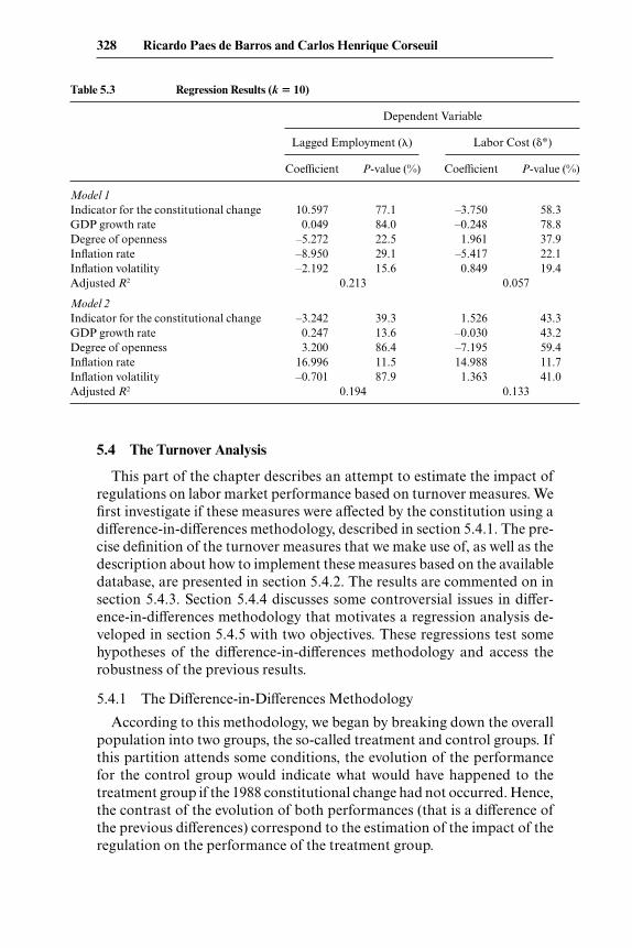
change on labor demand, we regress18 monthly estimates of the parameters and �∗ on an indicator for the constitutional change and control for a setof basic macroeconomic variables. These regressions also include monthlydummies and a linear trend. The results are presented in tables 5.2 and 5.3.

If the constitutional change actually increases labor costs and, as a con-sequence, has an important effect on the demand for labor, then the esti-mated coefficients for the indicator of constitutional change would be posi-tive and statistically significant in the regressions involving both parameters.This would be the case because an increase in variable labor costs would in-crease � and hence �∗, whereas an increase in firing costs would increasethe cost of adjustment and reduce the speed of adjustment leading to an in-crease in .

Contrary to these expected results, in the regressions presented in tables5.2 and 5.3 we found no evidence indicating that the 1988 constitutionchange had any significant effect on the labor demand function. All esti-mates of the constitution indicator coefficient are not statistically signifi-cant, despite the regression R2 reach values close to 0.4.


18. As demonstrated in section 5.3.3, in these regressions we used as our dependent vari-able the parameter estimate divided by its corresponding standard error. Our purpose was toreduce the influence of outliers. If the standard error was influenced by the constitutionalchanges, this procedure would generate biased estimates. But, as this is not the case, estimatesextracted from these same regressions, considering only the parameter as a dependent vari-able, leads us to the same conclusion about the lack of importance of constitutional changesfor the level of the parameter.

Table 5.2 Regression Results (k � 1)

Dependent Variable

Lagged Employment () Labor Cost (�∗)

Coefficient P-value (%) Coefficient P-value (%)

Model 1Indicator for the constitutional change –1.542 77.1 –1.861 58.3GDP growth rate –0.081 84.0 –0.069 78.8Degree of openness 8.617 22.5 –3.998 37.9Inflation rate 11.377 29.1 –8.461 22.1Inflation volatility 2.491 15.6 1.460 19.4Adjusted R2 0.358 0.026

Model 2Indicator for the constitutional change –5.578 39.3 2.320 43.3GDP growth rate 0.743 13.6 –0.177 43.2Degree of openness –1.499 86.4 –2.111 59.4Inflation rate 20.985 11.5 9.474 11.7Inflation volatility –0.329 87.9 –0.807 41.0Adjusted R2 0.135 0.065

5.4 The Turnover Analysis

This part of the chapter describes an attempt to estimate the impact ofregulations on labor market performance based on turnover measures. Wefirst investigate if these measures were affected by the constitution using adifference-in-differences methodology, described in section 5.4.1. The pre-cise definition of the turnover measures that we make use of, as well as thedescription about how to implement these measures based on the availabledatabase, are presented in section 5.4.2. The results are commented on insection 5.4.3. Section 5.4.4 discusses some controversial issues in differ-ence-in-differences methodology that motivates a regression analysis de-veloped in section 5.4.5 with two objectives. These regressions test somehypotheses of the difference-in-differences methodology and access therobustness of the previous results.

5.4.1 The Difference-in-Differences Methodology

According to this methodology, we began by breaking down the overallpopulation into two groups, the so-called treatment and control groups. Ifthis partition attends some conditions, the evolution of the performancefor the control group would indicate what would have happened to thetreatment group if the 1988 constitutional change had not occurred. Hence,the contrast of the evolution of both performances (that is a difference ofthe previous differences) correspond to the estimation of the impact of theregulation on the performance of the treatment group.


Table 5.3 Regression Results (k � 10)

Dependent Variable

Lagged Employment () Labor Cost (�∗)

Coefficient P-value (%) Coefficient P-value (%)

Model 1Indicator for the constitutional change 10.597 77.1 –3.750 58.3GDP growth rate 0.049 84.0 –0.248 78.8Degree of openness –5.272 22.5 1.961 37.9Inflation rate –8.950 29.1 –5.417 22.1Inflation volatility –2.192 15.6 0.849 19.4Adjusted R2 0.213 0.057

Model 2Indicator for the constitutional change –3.242 39.3 1.526 43.3GDP growth rate 0.247 13.6 –0.030 43.2Degree of openness 3.200 86.4 –7.195 59.4Inflation rate 16.996 11.5 14.988 11.7Inflation volatility –0.701 87.9 1.363 41.0Adjusted R2 0.194 0.133

Ideally, the treatment group would be the group most affected by thechange in legislation. The control group, on the other hand, ideally musthave two properties. First, contrary to the treatment group, it should notbe affected at all by the change in legislation. Second, the impact of theunderlying macroeconomic changes on the treatment and control groupsmust be very similar.

To implement this methodology, we use three alternative ways to breakdown the population in treatment and control groups.

Quits Versus Layoffs

Data regarding the informal sector is not always available. This is par-ticularly the case when administrative files are used. Hence, it is importantto identify other sources of cross-section variation in the legislation. Thedichotomy between quits and layoffs is one possibility.

In general, regulations involving quits are totally different from thoseregulating dismissals. In Brazil, quits remain essentially unregulated, whilea considerable amount of legislation was designed to restrict dismissalswithout just cause. Moreover, the changes brought by the new constitutionare entirely related to dismissals. They are silent with respect to quits.Hence, quits and layoffs correspond to our second alternative for the par-tition between treatment and control groups.

Short Versus Long Employment Spells

According to the new and previous constitutions, the entire regulationon dismissals without just cause only applies to employment spells thathave lasted at least three months. Dismissals of workers that have not yetcompleted three months on the job have been and still are completely un-regulated. Hence, an alternative partition in treatment and control groupscan be achieved through the contrast between very short spells (control)and other employment spells (treatment), where we consider as very shortspells all those that last less than three months.

Formal-Informal Dichotomy

According to the Brazilian labor laws all workers must have a documentnamed carteira de trabalho. This document, which resembles a little note-book or passport, acts as a complete record of the main parameters of theworker’s current, and all previous, formal labor contracts. In principle,whenever a worker’s labor contract is modified, either by moving to a newjob or by renegotiating his contract with his current employer, the mainparameters of the new contract must be immediately transcribed to theworker’s carteira de trabalho.

The existence of this document permits an easy empirical separation ofworkers with formal labor contracts that must comply with the labor lawsfrom workers with informal labor contracts that are not under this legisla-


tion. Workers with formal labor contracts are all employees who have theterms of their current labor contract transcribed to their carteira de tra-balho. Those whose employers have not registered their labor contract intheir carteira de trabalho should be considered informal.

This clear conceptual dichotomy would be of little practical relevance ifthe Brazilian employment surveys did not empirically investigate this ques-tion. Fortunately, however, essentially all household and employment sur-veys in Brazil do ask each employee in the sample whether their currentlabor contract is registered in their carteira de trabalho. As a result, it ispossible and easy to separate empirically the pool of employees accordingto whether they have or do not have a formal (registered in their carteira detrabalho) labor contract. Moreover, this dichotomy is of the utmost im-portance, because around 25 percent of the urban occupied labor force isemployed without a formal labor contract. So the formal and informal par-tition of the worker population corresponds to our first alternative of treat-ment (formal) and control (informal) groups.

5.4.2 Measuring Turnover Rates

Conceptual Preliminaries

As an indicator of turnover we use the probability that the employmentspell will be terminated next month, conditional on its current duration.This probability as a function of the current duration of the spell is com-monly referred as the hazard function. Evidently, in this case the indica-tor—the hazard function—is inversely related to the duration of employ-ment.

The hazard function is usually preferred to its complement, the proba-bility that it will not be terminated next month, conditional on its currentduration. In part, this preference derives from the fact that it can be bro-ken down according to the nature of the separation. In fact, if an employ-ment spell can only be terminated by a quit or dismissal, then the hazardfunction is equal to the sum of the probability that the employment spellwill be terminated by a quit and the corresponding probability that it willbe terminated by a dismissal, where both probabilities are conditional onthe current duration of the spell. The probability that an employment spellwill be terminated by a quit (dismissal), conditional on its current dura-tion, is commonly referred to as the transition intensity function. Hence, theproperty just stated can be summarized by saying that the hazard equals tothe sum of the transition intensities.

To define these measures precisely, some symbols must be introducedfirst. Accordingly, let �t be the universe of all active employment relation-ships at time t, and for each � in �t , let Dt(�) denote the incomplete dura-tion of the relationship � up to time t. Moreover, let St(�) denote an indi-cator of whether (S � 1) or not (S � 0) the relationship � will be terminated


in the month beginning at time t. The hazard rate, ht (d ), is then defined asthe probability that an active employment relationship, which up to time thas already lasted d months, will be terminated next month, that is,

ht(d ) � P(St � 1Dt � d ).

Moreover, let Qt(�) and Lt(�) be indicators of whether the relationship� will be terminated next month by a quit or a dismissal, respectively. Thequit and dismissal transition intensities can be expressed, respectively, by

htq (d ) � P (Qt � 1Dt � d )

and

h lt (d ) � P (Lt � 1Dt � d ).

If a separation can only occur due to a quit or a dismissal, then

ht (d ) � htq(d ) � h l

t (d ).

These equations refer to the probability of separation for employmentspells of a given duration in months. In practice, however, it is more con-venient to use the probability of separation for all employment spells withthe duration in any given interval.19 For instance, it may be more conven-ient to analyze the probability of separations of employment spells thathave already lasted six months but have not yet completed one year thanthe probability of separation of employment spells that have lasted up tonow exactly seven months. Fortunately, the above equations can easily beadapted to define the probability of separations for all employment spellswith the duration in any given interval. Resuming, we refer to these prob-abilities as the aggregated hazard and transition intensity rates.

To define them precisely, let {ai : i � 1, . . . , z} be a partition of N � {0,1, . . .}, so that

ai � {di , . . . , di�1}

for all i � 1, . . . , z, 0 � d1 � d2 � . . . � dz , and az � {dz , dz�1, . . .}. More-over, let Hti denote the probability that an active employment relationshipthat up to time t has already lasted between di and di�1 months will be ter-minated next month. Then Hti is given by

Hti � P (St � 1di � Dt � di�1) � P (St � 1Dt ∈ ai ).

By analogy we can define the corresponding transition intensities, respec-tively, by

(7) Hqti � P (Qt � 1di � Dt � di�1) � P (Qt � 1Dt ∈ ai )


19. Conceptually, d should refer to an instantaneous measure of time. In this sense the useof month is already a simplification for practical purposes.

and

Hlti � P (Lt � 1di � Dt � di�1) � P (Lt � 1Dt ∈ ai ).

In this study we divide employment spells according to their duration infour intervals; that is, we consider the case n � 5. These five intervals aredetermined by choosing d1 � 0, d2 � 3, d3 � 6, d4 � 12, d5 � 24. Hence,spells in the first interval are those that have not yet lasted three months.To simplify the exposition, we refer to them as the very-short spells. Thesecond interval consists of all spells that have already lasted at least threemonths but have not yet reached six months. Spells in this interval are re-ferred to as the short spells. The third interval is made of all spells that havealready lasted at least six months but have not yet reached one year. Spellsin this interval are referred to as the not-so-short spells. The fourth inter-val is made of all spells that have already lasted at least one year but havenot yet reached two years. We are going to refer to them as the long spells.Finally, the fifth interval is made of all spells that have already lasted atleast two years. We are going to refer to them as the very-long spells.

To obtain estimates for hazard and transition intensities we combinethree distinct data sets: the Relação Annual de Informações Sociais (RAIS),the Cadastro Geral de Empregados e Desempregados (CAGED), and thePesquisa Mensal de Emprego (PME). The PME is a monthly employmentsurvey, while RAIS and CAGED are administrative files.20 Three alterna-tive empirical procedures are pursued to obtain consistent estimates of thetemporal evolution of these probabilities from these data sets. First, twocombine data from RAIS and CAGED, while the other relies exclusivelyon PME data. The data used as well as the nature of the hypothesis neces-sary to obtain consistent estimators vary considerably between these fourprocedures. We describe each one of the three empirical procedures in turnin the next subsection.

Measures for Hazard and Transition Intensities

Our first procedure to estimate the transition probabilities consists of us-ing the information from RAIS on the stock of active employment rela-tionships classified by their incomplete duration up to time t, December 31


20. The Relação Annual de Informações Sociais (RAIS) is an annual administrative file thatprovides, at December 31 every year, a complete list of all active employment relationships inthe formal sector. The file also includes extensive characteristics of workers and firms. One ofthe characteristics available for every worker in the file is how long he has been in the currentjob, that is, the worker’s tenure. Hence, based on this information, it is possible to estimate thedistribution of active employment relationships according to their incomplete duration up toDecember 31 of each year. The RAIS is available for all years from 1985 to 1996. The Cadas-tro Geral de Empregados e Desempregados (CAGED) is a monthly administrative file that pro-vides data on the formal sector of all separations that occurred in a given month. This file alsoincludes information about the nature of the separation and basic information on workersand firms. In particular, it is possible to identify in each separation the reason for the separa-tion (quits versus dismissals) and the complete duration of the employment spell.

of a given year, and from CAGED on (1) how many of these active em-ployment relationships are terminated in January of the following year;(2) how many are terminated by quits; and (3) how many are terminated bydismissals. The number of active employment relationships that at time thas already lasted d months is represented by Nt (d ), while the number cor-respondent to those terminated in January by Mt (d ). Those terminated byquits are represented by Mt

q(d ), and, finally, those terminated by dismissalsby Ml

t (d ). More specifically, we have

Nt (d ) � #(� in �tD (�) � d )

Mt (d ) � #(� in �tD (�) � d and S(�) � 1)

Mtq(d ) � #(� in �tD (�) � d and Q (�) � 1)

and

Mlt (d ) � #(� in �tD (�) � d and L(�) � 1).

Basing our information on this, we obtain the hazard and the transitionintensity functions for each year via

ht(d ) � �M

Nt

t

(

(

d

d

)

)�,

htq(d ) � �

M

Nt

tq

(

(

d

d

)

)�,

and

hlt (d ) � �

M

Nt

lt

(

(

d

d

)

)�.

These expressions provide a useful method for estimating the probabil-ity of separations of employment spells during some months. Due to thenature of the available data, t is always December 31 for any given year.Consequently, the month beginning at t is always January of the followingyear. Hence, all estimates will refer to the probability that a separation willoccur in January, conditional on the duration of employment spells up toDecember 31. Therefore, even though we label these estimates by the yearassociated with time t, they do not reflect the average for this year. Actu-ally, the estimates refer to January of the following years. Estimates for theaggregated hazard and transition intensities can also be obtained by

Hti � ,

Hqti � ,

∑di�1

s�diMt

q(s)��∑di�1

s�diNt (s)

∑di�1s�di

Mt(s)��∑di�1

s�diNt(s)


and

(8) Hlti � .

Combining data from CAGED and RAIS it is possible to estimate allthese transition probabilities for each year between 1986 and 1995.

As already mentioned, these estimates described previously refer only totransitions taking place in January. Because these probabilities may followa seasonal pattern during the year, it is important to verify to what extentour conclusions are sensitive to the choice of a reference month. Unfortu-nately, we cannot precisely compute these transition probabilities for eachmonth because we only have data for the stock at December 31. Neverthe-less, an approximation of the average over the year can be obtained. In fact,because flows are observed for all months, we can combine the averagemonthly flow for the year with the stock at December 31 in order to obtainan approximation for average monthly transition probabilities for the year.Estimates of the aggregated hazard rate can be obtained by

H�ti � .

Once more combining data from CAGED and RAIS, it is possible to es-timate all these transition probabilities for each year between 1986 and1995.

We can also use data from PME to estimate transition probabilities forthe formal and informal sectors. PME is a typical employment survey cov-ering the six major Brazilian metropolitan areas. For this study we usemonthly data from this survey covering the period 1982–1997. The impor-tant feature of this survey is the fact that it has information on the completeduration of previous employment spells for those currently unemployed. Thesurvey also has information on whether these employment spells ended asquits or layoffs.

To obtain estimates for the hazard and transition intensities out of em-ployment from this data source, we have to assume, in addition to thesteady state hypothesis, that the duration of employment and unemploy-ment spells are stochastically independent. In this case, we can show (seeappendix B) that the aggregated hazard rate can be approximated by thefollowing equation:

Hti ≈ ,

�(di�1

1

� di )�∑di�1

s�diU l

t(s)

��

∑�

s�diUt (s) � �

1

2�∑ di�1

s�diUt(s)

�1

1

2� ∑11

i�0∑di�1s�di

Mt�i (s)��

∑di�1s�di

Nt(s)

∑di�1

s�diMt

l(s)��∑di�1

s�diNt (s)


where Ut(s) defines the number of unemployed workers at time t whose pre-vious job lasted a period contained in the interval denoted by s. Similarequations help estimate the aggregated transition intensities.

5.4.3 Empirical Results

To implement the difference-in-differences methodology we must specifya period before and after 1988. For a pre-1988 period we use the years 1986–1987. The choice of a post-1988 period is more difficult. We would like topick a period as close to 1988 as possible. On one hand, this choice wouldbe useful to isolate the effect of the drastic change in the constitution fromthe impact of other concomitant macroeconomic changes that occurredspread out over time. In other words, the closer the pre- and post-1988 pe-riods, the better for separating the impact of the constitutional change fromthe impact of changes in the macroeconomic environment. On the otherhand, because the effects of the 1988 constitutional change may also bespread out over time, capturing a significant portion of them would benecessary to use them for a post-1988 period, a time not very close to 1988.In the latter case, however, there would be no guarantee that the effect ofchanges in the macroeconomic environment was properly separated. Byvirtue of this trade-off, we choose the years 1991–1992 to represent the post-1988 period.

Estimates of the contrast between the aggregate hazard rates related tothese two periods are given in table 5.4. The estimates in this table indicatethat the hazard rate, mainly for short spells, dropped considerably just af-ter the constitutional change. The values stay around 2 percentage pointsfor this group.

Because the underlying macroeconomic environment did not remainconstant over this period, this finding should be taken with caution. In or-der to achieve a more precise result, we have to contrast the temporal differ-ence of the hazard rates associated with the treatment and control groups.

To describe the methodology more explicitly, let Y r0 and Y r

1 be an indi-cator of the duration of employment for the treatment group before and af-ter the constitutional change, respectively. Moreover, let Yc

0 and Yc1 be the


Table 5.4 First Differences of Hazard Rates: (1991/92)–(1986/87)

1/4–1/2 year 1/2–1 year 1–2 years

Administrative filesRais and caged (January flows) –2.7 –0.3 –0.3Rais and caged (average flows) –2.0 –0.5 –0.2

Employment surveyFormal –1.7 –0.7 –0.1Informal –0.8 –0.3 0.0

Sources: Based on the RAIS, CAGED, and PME.

corresponding indicator of the duration of employment for the controlgroup before and after the constitutional change, respectively. In the lattercase, the impact of the constitutional change on the treatment group willbe estimated by the difference-in-differences estimator, �, given by

� � (Y r1 � Y r

0) � (Yc1 � Yc

0 ).

To implement this methodology, we use three alternative ways to break-down the population in treatment and control groups. First, we use infor-mal workers as the control group and formal workers as the treatmentgroup. Second, we divide job separations into quits and dismissals. In thiscase, quits form the control group and dismissals the treatment group. Fi-nally, we use the very-short spells as a control group.

The decision about when to use each of these alternative control andtreatment groups was finally totally guided by data availability. In fact, weuse every alternative that the available data permitted us to use.

When quits are used as controls, the equation for this estimator is simpler.To arrive at this result, we should first notice that the response of quits tomacroeconomic changes behaves contrary to dismissals. In fact, as theeconomy moves into a recession, layoffs will increase while quits fall.Hence, when taking difference-in-differences we should change the sign ofthe first difference in quits before taking the second difference. More specif-ically, in this case the difference-in-differences estimator, �, is given by

� � (Yl1 � Yl

0 ) � (Yq1 � Yq

0 )

or the equivalent

� � (Yl1 � Yq

1) � (Yl0 � Yq

0 )

because, in general, Y l1 � Yq

1 � Y1 and Y l0 � Yq

0 � Y0 , where Y0 and Y1 arethe corresponding indicator for all separations before and after the consti-tutional change, respectively. It follows that in this case � � Y1 – Y0 , whichis the simple difference estimator investigated in the previous section. Inother words, all results presented in table 5.4 could be interpreted as beingobtained from the difference-in-differences estimator that use quits as acontrol group.

Table 5.5 presents difference-in-differences estimates for the impact ofthe constitutional change on employment duration, using the informal sec-tor and very-short spells as control groups.

When the informal sector is used as a control, at least for short spells, theestimated impact of the constitutional change on the duration of employ-ment is still negative and appreciable. The hazard rate for short spells de-clined in both the formal and informal sector from before to after the con-stitutional change, but the decline was 1 percentage point larger in theformal sector.

Table 5.5 also presents estimates using very-short spells as a control


group. The decline in the hazard rate for very-short spells was 0.5 to 1.5percentage point smaller than for short spells. However, when we comparethe evolution of the hazard rates for very-short spells with groups otherthan the short spells, we have opposite results with similar magnitude; thatis, the hazard rates for other spells were .5 to 1.5 percentage point smallerthan for very-short spells.

So the results seem to be easier to analyze by employment spell. We haveevidence that the hazard rates declined for short spell according to any ofthe three definitions implemented for the control group. No other employ-ment spells reported such a consistent pattern for hazard rates.

5.4.4 Some Limitations of the Methodology

Although changes in the legislation would not have a direct effect onthese control groups (one of the necessary conditions that the partition be-tween treatment and control has to attend), it is very likely that they wouldbe indirectly affected by the constitutional change. In section 5.2.2 we men-tion two mechanisms through which the constitution may affect quittingbehavior and the turnover among very-short duration spells. First, it is ar-gued that increases in dismissal penalties are likely to reduce quits as someworkers prefer to wait or even to force their dismissal in order to collect thecompensation, whereas according to the second argument, firms may in-crease the dismissal of employees before they complete three months onthe job in order to avoid the payment of dismissal penalties later.


Table 5.5 Differences-in-Differences of Hazard Rates: Treatment–Control

Database Dismissal–Quit Other Spells–Very Short Spell Formal–Informal

Rais and caged (January flows)

0–1/4 year –1.8 — —1/4–1/2 year –2.7 –0.9 —1/2–1 year –0.3 1.5 —1–2 years –0.3 1.5 —

Rais and caged (average flows)

0–1/4 year –0.8 — —1/4–1/2 year –2.0 –1.2 —1/2–1 year –0.5 0.3 —1–2 years –0.2 0.6 —

PME0–1/4 year –1.3 — 0.21/4–1/2 year –1.7 –0.5 –0.91/2–1 year –0.7 0.6 –0.41–2 years –0.1 1.2 0.0

Sources: Based on the RAIS, CAGED, and PME.Note: Dashes indicate that no calculations were implemented.

In addition to those arguments, there are also arguments that suggest theinformal sector may be indirectly affected by the constitution through atleast two channels. First, changes in the formal sector tend to affect the in-formal sector through its effects on overall labor market conditions, for in-stance, as a result of its effect on the unemployment rate. Second, changesin the legislation may play a role in the bargaining process even in the in-formal sector through their effect on the notion of fair labor relation.

There also exists another reason why the informal sector quits, and very-short spells may not be an ideal control group. Ideally, it is also necessarythat changes in the macroeconomic environment have identical impact onthe control and treatment groups. However, there is no theoretical or em-pirical reason why the response of quits and layoffs, short and long spells,and the formal and informal sectors to macroeconomic shocks should beof the same magnitude. Due to these limitations we decided to analyze re-sults from an alternative methodology.

5.4.5 Regression Analysis

The preceding empirical strategy requires data for only two periods intime: a pre- and a post-1988 period. However, if data is available for a largenumber of points in time and the macroeconomic changes can be charac-terized by measurable indicators, then it is possible to obtain estimates ofthe impact of the constitutional change and macroeconomic factors onhazard rates through a regression analysis.

The procedure would essentially consist of regressing monthly estimates(based on the PME) for the aggregated hazard rate on an indicator for theconstitutional change (i.e., an indicator that will have 0 as the value beforeand 1 as the value after the constitutional change), on another indicator forthe group (the treatment group is associated with the 0 value whether thecontrol group is associated with 1), on a set of macroeconomic indicatorsand interactions between the group indicator and each of the macroeco-nomic indicators, and also on the constitution indicator.

(9) ht,i (x1, x2, c, r) � 0 � x’1t � �1 � x’2t � �2 � 3 � ct � 4 � gi

� x’1t � �5 � gi � 6 � gi � ct � r’i � �7 � εti

x’1t is the transpose vector of values obtained for the four macroeconomicindicators in period t: a) the GDP real growth rate; b) the degree of open-ness as measured by the ratio between total trade (import plus exports) andthe GDP; c) the inflation rate; and d ) the volatility of the inflation rate asmeasured by its temporal standard deviation. x’2t is a transpose vector oftime invariant explanatory variables other than the constitutional indica-tor (ct). These variables are a linear time trend and monthly seasonal dum-mies. Regional indicator (r’i ) and group indicator (gi ) complement ourspecification. Finally, bold characters represent vector notation.


According to this framework the effect of constitution on the treatmentgroup can be written as 3. The estimation of this effect through regression(b3) will be a valid procedure even if the control group is affected by theconstitution or there are unbalanced macroeffects. On the other hand, theprocedure relies on the assumption that no other factor is related to hazardrates besides those considered in the regression framework.21

This procedure was done considering each one of the alternatives for thecontrol group and for each interval in turn, except for the very-short spell(this interval is never supposed to be affected by the constitution, evenwhen it is part of the treatment group). The estimated coefficients are re-ported on the upper part of tables 5.6, 5.7, and 5.8. The values associatedwith the constitutional indicator b3 are an alternative estimation for theimpact of the change in legislation on treatment groups’ turnover rates.The regression, however, adds an important information namely the confi-dence of the estimates.

We can see that from the nine alternative estimates of b3 (three employ-ment spells multiplied by three controls), four are significantly differentfrom zero. These significant coefficients are those associated with short andlong employment spells when either very-short spell or quit are used ascontrol. Among these four results we have two negative and two positiveestimates. The positive results correspond to those estimated for workerswhose employment spell is long, while negative results correspond to thoseestimated for workers whose employment spell is short. This last result isconsistent with findings in the last section.

The next step is the analysis of which control satisfies the necessary con-ditions stipulated for difference-in-differences estimators. Despite the factthat the test is based on a regression framework, the conditions are notnecessary for the regression estimators of the constitutional effects.

As already mentioned, for a control group to be considered valid, it mustsatisfy two properties. First, it must not be affected by the constitutionalchange. Second, macroeconomic changes must have the same impact onthe treatment and the control groups. As we described in section 5.4.4,those properties may not be valid for the control groups considered in thisstudy. However, both properties are testable under the assumption that wecan have explicit control for macroeconomic changes.

If the first property is valid (i.e., the constitutional change had no effecton the control group), then the expected value for the hazard rates associ-ated with the control group should be equal for periods before and after theconstitutional change. It can be precisely written as

Z � E(ht, i\gi � 1, ct � 1) � E(ht,i\gi � 1, ct � 0),


21. In fact, the regression would still produce valid results if those omitted factors affect inthe same way in both groups and the control is not affected by the constitution. In this caseour estimator of the effect of the constitution on the treatment group would be – 6.

Tab

le 5

.6P

oolin

g H

azar

d R

ates

for

the

Form

al a

nd I

nfor

mal

Sec

tors Sh

ort S

pell

Not

-So-

Shor

t Spe

llL

ong

Spel

l

Coe

ffici

ent

P-v

alue

(%)

Coe

ffici

ent

P-v

alue

(%)

Coe

ffici

ent

P-v

alue

(%)

Var

iabl

esIn

dica

tor

for

the

cons

titu

tion

al c

hang

e (b

3)0.

187

.50.

382

.9–1

.148

.6D

egre

e of

ope

nnes

s2.

31.

92.

012

.73.

55.

0G

DP

gro

wth

rat

e–1

2.0

0.9

–6.2

29.7

1.7

82.9

Infla

tion

vol

atili

ty0.

019

.40.

036

.90.

044

.9In

flati

on r

ate

1.0

50.9

–0.9

64.5

6.8

1.3

Indi

cato

r fo

r in

form

al s

ecto

r (b

4)–6

.40.

0–4

.31.

8–0

.874

.2b 4

�In

dica

tor

for

the

cons

titu

tion

al c

hang

e (b

6)–1

.330

.30.

098

.54.

35.

5b 4

�D

egre

e of

ope

nnes

s (b

51)

–1.2

36.2

0.8

63.0

–0.4

85.2

b 4�

GD

P g

row

th r

ate

(b52

)9.

81.

88.

611

.5–0

.792

.9b 4

�In

flati

on v

olat

ility

(b53

)0.

114

.10.

113

.90.

095

.7b 4

�In

flati

on r

ate

(b54

)–0

.389

.23.

718

.6–1

.766

.4

Tes

ts fo

r th

e va

lidit

y of

the

info

rmal

sec

tor

as c

ontr

ol g

roup

H1:

Inf

orm

al s

ecto

r no

t aff

ecte

d by

the

cons

titu

tion

(b3

�b 6

�0)

19.7

80.9

4.6

H2:

Eff

ects

of m

acro

econ

omic

indi

cato

rs a

re id

enti

cal i

n fo

rmal

an

d in

form

al s

ecto

r (b

51 �

b 52 �

b 53 �

b 54 �

0)5.

025

.499

.5

Sou

rce:

Bas

ed o

n th

e P

ME

.

Tab

le 5

.7P

oolin

g H

azar

d R

ates

for

the

Ver

y S

hort

and

Oth

er S

pells

Shor

t Spe

llN

ot-S

o-Sh

ort S

pell

Lon

g Sp

ell

Coe

ffici

ent

P-v

alue

(%)

Coe

ffici

ent

P-v

alue

(%)

Coe

ffici

ent

P-v

alue

(%)

Var

iabl

esIn

dica

tor

for

the

cons

titu

tion

al c

hang

e (b

3)–1

.02.

60.

357

.63.

30.

0D

egre

e of

ope

nnes

s2.

40.

03.

50.

03.

30.

0G

DP

gro

wth

rat

e–2

.724

.2–1

.367

.11.

178

.6In

flati

on v

olat

ility

0.0

15.9

0.0

4.8

0.0

12.2

Infla

tion

rat

e1.

212

.63.

30.

25.

00.

0In

dica

tor

for

very

sho

rt s

pell

(b4)

–5.6

0.0

–12.

10.

0–1

9.8

0.0

b 4�

Indi

cato

r fo

r th

e co

nsti

tuti

onal

cha

nge

(b6)

0.7

26.4

–0.7

44.6

–3.8

0.1

b 4�

Deg

ree

of o

penn

ess

(b51

)–0

.920

.5–1

.94.

1–2

.17.

0b 4

�G

DP

gro

wth

rat

e (b

52)

–4.3

4.2

–5.1

7.8

–6.8

6.2

b 4�

Infla

tion

vol

atili

ty (b

53)

0.0

86.5

0.0

63.9

0.1

5.2

b 4�

Infla

tion

rat

e (b

54)

–1.1

31.0

–3.3

3.1

–4.8

1.1

Tes

ts fo

r th

e va

lidit

y of

the

very

sho

rt s

pell

as c

ontr

ol g

roup

H1:

Ver

y sh

ort s

pell

not a

ffec

ted

by th

e co

nsti

tuti

on

(b3

�b 6

�0)

50.8

60.9

53.5

H2:

Eff

ects

of m

acro

econ

omic

indi

cato

rs a

re id

enti

cal i

n sh

ort a

nd v

ery

shor

t spe

lls (b

51 �

b 52 �

b 53 �

b 54 �

0)28

.47.

90.

7

Sou

rce:

Bas

ed o

n th

e P

ME

.N

ote:

Bas

ed o

n F

orm

al s

ecto

r.

Tab

le 5

.8P

oolin

g H

azar

d R

ates

for

the

Qui

t and

Dis

mis

sals

Sep

arat

ions

Shor

t Spe

llN

ot-S

o-Sh

ort S

pell

Lon

g Sp

ell

Coe

ffici

ent

P-v

alue

(%)

Coe

ffici

ent

P-v

alue

(%)

Coe

ffici

ent

P-v

alue

(%)

Var

iabl

esIn

dica

tor

for

the

cons

titu

tion

al c

hang

e (b

3)–1

.34.

5–0

.192

.72.

83.

0D

egre

e of

ope

nnes

s1.

81.

52.

81.

22.

67.

2G

DP

gro

wth

rat

e–2

.741

.4–1

.083

.44.

252

.4In

flati

on v

olat

ility

0.0

27.4

0.0

15.5

0.0

38.0

Infla

tion

rat

e1.

810

.34.

31.

06.

60.

3In

dica

tor

for

quit

sep

arat

ion

(b4)

–4.4

0.0

–6.2

0.0

–9.3

0.0

b 4�

Indi

cato

r fo

r th

e co

nsti

tuti

onal

cha

nge

(b6)

0.8

36.7

–1.8

18.3

–3.8

3.6

b 4�

Deg

ree

of o

penn

ess

(b51)

–3.1

0.2

–6.5

0.0

–8.8

0.0

b 4�

GD

P g

row

th r

ate

(b52)

–5.1

9.1

–4.5

31.3

–10.

58.

0b 4

�In

flati

on v

olat

ility

(b53)

–0.1

5.6

0.0

27.0

0.0

93.1

b 4�

Infla

tion

rat

e (b

54)

0.9

55.7

–0.2

91.6

–2.0

51.8

Tes

ts fo

r th

e va

lidit

y of

the

quit

sep

arat

ions

as

cont

rol g

roup

H1:

Qui

t not

aff

ecte

d by

the

cons

titu

tion

(b3

�b 6

�0)

46.9

5.0

43.3

H2:

Eff

ects

of m

acro

econ

omic

indi

cato

rs a

re o

ppos

ite

in q

uit

and

dism

issa

ls (–

b 11 �

2b51

; –b 12

�2b

52; –

b 13 �

2b53

; –b 14

�2b

54)

0.4

0.2

0.0

Sou

rce:

Bas

ed o

n th

e P

ME

.

where according to (9) we can see that22

Z � 3 � 6 .

Our statistic test will be based on the analogous estimated coefficients,

b3 � b6 ,

where we denoted as b the estimations of the true coefficients. So we havethat if the constitutional change did not affect the control group, the sumof the coefficient on the indicator for the constitutional change and the co-efficient on the interaction between the constitution and group indicatorsmust be zero.

If the second property is valid (i.e., macroeconomic changes have thesame effect on the control and treatment groups), then the expected valuefor the effect of the macroeconomic indicators on the hazard rates associ-ated with the treatment and control groups must be equal. It can be pre-cisely written as

E��∂∂x

ht

’1

,

t

i� \gi � 1� � E��

∂∂x

ht

’1

,

t

i� \gi � 0�,

which is equivalent to see if �5 � 0.23

Once more we will base our statistic tests on the analogous vector of es-timated coefficients (b5) to see if each of the elements of this vector is null(b1

5 � b25 � b3

5 � b45 � 0). This test is different when we consider quit as the

control. In this case we test if the effect of macroeconomic changes for bothgroups (quit and dismissals) had the same magnitude but opposite signs,that is,

E��∂∂h

xt

’1

,

t

i� \gi � 1� � � E��

∂∂h

xt

’1

,

t

i�\gi � 0�,

which is equivalent to see if –�5 � 2�1.The p-value related to both statistics tests mentioned previously, for each

of the nine regressions, is shown on the bottom part of tables 5.6, 5.7, and5.8. The results related to whether the control was affected by the constitu-tion are mostly in accordance with the null hypothesis of a null effect. Onlyone of the nine alternative combinations of control groups and employ-ment spells considered presents any evidence that it was affected by theconstitution—the informal workers whose duration spells are long. So


22. E(ht,i\gi � 1, ct � 1) � 0 � E(x’1i � �1\gi � 1, ct � 1) � E(x’2t � �2\gi � 1, ct � 1) � 3 � 4 � E(x’1t � �5\gi � 1, ct � 1) � 6 and E(ht,i\gi � 1, ct � 0) � 0 � E(x’2t � �1\ gi � 1, ct � 1) �E(x’2t � �2\gi � 1, ct � 1) � 4 � E(x’1t � �5\gi � 1, ct � 1).

23. According to equation (9) we have

E��∂xh

’1

t

t

,i� \gi � 1� � �1 � �5 and E��

∂xh

’1

t

t

,i� \ gi � 0� � �1.

there is almost no evidence of any effect of the constitution change on theinformal sector, the very-short employment spell, or quitting behavior.

However, when we consider whether the groups were equally affected byfactors other than the constitution, the results are not so favorable. Thishypothesis (considering the sign correction) was rejected among quit anddismissal separations. It was not rejected for the formal and informal par-tition, and for the very-short and other spells it was rejected only for thoseworkers whose employment spell was long.

So the best alternative to implementing the difference-in-differencesmethodology requires the use of the very-short spell or the informal sectoras control groups restricted to short and not-so-short employment spells.

5.5 Final Considerations

This study is an attempt to estimate the impact on the Brazilian labormarket performance due to the 1988 constitutional change. As a result ofthis change, the compensation for dismissals without just cause increasedfourfold. We investigate the impact of these changes on the parameters ofthe demand for labor and on hazard rates. If the constitutional change hada major impact, we should observe an important change in labor demandparameters and hazard rates around 1988.

Figures 5.2 and 5.3, however, provide no evidence at all that the consti-tutional change had any effect on labor demand parameters. Nevertheless,these figures reveal considerable temporal fluctuations in the coefficientsthat could be explained by macroeconomic events. To verify this possibil-ity, we regress our monthly estimates for the parameters of the demandfunction on an indicator for the constitution change and a series of macro-economic indicators. The results presented in tables 5.2 and 5.3 reveal thateven when taking into account macroeconomic variables, we still found noevidence that the 1988 constitution had any effect on the demand for labor.

Naturally, the fact that we were unable to find significant effects does notnecessarily imply that they do not exist. Our results are limited by the rich-ness and quality of our data and economic models. Much further researchis still necessary to reach a definite conclusion that labor demand dynam-ics were not very responsive to this constitutional change.

The estimations using hazard rates show ambiguous results. Accordingto difference-in-differences methodology (applied to appropriated controls),this turnover measure has declined for short employment spells (three tosix months) but seems to have increased for not-so-short employmentspells (six to twelve months). Regression analysis also provides ambiguousresults because it points to a decline for hazard rates associated with shortspells and an increase for long spells (twelve to twenty-four months).

Resuming, separation rates have decreased after the constitutionalchanges for the short employment spell and increased for longer spells,while parameters related to speed of adjustment and wage elasticity of em-


ployment have not changed. These facts may be consistent if the movementsregistered to separations in opposite directions cancel each other, keepingaggregate turnover and, consequently, the parameter mentioned un-changed.

There is a possible explanation for the movements on separation drivenby a combination of dismissals and quits movements. On one hand, firmsmight become more reluctant to fire a worker that did not fit the joboffered. They may then give more chances to see the worker perform ac-cording to what is expected. On the other hand, the accumulated amountof money on FGTS became more attractive to workers, and this attrac-tiveness increases with the employment spell. Hence, workers may have be-come more active in proposing a collusion with firms that he quits, pre-tending a firing and then having access to the fund. So if there is acorrespondence between the three- to six-month employment spell and thetime at which the firm became reluctant, and between longer employmentspells and the time at which worker tries the collusion, the results should bethose presented.

Appendix A

The Complete Derivation of the Structural Model for Labor Demand Shown in Section 5.2.1

In order to obtain an explicit solution to this problem of maximization, wementioned the introduction of a series of simplifying assumptions. Theseassumptions are described below.

First, we assume that the revenue function is separable in the followingsense:

R(ni (t), pi (t), �(t), �i (t)) � F (ni (t), �1(t)) � [G(pi(t), �

2(t)) � �i(t)]ni(t)

Under this assumption, the Euler equation associated with maximizingequation (1) is given by24

Fn(ni (t), �1(t)) � G(pi(t), �

2(t)) � � i(t) � �(t)wi (t) � C�(�ni (t), (t))

� �Et{C�(�ni(t � 1), (t � 1))} � 0.

We further simplify this model by assuming that the revenue function islinear-quadratic and the adjustment cost is quadratic; that is, we assumethat

F(ni (t), �1(t)) � �11(t)ni (t) �

�1

2

2(t)�ni (t)

2


24. We use Fn and C� to denote the derivatives of the F and ct functions in relation to theirfirst arguments.

and

C (�ni (t), (t)) � �

2

(t)� (�ni (t))

2,

where

�1(t) � (�11(t), �12(t)).

Furthermore, we assume that all firms in the same sector undergo thesame price of inputs. As a result,

G (pi (t), �2(t)) � ∑

m

s�1

ϕs(t)Iis ,

where Iis indicates whether firm i belongs to sector s, that is, Iis � 1 if firm ibelongs to sector s and Iis � 0 otherwise. Under these additional assump-tions the Euler equation becomes

��11(t) � �i (t) � ∑m

s�1

ϕs(t)Iis � �(t)wi (t)� � �12(t)ni (t) � (t)�ni(t)

� �(t){Et [ni (t � 1)] � ni(t)} � 0.

Under the assumption that parameters �12(t) and (t) are time invariantand that

Et��11(t � 1) � �i (t � 1) � ∑m

s�1

ϕs(t � 1)Iis � �(t � 1)wi (t � 1)�� 11(t) � �i (t) � ∑

m

s�1

ϕs(t)Iis � �(t)wi(t)�,

the solution of this equation is given by

ni (t) � ni (t � 1) � �(1

�

�12

)� ��11(t) � �i (t) � ∑

m

s�1

ϕs (t)Iis � �(t)wi(t)�as mentioned in section 5.2.1, where is implicitly defined by

�12 � (1 � )(1 � �).


Appendix B

Aggregate Hazard Rates and Transition Intensities Based on Employment Surveys, Steady-State Assumption, andStochastic Independence of Employment andUnemployment Spells

Let pt (d, u) represent the probability that a worker, whose previous joblasted d months and who is unemployed at time t for u months, will notleave the unemployment pool next month. Then, at each moment in timet, the number of unemployed workers whose previous jobs last d months,Ut(d ), is given by

Ut(d ) � ∑t

s��Ms(d )��

t�1

r�s

pr (d, r � s)��.

The steady state assumption implies that the time subscripts are not rel-evant. Thus, in particular, this equation can be rewritten as

U(d ) � M(d ) ∑�

s��

�

r�s

p(d, r � s)��.

Moreover, the stochastic independence of the duration of the employ-ment and unemployment spells implies that

p(d, r � s) � (r � s).

Therefore,

U(d ) � M(d ) ∑�

s��

�

r�s

(r � s�� ΛM(d ),

where

Λ � ∑�

s��

�

r�s

(r � s��.

Hence, we have established the useful result that at each moment in timethe number of unemployed workers whose previous jobs lasted d months,Ut(d ), is proportional to the number of employment spells of duration dending at time t, Mt(d ).

From steady-state assumption it is possible to write the hazard rate as afunction of the separations as shown in the following expression:

ht(d ) � �M

Nt

t

(

(

d

d

)

)� � � ,

where we used the assumption that all employment spells have finite dura-tion to obtain that limd→�Nt(d ) � 0, which implies in

Mt(d )��∑�

s�d Mt(s)

Mt(d )��

�Nt(0) � ∑s�0d�1 Mt (s)�


Nt(0) � ∑�

s�0

Mt(s).

Therefore, the hazard rate can be obtained from the data on unemployedworkers by

ht(d ) � � .

If it is also assumed that the duration of the unemployment spell is inde-pendent of whether the previous employment spell ended by a quit or dis-missal, then the transition intensities could also be obtained from data onunemployment workers by

qt(d ) �

and

lt (d ) � ,

where Utq(d ) is the number of unemployed workers at time t whose previ-

ous job lasted d months and ended in a quit, and U lt (d ) is the number of un-

employed workers at time t whose previous jobs lasted d months and endedin a dismissal.

We take similar steps to write the aggregate hazard rates that can be writ-ten as

Hti �

to the extent that

is very small.

∑di�1

s�di

∑�

r�1

Mt(r) ≈ (di�1 � di )�∑�

s�di�1

Mt(s) � �1

2� ∑

di�1

s�di

Mt(s)�That allows us to simplify the expression for the aggregates hazard rate to

Hti ≈ .

�(di�1

1

� di )� ∑di

s�diMt(s)

��

∑�

s�di�1Mt(s) � �

1

2� ∑ s�di

di�1 Mt(s)

∑di�1s�di

Mt(s)��∑�

s�diMt(s)

∑di�1s�di

Mt(s)��∑di�1

s�di ∑�

r�s Mt(r)

U 1t (d )

��∑ �

s�d U 1t (s)

Utq(d )

��∑�

s�d Utq(s)

Ut(d )��∑�

s�d Ut (s)

Mt(d )��∑�

s�d Mt(s)


Considering that

Ut(d ) � ΛM(d ),

the aggregated hazard rate can be approximated by the following equation:

Hti ≈

References

Almeida, Sandra Cristina. 1992. As contribuições sociais de empregadores e tra-balhadores: Repercussões sobre o mercado de trabalho e grau de evasão. IPEAPolicy Document no. 8. Rio de Janeiro, Brazil: Institute for Applied EconomicResearch.

Almeida, Wanderly J. M. de, and José Luiz Chautard. 1976. FGTS: Uma políticade bemestar social. IPEA/INPES Research Report no. 30. Rio de Janeiro, Brazil:Institute for Applied Economic Research.

Amadeo, Edward, Ricardo Paes de Barros, José Márcio Camargo, and RosaneMendonça. 1995. Brazil. In Reforming the labor market in a liberalized economy,ed. Gustavo Márquez, 35–78. Washington, D.C.: Inter-American DevelopmentBank.

Amadeo, Edward, and José Márcio Camargo. 1993. Labour legislation and insti-tutional aspects of the Brazilian labour market. Labour 7 (1): 321–54.

———. 1996. Instituições e o mercado de trabalho brasileiro. In Flexibilidade domercado de trabalho no Brasil, ed. José Márcio Camargo, 47–94. Rio de Janeiro,Brazil: FGV.

Bacha, Edmar Lisboa, Milton da Mata, and Ruy Lyrio Modenesi. 1972. Encargostrabalhistas e absorção de mão-de-obra: Uma interpretação do problema e seudebate. IPEA Research Report no. 12. Rio de Janeiro, Brazil: Institute for Ap-plied Economic Research.

Barros, Ricardo Paes de, Carlos H. Corseuil, and Mônica Bahia. 1999. Labor mar-ket regulation and the duration of employment in Brazil. Rio de Janeiro, Brazil:IPEA Discussion Paper no. 676. Rio de Janeiro, Brazil: Institute for AppliedEconomic Research.

Barros, Ricardo Paes de, Carlos H. Corseuil, and Miguel Foguel. 2001. Os incen-tivos adversos e a focalização dos programas de proteção ao trabalhador noBrasil. IPEA Discussion Paper no. 784. Rio de Janeiro, Brazil: Institute for Ap-plied Economic Research.

Barros, Ricardo Paes de, Carlos H. Corseuil, and Gustavo Gonzaga. 1999. Labormarket regulation and the demand for labor in Brazil. Rio de Janeiro, Brazil:IPEA Discussion Paper no. 656. Rio de Janeiro, Brazil: Institute for AppliedEconomic Research.

Camargo, José Márcio, and Edward Amadeo. 1990. Labour legislation and insti-tutional aspects of the Brazilian labour market. Discussion Paper no. 252. Riode Janeiro, Brazil: Pontificia Universidade Catolica.

�(di�1

1

� di )�∑ s�di

di�1 Ult(s)

��

∑�

s�diUt(s) � �

1

2� ∑ s�di

di�1 Ut(s)


Carvalho, Carlos Eduardo, and Maurício Mota Saboya Pinheiro. 1999. FGTS:Avaliação das propostas de reforma e extinção. Rio de Janeiro: IPEA DiscussionPaper no. 671. Rio de Janeiro, Brazil: Institute for Applied Economic Research.

Chadad, José Paulo Zeetano. 1993. Encargos sociais e emprego no Brasil. Discus-sion Paper. São Paulo, Brazil: FIPE, USP.

Hamermesh, Daniel. 1993. Labor demand. Princeton, N.J.: Princeton UniversityPress.

Hamermesh, Daniel, and Gerard A. Pfann. 1996. Adjustment costs in factor de-mand. Journal of Economic Literature 34:1264–92.

Jatobá, Jorge. 1994. Encargos sociais, custos da mão de obra e flexibilidade do mer-cado de trabalho no Brasil. In Conferência sobre regulamentação do mercado detrabalho no Brasil, ed. IPEA, 1–36. Rio de Janeiro, Brazil: Institute for AppliedEconomic Research.

Macedo, Roberto Bras Matos. 1985. Diferenciais de salários entre empresas pri-vadas e estatais no Brasil. Revista Brasileira de Economia 39 (4): 448–73.

———. 1993. Reforma da previdência social: Resenha e consolidação. In A prev-idência social e a reforma constitucional, ed. Brasil, Ministério da Previdência So-cial, 4–47. Brasília, Brazil: CEPAL.

Malaga, Guillermo Tomás. 1992. Dynamic labor demands: Cases of interest forBrazil. In Anais XV. Encontro Brasileiro de Econometria, 1992, Campos doJordão (SP). São Paulo: SBE.

Nascimento, Amauri Mascaro. 1993. Iniciação ao direito do trabalho, ed. SBE, 409–30. São Paulo, Brazil: Sociedade Brasileira de Econometria.

Nickell, S. J. 1986. Dynamic models of labour demand. In Handbook of labor eco-nomics, vol. 1, ed. Orley Ashenfelter and Richard Layard, 437–522. Amsterdam:Elsevier.

Pastore, José. 1994. Encargos sociais no Brasil e no exterior: uma avaliacao critica.São Paulo, Brazil: SEBRAE.

World Bank. 1991. Brazil: The Brazilian labor market in the 1980s. World Bank Re-port no. 9693-BR. Washington, D.C.: World Bank.


this pdf is a selection from a published volume from the national ... · carlos henrique corseuil...

Documents