three detecting indexes and five regularization techniques for ... · three detecting indexes and...

Three detecting indexes and five regularization techniques for degenerate scales in the BEM/BIEM

Jeng-Tzong Chen1,2, Shing-Kai Kao1 & Shyh-Rong Kuo1 1Department of Harbor and River Engineering, National Taiwan Ocean University, Taiwan 2Department of Mechanical and Mechatronic Engineering, National Taiwan Ocean University, Taiwan

Abstract

It is well known that BEM/BIEM results in degenerate scale for a two-dimensional Laplace problem subjected to the Dirichlet boundary condition. In this paper, we reviewed three indexes for detecting the degenerate scale in BEM/BIEM and five regularization techniques to ensure the unique solution, the hypersingular formulation rank promotion by adding the boundary flux equilibrium, CHEEF method, (direct BEMs), Fichera’s method (indirect BEM) and method of adding a rigid body mode. In the numerical implementation, the BEM program developed by the NTOU/MSV group is employed to see the validity of the above formulation. Finally, a general shape of a regular triangle is numerically implemented to check the uniqueness solution of BEM. Keywords: BEM, BIEM, degenerate scale, ill-conditioned.

1 Introduction

While the boundary integral equation method (BIEM) or the boundary element method (BEM) is used to solve engineering problems, rank deficiency or the non-unique solution occurs when the domain of the problem is a specific size. It is well known that BEM/BIEM results in a degenerate scale for a two-dimensional interior Laplace problem subjected to the Dirichlet boundary condition [1]. There are many related terminologies such as Gamma contour [2], logarithmic capacity [3], critical value [4, 5], conformal radius [6], transfinite

Boundary Elements and Other Mesh Reduction Methods XXXVI 191

www.witpress.com, ISSN 1743-355X (on-line) WIT Transactions on Modelling and Simulation, Vol 56, © 2013 WIT Press

doi:10.2495/BEM360171

diameter [7], Robin constant [8] and Chebichev constant [8]. Petrovsky [9] pointed out the paradox for the degenerate scale by using the maximum principle and the mean value theorem. Physically speaking, it is obvious and is physically realizable that symmetric loading cannot excite the anti-symmetric vibration mode. The reason is that no work can be done using the Betti’s law. We know that the BIE is derived from the Green’s third identity which is similar to the Betti’s law in the theory of structures. It is similar that a fundamental solution may contribute no work for a special domain with a degenerate scale. Mathematically speaking, the degenerate scale can be understood by the fact that there is a nontrivial boundary flux for the trivial boundary potential. One way to avoid this problem is by scaling. A simple case of a circle with radius 1 can be easily found from the literature [9]. Although scaling can avoid the appearance of degenerate scale in the original problem, the problem still exists and moves the critical situation to another size. In other words, the degenerate scale is not solved, and it is only shifted to a new scale. Therefore, searching an efficient method to solve the Dirichlet Laplace problem for all scales is not trivial. Chen et al. also revisited this problem and they used the singular value decomposition technique [10] and the Combined Helmholtz Exterior integral Equation Formulation method (CHEEF) [10] to promote the rank in the boundary element method (BEM) and to obtain a unique solution. Recently, Chen and his coworkers analytically derived the degenerate scales of a circle [11], an elliptical case [12], a regular N-gon [13] and a semi-circular disc [14] through the unit logarithmic capacity by using the complex variable and numerically examined by using the BEM program. Kuo and Chen [15] linked the unit logarithmic capacity in the theory of complex variables and the degenerate scale in the BEM/BIEMs. It is known that the degenerate scale happens when the logarithmic capacity is equal to 1. This is a good index to judge where the degenerate scale occurs. Recently, Han et al. [17] provide another index to see the occurrence of the degenerate scale. Based on Fichera’s method [18] which was first provided by Fichera in 1961 [19], the method was developed by using the integral equation of first kind by adding a constant in the equation. Besides, it is also necessary to satisfy an extra constraint. Therefore, they provided a computable index with respect to the constant to judge where the degenerate scale happens. In this paper, we reviewed three indexes for detecting the degenerate scale in BEM/BIEM and five regularization techniques to ensure the unique solution. Finally, a general shape of a regular triangle is numerically implemented to check the uniqueness solution of BEM.

2 Three detecting indexes for the degenerate scale in the BEM/BIEM

The governing equation and boundary condition of the interior and exterior Laplace problem subject to the Dirichlet boundary condition are shown below:

192 Boundary Elements and Other Mesh Reduction Methods XXXVI


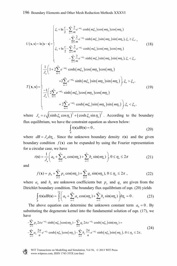
2 0, ,

( ), ,iu D

u f B

x x

x x x (1)

2 0, ,

( ), ,

is bounded, when ,

ou D

u f B

u

x x

x x x

x x

(2)

where 2 , iD , oD and B are the Laplacian operator, the interior bounded

domain, the exterior domain and the boundary, respectively. Single-layer representation for the solution yields the integral equations of the first kind as given below:

( , ) ( ) ( ) ( ),B

U dB f B s x s s x x , (3)

where the fundamental solution ( , ) ln .U s x x s In some case such as

the degenerate scale, we cannot obtain the solutions due to incompleteness for the representation of the solution by loss of a constant. Chen et al. [10] employed the SVD technique to find the ill-conditioned system due to the degenerate scale in the BEM. The influence matrix [ ]U in the SVD structure is

shown below:

TN N N N N N N NU

, (4)

where N N is a diagonal matrix and

1

2

N

0 0 0

0 0 0

0 0

N N

N N

. (5)

If the size is the degenerate scale such that 0U , 1 in the diagonal

matrix of eqn. (5) is equate to zero. The minimum singular value to be zero is the first index to detect the degenerate scale in BEM. Kuo and Chen [15] designed a null field of the degenerate scale to have a constant field for the interior domain, iD . They transformed the real-variable

BIE to the complex-variable BIE and let ( ) ( ) ( )G z u iv x x (6)

and ( ) , ,

( ) ( ) , ,i I i

o I

u C D

u f C B

x x

x x x (7)

where IC is a constant. Considering the Riemann conformal mapping from the

exterior circle in the w plane to the exterior domain bounded by B in the z plane, they have



1 21 0 2

....b b

z f w a w bw w

(8)

or

* *

* 1 21 0 2

....b b

z f w a w bw w

. (9)

Then they employed the indirect BEM to obtain

1

1

Re{ } ln ,Re{ ( )} ( , )

Re{ } Re{ln } ln ,

i i

o o

G z a z DG z x y

G z g z a z D

, (10)

where the subscripts of i and o denote the inner and outer domains of iD and

oD . The above equation indicates that the unit leading coefficient 1( 1)a of

the linear term in the Riemann conformal mapping of eqn. (8) results in an interior null field which matches well the BEM result once the degenerate scale happens. The leading coefficient of a1 is the second index in the theory of complex variables. Recently, Han et al. [17] employed Firchera’s technique to introduce a computable index for verifying the degenerate scale. To avoid the ill-

conditioned matrix of conventional indirect BEM, Fichera [18] proposed the boundary integral formulation as shown below:

( , ) ( ) ( ) ( ),B

U dB f B s x s s x x (11)

and a constraint equation

( ) ( ) 0B

dB s s , (12)

where ( ) s and are the unknown boundary density and an unknown real

constant, respectively. Han mark the boundary condition as

( ) ( , ) ( ),B

f U dB B x s x s x (13)

then

1( , ) ( , ) ( )

( ) B B B B

U dB dB U dB dBmeas B

s x s xs x s x s , (14)

where

( ) 1B

meas B dB s . (15)



If the size is the degenerate scale then of eqn. (14) is equate to zero. The

third index is derived from Fichera’s approach.

3 Five regularization techniques

Following the successful experiences of Chen et al. [19], we review and analytically derive the unique solution by using five regularization techniques (three techniques for the direct BEM, one technique for the indirect BEM and one modified technique for the kernel function) as shown in Table 1. For the analytical study, they employed the degenerate kernel in the polar and elliptic coordinates to derive the unique solution by using five regularization techniques for any size of circle and ellipse, respectively.

Table 1: Five regularization techniques for nonuniqueness in the BEM /BIEM.

Method Integral formulation Extra constraint

Fichera’s method ( , ) ( ) ( ) ( ),B

U dB f B s x s s x x ( ) ( ) 0B

dB s s

The boundary flux equilibrium

2 ( ) ( , ) ( ) ( )

( , ) ( ) ( ),

B

B

u T u dB

U t dB D

x s x s s

s x s s x

( ) ( ) 0B

t dB s s

The CHEEF method

0 ( , ) ( ) ( )

( , ) ( ) ( ),

B

c

B

T u dB

U t dB D

s x s s

s x s s x

The hypersingular formulation

2 ( ) ( , ) ( ) ( )

( , ) ( ) ( ),

B

B

t M u dB

L t dB D

x s x s s

s x s s x

The method of adding a rigid body mode

( , ) lnU r s x

3.1 Three regularization techniques for the direct BEM

By using the singular formulation, we have the boundary integral equation,

2 ( ) ( , ) ( ) ( ) ( , ) ( ) ( ),B B

u T u dB U t dB D x s x s s s x s s x , (16)

where ( , )

( , )U

Tn

s

s xs x and

( )( )

ut

n

s

ss . Therefore, the null-field integral

equation yields

0 ( , ) ( ) ( ) ( , ) ( ) ( ), c

B B

T u dB U t dB D s x s s s x s s x , (17)

where cD is the complementary domain. By setting the field point ( , ) x xx

and the source point ( , ) s ss , the fundamental solution by using the elliptic

coordinates can be expressed by using the following degenerate kernel for the elliptic case,



1

1

1

1

2ln cosh cos cos

2

2sinh sin sin , ,

, ln2

ln cosh cos cos2

2sinh sin sin , ,

m

m

m

m

m

m

m

m

ce m m m

m

e m m mm

Uc

e m m mm

e m m mm

s

s

x

x

s x x s

x x s s x

x s x s

s x s s x

x s x s,

(18)

1

1

1

1

11 2 cosh cos cos

2 sinh sin sin , ,

,1

2 sinh cos cos

2 cosh sin sin , ,

m

m

m

m

m

m

m

m

e m m mJ

e m m m

T

e m m mJ

e m m m

s

s

x

x

x x ss

x x s s x

s x ss

s x s s x

x s (19)

where 2 2sinh cos cosh sinJ c s s s s s . According to the boundary

flux equilibrium, we have the constraint equation as shown below:

( ) ( ) 0B

t dB s s , (20)

where dB J d s s . Since the unknown boundary density ( )t s and the given

boundary condition ( )f x can be expanded by using the Fourier representation

for a circular case, we have

01 1

1( ) cos( ) sin( ) , 0 2n n

n n

t a a n b nJ

s s ss

s (21)

and

01 1

( ) cos( ) sin( ), 0 2n nn n

f p p n q n

x x xx , (22)

where na and nb are unknown coefficients but np and nq are given from the

Dirichlet boundary condition. The boundary flux equilibrium of eqn. (20) yields 2

01 10

( ) ( ) cos( ) sin( ) 0n nn nB

t dB a a n b n d

s s ss s . (23)

The above equation can determine the unknown constant term 0 0a . By

substituting the degenerate kernel into the fundamental solution of eqn. (17), we have

0 0

0 0

0 01 1

0 01 1

2 sinh cos( ) 2 cosh sin( )

2 2cosh cos sinh sin , 0 2 ,

n nn n

n n

n nn n

n n

p e n n q e n n

a e n n b e n nn n

x x

x x x

(24)



where 0 is the radial coordinate of the elliptic boundary. Therefore, all the

unknown coefficients are uniquely determined as follows:

0

0

0

0,

tanh ,

coth .

n n

n n

a

a n n p

b n n q

(25)

For the elliptic case, eqn. (17) alone yields the non-unique solution of 0a .

Instead of adding the boundary flux equilibrium, we can resort the null-field integral equation by collocating the point ex outside the domain (CHEEF idea)

to add an independent constraint. For the elliptic case, we collocate the exterior point cosh cos , sinh sin ,e e e e ec c x where 0.e By

substituting the degenerate kernel and ex into the fundamental solution of

eqn. (17), we have

0 01 1

0 0 01 1


2 22 ln cosh cos sinh sin ,

2

0 2 .

e e

e e

n nn e n e

n n

n ne n e n e

n n

e

p e n n q e n n

ca a e n n b e n n

n n

(26)

According to eqn. (24) and one constraint of eqn. (26), all the unknown coefficients are uniquely obtained as follows:

0

0

0

0,

tanh ,

coth .

n n

n n

a

a n n p

b n n q

(27)

By using the hypersingular formulation, we have the boundary integral equation,

2 ( ) ( , ) ( ) ( ) ( , ) ( ) ( ),B B

t M u dB L t dB D x s x s s s x s s x , (28)

where ( , )

( , )U

Ln

x

s xs x and

( , )( , )

UM

n n

x s

s xs x . Therefore, the null-field

integral equation yields

0 ( , ) ( ) ( ) ( , ) ( ) ( ), c

B B

M u dB L t dB D s x s s s x s s x . (29)

For the circular case, ( , )L s x and ( , )M s x can be expressed by using the

following degenerate kernels, respectively,



1

1

1

1

12 sinh cos cos

2 cosh sin sin , ,

,1

1 2 cosh cos cos

2 sinh sin sin ,

m

m

m

m

m

m

m

m

e m m mJ

e m m m

L

e m m mJ

e m m m

s

s

x

x

x x sx

x x s s x

s x sx

s x s s x

x s (30)

and

1

1

1

1

12 sinh cos cos

2 cosh sin sin , ,

,1

2 sinh cos cos

2 cosh sin sin , .

m

m

m

m

m

m

m

m

me m m mJ J

me m m m

M

me m m mJ J

me m m m

s

s

x

x

x x sx s

x x s s x

s x sx s

s x s s x

x s (31)

By substituting the degenerate kernel into the fundamental solution of eqn. (29), we have

0 0

0 0

0 01 1

0 0 01 1


2 12 cosh cos 2 sinh sin ,

0 2 .

n nn n

n n

n nn n

n n

p n e n n q n e n nJ

a a e n n b e n nJ J

x xx

x xx x

x

(32)

Therefore, all the unknown coefficients according to the hypersingular equation are uniquely obtained as follows:

0

0

0

0,

tanh ,

coth .

n n

n n

a

a n n p

b n n q

(33)

3.2 Regularization technique for indirect method

Single-layer representation for the solution yields the integral equations of the first kind as given below:

( , ) ( ) ( ) ( ),B

U dB f B s x s s x x . (34)



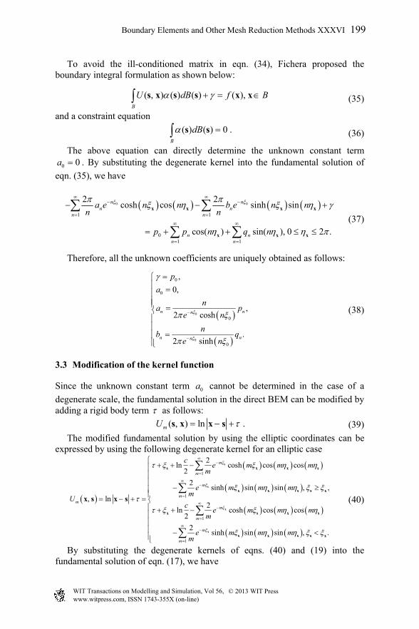
To avoid the ill-conditioned matrix in eqn. (34), Fichera proposed the boundary integral formulation as shown below:

( , ) ( ) ( ) ( ),B

U dB f B s x s s x x (35)

and a constraint equation

( ) ( ) 0B

dB s s . (36)

The above equation can directly determine the unknown constant term

0 0a . By substituting the degenerate kernel into the fundamental solution of

eqn. (35), we have

0 0

1 1

01 1

2 2cosh cos sinh sin

cos( ) sin( ), 0 2 .

n nn n

n n

n nn n

a e n n b e n nn n

p p n q n

x x x x

x x x

(37)

Therefore, all the unknown coefficients are uniquely obtained as follows:

0

0

0

0

0

0

,

0,

,2 cosh

.2 sinh

n nn

n nn

p

a

na p

e n

nb q

e n

(38)

3.3 Modification of the kernel function

Since the unknown constant term 0a cannot be determined in the case of a

degenerate scale, the fundamental solution in the direct BEM can be modified by adding a rigid body term as follows:

( , ) lnmU s x x s . (39)

The modified fundamental solution by using the elliptic coordinates can be expressed by using the following degenerate kernel for an elliptic case

1

1

1

1

2ln cosh cos cos

2

2sinh sin sin , ,

, ln2

ln cosh cos cos2

2sinh sin sin , .

m

m

m

mm

m

m

m

m

ce m m m

m

e m m mm

Uc

e m m mm

e m m mm

s

s

x

x

s x x s

x x s s x

x s x s

s x s s x

x s x s

(40)

By substituting the degenerate kernels of eqns. (40) and (19) into the fundamental solution of eqn. (17), we have



0 0

0 0

0 01 1

0 0 0 01 1


2 22 ln cosh cos sinh sin ,

2

0 2 .

n nn n

n n

n nn n

n n

p e n n q e n n

ca a e n n b e n n

n n

x x

x x

x

(41)


0

0

0

0,

tanh ,

coth .

n n

n n

a

a n n p

b n n q

(42)

Similarly, we substitute the degenerate kernel of eqn. (40) into the fundamental solution of eqn. (34) to obtain

0 00 0 0 0

1 1

01 1

2 22 ln cosh cos sinh sin

2

cos( ) sin( ),0 2 .

n nn n

n n

n nn n

ca a e n n b e n n

n n

p p n q n

x x

x x x

(43)


0

0

0 0

0

0

0

1

2 ln2

,2 cosh

.2 sinh

n nn

n nn

a pc

na p

e n

nb q

e n

(44)

It is noted that the original degenerate scale is avoided by adding a rigid body term but just move to another critical scale.

4 Numerical results and discussions

Here, we consider a regular triangle to examine the three detecting indexes and to see the validity of five regularization techniques to promote the linear algebraic system to be full rank. Singular values are not zeros for any scale size after regularization as shown in Table 1. The five approaches except the method of adding a rigid body mode are valid for all sizes. The least method just moves the critical size to other size. For the general shape of a regular triangle, the degenerate scale appears when the side length is equal to 2.37105 which satisfies the analytical formula in [13]. Besides, three indexes 1 1, anda are found to

be effective in detecting the degenerate scale. Numerical results math well with analytical derivations as shown in Table 2.



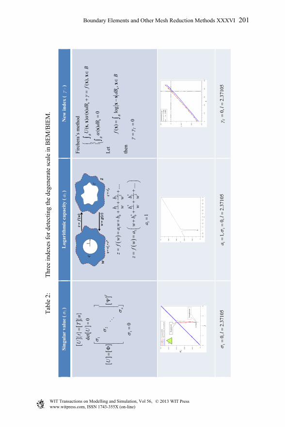
Tab

le 2

: T

hree

inde

xes

for

dete

ctin

g th

e de

gene

rate

sca

le in

BE

M/B

IEM

.

Sin

gula

r va

lue

( σ 1

) L

ogar

ith

mic

cap

acit

y(

a 1 )

New

inde

x ( γ

Γ )

U

tT

u

det

0U

1

2T

n

U

10

zw

()

zf

w

()

wg

z

c

ic

we

z

1

zw

()

zf

w

()

wg

z

c

ic

we

z

1

12

10

2...

.b

bz

fw

aw

bw

w

**

*1

21

02

....

bb

zf

wa

wb

ww

11

a

Fir

cher

a’s

met

hod

(,

)(

)(

),

()

0

B

B

UdB

fB

dB

s

s

sx

sx

x

s

Let

()

log

,B

fdB

B

s

xx

sx

then

0

01

23

4

l

0

0.0

4

0.0

8

0.1

2

0.1

6

0.2

Con

vent

iona

l BE

M

Add

ing

a bo

unda

ry f

lux

equi

libr

ium

Unr

egul

ariz

ed

Reg

ular

ized

ll

2.37

105

0

.80

.91

1.1

1.2

1.3

1.4

1.5

1.6

1.7

1.8

1.9

2a

1

0

0.0

2

0.0

4

0.0

6

0.0

8

0.1

2

2.1

2.2

2.3

2.4

2.5

L

-1.2

-0.8

-0.40

0.4

N=3

0N

=150

N=9

99

10,

2.37

105

l

11

1,0,

2.37

105

al

0,2.

3710

5l



5 Conclusions

The ill-conditioned system due to the degenerate scale in the direct BEM and the indirect BEM for the Laplace equation subjected to the Dirichelet boundary condition was examined by using degenerate kernels for the elliptic domain in terms of the elliptic coordinates. Three indexes for detecting the degenerate scale were reviewed. Five regularization techniques were employed to transform the ill-conditioned system to a well-posed system. An example of a general shape of triangle was numerically implemented and analytically demonstrated to see why the ill-condition system occurs and how it can be transformed to be a well-posed system.

References

[1] W. J. He, H. J. Ding and H. C. Hu, Degenerate scales and boundary element analysis of two dimensional potential and elasticity problems, Comput Struct 60, pp. 155–158, 1996.

[2] M. A. Jaswon and G. T. Symm, Integral equation methods in potential theory and elastostatics, Academic Press, New York, 1977.

[3] C. Constanda, On the solution of the Dirichlet problem for the two-dimensional Laplace equation, Proc Am Math Soc 119, pp. 877–884, 1993.

[4] S. Christiansen, Detecting non-uniqueness of solutions to biharmonic integral equations through SVD. J Comput Appl Math 134, pp. 23–35, 2001.

[5] Y. Z. Chen and X. Y. Lin, Regularity condition and numerical examination for degenerate scale problem of BIE for exterior problem of plane elasticity, Eng Anal Bound Elem 32, pp. 811–823, 2008.

[6] G. M. Goluzin, Geometric theory of functions of a complex variable, American Mathematical Society, Providence, R.I., 1969. (Translated from Russian)

[7] Y. Yan and I. H. Sloan, On integral equations of the first kind with logarithmic kernels, J Integral Equ Appl 1, pp. 945–975, 1988.

[8] E. Hille, Analytic function theory, Ginn, Boston, 1962. [9] I.G. Petrovsky, Lectures on partial differential equations. Trans. by A.

Shenitzer. New York, Interscience, 1954. [10] J. T. Chen, S. R. Lin and K. H. Chen, Degenerate scale problem when

solving Laplace equation by BEM and its treatment, Int J Numer Methods Eng 62, pp. 233–261, 2005.

[11] J. T. Chen, J. H. Lin, S. R. Kuo and Y. P. Chiu, Analytical study and numerical experiments for degenerate scale problems in boundary element method using degenerate kernels and circulants, Eng Anal Bound Elem 25, pp. 819–828, 2001.

[12] J. T. Chen, Y. T. Lee, S. R. Kuo and Y. W. Chen, Analytical derivation and numerical experiments of degenerate scale for an ellipse in BEM, Eng Anal Bound Elem 36, pp. 1397–1405, 2012.



[13] S. R. Kuo, J. T. Chen, J. W. Lee, and Y. W. Chen, Analytical derivation and numerical experiments of degenerate scale for regular N-gon domains in BEM, Appl Math Comput 219, pp. 5668–5683, 2013.

[14] I. L. Chen, S. R. Kuo, Y. W. Chen and J. T. Chen, Study of degenerate scale for a half-disc domain using the BEM and conformal mapping, Appl Math Model, Revised, 2013.

[15] S. R. Kuo and J. T. Chen, Linkage between the unit logarithmic capacity in the theory of complex variables and the degenerate scale in the BEM/BIEMs, Appl Math Lett 29, pp. 929–938, 2013.

[16] G. C. Hsiao and R. C. McCamy, Solution of boundary value problems by integral equations of the first kind, SIAM Rev 15, pp. 687–705, 1973.

[17] H. D. Han, Y. T. Lee and J. T. Chen, A computable index γΓ for verifying the degenerate scale for the first kind integral equation of 2-D simply-connected Laplace problems, submitted, 2013.

[18] G. Fichera, Linear elliptic equations of higher order in two independent variables and singular integral equations, Proc. Conference on Partial Differential Equations and Continuum Mechanics (Madison, Wl), Univ. of Wisconsin Press, Madison, 1961.

[19] J. T. Chen, H. D. Han, S. R. Kuo and S. K. Kao, Regularization methods for ill-conditioned system of the integral equation of the first kind with the logarithmic kernel, submitted, 2013.



three detecting indexes and five regularization techniques for ... · three detecting indexes and...

Documents