THREE-DIMENSIONAL CAE OF WIRE-SWEEP IN MICROCHIP ENCAPSULATION

Wen-Hsien Yang*, David C.Hsu and Venny Yang

CoreTech System Co.,Ltd., HsinChu, Taiwan, ROC

Rong-Yeu Chang National Tsing-Hua University, HsinChu, Taiwan, ROC

Francis Su

eCAD Technologies Inc., Tainan, Taiwan, ROC

Sheng-Jye Huang National Chen Kung University, Tainan, Taiwan, ROC

Abstract

Wire Sweep is a common molding problem encountered in microchip encapsulation. The resin melt flow will exert drag force on wires and hence causes deformation of wires. In this paper, an integrated CAE of wire sweep is proposed to help engineer to evaluate and optimize the encapsulation process. The resin flow is calculated by a true 3D thermal flow solver based on a highly flexible prismatic element generation technique. Thanks to the efficiency of the proposed methodology in terms of CPU time and memory requirement, the industrial packages with complex geometry and high pin count can be analyzed with minimum model simplification. Furthermore, a user-friendly integrated environment is also developed to link the flow analysis with structure analysis to provide the total solution for wire sweep assessment. The developed approach proved from numerical experiments to be a cost-effective method for true 3D simulation of wire sweep in microchip encapsulation

Introduction

The demands for lighter, thinner and smaller of electronic products have driven the IC packaging toward the high I/O technology. For the IC packages, high I/O means that the numbers of connectors are increasing and hence the distances between wires become much smaller. Accordingly, the influence of wire sweep becomes more critical in high-density packages. Wire sweep is one of the most common problems in IC packaging. The resin melt flow will exert drag force on wires and hence causes deformation of wires. The amount of wire sweep during encapsulation is affected by the wire properties, package dimension and process conditions. If the deformation of wires exceeds the limit, it can cause adjacent wire touching

with each other or wire breakage, and the package will fail.

Conventionally, the 2.5D CAE analysis is used to simulate the mold filling and predict the wire sweep [1-2]. However, the model simplification inherent in the 2.5D analysis neglect some detail flow phenomena especially that in the gapwise direction. To improve the prediction accuracy, this paper proposes an integrated 3D CAE tool for predicting the mold filling and wire sweep.

Three-Dimensional Flow Analysis

Governing Equations: The non-isothermal resin flow in mold cavity can be

mathematically described by the following equations:

0=ρ⋅∇+∂ρ∂ ut

(1)

( ) ( ) guuu ρρρ =−⋅∇+∂∂

σt

(2)

( )Tp uuI ∇+∇+−= ησ (3)

( ) Φ+∇∇=

∇⋅+∂∂ TT

tTCP kuρ (4)

where u is the velocity vector, T the temperature, t the time, p the pressure, σ the total stress tensor, ρthe density, k the thermal conductivity, Cp the specific heat and Φ is the energy source tem. In this work, the energy source contains two contributions:

H∆+=Φ αγη && (5)

where η is the viscosity, γ& the shear rate, α& the

conversion rate and H∆ the exothermic heat of polymerization. The first term is the viscous-heating term and the send term denotes the contribution from the curing reaction.

The advancement of melt front over time is governed by the following transport equation:

( ) 0=⋅∇+∂∂ f

tf u (6)

where f=0 is defined as the air phase, f=1 as the polymer melt phase, and the melt front is located within cells with 0<f<1.

Chemorheology The curing reaction of epoxy resins has received much

attention using different analysis. In this work, we apply the combined model proposed by Kamal and Ryan [3] to investigate the curing kinetics of the given EMC because of its ability to accurately predict the experimental data. The combined model can be expressed as follows:

( )( )

−=

−=

−+=

RTE

Ak

RTE

Ak

kkdtd nm

222

111

21

exp

exp

1 ααα

(7)

where α denotes the conversion, m and n represent the constants for the reaction order, k1 and k2 are the rate parameters described by an Arrhenius temperature dependency with A1 and A2 as pre-exponential factors, and E1 and E2 are activation energies.

The rheology of EMC is modeled as a function of temperature, shear rate and degree-of-cure, and is described by a power-law-like model [4]:

( ) ( ) ( ) ( ) 1000 exp,, −⋅

⋅= αη ωγαηωγαη n

RTE

T (8)

where the material parameters, nandE ,0 ηη are the pre-exponential factor, the flow activation energy and the power-Law exponent, respectively. The following tangent functions are proposed to describe the conversion dependency of the parameters of power-law model:

( )( ) ( )( ) ( )( ) ( )[ ]αφαα

αφαααφααη

η

210

210

2100

exp

ln

cccn

bbbEaaa

+=

++=++=

(9)

where ( ) ( )[ ]gian αααπαφ 2t −= . Where iα is selected as

the inflection point and gα is the gel point as discussed in

the following subsection A total of eleven material parameters must be determined in the proposed viscosity model.

Numerical Method The collocated cell-centered FVM (Finite Volume

Method)-based 3D numerical approach developed in our previous work is further extended to simulate the mold filling in IC packaging [5]. The numerical method is basically a SIMPLE-like FVM with improved numerical stability. Furthermore, the volume-tracking method based on a fixed framework is incorporated in the flow solver to track the evolutions of melt front during molding.

Mesh generation One of the major challenges of three-dimensional

modeling of IC packaging lies in the difficulty in generating a suitable grid for filling analysis. To overcome this, an efficient and flexible mesh generation procedure is proposed and is summarized below (see Fig.1):

1) Import leadframe outline from CAD file, 2) Automatic line cleaning and breaking after the

importing of package and component (chip, tape, etc.),

3) Leadframe region defining and two dimensional triangular mesh generation,

4) Fully automatic generation of prismatic grid by extruding the triangular mesh in the thickness direction to mesh the whole domain.

Usually, hundred thousands of elements can be generated in minutes.

Wire Sweep Analysis

There are many factors that can cause the wire deformation, e.g. viscous drag force induced by the molding compound flow, leadframe deformation, void transport, over-packing, filler collision and so on. In this paper, only the wire sweep resulting from the viscous drag force is considered.

Calculation of Drag Force: To calculate the drag force exerted on the wires by the

resin flow, the values of velocities and viscosity has to be determined from the mold filling simulation. The effect of wires on the resin flow is neglected in the present 3D filling simulation. Then, the Lamb’s model is utilized to calculate the drag force as follows:

2

2dUCF Dρ= (10)

where F is the drag force per unit length, ρ is the fluid density, U is the undisturbed upstream velocity, d is the wire diameter and C is the drag coefficient, which can be written as:

( )[ ]Reln002.2Re8−

=π

DC (11)

where Re is the Reynolds number, which can be defined as:

ηρUdRe = (12)

where η is the fluid viscosity.

Calculation of Wire Deformation: After the drag force calculation, all the relevant data

will be collected to output an ABAQUS batch file for further wire deformation calculation. In addition to the standard analysis results of ABAQUS, the wire sweep index for each wire will also be calculated and outputted.

Results and Discussion

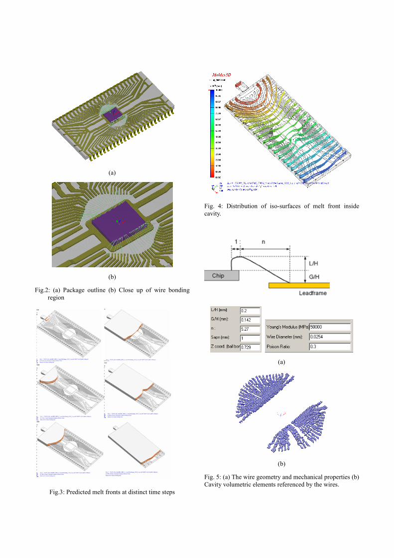
A TSOPII package with 53 wires is studied in this paper. The package size is 18.41x 10.16 x 1.0 mm3. The transfer time used for molding process is 11 seconds with mold temperature of 172oC. The molding compound is SUMITOMO 6300HJ. The outline of this package and the close-up view around the wire bonding region is shown in Fig. 2.

Fig. 3 illustrates the details of melt front advancement at distinct time steps. The melt front results indicate that the proposed methodology can predict the melt flow in the planar direction as well as the cross flow in the lateral direction. Fig. 4 further demonstrates the filling patterns by plotting the iso-surfaces of melt front inside cavity. The velocities and viscosity of resin flow from the 3D filling analysis can then be substituted into the Lamb’s model to evaluate the drag force for each wire. Then, the wire sweep deformation can be calculated by using the ABQUAS. The wire geometry and mechanical properties are displayed in Fig. 5(a). The wire bond profiles are defined by the parameters of wire span, wire height, die height and horizontal distance of the peak point from the wedge bond. All the wires used in the simulation have the same geometry values. The volume elements referenced by each wire are shown in Fig 5(b). It is these elements to be outputted to ABQUAS for wire deformation calculation. Fig 6(a) shows the predicted wire sweep index for each wire. The wires around the center have the largest deformation. This is because, these wires are the longest and also they are aligned almost perpendicular to the resin flow. The distribution of wire sweep index on each wire can be shown by the nodal wire sweep index as shown in Fig 6(b). Fig. 6(c) displays the three-dimensional wire deformation before and after resin flow.

Fig 7(a) compares the largest deformation of each wire obtained from prediction and experiment for the TSOP II package studied in this paper. The prediction from the present 3D approach shows reasonable agreements with the

experiment. Fig 7(b) shows the same comparison for another package PBGA 90L with 160 wires, which is not detailed in this paper. Again, the agreement between prediction and experiment is also reasonable.

Conclusions

A fully three-dimensional mathematical model and numerical technique has been developed to predict the encapsulate filling and the wire sweep. The proposed approach proved from the cases studied in this paper to be a reliable CAE tool for analyzing and further optimizing the IC encapsulation process.

Acknowledgement

The authors would like to thank the support from CoreTech Co. and NTHU through the Molding Technology Fundamental Research Project (Project No.0002182).

Reference

[1]. T. Nguyen, ASME Winter Ann. Meeting, 27-38 (1992)

[2]. S. Han and K.K. Wang, Trans. ASME, 117, 178-184 (1995)

[3]. M.R. Kamal and M.R. Ryan, Injection and Compression Molding Fundamentals, chap. 4, A.I.Isayev (Ed.), Marcel Dekker (1987).

[4]. R.Y. Chang, W.H. Yang, E. Chen, C. Lin and C.H. Hsu, SPE ANTEC Tech. Paper 1178-1181 (1998).

[5]. R.Y.Chang and W.H.Yang, Int. J. Numer. Methods Fluids, 37, 125-148 (2001).

Key Words: Three-Dimensional, CAE, IC Packaging, Mold

Filling, Wire Sweep.

Fig.1: 2D leadframe layout and the resulting 3D model.

(a)

(b)

Fig.2: (a) Package outline (b) Close up of wire bonding region

Fig.3: Predicted melt fronts at distinct time steps

Fig. 4: Distribution of iso-surfaces of melt front inside cavity.

(a)

(b)

Fig. 5: (a) The wire geometry and mechanical properties (b) Cavity volumetric elements referenced by the wires.

(a)

(b)

(c)

Fig. 6: (a) Wire sweep index (b) Nodal Wire sweep index (c) 3D view of wire deformation

TSOP 40L (53 wires)

0

0.5

1

1.5

2

2.5

3

3.5

1 6 11 16 21 26 31 36 41 46 51

Number of Wires

Wir

e Sw

eep

Inde

x (%

) Experiment

This work

(a)

PBGA 90L (160 wires)

0

0.5

1

1.5

2

2.5

3

3.5

4

4.5

5

1 11 21 31 41 51 61 71 81 91 101 111 121 131 141 151

Number of Wires

Wir

e S

wee

p In

dex

(%)

Experimental Data

This work

(b)

Fig.7: Wire sweep comparison of prediction and experiment (a) TSOP II (b) PBGA 90L.