Three dimensional elliptic solvers for interface problems and

applications

Shaozhong Deng∗ Kazufumi Ito† Zhilin Li‡

Abstract

Second order accurate elliptic solvers using Cartesian grids are presented for three dimen-sional interface problems in which the coefficients, the source term, the solution and its normalflux may be discontinuous across an interface. One of our methods is designed for general in-terface problems with variable but discontinuous coefficient. The scheme preserves the discretemaximum principle using constrained optimization techniques. An algebraic multigrid solver isapplied to solve the discrete system. The second method is designed for interface problems withpiecewise constant coefficient. The method is based on the fast immersed interface method anda fast 3D Poisson solver. The second method has been modified to solve Helmholtz/Poissonequations on irregular domains. An application of our method to an inverse interface problemof shape identification is also presented. In this application, the level set method is applied tofind the unknown surface iteratively.

Key words. 3D elliptic interface problem, irregular domain, discontinuous coefficient, discretemaximum preserving scheme, quadratic optimization, algebraic multigrid, shape identification, levelset method

AMS subject classifications. 65N06, 65N50

1 Introduction

In this paper, we develop two finite difference methods for three dimensional interface problemsusing Cartesian grids. Let Ω be a domain in R3 and Γ be an arbitrary piecewise smooth surface inΩ. The interface Γ divides Ω into two sub-domains Ω+ and Ω− and therefore Ω = Ω+ ∪ Ω− ∪ Γ.We consider the elliptic equation of the form

∇ · (β∇u(x, y, z)) + λ u(x, y, z) = f(x, y, z), (x, y, z) ∈ Ω− Γ, (1.1)

with a boundary condition on ∂Ω. The coefficients β, λ, and the source term f may be discontinuousacross the interface Γ.

∗Department of Mathematics, University of North Carolina at Charlotte, Charlotte, NC 28223, e-mail: shao-deng@uncc.edu

†Center for Research in Scientific Computation & Department of Mathematics, North Carolina State University,Raleigh, NC 27695, e-mail: kito@math.ncsu.edu

‡Center for Research in Scientific Computation & Department of Mathematics, North Carolina State University,Raleigh, NC 27695, e-mail: zhilin@math.ncsu.edu

1

Due to the discontinuity in the coefficient β, or/and the source/dipole distributions along theinterface Γ, the solution and the normal flux may be discontinuous across the interface Γ and canbe written as

[u] = w(s1, s2), [βun] = v(s1, s2), (1.2)

where w and v are two known functions defined only on the interface Γ, un = ∂u∂n = ∇u · n is the

limiting normal derivative of u, n is the unit normal vector pointing to Ω+ side. The interfaceΓ is expressed as a parametric form (x(s1, s2), y(s1, s2), z(s1, s2)), the jump [u ] is defined as thedifference of the limiting values of u from Ω+ and Ω− sides. We refer the readers to [7, 8, 9] formore discussions on the jump conditions.

The problem can be solved by body fitted finite element methods, see [2], for one example; theghost fluid method (GFM) [12] (which is first order accurate in the infinity norm but has a sym-metric linear system); fast solvers based on integral equations (assuming β is a piecewise constant),see [4, 13], for example; the immersed interface method (IIM) reported in [7, 17] for example; andpossibly some others. These methods have been described in details for two dimensional problems.Despite the fact that the extension of these methods to three dimensional (3D) problems may bestraightforward, the implementation of these methods in 3D can be very different and few haveappeared in the literature.

In this paper, we first develop the maximum principle preserving scheme for the interface prob-lems with variable but discontinuous coefficient by requiring the resulting finite difference matrixbe an M-matrix using constrained optimization techniques. The M-matrix condition guaranteesthe convergence of the algebraic multigrid solver [15] when it is applied to solve the linear systemof equations.

When the coefficient β is a piecewise constant, we propose a fast solver by transforming theoriginal problem (1.1) to a Poisson equation with an unknown jump in the normal derivative acrossthe interface Γ. We use a GMRES method to determine the unknown jump so that the originaljump in the flux is satisfied and thus the solution to the Poisson equation is also the solution to theoriginal problem (1.1). There are several advantages of this approach: (1) the computed solutionis second order accurate in the infinity norm; (2) the number of iterations in the GMRES methodis almost independent of the mesh sizes; (3) the computed normal derivatives are observed to besecond order accurate as well; (4) with slight changes, the methods can be, and have been appliedto Helmholtz/Poisson equations defined on irregular domains.

We also present an application of the second method to an electrical impedance tomographyproblem in identifying an unknown interface in a 3D domain. The inverse problem is solvediteratively by coupling the level set method [14] with the fast Poisson solver on irregular domainsdeveloped in this paper.

The paper is organized as the following. In Sec. 2, we introduce the interface relations ofthe problem which will be used in the derivation of our methods. The computational frame isestablished in Sec. 3. We propose the maximum principle preserving scheme for general coefficientin Sec. 4 and provide some numerical examples. The fast Poisson solver for piecewise constantcoefficient is proposed in Sec. 5 with some numerical examples. In Sec. 6, we present an applicationto an inverse problem of shape identification. We conclude the paper in Sec. 7.

2

2 Theoretical aspects

We hope to develop accurate finite difference methods based on Cartesian grids. To this end, wepresent a complete set of interface relations up to the second order derivatives by differentiatingthe jumps along the interface Γ, and making use of the original partial differential equation (PDE)(1.1). Since the flux jump condition [βun] is given in the normal direction of the interface, it isconvenient to use a local coordinates in the normal and tangential directions.

2.1 A local coordinate system

Given a point (x∗, y∗, z∗) on the interface Γ, let ξ be the normal direction of Γ, η and τ be twoorthogonal directions tangential to Γ, then the local coordinate transformation is given by

ξ = (x− x∗) αxξ + (y − y∗) αyξ + (z − z∗) αzξ

η = (x− x∗) αxη + (y − y∗) αyη + (z − z∗) αzη

τ = (x− x∗) αxτ + (y − y∗) αyτ + (z − z∗) αzτ ,

(2.3)

where αxξ represents the directional cosine between x-axis and ξ, and so forth, see Figure 1 for anillustration.

Figure 1: A sketch of a three dimensional local coordinate transformation.

The three dimensional coordinate transformation above can also be written in a matrix-vectorform. Define the local transformation matrix as

A =

αxξ αyξ αzξ

αxη αyη αzη

αxτ αyτ αzτ

, (2.4)

then we have ξ

ητ

= A

x− x∗

y − y∗

z − z∗

. (2.5)

3

Also, for any differentiable function p(x, y, z), we have pξ

pη

pτ

= A

px

py

pz

, (2.6)

where p(ξ, η, τ) = p(x, y, z), and pξξ pξη pξτ

pηξ pηη pητ

pτξ pτη pττ

= A

pxx pxy pxz

pyx pyy pyz

pzx pzy pzz

AT , (2.7)

where AT is the transpose of A. It is easy to verify that AT A = I, where I is the identity matrix.For two dimensional problems, the matrix-vector relations under the local coordinates can be foundin [3].

Note that under the local coordinate transformation (2.3), the PDE (1.1) is invariant, that is

(β ux)x + (β uy)y + (β uz)z + λu

= β (uxx + uyy + uzz) + βx ux + βy uy + βz uz + λu

= β (uξ ξ + uη η + uτ τ ) + (βx, βy, βz)

ux

uy

uz

+ λu

= β (uξ ξ + uη η + uτ τ ) + (βξ, βη, βτ )A−T AT

uξ

uη

uτ

+ λu

= β (uξ ξ + uη η + uτ τ ) + βξuξ + βηuη + βτ uτ + λu

= (βuξ)ξ + (βuη)η + (βuτ )τ + λu.

Therefore we will drop the bars for simplicity.

2.2 Interface relations

We use the superscripts + or − to denote the limiting values of a function from Ω+ side and Ω−

side of the interface respectively. Under the local coordinates, the limiting differential equationfrom the − side, for example, can be written as

β−(u−ξξ + u−ηη + u−ττ ) + β−ξ u−ξ + β−η u−η + β−τ u−τ + λ−u− − f− = 0. (2.8)

Also under the local ξ-η-τ coordinate system, the interface can be expressed as

ξ = χ(η, τ), with χ(0, 0) = 0, χη(0, 0) = 0, χτ (0, 0) = 0. (2.9)

We will use the jump condition (1.2) and the original differential equation to get more interfacerelations in this sub-section.

4

Let us first differentiate the first jump condition [u] = w in (1.2) with respect to η and τrespectively to get

[uξ]χη + [uη] = wη, (2.10)[uξ]χτ + [uτ ] = wτ . (2.11)

Differentiating (2.10) with respect to τ yields

χη∂

∂τ[uξ] + χητ [uξ] + [uηξ] χτ + [uητ ] = wητ . (2.12)

Differentiating (2.10) with respect to η and differentiating (2.11) with respect to τ respectively weobtain

χη∂

∂η[uξ] + χηη [uξ] + χη [uηξ] + [uηη] = wηη, (2.13)

χτ∂

∂τ[uξ] + χττ [uξ] + χτ [uτξ] + [uττ ] = wττ . (2.14)

Before differentiating the jump of the normal derivative [βun] = v in (1.2), we first express theunit normal vector of the interface Γ as

n =(1, −χη, −χτ )√

1 + χη2 + χτ

2. (2.15)

So the second interface condition [βun] = v in (1.2) can be written as

[ β ( uξ − uη χη − uτ χτ ) ] = v(η, τ)√

1 + χη2 + χτ

2. (2.16)

Differentiating this with respect to η gives

[ (βξ χη + βη ) (uξ − uη χη − uτ χτ ) ]

+[

β

(uξξ χη + uξη − χη

∂

∂ηuη − χτ

∂

∂ηuτ − uη χηη − uτ χητ

)]

= vη

√1 + χη

2 + χτ2 + v

χη χηη√1 + χη

2 + χτ2.

(2.17)

Similarly, differentiating (2.16) with respect to τ gives

[ ( βξ χτ + βτ ) (uξ − uη χη − uτ χτ ) ]

+[

β

(uξξ χτ + uξτ − χη

∂

∂τuη − χτ

∂

∂τuτ − uη χητ − uτ χττ

)]

= vτ

√1 + χη

2 + χτ2 + v

χτ χττ√1 + χη

2 + χτ2.

(2.18)

5

At the origin, χη(0, 0) = χτ (0, 0) = 0, and from (2.10)–(2.18) we can conclude that

u+ = u− + w,

u+ξ =

β−

β+u−ξ +

v

β+,

u+η = u−η + wη,

u+τ = u−τ + wτ ,

u+ητ = u−ητ + (u−ξ − u+

ξ )χητ + wητ ,

u+ηη = u−ηη + (u−ξ − u+

ξ )χηη + wηη,

u+ττ = u−ττ + (u−ξ − u+

ξ )χττ + wττ ,

u+ξη =

β−

β+u−ξη +

(u+

η −β−

β+u−η

)χηη +

(u+

τ −β−

β+u−τ

)χητ

+β−ηβ+

u−ξ −β+

η

β+u+

ξ +vη

β+,

u+ξτ =

β−

β+u−ξτ +

(u+

η −β−

β+u−η

)χητ +

(u+

τ −β−

β+u−τ

)χττ

+β−τβ+

u−ξ −β+

τ

β+u+

ξ +vτ

β+.

(2.19)

To get the relation for u+ξ ξ we need to use the differential equation (1.1) itself from which we can

write[ β (uξξ + uηη + uττ ) + βξuξ + βηuη + βτuτ + λu ] = [f ] . (2.20)

Notice that

λ−u− − λ+u+ = λ−u− − λ+u− + λ+u− − λ+u+ = −[λ]u− − λ+[u]. (2.21)

Rearranging equation (2.20) and using (2.21) above we get

β+(u+

ξ ξ + u+η η + u+

ττ

)+ β+

ξ u+ξ + β+

η u+η + β+

τ u+τ =

β−(u−ξ ξ + u−η η + u−ττ

)+ β−ξ u−ξ

+ β−η u−η + β−τ u−τ + [f ] + λ−u− − λ+u+.

(2.22)

Plugging the sixth and seventh equations of (2.19) in (2.22) and collecting terms finally we have

u+ξ ξ =

β−

β+u−ξ ξ +

(β−

β+− 1

)u−η η +

(β−

β+− 1

)u−ττ+

u+ξ

(χηη + χττ −

β+ξ

β+

)− u−ξ

(χηη + χττ −

β−ξβ+

)

+1

β+

(β−η u−η − β+

η u+η

)+

1β+

(β−τ u−τ − β+

τ u+τ

)− 1

β+

([λ]u− + λ+[u]

)+

[f ]β+

− wηη − wττ .

(2.23)

6

3 The computational frame

For simplicity, we assume that the domain Ω is a solid cube, say [a1, b1]× [a2, b2]× [a3, b3]. We wishto solve the problem using a finite difference method and a uniform Cartesian grid with

xi = a1 + ih, yj = a2 + jh, zk = a3 + kh, 0 ≤ i ≤ L, 0 ≤ j ≤ M, 0 ≤ k ≤ N.

We also assume that h = (b1 − a1)/L = (b2 − a2)/M = (b3 − a3)/N to make many expressionssimple.

We use the zero level surface of a three dimensional function ϕ(x, y, z) to express the interface,that is

ϕ(x, y, z) < 0, if (x, y, z) ∈ Ω−,

ϕ(x, y, z) = 0, if (x, y, z) ∈ Γ,

ϕ(x, y, z) > 0, if (x, y, z) ∈ Ω+.

(3.24)

We assume that the level set function is Lipschitz continuous and ϕ(x, y, z) ∈ C2 in the smallneighborhood of the zero level set ϕ = 0 that represents the interface Γ. At a grid point xijk,let ϕmin

ijk and ϕmaxijk be the minimum and maximum values of the level set function ϕ at ϕi±1,j,k,

ϕi,j±1,k, ϕi,j,k±1, and ϕijk. We define xijk as an irregular grid point if

ϕmaxijk ϕmin

ijk ≤ 0. (3.25)

Otherwise xijk is called a regular grid point.

3.1 Setting-up a local coordinate system using the level set function

Given a point X∗ = (x∗, y∗, z∗) on the interface, we choose the ξ direction as the normal directionof the interface

ξ =∇ϕ

|∇ϕ| = (ϕx, ϕy, ϕz)T /√

ϕ2x + ϕ2

y + ϕ2z,

where the unit normal direction is evaluated at (x∗, y∗, z∗). The η- and τ - axes are in the tangentplane passing through (x∗, y∗, z∗). We choose the first tangential direction as

η = (ϕy, −ϕx, 0)T /√

ϕ2x + ϕ2

y ,

if ϕ2x + ϕ2

y 6= 0. Otherwise we choose

η = (ϕz, 0, −ϕx)T /√

ϕ2x + ϕ2

z .

The corresponding second tangential direction is

τ =s|s| , where s = (ϕxϕz, ϕyϕz, −ϕ2

x − ϕ2y)

T ,

if ϕ2x + ϕ2

y 6= 0. Otherwise we choose

τ =t|t| , where t = (−ϕxϕy, ϕ2

x + ϕ2z, −ϕyϕz)T .

7

3.2 Computing the projections

For each irregular grid point x = (xi, yj , zk), we select a point X∗ = (x∗i , y∗j , z

∗k) on the interface.

Although not necessarily, we take this point as the projection of (xi, yj , zk) on the interface. Theprojection X∗ is the closest point on the interface to the grid point (xi, yj , zk) with ϕ(X∗) = 0. Inpractice, we can only compute the projection approximately. Since the interface Γ is representedas the zero level surface ϕ = 0, and the level set function ϕ has the fastest rate of increase/decreasein the normal direction of the level surfaces, we write the projection as

X∗ = x + αp,

where p = ∇ϕ/|∇ϕ|, and α ∼ h is an approximation of the signed distance from the grid point x tothe projection X∗. Neglecting O(α3) and higher order terms in the Taylor expansion of ϕ(X∗) = 0,we get a quadratic equation for α

ϕ(x) + |∇ϕ|α +12

(pT He(ϕ)p)α2 = 0,

where He(ϕ) is the Hessian matrix of ϕ

He(ϕ) =

ϕxx ϕxy ϕxz

ϕyx ϕyy ϕyz

ϕzx ϕzy ϕzz

.

The values of ϕ, ϕx, ϕy, ϕz, ϕxx, ϕxy, ϕxz, ϕyy, ϕyz, and ϕzz are all computed at the grid pointx = (xi, yj , zk) using the standard central finite difference scheme. Since the truncation error of theabove quadratic expansion is of O(α3) ∼ O(h3), and the central finite difference schemes are secondorder accurate, and the quantities ϕx, ϕy, and ϕz appear in the linear and quadratic terms of α,and the second order derivatives ϕxx, · · · , ϕzz appear in the quadratic term of α, the computedprojections are third order accurate.

4 The maximum principle preserving scheme

We now derive a finite difference equation of the formns∑m

γm ui+im,j+jm,k+km + λijk uijk = fijk + Cijk, (4.26)

at every grid point (xi, yj , zk) to approximate (1.1), where im, jm, km take values from 0,±1,±2 · · · ,meaning that the summation is taken over the neighboring grid points centered at (xi, yj , zk). Notethat we have omitted the dependency of m on i, j, and k, for simplicity. At a regular grid point,we use the standard seven point finite difference scheme

γi−1,jk =βi−1/2,j,k

h2, γi+1,jk =

βi+1/2,j,k

h2, γi,j−1,k =

βi,j−1/2,k

h2,

γi,j+1,k =βi,j+1/2,k

h2, γi,j,k−1 =

βi,j,k−1/2

h2, γi,j,k+1 =

βi,j,k+1/2

h2,

γi,j,k = − (γi−1,jk + γi+1,jk + γi,j−1,k + γi,j+1,k + γi,j,k−1 + γi,j,k+1) , Cijk = 0

(4.27)

where βi−1/2,j,k = β(xi − h/2, yj , zk) and so forth. The local truncation errors are O(h2).

8

4.1 Setting-up the finite difference equations at irregular grid points

At irregular grid points, we use the method of un-determined coefficients to find the coefficientsof the finite difference scheme. Let X∗ be the projection of (xi, yj , zk) on the interface. Using theTaylor expansion from both sides of the interface at X∗, we can write

ns∑m

γm u(xi+im , yj+jm , zk+km) + λijk u(xi, yj , zk)

=ns∑m

γm

(u± + u±ξ ξm + u±η ηm + u±τ τm +

ξ2m

2u±ξξ +

η2m

2u±ηη

+τ2m

2u±ττ + ξmηm u±ξη + ξmτm u±ξτ + ηmτm u±ητ + O(h3)

)+ λijk (uijk + O(h)),

(4.28)

where the function values and the derivatives are defined as the limiting value at X∗ from the sidewhere the grid point (i + im, j + jm, k + km) is in. Using the interface relations (2.19) and (2.23),the expression above can be written as

ns∑m

γm u(xi+im , yj+jm , zk+km) + λijk u(xi, yj , zk) ≈a1 u− + a2 u+ + a3 u−ξ + a4 u+

ξ + a5 u−η + a6 u+η + a7 u−τ + a8 u+

τ

+ a9 u−ξ ξ + a10 u+ξ ξ + a11 u−η η + a12 u+

η η + a13 u−ττ

+ a14 u+ττ + a15 u−ξ η + a16 u+

ξ η + a17 u−ξτ + a18 u+ξτ

+ a19 u−ητ + a20 u+ητ + λ− u−,

(4.29)

with the higher order terms being neglected, where the coefficients ai’s depend only on the positionof the stencil relative to the interface. They are independent of the functions u, β, λ, and f . If wedefine the index sets K+ and K− by

K± = m : (ξm, ηm, τm) is on the ± side of Γ , (4.30)

then the ai’s with odd subscript are given by

a1 =∑

m∈K−γm, a3 =

∑m∈K−

γm ξm, a5 =∑

m∈K−γm ηm, a7 =

∑m∈K−

γm τm,

a9 =12

∑m∈K−

γm ξ2m, a11 =

12

∑m∈K−

γm η2m, a13 =

12

∑m∈K−

γm τ2m, (4.31)

a15 =∑

m∈K−γm ξmηm, a17 =

∑m∈K−

γm ξmτm, a19 =∑

m∈K−γm ηmτm.

The ai’s with even subscript are exactly the same as above except the summation is from the subsetK+. Substituting the interface relations (2.19) and (2.23), we express all the quantities from the+ side in terms of the quantities from the − side. Thus the right hand side of (4.29) is representedby the linear combination of the quantities from the − side. After some manipulations, (4.29) is

9

arranged as follows

ns∑m

γm u(xi+im , yj+jm , zk+km) + λijk u(xi, yj , zk)

= ( )u− + ( )u−ξ + ( )u−η + ( )u−τ + ( )u−ξξ + ( )u−ηη

+ ( )u−ττ + ( )u−ξη + ( )u−ξτ + ( )u−ητ + Cijk.

(4.32)

The contents in the parenthesis are the corresponding terms in the left hand side of (4.33)-(4.42).The last term Cijk is a linear function of the jumps in the solution and the flux and is given in(4.43). We want the finite difference scheme to be second order accurate to the differential equation.Therefore at X∗ we match (4.29) with the PDE (2.8) from the − side, i.e., we equate (4.32) toβ− (u−ξξ + u−ηη + u−ττ ) + β−ξ u−ξ + β−η u−η + β−τ u−τ . Hence we obtain the linear system of equations forthe coefficients γi’s below:

a1 − a10[λ]β+

+ a2 = 0, (4.33)

a3 − a10

(χηη + χττ −

β−ξβ+

)+ a12 χηη + a14 χττ + a16

β−ηβ+

+ a18β−τβ+

+ a20 χητ +β−

β+

a4 + a10

(χηη + χττ −

β+ξ

β+

)

−a12 χηη − a14 χττ − a16

β+η

β+− a18

β+τ

β+− a20 χητ

= β−ξ , (4.34)

a5 + a10

β−ηβ+

− a16β−

β+χηη − a18

β−

β+χητ

+ a6 − a10

β+η

β++ a16 χηη + a18 χητ = β−η , (4.35)

a7 + a10β−τβ+

− a16β−

β+χητ − a18

β−

β+χττ

+ a8 − a10β+

τ

β++ a16 χητ + a18 χττ = β−τ , (4.36)

a9 + a10β−

β+= β−, (4.37)

a11 + a12 + a10

(β−

β+− 1

)= β−, (4.38)

a13 + a14 + a10

(β−

β+− 1

)= β−, (4.39)

a15 + a16β−

β+= 0, (4.40)

a17 + a18β−

β+= 0, (4.41)

a19 + a20 = 0. (4.42)

10

If we can solve this linear system of equations to get γi’s, then by collecting the remaining termsin (4.29), we can determine the correction term which is given by

Cijk = a10

([f ]β+

− λ+ w

β+− wηη − wττ

)+ a12 wηη + a14 wττ

+ a16vη

β++ a18

vτ

β++ a20 wητ + a2 w

+1

β+

a4 + a10

(χηη + χττ −

β+ξ

β+

)− a12 χηη

− a14 χττ − a16

β+η

β+− a18

β+τ

β+− a20 χητ

v

+

(a6 − a10

β+η

β++ a16 χηη + a18 χητ

)wη

+(

a8 − a10β+

τ

β++ a16 χητ + a18 χττ

)wτ .

(4.43)

4.2 Computing the principal curvatures using the level set function

In order to determine the matrix entries of the linear system of equations (4.33)–(4.42) for thecoefficients γi’s, we need to compute the second order tangential derivatives χηη, χττ , χτη of χ atX∗. We call these quantities principal curvatures. These quantities are computed from the levelset function. Since ϕ(χ(η, τ), η, τ) = 0, it follows from the implicit function theory that

ϕη + ϕξχη = 0, (4.44)

ϕτ + ϕξχτ = 0. (4.45)

and

ϕηη + ϕηξχη + (ϕξη + ϕξξχη)χη + ϕξχηη = 0,

ϕητ + ϕηξχτ + (ϕξτ + ϕξξχτ )χη + ϕξχητ = 0,

ϕττ + ϕτξχτ + (ϕξτ + ϕξξχτ )χτ + ϕξχττ = 0.

So, we have

χηη = −ϕηη/ϕξ

χττ = −ϕττ/ϕξ

χητ = −ϕητ/ϕξ,(4.46)

where (ϕξ, ϕη, ϕτ ) and (ϕξξ, ϕηη, ϕττ ) are given in (2.6) and (2.7), respectively. Our procedure forevaluating the principal curvatures includes:

• Compute the first and second derivatives of ϕ at the surrounding grid points using the stan-dard central difference scheme.

11

• Use the bi-linear interpolation to compute the first and second order derivatives ϕx, ϕy, · · · ,ϕzz in the original coordinates at the projection point X∗.

• Use the formula (2.6)–(2.7) to get the first order derivatives ϕξ, ϕη, and ϕτ .

• Use the formula (4.46) to compute the principal curvatures ϕη,η, ϕη,τ , and ϕτ,τ in the localcoordinates.

The bi-linear interpolation uses eight grid points. Given any point (x∗, y∗, z∗) on the interface,we can find a cube containing the point with the eight vertices (x0, y0, z0), (x0, y0, z1), (x0, y1, z0),(x0, y1, z1), (x1, y0, z0), (x1, y0, z1), (x1, y1, z0), and (x1, y1, z1). Let Qijk be the function values atthe eight vertices. The eight point bi-linear interpolation is defined as

Q(x∗, y∗, z∗) =18

1∑i,j,k=0

Qijk xi yj zk, (4.47)

where

xi = 1 + (2i− 1)(

2(x− x0)h

− 1)

, yj = 1 + (2j − 1)(

2(y − y0)h

− 1)

,

zk = 1 + (2k − 1)(

2(z − z0)h

− 1)

.

(4.48)

4.3 Computing the tangential derivatives of interface quantities

In the evaluation of the correction terms Cijk, we need to compute the tangential derivatives suchas wη, wτ , wηη, wττ , wητ , vη, and vτ , where w and v are only defined along the interface Γ. Theyare computed using the least squares interpolation.

Let g be a function defined on the interface and therefore we know its values at the projectionsX∗

p. We explain below how to compute its tangential derivatives at a particular projection X∗ usingthe projections X∗

p in the neighborhood of X∗.

In the neighborhood of X∗, the interface quantity g can be written as g(η, τ) using the localcoordinates. The least squares interpolation for gη, gτ , and gηη at X∗, for example, can be writtenas

gη(X∗) =∑

|X∗−X∗p|≤Rε

αp gp, gτ (X∗) =∑

|X∗−X∗p|≤Rε

λp gp,

gηη(X∗) =∑

|X∗−X∗p|≤Rε

σp gp,

(4.49)

where gp = g(X∗p) are the function values at the projections X∗

p, Rε is a pre-chosen parameterbetween 5.1h ∼ 6.1h. We should choose Rε such that at least ten points are involved. We explainhow to compute the coefficients αp for gη(X∗) as an illustration. It is based on the Taylor expansionand the singular value decomposition (SVD) to solve an under-determined system of equations.

12

Using the Taylor expansion at X∗, we have∑|X∗p−X∗|≤Rε

αp gp =∑

|X∗p−X∗|≤Rε

αp

(g∗ +∇g∗ · (X∗

p −X∗) +12(X∗

p −X∗)T H(g∗)(X∗p −X∗) + · · ·

)

= ( )g∗ + ( )g∗η + ( )g∗τ + ( )g∗ηη + ( )g∗ητ + ( )g∗ττ + h.o.t,

where H(g∗) is the Hessian matrix of g∗ in terms of the variables η and τ under the local coordinatesξ-η-τ centered at the projection X∗, h.o.t stands for the high order terms of |X∗

p −X∗|, and thecontents in the parentheses are the corresponding right hand side in the system of equations below.Using the method of the under-determined coefficient, we set∑

p

αp = 0,∑

p

αpηp = 1,∑

p

αpτp = 0,

∑p

αpη2p = 0,

∑p

αpτ2p = 0,

∑p

αpηpτp = 0,(4.50)

where (ηp, τp)’s are the coordinates of the projections X∗p on the interface in the parametric form

ξ = χ(η, τ) centered at X∗. The under-determined system is solved by the SVD subroutine formLAPACK/LINPACK which is available from the Netlib. The other tangential derivatives can becomputed in the same way with different right hand side. Since the coefficients matrix is the same,we just need to compute the SVD once.

4.4 An optimization approach

After the preparations from previous sub-sections, we are ready to determine the coefficients γm’sand ns in the finite difference equation in (4.26) for all irregular grid points. It seems that wecan take ns = 10 because there are ten equations (4.33)–(4.42). The problem is that we can notguarantee that the system (4.33)–(4.42) have a solution and the stability of the resulting system ofthe finite difference equations.

We propose the maximum principle preserving scheme by choosing ns > 10 and adding the signconstraints

γm < 0, if (im, jm, km) = (0, 0, 0),

γm ≥ 0, if (im, jm, km) 6= (0, 0, 0),(4.51)

in addition to the linear system of equations (4.33)–(4.42). The sign constraints will guarantee thecoefficient matrix of the system of the finite difference equations be an M-matrix.

To solve the linear system of equations (4.33)–(4.42) with the inequality constraints (4.51), weconstruct a quadratic optimization problem

minγ

12

∑m

(γm − dm)2, (4.52)

s.t.Bγ = b, the system of (4.33)–(4.42),

γm < 0, if (im, jm, km) = (0, 0, 0),

γm ≥ 0, if (im, jm, km) 6= (0, 0, 0),(4.53)

13

where γ = (γ1, γ2, · · · , γns)T is the vector composed of the coefficients of the finite differencescheme, and Bγ = b denotes the equality constraints specified by (4.33)–(4.42). We also want tochoose γm’s in such a way that the finite difference scheme (4.26) reduces to the standard centralfinite difference scheme if there is no interface or the coefficient β of the PDE is continuous acrossthe interface. This can be done by choosing

dm =βi+im/2,j+jm/2,k+km/2

h2, if (im, jm, km) is one of the six neighbors of (0, 0, 0),

d0 = − 1h2

∑m,m6=0

βi+im/2, j+jm/2, k+km/2, (4.54)

dm = 0, otherwise,

where the summation is over the six neighbors of the grid point (xi, yj , zk) and βi−1/2,j,k = β(xi −h/2, yj , zk) and so forth.

There are several commercial and educational software packages that are designed to solve con-strained quadratic optimization problems, such as QP in Matlab and QL by K. Schittkowski [16].

What the minimum ns should be that can guarantee the existence of the solution to the op-timization problem is still an open theoretical problem. In our implementation, we take all thegrid points in the cube centered at (xi, yj , zk), that is ns = 27. We have not experienced anynumerical failure for our testing problems. In [11], the authors numerically showed the existence ofthe solution to the optimization problem in two space dimensions. We believe that the conclusionsare also true in three dimensions.

If the optimization problem has a solution at all irregular grid points, then it is shown in [11]that the solution to the finite difference scheme has second order accuracy globally in the infinitynorm. We omit the proof here since it is essentially the same as in two space dimensions.

We summarize our algorithm for the elliptic interface problem with variable but discontinuouscoefficient below.

• Set-up a Cartesian grid.

• Label the grid points as regular, irregular.

• Find the projections of irregular grid points on the interface as described in Sec. 3.2.

• At each irregular grid point, calculate the local coordinates (ξm, ηm, τm) for 27 neighboringgrid points. Calculate the matrix B and vectors b from the system (4.33)-(4.42), and di

from (4.54). Solve the quadratic programming (4.52)–(4.53) for γm’s and then compute thecorrection term Cijk using (4.43).

• Use the formula (4.27) as the finite difference scheme at regular grid points.

• Form the system of the finite difference equations (4.26).

• Solve the system of the finite difference equations (4.26) to get an approximate solution tothe PDE.

14

4.5 An algebraic multigrid solver

If the coefficient β not only has a jump across the interface, but also is a function of location (x, y, z),there are almost no fast elliptic solvers that can be used to solve the linear system of equationsobtained from our maximum principle preserving scheme. The Gauss-Seidel or SOR method is tooslow in convergence. We use the algebraic multigrid method (AMG) developed by the GermanNational Research Center for Information Technology (GMD) which is available on the Internet,see also [15]. The AMG has been shown to be a robust and efficient solver for a linear system ofequations Qu = F with certain properties. The AMG is guaranteed to converge if the coefficientmatrix Q satisfies one of the following conditions:

• Q is positive/negative definite or semi-positive/negative definite with ROWSUM =0 for eachrow, where ROWSUM denotes the sum of the entries in each row.

• Q is “essentially” positive type, i.e.,

– The diagonal entries of Q must be positive/negative.

– Most of the off-diagonal entries of Q are non-positive/non-negative.

– For each row, the ROWSUM should be non-negative/non-positive.

The linear system of equations derived from the maximum principle preserving scheme is “essen-tially” negative definite matrix (an M-matrix) and the algebraic multigrid solver can be applied.Our numerical experiments showed that the AMG method generally converged faster than the SORmethod. The speed-up increases as the size of the mesh gets larger.

4.6 Numerical results for the maximum principle preserving scheme

We have done a number of numerical experiments which confirm second order accuracy of the max-imum principle preserving scheme. The numerical tests are done using Sun Ultra 10 workstationsor the CRAY T916 supercomputer at the North Carolina Supercomputing Center (NCSC). Thecomputational domain is [−1, 1]× [−1, 1]× [−1, 1]. In all examples, L = M = N , and ns = 27 (i.e.,all 27 grid points involved in the usual 27 point stencil) unless otherwise specified. The convergencetolerance for the algebraic multigrid method is 10−5.

Example 4.1 We present an example with a variable and discontinuous coefficient β. The inter-face is a sphere x2 + y2 + z2 = 1/4. The differential equation is

(βux)x + (βuy)y + (βuz)z = f,

where

β(x, y, z) =

r2 + 1, if r < 1

2 ,

b, if r ≥ 12 ,

f(x, y, z) = 10 r2 + 6,

15

and b is a constant and r =√

x2 + y2 + z2. The Dirichlet boundary condition is determined fromthe exact solution

u(x, y, z) =

r2, if r < 12 ,(

r4

2+ r2

)/b−

(r40

2+ r2

0

)/b + r2

0, if r ≥ 12 ,

(4.55)

where r0 = 1/2.

It can be calculated that [u] = 0 and [βun] = 0 in this example. However, the normal derivativeun is discontinuous due to the discontinuity in the coefficient β.

The jump in the coefficient β depends on the choice of the constant b. We tested three differentcases, b = 1, b = 10 (small jump), and b = 1000 (large jump). Table 1 shows the results of the gridrefinement analysis. The maximum relative error is defined as

‖ EN ‖∞ =maxi,j,k

| u(xi, yj , zk)− uijk |maxi,j,k

| u(xi, yj , zk) | , (4.56)

where uijk is the computed approximation to the exact one u(xi, yj , zk). We also display the ratioof two successive errors

ratio =‖ EN ‖∞‖ E2N ‖∞

. (4.57)

In Table 1, we see that the average ratio approaches number 4 indicating second order accuracy ofthe maximum principle preserving scheme.

Table 1: The grid refinement analysis for Example 4.1.

b = 1 b = 10 b = 1000L×M ×N ‖ EN ‖∞ ratio ‖ EN ‖∞ ratio ‖ EN ‖∞ ratio26× 26× 26 1.247× 10−3 1.525× 10−3 3.485× 10−3

52× 52× 52 3.979× 10−4 3.134 5.240× 10−4 2.910 1.111× 10−3 3.137104× 104× 104 9.592× 10−5 4.148 1.010× 10−4 5.188 1.605× 10−4 6.922

Example 4.2 Now we present an example of multi-connected domain and discontinuous solution.The level set function is

ϕ(x, y, z) = S1(x, y, z)S2(x, y, z),

where

S1(x, y, z) = (x− 0.2)2 + 2(y − 0.2)2 + z2 − 0.01,

S2(x, y, z) = 3(x + 0.2)2 + (y + 0.2)2 + z2 − 0.01.

16

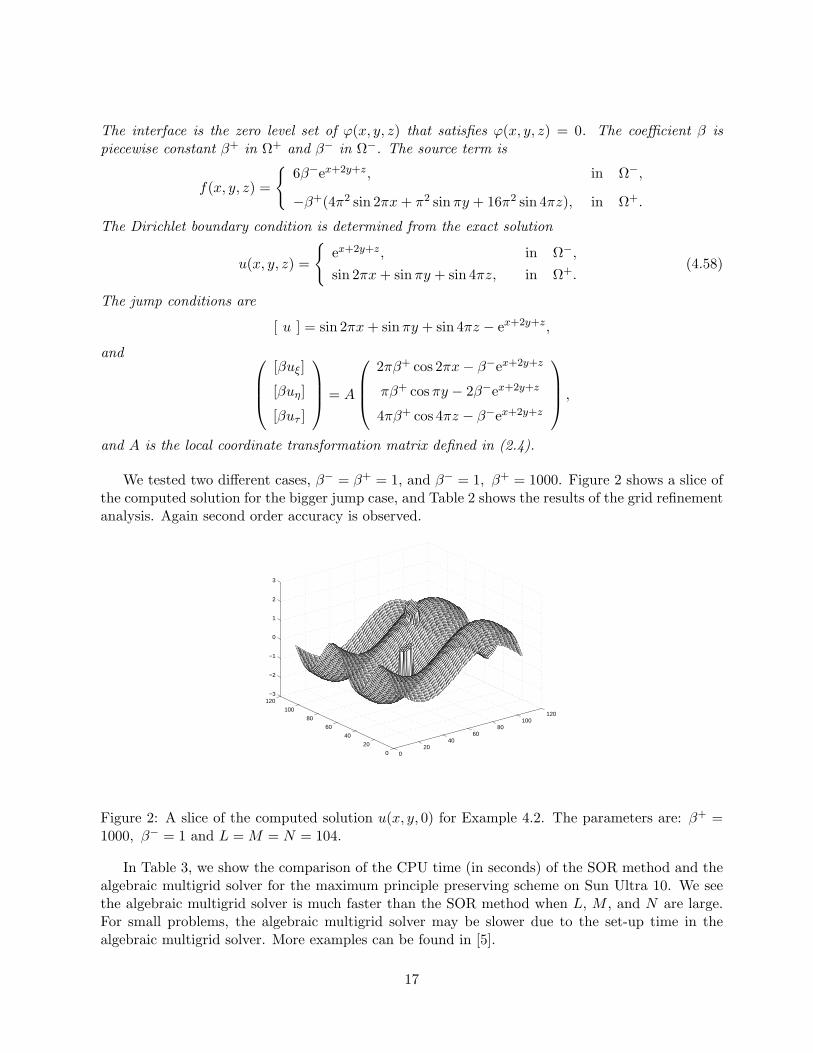
The interface is the zero level set of ϕ(x, y, z) that satisfies ϕ(x, y, z) = 0. The coefficient β ispiecewise constant β+ in Ω+ and β− in Ω−. The source term is

f(x, y, z) =

6β−ex+2y+z, in Ω−,

−β+(4π2 sin 2πx + π2 sin πy + 16π2 sin 4πz), in Ω+.

The Dirichlet boundary condition is determined from the exact solution

u(x, y, z) =

ex+2y+z, in Ω−,

sin 2πx + sinπy + sin 4πz, in Ω+.(4.58)

The jump conditions are

[ u ] = sin 2πx + sinπy + sin 4πz − ex+2y+z,

and

[βuξ]

[βuη]

[βuτ ]

= A

2πβ+ cos 2πx− β−ex+2y+z

πβ+ cos πy − 2β−ex+2y+z

4πβ+ cos 4πz − β−ex+2y+z

,

and A is the local coordinate transformation matrix defined in (2.4).

We tested two different cases, β− = β+ = 1, and β− = 1, β+ = 1000. Figure 2 shows a slice ofthe computed solution for the bigger jump case, and Table 2 shows the results of the grid refinementanalysis. Again second order accuracy is observed.

020

4060

80100

120

0

20

40

60

80

100

120−3

−2

−1

0

1

2

3

Figure 2: A slice of the computed solution u(x, y, 0) for Example 4.2. The parameters are: β+ =1000, β− = 1 and L = M = N = 104.

In Table 3, we show the comparison of the CPU time (in seconds) of the SOR method and thealgebraic multigrid solver for the maximum principle preserving scheme on Sun Ultra 10. We seethe algebraic multigrid solver is much faster than the SOR method when L, M , and N are large.For small problems, the algebraic multigrid solver may be slower due to the set-up time in thealgebraic multigrid solver. More examples can be found in [5].

17

Table 2: The grid refinement analysis for Example 4.2.

β+ = 1, β− = 1 β+ = 1000, β− = 1L×M ×N ‖ EN ‖∞ ratio ‖ EN ‖∞ ratio52× 52× 52 3.108× 10−2 2.032× 10−2

104× 104× 104 6.758× 10−3 4.599 4.771× 10−3 4.259

Table 3: Comparison of CPU time (in seconds) of the SOR method and the AMG method on SunUltra 10.

Example 4.1 Example 4.2L×M ×N (b = 107) (β+ = 104, β− = 1)

SOR AMG SOR AMG20× 20× 20 0.21 1.57 0.06 0.8340× 40× 40 27.51 25.56 29.62 13.8980× 80× 80 1410.54 265.26 1464.57 265.84

4.7 A special case

When β and λ are continuous but the solution and/or the normal derivative have jumps across theinterface, the maximum principle preserving method becomes the standard central finite differencescheme. Furthermore if β is a constant, we have the following theorem.

Theorem 4.1 If β(x, y, z) is a constant β and λ is continuous, then the solution of equations(4.33)–(4.42) are

γi−1,jk = γi+1,jk = γi,j−1,k = γi,j+1,k = γij,k−1 = γij,k+1 =β

h2, γijk = −6 β

h2, (4.59)

and all other coefficients γi+im,j+jm,k+km = 0. The solution above is also a solution to the con-stained optimization problem.

Proof: We only need to verify that these γijk’s satisfy the linear system of equations (4.33)–(4.42) at any irregular grid point. Without loss of generality, we assume the irregular grid point(xi, yj , zk) be the origin. The continuity condition of λ means [λ] = 0, and a constant β means[β] = 0. We also have ρ = β−/β+ = 1, βξ = βη = βτ = 0, etc. Therefore the linear system ofequations (4.33)–(4.42) becomes

a1 + a2 = 0, a3 + a4 = 0,a5 + a6 = 0, a7 + a8 = 0,

a9 + a10 = β, a11 + a12 = β,a13 + a14 = β, a15 + a16 = 0,a17 + a18 = 0, a19 + a20 = 0.

18

The first equation

a1 + a2 = 0, i.e.∑m

γm = 0,

is obviously true. Under the transformation (2.3), let the new coordinates corresponding to (0, 0, 0),(−h, 0, 0), (h, 0, 0), (0,−h, 0), (0, h, 0), (0, 0,−h) and (0, 0, h) be (ξm, ηm, τm), m = 1, . . . , 7. Define

Ym =

ξm

ηm

τm

, m = 1, 2, . . . , 7,

and

X1 =

−x∗

−y∗

−z∗

, X2 =

−h− x∗

−y∗

−z∗

, X3 =

h− x∗

−y∗

−z∗

, X4 =

−x∗

−h− y∗

−z∗

,

X5 =

−x∗

h− y∗

−z∗

, X6 =

−x∗

−y∗

−h− z∗

, X7 =

−x∗

−y∗

h− z∗

.

We can verifyYm = AXm, m = 1, 2, . . . , 7,

and a3 + a4

a5 + a6

a7 + a8

=

∑m

γmξm∑m

γmηm∑m

γmτm

=

∑m

γmYm =∑m

γmAXm

=β

h2A

6x∗ − h− x∗ + h− x∗ − x∗ − x∗ − x∗ − x∗

6y∗ − y∗ − y∗ − h− y∗ + h− y∗ − y∗ − y∗

6z∗ − z∗ − z∗ − z∗ − z∗ − h− z∗ + h− z∗

=

0

00

.

Therefore, the second to the fourth equations (4.34)–(4.36) are also satisfied. To prove the rest, wecan easily verify

∑m

γm Xm XTm =

2β 0 0

0 2β 0

0 0 2β

= 2βI.

Therefore we have ∑m

γm

2Ym YT

m =12

∑m

γm AXm XTmAT = βI,

19

since AAT = I, where A is defined in (2.4). Furthermore, we have the following

∑m

γm

2Ym YT

m =

∑m

γm

2ξ2m

∑m

γm

2ξmηm

∑m

γm

2ξmτm

∑m

γm

2ξmηm

∑m

γm

2η2

m

∑m

γm

2ηmτm

∑m

γm

2ξmτm

∑m

γm

2ηmτm

∑m

γm

2τ2m

,

which implies that

a9 + a10 = a11 + a12 = a13 + a14 = β,

a15 + a16 = a17 + a18 = a19 + a20 = 0.

This concludes the proof. 2

The result above tells us that for Poisson equations, the standard central finite difference schemecan be applied directly with the right hand side being modified by Cijk even if the solution and/orthe normal derivative have jumps. Fast Poisson solvers such as the one from the Fishpack [1] canbe used to solve the resulting linear system.

5 A fast Poisson solver for piecewise constant coefficient

In this section, we discuss a fast algorithm for solving the Poisson equation (1.1), (1.2) when β ispiecewise constant in the domain Ω and λ ≡ 0. Divided by the coefficient in each sub-domain ofΩ, the original problem can be written as

∆u =f

β+, if (x, y, z) ∈ Ω+,

∆u =f

β−, if (x, y, z) ∈ Ω−,

(5.60a)

[u] = w, [βun] = v, (5.60b)

Given BC on ∂Ω. (5.60c)

The Poisson equation is only valid in the interior of the domain excluding the interface Γ. ThePoisson equation can be solved readily with a fast 3D Poisson solver if we know the jump inthe solution [u] = w and the jump in the normal derivative [un]. This is because the system ofthe finite difference equations (4.26) for uijk reduces to the standard seven point discrete Poissonequation with modified right hand side, see Sec. 4.7. However, the second jump condition for theoriginal problem (1.1) is in the flux [βun] = v instead of [un]. We cannot divide β from the fluxjump condition because β is discontinuous. In [10], a fast method for two dimensional problems isproposed. In this section, we describe our algorithm for three dimensional problems.

As described in [10], the idea is to augment the unknown [un] = g and equation [βun] = v to(5.60a). That is, we determine an interface function g(s1, s2) in such a way that the solution u(g)to (5.60a) satisfies the jump condition [βun(g)] = v. Since [un] is only defined along the interface,

20

it is one dimensional lower than the dimension of the solution u. We apply the GMRES method tosolve the unknown jump g by eliminating u from the augmented system. Numerically, we representthe unknown jump g only at certain projections X∗

c of the irregular grid points from a particularside of the interface, for example, the side where ϕ ≥ 0 to avoid possibly clustered points. We callthese projections X∗

c control points where we will find the unknown jump [un] numerically.

5.1 Setting-up the system of equations for [un] and computing the residual

We select the projections from the ϕ ≥ 0 side as a set of control points X∗1, X∗

2, · · · , X∗Ncontr

, andthe jump in the normal derivative [un] as G1, G2, · · · , GNcontr at the control points X∗

c . Denote theresulting discrete linear system of equations for G = [G1, G2, · · · , GNcontr ]

T as

S G = b, (5.61)

where S is an Ncontr by Ncontr matrix. The matrix-vector form above is the Schur complementsystem of the augmented system[

A B

E D

] [U

G

]=

[F1

F2

], (5.62)

where the system of the first row in the block matrix is the system of finite difference equations ofthe Poisson equation given [u] = w and [un] = G defined at the control points, while the secondrow is the flux jump condition [βun(g)] = v in the discrete form. In our implementation, the Schurcomplement S = D − EA−1B and other matrices are never formed explicitly. Below, we outlineour method to compute the residual vector R(G) = S G− b:

• Step 1: For a given vector G defined at control points X∗c , we use the least squares interpola-

tion to get the intermediate jump g of the normal derivative and their first order derivativesalong the interface at all projections X∗

p. The scheme is discussed in the next sub-section.

• Step 2: Solve the Poisson equation for uijk(G) with given [u] = w and the interpolated[un] = g. This step is done using a fast Poisson solver since only the right hand side of(5.60a) needs to be modified by the correction term Cijk determined from (4.43). The maincomputational cost in this step includes the time to determine the correction terms and solvethe Poisson equation.

• Step 3: Compute the residual vector

R(G) = β+u+n (g)− β−u−n (g)− v = SG− b, (5.63)

which is simply the equation of the flux jump condition at the control points. The normalderivatives u+

n (g) and u−n (g) at the control points X∗c are computed by the least squares

interpolation which will be explained in Sec. 5.3.

Note that when we take [u] = w and [un] = 0, we have R(0) = −b, the right hand sideof the Schur complement. We apply the GMRES method to solve R(G) = b with initial guess

21

g0(X∗c) = v(X∗

c). When the convergence criteria is met, we not only have the jump in the normalderivatives of the both sides at the control points, but also the solution to the original PDE (1.1).

Below we outline the entire fast algorithm for 3D elliptic interface problems with piecewiseconstant coefficient. Some implementation details can either be found in previous sections or willbe explained further later in this section.

Outline of the algorithm for Poisson equations with piecewise constant coeffi-cient:

• Set-up a Cartesian grid.

• Label the grid points as regular, irregular.

• Find the projections for irregular grid points.

• Select a set of control points, for example, we choose the projection points from a particularside of the interface as the control points.

• Let [u] = w, [un] = 0. Compute the residual of the Schur complement to get the right handside b.

• Set G0 = v, call the GMRES method to solve the Schur complement. Once the convergencecriteria is met, the method returns an approximate solution U(Gkfinal), the normal derivativeu+

n and u−n corresponding to the final step kfinal.

5.2 Computing the surface quantities of the jump [un] defined only at controlpoints

In Sec. 4.3, we have discussed the least squares interpolation scheme to compute the surface deriva-tives of an interface quantity, for example, wη, wτ from w, the jump in the solution. The surfacederivatives are needed in computing the correction terms for the Poisson equation (5.60a). How-ever, the intermediate unknown vector G = [un] is only defined at the control points X∗

c , whichare the projections of a particular side of the interface, say ϕ ≥ 0 in our choice. The least squaresinterpolation scheme needs to be modified to use only the information from the control points butnot all the projections. Given G that are difined at the control points, the interpolation scheme forg, gη, gτ at any projection X∗ are

gη(X∗) =∑

|X∗−X∗c |≤Rε

αc Gc, gτ (X∗) =∑

|X∗−X∗c |≤Rε

λc Gc,

g(X∗) =∑

|X∗−X∗c |≤Rε

σc Gc,

(5.64)

where Gc are the given values at the control points X∗c . The procedure to determine the coefficients

then is the same as described in Sec. 4.3.

22

5.3 Computing the normal derivatives of the solution uijk at projections

In the GMRES method, given a guess G, we need to carry out the matrix-vector multiplication.As stated before, this comprises three steps: (1) extend G to all projections of irregular grid pointsto get g(X∗

p); (2) solve the Poisson equation (5.60a) with [u] = w and [un] = g to get u(g); (3)compute the residual R(G) = β+u+

n (g)−β−u−n (g)−v at the control points. We have explained howto extend G and how to solve the Poisson equation. We now explain how to calculate u±n at thecontrol points based on the solution uijk. The algorithm is based on the least squares interpolationand the given jump condition u+

n − u−n = g. We explain the idea for computing u−n at a particularprojection X∗

c . Letu−n (X∗

c) ≈∑

(i,j,k)∈Nγijk uijk − C(X∗

c), (5.65)

where N denotes a set of the closest 50 grid points to the projection X∗c in the sphere |xijk−X∗

c | ≤Rε, and C(X∗

c) is a correction term which can be determined once γijk’s are computed. Note thatthe coefficients γijk’s now have different meaning as the coefficients of the finite difference schemethat we used earlier. In our numerical tests, we take Rε = 6.1h. The interpolation (5.65) is robustand depends on uijk continuously. Using the same idea presented in Sec. 4, we expand the truesolution u(xijk) at X∗

c from different sides of the interface and then express the quantities from the+ side in terms of those from the − side. Have done this and made use of the formula (2.19) and(2.23), we get, after collecting terms:

u−n (X∗c) = (a1 + a2)u− + (a3 + a4)u−ξ + (a5 + a6)u−η + (a7 + a8)u−τ

+(a9 + a10)u−ξξ + (a11 + a12)u−ηη + (a13 + a14)u−ττ + (a15 + a16)u−ξη

+(a17 + a18)u−ξτ + (a19 + a20)u−ητ + a2[u] + a4[uξ] + a6[uη] + a8[uτ ]

+a10[uξξ] + a12[uηη] + a14[uττ ] + a16[uξη] + a18[uξτ ] + a20[uητ ]

−C(X∗c) + O(h3 max |γijk|).

(5.66)

where the variables ai’s are defined in (4.31). Thus we determine γijk’s by setting

a3 + a4 = 1, a2i−1 + a2i = 0, i = 1, 3, 4, · · · , 10. (5.67)

Again, the system is under-determined and in general, there are infinite number of solutions. Weuse the SVD subroutine from LAPACK/LINPACK to solve the system. Once the coefficients γijk’sare determined, the correction term C(X∗

c) is then

C(X∗c) = a2[u] + a4[uξ] + a6[uη] + a8[uτ ] + a10[uξξ] + a12[uηη]

+ a14[uττ ] + a16[uξη] + a18[uξτ ] + a20[uητ ],(5.68)

in continuous case. Computationally, it is

C(X∗c) = a2w + a4g + a6wη + a8wτ + a10

(g(χηη + χττ ) +

[f

β

]− wηη − wττ

)+ a12(wηη − gχηη) + a14(wττ − gχττ ) + a16(wηχηη + wτχητ + gη)

+a18(wηχητ + wτχττ + gτ ) + a20(wητ − g χητ ).

(5.69)

The same procedure can be used to compute u+n (X∗

c). The interpolation scheme with under-determined system and the use of the SVD provide a stable and robust interpolation scheme withsmooth error distributions.

23

5.4 The pre-conditioning Strategy

Since the flux jump condition involves the normal derivative, some pre-conditioning techniques arecrucial to reduce the number of iterations. The pre-conditioning technique that we have imple-mented is as follows. We use the method described in the previous sub-section to compute one ofu−n (X∗

c) or u+n (X∗

c), and we use equations

u+n (X∗

c)− u−n (X∗c) = G(X∗

c),

β+u+n (X∗

c)− β−u−n (X∗c) = v(X∗

c),

to determine the other. Again, G(X∗c) is the intermidiate jump of the normal derivative at a control

point. The formulas are

If β+ < β− : u−n (X∗c) =

v(X∗c)− β+G(X∗

c)β+ − β−

,

If β+ > β− : u+n (X∗

c) =v(X∗

c)− β−G(X∗c)

β+ − β−,

Consequently, we have the pre-conditioned equation

If β+ < β− :β−(β+G(X∗

c)− v(X∗c))

β+ − β−+ β+u+

n (X∗c)− v(X∗

c) = 0,

If β+ > β− :β+(v(X∗

c)− β−G(X∗c))

β+ − β−− β−u−n (X∗

c)− v(X∗c) = 0.

In this way we obtain the better conditioned system with the matrix form I + K, where K is adiscretization of the Neumann-to-Neumann map for the Poisson equation.

5.5 An applications to Helmholtz/Poisson equations on irregular domains

The idea of the fast interface Poisson solver described in the previous section can be used with alittle modifications to solve three dimensional Helmholtz/Poisson equations

uxx + uyy + uzz + λu = f, (x, y, z) ∈ Ω,

q(u, un) = 0, (x, y, z) ∈ ∂Ω,(5.70)

defined on an irregular domain Ω (interior or exterior1), where q(u, un) is a prescribed boundarycondition which is a linear function of u and un along the boundary ∂Ω. We will demonstrate theidea for interior problems.

We embed Ω into a cube R and extend the definition of the PDE and source term to the entire1For exterior problems, we assume that the domain is a cube with holes.

24

cube R

∆u + λu =

f, if (x, y, z) ∈ Ω,

0, if (x, y, z) ∈ R− Ω,

[u] = g, on ∂Ω,

[un] = 0, on ∂Ω,

u = 0, on ∂R,

or

[u] = 0, on ∂Ω,

[un] = g, on ∂Ω,

u = 0, on ∂R.

(5.71)

Again, the solution u is a linear functional of g. We determine g(s1, s2) such that the solution u(g)satisfies the boundary condition q(u(g), un(g)) = 0. This can be solved using the GMRES iterationexactly as we discussed in Sec. 5. The only difference is the way in computing the residual vector.

5.6 Numerical examples of piecewise constant coefficient and irregular domains

All the simulations in this sub-section are done on Sun Ultra 10 workstations. First we show anexample of the interface problem with piecewise constant coefficient.

Example 5.1 The interface is a sphere x2 + y2 + z2 = 1/4. The source term is

f(x, y, z) =

6, if r < 12 ,

20r2 +1r2

, if r ≥ 12 .

(5.72)

Dirichlet boundary conditions and the jump conditions (1.2) are determined from the exact solution

u(x, y, z) =

r2

β−, if r < 1

2 ,

r4 + log(2r)β+

+(12)2

β−− (1

2)4

β+, if r ≥ 1

2 ,

(5.73)

We have [u] = 0 and [βun] = 3/2, Note that the solution is continuous in this example, but thenormal derivative is not.

We tested three different cases, no jump, small jump and large jump in β. Table 4 shows theresults of the grid refinement analysis. An average ratio of 4 confirms the second order accuracy.In Table 5, we listed the CPU time in seconds for the three cases on a Sun Ultra 10 computer. Thesecond column Nirreg in the table is the number of total irregular grid points; the second columnNcontr is the number of control points; the fifth, seventh, and nineth columns are the number ofiterations of the GMRES method, which is also the number of calls to the 3D fast Poisson solvers.We see the numbers are almost independent of the mesh sizes.

We now show two examples in solving Poisson equations on interior and exterior irregulardomains respectively. The problems are not the interface problems and cannot be solved using themaximum principle preserving scheme. More examples can be found in [5].

25

Table 4: The grid refinement analysis for Example 5.1 on a Sun Ultra 10 computer. The coefficientin Ω− is β− = 1.

β+ = 1 β+ = 10 β+ = 1000L×M ×N ‖ EN ‖∞ ratio ‖ EN ‖∞ ratio ‖ EN ‖∞ ratio26× 26× 26 3.931× 10−4 6.635× 10−4 3.598× 10−5

52× 52× 52 9.732× 10−5 4.039 1.816× 10−4 3.654 9.787× 10−6 3.676104× 104× 104 2.351× 10−5 4.140 4.198× 10−5 4.326 2.266× 10−6 4.319

Table 5: CPU time (seconds) and the number of iterations for Example 5.1 on a Sun Ultra 10machine. The coefficient in Ω− is β− = 1.

β+ = 1 β+ = 10 β+ = 1000L×M ×N Nirreg Ncontr CPU Niter CPU Niter CPU Niter

26× 26× 26 920 506 52.127 1 75.602 13 89.737 1952× 52× 52 3528 1828 210.789 1 318.671 13 405.130 21

104× 104× 104 14048 7180 917.517 1 1536.733 14 1987.950 24

Example 5.2 In this example, the domain is the exterior of the ellipsoid x2 +2y2 +z2 = 1/4. Thedifferential equation is

uxx + uyy + uzz = −3 sin x cos y cos z.

The Dirichlet boundary condition is chosen from the following exact solution

u(x, y, z) = sinx cos y cos z.

Figure 3(a) (outside of the ellipse) shows a slice of the computed solution: −u(x, y, 0). The ellipsoidis embedded into a unit cube [−1, 1] × [−1, 1] × [−1, 1]. Table 6 shows the errors in the infinitynorm and other information. In the table, Nirreg and Ncontr are the number of the total irregulargrid points and the number of control points respectively; Niter is the number of iterations of theGMRES method, or the number of calls to the 3D fast Poisson solver. We see the number ofiterations is independent of mesh size as in the case of two space dimensions.

Table 6: The grid refinement analysis for Example 5.2.

L×M ×N Nirreg Ncontr CPU(sec.) Niter ‖ EN ‖∞ ratio26× 26× 26 720 402 43.347 18 6.464× 10−3

52× 52× 52 2888 1512 196.011 20 7.328× 10−4 8.821104× 104× 104 11516 5861 930.597 19 7.416× 10−5 9.822

26

Example 5.3 The differential equation is

uxx + uyy + uzz = −3π2 sinπx sin πy cos πz,

in the interior of ellipsoid 2x2 + y2 + z2 = 1/4. The Dirichlet boundary condition is chosen fromthe following exact solution

u(x, y, z) = sinπx sinπy cos πz + 1.

Again the domain is embedded into the unit cube. Figure 3 (b) (inside on the top) shows a sliceof the computed solution: u(x, y, 0). Table 7 shows the errors in the infinity norm and otherinformation.

Table 7: The grid refinement analysis for Example 5.3.

L×M ×N Nirreg Ncontr CPU(sec.) Niter ‖ EN ‖∞ ratio26× 26× 26 720 318 42.994 18 4.382× 10−3

52× 52× 52 2888 1352 178.600 18 1.071× 10−3 4.092104× 104× 104 11520 5562 949.558 22 2.452× 10−4 4.368

(a)

0

50

100

150

020

4060

80100

120

−1

−0.8

−0.6

−0.4

−0.2

0

0.2

0.4

0.6

0.8

1

(b)

020

4060

80100

120

0

20

40

60

80

100

120

0

0.5

1

1.5

2

Figure 3: (a) A slice of the computed solution for Example 5.2: −u(x, y, 0). (b) A slice of thecomputed solution for Example 5.3. L = M = N = 104.

6 An application to an inverse problem of shape identification

In [6], we proposed a variational model and a numerical method for identifying an unknown shapein a problem motivated by electrical tomography. In this section, we show some three dimensionalsimulations using the fast Poisson solver for exterior irregular domains.

27

The variational form of the problem is

minΓ

J(Γ) =12

∫∫∫Ω|u(Γ)− uob|2 dxdydz + ε

∫∫Γ

1dS, (6.74)

where the given uob is the observed data in a small tube

Ω = (x, y, z), −1 ≤ x ≤ −1 + δ, 1− δ ≤ x ≤ 1; −1 ≤ y ≤ −1 + δ,

1− δ ≤ y ≤ 1; −1 ≤ z ≤ −1 + δ, 1− δ ≤ z ≤ 1 (6.75)

where δ > 0 is a parameter, and ε is a regularization parameter.

Given a domain Ω, a sub-set Ω, and a three dimensional function uob defined on Ω, the problemis to find the unknow surface(s) Γ (within Ω) that minimizes J(Γ).

We use the zero level set of a function ϕ(x, y, z) to express an admissible surface Γ

Γ = x ∈ R3 : ϕ(x) = 0.

Given an admissible surface Γ, the gradient (steepest ascent) direction of J at the surface Γ is givenby

V (x) = −∇u · ∇p + εκ, on Γ, (6.76)

where κ is the mean curvature of the interface Γ and u ∈ H10 (Ω+) satisfies

−∆u = 0, in Ω+,

u = 0, on Γ,

un = g, on ∂Ω,

(6.77)

and the adjoint function p ∈ H1(Ω+) satisfies

−∆p = (u− uob)χΩ, in Ω+,

p = 0, on Γ,

pn = 0, on ∂Ω.

(6.78)

Here, χΩ is the characteristic function of the domain Ω, we refer the reader to [6] for the derivation.

Since we know the steepest descent direction, we can use the steepest descent and quasi-Newtonmethod to move an admissble Γ closer to its minima. We use the level set method as a tool to findthe unknown shape that minimizes J(Γ) by moving the surface along the steepest descent directionof J(Γ) through the Hamilton-Jacobi equation

ϕt + V∇ϕ = 0 (6.79)

with an artificial time variable t. The algorithm is outlined below.

28

6.1 Outline of the algorithm

• Select an initial level set function ϕ whose zero level set Γ0 = (x, y, z) : ϕ(x, y, z) = 0 iswithin the domain Ω. Let Γ = Γ0.

• Solve the Laplace equation (6.77) in the exterior of Γ using the fast solver described in Sec. 5.5to get u = u(Γ).

• Compute the difference of the computed solution with the observed data (u(Γ)− uob)χΩ.

• Check convergence. If ‖(u(Γ) − uob)χΩ‖ ≤ ε2, then stop, where ε2 > 0 is a pre-chosentolerance. Otherwise, continue.

• Solve the Poisson equation (6.78) in the exterior of Γ using the fast solver described in Sec. 5.5to get p = p(Γ).

• Evaluate the normal velocity V using the least squares interpolation scheme, see Sec. 4.3, toget

V = −∇u · ∇p + εκ, on Γ, (6.80)

where κ is the mean curvature of the interface.

• Extend the normal velocity V to a computational tube |ϕ| ≤ δ2, where δ2 is the width of thetube.

• Update the level set function by solving the Hamilton-Jacobi equation ϕt + V |∇ϕ| = 0.

• Reinitialize the interface.

• Let Γ be defined by the new level set function. Repeat the process if necessary.

Since the emphasis here is the application of our fast Poisson solver on irregular domains, we omitsome of the details due to the space limitation and refer the reader to the reference [6] for moredetails. The time step size is chosen as

∆t = min(

10,h

4 vmax

),

where vmax is the maximum magnitude of the velocity in the computational tube. Based on theCFL condition for the level set equation, we could use ∆t < h/vmax. However because the problemis non-linear, we take a more conservative approach.

6.2 Numerical simulations of shape identification.

We performed some numerical experiments on Sun Ultra 10 workstations with a 60× 60× 60 grid.The computational domain is scaled to the unit cube [−1, 1] × [−1, 1] × [−1, 1]. As stated in [6]for two dimensional problems, the algorithm works well for single convex objects or multi-convexobjects that are far apart.

29

We present two examples in which we know the exact solutions. In the first one the exactshape is a sphere x2 + y2 + z2 = 0.32. In the second example, the exact shape is an ellipsoidx2 + 3y2 + z2 = 0.32. We started with a large sphere x2 + y2 + z2 = 0.42 that surrounds the exactshape. The observed data are assumed to have a noise

zijk = u(Γ∗)ijk + δijk,

where Γ∗ denotes the “true” interface and δijk is chosen as uniformly distributed random noise.

In Fig. 4, we show the evolution process of our computation for the sphere case. The parametersare ε = 0.001, the relative noise lever δ = max

ijk|δijk|/ max

ijk|uijk| is 17%. The stopping criteria is

|J | ≤ 10−5. In Fig. 5, we show the evolution process of our computation using the slices of thecomputed shape for the ellipsoid case. We show the results with ε = 0.001. The relative noise leveronce again is 17%. In both cases, we get satisfactory results. The small difference in the final shapeis mainly due to the noise in the observed data.

(a) (b)

(c) (d)

Figure 4: The computed shape for the sphere case using a 60 × 60 × 60 grid and ε = 0.001 atdifferent stages. (a) The initial guess. (b) After 11 iterations. (c) After 31 iterations. (d) After51 iterations.

30

(a)

−1 −0.8 −0.6 −0.4 −0.2 0 0.2 0.4 0.6 0.8 1−1

−0.8

−0.6

−0.4

−0.2

0

0.2

0.4

0.6

0.8

1

Observed Data

Ω +

Ω −

Initial Guess Γ

..

..

..

..

..

..

..

..

..

..

..

..

..

..

..

..

..

..

..

..

..

..

..

..

..

..

..

..

..

..

..

..

..

..

..

..

..

..

..

..

..

..

..

..

..

..

..

..

..

.

..

..

..

..

..

..

..

..

..

..

..

..

..

..

..

..

..

..

..

..

..

..

..

..

..

..

..

..

..

..

..

..

..

..

..

..

..

..

..

..

..

..

..

..

..

..

..

..

..

.

..

..

..

..

..

..

..

..

..

..

..

..

..

..

..

..

..

..

..

..

..

..

..

..

..

..

..

..

..

..

..

..

..

..

..

..

..

..

..

..

..

..

..

..

..

..

..

..

..

.

..

..

..

..

..

..

..

..

..

..

..

..

..

..

..

..

..

..

..

..

..

..

..

..

..

..

..

..

..

..

..

..

..

..

..

..

..

..

..

..

..

..

..

..

..

..

..

..

..

.

..

..

..

..

..

..

..

..

..

..

..

..

..

..

..

..

..

..

..

..

..

..

..

..

..

..

..

..

..

..

..

..

..

..

..

..

..

..

..

..

..

..

..

..

..

..

..

..

..

.

..

..

..

..

..

..

..

..

..

..

..

..

..

..

..

..

..

..

..

..

..

..

..

..

..

..

..

..

..

..

..

..

..

..

..

..

..

..

..

..

..

..

..

..

..

..

..

..

..

.

..

..

..

..

..

..

..

..

..

..

..

..

..

..

..

..

..

..

..

..

..

..

..

..

..

..

..

..

..

..

..

..

..

..

..

..

..

..

..

..

..

..

..

..

..

..

..

..

..

.

..

..

..

.

..

..

..

.

..

..

..

.

..

..

..

.

..

..

..

.

..

..

..

.

..

..

..

.

..

..

..

.

..

..

..

.

..

..

..

.

..

..

..

.

..

..

..

.

..

..

..

.

..

..

..

.

..

..

..

.

..

..

..

.

..

..

..

.

..

..

..

.

..

..

..

.

..

..

..

.

..

..

..

.

..

..

..

.

..

..

..

.

..

..

..

.

..

..

..

.

..

..

..

.

..

..

..

.

..

..

..

.

..

..

..

.

..

..

..

.

..

..

..

.

..

..

..

.

..

..

..

.

..

..

..

.

..

..

..

.

..

..

..

.

..

..

..

.

..

..

..

.

..

..

..

.

..

..

..

.

..

..

..

.

..

..

..

.

..

..

..

.

..

..

..

.

..

..

..

.

..

..

..

.

..

..

..

.

..

..

..

.

..

..

..

.

..

..

..

.

..

..

..

.

..

..

..

.

..

..

..

.

..

..

..

.

..

..

..

.

..

..

..

.

..

..

..

.

..

..

..

.

..

..

..

.

..

..

..

.

..

..

..

.

..

..

..

.

..

..

..

.

..

..

..

.

..

..

..

.

..

..

..

.

..

..

..

.

..

..

..

.

..

..

..

.

..

..

..

.

..

..

..

.

..

..

..

.

..

..

..

.

..

..

..

.

..

..

..

.

..

..

..

.

..

..

..

.

..

..

..

.

..

..

..

.

..

..

..

.

..

..

..

.

..

..

..

.

..

..

..

.

..

..

..

.

..

..

..

.

..

..

..

.

..

..

..

.

..

..

..

.

..

..

..

.

..

..

..

.

..

..

..

.

..

..

..

.

..

..

..

.

..

..

..

.

..

..

..

.

..

..

..

.

..

..

..

.

..

..

..

.

..

..

..

.

..

..

..

.

..

..

..

.

..

..

..

.

..

..

..

.

..

..

..

.

..

..

..

.

..

..

..

.

..

..

..

.

..

..

..

.

..

..

..

.

..

..

..

.

..

..

..

.

..

..

..

.

..

..

..

.

..

..

..

.

..

..

..

.

..

..

..

.

..

..

..

.

..

..

..

.

..

..

..

.

..

..

..

.

..

..

..

.

..

..

..

.

..

..

..

.

..

..

..

.

..

..

..

.

..

..

..

.

..

..

..

.

..

..

..

.

..

..

..

.

..

..

..

.

..

..

..

.

..

..

..

.

..

..

..

.

..

..

..

.

..

..

..

.

..

..

..

.

..

..

..

.

..

..

..

.

..

..

..

.

..

..

..

.

..

..

..

.

..

..

..

.

..

..

..

.

..

..

..

.

..

..

..

.

..

..

..

.

..

..

..

.

..

..

..

.

..

..

..

.

..

..

..

.

..

..

..

.

..

..

..

.

..

..

..

.

..

..

..

.

..

..

..

.

..

..

..

.

..

..

..

.

..

..

..

.

..

..

..

.

..

..

..

.

..

..

..

.

..

..

..

.

..

..

..

.

..

..

..

.

..

..

..

.

..

..

..

.

..

..

..

.

..

..

..

.

..

..

..

.

..

..

..

.

..

..

..

..

..

..

..

..

..

..

..

..

..

..

..

..

..

..

..

..

..

..

..

..

..

..

..

..

..

..

..

..

..

..

..

..

..

..

..

..

..

..

..

..

..

..

..

..

..

.

..

..

..

..

..

..

..

..

..

..

..

..

..

..

..

..

..

..

..

..

..

..

..

..

..

..

..

..

..

..

..

..

..

..

..

..

..

..

..

..

..

..

..

..

..

..

..

..

..

.

..

..

..

..

..

..

..

..

..

..

..

..

..

..

..

..

..

..

..

..

..

..

..

..

..

..

..

..

..

..

..

..

..

..

..

..

..

..

..

..

..

..

..

..

..

..

..

..

..

.

..

..

..

..

..

..

..

..

..

..

..

..

..

..

..

..

..

..

..

..

..

..

..

..

..

..

..

..

..

..

..

..

..

..

..

..

..

..

..

..

..

..

..

..

..

..

..

..

..

.

..

..

..

..

..

..

..

..

..

..

..

..

..

..

..

..

..

..

..

..

..

..

..

..

..

..

..

..

..

..

..

..

..

..

..

..

..

..

..

..

..

..

..

..

..

..

..

..

..

.

..

..

..

..

..

..

..

..

..

..

..

..

..

..

..

..

..

..

..

..

..

..

..

..

..

..

..

..

..

..

..

..

..

..

..

..

..

..

..

..

..

..

..

..

..

..

..

..

..

.

..

..

..

..

..

..

..

..

..

..

..

..

..

..

..

..

..

..

..

..

..

..

..

..

..

..

..

..

..

..

..

..

..

..

..

..

..

..

..

..

..

..

..

..

..

..

..

..

..

.

(b)

−1 −0.8 −0.6 −0.4 −0.2 0 0.2 0.4 0.6 0.8 1−1

−0.8

−0.6

−0.4

−0.2

0

0.2

0.4

0.6

0.8

1

Observed Data

Ω +

Ω −

Initial Guess Γ

..

..

..

..

..

..

..

..

..

..

..

..

..

..

..

..

..

..

..

..

..

..

..

..

..

..

..

..

..

..

..

..

..

..

..

..

..

..

..

..

..

..

..

..

..

..

..

..

..

.

..

..

..

..

..

..

..

..

..

..

..

..

..

..

..

..

..

..

..

..

..

..

..

..

..

..

..

..

..

..

..

..

..

..

..

..

..

..

..

..

..

..

..

..

..

..

..

..

..

.

..

..

..

..

..

..

..

..

..

..

..

..

..

..

..

..

..

..

..

..

..

..

..

..

..

..

..

..

..

..

..

..

..

..

..

..

..

..

..

..

..

..

..

..

..

..

..

..

..

.

..

..

..

..

..

..

..

..

..

..

..

..

..

..

..

..

..

..

..

..

..

..

..

..

..

..

..

..

..

..

..

..

..

..

..

..

..

..

..

..

..

..

..

..

..

..

..

..

..

.

..

..

..

..

..

..

..

..

..

..

..

..

..

..

..

..

..

..

..

..

..

..

..

..

..

..

..

..

..

..

..

..

..

..

..

..

..

..

..

..

..

..

..

..

..

..

..

..

..

.

..

..

..

..

..

..

..

..

..

..

..

..

..

..

..

..

..

..

..

..

..

..

..

..

..

..

..

..

..

..

..

..

..

..

..

..

..

..

..

..

..

..

..

..

..

..

..

..

..

.

..

..

..

..

..

..

..

..

..

..

..

..

..

..

..

..

..

..

..

..

..

..

..

..

..

..

..

..

..

..

..

..

..

..

..

..

..

..

..

..

..

..

..

..

..

..

..

..

..

.

..

..

..

.

..

..

..

.

..

..

..

.

..

..

..

.

..

..

..

.

..

..

..

.

..

..

..

.

..

..

..

.

..

..

..

.

..

..

..

.

..

..

..

.

..

..

..

.

..

..

..

.

..

..

..

.

..

..

..

.

..

..

..

.

..

..

..

.

..

..

..

.

..

..

..

.

..

..

..

.

..

..

..

.

..

..

..

.

..

..

..

.

..

..

..

.

..

..

..

.

..

..

..

.

..

..

..

.

..

..

..

.

..

..

..

.

..

..

..

.

..

..

..

.

..

..

..

.

..

..

..

.

..

..

..

.

..

..

..

.

..

..

..

.

..

..

..

.

..

..

..

.

..

..

..

.

..

..

..

.

..

..

..

.

..

..

..

.

..

..

..

.

..

..

..

.

..

..

..

.

..

..

..

.

..

..

..

.

..

..

..

.

..

..

..

.

..

..

..

.

..

..

..

.

..

..

..

.

..

..

..

.

..

..

..

.

..

..

..

.

..

..

..

.

..

..

..

.

..

..

..

.

..

..

..

.

..

..

..

.

..

..

..

.

..

..

..

.

..

..

..

.

..

..

..

.

..

..

..

.

..

..

..

.

..

..

..

.

..

..

..

.

..

..

..

.

..

..

..

.

..

..

..

.

..

..

..

.

..

..

..

.

..

..

..

.

..

..

..

.

..

..

..

.

..

..

..

.

..

..

..

.

..

..

..

.

..

..

..

.

..

..

..

.

..

..

..

.

..

..

..

.

..

..

..

.

..

..

..

.

..

..

..

.

..

..

..

.

..

..

..

.

..

..

..

.

..

..

..

.

..

..

..

.

..

..

..

.

..

..

..

.

..

..

..

.

..

..

..

.

..

..

..

.

..

..

..

.

..

..

..

.

..

..

..

.

..

..

..

.

..

..

..

.

..

..

..

.

..

..

..

.

..

..

..

.

..

..

..

.

..

..

..

.

..

..

..

.

..

..

..

.

..

..

..

.

..

..

..

.

..

..

..

.

..

..

..

.

..

..

..

.

..

..

..

.

..

..

..

.

..

..

..

.

..

..

..

.

..

..

..

.

..

..

..

.

..

..

..

.

..

..

..

.

..

..

..

.

..

..

..

.

..

..

..

.

..

..

..

.

..

..

..

.

..

..

..

.

..

..

..

.

..

..

..

.

..

..

..

.

..

..

..

.

..

..

..

.

..

..

..

.

..

..

..

.

..

..

..

.

..

..

..

.

..

..

..

.

..

..

..

.

..

..

..

.

..

..

..

.

..

..

..

.

..

..

..

.

..

..

..

.

..

..

..

.

..

..

..

.

..

..

..

.

..

..

..

.

..

..

..

.

..

..

..

.

..

..

..

.

..

..

..

.

..

..

..

.

..

..

..

.

..

..

..

.

..

..

..

.

..

..

..

.

..

..

..

.

..

..

..

.

..

..

..

.

..

..

..

.

..

..

..

.

..

..

..

.

..

..

..

.

..

..

..

.

..

..

..

.

..

..

..

.

..

..

..

.

..

..

..

.

..

..

..

.

..

..

..

.

..

..

..

..

..

..

..

..

..

..

..

..

..

..

..

..

..

..

..

..

..

..

..

..

..

..

..

..

..

..

..

..

..

..

..

..

..

..

..

..

..

..

..

..

..

..

..

..

..

.

..

..

..

..

..

..

..

..

..

..

..

..

..

..

..

..

..

..

..

..

..

..

..

..

..

..

..

..

..

..

..

..

..

..

..

..

..

..

..

..

..

..

..

..

..

..

..

..

..

.

..

..

..

..

..

..

..

..

..

..

..

..

..

..

..

..

..

..

..

..

..

..

..

..

..

..

..

..

..

..

..

..

..

..

..

..

..

..

..

..

..

..

..

..

..

..

..

..

..

.

..

..

..

..

..

..

..

..

..

..

..

..

..

..

..

..

..

..

..

..

..

..

..

..

..

..

..

..

..

..

..

..

..

..

..

..

..

..

..

..

..

..

..

..

..

..

..

..

..

.

..

..

..

..

..

..

..

..

..

..

..

..

..

..

..

..

..

..

..

..

..

..

..

..

..

..

..

..

..

..

..

..

..

..

..

..

..

..

..

..

..

..

..

..

..

..

..

..

..

.

..

..

..

..

..

..

..

..

..

..

..

..

..

..

..

..

..

..

..

..

..

..

..

..

..

..

..

..

..

..

..

..

..

..

..

..

..

..

..

..

..

..

..

..

..

..

..

..

..

.

..

..

..

..

..

..

..

..

..

..

..

..

..

..

..

..

..

..

..

..

..

..

..

..

..

..

..

..

..

..

..

..

..

..

..

..

..

..

..

..

..

..

..

..

..

..

..

..

..

.

(c)

−1 −0.8 −0.6 −0.4 −0.2 0 0.2 0.4 0.6 0.8 1−1

−0.8

−0.6

−0.4

−0.2

0

0.2

0.4

0.6

0.8

1

Observed Data

Ω +

Ω −

Initial Guess Γ

..

..

..

..

..

..

..

..

..

..

..

..

..

..

..

..

..

..

..

..

..

..

..

..

..

..

..

..

..

..

..

..

..

..

..

..

..

..

..

..

..

..

..

..

..

..

..

..

..

.

..

..

..

..

..

..

..

..

..

..

..

..

..

..

..

..

..

..

..

..

..

..

..

..

..

..

..

..

..

..

..

..

..

..

..

..

..

..

..

..

..

..

..

..

..

..

..

..

..

.

..

..

..

..

..

..

..

..

..

..

..

..

..

..

..

..

..

..

..

..

..

..

..

..

..

..

..

..

..

..

..

..

..

..

..

..

..

..

..

..

..

..

..

..

..

..

..

..

..

.

..

..

..

..

..

..

..

..

..

..

..

..

..

..

..

..

..

..

..

..

..

..

..

..

..

..

..

..

..

..

..

..

..

..

..

..

..

..

..

..

..

..

..

..

..

..

..

..

..

.

..

..

..

..

..

..

..

..

..

..

..

..

..

..

..

..

..

..

..

..

..

..

..

..

..

..

..

..

..

..

..

..

..

..

..

..

..

..

..

..

..

..

..

..

..

..

..

..

..

.

..

..

..

..

..

..

..

..

..

..

..

..

..

..

..

..

..

..

..

..

..

..

..

..

..

..

..

..

..

..

..

..

..

..

..

..

..

..

..

..

..

..

..

..

..

..

..

..

..

.

..

..

..

..

..

..

..

..

..

..

..

..

..

..

..

..

..

..

..

..

..

..

..

..

..

..

..

..

..

..

..

..

..

..

..

..

..

..

..

..

..

..

..

..

..

..

..

..

..

.

..

..

..

.

..

..

..

.

..

..

..

.

..

..

..

.

..

..

..

.

..

..

..

.

..

..

..

.

..

..

..

.

..

..

..

.

..

..

..

.

..

..

..

.

..

..

..

.

..

..

..

.

..

..

..

.

..

..

..

.

..

..

..

.

..

..

..

.

..

..

..

.

..

..

..

.

..

..

..

.

..

..

..

.

..

..

..

.

..

..

..

.

..

..

..

.

..

..

..

.

..

..

..

.

..

..

..

.

..

..

..

.

..

..

..

.

..

..

..

.

..

..

..

.

..

..

..

.

..

..

..

.

..

..

..

.

..

..

..

.

..

..

..

.

..

..

..

.

..

..

..

.

..

..

..

.

..

..

..

.

..

..

..

.

..

..

..

.

..

..

..

.

..

..

..

.

..

..

..

.

..

..

..

.

..

..

..

.

..

..

..

.

..

..

..

.

..

..

..

.

..

..

..

.

..

..

..

.

..

..

..

.

..

..

..

.

..

..

..

.

..

..

..

.

..

..

..

.

..

..

..

.

..

..

..

.

..

..

..

.

..

..

..

.

..

..

..

.

..

..

..

.

..

..

..

.

..

..

..

.

..

..

..

.

..

..

..

.

..

..

..

.

..

..

..

.

..

..

..

.

..

..

..

.

..

..

..

.

..

..

..

.

..

..

..

.

..

..

..

.

..

..

..

.

..

..

..

.

..

..

..

.

..

..

..

.

..

..

..

.

..

..

..

.

..

..

..

.

..

..

..

.

..

..

..

.

..

..

..

.

..

..

..

.

..

..

..

.

..

..

..

.

..

..

..

.

..

..

..

.

..

..

..

.

..

..

..

.

..

..

..

.

..

..

..

.

..

..

..

.

..

..

..

.

..

..

..

.

..

..

..

.

..

..

..

.

..

..

..

.

..

..

..

.

..

..

..

.

..

..

..

.

..

..

..

.

..

..

..

.

..

..

..

.

..

..

..

.

..

..

..

.

..

..

..

.

..

..

..

.

..

..

..

.

..

..

..

.

..

..

..

.

..

..

..

.

..

..

..

.

..

..

..

.

..

..

..

.

..

..

..

.

..

..

..

.

..

..

..

.

..

..

..

.

..

..

..

.

..

..

..

.

..

..

..

.

..

..

..

.

..

..

..

.

..

..

..

.

..

..

..

.

..

..

..

.

..

..

..

.

..

..

..

.

..

..

..

.

..

..

..

.

..

..

..

.

..

..

..

.

..

..

..

.

..

..

..

.

..

..

..

.

..

..

..

.

..

..

..

.

..

..

..

.

..

..

..

.

..

..

..

.

..

..

..

.

..

..

..

.

..

..

..

.

..

..

..

.

..

..

..

.

..

..

..

.

..

..

..

.

..

..

..

.

..

..

..

.

..

..

..

.

..

..

..

.

..

..

..

.

..

..

..

.

..

..

..

.

..

..

..

.

..

..

..

.

..

..

..

.

..

..

..

.

..

..

..

.

..

..

..

.

..

..

..

.

..

..

..

.

..

..

..

.

..

..

..

.

..

..

..

.

..

..

..

.

..

..

..

.

..

..

..

..

..

..

..

..

..

..

..

..

..

..

..

..

..

..

..

..

..

..

..

..

..

..

..

..

..

..

..

..

..

..

..

..

..

..

..

..

..

..

..

..

..

..

..

..

..

.

..

..

..

..

..

..

..

..

..

..

..

..

..

..

..

..

..

..

..

..

..

..

..

..

..

..

..

..

..

..

..

..

..

..

..

..

..

..

..

..

..

..

..

..

..

..

..

..

..

.

..

..

..

..

..

..

..

..

..

..

..

..

..

..

..

..

..

..

..

..

..

..

..

..

..

..

..

..

..

..

..

..

..

..

..

..

..

..

..

..

..

..

..

..

..

..

..

..

..

.

..

..

..

..

..

..

..

..

..

..

..

..

..

..

..

..

..

..

..

..

..

..

..

..

..

..

..

..

..

..

..

..

..

..

..

..

..

..

..

..

..

..

..

..

..

..

..

..

..

.

..

..

..

..

..

..

..

..

..

..

..

..

..

..

..

..

..

..

..

..

..

..

..

..

..

..

..

..

..

..

..

..

..

..

..

..

..

..

..

..

..

..

..

..

..

..

..

..

..

.

..

..

..

..

..

..

..

..

..

..

..

..

..

..

..

..

..

..

..

..

..

..

..

..

..

..

..

..

..

..

..

..

..

..

..

..

..

..

..

..

..

..

..

..

..

..

..

..

..

.

..

..

..

..

..

..

..

..

..

..

..

..

..

..

..

..

..

..

..

..

..

..

..

..

..

..

..

..

..

..

..

..

..

..

..

..

..

..

..

..

..

..

..

..

..

..

..

..

..

.

(d)

−1 −0.8 −0.6 −0.4 −0.2 0 0.2 0.4 0.6 0.8 1−1

−0.8

−0.6

−0.4

−0.2

0

0.2

0.4

0.6

0.8

1

Observed Data

Ω +

Ω −

Initial Guess Γ

..

..

..

..

..

..

..

..

..

..

..

..

..

..

..

..

..

..

..

..

..

..

..

..

..

..

..

..

..

..

..

..

..

..

..

..

..

..

..

..

..

..

..

..

..

..

..

..

..

.

..

..

..

..

..

..

..

..

..

..

..

..

..

..

..

..

..

..

..

..

..

..

..

..

..

..

..

..

..

..

..

..

..

..

..

..

..

..

..

..

..

..

..

..

..

..

..

..

..

.

..

..

..

..

..

..

..

..

..

..

..

..

..

..

..

..

..

..

..

..

..

..

..

..

..

..

..

..

..

..

..

..

..

..

..

..

..

..

..

..

..

..

..

..

..

..

..

..

..

.

..

..

..

..

..

..

..

..

..

..

..

..

..

..

..

..

..

..

..

..

..

..

..

..

..

..

..

..

..

..

..

..

..

..

..

..

..

..

..

..

..

..

..

..

..

..

..

..

..

.

..

..

..

..

..

..

..

..

..

..

..

..

..

..

..

..

..

..

..

..

..

..

..

..

..

..

..

..

..

..

..

..

..

..

..

..

..

..

..

..

..

..

..

..

..

..

..

..

..

.

..

..

..

..

..

..

..

..

..

..

..

..

..

..

..

..

..

..

..

..

..

..

..

..

..

..

..

..

..

..

..

..

..

..

..

..

..

..

..

..

..

..

..

..

..

..

..

..

..

.

..

..

..

..

..

..

..

..

..

..

..

..

..

..

..

..

..

..

..

..

..

..

..

..

..

..

..

..

..

..

..

..

..

..

..

..

..

..

..

..

..

..

..

..

..

..

..

..

..

.

..

..

..

.

..

..

..

.

..

..

..

.

..

..

..

.

..

..

..

.

..

..

..

.

..

..

..

.

..

..

..

.

..

..

..

.

..

..

..

.

..

..

..

.

..

..

..

.

..

..

..

.

..

..

..

.

..

..

..

.

..

..

..

.

..

..

..

.

..

..

..

.

..

..

..

.

..

..

..

.

..

..

..

.

..

..

..

.

..

..

..

.

..

..

..

.

..

..

..

.

..

..

..

.

..

..

..

.

..

..

..

.

..

..

..

.

..

..

..

.

..

..

..

.

..

..

..

.

..

..

..

.

..

..

..

.

..

..

..

.

..

..

..

.

..

..

..

.

..

..

..

.

..

..

..

.

..

..

..

.

..

..

..

.

..

..

..

.

..

..

..

.

..

..

..

.

..

..

..

.

..

..

..

.

..

..

..

.

..

..

..

.

..

..

..

.

..

..

..

.

..

..

..

.

..

..

..

.

..

..

..

.

..

..

..

.

..

..

..

.

..

..

..

.

..

..

..

.

..

..

..

.

..

..

..

.

..

..

..

.

..

..

..

.

..

..

..

.

..

..

..

.

..

..

..

.

..

..

..

.

..

..

..

.

..

..

..

.

..

..

..

.

..

..

..

.

..

..

..

.

..

..

..

.

..

..

..

.

..

..

..

.

..

..

..

.

..

..

..

.

..

..

..

.

..

..

..

.

..

..

..

.

..

..

..

.

..

..

..

.

..

..

..

.

..

..

..

.

..

..

..

.

..

..

..

.

..

..

..

.

..

..

..

.

..

..

..

.

..

..

..

.

..

..

..

.

..

..

..

.

..

..

..

.

..

..

..

.

..

..

..

.

..

..

..

.

..

..

..

.

..

..

..

.

..

..

..

.

..

..

..

.

..

..

..

.

..

..

..

.

..

..

..

.

..

..

..

.

..

..

..

.

..

..

..

.

..

..

..

.

..

..

..

.

..

..

..

.

..

..

..

.

..

..

..

.

..

..

..

.

..

..

..

.

..

..

..

.

..

..

..

.

..

..

..

.

..

..

..

.

..

..

..

.

..

..

..

.

..

..

..

.

..

..

..

.

..

..

..

.

..

..

..

.

..

..

..

.

..

..

..

.

..

..

..

.

..

..

..

.

..

..

..

.

..

..

..

.

..

..

..

.

..

..

..

.

..

..

..

.

..

..

..

.

..

..

..

.

..

..

..

.

..

..

..

.

..

..

..

.

..

..

..

.

..

..

..

.

..

..

..

.

..

..

..

.

..

..

..

.

..

..

..

.

..

..

..

.

..

..

..

.

..

..

..

.

..

..

..

.

..

..

..

.

..

..

..

.

..

..

..

.

..

..

..

.

..

..

..

.

..

..

..

.

..

..

..

.

..

..

..

.

..

..

..

.

..

..

..

.

..

..

..

.

..

..

..

.

..

..

..

.

..

..

..

.

..

..

..

.

..

..

..

.

..

..

..

.

..

..

..

.

..

..

..

.

..

..

..

.

..

..

..

.

..

..

..

.

..

..

..

.

..

..

..

.

..

..

..

.

..

..

..

..

..

..

..

..

..

..

..

..

..

..

..

..

..

..

..

..

..

..

..

..

..

..

..

..

..

..

..

..

..

..

..

..

..

..

..

..

..

..

..

..

..

..

..

..

..

.

..

..

..

..

..

..

..

..

..

..

..

..

..

..

..

..

..

..

..

..

..

..

..

..

..

..

..

..

..

..

..

..

..

..

..

..

..

..

..

..

..

..

..

..

..

..

..

..

..

.

..

..

..

..

..

..

..

..

..

..

..

..

..

..

..

..

..

..

..

..

..

..

..

..

..

..

..

..

..

..

..

..

..

..

..

..

..

..

..

..

..

..

..

..

..

..

..

..

..

.

..

..

..

..

..

..

..

..

..

..

..

..

..

..

..

..

..

..

..

..

..

..

..

..

..

..

..

..

..

..

..

..

..

..

..

..

..

..

..

..

..

..

..

..

..

..

..

..

..

.

..

..

..

..

..

..

..

..

..

..

..

..

..

..

..

..

..

..

..

..

..

..

..

..

..

..

..

..

..

..

..

..

..

..

..

..

..

..

..

..

..

..

..

..

..

..

..

..

..

.

..

..

..

..

..

..

..

..

..

..

..

..

..

..

..

..

..

..

..

..

..

..

..

..

..

..

..

..

..

..

..

..

..

..

..

..

..

..

..

..

..

..

..

..

..

..

..

..

..

.

..

..

..

..

..

..

..

..

..

..

..

..

..

..

..

..

..

..

..

..

..

..

..

..

..

..

..

..

..

..

..

..

..

..

..

..

..

..

..

..

..

..

..

..

..

..

..

..

..

.

Figure 5: The y-z transection of the computed shape for the ellipsoid case using a 60×60×60 gridat different stages. (a) The initial guess. (b) After 41 iterations. (c) After 121 iterations. (d)After 201 iterations. The inner-most ellipse is the exact solution.

7 Conclusions

In this paper, we described two numerical methods for three dimensional elliptic interface problemsin which the coefficient, the source term, the solution and its derivatives, have a discontinuityacross an interface. The maximum preserving scheme coupled with the algebraic multigrid solveris relatively simpler to implement. The fast solver can only be applied to the Poisson problem withpiecewise constant coefficient. The number of iterations is independent of the mesh sizes. Moreimportant, the computed normal derivatives from each side of the interface appear to be secondorder accurate. The fast solver can be applied to Helmholtz/Poisson equations on irregular domainswhich may have many applications. The application to a free boundary problem in identifying anunknown shape using the level set method is illustrated.

Acknowledgments

The second and third authors are partially supported by an ARO grant, 39676-MA. The thirdauthor is also partially supported by an NSF grant, DMS-00-73403. We would like to thank theNorth Carolina Super-computing Center (NCSC) for letting us use the computing facilities there.

31

References

[1] J. Adams, P. Swarztrauber, and R. Sweet. Fishpack. http://www.netlib.org/fishpack/.

[2] J. H. Bramble and J. T. King. A finite element method for interface problems in domains withsmooth boundary and interfaces. preprint, 1995.

[3] D. Calhoun. A Cartesian grid method for solving the streamfunction-vorticity equations inirregular geometries. PhD thesis, University of Washington, 1999.

[4] H. W. Chen and L. Greengard. A method of images for the evaluation of electrostatic fieldsin systems of closely spaced conducting cylinders. SIAM J. Appl. Math., 58:122–141, 1998.

[5] S. Deng. Immersed interface method for three dimensional interface problems and applications,Ph.D thesis. North Carolina State University, 2000.

[6] K. Ito, K. Kunisch, and Z. Li. Level-set function approach to an inverse interface problem.Inverse Problems, 17:1225–1242, 2001.

[7] R. J. LeVeque and Z. Li. The immersed interface method for elliptic equations with discon-tinuous coefficients and singular sources. SIAM J. Numer. Anal., 31:1019–1044, 1994.

[8] R. J. LeVeque and Z. Li. Immersed interface method for Stokes flow with elastic boundariesor surface tension. SIAM J. Sci. Comput., 18:709–735, 1997.

[9] Z. Li. The Immersed Interface Method — A Numerical Approach for Partial DifferentialEquations with Interfaces. PhD thesis, University of Washington, 1994.

[10] Z. Li. A fast iterative algorithm for elliptic interface problems. SIAM J. Numer. Anal.,35:230–254, 1998.

[11] Z. Li and K. Ito. Maximum principle preserving schemes for interface problems with discon-tinuous coefficients. SIAM J. Sci. Comput., 23:1225–1242, 2001.

[12] X. Liu, R. Fedkiw, and M. Kang. A boundary condition capturing method for Poisson’sequation on irregular domain. J. Comput. Phys., 160:151–178, 2000.

[13] A. Mayo and A. Greenbaum. Fast parallel iterative solution of Poisson’s and the biharmonicequations on irregular regions. SIAM J. Sci. Stat. Comput., 13:101–118, 1992.

[14] S. Osher and J. A. Sethian. Fronts propagating with curvature-dependent speed: Algorithmsbased on Hamilton-Jacobi formulations. J. Comput. Phys., 79:12–49, 1988.

[15] J. W. Ruge and K. Stuben. Algebraic multigrid. In S. F. McCormick, editor, Multigrid Method.SIAM, Philadelphia, 1987.

[16] K. Schittkowski. QL-quadratic Programming, version 1.5, 1991. http://www.uni-bayreuth.de/departments/math/~kschittkowski/ql.htm.

[17] A. Wiegmann and K. Bube. The immersed interface method for nonlinear differential equationswith discontinuous coefficients and singular sources. SIAM J. Numer. Anal., 35:177–200, 1998.

32