three-dimensional imrt veriﬁcation with a ﬂat-panel epidlcr.uerj.br/manual_abfm/three...

Three-dimensional IMRT verification with a flat-panel EPIDS. SteciwDepartment of Medical Physics, Cross Cancer Institute, 11560 University Avenue, Edmonton,Alberta T6G IZ2, Canada

B. WarkentinDepartment of Medical Physics, Cross Cancer Institute, Department of Physics, University of Alberta,11560 University Avenue, Edmonton, Alberta T6G IZ2, Canada

S. RatheeDepartment of Medical Physics, Cross Cancer Institute, Department of Oncology, University of Alberta,11560 University Avenue, Edmonton, Alberta T6G IZ2, Canada

B. G. Fallonea!

Department of Medical Physics, Cross Cancer Institute, Departments of Oncology and Physics,University of Alberta, 11560 University Avenue, Edmonton, Alberta T6G IZ2, Canada

sReceived 2 July 2004; revised 5 November 2004; accepted for publication 9 November 2004;published 3 February 2005d

A three-dimensionals3Dd intensity-modulated radiotherapysIMRTd pretreatment verification pro-cedure has been developed based on the measurement of two-dimensionals2Dd primary fluenceprofiles using an amorphous silicon flat-panel electronic portal imaging devicesEPIDd. As de-scribed in our previous work, fluence profiles are extracted from EPID images by deconvolutionwith kernels that represent signal spread in the EPID due to radiation and optical scattering. Thedeconvolution kernels are derived using Monte Carlo simulations of dose deposition in the EPIDand empirical fitting methods, for both 6 and 15 MV photon energies. In our new 3D verificationtechnique, 2D fluence modulation profiles for each IMRT field in a treatment are used as input to atreatment planning systemsTPSd, which then generates 3D doses. Verification is accomplished bycomparing this new EPID-based 3D dose distribution to the planned dose distribution calculated bythe TPS. Thermoluminescent dosimetersTLDd point dose measurements for an IMRT treatment ofan anthropomorphic phantom were in good agreement with the EPID-based 3D doses; in contrast,the planned dose under-predicts the TLD measurement in a high-gradient region by approximately16%. Similarly, large discrepancies between EPID-based and TPS doses were also evident in doseprofiles of small fields incident on a water phantom. These results suggest that our 3D EPID-basedmethod is effective in quantifying relevant uncertainties in the dose calculations of our TPS forIMRT treatments. For three clinical head and neck cancer IMRT treatment plans, our TPS wasfound to underestimate the mean EPID-based doses in the critical structures of the spinal cord andthe parotids by,4 Gy s11%–14%d. According to radiobiological modeling calculations that wereperformed, such underestimates can potentially lead to clinically significant underpredictions ofnormal tissue complication rates. ©2005 American Association of Physicists in Medicine.fDOI: 10.1118/1.1843471g

n o

the-

f acan

due

cmeosetion

to

tem;en-rrorsS toelinghoothisin a

o the-hisicalpeartientin a

I. INTRODUCTION

The convenience and the reasonable spatial resolutiofered by modern electronic portal imaging devicessEPIDsdhas stimulated considerable recent research regardinguse as two-dimensionals2Dd dosimeters in intensitymodulated radiotherapysIMRTd verification procedures.1–6

We recently developed a deconvolution-based method ocurately measuring 2D incident fluence distributions withamorphous silicon flat-panel EPID.5 The procedure formethe foundation for a clinical 2D IMRT verification techniqthat calculates the absolute 2D dose distribution at 10depthsbeams eye view planed in a water phantom using thmeasured 2D incident fluence for each IMRT field. This ddistribution is then compared with the analogous distribucalculated by the treatment planning systemsTPSd used forIMRT planning. The 2D verification method is designed
identify the following errors: systematic procedural errors,
600 Med. Phys. 32 „2…, February 2005 0094-2405/2005/32 „

f-

ir

-

e.g., in the transfer of the multileaf collimatorsMLCd leafsequence files from the TPS to the record and verify sysany mechanical problems that the MLC controller maycounter in delivering the intended leaf sequence; and ein TPS dose calculations due to both the failure of our TPaccount for the interleaf leakage and the inaccurate modof the commonly occurring small subfields in step-and-sIMRT field segments. However, one major limitation of tmethod is that it is not evident how the errors quantified2D dose at a single depth in a water phantom relate tcumulative errors in a three-dimensionals3Dd dose distribution in the patient from all beams in the IMRT plan. Tlimitation makes it difficult to assess the potential clinsignificance of dosimetric uncertainties: errors that apsmall in the 2D dose might become additive in the 3D padose distribution, or vice versa, errors that appear high
single field may not be relevant in the total 3D plan.
6002…/600/13/$22.50 © 2005 Am. Assoc. Phys. Med.

of a3DvesmeassiohetIDe-ntly

filmistri-caleamison

me

achpenatoT-twoe t

ithinThela-seom-tion

leake 2Dtheeri-us-

se-TPSbe-dis

ourand

ourbotmi

saryula

hreevantter-gicaldica-in-

o,onatorlctor

ede

of 7.5

ry,-fieldluesinaltion

,dentthe

l and

0--vo-

ergyosi--o theper-

l dis-

d toarloPID

601 Steciw et al. : 3D IMRT verification with a flat-panel EPID 601

In the present study, we describe the developmentcomplementary “3D” IMRT verification technique wheredoses are calculated. A number of researchers have ingated techniques of 3D dose reconstruction using EPIDsurements of exit fluence acquired during a treatment sewith the patient in the beam.7–9 Unlike these techniques, ttechnique we describe is a more rudimentarypretreatmensi.e., no patientd 3D verification technique based on EPmeasurements ofprimary fluence. A somewhat similar prtreatment verification technique, but using film, has recebeen described by Renneret al.10 In their work, for eachIMRT field, a 2D dose distribution was measured usingplaced below a 3 mm copper buildup plate. These 2D dbutions were then used as the primary fluence input forculations of the 3D dose employing an in-house pencil-bsuperposition algorithm. The verification was a comparof these doses to analogous doses calculated by a comcial treatment planning system.

With our technique, EPID images are acquired of estep-and-shoot IMRT field and its corresponding “ofield.” The open field uses the same secondary collimsettings as the IMRT field, but the MLC is retracted. IMRfield and open-field 2D fluences are extracted from theimages using our kernel-based deconvolution techniqueliminate blurring of the fluence caused by scattering wthe EPID and the water-buildup placed on its surface.ratio of IMRT field to open-field fluences provides a 2D retive fluence modulation profile for each IMRT field. The2D modulation profiles are then used as input to our cmercial TPS, which then generates a 3D dose distribuusing the patient’s CT data. In this process, the interleafage is included in the measured fluence. Also, since thfluence modulation is measured for the entire IMRT field,TPS is not required to model very small subfields. The vfication consists of comparing this 3D dose distribution,ing measuredfluence modulations, to the original inverplanned 3D dose distribution calculated by the sameusingTPS-optimizedfluence modulations. Discrepanciestween these two dose distributions are quantified andplayed along with the 3D patient anatomy. Now, unlike2D technique, our 3D dose differences are cumulativearise from all the fields of an IMRT treatment. Since inmethod the TPS performs the dose calculation step forthe EPID-based and the original TPS-based doses, comsioning of an independent dose algorithm is not neceshowever, only the fluence modeling step of the TPS calc
tions will be verified.
Medical Physics, Vol. 32, No. 2, February 2005

ti--n

-

r-

r

o

-

,

-

hs-;

-

Our 3D technique was used to retrospectively verify tclinical head and neck cancer IMRT treatments. Reledose-volume statistics for specific clinical volumes of inest were generated and used as input for radiobiolomodeling calculations. These calculations are useful intors of the potential clinical impact of dosimetric uncertaties in IMRT treatments.

II. MATERIALS AND METHODS

A. Image acquisition with the aS500 EPID

The aS500 EPIDsVarian Medical Systems, Palo AltCAd, described elsewhere,5 was used in this study. Radiatiwas delivered to the EPID with a Varian 2100 EX accelerequipped with a 120-leaf Millenium MLCsVarian MedicaSystemsd. EPID images were acquired at a source to detedistancesSDDd of 105 cm, using 100 MUssunless otherwisspecifiedd at a dose rate of 100 MU/min in the IMRT mosVaris Portal-Vision version 6.1, Varian Medical Systemsd. Inthis mode, image frames are acquired at a constant rateand 10.7 frames per second for 15 MV and 6 MVsat100 MU/mind, respectively during the radiation deliveand are automatically averaged, and subsequently darkand flood-field corrected. To keep the absolute pixel vaproportional to the incident fluence, in this study the origEPID images were multiplied by the number of acquisiframes to create a new raw EPID image, EPIDraw.5

B. Convolution kernels: Monte Carlo model of theaS500 EPID

Because of the linearity of the aS500’s dose response11–13

each pixel value is proportional to the optical energy incion that pixel. The degradation of spatial resolution inaS500 occurs due to x-ray scatter in the buildup materiaphosphor screen, and to optical scatteringsor “glare”d in thescreen. Therefore, the 2D signal recorded by the aS50sforour measurements of in-air fluencesd is essentially a convolution of the primary photon fluence,Cpsx,yd, with a spreading kernelsFig. 1d. The kernel can be modeled as a conlution of two component kernels at a given photon enE: Kdose

E sx,yd which accounts for the spread in dose deption in the Gd2O2S:Tb screen, andKglare

E sx,yd, which characterizes the optical photon spreading from the screen tphotodiode layer. Image restoration must, therefore, beformed on the EPID images to measure the true spatia

FIG. 1. A schematic of the aS500 EPID model usegenerate the initial EPID dose kernel via Monte Csimulations. The primary fluence incident on the Eis given byCp.

tribution of photon fluence required in IMRT verification.

p-n.

on

nte

nicteTyla-

ionsxeltureAster-to

uateasthaMVV

gher

, adlyinon-

d tobyctor6t ofevePIDse-

k-

scag toopeo-an

mea

enge

califiedun-500

ad in

byac-

ud-per-

thisan

y thenlyed,usesromrectlyldy

eld,

nceinedeood-

n Eq.wasFou-

t 10rela-il in

D-


The 15 MV kernelsKbackglare15MV sx,yd and Kdose

15MV8sx,yd havebeen described in our previous work5 fnamedKglare

15MVsx,ydand Kdose

15MVsx,yd, respectivelyg; therefore, only the develoment of the 6 MV kernels will be described in this sectio

For 6 MV photons, aninitial pencil-beam dose-depositi

kernel,Kdose6MV8sx,yd, was generated using EGSnrcMP Mo

Carlo software14 sXYZDOS, within ±5% uncertainty at 2 cmdistance from pencil beam axis, 33108 historiesd to scorethe dose deposited in the Gd2O2S:Tb screen in Cartesiacoordinates, using the approximate EPID structure depin Fig. 1. The PRESTA-II algorithm and the values ECU=0.521 MeV selectron rest mass and kinetic energd,PCUT=0.010 MeV, were used in our Monte Carlo simutions. Both the pencil-beam and scoring pixel dimenss0.078430.0784 cm2d were chosen to match the EPID pisize. This simplified model of the aS500 EPID’s strucconsists of copper, Gd2O2S:Tb, and a glass substrate.suggested in Fig. 1, our setup includes 2 cm of waequivalent buildup material placed on top of the EPIDprovide 3 cm of buildups1 cm of intrinsic EPID buildup12d.This was required for measurements of dose atdmax for the15 MV photon beam, and provides more than adeqbuildup for 6 MV photon beams. This amount of buildup wchosen to streamline the IMRT verification process, soonce set up, verification could be done for both 6 and 15fields without re-entering the Linac vault. The incident 6 Mphoton energy spectrum was obtained from Sheikh-Baand Rogers.15

In our previous simplified model for 15 MV photons2.5-cm-thick, water-equivalent backscatter layer16 was addebeneath the glass substrate to approximate the materialunderneath the EPID structure. An empirical function ctaining the sum of two exponential functions was usedescribeKbackglare

15MV sx,yd whose coefficients were obtainedfitting to the fluence measured with a diamond detesPTW Freiburg, Germanyd for several field sizes. For theMV case, however, it was determined that no amounwater-equivalent backscatter could be added that couldpartially describe the backscattering properties of the Econsistently for all field sizes. Instead, the initial do

deposition kernelKdose6MV8sx,yd was generated with no bac

scatter material presentsFig. 1d. The kernelKbackglare6MV sx,yd

representing the combined effect of the long range backter and the short range optical glare was obtained by fittinthe incident fluence measured by a diamond detector infields. TheKbackglare

6MV sx,yd kernel amplitude at a particular lcation r sin centimetersd from the incident pencil beam cbe fitted by a triple-exponential function of the form

Kbackglare6MV

„r… = e−C1r + C2e−C3r + C4e

−C5r . s1d

The parameters C1=37.14 cm−1, C2=1.5685310−5, C3

=0.4054 cm−1, C4=1.404310−6, and C5=0.015 31 cm−1,offered the best agreement between fluence profilessured with a diamond detector and profiles extractedsdis-cussed in the next sectiond from aS500 EPID images. Thfirst term in Eq.s1d was assumed to describe the short ra
optical glare, and is the same as the first term derived previ

d

t

i

g

n

t-

n

-

ously for the 15 MV kernelKbackglare15MV sx,yd. The second term

in the 15 MV and the last two terms in the 6 MV empirifunction may account for shortcomings due to the simplmodel of the backscatter. Difficulties associated with theknown and nonuniform backscatter material in the aSEPID have been pointed out previously.17

The final dose-glare kernel describing the signal sprethe EPID can be expressed as

Kdoseglare6MV sx,yd = Kdose

6MV8sx,yd ^ Kbackglare6MV sx,yd, s2d

where^ denotes a convolution operation.

C. Flood-field normalization effect on primary fluence

EPID images are automatically flood-field correctedthe image acquisition software using a flood field imagequired during EPID calibration. Ideally, for dosimetric sties, this flood-field image should be generated using afectly uniform fluence incident on the EPID. However,flood-field image is not flat, since it is generated fromopen photon beam that contains the horns caused bflattening filter. Therefore, the flood-field correction not ocorrects for pixel-to-pixel sensitivity variations, as intendbut also removes the horns in the EPID image. This caspatial distortions in the fluence distribution extracted fan EPID image. To prevent such distortions but still corfor pixel-to-pixel variations in sensitivity, we multipEPIDraw(x,y) by I flood-sim

E sx,yd, a pseudo-EPID flood-fieimage acquired at photon energyE, containing no variabilitin pixel sensitivity. The 2D, 6 MV flood fieldI flood-sim

6MV sx,ydwas derived in the same manner as the 15 MV flood fiI flood-sim15MV sx,yd, described previously,5 but using a 6 MV Linac

spectrum.

D. Deconvolution of EPID raw„x ,y…

For a given beam energy, the primary photon flueCpsx,yd incident on the aS500 can therefore be determfrom the raw EPID image EPIDrawsx,yd, the appropriate doskernel, backscatter-glare kernel, and the pseudo-EPID flfield image in the following manner:

Cpsx,yd = fEPIDrawsx,yd · I flood-simsx,ydg

^−1fKdose8 sx,yd ^ Kbackglaresx,ydg. s3d

The process of deconvolution is represented by^−1. Thesuperscripts designating the beam energy are omitted is3d and henceforth, in all variables. The deconvolutionperformed in the spatial frequency domain using a fastrier transform algorithm available in MATLABsThe Math-works Inc., Natick, MAd.

E. IMRT verification using 2D beam’s eye view dosedistributions

Our method of calculating 2D absolute dose profiles acm depth in a water phantom using EPID-measured 2Dtive primary fluence profiles has been described in detaour previous work.5 Briefly, the process of calculating EPI
-based dosessDEPIDd is described by the equation

n

ndo

entolutate

thesg filone 2y ol,

d inon-

RT. Fowoliv-

imthe

t theativesing

to-

--s aea-

e forthe

thethe,ofg

for

pa-

fpeci-dose

oted, is

est,istri-pre-it is

ediann-ized

d andinn the

lud-PTVd

fol-l-TVissultsnor-

tored

t,

s ofn.ppro-wn-e 3D


DEPIDsx,yd = fCpsx,yd ^ Kphantomsx,ydg ·kcal. s4d

The EPID-measured fluence for a given field,Cpsx,yd, iscalculated using Eq.s3d and then convolved with aEGSnrcMP-derived dose-deposition kernel,Kphantom, to yielda dose imagesin arbitrary dose-pixel unitsd at 10 cm depth ia water phantom. Using the same procedure to generateimages of a calibration field imaged with several differmonitor units and by measuring the corresponding abspoint doses with an ion chamber at 10 cm depth in a wphantom, an absolute dose calibration factor,kcal, was ex-tracted. In our previous work, good agreement between2D EPID-based doses and similar doses measured usinwas shown. Our current clinical 2D IMRT verificatimethod consists of a beam-by-beam comparison of thesEPID-based doses to the analogous doses calculated bcommercial TPS, TMS-HelaxsNucletron B.V., VeenendaaThe Netherlandsd. For all TPS dose calculations discussethis work, the TPS employed a well-known pencil-beam cvolution dose algorithm.18

F. IMRT verification using 3D dose distribution on apatient’s CT anatomy

At our clinic, inverse-optimized, step-and-shoot IMtreatment plans are generated using the TMS-Helax TPSeach field in the IMRT treatment plan to be verified, tEPIDraw images are acquired: a “MLC” image of the deered step-and-shoot sequence of the IMRT field, and anage of the corresponding open-field defined solely bysecondary collimators, with these collimators located asame positions as used for the first image. The 2D relfluence profile for each of these images is calculated uEq. s3d. The measured2D fluence modulation,Cmodsx,yd,for each IMRT field is then determined from the MLC-open-field ratio of the relative primary fluences

Cmodsx,yd =Cpsx,yduMLC

Cpsx,yduopen. s5d

The measuredCmodsx,yd from Eq. s5d for each field is resampled on a larger 0.1530.15 cm2 grid using linear interpolation, and then formatted appropriately for import a“compensator” file into the TPS. In other words, the msured Cmodsx,yd replaces theCmodsx,yd optimized by the
TPS for each field in the IMRT plan. This process only re-

se

er

em

Dur

r

-

places the modeling of the step-and-shoot MLC sequenceach field with a “virtual” compensator without changingenergy, the field shape and the relative weights. UsingmeasuredCmodsx,yd, the TPS is then used to recalculatecumulative si.e., all beams togetherd 3D dose distributionDEPIDflu, with respect to the patient’s CT anatomy. A type“3D IMRT verification” is then furnished by comparinDEPIDflu to the planned dose-distribution using theTPS-optimizedfluence modulationssdesignatedDTPSd. This pro-cess of creating 3D IMRT dose distributions requiredverification is illustrated in Fig. 2.

In our TPS, individual beam dose distributions in thetient are normalized to a standard dose, defined atdmax in awater phantom for a 10310 cm2 field size with a SSD o100 cm. These normalized beam doses, weighted by sfied beam weights, are then added together to obtain thedistribution for the entire plan. This summed dose, denas the un-normalized dose prior to plan normalizationreportedby the TPS only for the specified points of interand not for the volumes of interest or the entire dose dbution. Subsequent plan normalization is then used toscribe an absolute dose for this plan. For IMRT plans,our practice to prescribe the treatment dose to the mplanning target volumesPTVd dose calculated from the unormalized distribution. However, the median un-normaldose si.e., the dose relative to the standard dosed may bedifferent due to the discrepancies between the measurethe TPS-optimizedCmodsx,yd. This difference is thus lostthe plan normalization and dose prescription process. Ifinal comparison betweenDEPIDflu and DTPS, we wanted tokeep both the conventional IMRT plan normalization incing dose prescription and the difference in the mediandosesi.e., relative to the standard dosed. This was achieveby calculating a correction factorNcorr such thatDEPIDflu

→Ncorr·DEPIDflu. The correction factor was calculated aslows. BothDEPIDflu andDTPSplans were temporarily normaized to a common normalization point, and median Pdoses,DEPIDflu,PTV andDTPS,PTV, were then calculated for thnormalization. This normalization process, however, rein the loss of the difference in the absolute dose at themalization point. The absolute dose difference was resby recording the un-normalized EPID and TPS dosessi.e.,relative to the standard dosed at the normalization poinabs abs

FIG. 2. A schematic diagram showing the procescreating 3D dose distributions for IMRT verificatioThe steps and equations required to produce an apriate modulation matrix for each IMRT field are shoin sad. These matrices and patient CT datasbd are employed by the treatment planning system to generatIMRT dose distributions.

DEPIDfluunormpt and DTPSunormpt. These doses are propor-

each

ing-fer-Thesuencelumare

pec-eat-theo

eamnvoatheer,um-t bethe

here

en

e keasenedlem

per-mbrat-ID-el are

ionmall

revi-ure-S,

nt offflu-

viewtom.non. APStion

al-h.theeldsmal-th

rgies

k

ce.


tional to the absolute dose at the normalization point in3D dose distribution. ThenNcorr is given by the followingequation:

Ncorr =DEPIDflu,PTV·u

absDEPIDfluunormpt

DTPS,PTV·uabsDTPSunormpt

. s6d

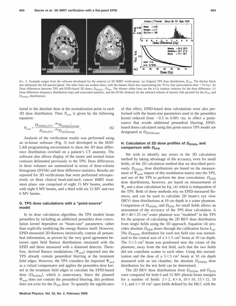
Analysis of the verification results was performed usan in-house softwaresFig. 3d tool developed in the MATLAB programming environment to show the 3D dose difence distribution overlaid on a patient’s CT anatomy.software also allows display of the tumor and normal tiscontours delineated previously in the TPS. Dose differein these volumes are summarized in terms of dose-vohistogramssDVHsd and dose difference statistics. Resultsreported for 3D verifications that were performed retrostively on three clinical head-and-neck cancer IMRT trment plans: one comprised of eight 15 MV beams, anowith eight 6 MV beams, and a third with six 15 MV and tw6 MV beams.

G. TPS dose calculations with a “point-source”model

In its dose calculation algorithm, the TPS models bpenumbra by including an additional penumbra dose colution kernel dependent on “beam-size” parameters, rthan explicitly modifying the energy fluence itself. HowevEPID-measured 2D-fluences intrinsically contain all penbral information, as proven by the very good agreementween open field fluence distributions measured withEPID and those measured with a diamond detector. Tfore, derived fluence modulationssCmodd imported into theTPS already contain penumbral blurring at the treatmfield edges. However, the TPS considers the importedCmod

as a virtual compensator and applies the penumbra dosnel at the treatment field edges to calculate the EPID-bdose sDEPIDflud, which is unnecessary. Since the planCmod does not contain the penumbral blurring, this prob

FIG. 3. Example output from the software developed for the analysisline delineates the left parotid gland. The other lines are isodose lines,Dose differences between TPS and EPID-based 3D doses,DEPIDflu−DTPS. TDose difference frequency distributionstopd and associated statistics, andDEPIDflu distributions.

does not exist for theDTPS dose. To quantify the significance


se

r

-r

-

-

t

r-d

of this effect, EPID-based dose calculations were alsoformed with the beam-size parameters used in the penukernel reduced from,0.5 to 0.001 cm, to effect a poinsource that avoids additional penumbral blurring. EPbased doses calculated using this point-source TPS moddesignated asDEPIDflu/pnt.

H. Calculation of 2D dose profiles of DEPIDflu andcomparison with DEPID

We wish to identify any errors in the 3D calculatmethod by taking advantage of the accuracy, even for sfields, of the 2D calculation method that we described pously. DEPIDflu dose distributions are based on the measment ofCmod, import of this modulation matrix into the TPand use of the TPS to perform the dose convolution.DEPID

dose distributions, however, are based on measuremeCp and a dose calculation by Eq.s4d which is independent othe TPS. Both of these methods rely on EPID-measuredences, and can be used to calculate 2D beam’s eyesBEVd dose distributions at 10 cm depth in a water phanComparison ofDEPIDflu andDEPID for small fields allows aassessment of the accuracy of the TPS dose calculati40340325 cm3 water phantom was “modeled” in the Tfor the purpose of calculating the 2D BEV dose distribufrom single fields using the 3D approach. Equations4d pro-vides absoluteDEPID doses through the calibration factorkcal.The DEPIDflu distribution for each test field size was normized to the central axis of a 535 cm2 beam at 10 cm deptThe 535 cm2 beam was positioned near the corner ofphantom, away from the test field, such that the two fidid not contribute scatter to each other. Using this norization and the dose of a 535 cm2 beam at 10 cm depmeasured with an ion chamber, the absoluteDEPIDflu dosedistribution for the test field can be determined.

The 2D BEV dose distributions fromDEPIDflu and DEPID

were compared for both 6 and 15 MV photon beam enefor a number of fields: 232, 434, 10310, 15315, 10

2

IMRT verifications.sad Original TPS dose distribution,DTPS. The thicker blacthe thinner black line representing the 70 Gy linesprescription dose =74 Gyd. sbdinner white lines are the 4 Gy isodose contours for the dose differenscd

DVHssbottomd for the selected volume of interestsleft parotidd for theDTPSand

of 3Dwithhe ththe

31, and 1310 cm open fields defined by the MLC with the

tof

ionlate

forfor

s bema

e camed

iondure-as

RTopo

thedarn-s. 19dedureonsTh

dose

em-glarownan-

nel

e 1nel, fae 1e retroneralelsof

re:

ol-vely.dia-

olu-ordose-

cm


secondary collimators set to 20320 cm2; a single segmenof a step-and-shoot IMRT field; and the entire IMRT fieldsthe three treatment plans for which a 3D IMRT verificatwas performed. The EPID images, required to calcuDEPIDflu and DEPID, were acquired using 40 MUs/ imagethe open and IMRT-segment fields, and 100 MUs/ imagethe multisegment IMRT fieldssall at 100 MU/mind. In orderto determine the combined effects of the discrepancietween both the measured and TPS-optimized modulationtrix, and the TPS-independent and TPS-dependent dosculations, a similar set of 2D comparisons were perforbetweenDEPID andDTPS.

I. Comparison of 3D EPID-based doses to TLDmeasurements

For further validation, our 3D EPID-based verificattechnique was compared to an IMRT verification proceemploying thermoluminescent dosimetersTLDd dose measurements. The latter verification had been performedrequirement for participation in an IMRT protocolsRTOGH-0022d, and involved generating and delivering an IMtreatment plan for a hypothetical treatment of an anthrmorphic head and neck phantom. A dosimetry insert forphantom contains regions describing primary, seconPTVs, and a critical structure.sFurther details of this phatom and the verification procedures can be found in Refand 20.d After irradiation of the phantom, the doses recorby the TLDs placed in each of these regions were measby the RPCsRadiological Physics Center, M.D. AndersCancer Center, Houston, TXd. The locations of the TLDwere also delineated on the CT scan of the phantom.TLD doses were compared to the corresponding meancalculated by the TPS using the EPID-measuredCmod andthe TPS-optimizedCmod.

III. RESULTS

A. Monte Carlo generated kernels

The Monte Carlo generated EPID initial dose kernel,pirical backscatter-glare kernel, and the combined dose-kernel used in restoring the 6 MV aS500 images are shin Fig. 4. All kernels were scored over the entire EPID phtom, which spans 30 cm. The “IMRT BEV phantom” kerKphantom

6MV used in Eq.s4d is shown in Fig. 5.The combined dose-glare kernels for both the 6 and th

MV Linac spectrums are shown in Fig. 6. The 6 MV keris much narrower near the incident beamlet, howeveraway, it has a much larger magnitude compared to thMV kernel. This is expected, since near the beamlet thsponse is dominated by the range of the liberated elecfrom primary interactions, and in the far-range by latphoton scattering. The shape of these dose-glare kernwell described by the following function, which is the sum
five exponential terms:

--l-

a

-

y

d

es

e

5

r5-s

is

Kdose-glaresrd = exps− a1rd + a2exps− a3rd + a4exps− a5rd

+ a6exps− a7rd + a8exps− a9rd. s7d

The best-fit parameters for the 6 MV kernel aa1=23.35 cm−1, a2=1.727310−3, a3=2.620 cm−1,a4=1.160310−4, a5=0.5367 cm−1, a6=5.571310−6, a7

=0.054 20 cm−1, a8=5.783310−8 a9=0.009 293 cm−1;for the 15 MV kernel they are:a1=17.63 cm−1, a2=6.057310−3, a3=2.367 cm−1, a4=9.195310−5, a5=0.4038 cm−1,a6=4.194310−7, a7=0.020 21 cm−1, a8=9.471310−8, a9

=0.001 179 cm−1.

B. Fluence profiles from the aS500 EPID anddiamond detector scans

Cross-plane scans using 6 MV photons, for 10310 cm2

and 434 cm2 photon fields collimated by the secondary climators and the MLC are seen in Figs. 7 and 8, respectiThe solid lines show in-air profiles measured using a

FIG. 4. The radially symmetric 6 MV kernels used in the EPID deconvtion: the Monte Carlo generated initial dose kernelsscored in the phosphscreend, the empirically generated backglare kernel, and the combinedglare kernel.

FIG. 5. The radially symmetric 6 MV IMRT BEV phantom kernel at 10
depth.

idenraw

andctedthe

ails,orn

r-thade

tedectos thveete

alsoeg-MVofent

EPIDenceially6eree of, dia-me-der-er-patialide of

d 15

then are


mond detector with a brass buildup caps1.1 cm diameterd. Itis assumed that these profiles are proportional to the incenergy fluence. The dashed lines show profiles of theEPID image acquired using the aS500 in IMRT mode,the dotted lines show profiles of the EPID image correusing Eq.s3d. Compared to the diamond fluence profiles,raw EPID profiles are much larger in the penumbral trounded in the penumbra itself, and do not show the hcaused by the flattening filter. Field sizes of 232 cm2, 434 cm2, 10310 cm2, and 20320 cm2 were used to detemine the parameters of the backscatter-glare kernelminimized the difference between diamond detector andconvolved profiles in the penumbra tails. EPID correcprofiles are in excellent agreement with the diamond detscans, including penumbra tails and edges, as well aprofile horns. The diamond energy fluence scans haslightly smoother penumbra because of the 1.1 cm diambrass buildup cap and the 2.2 mmssensitive volumed diam-eter diamond detector.

FIG. 6. The radially symmetric combined dose-glare kernels for 6 anMV Linac spectrums.

FIG. 7. Cross-plane scans for a 6 MV, 10310 cm2 in-air field taken with adiamond detector, the raw EPID, and the final correctedsfluenced EPID
image.

t

s

t-

rear

Fluence profiles obtained from the aS500 image weretested using small fields commonly found in IMRT sments. Figure 9 shows one segment from a clinical 6IMRT field, where the dotted line indicates the locationthe profile shown in Fig. 10. For all subfields in the segmfranging from 0.5 cmssubfield 1d to 2.5 cm ssubfield 2dg,fluences are accurately measured using the correctedimage. This segment delivers a sharp, nearly constant fluwithin open subfields, while the fluence drops substantin the near-penumbra regionsbetween subfields 5 andd.Ideally, we would expect this type of fluence profile, whthe peak heights vary only slightly due to the horn shapan open-field fluence. Because of the buildup cap usedmond detector profiles are not as sharp, and voluaveraging effects cause small subfields to be unrepresentedssubfield 1d, and penumbra regions to be ovrepresented. Raw EPID profiles have an even poorer sresponse, and severely over-represent the fluence outsthe open subfields.

FIG. 8. Cross-plane scans for a 6 MV, 434 cm2 in-air field taken with adiamond detector, the raw EPID, and the final correctedsfluenced EPIDimage.

FIG. 9. One segment from a clinical IMRT field. The dotted line showslocation of the measured scan/profiles. Small subfields within the sca
numbered.

2Daret in15f thecom-

s ofral

eeter

fined

de-l

subfields in the scan are numbered.

hoton

v.

v.



C. Comparisons of 2D dose distributions:DEPIDflu , DEPIDflu/pnt , DEPID, and DTPS

1. Open fields and IMRT-segment field

Comparisons of the different methods of calculatingdose distributions at 10 cm depth in a water phantomsummarized for open fields and a single IMRT segmenTables Isad and Isbd for incident photon energies of 6 andMV, respectively. The means and standard deviations o2D dose difference maps are calculated for the threeparisons: DEPIDflu−DEPID, DTPS−DEPID, and DEPIDflu/pnt

−DEPID. These statistics are calculated for two regioninterest sROIsd: a ROI sROI1d encompassing the centquarter of the open fields—e.g., the central 535 cm2 for the10310 cm2 field; and a second ROIsROI2d that includes thentire field and its penumbra, and is described by a perimpositioned 0.5 cm outside the nominal field edge as de

10 cm depth in a water phantom:DEPIDflu sEPID Cmod, TPS convolutiond, DTPS

point” sourced, andDEPID sEPID Cmod, TPS-independent convolutiond. Meanose are calculated for two ROIs and a number of different fields for p

DEPIDflu−DEPID DTPS−DEPID DEPIDflu/pnt−DEPID

ean Std. dev. Mean Std. dev. Mean Std. des%d s%d s%d s%d s%d s%d

0.2 0.3 0.2 0.5 0.2 0.3−0.1 0.5 0.1 0.6 −0.1 0.5−1.1 0.3 1.5 0.4 −1.1 0.3−1.6 0.3 4.8 0.3 −1.5 0.3−1.7 1.1 5.9 1.2 −0.5 0.8−0.5 0.6 −3.9 1.8 0.0 0.5

1.4 1.7 0.2 5.3 1.4 1.40.9 1.9 0.2 4.5 0.9 1.4

−0.4 2.9 0.4 5.0 −0.4 1.9−0.6 3.7 −4.5 9.7 −0.5 2.5−0.4 4.4 3.0 6.0 −0.3 3.0−0.1 3.4 −16.2 11.4 0.0 2.1

0.5 3.3 1.1 6.3 0.6 2.1

DEPIDflu−DEPID DTPS−DEPID DEPIDflu/pnt−DEPID

ean Std. dev. Mean Std. dev. Mean Std. des%d s%d s%d s%d s%d s%d

−1.1 0.6 −1.2 0.7 −1.1 0.6−1.2 0.2 −1.1 0.3 −1.2 0.2−0.6 0.4 0.1 0.7 −0.6 0.4

2.4 1.0 3.7 1.8 2.7 0.7−0.8 1.6 3.7 1.2 0.4 1.6

1.4 0.9 −10.6 2.0 2.1 0.8

−0.2 1.9 −1.9 5.4 −0.2 1.70.2 2.2 −1.1 4.6 0.2 2.0

−0.1 2.8 −0.7 4.9 0.0 2.40.6 3.5 −4.8 8.4 0.7 3.00.6 3.8 3.3 6.2 0.7 3.00.9 4.1 −17.4 9.3 1.0 3.8−0.1 3.9 −0.3 6.0 0.0 2.9

FIG. 10. Scan profiles from a clinical IMRT segment, from a diamondtector, the raw EPID, and the deconvolved EPIDsfluenced image. Smal

TABLE I. Statistical comparison of different methods of calculating dose atsTPSCmod, TPS convolutiond, DEPIDflu/pnt sEPID Cmod, TPS convolution with a “dose differences and standard deviations as percentages of the maximumDEPID dbeam energies ofsad 6 andsbd 15 MV.

(a) 6 MV

Field MROI scm2d

ROI1: central quarter of field area 153151031043423210311310

ROI2: entire field and penumbra 153151031043423210311310

IMRT segment

(b) 15 MV

Field MROI scm2d

ROI1: central quarter of field area 153151031043423210311310

ROI2: entire field and penumbra 153151031043423210311310

IMRT segment

orte

s o

an 2equsfromstsedfroou

rrorsula-for

be-by

enling

ess

iniffer-heeandare

herva

nalo

eaf

-larand

%s

rthe

RT-

pec-e,n thee

hods

forllongroad

S to.

s inlti-lini-

OI2,ean

dose-drd

fe

dif-imummts.


by the MLC. The means and standard deviations are repas a percentage of the maximum in theDEPID dose for thegiven field.

For the larger open field sizes—434, 10310, and 15315 cm2—there is good agreement between all methodcalculating the 2D dose in the central ROIsROI1d, for bothphoton energies. The mean dose differences are less thin all cases, and the standard deviations are less than orto 0.7%. For the larger ROIsROI2d, which also includepenumbral regions, the standard deviations ranging1.7% to 2.9% for theDEPIDflu−DEPID comparison do suggea non-negligible difference between the two EPID-bamethods of calculating dose. These discrepancies arisedifferences between our method of dose convolution andconvolution kernel and those of the TPS; and from any eintroduced in the process of importing the fluence modtion into the TPS. The standard deviations of 4.5%–5.4%DTPS−DEPID indicate a significantly larger disagreementtween the referenceDEPID dose and the dose calculatedthe TPS using TPS-optimizedCmod. This suggests that evfor these relatively large field sizes, the penumbra modeof the TPS is less than ideal.

Differences betweenDTPS and the two EPID-based dosare much more pronounced for the smaller field sizes232, 1031, and 1310 cm2d. The meanDEPIDflu dose differsfrom the meanDEPID dose by at most 2.4% and 0.9%ROI1 and ROI2, respectively. In contrast, mean dose dences betweenDTPS andDEPID are as large as 10.6% in tcentral ROI and 17.4% in the larger ROI2: in ROI1, msDTPS−DEPIDd ranges from −3.9% to 5.9% for 6 MV anfrom −10.6% to 3.7% for 15 MV; in ROI2, these ranges−16.2% to 3.0%s6 MVd and −17.4 to 3.3%s15 MVd. De-ficiencies in the TPS’s modeling of small fields are furtemphasized by the standard deviations in ROI2. Theseues range from 6.0% to 11.4%, much larger than the agous values of 3.4% to 4.4% forDEPIDflu−DEPID. Noteworthyis that the apparent errors inDTPS are much worse when thnarrow dimension of the field is in the direction of MLC le
travel. For example, for the 6 MV case and ROI2, the mean

d

f

%al

mr

l--

dose difference and standard deviation inDTPS−DEPID are−16.2% and 11.4% for the 1310 cm2 field, while only 3.0%and 6.0% for the 1031 cm2 field. Results for the IMRTsegment field, a relatively large field with a highly irregushape, fall in-between those obtained for the smallerlarger open field sizes. The standard deviations of 6.3s6MV d and 6.0%s15 MVd for DTPS−DEPID are not as large afor the 232 and 1310 cm2, but still significantly largethan the corresponding values of 3.3% and 3.9% forDEPIDflu−DEPID comparison.

For the three smaller open field sizes and the IMsegment field, the standard deviation inDEPIDflu/pnt−DEPID ison average 1.2% and 0.6% lower for 6 and 15 MV, restively, in comparison to theDEPIDflu−DEPID case. Thereforthe point-source model improves the agreement betwee2D calculations using Eq.s4d and the 3D calculation of thTPS using the measuredCmod.

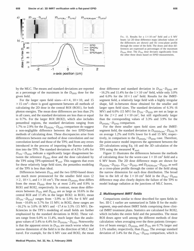
Figure 11 illustrates the differences between the metof calculating dose for the worst-case 1310 cm2 field and a6 MV beam. The 2D dose difference maps are shownDEPIDflu−DEPID, DTPS−DEPID, andDEPIDflu/pnt−DEPID, as welas a cross-plane profile through the center of the field athe narrow dimension for each dose distribution. The bline to the left of the 1310 cm2 field in the DTPS−DEPID

difference map also clearly depicts the failure of the TPmodel leakage radiation at the junctions of MLC leaves

2. Multisegment IMRT fields

Comparisons similar to those described for open fieldSec. III C 1 earlier are summarized in Table II for the musegment, step-and-shoot IMRT fields comprising three ccal IMRT treatment plans. Statistics are calculated for Rwhich includes the entire field and the penumbra. The mROI doses agree well among the different methods ofcalculation: when averaging over the three patientssirrespective of beam energyd, DEPIDflu andDTPS are 0.7% larger an1.1% smaller, respectively, thanDEPID. The average standa

FIG. 11. Results for a 1310 cm2 field and a 6 MVbeam:sad 2D dose difference mapssabsolute values othe differences are shownd and sbd cross-plane profilthrough the center of the field. The doses and doseferences are expressed as percentages of the maxDEPID dose. TheDTPS dose deviates significantly frothe other three doses based on EPID measuremen

deviation of 3.4% for theDTPS−DEPID comparison, which is

p-the

anthronaloe

ri-gredienicalredeLDo

reeareose

r-

s fo-al-

,was

asedenceof they: the

theely.the

are

uc-d topli-

dloy-per-

. 21.the

TCPt Ly-ruchreer-

t intos.eseareded


typical of 2D IMRT verification results at our clinic, is aproximately twice the 1.8% and 1.5% calculated forDEPIDflu−DEPID andDEPIDflu/pnt−DEPID dose differences.

D. Comparison of 3D EPID doses with TLDmeasurements

The TLD dosessDTLDd reported by the RPC afterinverse-planned IMRT treatment was delivered to an anpomorphic head and neck phantom are compared to agousDTPS andDEPIDflu dosessTable IIId. As indicated, theris slightly better agreement with the TLD doses forDEPIDflu

than forDTPS in the low-gradient regions located in the pmary and secondary PTVs, though there is substantial ament between all three doses. However, in the high-graregion where the TLD was placed in the simulated critstructure, theDTPS dose underpredicts the TLD-measudose by 16%. In contrast, theDEPIDflu andDTLD doses agrewithin the RPC-estimated uncertainty of ±3% in the Tdoses. The results usingDEPIDflu/pnt are nearly identical tthose obtained usingDEPIDflu.

E. 3D IMRT verification of clinical IMRT treatmentplans

Results from the retrospective 3D verification of thclinical head-and-neck cancer IMRT treatment planssummarized in Table IV. For each patient, the original ddistribution calculated by the TPS,DTPS, and the dose diffeence distribution,DEPIDflu−DTPS sor DEPIDflu/pnt−DTPSd, arecharacterized by mean and standard deviation statisticfour volumes of interestsVOIsd–PTV, spinal cord, right parotid, and left parotid. The dose distributions were normized such that the median doses in the PTV forDTPSwere 7462, and 71 Gy for patients 1, 2, and 3, respectively. As

TABLE II. Comparisons of different methods of camultisegment IMRT fields comprising three clinicwhich includes the entire field and the penumbra

DEPIDflu−DEP

Patient/No. IMRT fieldsAvg.mean

Avstd.

s%d s%

Patient 1: 8–15 MV fields 0.93 1Patient 2: 8–6 MV fields 0.43 2Patient 3: 6–15 MV, 2–6 MV 0.86 1

TABLE III. Measured TLD dosess±3%d compared tsDTPSd and EPID-measured fluencessDEPIDflu and Dhead and neck phantom.

Region of interestDTPS

sGydDEPIDflu

sGydDEPID

sG

Primary PTV 7.10 7.38 7Secondary PTV 5.63 5.65Critical structure 3.16 3.85


--

e-t

r

found for the head-and-neck phantom, TPS and EPID-bdoses agree well in the PTV, with the mean dose differof 1.4 Gysaveraged over the three patientsd corresponding ta 2% difference. However, in the high-gradient regions ocritical structures, there is once again a large discrepancEPID-based doses are on average 3.7 Gys16%d, 4.4 Gys16%d, and 3.6 Gys12%d higher than the TPS doses forspinal cord, left parotid, and right parotid, respectivDVHs for the PTV and critical structures derived fromTPS and EPID-based dose distributions for patient 3compared in Fig. 12.

F. Radiobiological significance of 3D verificationresults

Differential dose-volume histograms for the critical strture VOIs listed in Table IV were generated and usecalculate radiobiological estimates of normal tissue comcation probabilitiessNTCPsd arising from the TPS anEPID-based dose distributions. NTCP calculations emping the Lyman sigmoidal dose-response model wereformed using software and methods described in RefModel parameter values for both the spinal cord andparotid glands are available from the Burmanet al.22 fits tothe Emamiet al.23 dose-response database; additional Nestimates for the parotids are possible using more recenman model parameter estimates published in Eisbet al.24 and Roesinket al.25 Since large uncertainties acurrently inherent in such radiobiological modeling excises, these calculations are used only to provide insighthe potentialconsequences of TPS dose modeling error

The radiobiological predictions suggest that for ththree treatment plans, the spinal cord is sufficiently spsuch that the additional,4 Gy predicted by the EPID-bas

ting the 2D doses10 cm depth, water phantomd for theRT treatment plans. Statistics are calculated for ROI2,

DTPS−DEPID DEPIDflu/pnt−DEPID

Avg.mean

Avg.std. dev.

Avg.mean

Avg.std. dev.

s%d s%d s%d s%d

−1.14 3.69 0.97 1.39−1.20 3.13 0.51 1.82−1.03 3.43 0.91 1.34

S-calculated doses using fluences modeled by the TPS

/pntd for an IMRT treatment of an anthropomorphic

t DTLD

sGydDTPS

DTLD

DEPIDflu

DTLD

DEPIDflu/pnt

DTLD

7.31 0.97 1.01 1.015.70 0.99 0.99 0.993.76 0.84 1.02 1.03

lculaal IM.

ID

g.dev.d

.68

.07

.67

o TP

EPIDflu

flu/pn

yd

.375.623.86

rate.de-sed

hese-

t 3.

ten-pre-ch

,

sons

ri-

tricana-

S

of


dose for this structure has little impact on the predictedof complication–the NTCP isø2% for all dose distributionsThe NTCP estimates for the parotid glands vary widely,pending on which set of model parameter values are u

The Burmanet al. parameters yield the lowest NTCPs. Tapproximately 4 Gy largerDEPIDflu dose results in an increain the predicted NTCP ofø5% with one exception, the increase from 22% to 40% for the right parotid of patienMuch higher parotid NTCPs result from the more recentsandstatistically basedd parameter estimates. A modest but potially significant increase of between 3% and 13% isdicted with the Roesinket al. parameters, whereas the mu

TABLE IV. 3D IMRT verification results: comparisodose distributions for three clinical IMRT treatme

DTPS DEPIDflu−D

sGyd sGyd

VOI Mean Std. dev. Mean

Patient 1PTV 73.3 5.9 1.9Spinal cord 30.1 9.3 3.8Left parotid 24.0 16.9 4.3Right parotid 29.6 18.1 3.8




.

steeper dose-response described by the Eisbruchet al. pa-rameters lead to NTCP estimates up to 39% higherspatient 3right parotidd when usingDEPIDflu.

Despite the apparent improvement in the 2D compariobtained with the “point-soure” modelsSec. III Cd, the re-sults in Tables III, IV, and V suggest the use ofDEPIDflu/pnt

instead ofDEPIDflu has little practical impact on the 3D vefications.

IV. DISCUSSION

The advantage of 3D IMRT verification is that dosimeuncertainties can be quantified directly with respect to

PSsDTPSd and EPID-basedsDEPIDflu or DEPIDflu/pntd 3Dans.

DEPIDflu/pnt−DTPS DEPIDflu

DTPS

DEPIDflu/pnt

DTPSsGyd

dev. Mean Std. dev. Mean Mean

1.9 1.5 1.03 1.033.7 1.1 1.13 1.124.2 1.8 1.18 1.183.7 1.5 1.13 1.12

1.2 1.1 1.01 1.023.1 1.4 1.20 1.204.2 1.1 1.17 1.182.5 1.7 1.04 1.05

1.6 1.2 1.02 1.024 4.1 1.4 1.15 1.15

4.9 2.5 1.13 1.134.8 1.6 1.20 1.20

FIG. 12. Comparison of DVHs derived from TPsDTPSd and EPID-basedsDEPIDflu or DEPIDflu/pntd dosedistributions generated during 3D IMRT verificationspatient 3’s treatment plan.

n of Tnt pl

TPS

Std.

1.41.11.91.5

1.01.41.21.7

1.21.2.61.6

irectcal-theffi-eamnce

atio

, reingry—thens

Theectcerentsaverion othe-maumu

s toy the

hecal-

lcu-willthe

dthesegradi-hethe

f the

redtion.iredrt-

ap-ac-eam


tomical volumes of interest, making possible a more devaluation of the clinical consequence of errors in TPSculation. By comparison, the information provided bysimpler 2D IMRT verification method is generally insucient for such assessments. At our clinic, our beam-by-b2D verification identifies potential problems by the preseof large “hot” sor “cold”d regions in the 2DDEPID−DTPSdosedifference map, or by mean difference and standard devistatistics for this map that fail specified criteriase.g.,ù2%and 4% for the mean difference and standard deviationspectivelyd. The 2D verification is thus effective at detectlarger errors, including procedural mistakes in the delivee.g., incorrect transfer of MLC leaf sequence file tolinac—and planning—e.g., alignment of MLC leaf junctiowith a critical structure—stages of an IMRT treatment.2D method is ineffective, however, in quantifying the effof smaller errors that, though present, do not arouse conFor example, each field of the three IMRT patient treatm“passed” the 2D verification tests, as supported by theage mean dose difference of −1.1% and standard deviat3.4% reported for these verifications in Table II. Neverless, the results in Tables IV and V indicate that these serrors may lead to considerably larger than expected c

TABLE V. Comparison of radiobiological modelingbasedsDEPIDflu or DEPIDflu/pntd 3D dose distributions

Modelparam.

Ref. No.

NTCP s

VOI DTPS DEPIDflu

Patient 1Spinal cord 22,23 1 2Left parotid 22,23 0 1

25 9 2824 16 22

Right parotid 22,23 4 825 60 7924 30 36


25 12 4524 17 26

Right parotid 22,23 78 8325 100 10024 77 80


25 94 10024 44 56

Right parotid 22,23 1 425 23 6224 21 30

lative dose errors of up to 20% in the critical structures. Such


n

-

n.

-f

ll-

errors may in turn have potential clinical implications athe acceptability of these treatments, as suggested bNTCP analysis summarized in Table V.

One potential limitation of our method of verifying t3D dose distributions calculated by our TPS is that theculation of our EPID-based 3D dosessDEPIDflud relies on theTPS itself to perform the convolution step of the dose calation. Thus, errors introduced in this step by the TPSnot be identified by our verification procedure. However,good agreement between TLDsDTLDd and EPID-basedoses, and the large discrepancy between either ofmeasurement-based doses and the TPS dose in a highent regionssee Table IIId, suggest that a large portion of tdose calculation errors of our TPS are introduced prior toconvolution step, e.g., in the fluence modelling stage ocalculations.

In its current implementation, our 3D method is hampeby the excessive time required to perform the verificaAlthough the time necessary for acquisition of the requEPID images is not longs,1/2 hrd, the process of conveing the EPID-based fluence modulation matrices to thepropriate “compensator” file format, and particularly thetual import of these compensator files on a beam-by-b

dictions of the NTCP based on TPSsDTPSd and EPID-hree clinical IMRT treatment plans.

∆NTCP s%d

EPIDflu/pnt DEPIDflu−DTPS DEPIDflu/pnt−DTPS

2 1 11 1 1

28 20 1922 6 6

9 4 582 19 2337 6 7

0 0 02 2 1

38 32 2625 9 784 5 6

100 0 080 3 3

2 1 140 18 18

100 5 556 13 14

4 3 363 39 4031 10 10

prefor t

%d

D

basis into the TPS is time consuming and tedious. It is an-

ider

od,sed

ng aicalproete. Innceatean

es tS-n-s incal-ical

atecordlma

am-fulsilyods

d Pithe

tionndIn

hishis

msrtal

ty-

f aof

seBiol.

el

ng

ges

ee-Med.

east

n-ld flu-

sing

iga-elec-

nel

arlo-701,

ninePhys.

nell

us

using91.for

tp://

tialMed.

nded.

tic-

n,”

tidtion

s of-neck


ticipated that the 3D method could be streamlined consably on a TPS with a “script-based” user interface.

V. CONCLUSION

As an extension of our previously described 2D methwe have developed a 3D IMRT verification procedure baon measurement of 2D fluence modulation profiles usiflat-panel EPID. Monte Carlo simulations and empirmethods are used to derive deconvolution kernels thatduce excellent agreement between EPID and diamond dtor fluence profiles for both 6 and 15 MV beam energiesour method, 3D doses are calculated using the EPID flueand TPS-dependent convolution. 2D dose profiles in a wphantom and point doses in an anthropomorphic headneck phantom were utilized to compare these 3D dosanalogous doses based on measurementsand completely TPindependentd and those calculated by the TPSsand completely measurement independentd. These comparisons cofirmed the effectiveness of our 3D EPID-based dosequantifying uncertainties in the IMRT dose distributionsculated by the TPS. The 3D verification of three clinIMRT treatment plans suggested that the TPS underestimthe mean doses in the critical structures of the spinaland the parotids by,4 Gy s11%–14%d. Radiobiologicamodeling predictions suggest that such underestimatesbe clinically significant. Thus, if the method can be strelined sufficiently, 3D verification may be a clinically usequality assurance tool that provides information not eaaccessible using more conventional 2D verification meth

ACKNOWLEDGMENTS

This research was supported by Alberta Cancer Boarlot Grant No. R-484. B.W. has also received support inform of studentships from the Alberta Heritage Foundafor Medical Research and the Alberta Cancer Board, aDissertation Fellowship from the University of Alberta.addition, the authors would like to thank Colin Field forexpert assistance with the TMS-Helax TPS, particularlyhelp in generating the point-source TPS calculations.

adElectronic mail: [email protected]. L. Pasmaet al., “Dosimetric verification of intensity modulated beaproduced with dynamic multileaf collimation using an electronic poimaging device,” Med. Phys.26s11d, 2373–2378s1999d.

2J. W. Changet al., “Relative profile and dose verification of intensimodulated radiation therapy,” Int. J. Radiat. Oncol., Biol., Phys.47s1d,231–240s2000d.

3A. Van Eschet al., “Pre-treatment dosimetric verification by means oliquid-filled electronic portal imaging device during dynamic deliveryintensity modulated treatment fields,” Radiother. Oncol.60s2d, 181–190


-

-c-

srdo

d

y

.

-

a

s2001d.4S. C. Vieiraet al., “Dosimetric verification of x-ray fields with steep dogradients using an electronic portal imaging device,” Phys. Med.48s2d, 157–166s2003d.

5B. Warkentin et al., “Dosimetric IMRT verification with a flat-panEPID,” Med. Phys.30s12d, 3143–3155s2003d.

6O. A. Zeidanet al., “Verification of step-and-shoot IMRT delivery usia fast video-based electronic portal imaging device,” Med. Phys.31s3d,463–476s2004d.

7T. R. McNuttet al., “Modeling dose distributions from portal dose imausing the convolution/superposition method,” Med. Phys.23s8d, 1381–1392 s1996d.

8M. Partridge, M. Ebert, and B. M. Hesse, “IMRT verification by thrdimensional dose reconstruction from portal beam measurements,”Phys. 29s8d, 1847–1858s2002d.

9R. J. W. Louweet al., “Three-dimensional dose reconstruction of brcancer treatment using portal imaging,” Med. Phys.30s9d, 2376–2389s2003d.

10W. D. Renneret al., “A dose delivery verification method for convetional and intensity-modulated radiation therapy using measured fieence distributions,” Med. Phys.30s11d, 2996–3005s2003d.

11P. Munro and D. C. Bouius, “X-ray quantum limited portal imaging uamorphous silicon flat-panel arrays,” Med. Phys.25s5d, 689–702s1998d.

12B. M. C. McCurdy, K. Luchka, and S. Pistorius, “Dosimetric investtion and portal dose image prediction using an amorphous silicontronic portal imaging device,” Med. Phys.28s6d, 911–924s2001d.

13Y. El-Mohri et al., “Relative dosimetry using active matrix flat-paimagersAMFPId technology,” Med. Phys.26s8d, 1530–1541s1999d.

14I. Kawrakow and D. W. Rogers, “The EGSnrc code system: Monte Csimulation of electron and photon transport,” NRCC Report PIRSNRC Canada, 2002.

15D. Sheikh-Bagheri and D. W. Rogers, “Monte Carlo calculation ofmegavoltage photon beam spectra using the BEAM code,” Med.29s3d, 391–402s2002d.

16J. O. Kimet al., “A Monte Carlo model of an amorphous silicon flat paimager for portal dose prediction,” presented at the7th InternationaWorkshop on Electronic Portal Imaging, Vancouver, Canada, 2002.

17J. V. Sieberset al., “Monte Carlo computation of dosimetric amorphosilicon electronic portal images,” Med. Phys.31s7d, 2135–2146s2004d.

18A. Ahnesjo, “Dose calculation methods in photon beam therapyenergy deposition kernels,” Ph.D. Thesis, Stockholm University, 19

19G. Ibbott et al., “An anthropomorphic head and neck phantomevaluation of intensity modulated radiation therapy,” htrpc.mdanderson.org/rpc, 2002.

20P. Cadmanet al., “Dosimetric considerations for validation of a sequenIMRT process with a commercial treatment planning system,” Phys.Biol. 47s16d, 3001–3010s2002d.

21B. Warkentinet al., “A TCP-NTCP estimation module using DVHs aknown radiobiological models and parameter sets,” J. Appl. Clin. MPhys. 5s1d, 50–63s2004d.

22C. Burmanet al., “Fitting of normal tissue tolerance data to an analyfunction,” Int. J. Radiat. Oncol., Biol., Phys.21s1d, 123–135s1991d.

23B. Emamiet al., “Tolerance of normal tissue to therapeutic irradiatioInt. J. Radiat. Oncol., Biol., Phys.21s1d, 109–122s1991d.

24A. Eisbruchet al., “Dose, volume, and function relationships in parosalivary glands following conformal and intensity-modulated irradiaof head and neck cancer,” Int. J. Radiat. Oncol., Biol., Phys.45s3d, 577–587 s1999d.

25J. M. Roesinket al., “Quantitative dose-volume response analysichanges in parotid gland function after radiotherapy in the head-and
region,” Int. J. Radiat. Oncol., Biol., Phys.51s4d, 938–946s2001d.

three-dimensional imrt veriﬁcation with a ﬂat-panel epidlcr.uerj.br/manual_abfm/three...

Documents