Proceedings World Geothermal Congress 2015

Melbourne, Australia, 19-25 April 2015

1

Three-Dimensional Resistivity Structure of the Yanaizu-Nishiyama Geothermal Reservoir,

Northern Japan

Toshihiro Uchida1, Shinichi Takakura

1, Takumi Ueda

1, Tatsuya Sato

2, and Yasuyuki Abe

3

1Geological Survey of Japan, AIST, 2Geothermal Energy Research and Development, 3Okuaizu Geothermal

AIST Tsukuba Central 7, Tsukuba, 305-8567, Japan

uchida-toshihiro@aist.go.jp

Keywords: magnetotelluric survey, 3D inversion, resistivity, geothermal reservoir, Yanaizu-Nishiyama

ABSTRACT

We conducted three-dimensional (3D) magnetotelluric (MT) survey in the Yanaizu-Nishiyama geothermal field, Fukushima

Prefecture, northern Japan, where a 65 MWe geothermal power plant has been in operation since 1995. The purpose of the survey

was to obtain a detailed electrical resistivity structure of the geothermal reservoir in three dimensions in order to provide

information for selecting appropriate location for drilling of additional production wells. The 3D MT measurement was carried out

at 30 locations in 2010. In addition to them, we utilized existing MT data obtained for a 2D MT survey by the Geological Survey of

Japan, AIST, in 2000 and 2001 for a regional geophysical study. Two subsets of MT data were prepared for 3D interpretation. The

first subset (Area-1), consisting of 51 MT stations with impedance rotation of N35°W, densely covers the main geothermal field.

For the second subset (Area-2), eight outer stations were added to the first subset, with changing the rotation direction to 0 degree.

This is to examine how the inversion result differs when we set different survey coverage over the target area. The resistivity

models obtained by 3D inversion indicate clear upper and lower boundaries of the low-resistivity cap layer over the geothermal

reservoir. Distribution of feed zones recognized in production boreholes is confined below the lower boundary of the low-resistivity

clay cap. The shape of the low-resistivity layer also shows a good correlation with a low-temperature zone in the distribution of

underground temperature. The 3D model of Area-1 shows high-resistivity anomalies along the northern and southern edges of the

interpretation zone at depth from 1 km to 3 km. On the other hand, Area-2 does not show such anomalies at the locations in Area-1.

This indicates that the survey area should be sufficiently wider than the zone of interpretation in order not to produce artifacts

caused by an anomalous structure at the edge of the target area.

1. INTRODUCTION

The Yanaizu-Nishiyama geothermal power plant started its operation in 1995 with an installed capacity of 65 MWe. The steam

production is run by Okuaizu Geothermal, Co., Ltd. (OAG), while the power generation and distribution are operated by Tohoku

Electric Power Co., Inc. The running capacity dropped several years after the inauguration and has been below 50 MWe since 2010.

According to OAG, the reservoir evaluation conducted before the installation seemed to be optimistic as compared with the real

capacity of the reservoir. Under such circumstances, in order to investigate detailed reservoir structure of the field and to seek for

valid information for selecting locations for make-up drillings, a 3D MT survey was conducted in 2010 under a joint research

project among Tohoku Electric Power, OAG and AIST. The only intensive electromagnetic survey applied over the geothermal

field before the exploitation was long-offset time-domain electromagnetics (LOTEM) with 1D interpretation (Nitta et al., 1987). In

addition, electrical logging was not performed in most of production and injection wells during the exploitation stage. Therefore,

electrical resistivity structure has not been studied well in the area. The aim of the 2010 MT survey was to provide a reliable 3D

resistivity model for understanding the reservoir structure.

2. MT DATA

The main survey area, for which we planned to construct a 3D model, is approximately 3.5 km x 3.5 km in size, shown as Area-1 in

Fig.1. The Yanaizu-Nishiyama geothermal field is located in a small caldera that was formed approximately 300,000 years ago

(Mizugaki, 2000). The local geological strike is approximately in the NW-SE direction, if we follow the direction of main faults in

the field. These faults are estimated to act as conduits for hydrothermal circulation and form a reservoir system (Nitta et al., 1987).

AIST conducted MT measurement covering a wider area of Yanaizu-Nishiyama field for 2D interpretation in 2000 and 2001 under

a geothermal technology research project. We re-processed all of the time series data in this work. Then, we arranged new MT

stations to make a grid-like array in Area-1, by utilizing these existing MT stations, in the MT survey in 2010. The number of MT

stations obtained in 2010 was 30. An average station interval was approximately 500 m in Area-1, although we moved most of the

stations in the mountain area to avoid steep terrain change or so. The remote reference site was located approximately 200 km away

in northern Honshu Island.

A DC train system is operated near the survey area. The nearest train station is about 20 km southeast from the area. Therefore,

noisy waveforms caused by frequent load changes of the DC railway were observed at all stations. Also, the geothermal power

plant, located in the center of the survey area, was in operation throughout the survey period. Although we ran data acquisition at

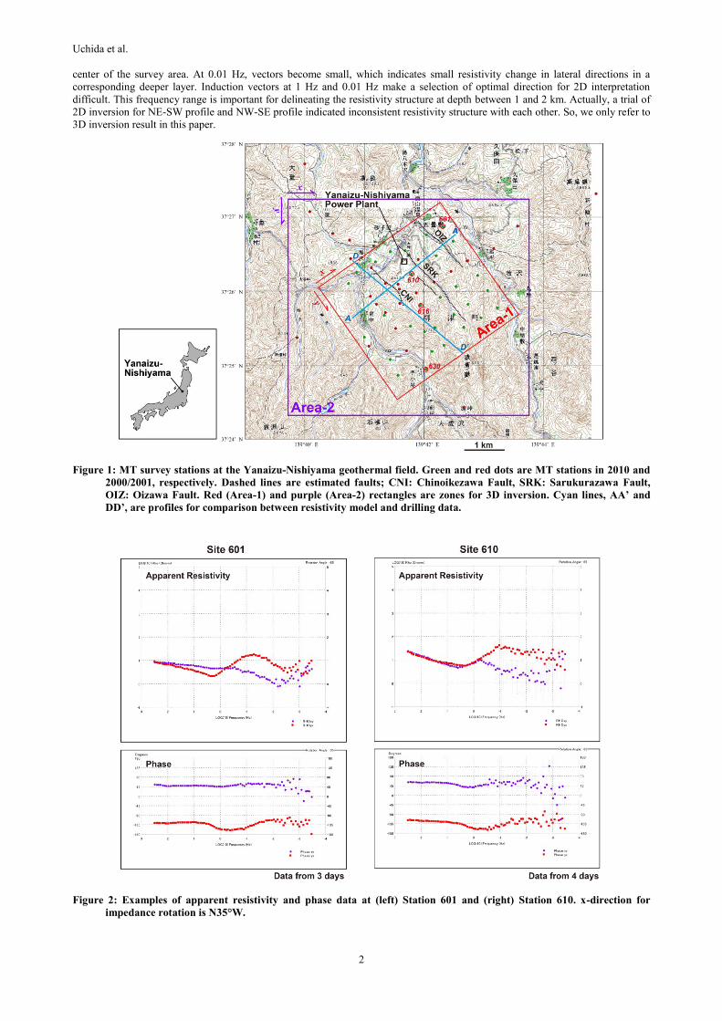
least for three days at each site (maximum of six days), average quality of the processed data was not very good. Examples of

typical good and bad data are shown in Fig. 2. Station 601 is close to a local village, but the data quality is one of the best among all

stations. Station 610, located between the turbine building and one of the well pads, is one of the worst quality stations. Even so,

high frequency data above about 0.3 Hz is generally clean for all stations.

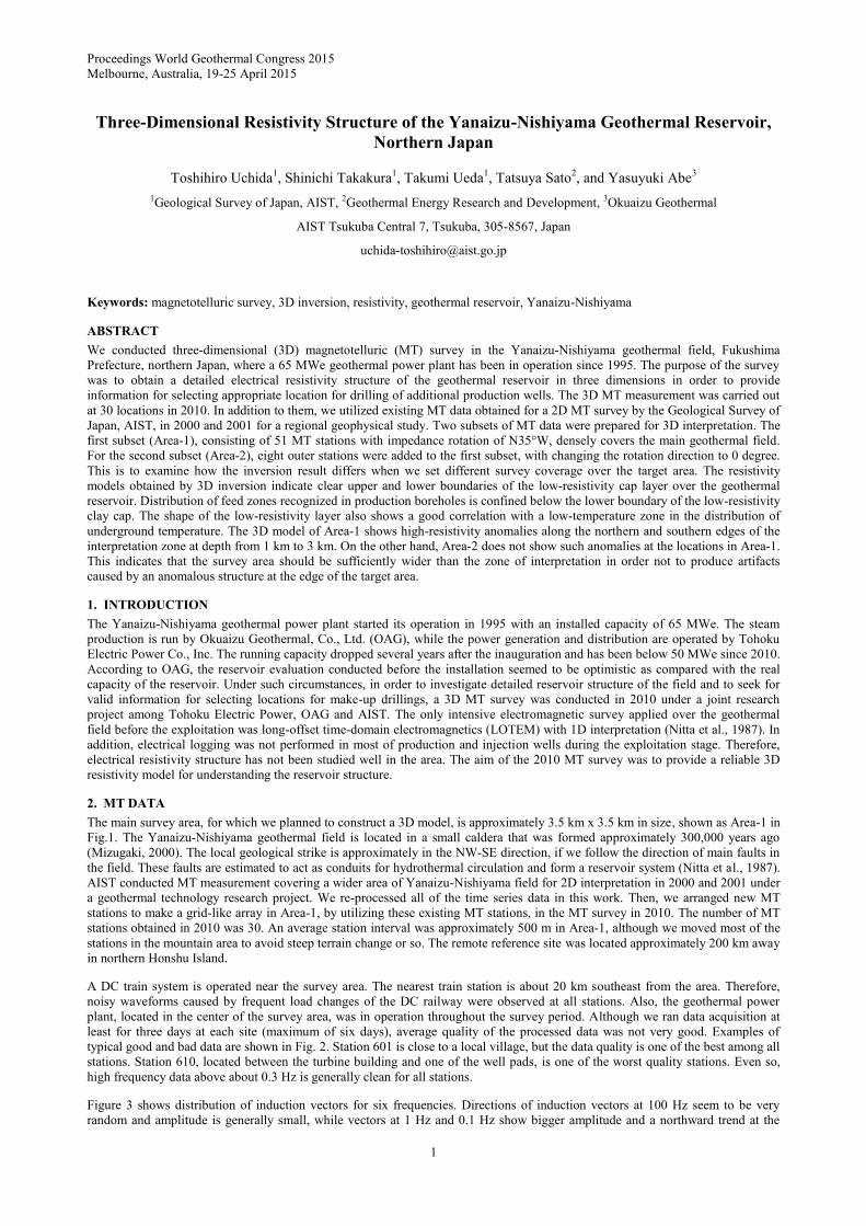
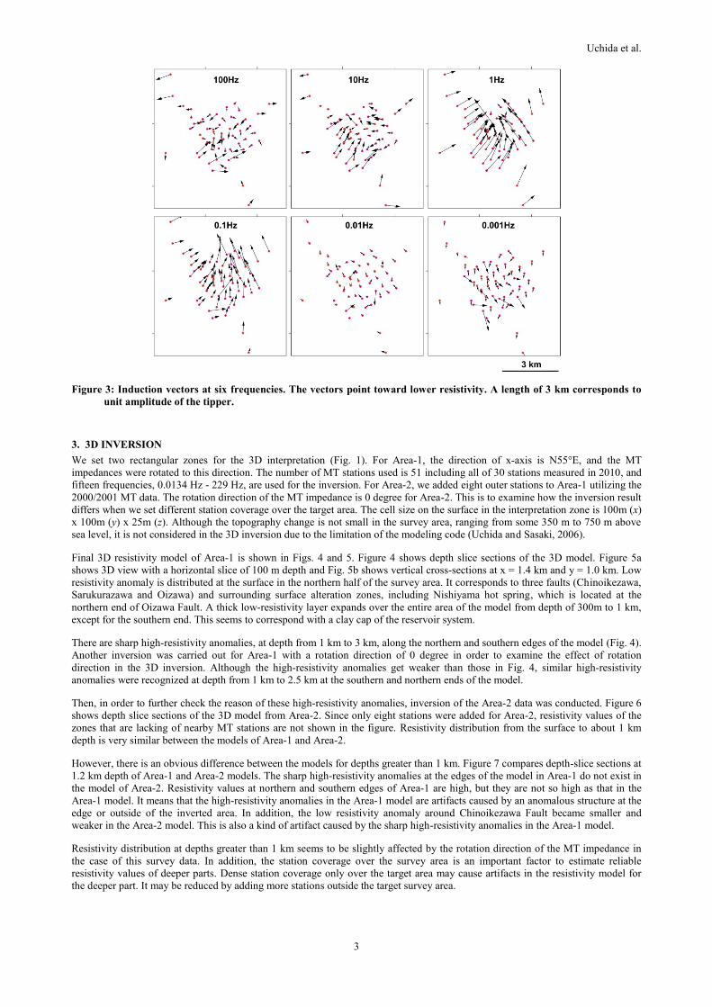
Figure 3 shows distribution of induction vectors for six frequencies. Directions of induction vectors at 100 Hz seem to be very

random and amplitude is generally small, while vectors at 1 Hz and 0.1 Hz show bigger amplitude and a northward trend at the

Uchida et al.

2

center of the survey area. At 0.01 Hz, vectors become small, which indicates small resistivity change in lateral directions in a

corresponding deeper layer. Induction vectors at 1 Hz and 0.01 Hz make a selection of optimal direction for 2D interpretation

difficult. This frequency range is important for delineating the resistivity structure at depth between 1 and 2 km. Actually, a trial of

2D inversion for NE-SW profile and NW-SE profile indicated inconsistent resistivity structure with each other. So, we only refer to

3D inversion result in this paper.

Figure 1: MT survey stations at the Yanaizu-Nishiyama geothermal field. Green and red dots are MT stations in 2010 and

2000/2001, respectively. Dashed lines are estimated faults; CNI: Chinoikezawa Fault, SRK: Sarukurazawa Fault,

OIZ: Oizawa Fault. Red (Area-1) and purple (Area-2) rectangles are zones for 3D inversion. Cyan lines, AA’ and

DD’, are profiles for comparison between resistivity model and drilling data.

Figure 2: Examples of apparent resistivity and phase data at (left) Station 601 and (right) Station 610. x-direction for

impedance rotation is N35°W.

Uchida et al.

3

Figure 3: Induction vectors at six frequencies. The vectors point toward lower resistivity. A length of 3 km corresponds to

unit amplitude of the tipper.

3. 3D INVERSION

We set two rectangular zones for the 3D interpretation (Fig. 1). For Area-1, the direction of x-axis is N55°E, and the MT

impedances were rotated to this direction. The number of MT stations used is 51 including all of 30 stations measured in 2010, and

fifteen frequencies, 0.0134 Hz - 229 Hz, are used for the inversion. For Area-2, we added eight outer stations to Area-1 utilizing the

2000/2001 MT data. The rotation direction of the MT impedance is 0 degree for Area-2. This is to examine how the inversion result

differs when we set different station coverage over the target area. The cell size on the surface in the interpretation zone is 100m (x)

x 100m (y) x 25m (z). Although the topography change is not small in the survey area, ranging from some 350 m to 750 m above

sea level, it is not considered in the 3D inversion due to the limitation of the modeling code (Uchida and Sasaki, 2006).

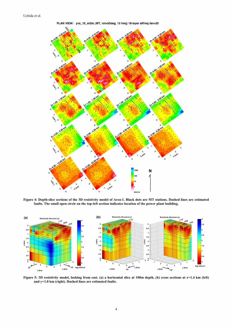
Final 3D resistivity model of Area-1 is shown in Figs. 4 and 5. Figure 4 shows depth slice sections of the 3D model. Figure 5a

shows 3D view with a horizontal slice of 100 m depth and Fig. 5b shows vertical cross-sections at x = 1.4 km and y = 1.0 km. Low

resistivity anomaly is distributed at the surface in the northern half of the survey area. It corresponds to three faults (Chinoikezawa,

Sarukurazawa and Oizawa) and surrounding surface alteration zones, including Nishiyama hot spring, which is located at the

northern end of Oizawa Fault. A thick low-resistivity layer expands over the entire area of the model from depth of 300m to 1 km,

except for the southern end. This seems to correspond with a clay cap of the reservoir system.

There are sharp high-resistivity anomalies, at depth from 1 km to 3 km, along the northern and southern edges of the model (Fig. 4).

Another inversion was carried out for Area-1 with a rotation direction of 0 degree in order to examine the effect of rotation

direction in the 3D inversion. Although the high-resistivity anomalies get weaker than those in Fig. 4, similar high-resistivity

anomalies were recognized at depth from 1 km to 2.5 km at the southern and northern ends of the model.

Then, in order to further check the reason of these high-resistivity anomalies, inversion of the Area-2 data was conducted. Figure 6

shows depth slice sections of the 3D model from Area-2. Since only eight stations were added for Area-2, resistivity values of the

zones that are lacking of nearby MT stations are not shown in the figure. Resistivity distribution from the surface to about 1 km

depth is very similar between the models of Area-1 and Area-2.

However, there is an obvious difference between the models for depths greater than 1 km. Figure 7 compares depth-slice sections at

1.2 km depth of Area-1 and Area-2 models. The sharp high-resistivity anomalies at the edges of the model in Area-1 do not exist in

the model of Area-2. Resistivity values at northern and southern edges of Area-1 are high, but they are not so high as that in the

Area-1 model. It means that the high-resistivity anomalies in the Area-1 model are artifacts caused by an anomalous structure at the

edge or outside of the inverted area. In addition, the low resistivity anomaly around Chinoikezawa Fault became smaller and

weaker in the Area-2 model. This is also a kind of artifact caused by the sharp high-resistivity anomalies in the Area-1 model.

Resistivity distribution at depths greater than 1 km seems to be slightly affected by the rotation direction of the MT impedance in

the case of this survey data. In addition, the station coverage over the survey area is an important factor to estimate reliable

resistivity values of deeper parts. Dense station coverage only over the target area may cause artifacts in the resistivity model for

the deeper part. It may be reduced by adding more stations outside the target survey area.

Uchida et al.

4

Figure 4: Depth-slice sections of the 3D resistivity model of Area-1. Black dots are MT stations. Dashed lines are estimated

faults. The small open circle on the top-left section indicates location of the power plant building.

Figure 5: 3D resistivity model, looking from east. (a) a horizontal slice at 100m depth, (b) cross sections at x=1.4 km (left)

and y=1.0 km (right). Dashed lines are estimated faults.

Uchida et al.

5

Figure 6: Depth-slice sections of the 3D resistivity model of Area-2. Black rectangles correspond to the zone of Area-1 in

Fig. 4.

Figure 7: Comparison of depth-slice sections at 1.2 km depth of (a) Area-1 and (b) Area-2 models. Dashed lines are location

of estimated faults at the surface.

Uchida et al.

6

4. INTERPRETATION

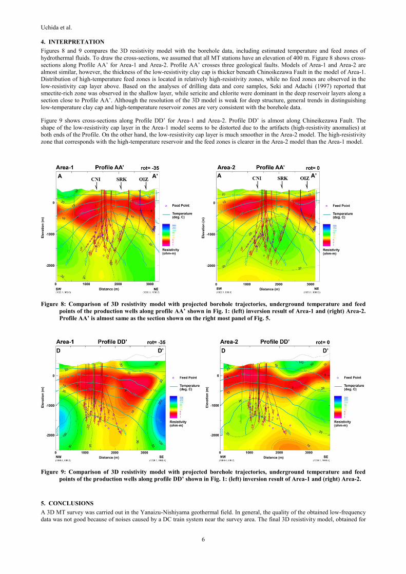
Figures 8 and 9 compares the 3D resistivity model with the borehole data, including estimated temperature and feed zones of

hydrothermal fluids. To draw the cross-sections, we assumed that all MT stations have an elevation of 400 m. Figure 8 shows cross-

sections along Profile AA’ for Area-1 and Area-2. Profile AA’ crosses three geological faults. Models of Area-1 and Area-2 are

almost similar, however, the thickness of the low-resistivity clay cap is thicker beneath Chinoikezawa Fault in the model of Area-1.

Distribution of high-temperature feed zones is located in relatively high-resistivity zones, while no feed zones are observed in the

low-resistivity cap layer above. Based on the analyses of drilling data and core samples, Seki and Adachi (1997) reported that

smectite-rich zone was observed in the shallow layer, while sericite and chlorite were dominant in the deep reservoir layers along a

section close to Profile AA’. Although the resolution of the 3D model is weak for deep structure, general trends in distinguishing

low-temperature clay cap and high-temperature reservoir zones are very consistent with the borehole data.

Figure 9 shows cross-sections along Profile DD’ for Area-1 and Area-2. Profile DD’ is almost along Chineikezawa Fault. The

shape of the low-resistivity cap layer in the Area-1 model seems to be distorted due to the artifacts (high-resistivity anomalies) at

both ends of the Profile. On the other hand, the low-resistivity cap layer is much smoother in the Area-2 model. The high-resistivity

zone that corresponds with the high-temperature reservoir and the feed zones is clearer in the Area-2 model than the Area-1 model.

Figure 8: Comparison of 3D resistivity model with projected borehole trajectories, underground temperature and feed

points of the production wells along profile AA’ shown in Fig. 1: (left) inversion result of Area-1 and (right) Area-2.

Profile AA’ is almost same as the section shown on the right most panel of Fig. 5.

Figure 9: Comparison of 3D resistivity model with projected borehole trajectories, underground temperature and feed

points of the production wells along profile DD’ shown in Fig. 1: (left) inversion result of Area-1 and (right) Area-2.

5. CONCLUSIONS

A 3D MT survey was carried out in the Yanaizu-Nishiyama geothermal field. In general, the quality of the obtained low-frequency

data was not good because of noises caused by a DC train system near the survey area. The final 3D resistivity model, obtained for

Uchida et al.

7

the first time in the field, showed clear image of low-resistivity clay cap and high-resistivity hydrothermal reservoir. These

interpretations are also very consistent with borehole data compiled by Okuaizu Geothermal, Co., Ltd.

The MT stations were arranged to densely cover the survey area over the geothermal field. However, the inversion result that

utilized the dense MT stations produced artifacts along the edge of the interpretation zone. Such artifacts can be avoided by adding

several MT stations outside the survey area. Inclusion of the outside MT stations in the 3D inversion can reduce the artifacts caused

by anomalous structure that exists at the edge or just outside of the target area.

REFERENCES

Mizugaki, K., Geologic structure and volcanic history of the Yanaizu-Nishiyama (Okuaizu) geothermal field, Northeast Japan,

Geothermics, 29, (2000), 233-256.

Nitta, T., Suga, S., Tsukagoshi, S., and Adachi, M., Geothermal resources in the Okuaizu, Tohoku district, Japan (In Japanese with

English abstract), Chinetsu, 24, (1987), 26-56.

Seki, Y., and Adachi, M., Stratigraphy and hydrothermal alteration based on well data from Okuaizu geothermal system, Japan,

Bull. Geol. Surv. Japan, 48, (1997), 365-412.

Uchida, T., and Sasaki, Y., Stable 3-D inversion of MT data and its application to geothermal exploration, Exploration Geophysics,

37, (2006), 223-230.