three-dimensional drawingscs.brown.edu/~rt/gdhandbook/chapters/3d.pdf · three-dimensional drawings...

14Three-Dimensional Drawings

Vida DujmovicCarleton University

Sue WhitesidesUniversity of Victoria

14.1 Introduction . . . . . . . . . . . . . . . . . . . . . . . . . . . . . . . . . . . . . . . . . . . . . . . . . 45514.2 Straight-line and Polyline Grid Drawings . . . . . . . . . . . . . . . 457

Straight-line grid drawings • Upward • Polyline

14.3 Orthogonal Grid Drawings . . . . . . . . . . . . . . . . . . . . . . . . . . . . . . . . 466Point-drawings • Box-drawings

14.4 Thickness . . . . . . . . . . . . . . . . . . . . . . . . . . . . . . . . . . . . . . . . . . . . . . . . . . . . 47314.5 Other (Non-Grid) 3D Drawing Conventions . . . . . . . . . . . . 477References . . . . . . . . . . . . . . . . . . . . . . . . . . . . . . . . . . . . . . . . . . . . . . . . . . . . . . . . . . 482

14.1 Introduction

Two-dimensional graph drawing, that is, graph drawing in the plane, has been widelystudied. While this is not yet the case for graph drawing in 3D, there is nevertheless agrowing body of research on this topic, motivated in part by advances in hardware forthree-dimensional graphics, by experimental evidence suggesting that displaying a graphin three dimensions has some advantages over 2D displays [WF94, WF96, WM08], and byapplications in information visualization [WF94, WM08], VLSI circuit design [LR86], andsoftware engineering [WHF93]. Furthermore, emerging technologies for the nano throughmicro scale may create demand for 3D layouts whose design criteria depend on, and varywith, these new technologies.

Not surprisingly, the mathematical literature is a source of results that can be regardedas early contributions to graph drawing. For example, a theorem of Steinitz states that agraph G is a skeleton of a convex polyhedron if and only if G is a simple 3-connected planargraph.

It is natural to generalize from drawing graphs in the plane to drawing graphs on othersurfaces, such as the torus. Indeed, surface embeddings are the object of a vast amount ofresearch in topological graph theory, with entire books devoted to the topic. We refer theinterested reader to the book by Mohar and Thomassen [MT01] as an example.

Numerous drawing styles or conventions for 3D drawings have been studied. These stylesdiffer from one another in the way they represent vertices and edges. We focus on the mostcommon ones and on the algorithms with provable bounds on layout properties and runningtime.

In this chapter, by a drawing we always mean a graph representation (realization, layout,embedding) where no two vertices overlap and no vertex-edge intersections occur unlessthere is a corresponding vertex-edge incidence in the combinatorial graph. We say that twoedges cross if they intersect at a point that is not the location of a shared endpoint of theedges in the combinatorial graph. A drawing is crossing-free if no two edges cross.

455

456 CHAPTER 14. THREE-DIMENSIONAL DRAWINGS

It is natural to represent each vertex by a point and each edge by a straight-line segmentjoining its endpoint vertices. These so-called straight-line drawings are one of the earliestdrawing styles considered both in the plane and in 3D. Steinitz’s Theorem, for example,ensures the existence of 3D straight-line crossing-free drawings of all 3-connected planargraphs. In fact, as will be seen later, all graphs have such drawings in 3D.

Regardless of the application, the placement of vertices is usually limited to points insome discretized space. For example, when a drawing is to be displayed on a computerscreen, vertices must be mapped to integer grid points (pixels). This motivates the study ofgrid drawings, where vertices are required to have integer coordinates. An attractive featureof such drawings is that they ensure a minimum separation of at least one grid unit betweenany pair of vertices. This aids readability and is thus a desirable aesthetic in visualizationapplications.

straight-line crossing-free drawings whose vertices are located at points in Z3 are called

3D (straight-line) grid drawings. The relaxation where edges are represented with polyg-onal chains with bends (if any) also at grid-points gives rise to the so-called 3D polylinegrid drawings. Here, a point where a polygonal chain changes its direction is called a bend.Straight-line grid drawings are thus a special case of polyline grid drawings. Polyline draw-ings provide great flexibility. In particular, they allow 3D drawings with smaller volumethan is possible in the straight-line model. The number of bends, however, should be keptas small as possible, since bends typically reduce the readability of a drawing.

If each segment of each edge in a polyline drawing is parallel to one of the three coordinateaxes, then we say the drawing is an orthogonal drawing. Orthogonal drawings are thusspecial cases of polyline drawings. Since the orthogonal style guarantees very good angularresolution, it is commonly chosen for VLSI design and data-flow diagrams. However, sinceeach vertex is represented by a point, for a graph to admit a 3D orthogonal drawing, eachvertex must have degree at most six. To overcome this difficulty, orthogonal box drawingswere introduced, where each vertex is represented by an axis-aligned box. In such drawings,in addition to the volume and number of bends, various aspects of the sizes and shapes ofthe boxes are taken as quality measures for the drawing.

Different drawing styles may be subject to different measures of quality. More often thannot, however, the measure of a good drawing, regardless of its purpose, rewards having fewedge crossings. When a drawing is to be displayed on a page or a computer screen, or is tobe used for VLSI design, it is important to keep the volume small to avoid wasting space.On the other hand, a bend on an edge increases the difficulty for the eye to follow the courseof the edge. For this reason, it is desirable to keep the edges straight, or at least to keepsmall the total number of bends and the maximum number of bends per edge.Since by definition 3D grid drawings have straight edges and no crossings, volume is the

main aesthetic criterion for this drawing style. The convention for measuring the volumeof a drawing is to multiply together the number of grid points on each of three mutuallyorthogonal sides of the axis-aligned bounding box of the drawing. In polyline and orthogonal3D drawings, in addition to the volume, the number of bends is a measure of the quality ofthe drawing.

In the last decade, this topic has been extensively studied by the graph drawing commu-nity. Hence much of the following chapter, in particular Sections 14.2 and 14.3, is dedicatedto reviewing the results obtained for 3D (polyline) grid drawings and 3D orthogonal draw-ings with the volume and the number of bends as the main aesthetic criteria.

Other measures of quality for 3D drawings include: angular resolution, defined as the sizeof the smallest angle between any pair of edges incident to the same vertex; aspect ratio,which is the ratio of the length of the longest side to the length of the shortest side of thebounding box of the drawing; and edge resolution, which is the minimum distance between

14.2. STRAIGHT-LINE AND POLYLINE GRID DRAWINGS 457

a pair of edges not incident to the same vertex. When the underlying combinatorial graphhas non-trivial automorphisms, displaying some of the symmetries of the graph can producebeautiful drawings. The display of symmetry in a 3D drawing is one of the various topicscovered in Section 14.5. Another one concerns 3D crossing-free straight-line drawings wherevertices have real coordinates, that is, they are not restricted to lie on the integer grid.

Suppose edge crossings are permitted for graphs drawn in the plane, but that the edgesmust then be colored so that no two edges that cross each other have the same color. Theminimum number of colors, taken over all possible drawings of that graph, is the classicalgraph parameter known as thickness. If the edges are required to be straight, then thisparameter is called the geometric thickness. If, in addition, the vertices are required to liein convex position (i.e., the convex hull of the vertices contains no vertices in its interior),then the parameter is called the book thickness.

These three extensively studied graph parameters have a natural interpretation in 3Dgraph drawing that is important for multilayered VLSI design. Undesired crossings ofuninsulated wires are avoided by having wires placed onto several different physical layers,making each layer crossing-free. The graph drawing convention associated with this appli-cation area represents each vertex as a line-segment parallel to the Z-axis. Each vertex isintersected by all layers (that is, by planes orthogonal to the Z-axis). Each edge is confinedto one of the layers and is drawn between its endpoints in its layer. Edges in the same layerare not allowed to cross. Associating layers, and the edges placed in them, with colors,clearly two edges with the same color do not cross. Thus the minimum possible number oflayers corresponds to the thickness parameter. Motivated by the fact that only a limitedbut increasing number of layers is possible in VLSI technology and also noting that a smallnumber of layers is easier for humans to understand visually, the number of layers of adrawing, that is, its thickness, is the main criterion for the quality for such drawings. Thethickness parameters are the subject of Section 14.4.

Graph theory notation used in this chapter: In what follows, all graphs are simple unlessstated otherwise. A multigraph is a graph with no loops but it may have multiple copiesof edges. A graph G with n = |V (G)| vertices, m = |E(G)| edges, maximum degree atmost ∆, and chromatic number c is referred to as an n-vertex m-edge degree-∆ c-colorablegraph. The complete graph on n vertices is denoted by Kn.

A graph H is a minor of a graph G if H is isomorphic to a graph obtained from asubgraph of G by contracting edges. A class of graphs is minor-closed if for any graph inthe class, all its minors are also in the class. For example, the class of all planar graphs isminor-closed since contracting and/or deleting an edge in a planar graph results in anotherplanar graph. On the contrary, contracting an edge in a 4-regular graph may result in avertex of degree higher than 4, thus the class of all 4-regular graphs is not minor-closed. Aminor-closed class of graphs is proper if it is not the class of all graphs.

14.2 Straight-Line and Polyline Grid Drawings

14.2.1 Straight-Line Grid Drawings

A three-dimensional straight-line grid drawing (sometimes called a three-dimensional Farygrid drawing) of a graph, henceforth called a 3D grid drawing , represents the vertices bydistinct points in Z

3 (called grid-points), and represents each edge as a line-segment betweenits endpoints, such that edges only intersect at common endpoints, and an edge intersectsonly the two vertices that are its endpoints (see Figure 14.1). In contrast to the case forthe plane, every graph has a 3D grid drawing, by a folklore construction. It is therefore of


interest to optimize certain quality measures of such drawings. The most commonly studiedmeasure for 3D grid drawings is their volume, measured as follows.

Figure 14.1 A 3D grid drawing of a graph.

The bounding box of a 3D grid drawing is the minimum axis-aligned box containing thedrawing. If the bounding box has side lengths X − 1, Y − 1 and Z − 1, then we speakof an X × Y × Z grid drawing with volume X · Y · Z. That is, the volume of a 3D griddrawing is the number of gridpoints in the bounding box. This definition is formulated sothat two-dimensional straight-line grid drawings have positive volume.

A starting point for many results on 3D grid drawings is the following simple fact.

Fact 14.1 A straight-line drawing of a graph (on n > 3 vertices) such that no four verticesare coplanar has no crossings.

This fact is key to the folklore construction that proves that every graph has a 3D griddrawing. In particular, a moment curve M is a curve defined by parameters (q, q2, q3).It is not difficult to prove that no four distinct points on this curve are coplanar. Thusgiven a graph G on n vertices, a 3D grid drawing of G can be obtained by placing eachvertex vi ∈ V (G), 1 ≤ i ≤ n, at (i, i2, i3). This construction gives an n × n2 × n3 3Dgrid drawing with O(n6) volume. Cohen et al. [CELR96] improved this bound by placingeach vertex vi at the grid-point (i, i2 mod p, i3 mod p), where p is a prime such that n <p ≤ 2n. The resulting drawing is an n × 2n × 2n 3D grid drawing with O(n3) volume.This construction is a generalization of an analogous two-dimensional technique due toErdos [Erd51]. Furthermore, Cohen et al. [CELR96] proved that the Ω(n) × Ω(n) × Ω(n)bounding box and thus the Θ(n3) volume bound is asymptotically optimal in the case ofthe complete graph Kn. The proof of this lower bound is based on the fact that in any 3Dgrid drawing of Kn, no five vertices can be coplanar, so each side of the bounding box hassize at least n/4.

Theorem 14.1 [CELR96] Every n-vertex graph has a 3D grid drawing with O(n3) volume.Moreover, the bounding box of every 3D grid drawing of Kn, the complete graph on nvertices, is at least n

4 × n4 × n

4 , and thus has Ω(n3) volume.


Since complete graphs require cubic volume, it is of interest to identify fixed graph pa-rameters that allow for 3D grid drawings with smaller volume. The first such parameterto be studied was the chromatic number [CS97, PTT99]. Calamoneri and Sterbini [CS97]proved that each 4-colorable graph has a 3D grid drawing with O(n2) volume. Generalizingthis result, Pach et al. [PTT99] proved the following theorem.

Theorem 14.2 [PTT99] Every n-vertex graph with chromatic number χ has a 3D griddrawing with O(χ2n2) volume. This bound is asymptotically optimal for the complete bi-partite graphs with equal sized bipartitions.

The main idea behind this result is similar to the one for general graphs. In case ofcomplete graphs, crossings are avoided by ensuring that no four vertices are coplanar.That restriction, however, necessarily leads to cubic volume 3D grid drawings and is overlycautious for graphs that have small chromatic number. In particular, vertices that belongto the same color class may all be coplanar, as there are no edges between them. To avoidcrossings, it suffices to ensure that if two edges share an endpoint, that they are not collinearand otherwise, that they are not coplanar. The construction in [PTT99] does exactly that.All the vertices that belong to the same color class have the same x-coordinate; in particular,they all belong to some plane orthogonal to the X-axis. Edge crossings are then avoidedby appropriate choice of y- and z-coordinates for the vertices. Specifically, if p ∈ O(n) isa suitably chosen prime, the main step of this algorithm represents the vertices in the i-thcolor class by grid-points in the set (i, t, it) : t ≡ i2 (mod p). It follows that the volumebound is O(c2n2) for c-colorable graphs.

Many interesting graph families have bounded chromatic number, including planar graphs,bounded genus graphs, and bounded treewidth graphs. In fact all proper minor-closed fam-ilies have bounded chromatic number. By the above result, all such families have 3D griddrawings with quadratic volume. This naturally gives rise to the question of which graphfamilies admit 3D grid drawings with subquadratic, or even linear volume for each mem-ber of a class. Since n distinct points on the 3D integer grid cannot fit in a sublinearvolume bounding box, linear volume grid drawings are the best possible for any graph.Pach et al. [PTT99] proved that the quadratic volume bound is asymptotically optimalfor the complete bipartite graph with equal sized bipartitions. This was generalized byBose et al. [BCMW04] for all graphs.

Theorem 14.3 [BCMW04] Every 3D grid drawing with n vertices and m edges has volumeat least 1

8 (n+m). In particular, the maximum number of edges in an X × Y × Z drawingis exactly (2X − 1)(2Y − 1)(2Z − 1)−XY Z.

For example, graphs admitting 3D grid drawings with O(n) volume have O(n) edges.Planar graphs are one natural class to consider as a candidate for admitting 3D grid

drawings with small volume. They have chromatic number at most four, and thus, by theabove results [CS97, PTT99], they admit O(n2) volume 3D grid drawings. More strongly,the classical result of de Fraysseix et al. [dFPP90] and Schnyder [Sch89] states that everyplanar graph has a 1×O(n)×O(n) 3D grid drawing, that is, planar graphs admit 2D griddrawings in O(n2) area. In 2D this is the best possible, as there are planar graphs thatrequire quadratic area. Intuition suggests, however, that in 3D one should be able to dobetter. The following open problem has been first suggested by Felsner et al. [FLW01].

Open Problem 14.1 [FLW01] Do planar graphs admit linear volume 3D grid drawings?

Although the problem is still open, in a recent breakthrough, Di Battista et al. [DFP10]showed that planar graphs admit O(n log16 n) volume 3D grid drawings. Some progress has


also been made for more general classes of graphs. In particular, all proper minor-closedfamilies of graphs have been proved to admit O(n

3

2 ) volume 3D grid drawings [DW04c].Refer to Table 14.1 for exact bounds.

Most, if not all, of the successful attempts to derive linear volume bounds have been doneby constructing 3D grid drawings that fit in a bounding box with dimensions O(1)×O(1)×O(n). In such a drawing all the vertices lie on O(1) parallel lines. Thus not only doessuch a drawing have many quadruples of vertices that are coplanar, but in fact a constantfraction of all vertices are collinear.

Consider a drawing of a graph where all vertices lie on t lines parallel to the Z-axis, suchthat no three lines are coplanar and no two vertices on the same line are adjacent. Supposethere is a pair of edges that cross in such a drawing and that we would like to remove justthat one crossing. If the four endpoints of the edges belong to four distinct parallel lines,as illustrated in Figure 14.2, then, for example, increasing the z-coordinate of the highestvertex removes the crossing. Whenever four endpoints belong to three distinct lines, the twoedges do not cross in the projection to the XY-plane and thus cannot cross in the drawing. If,however, the endpoints belong to two parallel lines, then the only way to remove the crossingis to change the ordering of the vertices on one of the two lines, as illustrated in Figure 14.2.These are the difficult crossings to handle, as they arise from a combinatorial situationof “bad” vertex orderings. Having that in mind, Dujmovic et al. [DMW02] introducedtrack layouts of graphs, although similar structures are implicit in much previous work[FLW01, HLR92, HR92, RVM95].

y z

x

v vx x

y w yw

Figure 14.2 Removing a crossing when the edge endpoints are on parallel lines.

Let Vi : i ∈ I be a proper vertex t-coloring of a graph G. Let <i be a total order oneach color class Vi. Then (Vi, <i) : i ∈ I is a t-track assignment of G. An X-crossing in atrack assignment consists of two edges vw and xy such that v <i x and y <j w, for distinctcolors i and j. A t-track layout of G is a t-track assignment of G with no X-crossing. Thetrack-number of G, denoted by tn(G), is the minimum integer t such that G has a t-tracklayout. Some authors [DLMW05, Di 03, DLW02, DM03] use a slightly different definition oftrack layout (called improper), in which intra-track edges are allowed between consecutivevertices in a track.


Track layouts, which are a purely combinatorial structure, and 3D grid drawings areintrinsically related. In particular, a graph G has a O(1)×O(1)×O(n) 3D grid drawing ifand only if G has O(1) track number [DMW05]. More precisely:

Theorem 14.4 [DMW05, DW04c] Let G be an n-vertex graph with chromatic numberχ(G) = c and track-number tn(G) = t. Then:

(a) G has an O(t)×O(t)×O(n) 3D grid drawing with O(t2n) volume, and

(b) G has an O(c)×O(c2t)×O(c4n) 3D grid drawing with O(c7tn) volume.

Conversely, if a graph G has an X × Y × Z 3D grid drawing, then G has track-numbertn(G) ≤ 2XY .

The key to proving part (a) of the theorem is knowing that there are no bad orderings,that is, no X-crossings; the rest is a generalization of the number theoretic teachings ofErdos that assigns appropriate z-coordinates to vertices such that crossings between edgeswhose endpoints belong to four distinct tracks are avoided. Proving part (b) of this theoremis much more involved.

Theorem 14.4 (a) says that graphs that have bounded track number admit linear volume3D grid drawings. Part (b) says that graphs that have bounded chromatic number and sub-linear track number have sub-quadratic 3D grid drawings. This provides a strong motivationfor studying track layouts of different graph families. Consider first a few simple examples.A caterpillar is a tree such that deleting the leaves gives a path. It is simple to verify thata graph has track-number two if and only if it is a caterpillar. Trees have track number atmost three. That can be verified by starting with a natural 2D crossing-free drawing of atree, then wrapping it around a triangular prism, as illustrated in Figure 14.3.

4

5

2

1

3

1

2

3

Figure 14.3 3-track layout of trees.

For track layouts such that no two adjacent vertices are allowed to be in the same track,the chromatic number of a graph is a lower bound for its track number. For example,


tn(Kn) = n. However, that lower bound is very weak. Observe, for example, that thecomplete bipartite graph Kn,n, although 2-colorable, has track number n+1: if two verticesfrom the same bipartition belong to the same track, then no pair of vertices from the otherbipartition can lie on the same track, as otherwise that would imply that K4,4 has tracknumber two.

The concept of track layouts, in the case of three tracks, is implicit in the work ofFelsner et al. [FLW01]. They established the first non-trivial O(n) volume bound for out-erplanar graphs. Their algorithm “wraps” a two-dimensional drawing around a triangularprism. They proved that outerplanar graphs have improper track number at most three.

Dujmovic et al. [DMW05] proved that graphs of bounded treewidth have bounded tracknumber and therefore have linear volume 3D grid drawings. Many graphs arising in ap-plications of graph drawing have small tree-width. Outerplanar and series-parallel graphsare the obvious examples. They have treewidth at most two. Another example arises insoftware engineering applications. Thorup [Tho98] proved that the control-flow graphs ofgo-to free programs in many programming languages have treewidth bounded by a smallconstant: in particular, 3 for Pascal and 6 for C. Other families of graphs having boundedtree-width (for constant k) include: almost trees with parameter k, graphs with a feedbackvertex set of size k, band-width k graphs, cut-width k graphs, planar graphs of radius k,and k-outerplanar graphs. If the size of a maximum clique is a constant k then chordal,interval and circular arc graphs also have bounded tree-width.

Note that bounded tree-width is not necessary for a graph to have a 3D grid drawing withO(n) volume. The

√n×√

n plane grid graph has Θ(√n) tree-width and has a

√n×√

n×1grid drawing with n volume. It also has a 3-track layout (simply wrap the grid graph,along its diagonals, around a triangular prism,) and thus has a O(1)×O(1)×O(n) 3D griddrawing.

The track number of a graph is at most its pathwidth plus one [DMW02]. Many interest-ing graph families have bounded chromatic number and pathwidth at most O(

√n). Thus

by Theorem 14.4 (b) they have O(n3

2 ) volume 3D grid drawings [DW04c]. Included in thisfamily are planar graphs, graphs of bounded genus, graphs with no Kh-minor where h is aconstant, and in fact all proper minor-closed families. Refer to Table 14.1 for details.

A vertex coloring is said to be a strong star coloring [DW04c] if, for each pair of colorclasses, all edges (if any) between them are incident to a single vertex. That is, eachbichromatic subgraph consists of a star and possibly some isolated vertices. The strongstar chromatic number of a graph G, denoted by χsst(G), is the minimum possible numberof colors in a strong star coloring of G. No matter what ordering on the vertices in eachcolor class in a strong star coloring, there is no X-crossing. Thus the track-number tn(G) ≤χsst(G), as observed in [DW04c].

Every graph with m edges and maximum degree ∆ has track number at most 14√∆m.

The proof relies on the Lovasz Local Lemma [DW04c]. It is well known that the chromaticnumber χ of a graph G is at most its maximum degree plus one. Together with Theorem 14.4(b), this implies that graphs of bounded degree have 3D grid drawings with O(n

3

2 ) volume.

Recently these results have been improved by essentially replacing ∆ by the weaker notionof degeneracy. A graph G is d-degenerate if every subgraph of G has a vertex of degree atmost d. The degeneracy of G is the minimum integer d such that G is d-degenerate. Ad-degenerate graph is (d+1)-colorable by a greedy algorithm. For example, every forest is 1-degenerate, every outerplanar graph is 2-degenerate, and every planar graph is 5-degenerate.Dujmovic and Wood proved that every m-edge d-degenerate graph G satisfies (tn(G) ≤)χsst(G) ≤ 5

√2dm and (tn(G) ≤) χsst(G) ≤ (4 + 2

√2)m2/3. Again, Theorem 14.4 (b)

implies that graphs of bounded degeneracy have 3D grid drawings with O(n3

2 ) volume.


The family of graphs with bounded degeneracy is vast. It includes all proper minor-closed families, such as, for example, planar graphs. In fact the family is strictly larger thanthat, since there are graph classes with bounded degeneracy but with unbounded cliqueminors. For example, the graph K ′

n obtained from Kn by subdividing every edge once hasdegeneracy two, yet contains a Kn minor.An affirmative answer to the following open problem would imply linear volume 3D grid

drawings for planar graphs and thus an affirmative answer to Open Problem 14.1.

Open Problem 14.2 [DMW05] Do planar graphs have O(1) track-number?

A tight relationship between track layout and another well-studied type of graph drawingcalled queue layout has been established in [DPW04]. Queue layouts were introduced byHeath et al. [HLR92, HR92] and are defined as follows. A queue layout of a graphG = (V,E)consists of a total order < on the vertices V (G), and a partition of the edges E(G) intoqueues, such that no two edges in the same queue are nested with respect to <: two edgesvw and xy are nested with respect to < if v < x < y < w. The minimum number of queuesin a queue layout of G is called the queue-number of G, and is denoted by qn(G).It has been established in [DPW04] that a graph has a bounded track number if and only

if it has a bounded queue number. Thus Open Problem 14.2 is equivalent to following openproblem from 1992 due to Heath et al. [HLR92, HR92].

Open Problem 14.3 [HLR92, HR92] Do planar graphs have O(1) queue-number?

The best-known upper bound for the queue-number of planar graph is O(log4n), due to DiBattista et al. [DFP10]. Unfortunately, for more general proper minor closed families, thebest-known bound for both the track number and the queue number is O(

√n). The bound

follows easily from the fact that proper minor closed families have pathwidth bounded byO(

√n).

The best-known bounds on the volume of 3D grid drawings for different graph familiesare summarized in Table 14.1.

Although almost all of the results on 3D grid drawings focus on the volume of suchdrawings, some results about aspect ratio of 3D grid drawings were reported in [DMW02].

3D grid drawings have been generalized in a number of ways.

Crossings allowed: Por and Wood [PW04] considered a variation of 3D grid drawingswhere edges are allowed to cross. Specifically, they considered 3D drawings where eachvertex is represented by a distinct grid point in Z

3 such that the line-segment representingeach edge does not intersect any vertex, except the two at the endpoints of the edge. Letsuch drawings be called 3D straight-line grid drawings. With that relaxation, better volumebounds are possible. For instance, a 3D straight-line grid drawing of the complete graphKn is nothing more than a set of n gridpoints with no three collinear, and such a setcan be found with grid volume Θ(n

3

2 ) [PW04]. Generalizing this construction, Por andWood [PW04] proved that if edge crossings are allowed, every c-colorable graph has a 3Dstraight-line grid drawing with O(n

√c) volume. That bound is optimal for the c-partite

Turan graph.Dujmovic et al. [DMS13] studied the crossing number of graphs that have linear volume

3D straight-line grid drawings. In particular, they showed that in every 3D straight-line grid

drawing of volume N of a graph with m ≥ 16N edges, there are at least Ω(m2

N log log mN )

crossings. They also showed that this bound cannot be much bigger, namely for all m ≤N2/4, there is a graph with m edges that has a 3D straight-line grid drawing of volume


N and O(m2

N log mN ) crossings. One such graph is the complete bipartite graph, KN/2,N/2.

They showed similar results in higher dimensions.

14.2.2 Upward

Another straight-line graph drawing model for the 3D integer grid is the upward 3D griddrawing. A 3D grid drawing of a directed graph G is upward if z(v) < z(w) for every arcvw of G. Obviously an upward 3D grid drawing can only exist if G is a directed acyclicgraph (a dag). Upward two-dimensional drawings have been widely studied.

Poranen [Por00] proved that series-parallel digraphs have upward 3D grid drawings withO(n3) volume, and that this bound can be improved to O(n2) and O(n) in certain specialcases.

Di Giacomo et al. [DLMW05] extended the definition of track layouts to dags as follows.An upward track layout of a dag G is a track layout of the underlying undirected graph ofG, such that if G+ is the directed graph obtained from G by adding an arc from each vertexv to the successor vertex in the track that contains v (if it exists), then G+ is still acyclic.The upward track number of G, denoted by utn(G), is the minimum integer t such that Ghas an upward t-track layout. Di Giacomo et al. [DLMW05] proved the following analogueof Theorem 14.4 (a).

Theorem 14.5 [DLMW05] Let G be an n-vertex graph with upward track-number utn(G) ≤t. Then G has an O(t)×O(t)×O(tn) upward 3D grid drawing with O(t3n) volume. Con-versely, if a dag G has an X × Y ×Z upward 3D drawing then G has upward track-numberutn(G) ≤ 2XY .

This theorem provides motivation for studying upward track layouts of dags. Di Gia-como et al. [DLMW05] proved that directed trees have upward track number at least fourand at most seven. The upper bound was subsequently improved to five [DW06]. Togetherwith the above theorem, that implies that all directed trees have upward 3D grid drawingswith linear volume [DLMW05]. Although undirected outerplanar graphs (and all boundedtreewidth graphs) have bounded track number and linear volume 3D grid drawings, thesituation is much different in the case of dags. In particular, Di Giacomo et al. [DLMW05]proved that there is an outerplanar dag that requires Ω(n3/2) volume in every upward 3Dgrid drawing. In particular, as illustrated in Figure 14.4, let Gn be the dag with vertex setui : 1 ≤ i ≤ 2n and arc set −−−−→uiui+1 : 1 ≤ i ≤ 2n− 1 ∪ −−−−−−−→uiu2n−i+1 : 1 ≤ i ≤ n.

u1 u2 u3 u4 u5 u6 u7 u8 u9 u10

Figure 14.4 Illustration of G5.

Suppose that Gn has an X × Y × Z upward 3D grid drawing. Observe that Gn isouterplanar and has a Hamiltonian directed path (u1, u2, . . . , u2n). Thus (u1, u2, . . . , u2n)is the only topological ordering of Gn. Thus Z ≥ 2n . Di Giacomo et al. [DLMW05] proved


that utn(Gn) ≥√2n. Theorem 14.5 implies that 2XY ≥ utn(Gn) ≥

√2n. Hence the

volume is Ω(n3/2) [DLMW05].This result highlights a substantial difference between 3D grid drawings of undirected

graphs and upward 3D grid drawings of dags, since every (undirected) outerplanar graphhas a 3D grid drawing with linear volume [FLW01]. In the full version of their paper, DiGiacomo et al. [DLMW05] constructed an upward 3D grid drawing of Gn with O(n3/2)volume. It is unknown whether every n-vertex outerplanar dag has an upward 3D griddrawing with O(n3/2) volume.

The proof that every graph has a 3D grid drawing with O(n3) volume [CELR96] gener-alizes to upward 3D grid drawings. In particular,

Theorem 14.6 [DW06] Every dag G on n vertices has a 2n × 2n × n upward 3D griddrawing with 4n3 volume. Moreover, the bounding box of every upward 3D grid drawing ofthe complete dag on n vertices is at least n

4 × n4 × n, and thus has Ω(n3) volume.

As already stated, Pach et al. [PTT99] proved that every c-colorable graph has an O(c)×O(n) × O(cn) drawing with O(c2n2) volume. The result generalizes to upward 3D griddrawings as follows.

Theorem 14.7 [DW06] Every n-vertex c-colorable dag G has a c×4c2n×4cn upward 3Dgrid drawing with volume O(c4n2).

Every acyclic orientation of Kn,n requires O(n2) volume in every upward 3D grid drawing[PTT99]. Hence Theorem 14.7 is tight for constant c. The theorem implies the quadraticvolume upper bound for numerous families of dags, including series-parallel dags, planardags, dags of constant treewidth, all proper minor-closed dags, dags with bounded degen-eracy, and so on.

14.2.3 Polyline

Consider a relaxation of 3D straight-line grid drawings where edges are allowed to havebends. In particular, a three-dimensional polyline grid drawing of a graph, henceforthcalled a 3D polyline drawing , represents the vertices by distinct gridpoints, and representseach edge as a polygonal chain between its endpoints with bends (if any) also at gridpoints,such that distinct edges only intersect at common endpoints, and each edge only intersectsa vertex that is an endpoint of that edge. Here a point where a polygonal chain changes itsdirection is called a bend. A 3D polyline drawing with at most b bends per edge is called a3D b-bend drawing. Thus 0-bend drawings are 3D grid drawings.

As discussed in the next section, the volume and number of bends in 3D polyline drawingswhere edges are restricted to be axis-aligned have been studied extensively. The study of3D polyline drawings has only recently been initiated [DW04b]. Tools developed for 3D(straight-line) grid drawings, such as track layouts, turned out to be useful for the polylinedrawings as well. That is simply because a 3D b-bend drawing of a graph G is preciselya 3D straight-line drawing of a subdivision of G with at most b division vertices per edge.This provides a motivation for a study of track layouts of graph subdivisions. Recall that asubdivision of a graph G is a graph D obtained from G by replacing each edge vw ∈ E(G)by a path having v and w as endpoints and having at least one edge. Internal vertices onthis path are called division vertices.Dujmovic and Wood [DW04b] proved that every n-vertex m-edge graph G has a subdi-

vision D with at most log n division vertices per edge and such that the track number of Dis at most four. Thus by the aforementioned relationship to the 3D grid drawings, D has a


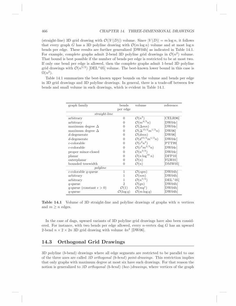
(straight-line) 3D grid drawing with O(|V (D)|) volume. Since |V (D)| = m log n, it followsthat every graph G has a 3D polyline drawing with O(m log n) volume and at most log nbends per edge. These results are further generalized [DW04b] as indicated in Table 14.1.For example, complete graphs admit 2-bend 3D polyline grid drawings in O(n2) volume.That bound is best possible if the number of bends per edge is restricted to be at most two.If only one bend per edge is allowed, then the complete graphs admit 1-bend 3D polylinegrid drawings with O(n5/2) [DEL+05] volume. The best-known lower bound in this case isΩ(n2).

Table 14.1 summarizes the best-known upper bounds on the volume and bends per edgein 3D grid drawings and 3D polyline drawings. In general, there is a trade-off between fewbends and small volume in such drawings, which is evident in Table 14.1.

graph family bends volume referenceper edge

straight-linearbitrary 0 O(n3) [CELR96]

arbitrary 0 O(m4/3n) [DW04c]maximum degree ∆ 0 O(∆mn) [DW04c]

maximum degree ∆ 0 O(∆15/2m1/2n) [DW06]d-degenerate 0 O(dmn) [DW06]

d-degenerate 0 O(d15/2m1/2n) [DW04c]c-colorable 0 O(c2n2) [PTT99]

c-colorable 0 O(c6m2/3n) [DW04c]

proper minor-closed 0 O(n3/2) [DW04c]planar 0 O(n log16 n) [DFP10]outerplanar 0 O(n) [FLW01]bounded treewidth 0 O(n) [DMW05]

polylinec-colorable q-queue 1 O(cqm) [DW04b]arbitrary 1 O(nm) [DW04b]

arbitrary 1 O(n5/2) [DEL+05]q-queue 2 O(qn) [DW04b]q-queue (constant ǫ > 0) O(1) O(mqǫ) [DW04b]q-queue O(log q) O(m log q) [DW04b]

Table 14.1 Volume of 3D straight-line and polyline drawings of graphs with n verticesand m ≥ n edges.

In the case of dags, upward variants of 3D polyline grid drawings have also been consid-ered. For instance, with two bends per edge allowed, every n-vertex dag G has an upward2-bend n× 2× 2n 3D grid drawing with volume 4n2 [DW06].

14.3 Orthogonal Grid Drawings

3D polyline (b-bend) drawings where all edge segments are restricted to be parallel to oneof the three axes are called 3D orthogonal (b-bend) point-drawings . This restriction impliesthat only graphs with maximum degree at most six have such drawings. For that reason thenotion is generalized to 3D orthogonal (b-bend) (box -)drawings, where vertices of the graph

14.3. ORTHOGONAL GRID DRAWINGS 467

are represented by pairwise non-intersecting boxes. A box is a rectanguloid with all of itscorners at grid points. A 3D orthogonal (b-bend) (box)-drawing where all boxes degenerateto cubes, line-segments, or points is called, respectively, a 3D orthogonal (b-bend) cube-,line-, or point-drawing.

The 3D orthogonal drawings have very good angular resolution, which makes them suit-able for numerous applications. Minimum edge separation and minimum vertex separationare also guaranteed in such drawings. Notice that neither good angular resolution nor goodedge separation is a feature of 3D (straight-line) grid drawings. The main quality measuresfor 3D orthogonal drawings are the volume and the number of bends (per edge). Othercriteria of importance include the length of the edges, and, in the case of 3D orthogonalbox-drawings, the size and the shape of the boxes. While the focus of this section is orthog-onal drawings in 3D, degree-4 graphs admit 3D polyline drawings with angular resolutioneven better than 90 degrees. Study of such drawings with small number of bends and goodvolume bounds has recently been initiated by Eppstein et al. [ELMN11].

It is NP-hard to optimize most of these aesthetic criteria for 3D orthogonal drawings. Us-ing straightforward extensions of known two-dimensional hardness results, Eades et al. [ESW96]showed that it is NP-hard to find a 3D orthogonal point-drawing of a graph that minimizesany one of the following aesthetic criteria: the volume, the number of bends per edge, thetotal number of bends, and the total edge length.

Not surprisingly, the 3D orthogonal point-drawings were the first to be studied; we con-sider them in the next section, followed by a review of 3D orthogonal box-drawings inSection 14.3.2.

14.3.1 Point-Drawings

In a 3D orthogonal point-drawing a vertex can have at most six neighbors. Thus only graphsof degree at most six may admit such drawings. In fact a graph has a 3D orthogonal point-drawing if and only if its maximum degree is at most six. This result will be discussedshortly (Theorem 14.8 below). The drawings used in establishing this result have manybends. This is unavoidable, since every 3D orthogonal point-drawing of the triangle (thatis, K3) obviously has at least one bend. Moreover, to draw an edge between any pair ofvertices not on the same grid line, at least one bend is required, and to draw and edgebetween a pair not on the same grid plane, at least two bends are required. This shedslight on the fact that no nontrivial class of graphs (excluding trees) is known to admit 3Dorthogonal point-drawings with zero bends. Less obvious is the well-known result that any3D orthogonal point-drawing of a multi-graph comprising of two vertices and six edges hasan edge with at least three bends. For simple graphs, K5 requires an edge with at least twobends [Woo03a]. This provides the best-known lower bound on the number of bends peredge for 3D orthogonal point-drawings of degree-6 graphs.

Volume Θ(n3/2):

One of the earliest results concerning 3D orthogonal point-drawings is due to Kolmogorovand Barzdin [KB67] and established a lower bound of Ω(n3/2) for the volume of degree-6graphs. This lower bound was matched with an upper bound by Eades et al. [ESW96] toestablish the following theorem.

Theorem 14.8 [ESW96, KB67] Every n-vertex degree-6 graph has a 3D orthogonal point-drawing in O(n3/2) volume, and that bound is best possible for some degree-6 graphs.


Figure 14.5 3D orthogonal 2-bend point-drawing of K5 (in coplanar model).

To obtain the upper bound, Eades et al. [ESW96] developed an O(n)-time algorithm1

that produces a 3D orthogonal point-drawing for a degree-6 graph G. Their algorithm isa modification of the method developed by Kolmogorov and Barzdin [KB67] for a similarproblem. The algorithm places all the vertices of G on an O(n) × O(n) grid in the Z = 0plane and draws each edge with at most sixteen bends. This model of drawing where allthe vertices intersect one grid plane is known as the coplanar model. Figure 14.5 illustratesa 2-bend orthogonal point-drawing of K5 in the coplanar model.

2 and 3 Bends:

Theorem 14.8 states that for the point-drawings, the optimal volume for degree-6 graphsis known (at least asymptotically). The situation is different for the number of bends peredge. As noted above two bends per edge may be necessary. The best-known upper boundis three. This result was first proved by Eades et al. [ESW00].

Theorem 14.9 [ESW00] Every degree-6 graph has a 3D 3-bend orthogonal point-drawing.

We now overview the most commonly used approach for producing 3D orthogonal point-drawings. The approach was first taken by Eades et al. [ESW00] in their 3-bend algorithmthat establishes Theorem 14.9.

A cycle cover of a graph G, also called a 2-factor, is a 2-regular spanning subgraph of G,that is, a spanning subgraph that consists of cycles. If the graph is directed, then the cyclesin the cover are required to be directed as well. Eades et al. [ESW00] gave an algorithmicproof that the edges of every degree-6 graph G can be oriented in such a way that G is asubgraph of some directed graph G′ (possibly with loops) such that the edges of G′ can becolored with three colors each of which induces a directed cycle cover of G′. The proof canbe viewed as a repeated application of the classical result of Petersen that every regulargraph of even degree has a 2-factor. The cycle covers can be computed in O(n) time forn-vertex graphs.

Having this in mind, most algorithms for producing 3D orthogonal point-drawings startoff with the decomposition of G′ into three cycle covers, denoted, say, by Cred, Cblue, andCgreen. In the second step vertices of G′ are positioned on the 3D grid in some way thatmakes drawing the red cycles easy. For example, in the coplanar model, vertices can beplaced in the Z = 0 plane and all red edges can be drawn in that plane. The remaining

1The running time in the conference paper is O(n3/2). This was later reduced in [ESW00].


edges Cblue and Cgreen are then routed above and below the Z = 0 plane, respectively. Ingeneral, the third step involves finding drawings for the edges in Cblue and Cgreen.The 3-bend algorithm of Eades et al. [ESW00] positions each vertex vi of G

′ at (3i, 3i, 3i)for some arbitrary vertex ordering (v1, v2, . . . , vn) of V (G′). This model of 3D orthogonalpoint-drawings, where vertices are place along the 3D diagonal of a cube, is called thediagonal model. The resulting drawings have volume at most 8n3 after all the grid planesnot containing a vertex or a bend are deleted. Wood [Woo04] modifies the 3-bend algorithmof Eades et al. [ESW00] to produce 3-bend drawings in the diagonal model with n3 + o(n3)volume, which is to date the best volume bound on 3D orthogonal 3-bend drawings. Toachieve this, Wood places each vertex vi of G′ at (i, i, i) in a particular vertex ordering(v1, v2, . . . , vn) stemming from book embeddings. For more on book embeddings, refer tothe next section on graph thickness. While the algorithm of Eades et al. runs in O(n) time,the algorithm of Wood runs in O(n5/2) time due to the book embedding computation. Thediagonal model was also used in the incremental algorithm of Papakostas and Tollis [PT99].Their algorithm, which runs in O(n) time, supports on-line insertion of vertices in constanttime. The resulting 3D orthogonal 3-bends point-drawings have volume at most 4.63n3.

The upper bound from Theorem 14.9 and the lower bound of two on the number of bendsper edge leave the following open problem.

Open Problem 14.4 [ESW00] Does every degree-6 graph have a 3D 2-bend orthogonalpoint-drawing?

This problem is considered to be the most important open problem concerning 3D orthog-onal point-drawings. The answer to the question remains unknown even when attentionis restricted to more specific classes of graphs, including degree-6 planar graphs, degree-6series-parallel graphs, and degree-6 outerplanar graphs. It is easy to observe that everydegree-6 tree has a 3D orthogonal point-drawing with no bends.A natural candidate for answering Open Problem 14.4 in the negative was K7, as con-

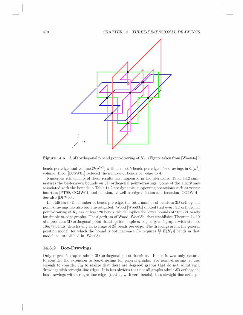
jectured in the conference version of [ESW00]. The counterexample to that conjecture wasdiscovered by Wood [Woo03a]. His construction is illustrated in Figures 14.6 and 14.7(courtesy of David R. Wood). Moreover, Wood exhibited 3D 2-bend point-drawings forother small multipartite 6-regular graphs: K6,6, K3,3,3 and K2,2,2,2.For degree-5 graphs, Wood [Woo03b] answered Open Problem 14.4 in the affirmative.

Theorem 14.10 [Woo03b] Every degree-5 graph has a 3D 2-bend orthogonal point-drawing.

The O(n2)-time algorithm of Wood that establishes this result produces 3D orthogonalpoint-drawings of degree-6 graphs in the so-called general position model, where no pair ofvertices belongs to the same grid plane. (Note, for example, that a drawing in the diagonalmodel is also in the general position model.) In the case of degree-5 graphs, the algorithmoutputs 2-bend drawings in the general position model. While this model allows for 2-benddrawings for degree-5 graphs, the same is not the case for degree-6 graphs. In particular,Wood [Woo03a] constructed an infinite family of degree-6 graphs that have an edge with atleast 3 bends in every 3D orthogonal point-drawing in the general position model.

Tradeoffs and more bounds:

Tradeoff issues between the maximum number of bends per edge and the volume of 3Dorthogonal point-drawings were first studied by Eades et al. [ESW00]. They began with analgorithm to draw a degree-6 graph in the coplanar model with O(n3/2) volume and at most7 bends per edge. By successive refinements of this algorithm, they obtained 3D orthogonalpoint-drawings of degree-6 graphs with the following bounds: volume O(n2) with at most 6


X

Y

Z

Figure 14.6 A 3D orthogonal 2-bend point-drawing ofK7. (Figure taken from [Woo03a].)

bends per edge, and volume O(n5/2) with at most 5 bends per edge. For drawings in O(n2)volume, Biedl [BJSW01] reduced the number of bends per edge to 4.

Numerous refinements of these results have appeared in the literature. Table 14.2 sum-marizes the best-known bounds on 3D orthogonal point-drawings. Some of the algorithmsassociated with the bounds in Table 14.2 are dynamic, supporting operations such as vertexinsertion [PT99, CGJW01] and deletion, as well as edge deletion and insertion [CGJW01].See also [DPV00].

In addition to the number of bends per edge, the total number of bends in 3D orthogonalpoint-drawings has also been investigated. Wood [Woo03a] showed that every 3D orthogonalpoint-drawing of K7 has at least 20 bends, which implies the lower bounds of 20m/21 bendsfor simple m-edge graphs. The algorithm of Wood [Woo03b] that establishes Theorem 14.10also produces 3D orthogonal point-drawings for simple m-edge degree-6 graphs with at most16m/7 bends, thus having an average of 2 2

7 bends per edge. The drawings are in the generalposition model, for which the bound is optimal since K7 requires 16

7 |E(K7)| bends in thatmodel, as established in [Woo03a].

14.3.2 Box-Drawings

Only degree-6 graphs admit 3D orthogonal point-drawings. Hence it was only naturalto consider the extension to box-drawings for general graphs. For point-drawings, it wasenough to consider K3 to realize that there are degree-6 graphs that do not admit suchdrawings with straight-line edges. It is less obvious that not all graphs admit 3D orthogonalbox-drawings with straight-line edges (that is, with zero bends). In a straight-line orthogo-


X

Y

Z

Figure 14.7 Breakaway view of the 3D orthogonal 2-bend point-drawing of K7. (Figuretaken from [Woo03a].)

graph family max. (avg.) bends volume referenceper edge

multigraph 7 Θ(n3/2) [ESW00]

multigraph (dynamic) 14 Θ(n3/2) [BJSW01]multigraph 4 O(n2) [BJSW01]multigraph (dynamic) 5 O(n2) [CGJW01]multigraph ∆ ≤ 4 3 O(n2) [ESW00]simple 4 (2 2

7) 2.13n3 [Woo03b]

multigraph (dynamic) 3 4.63n3 [PT99]multigraph 3 n3 + o(n3) [Woo04]simple ∆ ≤ 5 2 n3 [Woo03b]

Table 14.2 The volume and the number of bends per edge in 3D orthogonal point-drawings of n-vertex graphs with maximum degree ∆ ≤ 6.

nal box-drawing of a graph G, each edge is a line segment parallel to one of the three axes.This defines an associated coloring of the edges with three colors, where a subgraph of Ginduced by each color class has a visibility representation by rectangles. (Refer to the lastsection, page 478, for the definition of a visibility representation.) Bose et al. [BEF+98]proved that Kn does not have such a representation for n ≥ 56.


Ramsey theory implies that for every constant c ∈ N there is a constant r(c) (the Ramseynumber) such that every edge 3-coloring of the complete graph Kn with n ≥ r(c) containsa monochromatic subgraph isomorphic to Kc. With c = 56, that establishes the fact thatKr(56) does not have a straight-line 3D orthogonal box-drawing. This argument (in threeand higher dimensions) was first pointed out by Biedl et al. [BSWW99]. The constantr(56), stemming from Ramsey theory, is a truly big number. Fekete and Meijer [FM99]significantly improved that upper bound to K184. Their proof uses the fact that K56 doesnot have a 3D rectangle visibility representation. The largest complete graph known toadmit a straight-line 3D orthogonal box-drawing is K56 [FM99].

The above discussion highlights that not all graphs have 3D orthogonal box-drawingswith zero bends. Indeed, it is easy to observe that every n-vertex m-edge graph G hasan orthogonal (line)-drawing with one bend per edge: simply represent each vertex vi,1 ≤ i ≤ n, of G by a line-segment with endpoints (i, i, 1) and (i, i,m), and then draweach edge in distinct Z = j planes, 1 ≤ j ≤ m, using one bend. The resulting drawing hasO(n2m) volume. Better volume bounds are possible for 3D orthogonal 1-bend box-drawings.Biedl et al. [BSWW99] showed that in the previous construction with the segments havingendpoints at (i, i, 1) and (i, i, n), it is possible to draw all the edges of Kn in Z = j,1 ≤ j ≤ m, using one bend per edge. They suggested a relationship between assigningedges to the planes in this type of drawing and assigning edges to the pages of a bookembedding. This relationship was later explored by Wood [Woo01], resulting in improvedvolume bounds for 1-bend box-drawings of m-edge graphs. In particular, he proved thatevery graph has a 3D orthogonal 1-bend box-drawing in O(n3/2m) volume.

A lower bound of Ω(n5/2) for the volume of 3D orthogonal box-drawings of n-vertexgraphs (regardless of the number of bends) was established by Biedl et al. [BSWW99].They developed an O(m)-time algorithm that constructs drawings matching that volumebound and using at most 3 bends per edge, thus establishing that all n-vertex graphs have3D orthogonal 3-bend box-drawings in Θ(n5/2) volume. Closing the gap between the O(n3)upper bound and the Ω(n5/2) lower bound for 3D orthogonal 1-bend box-drawings of Kn

remains an interesting open problem.The lower bound of Biedl et al. [BSWW99] was established using the complete graph Kn.

The proof relies critically on the fact that between any two disjoint vertex sets of size Ω(n)in Kn, there are Θ(n2) edges. To generalize this lower bound to sparse graphs and to be ableto express it in terms of the number of edges, Biedl et al. [BTW06] exhibited graphs suchthat between any two disjoint vertex sets of size Ω(n) there are Θ(m) edges. That allowedthem to extend the arguments of [BSWW99] to establish the lower bound of Ω(m

√n) on

the volume of 3D orthogonal box-drawings of m-edge n-vertex graphs. They developedan O(m2/

√n)-time algorithm that constructs drawings matching that volume bound and

using at most 4 bends per edge, thus establishing that all graphs have 3D orthogonal 4-bend box-drawings in Θ(m

√n) volume. It is unknown whether all m-edge graphs admit

3D orthogonal box-drawings with such volume and at most 3 bends per edge, as is the casefor Kn.

The discussion above pertains to drawings where the volume and the number of bendsper edge are the only concerns. The shapes and the sizes of boxes used to represent verticesare unrestricted. However, for box-drawings the size and the shape of a vertex with respectto its degree are also important aesthetic criteria. For a vertex v in a 3D orthogonal box-drawing the surface of v is the number of grid lines intersecting the box-representing v timestwo. The surface of v indicates the number of grid lines available for drawing edges incidentto v. In point-drawings, for example, the surface of each vertex is six. Generally, in any3D orthogonal box-drawing, the surface of each vertex v is at least the degree of v. Ideally,the surface of v should also not be much bigger than the degree of v. Biedl et al. [BTW06]

14.4. THICKNESS 473

defined a 3D orthogonal box-drawing of a graph G to be degree-restricted if there existssome constant α ≥ 1 such that for every vertex v in G, surface(v) ≤ α·degree(v).

Degree-restricted drawings do not, however, impose any aesthetic restriction on the shapeof the boxes used to represent vertices. The aspect ratio of a vertex in a 3D orthogonalbox-drawing is the ratio of the length (measured in the number of grid points) of the longestside of the box representing that vertex to the shortest side of that box. 3D orthogonalbox-drawings have a bounded vertex-aspect ratio if there exists a constant r such that allvertices have aspect ratios at most r. Note that r ≥ 1, and for the case of 3D orthogonalpoint-drawings and cube-drawings, it is one. Also note that degree-restricted drawings mayhave unbounded vertex-aspect ratio; consider, for example, a drawing in which each vertexis represented by a segment with length equal to its degree.

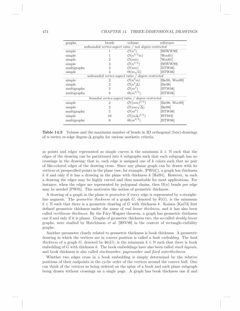
The discussion at the beginning of this subsection pertains to 3D orthogonal box-drawingswith (possibly) unbounded vertex-aspect ratios and with no degree-restrictions. The best-known upper bounds on the volume and the number of bends per edge in such unrestricted3D orthogonal box-drawings are summarized in the top part of Table 14.3. The upperbounds can be compared to the best-known lower bound on the volume of such drawingswhich, as discussed above, is Ω(m

√n) regardless of the number of bends [BTW06]. The

table exhibits the tradeoff between the number of bends per edge and the volume of suchdrawings.

Biedl et al. [BTW06] derived lower bounds for the volume of 3D orthogonal box-drawingsthat are required to be degree-restricted and/or have bounded vertex-aspect ratio. Inparticular, they proved an Ω(m3/2/α) lower bound on the volume of 3D orthogonal box-drawings that are degree-restricted for some α ≥ 1, as well as an Ω(m3/2/

√r) lower bound

on the volume of 3D orthogonal box-drawings for which each vertex has aspect ratio at mostr. For bounded α and bounded r, both bounds become Ω(m3/2). The discussion pertainingto the proof technique of Biedl et al. [BTW06] used to derive the Ω(m

√n) volume bound

for unrestricted drawings applies to these two lower bounds as well.

Biedl et al. [BTW06] also developed an algorithm that constructs the corresponding 3Dorthogonal box-drawings matching the volume lower-bound and using at most 6 bendsper edge, thus establishing that all m-edge graphs have 3D orthogonal 6-bend box-drawingswith volume Θ(m3/2) such that the drawings are degree-restricted and have bounded aspectratio.

The best-known upper bounds on the volume and the number of bends per edge in degree-restricted 3D orthogonal box-drawings are summarized in the middle part of Table 14.3,while drawings that are both degree-restricted and have bounded vertex-aspect ratio areaddressed at the bottom of the table. These upper bounds on the volume can be comparedto the best-known lower bound of Ω(m3/2).

The table reveals that no further asymptotic improvements are possible for the volume ofdrawings in all three aesthetic models discussed. There is room for improvement, however,with regard to the number of bends per edge, as suggested by some of the open problemsmentioned in this subsection.

14.4 Thickness

Thickness is a classical graph parameter that has been studied since the early 1960s. Itwas first defined by Tutte [Tut63]. The thickness of a graph G, denoted by θ(G), is theminimum k ∈ N such that the edge set of G can be partitioned into k planar subgraphs.

For ease of exposition in this section, we express the concept of thickness in terms ofdrawings in the plane. The thickness of a drawing in the plane with vertices represented


graphs bends volume referenceunbounded vertex-aspect ratio / not degree-restricted

simple 1 O(n3) [BSWW99]

simple 1 O(n3/2m) [Woo01]simple 2 O(nm) [Woo01]

simple 3 O(n5/2) [BSWW99]multigraphs 3 O(nm) [BTW06]simple 4 Θ(m

√n) [BTW06]

unbounded vertex-aspect ratio / degree-restrictedsimple 2 O(n2m) [Bie98, Woo99]simple 2 O(n2∆) [Bie98]multigraphs 5 O(m2) [BTW06]

multigraphs 6 Θ(m3/2) [BTW06]

bounded vertex-aspect ratio / degree-restricted

simple 2 O((nm)3/2) [Bie98, Woo99]

simple 2 O(nm√∆) [Bie98]

multigraphs 5 O(m2) [BTW06]

simple 10 O((n∆)3/2) [HTS83]

multigraphs 6 Θ(m3/2) [BTW06]

Table 14.3 Volume and the maximum number of bends in 3D orthogonal (box)-drawingsof n-vertex m-edge degree-∆ graphs for various aesthetic criteria.

as points and edges represented as simple curves is the minimum k ∈ N such that theedges of the drawing can be partitioned into k subgraphs such that each subgraph has nocrossings in the drawing; that is, each edge is assigned one of k colors such that no pairof like-colored edges of the drawing cross. Since any planar graph can be drawn with itsvertices at prespecified points in the plane (see, for example, [PW01]), a graph has thicknessk if and only if it has a drawing in the plane with thickness k [Hal91]. However, in sucha drawing the edges may be highly curved and thus unsuitable for most applications. Forinstance, when the edges are represented by polygonal chains, then Ω(n) bends per edgemay be needed [PW01]. This motivates the notion of geometric thickness.

A drawing of a graph in the plane is geometric if every edge is represented by a straight-line segment. The geometric thickness of a graph G, denoted by θ(G), is the minimumk ∈ N such that there is a geometric drawing of G with thickness k. Kainen [Kai73] firstdefined geometric thickness under the name of real linear thickness, and it has also beencalled rectilinear thickness. By the Fary-Wagner theorem, a graph has geometric thicknessone if and only if it is planar. Graphs of geometric thickness two, the so-called doubly lineargraphs, were studied by Hutchinson et al. [HSV99] in the context of rectangle-visibilitygraphs.

Another parameter closely related to geometric thickness is book thickness. A geometricdrawing in which the vertices are in convex position is called a book embedding. The bookthickness of a graph G, denoted by bt(G), is the minimum k ∈ N such that there is bookembedding of G with thickness k. The book embeddings have also been called stack layouts,and book thickness is also called stacknumber, pagenumber and fixed outerthickness.

Whether two edges cross in a book embedding is simply determined by the relativepositions of their endpoints in the cyclic order of the vertices around the convex hull. Onecan think of the vertices as being ordered on the spine of a book and each plane subgraphbeing drawn without crossings on a single page. A graph has book thickness one if and

14.4. THICKNESS 475

only if it is outerplanar [BK79]. Bernhart and Kainen [BK79] proved that a graph has bookthickness at most two if and only if it is a subgraph of a Hamiltonian planar graph. Unlikethickness, being able to partition the edge set of a graph G into k outerplanar subgraphsdoes not imply that G has book thickness at most k. For example, the edge set of K5 canbe partitioned into two cycles, yet K5 has book thickness more than two, since it is not asubgraph of a Hamiltonian planar graph. The situation is similar for geometric thicknessas will soon become clear.

Book embeddings, first defined by Ollmann [Oll73], are ubiquitous structures with avariety of applications; see [DW04a] for a survey with over 50 references. These applicationsinclude sorting permutations, fault-tolerant VLSI design, and compact graph encodingsas well as graph drawing. In general, drawings arising from the study of thickness haveapplications in graph visualization (where each plane subgraph is colored by a distinctcolor), and in multilayer VLSI (where each plane subgraph corresponds to a set of wiresthat can be routed without crossings in a single layer).

First we consider the relationship between the three thickness parameters. By definition,for every graph G

θ(G) ≤ θ(G) ≤ bt(G). (14.1)

These inequalities have been shown to be strict for certain graphs [DEH00]. In the otherdirection, no such relationship is possible for any bounding function. Eppstein [Epp01]proved that geometric thickness is not bounded by any function of book thickness. In par-ticular, the graph obtained by subdividing each edge of Kn once has geometric thickness atmost two. On the other hand, a Ramsey-theoretic argument shows that the book thicknessof that graph is not bounded by any constant.

Using a more elaborate Ramsey-theoretic argument applied to graphs formed by start-ing with n points and adding a new point adjacent to each triple of the n points, Epp-stein [Epp04a] proved that geometric thickness is not bounded by any function of thickness.In particular, for every t there exists a graph with thickness three and geometric thicknessat least t. This leaves an interesting open problem.

Open Problem 14.5 [Epp04a] Do graphs with thickness two have bounded geometric thick-ness?

Complete graphs: The thickness of the complete graph Kn was intensely studied in the1960s and 1970s. Results by a number of authors [AG76, Bei67, BH65, May72] togetherprove that θ(Kn) = ⌈(n+ 2)/6⌉, unless n = 9 or 10, in which case θ(K9) = θ(K10) = 3.

Bernhart and Kainen [BK79] proved that bt(Kn) = ⌈n/2⌉. In fact, they proved thatevery convex drawing of Kn can be partitioned into ⌈n/2⌉ plane spanning paths.

Bose et al. [BHRCW06] proved that every geometric drawing of Kn has thickness at mostn −

√

n/12. It is unknown whether every geometric drawing of Kn has thickness at most(1− ǫ)n. Dillencourt et al. [DEH00] studied the geometric thickness of Kn, and proved that

⌈(n/5.646) + 0.342⌉ ≤ θ(Kn) ≤ ⌈n/4⌉ . (14.2)

Their upper bound construction generalizes to show that for any n, θ(Kn) ≤ ⌈n/4⌉.What is θ(Kn)? It seems likely that the answer is closer to ⌈n/4⌉ rather than to the abovelower bound.

Maximum degree: Next, we consider the relationships among the three thickness parametersand the maximum degree. Recall that, a graph with maximum degree ∆ is called a degree-∆ graph. Wessel [Wes84] and Halton [Hal91] proved independently that the thickness of a


degree-∆ graph is at most ⌈∆/2⌉. The proof is based on the classical result of Petersen thatevery regular graph of even degree has a 2-factor, that is, a set of vertex disjoint cycles thattogether cover all the vertices. The theorem implies that the edges of a ∆-regular graphfor even ∆ can be partitioned into ∆/2 sets of vertex disjoint cycles. Vertex disjoint cyclesare planar, and thus the upper bound follows by proving that every degree-∆ graph is asubgraph of some ∆-regular graph. Sykora et al. [SSV04] proved that this bound is tight.Malitz [Mal94b] proved that there exist ∆-regular n-vertex graphs with book thickness at

least Ω(√∆n1/2−1/∆). Thus, unlike thickness, book thickness is not bounded by any func-

tion of maximum degree. The proof is based on a probabilistic construction. Malitz [Mal94b]also derived an upper bound of O(

√m) ∈ O(

√∆n) for the book thickness, and thus the

geometric thickness, of m-edge graphs.Eppstein [Epp04a] asked whether bounded degree graphs have bounded geometric thick-

ness. Duncan et al. [DEK04] gave an affirmative answer for degree-4 graphs. By Petersen’stheorem, the edges of a degree-4 graph G can be partitioned into two sets each of which in-duces a subgraph comprised of vertex disjoint paths and cycles in G. Duncan et al. [DEK04]proved that two such subgraphs can be drawn simultaneously on some planar point set us-ing straight-line edges, thus proving that G has a geometric drawing with thickness at mosttwo. Moreover, they provided a linear-time algorithm to produce such thickness-2 geometricdrawings for degree-4 graphs. In the case of degree-3 graphs, the resulting drawings fit inthe n× n grid.

In a recent development, the above-mentioned question of Eppstein has been answeredin the negative. Barat et al. [BMWR3] have shown that bounded degree graphs may haveunbounded geometric thickness, even approaching the square root of the number of vertices.In particular, for all ∆ ≥ 9 there exists a ∆-regular n-vertex graph with geometric thicknessΩ(

√∆n1/2−4/∆−ǫ). The proof is non-constructive and based on counting arguments. The

authors have shown that there are more graphs with bounded degree than with boundedgeometric thickness. To count the number of n-vertex graphs of thickness k, they consideredthe number of order types of n points and all the ways of connecting the points in an ordertype into a geometric drawing of thickness k.

Open Problem 14.6 [BMWR3] Do degree-∆ graphs with ∆ ∈ 5, 6, 7, 8 have boundedgeometric thickness?

Proper minor-closed families: Blankenship and Oporowski [Bla03, BO01] proved that allproper minor-closed families have bounded book thickness and therefore, by Equation 14.1,bounded thickness and geometric thickness. Proper minor-closed families include, for ex-ample, planar graphs, bounded genus graphs, and bounded treewidth graphs. The proofdepends on Robertson and Seymour’s deep structural characterization of the graphs exclud-ing a fixed minor. As a result, the obtained bound on book thickness for graphs excludinga Kℓ-minor is a truly huge function of ℓ.A much better bound is known for the thickness of such families. Kostochka [Kos82] and

Thomason [Tho84] proved independently that graphs excluding a Kℓ-minor have thicknessat most O(ℓ log ℓ). Better bounds on book thickness (and thus geometric thickness) are alsoknown for many minor-closed families. The question of book thickness of planar graphs wassettled by Yannakakis [Yan86] in 1986: he proved that the book thickness of planar graphsis at most four and that there are planar graphs with book thickness matching that bound.There is some dispute over this lower bound. The construction is given in the conferenceversion of the paper only [Yan86], where the proof is far from complete.

Endo [End97] determined that the book thickness of toroidal graphs, that is, graphs withgenus one, is at most seven. Malitz [Mal94a] proved by a probabilistic argument that thebook thickness of graphs with genus γ is at most O(

√γ).

14.5. OTHER (NON-GRID) 3D DRAWING CONVENTIONS 477

Exact bounds are known for all three thickness parameters in relation to treewidth. Inparticular, for graphs of treewidth k the maximum thickness and the maximum geometricthickness both equal ⌈k/2⌉ [DW05]. This says that the lower bound for thickness can bematched by an upper bound, even in the more restrictive geometric setting. For graphs oftreewidth k, the maximum book thickness equals k if k ≤ 2 and equals k+1 if k ≥ 3. Whilethe lower bounds are proved in [DW05], the upper bounds on book thickness are due toGanley and Heath [GH01].

Computational complexity: The graphs with book thickness one are precisely the outer-planar graphs [BK79], and thus can be recognized in linear time. The graphs with bookthickness two are characterized as the subgraphs of planar Hamiltonian graphs [BK79],which implies that it is NP-complete to test if bt(G) ≤ 2 [Wig82]. In fact, even deter-mining thickness of a given book embedding is hard. Specifically, a book embedding withk pairwise crossing edges has thickness at least k, since each edge must receive a distinctcolor. However, the converse is not true. There exist book embeddings with no (k + 1)pairwise crossing edges for graphs that have thickness at least Ω(k log k) [KK97]. Moreover,it is NP-complete to test if a given book embedding of a graph has thickness k [GJMP80].

Testing whether a graph has thickness k is NP-hard [Man83] even for k = 2. Eppstein[Epp04b] considered the problem of testing if a given geometric drawing has thickness k. Fork = 2 the problem can be solved in polynomial time but becomes NP-complete for k ≥ 3.Dillencourt et al. [DEH00] asked what the complexity is for determining the geometricthickness of a given graph.

Open Problem 14.7 [DEH00] Is it NP-hard to test if the geometric thickness of a graphis k?

We close this section with an open problem that relates book thickness and 3D griddrawings.

Open Problem 14.8 [DW04b] Do all bipartite graphs that have book thickness three havebounded track-number?

By studying book thickness of graph subdivisions Dujmovic and Wood [DW04b] provedthat an affirmative answer to this question would imply an affirmative answer to OpenProblems 14.1, 14.2, and 14.3. More generally, it would imply that the queue-number isbounded by book-thickness, which is a long standing open problem [HLR92]. Since allproper minor-closed graph families have bounded book thickness [BO01], an affirmativeanswer to this question would further imply that all proper minor-closed graph familieshave linear volume 3D grid drawings.

14.5 Other (Non-Grid) 3D Drawing Conventions

3D crossing-free straight-line drawings with real coordinates: Three dimensional straight-linecrossing-free graph drawings in which the vertices are allowed real coordinates have also beenstudied. Naturally, having a less restrictive model allows for drawings with better bounds,for example better volume bounds, in comparison to the grid model. One disadvantage tousing real coordinates, however, becomes evident when a drawing is to be displayed, ona computer screen for example. Then the real vertex coordinates must be converted intointeger coordinates. There are no guarantees that rounding off will maintain the correctnessof the embedding.


As in the grid model, the main criterion for measuring the quality of a drawing is its vol-ume. To make a discussion about volume meaningful, that is, to disallow arbitrary scaling,the vertices are required to lie at least unit distance apart. As noted in the introduction,a classical result of Steintz states that the triconnected planar graphs are exactly the 1-skeletons of convex polyhedra in 3D, that is, they admit 3D convex drawings. This maybe considered as one of the first results in the real coordinates model. The construction,however, seems to require exponential volume in the number of vertices of a graph. Thesame is true for the number of bits needed to represent the coordinates of the vertices. Thisoutlook has been greatly improved by Chrobak et al. [CGT96]. The technique they used toderive their results falls under the category of so-called force directed methods.

Force directed methods model the graph as a physical system. For example, edges can bemodeled as springs and vertices as charged particles that repel each other. A configurationwhere the sum of the forces on each particle is zero, that is, a local minimum of the system,gives a straight-line drawing of the graph. The famous barycenter method developed byTutte [Tut60] is an example of the force directed approach. Specifically, the barycentermethod takes a 3-connected plane graph G and fixes the vertices of the outer face in aconvex position in the plane. The remaining vertices of G are then added one by one at thebarycenter of their neighbors. The resulting system of linear equations gives coordinates forthe internal vertices, and results in a 3D drawing of G where all internal faces are convex.This method can be extended to 3D.

As noted above, the best-known bounds are due to Chrobak et al. [CGT96]. They de-veloped a force-directed algorithm that, given an n-vertex triconnected planar graph G,outputs a 3D drawing of G with O(n) volume. Moreover, the vertex coordinates in thedrawing can be represented by O(n log n)-bit rational numbers. The algorithm runs inO(M(n1/2)) time, where M(n) is the time needed to multiply two n × n matrices. Theyalso showed that if the minimum angle between two edges incident to the same vertex isrequired to be some fixed function of the maximum degree, then there are bounded-degreetriconnected planar graphs that require 2Ω(n) volume in any 3D convex drawing.

In other results in the real coordinate model, Garg et al. [GTV96] proved that all graphswith bounded chromatic number can be drawn in O(n3/2) volume with constant aspectratio and using O(log n)-bit rational numbers for vertex coordinates. If the number of bitsis increased to O(n log n), they showed that all graphs have 3D straight-line crossing-freedrawings in O(n) volume. Their algorithms run in O(n) time provided that the graphcoloring is given as a part of the input.

Simulated annealing techniques for generating 3D straight-line drawings of general graphshave also been considered [CT96].

3D graph representations: In a graph representation, vertices are depicted as some set ofobjects and edges indicate a relationship between the objects. In the case of visibilityrepresentations, for example, there is an edge between two vertices in the graph if and onlyif there is a line-segment that joins the objects representing the vertices and that does notintersect any other object, that is, if the two objects are (mutually) visible. Typically,these line-segments may be required to align with an axis. In two dimensions, popularvisibility representations studied are bar - and rectangle visibility . Both models are relatedto orthogonal drawings in the plane. Only thickness-2 graphs have such two-dimensionalvisibility representations, which motivates the study of 3D counterparts.

The concept generalizes naturally to three dimensions. The vertices may be disjoint2D objects parallel to the XY-plane, and the edges may be line-segments parallel to Z-axisconnecting pairs of visible objects. It is easy to see that all graphs have such a representationif the objects may be arbitrary non-convex polygons. Attention has therefore been restricted


to convex polygons. For instance, K7 has a representation with unit squares and K8 doesnot, and every graph has a representation with unit disks. Bose et al. [BEF+98] provedthat Kn has a representation with arbitrary rectangles for n ≤ 22, while for n ≥ 56 itdoes not. They also showed that all planar graphs and all complete bipartite graphs have arepresentation with arbitrary rectangles, but that the family of representable graphs is notclosed under graph minors.

Alt et al. [AGW98] considered representations with arbitrary convex polygons and showedthat there is no convex polygon P that would allow every complete graph to have a visibility

representation by shifted copies of P . In particular, for n > 22k

, Kn cannot be representedby a convex k-gon. This bound has been improved by Stola [Sto04], who proved thatthe maximum size of a complete graph with a visibility representation by copies of regu-lar k-gon is between k + 1 and 26k. Visibility representations with boxes have also beenconsidered [FM99].

Kotlov et al. [KLV97] discovered a relationship between graph representations by touchingspheres in 3D and the algebraic graph invariant µ introduced by Colin de Verdiere.

Surfaces and the theory of graph minors: The field of topological graph theory studiesgeometric realizations of graphs in 3-space and embeddings on surfaces. Embeddings ofgraphs on higher surfaces are a natural generalization of embeddings in the plane.The celebrated graph minors theorem of Robertson and Seymour [RS] implies that there

is a finite number of forbidden minors for graphs embeddable on any given fixed surface.The Kuratowski theorem identifies the forbidden minors for the plane. The projective planeis the only other surface for which all the forbidden minors (35 of them) are known. Mohar[Moh99] gave a linear-time algorithm that for any graph and any fixed surface S, eitherfinds an embedding of the given graph in S or identifies a subgraph homeomorphic to aforbidden minor for S.

The power of the graph minors theorem can be nicely illustrated by means of the following3D graph drawing problem. A graph is knotless if it has an embedding in 3D that doesnot contain a non-trivial knot, that is, if it has an embedding such that every cycle in theembedding bounds a disk. For example K7 is known not to have a knotless embedding.It is easy to observe that the class of all knotless graphs is minor-closed. One algorithmicconsequence of the graph minors theory is that there is a cubic time algorithm to testmembership of a graph in any proper minor-closed family. Thus, remarkably, there existsa cubic time algorithm to test if a graph is knotless. This problem was not even known tobe decidable before the advent of the graph minors theory. At present, however, no explicitalgorithm is known, let alone a polynomial-time one, as the theory only guarantees theexistence of such an algorithm.

A related concept is that of a linkless embedding. A graph is linkless if it has an embed-ding in 3D that does not contain a pair of linked cycles, that is, two cycles in the embeddingthat cannot be separated by a 2-sphere embedded in 3D. For example, K6 is known not tobe linkless. Unlike the case for knotless graphs, the full characterization of linkless graphsis known. In particular, a graph is linkless if and only if it does not contain as a minor oneof the six members of the Peterson family of graphs. A ∆Y -exchange in a graph replacesa triangle by a 3-star, while a Y∆-exchange replaces a 3-star by a triangle. The Petersonfamily is comprised of the six graphs that can be obtained from K6 by a sequence of ∆Y -and Y∆-exchanges. It is also known that a graph G is linkless if and only if its Colin deVerdiere invariant µ(G) is at most four. Whether knotless graphs are precisely those graphswhose Colin de Verdiere invariant is at most five is an interesting open problem.

Good viewpoints: In most visualization applications, a 3D drawing of a graph will eventuallybe displayed as an image on some kind of 2D medium, such as a computer screen or a sheet


of paper. This can be achieved by using projections. In computer graphics the mostcommonly used projections are the parallel and perspective projections. A 2D image, byits very nature, will necessarily contain less information than the original 3D drawing. It istherefore desirable to find viewpoints (the position and the direction the viewer is facing)that result in “nice” 2D images, that is, projections that preserve as much informationabout the 3D drawing as possible. Having an edge of the 3D drawing map to one point inthe projection is lossy in that context, as is having two vertices project to the same point.Bose et al. [BGRT99] developed an algorithm that, given a 3D straight-line drawing,

computes an arrangement of curves that describe all bad viewpoints for that drawing. Aviewpoint is bad if it maps three 3D points to the same point in the projection (verticescount as two points). Their algorithm runs in O(m4 logm+k) time, where m is the numberof edges of the graph and k may be O(m6) in the worst case.

The arrangement above distinguishes between bad and good viewpoints. Eades et al. stud-ied a model with a continuous measure of goodness for a viewpoint [EHW97]. In particularthe goodness of a viewpoint increases with distance from its nearest bad point. They alsoconsidered different definitions of bad points and developed an algorithm to compute thembased on techniques of Bose et al. [BGRT99].

3D symmetry: Connections between symmetry and aesthetics have long been recognized.Thus displaying automorphisms of a graph as symmetries in its drawing is a very desirablefeature. Drawing graphs symmetrically involves solving at least two problems. The first isto determine the symmetries (automorphisms) of a graph. The second problem is, giventhe graph automorphisms, to display as many of them as possible as geometric symmetriesof a drawing of the graph. Symmetries in 3D can be displayed by, for example, rotation,reflection, and inversion. For a detailed account on symmetric drawings, including 3Dsymmetric drawings, the reader is referred to Chapter 3.

Higher dimensions: One of the basic problems in discrete geometry is determining when agraph can be realized with prescribed edge lengths in R

d. An interesting graph invariantrelated to that concept is the dimension of a graph, introduced by Erdos et al. [EHT65].It is defined as the minimum d such that the graph has a drawing in R

d with straight-lineedges all of unit length (with possible crossings). They show, among other results, thatthe dimension of the complete graph Kn is n − 1 and that the dimension of the completebipartite graph is at most four.

A concept related to the dimensionality of a graph is that of realizability. A realizationof a graph is a straight-line “drawing” with vertices represented as points, where there is norestriction on how vertices and edges may intersect. A graph G is d-realizable if, given anyrealization of G in R

t, there exists a realization of G with the same edge-lengths in Rd. For

example, a path is 1-realizable since its vertices can be arranged on a line with any desirededge-lengths. A tree is also 1-realizable. On the other hand, the triangle is not 1-realizable,since it has a realization in R2 with unit distance edges but no such realization is possiblein R1. Connelly and Sloughter [BC07] proved that a graph is 1-realizable if and only if itis a forest. It is 2-realizable if and only if it has treewidth at most two, that is, if it is aseries-parallel graph. They showed that a graph is 3-realizable if and only if it does notcontain K5 or an octahedral graph as a minor.

A relationship between the connectivity of graphs and higher dimensional drawings hasbeen established [LLW88]. In particular, k-connected graphs were characterized in termsof particular convex drawings in R

k−1. A force directed method was used to derive theseresults.

Dujmovic et al. [DMS13] studied higher dimensional straight-line grid drawings (withpossible crossings). They showed that in every d-dimensional (d ≥ 4) straight-line grid


drawing of volume N of a graph with m ≥ (22 + 1)N edges, there are at least Ω(m2

N )crossings. They also showed that there are graphs for which this bound is tight.

Some other directions explored include the idea of producing 2D drawings by starting witha “nice” higher dimensional drawing of a graph and then projecting it to a plane. Higher-dimensional visibility representations with hyper-rectangles [CDH+96] have also been con-sidered.Applications and information visualization: This chapter was mainly focused on theory andfoundations of 3D Graph Drawing, that is, results with provable bounds on properties ondrawings and provable bounds on the running times of drawing algorithms. An importanttheme outside the scope of this chapter is that of development of software packages for 3Dgraph drawing (see, for example, [GT97, PV97]) as well as information visualization in 3D.Graph drawing in 3D relates to this area particularly because graphs model hierarchies andnetworks. Understanding large social and biological trees and networks requires the supportof visualization tools [BvLH+11, LLB+12, NJBJ09]. A substantial body of research litera-ture explores the possibility of combining 3D graphics and interactive animation technologywith an understanding of human perception for the purpose of conveying information, in-cluding graph models, to humans [XRP+12]. Classic work of Robertson et al. [RMC91]proposed to visualize organizational hierarchies with 3D animations of trees. Work onvisualization of graphs is found not only in the information visualization literature, butalso domain specific literature such as that of biology and bioinformatics. Important keywords include information visualization, human computer interaction, computer graphics,animation, human perception.


References

[AG76] V. B. Alekseev and V. S. Gonchakov. Thickness of arbitrary completegraphs. Mat. Sbornik, 101:212–230, 1976.

[AGW98] H. Alt, M. Godau, and S. Whitesides. Universal 3-dimensional visibilityrepresentations for graphs. Comput. Geom., 9:111–125, 1998.

[BC07] M. Belk and R. Connelly. Realizability of graphs. Discrete and Compu-tational Geometry, 37(2):125–137, 2007.

[BCMW04] P. Bose, J. Czyzowicz, P. Morin, and D. R. Wood. The maximum numberof edges in a three-dimensional grid-drawing. J. of Graph Algorithms andAppl., 8(1):21–26, 2004.

[BEF+98] P. Bose, H. Everett, S. Fekete, M. E. Houle, A. Lubiw, H. Meijer, K. Ro-manik, G. Rote, T. C. Shermer, S. Whitesides, and C. Zelle. A visibilityrepresentation for graphs in three dimensions. J. of Graph Algorithmsand Appl., 2(3):1–16, 1998.

[Bei67] L. W. Beineke. The decomposition of complete graphs into planar sub-graphs. In Graph Theory and Theoretical Physics, pages 139–154. 1967.

[BGRT99] P. Bose, F. Gomez, P. A. Ramos, and G. T. Toussaint. Drawing niceprojections of objects in space. J. of Visual Communic. and Image Rep-resentation, 10:155–172, 1999.

[BH65] L. W. Beineke and F. Harary. The thickness of the complete graph.Canad. J. Math., 17:850–859, 1965.

[BHRCW06] P. Bose, F. Hurtado, E. Rivera-Campo, and D. R. Wood. Partitions ofcomplete geometric graphs into plane trees. Computational Geometry:Theory and Applications, 34(2):116–125, 2006.

[Bie98] T. C. Biedl. Three approaches to 3D-orthogonal box-drawings. In Proc.6th Int. Symp. on Graph Drawing (GD’98), volume 1547 of LNCS, pages30–43. Springer, 1998.

[BJSW01] T. Biedl, J. R. Johansen, T. C. Shermer, and D. R. Wood. Orthogonaldrawings with few layers. In Proc. 9th Int. Symp. on Graph Drawing(GD’01), volume 2265 of LNCS, pages 297–311. Springer, 2001.

[BK79] F. Bernhart and P. C. Kainen. The book thickness of a graph. J. Combin.Theory Ser. B, 27(3):320–331, 1979.

[Bla03] Robin Blankenship. Book Embeddings of Graphs. PhD thesis, Dept. ofMathematics, Louisiana State University, U.S.A., 2003.

[BMWR3] J. Barat, J. Matousek, and D. R. Wood. Bounded-degree graphs havearbitrarily large geometric thickness. The Electronic Journal of Combi-natorics, 13, 2006, R3.

[BO01] R. Blankenship and B. Oporowski. Book embeddings of graphs andminor-closed classes. In Proc. 32nd Southeastern Int. Conf. on Com-binatorics, Graph Theory and Comp. Dept. of Math., Louisiana StateUniversity, 2001.

[BSWW99] T. C. Biedl, T. C. Shermer, S. Whitesides, and S. K. Wismath. Boundsfor orthogonal 3-D graph drawing. J. of Graph Algorithms and Appl.,3(4):63–79, 1999.

[BTW06] T. Biedl, T. Thiele, and D. R. Wood. Three-dimensional orthogonalgraph drawing with optimal volume. Algorithmica, 44(3):233–255, 2006.

REFERENCES 483

[BvLH+11] S. Bremm, T. von Landesberger, M. Hess, T. Schreck, P. Weil, andK. Hamacherk. Interactive visual comparison of multiple trees. In VisualAnalytics Science and Technology (VAST), 2011 IEEE Conference on,pages 31–40, 2011.

[CDH+96] F. Cobos, J. Dana, F. Hurtado, A. Marquez, and F. Mateos. On avisibility representation of graphs. In Proc. Int. Symp. on Graph Drawing(GD’95), volume 1027 of LNCS, pages 152–161. Springer, 1996.

[CELR96] R. F. Cohen, P. Eades, T. Lin, and F. Ruskey. Three-dimensional graphdrawing. Algorithmica, 17(2):199–208, 1996.

[CGJW01] M. Closson, S. Gartshore, J. Johansen, and S. K. Wismath. Fully dy-namic 3-dimensional orthogonal graph drawing. J. of Graph Algorithmsand Appl., 5(2):1–34, 2001.

[CGT96] M. Chrobak, M. T. Goodrich, and R. Tamassia. Convex drawings ofgraphs in two and three dimensions (preliminary version). In Proc. 12thAnnual Symposium on Computational Geometry, pages 319–328, 1996.

[CS97] T. Calamoneri and A. Sterbini. 3D straight-line grid drawing of 4-colorable graphs. Inform. Process. Lett., 63(2):97–102, 1997.

[CT96] I. F. Cruz and J. P. Twarog. 3D graph drawing with simulated annealing.In Proceedings of the Symposium on Graph Drawing, GD ’95, pages 162–165, London, UK, UK, 1996. Springer-Verlag.

[DEH00] M. B. Dillencourt, D. Eppstein, and D.S. Hirschberg. Geometric thicknessof complete graphs. J. of Graph Algorithms and Appl., 4(3):5–17, 2000.

[DEK04] C. A. Duncan, D. Eppstein, and S. G. Kobourov. The geometric thicknessof low degree graphs. In Proc. of the 20th Annual Symp. on Computa-tional Geometry (SoCG’04), pages 340–346, 2004.

[DEL+05] O. Devillers, H. Everett, S. Lazard, M. Pentcheva, and S. Wismath.Drawing Kn in three dimensions with one bend per edge. In Proc. 13thInt. Symp. on Graph Drawing (GD’05), volume 3843 of LNCS, pages 83–88. Springer, 2005. Also in, J. Graph Algorithms Appl., 10(2): 287-295(2006).

[DFP10] G. Di Battista, F. Frati, and J. Pach. On the queue number of pla-nar graphs. In Proc. 51st Annual IEEE Symposium on Foundations ofComputer Science (FOCS), pages 365 –374, 2010.

[dFPP90] H. de Fraysseix, J. Pach, and R. Pollack. How to draw a planar graphon a grid. Combinatorica, 10(1):41–51, 1990.

[Di 03] E. Di Giacomo. Drawing series-parallel graphs on restricted integer 3Dgrids. In Proc. 11th Int. Symp. on Graph Drawing (GD’03), volume 2912of LNCS, pages 238–246. Springer, 2003.

[DLMW05] E. Di Giacomo, G. Liotta, H. Meijer, and S. K. Wismath. Volume re-quirements of 3D upward drawings. In Proc. 13th Int. Symp. on GraphDrawing (GD’05), volume 3843 of LNCS, pages 101–110. Springer, 2005.Aslo in Discrete Mathematics, 309(7):1824–1837 (2009).

[DLW02] E. Di Giacomo, G. Liotta, and S. Wismath. Drawing series-parallelgraphs on a box. In Proc. 14th Canadian Conf. on Computational Geom-etry (CCCG’02), pages 149–153. The University of Lethbridge, Canada,2002.


[DM03] E. Di Giacomo and H. Meijer. Track drawings of graphs with constantqueue number. In Proc. 11th Int. Symp. on Graph Drawing (GD’03),volume 2912 of LNCS, pages 214–225. Springer, 2003.

[DMS13] V. Dujmovic, P. Morin, and A. Sheffer. Crossings in grid drawings. Arxivpreprint, January 2013. http://arxiv.org/abs/1301.0303.

[DMW02] V. Dujmovic, P. Morin, and D. R. Wood. Path-width and three-dimensional straight-line grid drawings of graphs. In Proc. 10th Int.Symp. on Graph Drawing (GD’02), volume 2528 of LNCS, pages 42–53.Springer, 2002.

[DMW05] V. Dujmovic, P. Morin, and D. R. Wood. Layout of graphs with boundedtree-width. SIAM J. of Computing, 34(3):553–579, 2005.

[DPV00] G. Di Battista, M. Patrignani, and F. Vargiu. A split & push approach to3D orthogonal drawing. J. Graph Algorithms Appl., 4(3):105–133, 2000.

[DPW04] V. Dujmovic, A. Por, and D. R. Wood. Track layouts of graphs. DiscreteMathematics and Theoretical Computer Sci., 6(2):497–522, 2004.

[DW04a] V. Dujmovic and D. R. Wood. On linear layouts of graphs. DiscreteMathematics and Theoretical Computer Sci., 6(2):339–358, 2004.

[DW04b] V. Dujmovic and D. R. Wood. Stacks, queues and tracks: layouts ofgraph subdivisions. In Proc. 12th Int. Symp. on Graph Drawing (GD’04),volume 3383 of LNCS, pages 133–143. Springer, 2004. Also in DiscreteMathematics and Theoretical Computer Sci., DMTCS, 7:155–202, 2005.

[DW04c] V. Dujmovic and D. R. Wood. Three-dimensional grid drawings with sub-quadratic volume. In Janos Pach, editor, Towards a Theory of GeometricGraphs, volume 342 of Contemporary Mathematics, pages 55–66. Amer.Math. Soc., 2004.

[DW05] V. Dujmovic and D. R. Wood. Graph treewidth and geometric thicknessparameters. In Proc. 13th Int. Symp. on Graph Drawing (GD’05), volume3843 of LNCS, pages 129–140. Springer, 2005. Also in, Discrete andComputational Geometry, 37(4): 641-670 (2007).

[DW06] V. Dujmovic and D. R. Wood. Upward three-dimensional grid drawingsof graphs. Order, 23(1):1–20, 2006.

[EHT65] P. Erdos, F. Harary, and W. T. Tutte. On the dimension of a graph.Mathematika, 12:118–122, 1965.

[EHW97] P. Eades, M. E. Houle, and R. Webber. Finding the best viewpointsfor three-dimensional graph drawings. In Proc. Int. Workshop on GraphDrawing, volume 1353 of LNCS, pages 87–98. Springer, 1997.

[ELMN11] D. Eppstein, M. Loffler, E. Mumford, and M. Nollenburg. Optimal 3Dangular resolution for low-degree graphs. In Proc. 18th Symposium onGraph Drawing (GD’10), volume 6502, pages 208–219, 2011.

[End97] T. Endo. The pagenumber of toroidal graphs is at most seven. DiscreteMath., 175(1-3):87–96, 1997.

[Epp01] D. Eppstein. Separating geometric thickness from book thickness.arXiv.org math.CO/0109195, Sept. 2001.

[Epp04a] D. Eppstein. Separating thickness from geometric thickness. In JanosPach, editor, Towards a Theory of Geometric Graphs, number 342 inContemporary Mathematics, pages 75–86. Amer. Math. Soc., 2004.

REFERENCES 485

[Epp04b] D. Eppstein. Testing bipartiteness of geometric intersection graphs.In Proc. 15th Annual ACM-SIAM Symp. on Discrete Algorithms(SODA’04), pages 860–868, 2004. Also in ACM Transactions on Al-gorithms, 5(2), Article No. 15, 2009.

[Erd51] P. Erdos. Appendix. In K. F. Roth, On a problem of Heilbronn. J.London Math. Soc., 26:198–204, 1951.

[ESW96] P. Eades, C. Stirk, and S. Whitesides. The techniques of Kolmogorovand Barzdin for three dimensional orthogonal graph drawings. Inform.Proc. Lett., 60(2):97–103, 1996.

[ESW00] P. Eades, A. Symvonis, and S. Whitesides. Three dimensional orthogonalgraph drawing algorithms. Discrete Applied Math., 103:55–87, 2000.

[FLW01] S. Felsner, G. Liotta, and S. Wismath. Straight-line drawings on re-stricted integer grids in two and three dimensions. In Proc. 9th Int.Symp. on Graph Drawing (GD’01), volume 2265 of LNCS, pages 328–342.Springer, 2001. Also in J. of Graph Algorithms and Appl., 7(4):363–398,2003.

[FM99] S. Fekete and H. Meijer. Rectangle and box visibility graphs in 3D.Internat. J. Comput. Geom. Appl., 9(1):1–27, 1999.

[GH01] J. L. Ganley and L. S. Heath. The pagenumber of k-trees is O(k). DiscreteAppl. Math., 109(3):215–221, 2001.

[GJMP80] M. R. Garey, D. S. Johnson, G. L. Miller, and C. H. Papadimitriou.The complexity of coloring circular arcs and chords. SIAM J. AlgebraicDiscrete Methods, 1(2):216–227, 1980.

[GT97] A. Garg and R. Tamassia. GIOTTO3D: A system for visualizing hi-erarchical structures in 3D. In Proc. Symposium on of Graph Drawing(GD’96), volume 1190, pages 193–200. Springer-Verlag, 1997.

[GTV96] A. Garg, R. Tamassia, and P. Vocca. Drawing with colors. In Proc. 4thAnnual European Symp. on Algorithms (ESA’96), volume 1136 of LNCS,pages 12–26. Springer, 1996.

[Hal91] J. H. Halton. On the thickness of graphs of given degree. Inform. Sci.,54(3):219–238, 1991.

[HLR92] L. S. Heath, F. T. Leighton, and A. L. Rosenberg. Comparing queuesand stacks as mechanisms for laying out graphs. SIAM J. Discrete Math.,5(3):398–412, 1992.

[HR92] L. S. Heath and A. L. Rosenberg. Laying out graphs using queues. SIAMJ. Comput., 21(5):927–958, 1992.

[HSV99] J. P. Hutchinson, T. Shermer, and A. Vince. On representations of somethickness-two graphs. Comput. Geom., 13(3):161–171, 1999.

[HTS83] K. Hagihara, N. Tokura, and N. Suzuki. Graph embedding on a three-dimensional model. Systems-Comput.-Controls, 14(6):58–66, 1983.

[Kai73] P. C. Kainen. Thickness and coarseness of graphs. Abh. Math. Sem.Univ. Hamburg, 39:88–95, 1973.

[KB67] A. N. Kolmogorov and Ya. M. Barzdin. On the realization of nets in3-dimensional space. Problems in Cybernetics, 8:261–268, 1967.

[KK97] A. V. Kostochka and J. Kratochvıl. Covering and coloring polygon-circlegraphs. Discrete Math., 163(1-3):299–305, 1997.


[KLV97] A. Kotlov, L. Lovasz, and S. Vempala. The Colin de Verdiere numberand sphere representations of a graph. Combinatorica, 17(4):483–521,1997.

[Kos82] A. V. Kostochka. The minimum Hadwiger number for graphs with agiven mean degree of vertices. Metody Diskret. Analiz., 38:37–58, 1982.

[LLB+12] A. G. Landge, J. A. Levine, A. Bhatele, K. E. Isaacs, T. Gamblin,M. Schulz, S. H. Langer, P.-T. Bremer, and V. Pascucci. Visualizingnetwork traffic to understand the performance of massively parallel sim-ulations. IEEE Trans. Vis. Comput. Graph., 18(12):2467–2476, 2012.

[LLW88] N. Linial, L. Lovasz, and A. Wigderson. Rubber bands, convex embed-dings and graph connectivity. Combinatorica, 8(1):91–102, 1988.

[LR86] F. T. Leighton and A. L. Rosenberg. Three-dimensional circuit layouts.SIAM J. Comput., 15(3):793–813, 1986.

[Mal94a] S. M. Malitz. Genus g graphs have pagenumber O(√g). J. Algorithms,

17(1):85–109, 1994.

[Mal94b] S. M. Malitz. Graphs with E edges have pagenumber O(√E). J. Algo-

rithms, 17(1):71–84, 1994.

[Man83] A. Mansfield. Determining the thickness of graphs is NP-hard. Math.Proc. Cambridge Philos. Soc., 93(1):9–23, 1983.

[May72] J. Mayer. Decomposition de K16 en trois graphes planaires. J. Combi-natorial Theory Ser. B, 13:71, 1972.

[Moh99] B. Mohar. A linear time algorithm for embedding graphs in an arbitrarysurface. SIAM J. Discrete Math., 12(1):6–26, 1999.

[MT01] B. Mohar and C. Thomassen. Graphs on Surfaces. Johns Hopkins Uni-versity Press, 2001.

[NJBJ09] C. B. Nielsen, S. D. Jackman, I. Birol, and S. J. M. Jones. ABySS-Explorer: Visualizing genome sequence assemblies. IEEE Trans. Vis.Comput. Graph., 15(6):881–888, 2009.

[Oll73] L. T. Ollmann. On the book thicknesses of various graphs. In Proc. 4thSoutheastern Conference on Combinatorics, Graph Theory and Comput-ing, volume VIII of Congressus Numerantium, page 459, 1973.

[Por00] T. Poranen. A new algorithm for drawing series-parallel digraphs in3D. Technical Report A-2000-16, Dept. of Computer and InformationSciences, University of Tampere, Finland, 2000.

[PT99] A. Papakostas and I. G. Tollis. Algorithms for incremental orthogonalgraph drawing in three dimensions. J. of Graph Algorithms and Appl.,3(4):81–115, 1999.

[PTT99] J. Pach, T. Thiele, and G. Toth. Three-dimensional grid drawings ofgraphs. In Bernard Chazelle, Jacob E. Goodman, and Richard Pollack,editors, Advances in Discrete and Computational Geometry, volume 223of Contemporary Mathematics, pages 251–255. Amer. Math. Soc., 1999.

[PV97] M. Patrignani and F. Vargiu. 3DCube: a tool for three dimensional graphdrawing. In Proc. Symposium on Graph Drawing (GD’97), volume 1353,pages 284–290. Springer, 1997.

[PW01] J. Pach and R. Wenger. Embedding planar graphs at fixed vertex loca-tions. Graphs and Combinatorics, 17:717–728, 2001.

REFERENCES 487

[PW04] A. Por and D. R. Wood. No-three-in-line-in-3D. In Proc. 12th Int.Symp. on Graph Drawing (GD’04), volume 3383 of LNCS, pages 395–402. Springer, 2004. Also in Algorithmica, 47(4): 481–488, 2007.

[RMC91] G. G. Robertson, J. D. Mackinlay, and S. K. Card. Cone trees: ani-mated 3D visualizations of hierarchical information. In Proceedings ofthe SIGCHI Conference on Human Factors in Computing Systems, CHI’91, pages 189–194, New York, NY, USA, 1991. ACM.

[RS] N. Robertson and P. D. Seymour. Graph minors I–XX. J. Combin.Theory Ser. B. 1983–2004.

[RVM95] S. Rengarajan and C. E. Veni Madhavan. Stack and queue number of2-trees. In Proc. 1st Annual Int. Conf. on Computing and Combinatorics(COCOON’95), volume 959 of LNCS, pages 203–212. Springer, 1995.

[Sch89] W. Schnyder. Planar graphs and poset dimension. Order, 5(4):323–343,1989.

[SSV04] O. Sykora, L. A. Szekely, and I. Vrto. A note on Halton’s conjecture.Information Sci., 164(1-4):61–64, 2004.

[Sto04] J. Stola˙ 3D visibility representations of complete graphs. In Proc. 12thInt. Symp. on Graph Drawing (GD’04), volume 3383 of LNCS, pages226–237. Springer, 2004.

[Tho84] A. Thomason. An extremal function for contractions of graphs. Math.Proc. Cambridge Philos. Soc., 95(2):261–265, 1984.

[Tho98] M. Thorup. All structured programs have small tree-width and goodregister allocation. Information and Computation, 142(2):159–181, 1998.

[Tut60] W. T. Tutte. Convex representations of graphs. Proc. London Math.Soc., 10(3):304–320, 1960.

[Tut63] W. T. Tutte. The thickness of a graph. Nederl. Akad. Wetensch. Proc.Ser. A 66=Indag. Math., 25:567–577, 1963.

[Wes84] W. Wessel. Uber die abhangigkeit der dicke eines graphen von seinenknotenpunktvalenzen. In Proc. of the Geometrie und Kombinatorik ’83,volume 2, pages 235–238, 1984.

[WF94] C. Ware and G. Franck. Viewing a graph in a virtual reality displayis three times as good as a 2D diagram. In Proc. IEEE Symp. VisualLanguages (VL’94), pages 182–183. IEEE, 1994.

[WF96] C. Ware and G. Franck. Evaluating stereo and motion cues for visualizinginformation nets in three dimensions. ACM Trans. Graphics, 15(2):121–140, 1996.

[WHF93] C. Ware, D. Hui, and G. Franck. Visualizing object oriented softwarein three dimensions. In Proc. IBM Centre for Advanced Studies Conf.(CASCON’93), pages 1–11, 1993.

[Wig82] A. Wigderson. The complexity of the hamiltonian circuit problem formaximal planar graphs. Technical Report EECS 198, Princeton Univer-sity, USA, 1982.

[WM08] Colin Ware and Peter Mitchell. Visualizing graphs in three dimensions.ACM Trans. Appl. Percept., 5(1), 2008.

[Woo99] D. R. Wood. Multi-dimensional orthogonal graph drawing with smallboxes. In Proc. 7th Int. Symp. on Graph Drawing (GD’99), volume 1731of LNCS, pages 311–222. Springer, 1999.


[Woo01] D. R. Wood. Bounded degree book embeddings and three-dimensionalorthogonal graph drawing. In Proc. 9th Int. Symp. on Graph Drawing(GD’01), volume 2265 of LNCS, pages 312–327. Springer, 2001.

[Woo03a] D. R. Wood. Lower bounds for the number of bends in three-dimensionalorthogonal graph drawings. J. of Graph Algorithms and Appl., 7(1):33–77, 2003.

[Woo03b] D. R. Wood. Optimal three-dimensional orthogonal graph drawing in thegeneral position model. Theoret. Comput. Sci., 299(1-3):151–178, 2003.

[Woo04] D. R. Wood. Minimising the number of bends and volume in three-dimensional orthogonal graph drawings with a diagonal vertex layout.Algorithmica, 39(3):235–253, 2004.

[XRP+12] K. Xu, C. Rooney, P. Passmore, D.-H. Ham, and P. Nguyen. A userstudy on curved edges in graph visualization. IEEE Trans. Vis. Comput.Graph., 18(12):2449–2456, 2012.

[Yan86] M. Yannakakis. Four pages are necessary and sufficient. In Proc. 18thACM Symp. on Theory of Comput. (STOC’86), pages 104–108, 1986.

three-dimensional drawingscs.brown.edu/~rt/gdhandbook/chapters/3d.pdf · three-dimensional drawings...

Documents