THREE DIMENSIONAL SHAPEMODELING: SEGMENTATION,

RECONSTRUCTION AND REGISTRATION

by

Jia Li

A dissertation submitted in partial fulfillmentof the requirements for the degree of

Doctor of Philosophy(Electrical Engineering: Systems)

in The University of Michigan2002

Doctoral Committee:

Professor Alfred O. Hero III, ChairpersonAssociate Professor Jeffrey A. FesslerSenior Research Scientist Kenneth F. KoralProfessor Charles R. Meyer

ABSTRACT

THREE DIMENSIONAL SHAPE MODELING: SEGMENTATION,RECONSTRUCTION AND REGISTRATION

byJia Li

Chairperson: Alfred O. Hero III

Accounting for uncertainty in three-dimensional (3D) shapes is important in a large

number of scientific and engineering areas, such as biometrics, biomedical imaging, and

data mining. It is well known that 3D polar shaped objects can be represented by Fourier

descriptors such as spherical harmonics and double Fourier series. However, the statistics

of these spectral shape models have not been widely explored. This thesis studies several

areas involved in 3D shape modeling, including random field models for statistical shape

modeling, optimal shape filtering, parametric active contours for object segmentation and

surface reconstruction. It also investigates multi-modal image registration with respect to

tumor activity quantification.

Spherical harmonic expansions over the unit sphere not only provide a low dimensional

polarimetric parameterization of stochastic shape, but also correspond to the Karhunen-

Loeve (K-L) expansion of any isotropic random field on the unit sphere. Spherical har-

monic expansions permit estimation and detection tasks, such as optimal shape filtering,

object registration, and shape classification, to be performed directly in the spectral do-

main with low complexities. An issue which we address is the effect of center estimation

accuracy on the accuracy of polar shape models. A lower bound is derived for the variance

of ellipsoid fitting center estimator. Simulation shows that the performance of a maximum

likelihood center estimator can approach the bound in low noise situations.

Due to the large number of voxels in 3D images, 3D parametric active contour tech-

niques have very high computational complexity. A novel parametric active contour method

with lower computational complexity is proposed in this thesis. A spectral method using

double Fourier series as an orthogonal basis is applied to solving elliptic partial differen-

tial equations over the unit sphere, which control surface evolution. The complexity of

the spectral method isO(N2 logN) for a grid size ofN � N as compared toO(N3) for

finite element methods and finite difference methods. A volumetric penalization term is

introduced in the energy function of the active contour to prevent the contour from leaking

through blurred boundaries.

Multi-modal medical image registration is widely used to quantify tumor activity in

radiation therapy patients. Rigid global registration sometimes cannot perfectly overlay

the tumor volume of interest (VOI), e.g. segmented from a CT anatomical image, with

the apparent position of a tumor in a SPECT functional image. We investigate a new local

registration method which aligns the CT and SPECT tumor volumes by maximizing the

SPECT intensity within the CT-segmented tumor VOI.

1

c Jia Li 2002

All Rights Reserved

To my parents.

ii

ACKNOWLEDGEMENTS

I would like to thank my dissertation advisor, Professor Alfred O. Hero, for his guid-

ance and suggestions during my graduate course. I have learned considerably through his

insight into problems. I owe a debt of gratitude to my associate advisor, Dr. Kenneth

F. Koral. This dissertation could not have been done without his financial and spiritual

support. I appreciate his tremendous caring about students. I also wish to express my

sincere gratitude to Professors Jeffrey A. Fessler and Charles R. Meyer for their helpful

discussions concerning my research, and their service on my dissertation committee.

I would like to thank my friends at the University of Michigan, Hua Xie, Bing Ma,

Ying Li, Ziyuan Liu and Zhifang Li, for their warm friendship and help in difficult times.

As women Ph.D. students, we went through the journey of graduate school and enjoyed

our staying at Michigan together.

I am grateful to my husband, Qingchong Liu, for his patience and understanding dur-

ing the past four years. I also cherish the color that my little daughter brought to me in the

rough time. Finally, I would like to thank my parents for their never-ending love, encour-

agement and support. They created good education opportunities for me in the time of

impoverishment and sacrificed a lot to complete me. I dedicate this thesis to my parents.

iii

TABLE OF CONTENTS

DEDICATION : : : : : : : : : : : : : : : : : : : : : : : : : : : : : : : : : : : ii

ACKNOWLEDGEMENTS : : : : : : : : : : : : : : : : : : : : : : : : : : : : iii

LIST OF FIGURES : : : : : : : : : : : : : : : : : : : : : : : : : : : : : : : : vii

LIST OF TABLES : : : : : : : : : : : : : : : : : : : : : : : : : : : : : : : : : x

LIST OF APPENDICES : : : : : : : : : : : : : : : : : : : : : : : : : : : : : : xi

CHAPTER

I. INTRODUCTION . . . . . . . . . . . . . . . . . . . . . . . . . . . . . 1

1.1 Motivation . . . . . . . . . . . . . . . . . . . . . . . . . . . . . 11.1.1 Statistical Shape Modeling . . . . . . . . . . . . . . . 21.1.2 Image Segmentation and Registration in Medical Im-

age Analysis . . . . . . . . . . . . . . . . . . . . . . 21.2 Related Works . . . . . . . . . . . . . . . . . . . . . . . . . . . 5

1.2.1 Shape Modeling: A General Review . . . . . .. . . . 51.2.2 Image Segmentation and Registration . . . . . . . . . 8

1.3 Thesis Contributions . . . . . . . . . . . . . . . . . . . . . . . . 121.4 Organization of Thesis . . . . . . . . . . . . . . . . . . . . . . . 13

II. STATISTICAL POLAR SHAPE MODELING BY FOURIER DE-SCRIPTORS . . . . . . . . . . . . . . . . . . . . . . . . . . . . . . . . 15

2.1 Introduction . . . . . .. . . . . . . . . . . . . . . . . . . . . . 152.2 Deterministic Polar Shape Modeling by Fourier Descriptors . . . 16

2.2.1 Spherical Harmonics . . . . . . . . . . . . . . . . . . 172.2.2 Computing Laplace Series . . . . . . . . . . . . . . . 192.2.3 Double Fourier Series . .. . . . . . . . . . . . . . . 262.2.4 Computing Double Fourier Series. . . . . . . . . . . 272.2.5 Comparison of Spherical Harmonics and Double Fourier

Series . . . . . . . . . . . . . . . . . . . . . . . . . . 29

iv

2.3 Statistical Shape Modeling . . . . . . . . . . . . . . . . . . . . 342.3.1 Random Field on Unit Sphere . .. . . . . . . . . . . 342.3.2 Isotropic Random Field onS2 . . . . . . . . . . . . . 362.3.3 Orthogonal Representation of Isotropic Random Field

onS2 . . . . . . . . . . . . . . . . . . . . . . . . . . 402.3.4 Discussion .. . . . . . . . . . . . . . . . . . . . . . 45

III. CENTER ESTIMATION . . . . . . . . . . . . . . . . . . . . . . . . . 47

3.1 Introduction . . . . . .. . . . . . . . . . . . . . . . . . . . . . 473.2 Ellipsoid Fitting . . . .. . . . . . . . . . . . . . . . . . . . . . 513.3 Lower Bound for Center Estimation by Ellipsoid Fitting .. . . . 543.4 Simulation Results . . . . . . . . . . . . . . . . . . . . . . . . . 593.5 Conclusion . . . . . . . . . . . . . . . . . . . . . . . . . . . . . 61

IV. APPLICATIONS OF STATISTICAL POLAR SHAPE MODELING 63

4.1 Wiener Filtering on Unit Sphere . . . . . . . . . . . . . . . . . . 634.1.1 Wiener filtering by spherical harmonics . . . . . . . . 634.1.2 Double Fourier Series Approximation . . . . .. . . . 654.1.3 Experiment Results . . . . . . . . . . . . . . . . . . . 66

4.2 Estimation of 3D Rotation in Image Registration . . . . . . . . . 674.2.1 Review . . . . . . . . . . . . . . . . . . . . . . . . . 674.2.2 Representation ofSO(3) by Spherical Harmonics . . . 684.2.3 Estimation of 3D Rotation . . . . . . . . . . . . . . . 704.2.4 Cram´er-Rao Bound for Joint Estimation . . . .. . . . 724.2.5 Experimental Results . . . . . . . . . . . . . . . . . . 72

V. SPECTRAL METHOD TO SOLVE ELLIPTIC EQUATIONS IN SUR-FACE RECONSTRUCTION AND 3D ACTIVE CONTOURS . . . . 75

5.1 Introduction . . . . . .. . . . . . . . . . . . . . . . . . . . . . 755.2 Surface Reconstruction of Star-Shaped Object . . . . . .. . . . 775.3 Parametric Active Contours . . . . .. . . . . . . . . . . . . . . 79

5.3.1 External Force Field . . . . . . . . . . . . . . . . . . 795.3.2 Regularization of Active Contour . . . . . . . . . . . 825.3.3 Volumetric Penalization . . . . . . . . . . . . . . . . 845.3.4 Evolution Algorithm . . . . . . . . . . . . . . . . . . 85

5.4 Spectral Methods for Solving PDE .. . . . . . . . . . . . . . . 865.4.1 The Spectral Method . . . . . . . . . . . . . . . . . . 875.4.2 Complexity Analysis . . . . . . . . . . . . . . . . . . 90

5.5 Experimental Results . . . . . . . . . . . . . . . . . . . . . . . 905.5.1 Surface Reconstruction . .. . . . . . . . . . . . . . . 905.5.2 3D Parametric Active Contours .. . . . . . . . . . . 93

v

5.6 Conclusions . . . . . . . . . . . . . . . . . . . . . . . . . . . . 96

VI. ADJUSTMENT OF RIGID CT-SPECT REGISTRATION THROUGHMAXIMIZING COUNTS IN TUMOR VOI . . . . . . . . . . . . . . 98

6.1 Introduction . . . . . .. . . . . . . . . . . . . . . . . . . . . . 986.2 Methods .. . . . . . . . . . . . . . . . . . . . . . . . . . . . . 101

6.2.1 Initial CT-SPECT Registration, Final SPECT Recon-struction . . . . . . . . . . . . . . . . . . . . . . . . 101

6.2.2 Local Optimization by Maximizing Counts in TumorVOI . . . . . . . . . . . . . . . . . . . . . . . . . . . 101

6.2.3 Patient Image Sets Involved . . . . . . . . . . . . . . 1026.3 Results . . . . . . . . . . . . . . . . . . . . . . . . . . . . . . . 1036.4 Discussion. . . . . . . . . . . . . . . . . . . . . . . . . . . . . 108

VII. CONCLUSIONS AND FUTURE WORK . . . . . . . . . . . . . . . . 110

7.1 Conclusions . . . . . . . . . . . . . . . . . . . . . . . . . . . . 1107.2 Future Work . . . . . . . . . . . . . . . . . . . . . . . . . . . . 112

7.2.1 Statistical Shape Modeling and Its Applications . . . . 1127.2.2 Image Segmentation by Parametric Active Contours . 114

APPENDICES : : : : : : : : : : : : : : : : : : : : : : : : : : : : : : : : : : : 117

BIBLIOGRAPHY : : : : : : : : : : : : : : : : : : : : : : : : : : : : : : : : : 129

vi

LIST OF FIGURES

Figure

1.1 Relationship between image segmentation and shape modeling .. . . . 4

2.1 Surface boundaries of star shape and non-star shape objects. . .. . . . 17

2.2 Direction vector(�; �) on the unit sphere.� is the polar angle and� isthe azimuthal angle. . . . . . . . . . . . . . . . . . . . . . . . . . . . . 18

2.3 3D shapes used in the shape modeling experiments: (a)( x10)2 + (y

9)2 +

( z7)2 = 1; (b) x4+y4+z4 = 1; (c) ( x

10)6+(y

9)6+z6 = 1; (d) Segmented

liver modeled by spherical harmonics,K = 14 . . . . . . . . . . . . . . 23

2.4 Error versus the order of the spherical harmonics for the four differentsurfaces shown in Figure 2.3. .. . . . . . . . . . . . . . . . . . . . . . 24

2.5 Accuracy comparison between the FFT method and the SVD method. . 24

2.6 CPU time comparison for the SVD method and the FFT method.. . . . 25

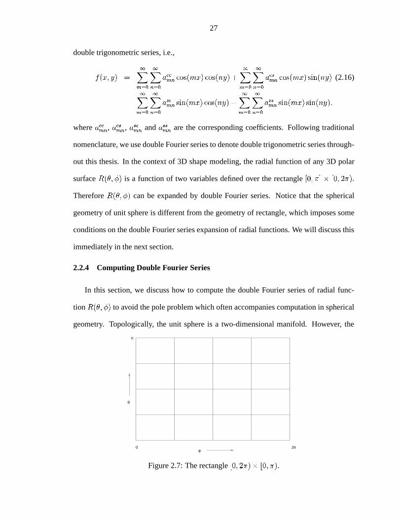
2.7 The rectangle[0; 2�)� [0; �). . . . . . . . . . . . . . . . . . . . . . . 27

2.8 Multi-resolution representation of an ellipsoid via the same order doubleFourier series and spherical harmonics. . . . . . . . . . . . . . . . . . . 31

2.9 Multi-resolution representation of a metasphere via the same order dou-ble Fourier series and spherical harmonics. . . . . . . . . . . . . . . . . 32

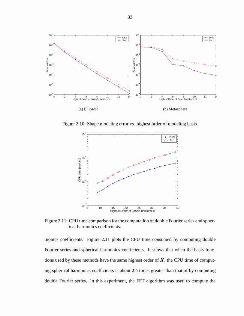
2.10 Shape modeling error vs. highest order of modeling basis. . . . .. . . . 33

2.11 CPU time comparison for the computation of double Fourier series andspherical harmonics coefficients. . . . . . . . . . . . . . . . . . . . . . 33

2.12 Two directions,(�1; �1) and(�2; �2), and the angle between them. . . 37

vii

2.13 An arbitrary point(�0; �0) onS2 and the curveS containing points thathave same angular distance to(�0; �0) . . . . . . . . . . . . . . . . . . . 38

2.14 A triangle with random orientations inIR2. . . . . . . . . . . . . . . . . 46

3.1 Shape modeling error vs. center shift for unit sphere. . . . . . . . . . . 49

3.2 Approximation off(r) by f1(r) under the conditionr � r0 � r0. Herer0 = 5 and� = 1. . . . . . . . . . . . . . . . . . . . . . . . . . . . . . 56

3.3 Segmentation data on a cross section of the ellipsoid,� = 0:2. . . . . . 60

3.4 Performance of the ellipsoid fitting center estimator. . . . . . . . . . . 62

4.1 Comparison of linear filtering and Wiener filtering results onS2. Redsurfaces represent the results of linear filtering and blue surfaces repre-sent the results of Wiener filtering. . . . . . . . . . . . . . . . . . . . . 66

4.2 Biases of a shape parameter estimator and a rotation angle estimator. . . 73

4.3 Comparison between the estimators’ standard deviations and the Cram´er-Rao bounds. . . .. . . . . . . . . . . . . . . . . . . . . . . . . . . . . 74

5.1 An grey level imageI, the set of edge pointsg detected inI, a propagat-ing contourf , andd(g;x) or d(g; f), the distance between the propagat-ing contour and its nearest edge point. . . .. . . . . . . . . . . . . . . 80

5.2 Interpretation of attraction potentialP . . . . . . . . . . . . . . . . . . 81

5.3 Motion of curve under curvature. The blue arrows represent negativecurvatures, while the red arrows represent the positive curvatures.. . . . 82

5.4 Standard deviation of reconstruction error vs.� for different shapes . . 91

5.5 Standard deviation of reconstruction error vs.� for different segmenta-tion noise levels . . . . . . . . . . . . . . . . . . . . . . . . . . . . . . 92

5.6 Reconstruction of an ellipsoid.. . . . . . . . . . . . . . . . . . . . . . 93

5.7 CT slices and the corresponding edge maps. . . . . . . . . . . . . . . 94

5.8 Contours solved with different� converge at different positions.. . . . 95

viii

5.9 Comparison of shape extraction results. (a) Local edge detector; (b)Active contour. . . . . . . . . . . . . . . . . . . . . . . . . . . . . . . 95

5.10 Segmentation results comparison between the active contours with andwithout volumetric penalization for edge blurred image . . . . .. . . . 96

6.1 CT-SPECT fusion results comparison for patients 62 . . . . . . . . . . 104

6.2 The net-count-maximization result for the patient with ID#7. Recon-structed SPECT slice corresponds to CT IM 41. . .. . . . . . . . . . . 105

6.3 The net-count-maximization result for the patient with ID#7. Recon-structed SPECT slice corresponds to CT IM 43. left) Result for fusionthat maximized counts in2 abdominal tumors. right) Result for fusionthat maximized counts in “big” which is unacceptable. . . . . .. . . . 107

A.1 Spherical harmonics. (a)jY ml (�; �)j, (b)<[Y m

l (�; �)] and=[Y ml (�; �)]. . 119

ix

LIST OF TABLES

Table

1.1 Properties of parametric and geometric active contours. (From [36]) . . 10

3.1 Shape modeling error vs. center shift for unit sphere. . . . . . . . . . . 48

4.1 The total number of nonzero entries in sparse mapping matrixK vs. thehighest oder of spherical harmonics basis. . . . . . . . . . . . . . . . . 66

6.1 Results from net-counts maximization for patients with pelvic tumors . 104

6.2 Results from net-counts maximization for patients with abdominal tumors 105

6.3 Results for patient (ID#7) with tumors in both the abdomen and pelvisfrom net-count maximization of all4 of his tumors. . . . . . . . . . . . 106

6.4 Results for counts in abdominal tumors for patient (ID#7) using differenttumors, or different tumor combinations, for the count maximization. . . 106

6.5 Results for counts in pelvic tumors for patient (ID#7) using differenttumor combinations for the count maximization. . .. . . . . . . . . . . 107

x

LIST OF APPENDICES

Appendix

A. Spherical Harmonics . . . . . . . . . . . . . . . . . . . . . . . . . . . . . 118

A.1 Spherical Harmonics . . . . . . . . . . . . . . . . . . . . . . . . 118A.1.1 Definition of Spherical Harmonics. . . . . . . . . . . 118A.1.2 Completeness of Spherical Harmonics . . . . . . . . . 119A.1.3 Addition Theorem . . . .. . . . . . . . . . . . . . . 120

A.2 Legendre Polynomial and Associated Legendre Function. . . . 121A.2.1 Legendre Polynomial . . .. . . . . . . . . . . . . . . 121A.2.2 Associated Legendre Function . .. . . . . . . . . . . 122

B. Statistics of Surface Function Extracted By Edge Filtering . . . . .. . . . 124

C. Derivation of Euler-Lagrange Equation . . . . . . . . . . . . . . . . . . . 127

xi

CHAPTER I

INTRODUCTION

1.1 Motivation

Enabled by the fast development of imaging techniques and computer hardware, there

has been an explosive growth of three-dimensional (3D) image data collected from all

kinds of physical sensors. The ability of a computer to properly understand and process

these image data has permitted many applications to problems in computer vision and

computer graphics. To achieve this ability, the first step is to extract object information

from the image data, which can be characterized as an object learning procedure in ma-

chine intelligence. Examples of useful object information include: shape; color; texture;

size; and its relative location to other objects in the scene. Such object information is

widely used in many image processing applications including: 3D cartoon animations;

video image processing; target detection in radar images; face recognition in security sys-

tems; and tumor dosimetry in nuclear medicine. For tasks geared toward object recognition

and reconstruction, shape models are widely studied and used due to their insensitivity to

changes in object color and surface texture, and their invariance to translation and scaling.

1

2

1.1.1 Statistical Shape Modeling

In the past two decades many shape modeling techniques have been developed for a

large variety of applications. The goal of shape modeling is to use as few parameters as

possible to describe as many shape details as possible. These two potentially conflicting

requirements arise in two of the primary tasks of shape modeling: 1) object recognition;

and 2) shape reconstruction. On the one hand, shape modeling should be parsimonious;

one should use as few model parameters as possible so that the 3D objects can be efficiently

stored and retrieved in object databases of manageable size for object matching and recog-

nition. On the other hand, for the purpose of visual reconstruction, shape modeling should

capture finer details, e.g., the high spatial frequencies in the shape. Development of classes

of shape models that can bridge the gap between recognition and reconstruction has been

an active research area in computer vision and computer graphics [34, 35, 54, 96, 99].

Although deterministic models are successfully employed in many applications, these

models are incapable of reflecting any noise or other random variations within a class of

shapes. In medical imaging, for instance, anatomical shape can change significantly dur-

ing a treatment. It is highly desirable to have reliable statistical shape models that can

characterize typical ranges of shape variation and capture meaningful statistical informa-

tion. This information can be used to develop optimal algorithms for noise removal, object

registration and segmentation, and establish tight bounds on achievable performance.

1.1.2 Image Segmentation and Registration in Medical Image Analysis

Heavily influenced by the fast development of image acquisition equipment, medi-

cal image analysis has evolved in the last twenty years from a multiplicity of directions.

Among all the techniques, image segmentation and multi-modal image registration are of

special interests to us because they are intensively used to quantify tumor activity in pa-

3

tients being treated by radiopharmaceutical therapy. Our research was partially supported

by a grant awarded by National Cancer Institute. The broad, long-term objectives of the

grant research are: 1)accurate tumor dosimetry from external imaging, and 2) effective-

and-resource-conserving treatment of patients with malignant follicular lymphoma by the

infusion of I-131 labeled anti-B1 monoclonal antibody (MAb) following infusion of a

predose of non-radioactive anti-B1 MAb.

Image segmentation is a fundamental task in medical image analysis. In segmentation,

objects of interest in the image are extracted so that we can analyze their properties. Such

properties can include pixel (voxel) intensities; centroid location; shape and orientation.

The information from object segmentations is routinely used in many different applica-

tions, such as: diagnosis [95]; treatment planning [65]; study of anatomical structure [33];

organ motion tracking [53]; and computer-aided surgery [5]. Object segmentation and

statistical shape modeling serve and rely on each other. Figure 1.1 illustrates such a rela-

tionship. On the one hand, object segmentation generates noisy surface data which can be

used to identify a shape model. On the other hand, statistical shape information acquired

through estimated parameters in a statistical shape model can guide the segmentation pro-

cedure. Other applications, such as object registration, shape denoising and shape classi-

fication, can be enhanced by accurate object segmentation and statistical shape modeling.

Due to noise and sampling artifacts in medical images, conventional edge detection

and thresholding techniques either fail to locate the object boundary or generate invalid

boundaries that must be removed in a post-processing step. Deformable models have been

developed to address these difficulties [27, 63, 77, 78]. Deformable models are curves and

surfaces defined within an image domain that can deform under different forces to locate

object boundaries. A more detailed description of deformable models will be given in

4

3D Image Data Sets

Object SegmentationNoisy Surface Data

Statistical Shape Modeling

Statistical Shape Information

Object Registration, Shape Denoising, Shape Classification, etc.

Figure 1.1: Relationship between image segmentation and shape modeling

Section 1.2.2. Although the existing deformable models can achieve satisfying results in

2D images, all of them have met difficulties in 3D imaging. The large number of voxels

in 3D images causes significant growth of computational complexity, which is intolerable

in most practical applications. This motivates us to find fast algorithms for 3D image

segmentation.

Image registration is a classical procedure in image processing and analysis. It aligns

two set of images so that corresponding coordinate points in the two images reflect the

same physical location of the scene or 3D volume being imaged. Usually, the two set of

images are obtained at different times, through different sensing systems, or from different

viewpoints, so matching the two images allows us to compare or integrate the information

contained in them. Due to the large diversity of data types in different applications, a

wide range of techniques has been developed for different applications. These techniques

can be classified either by the addressed registration problems or by the adopted method-

ologies. A good survey of these techniques is given in [17]. The focal application in

this research is multi-modal medical image registration for tumor activity quantification.

In this application, we must integrate structural information from computed tomography

5

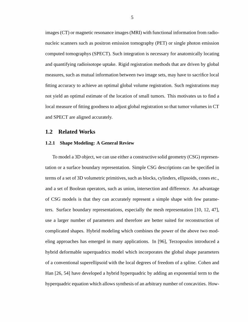
images (CT) or magnetic resonance images (MRI) with functional information from radio-

nucleic scanners such as positron emission tomography (PET) or single photon emission

computed tomographys (SPECT). Such integration is necessary for anatomically locating

and quantifying radioisotope uptake. Rigid registration methods that are driven by global

measures, such as mutual information between two image sets, may have to sacrifice local

fitting accuracy to achieve an optimal global volume registration. Such registrations may

not yield an optimal estimate of the location of small tumors. This motivates us to find a

local measure of fitting goodness to adjust global registration so that tumor volumes in CT

and SPECT are aligned accurately.

1.2 Related Works

1.2.1 Shape Modeling: A General Review

To model a 3D object, we can use either a constructive solid geometry (CSG) represen-

tation or a surface boundary representation. Simple CSG descriptions can be specified in

terms of a set of 3D volumetric primitives, such as blocks, cylinders, ellipsoids, cones etc.,

and a set of Boolean operators, such as union, intersection and difference. An advantage

of CSG models is that they can accurately represent a simple shape with few parame-

ters. Surface boundary representations, especially the mesh representation [10, 12, 47],

use a larger number of parameters and therefore are better suited for reconstruction of

complicated shapes. Hybrid modeling which combines the power of the above two mod-

eling approaches has emerged in many applications. In [96], Terzopoulos introduced a

hybrid deformable superquadrics model which incorporates the global shape parameters

of a conventional superellipsoid with the local degrees of freedom of a spline. Cohen and

Han [26, 54] have developed a hybrid hyperquadric by adding an exponential term to the

hyperquadric equation which allows synthesis of an arbitrary number of concavities. How-

6

ever, these hybrid models rely on strong assumptions on the form of the object and need

considerable human interaction for computation of the special parameters to characterize

the local detail.

Fourier descriptors of surface boundaries have emerged as powerful alternatives to

the above models. This kind of model represents the shape of polar surfaces in a linear

combination of orthonormal basis functions and provides a radial surface description with

respect to a selected origin inside the object. The basis functions are not limited to si-

nusoids; other orthogonal polynomials, such as spherical harmonics, are possible too. In

[86], Persoon and Fu introduced Fourier descriptors for 2D curve representation. Staib

and Duncan [92, 93] extended the technique of [86] to deformable templates in both 2D

and 3D, and applied them to boundary localization. In [76], Matheny compared the er-

rors of fitting various surface harmonics to an assortment of synthetic data and real range

data obtained from laser scan of surfaces. In [53], anatomical shapes were studied and

modeled by spherical harmonics. Fourier descriptors are attractive because they have the

following features. First, the sets of Fourier basis functions are complete over the space

of polar surfaces. Therefore any continuous and finite surface can be expanded as a linear

combination of the countably infinite Fourier basis functions. Second, the basis functions

are linear independent, which makes the corresponding parameters in the decomposition

unique. Third, the basis functions are ordered in spatial frequency. This facilitates hierar-

chical “multi-resolution” shape decomposition where the truncation of the series controls

the smoothness of the reconstruction. These properties make Fourier descriptors very use-

ful both in object recognition and shape reconstruction. In object recognition, low order

coefficients can be kept. The objects can be easily stored and retrieved in the databases

because of the small size and hierarchical organization of the data structure. In the shape

reconstruction problem, we can easily determine the truncation points according to a user-

7

specified accuracy requirement. There are two disadvantages of Fourier descriptors. One

is that object center has to be estimated in advance. Another is that a large number of

parameters must be employed to recover very fine details of the object because Fourier

descriptors use global basis functions.

Many researchers have explored the area of statistical shape modeling [30, 45, 93,

103, 115]. The common procedure of these approaches is as follows: First extract shape

features or shape parameters from training data sets. These features may include labeled

“landmark” points [30, 45]; coefficients of the Fourier series [93]; or distance map [71].

Next, compute the mean and variance of the shape or shape parameters from the features

extracted in the first step. Usually principle component analysis (PCA) is used to compute

variance and characterize typical variations of the shape. Finally, the statistical properties

of the shape are incorporated into a image processing algorithm to accomplish registration

and segmentation.

Our approach is related to Staib’s deformation model [93, 103] since we also use

Fourier series as basis functions to model 3-D shapes. The novelty of our approach lies

in treating the coarse segmentation result as a random field over the unit sphere and us-

ing the spectral theory of random fields over the sphere to obtain statistically uncorrelated

shape parameters. Since 1950’s, mathematicians have studied random field models for

applications in earth science, astrophysics and electrical field theory [1]. Image process-

ing researchers have used random field models for texture synthesis and classification

[116, 40], and image segmentation [115]. Curiously, in shape modeling and analysis, ran-

dom field models have not been widely studied. In this thesis, we propose an isotropic

random field model for randomly oriented 3D star-shaped objects using spherical harmon-

ics as the eigen-functions in a Karhunen-Lo´eve expansion of the random field. Based on

the spectral theory of isotropic random fields, we address two problems. The first one

8

is optimal shape filtering: given noisy samples of surface boundary points, e.g. coarsely

segmented from an object, find an optimal estimate of the true surface boundary. Using

Wiener filtering theory, an orthogonal representation of random fields is applied to find

the linear minimum mean square error surface estimator. The second problem is the 3D

object registration problem. In [19] and [20], Burel proposed that spherical harmonics can

be used to decompose 3D shapes to get invariants for object orientation estimation. Based

on Burel’s method and the statistical shape model developed in this thesis, we design a

maximum likelihood estimator which can simultaneously estimate the spherical harmonic

coefficients and register two 3D objects of different orientations.

We next turn to the problem of selecting the origin in the polar object representation.

The accuracy and efficiency of Fourier descriptors are highly dependent on the choice of

origin in the coordinate system. In [76], an ellipsoid fitting method was shown to be a good

center estimation method for convex shapes. To link the accuracy of center estimation with

the accuracy of shape modeling, we study the statistical properties of the center estimator.

Both our theoretical derivation and our experimental results show that this center estimator

is an efficient maximum likelihood estimator under low power Gaussian noise condition.

1.2.2 Image Segmentation and Registration

As pointed out in a survey by McInerney [77], deformable models (active contours)

offer a unique and powerful approach to image analysis that combines geometry, physics,

and approximation theory. Furthermore, the application of deformable contour models to

segment structures in 2D and 3D images have recently enabled many advances in medical

image analysis [22, 21, 27, 26, 52, 63, 75, 78, 108].

There are basically two types of deformable models (active contours): parametric de-

formable models [27, 26, 52, 63, 78, 108] and geometric deformable models [22, 21, 75].

9

The class of parametric deformable models originates from the “snake” introduced by

Kass [63] which uses an energy-minimizing curve to locate boundaries in 2D imagery.

The curve is obtained by solving an optimization problem to minimize the sum of an inter-

nal energy function, which penalizes curve roughness in the model, and an external energy

function which attracts the curve to object boundary. Any modeling approach applied to

this class must deal with sensitivities to initialization and noise. Different approaches

adopt different internal and external energy functions. Chapter V will discuss the internal

and external functions in detail for both 2D and 3D images. The geometric deformable

models were proposed independently by Caselles in [21] and by Malladi in [75]. These

methods are based on iterative optimization via the theory of curve evolution and are im-

plemented via level set techniques. Unlike parametric active contours, which represent the

contour explicitly as parameterized curves or surfaces, geometric active contours repre-

sent the evolving contour implicitly by a special level set function. This kind of evolving

contour can split and merge freely without previous knowledge of the number of objects

in the scene. In other words, such an evolving contour can handle the topology change

automatically. The disadvantage of geometric active contours is that their computational

complexity is much higher than that of parametric active contours. The level set function

used by geometric active contour is defined over a 2D (3D) grid in the image plain (vol-

ume). In every evolution iteration, the geometric active contour method has to update the

level set function at every grid point or at least at the grid points in a narrow band near the

propagating front, which causes a heavy computational burden. This technique is espe-

cially burdensome for 3D images. Table 1.2.2 is taken from [36], which summarizes the

advantages and disadvantages of parametric deformable models and geometric deformable

models.

Although parametric deformable models usually have lower computational complexity

10

Table 1.1: Properties of parametric and geometric active contours. (From [36])Parametric Contours Geometric Contours

Efficiency ? ? ? ?Ease of Implementation ? ? ? ??

Topology Change No YesOpen Contours Yes No

Interactivity Good Poor

than geometric deformable models, they are still not very efficient in solving 3D segmen-

tation problems. Parametric deformable models are implemented through minimizing an

energy function via variational principles, which often leads to solving partial differen-

tial equations (PDE) for the surface function. Iterative methods, such as finite element

methods (FEM) [27] and finite difference methods (FDM) [108] have been used to solve

PDE’s involved in this optimization problem. However, FEM/FDM have met difficulties

for 3D imaging applications. The large number of voxels in 3D images causes significant

growth of computation time which is intolerable in most practical applications. It is well

known that spectral methods have a faster rate of convergence than that of FDM and FEM

in solving PDE’s [50]. This motivates us to explore the application of spectral methods to

reduce the computation time for 3D deformable models. Based on the spherical geometry

of star-shaped surfaces, we propose to use double Fourier series to solve the PDE defined

over the unit sphere. The method is applied to segment both synthesized 3D images and

X-ray CT images. It is shown that the new method preserves the merits of other paramet-

ric active contour methods while significantly reducing the computation time. Due to the

generality of our mathematical formulation, the method can be easily applied to solve the

surface reconstruction problem.

Over the past three decades, the very active research in the area of image registration

has produced several different registration methods. The fundamental task of image reg-

11

istration is to find the spatial transformation needed to properly overlay two images. As

explained in [17], this task can be decomposed into four major steps. The first step is

to decide on the feature space to use for matching the images. Examples of commonly

used features include: image intensities; extracted edges; corners; line intersections and

centroids. The second step is to choose a similarity measure which evaluates the closeness

of the feature set extracted from each image. The third step is to parameterize the spatial

transformation. And the fourth step is to specify the searching strategies over these pa-

rameters in order to maximize the similarity measure. Two broad categories of registration

techniques can be identified. First are those techniques that are based on salient features or

surface, such as control-point matching or surface correlation. Here some form of anatom-

ical structures has to be identified or segmented before registration. Salient features refer

to specific pixels in the image which contain information indicating the presence of an eas-

ily distinguished meaningful characteristic in the image. The second category is based on

matching image pixel (voxel) intensities. This category includes mutual information (MI)

based registration techniques [100], which minimize the entropy of the joint histogram of

grey level values of the two images. Both control-point matching [18, 49, 69, 74, 79] and

pixel intensity techniques [28, 80, 100] are in common use for clinical applications.

For applications of radiotherapy treatment planning and response monitoring, it is of-

ten necessary to fuse SPECT and CT data sets so that the functional information and

anatomical information can be integrated. Due to the low spatial resolution of SPECT, the

ultimate accuracy of the estimate of tumor activity in therapy patients using CT-SPECT

fusion is difficult to establish. Inaccuracy can be caused by “registration error” which in

turn comes from several factors. Depending on the type of registration used, these factors

include: 1) a non-rigid change in the body habitus between CT and SPECT, 2) a change

in the tumor location relative to the large organs or relative to the skin markers, 3) a poor

12

choice of the control points that initialize a mutual information (MI) based registration, 4)

a non-optimum choice of other parameters in MI registration, 5) a failure of maximum MI

to yield a good registration even with the optimal choice of input parameters. In our appli-

cation, we have noticed that a tumor volume of interest (VOI) from CT sometimes does not

perfectly overlay the true position of the tumor in the SPECT image set. Furthermore, the

magnitude of the difference between the activity estimate from the MI registration proce-

dure and that from a perfect overlay is uncertain. As alternative, we explore the possibility

of optimizing the estimate of tumor location and orientation with respect to within-VOI

activity quantification. Control points matching or mutual information based registration

is used to obtain an initial rigid transformation between CT and SPECT. A local opti-

mization is then performed to fine tune the initial global registration, with the criterion of

maximizing counts in VOIs of known tumors. The local optimization appears to be more

resistant to overlay errors.

1.3 Thesis Contributions

The original contributions made by this dissertation are summarized as follows.

� We have compared two Fourier descriptors of 3D polar shapes and studied the re-

lated computational issues.

� We have developed a statistical shape model using the spectral theory of isotropic

random field. We have proved that if the orientation of a 3D polar object is uniformly

distributed inSO(3), the observed radial function of this 3D object is an isotropic

random field over the unit sphereS2.

� For center estimation problem, we have established that the estimator of the ellipsoid

parameter vector proposed by Bookstein is a maximum likelihood estimator when

13

the segmentation noise is Gaussian with low variance. A lower bound has also been

derived for the variance of the center estimator under a Gaussian segmentation noise

model.

� We have proposed a statistical shape model and a Wiener filtering strategy for opti-

mal shape filtering.

� We have developed a maximum likelihood method to jointly estimate shape param-

eters and 3D rotation angles based on an isotropic Gaussian noise model.

� We have developed a fast algorithm for 3D object segmentation and surface recon-

struction by applying spectral methods to solve elliptic PDE’s over the unit sphere.

We have introduced volumetric penalization to prevent contour leaking at broken

boundaries or spurious edges.

� We have proposed a refinement of MI-based rigid CT-SPECT registration which

enhances robustness by maximizing counts in segmented volumes of interest.

1.4 Organization of Thesis

This thesis is organized as follows. In Chapter II, we study spherical harmonics and

double Fourier series on the sphere as two Fourier descriptors of surface boundaries. Re-

lated computational issues are discussed. The two descriptors are compared in terms of

convergence rate and shape modeling accuracy. Chapter II also studies the statistical prop-

erties of the segmentation error and develops an orthogonal representation of isotropic

random field over the unit sphere. The detailed proof of the Karhunen-Lo´eve expansion

formula is also given in this chapter. In Chapter III, we investigate the center estimation

problem for 3D shape. The ellipsoid fitting method proposed by Bookstein is described

14

and shown to be a maximum likelihood estimator of ellipsoid parameters when the seg-

mentation noise level is low. A lower bound is derived to evaluate the performance of

the ellipsoid fitting center estimator. In Chapter IV, two applications of statistical shape

models are presented. The first application is Wiener filtering of a noisy surface boundary.

The second application is joint estimation of shape parameters and 3D rotation angles by

maximum likelihood. In Chapter V, a fast algorithm for 3D surface reconstruction and

object segmentation is developed based on our shape modeling approach and solving PDE

by double Fourier series expansion methods. A volumetric penalization term is introduced

in the PDE to prevent contour leakage at broken or blurred boundaries. The segmentation

is evaluated for both real medical images and synthesized images. Chapter VI proposes an

adjustment to rigid CT-SPECT registration so as to better quantify tumor uptakes. Finally,

Chapter VII contains conclusions and directions of future work related to this research.

CHAPTER II

STATISTICAL POLAR SHAPE MODELING BYFOURIER DESCRIPTORS

2.1 Introduction

Techniques of three dimensional shape modeling have been widely studied over the

past two decades [9][30][93] [115][103]. Generally speaking, shape modeling is a funda-

mental process of combining physical measurement of objects with a mathematical model.

In many computer vision related areas, such as pattern recognition, deformation and mo-

tion analysis, image registration and image retrieval, shape modeling techniques have been

integrated with other techniques to achieve different goals. Models widely used in these

applications include constructive solid geometry and surface boundary representations. In

the rest of this thesis, “shape modeling” refers to surface boundary representations. De-

terministic surface descriptions, such as polygons, B-splines and Fourier descriptors, have

been well established [9]. Among these descriptions, the parametric representations that

are object-centered and use a linear combination of basis functions, are of special interest

to us. These mappings from spatial object space to parameter space provide a compact

representation of the object and are useful for shape storage and reconstruction, noise fil-

tering, and pattern recognition.

In this chapter, we investigate the properties of spherical harmonics and double Fourier

15

16

series as two Fourier descriptors for 3D polar shape modeling. We investigate both deter-

ministic and statistic formulations of polar surface approximation. This chapter is orga-

nized as follows. Section 2.2 discusses the theoretical expression and computational issue

of spherical harmonics and double Fourier Series. These two descriptors are compared

in terms of convergence rate and shape modeling accuracy. Section 2.3 studies the sta-

tistical properties of the segmentation error and develops the orthogonal representation of

isotropic random fields for statistical shape modeling. The detailed proof of the spectral

theory is also given in this section. As it will be shown in Chapter IV, the spectral rep-

resentation of isotropic random field can be applied to several tasks in image processing

such as: Wiener filtering; shape classification; and object registration.

2.2 Deterministic Polar Shape Modeling by Fourier Descriptors

The main process of 3D deterministic shape modeling includes the following steps:

1) find the proper basis functions; 2) sample the 3D object surface; 3) compute the shape

parameters through sampling data. The surface of a polar shape (star shape) object can be

represented by its radial coordinater with respect to a selected origin inside the object.r

is a single value function of� and�, where(�; �) is a direction vector on the unit sphere.

The unit sphere is defined as the sphere of radius 1 and centered at origin. Hereafter the

unit sphere will be denoted byS2, and coordinates onS2 will be described by(�; �) or

x, i.e. (�; �) 2 S2 or x 2 S2. To be accurate, 3D polar shapes are defined as shapes that

have a boundary function in the form off : S2 ! [0;1]. Figure 2.1 illustrates polar and

non-polar shapes in 2D.

Fourier descriptors represent polar shape objects as a linear combination of orthonor-

mal basis functions. In the following, we will study shape modeling by spherical harmon-

ics and double Fourier series over the unit sphere.

17

Or

(a) polar shape

O

r

(b) non-polar shape

Figure 2.1: Surface boundaries of star shape and non-star shape objects.

2.2.1 Spherical Harmonics

Spherical harmonicsfY ml (�; �)g are special functions defined on the unit sphere [3] as

Y ml (�; �) = (�1)m

s2l + 1

4�

(l �m)!

(l +m)!Pml (cos �)eim� (2.1)

where� 2 [0; �] is the polar angle,� 2 [0; 2�] is the azimuthal angle,Pml (x) is the

associated Legendre function [Appendix A.2],l is a non-negative integer,m is an integer

in [�l; l], and the normalization is chosen such thatZ 2�

0

Z �

0

Y ml (�; �)Y m0�

l0 (�; �) sin �d� d� = Æl;l0Æm;m0 : (2.2)

HereY � is the complex conjugate ofY , andÆm;m0 is the Kronecker delta function defined

as the following

Æm;m0 =

8><>:1 if m = m

0

;

0 otherwise.(2.3)

Figure 2.2 shows the polar angle� and the azimuthal angle� on the unit sphere.

Spherical harmonics are the angular portion of the solution to the Laplace equation

in spherical coordinates, where azimuthal symmetry is not present [3] [Appendix A.1].

They are orthonormal and ordered in spatial frequency as a function ofl andm. The set

18

θ

φ

x

y

z

Figure 2.2: Direction vector(�; �) on the unit sphere.� is the polar angle and� is theazimuthal angle.

of spherical harmonics is also complete in the space of continuous functions overS2 of

finite energy. Therefore, any radial functionf : S2 ! IR, of polar shape object, can be

expanded as a linear combination of spherical harmonics:

f(�; �) =1Xl=0

lXm=�l

Cml Y

ml (�; �) (2.4)

where the coefficientsCml are uniquely determined by

Cml =

Z �

0

Z 2�

0

Y m�l (�; �)f(�; �) sin �d� d�: (2.5)

The right hand side of (2.4) is called the Laplace series, which converges uniformly. The

sufficient conditions for the spherical harmonic expansion are given by Hobson in [59].

The corresponding series coefficientsCml are the shape model parameters. Since the values

of surface functions are always real, the real and imaginary parts of shape parameters are

constrained by the following relations:

<fCml g =

8><>:�<fC�m

l g m odd

<fC�ml g m even

(2.6)

19

=fCml g =

8><>:=fC�m

l g m odd

�=fC�ml g m even

(2.7)

2.2.2 Computing Laplace Series

As well known by all practitioners, computational complexity is always a big concern

in 3D shape modeling. In this subsection, we discuss the computational complexity and the

accuracy of modeling 3D polar shapes by spherical harmonics. Two different algorithms

to compute the Laplace series, SVD and FFT, are compared in terms of complexity and

accuracy.

2.2.2.1 SVD

Using singular value decomposition (SVD) to find the coefficients of spherical har-

monics in the sense of least squared error was proposed in [41] and [76]. Letr(�; �)

denote the sample value of the radial coordinate in the direction(�; �) andR(�; �) denote

the radial function of the reconstructed shape using spherical harmonics. The least squared

error approach requires the minimization of the following error function:

e =X

(�;�)2S0[r(�; �)� R(�; �)]2 (2.8)

whereS0 � S2 is the sample set.

The functionR(�; �) is a Laplace series with complex coefficients. SinceY ml (�; �)

is a complex function andY �ml (�; �) = (�1)mY m�

l (�; �), the real and imaginary parts

of Y ml (�; �), i.e. <fY m

l (�; �)g and=fY ml (�; �)g, are often used as basis functions in

place ofY ml (�; �) andY �m

l (�; �) to simplify the computation. The functionsUml (�; �)

�=

<fY ml (�; �)g andV m

l (�; �)�= =fY m

l (�; �)g are also called Tesseral harmonics. Then, the

reconstructed shape can be represented as

R(�; �) =KXl=0

lXm=0

Aml Um

l (�; �) +Bml V m

l (�; �): (2.9)

20

whereAml andBm

l are the coefficients of real values, andK is the highest order of basis

functions in the shape modeling, which controls the fineness of surface detail that can be

handled. The choice ofK affects not only the modeling accuracy, but also the compu-

tational complexity for estimating the coefficientsfAml g andfBm

l g. The total number

of coefficients is(K + 1)2 in equation (2.9). If the maximum likelihood method is em-

ployed to estimate the coefficients, which is essentially a nonlinear iterative optimization

procedure, the computational complexity will be too high for large value ofK. Users

have to properly balance the accuracy of shape modeling and the amount of computation

according to necessities in their applications.

A group of linear equations can be obtained if we write the equation (2.9) for every

sampling direction(�i; �i), wherei is the index of the sample set. Write them in matrix

format, we have

r = Ua +Vb: (2.10)

wherer = (r(�1; �1); : : : ; r(�i; �i); : : : ; r(�N ; �N))T , (�i; �i) 2 S0 is a vector representing

sampled surface values,a = (A00; A

01; A

11; A

02; A

12; A

22; : : : ; A

KK)

T andb = (B00 ; B

01 ; B

11 ; B

02 ; B

12 ; B

22 ; : : : ; B

KK

are coefficients vectors to be estimated,U andV are matrices withUml (�i; �i) andV m

l (�i; �i)

as their entries. For instance,U has the form as following:

U =

0BBBBBBBB@

U00 (�1; �1) U0

1 (�1; �1) U11 (�1; �1) � � � UK

K (�1; �1)

U00 (�2; �2) U0

1 (�2; �2) U11 (�2; �2) � � � UK

K (�2; �2)

......

.... . .

...

U00 (�N ; �N) U0

1 (�N ; �N) U11 (�N ; �N) � � � UK

K (�N ; �N)

1CCCCCCCCA: (2.11)

LetX = (U;V) andc = (a;b)T , we can rewrite equation ( 2.10) in the form:

r = Xc: (2.12)

In this way, all shape parameters are put into a single vector and can be solved simulta-

21

neously by SVD method. In case where the number of sample points is greater than the

number of parameters, the system is calledover-determined. For over-determined sys-

tems, SVD provides a solution for the parameters that is the best approximation in the

least square error sense. We can coarsely analyze the computational complexity of SVD

method. LetN be the number of sampling points overS2. To set up the matrixX, the

spherical harmonics have to be computed at theN sampling points, which has a complex-

ity of at leastO(N2) for non-uniformly distributed sampling points. The SVD procedure

usually hasN3 arithmetic operations. Therefore the computational complexity of this

method should be aroundO(N3).

2.2.2.2 FFT

The spherical harmonic expansion is an extension of the special Fourier transform on

unit sphere. Some researchers have explored fast algorithms similar to the 2D FFT for this

expansion [37, 55, 89]. Although spherical harmonics comprise an orthogonal set in the

continuous space, they are not orthogonal in discrete cases, such as for the sampled data.

To approximate them by an orthogonal set on a discrete domain, we must associate them

with weight functions. The difference and analogy of spherical harmonics orthogonal on

a discrete set of points on the sphere were studied in [82]. This work makes it possible to

adapt FFT analysis to spherical harmonics. It is desirable to sample a band-limited radial

function in such a way that the original shape can be exactly recovered from the samples.

In [39], Driscoll and Healy developed a sampling theorem and a fast algorithm to reduce

the computational complexity of spherical harmonics for band-limited functions on unit

sphere. The bandwidth was defined in terms of the highest order of spherical harmonics

which have a non-zero coefficient.

Theorem 1 (Sampling Theorem overS2 [39]) Letf(�; �) be a band-limited function on

22

S2 such thatfml = 0 for l � b. Then

fml =

p2�

2b

2b�1Xj=0

2b�1Xk=0

a(b)j f(�j; �k)Y

m�l (�j; �k); (2.13)

for l < b and jmj � l. Herefml is the spherical harmonic coefficient off , �j = �j=2b,

�k = �k=b, and the coefficientsa(b)j are determined by the equation

a(b)0 Pl(cos �0) + a

(b)1 Pl(cos �1) + � � �+ a

(b)2b�1Pl(cos �2b�1) =

p2Æl;0: (2.14)

The fast algorithm was named as “FFT” overS2 and has a computational complexity of

O(N(logN)2). We will compare its performance with SVD method in the next section.

2.2.2.3 Experimental Results

As aforementioned, both the SVD method and the FFT method can be employed to

compute the coefficients in the spherical harmonic expansion. We compare their charac-

ters and performance by some experiments. All the computation in the experiment was

completed on a Sun Ultra-10 workstation via MATLAB. Four different shapes are mod-

eled by spherical harmonics basis in our experiments. Three of them have global implicit

expressions as:( x10)2 + (y

9)2 + ( z

7)2 = 1, x4 + y4 + z4 = 1 and( x

10)6 + (y

9)6 + z6 = 1.

The last one is the surface of a 3D medical organ, a liver manually segmented from X-ray

CT image. Figure 2.3 shows these shapes. Notice that some sharp corners of the liver are

missing in the shape of liver due to the finite number of spherical harmonic functions used

in the model. The normalized residual error of shape modeling is defined as following

err(K) =

qPN�1i=0

PM�1j=0 [r(�i; �j)�RK(�i; �j)]2=(NM)PN�1i=0

PM�1j=0 r(�i; �j)=(NM)

; (2.15)

whereK is the highest order of spherical harmonics employed,�i = i �N

, �j = j 2�M

, r(�; �)

andRK(�; �) represent the original shape and the reconstructed shape respectively. err(K)

is solely caused by the truncation of the Laplace series. For shapes with limited spatial

23

frequency, such as the unit sphere, err(K) vanishes whenK is greater than the radial

function bandwidth.

(a) (b) (c) (d)

Figure 2.3: 3D shapes used in the shape modeling experiments: (a)( x10)2+(y

9)2+( z

7)2 = 1;

(b) x4 + y4 + z4 = 1; (c) ( x10)6 + (y

9)6 + z6 = 1; (d) Segmented liver modeled

by spherical harmonics,K = 14

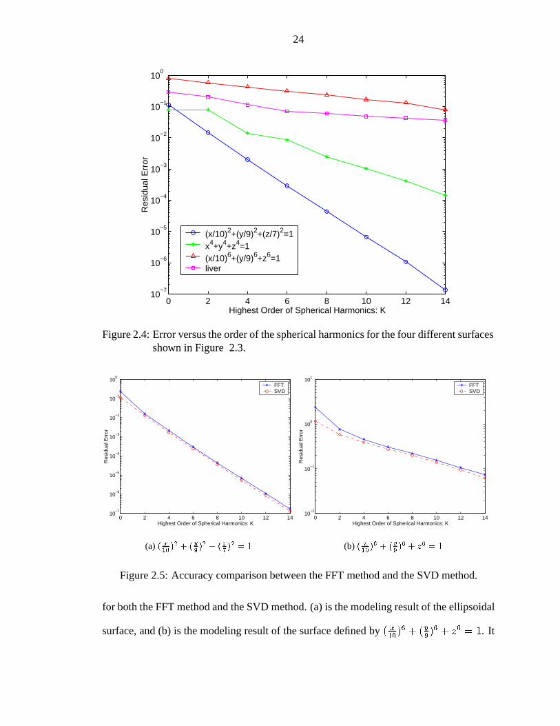
First, we test modeling accuracies for different shapes. Figure 2.4 shows the residual

error of shape modeling versus the highest order of spherical harmonics employed in the

SVD method. It can be seen that the residual errors decrease exponentially withK, the

highest order of spherical harmonics used. As expected, the decreasing speed is shape

dependent. The more irregular the shape is, the slower is the decreasing speed of the

residual modeling error. Using spherical harmonics with the highest order asK = 14, the

residual error is1:37 � 10�7 for the ellipsoidal surface,1:45 � 10�4 for the shape defined by

x4 + y4 + z4 = 1, 3:74 � 10�2 for the medical organ liver, and7:95 � 10�2 for the shape

defined by( x10)6 + (y

9)6 + z6 = 1. One can expect the representation order needed for

relevant 3D polar medical objects to be in the range10 � K � 20, and the corresponding

magnitudes of residual error be in the range from10�4 to 10�2.

In the second experiment, we compared the accuracies of FFT method and SVD

method. The same surface sampling data was used by these two methods. Figure 2.5

plot the residual error of shape modeling versus the highest order of spherical harmonics

24

0 2 4 6 8 10 12 1410

−7

10−6

10−5

10−4

10−3

10−2

10−1

100

Highest Order of Spherical Harmonics: K

Res

idua

l Err

or

(x/10)2+(y/9)2+(z/7)2=1x4+y4+z4=1(x/10)6+(y/9)6+z6=1liver

Figure 2.4: Error versus the order of the spherical harmonics for the four different surfacesshown in Figure 2.3.

0 2 4 6 8 10 12 1410

−7

10−6

10−5

10−4

10−3

10−2

10−1

100

Highest Order of Spherical Harmonics: K

Res

idua

l Err

or

FFTSVD

(a) ( x10)2 + (y

9)2 + ( z

7)2 = 1

0 2 4 6 8 10 12 1410

−2

10−1

100

101

Highest Order of Spherical Harmonics: K

Res

idua

l Err

or

FFTSVD

(b) ( x10)6 + (y

9)6 + z6 = 1

Figure 2.5: Accuracy comparison between the FFT method and the SVD method.

for both the FFT method and the SVD method. (a) is the modeling result of the ellipsoidal

surface, and (b) is the modeling result of the surface defined by( x10)6 + (y

9)6 + z6 = 1. It

25

2 4 6 8 10 12 14 1610

−2

10−1

100

101

102

Highest Order of Spherical Harmonics: K

CP

U T

ime

(sec

ond)

FFTSVD

Figure 2.6: CPU time comparison for the SVD method and the FFT method.

can be seen that for the same value ofK, the errors of SVD and FFT have the same order

of magnitude, although the one for the SVD method is slightly smaller. This is because

the FFT method requires the function to be band-limited which may not be true for an

arbitrary polar surface function. When a shape contains spatial frequencies that have to be

modeled by spherical harmonics higher thanK, there will be aliasing phenomenon in the

FFT method.

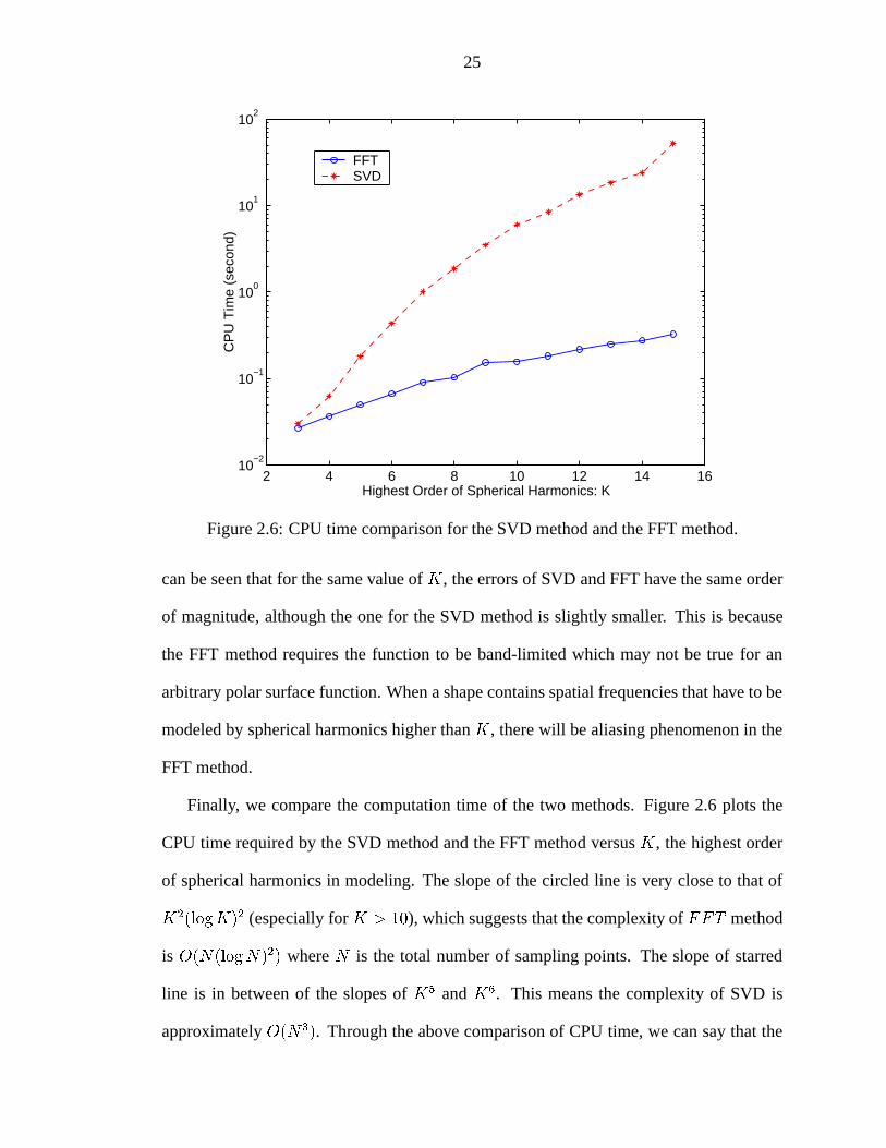
Finally, we compare the computation time of the two methods. Figure 2.6 plots the

CPU time required by the SVD method and the FFT method versusK, the highest order

of spherical harmonics in modeling. The slope of the circled line is very close to that of

K2(logK)2 (especially forK > 10), which suggests that the complexity ofFFT method

is O(N(logN)2) whereN is the total number of sampling points. The slope of starred

line is in between of the slopes ofK5 andK6. This means the complexity of SVD is

approximatelyO(N3). Through the above comparison of CPU time, we can say that the

26

computational complexity of SVD method is much higher than that of FFT method.

The following conclusions can be drawn for shape modeling by spherical harmonic

functions:

➀ For normal 3D polar shape objects, i.e., not as irregular as( x10)6 + (y

9)6 + z6 = 1,

the highest order of spherical harmonics needed for modeling is in the range10 �

K � 20, and the magnitude of modeling error will be in the range(10�6; 10�3).

➁ The SVD method and the FFT method give similar modeling accuracy if the surface

sampling data sets used by two methods are same.

➂ The FFT method requires the sampling points to be uniformly distributed on� and

�. It has very low computational complexity.

➃ The SVD method has the advantage that the sampling points can be arbitrarily dis-

tributed on the sphere. This allows to apply a higher sampling rate in surface areas

of large Gaussian curvatures, and a lower sampling rate for relatively flat areas.

However, its computational complexity is much higher than that of the FFT method.

2.2.3 Double Fourier Series

The simplest form of double Fourier series (DFS) arises in an expansion of scalar

functions of two variables over a rectangular domain[a; b] � [c; d]. The basis functions

of such a DFS are separable, i.e. a product of two sets of 1-D basis functions on[a; b]

and[c; d], respectively. When these two sets of basis functions are complex trigonometric

systems, an arbitrary functionf(x; y) defined in this rectangle can be decomposed into a

27

double trigonometric series, i.e.,

f(x; y) =1Xm=0

1Xn=0

accmn cos(mx) cos(ny) +1Xm=0

1Xn=0

acsmn cos(mx) sin(ny) (2.16)

1Xm=0

1Xn=0

ascmn sin(mx) cos(ny) +1X

m=0

1Xn=0

assmn sin(mx) sin(ny):

whereaccmn, acsmn, ascmn andassmn are the corresponding coefficients. Following traditional

nomenclature, we use double Fourier series to denote double trigonometric series through-

out this thesis. In the context of 3D shape modeling, the radial function of any 3D polar

surfaceR(�; �) is a function of two variables defined over the rectangle[0; �] � [0; 2�).

ThereforeR(�; �) can be expanded by double Fourier series. Notice that the spherical

geometry of unit sphere is different from the geometry of rectangle, which imposes some

conditions on the double Fourier series expansion of radial functions. We will discuss this

immediately in the next section.

2.2.4 Computing Double Fourier Series

In this section, we discuss how to compute the double Fourier series of radial func-

tionR(�; �) to avoid the pole problem which often accompanies computation in spherical

geometry. Topologically, the unit sphere is a two-dimensional manifold. However, the

0 2π

π

φ

θ

Figure 2.7: The rectangle[0; 2�)� [0; �).

28

geometry of sphere is fundamentally different from that of the rectangle shown in Fig-

ure 2.7. For example, the surface of a torus is also defined over[0; �] � [0; 2�] and can

be unwrapped into a cylinder, then into a rectangle, but the surface of sphere can not be

unwrapped in such a way into a rectangle [14].

The difficulty in applying DFS to polar shapes is due to the boundary conditions im-

posed at the two poles(�; �) 2 f(0; �); (�; �)g. First, the radial functionR(�; �) is ex-

panded by a 1-D Fourier series in longitude with truncationM ,

R(�; �) =MX

m=�MRm(�)e

im�; (2.17)

whereRm(�) =1K

PK�1k=0 R(�; �k)e

�im�k , �k = 2�k=K andK = 2M . Next, we expand

Rm(�) in a Fourier series that accounts for the pole boundary conditions at� = 0; �. These

boundary conditions are [14]:

Rm(�) =

8><>:finite; m = 0;

0; m 6= 0;

(2.18)

d

d�Rm(�) =

8><>:finite; oddm;

0; evenm:(2.19)

The condition onRm(�) is to ensure that the approximatedf(�; �) is continuous at poles,

while the condition ondd�Rm(�) is to avoid second-order poles in applying spectral method

to solve Laplace equation over the unit sphere [83]. If we use sine or cosine series alone

as basis functions to expandRm(�), they will not meet the above boundary conditions.

For example, letRm(�) =P

nRn;m cosn�. Whenm is odd,Rm(�) sin(m�) will be

discontinue at the poles unless some additional constraints are imposed onRn;m [8, 111,

112].

29

In [25] Cheong proposed the following expansion

Rm(�) =PJ�1

n=0 Rn;0 cosn�; m = 0;

Rm(�) =PJ

n=1Rn;m sinn�; oddm; (2.20)

Rm(�) =PJ

n=1Rn;m sin � sinn�; evenm 6= 0:

Cheong’s expansion ofRm(�) does not make explicit use of the cosine series for evenm

and avoids the imposition of a constraint that the sum of expansion coefficients should

vanish. We adopt this expansion in our approach.

To avoid possible singularities arising from dividing bysin(�) on poles in the case

of evenm(6= 0), we use interior grids in the latitude variable, e.g.,�j = (j + 0:5)�=J ,

j = 0; 1; 2; : : : ; J � 1. The spectral coefficientsRn;m can be calculated by fast sine or

cosine transforms on these interior grids:

Rn;m = bJ

PJ�1j=0 Rm(�j) cos(n�j); m = 0

Rn;m = cJ

PJ�1j=0 Rm(�j) sin(n�j); oddm (2.21)

Rn;m = cJ

PJ�1j=0 (

Rm(�j)

sin �j) sin(n�j); evenm 6= 0

whereb = 1 for n = 0 andb = 2 for n > 0, c = 1 for n = J andc = 2 for n < J .

2.2.5 Comparison of Spherical Harmonics and Double Fourier Series

In the last few sections, we have shown that both spherical harmonics and double

Fourier series can be applied to expand radial functions of polar shape objects. In [13, 14],

Boyd has made a good comparison of three orthogonal basis functions for general prob-

lems related to spherical geometry, which includes spherical harmonics, double Fourier

series and Chebyshev polynomials.

Spherical harmonics and double Fourier series have some common characteristics.

They both use Fourier series to represent the longitudinal dependence of the radial de-

30

scriptorR(�; �), i.e.,

R(�; �) =1X

m=�1Rm(�)e

im� (2.22)

wherem is the zonal wavenumber and must be an integer. They differ in their choices of

expansion functions in latitude. Spherical harmonics use associated Legendre functions

Pml (cos �), while double Fourier series use the modified Fourier series to expandRm(�).

Both spherical harmonics and double Fourier series are complete on the unit sphereS2.

To illustrate the accuracies of shape modeling by spherical harmonics and DFS, we

apply these expansions to an ellipsoid surface and a metasphere surface. The metasphere

surface is defined asX = (x(�; �); y(�; �); z(�; �)), where

x(�; �) = (ax + bx cos(mx�) cos(nx�)) sin(�) cos(�);

y(�; �) = (ay + by cos(my�) cos(ny�)) sin(�) sin(�); (2.23)

z(�; �) = (az + bz cos(mz�) cos(nz�)) cos(�):

Here(ax; ay; az) is the metasphere radius in the directions of three axes,(bx; by; bz) is the

ripple amplitude of harmonic components on the metasphere,(mx; my; mz) and(nx; ny; nz)

are the ripple frequencies [102, 107].

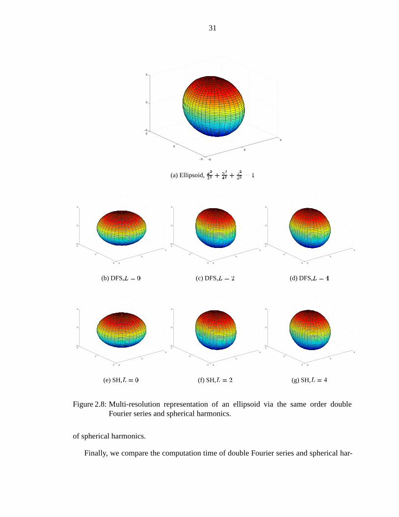
Figure 2.8 and Figure 2.9 show multi-resolution representations of the ellipsoid and

the metasphere, separately. We can see that when spherical harmonics model and the dou-

ble Fourier series model use same number of coefficients, the difference between these

models is very small. A numerical comparison of modeling accuracy is plotted in Figure

2.10. For the regular ellipsoidal shape, truncated spherical harmonics and double Fourier

series show exactly the same rate of convergence in their order. Note that double Fourier

series has a small advantage in accuracy for the regular ellipsoid. For the metasphere,

which contains higher spatial frequencies, double Fourier series also has a faster conver-

gent rate and better accuracy. Here the SVD method was used to compute the coefficients

31

−5

0

5

−5

0

5−5

0

5

(a) Ellipsoid,x2

32+ y2

42+ z2

52= 1

−5

0

5

−5

0

5−5

0

5

(b) DFS,L = 0

−5

0

5

−5

0

5−5

0

5

(c) DFS,L = 2

−5

0

5

−5

0

5−5

0

5

(d) DFS,L = 4

−5

0

5

−5

0

5−5

0

5

(e) SH,L = 0

−5

0

5

−5

0

5−5

0

5

(f) SH,L = 2

−5

0

5

−5

0

5−5

0

5

(g) SH,L = 4

Figure 2.8: Multi-resolution representation of an ellipsoid via the same order doubleFourier series and spherical harmonics.

of spherical harmonics.

Finally, we compare the computation time of double Fourier series and spherical har-

32

−3−2

−10

12

3

−3

−2

−1

0

1

2

3−3

−2

−1

0

1

2

3

(a) Metasphere,ax = 2, ay = 2, az = 2;bx =0:5, by = 0:5, bz = 0; mx = 4, my = 3, mz =2;nx = 2, ny = 3, nz = 4

−3−2

−10

12

3

−3

−2

−1

0

1

2

3−3

−2

−1

0

1

2

3

(b) DFS,L = 0

−3−2

−10

12

3

−3

−2

−1

0

1

2

3−3

−2

−1

0

1

2

3

(c) DFS,L = 4

−3−2

−10

12

3

−3

−2

−1

0

1

2

3−3

−2

−1

0

1

2

3

(d) DFS,L = 8

−3−2

−10

12

3

−3

−2

−1

0

1

2

3−3

−2

−1

0

1

2

3

(e) SH,L = 0

−3−2

−10

12

3

−3

−2

−1

0

1

2

3−3

−2

−1

0

1

2

3

(f) SH,L = 4

−3−2

−10

12

3

−3

−2

−1

0

1

2

3−3

−2

−1

0

1

2

3

(g) SH,L = 8

Figure 2.9: Multi-resolution representation of a metasphere via the same order doubleFourier series and spherical harmonics.

33

0 2 4 6 8 10 12 1410

−6

10−5

10−4

10−3

10−2

10−1

100

Highest Order of Basis Functions: K

Res

idua

l Err

or

DFSSH

(a) Ellipsoid

0 2 4 6 8 10 12 1410

−6

10−5

10−4

10−3

10−2

10−1

100

Highest Order of Basis Functions: K

Res

idua

l Err

or

DFSSH

(b) Metasphere

Figure 2.10: Shape modeling error vs. highest order of modeling basis.

5 10 15 20 25 30 35 4010

−2

10−1

100

101

Highest Order of Basis Functions: K

CP

U ti

me

(sec

ond)

DFSSH

Figure 2.11: CPU time comparison for the computation of double Fourier series and spher-ical harmonics coefficients.

monics coefficients. Figure 2.11 plots the CPU time consumed by computing double

Fourier series and spherical harmonics coefficients. It shows that when the basis func-

tions used by these methods have the same highest order ofK, the CPU time of comput-

ing spherical harmonics coefficients is about2:5 times greater than that of by computing

double Fourier series. In this experiment, the FFT algorithm was used to compute the

34

spherical harmonic coefficients.

2.3 Statistical Shape Modeling

We discuss random field models for statistical shape modeling in this section. The

rest of this section is organized as follows: First, a few important definitions of random

fields are given in Section 2.3.1. In Section 2.3.2, we show that radial functions of ran-

domly oriented polar objects are isotropic random fields over the unit sphere and propose

a procedure to test the hypothesis that a sampled data set over the unit sphere is isotropic.

In Section 2.3.3, the spectral theorem that spherical harmonics comprise the orthogonal

representation of isotropic random field over the unit sphere is proved. Yadrenko gave an

outline of this theorem’s proof in [110]. However, he did not provide the proof of Funk-

Hecke theorem which is a key to proving the spectral theorem. Funk-Hecke theorem was

originally proved and published in 1916 [46] and 1918 [56] by Funk and Hecke in Ger-

man. The proof of Funk-Hecke theorem is not widely available. Thus for completeness,

we provide a detailed proof of the spectral theorem and Funk-Hecke theorem. A brief

discussion of how to corporate the random field model with statistical shape modeling will

end this section. It will be shown in Chapter IV that the statistical uncorrelation of the

shape parameters can be applied to optimal shape filtering and object registration.

2.3.1 Random Field on Unit Sphere

Random fields are stochastic processes whose arguments vary continuously over some

subset ofIRn, n-dimensional Euclidean space. They can be strictly defined on a measure

space(;F ; P ), where is a set with generic element!, F is a�-algebra of subsets of

, andP is a probability measure onF satisfying the following axioms [1]:

(1) 0 � P (A) � 1 andP () = 1;

(2) P (A [ B) = P (A) + P (B), if A \B = ;,A;B 2 F and; is the empty set.

35

The radial functions of 3-D polar objects are examples of random fields inS2 � IR3.

Definition 1 ([57]) A second order random field overS2 � IR3 is a functionZ : S2 !L2(;F ; P ).

A second order random field has been specified overS2 if a random variableZ(x) has

been specified for eachx 2 S2, with EfjZ(x)j2g < 1. We can say that a second order

random field overS is a familyfZ(x); x 2 S2g of square integrable random variables.

A random fieldZ(x) is wide-sense stationary(or wide-sense homogeneous) if it satis-

fies the following conditions:

(1)EfZ(x)g = m, wherem is constant;

(2)Ef(Z(s)�m)(Z(t)�m)�g is a function of(s� t) only.

A wide-sense stationary random field is calledisotropicif

R(jjs� tjj) = Ef(Z(s)�m)(Z(t)�m)�g:

The correlation function of an isotropic random field depends only on the distance be-

tweens andt. The correlation function of such a random field can be thought as invariant

to any rotation around the origin. LetSO(3) denote the group of rotations inIR3 around

the origin. An isotropic random field can also be defined as satisfying

Ef(Z(s)�m)(Z(t)�m)�g = Ef(gZ(s)�m)(gZ(t)�m)�g

whereg 2 SO(3).

Let x1; x2; : : : be a sequence of points andx� be a fixed point inIR3 for which jjxk �x�jj ! 0 ask !1. Then if

jjZ(xk)� Z(x�)jj ! 0 ask!1

we sayZ is continuous in mean squareatx�.

36

Theorem 2 ([1]) A random fieldZ(x) is continuous in mean square at the pointx� 2 IR3

iff its correlation functionR(s; t) is continuous at the points = t = x�.

Theorem 3 (Mercer Theorem [114]) LetR(s; t) be a continuous and non-negative defi-

nite function on the compact intervalT�T � IR2n, with eigenvalues�j and eigenfunctions

�j satisfying ZT

R(s; t)�(t)dt = ��(s) for s 2 T (2.24)

and ZT

�i(t)�j(t)dt = Æij: (2.25)

Then

R(s; t) =1Xj=1

�j�j(s)��j(t) (2.26)

where the series converges absolutely and uniformly onT � T .

2.3.2 Isotropic Random Field onS2

Let (�1; �1) and(�2; �2) denote two directions separated by the angle in the spherical

coordinate system, as shown in Figure 2.12. These angles satisfy the following trigono-

metric identity [3],

cos = cos �1 cos �2 + sin �1 sin �2 cos(�1 � �2): (2.27)

The valuecos is called theangular distancebetween the two directions(�1; �1) and

(�2; �2).

Definition 2 ([110]) A random fieldX(�; �) on the unit sphereS2 is called isotropic in

the wide sense if its mean is constant

EfX(�; �)g = constant (2.28)

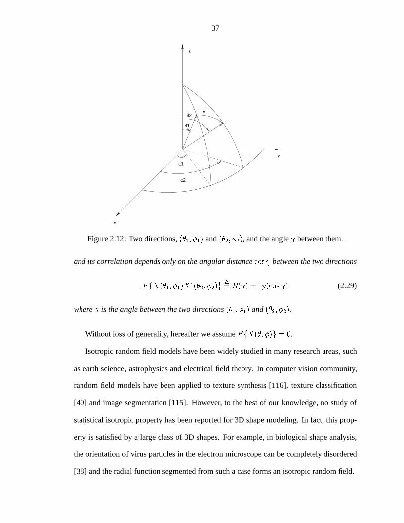
37

φ2

φ1

γ

x

y

z

θ1

θ2

Figure 2.12: Two directions,(�1; �1) and(�2; �2), and the angle between them.

and its correlation depends only on the angular distancecos between the two directions

EfX(�1; �1)X�(�2; �2)g �

= R( ) = (cos ) (2.29)

where is the angle between the two directions(�1; �1) and(�2; �2).

Without loss of generality, hereafter we assumeEfX(�; �)g = 0.

Isotropic random field models have been widely studied in many research areas, such

as earth science, astrophysics and electrical field theory. In computer vision community,

random field models have been applied to texture synthesis [116], texture classification

[40] and image segmentation [115]. However, to the best of our knowledge, no study of

statistical isotropic property has been reported for 3D shape modeling. In fact, this prop-

erty is satisfied by a large class of 3D shapes. For example, in biological shape analysis,

the orientation of virus particles in the electron microscope can be completely disordered

[38] and the radial function segmented from such a case forms an isotropic random field.

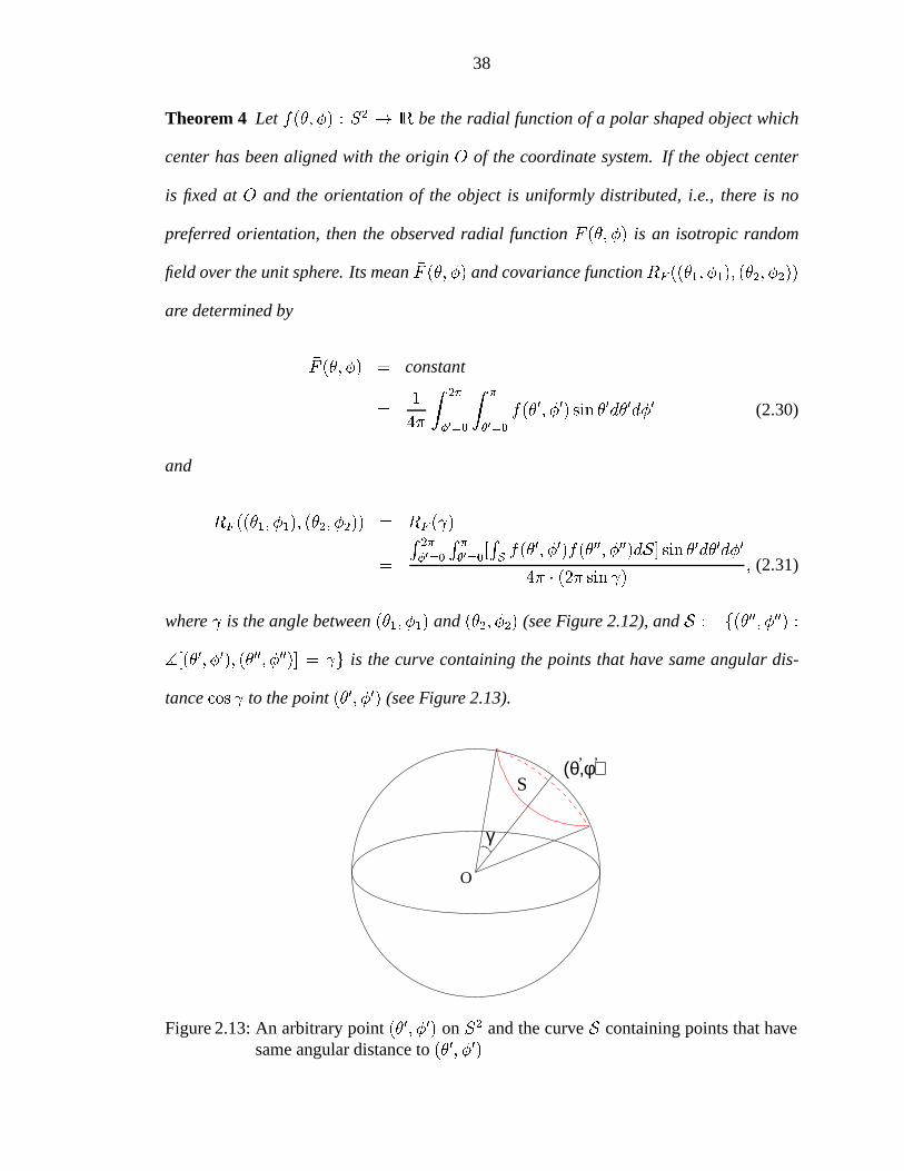
38

Theorem 4 Let f(�; �) : S2 ! IR be the radial function of a polar shaped object which

center has been aligned with the originO of the coordinate system. If the object center

is fixed atO and the orientation of the object is uniformly distributed, i.e., there is no

preferred orientation, then the observed radial functionF (�; �) is an isotropic random

field over the unit sphere. Its mean�F (�; �) and covariance functionRF ((�1; �1); (�2; �2))

are determined by

�F (�; �) = constant

=1

4�

Z 2�

�0=0

Z �

�0=0

f(�0; �0) sin �0d�0d�0 (2.30)

and

RF ((�1; �1); (�2; �2)) = RF ( )

=

R 2�

�0=0

R ��0=0

[RS f(�

0; �0)f(�00; �00)dS] sin �0d�0d�04� � (2� sin ) ; (2.31)

where is the angle between(�1; �1) and(�2; �2) (see Figure 2.12), andS := f(�00; �00) :][(�0; �0); (�00; �00)] = g is the curve containing the points that have same angular dis-

tancecos to the point(�0; �0) (see Figure 2.13).

γ

S

,,(θ,φ)

O

Figure 2.13: An arbitrary point(�0; �0) onS2 and the curveS containing points that havesame angular distance to(�0; �0)

39

Proof:

Let g be a random rotation operator inSO(3) which has uniform distribution over

SO(3). The observed radial functionF can be expressed as

F (�; �) = gf(�; �) = f(�0; �0): (2.32)

Sinceg is uniformly distributed inSO(3), (�0; �0) is uniformly distributed overS2. There-

fore,

E[F (�; �)] = E[f(�0; �0)] =1

4�

Z 2�

�0=0

Z �

�0=0

f(�0; �0) sin �0d�0d�0 (2.33)

This yields equation (2.30). For the correlation functionRF ,

RF ((�1; �1); (�2; �2)) = E[F (�1; �1)F (�2; �2)]

= E[gf(�1; �1)gf(�2; �2)] (2.34)

= E[f(�0; �0)f(�00; �00)]:

The uniform distribution ofg again, makes(�0; �0) have a uniform distribution overS2.

Due to the rigidity of the object,(�00; �00) must be in a fixed angular distance to(�0; �0).

This relation causes(�00; �00) to be uniformly distributed over a curveS that has an angular

distancecos to the point(�0; �0). The length ofS is 2� sin . Therefore equation (2.31)

gives the proper correlation function ofF .

End of proof.

To design an optimal test for the isotropic hypothesis, we need to compute the like-

lihood function of the random field under isotropic and non-isotropic assumption. Let

F (x) be a real-value random field overS2 that is a combination of signals(x) and a white

Gaussian noise fieldn(x), i.e. F (x) = s(x) + n(x), x 2 S2. The correlation function

of F is defined asRF (x; y) = E[F (x)F (y)]. Let F = [F1F2 � � �FN ]T be the random

vector obtained through samplingF atx = [x1x2 � � �xN ]T , xi 2 S2, i.e.,Fi , F (xi), the

correlation functionR can be estimated from the covariance matrixRF = E[FFT ].

40

If we assume the random fields(x) is isotropic, the correlation function ofF will be

in the form ofRF (x; y) = RF (kx � yk) = Rs(kx � yk) + Æ(x � y) � �2n, where�2n is

the variance of the noise field. We propose a sub-optimal isotropic test of how close the

estimated correlation function is to the form ofRF (kx� yk) and classify the random field

into isotropic or non-isotropic categories accordingly:

1. Compute covariance matrixRF

2. EstimateRs(d) (d 2 [0; �]), the correlation function ofs(x). It is determined by

Rs = argminP

i;j kRF ij � Rs(](xi; xj))k2.

3. Let e =P

i;j kRF ij � Rs(](xi; xj))k2. If e > threshold,F is non-isotropic, oth-

erwise,F is isotropic. The threshold is determined by the variance of noise�n and

the sampling statistics of the estimatorRs.

2.3.3 Orthogonal Representation of Isotropic Random Field onS2

Theorem 5 ([110]) A mean-square continuous homogeneous isotropic random fieldX(�; �)

of zero mean inS2 can be represented as:

X(�; �) =1Xl=0

lXm=�l

A(l; m)Y ml (�; �) (2.35)

with Y ml (�; �) denoting the spherical harmonics of degreel and orderm, and

A(l; m) =

Z 2�

0

Z �

0

X(�; �)Y m�l (�; �)d�;� (2.36)

such that

EfA(l; m)g = 0 (2.37)

and

EfA(l; m)A�(l0

; m0

)g = �l Æl;l0 Æm;m0 (2.38)

41

where

�l = 2�

Z 1

�1

(t)Pl(t) dt (2.39)

is the coefficient in the Legendre series of the correlation function, and (cos ) = R( )

is the correlation function ofX(�; �).

Proof:

By Theorem 2 in Section 2.3.1, we know that the correlation functionR( ) of the

mean-square continuous homogeneous isotropic random fieldX(�; �) onS2 is continuous

on [�1; 1]. By Funk-Hecke theorem, we haveZS2 (cos )Y m

l (�2; �2) d�2;�2 = �lYml (�1; �1) (2.40)

which means the setf�l; Y ml (�; �)g is a complete set of eigenvalues and orthonormal

eigenvectors for the correlation functionR( ). By Mercer theorem [114], the following

expansion holds for all(�1; �1) and(�2; �2):

(cos ) =1Xl=0

lXm=�l

�l Yml (�1; �1)Y

m�l (�2; �2): (2.41)

This expansion converges absolutely and uniformly [114].

Notice

EfX(�; �)A�(l0

; m0

)g

= EfX(�; �)

ZS2X�(�2; �2)Y

m0

l0(�2; �2)d�2;�2g

=

ZS2EfX(�; �)X�(�2; �2)Y m

0

l0(�2; �2)d�2;�2g

=

ZS2 (cos )Y m

0

l0(�2; �2)d�2;�2

= �l0Ym0

l0(�; �)

42

where the fact (2.40) is used to reach the last step. So, we have

EfA(l; m)A�(l0

; m0

)g = EfZS2X(�; �)Y m�

l (�; �)d�;�A�(l

0

; m0

)g

=

ZS2EfX(�; �)A�(l

0

; m0

)gY m�l (�; �)d�;�

=

ZS2�l0Y

m0

l0(�; �)Y m�

l (�; �)d�;�

= �lÆl;l0Æm;m0

which is (2.38).

Let XL(�; �) =PL

l=0

Plm=�l A(l; m)Y m

l (�; �). We need to show that

limL!1

EfjX(�; �)� XL(�; �)j2g = 0: (2.42)

Note

EfjX(�; �)� XL(�; �)j2g

= EfX(�; �)(X�(�; �)g � EfX(�; �)X�L(�; �)g

�EfXL(�; �)(X�(�; �)g+ EfXL(�; �)X

�L(�; �))g

= (cos )j =0 �LXl=0

lXm=�l

EfX(�; �)A�(l; m)gY m�l (�; �)�

LXl=0

lXm=�l

EfA(l; m)X�(�; �)gY ml (�; �) +

LXl=0

lXm=�l

LXl0=0

l0Xm0=�l0

EfA(l; m)A�(l0; m0)gY ml (�; �)Y m0�

l0 (�; �)

= (cos )j =0 �LXl=0

lXm=�l

�l Yml (�; �)Y m�

l (�; �) (2.43)

By (2.41), the limit of the above equation equals0 whenL!1.

End of proof.

Theorem 6 (Funk-Hecke Theorem)Let (v) be a continuous function on[�1; 1]. Let

Y ml (�2; �2) be any surface spherical harmonic of degreel and orderm. Then for any unit

43

vector(�1; �1) 2 S2, we haveZS2 (cos )Y m

l (�2; �2) d�2;�2 = �lYml (�1; �1) (2.44)

where is the angular distance (2.27) between(�1; �1) and(�2; �2), d�2;�2 = sin �2 d�2 d�2,

and

�l = 2�

Z 1

�1

(t)Pl(t)dt (2.45)

with Pl(x) denoting the Legendre polynomial1 of degreel.

Proof2:

The Legendre polynomials are orthogonal and constitute a complete set of functions

on the interval[�1; 1]. By the Sturm-Liouville Theory [3, 59], any function (x) contin-

uous on[�1; 1] can be written as its Legendre series, which converges uniformly. More

precisely, we have

(x) =1Xk=0

akPk(x) (2.46)

whereP1

k=0 akPk(x) is Legendre series3 of the function (x), and

ak =2k + 1

2

Z 1

�1

(x)Pk(x)dx: (2.47)

We also have

limn!1

Z 1

�1

" (x)�

nXk=0

akPk(x)

#2dx = 0: (2.48)

By the Holder’s inequality, we have�����ZS2

" (cos )�

nXk=0

akPk(cos )

#Y ml (�2; �2) d�2;�2

�����2

�ZS2

" (cos )�

nXk=0

akPk(cos )

#2d�2;�2

ZS2Y ml (�2; �2)Y

m�l (�2; �2) d�2;�2 : (2.49)

1The Legendre polynomialPl(x) is defined in Appendix A.2.2This proof is included for completeness.3In fact, the equation (2.46) holds if

R1

�1j (x)j2dx <1 [59].

44

SinceZS2

" (cos )�

nXk=0

akPk(cos )

#2d�2;�2 = 2�

Z 1

�1

" (x)�

nXk=0

akPk(x)

#2dx

(2.50)

and ZS2Y ml (�2; �2)Y

m�l (�2; �2) d�2;�2 = 1; (2.51)

the inequality in (2.49) can be written as�����ZS2

" (cos )�

nXk=0

akPk(cos )

#Y ml (�2; �2) d�2;�2

�����2

�

4�2Z 1

�1

" (x)�

nXk=0

akPk(x)

#2dx: (2.52)

Taking limit to both sides of this inequality and using ( 2.48), we have

limn!1

�����ZS2

" (cos )�

nXk=0

akPk(cos )

#Y ml (�2; �2) d�2;�2

�����2

= 0 (2.53)

which means

limn!1

ZS2

" (cos )�

nXk=0

akPk(cos )

#Y ml (�2; �2) d�2;�2 = 0: (2.54)

i.e.,ZS2 (cos )Y m

l (�2; �2) d�2;�2 = limn!1

nXk=0

ak

ZS2Pk(cos )Y

ml (�2; �2) d�2;�2 : (2.55)

By Addition Theorem for spherical harmonics (Appendix A.1.3),Pl(cos ) can be written

as

Pl(cos ) =4�

2l + 1

lXm=�l

Y ml (�1; �1)Y

m�l (�2; �2): (2.56)

Using the orthogonality of the spherical harmonics, we haveZS2Pk(cos )Y

ml (�2; �2) d�2;�2 =

4�

2l + 1Æk;lY

ml (�1; �1): (2.57)

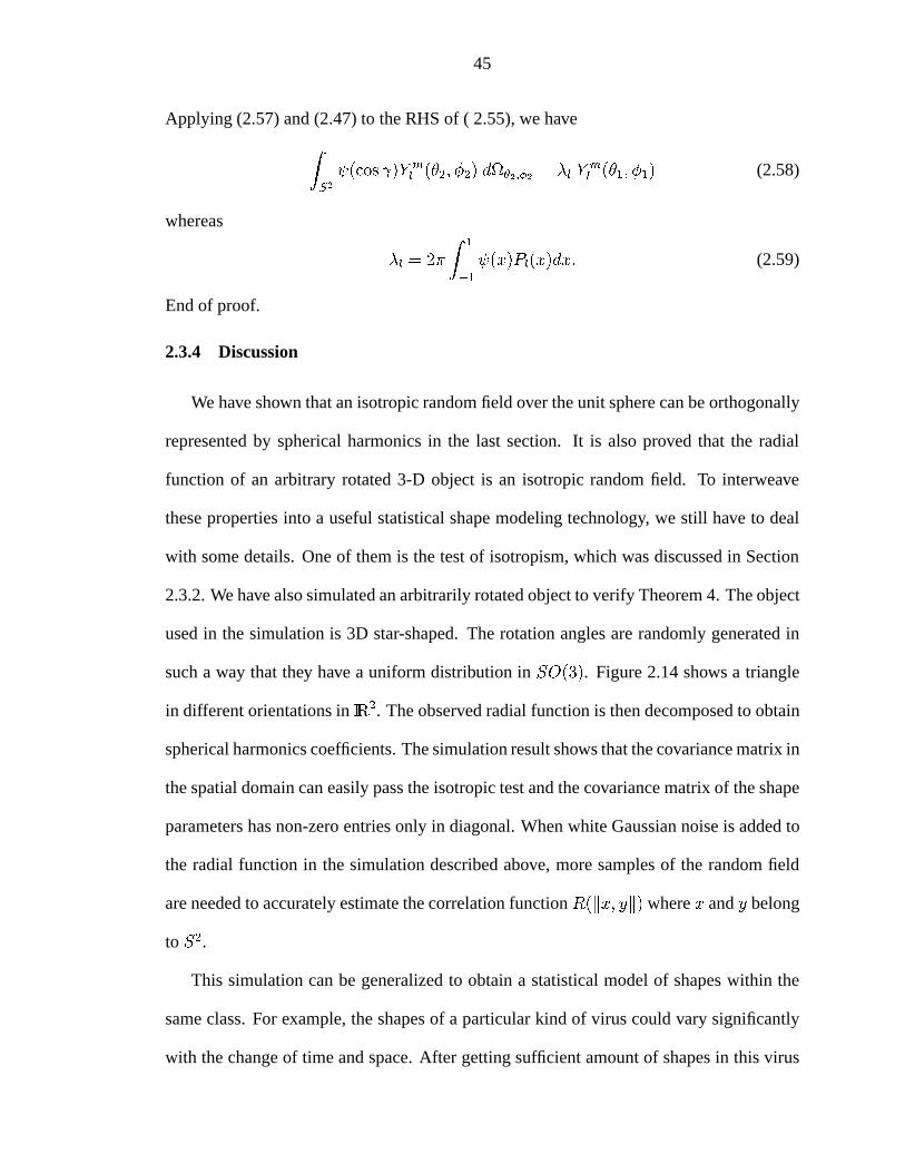
45

Applying (2.57) and (2.47) to the RHS of ( 2.55), we haveZS2 (cos )Y m

l (�2; �2) d�2;�2 = �l Yml (�1; �1) (2.58)

whereas

�l = 2�

Z 1

�1

(x)Pl(x)dx: (2.59)

End of proof.

2.3.4 Discussion

We have shown that an isotropic random field over the unit sphere can be orthogonally

represented by spherical harmonics in the last section. It is also proved that the radial

function of an arbitrary rotated 3-D object is an isotropic random field. To interweave

these properties into a useful statistical shape modeling technology, we still have to deal

with some details. One of them is the test of isotropism, which was discussed in Section

2.3.2. We have also simulated an arbitrarily rotated object to verify Theorem 4. The object

used in the simulation is 3D star-shaped. The rotation angles are randomly generated in

such a way that they have a uniform distribution inSO(3). Figure 2.14 shows a triangle

in different orientations inIR2. The observed radial function is then decomposed to obtain

spherical harmonics coefficients. The simulation result shows that the covariance matrix in

the spatial domain can easily pass the isotropic test and the covariance matrix of the shape

parameters has non-zero entries only in diagonal. When white Gaussian noise is added to

the radial function in the simulation described above, more samples of the random field

are needed to accurately estimate the correlation functionR(kx; yk) wherex andy belong

to S2.

This simulation can be generalized to obtain a statistical model of shapes within the

same class. For example, the shapes of a particular kind of virus could vary significantly

with the change of time and space. After getting sufficient amount of shapes in this virus

46

Figure 2.14: A triangle with random orientations inIR2.

class, these shapes can be used as a training set to extract the covariance matrix of the ran-

dom field shape model. If this covariance matrix passes the isotropic test, the isotropic ran-

dom field model can then be regarded as a statistical shape model of this class of viruses.

Our random field model of 3D shapes is different from other statistical shape modeling

technologies in the following two aspects: First, it integrates the global shape variations

into a single correlation function of the isotropic random field. The isotropism is primarily

caused by arbitrary rotations of the object. But other reasons, such as shape variations,

are not banned. As we stated in the introduction, the published statistical shape model-

ing technologies usually only compute the covariance matrices of shape parameters and

have contributed very little effort to generating correlation function in the spatial domain

due to the complicated expression and high computational complexities; Second, in the

frequency domain, the random shape parameters in our model are uncorrelated. This

property is important in shape filtering. Other statistical shape models usually achieves

this uncorrelation through principle component analysis. This PCA step is not necessary

for our shape models.

CHAPTER III

CENTER ESTIMATION

3.1 Introduction

We depicted the statistic polar shape modeling techniques in Chapter II. These meth-

ods highly depend on the object position relative to the origin and coordinate axes. A

proper choice of origin and coordinate axes is important to use shape modeling basis func-

tions efficiently and to estimate the shape parameters accurately. For different assumptions

and objectives, the optimum center for shape representation may be different. For exam-

ple, Piramuthu pointed out that to maximize the average confidence in shape estimation,

the optimum center may not coincide with the object centroid [87]. It was also conjectured

that the optimum center may be the center for which the minimum radius of boundary is

maximized [87]. However, to simplify the computation, the object centroid is a natural

choice as the center for shape representation. This choice has been verified to be reliable

in most practical cases [76, 92].

When an object has symmetry relative to a center, its centroid coincides with the object

symmetric center. Aligning the origin with the object symmetric center is an optimum

choice because the basis functions in many shape modelings are defined to be symmetric

to the origin. For the shape modeling of a specific object, if the origin is not properly

chosen, e.g., to be too close to the object boundary or even outside the object, the resulted

47

48

shape representation can be very inefficient, because it can not take advantage of any

object symmetry and may have to contain high spatial frequencies that do not exist if the

optimum center is in use. The following example illustrates how center estimation error

can deteriorate the efficiency of shape modeling.

A solid sphere is contained in a three dimensional image and coarsely segmented to

obtain the boundary of this sphere. We want to use spherical harmonics to model this

shape. Since a sphere is the object with the most symmetry, aligning the origin with its

symmetric center which is also its centroid is certainly the appropriate method. This can be

verified by the property of the first degree spherical harmonics function which is a sphere

of radiusp4�. If the object center and the origin are perfectly aligned, one parameter will

be sufficient to describe the entire object. However, the error in center estimation can make

it very difficult to use the symmetry of the sphere. Table 3.1 and Figure 3.1 show how

the efficiency and accuracy of shape representation decrease with the increasing center

estimation error. The first column in Table 3.1 lists the amount of center shift, which can

Table 3.1: Shape modeling error vs. center shift for unit sphereCenter Spherical Harmonics DegreeShift L = 0 L = 2 L = 4 L = 6 L = 8 L = 10e = 0 0 0 0 0 0 0e = 0:2r 5.04e-2 9.19e-7 1.15e-9 1.81e-12 3.87e-15 2.19e-15e = 0:4r 1.03e-1 1.48e-5 7.57e-8 4.86e-10 3.51e-12 2.74e-14e = 0:6r 1.61e-1 7.75e-5 9.33e-7 1.41e-8 2.36e-10 4.23e-12e = 0:8r 2.26e-1 2.63e-4 6.01e-6 1.66e-7 5.05e-9 1.62e-10

be caused by inaccurate center estimation. The center shift is normalized with respect

to the radius of the sphere. The parameterL is the highest order of spherical harmonics

used in modeling. This table shows that when the center shift is increasing, we need more

and more spherical harmonics basis functions to get an accurate shape representation of

the unit sphere. When the estimated center is shifted by0:8r, we need to useL = 10

49

0 2 4 6 8 10 12 1410

−15

10−10

10−5

100

Highest Order of Spherical Harmonics in Shape Modeling: L

Res

idua

l Err

or

center shift = 0.2 radiuscenter shift = 0.4 radiuscenter shift = 0.6 radiuscenter shift = 0.8 radius

Figure 3.1: Shape modeling error vs. center shift for unit sphere

components in the spherical harmonic expansion in order to approximate a sphere with

the error magnitude in the order of10�10. Furthermore, the computational complexity for

L = 10 is much higher than that forL = 0, with which we can exactly represent a centered

sphere.

The above example shows the importance of aligning the origin with the center of the

object. However, unless the measurement system defines a natural geometry of the object,

the true center of the object is not well defined. Furthermore, if the surface sample data

is obtained through segmentation, the segmentation noise makes it impossible to find the

true center of the object. Given a set of surface sample data, the following two methods

are often used to estimate the center of the object [76]:

➀ Assuming that the sample data is evenly distributed over the surface of the object,

the center of gravity of the sample data should provide a good estimate for the center.

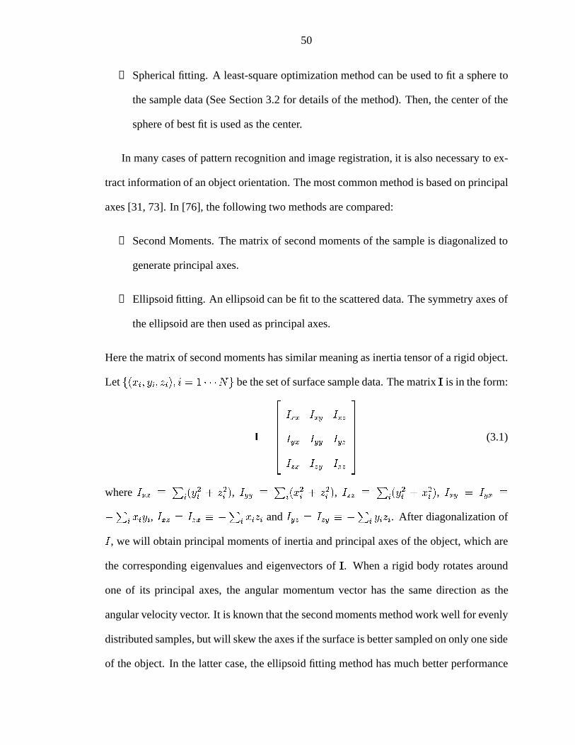
50

➁ Spherical fitting. A least-square optimization method can be used to fit a sphere to

the sample data (See Section 3.2 for details of the method). Then, the center of the

sphere of best fit is used as the center.

In many cases of pattern recognition and image registration, it is also necessary to ex-

tract information of an object orientation. The most common method is based on principal

axes [31, 73]. In [76], the following two methods are compared:

➀ Second Moments. The matrix of second moments of the sample is diagonalized to

generate principal axes.

➁ Ellipsoid fitting. An ellipsoid can be fit to the scattered data. The symmetry axes of

the ellipsoid are then used as principal axes.

Here the matrix of second moments has similar meaning as inertia tensor of a rigid object.

Let f(xi; yi; zi); i = 1 � � �Ng be the set of surface sample data. The matrixI is in the form:

I =

2666664Ixx Ixy Ixz

Iyx Iyy Iyz

Izx Izy Izz

3777775 (3.1)

whereIxx � Pi(y

2i + z2i ), Iyy �

Pi(x

2i + z2i ), Izz �

Pi(y

2i + x2i ), Ixy = Iyx �

�Pi xiyi, Ixz = Izx � �Pi xizi andIyz = Izy � �Pi yizi. After diagonalization of

I, we will obtain principal moments of inertia and principal axes of the object, which are

the corresponding eigenvalues and eigenvectors ofI. When a rigid body rotates around

one of its principal axes, the angular momentum vector has the same direction as the

angular velocity vector. It is known that the second moments method work well for evenly

distributed samples, but will skew the axes if the surface is better sampled on only one side

of the object. In the latter case, the ellipsoid fitting method has much better performance

51

[76]. However, it is also observed that some samples may yield other types of quadratic

surface, instead of an ellipsoidal surface. For those rare cases, the more robust method of

moments must be used.

In this study, we use the method of ellipsoid fitting because it can jointly estimate the

centroid and principal axes of 3D objects. The rest of this chapter shows how this method

works. A lower bound is derived for center estimation by ellipsoid fitting and compared

with the simulation results.

3.2 Ellipsoid Fitting

This section studies the reconstruction of a three dimensional ellipsoid from scattered

surface sample data. The ellipse and ellipsoid are often used in the fields of medical

imaging and computer vision to model object shapes. In medical imaging, the coronary

arteries may be represented and visualized efficiently by a generalized cylinder model with

elliptical cross-sections [44, 64], and the shape or volume of anatomical organs such as

heart and spine can be modeled as ellipsoids [7, 16]. In computer vision, simple patterns,

such as ellipses, are important to recognize and position curved three-dimensional objects

from image contours [58, 70, 106, 113].

As we discussed in the introduction, the ellipsoid fitting method is preferred when

the sample data is not evenly distributed over the surface. We adopt this method because

the object center and principal axes can be jointly estimated straightforwardly, so that the

origin and axes of shape modeling coordinate system can be aligned with them.

The ellipsoid is a special case of quadratic surface which has a general expression as:

f(x; y; z) : Ax2 +By2 + Cz2 +Dxy + Exz + Fyz +Gx +Hy + Iz + J = 0g (3.2)

where(x; y; z) are the coordinates of the point on the ellipsoid surface,(A;B;C; :::; J) are

the parameters which describe the location, size and orientation of the ellipsoid. There are

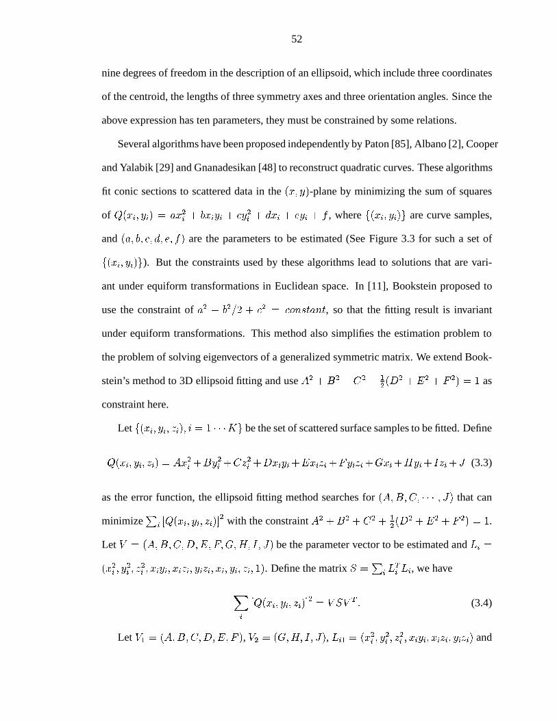
52

nine degrees of freedom in the description of an ellipsoid, which include three coordinates

of the centroid, the lengths of three symmetry axes and three orientation angles. Since the

above expression has ten parameters, they must be constrained by some relations.

Several algorithms have been proposed independently by Paton [85], Albano [2], Cooper

and Yalabik [29] and Gnanadesikan [48] to reconstruct quadratic curves. These algorithms

fit conic sections to scattered data in the(x; y)-plane by minimizing the sum of squares

of Q(xi; yi) = ax2i + bxiyi + cy2i + dxi + eyi + f , wheref(xi; yi)g are curve samples,

and (a; b; c; d; e; f) are the parameters to be estimated (See Figure 3.3 for such a set of

f(xi; yi)g). But the constraints used by these algorithms lead to solutions that are vari-

ant under equiform transformations in Euclidean space. In [11], Bookstein proposed to

use the constraint ofa2 + b2=2 + c2 = constant, so that the fitting result is invariant

under equiform transformations. This method also simplifies the estimation problem to

the problem of solving eigenvectors of a generalized symmetric matrix. We extend Book-

stein’s method to 3D ellipsoid fitting and useA2 + B2 + C2 + 12(D2 + E2 + F 2) = 1 as

constraint here.

Let f(xi; yi; zi); i = 1 � � �Kg be the set of scattered surface samples to be fitted. Define

Q(xi; yi; zi) = Ax2i +By2i +Cz

2i +Dxiyi+Exizi+Fyizi+Gxi+Hyi+ Izi+J (3.3)

as the error function, the ellipsoid fitting method searches for(A;B;C; � � � ; J) that can

minimizeP

i [Q(xi; yi; zi)]2 with the constraintA2 + B2 + C2 + 1

2(D2 + E2 + F 2) = 1.

Let V = (A;B;C;D;E; F;G;H; I; J) be the parameter vector to be estimated andLi =

(x2i ; y2i ; z

2i ; xiyi; xizi; yizi; xi; yi; zi; 1). Define the matrixS =

Pi L

Ti Li, we have

Xi

[Q(xi; yi; zi)]2 = V SV T : (3.4)

Let V1 = (A;B;C;D;E; F ), V2 = (G;H; I; J), Li1 = (x2i ; y2i ; z

2i ; xiyi; xizi; yizi) and

53

Li2 = (xi; yi; zi; 1). The matrixS can be written as

S =

264 S11 S12

S21 S22

375 (3.5)

whereS11 =P

i LTi1Li1, S12 =

Pi L

Ti1Li2, S21 =

Pi L

Ti2Li1, andS22 =

Pi L

Ti2Li2.

Substitution of (3.5) into (3.4) yields

V SV T = (V1;V2)

264 S11 S12

S21 S22

375264 V T

1

V T2

375 = V1S11VT1 + 2V1S12V

T2 + V2S22V

T2 :

To minimizeV SV T , we let the derivatived(V SVT )

d(V2)to be zero, i.e.,

d(V SV T )

d(V2)= 2V1S12 + 2V2S22 = 0:

This leads to

V2 = �V1S12S�122 : (3.6)

SubstitutingV2 = �V1S12S�122 into V SV T , we have

V SV T = V1(S11 � S12S�122 S21)V

T1 = V1(eS)V T

1 (3.7)

whereeS = S11 � S12S�122 S21.

Let us defineD1 = diag(1; 1; 1; 12; 12; 12), the constraintA2 + B2 + C2 + 1

2(D2 +

E2 + F 2) = 0 can be described in the formV1D1VT1 = 1. Therefore, the constrained

minimization ofV SV 0 has been converted to minimization ofV1 eSV T1 ��V1D1V

T1 . Taking

the derivative overV1 and setting it to zero, we obtain

2eSV T1 � 2�D1V

T1 = 0: (3.8)

This indicates that the vectorV T1 should be the eigenvector ofeS. In the implementation, the

eigenvector of best geometric fit is chosen to be the final solution of parameter estimation.

The center and principal axes of an ellipsoid are completely determined by the parameter

vectorV .

54

3.3 Lower Bound for Center Estimation by Ellipsoid Fitting

To evaluate the performance of ellipsoid fitting, we develop a lower bound for the

variance of unbiased center estimators under a Gaussian segmentation noise model. It is

also shown that when the segmentation noise level is low and has a Gaussian distribution,

the ellipsoid fitting method studied in section 3.2 is a maximum likelihood estimator of the

ellipsoid parameter vector, and its performance can approach the developed lower bound.

Our derivation of the lower bound follows similar steps as the derivation of a Cram´er-Rao

bound.

The effectiveness of an unbiased estimator can be characterized by its variance. Cram´er-

Rao bound, the inverse of Fisher information matrix, describes the minimum obtainable

mean square error associated with a given estimate of a set of parameters. Letz represent

observed data and� = [�1; �2; � � � ; �n]T be the parameter vector to be estimated fromz.

The Fisher information matrixJ is defined as [91]:

Jij = E

�@ ln p(zj�)

@�i

@ ln p(zj�)@�j

�(3.9)

= �E�@2 ln p(zj�)@�i@�j

�whereJij is (i; j)-entry of then� n matrixJ. Let = J�1. The Cram´er-Rao bound on

the covariance of the estimation error is given by

Eh�i(z)�j(z)

i� ij (3.10)

where�i(z) and �j(z) are the unbiased estimators of�i and�j, andij is (i; j)-entry of

. The derivation of such a bound for the ellipsoid parameter vectorV is described as

follows.

First, let us set up the segmentation noise model. Write equation (3.2) in the spherical

55

coordinate system as:

Ar2(sin � cos�)2 +Br2(sin � sin�)2 + Cr2(cos �)2

+1

2[Dr2(sin2 � sin 2�) + Er2(sin 2� cos�) + Fr2(sin 2� sin�)]

+Gr sin � cos�+Hr sin � sin�+ Ir cos � + J = 0; (3.11)

where(r; �; �) are spherical coordinates of point(x; y; z) on the surface. To arrange equa-

tion (3.11) into a quadratic form ofr, we define

A1 = A(sin � cos�)2 +B(sin � sin�)2 + C(cos �)2 +

1

2[D(sin2 � sin 2�) + E(sin 2� cos�) + F (sin 2� sin�)]

B1 = G sin � cos�+H sin � sin�+ I cos �

C1 = J: (3.12)

Substitute (3.12) into (3.11), we have

A1r2 +B1r + C1 = 0 (3.13)

If we assume the origin of the spherical coordinate system is inside the ellipsoid, the true

radial value in each direction(�; �) is:

r0(�; �) =

pB2

1 � 4A1C1 � B1

2A1: (3.14)

In ellipsoid fitting,P

iQ2(xi; yi; zi) is minimized to estimate the parameter vector. It

is proved in [11] thatQ(xi; yi; zi) = Q(ri; �i; �i) / ( rir0(�i;�i)

)2�1, wherer0 is determined

by (3.14). Therefore the ellipsoid fitting method implements a maximum likelihood esti-

mation of the parameter vector, when it is assumed that the noise in each direction(�i; �i)

is uncorrelated and the segmentation data follows the probability density function

f(ri) = �i � exp[�(

r2ir20;i(�i;�i)

� 1)2

�2]; ri > 0 (3.15)

56

wherer0;i is the true radius in the sample direction(�i; �i) determined by (3.14) and�i is

the normalization factor. Ifri � r0;i � r0;i, we have( r2ir20;i� 1)2 � 4( ri�r0;i

r0;i)2, andf(ri)

can be approximated by

f1(ri) = �i � exp[�4(ri � r0;i�r0;i

)2]; ri > 0 (3.16)

Notice thatf1(ri) is not a probability density function with respect tor 2 (1;1). To

force f1(ri) to become a probability density function, the normalization factor�i has to

modified as

�1;i = 1=

Z 1

�1exp[�4( x

�r0;i)2]dx =

2

r0;i�p�:

This approximation is illustrated in Figure 3.2.

3 3.5 4 4.5 5 5.5 6 6.5 70.08

0.1

0.12

0.14

0.16

0.18

0.2

0.22

r

f(r)

f(r)=α exp(−(r2/r02−1)2)

f1(r)=α exp(−4(r/r

0−1)2)

Figure 3.2: Approximation off(r) by f1(r) under the conditionr� r0 � r0. Herer0 = 5and� = 1.

During the derivation of lower bound and the simulation of the ellipsoid fitting perfor-

mance, we adoptf1(r) as the probability density function of segmentation data. This is

equivalent to a Gaussian noise model. In the following, we derive the Fisher information

for parameterA with the above noise model.

57

Taking the logarithm in both side of (3.16), we have

ln f1(r) = �4(r � r0�r0

)2 + ln�1 = �4(r � r0�r0

)2 � ln r0 � ln(�p�=2): (3.17)

The partial derivative ofln f1(r) with respect toA is

@ ln f1(r)

@A=@ ln f1(r)

@r0� @r0@A1

� @A1

@A: (3.18)

where

@ ln f1(r)

@r0= 8

r(r � r0)

�2r30� 1

r0; (3.19)

@r0@A1

= �( C1

A1

pB2

1 � 4A1C1

+

pB2

1 � 4A1C1 �B1

2A21

); (3.20)

@A1

@A= (sin � cos�)2: (3.21)

The second order partial derivative ofln f1(r) toA is

@2 ln f1(r)

@A2=

@A1

@A� [@ ln f1(r)

@r0� @

2r0@A2

1

� @A1

@A+@r0@A1

� @2 ln f1(r)

@r20� @r0@A1

� @A1

@A]

= (@A1

@A)2 � [(@ ln f1(r)

@r0) � (@

2r0@A2

1

) + (@r0@A1

)2 � @2 ln f1(r)

@r20] (3.22)

where

@2 ln f1(r)

@r20= �24 r2

�2r40+ 16

r

�2r30+

1

r20: (3.23)

The mean of@2 ln f1(r)@A2

is:

E[@2 ln f1(r)

@A2] = �( 8

�2r20+

2

r20)(@r0@A1

)2 � (@A1

@A)2: (3.24)

Let the total number of points in the segmentation data set be denoted asK. With the

assumption that noise are independent over different direction(�i; �i), the joint probability

density function for the set of sample data isQK

i=1 f1(ri), wheref1(ri) is the probability

density function of the segmentation data in direction(�i; �i). Therefore, the Fisher infor-

mation for the parameterA is:

IA =KXi=1

�E[@2 ln f1;i(ri)

@A2]: (3.25)

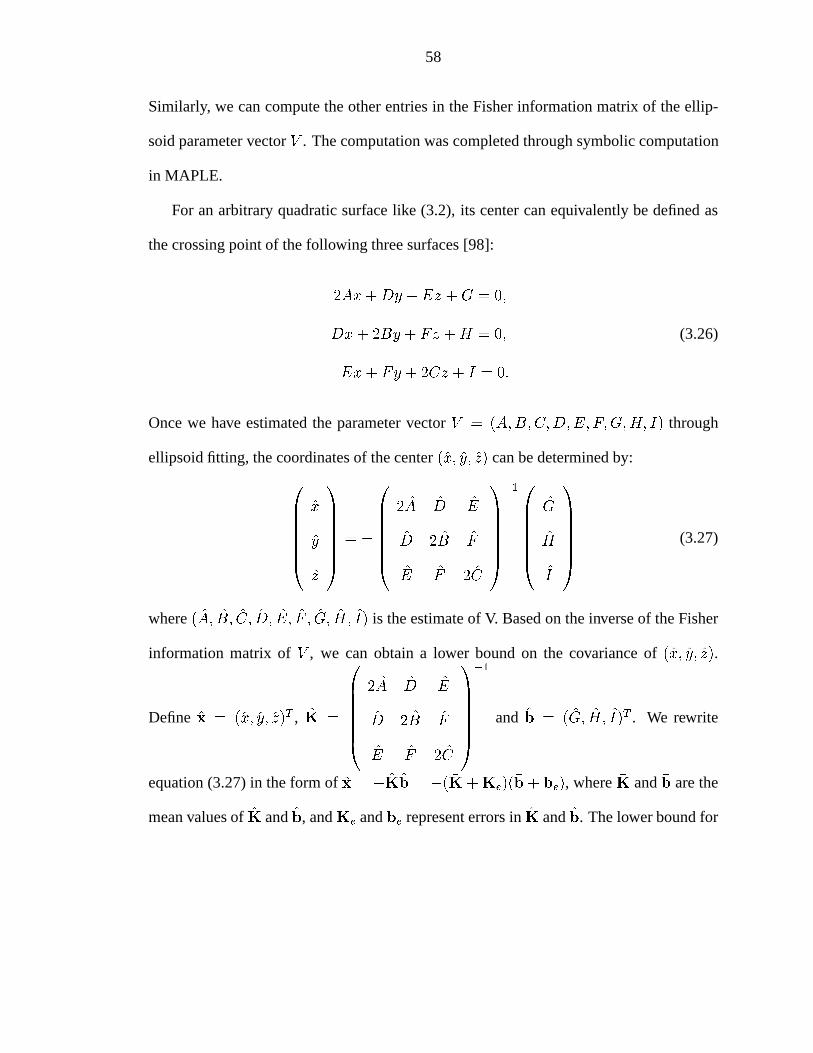
58

Similarly, we can compute the other entries in the Fisher information matrix of the ellip-

soid parameter vectorV . The computation was completed through symbolic computation

in MAPLE.

For an arbitrary quadratic surface like (3.2), its center can equivalently be defined as

the crossing point of the following three surfaces [98]:

2Ax+Dy + Ez +G = 0;

Dx + 2By + Fz +H = 0; (3.26)

Ex + Fy + 2Cz + I = 0:

Once we have estimated the parameter vectorV = (A;B;C;D;E; F;G;H; I) through

ellipsoid fitting, the coordinates of the center(x; y; z) can be determined by:0BBBBB@x

y

z

1CCCCCA = �

0BBBBB@2A D E

D 2B F

E F 2C

1CCCCCA�10BBBBB@

G

H

I

1CCCCCA (3.27)

where(A; B; C; D; E; F ; G; H; I) is the estimate of V. Based on the inverse of the Fisher

information matrix ofV , we can obtain a lower bound on the covariance of(x; y; z).

Define x = (x; y; z)T , K =

0BBBBB@2A D E

D 2B F

E F 2C

1CCCCCA�1

and b = (G; H; I)T . We rewrite

equation (3.27) in the form ofx = �Kb = �( �K +Ke)(�b + be), where�K and�b are the

mean values ofK andb, andKe andbe represent errors inK andb. The lower bound for

59

the covariance of the center estimator can be obtained from following computation:

cov(x) = E�(x� �x)(x� �x)T

�= E

h(Kb� �K�b)(Kb� �K�b)T

i= cov( �Kbe) + cov(Ke

�b) + cov(Kebe)

> cov( �Kbe) + cov(Ke�b)

� �KF�1(b) �KT + cov(Ke�b) (3.28)

whereF�1(b) denotes the inverse of Fisher information matrix of the parameter vector

(G;H; I). In the above derivation, we have assumed that cov(Kebe) is much smaller than

cov( �Kbe) and cov(Ke�b). �KF�1(b) �KT is an approximation of cov( �Kbe). The accuracy

of this approximation improves as var(Kij) ! 0. To further simplify the computation of

lower bound, we let�b equal zero in our experiment so that the term cov(Ke�b) in (3.28)

can be ignored.

3.4 Simulation Results

To evaluate the performance of center estimation by the proposed ellipsoid fitting

method, we have simulated noisy segmentation data sets and applied ellipsoid fitting

method to estimate the object center. In the simulation, segmentation data in each sam-

ple direction(�i; �i) was generated independently with Gaussian distributionf1(ri) =

�i � exp[�4( ri�r0;i�r0;i)2], wherer0;i is the true radial value. Sampling direction(�; �) is

evenly distributed over a grid on[0; �]� [0; 2�). The true surface used in the simulation is

an ellipsoidx2

72+ y2

62+ z2

52= 1. One such simulated segmentation in a 2D cross section of

the ellipsoid is shown in Figure 3.3. We think that these simulated errors are representa-

tive of errors incurred by coarse hand segmentation or automatic segmentation of a noisy

boundary. It is shown in Appendix B that the segmentation error can be modeled by a

60

−8 −6 −4 −2 0 2 4 6 8−8

−6

−4

−2

0

2

4

6

8

x

y

True boundary Segmentation data

Figure 3.3: Segmentation data on a cross section of the ellipsoid,� = 0:2.

Gaussian random variable in 1D edge detection. If we regard the 3D surface segmentation

as implemented through 1D edge detection along each sampling direction and assume that

surface curvature has no significant influence over the detection, our noise model will sim-

ulate the segmentation error very well. However, if the sampling density is relatively high

as compared to the object size, the segmentation noise in neighborhood will be correlated

[72].

For each noise level,200 sets of simulated segmentation data were generated. Figure

3.4(a) shows the bias of the center coordinate estimatorx. Figure 3.4(b) compares the

variance ofx with the developed lower bound. When the noise level is low, the variance

of x is very close to the lower bound. This proves that this center estimator is an efficient

maximum likelihood estimator when the noise level is low. We have also simulated the

segmentation data with� larger than0:5 with the same ellipsoid used above. The results

show that the performances of the ellipsoid fitting center estimator is not stable because of

the outliers in the segmentation data.

61

3.5 Conclusion

We established that the estimator of the ellipsoid parameter vector proposed by Book-

stein is a maximum likelihood estimator when the segmentation noise level is low. A lower

bound has been derived for the variance of center estimator with Gaussian noise model of

the segmentation data. The simulated results show that the center estimator by ellipsoid

fitting method is efficient when the noise level is low.

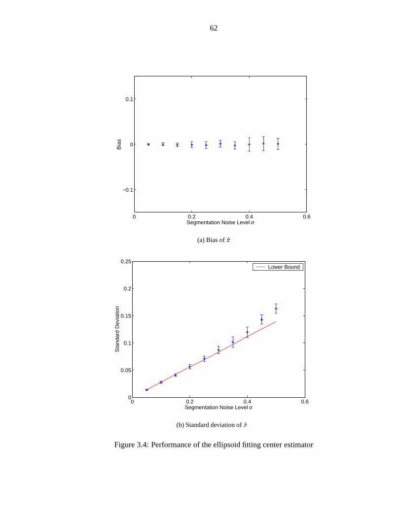
62

0 0.2 0.4 0.6

−0.1

0

0.1

Segmentation Noise Level σ

Bia

s

(a) Bias ofx

0 0.2 0.4 0.60

0.05

0.1

0.15

0.2

0.25

Segmentation Noise Level σ

Sta

ndar

d D

evia

tion

Lower Bound

(b) Standard deviation ofx

Figure 3.4: Performance of the ellipsoid fitting center estimator

CHAPTER IV

APPLICATIONS OF STATISTICAL POLAR SHAPEMODELING

The statistical polar shape models have been introduced in Chapter II. We will look

at two applications of statistical shape modeling in this chapter. The first application of

Wiener filtering intends to show how the orthogonal representation of a random field can

be applied to optimal shape filtering and estimation. The second application to 3D ob-

ject registration demonstrates that linear transform method is still a very effective tool in

pattern recognition. In particular, the independence of the random shape parameters can

efficiently reduce the computational complexity of optimization procedure.

4.1 Wiener Filtering on Unit Sphere

Shape extraction is a noisy process that introduces boundary approximation errors. If

we can model the extracted shape as an isotropic random field overS2, as discussed in

Section 2.3, Wiener filtering can yield an optimal shape estimator in terms of the least

mean square error.

4.1.1 Wiener filtering by spherical harmonics

It has been shown that spherical harmonics are eigenfunctions in the Karhunen-Lo´eve

expansion of an isotropic random field over the unit sphereS2. It is well known that

63

64

Wiener filtering can be implemented in the original or K-L expansion domains. Based on

the spectral theory of isotropic random field and the spherical geometry of polar objects,

one can also in principle use this theory to decompose the radial function and estimate

independent noisy shape parameters. The detailed procedure is described in the text fol-

lowing.

Let F (x) : S2 ! (0;+1) represent the radial function of a polar object acquired

through some segmentation process. It is assumed that�F = E[F ] and that the zero mean

random fieldF � �F can be decomposed as:

F (x)� �F (x) = S(x) +W (x) (4.1)

whereS is an isotropic zero mean Gaussian random field andW represents a white

Gaussian noise field. The correlation function ofS can be represented byRS(x; y) =

S(cos(](x; y))). Strictly speaking, for consistencyS andW must be such thatS+W �� �F w.p.1. We will sidestep this issue by assuming that the standard deviations ofS andW

are much smaller than�F . By spectral theory of isotropic random field, the K-L expansion

of S is a linear combination of spherical harmonics,

S(x) =1Xl=0

lXm=�l

aml Yml (x) (4.2)

whereaml is independent random variable (for alll; m) with zero mean and variance

E[aml am0

l0 ] = �lÆl;l0Æm;m0 : (4.3)

Here�l is determined by�l = 2�R 1

�1 S(x)Pl(x)dx. Let �2W be the variance of the white

Gaussian noise andFml =

RS2(F � �F )Y m

l (x)dS2 be the spherical harmonic coefficients

of F � �F . By Wiener filtering theory, the optimal estimator of the parameteraml is the

conditional meanE[aml jFml ] which can be written as:

aml =

RS2(F � �F )Y m

l (x)dS2 � �l�l + �2W

: (4.4)

65

The optimal estimation ofS is a linear combination of spherical harmonics weighted by

aml :

S(x) =1Xl=0

lXm=�l

aml Yml (x) (4.5)

For the theory of Wiener filtering, readers are referred to [94] for details.

4.1.2 Double Fourier Series Approximation

To reduce the computational complexity of spherical harmonics, double Fourier series

can be introduced in place of spherical harmonics in the estimation procedure.

The Legendre polynomialPl(cos �) can be written as

Pl(cos �) =lX

k=0

(�1)n��1

2

k

�� �12

l � k

�cos(l � 2k)�: (4.6)

And the associated Legendre functionPml (x) has the following relationship withPl(x)

Pml (x) = (�1)m(1� x2)m=2 d

m

dxmPl(x) (4.7)

Therefore the spherical harmonics functionY ml (�; �) = cml P

ml (cos �)eim� has an inherent

relationship with double Fourier series and can be rewritten as a linear combination of

double Fourier series. We relate double Fourier series to spherical harmonics by repre-

senting a finite number of discretized spherical harmonics and double Fourier series basis

elements in two matrices� and, respectively. LetK represent the constant matrix which

maps the DFS basis onto the SH basis�: � = K. The rank ofK only depends on the

highest order of SH used in the application. It can be shown thatK is a very sparse matrix

and therefore has a fast inverse algorithm [104]. Table 4.1.2 shows the total number of

nonzero elements inK for different highest order of spherical harmonics. Here the double

Fourier series are in the format as 2.21.

This motivates the following algorithm for Wiener filtering over the unit sphere. First,

compute the double Fourier series of the radial functionF . Second, the coefficients of

66

Table 4.1: The total number of nonzero entries in sparse mapping matrixK vs. the highestoder of spherical harmonics basis.

Highest order of basis 2 3 4 5 6Size ofK 9� 36 16� 64 25� 100 36� 144 49� 196

# of nonzero entry 10 22 41 70 110

double Fourier series are converted to the coefficients of spherical harmonics through the

transformationK. After the optimal estimation of spherical harmonics coefficients is ob-

tained through Wiener filtering, they can be mapped back to double Fourier series viaK.

4.1.3 Experiment Results

01

23

4

0

2

4

6

8−0.015

−0.01

−0.005

0

0.005

0.01

0.015

θφ

Bia

s

(a) Bias

01

23

4

0

2

4

6

80

0.05

0.1

0.15

0.2

θφ

Var

ianc

e

(b) Variance

Figure 4.1: Comparison of linear filtering and Wiener filtering results onS2. Red surfacesrepresent the results of linear filtering and blue surfaces represent the resultsof Wiener filtering.

Applying the spectral theory of isotropic random field, we simulated an isotropic ran-

dom field over the unit sphere through following steps: First, the covariance function of

the random field (cos ) is decomposed to obtain the value of�l. Second, the set of inde-

pendent random coefficientsfAml g is simulated by multiplying�l with i.i.d Gaussian ran-

dom variables. Finally, the isotropic random fieldX(�; �) is obtained by combining finite

number of spherical harmonic basis functions, i.e.,X(�; �) =PL

l=0

Plm=�l A

ml Y

ml (�; �):

67

White Gaussian noise is added toX.

To evaluate the performance of Wiener filtering, we compared it with the linear filtering

result. The linear filtering is implemented through a convolution with an average filter.

5000 samples of the random field were generated in the experiment. Figure 4.1(a) shows

the bias of Wiener filtering and linear filtering results of the same random field. The red

rough surface represents the bias of the linear filtering result, while the relatively flat blue

surface represents the bias of Wiener filtering result. It can be seen that the result of Wiener

filtering is biased since the blue surface is a little bit below the zero-plane. This is because

Wiener filtering tends to shrink the object to a sphere. Alternatives would require a “non-

isotropic” filter. In Figure 4.1(b), the variances of the two filtering results are plotted. It

can be seen that the Wiener filtering result (blue surface) has a much smaller variance than

the linear filtering result(red surface).

4.2 Estimation of 3D Rotation in Image Registration

4.2.1 Review

Finding the rotation of a 3D object is a common problem. A 3D rigid motion maps

a 3D image data set to another set. This registration procedure is to align 3D images in

a common coordinate system. By computing the centroid of each set, one can translate

them in space so that their centroids come to a common coordinate origin. A remaining

problem is to determine the 3D rotation between the sets of data. Most techniques for fit-

ting 3D rotation to 3D data estimate the 3D rotation in the spatial domain [62], and usually

are of very high computational complexity. Considering the registration of a single 3-D

object, Burel [19] proposed to use spherical harmonics as orthogonal basis to decompose

the 3D shapes and get the invariants for object recognition. We here develop a maximum

likelihood (ML) method to jointly estimate the spherical harmonics coefficients and the

68

Euler angles of 3D rotation based on Burel’s method. The novelty of our method lies on

its use of the assumption that the noise field is isotropic Gaussian and thus the decom-

posed noise coefficients are statistically independent. Since the 3D objects are registered

in the frequency domain via low order spherical harmonic coefficients, the registration

automatically filters out high frequency noise and has low computational complexity.

4.2.2 Representation ofSO(3) by Spherical Harmonics

The degree of freedom of any rotationg in SO(3) is three andg can be defined in

terms of Euler angles�; �; . In other words, a rotationg which carries the axisx; y; z

to new positionsx0; y0; z0, can be accomplished by three successive rotations around the

coordinate axes, namely a rotation around thez axis through an angle�, a rotation around

the new direction of they axis through an angle� and a rotation around the new direction

of z axis through an angle . Thus,g has the matrix product representation:

Rg = Rz(�) Ry(�) Rz( ): (4.8)

In terms of group theory, the spherical harmonics expand an irreducible representation

space of the rotationg [105]. This means the representation space of the rotationg 2

SO(3) can be decomposed into a direct sum of orthogonal subspaces which are globally

invariant by rotation, i.e.,

Ł = D(0) �D(1) �D(2) �D(3) � � � � �D(l) � � � � (4.9)

where Ł is the linear representation space of the groupg andD(l) denotes a(2l + 1)-

dimensional invariant subspace of Ł. The basis forD(l) is Y ml (�; �); m = �l : : : l.

Let the global shape function of a 3D object have a spherical harmonic representation:

R(�; �) =KXl=0

lXm=�l

cml Yml (�; �): (4.10)

69

Applying the 3D rotation operatorg to the objectR(�; �) gives a new radial function

~R(�; �) = g(R(�; �)), which can also be decomposed by spherical harmonics:

~R(�; �) =KXl=0

lXm=�l

~cml Yml (�; �): (4.11)

The spherical harmonic coefficients~cml in (4.11) andcml in (4.10) have the following rela-

tionship [105]:0BBBBBBBBBBBBBBBBBBBBBBBBBBBBBB@

~c00

~c�11

~c01

~c11

~c�22

~c�12

~c02

~c12

~c22

...

1CCCCCCCCCCCCCCCCCCCCCCCCCCCCCCA

=

0BBBBBBBBBBBBBBBBBBBBBBBBBBBBBB@

D(0) 0BBBBB@ D(1)

1CCCCCA 0BBBBBBBBBBBB@D(2)

1CCCCCCCCCCCCA. . .

1CCCCCCCCCCCCCCCCCCCCCCCCCCCCCCA

0BBBBBBBBBBBBBBBBBBBBBBBBBBBBBB@

c00

c�11

c01

c11

c�22

c�12

c02

c12

c22

...

1CCCCCCCCCCCCCCCCCCCCCCCCCCCCCCAwhich can also be written as

~cml =lX

m0=�lDlmm0(�; �; )cm

0

l (4.12)

where,

Dlmm0(�; �; ) = exp(�im�) � dlmm0(�) � exp(�im0 ) (4.13)

and

dlmm0(�) = (�1)l�m0p

(l +m)!(l �m)!(l +m0)!(l �m0)!

�Xk

(�1)k (cos �2)m+m0+2k(sin �

2)2l�m�m

0�2k

k!(l �m� k)!(l �m0 � k)!(m+m0 + k)!: (4.14)

70

In (4.14), the summation is carried out over all values ofk producing positive integers

under the factorial symbol.

Example: The matrixdlmm0(�) for 0 � l � 2. Let c = cos � ands = sin�. Then,

d0(�) = 1

d1(�) =

0BBBBB@1+c2

� sp2

1�c2

sp2

c � sp2

1�c2

sp2

1+c2

1CCCCCA

d2(�) =

0BBBBBBBBBBBB@

�1+c2

�2 � (1+c)2s

p64s2 � (1�c)

2s

�1�c2

�2(1+c)

2s (1+c)

2(2c� 1) �

q32sc (1�c)

2(2c+ 1) � (1�c)

2s

p64s2

q32sc 1

2(3c2 � 1) �

q32sc

p64s2

(1�c)2s (1�c)

2(2c+ 1)

q32sc (1+c)

2(2c� 1) � (1+c)

2s�

1�c2

�2 (1�c)2s

p64s2 (1+c)

2s

�1+c2

�2

1CCCCCCCCCCCCA:

4.2.3 Estimation of 3D Rotation

In section 4.2.2, it is shown that the relationship between two sets of spherical harmon-

ics coefficients describing the surface functions of a 3D object in different orientations can

be uniquely determined by a rotationg 2 SO(3). In fact, the rotationg 2 SO(3) maps

the vector space of the spherical harmonic coefficients to the same space, and the mapping

is one-to-one and onto. However, different sets of Euler angles may lead to the same ro-

tationg, which means the solution to the inverse problem of Euler angle estimation is not

unique. We can either arbitrarily pick one solution or obtain a unique solution by adding

some constraints. The rest of this section discusses the rotation estimation using spher-

ical harmonics for objects whose noise fields are isotropic Gaussian random fields (See

Appendix B).

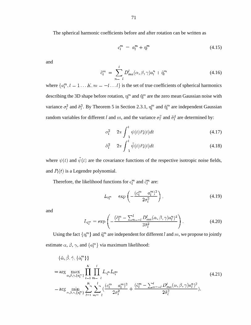
71

The spherical harmonic coefficients before and after rotation can be written as

cml = aml + �ml (4.15)

and

~cml =lX

n=�lDlmn(�; �; )a

nl + ~�ml (4.16)

wherefaml ; l = 1 : : :K;m = �l : : : lg is the set of true coefficients of spherical harmonics

describing the 3D shape before rotation,�ml and~�ml are the zero mean Gaussian noise with

variance�2l and~�2l . By Theorem 5 in Section 2.3.1,�ml and~�ml are independent Gaussian

random variables for differentl andm, and the variance�2l and~�2l are determined by:

�2l = 2�

Z 1

�1

(t)Pl(t)dt (4.17)

~�2l = 2�

Z 1

�1

~ (t)Pl(t)dt (4.18)

where (t) and ~ (t) are the covariance functions of the respective isotropic noise fields,

andPl(t) is a Legendre polynomial.

Therefore, the likelihood functions forcml and~cml are:

Lcml= exp

��(cml � aml )

2

2�2l

�; (4.19)

and

L~cml= exp

�(~cml �

Pln=�lD

lmn(�; �; )a

nl )

2

2~�2l

!: (4.20)

Using the factf�ml g and~�ml are independent for differentl andm, we propose to jointly

estimate�, �, , andfaml g via maximum likelihood:

f�; �; ; faml gg

=arg max�;�; ;fam

lg

KYl=1

lYm=�l

LcmlL~cm

l

=arg min�;�; ;faml g

KXl=1

lXm=�l

((cml � aml )

2

2�2l+

(~cml �Pl

n=�lDlmn(�; �; )a

nl )

2

2~�2l):

(4.21)

72

Note that the maximum likelihood estimate is equivalent to a weighted least squares

fitting problem, which is a nonlinear optimization here. As is the case with many such

implicitly defined estimators, the minimum can not be found analytically and iterative

minimization of the objective should be employed.

4.2.4 Cramer-Rao Bound for Joint Estimation

To evaluate the performance of joint estimation of spherical harmonics coefficients and

rotation angle, we derive the Cram´er-Rao lower bound for the variance of the estimator.

Let L = � lnQl

m=�l p(cml jaml )p(~cml jffaml g; �; �; g). Take derivative ofL overakl ,

we get

@L

@akl= �(ckl � akl )

�2l�Pl

m=�l(~cml �

Pln=�lD

lmna

nl ) �Dl

mk

~�2l: (4.22)

And the second order derivative ofL overakl is

@2L

@(akl )2=

1

�2l+

Plm=�l(D

lmk)

2

~�2l: (4.23)

The Fisher information of the coefficients is:

E[@2L

@akl2 ] =

1

�2l+

Plm=�l E[(Dl

mk)2]

~�2l: (4.24)

The second term in the above equation demonstrates the profit of joint estimation. The

Cramer-Rao bound which is just the inverse of the Fisher information matrix is thus ob-

tained. Similarly, we can derive the lower bound for the rotation angle estimator. We will

compare the variance of the estimators with these lower bounds in the next section.

4.2.5 Experimental Results

The proposed estimation method has been implemented to jointly estimate the 3D

rotation and spherical harmonic coefficients of the noise contaminated objects. The inputs

to the joint estimator are two sets of noisy spherical harmonic coefficients which can be

73

modeled by (4.15) and (4.16). For each given noise level,500 independent realizations of

the Gaussian noise field were generated for each set of the spherical harmonic coefficients.

The mean values of the second set of spherical harmonic coefficients are determined by

the product of the mean values of the spherical harmonic coefficients in the first set and

the 3-D rotation matrix. For computation convenience, we set�2l = ~�2l . Only the first

order of spherical harmonics coefficients(c�11 ; c01; c

11) and(~c�1

1 ; ~c01; ~c11) have been used in

the optimization procedure. Higher order coefficients can, of course, be used for the fine

tuning, but it will correspondingly increase the computation burden of optimization. The

Levenberg-Marquardt algorithm with a mixed quadratic and cubic line search procedure

was used via MATLAB functionlsqnonlin( ) to find the estimates of Euler angles and

shape parameters.

0 0.1 0.2 0.3−0.5

0

0.5

σ

Bia

s

(a) Coefficienta01

0 0.1 0.2 0.3−0.5

0

0.5

σ

Bia

s

(b) Rotation Angle�

Figure 4.2: Biases of a shape parameter estimator and a rotation angle estimator.

The measured biases of the estimatorsa01 and� are plotted versus the standard devi-

ation of the Gaussian noise in Figure 4.2. From the observed data, we can say that the

estimator is basically unbiased. The fact that measured bias deviates from zero, is due to

insufficient number of Gaussian noise processes generated in the simulation.

In Figure 4.3, the standard deviations ofa01 and� are compared to the corresponding

74

0 0.1 0.2 0.30

0.1

0.2

0.3

0.4

0.5

σ

Sta

ndar

d D

evia

tion

Lower Bound

(a) Coefficienta01

0 0.1 0.2 0.30

0.1

0.2

0.3

0.4

0.5

σ

Sta

ndar

d D

evia

tion

Lower Bound

(b) Rotation Angle�

Figure 4.3: Comparison between the estimators’ standard deviations and the Cram´er-Raobounds.

Cramer-Rao lower bounds. It can be seen that the standard deviation of the estimators is

less than the standard deviation of the noise process. Therefore, the joint estimation has

improved the performance of the shape parameter estimator. Since the boundary informa-

tion in the two sets of images is correlated, this is an expected result. The performances

of the two estimators are close to the lower bounds, which shows they are near efficient

estimators.

CHAPTER V

SPECTRAL METHOD TO SOLVE ELLIPTICEQUATIONS IN SURFACE RECONSTRUCTION AND

3D ACTIVE CONTOURS

5.1 Introduction

Automatic recovery of 3D object shapes from various image modalities is an important

research area in computer vision and image processing. This task can be accomplished

in two steps. First, the object is segmented from the 3D image. Segmentation data is

usually stored in the form of coordinates of sampled surface points. Second, a surface

reconstruction algorithm is applied to filter the noise in segmentation data and achieve

a shape representation of the object. In the last two decades, active contour methods

(deformable models) have been developed to solve the segmentation and reconstruction

problems simultaneously. Active contours can evolve towards the object boundary under

some regularizations. The evolution is controlled by a partial differential equation, where

segmentation and reconstruction functions are represented by two different terms in the

equation. The existing active contour approaches can be classified into two categories:

parametric active contours and geometric active contours.

The class of parametric active contour originates from the “snake” introduced by Kass

[63] which uses energy-minimizing curve to locate boundaries in 2D imagery. The dif-

75

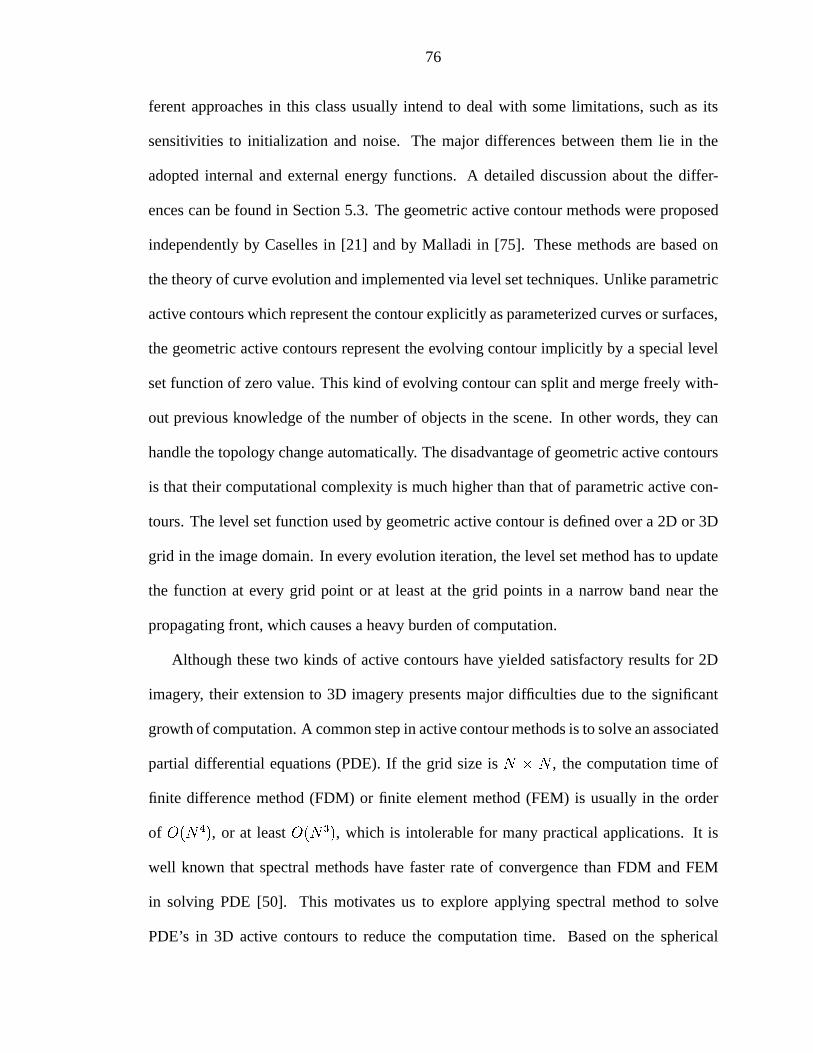
76

ferent approaches in this class usually intend to deal with some limitations, such as its

sensitivities to initialization and noise. The major differences between them lie in the

adopted internal and external energy functions. A detailed discussion about the differ-

ences can be found in Section 5.3. The geometric active contour methods were proposed

independently by Caselles in [21] and by Malladi in [75]. These methods are based on

the theory of curve evolution and implemented via level set techniques. Unlike parametric

active contours which represent the contour explicitly as parameterized curves or surfaces,

the geometric active contours represent the evolving contour implicitly by a special level

set function of zero value. This kind of evolving contour can split and merge freely with-

out previous knowledge of the number of objects in the scene. In other words, they can

handle the topology change automatically. The disadvantage of geometric active contours

is that their computational complexity is much higher than that of parametric active con-

tours. The level set function used by geometric active contour is defined over a 2D or 3D

grid in the image domain. In every evolution iteration, the level set method has to update

the function at every grid point or at least at the grid points in a narrow band near the

propagating front, which causes a heavy burden of computation.

Although these two kinds of active contours have yielded satisfactory results for 2D

imagery, their extension to 3D imagery presents major difficulties due to the significant

growth of computation. A common step in active contour methods is to solve an associated

partial differential equations (PDE). If the grid size isN � N , the computation time of

finite difference method (FDM) or finite element method (FEM) is usually in the order

of O(N4), or at leastO(N3), which is intolerable for many practical applications. It is

well known that spectral methods have faster rate of convergence than FDM and FEM

in solving PDE [50]. This motivates us to explore applying spectral method to solve

PDE’s in 3D active contours to reduce the computation time. Based on the spherical

77

geometry of star-shaped object, we propose a new parametric active contour method which

uses double Fourier series as the orthogonal basis to solve the PDE defined on the unit

sphere. The method is applied to segment both synthesized 3D images and X-ray CT

images. It is shown that the new method preserves the merits of other parametric active

contour methods while significantly reducing the computation time. Due to the generality

of our mathematical formulation, the method can be easily applied to solve the surface

reconstruction problem.

Throughout this chapter, the following notations are used:

I(x; y; z), 3D grey-level image;

x(u; v), surface function in Cartesian coordinates;

f(�; �), admissible surface function in spherical coordinates;

g(�; �), noisy radial function obtained from segmentation;

g := xg; yg; zg, a set of coordinates of detected edge points;

gf(�; �), segmentation data detected by propagating contourf ;

d(), Euclidean distance function;

� and�, parameters controlling tradeoff.

5.2 Surface Reconstruction of Star-Shaped Object

Let g(�; �) be a noisy radial function obtained from the segmentation of a star-shaped

object. The surface reconstruction problem is to use some form of regularization to ap-

proximate the noisy functiong(�; �) by a smooth reconstruction functionf(�; �). Usually

[27], the solutionf is a critical point which minimizes the energy functional defined in the

form:

E(f; g) = �

ZS2Y (f; g)d +

ZS2Z(f)dS2 (5.1)

78

whereY measures the distance between the functionf and the coarse segmentation data

g, Z is a measure of reconstruction smoothness, and� controls the tradeoff between the

faithfulness to the segmentation data and the smoothness. The two terms inE represent

the faithfulness to the segmentation data and the regularization penalty, respectively. If

we define the data fidelity metricY (f; g) = (f(�; �) � g(�; �))2, the approach becomes

least squares fitting which is a classic reconstruction method. The regularization term

frequently contains the derivative of the functionf to enforce smoothness. For instance,Z

can be defined to beZ(f) = krfk2, wherer is the gradient operator. With these choices,

the energy functional is completely defined,

E(f; g) =

ZS2�(f(�; �)� g(�; �))2dS2 +

ZS2krf(�; �)k2dS2 : (5.2)

The reconstruction objective is to minimizeE(f; g) overf . Using the calculus of varia-

tions [32], the critical point of the above energy functional can be found by solving the

associated Euler-Lagrange equation (See Appendix C):

r2f � �(f � g) = 0: (5.3)

This is an elliptic equation of Helmholtz type on the sphere [6]. Although finite differ-

ence methods (FDM) and finite element methods (FEM) can be employed to solve this

equation, their computational complexities are higher than the spectral method that will

be introduced in Section 5.4. For this surface reconstruction problem, elliptic PDE can be

solved by spectral method in only one iteration. In the next section, we will show that a

PDE similar to (5.3) has to be solved to control the evolution of parametric active contour.

It can be solved by the fast spectral method sequentially.

79

5.3 Parametric Active Contours

As mentioned in the introduction of this chapter, parametric active contour methods

can solve the segmentation problem and the reconstruction problem simultaneously. A

surfacex in IR3 is a mapping:x(u; v) = (x1(u; v); x2(u; v); x3(u; v)), i.e. x : ! IR3,

where is a subset ofIR2 [51]. If x represents a propagating surface in a parametric active

contour approach, an energy functionalE associated withx can be defined:

E(x) =

Z

�[�krxk2 + �kr2xk2] + Pext(x)

�d (5.4)

where� and� are the parameters controlling the smoothness ofx andPext represents a

potential function. It is clear that two kinds of energy constitute the energy functional. The

termR�krxk2 + �kr2xk2d, which is computed from the contourx itself, is called

internal energy. The termRPext(x)d, which is computed from the image and current

location ofx, is called external energy. The force generated by the internal energy dis-

encourages the stretching and bending of the contour, in other words, has regularization

effect on the contour, while the force generated by the external energy attracts the contour

towards the object boundary. Therefore, the external energy represents the segmentation

function of the active contour, and the internal energy represents the reconstruction func-

tion of the active contour. The contourx deforms under these two kinds of forces to find a

minimizer of the energy functionalE.

5.3.1 External Force Field

The external force field plays an important role in active contour methods. Typically,

active contours are drawn towards the desired boundary by the external force which could

include one or more of the following components: a traditional potential force, obtained by

computing the negative gradient of an attraction potential defined over the image domain

80

I

ogf

d(g,f)

g

x

f

d(g,x) or

Figure 5.1: An grey level imageI, the set of edge pointsg detected inI, a propagatingcontourf , andd(g;x) ord(g; f), the distance between the propagating contourand its nearest edge point.

[27, 63]; a pressure force, used by Cohen in his balloon model [27], which could be either

expanding or contracting depends on whether the contour is initialized from inside or

outside; or a gradient vector flow, used by Xu [108] and obtained by diffusion of edge-

map’s gradient. The role of the external force is such that it must contain the information

of boundary and must have sufficient capture range.

Let I(x; y; z) represent the image to be segmented,g := xg; yg; zg be the set of all

edge points detected inI, andd(g; (x; y; z)) be the distance from a point(x; y; z) in the

evolving surfacex to its nearest edge point, i.e.dg(x; y; z)�= min(xg ;yg;zg)2g k(x; y; z) �

(xg; yg; zg)k. Figure 5.1 illustrates the relation between these denotations. Potential func-

tions designed to deform the active contour usually have a global minimum at the object

boundary. Two common types of potential functions are:

P(1)(x) = h1(rI(x)) (5.5)

P(2)(x) = h2(d(g;x)) (5.6)

81

whereh1 andh2 are functions makingP(1) andP(2) convex in at the location of object

boundary. For instance,P (x; y; z) = �jrI(x; y; z)j2, P (x; y; z) = �jrG�(x; y; z) �

I(x; y; z)j2 andP (x; y; z) = 11+jrIjp belong to the type ofP(1). In fact, jrIj serves as

an edge detector which locates sharp intensity changes in imageI. Although the use of

Gaussian filterG� can blur boundaries, it is often necessary to use it to increase the capture

range of the external force or to deal with the disconnected edges. Figure 5.2 illustrates the

attraction force generated by a potential function in1D case. Potential functions of type

x

I

(a) The imageI

x

G*I

(b) Smoothed imageI �G�

x

P

(c) P = �krI � Gk2 andexternal forceF = �rP

Figure 5.2: Interpretation of attraction potentialP

P(1) have the disadvantage that the resulting external force has very small capture range

becauseP(1) t 0 in intensity homogeneous areas. Potential functions of typeP(2) solve

this problem by incorporating the use of edge points extracted by local edge detectors.

The common choices ofP(2) areP (x; y; z) = d2(g; (x; y; z)), P (x; y; z) = �1d(g;(x;y;z))

and

P (x; y; z) = �e�d2(g;(x;y;z)). The boundary location has been broadcasted to many of

their neighbors through the value ofd. In our experiment, we chosed2(g;x), aP(2) type

potential function, to generate the external force for the active contour. This external force

will evolve the active contour towards the boundary along a path of minimal distance.

82

5.3.2 Regularization of Active Contour

In (5.4),�krxk2 and�kr2xk2 control the active contour’s elasticity and rigidity sep-

arately. The regularization effect coming from�krxk2 can be interpreted as a curvature

based flow which has very satisfactory geometric smoothing properties [66, 84]. Figure

5.3 shows the motion of a curve under curvature. The curve moves perpendicular to the

Figure 5.3: Motion of curve under curvature. The blue arrows represent negative curva-tures, while the red arrows represent the positive curvatures.

curve with speed proportional to the curvature. The curve motion is outward (inward)

where the curvature is negative (positive). A theorem in differential geometry states that

any simple closed curve moving under its curvature collapses to a circle and then disap-

pears. Therefore, a bigger� implies a bigger stretching force, so that the active contour

resists more the stretching, tends to shrink and have an intrinsic bias toward solutions that

reduce the active contour curve length or surface area. On the other hand, a bigger� im-

plies a larger resistance to tensile stress and bending. Therefore,� is often set to zero to

allow the active contour to become second-order discontinuous. The equation (5.4) is then

reduced to

E(x) =

Z

�krxk2 + d2(g;x)d (5.7)

83

For polar shape contours, it will be convenient to convert the surfacex expressed inIR3,

into a radial functionf(�; �) which expresses the surface in the object-centered spherical

coordinate system. This conversion not only simplifies the contour expression, but also

speeds up the contour evolution by allowing spectral method to solve PDE overS2. The

distance function then takes the form of

d(g;x) = d(g; f) � kf(�; �)� gf(�; �)k (5.8)

wheregf is defined as

gf(�; �)�=

argmin(xg;yg;zg)2g

k(xg; yg; zg)� (f sin � cos�; f sin � sin�; f cos �)k � (xo; yo; zo)

(5.9)

and(xo; yo; zo) represents the coordinates of object center (see Figure 5.1). The equation

(5.7) can then be rewritten as:

E(f) =

ZS2�krfk2 + (f � gf)

2dS2: (5.10)

Although equation (5.10) is analogous to equation (5.2), its associated Euler-Lagrange

equation is a little different as compared to equation (5.3). Sincegf is a non-linear function

of f , the calculus of variations leads to a more complicated Euler-Lagrange equation:

�r2f � (f � gf)(1� @gf@f

) = 0 (5.11)

There is no analytical expression for@gf@f

, so we approximated this by difference method

in our experiment. To apply the fast spectral method to solve this elliptic PDE, it has

to be manipulated so that it becomes a Helmholtz type PDE. We will describe such a

manipulation in Section 5.3.4 after we introduce another penalization term into this PDE

to deal with a “boundary leakage” problem.

84

5.3.3 Volumetric Penalization

Traditional parametric and geometric active contours solely rely on the local edge

detector to stop the curve propagation. These methods do not use any region-based or

volume-based information in the image. Such active contours can only segment and re-

construct objects which boundaries are well defined by gradientjrIj of the image. For

objects with very smooth or even broken boundaries, traditional active contour may pass

through the boundary. In [23], Chan proposed to use Mumford-Shah energy functional

[81] to deal with this “boundary leakage” problem. Similar approaches to include region-

based information can also be found in [61] and [97]. We use the same method as in [23]

to incorporate the volume information into the energy functional of 3D active contour. The

volume information is introduced as an additional penalty function

Evol(f) =

�Zinside(f)

(I � uin)2dV +

Zoutside(f)

(I � uout)2dV

�(5.12)

=

ZS2

Z f(�;�)

r=0

(I � uin)2r2dr +

Z B(I)

f(�;�)

(I � uout)2r2dr

!dS2

!

whereI = I(r; �; �) is the gray level intensity of the 3D image,B(I) represents the

boundary of the imageI, anduin anduout are the mean intensities in the interior of the

evolving surfacef and respectively outsidef

uin =

Rinside(f) IdV

vol(inside(f)); uout =

Routside(f) IdV

vol(outside(f)): (5.13)

Here the denominators are the volume inside and outside the evolving surface. The energy

function (5.13) can be adjoined to the Lagrangian (5.10) by aggregating the integrals over

S2:

E(f) =

ZS2

��krfk2 + (f � gf)

2 +

hZ f

0

(I � uin)2r2dr +

Z B(I)

f

(I � uout)2r2dr

i�dS2 (5.14)

85

Now calculus of variations can be applied to obtain the necessary condition for minimiza-

tion of this volumetrically penalized Lagrangian

�r2f � (f � gf)(1� @gf@f

)� z(f; I) = 0 (5.15)

where

z(f; I) = f 2 � [(I(f)� uin)2 � (I(f)� uout)

2] + 2(ÆuinÆf

)

Z f

0

r2(I � uin)dr

+2(ÆuoutÆf

)

Z B(I)

f

r2(I � uout)dr (5.16)

and

ÆuinÆf

=

RS2f 2I(f)dS2 � uin surf(f)

vol(inside(f))(5.17)

ÆuoutÆf

= �RS2f 2I(f)dS2 � uout surf(f)

vol(outside(f))(5.18)

where surf(f) =RS2f 2dS2 is the surface area of the evolving contour.

5.3.4 Evolution Algorithm

Comparing equation (5.15) with (5.3), it is clear the Euler-Lagrange equation (5.15)

is no longer a Helmholtz PDE. First, the functional dependence ofgf on f makes the

equation non-linear inf . Second, the additive volumetric penalization termz is not linear

in f and is not “instantaneous” in(�; �). The same issue was encountered in [61] and

the authors got around it by linearization ofz with fn+1 = fn and update propagation

over (�; �). “Update propagation” means that for iterationn + 1, we updatefn in terms

of past iteratefn(�0; �0) if fn+1 for (�0; �0) has not yet been computed, and partial update

fn+1(�0; �0) if fn+1 for (�0; �0) has been computed. This idea can be similarly applied to

linearize equation (5.15) so that it has a Helmholtz format which can be solved by the fast

spectral method. Combining all the non-linear terms into a single bundle and move it to

86

the right side of the equation, (5.15) is rewritten as:

�r2f � f = z(f; I)� (f � gf)@gf@f

� gf : (5.19)

Due to the non-linearity of equation (5.19), it has to solved iteratively. In then+1 iteration,

the right hand side of (5.19) will be updated with the value offn so that the equation

becomes a new Helmholtz PDE, i.e.

�r2fn+1 � fn+1 = z(fn; I)� (fn � gfn)@gfn@fn

� gfn (5.20)

The details of the evolution algorithm is as following:

1. Initialize the evolution withf0 = c, c is determined by the object size;

2. Computegfn(�; �) and update the RHS of (5.20) withfn andgfn;

3. Solve PDE�r2fn+1�fn+1 = z(fn; I)�(fn�gfn)@gfn@fn�gfn with spectral method

to get the new contourfn+1;

4. Compute the error,en+1 =

qPM�1

i=0

PN�1

j=0 (fn(�i;�j)�fn+1(�i;�j)2MN

5. if en > threshold, go back to 2,

else end.

In the above algorithm,� and are chosen in advance to control the tradeoff.

5.4 Spectral Methods for Solving PDE

As we have discussed in the last section, the implementation of active contours in-

volves solving partial differential equations. Finite difference [108] and finite element

[27] methods have been used to solve the associated Euler-Lagrange equations. However,

all of these methods have difficulties in 3D images due to the large grid size used in 3D

87

images. Spectral and pseudo-spectral methods have emerged as a viable alternative to fi-

nite difference and finite element methods for the numerical solutions of partial differential

equations. They are now widely used in the numerical simulation of turbulence and phase

transition, numerical weather prediction and the study of ocean dynamics where high ac-

curacy is desired for complicated solutions [8, 50, 101, 14, 111]. Since our problem is

in spherical geometry, basis functions such as spherical harmonics, double Fourier series

and Chebyshev polynomials, all have attractive features. A good comparison of these

functions is given by Boyd in [13]. The spherical harmonics are best with regard to the

pole problems (recall discussion in Chapter II) because of the property of the associated

Legendre functions, but the Legendre functions also make spherical harmonics the most

complicated to program and use among the three basis sets. On the other hand, double

Fourier series can give comparable accuracy and are significantly easier to program. Most

of all, the existing FFT makes double Fourier series the most efficient transform method.

Yee first applied truncated double Fourier series to solve Poisson-type equations on a

sphere [112]. Recently, Cheong proposed a new method which is similar to Yee’s method,

but removes the constraint that is imposed on the spectral coefficients and lead to increased

accuracy and stability in a time-stepping procedure [25]. We adopt this new method to

solve the associated Euler-Lagrange equation in the active contour evolution.

5.4.1 The Spectral Method

We describe the spectral method proposed by Cheong in this section. The elliptic

equation (5.3)r2f � �(f � g) = 0 is a Helmholtz equation. The Laplacian operatorr2

on the unit sphere is of form:

r2 =1

sin �

@

@�(sin �

@

@�) +

1

sin2 �

@2

@2�: (5.21)

88

We assume the value of functionf andg are given on the grid(�j; �k), �j = �(j +0:5)=J

and�k = 2�k=K, whereJ andK are the number of data points along the latitude and

longitude, separately. We can expand the functiong, and similarly forf , with a Fourier

series in longitude with a truncationM , e.g.,

g(�; �) =MX

m=�Mgm(�)e

im�k (5.22)

wheregm(�) is the complex Fourier coefficient given bygm(�) = 1K

PK�1k=0 g(�; �k)e

�im�k ,

�k = 2�k=K andK = 2M . The equation (5.3) can then be written as an ordinary differ-

ential equation:

1

sin �

d

d�

�sin �

d

d�fm(�)

�� m2

sin2 �fm(�) = �[fm(�)� gm(�)] (5.23)

The latitude functionfm(�) andgm(�) can be further approximated by the truncated sine

or cosine functions,

gm(�j) =PJ�1

n=0 gn;0 cosn�j; m = 0

gm(�j) =PJ

n=1 gn;m sinn�j; oddm (5.24)

gm(�j) =PJ

n=1 gn;m sin �j sinn�j; evenm 6= 0

The procedure of calculating spectral coefficientsgn;m was shown in Chapter II. After the

substitution of (5.25) into (5.23), we get an algebraic system of equations in Fourier space:

(n� 1)(n� 2) + �

4fn�2;m � n2 + 2m2 + �

2fn;m +

(n+ 1)(n+ 2) + �

4fn+2;m

= �[1

4gn�2;m � 1

2gn;m +

1

4gn+2;m]; m = 0, or odd (5.25)

and

n(n� 1) + �

4fn�2;m � n2 + 2m2 + �

2fn;m +

n(n + 1) + �

4fn+2;m

= �[1

4gn�2;m � 1

2gn;m +

1

4gn+2;m]; m even6= 0 (5.26)

89

wheren = 1; 3; � � � ; J � 1 for oddn, n = 2; 4; � � � ; J for evenn if m 6= 0 andn =

0; 2; � � � ; J � 2 for evenn, n = 1; 3; � � � ; J � 1 for odd n if m = 0. This says the

components of even and oddn are uncoupled for a givenm. The equations (5.25) and

(5.26) can be rewritten in matrix format,

Bf = Ag (5.27)

whereB andA are matrices of sizeJ=2� J=2 with tridiagonal components only,f andg

are column vectors whose components are the expansion coefficients offm(�) andgm(�).

For example, the subsystem for oddn looks like this:0BBBBBBBBBBBB@

b1;m c1

a3 b3;m c3

. . . .. . . . .

aJ�3 bJ�3;m cJ�3

aJ�1 bJ�1;m

1CCCCCCCCCCCCA

0BBBBBBBBBBBB@

f1;m

f3;m

...

fJ�3;m

fJ�1;m

1CCCCCCCCCCCCA=

0BBBBBBBBBBBB@

2 �1�1 2 �1

. . . . . . . . .

�1 2 �1�1 2

1CCCCCCCCCCCCA

0BBBBBBBBBBBB@

g1;m

g3;m

...

gJ�3;m

gJ�1;m

1CCCCCCCCCCCCAThe procedure to solve the equation (5.3) is as follows: First, we getgn;m, the spectral

components ofg(�; �) by double Fourier series expansion. Then the right hand side of

(5.27) is calculated to obtain the column vectorg1 = Ag. Finally, the tridiagonal matrix

equationBf = g1 is solved andf(�; �) is obtained by inverse transform offn;m. Notice

that the Poisson equationr2f = g is just a special case of Helmholtz equation, a slight

modification in the above algorithm will give the solution to Poisson equation. Other

90

simple elliptic equations, such as biharmonic equations can also be solved by this spectral

method.

5.4.2 Complexity Analysis

Let us consider an elliptic equation with a grid size ofN �N on unit sphere. If FEM

were used, there would be a total ofN2 variables with matrix sizeN2�N2. A crude Gauss

elimination method will requireO(N6) operations and the Gauss-Siedel relaxation will

requireO(N4) operations to converge. If the algorithms can use the fact that the matrix

is sparse, it may reduce the number of operations toO(N3). However the computational

complexity of the spectral method described above is onlyO(N2 logN) (see [25]). The

complexity of the spectral method on the unit sphere is in the same order as that of FEM

method applied on a grid over a rectangle.

5.5 Experimental Results

We now present the results of applying the spectral method to solve the elliptic equa-

tions involved in the problems of surface reconstruction and 3D active contours.

5.5.1 Surface Reconstruction

For the surface reconstruction problem, we apply the algorithm to some synthesized

segmentation data to show how to choose the regularization parameter� for different noise

levels and for different shapes. The object center is assumed to be known or to have been

estimated in advance.

In the first experiment, we investigate the optimum value of� for different shapes. The

reconstructions of a sphere and an ellipsoid are compared to illustrate the role of�. The

Gaussian segmentation noise has been introduced and the standard deviation of the noise

in each sample direction is the same. In Figure 5.4, the reconstruction error is plotted

91

versus the value of� for two shapes. The straight line represents the standard deviation of

the segmentation noise. The figure shows that for a simple shape which only contains low

spatial frequency, such as the sphere, the value of� should be as small as possible in order

to filter out segmentation noise, while for a shape containing higher spatial frequencies,

such as the ellipsoid,� should be optimized to control the tradeoff between denoising and

matching high spatial frequencies. The optimum value of� is between101 and102 for the

ellipsoid shape. If� is too small, we will lose the high frequencies contained in ellipsoid

shape. If� is too high, the segmentation noise can not be get rid of efficiently. This is due

to the fact that unweighted Laplace operator is adopted for roughness penalty. Therefore

it acts as the prior shape is a sphere. Possible improvement is to induce other priors via

weighted Laplacian.

100

101

102

103

104

105

106

10−2

10−1

µ

Sta

ndar

d D

evia

tion

of R

econ

stru

ctio

n E

rror

Noise levelSphereEllipsoid

Figure 5.4: Standard deviation of reconstruction error vs.� for different shapes

The optimum value of� not only changes with different shapes, but also with different

noise levels. In the second experiment, the choice of� for different segmentation noise

92

levels is investigated. Different levels of Gaussian noise are added to the ellipsoidal shape.

Figure 5.5 shows that� should be smaller for lowSNR segmentation data than for high

SNR segmentation data, which is as expected. The knowledge of� obtained in the recon-

struction problem can guide us to choose the value of� in active contour method which

has an inverse role as�.

100

101

102

103

104

105

106

10−2

10−1

100

µ

Sta

ndar

d D

evia

tion

of R

econ

stru

ctio

n E

rror

σ=0.05σ=0.20σ=0.60

Figure 5.5: Standard deviation of reconstruction error vs.� for different segmentationnoise levels

Three reconstructions of the same segmented ellipsoid are presented in Figure 5.6. The

smoothness of the reconstructed surfaces is determined by the value of�.

Surface reconstruction can be accomplished in one iteration by the spectral method,

while a single-grid relaxation algorithm may need more than100 iterations to reach the

converged result.

93

(a) segmentation data (b)� = 104

(c) � = 103 (d) � = 102

Figure 5.6: Reconstruction of an ellipsoid.

5.5.2 3D Parametric Active Contours

5.5.2.1 Liver Shape Extraction

In this experiment, we want to extract the shape of liver from X-ray CT images. Double

Fourier series were used to expand the radial function of the 3D contour. First, a set of

edge maps was derived from the256 � 256 CT slices by MATLAB functionedge( ). It

is the input to our 3D active contour method. The CT slices and the corresponding edge

maps are shown in Figure 5.7.

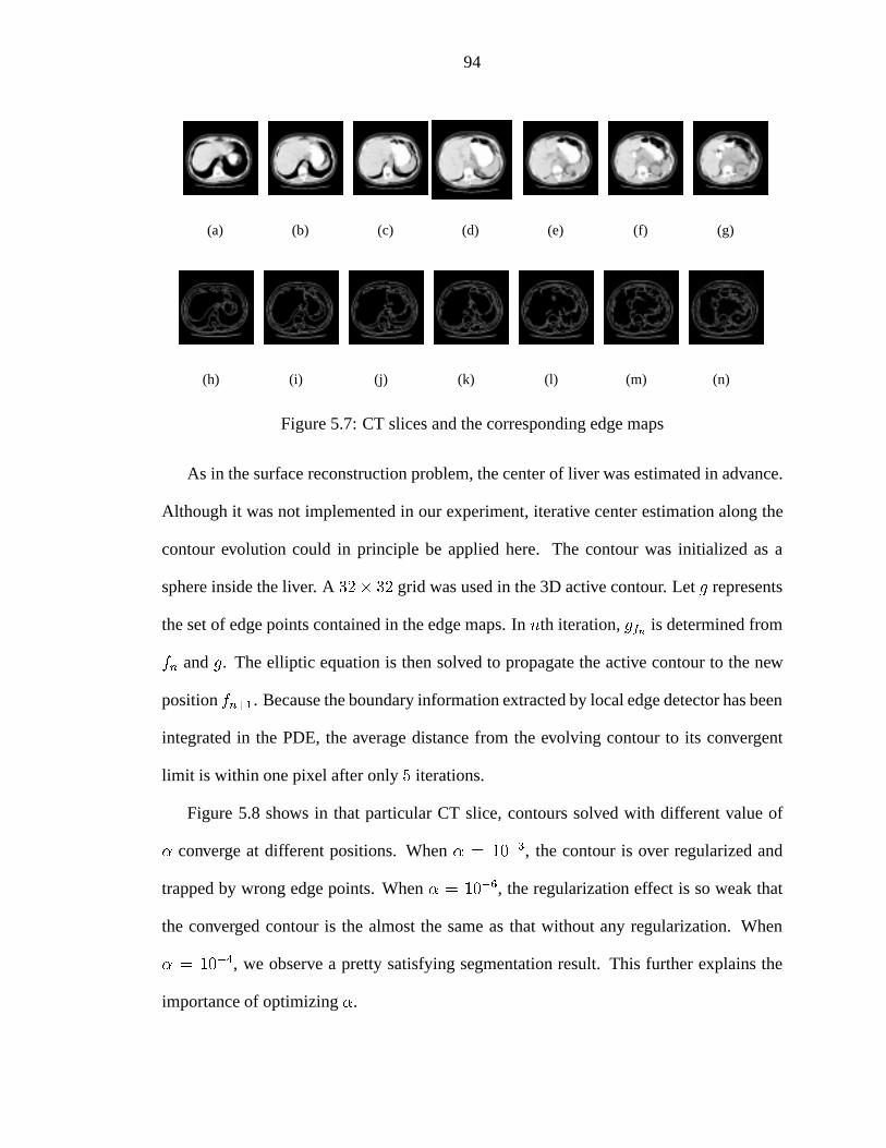
94

(a) (b) (c) (d) (e) (f) (g)

(h) (i) (j) (k) (l) (m) (n)

Figure 5.7: CT slices and the corresponding edge maps

As in the surface reconstruction problem, the center of liver was estimated in advance.

Although it was not implemented in our experiment, iterative center estimation along the

contour evolution could in principle be applied here. The contour was initialized as a

sphere inside the liver. A32� 32 grid was used in the 3D active contour. Letg represents

the set of edge points contained in the edge maps. Innth iteration,gfn is determined from

fn andg. The elliptic equation is then solved to propagate the active contour to the new

positionfn+1. Because the boundary information extracted by local edge detector has been

integrated in the PDE, the average distance from the evolving contour to its convergent

limit is within one pixel after only5 iterations.

Figure 5.8 shows in that particular CT slice, contours solved with different value of

� converge at different positions. When� = 10�3, the contour is over regularized and

trapped by wrong edge points. When� = 10�6, the regularization effect is so weak that

the converged contour is the almost the same as that without any regularization. When

� = 10�4, we observe a pretty satisfying segmentation result. This further explains the

importance of optimizing�.

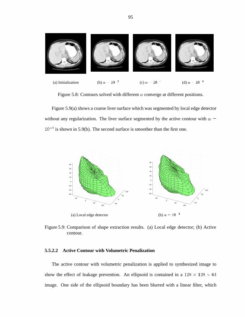
95

(a) Initialization (b)� = 10�3 (c)� = 10�4 (d)� = 10�6

Figure 5.8: Contours solved with different� converge at different positions.

Figure 5.9(a) shows a coarse liver surface which was segmented by local edge detector

without any regularization. The liver surface segmented by the active contour with� =

10�4 is shown in 5.9(b). The second surface is smoother than the first one.

−50

0

50

100−50

0

50

100

−60

−40

−20

0

20

40

60

80

(a) Local edge detector

−50

0

50

100

−50

0

50

100

−60

−40

−20

0

20

40

60

80

(b)� = 10�4

Figure 5.9: Comparison of shape extraction results. (a) Local edge detector; (b) Activecontour.

5.5.2.2 Active Contour with Volumetric Penalization

The active contour with volumetric penalization is applied to synthesized image to

show the effect of leakage prevention. An ellipsoid is contained in a128 � 128 � 64

image. One side of the ellipsoid boundary has been blurred with a linear filter, which

96

is shown in Figure 5.10(a). This blurred image and its edgemap are the inputs to the

new algorithm. Figure 5.10(b) shows that the traditional algorithm can not prevent the

contour from leaking at the blurred boundary. Figure 5.10(c) illustrates that the contour

with volumetric penalization can stop at the right place. The small fluctuation of the

converged active contour boundary is caused by the constant value of . In this experiment,

we chose� = 106 and = 5�. The penalization in each direction is proportional tof 2 and

generates the bias in the converged contour. How to automatically choose the parameters

� and is a topic worth of additional study.

(a) Edge-blurred Ellipsoid (b) No Volumetric Penaliza-tion

(c) With Volumetric Penal-ization

Figure 5.10: Segmentation results comparison between the active contours with and with-out volumetric penalization for edge blurred image

5.6 Conclusions

In this Chapter, we have discussed the formulation of surface reconstruction and 3D

active contours in the context of variational principles. It is shown that these problems

lead to solve elliptic equations on the unit sphere. A spectral method using double Fourier

series as orthogonal basis functions has been applied to solve the elliptic equations. Com-

pared to the complexity ofO(N3) for iterative methods, the complexity ofO(N2 logN)

for spectral method is much lower. Some experimental results for surface reconstruction

97

and 3D active contours were presented to illustrate the algorithms. To improve the seg-

mentation result, we incorporate the volume information obtained from imageI into the

segmentation procedure via volumetric penalization term in the energy function of the

active contour. The new algorithm can prevent the contour from leaking at blurred bound-

aries. The optimization of the regularization parameters requires further study.

CHAPTER VI

ADJUSTMENT OF RIGID CT-SPECT REGISTRATIONTHROUGH MAXIMIZING COUNTS IN TUMOR VOI

6.1 Introduction

Accurate estimation of tumor activity is of great importance in therapy planning and

response monitoring in nuclear medicine. Single photon emission computed tomography

(SPECT) is widely used as the functional image. The goal of SPECT is to determine the

regional concentration of radionuclide within a specific organ as a function of time [60].

The radioisotope, such as Tc-99 or I-131, emits single gamma ray photons that are easily

detected by a gamma camera. After gamma rays pass through the collimator, they interact

with NaI crystal. The light signals generated in the interaction are collected and analyzed

to yield projection images. Producing a SPECT image from a set of projections is a rather

complicated procedure. The issues that must be considered include [90]: compensation

for attenuation and scatter, spatial resolution, energy resolution, image slice thickness,

reconstruction matrix size and filter, statistical variations in detected counts, changes in

camera field of view with distance from the source, and system deadtime.

To better quantify tumor activity, CT and SPECT can be fused to enhance the infor-

mation provided by either single modality through precise anatomical-functional correla-

tion. Historically, Krameret al [69] used CT-SPECT fusion to identify anatomic sites in

98

99

the SPECT image set. The fusion process depends on an accurate registration of the CT

and SPECT images, which matches CT and SPECT coordinates. After two image sets are

properly registered, comparative slices can be created and overlayed for any arbitrary point

and orientation through re-sampling and interpolation. This step is called fusion. Image

analysis techniques discussed in previous chapters, such as image segmentation and shape

modeling, are also involved in the activity quantification procedure. They identify VOI’s

in CT images.

Our activity quantification procedure for lymphoma patients has been characterized

in print [67, 68]. First, filtered backprojection produced an initial SPECT reconstruc-

tion without attenuation correction. A patient CT image set was then registered with this

SPECT image set. LetT represent the transformation matrix which maps CT to the coor-

dinate system of SPECT. The matrixT usually was obtained from a mutual information

based registration [100] of the two image sets (6 of the 7 patients discussed here). In rare

cases, we also used control points matching method [17] which minimizes mean square

error between pairs of markers. The “MIAMI fuse” software developed by Meyeret al

was used to accomplish both types of registration and fusion [80]. Although warping

can be helpful in dealing with non-rigid transformation between two image sets, the re-

sults of warping are not as reliable as rigid registration results. So the registration in our

study was restricted to a rigid rotate-translate transformation. However, the radius for the

multi-dimensional vector which defined the limits for a new set of control points for a new

iteration, as well as the stopping criterion, was varied by the author in a search for the

“best overall” fusion.

The final reconstruction of SPECT that included deadtime, attenuation and scatter

correction was implemented by the iterative space-alternating generalized expectation-

maximization algorithm (SAGE) [43]. Here, the attenuation map was obtained through

100

down-sampling CT after it was registered with SPECT. Finally, the inverse of the transfor-

mationT obtained in the previous registration was used to map SPECT into the CT space

where the tumor volumes of interest (VOI’s) were segmented. However, the ultimate ac-

curacy of the estimate of tumor activity based on this procedure was difficult to establish.

Inaccuracy can be caused by “registration error” which in turn comes from several fac-

tors. Depending on the type of registration, these factors include: 1) a non-rigid change

in the body habitus between CT and SPECT; 2) a change in the tumor location relative to

the large organs or relative to the skin markers; 3) poor choice of the control points that

initialize a mutual information (MI) based registration; 4) non-optimum choice of other

parameters in MI registration; 5) failure of maximum MI to yield a good registration even

with the optimal choice of input parameters.

In this chapter, we explore the possibility of optimizing the estimate of tumor location

in SPECT for the purpose of activity quantification. Rigid registrations driven by global

measures, such as mutual information between two image sets, may have to sacrifice local

fitting accuracy to achieve optimal global volume registration, and so may not yield an

optimal estimate of a small tumor’s location. Total counts in tumor VOI is a local measure

of goodness-of-fit as opposed to a global measure. This criterion is proposed because we

assume the soft tissue, organs or any other objects adjacent to the tumors have a lower

activity concentration than that in the tumors (however, see the results section 6.3). A

local variation on the inverse ofT , with the criterion of maximizing counts in the VOIs

of known tumors, is applied to the second registration of CT and SPECT in our activity

quantification procedure. The tumor activity estimated from the new location of the tumor

VOIs in the SPECT image set is then compared to the activity found from the fusion based

on global registration. The latter method has up to this time been adopted for activity

quantification of patient data in our research group at the University of Michigan.

101

6.2 Methods

6.2.1 Initial CT-SPECT Registration, Final SPECT Reconstruction

We describe an initial rigid 3D registration by a transformation matrixT . Let x0 =

(x0; y0; z0) andx1 = (x1; y1; z1) be the coordinates of the CT image before and after

the registration, respectively. The transformation equation is:x1 = T � x0. After the

initial rigid registration and calculation of the attenuation map, the next step was to input

the attenuation map, the raw projection data corrected for deadtime, and projection images

that estimated scatter into the iterative SAGE algorithm [43]. This algorithm reconstructed

the final SPECT image set while compensating for attenuation and scatter. LetISPECT

represent the final SAGE-reconstructed SPECT image. The last step in the old procedure

involved using the inverse of the transformationT to transformISPECT into the CT space.

The new step introduced here involves extracting tumor position information from both the

registered CT image and the reconstructed SPECT image as opposed to a simple inverse of

the transformationT . This is equivalent to changing the basis for the registration objective

function from mutual information to mean uptake intensity over the tumor volume.

6.2.2 Local Optimization by Maximizing Counts in Tumor VOI

First, we generate a 3D binary imageIV OI, which is an indicator function, i.e.

IV OI(x; y; z) =

8><>:0 (x; y; z) 62 VOIs;

1 (x; y; z) 2 VOIs:(6.1)

The new iterative registration is then carried out: the imageIV OI is registered withISPECT

so that the net counts inside the VOIs for tumors are maximized. The objective functionL

can be written as:

Lobj =X

(x;y;z)2ISPECT (T (x; y; z)) � IV OI(x; y; z): (6.2)

102

where is the image domain of CT, andT is the new transformation matrix sought by

the optimization algorithm. We use the Nelder-Mead simplex algorithm [88] to findT

which can maximize the above objective function, i.e.T = argmaxT Lobj. There are six

degrees of freedom in the matrixT . Three of them are rotation angles and the other three

are translation distances. The initial guess for the new iterative registration is always the

inverse ofT , i.e. T0 = T�1, whereT was obtained in the first registration by MIAMI fuse

or other global volume registration method. The search of optimumT was also limited to

a neighborhood ofT�1.

6.2.3 Patient Image Sets Involved

We have implemented the algorithm described above and tested it on three groups of

patients with lymphoma [68]. These patients had known tumors that were located either

in the abdomen or the pelvis or in both.

The patient with ID#7 had two abdominal tumors and two pelvic tumors that were cap-

tured in a single camera field of view. We investigate a number of registration variations

for him in order to obtain a satisfactory result. Included among the variations is maximiz-

ing the counts in the abdominal tumors separately from those in the pelvic tumors and vice

versa, as well as maximizing the counts in single tumors.

The starting point for the new count-maximization registration method was the previ-

ously accepted total volume registration. Some characteristics of the previously accepted

registrations were as follows. For abdominal scans, 1) the locations of the liver and spleen,

which both had considerable uptake, were taken into account in judging the fusion quality,

and 2) the location of the kidneys, which usually had some reduced uptake, was taken into

account as well. The approximate location of abdominal tumors was not considered at the

beginning of the research, in order to not bias the result, but it was used more as the pro-

103

cessing of patients continued and the difficulty of judging what constituted a good fusion

became more apparent. For the pelvis, the scanning of which came after considerable ex-

perience with scanning the abdomen, usually only the location of the tumors could provide

guidance as to the quality of the fusion. For both regions of the body, the tumor outlines

were applied to the final result as a check on the fusion quality. If results were felt to be

poor, another cycle of seeking a registration was initiated. At most, two final results with

tumor outlines placed on the images were generated, and a selection was made between

them based on the visual check of the fusion result.

6.3 Results

Figure 6.1(a) shows one transverse slice from the x-ray CT image set for a patient with

ID#62. A contour which was manually drawn by a radiologist outlines the right pelvic

tumor, called “rpel,” in white. To the left of Figure 6.1(b), the contour is shown on the

final reconstructed SPECT which has been registered with the CT image by the inverse

of the initial mutual-information-based registration. The location of the contour shows a

mismatch between the VOI and what would appear to be the tumor location (that is, the

location having high activity shown in red). To the right of Figure 6.1(b), the location of

tumor VOI has been locally optimized based on the net max-counts criterion. The new

registration of the VOI appears to be better than the initial result. Notice that although

the figure only shows the result for a single 2-D slice, the optimization is performed in

3-D. The new count total for the entire tumor is shown in Table 6.1. The activity estimate

for this tumor is proportional to this count total. The table also gives the tumor volume,

the count total from the original fusion based on the inverse of the transformationT , and

the percent difference. The table shows that for patient #62 there is a substantial count

increase for one of her two tumors. For the other patient, there is only a moderate increase

104

in his one tumor.

(a) CT image (b) old and new fusion results

Figure 6.1: CT-SPECT fusion results comparison for patients 62

Table 6.1: Results from net-counts maximization for patients with pelvic tumorsPatient Tumors Volume Original Counts New Counts Change

ID# cm3 �1012 �1012 %62 “rpel” 330 1.07 1.28 +19.6

“lpel” 316 1.11 1.15 +3.8753 “big” 281 1.38 1.43 +3.62

The results from the patients with abdominal scans are given in Table 6.2. The net

count for their tumors is maximized in each case. For two patients with ID#14 and #47,

the percent increases are small. For one patient with ID#2, the percent increases for his

two tumors are more substantial (18:1% and7:5%). For the last patient #66, the increase in

his large tumor is moderate (3%) and there is actually a large decrease in his small tumor

(30%). But the overall counts in the two tumors of patient 66 still increase. Visually, the

new result for the patient with ID#2 appears to be an improvement, although the images

are not shown here.

Figure 6.2 shows one 2-D slice from the fusion that maximizes the net count for the

two abdominal and the two pelvic tumors in the patient with ID#7. One sees that the “big”

105

Table 6.2: Results from net-counts maximization for patients with abdominal tumorsPatient Tumors Volume Original Counts New Counts Change

ID# cm3 �1012 �1012 %2 “inf” 68.9 0.210 0.248 +18.1

“sup” 33.8 0.160 0.172 +7.5014 “kid” 53.6 0.804 0.804 +0.00

“ant” 40.2 0.546 0.547 +0.18347 “laor” 13.2 0.0439 0.0440 +0.22866 “big” 299 3.00 3.09 +3.00

“post” 17.2 0.128 0.0902 -30.0

Figure 6.2: The net-count-maximization result for the patient with ID#7. ReconstructedSPECT slice corresponds to CT IM 41.

tumor and the “lf” tumor, which are the two abdominal tumors, both seem correctly posi-

tioned next to the aorta which separates them and which probably has considerable activity

remaining in the blood it contains. The kidney VOIs appear positioned in approximately

the correct place, although they give the impression that the horizontal scale, which is set

by a camera calibration and not adjusted by the fusion, may have changed from when it

was measured and is slightly incorrect. The tumors do not appear to have a completely

uniform activity distribution (some regions are red or orange, but others are green denoting

106

lesser activity), but that is not surprising. The count totals for all4 tumors from this fusion

are shown in Table 6.3. The count changes for the abdominal tumors are encouraging. For

“big”, the increase in counts is25:1% and for “lf” it is 8:94%.

Table 6.3: Results for patient (ID#7) with tumors in both the abdomen and pelvis fromnet-count maximization of all4 of his tumors.

Tumors Volume Original Counts New Counts Changecm3 �1012 �1012 %

“big” 455 2.19 2.74 +25.1“lf” 135 0.770 0.839 +8.94

“lfpel” 111 0.449 0.663 +47.3“rtpel” 6.8 0.0419 0.0327 -22.1

However, the count changes for the pelvic tumors are not as encouraging as those for

the abdominal tumors. That is, the “lfpel” tumor count goes up by47:3% but the “rtpel”

tumor count goes down by22:1%. Since the pelvic tumors have less counts by about an

order of magnitude than the abdominal tumors, it is likely their count is not influencing the

fusion very much and so their result is less reliable. Also, due to the good possibility of

a body flexion at the boundary between the abdomen and pelvis that was different for the

SPECT scan compared to the CT scan, it makes sense to consider a fusion that maximizes

the counts in the lower part of the abdomen independently of those in the upper part of the

pelvis, and vice versa. Such count-maximization fusions were carried out for this patient.

Table 6.4: Results for counts in abdominal tumors for patient (ID#7) using different tu-mors, or different tumor combinations, for the count maximization.

Tumors used in “big” “lf”maximizing counts % change % change

“big” +31.7 -11.6“lf” -5.08 +14.9

“big” and “lf” +23.5 +4.79all 4 tumors +25.1 +8.94

When a maximization of only the counts for the two abdominal tumors is performed, a

107

slightly different fusion is obtained, but the count increases are almost as great as with the

fusion based on maximizing the counts in all four tumors (23:5 compared to25:1 for “big”

and4:79 compared to8:94 for “lf” as shown in Table 6.4). For our summary statistics

given in a paragraph below, we use the higher values.

Table 6.5: Results for counts in pelvic tumors for patient (ID#7) using different tumorcombinations for the count maximization.

Tumors used in “rtpel” “lfpel”maximizing counts % change % change“rtpel” and “lfpel” +6.24 +26.7

all 4 tumors -22.1 +47.3

A separate fusion for the pelvis appears to provide a better result than the4-tumor-

count-maximization fusion. The count results for the pelvic tumors with this technique

are shown in Table 6.5. This time, there is an increase for both pelvic tumors.

Figure 6.3: The net-count-maximization result for the patient with ID#7. ReconstructedSPECT slice corresponds to CT IM 43. left) Result for fusion that maximizedcounts in2 abdominal tumors. right) Result for fusion that maximized countsin “big” which is unacceptable.

Figure 6.3 and Table 6.4 show the danger of accepting a fusion that maximizes the

counts in a single tumor. The patient is the same as in Figure 6.2, but the SPECT slice is

2cm more towards the feet. The left of Figure 6.3 shows the result from the fusion that

maximized the counts in the two abdominal tumors that was discussed above. The right

108

of Figure 6.3 shows the result from a fusion that maximized the counts in an individual

tumor, namely “big”. In the left part of the figure, the outlines for “big,” “lf” and “aorta”

appear reasonable. In the right part of the figure, the SPECT image seems to be shifted up

and to the left compared to the VOI. The VOI for “big” gets more counts incorrectly by

being placed partly over the aorta. So, the potential increase in counts of31:7% listed in

Table 6.4 probably represents an increase that isn’t consistent with reality and is a result

that should not be accepted. The fact that the counts in the nearby tumor go down is added

proof. Such a mixed result also occurred when the counts in the “lf” tumor was used as

the basis of the maximization. This suggests that such a procedure should be used with

care even when the search range from iteration to iteration is fairly small, since there are

many failure modes by which the single tumor intensity can be over-estimated when its

max counts is the sole criterion for the fusion.

When the “best” values as described above are used for all14 tumors in all seven

patients, the positive % change ranges from0:0 to 26:7. There is one negative % change

equal to�30%. The average value over the13 tumors with positive changes is9:47% and

over all14 tumors is6:65%.

6.4 Discussion

We have chosen to maximize net counts in one or more tumors to carry out the inverse

registration (from SPECT space into CT space) in the tests above. Another possibility

would be to maximize net counts in one or more tumors combined with one or more

organs, such as liver and kidney. Alternatively, one could choose to maximize the net

percent increase in counts in the tumors involved. When there are at least two tumors

with different count levels, this procedure would tend to prevent the high uptake tumor

from dominating the registration. Another approach would be to use mutual information

109

as the criterion for the inverse transformation instead of the criteria we have investigated.

If the tumor VOIs were present in the color-wash display (which is basically possible)

it would be easier to choose a good inverse fusion. Still another approach would be to

combine the max-counts criterion with the max-mutual-information criterion to produce a

joint objective function. With such a joint objective function, a weighting factor relating

the two parts of the objective function would have to be chosen. This variation might

be more stable, but it is less straightforward because it is not clear what weight might

be appropriate. In all cases, evaluating the results will probably require some subjective

judgments.

The count-maximization approach has a problem when a single tumor lies immediately

next to a highly active object, like the bladder. However, the algorithm can be used in the

pelvis when there are tumors on opposite sides of bladder. Then, for example, a simple

translation to the left increases counts in the tumor to the right of bladder, but at the same

time decreases counts in the tumor to the left of the bladder, precluding such a translation.

CHAPTER VII

CONCLUSIONS AND FUTURE WORK

7.1 Conclusions

In this thesis, an isotropic random field model was developed for statistical shape mod-

eling. This model regards radial functions of segmented polar objects as random fields

over the unit sphereS2 and characterizes the shape information by the mean and covari-

ance functions of the random fields. It was proved that radial functions of 3D polar objects

with uniformly distributed orientation are isotropic random fields overS2. The covariance

functions of isotropic random fields over the unit sphere can be orthogonally decomposed

by spherical harmonics. Thus a Karhunen-Lo´eve expansion of the random field model was

obtained. A test of the isotropic hypothesis was also proposed for randomly oriented 3D

shapes. Segmentation data sets can be categorized as isotropic and non-isotropic according

to the outcome of the test.

To link the accuracy of center estimation with the accuracy of shape modeling, we

investigated the statistical properties of different center estimators. We established that

the ellipsoid fitting method proposed by Bookstein is a maximum likelihood estimator of

ellipsoid parameters when the segmentation noise level is low. A lower bound has been

derived for the variance of ellipsoid fitting center estimator with Gaussian segmentation

noise model. The simulated results show that the variance of the ellipsoid fitting center

110

111

estimator is much lower than that of linear average method.

Based on the spectral theory of random field, the proposed statistical shape model was

applied to address two problems in this thesis. The first one was shape denoising: given

noisy samples of surface boundary points, e.g. coarsely segmented from an object, find

an optimal estimate of the true surface boundary. Using Wiener filter theory, an orthog-

onal representation of random fields was applied to solve this problem. The simulation

results show that our optimal shape estimator has a much lower variance than the linear

filtering result. To reduce the computational complexity of spherical harmonics, double

Fourier series was introduced in place of spherical harmonics in the estimation procedure.

The second problem was the 3-D object registration problem. In terms of group the-

ory, spherical harmonics comprise an irreducible representation ofSO(3) rotation, which

makes it possible to decompose the radial surface function into a direct sum of orthog-

onal subspaces which are globally invariant to rotation. With a Gaussian segmentation

noise model, a maximum likelihood estimator was designed to register 3D objects in the

frequency domain through joint estimation of spherical harmonic coefficients and Euler

angles of 3D rotation. The novelty of this method lies on its use of the assumption that the

noise field is isotropic and thus the decomposed noise coefficients are statistically indepen-

dent. Since the 3D objects are registered in the frequency domain via low order spherical

harmonic coefficients, the registration automatically filters out high frequency noise and

has low computational complexity. This method may be very useful not only in medical

image registration but also in shape-based retrieval of similar objects in image databases.

In Chapter V, a novel active contour was proposed to segment 3D objects. A spectral

method using double Fourier series as orthogonal basis functions was applied to solve el-

liptic partial differential equations in the contour evolution. The computational complexity

of the spectral method isO(N2 logN) for a grid size ofN � N , which is lower than the

112

complexity of iterative methods, such as finite element method or finite difference method.

A volumetric penalization term was introduced in the energy function of the active contour

to prevent the contour from leaking at blurred boundaries. We applied the active contour

to segment both medical images and synthesized images. Our results show that the new

method preserves the merits of other parametric active contours and has a faster conver-

gence rate. Due to the generality of our mathematical formulation, the spectral method

can be easily applied to solve the surface reconstruction problem too.

In Chapter VI, we investigated how much the tumor activity estimate increases if a

local optimization is performed to adjust the rigid CT-SPECT registration to maximize

mean SPECT intensity within tumor VOI segmented from CT. The results show that the

proposed algorithm can be effective in registering tumors in CT and SPECT locally. In

particular, based on a study of14 tumors in7 patients, the increases in tumor counts

average6:65%. The max increases is26:7%.

7.2 Future Work

7.2.1 Statistical Shape Modeling and Its Applications

In this thesis, we used scalar radial functions to represent star-shaped 3D surfaces.

However, 3D biomedical shapes are not likely limited to this kind of topology. To over-

come our shape model’s limitation to star-shaped surface topology, a key step is to find

a one-to-one map of any simply connected (no hole) surfacex to the unit sphereS2, i.e.,

f : x ! S2. The mapping must be continuous, i.e. neighboring points in one space must

map to neighbors in the other space. It is desirable and possible to construct a map that

preserves areas. However, it is not possible in general to map the whole surface without

distortions. A good map should minimize the distortions. Therefore, the embedding of an

arbitrary simply connected surface into the unit sphereS2 is a constrained optimization

113

problem. We would like to modify the method proposed by Brechb¨uhler to get the map

[15]. The objective is to minimize the distortion of the surface net in the mapping. This

will force the shape of all the mapped faces to be as similar to their original form as pos-

sible. For example, a square facet should map to a ’spherical square’. This can in general

not be reached for all patches, and we will need to achieve a trade off between the distor-

tions made at different vertices. The measure of distortion can be designed according to

the requirements of applications.

We have applied our statistical shape model to shape denoising and orientation estima-

tion. We want to further investigate whether the random field model could be applied to

more general problems in pattern recognition. An example of a pattern recognition system

relevant to medical imaging is the storage and retrieval of different biomedical organs in

medical databases. We have discussed the Fourier descriptors to represent 3D biomedical

organs in this thesis. Their coefficients comprise a pattern vector which represents the dis-

tinctive features of an organ’s shape. If the number of feature is large, the computational

requirements for correct classification (retrieval of organs) of given shape or morphology

become significant. If mean square error measure is a good measure of segmentation error,

the Karhunen-Lo´eve expansion of random field can be applied to achieve compression of

the pattern vector. LetX(�; �) represent the random field model of the 3D organ. Its K-L

expansion can be represented by:

X(�; �) =1Xi=0

cibi(�; �)

wherebi(�; �) are orthonormal basis functions defined overS2 and the coefficientsci are

random variables given byci =RS2X(�; �)bi(�; �)dS2. We want to seek a represen-

tation X(�; �) expanded by finite number of basis functionsn which can minimize the

mean-square errorEfjX(�; �) � X(�; �)j2g. Since the mean square error of the repre-

114

sentation equals the sum of the coefficients corresponding to the basis functions not used

in the representation, the optimum off-line technique is to orderci in descending order of

magnitude and retain only the firstn coefficients.

To build databases of medical organs, we can obtain random field models for each

VOI, such as liver, kidney, spleen, etc., through segmentation of a large training set of

images. After computing the Karhunen-Lo´eve expansions of these shapes in the training

set, we can apply feature selection procedure discussed above. To compare a segmented

organ to others in the database, its noisy pattern vector can be correlated with the pattern

vectors stored in the database. The decision boundaries that separate the organ patterns

can be determined in advance.

7.2.2 Image Segmentation by Parametric Active Contours

7.2.2.1 Non-Smooth Evolution via Semi-Quadratic Programming

In the 3D active contours method, the parameter� in the Lagrangian (5.10)E(f) =RS2�krfk2 + (f � gf)

2dS2 controls the tradeoff between denoising and matching high

spatial frequencies. In the current implementation of the active contour,� is a constant

chosen in advance and the value of� is fixed during the contour evolution. However, it is

desirable that� is a function of the contour and can be modified in the evolution so that

non-smooth solutions are allowed to accommodate singularities.

The idea of using semi-quadratic programming for image segmentation was proposed

by Charbonnier in [24]. Following this idea for our 3D active contour, we would replace

the termkrfk2 in the Lagrangian with a smooth total variation type of norm which be-

haves like thekrfk = j 1sin �

dfd�j + j df

d�j. It is well known that such weaker smoothness

“constraints” allow non-smoothness solutions. The Lagrangian (5.10) would then take the

115

modified form:

E(f) =

ZS2Q(krfk) + (f � gf)

2dS2 (7.1)

whereQ(y) is a sublinear function. SinceQ(y) is non-linear inf , the idea of semi-

quadratic programming is to use the “conditionally quadratic” representation

Q(y) = minbfby2 + (b)g (7.2)

where the minimizerb(y) is analytical: b(y) = dQ(y)=dy2y

. This representation suggests

minimizing the quadratic Lagrangian

E(f) =

ZS2b(krfk)krfk2 + (f � gf)

2dS2: (7.3)

whereb(krfk) is the minimizer ofQ(krfk). For example, if we selectQ(y) = y2

1�y2 ,

this yieldsb(krfk) = 1(1+krfk)2 . Notice that the Lagrangian (7.3) no longer generates a

Helmholtz type Euler-Lagrange condition. It might therefore be better to use FEM/FDM

methods to solve the new partial differential equation.

7.2.2.2 Hybrid Spline-Fourier Descriptors

As mentioned above and in Chapter V, Fourier descriptors have difficulties in fitting

sharp corners due to the high spatial frequency components there. Here we describe a

hybrid spline-Fourier descriptor approach that is under development.

Multivariate spline models are well known for their capability of efficiently handling

local deformations. Using a spline representation, a contour can be split into segments.

Each segment is defined by a few control points (node points or knots). Altering the

position of control points only locally modifies the curve or surface without affecting other

portions. Local control makes it possible to track local shape deformation using a small

number of parameters, unlike Fourier descriptors which require many parameters and can

have spurious oscillations.

116

We want to combine the local deformational capability of splines with Fourier descrip-

tors to cover diverse shapes. The following hybrid spline-Fourier descriptors is proposed.

First, a Fourier descriptor is applied to estimate the global low frequency parameters of the

shape. Then, splines are used to refine the contour at necessary local places. Similar ideas

can be implemented to evolve active contours, i.e., after the Fourier descriptor active con-

tour roughly converges to the object boundary, a few spline active contours can be added

to the existing contour to fit some singular points on the boundary. This new deformable

model is expected to be able to deform both globally like the Fourier contours and locally

like spline approximations.

7.2.2.3 Relation With Geometric Active Contours

Since both the parametric and geometric active contour methods have been widely

studied in the last few years, the relation between them has recently become a research

focus [4, 109]. Both parametric active contour methods and geometric active contour

methods involve optimization problems. The parametric active contours are driven by

minimizing its associated energy functional, while the geometric active contours are driven

by finding the path of minimal length or areas. It is shown in [4] that the two minimization

problems are equivalent if the direction which locally most decreases one of the criterion

is also a decreasing direction for the other criterion and vice versa.

We are motivated by the preliminary results of the relation between these two active

contours. Further exploration in this direction, especially in the fast algorithm to solve

PDE’s derived from these two problems, is of great interest to us.

APPENDICES

117

118

APPENDIX A

Spherical Harmonics

A.1 Spherical Harmonics

A.1.1 Definition of Spherical Harmonics

Thespherical harmonicsY ml (�; �) are the angular portion of the solution to the Laplace

equation in spherical coordinates where azimuthal symmetry is not present.

The Laplace equation in the Cartesian coordinates system is

r2' = 0: (A.1)

In the spherical coordinates system, Laplace equation is written as

@

@r(r2

@'

@r) +

1

sin �

@

@�(sin �

@'

@�) +

1

sin2 �

@2'

@2�= 0: (A.2)

The angular portion of its solution, which is called thespherical harmonics, can be written

as

Y ml (�; �) = (�1)m

s2l + 1

4�

(l �m)!

(l +m)!Pml (cos �)eim� (A.3)

where� is the polar angle,� is the azimuthal angle,Pml (x) is the associated Legendre

function (see A.2 ),l � 0,�l � m � l, and the normalization is chosen such thatZ 2�

0

Z �

0

Y ml (�; �)Y m0�

l0 (�; �) sin �d�d� = Æm;m0Æl;l0 (A.4)

119

whereY � is the complex conjugate ofY andÆm;m0 is the Kronecker delta function. By the

property of the associated Legendre function, it is easy to derive the relation that

Y m�l (�; �) = (�1)mY �m

l : (A.5)

Figure A.11 plots some of the spherical harmonics.

(a) (b)

Figure A.1: Spherical harmonics. (a)jY ml (�; �)j, (b)<[Y m

l (�; �)] and=[Y ml (�; �)].

A.1.2 Completeness of Spherical Harmonics

Spherical harmonics are orthonormal as can be seen from (A.4). The function set

fY ml (�; �)g, l � 0, jmj � l, is complete. It is well known that the function setfeim�g,

wherem is an integer, is complete. Its elements satisfiesZ 2�

0

e�im� eim0

� d� = 2�Æm;m0 : (A.6)

The function setfPml (cos �)g, m fixed andl � jmj, is also complete [Appendix B]. The

completeness of the setY ml (�; �), l � 0, jmj � l, can be proved using the following

theorem.1These figures were copied from the website http://mathworld.wolfram.com.

120

Theorem 7 Let f'n(s)g (n = 1; 2; � � � ) be a complete set of orthonormal functions on

[a; b]. If for any n, there exists a complete set mn(t)g (m = 1; 2; � � � ) of orthonormal

functions ont 2 [c; d]. Then

!mn(s; t) = 'n(s) mn(t) (m;n = 1; 2; � � � ) (A.7)

is complete set of orthonormal functions onf(s; t)ja � s � b; c � t � dg, such that for

any continuous functionf(s; t) onf(s; t)ja � s � b; c � t � dg, the following is trueZ Zjf(s; t)j2ds dt =

1Xm;n=1

jZ Z

!�mn(s; t)f(s; t)ds dtj2: (A.8)

A.1.3 Addition Theorem

Theorem 8 (Spherical Harmonic Addition Theorem) Let (�1; �1) and (�2; �2) denote

two different directions separated by the angle in the spherical coordinate system, as

shown in Figure 2.12. These angles satisfy the trigonometric identity, i.e.,

cos = cos �1 cos �2 + sin �1 sin �2 cos(�1 � �2): (A.9)

The addition theorem asserts that

Pl(cos ) =4�

2l + 1

lXm=�l

Y ml (�1; �1)Y

m�l (�2; �2): (A.10)

121

A.2 Legendre Polynomial and Associated Legendre Function

A.2.1 Legendre Polynomial

The Legendre polynomial of the degreel is defined as [59]

Pl(x) = 2�l[ l2]X

r=0

(�1)r (2l � 2r)!

r!(l � r)!(l � 2r)!xl�2r (A.11)

where[ l2] = l

2if l even, or[ l

2] = l�1

2whenl odd. The Legendre polynomial is the solution

to the Legendre equation, which is

(1� x2)d2y

dx2� 2x

dy

dx+ l(l + 1)y = 0 (A.12)

wherel is an integer,l 2 [0;1).

The Legendre polynomials are orthogonal, i.e.,Z 1

�1

Pm(x)Pn(x)dx =2

2n + 1Æmn (A.13)

whereÆmn is the Kronecker delta function.

The setfPl(x)g of Legendre polynomials is complete [59]. Any functionf(x) satis-

fying Z 1

�1

jf(x)j2dx <1 (A.14)

can be expanded by itsLegendre series, i.e.,

f(x) =1Xl=0

alPl(x) (A.15)

where

al =2l + 1

2

Z 1

�1

f(x)Pl(x)dx: (A.16)

The right hand side of (A.15) is called theLegendre seriesof the functionf(x) and

converges uniformly on[�1; 1] [59].

122

A.2.2 Associated Legendre Function

The associated Legendre functionPml (x) is defined as [59]

Pml (x) = (�1)m (1� x2)

m2

2ll!

dl+m

dxl+m(x2 � 1)l (A.17)

wherel is an integer,l 2 [0;1), m is also an integer,jmj � l, andx is a real number in

[�1; 1].

The associated Legendre functionPml (x) can also be written as

Pml (x) = (�1)m(1� x2)

m2

dm

dxmPl(x) (A.18)

for l � m � 0, wherePl(x) is the Legendre polynomial of the degreel. For�l � m < 0,

the functions can be obtained from

P�ml (x) = (�1)m (l �m)!

(l +m)!Pml (x): (A.19)

The associated Legendre functions have the following orthogonal relationship:Z 1

�1

Pml (x)Pm

l0(x)dx =

2

2l + 1

(l +m)!

(l �m)!Æll0 (A.20)

and Z 1

�1

Pml (x)Pm

0

l (x)dx

1� x2=

1

m

(l +m)!

(l �m)!Æmm

0 : (A.21)

wherem;m0 � 0.

It can be shown thatZ 1

�1

Pml (x)P�m

l0 (x)dx = (�1)m 2

2l + 1Æll0 (A.22)

and Z 1

�1

Pml (x)P�m0

l (x)dx

1� x2=

(�1)mm

Æmm0 : (A.23)

For fixedm,fPml (x)g (l � m) is a complete set of orthogonal functions on[�1; 1].

Any functionf(x), which is continuous on[�1; 1] and hasf(�1) = f(1) = 0, can be

123

expanded by the associated Legendre functions of any orderm in the sense of uniform

convergence as the following

f(x) =Xl�m

alPml (x) (A.24)

where

al =2l + 1

2

(l �m)!

(l +m)!

Z 1

�1

f(x)Pml (x)dx: (A.25)

124

APPENDIX B

Statistics of Surface Function Extracted By Edge Filtering

This section shows that a 3D surface function extracted by edge filtering can be re-

garded as an isotropic random field on unit sphere.

Let the edge model to be step edges. In one dimension, it is the following [42]:

e(x) = AY (x) + n(x) (B.1)

whereA is the contrast given byCROI � CBG, Y (x) is the step function defined as

Y (x) =

8><>:1 x > 0;

0 x � 0;

andn(x) is a stationary white noise process with zero mean and variance�20 .

Let h(x) to be the unknown edge filter to convolve withe(x), ando(x) the output

signal. Since we want to detect edges as extrema in the output,h(x) must be “derivation”

operator and therefore odd. Also we assumeh(x) is nonzero only in an interval[�W;W ].

Then

o(x) =

Z 1

�1e(x� y)h(y)d y = A �

Z x

�1h(y)d y +

Z 1

�1n(x� y)h(y)d y (B.2)

Let x0 denotes the random variables which is defined as the amount of displacement of the

position of the maximum in the outputo(x) with respect to the true positionx = 0 of the

125

edge. The random variablex0 depends on both the edge and the noise. A maximum in the

outputo(x) corresponds too0(x0) = 0. We can computeo0(x) as following:

o0(x) =d

dx

Z 1

�1e(x� y)h(y)d y (B.3)

= A �Z 1

�1Y (x� y)h0(y)d y +

Z 1

�1n(x� y)h0(y)d y

= A � h(x) +Z 1

�1n(x� y)h0(y)d y

= S(x) +N(x)

whereS(x) denotesA �h(x) as the signal part andN(x) denotesR1�1 n(x� y)h0(y)d y as

the noise part. From the assumption of our noise model, we know thatN(x) is a Gaussian

random variable such thatE[N(x)] = 0 and

E[N(x)2] = �20

Z 1

�1h02(y)d y

Assuming thatx0 is close to0, S(x0) can be approximated up to the second order, as

S(x0) ' A � h(0) + x0 � Ah0(0) = x0 � Ah0(0) (B.4)

Note thath(x) is odd so thath(0) = 0. Sincex0 satisfieso0(x0) = 0, we can write

o0(x0) = S(x0) +N(x0) ' x0 � Ah0(0) +N(x0) = 0 (B.5)

Therefore

x0 ' �N(x0)

Ah0(0)(B.6)

Sox0 can be regarded as a Gaussian random variable with zero mean and it’s variance is

given by

E(x20) =�20A2

�R1�1 h02(y)d y

h02(0)(B.7)

From the above derivation, we can see that the displacement of the edge position is

a Gaussian random variable in the one dimension edge detection. If we regard the 3D

126

surface functionR(�; �) is obtained by one dimension edge detection along each sampling

direction(�; �) and assume the surface curvature does not influent the detection, we can

say thatR(�; �) is a Gaussian random field on the unit sphere. In the continuous case,

noise in different directions are uncorrelated, the covariance ofR(�; �) can be written as

(cos ) = E(x20)Æ( ) (B.8)

whereÆ( ) is the delta function.

In the discrete case, (cos ) is not equal to zero at small value of . This is because

many common voxels intensity values could be used for the edge detections of two di-

rections very close to each other. Ignoring the geometry of the object, it can be assumed

(cos ) is isotropic. The larger the object size (relative to the voxel size) is, the quicker

the value of (cos ) decreases to zero as increases.

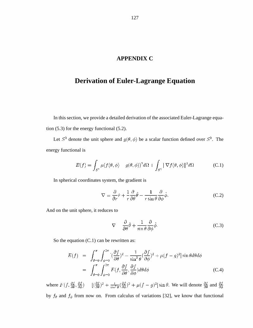
127

APPENDIX C

Derivation of Euler-Lagrange Equation

In this section, we provide a detailed derivation of the associated Euler-Lagrange equa-

tion (5.3) for the energy functional (5.2).

Let S2 denote the unit sphere andg(�; �) be a scalar function defined overS2. The

energy functional is

E(f) =

ZS2�(f(�; �)� g(�; �))2d +

ZS2krf(�; �)k2d (C.1)

In spherical coordinates system, the gradient is

r =@

@rr +

1

r

@

@�� +

1

r sin �

@

@��: (C.2)

And on the unit sphere, it reduces to

r =@

@�� +

1

sin �

@

@��: (C.3)

So the equation (C.1) can be rewritten as:

E(f) =

Z �

�=0

Z 2�

�=0

[(@f

@�)2 +

1

sin2 �(@f

@�)2 + �(f � g)2] sin �d�d�

=

Z �

�=0

Z 2�

�=0

F (f;@f

@�;@f

@�)d�d� (C.4)

whereF (f; @f@�; @f@�) = [(@f

@�)2 + 1

sin2 �(@f@�)2 + �(f � g)2] sin �. We will denote@f

@�and @f

@�

by f� andf� from now on. From calculus of variations [32], we know that functional

128

E is stationary if and only if its first variationÆE vanishes. We introduce an arbitrary

function�(�; �), which possesses a continuous second derivative and vanishes outside the

boundary. Let� be a parameter,

ÆE = �d

d�E(f + ��)

�����=0

(C.5)

This is equivalent to equation

ÆE = �

Z �

�=0

Z 2�

�=0

(Ff� + Ff��� + Ff���)d�d� (C.6)

By Gauss’s integral theorem and imposing the condition� = 0 on the boundary, we

obtain

ÆE = �

Z �

�=0

Z 2�

�=0

�

�Ff � @

@�Ff� �

@

@�Ff�

�d�d� (C.7)

The equationÆE = 0 must be valid for any arbitrary continuously differentiable func-

tion �. Therefore we can concludef(�; �) must satisfy the Euler-Lagrange differential

equation

Ff � @

@�Ff� �

@

@�Ff� = 0 (C.8)

Substitution ofF (f; f�; f�) = [(@f@�)2+ 1

sin2 �(@f@�)2+�(f�g)2] sin � into equation (C.8)

yields

Ff � @

@�Ff� �

@

@�Ff�

= 2� sin �(f � g)� 2@

@�(sin �

@f

@�)� 2

1

sin �

@2f

@�2

= 2 sin �

��(f � g)� 1

sin �

@

@�(sin �

@f

@�)� 1

sin2 �

@2f

@�2

�= 2 sin �

��(f � g)�r2f

�= 0 (C.9)

And this gives out the Euler-Lagrange equation (5.3),

r2f � �(f � g) = 0 (C.10)

BIBLIOGRAPHY

129

130

BIBLIOGRAPHY

[1] R. J. Adler,The Geometry of Random Fields, Wiley, 1981.

[2] A. Albano, “Representation of digitized contours in terms of conic arcs and straight-line segments,”Computer Graphics and Image Processing, vol. 3, , 1974.

[3] G. B. Arfken, Mathematical Methods For Physicists, Academic Press, Orlando, 3edition, 1985.

[4] G. Aubert and L. Blanc-F´eraud, “Some remarks on the equivalence between 2Dand 3D classical snakes and geodesic active contours,”International Journal ofComputer Vision, vol. 34, no. 1, pp. 19–28, 1999.

[5] N. Ayache, P. Cinquin, I. Cohen, L. Cohen, F. Leitner, and O. Monga, “Segmenta-tion of complex three-dimensional medical objects: a challenge and a requirementfor computer-assisted surgery planning and performance,” inComputer-IntegratedSurgery: Technology and Clinical Applications, pp. 59–74, MIT Press, 1996.

[6] L. Bers, F. John, and M. Schechiter,Partial Differential Equations, John Wiley andSons, 1964.

[7] J. A. K. Blokland, A. M. Vossepoel, A. R. Bakker, and E. K. J. Paulwels, “Delineat-ing elliptical objects with an application to cardiac scintigrams,”IEEE Transactionson Medical Imaging, vol. 6, no. 1, pp. 57–66, 1987.

[8] G. J. Boer and L. Steinberg, “Fourier series on sphere,”Atmosphere, vol. 13, pp.180, 1975.

[9] R. M. Bolle and B. C. Vemuri, “On three-dimensional surface reconstruction meth-ods,” IEEE Trans. on Pattern Analysis and Machine Intelligence, vol. 13, no. 1, pp.1–13, Jan. 1991.

[10] G. Bonneau, “Multiresolution analysis on irregular surface meshes,”IEEE Trans.on Visualization and Computer Graphics, vol. 4, no. 4, pp. 365–378, 1998.

[11] F. L. Bookstein, “Fitting conic sections to scattered data,”Computer Graphics andImage Processing, vol. 9, pp. 56–71, 1979.

131

[12] N. A. Borghese and S. Ferrari, “A portable modular system for automatic acquisi-tion of 3-D objects,”IEEE Trans. on Instrumentation and Measurement, vol. 49,no. 5, pp. 1128–1136, Oct. 2000.

[13] J. P. Boyd, “The choice of spectral functions on a sphere for boundary and eigen-value problems: A comparison of Chebyshev, Fourier and associated Legendre ex-pansions,”Monthly Weather Review, vol. 106, pp. 1184–1191, Aug. 1978.

[14] J. P. Boyd,Chebyshev and Fourier Spectral Methods, Springer-Verlag, New York,1989.

[15] C. Brechbuhler, G. Gerig, and O. K¨ubler, “Parametrization of closed surfaces for3-D shape description,”Computer Vision and Image Understanding, vol. 61, no. 2,pp. 154–170, March 1995.

[16] Y. Bresler and A. Macovski, “Three-dimensional reconstruction from projectionswith incomplete and noisy data by object estimation,”IEEE Transactions on Acous-tics Speech Signal Processing, vol. 35, pp. 1139–1152, 1987.

[17] L. G. Brown, “A survey of image registration techniques,”ACM Computing Sur-veys, vol. 24, no. 4, pp. 325–376, Dec. 1992.

[18] L. G. Brown, G. Q. Maguire, and M. E. Noz, “Landmark-based 3D fusion of SPECTand CT images,” inProceedings of the SPIE, Sensor Fusion VI, volume 2059, pp.166–174, 1993.

[19] G. Burel, “Three-dimensional invariants and their application to object recognition,”Signal Processing, vol. 45, pp. 1–22, 1995.

[20] G. Burel and H. Henocq, “Determination of the orientation of 3D objects usingspherical harmonics,”Graphical Models and Image Processing, vol. 57, no. 5, pp.400–408, 1995.

[21] V. Caselles, F. Catte, T. Coll, and F. Dibos, “A geometric model for active contours,”Numerische Mathematik, vol. 66, pp. 1–31, 1993.

[22] V. Caselles, R. Kimmel, and G. Sapiro, “Geodesic active contours,”InternationalJournal of Computer Vision, vol. 22, no. 1, pp. 61–79, 1997.

[23] T. F. Chan and L. A. Vese, “Active contours without edges,”IEEE Trans. on ImageProcessing, vol. 10, no. 2, pp. 266–277, Feb. 2001.

[24] P. Charbonnier, L. Blanc-F´eraud, A. G., and B. M., “Deterministic edge-preservingregularization in computed imaging,”IEEE Transactions on Image Processing, vol.6, no. 2, pp. 298–311, Feb. 1997.

[25] H. Cheong, “Double Fourier series on a sphere: Applications to elliptic and vorticityequations,”Journal of Computational Physics, vol. 157, no. 1, pp. 327–349, January2000.

132

[26] I. Cohen and L. D. Cohen, “Hyperquadric model for 2D and 3D data fitting,” inProceedings of the 12th IAPR International. Conference on Pattern Recognition,volume 2, pp. 403–405, 1994.

[27] L. D. Cohen and I. Cohen, “Finite-element methods for active contour models andballoons for 2-D and 3-D images,”IEEE Transactions on Pattern Analysis and Ma-chine Intelligence, vol. 15, no. 11, pp. 1131–1147, 1993.

[28] A. Collignon, F. Maes, D. Delaere, D. Vandermeulen, P. Suetens, and G. Marchal,Information Processing in Medical Imaging, chapter Automated Multi-modalityImage Registration Based On Information Theory, pp. 263–274, Kluwer Academic,Dordrecht, 1995.

[29] D. R. Cooper and N. Yalabik, “On the computational cost of approximating andrecognizing noise-perturbed straight lines and quadratic arcs in the plane,”IEEETrans. on Computers, vol. 25, , 1976.

[30] T. F. Cootes, C. J. Taylor, D. H. Cooper, and J. Graham, “Active shape models -their training and application,”Computer Vision and Image Understanding, vol. 61,no. 1, pp. 38–59, Jan. 1995.

[31] S. Cormier, N. Boujemaa, F. Tranquart, and L. Pourcelot, “Multimodal brain imagesregistration with severe pathological information missing,” inProceedings of theFirst Joint BMES/EMBS Conference, volume 2, pp. 13–16, Oct. 1999.

[32] R. Courant and D. Hilbert,Methods of Mathematical Physics, Interscience, 1953.

[33] C. A. Davatzikos and J. L. Prince, “An active contour model for mapping the cor-tex,” IEEE Trans. on Medical Imaging, vol. 14, pp. 65–80, 1995.

[34] D. DeCarlo and D. Metaxas, “Blended deformable models,”IEEE Transactions onPattern Analysis and Machine Intelligence, vol. 18, no. 4, pp. 443–448, April 1996.

[35] D. DeCarlo and D. Metaxas, “Shape evolution with structural and topologicalchanges using blending,”IEEE Transactions on Pattern Analysis and Machine In-telligence, vol. 20, no. 11, pp. 1186–1205, Nov. 1998.

[36] H. Delingette and J. Montagnat, “Topology and shape constraints on parametricactive contours,” Technical report, INRIA, France, 2000.

[37] P. Diaconis and D. Rockmore, “Efficient computation of the Fourier transform onfinite groups,”Journal of the American Mathematical Society, vol. 3, no. 2, pp.297–332, 1990.

[38] P. C. Doerschuk and J. E. Johnson, “Ab inito reconstruction and experimental designfor cryo electron microscopy,”IEEE Trans. on Information Theory, vol. 46, no. 5,pp. 1714–1729, Aug. 2000.

133

[39] J. R. Driscoll and D. M. Healy, “Computing Fourier transform and convolutions onthe 2-sphere,”Advances in Applied Mathematics, vol. 15, pp. 202–250, 1994.

[40] K. B. Eom, “Long-correlation image models for textures with circular and ellipticalcorrelation structures,”IEEE Trans. on Image Processing, vol. 10, no. 7, pp. 1047–1055, July 2001.

[41] S. Erturk and T. J. Dennis, “3D model representation using spherical harmonics,”Electronics Letters, vol. 33, no. 11, pp. 951–952, May 1997.

[42] O. Faugeras,Three-Dimensional Computer Vision, MIT Press, 1993.

[43] J. A. Fessler and A. O. Hero, “Penalized maximum-likelihood image reconstructionusing space-alternating generalized em algorithms,”IEEE Trans. on Image Process-ing, vol. 4, no. 10, pp. 1417–29, 1995.

[44] J. A. Fessler and A. Macovski, “Object-based 3-D reconstruction of arterial treesfrom magnetic resonance angiograms,”IEEE Transactions on Medical Imaging,vol. 10, no. 1, pp. 25–39, March 1991.

[45] A. F. Frangi, D. Rueckert, J. A. Schnabel, and W. J. Niessen, “Automatic 3D ASMconstruction via atlas-based landmarking and volumetirc elastic registration,” inProceedings of 17th International Conference of Information Processing in Med-ical Imaging, M. F. Insana and R. M. Leahy, editors, pp. 78–91, Davis, CA, USA,June 2001, Springer-Verlag.

[46] P. FunkMath. Ann., vol. 77, pp. 136–152, 1916.

[47] C. Giertsen, “Volume visualization of sparse irregular meshes,”IEEE ComputerGraphics and Applications, vol. 12, no. 2, pp. 40–48, Mar. 1992.

[48] R. Gnanadesikan,Methods for Statistical Data Analysis of Multivariate Observa-tions, Wiley, New York, 1977.

[49] A. Goshtasby, “Image registration by local approximation methods,”Image andVision Computing, vol. 6, no. 4, pp. 255–261, Nov. 1988.

[50] D. Gottlieb and S. A. Orszag,Numerical Analysis of Spectral Methods: Theory andApplications, Society for Industrial and Applied Mathematics, Philadelphia, 1977.

[51] A. Gray,Modern Differential Geometry of Curves and Surfaces with MATHEMAT-ICA, CRC Press, second edition, 1998.

[52] A. Gupta, T. O’Donnell, and A. Singh, “Segmentation and tracking of cine car-diac MR and CT images using a 3-D deformable models,” inProceedings of IEEEConference on Computers in Cardiology, 1994.

[53] P. Haigron, G. Lefaix, X. Riot, and R. Collorec, “Application of spherical harmonicsto the modelling of anatomical shapes,”Journal of Computing and InformationTechnology, vol. 6, no. 4, pp. 449–461, December 1998.

134

[54] S. Han, D. B. Goldgof, and K. W. Bowyer, “Using hyperquadrics for shape recov-ery from range data,” inIEEE Proceedings. Fourth International Conference onComputer Vision, pp. 492–496, 1993.

[55] D. M. Healy, D. N. Rockmore, and S. B. Moore, “An FFT for the 2-sphere andapplications,” inProceedings of International Conference on Acoustics, Speech,and Signal Processing, 1996.ICASSP-96, volume 3, pp. 1323–1326, Atlanta, GA,May 1996.

[56] E. HeckeMath. Ann, vol. 78, pp. 398–404, 1918.

[57] D. R. Hernandez,Lectures on Probability and Second Order Random Fields, WorldScientific, 1995.

[58] C. T. Ho and L. H. Chen, “A fast ellipse/circle detector using geometric symmetry,”Pattern Recognition, vol. 28, no. 1, pp. 117–124, 1995.

[59] E. W. Hobson,The Theory of Spherical and Ellipsoidal Harmonics, Cambridge,1931.

[60] R. J. Jaszczak, “Tomographic radiopharmaceutical imaging,”Proceedings of theIEEE, vol. 76, no. 9, pp. 1079–94, 1988.

[61] S. Jehan-Besson, M. Barlaud, and G. Aubert, “Video object segmentation usingEulerian region-based active contours,” inProceedings Eighth IEEE InternationalConference on Computer Vision, volume 1, pp. 353–60, Vancouver, BC, Canada,July 2001.

[62] K. Kanatani, “Analysis of 3-D rotation fitting,”IEEE Transactions on Pattern Anal-ysis and Machine Intelligence, vol. 16, pp. 543–549, 1994.

[63] M. Kass, A. Witkin, and D. Terzopoulos, “Snakes: Active contour models,”Inter-national Journal of Computer Vision, vol. 1, no. 4, pp. 321–331, 1987.

[64] T. Kayikcioglu, A. Gangal, and M. Ozer, “Reconstructing ellipsoids from threeprojection contours,”Pattern Recognition Letters, vol. 21, pp. 959–968, 2000.

[65] V. S. Khoo, D. P. Dearnaley, D. J. Finnigan, A. Padhani, S. F. Tanner, and M. O.Leach, “Magnetic resonance imaging (MRI): considerations and applications in ra-diotherapy treatment planning,”Radiotherapy and Oncology, vol. 42, no. 1, pp.1–15, 1997.

[66] B. B. Kimia, A. R. Tannenbaum, and S. W. Zucker, “Shapes, shocks, and defor-mations I: The components of two-dimensional shape and the reaction-diffusionspace,”International Journal of Computer Vision, vol. 15, no. 3, pp. 189–224, 1995.

135

[67] K. F. Koral, Y. Dewaraja, L. A. Clarke, J. Li, K. R. Zasadny, and S. G. Rom-melfanger, “Tumor absorbed dose estimates versus response in tositumomab ther-apy of previously-untreated patients with follicular non-Hodgkin’s lymphoma: pre-liminary report,”Cancer Biotherapy and Radiopharmaceuticals, vol. 15, no. 4, pp.347–355, 2000.

[68] K. F. Koral, Y. Dewaraja, J. Li, S. Lin, C. L. Barrett, and D. D. Regan, “Initial re-sults for hybrid SPECT-conjugate-view tumor dosimetry in I-131 anti-B1-antibodytherapy of previously-untreated lymphoma patients,”Journal of Nuclear Medicine,vol. 41, no. 9, pp. 1579–1586, 2000.

[69] E. L. Kramer, M. E. Noz, J. J. Samger, A. J. Megibow, and G. Q. Maquire, “CT-SPECT fusion to correlate radiolabeled monoclonal antibody uptake with abdomi-nal CT findings,”Radiology, vol. 172, pp. 861–865, 1989.

[70] D. J. Kriegman and J. Ponce, “On recognizing and positioning curved 3-D objectsfrom image contours,”IEEE Transactions on Pattern Analysis and Machine Intelli-gence, vol. 12, no. 12, pp. 1127–1137, 1990.

[71] M. E. Leventon, W. E. L. Grimson, and O. Faugeras, “Statistical shape influencein geodesic active contours,” inProceedings IEEE Conference on Computer Visionand Pattern Recognition, volume 1, pp. 316–323, Jun. 2000.

[72] L. Liu, P. H. Bland, D. M. Williams, B. G. Schunck, and C. R. Meyer, “Applicationof robust sequential edge detection and linking to boundaries of low contrast lesionsin medical images,” inProceedings CVPR ’89, pp. 582–587, 1989.

[73] X. Lv, J. Zhou, and C. Zhang, “A novel algorithm for rotated human face detec-tion,” in Proceedings IEEE Conference on Computer Vision and Pattern Recogni-tion. CVPR 2000, volume 1, pp. 13–15, June 2000.

[74] G. Q. Maguire, M. E. Noz, H. Rusinek, J. Jaeger, E. L. Kramer, J. J. Sanger,and G. Smith, “Graphics applied to medical image registration,”IEEE ComputerGraphics and Applications, vol. 11, no. 2, pp. 20–8, 1991.

[75] R. Malladi, J. Sethian, and B. Vemuri, “Shape modelling with front propagation: Alevel set approach,”IEEE Trans. on Pattern Analysis and Machine Intelligence, vol.17, no. 2, pp. 158–174, 1995.

[76] A. Matheny and D. B. Goldgof, “The use of three and four dimensional surfaceharmonics for rigid and nonrigid shape recovery and representation,”IEEE Trans-actions on Pattern Analysis and Machine Intelligence, vol. 17, no. 10, pp. 967–981,Oct. 1995.

[77] T. McInerney and D. Terzopoulos, “Deformable models in medical image analysis,”in Proceedings of the IEEE Workshop on Mathematical Methods in BiomedicalImage Analysis, pp. 171–180, San Francisco, CA, USA, June 1996.

136

[78] T. McInerney and D. Terzopoulos, “Topology adaptive deformable surfaces formedical image volume segmentation,”IEEE Transactions on Medical Imaging, vol.18, no. 10, pp. 840–850, Oct. 1999.

[79] M. Merickel, “3D reconstruction: the registration problem,”Computer Vision,Graphics, and Image Processing, vol. 42, no. 2, pp. 206–219, 1988.

[80] C. R. Meyer, J. L. Boes, B. Kim, P. H. Bland, K. R. Zasadny, P. V. Kison, K. F. Koral,K. A. Frey, and R. L. Wahl, “Demonstration of accuracy and clinical versatility ofmutual information for automatic multimodality image fusion using affine and thin-plate spline warped geometric deformations,”Medical Image Analysis, vol. 1, no.3, pp. 195–206, Apr. 1997.

[81] D. Mumford and J. Shah, “Optimal approximation by piecewise smooth functionsand associated variational problems,”Communications on pure and applied mathe-matics, vol. 42, pp. 577–685, 1989.

[82] A. F. Nikiforov, S. K. Suslov, and V. B. Uvarov,Classical Orthogonal Polynomialsof a Discrete Variable, Springer-Verlag, 1991.

[83] S. A. Orszag, “Fourier series on spheres,”Monthly Weather Review, vol. 102, pp.56–75, 1974.

[84] S. J. Osher and J. A. Sethian, “Fronts propagation with curvature dependent speed:Algorithms based on Hamilton-Jacobi formulations,”Journal of ComputationalPhysics, vol. 79, pp. 12–49, 1988.

[85] K. A. Paton, “Conic sections in chromosome analysis,”Pattern Recognition, vol. 2,, 1970.

[86] E. Persoon and K. S. Fu, “Shape discrimination using Fourier descriptors,”IEEETransactions on Pattern Analysis and Machine Intelligence, vol. 8, no. 3, pp. 388–397, May 1986.

[87] R. Piramuthu,Robust Fusion of MRI and ECT Data, and Acceleration of EM Al-gorithm Using Proximal Point Approach, PhD thesis, The Univ. of Michigan, AnnArbor, May 2000.

[88] W. H. Press, B. P. Flannery, S. A. Teukolsky, and W. T. Vetterling,NumericalRecipes in C: The Art of Scientific Computing, Cambridge University Press, 1988.

[89] D. Rockmore, “Computation of Fourier transforms on the symmetric group,” inComputers and mathematics, pp. 156–165, Springer, 1989.

[90] C. Scarfone. Single Photon Emission Computed Tomography.http://www.bae.ncsu.edu/bae/course/bae590f/1995/scarfone, 1995.

[91] M. D. Srinath,Introduction to Statistical Signal Processing with Applications, Pren-tice Hall, 1996.

137

[92] L. H. Staib and J. S. Duncan, “Parametrically deformable contour model,” inPro-ceedings IEEE Conference on Computer Vision and Pattern Recognition (CVPR),pp. 98–103, 1989.

[93] L. H. Staib and J. S. Duncan, “Model-based deformable surface finding for medicalimages,”IEEE Transactions on Pattern Analysis and Machine Intelligence, vol. 15,no. 5, pp. 1996, Oct. 1996.

[94] H. Stark and J. W. Woods,Probability, Random Processes, and Estimation Theoryfor Engineers, Prentice Hall, second edition, 1994.

[95] P. Taylor, “Invited review: computer aids for decision-making in diagnostic radiol-ogy - a literature review,”British Journal of Radiology, vol. 68, pp. 945–957, 1995.

[96] D. Terzopoulos and D. Metaxas, “Dynamic 3D models with local and global defor-mations: Deformable superquadrics,”IEEE Transactions on Pattern Analysis andMachine Intelligence, vol. 13, no. 9, pp. 703–714, July 1991.

[97] S. R. Titus,Improved Penalized Likelihood Reconstruction of Anatomically Corre-lated Emission Computed Tomography Data, PhD thesis, The Univ. of Michigan,Ann Arbor, Dec. 1996.

[98] Unknown, editor,Mathematics Handbook, China Science Publisher, 1992.

[99] B. C. Vemuri and Y. Guo, “Snake pedals: Compact and versatile geometric modelswith physics-based control,”IEEE Transactions on Pattern Analysis and MachineIntelligence, vol. 22, no. 5, pp. 445–459, May 2000.

[100] P. Viola and W. M. Wells III, “Alignment by maximization of mutual information,”in Proceedings of IEEE International Conference on Computer Vision, pp. 16–23,Los Alamitos, CA, Jun. 1995.

[101] R. G. Voigt, D. Gottlieb, and M. Y. Hussaini,Spectral Methods for Partial Dif-ferential Equations, Society for Industrial and Applied Mathematics, Philadelphia,1984.

[102] D. H. Von Seggern,PHB practical handbook of curve design and generation, CRCPress, 1994.

[103] Y. Wang and L. H. Staib, “Elastic model based non-rigid registration incorporatingstatistical shape information,” inMedical Image Computing and Computer AidedIntervention, pp. 1162–1173. Springer, 1998.

[104] E. T. Whittaker,A course of modern analysis; an introduction to the general theoryof infinite processes and of analytic functions; with an account of the principaltranscendental functions, Cambridge The university Press, 1950.

[105] E. Wigner,Group Theory and its Application to Quantum Mechanics of AtomicSpectra, Academic Press, New York, 1959.

138

[106] W. Y. Wu and M. J. J. Wang, “Elliptical detection by using its geometric properties,”Pattern Recognition, vol. 26, no. 10, pp. 1499–1509, 1993.

[107] C. Xu, Deformable Models With Application to Human Cerebral Cortex Recon-struction from Magnetic Resonance Images, PhD thesis, The Johns Hopkins Uni-versity, 2000.

[108] C. Xu and J. L. Prince, “Snakes, shapes, and gradient vector flow,”IEEE Trans. onImage Processing, vol. 7, no. 3, pp. 359–369, March 1998.

[109] C. Xu, A. Yezzi, and J. L. Prince, “On the relationship between parametric and ge-ometric active contours,” Technical Report ECE 99-14, Johns Hopkins University,Dec. 1999.

[110] M. I. Yadrenko,Spectral theory of random fields, Optimization Software, 1983.

[111] S. Y. K. Yee, “Studies on Fourier series on spheres,”Monthly Weather Review, vol.108, pp. 676–678, 1980.

[112] S. Y. K. Yee, “Solution of Poisson’s equation on a sphere by truncated doubleFourier series,”Monthly Weather Review, vol. 109, pp. 501–505, 1981.

[113] R. K. K. Yip, K. S. Tam, and D. N. K. Leung, “Modification of hough transformfor circles and ellipses detection using a 2-dimensional array,”Pattern Recognition,vol. 25, no. 9, pp. 1007–1022, 1992.

[114] A. C. Zaanen,Linear Analysis, North Holland, 1956.

[115] Y. Zhang, M. Brady, and S. Smith, “Segmentation of brain MR images through ahidden markov random field model and the expectation-maximization algorithm,”IEEE Trans. on Medical Imaging, vol. 20, no. 1, pp. 45–57, Jan. 2001.

[116] S. C. Zhu, Y. Wu, and D. Mumford, “Filters, random fields and maximum entropy(frame): Towards a unified theory for texture modeling,”International Journal ofComputer Vision, vol. 27, no. 2, pp. 107–126, 1998.