ARL-TR-2878 DECEMBER 2002

Three-Dimensional Stereo Reconstruction andSensor Registration With Application to the

Development of a Multi-Sensor Database

William F. OberleGary A. Haas

ARMY RESEARCH LABORATORY

Approved for public release; distribution is unlimited.

NOTICES

Disclaimers

The findings in this report are not to be construed as an officialDepartment of the Army position unless so designated by otherauthorized documents.

Citation of manufacturers’ or trade names does not constitute an officialendorsement or approval of the use thereof.

DESTRUCTION NOTICEDestroy this report when it is no longerneeded. Do not return it to the originator.

i

Army Research LaboratoryAberdeen Proving Ground, MD 21005-5066____________________________________________________________________________

ARL-TR-2878 December 2002____________________________________________________________________________

Three-Dimensional Stereo Reconstruction and SensorRegistration With Application to the Development of aMulti-Sensor Database

William F. Oberle and Gary A. HaasWeapons and Materials Research Directorate

____________________________________________________________________________

Approved for public release; distribution is unlimited.____________________________________________________________________________

ii

ACKNOWLEDGMENTS

The authors would like to thank Raymond Von Wahlde of the U.S. Army Research Laboratoryfor his time and effort in reviewing this report. His comments and observations are greatlyappreciated.

iii

Contents

1. Introduction .............................................. 1

2. Registration Between a Single Camera and the Calibration System ..... 2

2.1 Step 1 ................................................ 22.2 Step 2 ................................................ 4

3. Registration of Stereo Cameras................................ 10

4. Three-Dimensional Reconstruction ............................. 12

5. Registration of Sensor Systems ................................ 15

6. Application to a Multi-Sensor Database.......................... 16

7. Summary ................................................ 23

References .................................................... 25

AppendixA. C++ Program to Perform 3-D Reconstruction....................... 27B. Three-Dimensional Reconstruction for Stereo Data Used in Stereo-LADAR Registration, Based on Results of Program of Appendix A ............... 31C. Results of LADAR 3-D Reconstruction With NIST Procedure Data Used in Stereo-LADAR Registration .................................. 35

Report Documentation Page........................................ 37

iv

Figures

1. ARL calibration facility poster in the left rear station .................... 3 2. Schematic of the calibration and camera coordinate systems ................ 5 3. Left camera images of the calibration poster, clockwise, left rear, right rear,

right front, and left front....................................... 8 4. Error (multipled by 100) between sensed location of calibration circles and

projected location of circles with the camera model...................... 9 5. The data sources for the registration ............................... 17 6. Pixel locations of target in left and right camera together with the result of 3-D

reconstruction .............................................. 17 7. Schematic of location (distance relative to camera reference frame) and

orientation of targets ......................................... 18 8. Effect on y-coordinate because of tilted coordinate system ................. 19 9. Transformed stereo points to LADAR coordinate system.................. 2010. Overlay of transformed stereo and LADAR points, LADAR coordinate system.... 2011. Error associated with the stereo-LADAR registration..................... 23

Table

1. Statistics from the comparison .................................. 22

1

THREE-DIMENSIONAL STEREO RECONSTRUCTION AND SENSOR REGISTRATION WITH APPLICATION TO THE DEVELOPMENT OF A MULTI-SENSOR DATABASE

1. Introduction

During the past several decades, unmanned ground vehicle (UGV) technology has progressed from tethered teleoperated vehicles to vehicles capable of autonomous movement through off-road terrain. Keys to this success in the area of autonomous mobility have been the increased computational capacity available to the vehicle, software architectures specifically designed for UGV applications (e.g., four-dimensional real-time control system [Albus, 1997] by the National Institute of Standards [NIST]), and improved sensor technology for obstacle avoidance, especially in laser radar (LADAR). The extension of UGV functionality to application areas of interest to the Army besides autonomous mobility will most likely require the improvement and integration of a number of sensor technologies. Besides LADAR, other technologies include infrared (IR) sensors and monocular or binocular imagery. The integration or fusion of the data provided by all the vehicle’s sensors will be necessary to exploit the potential benefits offered by UGVs for Army applications.

A necessary condition for the fusion of sensor data is the capability of reconciling the individual coordinate systems or reference frames associated with the various sensors, vehicles, and the world. Specifically, this requires knowledge of the transformations (rigid body rotation plus translation) among the different coordinate systems.

The Weapons Analysis Branch, Ballistics and Weapons Concepts Division, Weapons and Materials Research Directorate of the U.S. Army Research Laboratory (ARL) has undertaken a research effort in robotic perception, which focuses on binocular or stereoscopic vision. This effort includes a collaborative effort with NIST to develop a multi-sensor (LADAR, navigation [NAV], and stereoscopic video [stereo]) database with ground truth

1 for use by the robotics

research community. As described in the previous paragraph, for these data to be useful, the transformations among the various sensor coordinate systems must also be provided. The objective of this report is to document the ARL procedure for determining the transformations among the cameras of the stereo system and the transformations among the camera system and other sensor, vehicle, and world coordinate systems. In this report, the process of determining a transformation between two coordinate systems is referred to as registration. Essentially, the registration process between two sensor coordinate systems requires knowledge of the three-dimensional (3-D) coordinates in each sensor coordinate system for a number of corresponding points. Thus, the problem is not only sensor registration but also, in the case of the stereo system

1An accurate positional location determined by direct measurement or survey.

2

data, 3-D reconstruction. Data from the stereo system consist of two-dimensional (2-D) images. Three-dimensional reconstruction refers to the process of merging this 2-D information, measured at pixel locations in the two camera images, to retrieve 3-D coordinates for features observed in both images. As described next, ARL’s procedure entails the use of software developed by the Jet Propulsion Laboratory (JPL), computer code written by ARL, and a MATLAB

2 routine.

The organization of the remainder of the report is as follows. Registration of a single camera and the calibration system is covered in Section 2. Section 3 describes the registration between the stereo cameras. Three-dimensional reconstruction of the stereo images is described in Section 4. Registration between the stereo system and other sensor systems is presented in Section 5. The application of this work to the development of a multi-sensor database is described in Section 6. Finally, a summary of this work is presented in Section 7.

2. Registration Between a Single Camera and the Calibration System

As discussed, the goal of registration is to determine the rigid body transformation relating two coordinate systems. Specifically, this entails determining a translation vector T and a rotation matrix R that convert the coordinates P1 of a point in the first coordinate system to the coordi-nates P2 of that same point in the second coordinate system. The relation between P1 and P2 is given by

P2 = R * (P1 - T). (1) The registration procedure involving a single camera and the calibration system used by ARL is performed in two steps. First is the determination of a camera model via software and a procedure adopted from JPL. Step 2 converts the information from the camera model of Step 1 into the desired rotation and translation. Both steps are described next. Since ARL is interested in stereoscopic video, the data necessary to determine the individual camera model for each of the two cameras are collected and processed during Step 1. Thus, the discussion of Step 1 refers to a pair of cameras.

2.1 Step 1

The cameras are fixed in a stereo “rig,” a fixture that maintains a rigid body geometry between the two and defines the binocular stereo pair. The cameras provide input to personal computer frame “grabber” boards that digitize and store the images from the camera pair. These images are of a highly structured calibration scene and are recorded and processed off line by the JPL

2MATLAB® is a registered trademark of The MathWorks.

3

calibration software (Litwin, 2000). An explicit model of each camera is calculated on the basis of surveyed 3-D points in the calibration scene and the corresponding 2-D points in the camera image.

ARL’s calibration facility, which was designed, built, and based on performance specifications provided by Larry Matthies of JPL

3, provides a source of 3-D points. The locations of these 3-D

points are precisely known. A typical calibration uses four binocular images of a calibration “poster,” shown in Figure 1. An image is taken of the poster at each of four surveyed poster stations (left front, right front, left rear, and right rear) within the field of view of the stereo rig.

Figure 1. ARL calibration facility poster in the left rear station. (Floor plates for the right rear station can also be seen.)

The aluminum poster has 150 white circular markings on a black background, each machined by an ARL computer numerically controlled (CNC) milling machine to a nominal spacing accuracy better than 0.127 mm (0.005 inch). Spacing of the 41.91-mm (1.650-inch) diameter circles is 81.28 mm (3.200 inches) between centers. The white-on-black circles provide a high contrast image, and CNC accuracy assures regularity of spacing within the poster.

The poster is mounted on a rigid aluminum stand. It holds the poster at a precisely measured location in space in one of the four poster stations. Each poster station consists of three machined stainless steel floor plates bolted to the concrete floor of the facility. The geometry of the

3Private communication, Larry Matthies, Jet Propulsion Laboratory, California Institute of Technology, Pasadena,

California, 1997.

4

machined stainless steel feet of the poster stand constrains the stand in exactly 6 degrees of freedom, so there is only one stable way for the stand to sit on the floor plates. The location of the poster has been surveyed in each of the four stations by a high accuracy instrument, based on laser tracking technology. An arbitrary coordinate system fixed to the calibration facility is used. Several repetitions of the survey indicate that when the poster is in a station, the location of each circle is known to within an accuracy of less than 0.05 mm (i.e., a few thousandths of an inch).

The stored images are processed off line with the JPL calibration software, separately for each camera. The images of the calibration poster in each of its four stations are used as input to the JPL software in combination with data files that provide the 3-D coordinates, relative to the reference frame of the calibration system, of the corner elements of the poster in each station. Additionally, a nominal set of values for the camera intrinsic parameters (Trucco & Verri, 1998) is entered in the program. The JPL software incorporates an algorithm described by Gennery, Litwin, Wilcox, and Bon (1987), which detects the centers of the circles in the four images from each camera and correlates the results with the known locations of the centers. Intrinsic and extrinsic parameters of the camera are extracted and tested. The software yields a camera model in the CAHVOR4

format described in Yakimovsky and Cunningham (1978) and Gennery (2001), along with circle location error analysis information. The intrinsic and extrinsic parameters are required in Step 2 to complete the calibration system-camera registration. Details about these parameters are provided in Step 2.

2.2 Step 2

The extrinsic parameters determined by the JPL software in the CAHVOR format include four vectors C, A, H, and V. The vector C, shown in Figure 2, represents the translation vector associated with the rigid body transformation from the calibration coordinate system to the camera coordinate system. Therefore, if T is the translation vector of the rigid body transfor-mation,

T = C. (2) Assuming no lens distortion, A is a unit vector along the focal axis of the camera, and H and V satisfy the equations (Yakimovsky & Cunningham, 1978):

i P C HP C A

j P C VP C A

=−−

=−−

( , )( , )

( , )( , )

and . (3)

The vectors H and V are not necessarily orthogonal to the vector A nor parallel to the x- or y-axis of the camera coordinate system. H contains information relative to the horizontal direction and V information relative to the vertical direction. The vector H is the sum of vectors, one in the direction of the camera x-axis and the other along A. A similar definition applies to V but

4Not an acronym

5

with the first vector in the camera y-axis direction. The definitions for H and V are chosen to simplify the calculation of i and j, as given in Equation (3) (JPL, 2002). As shown in Figure 2, (i,j) is the point in the image plane (pixel units relative to the camera image

5) associated with the

image of the point P (given in the calibration coordinate system). The superscript T represents the transpose of the vector or matrix and (.,.) the standard scalar or dot product of two vectors.

Figure 2. Schematic of the calibration and camera coordinate systems.

5In the image, the upper left-hand corner has pixel coordinates (0,0). The x-coordinate indicates the column number

and is positive to the right; the y-coordinate indicates the row number and is positive downward.

nn

n

Image PlaneCenter of Image

Plane (Ox,Oy) in pixels

Pixel Location (0,0)

Camera Coordinate System

World (Calibration) Coordinate System (WCS)

x

x

y

y

z

z

Focal or Optical Axis

Arbitrary Point P (WCS)

[x y z]T in CCS

Image of Point P (i,j) in pixels

[xim yim f]T in CCS

CC

PP

AA

PP -- CC

6

The next step is to determine the rotation matrix, R. Let [x y z]T represent the coordinates of the point P in the coordinate system of the camera; then, since A is a unit vector in the direction of the focal axis which corresponds to the z-axis of the camera coordinate system:

z = (P – C, A). (4) If R represents the rotation associated with the rigid body transformation between the calibration and camera coordinate systems, then the following relation between [x y z]T and P exists:

[x y z]T = R * (P – T), (5) or

[x y z]T = [ (R1T, P – T) (R2

T, P – T) (R3T, P – T) ]T (6)

in which Rk, k = 1, 2, 3, is the kth row of R. Therefore, from Equations (4) and (6),

(P – C, A) = (R3T, P – T). (7)

From Equation (1), T = C, and combined with the commutative property of the scalar product, it can be concluded from Equation (7) that

R3T = A. (8)

It now remains to determine R1 and R2. If [xim yim f]T is the image point of [x y z]T in the image plane relative to the camera coordinate system, then from Trucco and Verri (1998),

xim = (i – Ox) * sx and yim = (j – Oy) * sy. (9) (Ox,Oy) are the coordinates (in pixels) of the image center (i.e., intersection of the focal axis with the image plane) and (sx,sy) the effective size of a pixel (in millimeters) in the horizontal and vertical directions, respectively, and are provided as part of the intrinsic parameters from Step 1.

6

When Equation (9) is combined with the fundamental equation for a perspective camera (Trucco & Verri, 1998),

xim = f * x / z and yim = f * y / z, (10) in which f is the focal length of the camera, and it can be concluded that

(i – Ox) * sx = f * x / z and (j – Oy) * sy = f * y / z. (11) Substituting from Equation (6),

(i – Ox) * sx = f * (R1T, P – T)/ (R3

T, P – T) (12)

6The intrinsic parameters from Step 1 actually provide the ratios f/sx and f/sy; f is the focal length of the camera. As

will be seen, these ratios are needed.

7

and (j – Oy) * sy = f * (R2T, P – T)/ (R3

T, P – T). Rearranging the first equation in (12),

i * (R3T, P – T) = Ox * (R3

T, P – T) + (f / sx) * (R1T, P – T). (13)

Substituting for i from Equation (3),

(P– C, H)/(P– C, A) * (R3T, P– T) = Ox * (R3

T, P – T) + (f /sx) * (R1T, P– T). (14)

With Equation (8), the commutative property of the scalar product, and the fact that T = C, Equation (14) can be rewritten as

(H, P – T) = Ox * (R3T, P – T) + (f /sx) * (R1

T, P– T). (15) Solving for R1

T,

R1T = (sx / f) * ( H – Ox * R3

T ). (16) In like manner,

R2T = (sy / f) * ( V – Oy * R3

T ). (17) Since (Ox,Oy), f/sx, f/sy, H, V, and R3

T are known from the calibration camera model and Equation (8), R1

T and R2T can be determined. This completes the construction of the rotation

matrix R and Step 2.

To illustrate and validate the registration technique, data collected during a calibration experi-ment are used. Validating the registration entails obtaining the rigid body transformation (rotation matrix and translation vector) and then demonstrating that a point(s) expressed in the coordinate system of one of the reference frames is transformed into the correct coordinates in the second reference frame when the rigid body transformation is applied. As discussed before, a number of locations in the coordinate system of the calibration system have been accurately measured. However, the coordinates of these points, relative to the coordinate system of the camera, are not measured during the calibration. The only information with respect to these points relative to the camera reference frame is their pixel location in the image plane. Thus, the validation of the registration between the calibration system and the camera is to demonstrate that given a point(s) in the coordinate system of the calibration system, after the rigid body transformation is applied, the resulting pixel location in the image plane of the camera agrees with the measured pixel location. This extra step of converting from the 3-D coordinates in the coordinate system of the camera obtained from Equation (5)

7 to the pixel location in the image

employs Equation (11). Equation (11) involves the intrinsic parameters of the camera that are 7If the 3-D coordinates were available in the camera coordinate system, then the validation would be complete at this

point since Equation (5) provides the desired coordinates in the reference frame of the camera.

8

also provided by the JPL CAHVOR camera model. Although this would appear to introduce four independent parameters, Ox, Oy, f/sx, and f/sy, which could influence the pixel location results and question the correctness of the calculated rigid body transformation, this is not the case. The four intrinsic parameters are functions of the vectors A, H, and V, as is the rigid body transformation.

8

Figure 3. Left camera images of the calibration poster, clockwise, left rear, right rear, right front, and left front.

From the survey of the calibration fixture, the coordinates of the lower left corner of the calibra-tion poster in the left front position in the calibration system coordinate system are [-0.133933 –0.1286 –32.7774]T (units in inches

9). This point is denoted by PW1. The image of PW1 in the left

camera image plane has pixel coordinates (201, 223) and is denoted by pL1.10

Figure 3 shows the four left camera images used as input by the JPL calibration software in determining the intrinsic and extrinsic parameters of the camera. As discussed earlier, the program performs a number of iterations to minimize error in computing the intrinsic and extrinsic parameters. Figure 4 shows a display of the error analysis for the calibration. For

8Private communication, Adnar Ansar, Jet Propulsion Laboratory, California Institute of Technology, Pasadena, CA,

May 2002. 9All the information provided by the JPL calibration code is in units of inches. In order to use the exact output from

the JPL code in this report, English instead of metric units are used in the illustrations. 10

Lower case p denotes a location in the camera image plane. In Sections 2 and 3, the notation is used to denote an ordered pair corresponding to pixel locations. For Section 4, p represents a 3-D vector corresponding to a location in the camera image plane in the camera coordinate system.

9

the calibration shown, the maximum error is less than 0.5 pixel, and the root mean square (rms) error is less than 0.2 pixel.

Figure 4. Error (multiplied by 100) between sensed location of calibration circles and projected location of circles with the camera model.

The intrinsic and extrinsic information computed for the left camera with the JPL calibration software is

C = [-162.156653 21.75404 –49.475802]T, A = [0.991064 0.043105 0.126228]T, H = [312.74723 882.825431 54.525783]T, V = [129.686323 –2.725906 891.240401]T,

f/sx = 868.457302, f/sy = 867.812235, Ox = 354.889486, and Oy = 240.909425.

With Equations (8), (16), and (17), the rotation matrix for the left camera is computed to be

RL =F

HGG

I

KJJ

-0.044874 0.99893 0.011202-0.125684 - 0.015107 0.991955 0.991061 0.043105 0.126228

and TL = [-162.156653 21.75404 –49.475802]T with Equation (2).

Note that RL has the correct form to rotate the coordinate system of the calibration system to that of the camera. The first column of RL corresponds to the x-axis in the calibration system, and the location of the largest value in the column corresponds to the axis to which the x-axis is rotated in the camera coordinate system, specifically, the third row that corresponds to the z-axis.

10

Similarly, the y-axis (calibration) corresponds to the x-axis (camera), and the z-axis (calibration) corresponds to the y-axis (camera). Referring to Figure 2, it can be seen that this correspondence is correct. Also, if RL is a rotation matrix, it must be an orthogonal matrix (i.e., RT = R-1). The product of RL and RL

T is

R RL LT∗ =F

HGG

I

KJJ

1.0000003 0.0016609 - 0.0000001 0.0016609 0.9999994 0.0000004-0.0000001 0.0000004 0.9999994

,

which, considering numerical accuracy, can be considered equivalent to the required identity matrix. Thus, RL

T = RL-1 and RL is an orthogonal matrix.

Next, RL and TL together with PW1 are substituted into Equation (5) to determine the 3-D coordi-nates of PW1 in the coordinate system of the camera (refer to this point as PL1). The result is

PL1 = [x y z]T = [-28.942778 –3.469019 161.73944]T. Finally, with Equation (11) and the values of x, y, and z from PL1, the predicted pixel location in the left camera image plane is calculated to be

i = 199.5 and j = 222.3. Compared to the measured pixel location pL1 = (201, 223), the percentage error in the computed horizontal pixel location is –0.75% ([199.5 – 201]/201 * 100) and –0.31% ([222.3 – 223]/223 * 100) in the computed vertical pixel location.

Based on these results, the approach described in this section appears to correctly compute the rigid body transformation for the registration between the ARL calibration system and a single camera.

3. Registration of Stereo Cameras

Since both cameras used in the stereo pair must be calibrated relative to the calibration system before use, the registration between the cameras can be accomplished with the registration information between the calibration system and each camera. Let P, PL, and PR, represent the 3-D coordinates of the same point relative to the calibration system, left camera, and right camera coordinate systems, respectively. With the registration procedure described in Section 2, two rotational matrices, RL and RR, and two translation vectors, TL and TR, can be obtained, thereby registering the calibration system and the left and right cameras so that

PL = RL*(P – TL) and PR = RR*(P – TR). (18)

11

Solving the second equation in (18) for P and substituting into the first equation in (18),

PL = RL*( RRT * PR + TR – TL) = RL* RR

T * PR + RL * (TR – TL). (19) In general, for a stereo-video system, results are relative to the left camera. Thus, it is customary to express the rigid body transformation as transforming coordinates relative to the left camera coordinate system to coordinates relative to the right camera coordinate system. Rewriting Equation (19) to express the transformation in this manner yields

PR = (RL * RRT)T * [PL - RL* (TR - TL)]. (20)

Let RLR and TLR represent the rotation and translation from the left camera reference frame to the right camera reference frame. Then Equation (20) is rewritten in the form of Equation (1),

PR = RLR * (PL – TLR) with RLR = RR * RLT and TLR = RL * (TR – TL). (21)

Validation of the registration defined by Equation (21) between the cameras should be performed with the pixel location in the left and right camera images of the same point in space since the only measured information from the cameras is the camera image as discussed in Section 2. However, the rigid body transformation cannot be applied directly to the pixel locations but only to 3-D coordinates. As stated in Section 2, the point PW1 corresponds to the pixel location pL1 = (201, 223) in the left camera image and is approximately the 3-D location PL1 = [-28.942778 –3.469019 161.73944]. Analysis of the image from the right camera indicates that the point PW1 corresponds to the pixel location pR1 = (143, 217) in the right camera image plane. To validate the registration, Equation (21) is used with the point PL1 to estimate the 3-D location of PW1 in the coordinate system of the right camera. This point is denoted by PR1. Then Equation (11) is used to compute the predicted pixel location of PW1 in the right camera image plane. This pixel location is then compared to the measured pixel location pR1.

With the approach in Section 2, the intrinsic and extrinsic parameters determined by the JPL stereo code for the right camera are

C = [-162.973831 35.421890 –49.624169]T, A = [0.988809 0.018624 0.14802]T, H = [318.316874 846.307617 56.404557]T, V = [124.237891 –3.221699 868.448511]T, and

f/sx = 840.187051, f/sy = 840.522937, Ox = 338.864882, and Oy = 251.335317.

The resulting rigid body transformation is defined by

12

PR =F

HGG

I

KJJ

-0.019943 0.999773 0.007434-0.147866 - 0.009402 0.988963 0.988809 0.018624 0.14802

and TR = [-162.973831 35.42189 -49.624169]T. Substituting into Equation (21),

RLR =F

HGG

I

KJJ

0.999681 - 0.005223 0.024269 0.008322 0.999733 - 0.022115-0.02411 0.02227 0.99946

and TLR = [13.688233439 -0.250947397683 -0.239451102362]T. Thus,

PR1 = RLR * (PL1 – TLR) = [-38.6695384502 -7.15415083112 162.847589732]T. With Equation (11), the pixel location in the right camera image plane is calculated to be I = 139.4 and j = 214.4. Compared to pR1 = (143, 217), this represents a percentage error of approximately –2.5% in the horizontal pixel location and –1.2% in the vertical pixel location.

11

However, this includes propagation of the error included in PL1. From the previous section, the percentage error in the horizontal pixel direction of pL1 (an indication of the error in PL1) was -0.75% and in the vertical direction, –0.31%. Given the potential error propagation from the use of PL1, the fact that the pixel location for pR1 is selected by the user and because of possible numerical approximations, it is felt that the results for pR1 are sufficiently close to justify the conclusion that the registration between the two cameras is correctly represented by the results given in Equation (21).

4. Three-Dimensional Reconstruction

The process of 3-D reconstruction refers to determining the 3-D coordinates (relative to a given coordinate system) of points in the world, given two slightly different 2-D video images of the points. Of interest in this report is the configuration of cameras as a stereo pair, which provides the two images simultaneously. By selecting corresponding or conjugate points in the left and right camera images, one can determine the 3-D coordinates of the location of the appropriate point in space by triangulation. The triangulation procedure is as follows. From the camera images, it is assumed that conjugate points given in pixels are known. Assuming that the focal

11

The calculation was repeated for other points with similar results. In fact, this point displayed some of the largest percentage errors.

13

lengths, the center of the image plane, and the dimensions of the pixels (intrinsic camera parameters provided by the calibration) are known, then equations for the lines through the left and right camera centers and the pixel locations in the image planes can be determined. Trans-forming both lines to a common coordinate system (generally the coordinate system of the left camera) would allow the intersection point of the two lines to be determined. This intersection point is the triangulated 3-D point. Unfortunately, small errors in the measurements and numerical calculations generally cause the two computed lines to be skewed.

To circumvent this difficulty, Trucco and Verri (1998) describe an algorithm that estimates the intersection of two skew lines by the point with the property that it is minimal distance to both lines (i.e., the sum of the distances of the point to the two lines is minimal). To ensure unique-ness, an additional constraint on the point is that it must be equidistant from both lines. Since the shortest distance between two skew lines is the length of the line segment perpendicular to and connecting both lines, the desired point is the mid-point of this line segment.

Suppose that pL and pR are the conjugate image points of the world point PW in the coordinate systems of the left and right cameras, respectively. In this case, pL and pR are 3-D points in the image plane. Also assume that the registration between the two cameras is as described in the previous section. The algorithm that determines the point of minimal distance, as described in the last paragraph and Trucco and Verri, is as follows.

Any point on the ray through the left camera center and pL is given by a * pL, with a being a real number. This point, a * pL, is relative to the left camera coordinate system. Likewise, an arbitrary point on the ray though the right camera center and pR is given by b * pR, with b being a real number, relative to the right camera coordinate system. In terms of the left camera coordi-nate system, with the notation from the previous section and Equation (21), this point is given by

RLRT * (b * pR) + TLR = b * RLR

T * pR + TLR. (22) The difference between these two points in the coordinate system of the left camera,

v = a * pL – (b * RLRT * pR + TLR) (23)

defines a line segment connecting the two rays of interest. It also represents a vector that lies in the direction of the connecting line segment. Since the desired connecting line segment is per-pendicular to both rays, the vector defined by Equation (23) must be a multiple of the cross product of a * pL and b * RLR

T * pR, or

a * pL – (b * RLR T * pR + TLR) = c * (a *pL X b * RLRT * pR), (24)

in which c is a real number. Since translations do not affect the direction of a vector, TLR was omitted from the second vector of the cross product in Equation (24). With appropriate properties of the vector cross product, this equation can be rewritten as

14

a * pL – b * RLRT * pR - c * (pL X RLR

T * pR) = TLR. (25) Equation (25) represents a system of three equations in three unknowns. Since the cross product of two vectors is non-zero unless the two vectors are collinear, the coefficient matrix for the system of equations will be non-singular because pL and RLR

T * pR cannot be collinear unless the point of interest is at infinity. Thus, if the coefficient matrix is singular, the 3-D point has infinite range; otherwise, there is a unique solution for a and b (there is also a unique solution for c, but it is not used in the algorithm). The mid-point of the line segment, defined by these values of a and b substituted into Equation (23), is the desired intersection point. This completes the algorithm. What remains are the details of going from pixel locations (the information available from the images) to image plane coordinates.

Assuming that a perspective camera model adequately describes the cameras (Trucco & Verri, 1998),

pL = [(iL – OxL) * sxL (jL – OyL) * syL fL]

and (26)

pR = [(iR – OxR) * sxR (jR – OrR) * syR fR] in which the notation is as in earlier sections and the L and R subscripts refer to the left and right cameras, respectively. Factoring the focal length,

pL = fL * [(iL – OxL) * sxL/fL (jL – OyL) * syL/fL 1] = fL * pL'

and (27)

pR = fR * [(iR – OxR) * sxR/fR (jR – OrR) * syR /fR 1] = fR * pR'. Substituting into Equation (25),

a * fL * pL' – b* fR * RLRT * pR' - c * fL * fR * (pL' X RLR

T * pR') = TLR. (28)

Letting A = a * fL, B = b * fR, and C = - c * fL * fR, Equation (28) can be written as

A * pL' – B * RLRT * pR' + C * (pL' X RLR

T * pR') = TLR. (29) The end points of the desired line segment are now A * pL' and B * RLR

T * pR' + TLR. The advantage of this approach is that the individual values of fL, fR, sxL, syL, sxR, and syR are not requiredonly the focal length to pixel size ratios provided by the JPL calibration.

To facilitate the 3-D reconstruction, a program in C++ was written. The program (see Appendix A) performs the steps described in Sections 2 through 4. To illustrate the 3-D reconstruction, the point PW1 in the calibration system used in Section 2 is approximated with the left, pL1 = (201, 223),

15

and right, pR1 = (143, 217), pixel image locations together with the left and right camera calibra-tion information. The result is the location of the point PW1 relative to the left camera coordinate system. Since the coordinates of the point PW1 are not originally measured in terms of the left camera coordinate system, the location of PW1 in the coordinate system of the left camera is estimated with the registration information provided in the example of Section 2. This estimated location of PW1 is then compared to the location of PW1 computed by the 3-D reconstruction. In Section 2, the registration was for the calibration system and the left camera. With the transforma-tion from Section 2, the point PW1 = [-0.133933 –0.1286 –32.7774]T in the coordinate system of the calibration system is transformed to the point [-28.942778 –3.4699019 161.73944]T (units in inches) in the coordinate system of the left camera.

Using the program in Appendix A, the authors computed the coordinates of the 3-D reconstruc-tion of PW1 in the coordinate system of the left camera as [-29.5323 –3.3016 166.6963]T. When the 3-D reconstructed coordinates are compared with the coordinates estimated with the transfor-mation between the calibration system and the left camera [-28.942778 –3.4699019 161.73944]T, the percent difference in the three coordinates are 2.0%, -4.9%, and 2.8%, respectively. This represents a 3% error in range ([166.6963 - 161.73944]/161.73944 * 100). The computed distances for the two approximations of the location of PW1 are 169.324285 inches and 164.3452613 inchesalso a percentage difference of 3%.

Considering possible numerical and measuring errors (e.g., the pixel locations are selected by the user), these results are believed to fall within acceptable tolerances.

5. Registration of Sensor Systems

An approach to determine the registration between the stereo system (or any sensor system) and a second sensor system is now discussed. To perform the registration between any two coordi-nate systems, a MATLAB function provided by Soder

12 (2002) is used. Basically, the program

requires the coordinates in three dimensions of a collection of points relative to both sensor coordinate systems as input

13. The resulting transformation (rotation and translation) between the

sensor reference frames is then computed.

To illustrate the program, registration between the left and right cameras is performed with the function provided by Soder. These results are then compared to the registration obtained in Section 3.

12

web site: http://isb.ri.ccf.org/software/soder.m 13

The need to provide 3-D coordinates from the stereo sensor motivated the work in Sections 2 through 4.

16

Three-dimensional coordinates for four points in the calibration system in terms of the left and right camera coordinate systems are provided as the input. The results of using Soder’s MATLAB function are

RS =F

HGG

I

KJJ

0.99969 - 0.005447 0.024278 0.005971 0.999749 - 0.021561-0.024151 0.021699 0.999473

and TS = [ 13.6879978 -0.219818 -0.240429]T. The results for the same transformation from Section 3 are

RLR =F

HGG

I

KJJ

0.999681 - 0.005223 0.024269 0.008322 0.999733 - 0.022115-0.02411 0.02227 0.99946

and TLR = [13.688233439 -0.250947397683 -0.239451102362]T. In general, the results are excellent, validating this approach to registration between two sensor systems.

6. Application to a Multi-Sensor Database

As discussed in Section 1, one of the motivations for this work is to develop a methodology for registering different sensor systems. Specifically, the following discusses the registration of the ARL stereo sensor and the NIST LADAR sensor used to collect UGV-like sensor data at Fort Indian Town Gap (FITG), Pennsylvania, on May 21 and 22, 2002. This data collection is an element of an effort being conducted by ARL and NIST to support research in the area of perception for autonomous mobility for UGVs.

Figure 5 shows stereo and LADAR images for one of the four data sources14

used in the regis-tration calculation. In each stereo image, the four corners of the target are manually identified in pixel coordinates in both the left and right images. Thus, a manual method for feature matching is being used. Three-dimensional reconstruction for the resulting 16

15 pairs of pixel locations is

performed with the program provided in Appendix A. Results of the pixel identification for the four different poses of the planar target in the left and right camera image planes and the 3-D stereo reconstruction are shown in Figure 6. The output data listing the pixel locations and 3-D reconstructed points produced by the program in Appendix A are provided in Appendix B. Only the projection onto the x-y plane for the 3-D reconstruction is shown in Figure 6. Depth or z-axis

14

The stereo and LADAR images used in the registration consist of four different poses of a rectangular planar target collected simultaneously by both sensors. 15

Four corner locations from each of four image pairs are used.

17

information can be somewhat misleading unless the object in the scene is perpendicular to the camera focal axis. The fact that the target appears as slightly deformed rectangles in the camera images indicates that the target is not perpendicular to the focal axis. Other analyses, e.g., investigation of the planarity of the target in the 3-D reconstruction, better address questions of depth. Such an analysis is discussed later in this section. However, an analysis of the information provided in Figure 6 provides useful information and insights into the 3-D reconstruction process.

Figure 5. The data sources for the registration. (The left image is from the left camera of the stereo pair. The right image is a LADAR image taken at the same time.)

Figure 6. Pixel locations of target in left and right camera together with the result of 3-D reconstruction.

0 200 400 600 800

Horizontal Pixel Location

400

300

200

100

0

Vert

ical

Pix

el L

ocat

ion

Left Camera

0 200 400 600 800

Horizontal Pixel Location

400

300

200

100

0

Vert

ical

Pix

el L

ocat

ion

Right Camera

Using 3D Reconstruction Method

of Section IV

Left-Camera Coordinate System

Using 3D Reconstruction Method

of Section IV

Left-Camera Coordinate System

-3 -1 1 3X- Axis (m)

3

1

-1

-3

Y- Axis (m)

3D Reconstruction

18

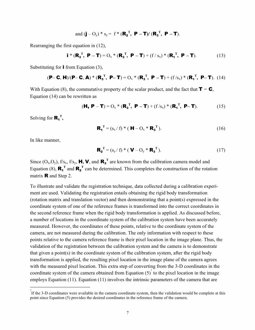
As stated before, the target shown in Figure 5 was situated in four different positions. In two of the positions, the target was upright as shown in Figure 5; in the other two positions, the target was turned upside down to provide greater variety to the data. Not including the stand, the target was approximately 2.2 meters wide and 0.955 meter high.

The four target positions and orientations are schematically shown in Figure 716

with the colors corresponding to the pixel and 3-D reconstruction colors in Figure 6. In terms of the left and right camera pixel graphs, the greater the distance of the target location from the camera (Figure 7), the smaller the size of the rectangle representing the corners of the target as is expected. However, since the 3-D reconstructed graph is the projection onto the x-y plane, the rectangles representing the target should all be the same size as shown in Figure 6. In addition, the size of the rectangles corresponds to the target size, 2.2 meters by 0.955 meter. This again demonstrates the validity of the 3-D reconstruction process developed in Sections 2 through 4. The last observation concerns the vertical location of the rectangles in the 3-D reconstruction graph. If the camera focal axis is perpendicular to the target, then the reconstructed data for the targets in the upright position should have the same y-coordinates. The same is true for the two targets in the upside down position. From Figure 6, this is not the case. In fact, for this data collection at FITG, the camera system pointed downward and the 3-D reconstructed data are in the coordinate system of the stereo system, specifically the coordinate system of the left camera. How this can cause two objects at the same height above the ground to have different vertical locations in the camera coordinate system is illustrated in Figure 8 and is related to depth perception.

Figure 7. Schematic of location (distance relative to camera reference frame) and orientation of targets.

To determine the registration between the stereo system and the LADAR system, 3-D coordinates in the LADAR coordinate system corresponding to the stereo system points are

16

Locations and distances are not accurately portrayed in the figure.

Cam

era

Position OnePosition OneUpright (~ 5 m)Upright (~ 5 m)

Position TwoPosition TwoUpright (~7.8 m)Upright (~7.8 m)

Position FourPosition FourUpside Down (~7 M)Upside Down (~7 M)

Position ThreePosition ThreeUpside Down (~8.7 m)Upside Down (~8.7 m)

19

required. In the LADAR imagery, pixel locations of the four corners are manually identified by a MATLAB program developed by NIST called “senView”

17. The pixel locations are transcribed

to a NIST program called “seoReadFromFile”18

. This program then calculates the 3-D coordi-nates of the feature in the coordinate system of the vehicle

19. Pixel locations and 3-D coordinates

obtained from the NIST LADAR system and 3-D reconstruction procedure are provided in Appendix C.

Figure 8. Effect on y-coordinate because of tilted coordinate system. With the 15 matching 3-D points (one stereo point was not visible in the LADAR data), the registration between the stereo and LADAR systems is calculated. Results are summarized next.

The model assumes that ψ = RSL * ξ + TSL,

in which the subscript SL refers to the transformation from the stereo coordinate system to the LADAR coordinate system,

ξ is a 3-D point in the coordinate system of the stereo unit (left camera coordinate system), and

17

Private communication, Tommy Chang, National Institute of Standards and Technology, Gaithersburg, MD, 2002. 18

Private communication, Tsai Hong, National Institute of Standards and Technology, Gaithersburg, MD, 2001. 19

NIST maps into the vehicle coordinate system rather than a distinct coordinate system for the LADAR. The registration of the stereo sensor to the LADAR sensor is therefore between the stereo and vehicle coordinate systems.

World Coordinate System z-axis

y-axisCamera Coordinate System

z-axis

y-axis

Two PointsSame y-coordinate

InWorld Coordinate System

i.e., same height above ground

Same Two PointsDifferent y-coordinate

InCamera Coordinate System

If TiltedStill same height above ground

20

ψ is the equivalent 3-D point in the coordinate system of the LADAR sensor (i.e., vehicle coordinate system). In this case, the units are in meters.

RSL =F

HGG

I

KJJ

0.9986656 0.0385101 - 0.0344089 - 0.0298951 0.9743899 0.2228688 0.0421103 - 0.2215428 0.9724241

and TSL = [0.1423677 -1.3482944 2.9820147]T. The projection into the x-y plane in the LADAR coordinate system of the transformation of the 15 stereo points used in determining RSL and TSL is shown in Figure 9. In the figure, the colors correspond to those in Figure 6 so that a comparison is easier. An overlay of the transformed stereo points (dashed) and the measured LADAR points (solid) projected into the x-y plane of the LADAR coordinate system is provided in Figure 10.

While the overlay of the stereo and LADAR data in Figure 10 is similar, systematic errors are evident. At best, the transformation is “in the ball park”. Errors observed in the transformation can result from systematic errors in the sensor data and from errors in the transformation function. If errors can be shown to exist in the data points used to generate the transformation function, errors in the transformed sensor data become more understandable. Toward this end, the sensor source data are evaluated for flaws via qualitative and quantitative methods.

Figure 9. Transformed stereo points to Figure 10. Overlay of transformed stereo LADAR coordinate system. (dash)and LADAR (solid) points, LADAR coordinate system.

The transformation function is calculated from a relatively small number of points “hand picked” from the stereo and LADAR images. Errors in the correspondence of these points propagate into the calculation of the transformation. Additionally, the LADAR data are known to be subject to facet error, when sub-images from different facets of the LADAR’s whirling mirrors do not align exactly in the image. This is evident in the LADAR image of Figure 5, where the straight lines

Fi 10 O l f f dFi 9 T f f i

21

comprising the sides of the target vary by a (very large) LADAR pixel. This error also finds its way into the transformation function.

To quantitatively investigate possible errors in the stereo and LADAR data, a comparison of sensor estimates of known geometric parameters of the target is performed. These parameters are embedded in the target so that ground truth is known. The parameters known with certainty are the linear dimensions of the target edges, the perpendicularity of the corners, and the planarity of the target. These can be calculated from the 3-D reconstructed stereo data and the LADAR data of the measured corner points of the target in the different poses, as follows.

The length of edges is a simple Euclidian distance between adjacent points. According to the “as-built” drawings of the registration target, the length of the horizontal edge is 2.200 meters, and the vertical edge is 0.955 meter. The length error is the difference between the “as-built” measure and the Euclidian distance between corners from the 3-D reconstructed stereo data or the measured LADAR data.

Error in the perpendicularity of the corners is the absolute value of the difference between π/2 and the angle formed between the rays defined by a corner point (e.g., UL = upper left) and its two peripheral neighbors (e.g., UR = upper right and LL = lower left) for the stereo and LADAR data. The error is given by

( ) ( ) ,*

arccos2

→→→•→

−=∠ LLULURULLLULURULπε

in which )( YYXX → represents a vector defined by points XX and YY, YYXX → its

magnitude, and • the vector scalar or dot product.

Error in planarity of the stereo and LADAR data is the distance between a plane formed by three target corner points (UL, UR, and LL) and the fourth point (LR). We compute this error by determining the unit normal vector to the plane determined by the three points UL, UR, and LL,

in which × represents vector cross product, followed by taking the dot product

Statistics from this comparison are presented in Table 1.

( ) ( )( ) ( )LLULURUL

LLULURULn→×→→×→

=

).( LRULnp →•=rε

22

Table 1. Statistics from the comparison

LADAR Stereo Length error Mean -0.0628 -0.0600 (meter) SD 0.1950 0.0883 Max 0.1434 0.0657 Angle error (abs val) Mean 4.0787 2.8515 (degrees) SD 2.4741 1.9290 Max 7.8546 7.2813 Coplanarity error View 1 0.0210 0.1334 (meter) View 2 0.0944 -0.1986 View 4 -0.0449 0.0760

Because of the much larger standard deviation, errors in the length of edges appear to be greater in the LADAR data. The target was presented to the sensors nearly perpendicularly to the axis of the sensors, so measurements of length tended to be in the “image plane” of the sensor. LADAR images are not well calibrated in this plane because of facet error (a topic beyond the scope of this report). The observed error is consistent with errors in the location of points in the image plane. The erroneous placement of points in the image plane would also account for a higher error in the corner angles calculated from the LADAR data.

The planarity error is higher in the stereo data than in the LADAR. In the images used, planarity is substantially in the direction of the sensor axes, i.e., perpendicular to the image plane. LADAR performs quite well in this axis, while stereo is subject to errors in the manual selection of matching points. Again, this error is consistent with a known and independent source of error.

Based on these observations, the data points upon which the registration is based appear to show evidence of error, which could have a deleterious impact on the transformation function and would in turn contribute to the observed error between measurements from the two sensors.

To evaluate the registration between the stereo and LADAR sensor systems, the error resulting from the transformation is evaluated. Since a surveyed location, i.e., ground truth, of the points extracted from the poses of the target is not known, the error metric selected for scrutiny is the difference between the estimates of 3-D position by the LADAR and stereo sensors. The measurements are in the LADAR sensor coordinate system and, thus, the stereo data result from the registration transformation being applied to the 3-D reconstructed stereo points. Unfortunate-ly, the points used in this error analysis are the same points used to generate the transformation. Although this situation is not desirable for drawing definitive conclusions, other points for use in the analysis are not available, and thus, the analysis provides only a “crude” indicator of the effectiveness of the method for determining the registration between the sensor systems.

Spherical rms values are shown in Figure 11 as vectors attached to the corners of the transformed stereo points from Figure 9. The magnitude of the vectors is the 3-D Euclidean distance that a stereo point needs to be moved in order to match the corresponding LADAR point. Units for the

23

vectors are the same as in the graph. The vector direction is not meaningful. The mean error is 0.2694 meter, the standard deviation 0.0848 meter, and the maximum error is 0.4204 meter. There appears to be no pattern to the errors represented by the vectors. Since the ground truth is not known, interpretation of the mean rms value is difficult. However, it may be indicative of “large” inaccuracies in the stereo and/or LADAR estimated positions and the actual positions of the features in the scene. The small rms standard deviation may be a result of the fact that the data used in generating the transformation are the same data used in the error analysis. Based on the rms mean, the authors feel that the registration results should be viewed as a “rough” approximation.

Figure 11. Error associated with the stereo-LADAR registration.

7. Summary

This report documents ARL’s methodology for performing sensor registration and 3-D reconstruction from stereo images. With a collection of procedures developed by JPL, a MATLAB program from Soder (2002), and software developed at ARL, registration between any sensor coordinate systems can be performed.

The methodology developed and presented in this report was applied to stereo and LADAR data collected at FITG. Although a registration between the two sensor systems was obtained, errors present in the data used to generate the registration appear to impact the accuracy of the

24

numerical results but not the methodology. Using additional matching stereo and LADAR points in determining the registration may provide better results.

Future data collections focusing on the development of a multi-sensor database will apply approaches described in this report and will address the issues that surfaced because of the errors in the data.

25

References

Albus, J.S., 4-D/RCS: A reference Model Architecture for Demo III, Version 1.0, NISTIR 5994, National Institute of Standards and Technology, Gaithersburg, MD, March 1997.

Gennery, D.B., Least Squares Camera Calibration Including Lens Distortion and Automatic Editing of Calibration Points, Springer Series in Information Sciences, Vol. 34, Calibration and Orientation of Cameras in Computer Vision, Eds. Gruen and Huang, Springer-Verlag, Berlin and Heidelberg, 2001.

Gennery, D.B., T. Litwin, B. Wilcox, and B. Bon. Sensing and Perception Research for Space Telerobotics at JPL, Proceedings of the IEEE International Conference on Robotics and Automation, pp. 311-317. Raleigh, NC, March 31-April 3, 1987.

Jet Propulsion Laboratory, Cahvor Camera Model Information, web site, http://robotics.jpl.nasa.gov/people/mwm/chavor.html, California Institute of Technology, Pasadena, CA, 2002.

Litwin, T., CCALDOTS, Jet Propulsion Laboratory, California Institute of Technology, Pasadena, CA, Written: 13 Mar 1991, Updated: 22 Jun 2000, Copyright (C) 1991, 1992, 1993, 1994, 1996, 1997, 1998, 1999, 2000, California Institute of Technology, all rights reserved.

Soder, M., Matlab Function to Determine Rigid Body Rotation and Translation, web site, http://isb.ri.ccf.org/software/soder.m, 2002.

Trucco, E., and A. Verri, Introductory Techniques for 3-D Computer Vision, Prentice Hall, Inc., Upper Saddle River, NJ, 1998.

Yakimovsky, Y., and R.T. Cunningham, A System for Extracting Three-Dimensional Measurements from a Stereo Pair of TV Cameras, Computer Graphics and Image Processing 7, pp 195–210, 1978.

26

INTENTIONALLY LEFT BLANK

27

Appendix A: C++ Program to Perform 3-D Reconstruction

/* This program will compute the 3D coordinates of a world point given the calibration information and a pair of conjugate points from the stereo camera pair. Command line arguments are the left and right camera calibration information: C A H V Hs Hc Vs Vc The third command line argument is the file containing the conjugate points. Each pair on the same line, left right. The final argument is the output file name. Version 1.0, May 2002, W. Oberle */ #include <iostream> #include <fstream> using namespace std; void main (int argc, char *argv[]) { float cL[3],aL[3],hL[3],vL[3],cR[3],aR[3],hR[3],vR[3]; float tL[3],tR[3],rL[3][3],rR[3][3],t[3],r[3][3],rLT[3][3], rT[3][3], A[3][3]; float hSL,hCL,vSL,vCL,hSR,hCR,vSR,vCR; float pL[3],pR[3],P[3],K[3],Q[3]; float t1; if (argc != 5) { cout << "Usage: 3d_recon left_calibration right_calibration point_file ouput_file" << endl; return; } // Read calibration information ifstream input(argv[1]); input >> cL[0] >> cL[1] >> cL[2]; input >> aL[0] >> aL[1] >> aL[2]; input >> hL[0] >> hL[1] >> hL[2]; input >> vL[0] >> vL[1] >> vL[2]; input >> hSL; input >> hCL; input >> vSL; input >> vCL;

28

input.close(); ifstream input1(argv[2]); input1 >> cR[0] >> cR[1] >> cR[2]; input1 >> aR[0] >> aR[1] >> aR[2]; input1 >> hR[0] >> hR[1] >> hR[2]; input1 >> vR[0] >> vR[1] >> vR[2]; input1 >> hSR; input1 >> hCR; input1 >> vSR; input1 >> vCR; input1.close(); // Create rigid body rotation and translation from calibration to // left/right camera for (int i = 0; i < 3; i++) { tL[i] = cL[i]*25.4; // Convert to mm from inches tR[i] = cR[i]*25.4; rL[2][i] = aL[i]; rR[2][i] = aR[i]; rL[0][i] = (hL[i]-hCL*rL[2][i])/hSL; rR[0][i] = (hR[i]-hCR*rR[2][i])/hSR; rL[1][i] = (vL[i]-vCL*rL[2][i])/vSL; rR[1][i] = (vR[i]-vCR*rR[2][i])/vSR; } // Create rigid body rotation and translation between left and right // camera for (i = 0; i < 3; i++) { t[i]=0; for (int j = 0; j < 3; j++) { rLT[i][j] = rL[j][i]; r[i][j] = 0; t[i] += rL[i][j]*(tR[j]-tL[j]); } } for (i = 0; i < 3; i++) for (int j = 0; j < 3; j++){ for (int k = 0; k < 3; k++){ r[i][j] += rR[i][k]*rLT[k][j]; } } for (i = 0; i < 3; i++) for (int j = 0; j < 3; j++) rT[i][j] = r[j][i]; // Now the points are read until an EOF is reached. ifstream input2(argv[3], ios::in | ios::binary); ofstream output(argv[4]); output << "Left Image In Pixels:\nRight Image In Pixels:\n3D Point (mm):\n3D Point (inches)\n\n";

29

int kount = 1; while (input2 >> pL[0] >> pL[1] >> pR[0] >> pR[1]) { //input2 >> pL[0] >> pL[1] >> pR[0] >> pR[1]; output << "Point Number: " << kount++ << endl; output << pL[0] << " " << pL[1] << endl; output << pR[0] << " " << pR[1] << endl; A[0][0] = pL[0] = (pL[0]-hCL)/hSL; A[1][0] = pL[1] = (pL[1]-vCL)/vSL; A[2][0] = pL[2] = 1; pR[0] = (pR[0]-hCR)/hSR; pR[1] = (pR[1]-vCR)/vSR; pR[2] = 1; for (i = 0; i < 3; i++) { K[i]=0; P[i] = t[i]; for (int j = 0; j < 3; j++) { K[i] += rT[i][j]*pR[j]; } A[i][1] = -K[i]; } A[0][2] = pL[1]*K[2]-K[1]*pL[2]; A[1][2] = -(pL[0]*K[2]-K[0]*pL[2]); A[2][2] = pL[0]*K[1]-K[0]*pL[1]; t1 = P[0]; P[0] = P[2]; P[2] = t1; for (i = 0; i < 3; i++) { t1 = A[0][i]; A[0][i] = A[2][i]; A[2][i] = t1; } // Gauss Jordan Elimination -- Col 1 t1 = -A[1][0]; A[1][1] += t1*A[0][1]; P[1] += t1*P[0]; A[1][2] += t1*A[0][2]; t1 = -A[2][0]; A[2][1] += t1*A[0][1]; A[2][2] += t1*A[0][2]; P[2] += t1*P[0]; // Now Col 2 t1 = A[1][1]; A[1][2] /= t1; P[1] /= t1; t1 = -A[0][1]; A[0][2] += t1*A[1][2]; P[0] += t1*P[1];

30

t1 = -A[2][1]; A[2][2] += t1*A[1][2]; P[2] += t1*P[1]; // Now Col 3 t1 = A[2][2]; P[2] /= t1; P[0] += -A[0][2]*P[2]; P[1] += -A[1][2]*P[2]; for (i = 0; i < 3; i++) { Q[i] = .5* (P[0]*pL[i]+t[i]+P[1]*K[i]); } output << Q[0] << " " << Q[1] << " " << Q[2] << endl; output << Q[0]/25.4 << " " << Q[1]/25.4 << " " << Q[2]/25.4 << endl; output << "**********\n\n"; } input2.close(); output.close(); return; }

31

Appendix B: Three-Dimensional Reconstruction for Stereo Data Used in Stereo-LADAR Registration, Based on Results of Program of Appendix A

regCoord Gary Haas 9/5/2002 //Raw image data - hand-picked points at 4 corners of the registration target // conventional image coordinates, e.g. origin is at top left of image //1a from stereo seq #4 (nist numbering system) -- //left cam right camera //col row col row 175 40 130 38 //1a Top Left 521 38 465 31 //TR 523 188 468 176 //BR 180 196 138 187 //BL //2a from seq #5 219 77 192 73 //2a Top Left 220 180 194 171 //Bottom Left 450 179 416 169 //Bottom Right 451 79 415 71 //Top Right //3a from seq #6 430 184 400 173 //3a 430 275 401 262 630 273 595 257 631 184 595 172 //4a from seq #7 41 198 18 190 //4a 44 317 23 305 307 311 273 298 307 195 272 186 Image in coordinate system of left camera: x parallel to horizontal scan line (right positive from behind camera), y down (in image) z perpendicular to image plane, (lens points in positive direction) 3D reconstructed from epipolar geometry based on hand-picked corner points using the July 2002 stereo calibration. Stereo reconstruction based on calibration of July 2002 Left Image In Pixels: Right Image In Pixels:

32

3D Point (m): 3D Point (inches) Point Number: 1 175 40 130 38 -1.03703 -1.16447 5.02968 -40.8278 -45.8453 198.019 ********** Point Number: 2 521 38 465 31 0.974732 -1.20268 5.09194 38.3753 -47.3497 200.47 ********** Point Number: 3 523 188 468 176 1.0187 -0.33829 5.25797 40.1063 -13.3185 207.007 ********** Point Number: 4 180 196 138 187 -1.07263 -0.283746 5.34585 -42.2294 -11.1711 210.467 ********** Point Number: 5 219 77 192 73 -1.18727 -1.44458 7.63003 -46.7428 -56.8733 300.395 ********** Point Number: 6 220 180 194 171 -1.22415 -0.568194 7.91569 -48.1949 -22.3698 311.641 ********** Point Number: 7 450 179 416 169 0.872781 -0.584932 7.9491 34.3615 -23.0288 312.957 ********** Point Number: 8 451 79 415 71 0.828497 -1.41224 7.46903 32.618 -55.6001 294.056

33

********** Point Number: 9 430 184 400 173 0.761024 -0.599191 8.77007 29.9616 -23.5902 345.278 ********** Point Number: 10 430 275 401 262 0.792545 0.336891 9.12961 31.2026 13.2634 359.433 ********** Point Number: 11 630 273 595 257 2.83513 0.290651 8.94699 111.619 11.443 352.244 ********** Point Number: 12 631 184 595 172 2.71647 -0.589137 8.54325 106.948 -23.1944 336.349 ********** Point Number: 13 41 198 18 190 -2.48799 -0.345475 6.90508 -97.9522 -13.6014 271.854 ********** Point Number: 14 44 317 23 305 -2.56781 0.629459 7.19639 -101.095 24.7818 283.323 ********** Point Number: 15 307 311 273 298 -0.385101 0.559421 7.05714 -15.1614 22.0245 277.84 ********** Point Number: 16 307 195 272 186 -0.374484 -0.372331 6.8616 -14.7435 -14.6587 270.142

34

INTENTIONALLY LEFT BLANK

35

Appendix C: Results of LADAR 3-D Reconstruction With NIST Procedure Data Used in Stereo-LADAR Registration

LADARRegPoints Gary Haas 9/5/2002 Hand-picked points from LADAR images of the registration target used during the multispectral data collection of UGV autonomous mobility sensor data, FITG May 22 2002. Corners of the target were picked in the display of the senView program, pixel coordinates were transcribed to program seoReadFromFile which generated 3D coordinates. senView seoReadFromFile fw_04 r c d r c x y z UL 2 49 5.7 31 48 -1.332659 -1.329297 8.137999 BL 17 51 5.625 16 50 -1.231865 -0.278566 8.042555 BR 16 97 17 96 0.747331 -0.315288 8.261327 UR 1 98 32 97 0.801027 -1.231137 8.381081 fw_05 r c d r c x y z UL 3 60 8.175 30 59 -1.329650 -1.253802 10.786284 BL 14 61 8.175 19 60 -1.258575 -0.206635 10.682516 BR 14 94 8.175 19 93 0.564756 -0.172824 10.736829 UR 2 94 8.25 31 93 0.564188 -1.183124 10.934067 fw_06 r c d r c x y z UL 14 89 9.075 19 88 0.893189 -0.060707 11.777825 BL 25 89 9.075 ??? 8 88 0.890459 0.933510 11.543126 BR can't identify the corner in the data UR 14 118 9.375 19 117 2.627990 -0.080651 11.883673 fw_07 r c d r c x y z UL 16 38 7.5 17 37 -2.715522 -0.153236 9.639578 BL 27 39 7.575 6 38 -2.566245 0.842575 9.345659 BR 29 70 7.125 4 69 -0.436348 0.914655 9.623433 UR 16 71 7.2 17 70 -0.387880 -0.111421 9.907318 Note: Due to differences in the image coordinate system between the two NIST programs, the row and column differ as follows. rsRFF = 33 - rsV csRFF = csV - 1 [This has been corrected in a newer version of seoReadFromFile]. The d value reported by senView is a raw distance (apparently from the sensor), while the 3D coordinates reported by seoReadFromFile are in the coordinate system of the HMMWV on which the equipment is mounted.

36

INTENTIONALLY LEFT BLANK

REPORT DOCUMENTATION PAGE

1. AGENCY USE ONLY (Leave blank)

4. TITLE AND SUBTITLE

7. PERFORMING ORGANIZATION NAME(S) AND ADDRESS(ES)

9. SPONSORING/MONITORING AGENCY NAME(S) AND ADDRESS(ES)

11. SUPPLEMENTARY NOTES

12a. DISTRIBUTION/AVAILABILITY STATEMENT 12b. DISTRIBUTION CODE

14. SUBJECT TERMS

13. ABSTRACT (Maximum 200 words)

5. FUNDING NUMBERS

20. LIMITATION OF ABSTRACT

NSN 7540-01-280-5500

Form ApprovedOMB No. 0704-0188

Public reporting burden for this collection of information is estimated to average 1 hour per response, including the time for reviewing instructions, searching existing data sources, gathering and maintaining the data needed, and completing and reviewing the collection of information. Send comments regarding this burden estimate or any other aspect of this collection of information, including suggestions for reducing this burden, to Washington Headquarters Services, Directorate for Information Operations and Reports, 1215 Jefferson Davis Highway, Suite 1204, Arlington, VA 22202-4302, and to the Office of Management and Budget, Paperwork Reduction Project (0704-0188), Washington, DC 20503.

2. REPORT DATE 3. REPORT TYPE AND DATES COVERED

6. AUTHOR(S)

8. PERFORMING ORGANIZATION REPORT NUMBER

10. SPONSORING/MONITORING AGENCY REPORT NUMBER

15. NUMBER OF PAGES

16. PRICE CODE

17. SECURITY CLASSIFICATION OF REPORT

18. SECURITY CLASSIFICATION OF THIS PAGE

19. SECURITY CLASSIFICATION OF ABSTRACT

Standard Form 298 (Rev. 2-89)Prescribed by ANSI Std. Z39-18298-102

ARL-TR-2878

December 2002

Unclassified Unclassified Unclassified

Final

PR: 622618AH03

U.S. Army Research LaboratoryWeapons & Materials Research Directorate Aberdeen Proving Ground, MD 21005-5066

37

Oberle, W.F.; Haas, G.A. (both of ARL)

45

Three-Dimensional Stereo Reconstruction and Sensor Registration with Application to the Development of a Multi-Sensor Database

camera calibration stereoscopic video sensor registration three-dimensional reconstruction

Approved for public release; distribution is unlimited.

This report discusses efforts undertaken at the U.S. Army Research Laboratory (ARL), which support research in robotic perception. The efforts include collaborative work with the National Institute of Standards and Technology to develop a multi-sensor (laser radar [LADAR], navigation and stereoscopic video [stereo]) database with ground truth for use by the robotics research community. ARL’s efforts are focused on stereo. The report documents procedures for determining the transformations between the cameras of the stereo system and the transformations between the camera system and other sensor, vehicle, and world coordinate systems. Results indicate that the measured stereo and ladar data are susceptible to large errors that affect the accuracy of the calculated transformations.