three essays on big data consumer analytics in e-commerce
TRANSCRIPT

University of Pennsylvania University of Pennsylvania
ScholarlyCommons ScholarlyCommons
Publicly Accessible Penn Dissertations
2015
Three Essays on Big Data Consumer Analytics in E-Commerce Three Essays on Big Data Consumer Analytics in E-Commerce
Dokyun Lee University of Pennsylvania, [email protected]
Follow this and additional works at: https://repository.upenn.edu/edissertations
Part of the Advertising and Promotion Management Commons, Databases and Information Systems
Commons, and the Marketing Commons
Recommended Citation Recommended Citation Lee, Dokyun, "Three Essays on Big Data Consumer Analytics in E-Commerce" (2015). Publicly Accessible Penn Dissertations. 1830. https://repository.upenn.edu/edissertations/1830
This paper is posted at ScholarlyCommons. https://repository.upenn.edu/edissertations/1830 For more information, please contact [email protected].

Three Essays on Big Data Consumer Analytics in E-Commerce Three Essays on Big Data Consumer Analytics in E-Commerce
Abstract Abstract Consumers are increasingly spending more time and money online. Business
to consumer e-commerce is growing on average of 20 percent each year and
has reached 1.5 trillion dollars globally in 2014. Given the scale and growth
of consumer online purchase and usage data, firms' ability to understand
and utilize this data is becoming an essential competitive strategy.
But, large-scale data analytics in e-commerce is still at its nascent stage and there
is much to be learned in all aspects of e-commerce. Successful analytics on big data often require a combination of both data mining and econometrics: data mining to reduce or structure
(from unstructured data such as text, photo, and video) large-scale data
and econometric analyses to truly understand and assign causality to interesting
patterns. In my dissertation, I study how firms can better utilize big data
analytics and specific applications of machine learning techniques for improved
e-commerce using theory-driven econometrical and experimental studies. I
show that e-commerce managers can now formulate data-driven strategies for
many aspect of business including cross-selling via recommenders on sales
sites to increasing brand awareness and leads via social media content-engineered-marketing.
These results are readily actionable with far-reaching economical consequences.
Degree Type Degree Type Dissertation
Degree Name Degree Name Doctor of Philosophy (PhD)
Graduate Group Graduate Group Operations & Information Management
First Advisor First Advisor Kartik Hosanagar
Keywords Keywords big data, data mining, e-commerce, managerial implications, recommender system, social media marketing

Subject Categories Subject Categories Advertising and Promotion Management | Databases and Information Systems | Marketing
This dissertation is available at ScholarlyCommons: https://repository.upenn.edu/edissertations/1830

THREE ESSAYS ON BIG DATA CONSUMER ANALYTICS IN E-COMMERCE
Dokyun Lee
A DISSERTATION
in
Operation and Information Management
For the Graduate Group in Managerial Science and Applied Economics
Presented to the Faculties of the University of Pennsylvania
in
Partial Fulfillment of the Requirements for the
Degree of Doctor of Philosophy
2015
Supervisor of Dissertation
Kartik Hosanagar, Professor of OPIM
Graduate Group Chairperson
Eric Bradlow, Professor of Marketing,Statistics, and Education
Dissertation Committee
Kartik Hosanagar, Professor of Operations and Information ManagementLorin M. Hitt, Class of 1942 Professor of Operations and Information ManagementHarikesh S. Nair, Professor of Marketing, Stanford Graduate School of Business

THREE ESSAYS ON BIG DATA CONSUMER ANALYTICS IN E-COMMERCE
© COPYRIGHT
2015
Dokyun Lee
This work is licensed under the
Creative Commons Attribution
NonCommercial-ShareAlike 3.0
License
To view a copy of this license, visit
http://creativecommons.org/licenses/by-nc-sa/3.0/

Dedicated to my parents, Hongme and Sangwook,
and my sister, Soyeon.
iii

ACKNOWLEDGEMENT
The five years I spent here has been the best time of my life thus far. I am grateful for the
best advisors and friendly colleagues who have helped and stimulated me throughout.
I would like to first thank my advisor, Kartik Hosanagar, who goes above and beyond for
his students with a style and grace. I would like to thank Lorin Hitt and Harikesh Nair for
being in my committee and for giving me valuable advices and feedbacks on both research
and career. I am blessed to have world-leading researchers and educators as my mentors,
who excel in advising and guiding as much as they do in researching and teaching. I learned
many things beyond researching from them and I hope to learn even more in the decades
to come. I am grateful for insightful discussions and general supports from Vibhanshu
Abhishek, Christophe Van den Bulte, Raghuram Iyengar, David Bell, Jonah Berger, Dylan
Small, Dean Foster, Paul Shaman, Lynn Wu, Xuanming Xu, Noah Gans, Eric Clemons,
Jing Peng, Fujie Jin, Eric Bradlow, Karl Ulrich, Jeff Cai, and Arun Gopalakrishnan.
I would like to thank the Baker Retailing Center, the William And Phyllis Mack Institute
for Innovation Management, Fishman-Davidson Center for Service and Operations Man-
agement, and Wharton Risk Management and Decision Processes Center for their generous
and instrumental financial support. I am grateful to Sargent Shriver, Andrea Nurse, Kim
Watford, Patricia James, Tara Mullins for all the administrative help and Stan Liu and
Jamie Walter for IT support.
Lastly, I would like to thank my parents for providing me with the best opportunities
possible for following any goals and dreams I have. They have been my role models all my
life and I am forever grateful for their steadfast support and unconditional sacrifice. Finally,
most opportunities I was given was possible largely thanks to my lovely sister.
iv

ABSTRACT
THREE ESSAYS ON BIG DATA CONSUMER ANALYTICS IN E-COMMERCE
Dokyun Lee
Kartik Hosanagar
Consumers are increasingly spending more time and money online. Business to consumer
e-commerce is growing on average of 20 percent each year and has reached 1.5 trillion
dollars globally in 2014. Given the scale and growth of consumer online purchase and usage
data, firms’ ability to understand and utilize this data is becoming an essential competitive
strategy. But, large-scale data analytics in e-commerce is still at its nascent stage and
there is much to be learned in all aspects of e-commerce. Successful analytics on big data
often require a combination of both data mining and econometrics: data mining to reduce
or structure (from unstructured data such as text, photo, and video) large-scale data and
econometric analyses to truly understand and assign causality to interesting patterns. In my
dissertation, I study how firms can better utilize big data analytics and specific applications
of machine learning techniques for improved e-commerce using theory-driven econometrical
and experimental studies. I show that e-commerce managers can now formulate data-driven
strategies for many aspect of business including cross-selling via recommenders on sales sites
to increasing brand awareness and leads via social media content-engineered-marketing.
These results are readily actionable with far-reaching economical consequences.
v

TABLE OF CONTENTS
ACKNOWLEDGEMENT . . . . . . . . . . . . . . . . . . . . . . . . . . . . . . . . . iv
ABSTRACT . . . . . . . . . . . . . . . . . . . . . . . . . . . . . . . . . . . . . . . . v
LIST OF TABLES . . . . . . . . . . . . . . . . . . . . . . . . . . . . . . . . . . . . . ix
LIST OF ILLUSTRATIONS . . . . . . . . . . . . . . . . . . . . . . . . . . . . . . . xi
CHAPTER 1 : Introduction . . . . . . . . . . . . . . . . . . . . . . . . . . . . . . . 1
CHAPTER 2 : The Effect of Social Media Marketing Content on Consumer Engage-
ment: Evidence from Facebook . . . . . . . . . . . . . . . . . . . . 5
2.1 Introduction . . . . . . . . . . . . . . . . . . . . . . . . . . . . . . . . . . . . 5
2.2 Data . . . . . . . . . . . . . . . . . . . . . . . . . . . . . . . . . . . . . . . . 12
2.3 Empirical Strategy . . . . . . . . . . . . . . . . . . . . . . . . . . . . . . . . 29
2.4 Results . . . . . . . . . . . . . . . . . . . . . . . . . . . . . . . . . . . . . . . 37
2.5 Discussion and Managerial Implications . . . . . . . . . . . . . . . . . . . . 50
2.6 Conclusions . . . . . . . . . . . . . . . . . . . . . . . . . . . . . . . . . . . . 54
CHAPTER 3 : People Who Liked This Study Also Liked: The Impact of Recom-
mender Systems on Sales Volume and Diversity . . . . . . . . . . . 56
3.1 Introduction . . . . . . . . . . . . . . . . . . . . . . . . . . . . . . . . . . . . 56
3.2 Prior Work . . . . . . . . . . . . . . . . . . . . . . . . . . . . . . . . . . . . 59
3.3 Problem Formulation . . . . . . . . . . . . . . . . . . . . . . . . . . . . . . . 64
3.4 Data . . . . . . . . . . . . . . . . . . . . . . . . . . . . . . . . . . . . . . . . 69
3.5 Results . . . . . . . . . . . . . . . . . . . . . . . . . . . . . . . . . . . . . . . 72
3.6 Discussion and Conclusion . . . . . . . . . . . . . . . . . . . . . . . . . . . . 85
vi

CHAPTER 4 : When do Recommender Systems Work the Best? The Moderating
Effects of Product Attributes and Consumer Reviews on Recom-
mender Performance . . . . . . . . . . . . . . . . . . . . . . . . . . 88
4.1 Introduction . . . . . . . . . . . . . . . . . . . . . . . . . . . . . . . . . . . . 88
4.2 Data . . . . . . . . . . . . . . . . . . . . . . . . . . . . . . . . . . . . . . . . 91
4.3 Product Attributes & Hypotheses . . . . . . . . . . . . . . . . . . . . . . . . 95
4.4 Model & Results . . . . . . . . . . . . . . . . . . . . . . . . . . . . . . . . . 106
4.5 Conclusion and Discussion . . . . . . . . . . . . . . . . . . . . . . . . . . . . 111
APPENDIX . . . . . . . . . . . . . . . . . . . . . . . . . . . . . . . . . . . . . . . . . 123
BIBLIOGRAPHY . . . . . . . . . . . . . . . . . . . . . . . . . . . . . . . . . . . . . 125
vii

LIST OF TABLES
TABLE 1 : Variable Descriptions and Summary for Content-coded Data . . . . 18
TABLE 2 : Examples of Messages and Their Content Tags . . . . . . . . . . . 19
TABLE 3 : Performance of Text Mining Algorithm on 5000 Messages Using 10-
fold Cross-validation . . . . . . . . . . . . . . . . . . . . . . . . . . 28
TABLE 4 : User-level Setup Notation. . . . . . . . . . . . . . . . . . . . . . . . 31
TABLE 5 : EdgeRank Model Estimates . . . . . . . . . . . . . . . . . . . . . . 39
TABLE 6 : Persuasive vs Informative . . . . . . . . . . . . . . . . . . . . . . . 41
TABLE 7 : Aggregate Logistic Regression Results For Comments and Likes . . 45
TABLE 8 : Predicted versus Actual Engagement Ranking for Three Illustrative
messages . . . . . . . . . . . . . . . . . . . . . . . . . . . . . . . . . 53
TABLE 9 : Literature on Impact of Recommender Systems and Claims . . . . 63
TABLE 10 : Movie Genres Viewed and Purchased . . . . . . . . . . . . . . . . . 71
TABLE 11 : Data Summary Statistics . . . . . . . . . . . . . . . . . . . . . . . . 73
TABLE 12 : Individual Item Views Comparison . . . . . . . . . . . . . . . . . . 76
TABLE 13 : Individual Item Purchases Comparison . . . . . . . . . . . . . . . . 76
TABLE 14 : Individual Wallet-Size Comparison . . . . . . . . . . . . . . . . . . 77
TABLE 15 : Aggregate View Diversity . . . . . . . . . . . . . . . . . . . . . . . 78
TABLE 16 : Aggregate Sales Diversity . . . . . . . . . . . . . . . . . . . . . . . 78
TABLE 17 : Individual View Diversity . . . . . . . . . . . . . . . . . . . . . . . 79
TABLE 18 : Individual Purchase Diversity . . . . . . . . . . . . . . . . . . . . . 80
TABLE 19 : Hypotheses Tested . . . . . . . . . . . . . . . . . . . . . . . . . . . 82
TABLE 20 : Permutation Test Results for Co-purchase Network Comparisons . 83
TABLE 21 : Hypotheses under Robustness Checks . . . . . . . . . . . . . . . . . 86
TABLE 22 : Product Categories Occurring In the Dataset . . . . . . . . . . . . 93
viii

TABLE 23 : Variable Descriptions and Summary for Content-coded Data. . . . 94
TABLE 24 : Utilitarian VS. Hedonic Product Cluster Means . . . . . . . . . . . 99
TABLE 25 : Search VS. Experience Product Cluster Means . . . . . . . . . . . . 103
TABLE 26 : Logistic Regression Results Table . . . . . . . . . . . . . . . . . . . 107
TABLE 27 : Multiple Specifications for Review Related Variables . . . . . . . . 110
TABLE 28 : Hypotheses and Results . . . . . . . . . . . . . . . . . . . . . . . . 110
TABLE 29 : Other Takeaways . . . . . . . . . . . . . . . . . . . . . . . . . . . . 111
TABLE 30 : A Few Examples of Message Attributes Used in Natural Language
Processing Algorithm . . . . . . . . . . . . . . . . . . . . . . . . . . 120
TABLE 31 : Performance of Text Mining Algorithm on 5000 Messages Using 10-
fold Cross-validation . . . . . . . . . . . . . . . . . . . . . . . . . . 121
TABLE 32 : Survey Instrument . . . . . . . . . . . . . . . . . . . . . . . . . . . 124
ix

LIST OF ILLUSTRATIONS
FIGURE 1 : (Left) Example of a firm’s Facebook Page (Walmart). (Right) Ex-
ample of a firm’s message and subsequent user engagement with
that message (Tennis Warehouse). Example is not necessarily from
our data. . . . . . . . . . . . . . . . . . . . . . . . . . . . . . . . . 13
FIGURE 2 : Co-occurrence of Attribute Characteristics Across messages . . . . 20
FIGURE 3 : Bubble Chart of Broader Industry Category vs Message Content . 21
FIGURE 4 : Box Plots of Log(engagement+1) vs Time since message Release . 22
FIGURE 5 : Average Likes and Comments by Message Type . . . . . . . . . . 23
FIGURE 6 : Average Likes and Comments by Message Type by Industry . . . 23
FIGURE 7 : Average Likes and Comments by Message Content . . . . . . . . 24
FIGURE 8 : Cronbach’s Alphas for 5,000 Messages . . . . . . . . . . . . . . . . 25
FIGURE 9 : Impression-Engagement Funnel . . . . . . . . . . . . . . . . . . . 31
FIGURE 10 : Page-level Fixed effect Estimates from Generalized Additive Model
Across 14 Demographic Bins . . . . . . . . . . . . . . . . . . . . . 40
FIGURE 11 : Time Since message Release (τ) Coefficients Box plot Across De-
mographics . . . . . . . . . . . . . . . . . . . . . . . . . . . . . . . 40
FIGURE 12 : Message Characteristic Coefficients for Comments and Likes . . . 46
FIGURE 13 : Logistic Regression by Industry . . . . . . . . . . . . . . . . . . . 47
FIGURE 14 : Proportion of Content Posted Split into Hour-bin . . . . . . . . . 49
FIGURE 15 : Message Characteristic Coefficients for Shares and Click-throughs 52
FIGURE 16 : Lorenz Curve . . . . . . . . . . . . . . . . . . . . . . . . . . . . . 65
FIGURE 17 : Recommender Example . . . . . . . . . . . . . . . . . . . . . . . . 70
FIGURE 18 : Average Individual Statistics . . . . . . . . . . . . . . . . . . . . . 74
FIGURE 19 : Lorenz Curves for Movie Genres Purchased . . . . . . . . . . . . . 75
x

FIGURE 20 : Co-Purchase Network Graphs of Genre Purchases under Control
and Purchase-Based Collaborative Filtering. . . . . . . . . . . . . 83
FIGURE 21 : Genre Purchase Share Comparison on Purchase-based CF vs. Control 84
FIGURE 22 : Recommendation Panel . . . . . . . . . . . . . . . . . . . . . . . . 93
FIGURE 23 : Survey Form Used in Amazon Mechanical Turk . . . . . . . . . . 113
FIGURE 24 : Diagram of NLP Training and Tagging Procedure . . . . . . . . . 119
xi

CHAPTER 1 : Introduction
Consumers are increasingly spending more time and money online. A 2013 study (eMar-
keter, 2013b) reports that for the first time, the average adult in the US will spend more
time online than watching TV at just above five hours per day. The spread of mobile devices
like smartphones and tablet PCs are also fueling this dramatic increase in consumer online
activities. Consequently, e-commerce is growing faster than ever. Business to consumer
e-commerce is growing on average of 20% each year and has reached $1.5 trillion globally
in 2014 (eMarketer, 2014).
This growth in online activity has given arise to a new phenomenon called “big data”. “Big
data” is a catch-phrase used to describe massive data recorded online (e.g., e-commerce,
search engine) and offline by a myriad of sensors (e.g., surveillance, traffic monitor). The
term is used to describe four different aspects of challenges arising from exploding data: 1)
Volume, which refers to the sheer amount of volume recorded1; 2) Variety, arising from un-
structured data like text and photos that come from numerous sources such as social media
sites; 3) Velocity, which refers to the speed at which data gets recorded; and 4) Veracity,
which refers to the uncertainty and missing data. The “big data” phenomenon has created
problems and challenges to virtually everyone including marketers, business managers, aca-
demics, and policy makers: How can big data be utilized for improved marketing, business
managing, and policy making?
Given the scale and growth of consumer online purchase and usage data, firms’ ability to
understand and utilize this big data is becoming an essential competitive strategy. Several
academic and industry reports (Kiron et al., 2011; Rogers and Sexton, 2012; Monetate,
2014a,b) show that while 63% of organizations see big data analytics as a competitive
advantage, 80% of marketers say they don’t know how to translate data into action and
that 95% of data within organizations remain unused. Even more perplexing, one survey
1In 2010, Eric Schmidt, the CEO of Google, famously mentioned that every two days, the world createsas much information as it did from the dawn of civilization up until 2003, or five exabytes of data (1 exabyte= 1 billion gigabytes).
1

(Allen et al., 2005) shows that while 80% of CEOs believe they deliver superior customer
experience, only 8% of customers agree. Big data analytics in e-commerce is still at its
nascent stage and there is much to be learned in all aspects of e-commerce. Particularly
lacking is the area of social media marketing (specifically, content engineering for better
engagement) and the impact of recommender systems, in which there are little to no large-
scale level analyses or much disagreement on what strategies actually work.
Big data analytics is challenging because successful analytics on big data often require a
combination of both data mining and econometrics: Data mining to reduce or structure
(from unstructured data such as text, photo, and video) large-scale data and econometric
analyses to truly understand and assign causality to interesting patterns. In my disserta-
tion, I study how firms can better utilize big data analytics and specific applications of
machine learning techniques for improved e-commerce using theory-driven econometrical
and experimental studies. Specifically, in the first essay, I investigate how firms can actively
content engineer their social media page postings (e.g., Facebook Pages and Twitter) to
better engage connected consumers. In the second essay, I investigate how different recom-
mender algorithms on e-commerce sites (e.g., Amazon.com’s “Consumers who purchased
this also purchased”) influence sales volume and diversity. In the third essay, I plan to study
how product attributes and reviews moderate the performance of recommender systems.
Based on completed results, it can be observed that big data analytics that combine data
mining and econometrical studies can provide readily actionable strategies to improve many
aspects of e-commerce with far-reaching economical consequences. A detailed description
of three essays is given below.
Essay 1- The Effect of Social Media Marketing Content on Consumer Engage-
ment: Evidence from Facebook We investigate the effect of social media content on
customer engagement using a large-scale field study on Facebook. We content-code more
than 100,000 unique messages across 800 companies engaging with users on Facebook using
a combination of Amazon Mechanical Turk and state-of-the-art Natural Language Process-
2

ing algorithms. We use this large-scale database of advertising attributes to test the effect
of ad content on subsequent user engagement defined as Likes and comments − with the
messages. We develop methods to account for potential selection biases that arise from
Facebook’s filtering algorithm, EdgeRank, that assigns posts non-randomly to users. We
find that inclusion of persuasive content − like emotional and philanthropic content − in-
creases engagement with a message. We find that informative content − like mentions of
prices, availability and product features − reduce engagement when included in messages
in isolation, but increase engagement when provided in combination with persuasive at-
tributes. Persuasive content thus seems to be the key to effective engagement. Our results
inform advertising design in social media, and the methodology we develop to content-code
large-scale textual data provides a framework for future studies on unstructured natural
language data such as advertising content or product reviews.
Essay 2- “People Who Liked This Study Also Liked”: An Empirical Investi-
gation of the Impact of Recommender Systems on Sales Volume and Diversity
We investigate the impact of collaborative filtering recommender algorithms (e.g., Ama-
zon.com’s “Customers who bought this item also bought”), commonly used in e-commerce,
on sales volume and diversity. We use data from a randomized field experiment on movie
sales run by a top retailer in North America. For sales volume, we show that different al-
gorithms have differential impacts. Purchase-based collaborative filtering (“Customers who
bought this item also bought”) causes a 25% lift in views and a 35% lift in the number of
items purchased over the control group (no recommender). In contrast, View-based collab-
orative filtering (“Customers who viewed this item also viewed”) shows only a 3% lift in
views and a 9% lift in the number of items purchased, albeit not statistically significant. For
sales diversity, we find that collaborative filtering algorithms cause individuals to discover
and purchase a greater variety of products but push users to the same set of titles, leading
to concentration bias at the aggregate level. We show that this differential impact on in-
dividual versus aggregate diversity is caused by users exploring into only a few ’pathway’
popular genres. That is, the recommenders were more effective in aiding discovery for a
3

few popular genres rather than uniformly aiding discovery in all genres. For managers, our
results inform personalization and recommender strategy in e-commerce. From an academic
standpoint, we provide the first empirical evidence from a randomized field experiment to
help reconcile opposing views on the impact of recommenders on sales diversity.
Essay 3- When do Recommender Systems Work the Best? The Moderating
Effects of Product Attributes and Consumer Reviews on Recommender Perfor-
mance We investigate the moderating effect of product attributes and consumer reviews
on the efficacy of a collaborative filtering recommender system on an e-commerce site. We
run a randomized field experiment on a top North American retailer’s website with 184,375
users split into a recommender-treated group and a control group with 37,215 unique prod-
ucts in the dataset. By augmenting the dataset with Amazon Mechanical Turk tagged
product attributes and consumer reviews from the website, we study their moderating in-
fluence on recommenders in generating conversion.
We first confirm that the use of recommenders increases the baseline conversion rate by
5.9%. We find that recommenders act as substitutes for high average review ratings and
review volumes with the effect of using recommenders increasing the conversion as much
as about two additional average star ratings. Additionally, we find that positive impact
on conversion from recommenders are greater for hedonic products compared to utilitarian
products while search-experience quality did not have any impact. Lastly, we find that
the higher the price, the lower the positive impact of recommenders, while providing more
product descriptions increased the recommender effectiveness.
For managers, we 1) identify the products with which to use recommenders and 2) show
how other product information sources on e-commerce sites interact with recommenders.
From an academic standpoint, we provide insight into the underlying mechanism behind
how recommenders cause consumers to purchase.
4

CHAPTER 2 : The Effect of Social Media Marketing Content on Consumer
Engagement: Evidence from Facebook
2.1. Introduction
Social networks are increasingly taking up a greater share of consumers’ time spent online.
As a result, social media — which includes advertising on social networks and/or marketing
communication with social characteristics — is becoming a larger component of firms’ mar-
keting budgets. Surveying 4, 943 marketing decision makers at U.S. companies, the 2013
Chief Marketing Officer survey (www.cmosurvey.org) reports that expected spending on
social media marketing will grow from 8.4%s of firms’ total marketing budgets in 2013 to
about 22% in the next five years. As firms increase their social media activity, the role
of content engineering has become increasingly important. Content engineering seeks to
develop content that better engages targeted users and drives the desired goals of the mar-
keter from the campaigns they implement. This raises the question: what content works
best? The most important body of academic work on this topic is the applied psychology
and consumer behavior literature which has discussed ways in which the content of market-
ing communication engages consumers and captures attention. However, most of this work
has tested and refined theories about content primarily in laboratory settings. Surprisingly,
relatively little has been explored systematically about the empirical consequences of adver-
tising and promotional content in real-world, field settings outside the laboratory. Despite
its obvious relevance to practice, Marketing and advertising content is also relatively under
emphasized in economic theory. The canonical economic model of advertising as a signal
(c.f. Nelson (1970); Kihlstrom and Riordan (1984); Milgrom and Roberts (1986)) does not
postulate any direct role for ad content because advertising intensity conveys all relevant
information about product quality in equilibrium to market participants. Models of infor-
mative advertising (c.f. Butters (1977); Grossman and Shapiro (1984)) allow for advertising
to inform agents only about price and product existence — yet, casual observation and
several studies in lab settings (c.f. Armstrong (2010); Berger (2012)) suggest that adver-
5

tisements contain much more information and content beyond prices. In this paper, we
explore the role of content in driving consumer engagement in social media in a large-scale
field setting. We document the kinds of content used by firms in practice. We show that
a variety of emotional, philanthropic, and informative advertising content attributes affect
engagement and that the role of content varies significantly across firms and industries. The
richness of our engagement data and the ability to content code social media messages in
a cost-efficient manner enables us to study the problem at a larger scale than much of the
previous literature on the topic.
Our analysis is of direct relevance to industry in better understanding and improving firms’
social media marketing strategies. Many industry surveys (Ascend2, 2013; Gerber, 2014;
eMarketer, 2013a; SmartBrief, 2010; Ragan and Solutions, 2012) report that achieving en-
gagement on large audience platforms like Facebook is the top most important social me-
dia marketing goals for consumer-facing firms.1Social media marketing agencies’s financial
arrangements are increasingly contracted on the basis of the engagement these agencies
promise to drive for their clients. In the early days of the industry, it was thought that
engagement was primarily driven by the volume of users socially connected to the brand by
increasing the reach of posts released by the firms. Accordingly, firms aggressively acquired
fans and followers on platforms like Facebook by investing heavily in ads on the network.
However, early audits of the data (e.g., Creamer 2012) suggested that only about 1% of
an average firm’s Facebook fans show any engagement with the brand by Liking , sharing,
or commenting on messages by the brand on the platform. As a result, industry atten-
tion shifted from acquisition of social media followers per se, to the design of content that
achieves both better reach and engagement amongst social media followers, especially since
the design of websites like Facebook also uses current engagement level to determine firms’
future reach. In a widely reported example that reflects this trend (WSJ, 2012), General
Motors curtailed its annual spending of $10M on Facebook’s paid ads (a vehicle for acquir-
1With the percentage of marketers who say so varying from 60% to more than 90% across differentsurveys.
6

ing new fans for the brand), choosing instead to focus on creating content for its branded
Facebook Page, on which it spent $30M. While attention in industry has shifted towards
content in this manner, industry still struggles with understanding what kinds of content
work better for which firms and in what ways. For example, are messages seeking to inform
consumers about product or price attributes more effective than persuasive messages with
humor or emotion? Do messages explicitly soliciting user response (e.g., “Like this post
if . . . ”) draw more engagement or in fact turn users away? Does the same strategy apply
across different industries? Our paper systematically explores these kinds of questions and
contributes to the formulation of better content engineering policies in practice.2
Our empirical investigation is implemented on Facebook, which is the largest social media
platform in the world. As alluded to above, many top brands now maintain a Facebook
page from which they serve posts and messages to connected users. This is a form of free
social media marketing that has increasingly become a popular and important channel for
marketing. Our data comprises information on about 100,000 such messages posted by a
panel of about 800 firms over a 11-month period between September 2011 and July 2012.
For each message, our data also contains time-series information on two kinds of engage-
ment measures — Likes and comments — observed on Facebook. In addition, we have
cross-sectional data on shares and click-throughs. We supplement these engagement data
with message attribute information that we collect using a large-scale survey we implement
on Amazon Mechanical Turk (henceforth “AMT”), combined with a Natural Language
Processing algorithm (henceforth “NLP”) we build to tag messages. We incorporate new
methods and procedures to improve the accuracy of content tagging on AMT and our NLP
algorithm. As a result, our algorithm achieves great accuracy, recall, and precision under
10-fold cross validation for almost all tagged content profiles.3We believe the methods we
2As of December 2013, industry-leading social media analytics firms such as Wildfire (now part of Google)do not offer detailed content engineering analytics connecting a wide variety of social media content with realengagement data. Rather, to the best of our knowledge, they provide simpler analytics such as optimizingthe time-of-the-day or day-of-the-week to post and whether to include pictures or videos.
3The performance of NLP algorithms are typically assessed on the basis of accuracy (the total % correctlyclassified), precision (out of predicted positives, how many are actually positive), and recall (out of actualpositives, how many are predicted as positives). An important tradeoff in such algorithms is that an increase
7

develop will be useful in future studies analyzing other kinds of advertising content and
product reviews.
Our data has several advantages that facilitate a detailed study of content. First, Facebook
messages have rich content attributes (unlike say, Twitter tweets, which are restricted to
140 characters) and rich data on user engagement. Second, Facebook requires real names
and, therefore, data on user activity on Facebook is often more reliable compared to other
social media sites. Third, engagement is measured on a daily basis (panel data) by actual
message-level engagement such as Likes and comments that are precisely tracked within a
closed system. These aspects make Facebook an almost ideal setting to study the role of
content for this type of marketing communication.
Our strategy for coding content is motivated by the psychology, marketing and economic
literatures on advertising (see Cialdini (2001); Bagwell (2007); Berger (2012); Chandy et al.
(2001); Vakratsas and Ambler (1999) for some representative overviews). In the economics
literature, it is common to classify advertising as informative (shifting beliefs about product
existence or prices) or persuasive (shifting preferences directly). The basis of informative
content is limited to prices and/or existence, and persuasive content is usually treated as a
“catch-all” without finer classification. Rather than this coarse distinction, our classifica-
tion follows the seminal classification work of Resnik and Stern (1977), who operationalize
informative advertising based on the number of characteristics of informational cues (see
Abernethy and Franke, 1996 for an overview of studies in this stream). Some criteria for
classifying content as informative include details about products, promotions, availability,
price, and product related aspects that could be used in optimizing the purchase deci-
sion. Following this stream, any product oriented facts, and brand and product mentions
are categorized as informative content. Following suggestions in the persuasion literature
(Cialdini, 2001; Nan and Faber, 2004; Armstrong, 2010; Berger, 2012), we classify “per-
suasive” content as those that broadly seek to influence by appealing to ethos, pathos, and
in precision often causes decrease in recall or vice versa. This tradeoff is similar to the standard bias-variancetradeoff in estimation.
8

logos strategies. For instance, the use of a celebrity to endorse a product or attempts to
gain trust or good-will (e.g., via small talk, banter) can be construed as the use of ethos —
appeals through credibility or character — and a form of persuasive advertising. Messages
with philanthropic content that induce empathy can be thought of as an attempt at per-
suasion via pathos — an appeal to a person’s emotions. Lastly, messages with unusual or
remarkable facts that influence consumers to adopt a product or capture their attention can
be categorized as persuasion via logos — an appeal through logic. We categorize content
that attempt to persuade and promote relationship building in this manner as persuasive
content. Though we believe we consider a larger range of content attributes than the exist-
ing literature, it is practically impossible to detail the full range of possible content profiles
produced on a domain as large as Facebook (or in a data as large as ours). We choose
content profiles that reflect issues flagged in the existing academic literature and those that
are widely used by companies on Facebook. We discuss this in more detail in Section 2.2.
Estimation of the effect of content on subsequent engagement is complicated by the non-
random allocation of messages to users implemented by Facebook via its EdgeRank algo-
rithm. EdgeRank tends to serve to users messages that are newer and are expected to appeal
better to his/her tastes. We account for the selection induced by EdgeRank by developing a
semi-parametric correction for the filtering it induces. One caveat to the correction is that
it is built on prior (but imperfect) knowledge of how EdgeRank is implemented. In the ab-
sence of additional experimental/exogenous variation, we are unable to address all possible
issues with potential nonrandom assignment perfectly. We view our work as a large-scale,
and relatively exhaustive exploratory study of content variables in social media that could
be the basis of further rigorous testing and causal assessment, albeit at a more limited scale.
A fully randomized large-scale experiment that provides a cross-firm and cross-industry as-
sessment like provided here may be impossible or cost-prohibitive to implement, and hence,
we think a large-scale cross-industry study based on field data of this sort is valuable.
Our main finding from the empirical analysis is that persuasive content drives social media
9

engagement significantly. Additionally, informative content tends to drive engagement pos-
itively only when combined with such content. Persuasive content thus seem to be the key
to effective content engineering in this setting. This finding is of substantive interest be-
cause most firms post messages with one content type or other, rather than in combination.
Our results suggest therefore that there may be substantial gains to content engineering
by combining characteristics. The empirical results also unpack the persuasive effect into
component attribute effects and also estimate the heterogeneity in these effects across firms
and industries, enabling fine tuning these strategies across firms and industries.
Our paper adds to a growing literature on social media. Studies have examined the the dif-
fusion of user-generated content (Susarla et al., 2012) and their impact on firm performance
(Rui et al., 2013; Dellarocas, 2006). A few recent papers have also examined the social me-
dia strategies of firms, focusing primarily on online blogs and forums. These include studies
of the impacts of negative blog messages by employees on blog readership (Aggarwal et al.,
2012), blog sentiment and quality on readership (Singh et al., 2014), social product features
on consumer willingness to pay (Oestreicher-Singer and Zalmanson, 2013), and the role of
active contributors on forum participation (Jabr et al., 2014). We add to this literature by
examining the impact of firms’ content strategies on user engagement.
An emerging theoretical literature in advertising has started to investigate the effects of
content. This includes new models that allow ad content to matter in equilibrium by
augmenting the canonical signaling model in a variety of ways (e.g. Anand and Shachar
(2009)) by allowing ads to be noisy and targeted; Anderson and Renault (2006) by allowing
ad content to resolve consumers’ uncertainty about their match-value with a product; and
Mayzlin and Shin (2011) and Gardete (2013) by allowing ad content to induce consumers
to search for more information about a product). Our paper is most closely related to a
small empirical literature that has investigated the effects of ad content in field settings.
These include Bertrand et al. (2010) (effect of direct-mail ad content on loan demand);
Anand and Shachar (2011); Liaukonyte et al. (2013) (effect of TV ad content on viewership
10

and online sales); Tucker (2012b) (effect of ad persuasion on YouTube video sharing) and
Tucker (2012a) (effect of “social” Facebook ads on philanthropic participation). Also related
are recent studies exploring the effect of content more generally (and not specifically ad
content) including Berger and Milkman (2012) (effect of emotional content in New York
Times articles on article sharing) and Gentzkow and Shapiro (2010) (effect of newspaper’s
political content on readership). Relative to these literatures, our study makes two main
contributions. First, from a managerial standpoint, we show that while persuasive ad
content — especially emotional and philanthropic content — positively impacts consumer
engagement in social media, informative content has a negative effect unless it is combined
with persuasive content attributes. This can help drive content engineering policies in firms.
We also show how the effects differ by industry type. Second, none of the prior studies on
ad content have been conducted at the scale of this study, which spans a large number of
industries. The rigorous content-tagging methodology we develop, which combines surveys
implemented on AMT with NLP-based algorithms, provides a framework to conduct large-
scale studies that analyze the content of marketing communication.
Finally, the reader should note we do not address the separate but important question of how
engagement affects product demand and firm’s profits so as to complete the link between
ad-attributes and those outcome measures. First, the data required for the analysis of this
question at a scale comparable to this study are still not widely available to researchers.
Second, as mentioned, firms and advertisers care about engagement per se and are willing to
invest in advertising for generating engagement, rather than caring only about sales. This
is consistent with our view that advertising is a dynamic problem and a dominant role of
advertising is to build long-term brand-capital for the firm. Even though the current period
effects of advertising on demand may be small, the long-run effect of advertising may be
large, generated by intermediary activities like increased consumer engagement, increased
awareness and inclusion in the consumer consideration set. Thus, studying the formation
and evolution of these intermediary activities — like engagement — is worthwhile in order
to better understand the true mechanisms by which advertising affects outcomes in market
11

settings. We note other papers such as Kumar et al. (2013); Goh et al. (2013); Rishika et al.
(2013); Li and Wu (2013); Miller and Tucker (2013); Sunghun et al. (2014); Luo and Zhang
(2013); Luo et al. (2013) as well as industry reports (comScore, 2013; Chadwick-Martin-
Bailey, 2010; 90octane, 2012; HubSpot, 2013) have linked the social media engagement
measures we consider to customer acquisition, sales, and profitability metrics.
2.2. Data
Our dataset is derived from the “pages” feature offered by Facebook. The feature was
introduced on Facebook in November 2007. Facebook Pages enable companies to create
profile pages and to post status updates, advertise new promotions, ask questions and push
content directly to consumers. The left panel of Figure 1 shows an example of Walmart’s
Facebook Page, which is typical of the type of pages large companies host on the social
network. In what follows, we use the terms pages, brands, and firms interchangeably. Our
data comprises posts served from firms’ pages onto the Facebook profiles of the users that
are linked to the firm on the platform. To fix ideas, consider a typical message (see the
right panel of Figure 1): “Pretty cool seeing Andy giving Monfils some love. . . Check out
what the pros are wearing here: http://bit.ly/nyiPeW.”4In this status update, a tennis
equipment retailer starts with small talk, shares details about a celebrity (Andy Murray
and Gael Monfils) and ends with link to a product page. Each such message is a unit of
analysis in our data.
2.2.1. Data Description
Raw Data and Selection Criteria
To collect the data, we partnered with an anonymous firm, henceforth referred to as Com-
pany X that provides analytics services to Facebook Page owners by leveraging data from
Facebook’s Insights. Insights is a tool provided by Facebook that allows page owners to
monitor the performance of their Facebook messages. Company X augments data from
4Retailer picked randomly from an online search; not necessarily from our data.
12

Figure 1: (Left) Example of a firm’s Facebook Page (Walmart). (Right) Example of a firm’smessage and subsequent user engagement with that message (Tennis Warehouse). Exampleis not necessarily from our data.
Facebook Insights across a large number of client firms with additional records of daily
message characteristics, to produce a raw dataset comprising a message-day-level panel of
messages posted by companies via their Facebook pages. The data also includes two con-
sumer engagement metrics: the number of Likes and comments for each message each day.
These metrics are commonly used in industry as measures of engagement. They are also
more granular than other metrics used in extant research such as the number of fans who
have Liked the page. Also available in the data are the number of impressions of each mes-
sage per day (i.e., the total number of users the message is exposed to - we have both the
unique user impression and the total impression). In addition, page-day level information
such as the aggregate demographics of users (fans) who Liked the page on Facebook or have
ever seen messages by the page are collected by Company X on a daily level. This comprises
the population of users a message from a firm can potentially be served to. We leverage this
information in the methodology we develop later for accounting for non-random assignment
of messages to users by Facebook. Once a firm serves a message, the message’s impres-
sions, Likes, and comments are recorded daily for an average of about 30 days (maximum:
13
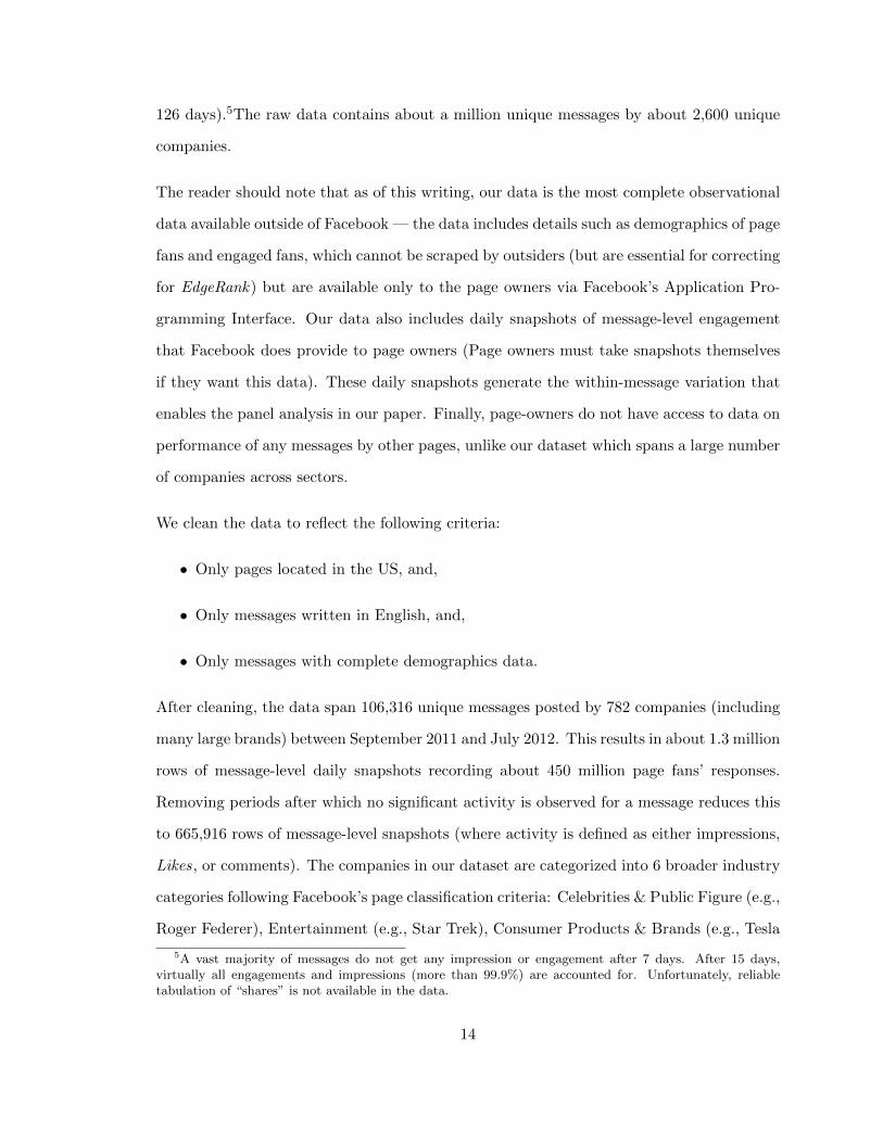
126 days).5The raw data contains about a million unique messages by about 2,600 unique
companies.
The reader should note that as of this writing, our data is the most complete observational
data available outside of Facebook — the data includes details such as demographics of page
fans and engaged fans, which cannot be scraped by outsiders (but are essential for correcting
for EdgeRank) but are available only to the page owners via Facebook’s Application Pro-
gramming Interface. Our data also includes daily snapshots of message-level engagement
that Facebook does provide to page owners (Page owners must take snapshots themselves
if they want this data). These daily snapshots generate the within-message variation that
enables the panel analysis in our paper. Finally, page-owners do not have access to data on
performance of any messages by other pages, unlike our dataset which spans a large number
of companies across sectors.
We clean the data to reflect the following criteria:
• Only pages located in the US, and,
• Only messages written in English, and,
• Only messages with complete demographics data.
After cleaning, the data span 106,316 unique messages posted by 782 companies (including
many large brands) between September 2011 and July 2012. This results in about 1.3 million
rows of message-level daily snapshots recording about 450 million page fans’ responses.
Removing periods after which no significant activity is observed for a message reduces this
to 665,916 rows of message-level snapshots (where activity is defined as either impressions,
Likes, or comments). The companies in our dataset are categorized into 6 broader industry
categories following Facebook’s page classification criteria: Celebrities & Public Figure (e.g.,
Roger Federer), Entertainment (e.g., Star Trek), Consumer Products & Brands (e.g., Tesla
5A vast majority of messages do not get any impression or engagement after 7 days. After 15 days,virtually all engagements and impressions (more than 99.9%) are accounted for. Unfortunately, reliabletabulation of “shares” is not available in the data.
14

Motors), Organizations & Company (e.g., WHO), Websites (e.g., TED), Local Places &
Businesses (e.g., MoMA).
Content-coded Data
We use a two-step method to label content. First, we contract with workers through AMT
and tag 5,000 messages for a variety of content profiles. Subsequently, we build an NLP
algorithm by combining several statistical classifiers and rule-based algorithms to extend
the content-coding to the full set of 100,000 messages. This algorithm uses the 5,000 AMT-
tagged messages as the training data-set. We describe these methods in more detail later
in the paper.
The content in Facebook messages can be categorized as informative, persuasive, or both.
Some messages inform consumers about deals and discounts about products, while other
messages seek to connect with consumers on a personal level to promote brand personality,
form relationships and are social in nature. We call the first type informative content,
and the second persuasive content. Some messages do both at the same time by including
casual banter and product information simultaneously (e.g., “Are you a tea person or a coffee
person? Get your favorite beverage from our website: http://www.specific-link-here.
com”).
Table 1 outlines the finer classification of the attributes we code up, including precise defini-
tions, summary statistics, and the source for coding the attribute. In Table 1, the 8 variables:
BRANDMENTION, DEAL, PRICECOMPARE, PRICE, TARGET, PRODAVAIL, PROD-
LOCATION, and PRODMENTION are informative. These variables enable us to assess
the effect of search attributes, brand, price, and product availability information on en-
gagement. The 8 variables: REMFACT, EMOTION, EMOTICON, HOLIDAYMENTION,
HUMOR, PHILANTHROPIC, FRIENDLIKELY, and SMALLTALK are classified as per-
suasive. These definitions include emotional content, humor, banter, and philanthropic
content.
15

Informative content variables are identified using the seminal work by Resnik and Stern
(1977), which provides an operational guideline to identify informative content. Their work
provides fourteen evaluative content criteria to identify informative content that includes
content such as product price and availability. Our persuasive content are identified mostly
from existing consumer behavior research. For example, emotional and humorous content
have been identified as drivers of word-of-mouth and of viral marketing tactics (Porter and
Golan, 2006; Berger, 2012, 2011; Berger and Milkman, 2012). Philanthropic content has
been studied in the context of advertising effectiveness (Tucker, 2012a). Similarly, Berger
and Schwartz (2011) documented that the interestingness of content such as mentions of
remarkable facts is effective in generating word-of-mouth. For a survey of papers motivating
our choice of persuasive variables, see Berger (2012). While not fully exhaustive, we have
attempted to cover most variables that are 1) highlighted by prior academic research to be
relevant, 2) commonly discussed and used in the industry.
Besides these main variables of interest, controls and content-related patterns noted as
important in industry reports are profiled. We include these content categories to inves-
tigate more formally considerations laid out in industry white papers, trade-press articles,
and blogs about the efficacy of message attributes in social media engagement. It includes
content that explicitly solicits readers to comment or includes blanks for users to fill out
(thus providing an explicit option to facilitate engagement). Additionally, characteristics
like whether the message contained photos, website links, and the types of the page-owner
(e.g., business organization versus celebrity) are also coded. Other message-specific char-
acteristics and controls include metrics such as message length in characters and SMOG
(“Simple Measure of Gobbledygook”), an automatically computed reading complexity index
that is used widely. Higher values of SMOG implies a message is harder to read. Table 2
shows sample messages taken from Walmart’s page in December 2012 and shows how we
would have tagged them. The reader should note that some elements of content tagging
and classification are necessarily subjective and based on human judgement. We discuss our
methods (which involve obtaining agreement across 9 tagging individuals) in section 2.2.2.
16

All things considered, we believe this is one of the most comprehensive attempts at tagging
marketing communication related content in the empirical literature.
Data Descriptive Graphics
This section presents descriptive statistics of the main stylized patterns in the data. The
first thing we would like to report is what kinds of content are used by firms (this may
be useful for instance, for a researcher interested in studying the role of specific content
profiles in Facebook, who would like to know what content variables are used a lot by firms).
Table 1 reports on the mean proportion of messages that have each content characteristic.
One can see that messages with videos, product or holiday mentions or emoticons are
relatively uncommon, while those with smalltalk and with information about where to
obtain the product (location/distribution attributes) are very common. Figure 2 reports
on the co-occurrence of the various attributes across messages. The patterns are intuitive.
For instance, emotional and philanthropic content co-occur often, so does emotional and
friend-like content, as well as content that describes product deals and availability. To
better describe the correlation matrix graphically and to cluster highly correlated variables
together, we ran cluster analysis to determine the optimal number of clusters using the
average silhouette width (Rousseeuw, 1987), which suggested that there are two clusters in
the data. Figure 2 shows via a solid line how content types are clustered across messages.6We
see that persuasive content types and informative content types are split into two separate
clusters, suggesting that firms typically tend to use one or the other in their messages. Later
in the paper, we show evidence suggesting that this strategy may not be optimal. Figure 3
shows the percentage of messages featuring a content attribute split by industry category.
We represent the relative percentages in each cell by the size of the bubbles in the chart.
The largest bubble is SMALLTALK for the celebrities category (60.4%) while the smallest
is PRICECOMPARE for the celebrities category (0%). This means that 6 in 10 messages by
celebrity pages in the data have some sort of small talk (banter) and/or content that does
6Clustered with hierarchical clustering.
17

Variable Description Source Mean SD Min Max
TAU (τ) Time since the post release (Day) Facebook 6.253 3.657 1 16LIKES Number of “Likes” post has obtained Facebook 48.373 1017 0 324543COMMENTS Number of “Comments” post has obtained Facebook 4.465 78.19 0 22522
IMPRESSIONS Number of times message was shown to users (unique) Facebook 9969.2 129874 1 4.5 × 10⁷
SMOG SMOG readability index (higher means harder to read) Computed 7.362 2.991 3 25.5MSGLEN Message length in characters Computed 157.41 134.54 1 6510HTTP Message contains a link Computed 0.353 0.478 0 1QUESTION Message contains questions Computed 0.358 0.479 0 1BLANK Message contains blanks (e.g. “My favorite artist is ”) Computed 0.010 0.099 0 1ASKLIKE Explicit solicitation for “Likes” (e.g. “Like if . . . ”) Computed 0.006 0.080 0 1ASKCOMMENT Explicit solicitation for “Comments” Computed 0.001 0.029 0 1
Persuasive
REMFACT Remarkable fact mentioned AMT 0.527 0.499 0 1EMOTION Any type of emotion present AMT 0.524 0.499 0 1EMOTICON Contains emoticon or net slang (approximately 1000 scraped from
web emoticon dictionary e.g. :D, LOL)Computed 0.012 0.108 0 1
HOLIDAYMENTION Mentions US Holidays Computed 0.006 0.076 0 1HUMOR Humor used AMT 0.375 0.484 0 1PHILANTHROPIC Philanthropic or activist message AMT 0.498 0.500 0 1FRIENDLIKELY Answer to question: “Are your friends on social media likely to
post message such as the shown”?AMT 0.533 0.499 0 1
SMALLTALK Contains small talk or banter (defined to be content other thanabout a product or company business)
AMT 0.852 0.355 0 1
Informative
BRANDMENTION Mentions a specific brand or organization name AMT+Comp 0.264 0.441 0 1DEAL Contains deals: any type of discounts and freebies AMT 0.620 0.485 0 1PRICECOMPARE Compares price or makes price match guarantee AMT 0.442 0.497 0 1PRICE Contains product price AMT+Comp 0.051 0.220 0 1TARGET Message is targeted towards an audience segment (e.g.
demographics, certain qualifications such as “Moms”)AMT 0.530 0.499 0 1
PRODAVAIL Contains information on product availability (e.g. stock andrelease dates)
AMT 0.557 0.497 0 1
PRODLOCATION Contains information on where to obtain product (e.g. link orphysical location)
AMT 0.690 0.463 0 1
PRODMENTION Specific product has been mentioned AMT+Comp 0.146 0.353 0 1MSGTYPE Categorical message type assigned by the Facebook Facebook– App application related messages Facebook 0.099 0.299 0 1– Link link Facebook 0.389 0.487 0 1– Photo photo Facebook 0.366 0.481 0 1– Status Update regular status update Facebook 0.140 0.347 0 1– Video video Facebook 0.005 0.070 0 1PAGECATEGORY Page category closely following Facebook’s categorization Facebook– Celebrity Singers, Actors, Athletes etc Facebook 0.056 0.230 0 1– ConsumerProduct consumer electronics, packaged goods etc Facebook 0.296 0.456 0 1– Entertainment Tv shows, movies etc Facebook 0.278 0.447 0 1– Organization non-profit organization, government, school organization Facebook 0.211 0.407 0 1– PlaceBusiness local places and businesses Facebook 0.071 0.257 0 1– Website page about a website Facebook 0.088 0.283 0 1
Table 1: Variable Descriptions and Summary for Content-coded Data: To interpret the“Source” column, note that “Facebook” means the values are obtained from Facebook,“AMT” means the values are obtained from Amazon Mechanical Turk and “Computed”means it has been either calculated or identified using online database resources and rule-based methods in which specific phrases or content (e.g. brands) are matched. Finally,“AMT+Computed” means primary data has been obtained from Amazon Mechanical Turkand it has been further augmented with online resources and rule-based methods.
18

Sample Messages Content Tags
Cheers! Let Welch’s help ring in the New Year. BRANDMENTION,SMALLTALK,HOLIDAYMENTION,EMOTION
Maria’s mission is helping veterans and their families
find employment. Like this and watch Maria’s story.
http: // walmarturl. com/ VzWFlh
PHILANTHROPIC,SMALLTALK, ASKLIKE,HTTP
On a scale from 1--10 how great was your Christmas? SMALLTALK, QUESTION,HOLIDAYMENTION
Score an iPad 3 for an iPad2 price! Now at your local
store, $50 off the iPad 3. Plus, get a $30 iTunes Gift
Card. Offer good through 12/31 or while supplies last.
PRODMENTION, DEAL,PRODLOCATION,PRODAVAIL, PRICE
They’re baaaaaack! Now get to snacking again. Find
Pringles Stix in your local Walmart.
EMOTION, PRODMENTION,BRANDMENTION,PRODLOCATION
Table 2: Examples of Messages and Their Content Tags: The messages are taken from 2012December messages on Walmart’s Facebook page.
not relate to products or brands; and that there are no messages by celebrity owned pages
that feature price comparisons. “Remarkable facts” (our definition) are posted more by
firms in the entertainment category and less by local places and businesses. Consistent with
intuition, consumer product pages and local places/businesses post the most about products
(PRODMENTION), product availability (PRODAVAIL), product location (PRODLOC),
and deals (DEAL). Emotional (EMOTION) and philanthropic (PHILAN) content have
high representation in pages classified as celebrity, organization, and websites. Similarly,
the AMT workers identify a larger portion of messages posted by celebrity, organization
and website-based pages to be similar to messages by friends.
We now discuss the engagement data. Figure 4 shows box plots of the log of impressions,
Likes, and comments versus the time (in days) since a message is released (τ). Both
comments and Likes taper off to zero after two and six days respectively. The rate of decay
of impressions is slower. Virtually all engagements and impressions (more than 99.9%) are
accounted for within 15 days of release of a message.
19

Figure 2: Co-occurrence of Attribute Characteristics Across messages. Shades in uppertriangle represent correlations. Numbers in lower triangle represent the same correlationsin numerical form in 100-s of units (range −100,+100). For e.g., the correlation in occur-rence of smalltalk and humor across messages is 0.26 (cell [3, 2]). The dark line shows theseparation into 2 clusters. Persuasive content and informative content attributes tend toform two separate clusters.
Figure 5 shows the average number of Likes and comments by message type (photo, link,
etc.) over the lifetime of a message. Messages with photos have the highest average Likes
(94.7) and comments (7.0) over their lifetime. Status updates obtain more comments (5.5)
on average than videos (4.6) but obtain less Likes than videos. Links obtain the lowest Likes
on average (19.8) as well as the lowest comments (2.2). Figure 6 shows the same bar plots
split across 6 industry categories. A consistent pattern is that messages with photos always
obtain highest Likes across industries. The figure also documents interesting heterogeneity
20

Celebrity
ConsumerProduct
Entertainment
Organization
PlacesBusiness
Websites
17 7 1 0 3 7 12 48 46 9 0 3 5 7 24 18
10 2 0 0 1 2 8 39 53 19 0 6 7 11 36 37
21 12 0 0 2 16 14 50 44 9 0 3 8 6 28 17
7 5 0 1 1 2 10 40 53 39 1 7 7 18 36 31
7 14 0 1 3 11 13 50 24 22 0 2 7 10 39 17
8 12 2 0 1 13 19 60 33 5 0 2 2 9 27 11re
mfa
ct
em
otio
n
em
otico
n
ho
liday
hu
mo
r
ph
ilan
frie
nd
like
ly
sm
allt
alk
bra
nd
me
ntio
n
de
al
pri
ce
co
mp
are
pri
ce
targ
et
pro
dava
il
pro
dlo
c
pro
dm
en
tio
n
Industry Category VS Message Content Appearance Percentage
The labels on the bubbles are the percentages
Figure 3: Bubble Chart of Broader Industry Category vs Message Content: Each bubblerepresents the percentage of messages within a row-industry that has the column-attribute.Computed for the 5000 tagged messages. Larger and lighter bubbles imply higher percentageof messages in that cell. Percentages do not add up to 100 along rows or columns as anygiven message can have multiple attributes included in it. The largest bubble (60.4%)corresponds to SMALLTALK for the celebrity page category and the smallest bubble (0%)corresponds to PRICECOMPARE for the celebrity category.
in engagement response across industries. The patterns in these plots echo those described
in reports by many market research companies such as Wildfire and comScore.
Figure 7 presents the average number of Likes and comments by content attribute. Emo-
tional messages obtain the most number of Likes followed by messages identified as “likely
to be posted by friends” (variable: FRIENDLIKELY). Emotional content also obtain the
highest number of comments on average followed by SMALLTALK and FRIENDLIKELY.
The reader should note these graphs do not account for the market-size (i.e., the number of
impressions a message reached). Later, we present an econometric model that incorporates
market-size as well as selection by Facebook’s filtering algorithm to assess user engagement
more formally.
21

0
5
10
15
1 2 3 4 5 6 7 8 9 10 11 12 13 14 15 16
Tau
Log(I
mp+
1)
Log(Imp+1) VS Tau (time since post release) boxplot
0
2
4
6
8
10
1 2 3 4 5 6 7 8 9 10 11 12 13 14 15 16
Tau
Log(C
om
ment+
1)
Log(Comment+1) VS Tau (time since post release) boxplot
0
2
4
6
8
10
12
1 2 3 4 5 6 7 8 9 10 11 12 13 14 15 16
Tau
Log(L
ike+
1)
Log(Like+1) VS Tau (time since post release) boxplot
Figure 4: Box Plots of Log(engagement+1) vs Time since message Release: Three graphsshow the box plots of (log) impressions, comments and Likes vs. τ respectively. Bothcomments and Likes taper to zero after two and six days respectively. Impressions takelonger. After 15 days, virtually all engagements and impressions (more than 99.9%) areaccounted for. There are many outliers.
22

0
20
40
60
80
link app status update video photo
Ave
rag
e C
ou
nt
comment
like
Average number of likes and comments obtained
over lifetime by message type
Figure 5: Average Likes and Comments by Message Type: This figure shows the averagenumber of Likes and comments obtained by messages over their lifetime on Facebook, splitby message type.
0
100
200
300
400
500
link app
status update
videophoto
Ave
rage C
ount
comment
like
Celebrity
0
10
20
30
40
link app
status update
videophoto
Ave
rage C
ount
comment
like
ConsumerProduct
0
20
40
60
80
100
link app
status update
videophoto
Ave
rage C
ount
comment
like
Entertainment
0
20
40
60
link app
status update
videophoto
Ave
rage C
ount
comment
like
Organization
0
5
10
link app
status update
videophoto
Ave
rage C
ount
comment
like
PlacesBusiness
0
50
100
150
link app
status update
videophoto
Ave
rage C
ount
comment
like
Websites
Figure 6: Average Likes and Comments by Message Type by Industry: This figure showsthe average number of Likes and comments obtained by messages over their lifetime splitby message type for each industry.
23

0
50
100
150
rem
fact
em
otio
n
em
otico
n
ho
liday
hu
mo
r
ph
ilan
frie
nd
like
ly
sm
allt
alk
bra
nd
me
ntio
n
de
al
pri
ce
co
mp
are
pri
ce
targ
et
pro
dava
il
pro
dlo
c
pro
dm
en
tio
n
Ave
rag
e C
ou
nt
comment
like
Average number of likes and comments obtained
over lifetime by message content
Figure 7: Average Likes and Comments by Message Content: This figure shows the averagenumber of Likes and comments obtained by messages over their lifetime split by messagecontent.
2.2.2. Amazon Mechanical Turk (AMT)
We now describe our methodology for content-coding messages using AMT. AMT is a crowd
sourcing marketplace for simple tasks such as data collection, surveys, and text analysis. It
has now been successfully leveraged in several academic papers for online data collection and
classification. To content-code our messages, we create a survey instrument comprising of a
set of binary yes/no questions we pose to workers (or “Turkers”) on AMT. To ensure high
quality responses from the Turkers, we follow several best practices identified in literature
(e.g., we obtain tags from at least 9 different Turkers choosing only those who are from
the U.S., have more than 100 completed tasks, and an approval rate more than 97%. We
also include an attention-verification question.) Please see the appendix for the final survey
instrument and the complete list of strategies implemented to ensure output quality.
Figure 8 presents the histogram of Cronbach’s Alphas, a commonly used inter-rater reliabil-
ity measure, obtained for the 5,000 messages.7The average Cronbach’s Alpha for our 5,000
7Recall, there are at least 9 Turker inputs per message. We calculate a Cronbach’s Alpha for each messageby computing the reliability across the 9 Turkers, across all the content classification tasks associated withthe message.
24

tagged messages is 0.82 (median 0.84), well above typically acceptable thresholds of 0.7.
About 87.5% of the messages obtained an alpha higher than 0.7, and 95.4% higher than
0.6. For robustness, we replicated the study with only those messages with alphas above
0.7 (4,378 messages) and found that our results are qualitatively similar.
At the end of the AMT step, approximately 2,500 distinct Turkers contributed to content-
coding 5,000 messages. This constitutes the training dataset for the NLP algorithm used
in the next step.
0
50
100
150
0.0 0.2 0.4 0.6 0.8 1.0
Cronbach’s Alpha
Counts
Cronbach’s Alphas for 5,000 Tagged
Messages Among 9+ Inputs
Figure 8: Cronbach’s Alphas for 5,000 Messages: This bar graph shows the inter-raterreliability measure of Cronbach’s Alpha among at least 9 distinct Turkers’ inputs for each5,000 messages. The mean is 0.82 and the median is 0.84. We replicated the study withonly those above 0.7 and found the result to be robust.
2.2.3. Natural Language Processing (NLP) for Attribute Tagging
We use NLP techniques to label message content from Facebook messages using the AMT-
labeled messages as the training data. Typical steps for such labeling tasks include: 1)
breaking the sentence into understandable building blocks (e.g., words or lemmas) and
identifying sentence-attributes similar to what humans do when reading; 2) obtaining a
25

set of training sentences with labels tagged from a trusted source identifying whether the
sentences do or do not have a given content profile (in our case, this source comprise the
5000 AMT-tagged messages); 3) using statistical tools to infer which sentence-attributes are
correlated with content outcomes, thereby learning to identify content in sentences. When
presented with a new set of sentences, the algorithm breaks the sentence down to building
blocks, identifies sentence-level attributes, and assigns labels using the statistical models
that were fine-tuned in the training process. We summarize our method here briefly. A
detailed description of the algorithms employed is presented in the Appendix.
The use of NLP techniques has been gaining traction in business research due to readily
available text data online (e.g., Netzer et al. (2012); Ghose et al. (2012); Geva and Zahavi
(2013)), and there are many different techniques. Our NLP methods closely mirror cutting
edge multi-step methods used in the financial services industry to automatically extract
financial information from textual sources (e.g., Hassan et al. (2011)) and are similar in
flavor to winning algorithms from the recent Netflix Prize competition.8The method we use
combines five statistical classifiers with rule-based methods via heterogeneous “ensemble
learning”. Statistical classifiers are binary classification machine learning models that take
attributes as input and output predicted classification probabilities.9Rule-based methods
usually use large data sources (a.k.a dictionaries) or use specific if-then rules inputted by
human experts, to scan through particular words or occurrences of linguistic entities in
the messages to generate a classification. For example, in identifying brand and product
mentions, we augment our AMT-tagged answers with several large lists of brands and
products from online sources and a company list database from Thomson Reuters. Further,
to increase the range of our brand name and product database, we also ran a separate
8See http://www.netflixprize.com.9We use a variety of different classifiers in this step including logistic regression with L1 regularization
(which penalizes the number of attributes and is commonly used for attribute selection for problems withmany attributes; see (Hastie et al., 2009)), Naive Bayes (a probabilistic classifier that applies Bayes theorembased on presence or absence of features), and support vector machines (a gold-standard algorithm in machinelearning that works well for high dimensional problems) with L1 and L2 regularization and various kernelsincluding linear, radial basis function, and polynomial kernels. We also utilize class-weighted classifiers andresampling method to account for imbalance in positive and negative labels.
26

AMT study with 20,000 messages in which we asked AMT Turkers to identify any brand
or product name included in the message. We added all the brand and product names we
harvested this way to our look-up database. We then utilize rule-based methods to identify
brand and product mentions by looking up these lists. Similarly, in identifying emoticons
in the messages, we use large dictionaries of text-based emoticons freely available on the
internet.
Finally, we utilize ensemble learning methods that combine classifications from the many
classifiers and rule-based algorithms we use. Combining classifiers is very powerful in the
NLP domain since a single statistical classifier cannot successfully overcome the classic
precision-recall tradeoff inherent in the classification problem. The final combined classifier
has higher precision and recall than any of the constituent classifiers.
Assessment We assess the performance of the overall NLP algorithm on three measures,
viz., accuracy, precision, and recall (as defined in Footnote 3) using 10-fold cross-validation.
10-fold cross-validation is computationally intensive and makes it harder to achieve higher
accuracy, precision and recall, but we find using the criterion critical to obtaining the
external validity required for large scale classification. Table 3 shows these metrics for dif-
ferent content profiles. The performance is extremely good and comparable to performance
achieved by the leading financial information text mining systems (Hassan et al., 2011). We
also report the improvement of the final ensemble learning method relative to using only a
support vector machine classifier. As shown, the gains from combining classifiers are very
substantial. We obtain similar results for negative class labels.
As a final point of assessment, note that several papers in the management sciences using
NLP methods implement unsupervised learning which does not require human-tagged data.
These techniques use existing databases such as WordNet (lexical database for English) or
tagged text corpus (e.g, tagged Brown Corpus) to learn content by patterns and correlations.
Supervised NLP instead utilizes human-taggers to obtain a robust set of data that can be
used to train the algorithm by examples. While unsupervised NLP is inexpensive, its
27

With Ensemble Learning Without Ensemble Learning(The Best Performing Algorithm) (Support Vector Machine
version 1 + Rule-based)
Accuracy Precision Recall Accuracy Precision Recall
REMFACT 0.94 0.99 0.68 0.88 0.99 0.33EMOTION 0.97 0.99 0.87 0.94 0.98 0.65HUMOR 0.98 1.00 0.90 0.97 1.00 0.14PHILANTHROPIC 0.97 0.99 0.85 0.93 0.99 0.62FRIENDLIKELY 0.94 0.99 0.68 0.90 0.99 0.41SMALLTALK 0.85 0.88 0.80 0.78 0.34 0.28DEAL 0.94 0.99 0.65 0.90 1.00 0.43PRICECOMPARE 0.99 0.99 1.00 0.99 1.00 0.85TARGETING 0.98 0.99 0.89 0.95 0.99 0.71PRODAVAILABILITY 0.96 0.99 0.76 0.91 1.00 0.10PRODLOCATION 0.97 0.99 0.90 0.87 1.00 0.11
Table 3: Performance of Text Mining Algorithm on 5000 Messages Using 10-fold Cross-validation: This table presents metrics for performance of the classification algorithmsused. The left 3 columns show the metrics for the final algorithm which combines classifiersvia ensemble learning methods while the right 3 columns shows the metrics for a supportvector machine algorithm. Notice that the support vector machine classifier tends to havelow recall and high precision. Naive Bayes tends to have high recall but low precision.Classifiers on their own cannot successfully overcome the standard precision-recall tradeoff(if one is higher, the other is lower). But combining many different classifiers with ensemblelearning can increase both precision and recall. We obtain similar results for negative classlabels.
performance is significantly poor compared to that of supervised NLP algorithms like the
ones implemented here. Finally, To the best of our knowledge, the NLP method used in
this paper that uses ensemble learning to combine several statistical classifiers and rule-
based methods, has not been used in business research journals.10Further, several current
implementations of NLP do not utilize the strict bar of utilizing the 10-fold cross-validation
criterion. We believe one of the contributions of this paper is to demonstrate how to utilize
AMT in combination with ensemble learning techniques, to implement supervised NLP in
business research to produce robust and cost-efficient NLP algorithms that perform well at
the scale required for empirical work. We believe the method will be useful in future studies
on unstructured natural language data such as advertising content or product reviews. For
10Although there exist business research papers combining statistical classifiers and rule-based algorithms,to our knowledge, none utilize ensemble learning methods which we find are critical in increasing accuracy,precision, and recall.
28

interested readers, a detailed step-by-step description of our NLP algorithm’s training and
classification procedures is presented in the Appendix.
2.3. Empirical Strategy
Our empirical goal is to investigate the effect of message ad content on subsequent customer
engagement. Engagement — the y-variable — is observed in the data; and content — the
x-variables — has been tagged as above and is also observed. If messages are randomly
allocated to users, the issue of assessing the effect of message-content on engagement is
straightforward; one simply projects y on x. Unfortunately, a complication arises because
Facebook’s policy of delivery of messages to users is non-random: users more likely to find
a message appealing are more likely to see the message in their newsfeed, a filtering imple-
mented via Facebook’s “EdgeRank” algorithm. The filtering implies a selection problem in
estimation of the effect of message-characteristics on engagement — if we see that messages
with photos are more likely to be commented on by users, we do not know if this is the effect
of including a photo in a message, or whether Facebook is more likely to show messages
with photos to users who are more likely to comment on them. To our knowledge, the issue
has been ignored in the literature on social media analysis so far.11We address the selection
issue via a two-step procedure, first by building a semi-parametric model of “EdgeRank”
that delivers an estimate of the expected number of impressions a message is likely to re-
ceive, and then, by incorporating this model to run a selectivity-corrected projection of
Likes and comments on message characteristics in the second-stage. For the first-stage, we
exploit the fact that we observe the aggregated decisions of Facebook to serve impressions
to users, and that “EdgeRank” is based on three variables as revealed by Facebook: Type,
Tie, and Time.12
• Type (z) refers to the type of message. Facebook categorizes message-type into 5
11We discuss later in this section why other sources of confounds (like direct targeting by firms) aresecond-order in this setting, compared to the selection induced by EdgeRank-based filtering.
12As disclosed first at the 2010 “f8” conference. See http://whatisEdgeRank.com for a brief descriptionof EdgeRank. For the duration of our data collection, this EdgeRank specification holds true.
29

classes: status update, photo, video, app, or link.
• Tie (hijt) refers to the affinity score between page j (company) and the Facebook user
i (viewer of the message) at time t which is based on the strength and frequency of
the interaction history between the user and the page.
• Time (τ) refers to the time since the message.
Our dataset contains direct observations on the variables Type and Time. We do not have
individual-level data on a user’s history with pages to model tie strengths. However, we
exploit the fact that we have access to demographics data on the set of users who could
potentially have been shown a message, versus who were actually shown the message. The
difference reflects the selection by EdgeRank, which we utilize as a proxy measure of Tie-
strength based targeting. Since we do not know the exact functional form of EdgeRank’s
targeting rule, we work with a semi-parametric specification, utilizing flexible splines to
capture the effect of EdgeRank. At the end of this step, we thus develop a flexible approx-
imation to EdgeRank’s targeting. In the second step, we can then measure the effect of
ad content on Likes and comments, by controlling for the non-random targeting using our
first-stage model. Figure 9 shows the empirical strategy visually. The advantages of directly
modeling EdgeRank this way, are that 1) we are also able to predict which message would
eventually reach users in addition to handing selection, which has auxiliary managerial value
for advertisers seeking higher reach and 2) by separating Facebook’s impression mechanism
from the effect of content on consumer engagement, we increase external validity of our
results to realms outside of Facebook Pages.
2.3.1. First-stage: Approximating EdgeRank’s Assignment
We represent message k’s type in a vector zk, the time since message k was released in τk,
and the history of user i’s past engagement with company j on Facebook in a vector hijt.
Table 4 summarizes the notation.
30

Figure 9: Impression-Engagement Funnel: Facebook’s EdgeRank chooses subset of Pagefans to show messages released by the page and fans who’ve seen the message engage withthe message based on content and type. EdgeRank is modeled with a generalized additivemodel and the final engagement is estimated through aggregate logistic regression. Detailsof estimation are in Sections 2.3.1 and 2.3.2.
Notation Description
i Userj Firmk messaget Time (day)zk message k’s media type (5 options: photo, video, status update, app, link)τk Time since message k was released
hijt History of user i’s past engagement with firm jg(.) EdgeRank score approximating function
n(d)kjt Impressions of message k by page j at time t by users in demographics bin d
N(d)jt Number of users of demographics bin d who Liked page j as of time t
θ(d)0 Intercept term for each demographics dθ(d). Parameters in EdgeRank approximation for demographics bin d
Table 4: User-level Setup Notation.
To understand our procedure, let n(d)kjt denote the number of users of demographic type
d = 1, . . . , D who were shown message k by firm j at time t. We refer to n(d)kjt as impres-
sions. We observe nkjt directly, and n(d)kjt is indirectly reported in the data and can be
reverse-engineered from Company X’s reports. Let N(d)jt denote the total number of users of
demographic type d for firm j on day t to whom the message can potentially be delivered.
N(d)jt is directly observed in the data, and comprises all users of demographics d who have
Liked the firm on Facebook. To be clear, note that Liking a message is different from Liking
31

a page — Liking a page provides the firm that maintains that page an opportunity to serve
its messages to that user via Facebook’s Newsfeed. N(d)jt is a count of all such users.
Now, note that by EdgeRank’s assignment rule, the aggregated impressions for demographic
type d, n(d)kjt, is an (unknown) function of liked-fans N(d)
jt , the tie strength between users
within demographic bucket d and the posting firm, h(d)ijt , the type of message zk, and time
since message release τk,
E(n(d)kjt) = g(N(d)
jt , h(d)ijt , zk, τk) (2.1)
We do not observe individual-level data on each users i′s interaction with every message
which could be the basis of estimating Equation (2.1). Instead, we can construct the
aggregated number of impressions and liked-fans within a set of demographic buckets in the
data. To use this variation as a source of approximating EdgeRank, we approximate the
RHS of Equation (2.1) as,
E(n(d)kjt) ≈ gd(N
(d)jt , θ
(d)1j , zk, τk) (2.2)
where, we use a firm-demographic bin specific fixed effect, θ(d)1j , to capture the effect of user
history. This approximation would literally be true if all individuals within demographic
bucket d had the same history with firm j. In practice, this is not the case, and this may
induce approximation errors into the procedure, because additional history-heterogeneity
within demographic buckets is not modeled (or is assumed into the error term). This is
a caveat to our analysis. Access to individual-level data could be the basis of improving
this procedure and relaxing this assumption. We view Equation (2.2) as a flexible approx-
imation that allows us to leverage the observed variation in firm-level impressions across
demographics, while enabling us to include firm and demographic-level fixed effects into a
procedure that best approximates EdgeRank based on what we as researchers (and firms)
know about Facebook’s filtering algorithm. We will also estimate the right-hand function
gd(.) separately for each demographic bucket, in effect allowing for slope heterogeneity in
demographics in addition to intercept heterogeneity across demographics.
32

The next step relates to approximating the function gd(.). Since we do not know the exact
functional form of the above selection equation, we approximate the function semiparamet-
rically via a Generalized Additive Model (GAM) (c.f., Hastie and Tibshirani (1990)). The
GAM is a generalized linear model with additive predictors consisting of smoothed (e.g.
interpolation and curve fitting) covariates. The GAM fits the following flexible relationship
between a set of covariates X and dependent variable Y ,
µ(E(Y |X1, X2, . . . , Xp)) = α+ s1(X1) + s2(X2) + · · ·+ sp(Xp) (2.3)
where µ is a link function (e.g. gaussian, poisson, gamma), and s1, s2, . . . sp are nonparamet-
ric smoothing functions such as cubic splines or kernel smoothers. We model the EdgeRank
selection equation for each demographic d as the following,
hd
[log(n
(d)kjt + 1)
]= θ
(d)0 + θ
(d)1j + θ
(d)2 N(d)
jt + s1(N(d)jt ; θ
(d)3 )
+5∑r=2
θ(d)4r I (zk = r) +
16∑r=2
θ(d)5r I (τk = r) + ε
(d)kjt (2.4)
where, hd ≡ g−1d (.) is the identity (Gaussian) link function, θ
(d)0 is an intercept term unique
to each demographic, d, and θ(d)1j is a firm-demographic fixed effect that captures the tie
strength between the firm j and demographics d.13N(d)jt is the number of fans of demographic
d for firm j at time t and denotes the potential audience for a message. s1 is a cubic
spline smoothing function, essentially a piecewise-defined function consisting of many cubic
polynomials joined together at regular intervals of the domain such that the fitted curve,
the first and second derivatives are continuous. We represent the interpolating function
s1 (.) as a linear combination of a set of basis functions b (.) and write: s1(N(d)jt ; θ
(d)3 ) =∑q
r=3 br
(N(d)jt
)θ
(d)3r , where the br (.) are a set of basis functions of dimension q to be chosen
13We also tried Poisson and Negative Binomial link functions (since n(d)kjt is a count variable), as well as the
identity link function without logging the y-variable. Across these specifications, we found the identity linkfunction with log (y) resulted in the best fit, possibly due to many outliers. We also considered specificationswith numerous interaction of the covariates included, but found they were either not significant or providedtrivial gains in the R2.
33

and θ(d)3. are a set of parameters to be estimated. We follow a standard method of generating
basis functions, br (.), for the cubic spline interpolation as defined in Wood (2006). Fitting
the spline also requires choosing a smoothing parameter, which we tune via generalized
cross-validation. We fit all models via the R package mgcv described in Wood (2006).
Finally, we include dummy variables for message-type (zk) and for each day since release of
the message (τk; up to 16 days), to capture the effect of message-type and time-since-release
semiparametrically. These are allowed to be d−specific. We collect the set of parameters
to be estimated for each demographic bucket in a vector, θ(d). , which we estimate by GAM
estimation. The estimated parameter vector, denoted θ(d). , d = 1, . . . , D, serves as an input
to the second stage of the estimation procedure.
2.3.2. Second-stage: Modeling Engagement Given Message Assignment
We operationalize engagement via two actions, Likes and comments on the message. The
selection problem is that users can choose to Like or comment on a message only if they are
served impressions, which generates non-random censoring because impression assignment
is endogenous to the action. We address the censoring by including a correction for the
fact that a user is shown a message non-randomly, estimated semiparametrically as above.
Suppose Ψ(d)kjt denotes the fitted estimate from the first-stage of the expected number of
impressions of message k for firm j amongst users of type d at time t,
Ψ(d)kjt = gd
(N
(d)jt , zk, τk; θ
(d))
(2.5)
We model the probability that users of type-d will Like a message given the full set of
message characteristics, Mkt, as logistic with parameters Ω = (δd, ψ)d=1,...,D,
πd(Mkt; Ω) =1
1 + e−(δd+Mktψ)(2.6)
34

The parameter vector, Ω, is the object of inference in the second stage.14
We will estimate Ω by fitting the model to explain Qkjt, the observed number of Likes of
the message in each period in the data. To see the intuition for how our correction works in
the estimation, note that we can aggregate Equation (2.6) across users, so that the expected
number of Likes is,
E(Qkjt; Ω) ≈D∑d=1
Ψ(d)kjt ×
[1
1 + e−(δd+Mktψ)
](2.7)
with Ψ(d)kjt are treated as known from the first-stage (Equation 2.5). The right-hand side is
a weighted sum of logit probabilities of Liking a message. Intuitively, the decision to Like
a message is observed by the researcher only for a subset of users who were endogenously
assigned an impression by FB. The selection functions Ψ(d)kjt serve as weights that reweigh the
probability of Liking to account for the fact that those users were endogenously sampled,
thereby correcting for the non-random nature of message assignment when estimating the
outcome equation.
We could use the expectation in Equation (2.7) as the basis of an estimation equation.
Instead, for efficiency, we estimate the parameter vector Ω by maximum likelihood. To set
up the likelihood, note the expected number of impressions of message k for firm j at time
t across all demographic buckets is simply the sum,
Ψkjt =D∑d=1
gd
(N
(d)jt , zk, τk;
ˆθ(d))
(2.8)
We can obtain an estimate of the implied probability that an impression picked at random
from the pool is of type-d,
%dkt =Ψ
(d)kjt
Ψkjt
(2.9)
14Allowing ψ to be d-specific as well in Equation (2.6) is conceptually straightforward. Unfortunately,this results in parameter proliferation and trouble with convergence; hence we settled for a more limitedspecification with d-specific intercepts.
35

Thus, the probability π (Mkt; Ω) that an impression picked at random from the pool will
Like the message given a guess of Ω, is,
π (Mkt; Ω) =D∑d=1
Pkt (d)×Pkt (Like|d) =D∑d=1
%dkt × πd(Mkt; Ω) (2.10)
Intuitively, with probability Pkt (d) = %dkt an impression is of type-d, and with probability
P (Like|d) = πd(Mkt; Ω), an impression will Like the message conditional on being type-
d; hence the unconditional probability a random impression will Like the message is the
sum-product of these marginals and conditionals across all D types.
The number of Likes is a count variable for which we specify a Binomial likelihood. Ac-
cordingly, the probability that Qkjt out of the Ψkjt assigned impressions are observed to
Like the message, and that Ψkjt − Qkjt of the remaining impressions are observed not to,
is binomial with probability, π(Mkt; Ω),
Qkjt ∼ Binomial(Ψkjt, π(Mkt; Ω)) (2.11)
Maximizing the implied binomial likelihood across all the data, treating Ψkjt as given, then
delivers estimates of Ω. The intuition for the selection correction here is the same as that
encapsulated in Equation (2.7). We can repeat the same procedure using the number of
comments on the message as the dependent variable so as the recover the effect of message-
characteristics on commenting as well. This two-step procedure thus delivers estimates of
the effects of message-characteristics on the two outcomes of interest. Standard errors are
obtained by bootstrapping both steps 1 and 2 over the entire dataset.
Discussion of Identification Identification in the model derives from two sources. First,
we exploit the observed discrepancy in demographic distributions between the set of indi-
viduals to whom a message could have been served, versus those who were actually served.
The discrepancy reflects the filtering by EdgeRank. Our first stage essentially projects this
discrepancy onto message-type, time-since-release, page and demographic characteristics in
36

a flexible way. This essentially serves as a “quasi” control function that corrects for the
selectivity in the second stage (Blundell and Powell, 2003), where we measure the effect
of message characteristics on outcomes. The second source of identification arises from
exploiting the implied restriction that the rich set of AMT-content-coded attributes affect
actual engagement, but are not directly used by EdgeRank to assign messages to users. This
serves as an implicit exclusion that helps address selection. The only message-characteristic
used by EdgeRank for assignment is zk, which is controlled for. Thus, any systematic corre-
lation in outcomes with AMT-content-coded characteristics, holding zk fixed, do not reflect
selection-related considerations. One caveat is the control for selection does depend on as-
sumptions we made about EdgeRank based on what is known publicly. We used a flexible
first-stage specification so as to be as robust as possible to these assumptions. Notwith-
standing these aspects, to the best of our knowledge, the full details of EdgeRank are not
known to any firm or researcher. In our view, a “perfect” solution to the selection problem
is unlikely to be achieved without full knowledge of Facebook’s targeting rule.
2.4. Results
2.4.1. First-Stage
The first-stage model, as specified in Equation 2.4, approximates EdgeRank’s message as-
signment algorithm. We run the model separately for each of the 14 age-gender bins used
by Facebook. These correspond to two gender and seven age bins. For a given bin, the
model relates the number of users of demographic type d who were shown message k by
firm j at time t to the message type (zk), days since message (τ), and tie between the firm
and the user. Table 5 presents the results. The intercepts (θ(d)0 ) indicate that messages by
companies in our dataset are shown most often to Females ages 35–44, Females 45–54, and
Males 25–34. The lowest number of impressions are for the 65+ age group. In our model,
tie between a user and a firm is proxied by a fixed-effect for each firm-demographic pair.
This implies 800 × 14 fixed effects corresponding to 800 firms and 14 demographic bins.
Due to space constraints, we do not present all the estimated coefficients. Table 5 presents
37

the coefficients for two randomly chosen firms. The first is a new-born clothing brand and
the second is a protein bar brand. For ease of visualization, these fixed effects are shown
graphically in Figure 10 (only the statistically significant coefficients are plotted). For mes-
sages by the the new-born clothing brand, the most impressions are among from females
in the age-groups of 25–34, 18–24, and 35–44. Among males, ages 25–34 receive the most
number of impressions. For messages by the protein bar brand, impressions are more evenly
distributed across the different demographic bins, with the Male 18–24 group receiving the
most impressions. These estimated coefficients are consistent with our expectations for the
two brands.
The estimates for message type are roughly the same in all demographic bins. For all
demographics, the photo type has the highest coefficient (around 0.25) suggesting that
photos are preferred to all other media types by EdgeRank. This is likely because users
have historically engaged better with photos causing Facebook to show photos more often.
The next most preferred message type is the status update with coefficients averaging around
0.12 followed by videos and links. The baseline message type, apps, is the message type that
is least preferred by EdgeRank. The rank ordering of coefficients for message type do not
strictly follow the rank ordering of number of messages released by firms, which is shown
in Table 1. Whereas links are posted more often, photos get more impressions relative to
messages of other types, clearly highlighting the role of EdgeRank. Days since message (τ)
are not presented in Table 5 due to space constraints. However, Figure 11 presents a box
plot of the coefficients for τ across all 14 demographic bins. All coefficients are negative and
significant and also more negative for higher values of τ , implying that EdgeRank prefers
to show more recent messages. Finally, the coefficients for number of fans, N(d)jt , are positive
and significant but they have relatively low magnitude. This is because our model includes
a smoothed term of the number of fans, s(N(d)jt ), which soaks up both the magnitude and
nonlinearity. The smoothed fan-numbers are all significant.
The generalized additive model of EdgeRank recovers coefficients that make intuitive sense
38

Female
F 13–17 F 18–24 F 25–34 F 35–44 F 45–54 F 55–64 F 65+Intercept 5.528‡ 6.071‡ 6.446‡ 7.165‡ 7.209‡ 6.133‡ 4.887‡Page 1 fixed effect –new born clothingbrand
-0.210 2.458‡ 2.685‡ 1.544† 0.888 0.813 0.489
Page 2 fixed effect –protein bar brand
-0.573‡ 1.285‡ 1.466‡ 0.928‡ 0.016 1.671‡ 1.518‡
Message Type – App is the base
Link 0.010 0.045‡ 0.063‡ 0.042‡ 0.051‡ 0.051‡ 0.048‡Photo 0.253‡ 0.318‡ 0.340‡ 0.309‡ 0.297‡ 0.267‡ 0.249‡Status Update 0.100‡ 0.161‡ 0.175‡ 0.152‡ 0.152‡ 0.129‡ 0.114‡Video 0.033 0.041 0.061† 0.041 0.021 0.024 0.030
N(d)jt (Fan Number) 2.0× 10⁻⁶‡ 1.8× 10⁻⁶‡ 7.2× 10⁻⁶‡ 1.9× 10⁻⁵‡ 1.9× 10⁻⁵‡ 3.8× 10⁻⁵‡ 8.5× 10⁻⁵‡
s(N(d)jt ) significance ‡ ‡ ‡ ‡ ‡ ‡ ‡
R-Squared 0.78 0.78 0.77 0.78 0.78 0.78 0.77
Male
M 13–17 M 18–24 M 25–34 M 35–44 M 45–54 M 55–64 M 65+Intercept 5.486‡ 6.118‡ 7.075‡ 6.635‡ 6.125‡ 5.151‡ 4.011‡Page 1 fixed effect –new born clothingbrand
0.156 0.932 1.673† 1.082 0.722 0.209 0.111
Page 2 fixed effect –protein bar brand
1.867‡ 2.423‡ 0.907‡ 0.670‡ 1.158‡ 1.575‡ 1.502‡
Message Type – App is the base
Link -0.005 0.025‡ 0.033‡ 0.034‡ 0038‡ 0.049‡ 0.030‡Photo 0.226‡ 0.284‡ 0.295‡ 0.277‡ 0.254‡ 0.230‡ 0.212‡Status Update 0.077‡ 0.124‡ 0.126‡ 0.120‡ 0.106‡ 0.103‡ 0.084‡Video 0.014 0.039 0.044* 0.031 0.016 0.007 0.023
N(d)jt (Fan Number) 3.6× 10⁻⁶‡ 1.0× 10⁻⁶‡ 6.7× 10⁻⁶‡ 2.5× 10⁻⁵‡ 3.8× 10⁻⁵‡ 5.2× 10⁻⁵‡ 2.3× 10⁻⁴‡
s(N(d)jt ) significance ‡ ‡ ‡ ‡ ‡ ‡ ‡
R-Squared 0.79 0.80 0.79 0.78 0.78 0.77 0.76
*App is the base for message type. Significance Level: ‘‡’< 0.001 ‘†’ < 0.01 ‘*’ 0.05
Table 5: EdgeRank Model Estimates: This table presents the coefficients obtained from14 generalized additive models for EdgeRank, calculated for each demographic bin. Thereare 14 demographic (gender-age) bins provided by Facebook. F13–17 means all females inthe age between 13 and 17. Time since message (τ), and page-level fixed effects are notincluded in the table and presented graphically separately.
and are consistent with claims made in several industry reports (e.g. that photos have the
highest EdgeRank weight). Further, the model fit appears to be good especially given that
we have used generalized cross-validation to guard against overfitting.
2.4.2. Second-Stage
In the second-stage, we measure the effect of content characteristics on engagement using
our selectivity-corrected model from the first-stage. All results in this section are based on
39

0
1
2
fem
ale
13
−1
7
fem
ale
18
−2
4
fem
ale
25
−3
4
fem
ale
35
−4
4
fem
ale
45
−5
4
fem
ale
55
−6
4
fem
ale
65
+
ma
le 1
3−
17
ma
le 1
8−
24
ma
le 2
5−
34
ma
le 3
5−
44
ma
le 4
5−
54
ma
le 5
5−
64
ma
le 6
5+
Pa
ge
−le
vel fixe
d−
effe
ct
fro
m G
AM
New Born Clothing Brand
Protein Bar Brand
Page−level fixed−effect estimates from GAM
across 14 demographic bins
Figure 10: Page-level Fixed effect Estimates from Generalized Additive Model Across 14Demographic Bins: This bar graph shows two randomly chosen page-level fixed effect esti-mates from the EdgeRank models. Only the statistically significant estimates are shown.New born clothing brands are positively significant for 18–24 female, 25–34 female, 35–44female, and 25–34 male. Protein bar brands have the highest fixed effect among 18–24 maledemographics.
−6
−5
−4
−3
−2
2 3 4 5 6 7 8 9 10 11 12 13 14 15 16
Tau
Co
eff
icie
nt
of
Ta
us f
rom
Ed
ge
ran
k M
od
el
Tau (time since post release) Coefficients from Edgerank Model (GAM)
Figure 11: Time Since message Release (τ) Coefficients Box plot Across Demographics:This box plot shows the coefficients on τ across all the demographics bin. τ = 1 is the basecase and every coefficients are significant at the highest level of p < 0.001.
an analysis of the entire set of over 100,000 messages (i.e. the 5,000 AMT-tagged messages as
well as the messages tagged using NLP). To present the results in a simple way, we first cre-
40
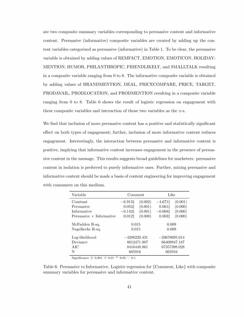
ate two composite summary variables corresponding to persuasive content and informative
content. Persuasive (informative) composite variables are created by adding up the con-
tent variables categorized as persuasive (informative) in Table 1. To be clear, the persuasive
variable is obtained by adding values of REMFACT, EMOTION, EMOTICON, HOLIDAY-
MENTION, HUMOR, PHILANTHROPIC, FRIENDLIKELY, and SMALLTALK resulting
in a composite variable ranging from 0 to 8. The informative composite variable is obtained
by adding values of BRANDMENTION, DEAL, PRICECOMPARE, PRICE, TARGET,
PRODAVAIL, PRODLOCATION, and PRODMENTION resulting in a composite variable
ranging from 0 to 8. Table 6 shows the result of logistic regression on engagement with
these composite variables and interaction of those two variables as the x-s.
We find that inclusion of more persuasive content has a positive and statistically significant
effect on both types of engagement; further, inclusion of more informative content reduces
engagement. Interestingly, the interaction between persuasive and informative content is
positive, implying that informative content increases engagement in the presence of persua-
sive content in the message. This results suggests broad guidelines for marketers: persuasive
content in isolation is preferred to purely informative ones. Further, mixing persuasive and
informative content should be made a basis of content engineering for improving engagement
with consumers on this medium.
Variable Comment Like
Constant −6.913‡ (0.002) −4.671‡ (0.001)Persuasive 0.053‡ (0.001) 0.061‡ (0.000)Informative −0.143‡ (0.001) −0.068‡ (0.000)Persuasive × Informative 0.012‡ (0.000) 0.003‡ (0.000)
McFadden R-sq. 0.015 0.009Nagelkerke R-sq. 0.015 0.009
Log-likelihood −4208220.431 −33678695.014Deviance 8012471.987 66409947.187AIC 8416448.861 67357398.028N 665916 665916
Significance ‘‡’ 0.001 ‘†’ 0.01 ‘*’ 0.05 ‘.’ 0.1
Table 6: Persuasive vs Informative: Logistic regression for Comment, Like with compositesummary variables for persuasive and informative content.
41

Table 7 presents the results of aggregate logistic regression with the full list of content
variables. We present results for both engagement metrics (Likes/comments) as well as
for models with and without the EdgeRank correction. We exclude the 16 estimated τ
coefficients from the table since they are all negative and statistically significant just as in
the EdgeRank model in Figure 11. We also exclude demographic fixed effects for space.
Scanning through the results, we observe that the estimates are directionally similar, in most
cases, with and without EdgeRank correction. However, the magnitudes often change. For
example, consider the coefficients for message type Photo. In the model without EdgeRank
correction, Photos are very likely to get comments (coefficient = 0.867) and Likes (coefficient
= 1.011). After EdgeRank correction, the results are similar but the magnitude of the effect
drops. This makes sense because we know that EdgeRank prefers Photos. Similarly, Status
Updates continue to be more likely (than apps) to get comments and Likes but the effect size
is smaller after EdgeRank correction. In some instances, there are directional changes for
some coefficients. For example, the result that links are more likely to get Likes/comments
relative to apps changes sign after EdgeRank correction. This highlights the importance
of EdgeRank correction, an issue that most industry reports (e.g., Wildfire 2012) often
overlook. For example, most industry reports’ ordering of engaging media type often list
status update to be more engaging than videos. While we find this to be true before
EdgeRank correction for Likes, we find that this is reversed after the EdgeRank correction.
We find that high reading complexity (SMOG) decreases both Likes and comments whereas
shorter messages (MSGLEN) are Liked and commented on more, albeit with a small effect
size. Having links (HTTP) is worse for engagement whereas asking questions (QUESTION)
significantly increase comments but at the cost of Likes. Using blanks in the message
to encourage comments has a similar effect of increasing comments but hurting Likes.
Interestingly, while the odds ratio of comments increases by 69% if a message asks a question,
it increases by 200% if blanks are included suggesting that blanks are more effective than
questions if the goal is to increase comments. Asking for Likes increase both Likes and
comments, whereas asking for comments increase comments but at the cost of Likes. It is
42

clear that even these simple content variables impact user engagement.
The next 16 variables in the table are the persuasive and informative content variables.
Figure 12 charts the coefficients for these variables in a bar graph and demonstrates the
sharp difference between persuasive and informative content types. Looking at comments,
a striking pattern is that most informative contents have a negative impact whereas per-
suasive contents have a positive impact. The informative content variables with the most
negative impact are PRICE, DEAL, and PRODMENTION. The persuasive content vari-
ables with the most positive impact are EMOTION and PHILANTHROPIC. Interestingly,
HOLIDAYMENTION discourages comments.15One possible explanation is that near hol-
idays, all Facebook pages indiscriminately mention holidays, leading to dulled responses.
For example, during Easter, the occurrence of holiday mention jumped to nearly 40% across
all messages released that day compared to the average occurrence of about 1%. Looking
at Likes, fewer persuasive content variables have positive impact but the results are qual-
itatively similar to that for comments. Among persuasive contents, EMOTION has the
most positive impact on Likes whereas EMOTICON has the most negative impact. Most
informative content variables continue to have a negative impact (i.e., reduce engagement),
with PRICE and DEAL having the most negative impact. The results also highlight that
there exist some differences between impact on Likes versus Comments.
Figure 13 shows the results on content effects by industry. Only the statistically signifi-
cant results are graphed and all results are EdgeRank-corrected. The coefficients are very
different across industries both in magnitude and, for some variables, in direction. For ex-
ample, emotional and philanthropic content has the most positive impact on Facebook pages
of type “Organizations” which include non-profits, educational organizations and religious
groups. Further, while mentioning holidays has a negative impact on engagement for most
industry types, it has a positive impact on engagement for Organizations. Similarly, look-
ing at informative content, we observe that variables such as Price, Product Availability,
15We checked for correlation with other contents to investigate this matter but no correlation was over0.02.
43

and Product Mentions generally have a negative impact on engagement for most industry
types, but have a positive impact for industry type “Celebrity.” Users seem more forgiving
of celebrity pages endorsing products and sharing price information.
Comparing Figures 3 and 13 also provides interesting comparisons of what each industry
is currently posting and what users engage with. For example, pages of types Places and
Businesses, Entertainment, and Consumer Products do not post emotional content much
though Figure 13 shows that emotional content induce higher Likes and Comments. Sim-
ilarly, while Places and Business pages tend to post more of deal content, only Consumer
Product pages seem to be benefiting from the deal content (in terms of obtaining more
comments). Places and Businesses pages also post larger percent of product availability
content while only the Consumer Product and Celebrity pages benefit from inclusion of
such content.
2.4.3. Robustness
Targeting by Firms
We concentrated on EdgeRank-induced selection as the main difficulty in inference since we
believe the specifics of the Facebook environment makes several other sources of confounds
second-order compared to the effect of EdgeRank. For instance, one concern may be that
firms may target content directly to specific users on Facebook. This is not possible because
in contrast to Facebook’s banner advertisements or sponsored posts, the Facebook organic
page environment does not allow companies to target specific audiences (the only factor
that can be controlled is the time-of-day of release of the message). Rather, all targeting
is implicitly implemented by Facebook via EdgeRank’s filtering. Another story may be
that firms observe that a particular type of content receives significant engagement, and
subsequently start posting similar content. Thus, new content reflects past engagement.
Our data shows significant within-variation in the attributes of messages launched over time
by a given firm, which is inconsistent with this story which would instead predict significant
44

NO ER ER NO ER ERCOMMENT OR COMMENT OR LIKE OR LIKE OR
Constant 12.309‡ (0.197) 14.083‡ (0.142) -7.383‡ (0.089) 13.504‡ (0.065)SMOG -0.045‡ (0.000) 0.956 -0.066‡ (0.000) 0.936 -0.029‡ (0.000) 0.971 -0.057‡ (0.000) 0.945MSGLEN 0.000 (0.000) 1.000 -0.000‡ (0.000) 1.000 -0.000‡ (0.000) 1.000 -0.000‡ (0.000) 1.000HTTP -0.484‡ (0.002) 0.616 -0.324‡ (0.002) 0.723 -0.353‡ (0.000) 0.703 -0.180‡ (0.000) 0.835QUESTION 0.449‡ (0.001) 1.567 0.527‡ (0.001) 1.694 -0.292‡ (0.000) 0.747 -0.185‡ (0.000) 0.831BLANK 0.942‡ (0.003) 2.565 1.099‡ (0.003) 3.001 -0.716‡ (0.002) 0.489 -0.625‡ (0.002) 0.535ASKLIKE 0.002 (0.010) 1.002 0.178‡ (0.010) 1.195 0.456‡ (0.003) 1.578 0.501‡ (0.003) 1.650ASKCOMMENT 0.779‡ (0.021) 2.179 0.710‡ (0.021) 2.034 -0.090‡ (0.011) 0.914 -0.282‡ (0.011) 0.754
Persuasive
REMFACT -0.019‡ (0.002) 0.981 0.010‡ (0.002) 1.010 -0.060‡ (0.001) 0.942 -0.035‡ (0.001) 0.966EMOTION 0.203‡ (0.002) 1.225 0.257‡ (0.002) 1.293 0.201‡ (0.001) 1.223 0.257‡ (0.001) 1.293EMOTICON 0.118‡ (0.004) 1.125 -0.053‡ (0.004) 0.948 -0.132‡ (0.001) 0.876 -0.214‡ (0.001) 0.807HOLIDAYMENTION -0.493‡ (0.014) 0.611 -0.352‡ (0.014) 0.703 -0.323‡ (0.004) 0.724 -0.136‡ (0.004) 0.873HUMOR 0.023‡ (0.002) 1.023 0.082‡ (0.002) 1.085 -0.044‡ (0.000) 0.957 0.012‡ (0.000) 1.012PHILANTHROPIC 0.147‡ (0.002) 1.158 0.140‡ (0.002) 1.150 0.008‡ (0.001) 1.008 0.001 (0.001) 1.001FRIENDLIKELY 0.002 (0.002) 1.002 -0.022‡ (0.002) 0.978 0.073‡ (0.001) 1.076 0.058‡ (0.001) 1.060SMALLTALK 0.045‡ (0.002) 1.046 -0.074‡ (0.002) 0.929 -0.052‡ (0.001) 0.949 -0.121‡ (0.001) 0.886
Informative
BRANDMENTION 0.000 (0.002) 1.000 0.077‡ (0.002) 1.080 -0.031‡ (0.000) 0.969 0.004‡ (0.000) 1.004DEAL -0.163‡ (0.002) 0.850 -0.168‡ (0.002) 0.845 -0.198‡ (0.001) 0.820 -0.200‡ (0.001) 0.819PRICECOMPARE -0.031‡ (0.001) 0.969 0.005‡ (0.001) 1.005 -0.037‡ (0.000) 0.964 -0.040‡ (0.000) 0.961PRICE -0.104‡ (0.005) 0.901 -0.319‡ (0.005) 0.727 -0.187‡ (0.001) 0.829 -0.400‡ (0.001) 0.670TARGET -0.016‡ (0.002) 0.984 -0.073‡ (0.002) 0.930 0.030‡ (0.001) 1.030 -0.041‡ (0.001) 0.960PRODAVAIL -0.067‡ (0.002) 0.935 -0.060‡ (0.002) 0.942 -0.109‡ (0.001) 0.897 -0.065‡ (0.001) 0.937PRODLOCATION -0.054‡ (0.002) 0.947 0.009‡ (0.002) 1.009 0.063‡ (0.001) 1.065 0.107‡ (0.001) 1.113PRODMENTION -0.050‡ (0.002) 0.951 -0.148‡ (0.002) 0.862 0.077‡ (0.001) 1.080 -0.007‡ (0.001) 0.993
Message Type – App is the base
– Link 0.177‡ (0.003) 1.194 -0.238‡ (0.003) 0.788 0.126‡ (0.001) 1.134 -0.374‡ (0.001) 0.688– Photo 0.867‡ (0.003) 2.380 0.519‡ (0.003) 1.680 1.011‡ (0.001) 2.748 0.651‡ (0.001) 1.917– Status Update 1.146‡ (0.003) 3.146 0.818‡ (0.003) 2.266 0.478‡ (0.001) 1.613 0.060‡ (0.001) 1.062– Video -0.106‡ (0.009) 0.899 0.466‡ (0.009) 1.594 -0.200‡ (0.003) 0.819 0.341‡ (0.003) 1.406
Industry Category – Celebrity is the base
– ConsumerProduct 0.171‡ (0.002) 1.186 -0.319‡ (0.002) 0.727 -0.369‡ (0.001) 0.691 -0.813‡ (0.001) 0.444– Entertainment 0.362‡ (0.002) 1.436 0.418‡ (0.002) 1.519 -0.291‡ (0.001) 0.748 -0.256‡ (0.001) 0.774– Organization 0.485‡ (0.002) 1.624 0.281‡ (0.002) 1.324 -0.004‡ (0.001) 0.996 -0.212‡ (0.001) 0.809– PlaceBusiness 0.429‡ (0.005) 1.536 0.021‡ (0.005) 1.021 -0.639‡ (0.002) 0.528 -1.109‡ (0.002) 0.330– Websites 0.012‡ (0.003) 1.012 0.074‡ (0.003) 1.077 0.088‡ (0.001) 1.092 0.118‡ (0.001) 1.125McFadden R-sq. 0.271 0.207 0.32 0.239Nagelkerke R-sq. 0.271 0.207 0.321 0.241Log-likelihood -2,446,467.133 -3,423,466.377 -14,108,100.91 -25,950,910.53Deviance 4,488,295.547 6,443,162.73 27,268,539.27 50,955,992.81AIC 4,893,058.266 6,847,056.753 28,216,325.82 51,901,945.06N 665,916 665,916 665,916 665,916
Significance ‘‡’ 0.001 ‘†’ 0.01 ‘*’ 0.05 ‘.’ 0.1
Table 7: Aggregate Logistic Regression Results For Comments and Likes: This tablepresents the aggregate logistic regression on comments and Likes for both EdgeRank-corrected (ER) and uncorrected (NO ER) for all data. OR means Odds ratio and showsthe odds ratio for the estimates left of the column.
45

−0.4
−0.2
0.0
0.2
rem
fact
em
otio
n
em
otico
n
ho
liday
hu
mo
r
ph
ilan
frie
nd
like
ly
sm
allt
alk
bra
nd
me
ntio
n
de
al
pri
ce
co
mp
are
pri
ce
targ
et
pro
dava
il
pro
dlo
c
pro
dm
en
tio
n
Lo
gis
tic R
eg
ressio
n C
oe
ffic
ien
ts
edgerank
no edgerank
Logistic Regression Coefficients of Message Contents for Comments
−0.4
−0.2
0.0
0.2
rem
fact
em
otio
n
em
otico
n
ho
liday
hu
mo
r
ph
ilan
frie
nd
like
ly
sm
allt
alk
bra
nd
me
ntio
n
de
al
pri
ce
co
mp
are
pri
ce
targ
et
pro
dava
il
pro
dlo
c
pro
dm
en
tio
n
Lo
gis
tic R
eg
ressio
n C
oe
ffic
ien
ts
edgerank
no edgerank
Logistic Regression Coefficients of Message Contents for Likes
Figure 12: Message Characteristic Coefficients for Comments and Likes: These bar graphsshow the coefficients of logistic regression for both EdgeRank corrected and uncorrectedmodels. Only the significant coefficients are plotted.
within-firm persistence in these attributes. Another concern is that engagement is driven by
unmeasured message characteristics that co-occur with included message characteristics. To
the extent that these unmeasured message characteristics drive engagement, they represents
unobservables that are potentially correlated with included message characteristics and
generate an omitted variables problem. This concern is plausible, but is second order in
46

−1
0
1
−1
0
1
−1
0
1
−1
0
1
−1
0
1
−1
0
1
ce
leb
rity
co
nsu
me
rpro
du
ct
en
tert
ain
me
nt
org
an
iza
tio
np
lace
sbu
sin
ess
we
bsite
SM
OG
msg
len
htt
p
qu
estio
n
bla
nk
asklik
e
askco
mm
en
t
rem
fact
em
otio
n
em
otico
n
ho
liday
hu
mo
r
ph
ilan
frie
nd
like
ly
sm
allt
alk
bra
nd
me
ntio
n
de
al
pri
ce
co
mp
are
pri
ce
targ
et
pro
dava
il
pro
dlo
c
pro
dm
en
tio
n
Typ
e:lin
k
Typ
e:p
ho
to
Typ
e:S
tatu
sU
pd
ate
Typ
e:v
ide
o
Variables
Lo
gitstic R
eg
ressio
n C
oe
f
Logistic Regression Result across Industry (Comment)
−1
0
1
−1
0
1
−1
0
1
−1
0
1
−1
0
1
−1
0
1
ce
leb
rity
co
nsu
me
rpro
du
ct
en
tert
ain
me
nt
org
an
iza
tio
np
lace
sbu
sin
ess
we
bsite
SM
OG
msg
len
htt
p
qu
estio
n
bla
nk
asklik
e
askco
mm
en
t
rem
fact
em
otio
n
em
otico
n
ho
liday
hu
mo
r
ph
ilan
frie
nd
like
ly
sm
allt
alk
bra
nd
me
ntio
n
de
al
pri
ce
co
mp
are
pri
ce
targ
et
pro
dava
il
pro
dlo
c
pro
dm
en
tio
n
Typ
e:lin
k
Typ
e:p
ho
to
Typ
e:S
tatu
sU
pd
ate
Typ
e:v
ide
o
VariablesL
og
itstic R
eg
ressio
n C
oe
f
Logistic Regression Result across Industry (Like)
Figure 13: Logistic Regression by Industry (Comments and Likes This bar graphs show thecoefficients of logistic regression for EdgeRank-corrected model. Only the significant coef-ficients (p < 0.05) are graphed. In the Like plot on the right, the coefficient for ASKCOM-MENT for websites is −4.8 but zoomed in to optimize the clarity of the graph.
our view to the extent that we have included a very rich set of message characteristics. Our
approach to this problem has been to convert unobservables into observables by collecting
direct data on a relatively comprehensive set of message-characteristics.
To validate that our results do not primarily reflect selection of certain kinds of posts by
high-performing firms, we evaluate the diversity of content posted by firms as well as serial
correlation in posts by firm. To the extent that the diversity of posts by firms is limited,
it raises the concern that certain kinds of content attributes were not used by some low
or high performing firms. Similarly, if there is high serial correlation in posts by firms, it
may reflect limited content diversity or that firms are strategically choosing posts based
on the performance of a previous post. To evaluate this issue, each post by a company is
represented by a binary vector of length sixteen (8 informative and 8 persuasive) in which
1 represents that the content attribute is present (and 0 otherwise). Next, all such vectors
47

by the same firm are simply added up to form a vector indicating overall content creation
for each firm. The Herfindahl index16is then calculated for each firm. The mean Herfindahl
index is 0.089, and the median 0.088, which is just above the minimal possible value of
116 = 0.0625. Other concentration measures, such as Gini coefficient, also report similar
patterns, which suggest that firms do mix content. Similarly, to show the extent of serial
correlation in post content released by firms, we again represent each post with a binary
vector of length sixteen. For each firm, messages are ordered by release date, then the XOR
function applied to all consecutive messages to measure content similarity. A value of 1
means that all content attributes that were used in a previous post are not present in the
current post, and vice versa. The average value of this XOR function across firms was 0.32
and the median was 0.33. This suggests significant variation in content by firms in our
dataset.
Lastly, firms may be strategic about the timing of the messages. For example, say a firm
wants to give an emotional message better exposure than a humorous message. If the firm
knows that more people are logged on Facebook at 3pm versus 8am, the firm can post the
emotional message at 3pm and the humorous one at 8am. While our model does control for
demographics and impression, if firms’ strategic targeting of specific content varies heavily
based on time of the day, this can result in vast differences in engagement across the
messages. We evaluate this possibility for all the messages in our dataset and investigate
if firms are targeting certain time of the day to post specific content. Our data show no
evidence to support this strategic timing behavior. Figure 14 presents the distribution of
the time of post for each of the sixteen content attributes. Each line represents a different
content. This graph shows that while firms are deciding when to post (such as at 5pm–6pm
when people leave their workplace), they are not posting specific content at specific time.
All distributions appear similar. In fact, none of the(
162
)pair-wise Kolmogorov-Smirnov
tests were able to reject the null that the distributions came from the same distribution.
16A measure of diversity that ranges from 1n
to 1 where 1 means highly concentrated. For our case it canrange from 1
16to 1 where 1
16means all sixteen contents are equally used.
48

The figure, coupled with high diversity of content, suggests that firms in our dataset were
not strategically selecting certain content attributes. This may be due to the lack of social
media analytics tools that provide content-level analytics. In fact, social media analytics
tools available at the data collection only provided simple timing strategies such as what
time of the day to post, as reflected in the data and controlled for in our model, but not
when to post specific content.
While it is hard to formally rule out a selection bias, all of our analysis of content diversity
and timing suggests that firms’ strategic targeting is a second order consideration for our
study.
0.02
0.04
0.06
0.08
0.10
0 5 10 15 20
Hour of the day
Pro
po
rtio
n o
f e
ach
co
nte
nt
sp
lit in
to h
ou
r−b
in Proportion of Content Split into Hour−bin
(each line represents a content)
Figure 14: Proportion of Content Posted Split into Hour-bin: Each line represents one ofsixteen content.
Alternative Specifications
We run a variety of alternative specifications to assess the robustness of our results. First,
we replicate the results using only the set of 5,000 messages directly coded up by the Amazon
Mechanical Turkers. Second, we assess the extent to which the parameters are stable when
we drop subsets of attributes. Third, we include additional checks for robustness against
selection. Our added checks use residuals from the first-stage as a “control function” in
the second-stage. To see this, note the residuals in Equation 2.4, ε(d)kjt, represent unobserved
49

reasons that users in demographic bucket d would be more likely to be targeted a message k
by EdgeRank. As robustness, we ask whether our results on the effect of message attributes
change when we control for these unobservable drivers of attractiveness of each bucket for
that message. To do this, note that from our first-stage, we can obtain an estimate of the
residual, denoted ε(d)kjt. We re-run our second stage estimation including the estimated ε
(d)kjt-s
as covariates in Mkt in Equation 2.6. We can interpret the revised results as the effect of
message characteristics on engagement after “controlling for” the unobserved attractiveness
of each bucket for that message. Results from these alternative models show that the main
qualitative features of our results are robust across these specifications.
2.5. Discussion and Managerial Implications
2.5.1. Shares, Click-throughs, and Explanation of Results
As previously mentioned, most marketers’ top goal on social media sites is to increase
consumer engagement, with the percentage of marketers who say so varying from 60% to
more than 90% across different surveys (Ascend2, 2013; Gerber, 2014; eMarketer, 2013a;
SmartBrief, 2010; Ragan and Solutions, 2012). As a result, we focused our attention on
post-level engagements — Likes and comments. However, an acknowledged limitation of
our study is that we do not have the sales data that matches the scale of 782 firms. Many
academic research (Kumar et al., 2013; Goh et al., 2013; Rishika et al., 2013; Li and Wu,
2013; Miller and Tucker, 2013; Sunghun et al., 2014; Luo and Zhang, 2013; Luo et al.,
2013) and industry reports (comScore, 2013; Chadwick-Martin-Bailey, 2010; 90octane, 2012;
HubSpot, 2013) present positive correlation and even claim causal relationships between
increased social media engagement and firm performance (e.g., purchase intention, visit
frequency, profitability, etc). This suggests that our results may extend to these other
performance measures as well. While most firms in our dataset did not track purchase
information at the post level, we additionally obtained cross-sectional data on shares and
click-throughs for the posts in our dataset to further investigate the effect of content on
50

more direct outcome measures like click-throughs.17Figure 15 show the results for shares
and click-throughs.
The results for shares are very similar to the results for comments and Likes. The general
trend of persuasive contents with positive coefficients and informative contents with negative
coefficients are replicated. Again, the emotional and humorous content were associated with
the highest level of shares, while the price and deal information were associated with the
lowest level of shares.
Results for click-throughs follow a similar trend to other engagements except for one notable
difference. The coefficients for deal information and holiday mention (which is positively
correlated with the presence of deal information) are now highly positive. While deal
information may not elicit likes, comments, and shares, we find evidence that they do
increase click-through rates. Results for other content attributes are qualitatively similar
to those for Likes and comments. The results highlight that different content has different
engagement outcomes, and that managers should implement appropriate content strategy
for their marketing goals.
2.5.2. Managerial Implications
Finally, we informally assess the extent to which the models we develop may be used as
an aid to content engineering, and to predict the expected levels of engagement for various
content profiles a firm may consider for a potential message it could serve to users. We
present an illustration set of out-of-sample prediction of engagement with real messages.
Our intent is to give the reader a rough sense for the use of our estimates as a tool to assess
expected engagement for hypothetical content bundles.
Suppose a firm’s content marketing team has developed multiple alternative messages. The
marketing team may be interested in choosing a message keeping in mind a specific engage-
ment goal. To illustrate the above, we choose three messages released around the same time
17While click-throughs do not guarantee sales, many links point to the companies’ product pages, content,and registration pages, all of which are a type of ’conversion’.
51

−0.6
−0.4
−0.2
0.0
0.2
rem
fact
emot
ion
emot
icon
holid
ay
hum
or
phila
n
frien
dlikely
smallta
lk
bran
dmen
tion
deal
pricec
ompa
re
price
targ
et
prod
avail
prod
loc
prod
men
tion
Cro
ss−
Sectional Logis
tic R
egre
ssio
n C
oeffic
ients
Share
Logistic Regression Coefficients for Shares (Cross−Sectional)
−0.4
−0.2
0.0
0.2
rem
fact
emot
ion
emot
icon
holid
ay
hum
or
phila
n
frien
dlikely
smallta
lk
bran
dmen
tion
deal
pricec
ompa
re
price
targ
et
prod
avail
prod
loc
prod
men
tion
Cro
ss−
Sectional Logis
tic R
egre
ssio
n C
oeffic
ients
Share
Logistic Regression Coefficients for Clicks (Cross−Sectional)
Figure 15: Message Characteristic Coefficients for Shares and Click-throughs: These bargraphs show the coefficients of logistic regression for EdgeRank-corrected models for Sharesand Click-throughs. Only the significant coefficients are plotted.
outside our sample. To emphasize that our second-stage model of engagement has predic-
tive power, we choose these to be for the same firm, of the same message type and having
roughly the same number of impressions (i.e., we are taking out the effect of EdgeRank).
Table 8 shows the messages, the actual lifetime engagement realized for those messages, and
the content tags we generated for those messages. For each message, we use the coefficients
from our second stage to predict the expected engagement. In the “Content Coef:” column,
we present the latent linear index of the logistic function obtained by multiplying the coef-
52
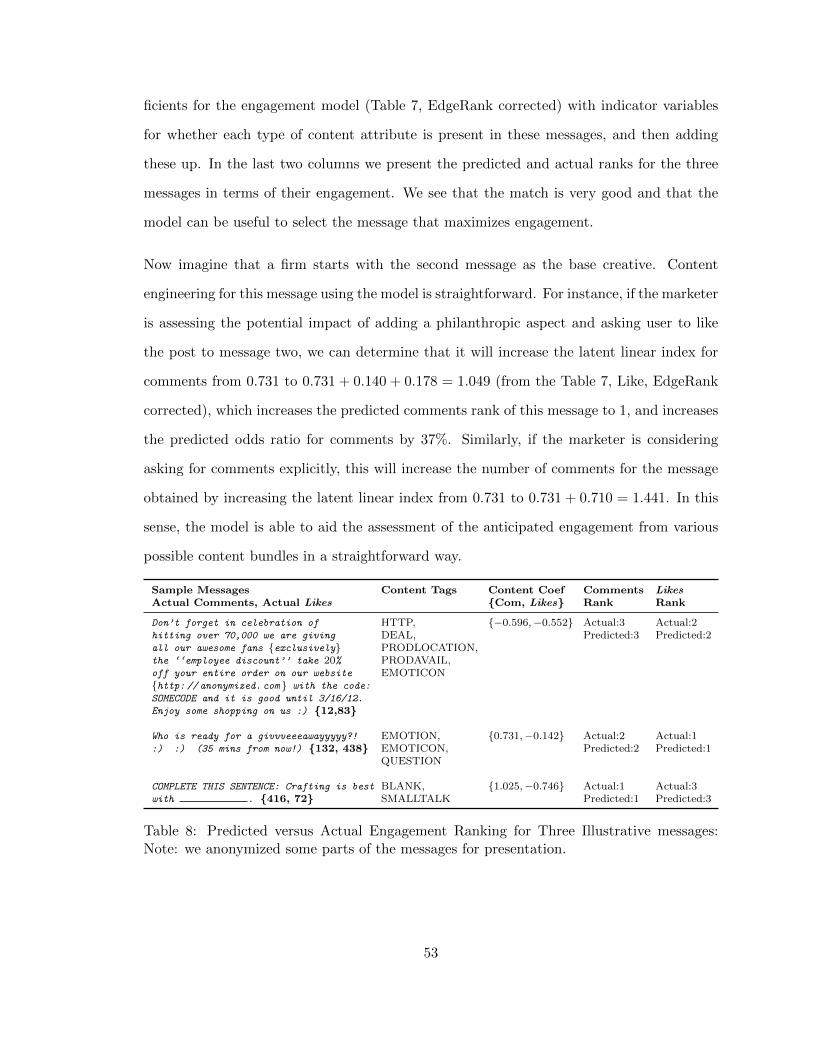
ficients for the engagement model (Table 7, EdgeRank corrected) with indicator variables
for whether each type of content attribute is present in these messages, and then adding
these up. In the last two columns we present the predicted and actual ranks for the three
messages in terms of their engagement. We see that the match is very good and that the
model can be useful to select the message that maximizes engagement.
Now imagine that a firm starts with the second message as the base creative. Content
engineering for this message using the model is straightforward. For instance, if the marketer
is assessing the potential impact of adding a philanthropic aspect and asking user to like
the post to message two, we can determine that it will increase the latent linear index for
comments from 0.731 to 0.731 + 0.140 + 0.178 = 1.049 (from the Table 7, Like, EdgeRank
corrected), which increases the predicted comments rank of this message to 1, and increases
the predicted odds ratio for comments by 37%. Similarly, if the marketer is considering
asking for comments explicitly, this will increase the number of comments for the message
obtained by increasing the latent linear index from 0.731 to 0.731 + 0.710 = 1.441. In this
sense, the model is able to aid the assessment of the anticipated engagement from various
possible content bundles in a straightforward way.
Sample MessagesActual Comments, Actual Likes
Content Tags Content CoefCom, Likes
CommentsRank
LikesRank
Don’t forget in celebration of
hitting over 70,000 we are giving
all our awesome fans exclusivelythe ‘‘employee discount’’ take 20%off your entire order on our website
http: // anonymized. com with the code:
SOMECODE and it is good until 3/16/12.
Enjoy some shopping on us :) 12,83
HTTP,DEAL,PRODLOCATION,PRODAVAIL,EMOTICON
−0.596,−0.552 Actual:3Predicted:3
Actual:2Predicted:2
Who is ready for a givvveeeawayyyyy?!
:) :) (35 mins from now!) 132, 438EMOTION,EMOTICON,QUESTION
0.731,−0.142 Actual:2Predicted:2
Actual:1Predicted:1
COMPLETE THIS SENTENCE: Crafting is best
with . 416, 72BLANK,SMALLTALK
1.025,−0.746 Actual:1Predicted:1
Actual:3Predicted:3
Table 8: Predicted versus Actual Engagement Ranking for Three Illustrative messages:Note: we anonymized some parts of the messages for presentation.
53

2.6. Conclusions
We show through a large-scale study that content engineering in social media has a sig-
nificant impact on user engagement as measured by Likes, comments, shares, and click-
throughs for messages. Our analysis shows that persuasive content, such as emotional and
philanthropic content, has a positive impact on engagement. This suggests that firms gain
from sharing their brand personality and information about their social initiatives on social
media. Further, we find that product informative content has a negative impact on user
engagement.18This presents a challenge to marketers who seek to build a large following
on social media and who seek to leverage that following to disseminate information about
new products and promotions. One takeaway from our study is that these strategies work
when product informative content is combined with persuasive content. In addition, our re-
sults are moderated by the industry type suggesting that there is no one-size-fits-all content
strategy and that firms need to test multiple content strategies.
Because of the scale of our study (nearly 800 firms and more than 100,000 messages an-
alyzed), we believe our results generalize and have broad applicability. Nonetheless, it is
important to recognize several limitation of our study. First, we note that the results from
any study on consumer response to content depend on the mix of content used in the study.
For example, we find that messages mentioning holidays, especially by consumer product
companies, have a negative effect on engagement. This may be due to excessive use of
holiday messages by firms. It is possible that the effect may be positive if firms use these
kinds of messages in moderation. Similarly, we find that emotional messages have a posi-
tive impact on engagement. Here again, it is possible this effect may reduce in the future
if firms start using emotional content excessively. Hence, it is important to interpret our
results in the context of the content mix used by firms and redo the analysis in the event
of large-scale changes in the content mix used by firms. Ultimately, we urge managers to
strike the right balance between the informative content (meant to drive leads and sales)
18With a caveat for click-throughs where a deal information was the best content.
54

and the persuasive content (meant to engage the consumers), especially since EdgeRank
uses firms’ current engagement level to determine future reach.
We used several metrics for user engagement, namely Likes and comments on messages as
well as whether users share messages with friends or visit the link in the message. Our
use of Likes, comments, shares, and click-throughs is motivated both by the widespread
use of these metrics as marketing goal in social media settings, and also the availability of
data. Future studies that evaluate other measures of interest can add value, particularly
in validating the generalizability of our findings and in exploring mechanisms underpinning
the effects we describe. As noted in the introduction, we do not address the question
of how engagement affects product demand and firm’s profits so as to complete the link
between ad-attributes and those outcome measures. Such data are still not widely available
at the scale needed for this study. Although it is not the focus of our study, it is worth
highlighting that several extant studies have studied the link between Facebook engagements
and sales (albeit at a smaller scale). For example, based on randomized studies, comScore
(2012) reports a 38% lift in purchase for fans exposed to Starbucks advertising on Facebook
through Facebook Pages or Facebook paid advertising. Similarly, studies such as Kumar
et al. (2013); Goh et al. (2013); Rishika et al. (2013); Li and Wu (2013); Miller and Tucker
(2013); Sunghun et al. (2014); Luo and Zhang (2013); Luo et al. (2013) show that social
media can be used to generate growth in sales, and ROI, consumer participation, retention,
and profitability, connecting social media metrics such as “comments” to financial metrics.
The competition for consumer attention across media outlets is intense, especially on social
media platforms. Consumers, in turn, are overwhelmed by the proliferation of online con-
tent, and it seems clear that marketers will not succeed without engineering this content for
their audience. We hope this study contributes to improve content engineering by firms on
social media sites and, more generally, creates interest in evaluating the effects of content
on consumer engagement.
55

CHAPTER 3 : People Who Liked This Study Also Liked: The Impact of
Recommender Systems on Sales Volume and Diversity
3.1. Introduction
Online consumers are constantly guided by some form of recommendation systems (RS)1,
be it for shopping or web browsing. For shopping, recommenders can be as simple as “the
most popular” items sold on the site, or as sophisticated as a collaborative filter, CF, based
on individual purchase history (e.g., Amazon.com’s “Customers who bought this item also
bought”). These systems are so pervasive in e-commerce and web services that a majority
of consumers now expect and prefer websites that provide personalized recommendations
(Accenture, 2012). At the same time, 94% of companies agree that “personalization of
the web experience is critical to current and future success” (Econsultancy and Monetate,
2013). The benefits of RS for consumers include lower search costs and higher product-fit.
In addition, with the rise of the long tail phenomenon, where in e-tailers offer a broad range
of niche items (Anderson, 2008), recommenders help consumers manage a potential choice
overload by reducing the consideration set (via showing the most relevant items). For firms,
RS has been shown to promote sales, web usage, and customer retention (Das et al., 2007;
De et al., 2010; Thompson, 2008; Monetate, 2013).
In addition to their positive impact on volume, recommenders are widely believed to affect
sales diversity. This refers to the market share distribution of products sold at the firm level
and the variety of items purchased at the individual consumer level. One school of thought
believes that recommenders lower search costs and contribute to a long tail phenomenon
in which consumers are exposed to more niche items, increasing both individual product
consumption diversity and firm-level sales diversity. An opposing theory suggests that
common recommender designs such as collaborative filters can lead to reduction in aggregate
sales diversity. It argues that because collaborative filters recommend products based on
1We use the terms recommender systems, RS, and recommender algorithms interchangeably.
56

sales and ratings, they cannot recommend items with limited historical data. This leads
to popularity bias in these designs. Understanding which viewpoint is correct is important
for retailers, consumers, and producers. For retailers whose strategy is to offer variety —
under the premise that consumers will find better-suited products and thus purchase more
— to the extent recommenders increase concentration, they may be at odds with such a
goal. Similarly for consumers and niche producers, if there exist better product matches
outside of the most popular titles, these groups may be better served (or underserved) if
these recommender systems increase sales diversity (concentration).
There are several reasons for the divergent viewpoints on the impact of RS on sales diversity.
First, a potential driver may be the lack of data that provides a contrast between users
exposed and unexposed to recommendations. Most retailers observe consumers after they
arrive at the website (i.e., after exposure to recommendations) and cannot observe the
contrast needed to answer this question. This is one reason why the question remains
empirically unanswered despite years of debate. Second, the majority of research to date has
studied specific recommender algorithms in isolation rather than comparing different kinds
of recommenders. In e-commerce, there are many types of recommenders (Schafer et al.,
1999). Most commonly used designs tend to be collaborative filtering algorithms. There can
be multiple flavors of collaborative filters, including those based on purchases (“Customers
who purchased this also purchased”) and views (“Customers who viewed this also viewed”).
Other types of recommenders include Content-based (“Based on your consumption history”)
and Social-network-based recommenders (“Your friends bought”). One possible explanation
for the divergent viewpoints is that these different recommendations have considerably
different impact on sales volume and diversity. To the extent that this is true, it alters how
firms must choose recommender designs. For example, one firm may prefer a design that
maximizes sales, whereas another firm may prefer a design that better exposes consumers
to its breadth of product assortment.
Our study attempts to address these gaps by utilizing a field experiment to examine the
57

impact of the two most commonly used recommender algorithms on sales volume and diver-
sity. By running different algorithms on the website of a top retailer in North America and
randomly assigning recommender treatments to visiting consumers and tracking their views
and purchases, we tease out the differential effects of recommender designs on both sales
volume and diversity. Our findings help answer several critical questions related to recom-
mender design. For example, is one recommender algorithm more effective for increasing
the number of products consumers view or purchase? Do certain algorithms cause “pop-
ularity bias,” wherein a top few bestsellers are promoted? How exactly do sales diversity
shift occur? What algorithms should a manager use on an e-commerce site, given product
assortment decisions and sales goals?
We find that recommender design affects both sales volume and diversity. In particular, a
collaborative filtering algorithm based on purchase data, “Customers who purchased this
item also purchased,” was best at increasing the sales volume. Further, the algorithm in-
creased individual consumption diversity but decreased aggregate consumption diversity.
We show that this differential impact in individual versus aggregate diversity is mainly
caused by users exploring into only a few ’pathway’ popular genres like comedy. The result
highlights a potential limitation in the ability of traditional collaborative filtering to aid
discovery of truly niche items and genres. We also show that not all collaborative filter-
ing algorithms are equal by contrasting the results with that for View-based collaborative
filtering.
Our results help reconcile opposing theories on the impact of recommenders using a ran-
domized field experiment. Further, they unlock important managerial insights on which
designs better address their goals. We find that collaborative filters, especially those based
on purchases, are very effective at driving an increase in sales. However, to the extent that
firms are interested in promoting a broader product assortment, we advocate that firms
should modify traditional collaborative filtering algorithms to ensure that relevant items
with limited historical sales can be discovered by consumers.
58

3.2. Prior Work
Given the significant influence of RS on e-commerce and consumer purchase behavior, the
RS literature has been growing steadily in the last couple of decades. In the 1990s, which
marked the rise of RS in e-commerce, researchers focused on developing different recom-
mender algorithms (for an extensive survey, see Adomavicius and Tuzhilin (2005)). In the
2000s, a stream of research investigated the impact of RS on sales volume, or firm perfor-
mance, looking at factors such as profit, revenue, and consumer retention (Das et al., 2007;
De et al., 2010; Thompson, 2008). In the late 2000s and 2010s, studies of RS expanded to
examining consumer consumption patterns and firm sales diversity (Fleder and Hosanagar,
2009; Hinz and Eckert, 2010; Oestreicher-Singer and Sundararajan, 2012; Jannach et al.,
2013; Matt et al., 2013; Hosanagar et al., 2014). In this section, we first provide a taxonomy
of recommender systems. Second, we review what the recommendation system literature
tells us about recommenders’ influence on sales volume and revenue, and then review the
burgeoning literature on recommenders’ influence on sales diversity. Lastly, we discuss the
gap in the literature and position our paper in it.
3.2.1. Overview and Taxonomy of Recommendation Systems
Before the advent and growth of personalized recommenders, the primary recommendation
approach used by most firms involved the use of simple signals such as the “most popular”
or “highest rated” items. A well-known current example is The New York Times’s “most
emailed articles” feature. Such signals have been shown to influence consumer learning
and choice in consumer behavior literature and in studies tied to observational learning
theory (Bikhchandani et al., 1992). Similar types of learning from the masses, whether
based on positive views or reviews, have been well documented in the literature (Salganik
et al., 2006; Muchnik et al., 2013; Tucker and Zhang, 2011; Lee et al.). While these kinds
of recommendations based on aggregate signals are privacy preserving and serve the mass
market, they may limit exploration by consumers and are less useful for consumers with
niche tastes.
59

Personalized recommenders seek to recommend items based on individual-level data. Within
Personalized Recommenders systems, a broad taxonomy distinguishes three types of algo-
rithms: Content-based, Collaborative Filtering, and Hybrid, which combines the first two
(Adomavicius and Tuzhilin, 2005). Content-based systems analyze product attributes to
suggest products that are similar to those that a consumer bought or liked in the past.
Collaborative filtering recommenders, unaware of product attributes, recommend products
either purchased or liked by similar consumers, where similarity is measured by historical
purchase (or like) data.
In recent years, social-network-based recommenders have emerged that can either simply
signal to consumers that their friends have bought certain items or can be used as an
extreme form of collaborative filtering that assumes that friends are similar in their tastes
(Victor et al., 2011). From a marketing perspective, some recent papers have looked at
how to incorporate consumers’ expressed preference and learning (Ansari et al., 2000) and
sensitivity of purchase probability (Bodapati, 2008) into recommender systems. For an
extended survey from a computer science perspective, please refer to Adomavicius and
Tuzhilin (2005).
3.2.2. Literature on the Impact of Recommenders on Sales Volume and Diversity
While there are a large number of studies on improving the actual algorithms mentioned
above, we know little about how these algorithms affect consumers and markets. While the
literature is unequivocal that recommender systems positively impact sales, it is unclear
about which designs have a greater impact. For example, industry reports have claimed
considerable increase in revenue and/or usage due to the use of recommendation systems
in the cases of Amazon, Netflix, and Google News (Thompson, 2008; Das et al., 2007;
Marshall, 2006). Recommendation engines have been reported to increase revenue up to
300%, conversion rates up to 150%, and consumers’ average order value up to 50%, according
to a recent study (Monetate, 2013). De et al. (2010) show that the use of a recommendation
system has a positive effect on the sales of both promoted and non-promoted products in
60

contrast to the use of regular search engines, which increase sales only for promoted products
and decrease sales for non-promoted products. Similarly, Hinz and Eckert (2010) show, via
agent-based modeling, that the use of recommenders can increase profits for retailers. De
et al. (2010) use a supermarket case study to show that RS increases both direct revenue
and indirect revenue, in which indirect revenue is obtained by consumers’ cross-buying
behaviors. Jannach and Hegelich (2009) carry out a case study to evaluate the use of
recommenders in a mobile app market and find that the use of RS increases click-through
rates and overall sales. In summary, there is ample evidence to support the positive effect
of RS on sales. However, the literature lacks field evidence comparing different types of
recommender algorithms and which types of designs are more effective.
Unlike the sales volume impact of RS, the sales diversity impact of RS is a subject of much
disagreement in the literature. On one side, Brynjolfsson et al. (2011) and Anderson (2008)
indicate that the use of RS will contribute to a long tail phenomenon in which niche items
gain more market share, increasing both individual- and firm-level product sales diversity.
On the other side, using theoretical models and simulations, Fleder and Hosanagar (2009)
argue that the use of collaborative filtering will lead to a decrease in firm-level aggregate
sales diversity but it can lead to an increase in individual product consumption diversity.
They suggest that collaborative filters can lead consumers to new items but aggregate di-
versity may still decrease because they push similar users to the same set of products.
Similarly, Jannach et al. (2013) use a well-known MovieLens dataset and simulation study
to show that many recommendation algorithms are biased toward broad-appeal items, caus-
ing a rich-get-richer situation that decreases aggregate product sales diversity. Celma and
Cano (2008) examine the collaborative filtering recommendation of last.fm and find that
the algorithm tends to reinforce the consumption of popular artists, supporting the hy-
pothesis that collaborative filtering will decrease aggregate diversity while also showing
that content-based algorithms are less biased toward popular artists. In contrast, Hinz and
Eckert (2010) argue through agent-based modeling that recommenders will drive a long tail
phenomenon by reducing search costs and shifting demand from broad-appeal items to niche
61

items. Echoing this idea, Oestreicher-Singer and Sundararajan (2012) argue that Amazon’s
collaborative filtering recommender (e.g., “Customers who bought this also bought”) shifts
demand from broad-appeal items to niche items, thereby increasing aggregate product sales
diversity. Similarly, regarding YouTube, Zhou et al. (2010) find evidence that the recom-
mender increases aggregate diversity. Via a lab experiment, Matt et al. (2013) argue that
both collaborative filtering and content-based recommenders increase aggregate sales di-
versity and that the differences between different recommenders are small. Similarly, by
studying a hybrid algorithm that is content-base heavy, Hosanagar et al. (2014) focus on
individual consumption patterns and show that, while recommenders increase individual
consumption diversity, they also increase commonality among consumers. They also find
that aggregate diversity increases as a result. Lastly, Wu et al. (2011) use simulation and
MovieLens data and find that content-based recommenders tend to increase the aggregate
sales diversity, while collaborative filtering decreases it. Table 9 summarizes these academic
papers and their main claims. In sum, there is no consensus among both popular and
academic literature on how recommenders will affect sales diversity.
We believe this lack of consensus arises due to the following several reasons. Some studies
evaluate one type of algorithm and are based on lab experiments or simulations calibrated
to archival data, which makes generalization harder. Other studies measure non-purchase
measure like purchase-intentions, use-intentions, and satisfaction rather than the actual
views or purchases. The few based on field archival data are aggregate level data and are
constrained by the limitations of observational data that make causal conclusions harder to
derive. We carry out a randomized field experiment on a large e-commerce website using
multiple recommender algorithms and investigate the differential effects on sales volume
and diversity with direct individual-level view and purchase data. While our approach is
not entirely free from mentioned problems, the strength of our approach is that 1) the field
experiment conducted on a large e-commerce site allows us to observe recommenders’ effects
more realistically, 2) we directly measure individual-level view and purchase data, and 3)
we have clean identification as a result.
62

Study Method & Data Sales Volume Sales Diversity
De et al. (2010) Archival Data& Econometrics
Increases sales
Hinz and Eckert (2010) MovieLens Data& Simulation
Increases sales and profit Increase niche productconsumption leading toincrease in aggregatesales diversity
De et al. (2010) Archival Data& Case Study
Increases direct andindirect revenue
Jannach and Hegelich(2009)
Mobile App Market Data& Case Study
Increases sales
Fleder and Hosanagar(2009)
Theoretical Models& Simulation
Decrease in aggregatesales diversity butincrease in individualsales diversity
Hosanagar et al. (2014) Archival Data& Econometrics
Increases individualconsumption volume
Content-based RS increaseaggregate sales diversityand increaseoverlap/commonality inconsumption
Oestreicher-Singer andSundararajan (2012)
Crawled Amazon Data& Econometrics
Increases revenue Recommender shiftsdemand to niche itemincreasing aggregatesales diversity
Jannach et al. (2013) MovieLens Data& Simulation
Different algorithms havedifferent effects
Wu et al. (2011) MovieLens Data& Simulation
Mixed result based ondifferent algorithms.Collaborative filteringdecreases aggregatediversity whilecontent-based increasesit
Celma and Cano (2008) last.fm and Allmusic.comAPI data& Correlational Analysis
Collaborative filteringalgorithm is linked topopularity bias suggestingdecreased aggregateconsumption diversity
Zhou et al. (2010) Crawled YouTube Data& Correlational Analysis
Recommender accounts for30% of video views
Increases aggregateconsumption diversity
Matt et al. (2013) Lab Experiments Increase in aggregatesales diversity forvariety of differentrecommenders exceptfor bestseller list
Table 9: Literature on Impact of Recommender Systems and Claims
63

3.3. Problem Formulation
This section formally sets up research problems and hypotheses based on the previous
literature.
3.3.1. Research Questions
We are interested in studying the impact of recommenders on sales volume and diversity.
Sales volume is measured in terms of number of purchases and value of purchases (“wallet
size”). In addition, we measure the sales diversity of the products sold with a measure
called the Gini coefficient. The Gini coefficient has been widely adopted in the long tail
and the RS literature as a measure of sales diversity (Brynjolfsson et al., 2011; Fleder and
Hosanagar, 2009; Hosanagar et al., 2014). It is computed based on the Lorenz curve. Let
L(u) be the Lorenz curve denoting the percentage of the sales generated by the lowest
100u% of items as shown in Figure 16. The Gini coefficient is defined as G ≡ AA+B . It
ranges from 0, representing the least amount of concentration or highest diversity, to 1,
representing the highest amount of concentration or lowest diversity. A Gini coefficient of 0
means that all products have equal sales, while values near 1 mean that a few broad-appeal
blockbuster items account for most of the sales.
We approach this problem with a field experiment in which consumers visiting a website are
randomly assigned to a control or treatment group. The treatment group is shown a panel
of different recommendations, much like Amazon’s “Customers who bought this item also
bought” recommenders. The control group is shown nothing. For each group, we analyze
the following variables of interest.
1. Sales Volume Impact
(a) Individual item view volume: This counts how many items individuals have
clicked and viewed.
(b) Individual item purchase volume: This counts how many items individuals
64

Figure 16: Lorenz Curve
buy. We also look at individual wallet size, which measures the total individual
purchase dollar amount.
2. Sales Diversity Impact
(a) Aggregate firm-level item (and genre) view and sales diversity: This measures
how the recommenders affect product view/sales diversity at the aggregate level
(for each treatment group) and is measured by the Gini coefficient. We repeat
this at the genre level to investigate genre cross-pollination.2
(b) Individual item (and genre) view and sales diversity: This measures how
the recommenders affect the diversity of products individuals view or purchase.
Again, the Gini coefficient is used but it is computed based on an individual’s
purchases. The analysis is repeated at the genre level.
2Measuring genres consumed is a conservative and more robust way of measuring diversity, and it isincluded in the analysis because 1) it is easier to interpret the purchase diversity of genres and 2) math-ematically, the Gini coefficient changes are more conservative at the genre level, making the results morerobust. The results are the same at the item level, with more group comparisons statistically significant.We present both in the Results section.
65

3.3.2. Treatment Groups
There are three groups in our study:
1. Control (no recommendations)
2. View-based collaborative filtering (“People who viewed this item also viewed”)
3. Purchase-based collaborative filtering (“People who purchased this item also pur-
chased”)
We have two different treatment groups corresponding to two different recommender algo-
rithms, plus a control group that was not shown any recommendations. The two treatments
are two of the most commonly used types of collaborative filtering algorithms. One is based
on views (“People who viewed this item also viewed”), while the other is based on purchases
(“People who purchased this item also purchased”). Our data partner used the widely
adopted open-source Apache Mahout framework (mahout.apache.org) for constructing the
recommenders.
3.3.3. Study Design
Let gi represent group i and let f represent a function that calculates an aggregate measure
of interest, Di, for the given group (e.g., sales volume, Gini coefficient). We define the
following quantity of interest:
Aggregate Measure, f , of Group 1 D1 ≡ f(g1)
Aggregate Measure, f , of Group 2 D2 ≡ f(g2)
Difference in Aggregate Measures D ≡ D1 −D2
The difference in the aggregate measure, D, shows how different Group 1 is from Group 2.
Let µ ≡ E[D], with the distribution of D unknown. All hypotheses testing in this paper
takes the form:
66

Null Hypothesis H0 µ ≡ E[D] = 0
Alternate Hypothesis Ha µ ≡ E[D] 6= 0
This null hypothesis tests if variables of interest, such as group revenues for Groups 1 and
2, are distributed equally. Since we have one aggregate measure (or statistic) for each
group, in order to produce a p-value, we utilize a permutation test technique (Good, 2005)
that allows us to calculate a null distribution for a given aggregate measure. If the null
hypothesis of equal distribution is true, all relabelings of individuals as Groups 1 and 2 are
equally likely. A permutation test involves repeatedly and randomly relabeling individuals
into Groups 1 and 2 (e.g., control and treated) to produce a null distributions for any test
statistics. By comparing statistics from null distributions to the actual test statistics from
the real distribution and tallying how often null distribution statistics exceed the actual
distribution statistic, we can determine the p-value. For more details, see Good (2005).
Note that we carry out the hypotheses tests as two-sided tests (equal or not equal rather
than greater than or less than) to stay conservative. In our study, we use 1000 iterations to
get an accurate p-value up to 0.001.
3.3.4. Hypotheses
We organize our hypotheses on the impact of recommenders on sales volume and diversity in
this section. Our hypotheses are informed by the extant literature discussed in Section 3.2.
While the hypotheses on sales volume are clearly driven by unequivocal results of previous
studies, we take a particular stance on sales diversity since the existing literature disagrees
on this matter.
Sales Volume Hypotheses There appear to be many reasons why recommenders affect
sales volume. Many long tail and recommender studies (Brynjolfsson et al., 2006, 2011;
Oestreicher-Singer and Sundararajan, 2012; Hinz and Eckert, 2010) postulate that person-
alized recommenders reduce consumers’ search costs by reducing the need to search for the
right product. In doing so, recommenders make it easy for consumers to find the right prod-
67

ucts, which leads to more purchases. The impact on number of product views is less clear.
On the one hand, a reduction in search cost can lead consumers to their desired product
faster, resulting in fewer clicks and product views. On the other hand, recommenders may
be effective in cross-selling, up-selling, or even in driving repeat visits, thereby resulting in
increase in number of product views. We hypothesize that recommenders will contribute
toward an increase in purchases as well as product views.
Hypothesis 1 Collaborative filtering (CF) recommenders will increase the number of
product views compared to no recommendation condition (Control).
Hypothesis 2 Collaborative filtering (CF) recommenders will increase the number of
product purchases compared to no recommendation condition (Control).
Although we have two different types of collaborative filters (Purchase-based or View-
based), we do not make any hypotheses comparing the two. Intuition suggests that collab-
orative filtering based on purchase data will be more potent, since a purchase is a stronger
signal than a view and is probably more accurate.
Sales Diversity Hypotheses Fleder and Hosanagar (2009) offer a clear conjecture on
how collaborative filters affect product consumption diversity at both the aggregate and
individual level. They argue that a collaborative filtering algorithm will show popularity
bias by directing users to broad-appeal blockbuster items, leading to decreased aggregate
firm-level product sales diversity. Likewise, Celma and Cano (2008) and Wu et al. (2011)
also support the hypothesis that collaborative filtering will decrease aggregate product
sales diversity. At the same time, Fleder and Hosanagar (2009) predict that individuals
will be exposed to a greater variety of products, leading to increased individual product
consumption diversity. Our hypotheses on sales diversity are based on the Fleder and
Hosanagar (2009) paper, which presents a theoretical model specifically on collaborative
filtering and provides conjecture on both the aggregate and individual diversity.
In summary, our hypotheses on the sales diversity impact of RS are as follows:
Hypothesis 3 Collaborative filtering recommenders will decrease the aggregate product
68

sales diversity compared to no recommendation condition (control), i.e., Aggregate Gini(CF)
> Aggregate Gini(Control).
Hypothesis 4 Collaborative filtering recommenders will increase the individual prod-
uct purchase diversity compared to no recommendation condition (control), i.e., Average
Individual Gini(CF) < Average Individual Gini (Control).
3.4. Data
Our dataset comes from a field experiment on a website of one of the top retailers in North
America. The experiment was conducted for two weeks between August 8, 2013 and August
22, 2013. Focusing attention on a product category commonly used in the RS literature,
this study examines the impact of recommenders on movie-related (Blu-ray disc and DVD)
product views and purchases. The field experiment was run by the company using a state-of-
the-art A/B/n testing platform. This platform implemented a session tracking technology
whereby each visitor’s IP address is recorded and given a unique visitor ID. Then visitors’
behaviors are tracked over the period of the field experiment. This enables the website to
track individuals’ viewing logs and purchases over many days. Whenever new visitors access
the website for the first time, they are randomly chosen to be in the control or one of the
treatment groups. Upon clicking and viewing a particular item, the visitors are shown the
appropriate recommender panel, as seen in Figure 17. Figure 17 is a collaborative filtering
recommender based on views (“People who viewed this item also viewed”). Similarly, there
is also a collaborative filtering based on purchases, as mentioned in Section 3.3.2. Users
in the control group do not see this panel. At the end of the experiment, we have each
consumer’s view logs and purchase logs at the item level. The algorithms were retrained
every three days to propagate the influence of users’ purchase history multiple times over the
period of the experiment. About half of the users in the dataset were returning users. The
website provides its own movie categorization, but in order to make the genre categorization
more robust, we categorize each movie using IMDB.com’s3categorization. For each movie,
3World’s top movie information website, according to Alexa rank.
69

we obtain IMDB.com’s category information by asking at least three different users on
Amazon Mechanical Turk (“Turkers”) to provide primary genres from IMDB.com. Getting
input from three Turkers ensures robustness, which is important in even this simplest look-
up-and-copy/paste task. Table 10 shows each genre’s product page views and purchase
numbers. All data were anonymized to ensure privacy.
Figure 17: Recommender Example: Example of a recommender shown to a consumer. Thisconsumer was in the treatment group of collaborative filtering based on views.
When the company ran the field experiment, it wanted to test the recommenders with a
very small fraction of its visitors since the company had never used recommenders on this
particular website. Therefore, it randomly allocated 10% of its visitors to each collaborative
filtering treatment group. Our analysis focuses on only those users who made at least
one purchase during the study period. This is because it does not make as much sense
to compute individual-level sales diversity measures (like the Gini coefficient) when no
purchases have been made by the individual. There is no selection bias in this case since,
ex ante, we randomized the treatment and control assignments for all visitors. A caveat to
our study is that we investigate the effects on only those consumers who ended up making a
purchase. Our resulting dataset has 572 unique users in the control group and about 70 to
70

Viewed PurchasedGenres Genres
Action 625 291Adventure 114 50Animation 557 240Biography 21 13Comedy 565 282Crime 41 22Documentary 48 31Drama 465 217Family 321 127Fantasy 65 41History 1 0Horror 96 25Music 4 1Musical 29 19Mystery 9 6Romance 38 20Sci Fi 169 80Sport 181 79Thriller 39 20War 17 6Western 17 6
Table 10: Movie Genres Viewed and Purchased: This table shows the number of views andpurchases in each movie genres in our dataset for those who’ve viewed or purchased movies(DVDs, Blu-ray discs) on this e-commerce site.
90 who purchased movie-related products in each of the other groups. Multiple robustness
checks that account for sample size differences and outliers are presented in Section 3.5.6,
and all checks produced similar results.
Our field experiment dataset offers a clean way to tease out the causal impact of recom-
menders. However, it is lacking in that we do not consider all recommender designs used
in practice, such as content-based recommenders. However, given that much of the debate
in the recommendation systems literature relates to collaborative filters, we have the two
most commonly used designs in our study.
71
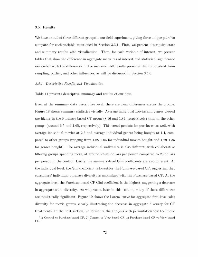
3.5. Results
We have a total of three different groups in our field experiment, giving three unique pairs4to
compare for each variable mentioned in Section 3.3.1. First, we present descriptive stats
and summary results with visualization. Then, for each variable of interest, we present
tables that show the difference in aggregate measures of interest and statistical significance
associated with the differences in the measure. All results presented here are robust from
sampling, outlier, and other influences, as will be discussed in Section 3.5.6.
3.5.1. Descriptive Results and Visualization
Table 11 presents descriptive summary and results of our data.
Even at the summary data descriptive level, there are clear differences across the groups.
Figure 18 shows summary statistics visually. Average individual movies and genres viewed
are higher in the Purchase-based CF group (8.16 and 1.84, respectively) than in the other
groups (around 6.5 and 1.65, respectively). This trend persists for purchases as well, with
average individual movies at 2.5 and average individual genres being bought at 1.4, com-
pared to other groups (ranging from 1.88–2.05 for individual movies bought and 1.29–1.35
for genres bought). The average individual wallet size is also different, with collaborative
filtering groups spending more, at around 27–28 dollars per person compared to 25 dollars
per person in the control. Lastly, the summary-level Gini coefficients are also different. At
the individual level, the Gini coefficient is lowest for the Purchase-based CF, suggesting that
consumers’ individual-purchase diversity is maximized with the Purchase-based CF. At the
aggregate level, the Purchase-based CF Gini coefficient is the highest, suggesting a decrease
in aggregate sales diversity. As we present later in this section, many of these differences
are statistically significant. Figure 19 shows the Lorenz curve for aggregate firm-level sales
diversity for movie genres, clearly illustrating the decrease in aggregate diversity for CF
treatments. In the next section, we formalize the analysis with permutation test technique
41) Control vs Purchase-based CF, 2) Control vs View-based CF, 3) Purchase-based CF vs View-basedCF.
72

View Control View-based CF Purchase-based CF
Unique ConsumersWho Purchased Movie Products
572 73 95
Average IndividualMovie Genres Viewed
1.65 (1.37) 1.67 (1.31) 1.84 (1.85)
Average Individual Movies Viewed 6.54 (8.64) 6.75 (7.39) 8.16 (13.70)
Number of ConsumersViewing More than 1 Movie
489 62 81
% of ConsumersViewing More than 1 Movie
0.851 0.849 0.852
Average Individual MovieGini Coefficient
0.9988 (0.0016) 0.9988 (0.0011) 0.9983 (0.0045)
Average Individual GenreGini Coefficient
0.9338 (0.0358) 0.9315 (0.0423) 0.9299 (0.0425)
Aggregate Genre Gini Coefficient 0.6262 0.6476 0.6772
(a) Summary Statistics for View
Purchase Control View-based CF Purchase-based CF
Unique ConsumersWho Purchased Movie Products
572 73 95
Average IndividualMovie Genres Bought
1.29 (0.85) 1.35 (0.75) 1.41 (1.20)
Average Individual Movies Bought 1.88 (2.29) 2.05 (1.41) 2.54 (7.83)
Average Individual Wallet Size 24.97 (32.01) 27.84 (24.59) 27.27 (51.67)
Number of ConsumersBuying More than 1 Movie
186 35 34
% of ConsumersBuying More than 1 Movie
0.325 0.479 0.357
Average Individual MovieGini Coefficient
0.9985 (0.0018) 0.9984 (0.0011) 0.9979 (0.0062)
Average Individual GenreGini Coefficient
0.9418 (0.0277) 0.9390 (0.0308) 0.9389 (0.0325)
Aggregate Genre Gini Coefficient 0.6076 0.6768 0.7044
(b) Summary Stat for Purchase
Table 11: Data Summary Statistics: Standard deviation is in parentheses
73

2
3
4
5
6
7
8
View Purchase
Ave
rag
e I
nd
ivid
ua
l M
ovie
Ite
ms P
urc
ha
se
d
Control
View−Based CF
Purchase−Based CF
Average Number of Movies Viewed or
Purchased by Individuals
(a) Average Individual MoviesViewed/Purchased
1.2
1.3
1.4
1.5
1.6
1.7
1.8
View Purchase
Ave
rag
e I
nd
ivid
ua
l M
ovie
Ge
nre
s P
urc
ha
se
d
Control
View−Based CF
Purchase−Based CF
Average number of genres viewed or
purchased by individuals
(b) Average Individual GenresViewed/Purchased
24
25
26
27
28
Control View−Based CF Purchase−Based CF
Ave
rag
e I
nd
ivid
ua
l W
alle
t S
ize
(To
tal $
Sp
en
t)
Average Wallet Size Per Individual
(c) Average Individual Wallet Size
0.925
0.930
0.935
0.940
View Purchase
Ave
rag
e I
nd
ivid
ua
l G
en
re G
ini
Control
View−Based CF
Purchase−Based CF
Average Gini of Genres Viewed or
Purchased by Individuals
(d) Average Individual Genre Gini
Figure 18: Average Individual Statistics: These graphs visualizes the average individualnumber of movies viewed/purchased, wallet size (total $ spent), and the Gini measure ofgenres viewed/purchased.
and provide group-level differences for each variable of interest with statistical significance.
3.5.2. Sales Volume Results
Individual Item Views Table 12 summarizes the results for the average number of items
viewed per individual. The top rows present the average number of items viewed in each
74

0.0 0.2 0.4 0.6 0.8 1.00.0
0.2
0.4
0.6
0.8
1.0
Aggregate Genre Purchase Diversity
Lorenz Curve for View−Based CF
Cumulative % of movie genres
Cum
ula
tive
% o
f purc
hase
0.0 0.2 0.4 0.6 0.8 1.00.0
0.2
0.4
0.6
0.8
1.0
Control
View−Based CF
0.0 0.2 0.4 0.6 0.8 1.00.0
0.2
0.4
0.6
0.8
1.0
Aggregate Genre Purchase Diversity
Lorenz Curve for Purchase−Based CF
Cumulative % of movie genres
Cum
ula
tive
% o
f purc
hase
0.0 0.2 0.4 0.6 0.8 1.00.0
0.2
0.4
0.6
0.8
1.0
Control
Purchase−Based CF
Figure 19: Lorenz Curves for Movie Genres Purchased: These Lorenz curves show that,on the genre level, firm-level aggregate sales diversity is decreased for both collaborativefiltering algorithms.
group and the difference relative to the control group. The remaining cells evaluate whether
the difference between two groups is statistically significant or not. The test statistic is D ≡
f(grow)−f(gcolumn) with f representing the average number of items viewed by individuals
in a group; grow refers to the group identified in that row. The test statistic is followed by
the p-value associated with the value. The p-value is computed using a permutation test as
outlined above. For example, consumers in the control group on average viewed 6.54 items,
while View-based-CF-exposed consumers viewed 6.75 items. The difference between the two
is −0.2070, and the p-value associated with this difference statistic D is 0.796. Consumers
treated with the Purchase-based CF viewed 1.6 more items on average (a 25% lift) compared
to the control, and this difference is statistically significant. The Purchase-based CF also
performs better than the View-based CF, which only lifts views by 3% compared to the
control. It is clear that 1) CFs can increase exploration on e-commerce sites, and 2) there
is a difference between CF algorithms in terms of their impact on product views. The
success of the Purchase-based CF may be because they help broaden the consideration set
by recommending other relevant alternatives or because they are effective at cross-selling
other product categories. The former may not necessarily create new purchases even if it
75

helps improve product match for consumers, whereas the latter should contribute towards
new purchases.
Avg # of Items Viewed 6.5464 6.7534 8.1684% Change from Control 3.1% N 24.7% N
Control View-based CF Purchase-based CFControl −0.2070|0.796 −1.6220|0.026
View-based CF −1.4149|0.402Row − Column|P -value
Table 12: Individual Item Views Comparison: Individual items (movies) viewed averagedwithin each group. The top row shows the actual average items viewed in each group. Eachcell shows a ROW−COLUMN value with p-value (e.g., Average items viewed in control —average items viewed in View-based CF = −0.2070 and p-value obtained from permutationtest is equal to 0.796).
Individual Item Purchases Table 13 presents the same information for item purchases.
The impact of the treatments on purchases is directionally similar to their impact on views.
The Purchase-based CF is the only group that is statistically significantly different from
the control group. Consumers bought 0.66 more items on average (a 35% lift) under the
influence of the Purchase-based CF than the control group. Consumers in the View-based
CF group bought 0.17 more items on average (a 9% lift) than consumers in the control group
(the difference is not statistically significant). The results again validate that CF can have
a significant impact on purchases and that there are differences between CF algorithms.
Further, we find that the Purchase-based CF is effective in creating new purchases.
Avg # of Items Purchased 1.8809 2.0547 2.5473% Change from Control 9.2% N 35.4% N
Control View-based CF Purchase-based CFControl −0.1738|0.342 −0.6664|0.004
View-based CF −0.4925|0.932
Table 13: Individual Item Purchases Comparison: Individual items (movies) purchasedaveraged within each group.
Individual Wallet Size Table 14 shows that, while nothing is statistically significant in
the individual wallet-size comparison, CF average wallet sizes were higher than the control’s.
Both CF groups yielded an average wallet size above $27 per person. The control group
76

yielded the smallest average wallet size, coming up just below $25.
Avg Wallet Size 24.9761 27.8473 27.2794% Change from Control 11.4% N 9.2% N
Control View-based CF Purchase-based CFControl −2.8712|0.296 −2.3033|0.416
View-based CF 0.5679|0.946
Table 14: Individual Wallet-Size Comparison: Individual Wallet Size (total amount spent)averaged within each group.
Discussion Our results on the sales volume impact of recommenders are clear. Purchase-
based CF exposes users to more items, and in fact, increases the sales volume. Specifically,
Purchase-based CF drives a 25% lift in views and a 35% lift in the number of items purchased
compared to the control group. In comparison, the View-based-CF group shows only a 3%
lift in views and a 9% lift in the number of items purchased, which is not statistically
significant. While the wallet-size analysis was not statistically significant, it suggests that
CFs do increase the amount spent by consumers. It is highly likely that the lack of statistical
significance is driven by the fact that purchases were infrequent and our data spans only a
two-week period.
3.5.3. Sales Diversity Results
Aggregate View Diversity Table 15 shows the aggregate view diversity at the item
and genre levels for the three groups. At the item level, both treated groups decrease
in view diversity (i.e., increased Gini), and the results are statistically significant. Users
as a whole view fewer items when shown collaborative filtering recommendations. At the
genre level, only the Purchase-based collaborative filter decreased view diversity statistically
significantly compared to the control group. The results stay the same when the analysis is
repeated by first fixing the same number of randomly sampled users in each group instead
of permuting with the entire sample.
Aggregate Sales Diversity Table 16 presents the first part of our main results on the
sales diversity impact. Subtables 16a-16b show the impact of each recommender algorithm
77

Aggregate View GiniItem
0.6312 0.9374 0.8921
% Change from Control 48.5% N 41.3% N
Control View-based CF Purchase-based CFControl −0.3061| < 0.001 −0.2608| < 0.001
View-based CF −0.0452|0.1(a) Aggregate Item View Diversity Comparison
Aggregate View GiniGenre
0.6262 0.6476 0.6772
% Change from Control 3.4% N 8.1% N
Control View-based CF Purchase-based CFControl −0.0214|0.390 −0.0509|0.042
View-based CF −0.0295|0.470
(b) Aggregate Genre View Diversity Comparison
Table 15: Aggregate View Diversity
Aggregate PurchaseGini Item
0.3972 0.8907 0.8235
% Change from Control 124.2% N 107.4% N
Control View-based CF Purchase-based CFControl −0.4935| < 0.001 −0.4262| < 0.001
View-based CF 0.0672|0.306
(a) Aggregate Item Sales Diversity Comparison
Aggregate PurchaseGini Genre
0.6076 0.6768 0.7044
% Change from Control 11.3% N 15.9% N
Control View-based CF Purchase-based CFControl −0.0691|0.004 −0.0967| < 0.001
View-based CF −0.0276|0.392
(b) Aggregate Genre Sales Diversity Comparison
Table 16: Aggregate Sales Diversity
on aggregate sales diversity at the item and genre levels, respectively. At the item level,
both treated groups show a statistically significant reduction in aggregate sales diversity.
In tandem with the results from the aggregate view diversity, we see that for both treated
groups, consumers as a group explored and purchased a less wide variety of items. Users
in the treated groups ended up buying the same broad-appeal items, leading to some level
of herding. This popularity bias persists at the genre level. These results support the
theoretical results presented in Fleder and Hosanagar (2009) that conjecture that typical
78

collaborative filtering designs will show a popularity bias at the aggregate level because
they make recommendations based on past purchases and/or views.
Tables 15 and 16 also show some differences in terms of how recommenders influence item
diversity versus genre diversity. Collaborative filtering algorithms seem to cause heavier
shifts in item diversity than in genre diversity both in percentage and absolute terms. This
is in part due to the number of items, which are order of magnitude greater than the number
of genres, thereby amplifying the effect of popularity bias of recommenders. Collectively,
these tables suggest that CF algorithms change view and purchase diversity both at the
item and genre level, but more so at the item level.
Individual View GiniItem
0.9988 0.9988 0.9983
% Change from Control 0% 0.05% H
Control View-based CF Purchase-based CFControl 0.00001|0.934 0.0004| < 0.001
View-based CF 0.0004|0.482
(a) Individual Item View Diversity Comparison
Individual View GiniGenre
0.9338 0.9315 0.9299
% Change from Control 0.2% H 0.4% H
Control View-based CF Purchase-based CFControl 0.0022|0.408 0.0039|0.164
View-based CF 0.0016|0.814
(b) Individual Genre View Diversity Comparison
Table 17: Individual View Diversity
Individual View Diversity Table 17 presents results for individual view diversity. The
only statistically significant result is at the item level with the Purchase-based CF algorithm.
The Purchase-based CF causes individual view diversity to increase (i.e., the Gini coeffi-
cient is lower than that of the control). Unlike aggregate view diversity, which decreases,
individual view diversity increases. This means that individuals view a greater variety of
items while consumers as a group view a more limited variety of items. While puzzling, this
result is explained by Fleder and Hosanagar’s (2009) theory that recommenders “can push
each person to new products, but they often push users toward the same products” because
79

one person’s product views or purchases feed into recommendations made to another user.
Individual PurchaseGini Item
0.9985 0.9984 0.9979
% Change from Control 0.01% H 0.06% H
Control View-based CF Purchase-based CFControl 0.0001|0.426 0.0005|0.002
View-based CF 0.0004|0.946
(a) Individual Item Purchase Diversity Comparison
Individual PurchaseGini Genre
0.9418 0.9390 0.9389
% Change from Control 0.2% H 0.3% H
Control View-based CF Purchase-based CFControl 0.0028|0.184 0.0029|0.206
View-based CF 0.00008|0.996
(b) Individual Genre Purchase Diversity Compariso
Table 18: Individual Purchase Diversity
Individual Purchase Diversity Table 18 shows the results for individual purchase di-
versity. Similar to the individual view diversity, individual purchase diversity increases (i.e.,
the Gini coefficient decreases), suggesting that individuals buy a greater variety of items
because of exposure to Purchase-based collaborative filtering recommenders. The directions
for genre are the same but are not statistically significant.
Looking at Tables 15–18, we see a clear pattern emerging. Under the influence of the
Purchase-based CF, individuals view and buy a greater variety of items than under no
recommenders, but they collectively discover and buy a similar set of items, leading to a
decrease in aggregate view and sales diversity. The View-based CF shows similar results
but the effect sizes are smaller and sometimes not statistically significant. This suggest
that, even within collaborative filtering algorithms, there are differences. Our results further
show that recommenders influence both the consideration set (views) as well as the eventual
conversion (purchase).
80

3.5.4. Results Summary
Table 19 summarizes our results and hypotheses supported. Our results confirm anecdotal
and industry reports of the sales volume impact of the recommenders, specifically for the
collaborative filtering algorithms. Collaborative filtering increases both the number of prod-
uct (in this case, DVD and Blu-ray) views and the number of items purchased, suggesting
that these recommenders can successfully engage users in additional search and exploration
and eventually additional purchases. Further, we show that not all collaborative filtering
algorithms perform the same. In our setting, Purchase-based collaborative filters had a
more significant impact on sales than View-based filters.
Regarding the sales diversity impact of recommenders, we have shown that collaborative
filtering causes individuals to discover a greater variety of products but pushes consumers to
the same set of titles, leading to concentration bias at the aggregate level. Here again, we find
that not all collaborative filtering algorithms are the same. Purchase-based collaborative
filters have a greater impact. This may be because: 1) the algorithm based on purchases
might simply be better at delivering the best fit products, 2) consumers might be more
influenced by the “purchased also purchased” signal than the “view also viewed” signal,
3) or both. However, we lack the access to detailed recommender data and consumer
information to deeper investigate and quantify which of these effects are in play5.However,
in the next section, 3.5.5, we investigate the source of diversity shift at the genre level,
providing further insight into how the increase in individual diversity and the decrease in
aggregate diversity can occur simultaneously.
3.5.5. The Source of Diversity Shift: Genre Cross-pollination Investigation
In this section, we attempt to visualize our results and also understand from where the shift
in aggregate and individual diversity stems. To do so, we construct sample-size normalized
genre-level co-purchase networks for both Purchase-based CF and the control. We create
5We believe that investigating and quantifying the two underlying recommender mechanism is a promisingand interesting line of study.
81
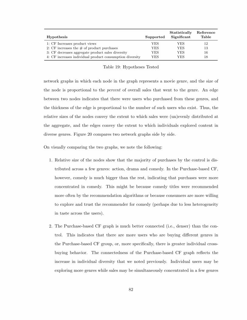
Statistically ReferenceHypothesis Supported Significant Table
1: CF Increases product views YES YES 122: CF increases the # of product purchases YES YES 133: CF decreases aggregate product sales diversity YES YES 164: CF increases individual product consumption diversity YES YES 18
Table 19: Hypotheses Tested
network graphs in which each node in the graph represents a movie genre, and the size of
the node is proportional to the percent of overall sales that went to the genre. An edge
between two nodes indicates that there were users who purchased from these genres, and
the thickness of the edge is proportional to the number of such users who exist. Thus, the
relative sizes of the nodes convey the extent to which sales were (un)evenly distributed at
the aggregate, and the edges convey the extent to which individuals explored content in
diverse genres. Figure 20 compares two network graphs side by side.
On visually comparing the two graphs, we note the following:
1. Relative size of the nodes show that the majority of purchases by the control is dis-
tributed across a few genres: action, drama and comedy. In the Purchase-based CF,
however, comedy is much bigger than the rest, indicating that purchases were more
concentrated in comedy. This might be because comedy titles were recommended
more often by the recommendation algorithms or because consumers are more willing
to explore and trust the recommender for comedy (perhaps due to less heterogeneity
in taste across the users).
2. The Purchase-based CF graph is much better connected (i.e., denser) than the con-
trol. This indicates that there are more users who are buying different genres in
the Purchase-based CF group, or, more specifically, there is greater individual cross-
buying behavior. The connectedness of the Purchase-based CF graph reflects the
increase in individual diversity that we noted previously. Individual users may be
exploring more genres while sales may be simultaneously concentrated in a few genres
82

at the aggregate level.
Genre Cross−Pollination Visualization
Control
Edge Thickness: Number of consumers in common
Node Size: Purchase Volume
Action
Adventure
Animation
Biography
ComedyCrime
Documentary
Drama
Family
Fantasy
Horror
Music
Musical
Mystery
RomanceSciFi
Sport
Thriller
War
Western
(a) Control
Genre Cross−Pollination Visualization
Purchase−Based CF
Edge Thickness: Number of consumers in common
Node Size: Purchase Volume
Action
Adventure
Animation
Biography
ComedyCrimeDocumentary
Drama
Family
Fantasy
Horror
Music
Musical
Mystery
RomanceSciFi
Sport
Thriller
War
Western
(b) Purchase-based Collaborative Filtering
Figure 20: Co-Purchase Network Graphs of Genre Purchases under Control and Purchase-Based Collaborative Filtering.
Figure 21 presents the frequencies of genre purchases in the control set against its frequencies
in the treatment set (Purchase-based CF) to show the shift-to-comedy effect caused by the
recommender. If a recommender has no influence on genre cross-pollination, we expect to
see the genre on or near the line (which has slope = 1). The comedy genre is distinctively
away from and above the line, showing that this recommender pushed consumers to buy
more comedy. This is interesting since according to Table 10, action has the highest number
of views and purchases, suggesting that this is not merely a volume effect.
Purchase-based CF Stat - Control Stat — P-valueTop 1 Top 5 Top 10 All Genres
Top Genres Market Size Difference 0.110|0.036 0.095|0.042 0.081|0.004 Not meaningful
Table 20: Permutation Test Results for Co-purchase Network Comparisons: Purchase-basedCF vs. Control
To formally test these differences, we use the same permutation technique to evaluate the
market size of the top genres in each graph (market size of top N nodes). Table 20 shows the
83

0.00
0.05
0.10
0.15
0.20
0.25
0.30
Action
Adventure
Animation
Biography
Comedy
CrimeDocumentary
Drama
Family
Fantasy
HorrorMusicMusicalMystery
Romance
SciFi
Sport
Thriller
WarWestern
0.00 0.05 0.10 0.15 0.20 0.25 0.30
% purchases on control
% p
urc
hases o
n P
urc
hase−
Based C
F
Influence of Purchase−Based CF
on Genre Purchases
Figure 21: Genre Purchase Share Comparison on Purchase-based CF vs. Control
difference between the market-size statistics for the Purchase-base CF and control group
as well as the corresponding p-values obtained via permutation tests. We replicated the
analysis for top 1, 5, 10 genres. We see a clear shift to top genres in Purchase-based
CF. Under the Purchase-based CF, the top genre, comedy, took 11% more market share
compared to the top genre in the control group, action. We also see a decrease in top genres
market size differences (i.e., 0.11 → 0.095 → 0.081) as we include more number of genres,
suggesting higher concentration of purchases for the top genres. In summary, a Purchase-
based collaborative filtering algorithm shifts users to buy a few top genres at the aggregate
level while increasing individual diversity through a cross-buying behavior that is aided by
a few ’pathway’ genres.
3.5.6. Robustness Checks & Other Measures
We also ran a series of robustness checks in regards to consumer samples. They include the
following:
84

R1 Our analysis thus far is based on treatment groups of different sizes. We replicated the
analysis by randomly sampling a fixed number of users in each group, ex ante before
the permutation test, so that each group has an equal number of consumers.
R2 We removed the outlier consumers in terms of number of views and purchased items.
We replicated the analysis excluding those users whose views or purchases exceeded
3 standard deviations from the mean.
R3 We replicated the analysis by using 1 or 0 (binary variable) for genre or items viewed (or
purchased) instead of actual counts. This allows us to explore the notion of diversity
from a perspective of number of unique items or genres viewed/purchased as opposed
to proportion of sales.
R4 We replicated the analysis only on consumers who bought more than one item.
R5 Some groups (e.g. Purchase-based CF) see more views and purchases than others.
In theory, this increase in volume should not affect sales diversity measures such
as the Gini coefficient. To confirm this, we replicated the analysis after “Volume-
Equalization” in which the number of items bought by individuals was normalized
across groups to get rid of any effect from volume influencing the Gini coefficient.6
In all of these robustness checks, the findings are qualitatively similar to our main result.
Table 21 presents the details of hypotheses supported under the different robustness checks.
3.6. Discussion and Conclusion
With the advent of big data, recommenders and personalization technologies are fast taking
over nearly every aspect of the web. Their use spans from the purchase of physical products
(books, DVDs, clothing, electronics, etc) to digital media (movies, news), and even online
services such as dating and peer-to-peer lending. Despite their ubiquity, we still have much
to learn about how different recommender algorithms influence markets and society.
6We followed the method used in Hosanagar et al. (2014).
85

Hypotheses Supported under Robustness ChecksHypothesis R1 R2 R3 R4 R5
1: CF Increases product views BOTH BOTH DS− BOTH NA2: CF increases the # of product purchases BOTH BOTH BOTH BOTH NA3: CF decreases aggregate product sales diversity BOTH BOTH BOTH BOTH BOTH4: CF increases individual product consumption diversity BOTH BOTH BOTH BOTH DS+
Table 21: Hypotheses under Robustness Checks: “Both” means that both directions andstatistical significances were identical to the presented main results. “D” represents thatdirection was reproduced. “S−” signifies the loss of statistical significances, and “S+”signifies the gain of statistical significance. Lastly, “NA” indicates not applicable due to thenature of the robustness test (e.g., “Volume-Equalization” necessarily gets rid of volumedifferences).
Our study contributes to an emerging literature on the impact of personalization technolo-
gies by studying the impact of recommender algorithms on sales volume and diversity with
movie products. We have three main findings. First, we show that recommenders have a
positive impact on sales, which corroborates anecdotal evidence and prior findings in the
literature. Second, we provide direct evidence from the field that collaborative filtering al-
gorithms increase individual consumption diversity while decreasing aggregate consumption
diversity and explain where this shift in diversity stems from at the genre-level. Third, for
both sales volume and diversity, we show that different algorithms have different impact,
extending baseline results for sales volumes while providing new insights for sales diversity.
Furthermore, the result highlights a potential limitation in the ability of traditional col-
laborative filtering to aid discovery of truly niche items and genres. We reveal that users
increase their purchase and view diversity by exploring into few top ’pathway’ genres like
comedy. Our study also helps resolve an ongoing debate among researchers on the im-
pact of recommenders on sales diversity by providing an evidence from a randomized field
experiment with individual view and purchase level data.
These results have significant managerial relevance. As the amount of consumer data avail-
able to firms grows exponentially, many retailers have aggressively adopted data mining and
personalization technologies without deeply understanding how different designs may con-
tribute toward (or deter) broader strategic goals. For example, a firm interested in exposing
86

consumers to a broader assortment of products may prefer a different design from another
simply interested in maximizing sales. To the extent that a firm is interested in pushing the
“back catalog,” it may seek to augment traditional collaborative filtering algorithms so that
it is possible to identify relevant products with limited historical data (past views/purchases)
and/or increase diversity, serendipity, or novelty of the recommended products using tech-
niques from the extant literature (e.g., Adamopoulos and Tuzhilin (2013); Adomavicius and
Kwon (2013); Oh et al. (2011)).
On a more general level, many firms have adopted theory-free predictive analytics ap-
proaches without trying to understand what drives changes caused by the online technolo-
gies that they have implemented. As data grows, this approach will increasingly be prone to
issues tied to spurious correlations and a decrease in the signal-to-noise ratio. One promising
alternative is to use theory-driven causal inference techniques to discern true effects. This
is one of the first randomized field experiment explicitly looking at the differential effects
of different personalization algorithms on sales volume and diversity. We look forward to
additional studies documenting these differences in other field settings.
We conclude by discussing some limitations of our study and opportunities for future work.
Our study focused on the two most commonly used collaborative filtering designs. It is
worth investigating the impact of other recommender designs, such as content-based and
social-network-based recommenders. Second, we evaluated the impact of collaborative filters
in one product category, namely, movies. A promising extension of our work will be in
creating an empirical generalization by including other product categories such as apparel
and electronics in the study and investigating specific product characteristics that influence
the sales volume and diversity. Third, a valuable addition to our work will be studies that
develop consumer behavior theories on how and why people react differently to different
recommender systems and signals. Lab studies can be highly valuable in this regard.
87

CHAPTER 4 : When do Recommender Systems Work the Best? The Moderating
Effects of Product Attributes and Consumer Reviews on
Recommender Performance
4.1. Introduction
Recommender systems are now ubiquitous on the web. E-commerce sites regularly use such
systems to guide consumers with prompts like “People who purchased this item also pur-
chased. . . ” to increase up-selling and cross-selling opportunities. Recommenders aid online
shopping by reducing search cost (Anderson, 2008) and product uncertainty for consumers
(Bergemann and Ozmen, 2006). As such, many existing studies have already shown that rec-
ommender systems increase revenue and profitability for firms Anderson (2008); Bodapati
(2008); Das et al. (2007); Fleder and Hosanagar (2009); Hosanagar et al. (2014); Jannach and
Hegelich (2009); Monetate (2013); Oestreicher-Singer and Sundararajan (2012); Thompson
(2008). Consequently, according to a study by Econsultancy and Monetate (2013), 94% of
e-commerce sites now consider recommendation systems to be critical competitive advan-
tage to be implemented. At the same time however, the same study reveal that only about
15% of the company were getting good return on investment and 72% attributed failure to
lack of knowledge on recommender systems. This is because recommenders almost always
coexist with other factors and features on web that influence purchase decisions through
product uncertainty levels1.For example, different products have different search cost (Hann
and Terwiesch, 2003) and product uncertainty (Dimoka et al., 2012), while user-generated
reviews reduce product uncertainty. As such, effective implementation of recommenders
must account for complicated interaction with these factors. However, there is a lack of
literature on how the impact of recommenders are moderated by other factors such as types
of items sold, item attributes, and consumer-generated reviews. In this study, through a
randomized field experiment, we investigate how factors that influence product uncertainty
1Product uncertainty is defined as the consumer’s difficulty in evaluating product attributes and predict-ing how a product will perform in the future (Hong and Pavlou, 2014).
88

online, such as product attributes and consumer reviews, interact with a recommender sys-
tem to affect conversion rate, defined as the percentage of product views that result in
purchases.
Existing studies have shown that utilizing recommender systems in e-commerce settings lead
to an increase in usage, revenue, and profitability - in short, an increase in sales volume
Anderson (2008); Bodapati (2008); Das et al. (2007); De et al. (2010); Dias et al. (2008);
Fleder and Hosanagar (2009); Hosanagar et al. (2014); Jannach and Hegelich (2009); Mon-
etate (2013); Oestreicher-Singer and Sundararajan (2012); Thompson (2008).Other studies
have investigated the impact of recommenders on sales diversity (Hinz and Eckert, 2010;
Matt et al., 2013; Hosanagar et al., 2014; Fleder and Hosanagar, 2009; Oestreicher-Singer
and Sundararajan, 2012; Jannach et al., 2013), in which the focus was to study how the
use of recommender systems’ influences the assortment of items viewed and purchased by
consumers. While it is clear that the use of a recommender system generally leads to an
increase in sales volume and influences sales diversity, there is a lack of investigation on
how product-specific attributes or reviews influence the effectiveness of recommenders. Re-
searchers and managers still don’t know under what conditions and for what products a
recommender system works well. Specifically, there is a lack of actual field studies that
investigate the interaction between other factors that influence product purchase decisions
(e.g., product-level attributes and review data) and the efficacy of a recommender system to
generate conversion. How do certain item attributes increase or decrease the effectiveness
of recommender systems in causing purchases? For example, are recommenders substitutes
or complements for high review ratings and review volumes? Will a recommender system
cause more or fewer purchases for highly priced items? How about for hedonic vs. util-
itarian product or search vs. experience products? Many of these highly insightful and
managerially impactful questions are not answered or are partially answered due to limited
data. The lack of access to a field experiment setting covering a wide range of products
and the sheer amount of resources required to content-code attributes of a large number
of products are just a few reasons for this gap. Answers to the questions above can guide
89

recommender implementation in e-commerce and provide insight into consumer purchase
behavior in online settings.
Our study attempts to address these gaps by running a randomized field experiment on an
e-commerce site of a top retailer in North America2.We run a randomized experiment with
recommender treatment and control groups, then proceed to identify several key product
attributes of more than 37,000 unique items viewed or purchased during the period of the
field experiment. We utilize Amazon Mechanical Turk to efficiently content-code a large
number of items and item attributes. After augmenting the dataset with the consumer
review data pulled from APIs (Application Programming Interface), we run logistic regres-
sions to tease out the moderating effects of product attributes in causing conversion under
the use of recommenders.
Briefly, our main results show the follow. We first confirm that the use of a recommender
increases the conversion rate in general (by 5.9%), but this increase is highly moderated by
product attributes. For example, the higher the price, the lower the positive influence of
recommenders. We also find that while the baseline conversion rate is higher for utilitarian
products online, benefit from recommenders is higher for hedonic products compared to
utilitarian products. We find that contrary to conjectures from existing literature, the
search-experience attribute does not influence the power of recommenders. Furthermore,
we find that the use of a recommender increases conversion rates as much as approximately 2
additional stars out of 5 in average review ratings. While the higher review volume increases
conversion rates, once recommenders are accounted for, the volume no longer had any effect
on conversion. Essentially, recommenders act as substitutes for high average review ratings.
Besides these, we have many more insights with more details in the results section.
Our results provide both broad and specific insights for understanding the moderating ef-
fects of product attributes on the power of recommender systems. This study makes several
2We are not allowed to disclose the identity of the company. But it is one of the biggest companies offline,also ranking top 5 in e-commerce revenue worldwide.
90

contributions. From an academic standpoint, ours is the first individualized field experiment
study to look at the moderating effects of product attributes like price, hedonic-utilitarian
quality, search-experience quality, and review data on a recommender with individual-level
conversion field data. By working with a retailer that ranks top 5 in the world in e-commerce
revenue and sells the most expansive list of product categories, we increase external validity.
At the practice, our study has several managerial implications. First, managers can deter-
mine which specific products would be best served by recommenders and which would not.
Second, managers will have insight into how other e-commerce features, such as product de-
scriptions and user-generated reviews, interact with the power of recommenders. Managers
can then optimize e-commerce sites appropriately and decide which features (e.g., reviews,
more descriptions, recommenders) to implement in combination. Ultimately, we provide
insight for better utilizing recommenders online for increased conversion rates.
4.2. Data
Our main dataset consists of complete individual-item level views and purchase transac-
tional data from running a field experiment. The cooperating company that ran the exper-
iment randomly assigned incoming new customers into either a treated group, in which the
recommendation panel is shown, or a control group, in which the recommendation panel is
not shown. We capture click-stream data as well as eventual conversion data. This dataset
is augmented with 1) complete review data from the pages of all the products appearing in
the dataset and 2) item attributes separately tagged via a survey instrument and workers
on Amazon Mechanical Turk, an online marketplace for data tagging and cleaning.
4.2.1. Field Experiment & Data Description
With the cooperation of one of the top retailers in North America, we ran the field exper-
iment on their e-commerce site for a two-week period in August 2013. The company has
both an online and offline presence and is one of the top 3 in the North American region by
size and revenue. It’s e-commerce presence is ranked top 5 in the world with more than $10
91

billion in e-commerce revenue alone in 20143.The company ran the field experiment using a
state-of-the-art A/B/n testing platform. This platform implements a session tracking tech-
nology whereby each visitor’s IP address is recorded and given a unique visitor ID. Then,
visitors’ behaviors are tracked over the period of the field experiment. This enables the
website to track individuals’ viewing logs and purchases over the period of field experiment
duration. Whenever new visitors access the website for the first time, they are randomly
chosen to be in the control group or in the treatment group. Upon clicking and viewing a
particular item, the visitors assigned to the treated group are shown a recommender panel,
as seen in Figure 22. Visitors in the control group do not see this panel. There are many
types of recommender systems and it is infeasible to run all types of recommender sys-
tems in the field experiment setting due to the amount of resources required to implement
and opportunity cost for the retailer. In order to increase the external validity, we uti-
lize the most common type of recommender system used in the industry, a purchase-based
collaborative filtering algorithm - “People who purchased this item also purchased” (Ado-
mavicius and Tuzhilin, 2005)4.The specific algorithm used in the study is obtained from
the most widely used open-source machine learning framework called the Apache Mahout
(mahout.apache.org).
The dataset, which spans 355,084 rows of individual-item transactional records, tracks
184,375 unique users split into 92,188 treated users and 92,187 control users. Users clicked
and viewed details of 37,215 unique items and bought 3,642 unique items and a total of
9,761 items. In addition, we collected review data of all items appearing in the dataset,
3https://www.internetretailer.com/top500/?cid=2014-IRAGP4Within Personalized Recommenders systems, a broad taxonomy distinguishes three types of algorithms:
Content-based, Collaborative Filtering, and Hybrid, which combines the first two. Content-based systemsanalyze product attributes to suggest products that are similar to those that a consumer bought or liked inthe past. Collaborative filtering recommenders, unaware of product attributes, recommend products eitherpurchased or liked by similar consumers, where similarity is measured by historical purchase (or like) data.We discovered through talking to a large e-business analytics firm, which implements recommenders formany clients, that out of about 300 firms, only 3 utilized content-based recommenders. The rest utilizedpurchase-based collaborative filtering. A majority of companies utilize collaborative filtering algorithmsimply because content-based recommender systems require expensive attribute tagging and content analysis.One prominent exception is Pandora.com (a music genome project) that managed to content-code a largelibrary of songs.
92

Figure 22: Recommendation Panel: Example of a recommender shown to a consumer. Mostcommonly used recommender algorithm, “People who purchased this item also purchased”,is used.
retailer’s description of the item, categorization including the subcategorization to the max-
imum depth, and more. Table 22 shows the top-level category appearance in the data and
Table 23 gives the summary of the data. At the top level, the retailer has 18 categories
including house appliances, automotive, electronics, movies, furniture, jewelry, and so on.
We carefully chose the retailer with one of the most extensive coverage of SKUs and product
categories to increases the external validity of the results.
Products Appearance in Data by Categories as Classified by the RetailerTop Level Categorization
Appliances Automotive Baby Clothing &Accessories
Electronics Furniture
29545 5366 27843 7080 40733 39856
Grocery Halloween Health &Beauty
Holiday GiftCentre
Home & Pets Jewelry &Watches
8422 6 28719 7621 50859 4015
Movies Music& Books
Office &Stationery
OutdoorLiving
Sports & Rec Toys Video Games
26000 12352 6297 27681 20657 12032
Table 22: Product Categories Occurring In the Dataset: The first level product categoriza-tion as classified by the retailer online. There are in total 4 levels of depths and subcate-gories. 1st depth has 18 categories, 2nd → 149, 3rd → 884, and 4th → 492.
93

Variable Description Source Mean SD Min Max
REC Recommender system treatmentcondition. 1 means the user was randomlyselected to be shown recommendations.
Treatment 0.503 0.49 0 1
PRICE Item price. Site 85.94 120.69 0.01 998.00DESLEN Length of item description on the site. Site 269.71 251.06 0 3882AVGRATING Average review star rating out of 5. Site 2.44 2.22 0 5RATINGNUMB The number of reviews the item obtained. Site 12.46 107.93 0 19407BRAND % of Amazon Mechanical Turkers who
recognized the brand. Asked 5 Turkers peritem.
AMT 0.53 0.35 0 0
DURABILITY Durability of the item. Likert scale from1–7 with 7 being the most durable.
AMT 4.97 1.37 1 7
UTILHEDO Classification into utilitarian or hedonicproduct. 1 if utilitarian, 0 if hedonic.
AMT Util 18529 Hed 18596
SEARCHEXP Classification into search or experienceproduct. 1 if search, 0 if experience.
AMT Sea 15798 Exp 21327
Views For a given user-item session, the numberof times the user viewed the item.
Site 1.3 0.79 1 48
Quantity The number ordered. Site 0.02 0.32 0 48
Number Treated Control
User ID Unique user ID Site 184375 92188 92187Products Viewed Unique products viewed by users Site 37125Products Purchased Unique products purchased by users Site 3642
Total number of products purchased by users Site 9762RATINGSEXIST The number of items with existing reviews Site 9631Product Category Product category name classified by the retailer
up to three level depthSite
Visit Start Time User session start time SiteTransaction time Transaction time Site
Table 23: Variable Descriptions and Summary for Content-coded Data.
4.2.2. Product Attribute Tagging on Amazon Mechanical Turk
Given the data from the field experiment, we still need to identify product attributes of
interest. With more than 37,000 unique number of items, it is challenging to identify many
product attributes at this scale. We have identified several product attributes motivated by
extant literature to analyze for the products in our dataset. We discuss these attributes and
relevant literature in Section 4.3. We now describe our methodology for identifying product
attributes using Amazon Mechanical Turk (AMT). AMT is a crowd sourcing marketplace
for simple tasks such as data collection, surveys, and photo and text analyses. To obtain
product attributes for a given item, we create a survey instrument based on existing con-
94

structs, operating definitions, and measurement questions previously used in other studies.
To ensure high-quality responses from the Turkers, we follow several best practices identi-
fied in literature (e.g., we obtain tags from at least 5 different Turkers choosing only those
who are from the U.S., have more than 500 completed tasks, and an approval rate more
than 98%. We also include an attention-verification question.) Please see the appendix for
the measurement questions used and the complete list of strategies implemented to ensure
output quality.
Ultimately, we achieve values greater than 0.8 for all the constructs in Krippendorff’s Alpha,
a inter-rater reliability measure in which any value above 0.8 is accepted in the literature
as a satisfactory outcome5.We end up utilizing a several thousand unique AMT workers
answering many questions about more than 37,000 unique items.
4.3. Product Attributes & Hypotheses
Extant literature in consumer economics, marketing, and information systems research have
identified many product attributes that influence purchase decisions. Relating to prod-
ucts sold online on e-commerce sites, the literature has identified information uncertainty
(Stigler, 1961; Arrow, 1963) related to product uncertainty and search cost (Degeratu et al.,
2000; Bakos, 1997; Johnson et al., 2004; Wu et al., 2004; Hong and Pavlou, 2014; Kim and
Krishnan, 2013; Lauraeus-Niinivaara et al., 2007) to be one of the main deterrents in product
purchase decisions. Focusing on product-related uncertainty 6,the main aspects of product
uncertainty online is description and performance uncertainty (Dimoka et al., 2012), defined
“as the buyer’s difficulty in assessing the product’s characteristics and predicting how the
product will perform in the future.” Similarly, Liang and Huang (1998) have shown that
that 1) different products do have different customer acceptance on the electronic market
and 2) the customer acceptance is determined by the transaction cost, which is in turn
5Another reliability measure, Cronbach’s Alpha, produced the same result.6We do not consider buyers experience and retailer uncertainty in this study. Buyer experience is not a
concern since we randomize a large number of users into different groups. The retailer uncertainty is nota concern since our retailer is one of the most recognized retailers in the world. In fact, many companyranking lists rank our retailer as number one among US retailers.
95

determined by the uncertainty and asset specificity. Hann and Terwiesch (2003) have also
shown that different products have different search costs associated with them. Lastly,
connecting product type and complexity to recommenders on e-commerce sites, Xiao and
Benbasat (2007),Aggarwal and Vaidyanathan (2005), and Senecal and Nantel (2004) sug-
gested that product type and complexity may influence users’ acceptance of recommender
systems. Thus in this paper, we analyze factors that influence product uncertainty in
the online setting, which may influence recommender performance: product attributes and
consumer-generated product reviews.
Product uncertainty can be ameliorated via product descriptions and reviews up to a certain
point but this reduction also heavily depends on the type of product and the consumers’
willingness to search. For example, Nelson’s 1970s seminal work on economics of infor-
mation and advertising (Nelson, 1970, 1974) classified products into search and experience
goods. Search goods are dominated by characteristics and attributes that can be discerned
prior to purchase and are often objective in nature. Experience goods are dominated by
characteristics that can only be discerned by using the product or are subjective in nature.
Nelson’s search and experience framework has been used to explain how people react to ad-
vertising, search for different products online, and ultimately make purchases (Klein, 1998;
Klein and Ford, 2003). Another product attribute that may influence purchase decision is
the hedonic-utilitarian framework. Hedonic (pleasure-oriented consumption) or utilitarian
(goal-oriented consumption) purpose related to a product (Dhar and Wertenbroch, 2000;
Khan et al., 2005) has been shown to change the way consumers shop online. For example,
this attribute interacts with uncertainty reducing mechanisms such as reviews and descrip-
tions online. Sen and Lerman (2007) show that online consumers trust negative reviews
more for utilitarian products. There are many other attributes that influence purchase de-
cision via difference in information cost and product uncertainty. As such, we posit that
these product attributes will also influence the effectiveness of recommender systems, com-
monly acknowledged as an electronic word-of-mouth or another source of information for
awareness and product fit. In this paper, we look at the impact of these product attributes
96

in an e-commerce setting in which recommenders are implemented.
Since it is infeasible to go through all of product attributes, we have focused our attention
on identifying product attributes that 1) are shown in word-of-mouth and online review
literature to influence consumers purchase behavior, 2) are clear and simple in concept
for maximal managerial implication, 3) have strong theoretical background with existing
and well-used operational definition and measurement survey questions. Following these
criteria, we have identified several control variables as well as main variables of interest
that may influence the effectiveness of a recommender. We next discuss each variable,
related literature, how we tagged the attributes using extant operating definitions, and
our hypotheses on how each will moderate the power of a recommender system. Details
and sources of survey instruments for measuring product attributes are discussed in the
Appendix.
4.3.1. Product Attributes
Hedonic VS. Utilitarian
A product characteristic often discussed and used to categorize products across industries
is whether the product is dominantly a utilitarian product or a hedonic product (Dhar
and Wertenbroch, 2000; Strahilevitz and Myers, 1998; Hirschman and Holbrook, 1982).
The literature (Dhar and Wertenbroch, 2000; Strahilevitz and Myers, 1998; Hirschman
and Holbrook, 1982) define utilitarian goods as those for which consumption is cognitively
driven, instrumental, goal-oriented, and accomplishes a functional or practical task. Hedonic
goods are defined as ones whose consumption is primarily characterized by an affective
and sensory experience of aesthetic or sensual pleasure, fantasy, and fun. Broadly, the
hedonic-utilitarian attribute has been shown to influence consumer product search behavior,
purchase decisions, and even consumers’ value of products (Hirschman and Holbrook, 1982;
Bart et al., 2014; Khan et al., 2005).
Connecting to online shopping, studies have shown that consumers are more goal-oriented
97

and utilitarian motivated online. Consumers with utilitarian motivation shop online for
convenience, cost savings, and readily available information online (To et al., 2007). Since
utilitarian goods dominantly consist of objective attributes that serve specific functions (e.g.,
hammer, memory card, and ink toners) and are apt for goal-oriented shopping, consumers
may use online shopping for utilitarian products more than for hedonic products. As such,
we posit that the baseline conversion rate is higher for utilitarian product.
Relating to recommender systems, extant literature have shown that the hedonic-utilitarian
attribute moderates the trust and re-use intention of recommender systems. For example,
Choi et al. (2011) suggests that consumers’ trust for recommender systems and re-use
intention is increased when the recommender provides a “social presence”, defined as “the
extent to which a website allows users to experience others as psychologically present”. This
increase in trust and re-use intention is greater for hedonic products compared to utilitarian
products. Extending along these lines, we draw from past advertising literature to theorize
how hedonic-utilitarian attributes may moderate the power of recommender systems in
directly increasing conversion rates. Studies have shown that the effectiveness of product
endorsement depends on whether the product is utilitarian or hedonic (Feick and Higie,
1992; Stafford et al., 2002). When consumers are shopping for a utilitarian product, the
purchase decisions are guided by information about objective functional attributes. As such,
consumers prefer expert endorsers. However, for hedonic products with many subjective
attributes and high heterogeneity in preferences, it’s been suggested that consumers prefer
opinions of people who are more like them (Feick and Higie, 1992). The collaborative
filtering algorithm implemented in our dataset provides recommendations to a consumer
based on purchase histories of other consumers similar to the consumer and signal this
clearly. Thus, we posit that conversion rates will be increased for hedonic products under
the use of recommender systems since recommenders claim to reveal preferences of similar
consumers. Thus, our hypotheses are as follows.
Hypothesis 5 The base conversion rate for utilitarian goods will be higher in online set-
tings.
98

Hypothesis 6 The increase in conversion rate under the use of a recommender will be
higher for hedonic goods, compared to utilitarian goods.
To measure and classify an item into a hedonic or a utilitarian product, we surveyed the
extant literature and found several operating definitions and measurement questions. One
measurement survey defines hedonic and utilitarian values and for each value, asks to rate
the product on a 1 to 7 likert scale. This results in two separate measurements for utilitarian
and hedonic quality. Another scale condenses this into one scale starting from purely
utilitarian to purely hedonic in intervals. We asked all three as seen in Table 24 to at least
five different Turkers, then took mean values. Finally, based on these three dimensions,
the k-means clustering algorithm (Hartigan, 1975) was used to classify products into two
clusters: utilitarian or hedonic. The cluster means for each product are shown in Table 24.
The Appendix has the full list of questions used, question sources, and the inter-rater
reliability measure.
Measurement Questions UtilitarianProductClusterMean
HedonicProductClusterMean
Given the above definition of hedonic and utilitarian value of aproduct, rate the product above in the scale below on hedonic valueand utilitarian value.
Hedonic Value[1 NOT AT ALL HEDONIC to 7 PURELY HEDONIC]
2.28 6.17
Utilitarian Value[1 NOT AT ALL UTILITARIAN to 7 PURELY UTILITARIAN]
5.98 1.95
Please give the scale on how much comparative utilitarian VShedonic value the product offers.[1 PURELY UTILITARIAN to 7 PURELY HEDONIC]
2.19 5.97
Table 24: Utilitarian VS. Hedonic Product Cluster Means: Definition given is in the ap-pendix.
99

Search VS. Experience
Philip Nelson’s seminal work on economics of information and advertising (Nelson, 1970,
1974) classified products into search and experience goods. Search goods consist of at-
tributes that can easily be discerned before purchase and are dominated by attributes with
lower informational search cost and objective attributes, such as the speed and memory of
a computer. In contrast, experience goods consist of attributes that cannot easily be dis-
cerned before purchase and are dominated by attributes with higher information search cost
and subjective attributes like taste of wine or the entertainment value of movies. Nelson
originally theorized and calculated the total cost of the product as the sum of the product
cost and the consumers’ search cost. Following this work, numerous studies in economics,
marketing, and information systems have investigated how this search and experience clas-
sification of product influence consumers’ search, consideration set, and purchase behavior
(Klein, 1998; Klein and Ford, 2003; Girard and Dion, 2010; Huang et al., 2009; Hsieh
et al., 2005; Krishnan and Hartline, 2001; Hong and Pavlou, 2014; Dimoka et al., 2012).
Specifically, in online settings, product information uncertainty and higher search cost for
experience goods has been shown to be a major hurdle and challenge for e-commerce man-
agers (Hong and Pavlou, 2014; Dimoka et al., 2012; Weathers et al., 2007; Girard et al.,
2003). While experience goods like wine, cosmetics, apparel, etc are increasingly sold on
e-commerce sites, these sites still find it challenging to satisfy consumers’ information needs
to convert, or satisfy them enough to prevent high rates of return (Hong and Pavlou, 2014;
Dimoka et al., 2012). A few studies have suggested several remedies like the use of search
engines, multimedia product descriptions, and finally recommender systems to overcome
high search costs (e.g., Hinz and Eckert (2010); De et al. (2013, 2010)). However, litera-
ture lacks studies on comparing search vs experience goods in the context of recommender
systems. Traditionally, recommender systems were popularized on experience goods like
movies, music, and books. However, now recommenders are being utilized for all types of
products and we can compare the differential impact.
100

Nelson theorized that consumers’ search for experience goods will be characterized by heav-
ier reliance on word-of-mouth and experience of other consumers since the cost of informa-
tion via other routes are more costly (Nelson, 1970, 1974; Klein, 1998). Consequentially,
Nelson hypothesized that experience goods sellers will focus on persuasive and brand-focused
tactics such as word-of-mouth, testimonials, and celebrity endorsements while search goods
sellers will prioritize their advertising with informative and easy to discern facts about the
products. However, it is not clear how search-experience attribute will influence recom-
menders’ performance. Extant literature on the moderating influence of search-experience
attribute on the power of recommenders is limited and conflicting. Senecal and Nantel
(2004) found evidence that consumers are more influenced by recommendations for experi-
ence products than for search products. However, this study has a limited external validity
due to the artificial nature of lab experiment in recommender settings and the fact that it
is based on only two products, wine and calculators. Contrastingly, a study by Aggarwal
and Vaidyanathan (2005), with again only two products, suggest a conflicting result. Ag-
garwal and Vaidyanathan (2005) claim that consumers perceived recommenders to be more
effective for search goods than for experienced goods. Thus, the extant literature is lacking
in both results based on realistic field data and based on an expansive list of products.
Ultimately, the power of a recommender to result in conversion for search or experience
goods depends on consumers’ trust of the recommender system. If the consumers trust
recommenders to serve as a replacement for costly search, the recommendations should be
more effective when used for experience goods. Recent literature in recommender systems
has dubbed the recommender agents as “digitized word-of-mouth” (Chen et al., 2009) where
consumers adapt and trust recommender systems as “social actors” and perceive human
characteristics (Benbasat and Wang, 2005; Xiao and Benbasat, 2007; Komiak and Benbasat,
2004). Essentially, consumers are increasingly trusting recommenders to replace searching
when the search cost is high. Nelson’s theory suggest that consumers rely more on word-
of-mouth for experience goods and recent literature have shown that recommender systems
are accepted and trusted as a form of word-of-mouth. While the baseline conversion rate
101

for search goods online may be higher due to lowered search cost, product information
uncertainty, and product fit uncertainty (Dimoka et al., 2012; Hong and Pavlou, 2014),
recommenders may be better received by consumers for experience goods based on Nelson’s
theory. In accordance with Nelson’s theory on experience goods and the role of recommender
systems online, we develop the following hypothesis.
Hypothesis 7 The base conversion rate for search goods will be higher in online settings.
Hypothesis 8 The increase in conversion rate under the use of a recommender will be
higher for experience goods, compared to search goods.
To measure and classify an item into a search or a experience product, we surveyed the
extant literature and found several operating definitions and measurement questions. We
found two sets of questions repeatedly used in the literature. One set of questions, used
widely in marketing literature, asks the consumers to answer two questions: how well could
you judge the attribute or quality of the product 1) before they have purchased it and 2)
after they have purchased it. If the consumers can judge the attributes not so well before
the purchase but well after the purchase, the literature has classified those products as
experience goods while for search goods, consumers can judge the quality of the product
well even before the purchase. Another set of questions asked similar questions related to
the search cost. We combined these questions in the extant literature and asked in total
4 questions on the Likert scale. Once we obtained the answers for each product from at
least five different Turkers, we took the mean value for each answer. Finally, we used
the k-means clustering algorithm (Hartigan, 1975) to classify products into two clusters:
search or experience. The cluster means for search and experience products are shown
in Table 25. The Appendix has the full list of questions used, question sources, and the
inter-rater reliability measure.
102

Measurement Questions[1 NOT WELL/IMPORTANT AT ALL to 7 EXTREMELYWELL/IMPORTANT]
SearchGood
ClusterMean
ExperienceGood
ClusterMean
How well could you judge the attributes or quality of this product evenBEFORE you purchased or used it?
4.82 3.66
How well could you judge the attributes or quality of this product evenAFTER you purchased or used it?
6.36 6.31
How important is it for you to see, touch, hear, taste, smell (whichever applies)this product IN PERSON to evaluate its attributes?
3.15 5.36
How well can you evaluate the product using only information provided byretailer and/or manufacturer about this product’s attributes and features?
5.04 3.78
Table 25: Search VS. Experience Product Cluster Means
Consumer Reviews
It is well documented in the literature that user-generated reviews influence online con-
sumers’ purchase intentions (Chen et al., 2004; Chen and Xie, 2008; Duan et al., 2008;
Sun, 2012; Chevalier and Mayzlin, 2006; Berger, 2014). However, results are mixed in that
review ratings always do not influence consumers, while other studies show that the effect
of reviews on sales are moderated depending on the nature of the product — which can
increase search-cost — whether it’s a niche or experiential item (Li and Wu, 2013; Duan
et al., 2008; Dai et al., 2014; Chen and Xie, 2008; Zhu and Zhang, 2010). Specifically, con-
sumers tend to discount or even ignore review ratings when the volume of the review is low
(Li and Wu, 2013; Duan et al., 2008; Chen et al., 2004). For niche or less-popular items,
the impact of reviews can be greater (Zhu and Zhang, 2010). Specifically, high ratings
have a more positive influence on consumer purchase intentions for niche items (Tucker and
Zhang, 2011). Similarly, the herding effect for purchase has been found to be more salient
for experience goods than for search goods in online settings (Li and Wu, 2013). Ultimately,
all of these results are consistent with the search-cost argument in which consumers rely
more on external informational sources like reviews when the search-cost is higher (e.g.,
niche item or experience items). Consumers rely on reviews as a source of information and
do so selectively based on the search-cost related to products.
103

Recommender systems are electronic word-of-mouth (Chen et al., 2009) and reduce un-
certainty and search-cost for consumers online (Clemons, 2008) just as consumer reviews
do. However, it is not clear if recommender systems act as substitutes or complements to
reviews since they serve similar yet slightly different purpose. Reviews mainly reduce un-
certainty and provide product fit information while recommenders increase awareness and
provide personalized product fit information. The cost of consumption is also different in
that it takes a longer time to process review ratings (mean and variance) and to read the re-
views compared to getting a straight forward recommendation - given that consumers trust
recommenders. In fact, the acceptance and pervasiveness of recommenders in e-commerce
have grown so much that a majority of consumers now expect and prefer websites that pro-
vide personalized recommendations (Accenture, 2012). Since recommender systems provide
personalized fit information on top of consumer reviews, it’s likely that recommenders may
serve as a substitute for consumer reviews and provide additional information and value for
consumers. If the consumers do trust the recommenders as the Accenture survey suggests,
it is possible that with the existence of personalized recommendations, consumers may dis-
count other people’s reviews. Another reason consumers may discount higher review ratings
when recommenders are present is because consumers may not agree with other consumers’
reviews. Indeed, Dai et al. (2014) claims that consumers rely less on other consumers’ re-
views when shopping for experience products because consumers believe that other people’s
reviews are not representative of their own evaluations. Since the cost of consumption is
lower for recommender systems, in extreme cases and depending on products, consumers
may not even bother to check the reviews. In summary, consumers may trust personalized
recommendations from the website more than review data.
Based on discussed theory, we posit that while higher review ratings may increase conver-
sion rates in the absence of a personalized recommender system, with the presence of a
personalized recommender system, its positive influence may be lessened. It is likely that
given the personalized recommendation by an algorithm, the high review ratings may have
less impact on conversion. In other words, recommenders act as substitutes for reviews.
104

Our hypotheses are as follows:
Hypothesis 9 The base conversion rate will be increased for products with higher review
ratings.
Hypothesis 10 The positive impact on conversion from high review ratings will be lessened
under the presence of a recommender system.
All hypotheses are listed in Table 28.
4.3.2. Control Attributes
In addition to the attributes discussed above, we include the following control attributes in
the model:
1. Durability: We asked 5 distinct Turkers to rate on a Likert scale from 1 to 7, with 7
being extremely durable, on how durable the product is.
2. Description Length: The retailer provides description of all products sold on the
website. We get the length to proxy for the amount of information provided.
3. Brand Awareness Proxy: We asked 5 distinct Turkers if they recognized the brand of
the item. We then take the percentage of the Turkers who answered “Yes” as a proxy
measure for brand prominence.
105

4.4. Model & Results
4.4.1. Model
The conversion rate given recommendation treatment for user u and product i’s attributes
are modeled as a logistic regression.
log(P (conv)iu
1− P (conv)iu) = β0 + β1PRICEi + β2RECu + β3UTILHEDOi+
β4SEARCHEXPi + β5DURABILITYi + β6BRANDi + β7DESLENi+
β9RATINGNUMBi + β10PRICEi ×RECu + β10UTILHEDOi ×RECu+
β8AV GRATINGi + β11SEARCHEXPi ×RECu + β10DESLENi ×RECu+
β10AV GRATINGi ×RECu + β11RATINGNUMBi ×RECu + εu
We estimate the parameters β0−11 by maximum likelihood estimator.
4.4.2. Results
Table 26 provides results from running the logistic regression. We first discuss the baseline
hypotheses and results before presenting the main results on interaction with the recom-
menders. The stand-alone main effect results confirm previous literature. The impact of
price on conversion is negative and significant (-0.0016) while the effect of recommenders is
positive and significant (0.17998). The result corroborates the extant literature in that using
a recommender system indeed increases conversion rates, and thus the sales volume (Hosana-
gar et al., 2014; Lee and Hosanagar, 2014). In this experiment, the use of recommenders
increased the baseline conversion rate by 5.9%. Description length of products provided by
the retailer had no significant influence on base conversion rate. Keeping everything else
the same, higher average product review ratings increase the conversion rate (0.10651) as
shown previously by Chevalier and Mayzlin (2006) and Sun (2012). Higher durability was
associated with lower conversion rate (-0.19567). This result is likely since high durability
is correlated with higher price and lower purchase frequency, and thus higher perceived risk
106

(Jacoby et al., 1971; Pavlou, 2003) and lower willingness to purchase, especially in online
settings. Lastly, our proxy variable for brand prominence was directionally positive and
weakly significant with p-value = 0.6. Next, we discuss our main hypotheses and results
regarding interaction between product attributes (and reviews) and recommender systems.
Variables Estimate Std Error Log odds
Constant −3.40089*** 0.05973 0.033PRICE −0.00163*** 0.00021 0.998REC 0.17998** 0.05886 1.197DESLEN −0.00004 0.00008 0.999AVGRATING 0.10651*** 0.00818 1.112RATINGNUMB −0.00007 0.00015 0.999UTILHEDO (UTIL=1) 0.26382*** 0.03718 1.301SEARCHEXP (SEA=1) 0.14281*** 0.03561 1.153BRAND 0.06783 0.03636 1.070DURABILITY −0.19567*** 0.00841 0.822REC X PRICE −0.00115*** 0.00031 0.998REC X DESLEN 0.00027** 0.0001 1.000REC X AVGRATING −0.03562** 0.0114 0.965REC X RATINGNUMB 0.00019 0.00016 1.000REC X UTILHEDO −0.16565** 0.05169 0.847REC X SEARCHEXP 0.00654 0.04989 1.006
Table 26: Logistic Regression Results Table: ‘*’= p-value < 0.05, ‘**’= p-value < 0.01,‘***’= p-value < 0.001
Hedonic VS. Utilitarian
The main effect of hedonic-utilitarian attribute (1 if utilitarian, 0 if hedonic) show higher
conversion rate for utilitarian products online at 0.26382. The effect is statistically signif-
icant and greater than any other effects including the use of recommender systems. This
supports our hypothesis that the base conversion rate for utilitarian goods will be higher in
online settings keeping everything else constant. As To et al. (2007) suggests, consumers are
utilizing e-commerce more for utilitarian purposes. Hedonic products often have attributes
related to sense and beauty that consumers need to experience beforehand and is less bought
online where price, convenience, and reduced search-cost may be the primary reasons for
conversion. Interaction term with recommender treatment is negative and statistically sig-
nificant at -0.16565. This suggests that while consumers purchase utilitarian products more
in general in e-commerce settings, recommenders increase conversion more for hedonic prod-
107

ucts. The use of recommenders for utilitarian products still increases conversion since the
main effect minus the interaction term is positive (0.17998− 0.16565 = 0.01433).
The result is consistent with the story that consumers buying online are mainly motivated
by utilitarian reasons of price, convenience, and reduced search-cost. Given that recom-
menders primarily serve as another source of information to increase the awareness set and
to reduce search-cost, utilitarian products, which already have lower search-cost on the in-
ternet, benefit less from the use of recommenders. Recommenders are effective for hedonic
goods.
Search VS. Experience
The main effect of the search-experience attribute (1 if search, 0 if experience) shows a
higher conversion rate for search products online at 0.14281. The effect is statistically sig-
nificant and positive, thus supporting our hypothesis that the base conversion rate for search
goods will be higher in online settings. This corroborates existing theory that (Nelson, 1970;
Pavlou, 2003; Dimoka et al., 2012) search goods with less informational cost attributes have
less deterrent for purchase in online settings. However, the interacted term with recom-
mender treatment was not statistically significant while directionally positive. The results
do not support our hypothesis that the conversion rate will be higher for experience goods
under the use of a recommender system. The results suggest that the original conjecture
by Nelson (1970), that consumers will rely more on word-of-mouth and experience of others
for experience goods, doesn’t seem to carry over to a recommender system. While rec-
ommenders are theorized as “digitized word-of-mouth” (Chen et al., 2009), it is possible
that a simple signal such as “other consumers who’ve purchased this item also purchased”
does not provide enough details or reduction in uncertainty to particularly work well on
experience products. Another explanation may be that consumers do not believe other con-
sumers’ preferences accurately reflect their tastes as suggested by Dai et al. (2014) in cases
of reviews. Since our dataset spans expansive categories of products sold on websites, we
108

sought to replicate results of Senecal and Nantel (2004) (recommendations for experience
products like wine were more influential than recommendations for search products like
calculators) and Aggarwal and Vaidyanathan (2005) (that recommenders are received more
favorably for search goods). Depending on the product category chosen, we were able to
replicate the results that support both arguments. However, when everything in the dataset
is considered, search-experience attributes do not seem to moderate the effectiveness of this
particular recommender.
Consumer Reviews
The main effect of average review ratings had a positive impact on conversion at the base-
line at 0.10651. This means that approximately 2 additional stars out of 5 in review ratings
increases log-odds ratio as much as the use of recommender systems7.Contrary to a previous
study (Duan et al., 2008) that showed that review volumes are associated with higher sales,
our results show that once the recommenders are accounted for, the review volume does not
have any impact on baseline conversion rates in e-commerce settings (RATINGNUMB coef-
ficient is -0.00007 and statistically not significant). The interaction term with recommender
treatment and average ratings suggest that the positive impact on conversion from high
review ratings will be lessened under the presence of a recommender system with estimate
at -0.03562. This supports our hypothesis that consumers rely less on high average ratings
once the recommenders are introduced.
To further investigate the interaction between review ratings, review volume, and recom-
mender systems, we run multiple specifications in Table 27. The model on the first column,
with only review volume, corroborates the results by Duan et al. (2008), which claimed that
high review volumes increase conversion. Column 2 confirms that higher average rating in-
creases the baseline conversion rate. However, once recommenders are accounted for, the
rating volume does not matter and the positive impact of high average rating is lessened.
7That is, the increase in log-odds ratio from using a recommender, 0.179, is approximately twice that of0.106. However, it is likely that increase in conversion is nonlinear for average star ratings from 0 to 5.
109

Ultimately, our results suggest that recommenders serve as substitutes for review volume
and higher review ratings in causing conversion.
1 2 3
Constant −3.93436*** −4.06221*** −4.11774***RATINGNUMB 0.00012* −0.00002AVGRATING 0.05053*** 0.07224***REC 0.10843**REC X RATINGNUMB 0.0002REC X AVGRATING −0.04396***
Table 27: Multiple Specifications for Review Related Variables: ‘*’= p-value < 0.05, ‘**’=p-value < 0.01, ‘***’= p-value < 0.001
Lastly, we summarize our findings and hypotheses supported in Table 28. We also summa-
rized other takeaways in Table 29.
Attribute Construct Hypotheses Supported
Hedonic-Utilitarian The base conversion rate for utilitarian goods will be higherin online settings
YES
Hedo-Util × Rec The increase in conversion rate under the use of arecommender will be higher for hedonic goods,compared to utilitarian goods
YES
Search-Experience The base conversion rate for search goods will be higher inonline settings
YES
Sea-Exp × Rec The increase in conversion rate under the use of arecommender will be higher for experience goods,compared to search goods
NO
Review Rating The base conversion rate will be increased for products withhigher review ratings
YES
Review Rating × Rec The positive impact on conversion from high reviewratings will be lessened under the presence of arecommender system
YES
Table 28: Hypotheses and Results
4.4.3. Measurement Robustness
For both hedonic-utilitarian and search-experience attributes, we utilized the clustering
algorithm to classify a product dichotomously into a hedonic or utilitarian product, as well
as a search or experience product. The decision to use dichotomous classifications was for
practical convenience and to use existing measurement strategies. While the literature has
acknowledged the shortcomings of dichotomous classification schemes, it is still commonly
used in the literature based on dominant attributes (e.g., Huang et al. (2009), Senecal
110

Attribute Construct Result Takeaways
Durability The higher the durability, the lower the baseline conversion rate online.
Price The higher the price, the lower the baseline conversion rate. Additionally, thehigher the price, the lower the benefit of recommender.
Description Length Description length did not influence the baseline conversion rate. However,longer description increased the benefit of a recommender.
Brand Brand prominence showed weak positive effect (p-value = 0.06) on baselineconversion rate.
Review Volume The higher the review volume, the higher the conversion rate. However, oncerecommenders are accounted for, high review volume did not influenceconversion.
Table 29: Other Takeaways
and Nantel (2004)). However, since these product attributes could be continuous qualities,
we repeated analyses in which the search-experience and hedonic-utilitarian attributes are
denoted by a scale from 1 to 7. We obtain qualitatively similar results.
4.5. Conclusion and Discussion
While recommenders are prevalent in e-commerce and have been shown to increase sales
volume in multiple studies, effective use and implementation of recommenders still elude a
majority of e-commerce managers and retailers as shown in studies such as Econsultancy
and Monetate (2013). We believe that this is due to the lack of holistic investigation of
conversion process that influence purchase decisions other than the recommenders. This
study addresses this gap and adds empirical results.
This paper examined the interaction between a recommender system and product attributes
along with reviews in e-commerce setting. Several product attributes were found to influence
the power of recommenders in causing consumers to ultimately buy products. Our results
reproduced several baseline hypotheses regarding the impact of product attributes on e-
commerce shopping and extended existing baseline hypotheses to incorporate the impact
on and interaction with recommender systems. The results show rich interaction between
the effectiveness of recommenders and a variety of product attributes and review. We show
111

that recommenders act as substitutes for high average review ratings and review volumes.
Additionally, we find that baseline positive impact on conversion from recommenders are
reduced for utilitarian products compared to hedonic products while search-experience qual-
ity did not have any impact. We also find that the higher the price, the lower the positive
impact of recommenders, while providing longer product descriptions increased the power
of recommenders.
Given these findings, managers have several key takeaways for implementing effective rec-
ommender strategies. Our study suggests effective ways to utilize recommender systems.
For example, since our results suggest that recommenders act as substitute for high review
volume and higher average rating for conversion, e-commerce sites with low review volumes
could prioritize recommender implementations. We also show that a longer product de-
scription increases recommender effectiveness. While sites selling utilitarian products may
still benefit from the use of recommenders, the benefit was not as substantial as using it on
hedonic products. Utilitarian product sellers may want to utilize the limited webspace for
other content before a recommender system.
One shortcoming of our paper is that we used only one type of recommender system:
purchase-based collaborative filtering. However, we carefully chose an algorithm (i.e., col-
laborative filtering over content-based) that is most widely used after researching industry
reports and companies in this area 8,and utilized an open-source implementation (Apache
Mahout) most widely used by e-commerce sites. We believe that our results have high ex-
ternal validity due to the retailer we worked with and the expansive list of products covered
in the study.
8One of the largest e-business and A/B/n testing company that implements recommenders reported thatout of about 300 company clients, only 3 were using content-based recommenders and most companies wereusing purchase-based collaborative filtering recommenders.
112

APPENDIX
for Essay 1
A.1. Survey Instrument
Figure 23: Survey Form Used in Amazon Mechanical Turk
A.2. Amazon Mechanical Turk – Robust Content Extraction
Following best-practices in the literature, we employ the following strategies to improve the
quality of classification by the Turkers in our study.
1. For each message, at least 9 different Turkers’ inputs are recorded. We obtain the
final classification by a majority-voting rule.
2. We restrict the quality of Turkers included in our study to comprise only those with
at least 100 reported completed tasks and 97% or better reported task-approval rates.
113

3. We use only Turkers from the US so as to filter out those potentially not proficient in
English, and to closely match the user-base from our data (recall, our data has been
filtered to only include pages located in the US).
4. We refined our survey instrument through an iterative series of about 10 pilot studies,
in which we asked Turkers to identify confusing or unclear questions. In each iteration,
we asked 10–30 Turkers to identify confusing questions and the reasons they found
those questions confusing. We refined the survey in this manner till almost all queried
Turkers stated no questions were confusing.
5. To filter out participants who were not paying attention, we included an easily verifi-
able test question “does the message have a dollar sign ($)?”. Responses from Turkers
that failed the verification test are dropped from the data.
6. In order to incentivize workers, we awarded additional bonuses of $2–$5 to the top 20
workers with exceptional accuracy and throughput.
7. On average, we found that message tagging took a little over 3 minutes and it typically
took at least 20 seconds or more to completely read the tagging questions. We defined
less than 30 seconds to be too short, and discarded any message tags with completion
times shorter than that duration to filter out inattentive Turkers and automated
programs (“bots”).
8. Once a Turker tags more than 20 messages, a couple of tagged samples are randomly
picked and manually examined for quality and performance. This process identified
about 20 high-volume Turkers who completed all surveys in less than 10 seconds
and tagged several thousands of messages (there were also Turkers who took time to
complete the surveys but chose seemingly random answers). We concluded these were
automated programs. These results were dropped, and the Turkers “hard blocked”
from the survey, via the blocking option provided in AMT.
114

We believe our methodology for content-classification has strong external validity. The
binary classification task that we serve to the AMT Turkers in our study is relatively simpler
than the more complex tasks for which AMT-based data have been employed successfully
in the literature. The existing AMT literature has documented evidence that several of
the strategies implemented above improves the quality of the data generated (Mason and
Suri (2012); Ipeirotis et al. (2010); Paolacci et al. (2010)). Snow et al. (2008) show that
combining results from a few Turkers can produce data equivalent in quality to that of expert
labelers for a variety of text tagging tasks. Similarly, Sheng et al. (2007) document that
repeated labeling of the type we implement wherein each message is tagged by multiple
Turkers, is preferable to single labeling in which one person tags one sentence. Finally,
evaluating AMT based studies, Buhrmester et al. (2011) concludes that (1) Turkers are
demographically more diverse than regular psychometric studies samples, and (2) the data
obtained are at least as reliable as those obtained via traditional methods as measured by
psychometric standards such as Cronbach’s Alpha, a commonly used inter-rater reliability
measure.
A.3. NLP Algorithm
This section provides detailed outline of the algorithm used in the paper. Figure 24 shows
the process visually.
A.3.1. Training The Algorithm
1. The raw textual data of 5,000 messages in the training sample are broken down into
basic building blocks of sentences using stop-words removal (removing punctuation
and words with low information such as the definite article “the”), tokenization (the
process of breaking a sentence into words, phrases, and symbols or “tokens”), stem-
ming (the process of reducing inflected words to their root form, e.g., “playing” to
“play”), and part-of-speech tagging (determining part-of-speech such as nouns). For
reference see Jurafsky and Martin (2008). In this process, the input to the algorithm
115

is a regular sentence and the output is an ordered set of fundamental linguistic entities
with semantic values. We use a highly regarded python NLP framework named NLTK
(Bird et al., 2009) to implement this step.
2. Once the messages are broken down as above, an algorithm extracts sentence-level
attributes and sentence-structure rules that help identify the included content. Some
examples of sentence-level attributes and rules include: frequent noun words (bag-
of-words approach), bigrams, the ratio of part-of-speech used, tf-idf (term-frequency
and inverse document frequency) weighted informative word weights, and whether
“a specific key-word is present” rule. For completeness, we describe each of these in
Table 30. The key to designing a successful NLP algorithm is to figure out what we
(humans) do when identifying certain information. For example, what do we notice
about the sentences we have identified as having emotional content? We may notice
the use of certain types of words, use of exclamation marks, the use of capital letters,
etc. At the end of this step, the dataset consists of sentence-level attributes generated
as above (the x-variables), corresponding to a series of binary (content present/not-
present) content labels generated from AMT (the y-variables).
3. For each binary content label, we then train a classification model by combining sta-
tistical and rule-based classifiers. In this step, the NLP algorithm fits the binary
content label (the y-variable) using the sentence-level attributes as the x-variables.
For example, the algorithm would fit whether or not a message has emotional content
as tagged by AMT using the sentence attributes extracted from the message via step
2. We use a variety of different classifiers in this step including logistic regression with
L1 regularization (which penalizes the number of attributes and is commonly used
for attribute selection for problems with many attributes; see (Hastie et al., 2009)),
Naive Bayes (a probabilistic classifier that applies Bayes theorem based on presence
or absence of features), and support vector machines (a gold-standard algorithm in
machine learning that works well for high dimensional problems) with different fla-
116
vors of regularization and kernels.1To account for imbalance in positive and negative
class labels in some content, we utilized combination of class-weighted classifiers and
resampling methods.
4. To train the ultimate predictive classifier, we use ensemble methods to combine results
from the multiple statistical classifiers we fit in step 3. The motivation for ensemble
learning is that different classifiers perform differently based on underlying character-
istics of data or have varying precision or recall in different locations of the feature
vector space. Thus, combining them will achieve better classification output either
by reducing variance (e.g. Bagging (Brieman, 1996)) or reducing bias (e.g. Boosting
(Freund and Schapire, 1995)). Please see Xu and Krzyzak (1992); Bennett (2006) for
further reading on ensemble methods. This step involves combining the prediction
from individual classifiers by weighted-majority voting, unweighted-majority voting,
or a more elaborate method called isotonic regression (Zadrozny and Elkan, 2002)
and choosing the best performing method in terms of accuracy, precision and recall
for each content profiles. In our case, we found that support vector machine based
classifiers delivered high precision and low recall, while Naive Bayes based classifiers
delivered high recall but low precision. By combining these, we were able to develop
an improved classifier that delivers higher precision and recall and in effect, higher
accuracy. Table 31 shows the improvement of the final ensemble learning method rel-
ative to using only one support vector machine. As shown, the gains from combining
classifiers are substantial. We obtain similar results for negative class labels.
5. Finally, we assess the performance of the overall NLP algorithm on three measures,
viz., accuracy, precision, and recall (as defined in Footnote 4) using the “10-fold
cross-validation” method. Under this strategy, we split the data randomly into 10
equal subsets before the step 2. One of the subsets is used as the validation sample,
and the algorithm trained on the remaining 9 sets. This is repeated 10 times, each
1We tried support vector machines with L1 and L2 regularization and various kernels including linear,radial basis function, and polynomial kernels. For more details, refer to Hastie et al. (2009).
117

time using a different subset as the validation sample, and the performance measures
averaged across the 10 runs. The use of 10-fold cross-validation reduces the risk
of overfitting and increases the external validity of the NLP algorithm we develop.
Note, 10-fold cross-validation of this sort is computationally intensive and impacts
performance measures negatively and is not implemented in some existing papers in
business research. While the use of 10-fold cross-validation may negatively impact the
performance measures, it is necessary to increase external validity. Table 31 shows
these metrics for different content profiles. The performance is extremely good and
comparable to performance achieved by the leading financial information text mining
systems (Hassan et al., 2011).
6. We repeat steps 2–5 until desired performance measures are achieved.
Tagging New Messages
1. For each new messages repeat steps 1–2 described above.
2. Use the ultimate classifier developed above to predict whether a particular type of
content is present or not.
One can think of this NLP algorithm as emulating the Turkers’ collective opinion in content-
coding.
118

Figure 24: Diagram of NLP Training and Tagging Procedure: This diagram shows the stepsof training the NLP algorithm and using the algorithm to tag the remaining messages. Thesesteps are described in Appendix A.3.
119

Rules and Attributes Description
Bag of Words Collects all the words and frequency for a message. Differentvariations include collecting top N most occurring words.
Bigram A bigram is formed by two adjacent words (e.g. “Bigram is”, “isformed” are bigrams).
Ratio of part-of-speech Part-of-speech (noun, verb, etc) ratio in each message.
TF-IDF weightedinformative word
Term-Frequency and Inverse Document Frequency weighs eachword based on their occurrence in the entire data and in a singlemessage.
Specific Keywords Specific keywords for different content can be collected andsearched. e.g., Philanthropic messages have high change of con-taining the words “donate” and “help”. For brand and productidentification, large online lists were scraped and converted intodictionaries for checking.
Frequency of differentpunctuation marks
Counts the number of different punctuations such as exclama-tion mark and question mark. This helps to identify emotion,questions, appearance of deals etc.
Count of non-alphanumerics Counts the number of characters that are not A–Z and 0–9.
Table 30: A Few Examples of Message Attributes Used in Natural Language ProcessingAlgorithm
120

With Ensemble Learning Without Ensemble Learning(The Best Performing Algorithm) (Support Vector Machine
version 1 + Rule-based)
Accuracy Precision Recall Accuracy Precision Recall
REMFACT 0.94 0.99 0.68 0.88 0.99 0.33EMOTION 0.97 0.99 0.87 0.94 0.98 0.65HUMOR 0.98 1.00 0.90 0.97 1.00 0.14PHILANTHROPIC 0.97 0.99 0.85 0.93 0.99 0.62FRIENDLIKELY 0.94 0.99 0.68 0.90 0.99 0.41SMALLTALK 0.85 0.88 0.80 0.78 0.34 0.28DEAL 0.94 0.99 0.65 0.90 1.00 0.43PRICECOMPARE 0.99 0.99 1.00 0.99 1.00 0.85TARGETING 0.98 0.99 0.89 0.95 0.99 0.71PRODAVAILABILITY 0.96 0.99 0.76 0.91 1.00 0.10PRODLOCATION 0.97 0.99 0.90 0.87 1.00 0.11
Table 31: Performance of Text Mining Algorithm on 5000 Messages Using 10-fold Cross-validation: This table presents metrics for performance of the classification algorithms used.The left 3 columns show the metrics for the final algorithm which combines classifiers viaensemble learning method while the right 3 columns show the metric for a support vectormachine algorithm. Notice that the support vector machine classifier tends to have low recalland high precision. Naive Bayes tends to have high recall but low precision. Classifiers ontheir own cannot successfully overcome precision-recall tradeoff (if one is higher, one islower). But combining many different classifiers with ensemble learning can increase bothprecision and recall. We obtain similar results for negative class labels.
121

APPENDIX
for Essay 3
B.1. Amazon Mechanical Turk Strategy & Survey Instrument for Item Attribute
Tagging
Following best-practices in the literature, we employ the following strategies to improve the
quality of attribute tagging by the Turkers in our study.
1. For each message, at least 5 different Turkers’ inputs are recorded.
2. We restrict the quality of Turkers included in our study to comprise only those with
at least 500 reported completed tasks and 98% or better reported task-approval rates.
3. We screened out the workers by giving them a simple test to see if they understood
the instructions. Those who failed were banned from participating.
4. We use only Turkers from the countries where English is the primary language to filter
out those potentially not proficient in English.
5. We refined our survey instrument through an iterative series of about several pilot
studies, in which we asked Turkers to identify confusing or unclear questions. In each
iteration, we asked 10-30 Turkers to identify confusing questions and the reasons they
found those questions confusing. We refined the survey in this manner till almost all
queried Turkers stated no questions were confusing.
6. To filter out participants who were not paying attention, we included an easily ver-
ifiable attention question. Responses from Turkers that failed the attention test are
dropped from the data.
7. On average, we found that survey took a little over 4 minutes and it typically took
at least 1 minute or more to completely read the questions. We defined less than
122

30 seconds to be too short, and discarded any message tags with completion times
shorter than that duration to filter out inattentive Turkers and automated programs
(“bots”).
8. Once a Turker tags more than 100 messages, a couple of tagged samples are randomly
picked and manually examined for quality and performance. This process identified
several high-volume Turkers who completed all surveys in less than 15 seconds and
tagged several thousands of messages (there were also Turkers who took time to com-
plete the surveys but chose seemingly random answers). We concluded these were
automated programs. These results were dropped, and the Turkers “hard blocked”
from the survey, via the blocking option provided in AMT.
The existing AMT literature has documented evidence that several of the strategies imple-
mented above improves the quality of the data generated (Mason and Suri (2012); Ipeirotis
et al. (2010); Paolacci et al. (2010)). Snow et al. (2008) demonstrates that combining results
from a few Turkers can produce data equivalent in quality to that of expert labelers for a
variety of tagging and content-coding tasks. Similarly, Sheng et al. (2007) document that
repeated labeling of the type we implement wherein each message is tagged by multiple
Turkers, is preferable to single labeling in which one person tags one sentence. Finally,
evaluating AMT based studies, Buhrmester et al. (2011) concludes that (1) Turkers are
demographically more diverse than regular psychometric studies samples, and (2) the data
obtained are at least as reliable as those obtained via traditional methods as measured by
psychometric standards such as Cronbach’s Alpha or Krippendorff’s Alpha, commonly used
inter-rater reliability measures.
The following table provides the construct we’ve used, literature sources we’ve adapted
the measurement survey instrument and operating definitions, and inter-rater reliability
measure achieved.
123

Construct &MeasurementQuestion Sources(Krippendorff’s Alpha)
Measurement Questions (Likert Scale from 1- Least 7-Most)
Hedonic VS. Utilitarian(0.9455)Adapted fromDhar and Wertenbroch(2000);Strahilevitz and Myers(1998);Bart et al. (2014);Khan et al. (2005);Babin et al. (1994)
Product consumption is driven by different motives. A couple of example motivationare based on the idea of hedonic (want) consumption vs. utilitarian (need) consump-tion.Hedonic, Pleasure-oriented consumption is motivated mainly by the desire for sensualpleasure, fantasy, and fun (e.g., movies, perfume, an art piece).Utilitarian, goal-oriented consumption is motivated mainly by the desire to fill a basicneed or accomplish a functional task (e.g., paper clips, dishwashing agent, vacuumcleaner).Given the above definition of hedonic and utilitarian value of a product,rate the product above in the scale below on hedonic value and utilitarianvalue.
• Hedonic Value [1 NOT AT ALL HEDONIC to 7 PURELY HEDO-NIC]
• Utilitarian Value [1 NOT AT ALL UTILITARIAN to 7 PURELYUTILITARIAN]
• Please give the scale on how much comparative utilitarian VS he-donic value the product offers. [1 PURELY UTILITARIAN to 7PURELY HEDONIC]
Search VS. Experience(0.8433)Adapted fromKrishnan and Hartline(2001);Hsieh et al. (2005);Huang et al. (2009);Girard and Dion (2010);Klein (1998);Klein and Ford (2003)
• How well could you judge the attributes or quality of this producteven BEFORE you purchased or used it? [1 NOT WELL AT ALLto 7 EXTREMELY WELL][For example, some products are easy to judge the attributes/quality of BE-FORE you’ve purchased or used them (e.g., Computers, Printer Ink) whileothers (e.g., Movies, Food, Wine) are not.]
• How well could you judge the attributes or quality of this producteven AFTER you purchased or used it? [1 NOT WELL AT ALLto 7 EXTREMELY WELL][For example, some products are easy to judge the attributes/quality of AF-TER you’ve purchased or used them (e.g., Movies, Food, Wine)]
• How important is it for you to see, touch, hear, taste, smell(whichever applies) this product IN PERSON to evaluate its at-tributes? [1 NOT IMPORTANT AT ALL to 7 EXTREMELY IM-PORTANT][For example, you may want to touch a piece of clothing to determine thequality of fabric, but this may not be necessary for printer toner or vitamin.]
• How well can you evaluate the product using only informationprovided by retailer and/or manufacturer about this product’s at-tributes and features? [1 NOT WELL AT ALL to 7 EXTREMELYWELL]
Durability Please rate how durable the product is Some products are extremely durableand do not quickly wear out (e.g., Cars and Mobile Phones) while others are lessdurable and wear out quickly (e.g., Food, Gasoline, Papers, Medications). Assumeaverage usage and no accident.
Brand ProminenceProxy
Have you heard of the brand/company that made this product?
Table 32: Survey Instrument: We use existing and widely used operational definitionsand measurement questions to tag the items in our dataset. Median Krippendorff’s alpha,a standard measure of inter-rater reliability measure is provided and are well above theacceptable measure of 0.8.
124

BIBLIOGRAPHY
90octane. New facebook content and conversionstrategies generate engagement and leadsfor gates automotive. Technical report, 90octane, 2012.
A. M. Abernethy and G. R. Franke. The information content of advertising: A meta-analysis. Journal of Advertising, 25(2):1–17, 1996.
Accenture. Today’s shopper preferences: Channels, social media, privacy and the person-alized experience. Technical report, Accenture Interactive, November 2012.
P. Adamopoulos and A. Tuzhilin. On unexpectedness in recommender systems: Or how tobetter expect the unexpected. ACM Transactions on Intelligent Systems and Technology,1(1), December 2013.
G. Adomavicius and Y. Kwon. Optimization-based approaches for maximizing aggregaterecommendation diversity. Journal on Computing, 26(2):351–369, 2013.
G. Adomavicius and A. Tuzhilin. Toward the next generation of recommender systems: Asurvey of the state-of-the-art and possible extensions. Knowledge and Data Engineering,IEEE Transactions on, 17(6):734–749, 2005.
P. Aggarwal and R. Vaidyanathan. Perceived effectiveness of recommendation agent rou-tines: search vs. experience goods. Int. J. Internet Marketing and Advertising, 2(1/2),2005.
R. Aggarwal, R. Gopal, R. Sankaranarayanan, and P. V. Singh. Blog, blogger, and the firm:Can negative employee posts lead to positive outcomes? Information Systems Research,23(2):306–322, 2012.
J. Allen, F. F. Reichheld, B. Hamilton, and R. Markey. Closing the delivery gap. Technicalreport, Bain and Company, 2005.
B. Anand and R. Shachar. Targeted advertising as a signal. Quantitative Marketing andEconomics, 7(3):237–266, 2009.
B. Anand and R. Shachar. Advertising the matchmaker. Rand Journal of Economics, 42(2):205–245, 2011.
C. Anderson. The long tail: Why the future of business is selling less of more. HyperionBooks, 2008.
S. Anderson and R. Renault. Advertising content. American Economic Review, March:93–113, 2006.
A. Ansari, S. Essegaier, and R. Kohli. Internet recommendation systems. Journal ofMarketing Research, 37(3):363–375, 2000.
125

S. Armstrong. Persuasive Advertising. Palgrave Macmillan, 2010.
K. J. Arrow. Uncertainty and the welfare economics of medical care. The American economicreview, pages 941–973, 1963.
Ascend2. Marketing strategy report: Social media. Technical report, Ascend2 and ResearchUnderwriters, 2013.
B. J. Babin, W. R. Darden, and M. Griffin. Work and/or fun: measuring hedonic andutilitarian shopping value. Journal of consumer research, pages 644–656, 1994.
K. Bagwell. Chapter 28: The economic analysis of advertising. Handbook of IO, 3:1701–1844, August 2007.
J. Y. Bakos. Reducing buyer search costs: Implications for electronic marketplaces. Man-agement science, 43(12):1676–1692, 1997.
Y. Bart, A. T. Stephen, and M. Sarvary. Which products are best suited to mobile ad-vertising? a field study of mobile display advertising effects on consumer attitudes andintentions. Journal of Marketing Research, 51(3):270–285, 2014.
I. Benbasat and W. Wang. Trust in and adoption of online recommendation agents. Journalof the Association for Information Systems, 6(3):4, 2005.
P. N. Bennett. Building Reliable Metaclassifiers for Text Learning. PhD thesis, CMU, 2006.
D. Bergemann and D. Ozmen. Optimal pricing with recommender systems. In Proceedingsof the 7th ACM conference on Electronic commerce, pages 43–51. ACM, 2006.
J. Berger. Arousal increases social transmission of information. Psychological Science, 22(7):891–93, 2011.
J. Berger. Word-of-mouth: A reveiew and directions for future research. Work in Progress,2012.
J. Berger. Word of mouth and interpersonal communication: A review and directions forfuture research. Journal of Consumer Psychology, 24(4):586–607, 2014.
J. Berger and K. L. Milkman. What makes online content viral? Journal of MarketingResearch, 49(2):192–205, 2012.
J. Berger and E. Schwartz. What drives immediate and ongoing word-of-mouth? Journalof Marketing Research, 48(5):869–880, October 2011.
M. Bertrand, D. Karlan, S. Mullianathan, E. Shafir, and J. Zinman. What’s advertisingcontent worth? evidence from a consumer credit marketing field experiment. pages 263–306, 2010.
126
S. Bikhchandani, D. Hirshleifer, and I. Welch. A theory of fads, fashion, custom, andcultural change as informational cascades. Journal of political Economy, pages 992–1026,1992.
S. Bird, E. Klein, and E. Loper. Natural Language Processing with Python. O’Reilly Media,2009.
R. Blundell and J. Powell. Endogeneity in Nonparametric and Semiparametric RegressionModels, volume II of Econometric Monograph Series 36. Cambridge University Press,2003.
A. V. Bodapati. Recommendation systems with purchase data. Journal of MarketingResearch, 45(1):77–93, 2008.
L. Brieman. Bagging predictors. Machine Learning, 24:123–140, 1996.
E. Brynjolfsson, Y. J. Hu, and M. D. Smith. From niches to riches: The anatomy of thelong tail. 2006.
E. Brynjolfsson, Y. J. Hu, and D. Simester. Goodbye pareto principle, hello long tail: Theeffect of search costs on the concentration of product sales. Management Science, 57(8):1373–1386, 2011.
M. Buhrmester, T. Kwang, and S. D. Gosling. Amazon’s mechanical turk: a new source ofinexpensive, yet high-quality, data? Psychological Science, 6(1), 2011.
G. Butters. Equilibrium distributions of sales and advertising prices. Review of EconomicStudies, 44(3):465–91, 1977.
O. Celma and P. Cano. From hits to niches?: or how popular artists can bias musicrecommendation and discovery. In Proceedings of the 2nd KDD Workshop on Large-ScaleRecommender Systems and the Netflix Prize Competition, page 5. ACM, 2008.
Chadwick-Martin-Bailey. Consumers engaged via social media are more likely to buy, recom-mend, Feb 2010. URL http://blog.cmbinfo.com/press-center-content/bid/46920/
Consumers-Engaged-Via-Social-Media-Are-More-Likely-To-Buy-Recommend.
R. Chandy, G. Tellis, D. Macinnis, and P. Thaivanich. What to say when: Advertisingappeals in evolving markets. Journal of Marketing Research, 38:399–414, 2001.
P.-Y. Chen, S.-y. Wu, and J. Yoon. The impact of online recommendations and consumerfeedback on sales. ICIS 2004 Proceedings, page 58, 2004.
P.-Y. Chen, Y.-C. Chou, and R. J. Kauffman. Community-based recommender systems:Analyzing business models from a systems operator’s perspective. In System Sciences,2009. HICSS’09. 42nd Hawaii International Conference on, pages 1–10. IEEE, 2009.
127

Y. Chen and J. Xie. Online consumer review: Word-of-mouth as a new element of marketingcommunication mix. Management Science, 54(3):477–491, 2008.
J. A. Chevalier and D. Mayzlin. The effect of word-of-mouth on sales: Online book reviews.Journal of Marketing Research, 43:345–354, 2006.
J. Choi, H. J. Lee, and Y. C. Kim. The influence of social presence on customer intentionto reuse online recommender systems: the roles of personalization and product type.International Journal of Electronic Commerce, 16(1):129–154, 2011.
R. Cialdini. Influence: Science and Practice. Allyn and Bacon, Needham Heights, MA,2001.
E. K. Clemons. How information changes consumer behavior and how consumer behaviordetermines corporate strategy. Journal of Management Information Systems, 25(2):13–40, 2008.
comScore. The power of like 2. Technical report, comScore, 2012.
comScore. The power of like europe. Technical report, comScore, 2013.
M. Creamer. Study only 1 percent of facebook ’fans’ engage with brands. AdAge, 2012. URLhttp://adage.com/article/digital/study-1-facebook-fans-engage-brands/
232351/.
H. Dai, C. Chan, and C. Mogilner. ’don’t tell me what to do!’people rely less on consumerreviews for experiential than material purchases. People Rely Less on Consumer Reviewsfor Experiential than Material Purchases (September 8, 2014), 2014.
A. S. Das, M. Datar, A. Garg, and S. Rajaram. Google news personalization: scalable onlinecollaborative filtering. In Proceedings of the 16th international conference on World WideWeb, pages 271–280. ACM, 2007.
P. De, Y. J. Hu, and M. S. Rahman. Technology usage and online sales: An empirical study.Management Science, 56(11):1930–1945, 2010.
P. De, Y. Hu, and M. S. Rahman. Product-oriented web technologies and product returns:An exploratory study. Information Systems Research, 24(4):998–1010, 2013.
A. M. Degeratu, A. Rangaswamy, and J. Wu. Consumer choice behavior in online andtraditional supermarkets: The effects of brand name, price, and other search attributes.International Journal of Research in Marketing, 17(1):55–78, 2000.
C. Dellarocas. Strategic manipulation of internet opinion forums: Implications for con-sumers and firms. Management Science, 52(10):1577–1593, 2006.
R. Dhar and K. Wertenbroch. Consumer choice between hedonic and utilitarian goods.Journal of marketing research, 37(1):60–71, 2000.
128

M. B. Dias, D. Locher, M. Li, W. El-Deredy, and P. J. Lisboa. The value of personalisedrecommender systems to e-business: a case study. In Proceedings of the 2008 ACMconference on Recommender systems, pages 291–294. ACM, 2008.
A. Dimoka, Y. Hong, and P. A. Pavlou. On product uncertainty in online markets: Theoryand evidence. MIS Quarterly, 36, 2012.
W. Duan, B. Gu, and A. B. Whinston. Do online reviews matter? an empirical investigationof panel data. Decision support systems, 45(4):1007–1016, 2008.
Econsultancy and Monetate. The realities of online personalization. Technical report,Econsultancy and Monetate, April 2013.
eMarketer. Which social media marketing tactics work best? Technical report, eMarketer,2013a.
eMarketer. Digital set to surpass tv in time spent with us media, August 2013b.
eMarketer. Global b2c ecommerce sales to hit 1.5 trillion dollar this year driven by growthin emerging markets, 2014.
L. Feick and R. A. Higie. The effects of preference heterogeneity and source characteristicson ad processing and judgements about endorsers. Journal of Advertising, 21(2):9–24,1992.
D. Fleder and K. Hosanagar. Blockbuster culture’s next rise or fall: The effect of recom-mender systems on sales diversity. Management Science, 55(5):697–712, 2009.
Y. Freund and R. E. Schapire. A decision-theoretic generalization of on-line learning andan application to boosting. Computational Learning Theory: EUROCOLT, pages 23–37,1995.
P. M. Gardete. Cheap-talk advertising and misrepresentation in vertically differentiatedmarkets. Marketing Science, 2013.
M. Gentzkow and J. Shapiro. What drives media slant? evidence from u.s. newspapers.Econometrica, 78(1), Jan 2010.
S. Gerber. 9 ways social media marketing will change in 2014, 2014. URL http://mashable.
com/2014/01/27/social-media-marketing-2014.
T. Geva and J. Zahavi. Empirical evaluation of an automated intraday stock recommenda-tion system incorporating both market data and textual news. Decision Support Systems,2013.
A. Ghose, P. G. Ipeirotis, and B. Li. Designing ranking systems for hotels on travel searchengines by mining user-generated and crowd-sourced content. Marketing Science, 31(3),May 2012.
129

T. Girard and P. Dion. Validating the search, experience, and credence product classificationframework. Journal of Business Research, 63(9):1079–1087, 2010.
T. Girard, P. Korgaonkar, and R. Silverblatt. Relationship of type of product, shoppingorientations, and demographics with preference for shopping on the internet. Journal ofBusiness and Psychology, 18(1):101–120, 2003.
K.-Y. Goh, C.-S. Heng, and Z. Lin. Social media brand community and consumer behavior:Quantifying the relative impact of user-and marketer-generated content. InformationSystems Research, 24(1):88–107, 2013.
P. Good. Permutation, parametric and bootstrap tests of hypotheses. Springer, 2005.
G. Grossman and C. Shapiro. Informative advertising with differentiated products. Reviewof Economic Studies, 51(1):63–81, 1984.
I.-H. Hann and C. Terwiesch. Measuring the frictional costs of online transactions: Thecase of a name-your-own-price channel. Management Science, 49(11):1563–1579, 2003.
J. A. Hartigan. Clustering algorithms. 1975.
M. H. Hassan, B. S. Vikas, and H. Fiorletta. Accurate information extraction for quantitaivefinancial events. CIKM, 2011.
T. Hastie and R. J. Tibshirani. Generalized Additive Models. Chapman and Hall CRC,1990.
T. Hastie, R. Tibshirani, and J. Friedman. The Elements of Statistical Learning: DataMining, Inference, and Prediction. Springer, 2009.
J. D. O. Hinz and D.-K. J. Eckert. The impact of search and recommendation systems onsales in electronic commerce. Business & Information Systems Engineering, 2(2):67–77,2010.
E. C. Hirschman and M. B. Holbrook. Hedonic consumption: emerging concepts, methodsand propositions. The Journal of Marketing, pages 92–101, 1982.
Y. Hong and P. A. Pavlou. Product fit uncertainty in online markets: Nature, effects, andantecedents. Information Systems Research, 25(2):328–344, 2014.
K. Hosanagar, D. Fleder, D. Lee, and A. Buja. Will the global village fracture into tribes:Recommender systems and their effects on consumers. Management Science, 60(4):805–823, April 2014.
Y.-C. Hsieh, H.-C. Chiu, and M.-Y. Chiang. Maintaining a committed online customer:a study across search-experience-credence products. Journal of Retailing, 81(1):75–82,2005.
130
P. Huang, N. H. Lurie, and S. Mitra. Searching for experience on the web: an empiricalexamination of consumer behavior for search and experience goods. Journal of Marketing,73(2):55–69, 2009.
HubSpot. State of inbound marketing. Technical report, HubSpot, 2013.
P. G. Ipeirotis, F. Provost, and J. Wang. Quality mangagement on amazon mechanicalturk. HCOMP, 2010.
W. Jabr, R. Mookerjee, Y. Tan, and V. S. Mookerjee. Leveraging philanthropic behaviorfor customer support: The case of user support forums. MIS Quarterly, 38(1), 2014.
J. Jacoby, J. C. Olson, and R. A. Haddock. Price, brand name, and product compositioncharacteristics as determinants of perceived quality. Journal of Applied Psychology, 55(6):570, 1971.
D. Jannach and K. Hegelich. A case study on the effectiveness of recommendations in themobile internet. In Proceedings of the third ACM conference on Recommender systems,pages 205–208. ACM, 2009.
D. Jannach, L. Lerche, F. Gedikli, and G. Bonnin. What recommenders recommend – ananalysis of accuracy, popularity and sales diversity effects. User Modeling, Adaptation,and Personalization - Lecture Notes in Computer Science, 7899:25–37, 2013.
E. J. Johnson, W. W. Moe, P. S. Fader, S. Bellman, and G. L. Lohse. On the depth anddynamics of online search behavior. Management Science, 50(3):299–308, 2004.
D. Jurafsky and J. H. Martin. Speech and Language Processing. Prentice Hall, 2008.
U. Khan, R. Dhar, and K. Wertenbroch. A behavioral decision theory perspective onhedonic and utilitarian choice. Inside consumption: Frontiers of research on consumermotives, goals, and desires, pages 144–165, 2005.
R. Kihlstrom and M. Riordan. Advertising as a signal. Journal of Political Economy, 92(3):427–50, 1984.
Y. Kim and R. Krishnan. On product-level uncertainty and online purchase behaviour:An empirical analysis. Working, 2013. URL http://ink.library.smu.edu.sg/sis_
research/1983.
D. Kiron, R. Shockley, N. Kruschwitz, G. Finch, and M. Haydock. Analytics: The wideningdivide. MIT Sloan Management Review, 53(3):1–22, 2011.
L. R. Klein. Evaluating the potential of interactive media through a new lens: Search versusexperience goods. Journal of business research, 41(3):195–203, 1998.
L. R. Klein and G. T. Ford. Consumer search for information in the digital age: An
131

empirical study of prepurchase search for automobiles. Journal of interactive Marketing,17(3):29–49, 2003.
S. X. Komiak and I. Benbasat. Understanding customer trust in agent-mediated electroniccommerce, web-mediated electronic commerce, and traditional commerce. InformationTechnology and Management, 5(1-2):181–207, 2004.
B. C. Krishnan and M. D. Hartline. Brand equity: is it more important in services? Journalof Services Marketing, 15(5):328–342, 2001.
V. Kumar, V. Bhaskara, R. Mirchandani, and M. Shah. Creating a measurable social mediamarketing strategy: Increasing the value and roi of intangibles and tangibles for hokeypokey. Marketing Science, 32(2):194–212, 2013.
T. Lauraeus-Niinivaara, T. Saarinen, and A. Oorni. Knowledge and choice uncertaintyaffect consumer search and buying behavior. In System Sciences, 2007. HICSS 2007.40th Annual Hawaii International Conference on, pages 82–82. IEEE, 2007.
D. Lee and K. Hosanagar. Impact of recommender systems on sales volume and diversity.Proceedings of the 2014 International Conference on Information Systems, 2014.
Y. Lee, Y. Tan, and K. Hosanagar. Do i follow my friends or the crowd? informationcascades in online movie rating. Working Paper.
X. Li and L. Wu. Measuring effects of observational learning and social-network word-of-mouth (wom) on the sales of daily-deal vouchers. In System Sciences (HICSS), 2013 46thHawaii International Conference on, pages 2908–2917. IEEE, 2013.
T.-P. Liang and J.-S. Huang. An empirical study on consumer acceptance of products inelectronic markets: a transaction cost model. Decision support systems, 24(1):29–43,1998.
J. Liaukonyte, T. Teixeira, and K. Wilbur. Tv advertising content and online shopping. (inprogress), 2013.
X. Luo and J. Zhang. How do consumer buzz and traffic in social media marketing predictthe value of the firm? Journal of Management Information Systems, 30(2):213–238, 2013.
X. Luo, J. Zhang, and W. Duan. Social media and firm equity value. Information SystemsResearch, 24(1):146–163, 2013.
M. Marshall. Aggregate knowledge raises 5 million dollar from kleiner, on a roll. VentureBeat, 2006.
W. A. Mason and S. Suri. Conducting behavioral research on amazon’s mechanical turk.Behavior Research Methods, 44(1):1–23, March 2012.
132

C. Matt, T. Hess, and C. Weiß. The differences between recommender technologies in theirimpact on sales diversity. 2013.
D. Mayzlin and J. Shin. Uninformative advertising as an invitation to search. MarketingScience, 30(4):666–685, 2011.
P. Milgrom and J. Roberts. Price and advertising signals of product quality. Journal ofPolitical Economy, 94(4):796–821, 1986.
A. R. Miller and C. Tucker. Active social media management: the case of health care.Information Systems Research, 24(1):52–70, 2013.
Monetate. Maximize online sales with product recommendations. Technical report, Mone-tate, December 2013.
Monetate. From big data to big personalization. Technical report, Monetate, 2014a.
Monetate. Connecting data to action. Technical report, Monetate, 2014b.
L. Muchnik, S. Aral, and S. Taylor J. Social influence bias: A randomized experiment.Science, 341(6146):647–651, August 2013.
X. Nan and R. J. Faber. Advertising theory: Reconceptualizing the building blocks. Mar-keting Theory, 4:7–30, 2004.
P. Nelson. Information and consumer behavior. Journal of Political Economy, 78(2):311–329, 1970.
P. Nelson. Advertising as information. Journal of Political Economy, 82(4):729–754, 1974.
O. Netzer, R. Feldman, J. Goldenberg, and M. Fresko. Mine your own business: Market-structure surveillance through text mining. Marketing Science, 31(3):521–543, May 2012.
G. Oestreicher-Singer and A. Sundararajan. Recommendation networks and the long tailof electronic commerce. MIS Quarterly, 36(1):65–84, 2012.
G. Oestreicher-Singer and L. Zalmanson. Content or community? a digital business strategyfor content providers in the social age. MIS Quarterly, 37(2), 2013.
J. Oh, S. Park, H. Yu, M. Song, and S.-T. Park. Novel recommendation based on personalpopularity tendency. In Data Mining (ICDM), 2011 IEEE 11th International Conferenceon, pages 507–516. IEEE, 2011.
G. Paolacci, J. Chandler, and P. G. Ipeirotis. Running experiements on amazon mechcanicalturk. Judgement and Decision Making, 5(5), 2010.
P. A. Pavlou. Consumer acceptance of electronic commerce: Integrating trust and risk
133

with the technology acceptance model. International journal of electronic commerce, 7(3):101–134, 2003.
L. Porter and G. J. Golan. From subservient chickens to brawny men: a comparison of viraladvertising to television advertising. Journal of Interactive Advertising, 6(2), 2006.
Ragan and N. O. C. Solutions. Structuring a social media team. Technical report, Raganand NASDAQ OMX Corporate Solutions, 2012.
A. Resnik and B. L. Stern. An analysis of informative content in television advertising.Journal of Marketing, 41(1), 1977.
R. Rishika, A. Kumar, R. Janakiraman, and R. Bezawada. The effect of customers’ socialmedia participation on customer visit frequency and profitability: an empirical investi-gation. Information systems research, 24(1):108–127, 2013.
D. Rogers and D. Sexton. Marketing roi in the era of big data: The 2012 brite andnyama marketing in transition study. Technical report, Columbia Business School,http://www.iab.net/media/file/2012-BRITE-NYAMA-Marketing-ROI-Study.pdf, 2012.
P. J. Rousseeuw. Silhouettes: a graphical aid to the interpretation and validation of clusteranalysis. Journal of computational and applied mathematics, 20:53–65, 1987.
H. Rui, Y. Liu, and A. Whinston. Whose and what chatter matters? the effect of tweetson movie sales. Decision Support Systems, 55(4):863–870, 2013.
M. J. Salganik, P. S. Dodds, and D. J. Watts. Experimental study of inequality andunpredictability in an artificial cultural market. Science, 311(5762):854–856, 2006.
J. B. Schafer, J. Konstan, and J. Riedi. Recommender systems in e-commerce. In Proceed-ings of the 1st ACM conference on Electronic commerce, pages 158–166. ACM, 1999.
S. Sen and D. Lerman. Why are you telling me this? an examination into negative consumerreviews on the web. Journal of interactive marketing, 21(4):76–94, 2007.
S. Senecal and J. Nantel. The influence of online product recommendations on consumersonline choices. Journal of retailing, 80(2):159–169, 2004.
V. Sheng, F. Provost, and P. G. Ipeirotis. Get another label? improving data quality anddata mining using multiple, noisy labelers. 14th ACM SIGKDD, pages 614–622, 2007.
P. V. Singh, N. Sahoo, and T. Mukhopadhyay. Seeking variety: A dynamic model ofemployee blog reading behavior. forthcoming in Information Systems Research, 2014.
SmartBrief. The state of social media for business. Technical report, SmartBrief, 2010.
R. Snow, B. O’Connor, D. Jurafsky, and A. Y. Ng. Cheap and fast - but is it good?
134

evaluating non-expert annotations for natural language tasks. Empirical Methods inNatural Language Processing, 2008.
M. R. Stafford, T. F. Stafford, and E. Day. A contingency approach: The effects ofspokesperson type and service type on service advertising perceptions. Journal of Adver-tising, 31(2):17–35, 2002.
G. J. Stigler. The economics of information. The journal of political economy, pages 213–225, 1961.
M. A. Strahilevitz and J. Myers. Donations to charity as purchase incentives: How wellthey work may depend on what you are trying to sell. Journal of consumer research, 24(4):434, 1998.
M. Sun. How does the variance of product ratings matter? Management Science, 58(4):696–707, 2012.
C. Sunghun, A. Animesh, G. Han, and A. Pinsonneault. Firms’ social media efforts, con-sumer behavior, and firm performance: Evidence from facebook. SSRN Working Paper,http://ssrn.com/abstract=2448510, 2014.
A. Susarla, J.-H. Oh, and Y. Tan. Social networks and the diffusion of user-generatedcontent: Evidence from youtube. Information Systems Research, 23(1):23–41, 2012.
C. Thompson. If you liked this, you’re sure to love that. The New York Times, 21, 2008.
P.-L. To, C. Liao, and T.-H. Lin. Shopping motivations on internet: A study based onutilitarian and hedonic value. Technovation, 27(12):774–787, 2007.
C. Tucker. Social advertising. Working paper, MIT, 2012a.
C. Tucker. Ad virality and ad persuasiveness. MIT Working paper, 2012b.
C. Tucker and J. Zhang. How does popularity information affect choices? a field experiment.Management Science, 57(5):828–842, 2011.
D. Vakratsas and T. Ambler. How advertising works: What do we really know? Journalof Marketing, 63(1), 1999.
P. Victor, C. Cornelis, and M. De Cock. Trust networks for recommender systems, volume 4.Springer, 2011.
D. Weathers, S. Sharma, and S. L. Wood. Effects of online communication practices on con-sumer perceptions of performance uncertainty for search and experience goods. Journalof Retailing, 83(4):393–401, 2007.
Wildfire. Edgerank and your brand: An analysis of messaging engagement on facebook bybusiness category. Technical report, Wildfire, 2012.
135

S. N. Wood. Generalized Additive Models: An Introduction with R. CRC press, 2006.
WSJ. Gm says facebook ads don’t pay off, 2012.
D. Wu, G. Ray, X. Geng, and A. Whinston. Implications of reduced search cost and freeriding in e-commerce. Marketing Science, 23(2):255–262, 2004.
L.-L. Wu, Y.-J. Joung, and T.-E. Chiang. Recommendation systems and sales concentration:The moderating effects of consumers’ product awareness and acceptance to recommen-dations. In System Sciences (HICSS), 2011 44th Hawaii International Conference on,pages 1–10. IEEE, 2011.
B. Xiao and I. Benbasat. E-commerce product recommendation agents: use, characteristics,and impact. Mis Quarterly, 31(1):137–209, 2007.
L. Xu and A. Krzyzak. Methods of combining multiple classifiers and their applications tohandwriting recognition. IEEE Transactions on systems, 1992.
B. Zadrozny and C. Elkan. Transforming classifier scores into accurate multiclass probabilityestimates. KDD, 2002.
R. Zhou, S. Khemmarat, and L. Gao. The impact of youtube recommendation system onvideo views. Proceedings of the 10th ACM SIGCOMM conference on Internet measure-ment, 2010.
F. Zhu and X. Zhang. Impact of online consumer reviews on sales: The moderating role ofproduct and consumer characteristics. Journal of marketing, 74(2):133–148, 2010.
136