three essays on economic insecurity and child …

THREE ESSAYS ON ECONOMIC INSECURITY AND CHILDDEVELOPMENT

by

Weiyang (Nancy) Kong

Submitted in partial fulfillment of the requirementsfor the degree of Doctor of Philosophy

at

Dalhousie UniversityHalifax, Nova Scotia

July 2017

c© Copyright by Weiyang (Nancy) Kong, 2017

To children who want to be heard

ii

Table of Contents

List of Tables . . . . . . . . . . . . . . . . . . . . . . . . . . . . . . . . . . . vii

List of Figures . . . . . . . . . . . . . . . . . . . . . . . . . . . . . . . . . . viii

Abstract . . . . . . . . . . . . . . . . . . . . . . . . . . . . . . . . . . . . . . ix

List of Abbreviations Used . . . . . . . . . . . . . . . . . . . . . . . . . . x

Acknowledgements . . . . . . . . . . . . . . . . . . . . . . . . . . . . . . . xi

Chapter 1 Introduction . . . . . . . . . . . . . . . . . . . . . . . . . . 1

Chapter 2 Parental economic insecurity and children’s non-cognitiveskills. A panel study of 2 to 5 year-olds in Canada . . 3

2.1 Introduction . . . . . . . . . . . . . . . . . . . . . . . . . . . . . . . 32.1.1 Motivation . . . . . . . . . . . . . . . . . . . . . . . . . . . . 32.1.2 Economic insecurity . . . . . . . . . . . . . . . . . . . . . . . 4

2.2 Data description . . . . . . . . . . . . . . . . . . . . . . . . . . . . . 52.2.1 NLSCY . . . . . . . . . . . . . . . . . . . . . . . . . . . . . . 52.2.2 Measure of economic insecurity . . . . . . . . . . . . . . . . . 62.2.3 Indices of non-cognitive skills . . . . . . . . . . . . . . . . . . 62.2.4 Control variables . . . . . . . . . . . . . . . . . . . . . . . . . 7

2.3 Methodology . . . . . . . . . . . . . . . . . . . . . . . . . . . . . . . 82.3.1 Pooled OLS estimation . . . . . . . . . . . . . . . . . . . . . . 82.3.2 Individual fixed effects . . . . . . . . . . . . . . . . . . . . . . 9

2.4 Descriptive Results . . . . . . . . . . . . . . . . . . . . . . . . . . . . 9

2.5 Estimation Results . . . . . . . . . . . . . . . . . . . . . . . . . . . . 102.5.1 Inattentive/Hyperactive Behaviour Score . . . . . . . . . . . . 102.5.2 Emotion/Anxiety Score . . . . . . . . . . . . . . . . . . . . . 11

2.6 Possible channels from parental economic insecurity to child outcomes 13

2.7 Further results . . . . . . . . . . . . . . . . . . . . . . . . . . . . . . 15

2.8 Conclusion . . . . . . . . . . . . . . . . . . . . . . . . . . . . . . . . . 16

iii

Chapter 3 Fatter Kids and the Shattered “Iron Rice Bowl”: Intergen-erational Effects of Economic Insecurity During ChineseState-Owned Enterprise Reform . . . . . . . . . . . . . . 25

3.1 Introduction . . . . . . . . . . . . . . . . . . . . . . . . . . . . . . . . 25

3.2 China State-Owned Enterprise Reform . . . . . . . . . . . . . . . . . 273.2.1 Social support . . . . . . . . . . . . . . . . . . . . . . . . . . . 28

3.3 Mechanism of Health Effects of Economic Insecurity . . . . . . . . . 293.3.1 Overeating and Economic Insecurity . . . . . . . . . . . . . . 293.3.2 Theoretical framework of intergenerational economic insecurity 30

3.4 Data . . . . . . . . . . . . . . . . . . . . . . . . . . . . . . . . . . . . 313.4.1 China Health and Nutrition Survey . . . . . . . . . . . . . . . 313.4.2 Longitudinal Sample . . . . . . . . . . . . . . . . . . . . . . . 333.4.3 Definitions of Weight Measures . . . . . . . . . . . . . . . . . 333.4.4 Economic insecurity and exogeneity of layoff policy . . . . . . 363.4.5 State sector and non-state sector . . . . . . . . . . . . . . . . 38

3.5 Descriptive Statistics . . . . . . . . . . . . . . . . . . . . . . . . . . . 39

3.6 Identification: The Impact of Layoff Policy on Child Weight Gain . . 403.6.1 Continuous difference-in-difference . . . . . . . . . . . . . . . . 403.6.2 Parallel trend . . . . . . . . . . . . . . . . . . . . . . . . . . . 42

3.7 Main Results . . . . . . . . . . . . . . . . . . . . . . . . . . . . . . . 42

3.8 Further Results . . . . . . . . . . . . . . . . . . . . . . . . . . . . . . 443.8.1 Estimation on no actual job loss sample . . . . . . . . . . . . 443.8.2 Quantile regression on pooled cross-sectional sample . . . . . 453.8.3 Rural and urban sample . . . . . . . . . . . . . . . . . . . . . 47

3.9 Conclusion . . . . . . . . . . . . . . . . . . . . . . . . . . . . . . . . . 47

Chapter 4 Gender Bias Within Chinese Families—Who Eats First inTough Times? . . . . . . . . . . . . . . . . . . . . . . . . . . 67

4.1 Introduction . . . . . . . . . . . . . . . . . . . . . . . . . . . . . . . . 67

4.2 Related literature . . . . . . . . . . . . . . . . . . . . . . . . . . . . . 69

4.3 Data . . . . . . . . . . . . . . . . . . . . . . . . . . . . . . . . . . . . 724.3.1 The CHNS dietary intake data . . . . . . . . . . . . . . . . . . 724.3.2 Dietary Reference Intakes (DRIs) . . . . . . . . . . . . . . . . 744.3.3 Negative income shock and its reasons . . . . . . . . . . . . . 754.3.4 Child sample . . . . . . . . . . . . . . . . . . . . . . . . . . . 77

iv

4.3.5 Siblings under the One Child Policy . . . . . . . . . . . . . . . 78

4.4 Empirical framework . . . . . . . . . . . . . . . . . . . . . . . . . . . 804.4.1 Sibling fixed effect model . . . . . . . . . . . . . . . . . . . . . 804.4.2 Other controls . . . . . . . . . . . . . . . . . . . . . . . . . . . 82

4.5 Results . . . . . . . . . . . . . . . . . . . . . . . . . . . . . . . . . . . 824.5.1 Boys and girls’ intakes . . . . . . . . . . . . . . . . . . . . . . 824.5.2 Fathers’ and mothers’ intakes . . . . . . . . . . . . . . . . . . 854.5.3 Parents’ and children’s intakes . . . . . . . . . . . . . . . . . . 85

4.6 Robustness check . . . . . . . . . . . . . . . . . . . . . . . . . . . . . 87

4.7 Conclusion . . . . . . . . . . . . . . . . . . . . . . . . . . . . . . . . . 89

Chapter 5 Conclusion . . . . . . . . . . . . . . . . . . . . . . . . . . . . 105

References . . . . . . . . . . . . . . . . . . . . . . . . . . . . . . . . . . . . . 107

Appendix . . . . . . . . . . . . . . . . . . . . . . . . . . . . . . . . . . . . . 115

v

List of Tables

2.1 Distribution of “You worry about whether the money you havewill be enough to support your family?” Answered by PMKsof girls and boys at age 2 to 5. Year 2000 to 2008. . . . . . . . 17

2.2 Summary statistics . . . . . . . . . . . . . . . . . . . . . . . . . 18

2.3 Mean inattention/hyperactivity and emotion/anxiety scoresfor 2 to 5 year-old Canadian children, by level of parental eco-nomic insecurity, year 2000 to 2008. . . . . . . . . . . . . . . . 19

2.4 OLS and fixed effect estimates of inattentive/hyperactivityscore. Children from age 2 to 5. Year 2000 to 2008. . . . . . . . 19

2.5 OLS and fixed effect estimates of emotion/anxiety score. Chil-dren from age 2 to 5. Year 2000 to 2008. . . . . . . . . . . . . . 20

2.6 OLS and fixed effect estimates of positive interaction and con-sistent parenting. Children from age 2 to 5. Year 2000 to 2008. 21

2.7 OLS and fixed effect estimates of ineffective parenting andirrational parenting. Children from age 2 to 5. Year 2000 to2008. . . . . . . . . . . . . . . . . . . . . . . . . . . . . . . . . 22

2.8 OLS and fixed effect estimates of hyperactivity and anxietyscores. Children from age 2 to 5 in lone-parent families. Year2000 to 2008. . . . . . . . . . . . . . . . . . . . . . . . . . . . . 23

2.9 OLS and fixed effect estimates of hyperactivity and anxietyscores. Children from age 2 to 5 with married parents. Year2000 to 2008. . . . . . . . . . . . . . . . . . . . . . . . . . . . . 24

3.1 Number of observations by number of appearance in the longi-tudinal sample and survey year. . . . . . . . . . . . . . . . . . 52

3.2 Age and year structure of longitudinal sample . . . . . . . . . . 53

3.3 Descriptive statistics by the non-state sector and the statesector. . . . . . . . . . . . . . . . . . . . . . . . . . . . . . . . 54

3.4 Continuous Difference-in-Difference Estimates with IndividualFixed Effects. Full Sample. . . . . . . . . . . . . . . . . . . . . 55

3.5 Continuous Difference-in-Difference Estimates with IndividualFixed Effects. Never lose job sample. . . . . . . . . . . . . . . . 56

vi

3.6 Quantile regressions using pooled CHNS sample. Boys sample. 57

3.7 Quantile regressions using pooled CHNS sample. Girls sam-ple. . . . . . . . . . . . . . . . . . . . . . . . . . . . . . . . . . 58

3.8 Continuous Difference-in-Difference Estimates with IndividualFixed Effects. Urban and rural sample. . . . . . . . . . . . . . 59

4.1 Dietary Reference Intakes (DRIs): Recommended Dietary Al-lowances and Adequate Macronutrients Intakes . . . . . . . . . 91

4.2 Summary statistics of sibling sample of analysis . . . . . . . . . 92

4.3 Reasons for negative income shock . . . . . . . . . . . . . . . . 93

4.4 Estimates of child intake with sibling fixed effects, childrenwith siblings of opposite sex. . . . . . . . . . . . . . . . . . . . 94

4.5 Estimates of child intake with sibling fixed effects, children ofsex mix adolescent sample. . . . . . . . . . . . . . . . . . . . . 95

4.6 Estimates of parents’ intakes with family fixed effects, parentswith children of sex mix sample. . . . . . . . . . . . . . . . . . 96

4.7 Estimates of parents’ and children’s intakes with family fixedeffects, families with children of sex mix sample. . . . . . . . . 97

4.8 Sibling fixed effects estimates of dietary intake on percentageincome fall (continuous measure). Child with the opposite sexsibling sample . . . . . . . . . . . . . . . . . . . . . . . . . . . 98

4.9 Sibling fixed effects estimates of dietary intake on percentageincome fall (continuous measure). Adolescents with the oppo-site sex sibling sample . . . . . . . . . . . . . . . . . . . . . . . 99

vii

List of Figures

3.1 Child capacity as a function of parental economic insecurityfor different levels of expected economic loss. . . . . . . . . . . 60

3.2 BMI growth charts for 5 to 19-year-olds from the World HealthOrganization. . . . . . . . . . . . . . . . . . . . . . . . . . . . 61

3.3 Density distribution of child outcomes in the CHNS sample. . 62

3.4 Expected economic loss by layoff policy peak year in CHNSprovinces. . . . . . . . . . . . . . . . . . . . . . . . . . . . . . 63

3.5 Level of economic insecurity by province and year, decomposed. 64

3.6 Parallel trend in child outcomes: State sector V.S. Non-statesector. . . . . . . . . . . . . . . . . . . . . . . . . . . . . . . . 65

3.7 The coefficient of EconomicLoss ·Layoff · state on children’sBMI Z-score, Weight-for-age Z-score, Waist-to-height ratioover quantiles. . . . . . . . . . . . . . . . . . . . . . . . . . . . 66

4.1 Map of China with CHNS provinces . . . . . . . . . . . . . . . 100

4.2 Fertility Rate for Rural and Urban China (1973-2010) . . . . . 101

4.3 Outcome variables by gender and single child status . . . . . . 102

4.4 Independent variables by gender and single child status . . . . 103

4.5 Energy distribution with and without negative income shock . 104

viii

Abstract

Studies of economic insecurity often neglect children. This dissertation examines

the effects of parental economic insecurity on children’s development. In Chapter

2, I investigate the causal relationship between parental economic insecurity and

non-cognitive skills of 2 to 5 years olds. I draw data from Statistics Canada Na-

tional Longitudinal Survey of Children and Youth from 2000 to 2005, and employ

OLS and individual fixed effects estimation. I find that when parents worry about

money, their children are more likely to be hyperactive and anxious. The effects on

children are comparable to a divorce shock. I propose the intergenerational effects

are transmitted through direct mirroring of parents’ anxiety, and indirect effects of

parenting styles. I demonstrate parents are more likely to use negative parenting

styles and less likely to use positive strategies when they worry about money. In

Chapter 3, I explore the causal relationship between parental economic insecurity

and child weight gain. I use the natural experiment of China State-Owned Enter-

prise Reform that laid off 34 millions workers in the state sector and employ the

difference-in-difference methodology with individual fixed effects with panel data

from the China Health and Nutrition Survey. Compared to the non-state sector,

boys whose parents work for the state sector experience weight gain significantly.

The results persist among families that never lost jobs, emphasizing the effects of

anticipation of job loss, rather than the actual job loss. Quantile regressions sug-

gest that overweight boys are likely to gain more weight. In Chapter 4, I investi-

gate the effects of large negative income shocks on dietary intakes within Chinese

families. I study families with both girls and boys, and examine the changes in in-

takes of boys versus girls, fathers versus mothers, and parents versus children. Us-

ing the macronutrient daily intake standard, I find that significant carbohydrate

intakes and overall energy intakes rise in response to negative income shocks. The

food allocation is in the order of fathers, sons, daughters and mothers. The results

highlight the intra-household inequality in Chinese families.

ix

List of Abbreviations Used

BMI Body Mass Index

CPI Consumer Price Index

DD Difference-in-Differences

CHNS Chinese Health and Nutrition Survey

FE Fixed Effects

NLSCY National Longitudinal Survey of Children and Youth

PMK Person Most Knowledgeable (about the child)

x

Acknowledgements

I couldn’t be more grateful for my supervisors, mentors, and role models, Shelley

Phipps and Lars Osberg. Shelley is more than an excellent supervisor for me in

academics; she is also caring and understanding in life. She is so intelligent; yet

modest, so knowledgeable; yet respectful of others. Her kindness and gentle nature

helps me become a better person. Lars is a lighthouse, inspires me in every meet-

ing we have. His passion towards the subjects really transmits to me and makes

me believe in what I do. He is so generous with his time, and I am deeply grateful

for how much thought he puts in to guide me forward.

I am thankful for Weina Zhou’s generous supports and utmost honesty. I thank

Peter Burton for helping me be a more rigorous economist.

I greatly appreciate the comments from Casey Warman, Barry Lesser, Nicholas

Rohde, Kuan Xu, and Paul Spin. Their ongoing support makes the dissertation

stronger.

Special thanks to Angela, Tim, Colin, and Adrian, who have been walking along

with me throughout this journey.

Thanks to my parents for the continuing support.

xi

Chapter 1

Introduction

The dissertation consists of three essays investigating parental economic insecurity

and child outcomes in Canada and China.

A large body of literature suggests economic insecurity causes mental and physi-

cal health problems. Little research has been done on intergenerational effects of

economic insecurity on children in the families. My thesis fills the gap and sug-

gests that economic anxiety not only is harmful to adults who are suffering from it,

but has negative effects on children’s development. I also investigate the channel

through which parental economic insecurity passes onto children.

My first essay explores the relationship between economic insecurity and children’s

inattentive/hyperactive and anxious behaviours in Canada. Using data from the

National Longitudinal Survey of Children and Youth (NLSCY), 47% of house-

holds with young children worry about whether they have enough money to sup-

port their families.

Results suggest that hyperactivity and anxiety are positively associated with parental

economic insecurity. The size of the association between parental economic insecu-

rity and children’s inattentive/hyperactive behaviours are comparable to divorce

shocks. Boys exhibit more inattentive/hyperactive behaviours than girls, but girls

are more sensitive to changes in parental economic insecurity.

A potential channel through which parental economic insecurity affects children is

their parenting behaviour. Less positive interaction and consistent parenting, more

irrational and punitive parenting strategies are apparent when parents experience

economic insecurity.

In the second essay, I explore the causal relationship between parental economic

insecurity and children’s weight gain using the natural experiment of massive lay-

offs of 34 million employees in the Chinese state sector in the late 1990s due to

unanticipated state-owned enterprise reform, which marked the end of the “iron

1

rice bowl” or guarantee of employment security.

Using the provincial and year-level layoff rates and income loss from the layoffs, I

estimate its effects on children’s body mass measures adjusting for age and gender

growth standards. A continuous difference-in-difference estimation with individual

fixed effects indicates that if the expected economic loss from layoff increases by 10

percentage points, a 10-year-old boy increases his body mass measure distribution

from the median to the 86th percentile.

The results persist even for boys whose parents kept their jobs, indicating the im-

portance of anxiety about potential loss, as well as the experience of actual loss.

Quantile regressions then demonstrate that economic insecurity has greater effects

on boys at a higher distribution of waist-to-height ratio, which suggests that over-

weight children are more severely affected by parental economic insecurity. Girls’

weight outcomes are not significantly affected by the layoffs, suggesting a gender

difference in response to parental economic insecurity. After accounting for the in-

tergenerational effects, this essay shows higher public health costs associated with

economic insecurity than previous studies have suggested.

The third essay investigates within family the effects of parental income shocks

on individual’s dietary intake. Drawing on large-scale panel data from the China

Health and Nutrition Survey from 1991 to 2011, I examine the macronutrient in-

takes of 2 to 17-year-old siblings of mixed-sex and their parents in 3,244 families.

Gender disparity in carbohydrate intakes accounts for 15 percentage points in child

sample, 30 percentage points in adolescents, and 50 percentage points between par-

ents using the Dietary Reference Intakes standards. The essay further shows that

when families experience negative income shocks, food is allocated in the order

of fathers, sons, daughters and mothers. Gender inequality of intra-household re-

source allocation is heightened in the event of large income losses.

2

Chapter 2

Parental economic insecurity and children’s non-cognitive

skills. A panel study of 2 to 5 year-olds in Canada

2.1 Introduction

Many families with young children in Canada experience economic insecurity, de-

spite having both parents working full-time in the paid labour market. For exam-

ple, micro-data from the National Longitudinal of Children and Youth (NLSCY)

indicate that 47 percent of children live in families that worry about not having

enough money. This paper explores how parental economic insecurity affects non-

cognitive outcomes of their 2 to 5 year old children.

2.1.1 Motivation

It is well recognized that economic deprivation has a negative impact on children’s

well-being. Children in low-income families tend to have poorer health and test

scores (Dahl & Lochner, 2012), and are more likely to drop out of school and expe-

rience teenage pregnancy (Brooks-Gunn & Duncan, 1997). These economics papers

focus on income and poverty.

However, Gershoff, Aber, Raver and Lennon (2007) argue that it is important

to look beyond income when studying child development. They include material

hardship (food insecurity, residential instability, inadequacy of medical care, and

months of financial troubles) in addition to income, and find that both income and

material hardship influence children’s cognitive skills. This influence is mediated

through parent investment in children, parental stress and positive parenting be-

haviour. Gershoff et al. allege that income effects estimated in the earlier economic

literature were confounded by material hardship.

In this paper, we propose that family income and material hardship are not the

only ’economic’ variables that affect children. Our goal is to demonstrate that after

3

controlling for income, economic insecurity experienced by parents also influences

children’s development.

2.1.2 Economic insecurity

Low current income is correlated with, but is distinct from worries about future

income. Recent studies have found that the risk of unemployment reduces life sat-

isfaction more than the financial loss caused by unemployment (Di Tella et al.,

2003). Economic insecurity can be defined as “the anxiety produced by a lack of

economic safety, i.e. by an inability to obtain protection against subjectively sig-

nificant potential economic losses” (Osberg, 1998). Economic insecurity is thus due

to an unprotected significant possible future economic loss that threatens people’s

future economic state. Osberg (2009) identified the common causes of economic

insecurity as: unemployment, sickness, disability, widowhood, and old age.

Previous literature has linked adult health with economic insecurity. Rohde et al

(2016), using Australian data, found that economic insecurity affects both mental

health and physical health, and people are susceptible regardless of their income

level. Watson, Osberg and Phipps (2016) drew upon the natural experiment of

Canadian unemployment insurance benefits cut and found that this policy changed

increased BMI by 3.2 points. Staudigel (2016) linked economic insecurity to anx-

iety, food intake and weight. These studies focused on the impact of economic in-

security on adult health, but, to the best of our knowledge, no studies have exam-

ined the possible implications of parental economic insecurity for child well-being.

Our analysis focuses on two non-cognitive outcomes of Canadian children in very

early childhood (i.e., aged 2 to 5 years), an extremely important stage of life. Given

the cumulative nature of human development, early life experiences are the founda-

tion for all future development (e.g., Cunha and Heckman, 2010). Pragmatically,

our choice also ensures data consistency. We use the Early Childhood Develop-

ment (ECD) cohorts of the National Longitudinal Survey of Children and Youth

(NLSCY), which only follows children up to the age of five.

Specifically, we study associations between parental economic insecurity and: 1)

an inattention/hyperactive score and; 2) an emotion/anxiety score. Not only are4

these important indicators of the child’s current well-being, but Cunha and Heck-

man (2010) emphasize the dynamic complementarities between cognitive and non-

cognitive development. For example, it is hard to learn the alphabet if you can’t

sit still or are overly anxious at pre-school.

The remainder of the paper is organized as follows: Section 2 describes the data,

sections 3 and 4 discuss methodology and results, respectively. Section 5 examines

parenting behaviour as a potential pathway from parental economic insecurity to

child outcomes. Section 6 concludes.

2.2 Data description

2.2.1 NLSCY

We use data from the National Longitudinal Survey of Children and Youth (NLSCY)

conducted by Statistics Canada. The NLSCY is a long-term panel study that fol-

lows Canadian children in the 10 provinces from birth to adulthood, providing a

comprehensive picture of their social and family environment, emotional status, be-

havioural development and well-being, learning patterns and later labour market

outcomes. The survey began in 1994 (cycle 1) and was conducted every two years

until 2008 (cycle 8). Because the key measure for this paper (parental economic in-

security) is introduced in cycle 4, our sample is constructed using data from 2000,

2002, 2004, 2006 and 2008.

The data we use are from the Early Childhood Development (ECD) component of

the NLSCY. The ’ Person Most Knowledgeable’ (PMK) about the child answered

the survey questions (92% of PMK’s are the biological mother). The ECD com-

prises observations from old ECD cohorts, and a new cohort for each cycle. Chil-

dren from the ECD components are followed until they are 5 years old. To valid

the PMK-reported measures, we limit the sample to the same PMK over time for

each child.

Our analysis uses two samples: a cross-sectional sample and a longitudinal sam-

ple. The cross-sectional sample is constructed by pooling the 5 cycles together,

providing 3,9711 observations in total. When pooling the cross sections, we treat5

each cycle as a separate draw from the same population, generating new cross-

sectional weights from the original cross-sectional weight that adjust for the sample

size of each cycle. The calculation involves two steps: 1) sum the individual cross-

sectional weights within each survey cycle; 2) divide the individual cross-sectional

weight by the total for that cycle. In this way, cross-sectional survey weights are

normalized to sum to one in each cycle. Standard errors are adjusted to account

for the fact that the same child can appear more than once in the data.

The longitudinal sample consists of five panels that follow the same child from age

2 or 3 to age 4 or 5. The longitudinal sample size consists of 27,156 children in

26,969 families. Longitudinal weights are employed to account for attrition across

cycles.

2.2.2 Measure of economic insecurity

Our measure of economic insecurity in the NLSCY is asked directly of the PMK:

“Please tell me whether you strongly agree, agree, disagree, or strongly disagree

with the following statement: You worry about whether the money you have will

be enough to support your family?” We assign the value 4 to the answer “strongly

agree”, and 1 to “strongly disagree.” Thus, a high numeric value is associated with

a high level of economic insecurity. Table 2.1 shows the distribution of parental

economic insecurity for our cross-sectional sample. PMKs who agree or strongly

agree that they worry about money account for 48% of the sample, which suggests

that almost half of the population is at least somewhat worried about whether

they will have enough money to support their families. The mean is 2.5 and the

standard deviation is 0.93. From a longitudinal point of view, 30 percent of the

children experience changes in the level of parents being “worried about money”.

2.2.3 Indices of non-cognitive skills

We use two measures of children’s non-cognitive skills: an inattentive/hyperactive

score, and an emotion/anxiety score. The inattention/hyperactive measure is a 12-

point index that is derived from parental responses to a series of questions about

age-specific behaviours of the child, such: whether the child can sit still, concen-

trate or settle for more than a few moments; is inattentive and easily distracted;6

has difficulty waiting his or her turn, etc (see Appendix I for detail). Higher values

of the index correspond to more inattentive/hyperactive behaviours.

The anxiety score is a 12-point index based on parental responses to questions

about the child’s emotions/anxiety, such as: whether the child is sad, unhappy,

fearful or nervous, worried, tense or has trouble enjoying him/herself. A higher

score associates with a higher degree of emotional disorder (again, see Appendix 1

for details).

2.2.4 Control variables

The most important control variable is income. Past literature has documented

that income deprivation negatively affects children’s development (Dahl & Lochner,

2005). In this paper, we argue that even controlling for income, the anxiety and

worry of parents about current economic needs or potential future economic dif-

ficulties may still affect children’s development. We measure family income us-

ing real log equivalent annual household income before taxes after transfers. This

is household income divided by the square root of household size. This equiva-

lence scale is widely used in OECD publications. It means that the amount of in-

come needed by a four-person family is twice that needed by one person (given the

economies of scale available to multi-person families).

Child, PMK and household characteristics are also included. The child controls

include age, health, schooling exposure and birth-order/number of siblings. Specifi-

cally, we use a set of dummy variables for age with ’age 2’ as the base. PMKs were

asked, “In general, would you say this child’s health is excellent, very good, good,

fair or poor?” Since very few children have fair or poor health, we aggregate these

categories, keep “excellent health” as the base and include the rest categories as

dummy variables.

Education falls under provincial jurisdiction in Canada. Thus, variations across

provinces in school starting ages, for example, can result in children of the same

age being in school in some provinces but not others (see Chen, Fortin and Phipps,

2015). Thus, we include a set of dummies to indicate the child’s schooling level

– Junior Kindergarten (only in Ontario), Kindergarten (called Grade Primary in

Nova Scotia) and Grade 1, keeping ’not yet in school’ as the base.7

Hanushek (1992) reported that birth order and family size affect children’s educa-

tional attainment due to the variations of resource allocation within a family so, in

this paper, we control for being a first-born child as well as for the number of the

child’s siblings.

For PMK’s, we control for education, family structure and immigrant status. Specif-

ically, we control for PMK’s highest degree obtained, using secondary schooling or

less as the base and including a dummy variable for a college/university degree

and above. In terms of family structure, ’always-married family’ is the base with

dummies for lone-parent and step-parent families. A step-parent family is defined

as the child living with “biological mother and step father, or biological father and

step mother.” Lone-parent family is defined as the child living with “one parent

only.” We exclude observations if the child lives with adoptive parent(s), foster

parents, or does not live with a parent. These three categories combined account

for less than 1% of the sample. Finally, we control for PMK immigrant status.

The province of residence, and the year of survey are also controlled. We dropped

observations from the territories because territories are not surveyed across all cy-

cles. Table 2.2 reports the summary statistics of the outcome variables, measure of

economic insecurity, and the control variables.

2.3 Methodology

2.3.1 Pooled OLS estimation

To investigate the relationships between children’s outcomes and parental eco-

nomic insecurity, we begin by pooling the years from 2000 to 2008 and conduct

OLS estimations. In this pooled sample, a child can appear more than once. The

baseline specification is described as below:

Yi = α + β1EconInsecurityi + β2Xi + εi (2.1)

where is the outcome (hyperactivity or anxiety) for child i, “worry about money” is

treated as a continuous variable in one specification and as a set of separate dum-

mies in a second specification. X is a vector of control variables, which includes

family structure, logarithm equivalent income, number of siblings, first-born child8

dummy, survey year, immigrant status, PMK education, children’s health and age.

We cluster the standard error at the household level to control for the same child

appearing more than once in the sample. All analyses are carried out separately

for girls and boys.

2.3.2 Individual fixed effects

In the OLS model, associations are identified by comparing child outcomes for oth-

erwise observably identical children whose parents report different levels of insecu-

rity (i.e., we compare cross-sectional observations which can include the same child

more than once and/or a sibling). We cluster standard errors to account for the

non-independence of such observations.

Of course, the OLS models cannot control for unobservable differences across chil-

dren (e.g., genetic endowments). Thus, we also estimate individual fixed effects

models exploiting the panel structure of the data to remove unchanging unobserv-

able differences between children. In the fixed effects specification, we compare the

same child’s outcomes over time, and how he/she is affected by changes in parental

worries about money. The model is structured as:

Yit = α + β1EconInsecurityit + β2Xit + λi + εit (2.2)

where t stands for years, and represents the permanent unobservable characteris-

tics of child i. In this fixed effects model, we exclude time-invariant characteristics,

such as immigration status, parental education and province. Thus, we estimate

children’s well-being on changes in parent’s money worries, household income, chil-

dren’s health, family composition, and number of siblings.

2.4 Descriptive Results

Table 2.3 presents mean statistics for our two measures of children’s non-cognitive

development. The average inattentive/hyperactive (I/H) score for all children is

3.54 (of a possible 12), and the standard deviation is 2.38. As a preliminary indica-

tion of the relationship between parental economic insecurity and child outcomes,

for children whose parents “strongly agree” that they are worried about money, the9

average I/H score is higher (3.86); whereas, for children whose parents “strongly

disagree” that they are worried about money, the average I/H score is statistically

significantly lower (3.23).

The average emotion/anxiety (E/A) score for the full sample is 1.44 (out of a max-

imum 12), and the standard deviation is 1.59. Again, the E/A score is statistically

significantly higher for children whose parents are more worried about money, from

1.32 when the parent is not worried to 1.58 when the parent is very worried.

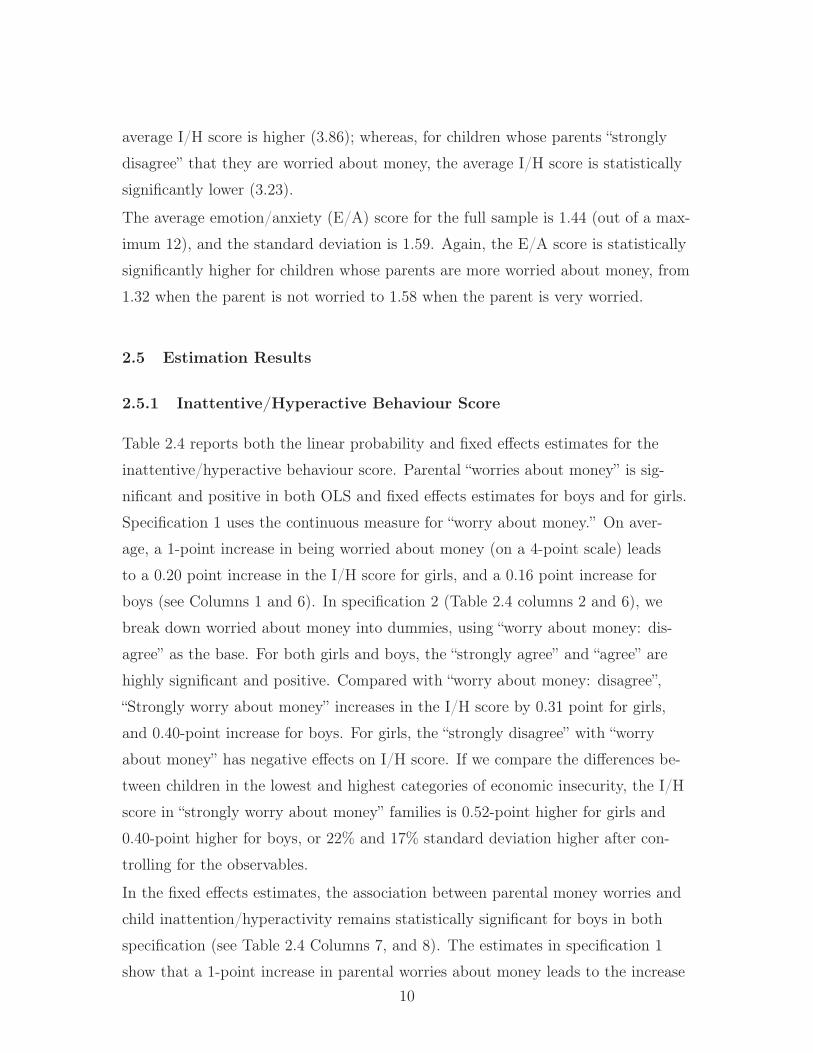
2.5 Estimation Results

2.5.1 Inattentive/Hyperactive Behaviour Score

Table 2.4 reports both the linear probability and fixed effects estimates for the

inattentive/hyperactive behaviour score. Parental “worries about money” is sig-

nificant and positive in both OLS and fixed effects estimates for boys and for girls.

Specification 1 uses the continuous measure for “worry about money.” On aver-

age, a 1-point increase in being worried about money (on a 4-point scale) leads

to a 0.20 point increase in the I/H score for girls, and a 0.16 point increase for

boys (see Columns 1 and 6). In specification 2 (Table 2.4 columns 2 and 6), we

break down worried about money into dummies, using “worry about money: dis-

agree” as the base. For both girls and boys, the “strongly agree” and “agree” are

highly significant and positive. Compared with “worry about money: disagree”,

“Strongly worry about money” increases in the I/H score by 0.31 point for girls,

and 0.40-point increase for boys. For girls, the “strongly disagree” with “worry

about money” has negative effects on I/H score. If we compare the differences be-

tween children in the lowest and highest categories of economic insecurity, the I/H

score in “strongly worry about money” families is 0.52-point higher for girls and

0.40-point higher for boys, or 22% and 17% standard deviation higher after con-

trolling for the observables.

In the fixed effects estimates, the association between parental money worries and

child inattention/hyperactivity remains statistically significant for boys in both

specification (see Table 2.4 Columns 7, and 8). The estimates in specification 1

show that a 1-point increase in parental worries about money leads to the increase10

in I/H score by 0.062 point for boys. The estimates in specification 2 demonstrates

that when parents strongly worry about money, the I/H score increases by 0.15

point compared with the same boy’s I/H score when parents do not worry about

money. The difference between highest and lowest categories suggest a 0.15-point

increase in I/H, which is an 8% standard deviation difference. This result suggests

that after controlling for unobserved heterogeneity across children, boys’ hyperac-

tivity increases with parental money worries, while girls’ I/H scores are not signifi-

cantly affected.

To better understand whether the magnitude of these effects is of potential policy

relevance, we compare the “worried about money” with “PMK has a college or uni-

versity degree” (relative to the base secondary education or less) in the OLS model

(see Table 2.4 Columns 1 and 5). A 1-point increase in being worried about money

(using the continuous measure) increases the inattentive/hyperactive behaviour

score by 0.20 for gilrs and 0.16 for boys, while PMK having a university education

decreases hyperactivity by 0.17. and 0.24 for boys. If we think that mother edu-

cation is a key correlate of child behaviour, this suggests that parental economic

insecurity has comparable effects in children: a 1-point increase in “worry about

money” on a 4-point scale could offset the effects of mother’s university education

in children’s upbringing.

2.5.2 Emotion/Anxiety Score

Table 2.5 reports both the OLS and fixed effects estimates for the emotion/ anx-

iety score. First, the continuous “worry about money” variable is significant and

positive for both genders (see Table 2.5 Columns 1 and 5). A 1-point increase in

parental economic insecurity is associated with a 0.14-point increase in anxiety

for girls, and a 0.08-point increase for boys, which is equivalent to a 9% of stan-

dard deviation increases for girls, and a 5% standard deviation increase for boys.

Specification 2 reports the estimates using categorical measures of worry about

money (see Columns 2 and 6). Comparing to “disagree with worry about money”,

“strongly worry about money” increases anxiety level by 0.19 point in girls and

0.23 point in boys, or 12% and 14% increase in standard deviation respectively.11

Each level of worry about money for girls are significant at a 1% level, with a neg-

ative effect associated with “Worry about money: strongly disagree” and a positive

effect associated with “Worry about money: strongly agree”. The difference in girls’

anxiety scores between the highest and lowest level of economic insecurity is 0.34

point (i.e. 21% standard deviation).

In the fixed effect estimations, “worry about money” is significantly associated with

a higher anxiety level for girls, though not for boys. For the continuous specifi-

cation, a 1-point increase in “worry about money” increases girls’ anxiety score

by 0.055 point on average. In the categorical specification, “strongly worry about

money” increases anxiety score by 0.15 point in girls, compare to the base “worry

about money: disagree”. It indicates a 10% standard deviation increase in girls’

anxiety score.1

Again, to put the magnitude of the economic insecurity estimate in context, we

compare it with the size of the divorce coefficient captured by the lone-parent vari-

able in the fixed effects model (see Table 2.5 Column 3 and 4). Compared to an

always-married family, a child whose parents divorce between the ages of 2/3 and

4/5 has an anxiety level that is 0.30 points higher. Changing from “Worry about

money: disagree” to “Worry about money: strongly agree” is associated with an

increase in the emotion/anxiety scale of 0.15 point. In other words, if economic in-

security changes from 2 to 4, the detrimental effect on girls’ anxiety is 50% of the

effect associated with divorce.2

1The fixed effects estimates show that income increases children’s anxiety score. It is possi-ble that income increases parents’ anticipation towards children which result in higher anxietyin children. It is also possible that the negative association with income is picking up the longerworking hours necessary for parents to earn higher incomes and one implication of greater work-ing time - parents spending less time with children. The latter hypothesis is supported by thenegative coefficient of income in the estimation of the positive interaction parenting score (seeSection 2.6).

2For both hyperactivity and anxiety scores, we test that the gender differences are significantby pooling boys and girls together and include gender interaction with “worry about money”.The estimates show that parental economic insecurity affects boys’ hyperactivity score more thangirls’, and girls’ anxiety score more than boys’.

12

2.6 Possible channels from parental economic insecurity to child

outcomes

From the previous section, we observe a negative relationship between children’s

non-cognitive skills and parental economic insecurity. The question subsequently

arises: why are children affected by parental economic insecurity? We propose that

two channels affect children: a direct channel and an indirect channel. The direct

channel is emotional mirroring, which is the subconscious imitation of another per-

son’s emotion (Chartrand & Bargh, 1999). Young children learn to behave and feel

by mimicry of the parents. If parents are tense, then children will mirror the tense-

ness. The indirect channel is through poor parenting behaviours associated with

economic stress. Exposure to stress hormones can change brain structure, affecting

cognition (Lupian et al, 2009). Parents under economic stress are more likely to

make poor parenting decisions.

Since the direct channel is not directly measurable, we examine parenting behaviours.

The NLSCY provides various parenting style indices designed by Dr. M. Boyle at

McMaster University and Dr. Ken Dodge at Vanderbilt University, including in-

effective parenting, irrational parenting, consistent parenting and positive interac-

tion. We use positive interaction and consistent parenting to represent “positive”

parenting behaviours, and we employ ineffective parenting and irrational parenting

to be proxies for “negative” parenting.

Each of the four parenting indicators is derived using a set of questions (detailed

question composition of the indices can be found in Appendix 1). The consistent

parenting style is constructed from questions about whether PMKs enforce rules,

and if the child can get out of punishment. A high score indicates more consistent

parenting. The positive interaction score is derived from questions such as if PMK

praises the child, laughs with them and plays games with the child. The ineffec-

tive parenting score uses questions about if PMKs have difficulty managing their

children, get annoyed and angry with their children. The irrational parenting style

score is from questions such as if the PMK yells at the child or uses physical pun-

ishment. High values of the first two parenting scores, and low values of the last

two parenting scores represent “positive” parenting.

To estimate the effects of economic insecurity on parenting styles, we substitute13

the dependent variables in Equations 2.1 ad 2.2 for the parenting indicators. Ta-

ble 2.6 reports the estimates of the association between parent reports of worry-

ing about money and the “positive” parenting index. The continuous measure of

“Worry about money” is significant and negative for both positive interaction score

and consistent parenting score in the OLS estimation, meaning economic insecu-

rity reduces the level of “positive” parenting. Specification 2 reports categorical

measure of “worry about money”. It shows that as parents are less worried about

money, they spend more times in positively interacting with their children and us-

ing more consistent parenting styles. The fixed effects estimation also indicates a

negative association between consistent parenting score for girls and parental eco-

nomic insecurity after controlling for the unobservables.

Table 2.7 shows the regressions for “negative” parenting style. The continuous mea-

sure of parental economic insecurity (1 to 4) is significant and positive in all OLS

and FE regressions indicating positive association between “worry about money”

and both the inefficient parenting score and irrational parenting scores”. In spec-

ification 2, “worry about money: strongly agree” is associated with high scores of

both inefficient parenting and irrational parenting. “Worry about money: strongly

disagree” is correlated with low scores of both negative parenting indicators. It

demonstrates that “negative” parenting strategies are more frequently adopted

when a higher level of economic insecurity is present (e.g., a parent may yell more

when stressed about money). If we compare the effects on “positive” with “nega-

tive” parenting indicators, parental economic insecurity increases “negative” parent-

ing more than it decreases “positive” parenting.

Those results strongly indicate that when parents worry about money, they spend

less time with their children, and are less able to enforce the rules. They are also

more likely to be angry with their children, and to use physical punishment. Thus,

we regard it as plausible that parental economic insecurity influences children at

least in part through parenting behaviours.14

2.7 Further results

One of the most important events that could affect children’s outcomes is divorce.

In the main estimation, we include both lone-parent families and married fami-

lies. There are three potential explanations: 1) Economic insecurity causes family

dissolution and thus affecting child outcomes; 2) Family dissolution affects both

economic insecurity and child outcomes; 3) Economic insecurity directly affects

child outcomes. Therefore, to remove the confounding effects from divorce, we re-

estimate Equations 2.1 and 2.2 in two samples: 1) children in lone-parent families

(14% of the full sample) and 2) children whose parents are always married (84% of

the original sample).

Table 2.8 shows the estimates of hyperactivity and anxiety using lone-parent only.

The estimates indicate that economic insecurity remains statistically significant for

girls in the OLS estimation, but not in the fixed effects estimation. The effects on

boys’ hyperactivity becomes insignificant for lone-parent families. “Worry about

money” measures are significant on emotional disorder/anxiety scores, especially

in fixed effects estimation for girls and the OLS estimation for boys. The anxiety

score increases more significantly with “worry about money” for both continuous

measure and the categorical measure than the full sample estimates.

Table 2.9 shows the estimates of hyperactivity and anxiety scores using always-

married families only. Compared to the full sample estimation, girls’ hyperactivity

estimates are similar to the full sample estimation, while boys’ hyperactivity esti-

mates are more significant than the full sample estimation. The anxiety scores for

both genders are not significantly different from the full sample estimation.

The results indicate that girls in lone-parent families are more likely to be anx-

ious, and boys in always-married families are more likely to be hyperactive than

the population average. It means that without the changes in parents’ marital sta-

tus, the economic insecurity still increases girls’ anxiety and boys’ hyperactivity.

Thus, it is plausible to draw the conclusion that parental economic insecurity hin-

ders the development of children’s non-cognitive skills.15

2.8 Conclusion

This paper studies connections between parental economic insecurity and outcomes

for 2 to 5 year-old Canadian children. Results for both OLS and fixed effects mod-

els suggest that inattentive/hyperactive behaviours and emotional/anxious be-

haviours are positively associated with parents being ’worried about having enough

money to meet family needs.’ We illustrate that a plausible channel from parental

economic insecurity to children’s outcomes is through the parenting behaviours.

Less “positive” and more “negative” parenting strategies are reported when parents

experience economic insecurity.

Future research can focus on attempting to quantify the “direct” and “indirect”

channel of parental economic insecurity on children. A cross-country comparison

between the United States and Canada using National Longitudinal Survey of

Youth may allow for more variation in policy, which may improve/worsen economic

security for parents.

16

Table 2.1: Distribution of “You worry about whether the money you have will beenough to support your family?” Answered by PMKs of girls and boys at age 2 to5. Year 2000 to 2008.

Worry about money Distribution

Strongly disagree 0.17Disagree 0.36Agree 0.33Strongly agree 0.15

Total 1Source: NLSCY, pooled cross-sections.

17

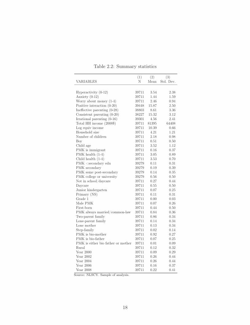
Table 2.2: Summary statistics

(1) (2) (3)VARIABLES N Mean Std. Dev.

Hyperactivity (0-12) 39711 3.54 2.38Anxiety (0-12) 39711 1.44 1.59Worry about money (1-4) 39711 2.46 0.94Positive interaction (0-20) 39448 15.87 2.50Ineffective parenting (0-28) 38803 8.61 3.36Consistent parenting (0-20) 38227 15.32 3.12Irrational parenting (0-16) 39301 4.56 2.41Total HH income (2008$) 39711 81395 64408Log equiv income 39711 10.39 0.66Household size 39711 4.21 1.21Number of children 39711 2.18 0.98Boy 39711 0.51 0.50Child age 39711 3.52 1.12PMK is immigrant 39711 0.16 0.37PMK health (1-4) 39711 3.05 0.89Child health (1-4) 39711 3.53 0.70PMK <secondary edu 39279 0.11 0.31PMK secondary 39279 0.19 0.39PMK some post-secondary 39279 0.14 0.35PMK college or university 39279 0.56 0.50Not in school/daycare 39711 0.27 0.44Daycare 39711 0.55 0.50Junior kindergarten 39711 0.07 0.25Primary (NS) 39711 0.11 0.31Grade 1 39711 0.00 0.03Male PMK 39711 0.07 0.26First-born 39711 0.44 0.50PMK always married/common-law 39711 0.84 0.36Two-parent family 39711 0.86 0.34Lone-parent family 39711 0.14 0.34Lone mother 39711 0.13 0.34Step-family 39711 0.02 0.14PMK is bio-mother 39711 0.92 0.27PMK is bio-father 39711 0.07 0.25PMK is either bio father or mother 39711 0.01 0.09Rural 39711 0.12 0.32Year 2000 39711 0.09 0.29Year 2002 39711 0.26 0.44Year 2004 39711 0.26 0.44Year 2006 39711 0.16 0.37Year 2008 39711 0.22 0.41

Source: NLSCY. Sample of analysis.

18

Table 2.3: Mean inattention/hyperactivity and emotion/anxiety scores for 2 to 5year-old Canadian children, by level of parental economic insecurity, year 2000 to2008.

Outcome Hyperactivity AnxietyMean Std. Err [95% Conf. Interval] Mean Std. Err [95% Conf. Interval]

Not at all worry about money 3.23 0.05 3.13 3.33 1.32 0.03 1.26 1.38Not worry about money 3.39 0.03 3.33 3.46 1.36 0.02 1.32 1.41Worry about money 3.70 0.04 3.63 3.78 1.52 0.03 1.47 1.57Strongly worry about money 3.86 0.05 3.75 3.96 1.58 0.04 1.50 1.65

Source: NLSCY

Table 2.4: OLS and fixed effect estimates of inattentive/hyperactivity score. Chil-dren from age 2 to 5. Year 2000 to 2008.

Girl Boy(1) (2) (3) (4) (5) (6) (7) (8)

VARIABLES OLS OLS FE FE OLS OLS FE FE

Worry about money (1-4) 0.201*** 0.0450 0.160*** 0.0623*(0.0335) (0.0317) (0.0346) (0.0326)

Worry about money=4 0.308*** 0.102 0.396*** 0.153*(0.0929) (0.0833) (0.0928) (0.0858)


Worry about money=1 -0.210*** -0.0163 -0.0163 0.00275(0.0791) (0.0699) (0.0889) (0.0709)

PMK has a college or university degree -0.166** -0.162** -0.241*** -0.242***(0.0656) (0.0653) (0.0682) (0.0681)

Observations 19,200 19,200 19,408 19,408 20,079 20,079 20,303 20,303R-squared 0.054 0.055 0.005 0.005 0.049 0.050 0.003 0.003Time-variant controls Yes Yes Yes Yes Yes Yes Yes YesTime-invariant controls Yes Yes No No Yes Yes No NoNumber of persruk 13,245 13,245 13,923 13,923

Source: NLSCY. Standard errors clustered at the household level. *** p<0.01, ** p<0.05, * p<0.1.

Note: “Worry about money=1” indicates “Worry about money: strongly disagree”, and “Worry about money=4’

indicates “Worry about money: strongly agree”. Time-variant controls include log equivalent income, child’s health,

PMK’s health, lone-parent, and step-family. Time-invariant controls include child age, first-born, child schooling,

number of children, PMK and child relationship, PMK’s health, PMK is an immigrant, PMK’s education, rural,

province of residence and survey year.

19

Table 2.5: OLS and fixed effect estimates of emotion/anxiety score. Children fromage 2 to 5. Year 2000 to 2008.

Girl Boy(1) (2) (3) (4) (5) (6) (7) (8)

VARIABLES OLS OLS FE FE OLS OLS FE FE

Worry about money (1-4) 0.138*** 0.0554** 0.0804*** -0.00411(0.0236) (0.0230) (0.0221) (0.0237)

Worry about money=4 0.193*** 0.153** 0.232*** -0.0544(0.0667) (0.0629) (0.0632) (0.0614)

Worry about money=3 0.231*** 0.0595 0.105** 0.0460(0.0519) (0.0440) (0.0447) (0.0429)

Worry about money=1 -0.148*** -0.0124 0.00828 -0.0112(0.0517) (0.0498) (0.0548) (0.0537)

Lone-parent family 0.0226 0.0373 0.298*** 0.297*** 0.0800 0.0709 0.422*** 0.430***(0.0781) (0.0779) (0.111) (0.111) (0.0718) (0.0722) (0.110) (0.110)








20

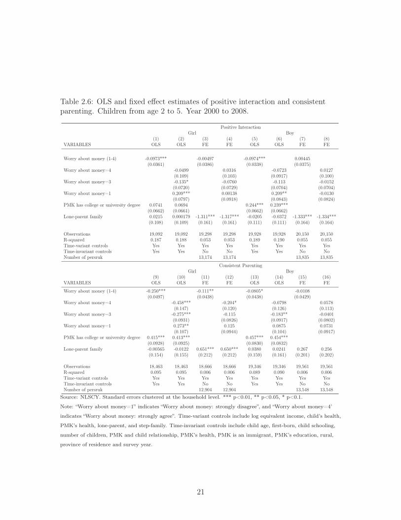
Table 2.6: OLS and fixed effect estimates of positive interaction and consistentparenting. Children from age 2 to 5. Year 2000 to 2008.

Positive InteractionGirl Boy

(1) (2) (3) (4) (5) (6) (7) (8)VARIABLES OLS OLS FE FE OLS OLS FE FE

Worry about money (1-4) -0.0973*** -0.00497 -0.0974*** 0.00445(0.0361) (0.0386) (0.0338) (0.0375)

Worry about money=4 -0.0499 0.0316 -0.0723 0.0127(0.109) (0.103) (0.0917) (0.100)

Worry about money=3 -0.135* -0.0760 -0.113 -0.0152(0.0720) (0.0729) (0.0704) (0.0704)

Worry about money=1 0.209*** 0.00138 0.209** -0.0130(0.0797) (0.0918) (0.0843) (0.0824)

PMK has college or university degree 0.0741 0.0694 0.244*** 0.239***(0.0662) (0.0661) (0.0662) (0.0662)

Lone-parent family 0.0215 0.000179 -1.311*** -1.317*** -0.0205 -0.0372 -1.333*** -1.334***(0.108) (0.109) (0.161) (0.161) (0.111) (0.111) (0.164) (0.164)


Consistent ParentingGirl Boy


Worry about money (1-4) -0.250*** -0.111** -0.0805* -0.0108(0.0497) (0.0438) (0.0438) (0.0429)

Worry about money=4 -0.458*** -0.204* -0.0798 0.0578(0.147) (0.120) (0.126) (0.113)

Worry about money=3 -0.275*** -0.115 -0.183** -0.0401(0.0931) (0.0826) (0.0917) (0.0802)

Worry about money=1 0.273** 0.125 0.0875 0.0731(0.107) (0.0944) (0.104) (0.0917)

PMK has college or university degree 0.415*** 0.413*** 0.457*** 0.454***(0.0928) (0.0925) (0.0830) (0.0832)

Lone-parent family -0.00565 -0.0122 0.651*** 0.650*** 0.0380 0.0241 0.267 0.256(0.154) (0.155) (0.212) (0.212) (0.159) (0.161) (0.201) (0.202)








21

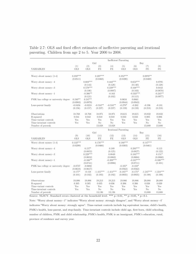
Table 2.7: OLS and fixed effect estimates of ineffective parenting and irrationalparenting. Children from age 2 to 5. Year 2000 to 2008.

Inefficient ParentingGirl Boy


Worry about money (1-4) 0.359*** 0.207*** 0.352*** 0.0970**(0.0511) (0.0468) (0.0490) (0.0469)

Worry about money=4 0.603*** 0.444*** 0.653*** 0.0795(0.144) (0.128) (0.140) (0.128)

Worry about money=3 0.579*** 0.229*** 0.448*** 0.0443(0.106) (0.0887) (0.103) (0.0870)

Worry about money=1 -0.306** -0.163 -0.333*** -0.245**(0.121) (0.102) (0.115) (0.0977)

PMK has college or university degree 0.240** 0.247** 0.0634 0.0661(0.0983) (0.0979) (0.0944) (0.0943)

Lone-parent family -0.0456 -0.0218 -0.534** -0.534** -0.270* -0.262 -0.196 -0.181(0.156) (0.157) (0.237) (0.237) (0.159) (0.159) (0.218) (0.218)


Irrational ParentingGirl Boy


Worry about money (1-4) 0.133*** 0.176*** 0.180*** 0.147***(0.0299) (0.0466) (0.0303) (0.0461)

Worry about money=4 0.157* 0.189 0.293*** 0.113(0.0852) (0.125) (0.0827) (0.122)


Worry about money=1 -0.166** -0.389*** -0.247*** -0.326***(0.0741) (0.0986) (0.0711) (0.101)

PMK has college or university degree -0.0737 -0.0692 -0.105* -0.103*(0.0618) (0.0617) (0.0562) (0.0562)

Lone-parent family -0.177* -0.158 -1.415*** -1.414*** -0.185** -0.175* -1.247*** -1.224***(0.101) (0.102) (0.193) (0.192) (0.0935) (0.0935) (0.198) (0.198)








22

Table 2.8: OLS and fixed effect estimates of hyperactivity and anxiety scores.Children from age 2 to 5 in lone-parent families. Year 2000 to 2008.

HyperactivityGirl Boy


Worry about money (1-4) 0.221*** 0.0588 0.0994 0.117(0.0829) (0.0938) (0.0982) (0.102)

Worry about money=4 0.392* 0.126 0.263 0.217(0.208) (0.220) (0.215) (0.243)

Worry about money=3 0.256 0.138 0.0395 0.0862(0.201) (0.202) (0.202) (0.211)

Worry about money=1 -0.335 -0.0450 0.0569 -0.162(0.314) (0.331) (0.355) (0.358)


AnxietyGirl Boy


Worry about money (1-4) 0.1000* 0.150** 0.139** -0.0513(0.0580) (0.0622) (0.0625) (0.0891)

Worry about money=4 0.0784 0.280* 0.285** -0.105(0.152) (0.151) (0.134) (0.192)

Worry about money=3 0.150 0.0791 0.157 0.0353(0.126) (0.142) (0.117) (0.167)

Worry about money=1 -0.390** -0.192 -0.116 0.0298(0.175) (0.202) (0.221) (0.289)








23

Table 2.9: OLS and fixed effect estimates of hyperactivity and anxiety scores.Children from age 2 to 5 with married parents. Year 2000 to 2008.

HyperactivityGirl Boy


Worry about money (1-4) 0.211*** 0.0492 0.163*** 0.0503(0.0364) (0.0350) (0.0375) (0.0356)


Worry about money=3 0.337*** 0.0635 0.275*** 0.0864(0.0762) (0.0669) (0.0797) (0.0663)

Worry about money=1 -0.206** -0.00243 0.00584 0.0348(0.0813) (0.0738) (0.0928) (0.0729)


AnxietyGirl Boy


Worry about money (1-4) 0.140*** 0.0490* 0.0755*** -0.00276(0.0255) (0.0253) (0.0237) (0.0250)

Worry about money=4 0.195*** 0.161** 0.243*** -0.0611(0.0745) (0.0724) (0.0718) (0.0684)

Worry about money=3 0.243*** 0.0590 0.0974** 0.0296(0.0561) (0.0483) (0.0486) (0.0454)

Worry about money=1 -0.127** 0.00896 0.0205 -0.0215(0.0537) (0.0525) (0.0568) (0.0553)








24

Chapter 3

Fatter Kids and the Shattered “Iron Rice Bowl”:

Intergenerational Effects of Economic Insecurity During

Chinese State-Owned Enterprise Reform

3.1 Introduction

Economic insecurity, or the perception of “a significant and unavoidable downside

economic risk” in the future (Osberg, 1998 and 2015a), is an expectation of future

economic losses which results from past and present experiences. It is not only a

leading cause of family dissolution (Larson et al., 1994), but also contributes to

deterioration of health (Tsutsumi et al., 2001; Rohde et al., 2016; Watson, Osberg

& Phipps, 2016; Rohde, Tang & Osberg, 2017).

Blanchflower and Oswald (1999), Clark and Grey (1997), Hacker et al. (2010)

have argued that economic insecurity has been on a gradual rise since the 1970s in

countries all around the world, but in few cases has economic insecurity surged as

dramatically and influentially as in China during the late 1990s. Because of state-

owned enterprise (SOE) reform, 34 million workers from the state sector were laid

off between 1995 and 2001, thereby heightening the insecurity of the 51 million

continuing SOE employees. The magnitude and speed of these changes occurred at

historically unprecedented rates.

Layoffs from state-owned enterprise reform were particularly harsh on state sector

workers because: (1) the state sector in China had never witnessed employment

uncertainty before this layoff policy, making the workers especially unprepared.

Therefore, the job losses were unanticipated and involuntary; (2) the social safety

net was under-developed in China. Little social assistance or job-search assistance

was provided to the laid-off workers; (3) laid-off workers were mostly older, un-

skilled, and female, which added to the challenges of re-employment. These disad-

vantages made the economic insecurity to which they were subjected particularly

25

significant.

One of the most common outcomes for health is body mass indicator (BMI). Among

other causes, it has been well-established that greater economic insecurity increases

weight gain in adults (Smith 2009; Watson et al., 2016; and Rohde et al., 2016).

The innovation of this study is to examine the intergenerational effects of such

insecurity and the effects of greater parental economic insecurity in a developing

country (China) on children and adolescents.

Cole et.al. (2000) document that the prevalence of obesity has increased dramat-

ically in developed countries. In developing countries, malnutrition and infectious

diseases are declining, while obesity, cardiovascular diseases, and Type 2 diabetes

are rising (WHO, 2000). In 2011, 30% of Chinese adults and 11% of Chinese chil-

dren were overweight (Yan et al., 2012).

Child obesity not only leads to adult obesity (Abraham et al., 1971; Guo et al.,

1994; Sorensen & Sonne-Holm, 1988) but also chronic diseases, such as impaired

glucose metabolism, hypertension, coronary arteries (Kavey, et al., 2003). Child

obesity is particularly linked to the development of Type 2 diabetes at a younger

age (WHO 2000) and can also adversely influence psychological wellbeing later in

life (Friedman and Brownell, 1995)

To account for rates of maturation and growth, I use the most prominent refer-

ences including the World Health Organization (WHO) growth standard, and the

United States Centers for Disease Control and Prevention (CDC) standards to

adjust BMI and weight for age and gender specific measures. I also include the

waist-to-height ratio to complement BMI measures following suggestions in the

medical literature (Mokha et al., 2010; Schneider et al., 2010; Yan et al. 2007;

and Burkhauser & Cawley, 2008). The waist-to-height ratio distinguishes body

fat from bones and muscles, and differentiates abdominal fat from skin fat. Yan

et al. (2007) note the racial neutrality of the waist-to-height ratio and that it is an

accurate measure for Chinese children.

I estimate the effects on the BMI measures and waist-to-height ratio using the ex-

pected economic loss at Chinese provincial- and year-levels (i.e., treatment with

different intensities). A continuous difference-in-difference model compares the lay-

off effects in the state sector (treatment group by changes in layoff policy) and the26

non-state sector (control group, not directly affected by changes in the state sector

layoff policy). The results show a significantly greater weight gain in boys whose

parents work in the state sector when the expected economic loss is high. The re-

sults persist for boys of parents working in the state sector even if neither parent

actually experienced a layoff. It suggests that anxiety about the future (i.e., eco-

nomic insecurity) is at least a major reason for weight gain in children. I examine

the differential impacts of economic insecurity – the probability of job loss and fi-

nancial loss of layoff. The probability of job loss has more significant negative ef-

fects on child weight gain than the severity of financial loss of layoff.

The non-constant effects of parental economic insecurity on children’s weight gains

are examined using quantile regressions. The rational is to test if parental insecu-

rity has larger impacts on children’s weight gain for those who are already over-

weight, versus making children who are underweight and become normal weight.

The results suggest more severe effects of weight gain in heavier children caused by

parental economic insecurity. This means the threat posed by weight gain in chil-

dren is greater because the weight gain is more significant in children above normal

weight.

3.2 China State-Owned Enterprise Reform

During Mao Zedong’s era, China was a planned economy. Jobs were assigned ac-

cording to quotas decided by government and job candidates had little freedom to

choose their employment. Lifelong employment of urban workers was provided by

the government with benefits that include child care, health care, housing and pen-

sions (Lee, 2000). State sector employment, therefore, was considered an “iron rice

bowl”, with no economic insecurity.

Inefficiency in resource allocation and the lack of work incentives shattered the

“iron rice bowl” (Lin, Cai & Li, 1998). In 1995, China enacted a new labour law

that allowed the dismissal of no-fault workers. A new word, Xia Gang (Layoff),

was thus invoked and used in the China Labour Statistics Yearbook. In 1997, lay-

offs were further intensified by extending the new labour law to large-scale state-

owned enterprises. From 1995 to 2001, state-owned sector employment dropped

from 113 million to 67 million, a 40% decrease. According to the China Urban27

Labour Survey, these layoffs caused the unemployment rate to surge to more than

10%, and labour force participation to decline by up to 8.9% in representative

cities. The state-owned enterprise reform introduced employment uncertainty for

the first time since the establishment of the Communist Government in 1949 (Giles,

Park & Cai, 2006).

3.2.1 Social support

Living subsidies for laid-off workers were initially provided by the original employ-

ers (i.e., the state-owned enterprises). In the late 1990s, protection against job loss

gradually shifted to unemployment insurance. In general, social insurance pro-

grams in China in the late 1990s were severely underdeveloped; hence provided

little protection against unexpected job loss. Unemployment insurance (UI) system

was introduced in China in 1986. Benefit levels were set by the local government

at a range between minimum living standards (Dibao) and the minimum wage

rate. Compared to developed countries, UI in China provides a much lower income

replacement rate. For example, in 2005, the UI benefits paid as a percentage of av-

erage urban on-work wages was only 14.7% (Giles, Park & Cai, 2006).

The duration of benefits depends on the UI contributions, and may last up to 24

months. To qualify for UI, workers must meet the following conditions: 1) have

contributed to UI for at least a year; 2) are terminated involuntarily, 3) are willing

to work. By the early 2000s, it only covered 40% of urban workers (Giles, Park

& Cai, 2006). With the low coverage and low replacement rate, laid-off workers

had to rely on personal savings and private support from relatives. The structural

change in the economy increased the difficulties for laid-off workers to find new

jobs without the support of adequate job training program. The re-employment

rate of the laid-off workers from the state sector was only 29.1% after one year,

and 36.9% after five years (Giles, Park & Cai, 2006).

The remaining state employees were also affected by the reform, experiencing wage

and pension arrears and benefits reductions including decreased health insurance

coverage and housing benefits. These on-job economic losses along with the now

greater potential for outright job loss meant a significant increase in anxiety and

economic insecurity for continuing state workers. In other words, the impact of the28

new layoff policy was not limited to those actually laid-off in the state sector.

3.3 Mechanism of Health Effects of Economic Insecurity

3.3.1 Overeating and Economic Insecurity

The causal relationship between adult weight gain and economic insecurity has

recently been established in economic literature. Offer et al. (2010) use macro-

level data from 11 developed countries over ten years and suggest the obesity epi-

demic is mainly contributed by social insecurity. Where socioeconomic supports

do not provide much protection against economic losses, people tend to respond

more to fast food “shock” because of the economic stress. When the possibility of

economic loss is well-insured by social programs, even though there is abundant

calorie rich food, people tend to not overeat and obesity prevalence is significantly

lower. Smith, Stoddard and Barnes (2009) use 12 years panel data from the United

States National Longitudinal Survey of Youth, and find that a one-percentage-

point rise in the probability of becoming unemployed increases adult weight gain

by 0.6 pounds, and the social safety net decreases the negative effect of economic

insecurity. Using the Canadian Community Health Survey data, Watson, Osberg

and Phipps (2016) exploit the unemployment insurance benefit cuts in the 1990s as

an exogenous “natural experiment” variation in economic insecurity, and establish

the causal relationship between economic insecurity and the BMI gain in adults.

Rohde, Tang and Osberg (2017) use the Household, Income and Labour Dynam-

ics in Australia (HILDA) Survey and find that the economic insecurity and adult

obesity form a self-sustaining vicious cycle.

Literature in psychology and neuroscience has linked stress to overeating (Greeno

and Wing, 1994). Stress induces people to turn to “comfort food” that is high in

calorie and fat (Dallman et al., 2003). Smith (2009) suggests there is a biochem-

ical mechanism of stress which can cause overeating. Like other animals, humans

compensate for food uncertainty by overeating and storing body fat. The ability

to store body fat is a survival instinct when the risk of starvation is present, and

over-eating has been genetically “hard-wired” as a response to anxiety about future

food availability. Although the risk of starvation is minimal for most contemporary29

humans in affluent societies, stress and anxiety still come from economic uncer-

tainties. In the presence of economic hazards, genes influence human behaviour

and humans respond by overeating as a form of “self-medication” for stress—as the

phrase “comfort foods” might suggest. In the Chinese context, it is worth noting

that parents in the state sector have higher income than those in the non-state sec-

tor (see Table 3.3. Therefore, parents are economically able to purchase calorie rich

food.

The innovation of this study is the intergenerational transmission mechanism. The

possible channels include, inter alia: 1) economic insecurity increases precaution-

ary savings of the family, thus reducing the monetary investment in the child. 2)

Future uncertainty increases parents work hours to compensate for potential eco-

nomic losses, thus reducing the time investment of the child and the positive inter-

action with the child. 3) Eating healthy takes time and energy. Economic insecu-

rity generates mental stress for the parents. If a parent is stressed and make poor

nutritious choices, it is difficult for the parent to deny the child from accessing the

“junk food”. 4) Under economic stress, parents are less likely to be able to enforce

rules that keep their children eating healthy food. Other irrational parenting deci-

sions may also occur as a result of economic anxiety.

3.3.2 Theoretical framework of intergenerational economic insecurity

I use three measures of economic insecurity: the probability of job loss, the finan-

cial loss from job loss, and expected economic loss from the fear of job loss. The

three measures are defined as follow:

Prob(Layoff) = P (3.1)

E(FinancialLoss) = E[ΔY |Layoff ] = Δ (3.2)

E(EconomicLoss) = Prob(Layoff) · E(FinancialLoss) = P ·Δ (3.3)

The economic insecurity at time t is based on the current and past experience:

Insecurityt = f(Pt−1Δt−1, PtΔt) (3.4)30

Heckman (2007) outlines how parental investment affects children’s capabilities.

These parental effects on children have focused mostly on positive investments,

such as nutrition and care. In this chapter, I include the negative impact of parental

economic insecurity on children’s human capital formation, using Heckman (2007)’s

model as the guideline. A child’s capability production, θ at time t+1, is deter-

mined by the following factors: an initial endowment, θ0 (e.g., genetic condition);

parents’ capabilities (e.g., parents’ IQ, income, and education), h; parents’ invest-

ment at period t, It. The level of investment is then determined by the economic

insecurity at time t, Insecurityt. The simplified production function for three peri-

ods of human capital formation is

θt+1 = f(h, θ0, It(Insecurityt|Pt−1Δt−1, PtΔt) (3.5)

where ∂θt+1

∂It> 0 ,and ∂It

∂Insecurityt< 0. The first condition suggests that greater in-

vestment from parents promotes higher human capital formation of the child. The

second condition assumes that a high degree of economic insecurity is associated

with a low investment.

Three groups experience different changes in economic insecurity PtΔt. Group 1

is identified as the non-state sector, experiencing no change in expected layoff and

financial loss from layoff, thus δInsecurity = 0 . Group 2 can be the state sector in

mildly affected province, where there is low expected economic loss, δInsecurity =

low. Group 3 represents the state sector in the province that is affected severely by

the layoff policy, and high economic loss is expected, δInsecurity = high .

The effect of parental economic insecurity on a child’s outcome is denoted by α1 =

∂θ∂Insecurity

. The differential effect of the probability of job loss is captured by β1 =∂θt+1

∂P, and the severity of financial loss from layoff is β2 = ∂θt+1

∂δ. The empirical

strategy to estimate α1, β1, and β2 is explored in section 6.

3.4 Data

3.4.1 China Health and Nutrition Survey

This chapter uses data from the China Nutrition and Health Survey (CHNS) con-

ducted by the University of North Carolina, Chapel Hill and the Chinese Center31

for Disease Control and Prevention (CCDC). The CHNS is the only large-scale

longitudinal household level survey in China (Popkin et al., 2010); it consists of

9 panels from 1989 to 2011 of more than 4000 households and 15,000 individu-

als. The data are collected at the community, household, and individual levels,

and includes detailed information on economic, health, sociological, and demo-

graphic circumstances. Households are selected in both rural and urban areas in

eight provinces: Liaoning, Shandong, Henan, Jiangsu, Hubei, Hunan, Guizhou, and

Guangxi with multistage, random cluster design, stratified by income.

All household members are interviewed during the survey, and children younger

than 10-years-old are assisted by their parents. One to six children in one family

can be observed in the sample. On average, there are two children per family in

the CHNS sample1. Special efforts are made to interview during the early morning

or on weekends to avoid missing children who attend boarding school or migrant

workers. The attrition rate at the household level is 10% from the previous cycle,

and 31% from 1989 to 2006 (Popkin et al., 2010). Anthropometric measures, such

as height and weight, are taken on site by the CHNS interviewers who had seven

days of training by the collaborating teams. Children are measured without shoes

and with light clothes to the nearest 0.1 cm and 0.1 kg respectively during the in-

terview (Yan et al., 2012).

The CHNS has several features that make it particularly suitable for the study.

First, the longitudinal structure provides a comparison of the outcomes of the

same child before, during and after the state-owned enterprise reform period. Sec-

ond, the large sample size enables analysis based on provincial heterogeneity as

well as differences between state and non-state enterprises. Third, the CHNS has

data not only on a single household member, but also on parents, spouses, and

children based on the person-specific interviews, making it ideal for examining

the spill-over effects of economic insecurity. Fourth, the CHNS interview questions

cover not only labour market outcomes, such as employment status, sectors, and

earnings of both parents, but also the health outcomes of the child, and other de-

mographic characteristics of the family. The extensive and in-depth information

enables the inclusion of almost all control variables used in the related literature.

1The one child policy does not generally apply in rural areas (Hesketh, Lu & Xing, 2005).

32

A supplementary dataset on layoffs is also used and comes from China Labour

Statistics Yearbook produced by the National Bureau of Statistics of China. It

reports the number of laid-off workers at year-end as well as the number of state-

sector employees at the year-end by province from 1995 to 2005. These two vari-

ables allow estimates of the layoff rate across provinces and over time. It also re-

ports the off-post (laid-off) state sector workers’ living subsidies and the on-post

(on the job) state-owned enterprise workers’ average wage by province; from this

the financial loss from layoff can be calculated.

3.4.2 Longitudinal Sample

The sample for this study is children and adolescents 4 to 18 years-old in every

cycle who entered the survey in 1989, 1991 and 1993 (pre-reform cycles). The birth

cohort of the sample is 1979 to 1993 and is observed in 1997, 2000, and 2004. There

are 1,730 children and adolescents in the longitudinal sample and 2,636 observa-

tions in the pooled cross-sectional sample. Table 3.1 shows the number of same

children observed in the panel in each year. Table 3.2 presents the age and year

structure of the sample. Attrition comes mainly from the age limit of 18 years.

Only “always married couples” are included for two reasons. First, the divorce

rate during the survey period is extremely low (2%). Second, household disso-

lution itself can cause enormous mental and financial stress on family members,

which would confound the estimated effects being examined. I also exclude fam-

ilies with negative income. The CHNS noted many households with negative net

income from their business, especially those raising livestock. The nature of such

businesses involves substantial initial investment, and the return may take years to

happen. Therefore, the negative income does not necessarily reflect the economic

condition of the family. Mothers who are above 60 years old and fathers above 70

years old are excluded from the sample (2 observations).

3.4.3 Definitions of Weight Measures

In this study, the two prominent international references for children’s BMI mea-

sures are used. The first outcome variable in the study is the body mass index33

(BMI) Z-score using the World Health Organization (WHO) child growth stan-

dards for 0 to 5 year-olds (World Health Organization, 2006) and WHO growth

reference for 5 to 19 year-olds (Onis et al., 2007). The WHO growth standards col-

lect data for healthy infants and young children from Brazil, Ghana, India, Nor-

way, Oman and the United States, and the WHO growth references use the Na-

tional Center for Health Statistics (NCHS) data, merged with a growth standard

cross-sectional sample. Using the Box-Cox-power-exponential (BCPE) method and

LMS methods (Cole and Green, 1992), the WHO constructs BMI for age, adjust-

ing for skewness and kurtosis (see Figure 2 for growth charts). The BMI Z-score is

calculated using the following equation.

BMIZit =BMIit − ¯BMIWHO

σBMIWHO

(3.6)

where for child i in year t. The BMI Z-score measures how many standard de-

viations the child’s BMI is from the gender and age specific median defined by

WHO standards. Different from a unified BMI cutoff for all adults, the standard

of BMI varies according to children’s age and gender. According to the WHO stan-

dard, the median BMI is 15.2 for 5-year-old girls and 21.7 for 18-year-old-boys. By

adopting the BMI Z-score, the outcome variable reflects the different standards at

each growth stage of children. Observations that are over 5 standard deviations

from the median are excluded in the sample according to WHO recommended out-

lier cutoffs.

The second variable is a weight-for-age Z-score using the United States Centers

Disease Control 2000 Growth Reference with LMS method (Kuczmarski et al.

2000). The weight-for-age Z-score is generated in a similar manner to the BMI Z-

score. It measures how many standard deviations the child’s weight (in kg) is from

the median of the age and gender specific group:

WFAZit =Weightit − ¯WeightCDC

σWeightCDC

(3.7)

The mean of weight-for-age Z-score in the CHNS sample is -1.11. The state sector

is -0.67, while the non-state sector is -1.18. The difference between the two sectors

suggests that the state sector is the “better-off” group in the sample. Therefore,34

weight gains in the state sector are less likely to imply children with malnutrition

moving out of their underweight classification. Rather it suggests gaining weight

by already well-fed children.

The first two outcome variables capture the different perspectives of weight gain

with the leading international standards. Although BMI-related measures are fre-

quently used in estimating the risk of obesity on morbidity risks, it has some ma-

jor limitations. First, they do not distinguish fat from non-fat mass, such as mus-

cle and bones, which would mistakenly classify an athlete with large muscle mass

in the overweight category. Second, they do not inform the fat distribution in the

body: If the fat is distributed in the abdominal area (i.e., if it is visceral fat) rather

than underneath the skin (i.e., if it is subcutaneous fat), then it links to elevated

cardiovascular risks (Schneider et al., 2010; Kuczmarski et al., 2000). Third, they

are not specifically generated according to the Chinese population, nor are they

adjusted for the recent trend of increase in child obesity. Negative health effects of

obesity are found in the Asian population with a lower BMI (World Health Orga-

nization, 2000). Studies suggest that morbidity increases when BMI is greater than

23 in an Asian population (Ko et al., 1999; Deurenberg et al., 2002) instead of the

cut-off of 25 used in adult Europids.

A growing medical literature (Mokha et al., 2010; Schneider et al., 2010; Yan et al.

2007; and Burkhauser & Cawley, 2008) argues that abdominal obesity is a more

accurate indicator of health risks than BMI, and the waist-to-height ratio provides

an accurate measure of evaluating child and adolescent obesity. In the normal

weight group, children with central obesity (high waist circumference) are more

likely to have adverse levels of LDL cholesterol, HDL cholesterol, triglycerides, and

insulin; while children in overweight and obese groups without central obesity are

less likely to have morbidity risks such as Type 2 diabetes mellitus, hypertension

or metabolic syndrome than those with central obesity (Mokha et al., 2010)

To complement the other measures, I use waist-to-height ratio (WHtR) as the

third outcome variable. It is defined as waist circumference divided by height,

measured in the same unit. The advantages of the waist-to-height measure in-

clude its wide availability, accuracy and non-age- and race-dependency (Yan, 2007;

Mokha, 2010). It not only provides information on body fat and fat distribution,35

but also is comparable as it is age, gender, and race neutral. The kernel density

distributions of the three outcome variables are presented in Figure 3. The distri-

butions show a positive skewness, which corresponds to the previous literature that

lower mean in the BMI is associated with Asian population (World Health Organi-

zation, 2000).

3.4.4 Economic insecurity and exogeneity of layoff policy

“Individuals feel economically insecure when they perceive a significant downside

economic risk, which they are unable to adequately insure against or avoid or ig-

nore” (Osberg, 1998 & 2015). In this study, change in expected economic loss in

the state sector is the reason for greater economic insecurity, which can be thought

about in three ways: first, the possibility of being laid off (layoff rate), where

LayoffRatept =Number of laid-off workers in state sectorpt

Number of state sector workerspt(3.8)

i.e., the layoff rate is measured by the number of laid off workers divided by the

total number of state sector workers in the province p and year t; second, the fi-

nancial loss if laid off:

FinancialLosspt = 1− Average living subsidies of laid-off workersptAverage wage rate of on-the-job workers in state sectorpt

(3.9)

i.e., the average percentage income drop for laid-off workers in province p and year

t; and third, the expected economic loss:

E(EconomicLoss)pt = LayoffRatept · FinancialLosspt (3.10)

i.e., the product of probability of layoff and financial loss in the event of job loss in

province p and year t.

The state sector reform has impacts of different intensity across province and year,

which suggests that the measures of economic insecurity also vary by province and

year. Figure 4 shows the map of sample provinces with expected economic loss

peak years. Figure 5 presents the average layoff rate, of layoff in the state sector36

by year and province. They demonstrate that the expected loss, probability of job

loss (layoff rate), and the financial loss of laid-off workers vary across provinces and

over time. For example, Liaoning in North Eastern China demonstrates a peak

layoff rate of 16% and a financial loss of 84% after layoffs in 2000; this generates

a 12% expected economic loss for all state-owned enterprise workers. Shandong

has its lowest layoff rate of 2.4% in 2000, accompanied by a 78% financial loss in

the case of layoffs, thus a 2%(=2.4%·78%) expected economic loss for state-owned

enterprise workers. The differences in timing and province in the layoff rate and

financial loss provide exogenous variation in parental economic insecurity.

In the estimations, I use the most recent three years’ average layoff rate and finan-

cial loss by province for three reasons. First, as the current economic situation is

pending, parents tend to form their economic expectations using information from

the past. Second, unlike psychological measures, weight gain is a cumulative pro-

cess, which takes a long-term change in habits to observe. Third, the 3-year aver-

age allows the intergenerational effects to be transmitted from parents to children.

The average of the most recent two years and the lagged layoff rate are also tested;

the results are highly consistent.

Person-specific layoff status could be correlated with individual characteristics (for

example, female older employees with lower skills are more likely to be laid off).

To eliminate the unobserved person-specific effects, I use the layoff policy for state

sector employees in a given province and year, which is exogenous with respect to

child outcomes. In China, the Hukou, or the national household registration binds

families to their birth place. Little across-province mobility is allowed to maintain

the eligibility of children’s schooling, social benefits, job opportunities, and local

benefits. Second, the layoff policy is associated with provinces with a high heavy-

industry concentration. These industry arrangements were formed prior to the re-

form based on the strategic location, such as mineral deposits and gas fields. Even

with the deterioration in job stability, income and benefits in the state sector, state

sector workers still have little incentive to move to the non-state sector. The aver-

age income and health care in the state sector is significantly higher, even after the

state-sector reform. Thus, individuals are unlikely to respond to the risk of layoff

by voluntary job quitting.37

3.4.5 State sector and non-state sector

The treatment group in the study is children in families where parents are in the

state sector, and the control group is the non-state sector.2 The key variable to

identify the state sector and non-state sector is the question:

In what type of work unit do you work?

1 state enterprise or institute

2 small collective

3 large collective

4 joint venture

5 individual or private

6 other

7 unknown

If either parent answered “1 state enterprise or institute”, then the child is iden-

tified in the state sector, i.e., treatment group. If either parent answered “2 small

collective” or “3 large collective”, then the child is considered to be in the collective

sector. The rest of the children are in the control group, i.e., the non-state sector.

Though not all state-sector families are laid off, all the state-sector employees ex-

perience a change in their degree of economic insecurity due to the increased chances

of being laid off. Therefore, the treatment of greater economic insecurity is in-

flicted on all state sector workers. I identify the state sector (State=1) as the chil-

dren whose parent or parents worked in the state sector in 1989 or the next avail-

able pre-reform cycle in 1991 and 1993.3 Classification of children in the state

sector is at the household level. In the sample 10% of the fathers, and 6% of the

mothers worked in the state sector before the reform. In total the state sector ac-

counted for 12% of children.

The non-state sector is defined as children both of whose parents worked in the

non-state sector in 1989, or the next available pre-reform waves in 1991 and 1993.

These children should not experience a direct effect from the layoff policy in the

2See Appendix for the official definition of the state sector and non-state sector.3Children are identified in the state sector if one parent worked in the state sector, while the

other parent worked in the non-state sector.

38

state sector. The collective sector (enterprises run by the provincial or local gov-

ernment) is excluded from the analysis because it is a hybrid sector, bridging the

private and the state sectors.

3.5 Descriptive Statistics

Table 3.3 describes the outcome variable, average layoff rate, financial loss, equiva-

lent income, family characteristics, province and the year structure in the state sec-

tor compared to the non-state sector. The average BMI Z-score in the state sector

is -0.37, compared to -0.57 in the state sector. The negative mean coincides with

previous findings that Asian population has lower BMI than international stan-

dards generated by other ethnicities (Ko et al., 1999; Deurenberg et al., 2000). The

BMI Z-score has a similar standard deviation across the state and non-state sector,

suggesting a relatively homogeneous distribution around the mean.

The CHNS constructed the annual sum of all sources of income adjusted for CPI

from nine sources, including business, farming, fishing, gardening, livestock, non-

retirement wages, retirement income, subsidies and other income. The equivalent

income is generated by using the household net income divided by the square root

of the household size (The Luxembourg Income Study Equivalent Scale). The aver-

age equivalent income is 10,807 in 2009 yuan in the state sector, compared to 7,534

in the non-state sector. The standard deviation is higher in the non-state sector.

This indicates a lower income level but a higher income inequality in the non-state

sector.

There are 1,730 children in the longitudinal sample, or 2,636 observations in pooled

cross-sectional sample. The average child is 12.7 years-old, the father is 41, and the

mother is 39 in both sectors. The average number of children in the family is 2.1

in the non-state sector, and 1.4 in the state sector. The larger family size is due

to the proportion of rural population in the sample, the One Child Policy having

been implemented less stringently in rural areas (Hesketh, Lu & Xing, 2005). In

the non-state sector, 11% of fathers have no schooling (base), while 17% have high

school and above. In the state sector, 5% of fathers have no schooling, and 56%

have high school degree and above. The remainders is in primary schooling and

middle schooling categories. The mother’s education is lower than the father’s in39

both sectors, but the state sector is higher than the non-state sector.

Rural residents consist of 83% of the non-state sector, and 39% of the state sector.

At the provincial level, the state and the non-state sector are evenly distributed

except for a higher state sector composition in Liaoning province, where state-

owned mining and manufacturing are prominent industries historically. In the

pooled cross-sectional sample, cycles of 1997, 2000, and 2004 contribute to 48%

(N=1,389), 42% (N=994) and 10% (N=253) of the sample respectively.

Compared to the control group (i.e., the non-state sector), the treatment group

(i.e., the state sector) has higher equivalent income, child’s BMI Z-score, parents’

education, and urban ratio. These pre-policy differences, as well as the time-invariant

unobservable (e.g., ability), are controlled by the individual fixed effects of the

difference-in-difference methodology (Angrist & Pischke, 2008).

Apart from individual characteristics, the real GDP per capita by province and

year is also used to control for province-specific trends. Robustness checks are done

using the secondary enrollment rate, the CPI, the birth rate, population, urban

disposable income, average living expenditure, and the saving rate. The key results

of the estimation are highly consistent.

3.6 Identification: The Impact of Layoff Policy on Child Weight Gain

3.6.1 Continuous difference-in-difference

To evaluate the causal effects of parental economic insecurity on child outcomes,

I adopt a continuous difference-in-difference framework with individual fixed ef-

fects. The idea underlying the identification strategy is to compare not only the

differences between the state sector and the non-state sector, but also variations in

outcomes that result from different degrees of treatment, i.e. expected income loss

defined as layoff rate multiplied by the income fall for laid-off workers.

The baseline continuous difference-in-difference regression model is as follows:

Yipt = αi + α1Stateip · LayoffRatept · FinancialLosspt

+ α2LayoffRatept · FinancialLosspt +Witθ + eipt (3.11)

40

in which Yipt is the BMI Z-score, weight for age Z score, and waist to height ra-

tio for child i in year t. Stateip identifies the treatment group. LayoffRatept is

the layoff rate for province p in year t, which measures the possibility of being laid

off. FinancialLosspt is the average financial loss of laid-off state sector workers for

province p and year t, which measures the percentage of economic downfall in the

event of a layoff. LayoffRatept · FinancialLosspt captures the possibility of job

loss times the severity of financial loss of layoff, which is the expected economic

loss. The vector of covariates, Wit, includes log equivalent income and number

of children in the family. The coefficient α2 is the average difference in outcomes

across the province and is the same for both the treatment and the control groups.

The coefficient of interest, α1, is the extra layoff rate effects that only affects the

treatment group, i.e., the state sector. The hypothesis is that provinces featuring a

high layoff rate have high BMI Z-scores in the state sector. Hence, α1 is expected

to be statistically significant with a positive sign. αi is the permanent unobservable

person-specific characteristics. By using individual fixed effects, the unobserved

time-invariant characteristics are differenced out, and the average effects remain

in the estimation. All regressions are estimated separately for girls and boys. The

standard errors are clustered at the provincial level.

The second specification decomposes economic insecurity (i.e. expected economic

loss) by separating the possibility of job loss and the severity of financial loss if

laid off:

Yipt = βi + β1Stateip · LayoffRatept + β2Stateip · FinancialLosspt

+ β3LayoffRatept + β4FinancialLosspt +Witϑ+ εipt (3.12)

The variables of interest are Stateip · LayoffRatept(changes in layoff rate in state

sector by province), and Stateip ·FinancialLosspt (changes in financial loss in state

sector if laid off). The coefficients β1 and β2 are expected to be positive, which

suggests that a high economic loss is associated with a high weight gain.41

3.6.2 Parallel trend

The panel difference-in-difference identification assumes that the outcomes in the

treatment group (i.e., the state sector) and the control groups (i.e., the non-state

sector) would have been the same in the absence of treatment (i.e., follow paral-

lel trends). Figure 6 presents child outcome variables for treatment and control

groups over time. For the non-state and the state sector, the BMI Z-score, the

weight-for-age Z-score, and the waist-to-height ratio exhibit the same trends before

the reform in 1993, diverge during the reform in 1997 and 2000, and converge after

the reform in 2004. Note that for outcome variables, the data are available from

1989 to 2004, while the layoff rate is only available from 1995 to 2005. Therefore,

the parallel trend can be generated using a broader time span, while the regression

analyses are done using the data from 1997 to 2004.

3.7 Main Results

To illustrate the magnitude of the coefficients, I will use a 10-percentage-point dif-

ference in expected economic loss between the most affected province Liaoning in

2000 (12% expected economic loss), and the least affected province Shandong in

1997 (2% expected economic loss). From the coefficient of LayoffRate · State(the additional effects on state sector from the non-state sector), the numeric ex-

amples show if layoffs increase by 10 percentage points, how many standard devi-

ations will affect the outcome variables. Also, I will use a more intuitive example:

if a 10-year-old child was at the 50th percentile of the weight measures, then a 10-

percentage-point increase in expected economic loss would move the child to which

percentile.

Table 3.4 presents the individual fixed effects estimates of the continuous difference-

in-difference model of children’s BMI Z-score, weight for age Z-score, and waist to

height ratio for girls and boys respectively. In specification 1, the variable of inter-

est is FinancialLoss·LayoffRate·State. A positive and significant coefficient sug-

gests that the layoff policy by province and year increases weight gain in children

from the state sector more than those from the non-state sector. The interaction

of FinancialLoss · LayoffRate captures the overall effects of layoffs in both the42

state and the non-state sector. In Specification 2, I evaluate the differential effect

of economic loss by decomposing economic insecurity into LayoffRate · State and

FinancialLoss · State, which captures the possibility of job loss and the severity of

financial loss.

According to columns (1), (3), and (5) of Table 3.4, FinancialLoss · LayoffRate ·State is positive and significant for boys, suggesting that the reform significantly

increases boys’ BMI Z-score, weight-for-age Z-score, and waist-to-height ratio in

the state sector relative to the non-state sector. In terms of the magnitude, when

expected economic loss by layoff policy increases by 10 percentage points, the BMI

Z-score increases by 1.32 units (=13.2*10%), equivalent to a 1.22 standard devia-

tion (= 1.32/StandardDevationbmiZ) increase in BMI Z-score distribution in the

sample. If a 10-year-old boy who starts at 50th percentile of the BMI Z-score, the

layoff effects would increase his BMI Z-score to 86th percentile. Similarly, a 10 per-

centage increase in expected economic loss increases boy’s weight-for-age Z-score

by 0.9 units, or 0.84 standard deviations. The effect is equivalent to a rise of a 10-

year-old boy from the 50th percentile to the 77th percentile of the weight-for-age

Z-score distribution. The waist-to-height ratio increases by 0.05 units, or 1.16 stan-

dard deviations, which would move a median 10-year-old boy to 90th percentile in

waist-to-height distribution.

The three outcome variables in weight provide multi-dimensional but consistent

results in children’s weight gain in the state sector when there is an increase in ex-

pected economic loss in the state sector. The BMI Z-score, weight-for-age Z-score

and waist-to-height ratio are all positive and significant for boys, but not girls.

This suggests that compared to the non-state sector, boys in the state sector in-

crease weight because of the change in layoff policy in the state-owned enterprise

reform.4

Specification 2 of Table 3.4 shows estimates of the probability of job loss (LayoffRate·State) and the severity of financial loss (FinancialLoss · State). The results sug-

gest that the layoff rate is positive and significant for boys’ BMI Z-score, weight for

age Z-score, and waist-to-height ratio, while the FinancialLoss · State is positive

and significant for weight-for-age Z-score. The estimates show that the probability4The gender difference is significant for all three outcome variables by including gender inter-

action with FinancialLoss · LayoffRate · State in pooled-girls-and-boys sample.

43

of job loss has a higher impact than the severity of financial loss.

This finding is consistent with the happiness literature. Di Tella, MacCulloch and

Oswald (2001) show that to remain the same level of life satisfaction, people would

trade a 2-percentage-point increase in the inflation rate (equivalent to financial

loss) with a 1-percentage-point increase in the unemployment rate (the probabil-

ity of job loss). Helliwell and Huang (2014) estimate the non-monetary cost of un-

employment on subjective well-being is 15 times larger than the financial loss from

unemployment itself. This chapter also suggests that child health outcomes are

more prone to be affected by probability of job loss than financial loss from unem-

ployment.

3.8 Further Results

3.8.1 Estimation on no actual job loss sample

The main results above show that weight gain in boys is associated with parental

economic insecurity. I extend the hypothesis further to weight gain in children

without parental employment change. Economic insecurity is found not only in the

event of job loss, but also in the “anticipation” of job loss. By limiting the sample

to children whose parents always have the same job, the hypothesis supports the

purpose of this study, which is estimating the effects of economic insecurity rather

than the effects of layoff alone.

Economic insecurity is about the anxiety regarding anticipated events. I re-estimate

the ‘perceived’ job loss separately from ‘actual’ job loss. Although a severe lay-

off policy can still cause laid-off workers increased difficulties with re-employment,

once state-owned workers are laid off, the feared event has happened, so uncer-

tainty has been resolved. To separate the confounding factor, I further limit the

sample to children whose parents always have jobs at the time of the interview and

who haven’t changed their jobs since the last survey (1206 children are excluded).

By limiting the ‘always having a job’ sample and employing the same continuous

difference-in-difference model, the results provide ‘perceived’ effects on job loss.

Table 3.5 presents the results of the “never lost job” sample. Column 1 shows the

Financial

44

Loss · LayoffRate · State is still significant and positive for boys. The magni-

tude of the coefficient is reduced from 13.15 in the full sample estimation to 6.13

in the never lost job sample. If the expected economic loss increases by 10 percent-

age points, the BMI Z-score increases by 0.61 points, or 0.58 standard deviations.

The effect would increase a 10-year-old boy from the 50th percentile to the 72nd

percentile. The waist-to-height ratio becomes significant for girls. An increase in

10-percentage-point in expected economic loss, the waist-to-height ratio increases

by 0.068, or 1.66 standard deviations. Such effect increases a 10-year-old girl at

50th percentile to 90th percentile at waist-to-height distribution.

Specification 2 of Table 3.5 presents estimates of the differential effects of eco-

nomic insecurity. Boys’ BMI Z-score increases as does FinancialLoss · State and

LayoffRate · State. This indicates that the intergenerational effects of economic

insecurity come from both the probability of job loss and the severity of financial

loss of unemployment. Columns (5) and (6) of Table 3.5 suggests that waist-to-

height ratio increases with the financial loss for boys, and increases with layoff rate

for girls.

3.8.2 Quantile regression on pooled cross-sectional sample

I further question whether parental economic insecurity results in higher weight

gain in children who already have higher BMIs than their peers. This hypothe-

sis implies a negative consequence on children’s health, if supported. The OLS

results estimate the average effects, while the weight gain caused by economic in-

security is not necessarily linear. Rohde et al., (2016) use quantile regressions on

Australia panel data and find that the effects of economic insecurity on weight gain

are higher in the overweight population, which implies that repeated stress has a

cumulatively worse impact. To investigate the different impacts on children with

a different level of weight, I employ a quantile regression on pooled cross-sectional

sample. By using a pooled sample, observations that appeared once in the longitu-

dinal dataset are also included. The model of estimation is as follows:

Yip = γ0 + γ1Stateip · LayoffRatep · FinancialLossp

+ γ2LayoffRatep · FinancialLosspt + Ziδ + ξipt (3.13)

45

where Yip is BMI Z-score, weight-for-age Z-score, and waist-to-height ratio for child

i in province p in the pooled sample. State, FinancialLoss, and LayoffRate are de-

fined the same as in the baseline estimation. I further control for children’s age,

age squared, and age cubed to capture not only the increase, but also the differ-

ent growth rate (curvature) of the children. The age and education of father and

mother, the rural dummy, and the province of residence are added to control for

observed characteristics. The primary objective of this model is to test if γ1, the

coefficient of Stateip · LayoffRatep · FinancialLossp increases with children’s

weight measures, i.e. if the higher γ1 is associated with a higher weight quantile.

Table 3.6 presents the estimates of quantile regressions for a pooled cross-sectional

sample of boys at the 0.05, 0.1, 0.2, 0.5, 0.8, 0.9 and 0.95 quantile. For boys’ waist-

to-height ratio, the estimates of Stateip ·LayoffRatep ·FinancialLossp are positive

and significant at q=0.5 (γ1 = 0.2), q=0.8 (γ1 = 0.4), and q=0.95 (γ1 = 0.59). The

quantile regressions suggest that when children are at the top of the distribution

of waist-to-height ratio (already too fat), a stronger layoff policy increases their

waistline even more. Their girl counterparts do not present significant effects of

Stateip · LayoffRatep · FinancialLossp in the quantile estimation (see Table 3.7).

Figure 7 shows the plot of the coefficient of Stateip ·LayoffRatep · FinancialLossp

across all quantiles. Compared to OLS, the coefficient of Stateip · LayoffRatep ·FinancialLossp at the bottom distribution is below the 95% CI in the OLS for

boys’ BMI Z-score, while the top distribution is above the 95% CI in the OLS for

boys’ waist-to-height ratio. The patterns for girls are less distinct than for boys.

The quantile regressions suggest that the effects of economic stress are not linear

for boys, as it makes the thin boy thinner and adds more weight to already obese

boys. As being too thin or too fat are both problematic for health, the results here

pose a more serious problem than the OLS estimation suggests.

In general, the quantile regressions show that the effects of parental economic in-

security (i.e., layoff effects) on weight gain are not linear. The results suggest a

larger weight gain is found by the layoff policy in the state sector for heavier chil-

dren. This supports the hypothesis that the health effects of parental economic46

insecurity on weight gain are more statistically significant, and have a higher mag-

nitude, at the higher ends of the BMI Z-score, the weight-for-age Z-score, or waist-

to-height ratio.

The results provide strong evidence that the layoff policy contributes to obesity

rather than eliminating underweight from malnutrition: the children in the lower

quantiles of weight are not affected, while the effects weight-gaining become stronger

as the increase in weight quantiles.

3.8.3 Rural and urban sample

As a robustness check, I separate rural and urban sample for continuous difference-

in-difference estimation. Table 3.8 shows the estimates. In the urban sample, there

are 377 children in the urban sample, of which 133 children’s parents work in the

state sector. The results show that girls’ waist-for-height ratio is positive and sig-

nificant for Stateip · LayoffRatep · FinancialLossp. In the rural sample, there are

1328 children in the longitudinal sample, and 88 children among which belong to

the state sector. The results suggest that BMI Z-score increases significantly with

Stateip · LayoffRatep · FinancialLossp for both boys and girls. The weight-for-age

Z score and waist-to-height ratio are significantly positive for boys. It shows that

rural sample is more significantly affected by the layoffs, but the smaller effects in

the urban sample are potentially due to the small sample size. In general, it rein-

forces the previous results that a severe layoff policy increases in children’s weight

measures.

3.9 Conclusion

This chapter is the first one to examine intergenerational effects of parental eco-

nomic insecurity on children’s weight gain. Using the natural experiment of the

large-scale layoffs during the China’s state-owned enterprise reform in the late

1990s, I calculate the expected economic loss using layoff rates and average finan-

cial loss in the state sector at provincial- and year-levels. Compared to children in

the non-state sector (control group), children in the state sector (treatment group)

experience different levels of expected economic loss due to changes in layoff policy

(treatment of different intensity). Exploiting this exogenous variation in parental47

economic insecurity, I use a continuous difference-in-difference methodology to ex-

amine the weight-related outcomes.

To adjust for age and gender specific growth standards, I use the BMI Z-score

(WHO standard), and the weight-for-age Z-score (CDC standard). A non-racial

dependent outcome, waist-to-height ratio, is also used to account for the body fat

distribution, and is a more reliable indicator of health risks than weight alone. Us-

ing the longitudinal data from the China Health and Nutrition Survey (CHNS),

individual fixed effects are used to control for time-invariant observable and unob-

servable characteristics.

Compared to the non-state sector, there are considerable increases in the BMI Z-

score, weight-for-age Z-score, and waist-to-height ratio in boys in the state sector

in the response to the expected economic loss in the state sector. If the expected

economic loss increases by 10 percentage points (the difference between the high-

est and the lowest treatment effects of layoff policy at provincial- and year-levels)

the BMI Z-score increases by 1.22 standard deviations, the weight-for-age Z-score

increases by 0.84 standard deviations, and the waist to height ratio increases by

1.16 standard deviations for boys. In other words, if parental economic insecu-

rity increases by 10 percentage points, then a boy from median weight distribu-

tion would move to the 86th percentile in the BMI Z-score, the 77th percentile

in the weight-for-age Z-score, and the 90th percentile in the waist-to-height ratio.

The layoff rate and financial loss from the layoffs are used to examine the differen-

tial impact of economic insecurity. The layoff rate (i.e., the probability of job loss)

plays a greater role than the financial loss in the determination of children’s weight

change.

After limiting the sample for parents always having jobs, the BMI Z-score is still

significantly affected by the layoff policy for boys in the state sector. Girls’ waist-

to-height ratio also significantly increases with the parental economic insecurity.

If the expected economic loss increases by 10 percentage points, even without any

parental job change or job loss, boys’ BMI Z-score is expected to increase by 0.58

standard deviations, or a 22 percentile increase, and girls’ waist-to-height-ratio is

expected to increase by 1.66 standard deviations, or a 40 percentile increase.48

By employing quantile regressions, I test the hypothesis that parental economic in-

security does not affect all children equally. Weight gain resulting from parental

economic insecurity is especially high for boys who already have a higher weight.

It suggests that parental economic insecurity induces “fat children to become fat-

ter”, which adds significantly higher social costs to health expenditure than previ-

ously estimated using the OLS model.

This study highlights that layoffs have severe consequences on children in the fami-

lies. When performing economic reform, policy-makers should take the intergenera-

tional health effect into considerations for the cost-benefit analysis, as child obesity

significantly increases public health costs. Parental job loss has significant negative

impact on child obesity, which suggests that a much higher public health cost is as-

sociated with unemployment than previous studies suggested. In the event where

job losses have already occurred a social safety net is important to reduce the neg-

ative impact on children. Adequate unemployment insurance benefits, effective job

training programs, and accessible social assistance can effectively protect families

against expected economic loss, thus reducing the negative effects on children.

Also, the increased child obesity calls for social and school programs to promote

children’s daily physical activities and educate parents and children themselves for

better nutrition choices.

The findings show that boys’ weight gain is affected by parental economic insecu-

rity more than girls. There are several potential explanations: First, boys in China

face higher parental pressure, especially due to the unbalanced gender ratio in the

marriage market. Chinese culture has long-rooted boy preference (Almond, Edlund

& Milligan, 2013) and the One Child Policy aggravated gender selection (Eben-

stein, 2010). Prior to the state sector reform, the gender ratio was 106 males to

100 females (Johansson & Nygren, 1991), which resulted in a more competitive

marriage market for men. Das Gupta et al. (2010) shows that Chinese men with

higher education are less likely to be single. It is plausible that boys experience in-

creased pressure to gain higher socioeconomic status, especially when parents face

economic downturns. Chinese women’s education, on the other hand, is not corre-

lated with the marriage rate, so the pressure on women to gain high socioeconomic

status is less.49

Second, sons in China share more responsibilities in taking care of elderly parents

than daughters (Zhou, 2014). With the under-developed financial market, protec-

tion against economic insecurity still relies on borrowing capacity of family mem-

bers (Cai et al., 2013). In events of economic insecurity, such as unemployment,

sickness, old age, and widowhood (death of husband/father) (Osberg, 2015a), sons

share the risks of financial downturn and the cost of supporting parents. Daugh-

ters, on the contrary, are considered “married off” to other households once they

reach adulthood. Therefore, it is likely that parents pass on their economic anxi-

ety to sons more than daughters, and sons are more likely to assume that economic

responsibilities.

Third, the notion of body image may also explain such differences: girls may pre-

fer a slim body image, while teenage boys value a bulkier body (Demarest & Allen,

2000). Girls tend to be more concerned about being overweight, and associate dis-

satisfaction of body image with lower self-esteem. Such findings are not applicable

to boys (Furnham, Badmin & Sneade, 2002). In the presence of parental economic

insecurity, boys tend to gain weight.

Fourth, girls may react to a change in the family environment change differently

from boys (Bezirganian & Cohen, 1992). An epigenetic study shows that girls tend

to internalize stress (Essex et al., 2003) and parental economic insecurity may in-

duce mental health challenges, such as anxiety or depression. The CHNS dataset

does not provide a subjective measure or indicator of mental health. This is one of

the limitations of this study, and future research will be enhanced if measures of

mental health for parents and children are included.

In this chapter, the average financial loss of laid-off workers is calculated from the

average living subsidies of laid-off workers compared to the average wage of on-

post state sector workers in the province at the same period of time. This provides

the closest approximation in the average income fall that a laid-off worker expe-

riences, given data available. Giles, Park and Cai (2006) indicate that the state-

owned enterprise reform also reduces the wage of the remaining state sector work-

ers. The proportionate financial loss of laid-off workers is calculated using the wage

level of the remaining state sector workers. Therefore, the financial loss may be

underestimated. Another limitation comes from the lack of reputable overweight50

standard specifically for current Chinese children in existing literature. Although

the BMI Z-score, and the weight-for-age Z-score provide an age-gender-specific ref-

erence for weight gain using international samples but they do not accurately iden-

tify the thresholds for overweight or obese for Chinese children. Future research

can be done when such thresholds are established.

51

Table 3.1: Number of observations by number of appearance in the longitudinalsample and survey year.

Occurrences Year1997 2000 2004 Total

1 659 285 26 9702 584 563 81 1,2283 146 146 146 438

Total 1,389 994 253 2,636

Note: CHNS sample of families with children from 1997 to 2004. The column shows thenumber of times the same children in the study, and the row shows the survey cycles.For example, in 2000, 1205 children have shown in the survey for the second time, 251children for the first time. In the longitudinal sample, and there are 1023 children in thesample that we observe twice, and 578 children we observe three times from 1997 to 2004.

52

Table 3.2: Age and year structure of longitudinal sample

Age 1997 2000 2004 Total

4 30 0 0 305 39 0 0 396 62 0 0 627 81 28 0 1098 115 38 0 1539 131 61 0 192

10 152 78 0 23011 141 114 25 28012 126 123 24 27313 108 138 27 27314 108 136 32 27615 95 99 54 24816 86 75 35 19617 69 63 33 16518 46 41 23 110

Total 1,389 994 253 2,636

Note: CHNS sample of families with children from 1997 to 2004.

53

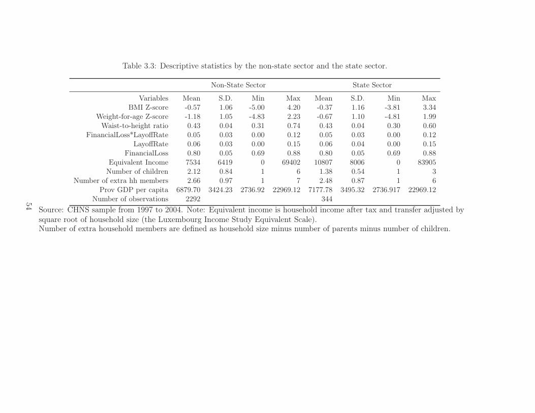
Table 3.3: Descriptive statistics by the non-state sector and the state sector.

Non-State Sector State Sector

Variables Mean S.D. Min Max Mean S.D. Min MaxBMI Z-score -0.57 1.06 -5.00 4.20 -0.37 1.16 -3.81 3.34

Weight-for-age Z-score -1.18 1.05 -4.83 2.23 -0.67 1.10 -4.81 1.99Waist-to-height ratio 0.43 0.04 0.31 0.74 0.43 0.04 0.30 0.60

FinancialLoss*LayoffRate 0.05 0.03 0.00 0.12 0.05 0.03 0.00 0.12LayoffRate 0.06 0.03 0.00 0.15 0.06 0.04 0.00 0.15

FinancialLoss 0.80 0.05 0.69 0.88 0.80 0.05 0.69 0.88Equivalent Income 7534 6419 0 69402 10807 8006 0 83905

Number of children 2.12 0.84 1 6 1.38 0.54 1 3Number of extra hh members 2.66 0.97 1 7 2.48 0.87 1 6

Prov GDP per capita 6879.70 3424.23 2736.92 22969.12 7177.78 3495.32 2736.917 22969.12Number of observations 2292 344

Source: CHNS sample from 1997 to 2004. Note: Equivalent income is household income after tax and transfer adjusted bysquare root of household size (the Luxembourg Income Study Equivalent Scale).Number of extra household members are defined as household size minus number of parents minus number of children.

54

Table 3.4: Continuous Difference-in-Difference Estimates with Individual Fixed Effects. Full Sample.

BMI Z-score Weight-for-age Z-score Waist-to-height ratio

Boy Girl Boy Girl Boy GirlSpecification 1 (1) (2) (3) (4) (5) (6)

FinancialLoss*Layoff rate*State 13.15** 14.52 8.955** 3.061 0.495* 0.62[3.953] [9.679] [2.713] [8.673] [0.221] [0.353]

FinancialLoss*Layoff rate -4.453** -3.780** -0.456 0.211 -0.18 -0.125[1.300] [1.593] [0.525] [1.450] [0.121] [0.176]

Log eq hh income 0.0264 -0.0658 0.00358 -0.0295 0.00176 -0.00655*[0.0373] [0.0496] [0.0317] [0.0463] [0.00177] [0.00296]

Other Controls Yes Yes Yes Yes Yes YesObservations 1,505 1,244 1,545 1,283 1,473 1,231

R-squared 0.043 0.035 0.015 0.058 0.069 0.051Number of IDind 954 826 972 845 948 825

Specification 2FinancialLoss*State -1.542 -1.479 3.093** 0.431 -0.0222 0.0343

[3.054] [2.762] [1.189] [3.969] [0.102] [0.115]Layoff*State 9.140* 9.985 8.016*** 1.816 0.359** 0.474

[3.901] [6.958] [1.872] [6.402] [0.150] [0.267]Financial Loss -0.0329 0.171 -0.222 -2.493* 0.123 0.164*

[1.419] [1.095] [2.089] [1.139] [0.0660] [0.0834]Layoff Rate -3.282** -2.667 -0.213 -0.963 -0.0682 -0.00596

[1.385] [1.488] [1.089] [0.943] [0.0731] [0.161]Log eq hh income 0.0276 -0.0707 0.00139 -0.0353 0.00187 -0.00626*

[0.0371] [0.0517] [0.0307] [0.0431] [0.00168] [0.00296]Other Controls Yes Yes Yes Yes Yes Yes

Observations 1,505 1,244 1,545 1,283 1,473 1,231R-squared 0.043 0.036 0.018 0.066 0.078 0.062

Number of IDind 954 826 972 845 948 825

Note: Robust standard errors clustered in provincial level in brackets. *** p<0.01, ** p<0.05, * p<0.1 Layoff rate andfinancial loss are recent 3-year average at provincial level. Other controls include number of children in households, numberof extra household members and GDP per capita in province. A constant is included. The sample consists of families withchildren in the state sector and non-state sector from 1997 to 2004 for 7 provinces in CHNS dataset.

55

Table 3.5: Continuous Difference-in-Difference Estimates with Individual Fixed Effects. Never lose job sample.

BMI Z-score Weight-for-age Z-score Waist-to-height ratio

Boy Girl Boy Girl Boy GirlSpecification 1 (1) (2) (3) (4) (5) (6)

FinancialLoss*Layoff rate*State 6.137* 7.776 9.952 2.357 -0.174 0.680**[3.155] [9.754] [6.076] [11.59] [0.101] [0.217]

FinancialLoss*Layoff rate -4.334** -2.111 -0.428 0.746 -0.320** -0.203[1.248] [1.139] [2.040] [1.761] [0.112] [0.145]

Log eq hh income 0.0803** 0.0425 0.026 0.0337 0.00299 -0.00174[0.0312] [0.0743] [0.0276] [0.0437] [0.00197] [0.00123]

Other Controls Yes Yes Yes Yes Yes YesObservations 1,024 860 1,050 878 1,003 849

R-squared 0.052 0.023 0.034 0.077 0.122 0.026Number of IDind 679 596 690 605 673 596

Specification 2FinancialLoss*State 7.768*** -2.291 1.823 -0.0621 0.310* 0.0129

[1.562] [4.584] [2.260] [5.081] [0.152] [0.0867]Layoff*State 10.60*** 4.689 8.71 0.619 0.039 0.519**

[2.346] [6.764] [4.874] [8.657] [0.193] [0.165]Financial Loss -1.948 -0.486 -1.676 -2.505*** 0.137 0.0654

[1.267] [1.388] [2.299] [0.647] [0.0816] [0.0638]Layoff Rate -4.258** -1.762 -1.095 -0.778 -0.151* -0.103

[1.280] [1.291] [2.190] [0.795] [0.0682] [0.141]Log eq hh income 0.0795** 0.042 0.029 0.0366 0.00259 -0.00189

[0.0265] [0.0730] [0.0262] [0.0425] [0.00193] [0.00128]Other Controls Yes Yes Yes Yes Yes Yes

Observations 1,024 860 1,050 878 1,003 849R-squared 0.059 0.025 0.04 0.088 0.146 0.028

Number of IDind 679 596 690 605 673 596

Note: Robust standard errors clustered in provincial level in brackets. *** p<0.01, ** p<0.05, * p<0.1 Layoff rate andfinancial loss are recent 3-year average at provincial level. Other controls include number of children in households, numberof extra household members (number of household members-number of children-number of parents), and CPI adjusted GDPper capita in province. A constant is included. The sample consists of families never lost or changed job with children inthe state sector and non-state sector with the exclusion of collective sector from 1997 to 2004 for 7 provinces in CHNSdataset.

56

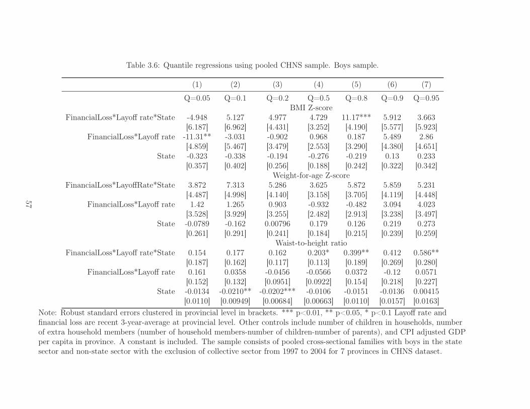
Table 3.6: Quantile regressions using pooled CHNS sample. Boys sample.

(1) (2) (3) (4) (5) (6) (7)

Q=0.05 Q=0.1 Q=0.2 Q=0.5 Q=0.8 Q=0.9 Q=0.95BMI Z-score

FinancialLoss*Layoff rate*State -4.948 5.127 4.977 4.729 11.17*** 5.912 3.663[6.187] [6.962] [4.431] [3.252] [4.190] [5.577] [5.923]

FinancialLoss*Layoff rate -11.31** -3.031 -0.902 0.968 0.187 5.489 2.86[4.859] [5.467] [3.479] [2.553] [3.290] [4.380] [4.651]

State -0.323 -0.338 -0.194 -0.276 -0.219 0.13 0.233[0.357] [0.402] [0.256] [0.188] [0.242] [0.322] [0.342]

Weight-for-age Z-scoreFinancialLoss*LayoffRate*State 3.872 7.313 5.286 3.625 5.872 5.859 5.231

[4.487] [4.998] [4.140] [3.158] [3.705] [4.119] [4.448]FinancialLoss*Layoff rate 1.42 1.265 0.903 -0.932 -0.482 3.094 4.023

[3.528] [3.929] [3.255] [2.482] [2.913] [3.238] [3.497]State -0.0789 -0.162 0.00796 0.179 0.126 0.219 0.273

[0.261] [0.291] [0.241] [0.184] [0.215] [0.239] [0.259]Waist-to-height ratio

FinancialLoss*Layoff rate*State 0.154 0.177 0.162 0.203* 0.399** 0.412 0.586**[0.187] [0.162] [0.117] [0.113] [0.189] [0.269] [0.280]

FinancialLoss*Layoff rate 0.161 0.0358 -0.0456 -0.0566 0.0372 -0.12 0.0571[0.152] [0.132] [0.0951] [0.0922] [0.154] [0.218] [0.227]

State -0.0134 -0.0210** -0.0202*** -0.0106 -0.0151 -0.0136 0.00415[0.0110] [0.00949] [0.00684] [0.00663] [0.0110] [0.0157] [0.0163]

Note: Robust standard errors clustered in provincial level in brackets. *** p<0.01, ** p<0.05, * p<0.1 Layoff rate andfinancial loss are recent 3-year-average at provincial level. Other controls include number of children in households, numberof extra household members (number of household members-number of children-number of parents), and CPI adjusted GDPper capita in province. A constant is included. The sample consists of pooled cross-sectional families with boys in the statesector and non-state sector with the exclusion of collective sector from 1997 to 2004 for 7 provinces in CHNS dataset.

57

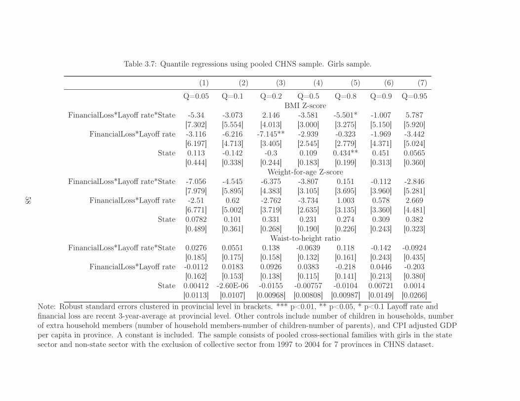
Table 3.7: Quantile regressions using pooled CHNS sample. Girls sample.

(1) (2) (3) (4) (5) (6) (7)

Q=0.05 Q=0.1 Q=0.2 Q=0.5 Q=0.8 Q=0.9 Q=0.95BMI Z-score

FinancialLoss*Layoff rate*State -5.34 -3.073 2.146 -3.581 -5.501* -1.007 5.787[7.302] [5.554] [4.013] [3.000] [3.275] [5.150] [5.920]

FinancialLoss*Layoff rate -3.116 -6.216 -7.145** -2.939 -0.323 -1.969 -3.442[6.197] [4.713] [3.405] [2.545] [2.779] [4.371] [5.024]

State 0.113 -0.142 -0.3 0.109 0.434** 0.451 0.0565[0.444] [0.338] [0.244] [0.183] [0.199] [0.313] [0.360]

Weight-for-age Z-scoreFinancialLoss*Layoff rate*State -7.056 -4.545 -6.375 -3.807 0.151 -0.112 -2.846

[7.979] [5.895] [4.383] [3.105] [3.695] [3.960] [5.281]FinancialLoss*Layoff rate -2.51 0.62 -2.762 -3.734 1.003 0.578 2.669

[6.771] [5.002] [3.719] [2.635] [3.135] [3.360] [4.481]State 0.0782 0.101 0.331 0.231 0.274 0.309 0.382

[0.489] [0.361] [0.268] [0.190] [0.226] [0.243] [0.323]Waist-to-height ratio

FinancialLoss*Layoff rate*State 0.0276 0.0551 0.138 -0.0639 0.118 -0.142 -0.0924[0.185] [0.175] [0.158] [0.132] [0.161] [0.243] [0.435]

FinancialLoss*Layoff rate -0.0112 0.0183 0.0926 0.0383 -0.218 0.0446 -0.203[0.162] [0.153] [0.138] [0.115] [0.141] [0.213] [0.380]

State 0.00412 -2.60E-06 -0.0155 -0.00757 -0.0104 0.00721 0.0014[0.0113] [0.0107] [0.00968] [0.00808] [0.00987] [0.0149] [0.0266]

Note: Robust standard errors clustered in provincial level in brackets. *** p<0.01, ** p<0.05, * p<0.1 Layoff rate andfinancial loss are recent 3-year-average at provincial level. Other controls include number of children in households, numberof extra household members (number of household members-number of children-number of parents), and CPI adjusted GDPper capita in province. A constant is included. The sample consists of pooled cross-sectional families with girls in the statesector and non-state sector with the exclusion of collective sector from 1997 to 2004 for 7 provinces in CHNS dataset.

58

Table 3.8: Continuous Difference-in-Difference Estimates with Individual FixedEffects. Urban and rural sample.

UrbanVARIABLES BMI Z-score Weight-for-age Z-score Waist-to-height ratio

Boy Girl Boy Girl Boy Girl

FinancialLoss*LayoffRate*State 11.54 8.460 2.047 -4.515 0.0901 0.692*[11.56] [10.29] [3.992] [10.29] [0.726] [0.308]

FinancialLoss*LayoffRate -8.800 -9.536 0.122 -2.563* -0.0525 -0.248[6.500] [5.078] [4.400] [1.297] [0.363] [0.668]

Log eq income 0.0730 0.118 -0.00263 -0.0480* 0.00957** 0.00263[0.0692] [0.0717] [0.0347] [0.0233] [0.00353] [0.00753]

Number of extra hh members 0.201* 0.339 0.183*** 0.355** 0.00113 -0.000832[0.102] [0.188] [0.0304] [0.105] [0.00294] [0.0143]

puberty -0.0511 0.256 0.0308 0.244* -0.00676 0.00643[0.0508] [0.204] [0.124] [0.122] [0.00357] [0.00722]

Prov GDP per capita (in 2009) -9.13e-05*** -7.70e-05 -5.22e-05** -6.96e-06 -2.81e-06 -1.09e-06[2.52e-05] [5.46e-05] [1.70e-05] [1.68e-05] [1.50e-06] [3.60e-06]

Constant -0.794 -1.639 -1.156** -1.112*** 0.367*** 0.412***[0.508] [1.002] [0.358] [0.207] [0.0390] [0.0907]

Observations 327 277 328 280 324 276R-squared 0.106 0.095 0.065 0.101 0.077 0.030Number of IDind 197 180 198 182 199 181

RuralVARIABLES BMI Z-score Weight-for-age Z-score Waist-to-height ratio

Boy Girl Boy Girl Boy Girl

FinancialLoss*LayoffRate*State 22.89** 27.05* 17.54** 21.20 1.127** 0.964[8.304] [11.55] [6.408] [11.88] [0.414] [0.561]

FinancialLoss*LayoffRate -3.134 -5.314** 0.311 -1.778 -0.107 -0.195*[1.986] [1.627] [1.159] [1.690] [0.119] [0.0908]

Log eq income 0.0193 -0.0993* -0.00679 -0.0147 0.00181 -0.00942**[0.0499] [0.0482] [0.0451] [0.0338] [0.00162] [0.00303]

Number of extra hh members 0.186* 0.0774 0.109 0.0738 0.00383 0.00360[0.0903] [0.0672] [0.0745] [0.0523] [0.00420] [0.00733]

puberty -0.0285 0.483*** -0.0709 0.329*** -0.00983 0.0126***[0.165] [0.0727] [0.0760] [0.0463] [0.00683] [0.00162]

Prov GDP per capita (in 2009) -3.22e-05 -6.17e-05** 3.57e-05* 2.24e-05 -2.89e-06** -4.94e-06***[3.75e-05] [2.39e-05] [1.70e-05] [1.78e-05] [8.38e-07] [1.23e-06]

Constant -0.856 0.405 -1.645** -1.554*** 0.438*** 0.540***[0.574] [0.499] [0.593] [0.406] [0.0207] [0.0345]

Observations 1,123 899 1,139 907 1,074 865R-squared 0.034 0.103 0.035 0.132 0.103 0.096Number of IDind 722 604 728 606 702 589

Note: Robust standard errors clustered in provincial level in brackets. *** p<0.01, ** p<0.05, * p<0.1 Layoff rateand financial loss are recent 3-year average at provincial level. Other controls include number of children inhouseholds, number of extra household members (number of household members-number of children-number ofparents), and CPI adjusted GDP per capita in province. A constant is included. The sample consists of children inthe state sector and non-state sector with the exclusion of collective sector from 1997 to 2004 for 7 provinces inCHNS dataset. Estimated for rural and urban sample separately.

Results are highly consistent after including time trend, secondary school enrolment rate, birth rate, employment

in non-state, population, and urban disposable income (in 2009 yuan)

59

Figure 3.1: Child capacity as a function of parental economic insecurity for differ-ent levels of expected economic loss.

Note: Figure 1 presents the child’s human capital formation as a function ofparental economic insecurity. Group 1 is experience no change in economic inse-curity. Group 2 experiences a mild increase in economic insecurity. Group 3 expe-riences a high increase in economic insecurity.

60

Figure 3.2: BMI growth charts for 5 to 19-year-olds from the World Health Orga-nization.

Source: http://www.who.int/growthref/

61

Figure 3.3: Density distribution of child outcomes in the CHNS sample.

Note: The sample consists of families with children in the state sector andnon-state sector with the exclusion of collective sector from 1997 to 2004 for 7provinces in CHNS dataset. The blue lines in BMIZ-score, weight for height Z-score, and waist to height ratio show kernel density plots.

62

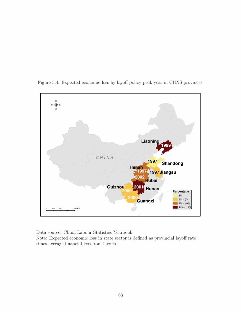
Figure 3.4: Expected economic loss by layoff policy peak year in CHNS provinces.

0 650 1,300325 Km

-

Percentage3%4% - 6%7% - 10%11% - 13%

C H I N A C H I N A

Jiangsu

Liaoning

ShandongHenan

HubeiHunan

Guangxi

Guizhou

1999

1997

2001

20002000

20021997

1997

Data source: China Labour Statistics Yearbook.Note: Expected economic loss in state sector is defined as provincial layoff ratetimes average financial loss from layoffs.

63

Figure 3.5: Level of economic insecurity by province and year, decomposed.

0%40

%80

%0%

40%

80%

0%40

%80

%

96 97 98 99 00 01 02 03 04

96 97 98 99 00 01 02 03 04 96 97 98 99 00 01 02 03 04

Liaoning Jiangsu Shandong

Henan Hubei Hunan

Guangxi Guizhou

Fina

ncial

Los

s

year

Financial Loss0%

5%10

%15%

0%5%

10%1

5%0%

5%10

%15%

96 97 98 99 00 01 02 03 04

96 97 98 99 00 01 02 03 04 96 97 98 99 00 01 02 03 04

Liaoning Jiangsu Shandong

Henan Hubei Hunan

Guangxi Guizhou

Layo

ff Ra

te

year

Layoff Rate

Data source: China Labour Statistics Yearbook.The layoff rate is defined as the number of state sector laid off workers at year end divided bythe number of state sector workers at the year end. Annual financial loss is defined as one minusthe off-post state sector worker living subsidy divided by average salary of on post state sectorworkers at provincial level.

64

Figure 3.6: Parallel trend in child outcomes: State sector V.S. Non-state sector.

Note: The sample consists of all families with 0 to 19-year-old children in the statesector and non-state sector with the exclusion of collective sector from 1991 to2006 for 7 provinces in CHNS dataset. The solid line represents the average of theoutcome in the state sector; the grey area represents its 95% CI. The dash repre-sents non-state sector, and its shaded area indicates the 95% CI. For all four out-comes, the state sector and the non-state sector present the same trend before thereform. The trends diverge during the reform, and converge after the reform.

65

Figure 3.7: The coefficient of EconomicLoss · Layoff · state on children’s BMIZ-score, Weight-for-age Z-score, Waist-to-height ratio over quantiles.

Note: The blue line indicates the coefficient of EconomicLoss · Layoff · state onthe vertical axis with the corresponding quantile on the horizontal axis. The 95%CI is shown in the shaded area. The coefficient and 95% CI in OLS are shown asthe horizontal lines.

66

Chapter 4

Gender Bias Within Chinese Families—Who Eats First in

Tough Times?

“Food consumption in particular has been shown to serve as a symbol or a code, de-

scribing certain human relationships, such as inclusion and exclusion, and intimacy

and distance. Eating may also tell us about ourselves for eating is a rutted habitua-

tion that is so close to the core of our memories, to the formation of our character

and the launching of our conscious experience, that its substances may be said to

become a part of us.”

—Bernadine Chee, 2000

4.1 Introduction

This chapter investigates the intra-household effects of negative income shocks on

nutrition intakes of Chinese boys versus girls; mothers versus fathers; and chil-

dren versus parents. Specifically, when an income loss occurs, whose food intake

decreases most?

China has a long history of privileging male children. Parents treat the food their

sons eat as a reflection of their improved economic status of the family, and no

other mode of parent-child interaction communicates their love for their sons more

than food (Jing, 2000). Many families, especially in rural areas, still treat sons as

their own family members, while daughters will eventually be “married off”, and

leave the families. Therefore, it is common for parents to allocate income and re-

sources from the daughter to son, especially when under a negative income shock

when resources become scarce. Furthermore, sons are expected to support the par-

ents when parents enter old age, especially in rural China. According to the China

National Bureau of Statistics data in 2005, pensions cover 4.6% of elderly support

in the rural area, while family support accounts for 54.1% (Dorfman et al., 2013).

The majority of the old-age support is from private resources. Parents have the

67

incentive to invest in sons, thus directly investing in their future pension. Son-

priority could also be explained by the gender imbalance and the high competition

faced by boys. The marriage rate of men in China is positively correlated with so-

cioeconomic status, and females are equally likely to get married regardless of their

socioeconomic status. Parents therefore are more likely to have higher expectations

on their sons’ performance and thus will allocate more food to their sons.

This chapter fills three areas that are understudied in the literature. First, it is

well-established that economic stress causes obesity (e.g. Smith, 2009; Offer, Pechey,

& Ulijaszek, 2010; Rohde, Tang, & Osberg, 2017; Watson, Osberg, & Phipps, 2016)

but the channel of the weight-gain is unclear. This chapter examines the dietary

changes under economic stress, which contributes to the relationship between obe-

sity and economic conditions. Second, the existence of intra-household inequality

is acknowledged as a problem in all societies, but few studies have investigated it

due to the scarcity of data on resource allocation within households. This chap-

ter uses food intake, which is one of the most important kinds of resource in Chi-

nese culture (Chee, 2000), to infer the inequality between boys and girls, fathers

and mothers, and parents and children. Third, the effects of economic anxiety on

health outcomes are mainly focused on adults, and little attention has been paid

to children (except for Kong & Phipps, 2016). I investigate the effects of negative

income shock on not only adults but also on the children. The finding has strong

policy implications, as it suggests that families switch from the primary resource

(protein) to an inferior resource (carbohydrate), which could affect children’s devel-

opment.

Novelties of this study include the following: 1) This chapter provides the rare ex-

amination, if not the first, of full range of family dynamics in intra-household allo-

cation of a scarce resource. 2) It observes 32,44 groups of siblings of mixed-sex in

the same families as well as their parents in 12 provinces from 1991 to 2011 and

followed them up to 5 times. 3) Son and daughter pairs within the households

are compared to infer intra-household resource allocation. 4) The daily intakes

of macronutrients, summarized into protein, carbohydrates, fat and energy cate-

gories, are recorded respectively for both siblings and their parents. The categories

of nutrition intake shed light on not only the quantity but also the quality of the68

resource allocation. 5) The level of daily intake is adjusted for age- and gender-

specific international standards.

The main purpose of the study is to investigate the gender inequality within house-

holds using nutrition distribution. It enriches the literature that examines the

changes in nutrition intakes in response to a negative income shock within the

household, as well as documents the macronutrient intakes of Chinese children and

their parents, especially compared to international standards.

4.2 Related literature

The study of inequality often neglects inequality among household members (Bur-

ton, Phipps, & Woolley, 2007). Equal sharing of income, consumption, resource

and well-being within the household is commonly assumed. However, a growing

number of studies point out the importance of intra-household allocation. For ex-

ample, Phipps and Burton (1995) discover that individual well-being is sensitive

to income-sharing assumptions. Lise and Seitz (2011) estimates that the Gini co-

efficient could increase by 30% after accounting for consumption inequality within

U.K. households.

Even if the existence of household inequality is recognized, the study of intra-household

inequality is largely restrained by the data availability as the income is usually col-

lected at household level (Osberg, 2000). Researchers have adopted different di-

mensions such as time, consumption, health and satisfaction to estimate the in-

equality within the household. For example, Burton, Phipps, and Woolley (2007)

include home production in income inequality. Phipps, Burton, and Osberg (2001)

demonstrate the inequality of free time for self among dual-earner households,

and women are more likely stressed about weekly hours, despite the total hours of

labour supply. Osberg (2015b) uses self-reported food deprivation in Tanzania and

finds the elderly rural women are more likely to suffer from hunger. He highlights

the gendered intra-household inequality and the demonstrates the importance of

including such inequality into poverty measurements and pension designs.

Apart from inequality between spouses in the household, intra-household inequal-

ity also exists between parents and children, as well as sons and daughters. Lund-

berg, Pollak, and Wales (1997) shows an increase in children’s clothing expenditure69

if the family allowance is directly paid to mothers. Burton, Phipps, and Woolley

(2007) use the age difference between couples in the eligibility of receiving the Old

Age Security in Canada, and the result suggests that the increase in women’s in-

come leads to a larger expenditure on gifts (possibly to grandchildren). Haddad

and Hoddinott (1994) uses data from Cote D’Ivoire and discover that an increase

in women’s cash income leads to an increase in boys’ height-for-age relative to

girls’. Duflo (2000) uses the expansion of the Old Age Pension program in South

Africa and finds an improvement in girls’ health and nutrition. To my knowledge,

most research on intra-household inequality uses exogenous increases in income to

investigate the resource allocation. Few studies have been done using an income

fall.

I am particularly interested in food intake for three reasons. First, nutrition dur-

ing childhood has long-term effects on the development of cognitive skills and the

productivity later in life (e.g. Dasgupta, 1995). Such effects are particularly im-

portant in developing countries (Duflo, 2000). Second, Chinese culture is highly

food-oriented (Chang, 1977), and food serves as a symbolic value of love. The pro-

cess of deciding which foods to eat, who will eat them, and how much to eat pro-

vides a path to understanding their everyday lives, and draws a vital picture of

their relationship with other people. The food allocation shapes the family dynam-

ics between parents and children, sons and daughters, reflecting the pleasures and

pressure of family members (Chang, 1977),.

Third, people of different cultures, geographies, and ethnicities eat different food

and have different ways to prepare and cook food. For example, southern Chinese

people tend to eat rice and favour sweet flavours, while northern Chinese cuisine

features wheat and a salty flavour. Western Chinese cuisine serves hot and spicy

meat based dishes. The differences in the food items, flavour, and cooking methods

can all be measured in calories, carbohydrates, proteins, and fats. Such measures

make them comparable resource indicators across culture, ethnicity, and economic

status and over time1.

1In the fixed effects estimation, I examine the changes in macronutrient intakes are examinedwithin the same household. Energy, carbohydrate, protein, and fat intakes provide comparablemeasures of resource allocation.

70

Despite the emphasis on food in Chinese culture, only a few studies have exam-

ined food intake in China. For example, Jing (2000) adopts a sociology perspec-

tive and conducts case studies in municipalities such as Beijing and Xi’an to por-

tray the changes in food intake under the rapid socioeconomic development of

China. Chang (1977) examines the evolution of food culture over the history of

five thousand years. The only quantitative research has been done focused on child

food intake in contemporary China at a national level is Cui and Dibley (2012).

They present the trend of dietary intake of Chinese children aged 7 to 17 using the

China Health and Nutrition Survey (CHNS) data. They show a steady decline in

energy and carbohydrate intake, and a steady increase in fat intake from 1991 to

2009. The value of daily protein intake decreases, but the ratio of protein-energy

ratio increases slightly. However, Cui and Dibley (2012) mainly focus on the nutri-

tion transition to a fat diet, and do not examine the income changes, sibling dis-

parity, and parent-child interactions.

Past literature has linked stress with changes in eating behaviour. Smith (2009),

Offer et al. (2010) and Köster and Mojet (2015), among other studies, describe

food that is high in fat and carbohydrates as comfort food, and is served as self-

medication; providing immediate relief from negative emotions. In other cases,

Macht (2008), Köster and Mojet (2015), and Staudigel (2016) discover that stress

could also reduce appetite and food intake. The bi-directional effects of emotion

show that stress controls, suppresses, impairs, regulates, or harmonizes eating be-

haviour. On average, Macht (2008) shows that emotional stress induces 30% peo-

ple to increase while 48% people to decrease in food intake using survey data. Staudi-

gel (2016) uses Russian panel data and demonstrates economic insecurity reduces

women’s body weight. He also discovers a strong link between economic insecurity

and sugar consumption.

In the Chinese context, Liu et al. (2007) examines the relationship between types

of food consumed by college students in seven cities and their stress and depression

measures. They find that the consumption of ready-to-go food (such as instant

noodles, frozen, canned or microwavable foods), snack foods (such as potato chips,

corn chips and tortilla chips) and fast food (such as McDonald’s, KFC, Pizza Hut)

is positively correlated with perceived stress level depression scores. They do not

71

establish the causal relationship between stress and eating behaviour. No research

thus far examines the intergenerational dietary change resulted from economic

stress. This chapter is also the first study in Chinese context to examine the di-

etary change of parents and children in response to an economic shock.

4.3 Data

4.3.1 The CHNS dietary intake data

The data of analysis are from the China Health and Nutrition Survey (CHNS)

from 1991 to 2011 (eight cycles). The CHNS is the only large-scale longitudinal

data set (Popkin et al., 2010) conducted by the Carolina Population Center at the

University of North Carolina at Chapel Hill and the National Institute of Nutrition

and Food Safety at the Chinese Center for Disease Control and Prevention. It cov-

ers 12 provinces that vary in geography, demographics and socioeconomic develop-

ment (China Health and Nutrition Survey, 2017). Figure 4.1 presents the provinces

that are covered by the CHNS data. Within each province, the sample is strati-

fied by one low-, two middle- and one high- per-capita income county or city. The

township capital and three villages in the county or the urban and suburban areas

in the city are randomly selected. Twenty households are then randomly selected

for the survey. All household members are interviewed. Children younger than 10

years old are assisted by parents. Community, household, and individual level data

are collected. The CHNS is representative of more than half of the population in

China. There are 12,944 households and 16,066 children in the 1991 cycle. In 2011,

there are 15,508 households and 22,977 children in the survey.

The CHNS hosts several features that make it particularly attractive for this study.

First, the longitudinal nature of the data enables me to observe families for up to

14 years 2 During the 14 years, the rapid economic development accompanied by

the economic reforms takes place and creates a rare opportunity to study negative

income shocks. In the data 11.6% of the sample, which amounts to 646 children,

experience large negative income shocks (defined as 25% of income loss). Second,

the CHNS not only provides information on the household heads, but also every2The CHNS panel runs from 1991 to 2011. The number of occurrences is also restrained by

the age of the child in the sample (2 to 17 years).

72

household member, including fathers, mothers, sons and daughters. The ability to

identify the relationship of household members enables studies on intra-household

dynamics and inequality. Third, the wide range of survey sample of 12 provinces

with both urban and rural areas enables me to observe 3,244 families with children

of mixed-sex, which is a rare find in China under the One Child Policy. Fourth,

the CHNS collects dietary intake information of all household members over the

course of three days. The collection of dietary intakes is on a 24-hour-recall basis,

and employs strict measures of changes in food stock, making the data quality ob-

jective and precise. The detailed information of dietary intake data collection and

calculation is the following:

Food intake is measured at the household level as well the individual level (i.e.

both children and parents) over three consecutive days of the survey. The three

survey days are randomly distributed across seven days of a week. The household

level of food intake is calculated by the change in food inventory from the begin-

ning to the end of each day. It is measured with a weighing and measuring tech-

nique using Chinese balance scale ranging from 20 grams (1 liang) to 15 kilograms

(30 jin). The nutritionists measure all the food items before the initiation of a 3-

day survey period (a0), all purchases and home production (a1) during the survey

period, and the food discarded and remaining food at the end of each day (a2).

The food consumption of household level is therefore defined as a0 + a1 − a2.

Every household member reports all food consumed at home and away from home

on a 24-hour recall basis3. Mothers or caregivers who handle food preparation are

asked to recall the food consumption of children younger than 12 years old. Nu-

tritionists record the types of food and snacks, the method of cooking, as well as

the time and place of consumption. Mothers, or those who handle the food prepa-

rations, together with other household members provide information on shared

dishes to determine the amount of individual intake. More than 99% survey re-

spondents have reported full three days of data (China Health and Nutrition Sur-

vey, 2017).

3According to the CHNS, 12% breakfast, 11% lunch and 5% dinner are consumed away fromhome. Home cooking accounts for 70% to 80% during the three-day survey period.

73

To calculate the daily intake of macronutrients including carbohydrates, fat, pro-

tein, and energy, the 1991 Food Composition Table for China is used as an aver-

age amount on a dish-by-dish basis for survey cycles prior to 2004. The 2002 Food

Composition Table is used in the subsequent surveys cycles of 2004, 2006, 2009

and 2011.

The CHNS implements strict quality control procedures. It follows the Declaration

of Helsinki, and the survey protocols, instruments, and process are approved by the

institutional review committees of the University of North Carolina at Chapel Hill.

The written consent was obtained from all survey respondents. The food intake

at the household level is matched with the individual level data. If a significant

discrepancy is found between the sum of individual level data and the household

data, the CHNS revisits the family to resolve the inconsistency. Field workers are

trained nutritionists who have post-secondary degrees and professional work ex-

perience in nutrition. The CHNS also provides three days of training on dietary

data collection to the field workers before the survey (China Health and Nutrition

Survey, 2017).

4.3.2 Dietary Reference Intakes (DRIs)

I use the Dietary Reference Intakes (DRIs)4 to adjust for the nutrient needs ac-

cording to the growth of children and the gender- and age-specific requirements for

parents (see Table 4.1). The DRIs table is developed by the Institute of Medicine

at the National Academies of Sciences Engineering Medicine and is widely used in

many international studies including the U.S. Guidelines for Americans, National

Health and Nutrition Examination Survey and the Canadian Community Health

Survey. It provides guidelines in daily consumption of energy, carbohydrate, pro-

tein and fat intakes for 97% to 98% of healthy individuals to meet nutrient require-

ments. The values are based on the recommended Physical Activity Level (PLA)

of 1.6 to 1.7 in healthy individuals, which means the total energy consumption is

60% to 70% of the resting energy expenditure, and it is equivalent of 60 minutes

of daily physical activity (Trumbo et al., 2002). The DRIs also take into account

4There are other food intake standards, such as the adult equivalence scale of food energyintake as adopted in Osberg (2015b). The advantage of the DRIs standards is that it providesnot only the overall calorie intakes but also the protein, carbohydrate, and fat intakes.

74

pregnant and lactating women, as these special stages require higher levels of nu-

trition intake. The adjustments are used when the analysis is done for children’s

mothers in the later section.

The dependent variable is children or parents’ percentage deviation in macronutri-

ent intakes from the DRIs in the age- and gender-specific group5.

IntakeDevi = (Intakei −DRIs)/DRIs (4.1)

Table 4.2 shows summary statistics using the pooled sibling sample (with and

without negative income shocks). A high-carbohydrate and low-protein diet is

found in boys, girls, fathers and mothers. For example, the carbohydrate intake

is 152.9% for boys and 138.7% for girls relative to the DRIs standards, while the

protein intake is only 70.3% for boys and 59.7% for girls. This result is consistent

with previous findings of lower protein-energy ratios in developing countries (Mill-

ward & Jackson, 2003). The overall energy intake is 110.7% for boys and 99.8% for

girls. The fat intakes are 60.2% for boys and 51.5% for girls.

In all macronutrient categories, consistently lower intakes of girls are observed

compared to boys in the same families with gaps ranging from 9 to 15 percentage

points. Their parents’ nutrition intakes exhibit the similar patterns as the children.

On average, fathers of boys’ energy intake is 169.3% while mothers of boys’ intake

is 143.5%. The discrepancy highlights gender differences in dietary intakes among

parents.

Table 4.2 also validates the sample of selection for boys and girls. Statistically

identical results are shown between the parents of girls and the parents of boys.

For example, when comparing the energy intake for mothers of boys to mothers’ of

girls, the average is 143.5% for both. The result suggests that the girls and boys

are selected from the statistically identical sample.

4.3.3 Negative income shock and its reasons

Hacker et al. (2014) propose the “Economic Security Index” using the frequency of

a 25% decline in individual net CPI-adjusted income from one year to the next.5The raw intakes are trimmed so that the observations above the top and below bottom 1%

are equal to the top and the bottom 1% respectively.

75

I adopt this criterion of a “large” income shock and define the negative income

shocks as the equivalent income loss (from all sources) more than 25% of the av-

erage of most recent three income observed6.

NegShockit = 0 ifYit − Yi

Yi

> −0.25;

NegShockit = 1 ifYit − Yi

Yi

≤ −0.25 (4.2)

where Yit is equivalent income of current cycle (i.e. family income from all sources

divided by square root of household size); and Yi = (Yit + Yit−1 + Yit−2)/3. Data are

trimmed so that negative income is equal to zero. I ignore negative income because

many families who are in business, farming, gardening, fishing, or raising livestock

report negative income. The nature of such business is to invest for a few years

and thus generating negative income, but a large return in the future is expected

(China Health and Nutrition Survey, 2017).

Types of economic risks

Osberg (1998) outlines four aspects of economic risks identified in the United Na-

tions’ Universal Declaration of Human Rights: unemployment, illness, family dis-

solution, and old age. In the CHNS data, the four risks can be identified by the

following questions:

• Unemployment: Changed or lost jobs since the last survey.

• Illness: Self-reported health of 1 or 2 on a 4-point scale, or self-reported hy-

pertension, diabetes, myocardial diseases, stroke or cancer.

• Family dissolution: Single, divorced, widowed or separated.

• Old age: male older than 60 and female older than 557

For simplicity, the child is coded in the category if either parent is in the category.

Table 4.3 shows the percentage of children associated with each economic risk by6The 25% income fall from the recent three-year average may lead to a larger income shock

than from the previous year. I also examine the 25% income loss from the previous year and theresults are highly consistent.

7The average retirement age in China is 60 for men and 55 for women (Dorfman et al., 2013).

76

families with or without a significant negative income shock (25% of equivalent

income loss). For children who experience a negative income shock in the fam-

ily, 35% experience illness of parents, 17% have unemployment, 3% have family

breakups, and 0.3% have old aged parents. The families without negative income

shock have a lower economic risk in each category except for old age.

Dietary knowledge

The CHNS also asks respondents 12-year and older diet knowledge in the cycles

2004, 2006, 2009 and 2011. To infer the overall energy intake, fat, carbohydrates,

protein and body image, the five questions are selected: Do you strongly agree (5),

agree, neither agree nor disagree, disagree or strongly disagree (1) with the follow-

ing statements:

• Eating a large amount of sugar is good for health.

• Eating food high in fat is good for health.

• Eating a large amount of staple food is good for health.

• Eating a large amount of animal products (e.g. fish, poultry, eggs, and lean

pork) every day ia good for health.

• The heavier you are, the healthier you are.

Table 4.3 shows the mean and standard deviation of each question answered by

children in the families with and without negative income shock. Children experi-

encing a negative income shock rated higher for all questions compare to children

without a negative income shock.

4.3.4 Child sample

The sample of this study consists of children of 2 to 17-year-old8 in the survey

years of 1991 to 2011. The birth cohort of the children is from 1973 to 2009. In

8Children and infants who are younger than 2-year-old are likely breastfed and the dietaryintakes are thus incomparable.

77

the CHNS children sample, 36% of the children are from only-child families and

3,357 children have had one or more siblings of the opposite sex9.

I limit the sample of analysis to families with one or more child of the opposite

sex for sibling fixed effects analyses. At least one girl and one boy are observed in

each family, and at least two children are observed in each family in each nutrition

survey year. The sample consists of 3,243 children and 1,364 households, with 20%

of children observed four times, 28% three times, and 34% twice in the longitudinal

sample.

There are 2,667 boys and 2,908 girls in the sample (see Table 4.2). The average

birth order for boys is 1.9 and for girls is 1.6. The difference is statistically sig-

nificant, and it can be explained by the One Child Policy, which permits the sec-

ond birth in rural area if the first child is a girl. Other demographic variables are

consistent across genders. In the sample, 11.4% of boys and 11.8% of girls experi-

ence negative income shock (25% income decline than the average in recent three

cycles). On average, the equivalent household income is 7325 CPI-adjusted-2006

Yuan. Rural children account for 81% of the sample. On average, there are 2.5

children and 2.5 extra household members in a family. In the sample of analysis.

33% of children have completed primary schooling, and 20% have completed mid-

dle schooling. 43% of the children reached the age of puberty.

4.3.5 Siblings under the One Child Policy

How does the sibling sample in this study compare with the only-child sample?

Even under the China One Child Policy, siblings are still commonly observed in

Chinese families. Culturally and historically, Chinese families are in favour for hav-

ing more children. Mao Zedong, the chairman of China from 1949 to 1976, advo-

cated “more people, more power” and believed a rising population is a major drive

for economic growth. After Mao’s death in 1976, Deng Xiaoping took power. Deng

believed in population control and promoted the growth in GDP per capita. The

Chinese government thus enacted the One Child Policy in 1979 (Peng, 1991).

9I also investigate if the first borns are favoured in families with children of the same sex. Nosignificant patterns are found

78

The One Child Policy was resisted by Chinese families, especially in the rural ar-

eas. Starting in 1984 and 1985, the communist government relaxed the policy so

that rural families with one daughter could have a second child. The fertility rate,

therefore, rebounded from 1984 to 1986. Besides of the less stringent implemen-

tation in rural areas, the One Child Policy was also relatively relaxed in less de-

veloped provinces and ethnic minority groups. Figure4.2 shows the fertility rate

in the urban and rural area from 1973 to 2009. The fertility rates were 5 and 2.4

in the rural and urban area respectively in 1973, and the figures became 1.4 and

0.96 in 2009. Therefore, for the birth cohort of this study from 1973 to 2009, it is

common for Chinese families to have siblings.

Figure 4.3 presents mean and standard errors of percentage deviation of children’s

and parents’ macro-nutrient intake from the DRIs standards by gender and only-

child status. Protein intakes of Chinese children in all groups are significantly lower

than the international standard. Boys have more protein than girls in both only

child and non-only-child families. On average, Chinese boys in non-only-child fam-

ilies have 79% of the protein, comparing to Chinese girls in non-only-child families

having 68% of the protein using DRIs standards. In only-child-families, the pro-

tein intake is higher for both genders—83% for boys and 76% for girls. Fat intake

shows the same pattern as the protein intake with a smaller gap from the DRIs

standards. On the contrary, carbohydrate intakes of Chinese children are relatively

high, especially in non-only-child families. Boys with siblings consume 130% and

girls with siblings consume 120% of carbohydrates intake standard. Carbohydrate

intakes are 107% and 76% of the DRIs standards for only-child boys and girls re-

spectively. The total energy intake is highest among boys with siblings, and lowest

among only-child girls.

The shortage of protein intake and excess of carbohydrate intake are even more

prominent among parents. Fathers’ protein intakes range from 36% to 41% of the

international standard, while father’s carbohydrate intake is 1.7 to 2.4 times of

the international standard. Mothers, on average, consume 48% of protein, and 1.7

times carbohydrates of the DRIs standards. Both mothers and fathers consume

smaller amounts of fat in non-only-child families than those in only-child families,79

but higher total energy intakes contributed by high carbohydrate intakes10.

4.4 Empirical framework

4.4.1 Sibling fixed effect model

In economic literature, most studies on children estimate child outcomes on a set

of observables of family and child characteristics. Two concerns are raised by this

approach, unobserved heterogeneity and income endogeneity (Dahl & Lochner,

2012). Mayer (1997), among others, suggests that the estimation omits unobserved

heterogeneities across households. For example, children’s outcomes could be driven

by factors (neighbourhood, family environment and child’s ability) other than in-

come. In the Chinese context, the One-Child Policy boosted gender selection prac-

tice using ultrasound technology since its introduction in the 1980s (Chen et al.,

2013). The availability of gender-selected abortions differs across provinces, urban

or rural, economic status and family values, which contributes to the selection bias

of girls and boys families. It is possible that girls may be more likely from disad-

vantaged families because their families cannot afford ultrasound scanning or abor-

tions.

To remove the permanent unobserved family and children characteristics, I use

sibling fixed effects as adopted by Blau (1999) and Levy & Duncan (2000).. I es-

timate the differences in dietary intakes between brothers and sisters within the

same households. Differences in family levels across siblings are removed when esti-

mating the impacts of negative income shocks on child outcomes. The fixed effects

model also enables me to compare the dietary intakes with and without negative

income shock, and thus estimating the changes in dietary intakes in response to

negative incomes. I employ three estimations on children, parents, and the combi-

nation of parent-children.

10I examine the intergenerational gender inequality among only-child families using propen-sity score matching, and found that the gender inequality is only significant among families withchildren of mixed-sex.

80

First, I estimate child dietary intakes with sibling fixed effects as follows:

IntakeDevijt = αj + β0NegShockjt ·Girlij + β1NegShockjt +Γ1Xjt +Γ2Wijt + εijt

(4.3)

where i indexes individuals (i.e. children in this equation), j indexes families, and

t indexes survey year. IntakeDev is percentage deviation of energy, carbohydrate,

fat and protein intake from the age- and gender-specific Dietary Reference Intake

standard. X is a vector of family-specific characteristics. W is a vector of observed

child-specific characteristics. Standard errors are clustered at the family level.

The sibling fixed effects are captured by αj, which reflect unobserved permanent

family characteristics.The hypothesis is that β0 < 0, which suggests in response to

negative income shocks, girls reduce their macronutrient intakes more than boys in

the same families.

Second, I examine the parents’ dietary intakes using the same children’s sample.

IntakeDevijt = αj+β0NegShockjt ·Motherij+β1NegShockjt+Γ1Xjt+Γ2Wijt+εijt

(4.4)

where i indexes individuals (parent in this equation). IntakeDevijt is percentage

deviation of the father or the mother’s energy, carbohydrate, fat or protein intake

from the DRIs standards. NegShockjt estimates the overall effects of negative in-

come shocks on both the father and the mother, and NegShockjt · Motherij cap-

tures the extra effects on the mother in the same household.

Third, I combine the child sample and the parent sample estimated above, and

test if parents shield their children from dietary reductions when economic hard-

ships strike. By estimating the dietary intakes of two generations, I can investigate

the resource reallocation among fathers, mothers, sons and daughters in the same

households.

IntakeDevijt = αj+β0NegShockjt ·Girlij

+β1NegShockjt ·Motherij

+β2NegShockjt · Fatherij

+β3NegShockjt + Γ1Xjt + Γ2Wijt + εijt (4.5)

81

where i indexes family members. The base of NegShock effects is boys, and the

interaction terms of NegShock with girls, mothers and fathers capture the extra

effects on each individual.

4.4.2 Other controls

For all sibling fixed effects estimation, I present 3 specifications. First specifica-

tion controls the number of children in the families, if there is/are grandparent(s)

or relatives present. The second specification adds if the child graduated from pri-

mary school or middle school, the birth order of the child, and if the child entered

puberty 11. The last specification adds the log equivalent income of the current pe-

riod12.

Figure 4.4 shows the means and standard errors of independent variables by child

gender and only-child status. There are 10% of non-only-child families in the pooled

sample experiencing negative income shock, while only 6% of only-child families

had negative income shock. The only-child and non-only child families differ in de-

mographic characteristics. According to Figure 4.4, only-child families have more

household members other than children and parents. There is a higher percentage

of only-children who completed middle school than non-only children. Equivalent

income is 7,738 for non-only-child families and 14,770 for only-child families. 80%

non-only child families and 59% of the only-child families are in rural area.

4.5 Results

4.5.1 Boys and girls’ intakes

Table 4.4 shows the estimates of child nutrition intake using sibling fixed effects.

The hypothesis is that negative income shocks affect boys’ intakes less than girls’,

i.e. sons are favoured during tough times. I examine three nutrition intakes, car-

bohydrates, fat and protein, as well as the overall energy intakes (the combina-

tion of the three nutrition). For each outcome, I use three specifications: the first

11Girls entering puberty if the answer is "Yes" to the question "Have you ever menstruated?"and boys entering puberty is defined as at 11 to 18 (Zhu et al., 2013).

12Equivalent income is defined as household income from all sources after tax and transfer in2006 Yuan divided by the square root of household size (Luxembourg Income Study, 2017).

82

one controls for time-variant household characteristics; the second one controls for

household characteristics and child-specific characteristics; and the third specifica-

tion adds the current equivalent income as control. While the variables of interests

are negative income shock and its interaction(s), equivalent income in fixed effects

model also captures the changes in income. Therefore, the second specification is

the preferred specification. The income variable is added in the third specification

to estimate the “extra” critical point effects of 25% income fall.

Column 1 in Table 4.4 shows energy intake of children increases in response to

a negative income shock, controlling for family characteristics. A 25% of income

shock increases energy intake by 9.9 percentage points in terms of the DRIs stan-

dards. After accounting for household and child characteristics, the interaction of

negative shock and girl becomes significant. Girls reduce their energy intake by 7

percentage points, while boys’ energy is not significantly affected.

Carbohydrate intake is also significantly affected by negative income shocks. Col-

umn 4 shows that carbohydrate intake increases by 21.3 percentage points for

boys, and by 13.9 (=0.213-0.074) percentage points for girls. After controlling for

child-specific characteristics, the estimation still shows a 12.4-percentage-point in-

crease in boys, but a 2.4-percentage-point decrease in girls. In the preferred speci-

fication in Column 6, a 14-percentage-point increase in boys, and a 0.5-percentage-

point decrease in girls is estimated after controlling for income.

The sibling fixed effects estimation shows that protein intake reduces for both girls

and boys when income falls 25% (see Columns 10-12, Table 4.4). With controls for

families observed and permanent unobserved characteristics, boys’ protein intakes

decrease by 15.2 percentage points, and girls’ protein intakes decrease by 24.9 per-

centage points. The magnitude of reductions is significant considering the average

of protein intake is only 70.3% of DRIs standard for boys and 59.7% for girls. The

results persist even after controlling for income. There is a 16-percentage-point de-

crease for protein intake for all children. The interaction term of negative shock

and girl becomes insignificant.

On the contrary to the previous finding of a positive relationship between fat diet

and economic insecurity, no change in fat intake of children is found due to nega-

tive income shocks.

83

Sample of adolescents

Adolescence is a critical transition period, and many biological, psychological and

social roles are formed during this life stage. It is the foundation of future devel-

opment (Sawyer et al., 2012). I limit the sample to adolescents and test if the gen-

der disparity is larger during this life period. The adolescent sample is defined as

girls from menstruation to 17-year-old and boys from 11-year old until 17-year-old

(World Health Organization, 2017). There are 1,391 boys and 1,005 girls in the

adolescent sample, which accounts for 43% of the full sibling sample13.

Table 4.5 presents the sibling fixed effects estimates of dietary intakes on negative

income shocks. Columns 1 to 3 show that daily energy intake is significantly re-

duced by 18.2 to 21.1 percentage points in the presence of negative income shocks

for girls, while no reduction of energy intakes for boys. This result is consistent

across three specifications. This result suggests a higher gender disparity among

adolescents than the previous estimate with full sibling sample.

Girls also experience a large decrease in carbohydrate intake. After controlling

for household and child-specific characteristics, the carbohydrate intake decreases

by 29.4 percentage points for girls. Boys, on the contrary, is estimated a 24.4-

percentage-point increase in carbohydrate intake in Column 6. After controlling

for income, girls still experience a 5-percentage-point of carbohydrate intake re-

duction, which is a 29.4-percentage-point difference between boys and girls. This

result suggests that the boys eat more and the girls reduce their carbohydrate in-

takes in response to a negative income shock.

Negative income shocks have negative effects on the fat intake of adolescent girls.

Columns 7 to 9 in Table 4.5 show the fat intake reduces by 18.2 to 20.1 percent-

age points for girls. Boys fat intake show no significant change. The average fat

intake for girls is only 51.5% of the DRIs standard, while for boys is 60.2% (see

Table 4.2). The reduction in fat intake due to the negative income shock puts ado-

lescent girls in a more disadvantaged diet than their boy counterparts.

The protein intake is estimated to be negatively affected by income shock for both

13I also examine the early childhood sample of 2-to-5-year-olds, as Heckman (2011) outlinesthe importance of invest in the early years. I do not find a significant gender disparity in thesample of early years.

84

genders (see Column 10 in Table 4.5). Boys’ protein intake is estimated to be re-

duced by 11.0 percentage points, while girls are expected to reduce a further 8.5%

in protein intake, totalling 19.5-percentage-point reduction. The effects on both

girls and boys become insignificant after controlling for income.

Overall, the estimates of the adolescent sample show a larger gender disparity be-

tween boys and girls within the household. In response to negative income shock,

girls in the adolescent sample intake 19.3 percentage points less of energy, 29.4 less

of carbohydrate, and 19.6 less of fat, compared to boys in the same households.

Considering girls have lower intakes than boys using the DRIs standards, the di-

etary reductions from the income loss is particularly problematic.

4.5.2 Fathers’ and mothers’ intakes

Table 4.6 presents the estimates of parents’ dietary intakes with family fixed ef-

fects. The hypothesis is that mothers take a larger dietary cut than fathers in re-

sponse to negative income shocks. The differential effects of negative income shock

between mothers and fathers are captured by NegShock ·Mother.

Columns 1 to 9 show negative coefficients of NegShock · Mother, which means

mothers reduce energy, carbohydrate, and fat intakes significantly more than fa-

thers. The estimates are highly consistent across three specifications. Compared

to fathers, mothers reduce 29 to 31 percentage points more in energy, 47 to 50

percentage points more in carbohydrates, and 25 to 27 percentage points more in

fat intakes in response to negative income shocks. The only exception is protein

intake. On average, a 6.02-percentage-point reduction is found in fathers protein

intake, while a 1.75 (=-0.0602+0.0427)-percentage-point reduction in mothers’ pro-

tein intake. There is no evidence of significant reduction in father’s dietary intakes

except for protein intakes. On the contrary, an increase in carbohydrate intakes

of 12.6 to 19.1 percentage points is found in specifications 1 and 2 (see Columns 4

and 5 in Table 4.6)

4.5.3 Parents’ and children’s intakes

Table 4.7 presents the family fixed effects estimates of both parents and children

using the same sample of siblings of mixed-sex. The coefficient of NegShock is the85

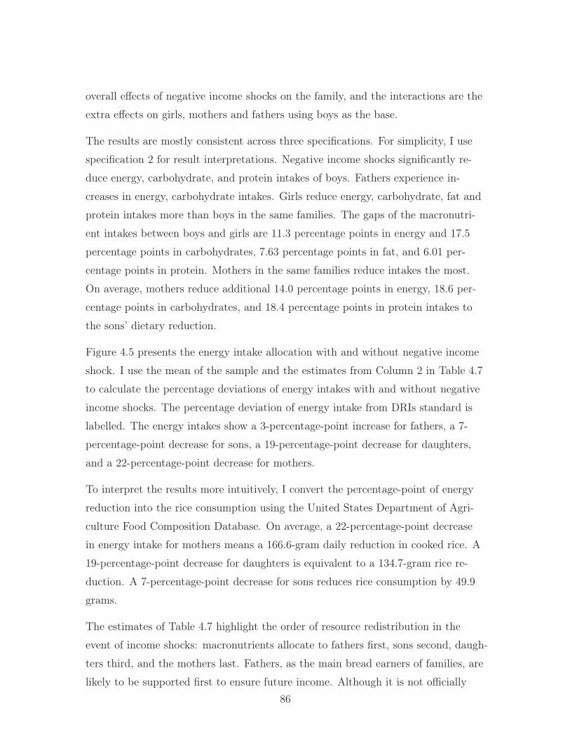
overall effects of negative income shocks on the family, and the interactions are the

extra effects on girls, mothers and fathers using boys as the base.

The results are mostly consistent across three specifications. For simplicity, I use

specification 2 for result interpretations. Negative income shocks significantly re-

duce energy, carbohydrate, and protein intakes of boys. Fathers experience in-

creases in energy, carbohydrate intakes. Girls reduce energy, carbohydrate, fat and

protein intakes more than boys in the same families. The gaps of the macronutri-

ent intakes between boys and girls are 11.3 percentage points in energy and 17.5

percentage points in carbohydrates, 7.63 percentage points in fat, and 6.01 per-

centage points in protein. Mothers in the same families reduce intakes the most.

On average, mothers reduce additional 14.0 percentage points in energy, 18.6 per-

centage points in carbohydrates, and 18.4 percentage points in protein intakes to

the sons’ dietary reduction.

Figure 4.5 presents the energy intake allocation with and without negative income

shock. I use the mean of the sample and the estimates from Column 2 in Table 4.7

to calculate the percentage deviations of energy intakes with and without negative

income shocks. The percentage deviation of energy intake from DRIs standard is

labelled. The energy intakes show a 3-percentage-point increase for fathers, a 7-

percentage-point decrease for sons, a 19-percentage-point decrease for daughters,

and a 22-percentage-point decrease for mothers.

To interpret the results more intuitively, I convert the percentage-point of energy

reduction into the rice consumption using the United States Department of Agri-

culture Food Composition Database. On average, a 22-percentage-point decrease

in energy intake for mothers means a 166.6-gram daily reduction in cooked rice. A

19-percentage-point decrease for daughters is equivalent to a 134.7-gram rice re-

duction. A 7-percentage-point decrease for sons reduces rice consumption by 49.9

grams.

The estimates of Table 4.7 highlight the order of resource redistribution in the

event of income shocks: macronutrients allocate to fathers first, sons second, daugh-

ters third, and the mothers last. Fathers, as the main bread earners of families, are

likely to be supported first to ensure future income. Although it is not officially86

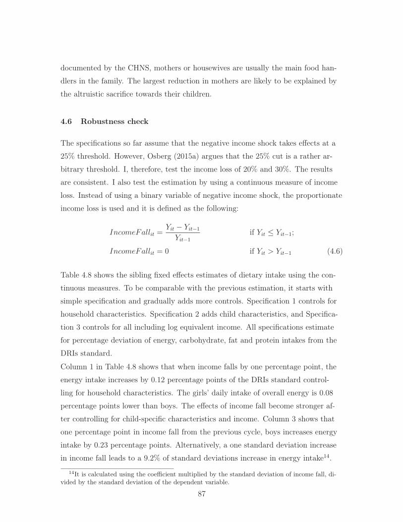
documented by the CHNS, mothers or housewives are usually the main food han-

dlers in the family. The largest reduction in mothers are likely to be explained by

the altruistic sacrifice towards their children.

4.6 Robustness check

The specifications so far assume that the negative income shock takes effects at a

25% threshold. However, Osberg (2015a) argues that the 25% cut is a rather ar-

bitrary threshold. I, therefore, test the income loss of 20% and 30%. The results

are consistent. I also test the estimation by using a continuous measure of income

loss. Instead of using a binary variable of negative income shock, the proportionate

income loss is used and it is defined as the following:

IncomeFallit =Yit − Yit−1

Yit−1if Yit ≤ Yit−1;

IncomeFallit = 0 if Yit > Yit−1 (4.6)

Table 4.8 shows the sibling fixed effects estimates of dietary intake using the con-

tinuous measures. To be comparable with the previous estimation, it starts with

simple specification and gradually adds more controls. Specification 1 controls for

household characteristics. Specification 2 adds child characteristics, and Specifica-

tion 3 controls for all including log equivalent income. All specifications estimate

for percentage deviation of energy, carbohydrate, fat and protein intakes from the

DRIs standard.

Column 1 in Table 4.8 shows that when income falls by one percentage point, the

energy intake increases by 0.12 percentage points of the DRIs standard control-

ling for household characteristics. The girls’ daily intake of overall energy is 0.08

percentage points lower than boys. The effects of income fall become stronger af-

ter controlling for child-specific characteristics and income. Column 3 shows that

one percentage point in income fall from the previous cycle, boys increases energy

intake by 0.23 percentage points. Alternatively, a one standard deviation increase

in income fall leads to a 9.2% of standard deviations increase in energy intake14.

14It is calculated using the coefficient multiplied by the standard deviation of income fall, di-vided by the standard deviation of the dependent variable.

87

Girls’ energy intake is significantly lower than boys. For one standard deviation of

income fall, girls energy intake increase by 2.9%.

Columns 3 to 12 in Table 4.8 break down the energy intake into types of macronu-

trient. The estimates of carbohydrate in three specifications show consistent posi-

tive effects from income fall as shown in row 2. %IncomeFall is positive, meaning

the income fall increases carbohydrate intake, and %IncomeFall*Girl is negative,

meaning the effects on carbohydrate intake is negative on girls compared to their

brothers. The preferred specification of Column 6 shows that a 100% income fall

increases carbohydrate intake by 42.1 percentage points for boys, and 15.3 percent-

age points (=0.42.1-0.268) in girls. In other words, one standard deviation decrease

in income, increases carbohydrate intake by 11.3% standard deviations in boys,

and 4.1% standard deviations in girls. Fat intakes are not statistically significant.

Protein intake is reduced in both genders, with a larger reduction in girls. A unit

of income fall leads to a reduction of protein intake by 0.255 units of for boys, and

by 0.378 (=-0.255-0.123) units for girls. If the income decreases by 1 standard de-

viation, the protein intake would decrease by 8.9% standard deviations for boys

and 13.2% standard deviations for girls.

Table 4.9 shows larger effects of income fall using adolescents sample. For one unit

of income fall, energy intake increases by 0.386 percentage points in boys, and

0.052 percentage points in girls; carbohydrate intake increases by 0.727 percent-

age points in boys, and 0.194 percentage points in girls. In other words, one stan-

dard deviation in income fall increase energy intake by 14.2% standard deviations

in boys, and 1.9% standard deviations in girls, and increase carbohydrate intake by

19.0% in boys, and 5.0% in girls. Changes in fat and protein intake are insignifi-

cant in the adolescent sample.

The estimates using the percentage income fall show that children’s food intake

and nutrition allocation is affected by the level of income fall continuously. The

average effects show that boys and girls increase the carbohydrate intake and de-

crease the protein intake in response to income losses. The increase in carbohy-

drate is less but the decrease in protein is more for girls.

I also test quadratic form of income loss. The quadratic term is not significant.

Besides the sample of children with siblings of opposite sex, I examine the children88

with siblings of the same sex. I do not find any dietary orders or patterns within

the families, such as the first-born preference.

4.7 Conclusion

This study draws the following conclusions. First, protein and fat intakes of Chi-

nese children are significantly lower, while carbohydrate and overall energy intakes

are higher, than the DRIs standard. In all four categories, girls have significantly

lower intake levels than boys, suggesting a gender disparity before the negative in-

come shocks take place. Second, in response to negative income, Chinese families

tend to reduce their protein intake, the primary macronutrient, possibly due to

a higher price. Third, adolescent girls experience a larger dietary reduction than

boys in energy, carbohydrate, and fat intakes.

The most compelling finding is that when families experience negative income

shocks, the resource is allocated in the order of fathers, sons, daughters and moth-

ers. Gender inequality is heightened in the event of income loss. The prioritizing

fathers and sons, while neglecting daughters and mothers show an increase in gen-

der disparity in response to large income loss. It draws concerns that economic

losses are likely to impede the development of daughters and obstructs the well-

being of mothers.

Birch and Fisher (1998) documents that eating behaviour during childhood and

adolescence can have significant influences on future food intake. Parental dietary

practices can alter dietary intake patterns, preferences for energy-dense foods, and

even the internal responsiveness to hunger and satiety in children and in future

adulthood. The phenomenon of “feeding the little emperor” in response to negative

income shocks in Chinese families is especially problematic for children’s future

development, and could contribute to unhealthy eating habits and adult obesity.

It is unclear that the differences in dietary intake are caused by parental control,

or if it stems from the children themselves. The gender difference could come from

the children themselves. Sons could be more expressive about their demands than

daughters. Girls, especially adolescent girls, may be more reserved about their re-

quests and “internalize” their demand. Also, sons may be more likely to demand

food, and girls may request resources other than food (e.g. clothing or beauty89

products). When dealing with children’s demands, parents may be more likely to

give in when they are under economic stress.

One of the limitations is that I focus on families with sex-mixed children. It is also

interesting to examine if father or mother would reduce more intakes in only child

families. Given the presence of grandparents and their involvements in child care

in China, the dietary intakes of grandparents could also be examined.

I only examine macronutrient intakes but not micronutrient intakes. Micronutri-

ents, such as vitamins and minerals, play an important role in the healthy devel-

opment of children. For future research, other dietary intakes could be examined

when such data are available.

Another direction of future research is to include the price of food in the analy-

sis. The CHNS provides detailed information on the price of rice, bread, meat, and

oil in the local market. It would be interesting to examine if the negative income

shock makes families opt out from expensive protein and opt in for cheap carbohy-

drate.

Apart from dietary intakes, it would be interesting to also examine time and con-

sumption allocation within the household. For obesity research, for example, time

spent in physical activity, TV and video games could be investigated and gender

differences could be explored. The consumption patterns, such as pocket money

(Ling Hua Qian) distribution and the frequency of western fast food restaurant

visits, are also worthy of attention.

90

Table 4.1: Dietary Reference Intakes (DRIs): Recommended Dietary Allowancesand Adequate Macronutrients Intakes

Carbohydrate Fat Protein EnergyGroup (g/d) (g/d) (g/d) calorieInfants0 to 6 mo 60 31 9 555.46 to 12 mo 95 30 11 694Children 01-3y 130 30 13 8424-8y 130 30 19 866Males 30 2709-13y 130 30 34 92614-18y 130 30 52 99819-30y 130 30 56 101431-50y 130 30 56 101451-70y 130 30 56 1014>70y 130 30 56 1014Females 30 2709-13y 130 30 34 92614-18y 130 30 46 97419-30y 130 30 46 97431-50y 130 30 46 97451-70y 130 30 46 974>70y 130 30 46 974Pregnancy 30 27014-18y 175 30 71 125419-30y 175 30 71 125431-50y 175 30 71 1254Lactation 30 27014-18y 210 30 71 139419-30y 210 30 71 139431-50y 210 30 71 1394

Source: Dietary Reference Intakes for Energy, Carbohydrate, Fiber, Fat, Fatty Acids, Cholesterol, Protein, andAmino Acids (2002/2005) and Dietary Reference Intakes for Water, Potassium, Sodium, Chloride, and Sulfate(2005). The report may be accessed via www.nap.edu.

Fat intake of 1 to 70-year-old is from Dietary Reference Intakes (DRIs): Acceptable Macronutrient Distribution

Ranges. The average of the range is used. Energy intake is calculated by the author using

Energy(calorie)=9xFat(g)+4xCarb(g)+4xProtein(g). Energy from alcohol intake is ignored from the calculation

because of lack of data. It is not likely to affect the estimation as the subject of the study is children of 2 to

17-year-old who are not likely to consume alcohol.

91

Table 4.2: Summary statistics of sibling sample of analysis

Boy GirlVARIABLES N Mean SD N Mean SD

Energy % dev 2,667 1.107 0.643 2,908 0.998 0.608Carb % dev 2,667 1.529 0.919 2,908 1.387 0.848Fat % dev 2,667 0.602 0.953 2,908 0.515 0.910Protein % dev 2,667 0.703 0.725 2,908 0.597 0.655Father Energy % deviation 2,488 1.693 0.726 2,699 1.696 0.736Father Carb % deviation 2,488 2.466 1.120 2,699 2.466 1.136Father Fat % deviation 2,488 1.088 1.162 2,699 1.102 1.197Father Protein % deviation 2,488 0.405 0.435 2,699 0.411 0.438Mother Energy % deviation 2,618 1.435 0.659 2,855 1.435 0.669Mother Carb % deviation 2,618 2.070 0.988 2,855 2.063 0.996Mother Fat % deviation 2,618 0.832 1.021 2,855 0.844 1.053Mother Protein % deviation 2,618 0.482 0.464 2,855 0.490 0.469%IncomeFall*Girl 2,362 0 0 2,563 0.124 0.240%IncomeFall 2,362 0.122 0.238 2,563 0.124 0.240NegativeShock*Girl 2,667 0 0 2,908 0.118 0.322NegativeShock 2,667 0.114 0.318 2,908 0.118 0.322Loss30 2,667 0.164 0.370 2,908 0.166 0.373Loss20 2,667 0.190 0.393 2,908 0.192 0.394Number of children 2,667 2.485 0.649 2,908 2.577 0.758Number of extra hh members 2,667 2.453 0.813 2,908 2.461 0.846Primary Schooling 2,667 0.313 0.464 2,908 0.338 0.473Middle Schooling 2,667 0.175 0.380 2,908 0.220 0.414Child at the age of puberty 2,667 0.522 0.500 2,908 0.346 0.476Birth order 2,667 1.915 0.845 2,908 1.600 0.771Equivalent Income 2,667 7,221 8,581 2,908 7,423 9,119Rural residents 2,667 0.814 0.389 2,908 0.813 0.390

Number of families 1,312 1,312 1,312 1,312 1,312 1,312Source: CHNS 1991 to 2011. Children 2 to 17 year old. Sample of children with siblings of opposite sex. At leasttwo children in one family are surveyed in one cycle.

Note: % dev of energy, carb, fat and protein is the percentage deviation of macronutrient intake from the age- and

gender-specific DRIs standards. Equivalent income is defined as household income after tax and transfer divided

by square root of household size. NegShock is defined as 1 if the equivalent income falls more than 25% from the

average of previous 3 cycles, 0 otherwise. Loss30, Loss25, Loss20 are defined as the income loss of 30, 25 and 20

percent from the previous cycle

92

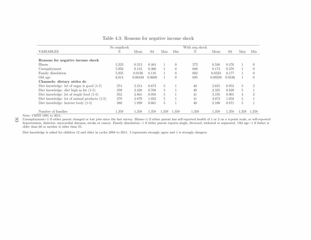
Table 4.3: Reasons for negative income shock

No negshock With neg shockVARIABLES N Mean Sd Max Min N Mean Sd Max Min

Reasons for negative income shockIllness 2,323 0.313 0.464 1 0 272 0.346 0.476 1 0Unemployment 5,956 0.153 0.360 1 0 688 0.173 0.378 1 0Family dissolution 5,935 0.0136 0.116 1 0 682 0.0323 0.177 1 0Old age 6,014 0.00449 0.0669 1 0 695 0.00288 0.0536 1 0Channels: dietary attitu deDiet knowledge: lot of sugar is good (1-5) 374 2.214 0.673 5 1 40 2.625 0.952 5 2Diet knowledge: diet high in fat (1-5) 359 2.228 0.768 5 1 40 2.325 0.829 5 1Diet knowledge: lot of staple food (1-5) 352 2.861 0.958 5 1 41 3.195 0.901 4 2Diet knowledge: lot of animal products (1-5) 379 2.879 1.032 5 1 41 3.073 1.058 5 1Diet knowledge: heavier body (1-5) 380 1.939 0.661 5 1 40 2.100 0.871 5 1

Number of families 1,358 1,358 1,358 1,358 1,358 1,358 1,358 1,358 1,358 1,358Note: CHNS 1991 to 2011.Unemployment=1 if either parent changed or lost jobs since the last survey. Illness=1 if either parent has self-reported health of 1 or 2 on a 4-point scale, or self-reportedhypertension, diabetes, myocardial diseases, stroke or cancer. Family dissolution=1 if either parent reports single, divorced, widowed or separated. Old age=1 if father isolder than 60 or mother is older than 55.

Diet knowledge is asked for children 12 and older in cycles 2004 to 2011. 5 represents strongly agree and 1 is strongly disagree.

93

Table 4.4: Estimates of child intake with sibling fixed effects, children with siblings of opposite sex.

(1) (2) (3) (4) (5) (6) (7) (8) (9) (10) (11) (12)VARIABLES Energy % dev Energy % dev Energy % dev Carb % dev Carb % dev Carb % dev Fat % dev Fat % dev Fat % dev Protein % dev Protein % dev Protein % dev

NegativeShock*Girl -0.0468 -0.0814** -0.0754** -0.0742* -0.148*** -0.145*** -0.0165 -0.0108 -0.0113 -0.0967** -0.0592 -0.0400(0.0319) (0.0320) (0.0315) (0.0448) (0.0411) (0.0413) (0.0344) (0.0390) (0.0393) (0.0382) (0.0384) (0.0382)

NegativeShock 0.0992*** 0.0335 0.0537 0.213*** 0.124*** 0.140*** 0.0268 -0.0663 0.0304 -0.152*** -0.0608 -0.160***(0.0370) (0.0383) (0.0411) (0.0456) (0.0460) (0.0503) (0.0554) (0.0596) (0.0667) (0.0432) (0.0439) (0.0507)

Log eq income 0.0264 0.0269 0.0864*** -0.0827***(0.0193) (0.0230) (0.0314) (0.0229)

Observations 6,930 5,645 5,575 6,930 5,645 5,575 6,930 5,645 5,575 6,930 5,645 5,575R-squared 0.008 0.072 0.074 0.013 0.134 0.136 0.009 0.052 0.057 0.014 0.136 0.141Number of fixedm 1,380 1,320 1,312 1,380 1,320 1,312 1,380 1,320 1,312 1,380 1,320 1,312HH characteristics Yes Yes Yes Yes Yes Yes Yes Yes Yes Yes Yes YesChild Characteristics No Yes Yes No Yes Yes No Yes Yes No Yes YesSibling fixed effects Yes Yes Yes Yes Yes Yes Yes Yes Yes Yes Yes Yes

Source: CHNS 1991 to 2011. Children 2 to 17 year old. Sample of children with siblings of opposite sex. At least two children in one family are surveyed in one cycle.Note: Standard errors clustered by families in parentheses. *p<.1; **p<.05; ***p<.01.

The dependent variable is the percentage deviation of macronutrient intake from the age- and gender-specific DRIs standards. HH characteristics include number of

children in the household and number of other relative and non-relatives in the household. Child characteristics include if the child has graduated from primary school or

middle school, puberty onset and birth order. Log equivalent income is defined as household income after tax and transfer divided by square root of household size.

Constant is included in the estimation. NegShock is defined as 1 if the equivalent income falls more than 25% from the average of previous 3 cycles, 0 otherwise.

94

Table 4.5: Estimates of child intake with sibling fixed effects, children of sex mix adolescent sample.


NegativeShock*Girl -0.182*** -0.211*** -0.193*** -0.239*** -0.312*** -0.294*** -0.182** -0.201*** -0.196** -0.0849* -0.0188 0.000327(0.0601) (0.0624) (0.0604) (0.0833) (0.0839) (0.0846) (0.0717) (0.0772) (0.0774) (0.0504) (0.0525) (0.0516)

NegativeShock 0.0111 0.0344 0.0924 0.135 0.160* 0.244** -0.0835 -0.0658 0.0198 -0.110** -0.0897* -0.0982(0.0664) (0.0661) (0.0742) (0.0859) (0.0862) (0.0963) (0.0980) (0.0970) (0.114) (0.0554) (0.0543) (0.0616)

Log eq income 0.0506 0.0785* 0.0555 -0.00129(0.0343) (0.0447) (0.0495) (0.0300)






Constant is included in the estimation. NegShock is defined as 1 if the equivalent income falls more than 25% from the average of previous 3 cycles, 0 otherwise.

95

Table 4.6: Estimates of parents’ intakes with family fixed effects, parents with children of sex mix sample.


NegativeShock*Mother -0.289*** -0.305*** -0.285*** -0.471*** -0.498*** -0.463*** -0.270*** -0.246*** -0.246*** 0.0593*** 0.0332* 0.0427***(0.0275) (0.0280) (0.0272) (0.0403) (0.0405) (0.0395) (0.0307) (0.0318) (0.0327) (0.0163) (0.0170) (0.0164)

NegativeShock 0.0402 0.0756* 0.00915 0.126** 0.191*** 0.0478 0.0427 0.00945 0.0367 -0.0921*** -0.0562** -0.0602**(0.0436) (0.0425) (0.0484) (0.0598) (0.0566) (0.0648) (0.0674) (0.0686) (0.0787) (0.0262) (0.0259) (0.0295)

Log eq income -0.0447** -0.102*** 0.0230 0.00253(0.0204) (0.0272) (0.0343) (0.0134)

Constant 1.318*** 2.207*** 2.527*** 1.830*** 3.418*** 4.131*** 1.164*** 0.614* 0.488 0.238** 0.960*** 0.948***(0.199) (0.232) (0.269) (0.271) (0.318) (0.368) (0.347) (0.353) (0.442) (0.115) (0.140) (0.166)

Observations 13,235 13,141 12,961 13,235 13,141 12,961 13,235 13,141 12,961 13,235 13,141 12,961R-squared 0.025 0.047 0.047 0.029 0.064 0.067 0.005 0.008 0.008 0.010 0.036 0.036Number of fixedm 1,373 1,368 1,360 1,373 1,368 1,360 1,373 1,368 1,360 1,373 1,368 1,360HH characteristics Yes Yes Yes Yes Yes Yes Yes Yes Yes Yes Yes YesIndividual characteristics No Yes Yes No Yes Yes No Yes Yes No Yes YesFamily fixed effects Yes Yes Yes Yes Yes Yes Yes Yes Yes Yes Yes Yes



children in the household and number of other relative and non-relatives in the household. Individual characteristics include levels of education. Log equivalent income is

defined as household income after tax and transfer divided by square root of household size. Constant is included in the estimation. NegShock is defined as 1 if the

equivalent income falls more than 25% from the average of previous 3 cycles, 0 otherwise.

96

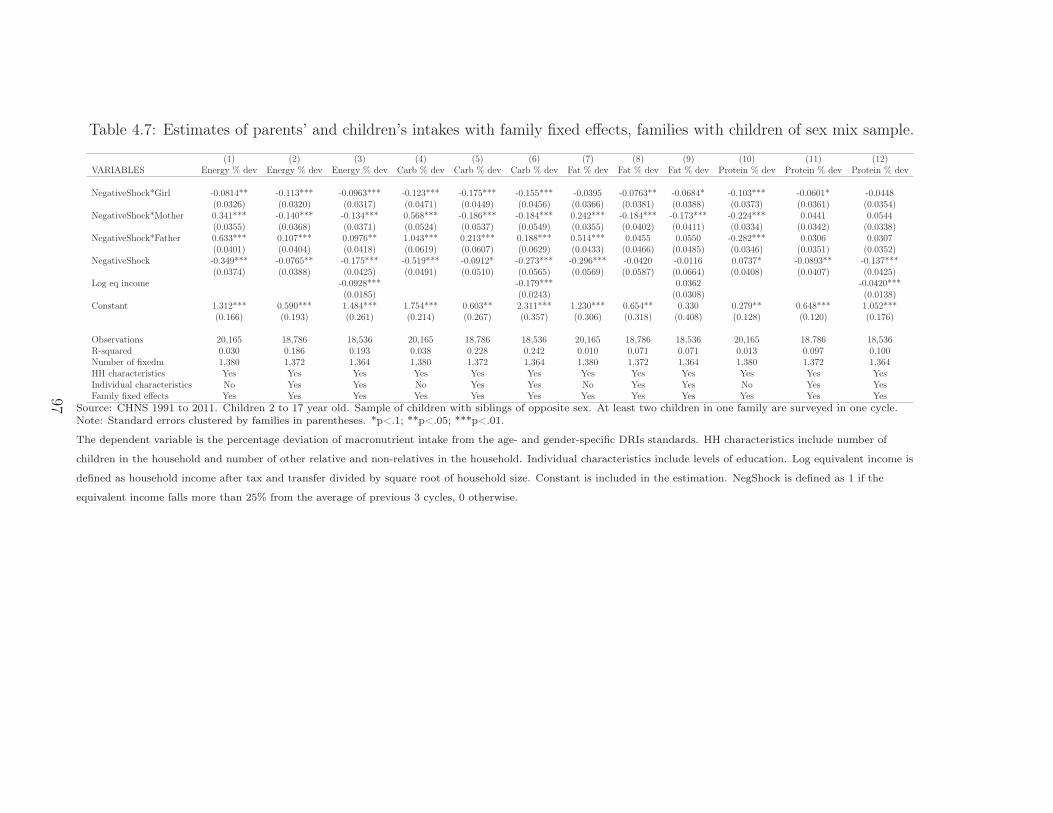
Table 4.7: Estimates of parents’ and children’s intakes with family fixed effects, families with children of sex mix sample.


NegativeShock*Girl -0.0814** -0.113*** -0.0963*** -0.123*** -0.175*** -0.155*** -0.0395 -0.0763** -0.0684* -0.103*** -0.0601* -0.0448(0.0326) (0.0320) (0.0317) (0.0471) (0.0449) (0.0456) (0.0366) (0.0381) (0.0388) (0.0373) (0.0361) (0.0354)

NegativeShock*Mother 0.341*** -0.140*** -0.134*** 0.568*** -0.186*** -0.184*** 0.242*** -0.184*** -0.173*** -0.224*** 0.0441 0.0544(0.0355) (0.0368) (0.0371) (0.0524) (0.0537) (0.0549) (0.0355) (0.0402) (0.0411) (0.0334) (0.0342) (0.0338)

NegativeShock*Father 0.633*** 0.107*** 0.0976** 1.043*** 0.213*** 0.188*** 0.514*** 0.0455 0.0550 -0.282*** 0.0306 0.0307(0.0401) (0.0404) (0.0418) (0.0619) (0.0607) (0.0629) (0.0433) (0.0466) (0.0485) (0.0346) (0.0351) (0.0352)

NegativeShock -0.349*** -0.0765** -0.175*** -0.519*** -0.0912* -0.273*** -0.296*** -0.0420 -0.0116 0.0737* -0.0893** -0.137***(0.0374) (0.0388) (0.0425) (0.0491) (0.0510) (0.0565) (0.0569) (0.0587) (0.0664) (0.0408) (0.0407) (0.0425)

Log eq income -0.0928*** -0.179*** 0.0362 -0.0420***(0.0185) (0.0243) (0.0308) (0.0138)

Constant 1.312*** 0.590*** 1.484*** 1.754*** 0.603** 2.311*** 1.230*** 0.654** 0.330 0.279** 0.648*** 1.052***(0.166) (0.193) (0.261) (0.214) (0.267) (0.357) (0.306) (0.318) (0.408) (0.128) (0.120) (0.176)

Observations 20,165 18,786 18,536 20,165 18,786 18,536 20,165 18,786 18,536 20,165 18,786 18,536R-squared 0.030 0.186 0.193 0.038 0.228 0.242 0.010 0.071 0.071 0.013 0.097 0.100Number of fixedm 1,380 1,372 1,364 1,380 1,372 1,364 1,380 1,372 1,364 1,380 1,372 1,364HH characteristics Yes Yes Yes Yes Yes Yes Yes Yes Yes Yes Yes YesIndividual characteristics No Yes Yes No Yes Yes No Yes Yes No Yes YesFamily fixed effects Yes Yes Yes Yes Yes Yes Yes Yes Yes Yes Yes Yes



children in the household and number of other relative and non-relatives in the household. Individual characteristics include levels of education. Log equivalent income is

defined as household income after tax and transfer divided by square root of household size. Constant is included in the estimation. NegShock is defined as 1 if the

equivalent income falls more than 25% from the average of previous 3 cycles, 0 otherwise.

97

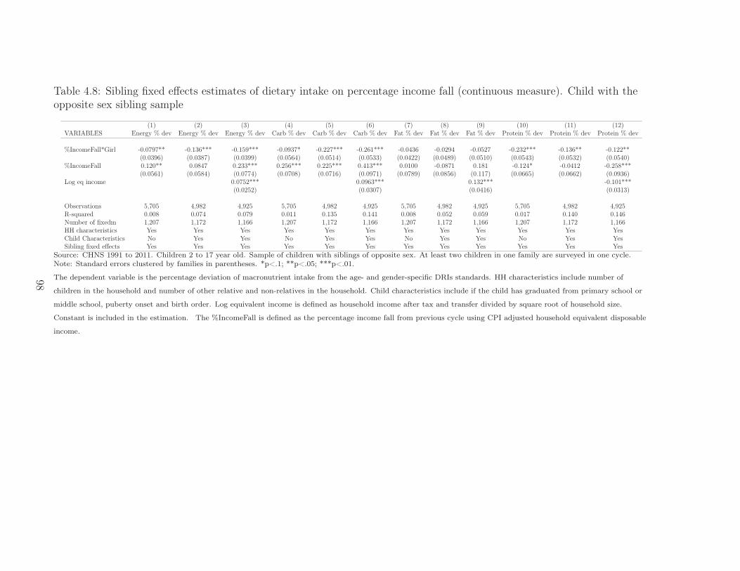
Table 4.8: Sibling fixed effects estimates of dietary intake on percentage income fall (continuous measure). Child with theopposite sex sibling sample


%IncomeFall*Girl -0.0797** -0.136*** -0.159*** -0.0937* -0.227*** -0.261*** -0.0436 -0.0294 -0.0527 -0.232*** -0.136** -0.122**(0.0396) (0.0387) (0.0399) (0.0564) (0.0514) (0.0533) (0.0422) (0.0489) (0.0510) (0.0543) (0.0532) (0.0540)

%IncomeFall 0.120** 0.0847 0.233*** 0.256*** 0.225*** 0.413*** 0.0100 -0.0871 0.181 -0.124* -0.0412 -0.258***(0.0561) (0.0584) (0.0774) (0.0708) (0.0716) (0.0971) (0.0789) (0.0856) (0.117) (0.0665) (0.0662) (0.0936)

Log eq income 0.0752*** 0.0963*** 0.132*** -0.101***(0.0252) (0.0307) (0.0416) (0.0313)






Constant is included in the estimation. The %IncomeFall is defined as the percentage income fall from previous cycle using CPI adjusted household equivalent disposable

income.

98

Table 4.9: Sibling fixed effects estimates of dietary intake on percentage income fall (continuous measure). Adolescents withthe opposite sex sibling sample


%IncomeFall*Girl -0.279*** -0.321*** -0.330*** -0.384*** -0.507*** -0.527*** -0.193** -0.219** -0.239** -0.208*** -0.0690 -0.0495(0.0710) (0.0756) (0.0791) (0.101) (0.105) (0.110) (0.0859) (0.0932) (0.0979) (0.0738) (0.0758) (0.0775)

%IncomeFall 0.0769 0.0954 0.382*** 0.263** 0.288** 0.720*** -0.118 -0.110 0.130 -0.0736 -0.0674 -0.0493(0.0934) (0.0937) (0.134) (0.124) (0.125) (0.169) (0.136) (0.137) (0.206) (0.0811) (0.0772) (0.108)

Log eq income 0.132*** 0.199*** 0.109 0.0122(0.0463) (0.0582) (0.0720) (0.0399)

Observations 2,223 2,188 2,170 2,223 2,188 2,170 2,223 2,188 2,170 2,223 2,188 2,170R-squared 0.020 0.030 0.040 0.028 0.055 0.068 0.017 0.022 0.026 0.026 0.106 0.103Number of fixedm 962 951 946 962 951 946 962 951 946 962 951 946HH characteristics Yes Yes Yes Yes Yes Yes Yes Yes Yes Yes Yes YesChild Characteristics No Yes Yes No Yes Yes No Yes Yes No Yes YesSibling fixed effects Yes Yes Yes Yes Yes Yes Yes Yes Yes Yes Yes Yes





Constant is included in the estimation. The %IncomeFall is defined as the percentage income fall from previous cycle using CPI adjusted household equivalent disposable

income.

99

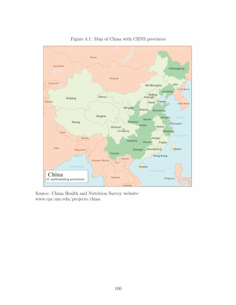
Figure 4.1: Map of China with CHNS provinces

Source: China Health and Nutrition Survey website:www.cpc.unc.edu/projects/china

100

Figure 4.2: Fertility Rate for Rural and Urban China (1973-2010)

Source: The figure is reproduced based on data from Zhang (2017). It is originallycompiled from Peng and Guo (2017) for 1973-1992 data; the 2001 National Fertil-ity and Reproductive Health Survey for 1993-1999; Juan and Qiu (2011) for 2001-2009 data; and the national population censuses for 2000 and 2010 data.

101

Figure 4.3: Outcome variables by gender and single child status

.65

.7.7

5.8

.85

Boy with sib Girl with sib Only boy Only girl

Protein % dev

.4.6

.81

1.2


Fat % dev

.75

.8.8

5.9

.95

1


Energy % dev

.6.8

11.

21.

4


Carb % dev

.34

.36

.38

.4.4

2


Protein % dev1.

11.

21.

31.

41.

51.

6


Fat % dev

1.4

1.5

1.6

1.7


Energy % dev

1.6

1.8

22.

22.

4


Carb % dev

.38

.4.4

2.4

4.4

6.4

8


Protein % dev

.8.9

11.

11.

21.

3


Fat % dev

1.1

1.2

1.3

1.4


Energy % dev

1.2

1.4

1.6

1.8

2


Carb % dev

Note: CHNS 1991 to 2011. Children 2 to 17 year old. Sibling sample and single child sample. %Dev is defined as the per-centage deviation of macronutrient intakes from the age- and gender-specific DRIs standards.

102

Figure 4.4: Independent variables by gender and single child status

.04

.06

.08

.1.1

2


NegativeShock

2.5

2.6

2.7

2.8

2.9


Number of extra hh members

8000

1000

012

000

1400

016

000


Equivalent Income

.5.6

.7.8


Rural residents.2

4.2

6.2

8.3

.32

.34


Primary Schooling

.15

.2.2

5.3

.35


Middle Schooling

Note: CHNS 1991 to 2011. Children 2 to 17 year old. Sibling sample and single child sample. NegShock is defined as 1 ifthe equivalent income falls more than 25% from the average of previous 3 cycles, 0 otherwise. Number of extra hh membersis defined as household size minus two parents minus number of children (e.g. number of grandparents, relatives, and non-relatives). Equivalent income is defined as household income after tax and transfer divided by square root of household size.

103

Figure 4.5: Energy distribution with and without negative income shock

Father159%

Mother130%

Son 97%

Daughter84%

Without NegShock

Father162%

Mother108%

Son 90%

Daughter65%

With NegShock

Source: Author’s calculation. Note: The without income shock is used from the mean energy intakes of the sample. Thewith income shock is calculated using the estimates from Table 4.7 Specification 2. The percentage deviation of energy in-take from DRIs standard is labelled.

104

Chapter 5

Conclusion

In this dissertation, I examine the links between parental economic insecurity and

child development. Economic insecurity does not have a unified measure (Osberg,

2015a). Therefore, I examine three different measures of economic insecurity in my

three essays. First, I use subjective measure, where parents are directly asked if

they worry about having enough money to support their families. The second es-

say uses objective measures of layoff rates and financial loss in the event of layoffs

at the provincial and year level. In the third essay, a 25% income loss from pre-

vious years is used. Economic insecurity examined in this dissertation combines

subjective and objective measures at the individual, household, and provincial

level. By engaging different measures, I provide a multidimensional overview of

the prevalence and the severity of economic insecurity.

To draw causal conclusions, I use two methods in the three essays. The second es-

say uses continuous difference-in-difference methodology. The third essay adopts

sibling fixed effects to control for unobserved heterogeneity in the family. By em-

ploying the three econometric techniques, I hope to provide strong evidence to

infer the causal relationship of parental economic insecurity and the adversity of

child outcomes.

In the dissertation, I investigate the parental economic insecurity and child devel-

opment in both China and Canada. The two countries vary in economic develop-

ment, welfare state, constitutions, cultures, population size, and political attitudes.

I adopt the concept and methodology of economic insecurity and bring them to

Chinese studies. China’s pension, social assistance programs, and employment

insurances are severely underdeveloped, which contributes to a high level of eco-

nomic insecurity. However, economic insecurity is highly understudied in China.

I adapt my focus of the study to the country-specific environment. I provide evi-

dence to China-specific issues (e.g. layoffs and son-favoritism). By doing so, I hope

105

to bridge the studies of two cultures and draw attention to the insecurity in both

countries.

106

References

Abraham, S., Collins, G., & Nordsieck, M. (1971). Relationship of childhoodweight status to morbidity in adults. HSMHA health reports, 86 (3), 273.

Almond, D., Edlund, L., & Milligan, K. (2013). Son preference and the persis-tence of culture: Evidence from south and East Asian immigrants to canada.Population and Development Review , 39 (1), 75–95.

Angrist, J. D., & Pischke, J.-S. (2008). Mostly harmless econometrics: An empiri-cist’s companion. Princeton university press.

Bezirganian, S., & Cohen, P. (1992). Sex differences in the interaction betweentemperament and parenting. Journal of the American Academy of Child &Adolescent Psychiatry , 31 (5), 790–801.

Birch, L. L., & Fisher, J. O. (1998). Development of eating behaviors amongchildren and adolescents. Pediatrics , 101 (Supplement 2), 539–549. Re-trieved from http://pediatrics.aappublications.org/content/101/Supplement_2/539

Blanchflower, D. G., & Oswald, A. J. (1999). Well-being, insecurity and the declineof american job satisfaction. NBER working paper , 7487 .

Blau, D. M. (1999). The effect of income on child development. Review of Eco-nomics and Statistics, 81 (2), 261–276.

Brooks-Gunn, J., & Duncan, G. J. (1997). The effects of poverty on children. Thefuture of children, 55–71.

Burkhauser, R. V., & Cawley, J. (2008). Beyond bmi: The value of more accuratemeasures of fatness and obesity in social science research. Journal of healtheconomics, 27 (2), 519–529.

Burton, P., & Phipps, S. (2009). Economic costs of caring for children with disabil-ities in canada. Canadian Public Policy , 35 (3), 269–290.

Burton, P., Phipps, S., & Woolley, F. (2007). Inequality within the householdreconsidered. In S. Jenkins & J. Micklewright (Eds.), Inequality and povertyreexamined (p. 103-125). Oxford: Oxford University Press.

Cai, H., Li, H., Park, A., & Zhou, L.-A. (2013). Family ties and organizationaldesign: Evidence from chinese private firms. Review of Economics and Statis-tics , 95 (3), 850–867.

Cartwright-Hatton, S., McNicol, K., & Doubleday, E. (2006). Anxiety in a ne-glected population: Prevalence of anxiety disorders in pre-adolescent chil-dren. Clinical psychology review , 26 (7), 817–833.

Chang, K.-c. (1977). Food in chinese culture: Anthropological and historical per-spectives. Yale University Press.

Chartrand, T. L., & Bargh, J. A. (1999). The chameleon effect: the perception–behavior link and social interaction. Journal of personality and social psy-chology , 76 (6), 893.

107

Chee, B. W. (2000). Eating snacks and biting pressure: only children in beijing.Feeding China’s little emperors: food, children, and social change, 48–70.

Chen, K., Fortin, N., & Phipps, S. (2015). Young in class: implications for inatten-tive/hyperactive behaviour of canadian boys and girls. Canadian Journal ofEconomics/Revue canadienne d’économique, 48 (5), 1601–1634.

Chen, Y., Li, H., & Meng, L. (2013). Prenatal sex selection and missing girls inChina: Evidence from the diffusion of diagnostic ultrasound. Journal of Hu-man Resources , 48 (1), 36–70.

China Health and Nutrition Survey. (2017). Retrieved from http://www.cpc.unc.edu/projects/china (Accessed: April 16, 2017)

Clark, A., & Grey, A. (1997). Is job insecurity on the increase in oecd countries.DEELSA, OECD, mimeografado, Março.

Cole, T. J., Bellizzi, M. C., Flegal, K. M., & Dietz, W. H. (2000). Establishing astandard definition for child overweight and obesity worldwide: Internationalsurvey. Bmj , 320 (7244), 1240.

Cole, T. J., & Green, P. J. (1992). Smoothing reference centile curves: The lmsmethod and penalized likelihood. Statistics in medicine, 11 (10), 1305–1319.

Cui, Z., & Dibley, M. J. (2012). Trends in dietary energy, fat, carbohydrate andprotein intake in chinese children and adolescents from 1991 to 2009. BritishJournal of Nutrition, 108 (7), 1292–1299. doi: 10.1017/S0007114511006891

Cunha, F., & Heckman, J. J. (2010). Investing in our young people (Tech. Rep.).National Bureau of Economic Research.

Dahl, G. B., & Lochner, L. (2012). The impact of family income on child achieve-ment: Evidence from the earned income tax credit. The American EconomicReview , 102 (5), 1927–1956.

Dallman, M. F., Pecoraro, N., Akana, S. F., La Fleur, S. E., Gomez, F., Housh-yar, H., . . . Manalo, S. (2003). Chronic stress and obesity: A new view of“comfort food”. Proceedings of the National Academy of Sciences, 100 (20),11696–11701.

Das Gupta, M., Ebenstein, A. Y., & Sharygin, E. J. (2010). China’s marriagemarket and upcoming challenges for elderly men.

Dasgupta, P. (1995). An inquiry into well-being and destitution. Oxford UniversityPress on Demand.

Dawson, D. A. (1991). Family structure and children’s health and well-being: Datafrom the 1988 national health interview survey on child health. Journal ofMarriage and the Family , 573–584.

Demarest, J., & Allen, R. (2000). Body image: Gender, ethnic, and age differences.The Journal of social psychology , 140 (4), 465–472.

Deurenberg, P., Deurenberg-Yap, M., & Guricci, S. (2002). Asians are differentfrom caucasians and from each other in their body mass index/body fat percent relationship. Obesity reviews, 3 (3), 141–146.

Di Tella, R., MacCulloch, R. J., & Oswald, A. J. (2001). Preferences over infla-tion and unemployment: Evidence from surveys of happiness. The Americaneconomic review , 91 (1), 335–341.

108

Di Tella, R., MacCulloch, R. J., & Oswald, A. J. (2003). The macroeconomics ofhappiness. Review of Economics and Statistics, 85 (4), 809–827.

Dorfman, M. C., Holzmann, R., O’keefe, P., Wang, D., Sin, Y., & Hinz, R. (2013).China’s pension system: A vision. World Bank Publications.

Duflo, E. (2000). Child health and household resources in south africa: evidencefrom the old age pension program. The American Economic Review , 90 (2),393–398.

Ebenstein, A. (2010). The “missing girls” of China and the unintended conse-quences of the one child policy. Journal of Human Resources, 45 (1), 87–115.

Essex, M. J., Klein, M. H., Cho, E., & Kraemer, H. C. (2003). Exposure to ma-ternal depression and marital conflict: Gender differences in children’s latermental health symptoms. Journal of the American Academy of Child & Ado-lescent Psychiatry , 42 (6), 728–737.

Friedman, M. A., & Brownell, K. D. (1995). Psychological correlates of obesity:Moving to the next research generation. Psychological bulletin, 117 (1), 3.

Furnham, A., Badmin, N., & Sneade, I. (2002). Body image dissatisfaction: Gen-der differences in eating attitudes, self-esteem, and reasons for exercise. TheJournal of psychology , 136 (6), 581–596.

Gershoff, E. T., Aber, J. L., Raver, C. C., & Lennon, M. C. (2007). Income is notenough: Incorporating material hardship into models of income associationswith parenting and child development. Child development , 78 (1), 70–95.

Giles, J., Park, A., & Cai, F. (2006). How has economic restructuring affectedChina’s urban workers? The China Quarterly , 185 , 61–95.

Greeno, C. G., & Wing, R. R. (1994). Stress-induced eating. Psychological bulletin,115 (3), 444.

Guo, S. S., Roche, A. F., Chumlea, W. C., Gardner, J. D., & Siervogel, R. M.(1994). The predictive value of childhood body mass index values for over-weight at age 35 y. The American journal of clinical nutrition, 59 (4), 810–819.

Hacker, J. S., Huber, G. A., Nichols, A., Rehm, P., Schlesinger, M., Valletta, R., &Craig, S. (2014). The economic security index: A new measure for researchand policy analysis. Review of Income and Wealth, 60 , S5–S32. Retrievedfrom http://dx.doi.org/10.1111/roiw.12053 doi: 10.1111/roiw.12053

Hacker, J. S., Huber, G. A., Rehm, P., Schlesinger, M., & Valletta, R. (2010). Eco-nomic security at risk. The Rockefeller Foundation.

Haddad, L., & Hoddinott, J. (1994). Women’s income and boy-girl anthropo-metric status in the côte d’ivoire. World Development , 22 (4), 543 - 553.Retrieved from http://www.sciencedirect.com/science/article/pii/0305750X94901104 doi: http://dx.doi.org/10.1016/0305-750X(94)90110-4

Hanushek, E. A. (1992). The trade-off between child quantity and quality. Journalof political economy , 100 (1), 84–117.

Heckman, J. J. (2000). Policies to foster human capital. Research in economics,54 (1), 3–56.

Heckman, J. J. (2007). The economics, technology, and neuroscience of human109

capability formation. Proceedings of the national Academy of Sciences,104 (33), 13250–13255.

Heckman, J. J. (2011). The economics of inequality: The value of early childhoodeducation. American Educator , 35 (1), 31.

Helliwell, J. F., & Huang, H. (2014). New measures of the costs of unemployment:Evidence from the subjective well-being of 3.3 million americans. EconomicInquiry , 52 (4), 1485–1502.

Hesketh, T., Lu, L., & Xing, Z. W. (2005). The effect of China’s one-child familypolicy after 25 years. Mass Medical Soc.

Jing, J. (2000). Feeding China’s little emperors: Food, children, and social change.Stanford University Press.

Johansson, S., & Nygren, O. (1991). The missing girls of China: A new demo-graphic account. The Population and Development Review , 35–51.

Juan, H., & Qiu, C. (2011). A comparative analysis of the fertility of the urbanand rural areas in China since 2000. South China Population, 5 , 27–33.

Kavey, R.-E. W., Daniels, S. R., Lauer, R. M., Atkins, D. L., Hayman, L. L., &Taubert, K. (2003). American heart association guidelines for primary pre-vention of atherosclerotic cardiovascular disease beginning in childhood. Cir-culation, 107 (11), 1562–1566.

Ko, G. T., Chan, J. C., Cockram, C. S., & Woo, J. (1999). Prediction of hyper-tension, diabetes, dyslipidaemia or albuminuria using simple anthropometricindexes in hong kong chinese. International journal of obesity , 23 (11), 1136–1142.

Kong, W., & Phipps, S. (2016). Parental economic insecurity and children’s non-cognitive skills: A panel study of 2 to 5 year-olds in canada.. (Paper pre-pared for the 34th IARIW General Conference Dresden, Germany, August21-27, 2016)

Kuczmarski, R. J., Ogden, C. L., Grummer-Strawn, L. M., Flegal, K. M., Guo,S. S., Wei, R., . . . Johnson, C. L. (2000). Cdc growth charts: United states.Advance data(314), 1–27.

Köster, E. P., & Mojet, J. (2015). From mood to food and from food to mood:A psychological perspective on the measurement of food-related emotionsin consumer research. Food Research International , 76 , 180 - 191. Re-trieved from http://www.sciencedirect.com/science/article/pii/S096399691500157X (Food, emotions and food choice)

Larson, J. H., Wilson, S. M., & Beley, R. (1994). The impact of job insecurity onmarital and family relationships. Family Relations , 138–143.

Lee, H. Y. (2000). Xiagang, the chinese style of laying off workers. Asian Survey ,40 (6), 914–937.

Lefebvre, P., Merrigan, P., & Verstraete, M. (2006). Impact of early childhood careand education on children’s preschool cognitive development: Canadian resultsfrom a large quasi-experiment (Tech. Rep.). CIRPEE.

Levy, D. M., & Duncan, G. (2000, April). Using Sibling Samples to Assess theEffect of Childhood Family Income on Completed Schooling (JCPR Working

110

Papers No. 168). Northwestern University/University of Chicago Joint Cen-ter for Poverty Research. Retrieved from https://ideas.repec.org/p/wop/jopovw/168.html

Lin, J. Y., Cai, F., & Li, Z. (1998). Competition, policy burdens, and state-ownedenterprise reform. The American Economic Review , 88 (2), 422–427.

Lise, J., & Seitz, S. (2011). Consumption inequality and intra-household alloca-tions. The Review of Economic Studies, 78 (1), 328–355.

Liu, C., Xie, B., Chou, C.-P., Koprowski, C., Zhou, D., Palmer, P., . . . others(2007). Perceived stress, depression and food consumption frequency in thecollege students of China seven cities. Physiology & behavior , 92 (4), 748–754.

Lundberg, S. J., Pollak, R. A., & Wales, T. J. (1997). Do husbands and wives pooltheir resources? evidence from the united kingdom child benefit. Journal ofHuman resources , 463–480.

Lupien, S. J., McEwen, B. S., Gunnar, M. R., & Heim, C. (2009). Effects of stressthroughout the lifespan on the brain, behaviour and cognition. Nature re-views. Neuroscience, 10 (6), 434.

Luxembourg Income Study. (2017). Retrieved from http://www.lisdatacenter.org (Accessed: April 16, 2017)

Macht, M. (2008). How emotions affect eating: A five-way model. Appetite, 50 (1),1 - 11. Retrieved from http://www.sciencedirect.com/science/article/pii/S0195666307003236 doi: https://doi.org/10.1016/j.appet.2007.07.002

Mayer, S. E. (1997). What money can’t buy: Family income and children’s lifechances. Harvard University Press.

Millward, D. J., & Jackson, A. A. (2003). Protein/energy ratios of current dietsin developed and developing countries compared with a safe protein/energyratio: implications for recommended protein and amino acid intakes. Publichealth nutrition, 7 (03), 387–405.

Mokha, J. S., Srinivasan, S. R., DasMahapatra, P., Fernandez, C., Chen, W., Xu,J., & Berenson, G. S. (2010). Utility of waist-to-height ratio in assessing thestatus of central obesity and related cardiometabolic risk profile among nor-mal weight and overweight/obese children: The bogalusa heart study. BMCpediatrics , 10 (1), 73.

Offer, A., Pechey, R., & Ulijaszek, S. (2010). Obesity under affluence varies bywelfare regimes: The effect of fast food, insecurity, and inequality. Eco-nomics & Human Biology , 8 (3), 297 - 308. Retrieved from http://www.sciencedirect.com/science/article/pii/S1570677X10000663 doi:https://doi.org/10.1016/j.ehb.2010.07.002

Onis, M. (2006). Who child growth standards based on length/height, weight andage. Acta paediatrica, 95 (S450), 76–85.

Onis, M. d., Onyango, A. W., Borghi, E., Siyam, A., Nishida, C., & Siekmann, J.(2007a). Development of a who growth reference for school-aged children andadolescents. Bulletin of the World health Organization, 85 (9), 660–667.

Onis, M. d., Onyango, A. W., Borghi, E., Siyam, A., Nishida, C., & Siekmann, J.111

(2007b). Development of a who growth reference for school-aged children andadolescents. Bulletin of the World health Organization, 85 (9), 660–667.

Oreopoulos, P., Page, M. E., & Stevens, A. H. (2006). The intergenerational effectsof compulsory schooling. Journal of Labor Economics , 24 (4), 729–760.

Osberg, L. (1998, October). Economic Insecurity. SPRC Discussion Paper, So-cial Policy Research Centre, University of New South Wales, Sydney, Aus-tralia(No. 88).

Osberg, L. (2000). Poverty in canada and the united states: Measurement, trends,and implications. The Canadian Journal of Economics/Revue Canadienned’Economique, 33 (4), 847–877.

Osberg, L. (2015a). How should one measure economic insecurity? OECD Statis-tics Working Papers , 2015 (1), 0_1.

Osberg, L. (2015b). The hunger of old women in rural tanzania: Can subjectivedata improve poverty measurement? Review of Income and Wealth, 61 (4),723–738.

Osberg, L., & Sharpe, A. (2009a). Measuring economic security in insecure times:New perspectives, new events, and the index of economic well-being (Tech.Rep.). Centre for the Study of Living Standards Ottawa.

Osberg, L., & Sharpe, A. (2009b). New estimates of the index of economic well-being for selected oecd countries, 1980-2007. Centre for the Study of LivingStandards.

Peng, X. (1991). Demographic transition in China: fertility trends since the 1950s.Oxford: Clarendon Press.

Peng, X., & Guo, Z. (2000). The changing population of China. Blackwell Publish-ers.

Phipps, S., & Burton, P. (1995). Sharing within families: implications for themeasurement of poverty among individuals in canada. Canadian Journal ofEconomics , 177–204.

Phipps, S., Burton, P., & Osberg, L. (2001). Time as a source of inequality withinmarriage: are husbands more satisfied with time for themselves than wives?Feminist Economics, 7 (2), 1–21.

Popkin, B. M., Du, S., Zhai, F., & Zhang, B. (2010). Cohort profile: The ChinaHealth and Nutrition Survey—monitoring and understanding socio-economicand health change in china, 1989–2011. International journal of epidemiol-ogy , 39 (6), 1435–1440.

Popkin, B. M., Lu, B., & Zhai, F. (2002). Understanding the nutrition transition:measuring rapid dietary changes in transitional countries. Public health nutri-tion, 5 (6a), 947–953.

Qvortrup, J., Bardy, M., Sgritta, G., & Wintersberger, H. (1994). Childhood mat-ters: Social theory, practice and politics. Avebury.

Rohde, N., Tang, K., & Osberg, L. (2017). The self-reinforcing dynamics of eco-nomic insecurity and obesity. Applied Economics, 49 (17), 1668–1678.

Rohde, N., Tang, K. K., Osberg, L., & Rao, P. (2016). The effect of economic inse-curity on mental health: Recent evidence from australian panel data. Social

112

Science & Medicine, 151 , 250–258.Sawyer, S. M., Afifi, R. A., Bearinger, L. H., Blakemore, S.-J., Dick, B., Ezeh,

A. C., & Patton, G. C. (2012). Adolescence: a foundation for future health.The Lancet , 379 (9826), 1630–1640.

Schneider, H. J., Friedrich, N., Klotsche, J., Pieper, L., Nauck, M., John, U., . . .others (2010). The predictive value of different measures of obesity for inci-dent cardiovascular events and mortality. The Journal of Clinical Endocrinol-ogy & Metabolism, 95 (4), 1777–1785.

Smith, T. G. (2009). Reconciling psychology with economics: Obesity, behavioralbiology, and rational overeating. Journal of Bioeconomics, 11 (3), 249–282.Retrieved from http://dx.doi.org/10.1007/s10818-009-9067-8 doi:10.1007/s10818-009-9067-8

Smith, T. G., Stoddard, C., & Barnes, M. G. (2009). Why the poor get fat:weight gain and economic insecurity. In Forum for health economics & pol-icy (Vol. 12).

Sørensen, T. L., & Sonne-Holm, S. (1988). Risk in childhood of development of se-vere adult obesity: Retrospective, population-based case-cohort study. Amer-ican journal of epidemiology , 127 (1), 104–113.

Staudigel, M. (2016). A soft pillow for hard times? economic insecurity, food in-take and body weight in russia. Journal of Health Economics, 50 , 198 - 212.Retrieved from http://www.sciencedirect.com/science/article/pii/S0167629616301928 doi: https://doi.org/10.1016/j.jhealeco.2016.09.001

Trumbo, P., Schlicker, S., Yates, A. A., & Poos, M. (2002). Dietary reference in-takes for energy, carbohydrate, fiber, fat, fatty acids, cholesterol, protein andamino acids. Journal of the American Dietetic Association, 102 (11), 1621–1630.

Tsutsumi, A., Kayaba, K., Theorell, T., & Siegrist, J. (2001). Association betweenjob stress and depression among japanese employees threatened by job loss ina comparison between two complementary job-stress models. Scandinavianjournal of work, environment & health, 146–153.

Watson, B., Osberg, L., & Phipps, S. (2016). Economic insecurity and the weightgain of canadian adults: A natural experiment approach. Canadian Pub-lic Policy , 42 (2), 115-131. Retrieved from https://doi.org/10.3138/cpp.2015-064 doi: 10.3138/cpp.2015-064

World Health Organization. (2000). The Asia-Pacific perspective: redefining obesityand its treatment. Sydney: Health Communications Australia.

World Health Organization. (2006). Who child growth standards: length/height forage, weight-for-age, weight-for-length, weight-for-height and body mass index-for-age, methods and development. World Health Organization.

World Health Organization. (2017). Retrieved from http://www.who.int/maternal_child_adolescent/topics/adolescence/dev/en/ (Accessed:April 16, 2017)

Yan, S., Li, J., Li, S., Zhang, B., Du, S., Gordon-Larsen, P., . . . Popkin, B. (2012).The expanding burden of cardiometabolic risk in China: The China health

113

and nutrition survey. Obesity Reviews, 13 (9), 810–821.Yan, W., Bingxian, H., Hua, Y., Jianghong, D., Jun, C., Dongliang, G., . . . others

(2007). Waist-to-height ratio is an accurate and easier index for evaluatingobesity in children and adolescents. Obesity , 15 (3), 748–752.

Zhang, J. (2017). The evolution of China’s one-child policy and its effects on fam-ily outcomes. Journal of Economic Perspectives, 31 (1).

Zhou, W. (2014). Brothers, household financial markets and savings rate in China.Journal of Development Economics, 111 , 34–47.

Zhu, M., J, F., L, L., C, G., F, X., G, L., . . . S., C. (2013). Epidemiologic study oncurrent pubertal development in chinese school-aged children. Zhejiang DaXue Xue Bao Yi Xue Ban, 4 (42), 396-402.

114

Appendix

Children’s well-being outcomes The three indices for children’s well-being

outcomes are derived from multiple questions answered by PMKs. The questions

and answers follow the same format: “Using the answers never or not true, some-

times or somewhat true, or often or very true, how often would you say that this

child. . . ” For all of the questions, never or not true is assigned 0, sometimes or

somewhat true is 1, and often or very true is 2. Then the score from each ques-

tion is combined under the same index. Here is the list of questions asked for hy-

peractivity/inattention score, emotional disorder/anxiety score and conduct disor-

der/physical aggression score:

Hyperactivity - Inattention score (12-point scale) is derived from the following six

questions:

1. . . . can’t sit still or is restless?

2. . . . is easily distracted, has trouble sticking to any activity?

3. . . . can’t concentrate, can’t pay attention for long?

4. . . . cannot settle on anything for more than a few moments?

5. . . . has difficulty waiting for his turn in games or groups?

6. . . . is inattentive?

Emotional Disorder-Anxiety Score (12-point scale) is derived from the following six

questions:

1. . . . seems to be unhappy or sad?

2. . . . is not as happy as other children?

3. . . . is too fearful or nervous?

4. . . . is worried?

5. . . . is nervous, high strung or tense?

6. . . . has trouble enjoying him/herself?115

Parenting style

Consistent parenting style score (20-point scale) is derived from the questions be-

low. The answers to these questions ranging from 0 (never) to 4 (all the time).

The values of last three questions are reversed for the calculation.

1. When you give this child a command or order to do something, what propor-

tion of the time do you make sure that he does it?

2. If you tell this child he will get punished if he doesn’t stop doing something,

and he keeps doing it, how often will you punish him?

3. How often does this child get away with things for which you feel he should

have been punished?

4. How often is this child able to get out of a punishment when he really sets

his mind to it?

5. How often when you discipline this child, does he ignore the punishment?

Positive interaction score (20-point scale) are derived from the questions below.

These questions take the value 0 if never, 1 if about once a week or less, 2 if a few

times a week, 3 one or two times a day, and 4 many times each day.

1. 1. How often do you praise this child, by saying something like ’Good for

you!’ or ’What a nice thing you did!’ or ’That’s good going!’?

2. How often do you and this child talk or play with each other, focusing atten-

tion on each other for five minutes or more, just for fun?

3. How often do you and this child laugh together?

4. How often do you do something special with this child that he enjoys?

5. How often do you play sports, hobbies or games with this child?

Ineffective parenting style score ranges from 0 to 28. It is derived from the follow-

ing seven questions with the same calculation as above.

1. How often do you get annoyed with this child for saying or doing something

he is not supposed to?116

2. Of all the times that you talk to this child about his behaviour, what propor-

tion is praise? (reversed)

3. Of all the times that you talk to this child about his behaviour, what propor-

tion is disapproval?

4. How often do you get angry when you punish this child?

5. How often do you think that the kind of punishment you give this child de-

pends on your mood?

6. How often do you feel you are having problems managing this child in gen-

eral?

7. How often do you have to discipline this child repeatedly for the same thing?

Irrational parenting style score is on 16-point scale. Parents are asked to answer

the questions from 0 “Never” to 4 “Always”. The four questions are asked as fol-

lowing: “Please tell me how often you, as his parent, do each of the following when

this child breaks the rules or does things that he is not supposed to:”

1. ...raise your voice, scold or yell at him?

2. ...calmly discuss the problem? (reversed)

3. ...use physical punishment?

4. ...describe alternative ways of behaving that are acceptable? (reversed)

117

State-owned units: various enterprises, institutions, and government administra-

tive organizations at various levels, social organizations, etc., with state ownership

of production means.

Urban collective owned units: various enterprises and institutions with collec-

tive ownership of production means, including various rural economic organizations

engaging in agriculture, forestry, animal husbandry and fishery, enterprises, and

institutions run by townships and villages. Or run by cities, countries, towns, and

neighbourhood committees.

Other Ownership Units:: jointly owned units, share-holding units, foreign-

funded units, overseas Chinese from Hong Kong, Macao, and Taiwan-funded units,

etc.

Laid-off workers: due to the production or operational difficulties of the state-

sector enterprises, employees leave the job involuntarily, and do not work for other

jobs in the same enterprise. They still remain the labour relation with the original

enterprises (National Bureau of Labour & National Bureau of Statistics of China,

1997)

118

three essays on economic insecurity and child …

Documents