three essays on the determinants of corporate cash...

THREE ESSAYS ON THE DETERMINANTS

OF CORPORATE CASH HOLDINGS

by

ANNA-LEIGH STONE

BENTON E. GUP, COMMITTEE CHAIR

DOUGLAS O. COOK

WILLIAM E. JACKSON, III

JUNSOO LEE

JAMES A. LIGON

A DISSERTATION

Submitted in partial fulfillment of the requirements

for the degree of Doctor of Philosophy

in the Department of Economics,

Finance, and Legal Studies

in the Graduate School of

the University of Alabama

TUSCALOOSA, ALABAMA

2015

Copyright Anna-Leigh Stone 2015

ALL RIGHTS RESERVED

ii

ABSTRACT

This dissertation is composed of three essays that investigate three external determinants

of corporate cash holdings: interest rates, business cycles, and unlimited FDIC insurance

guarantees.

In the first essay, theories of the relationship between interest rates and cash holdings

are empirically tested. Based on economic theory, corporate cash holdings should have moved

inversely with these interest rate swings. Using two measures of cash holdings and a random

effects threshold model, we examine this relationship over the past four decades and show that

the expected negative relationship does not exist. Furthermore, the established motives for cash

holdings do not explain these results. Using a quantile regression, we show that a positive

relationship between cash holdings and interest rates primarily exists among firms in lower

quantiles of cash holdings, demonstrating that firms with below average amounts of cash

holdings are driving the results.

In the second essay, the relationship between cash holdings and business cycles is

examined between 1976 and 2012, with a primary emphasis on how cash holdings vary during

recessions. Findings confirm that cash holdings do vary over the business cycle. Upon further

examination, corporate cash holdings initially decline during recessions but increase to levels at

or above pre-crisis levels. In addition, cash holdings appear to increase around the National

Bureau of Economic Research’s announcements of recessions. Therefore, we do not find

iii

evidence of the precautionary motive for cash holdings during recessions but we do find

evidence of an announcement effect for cash holdings.

The third essay examines the unlimited FDIC insurance provisions on noninterest-bearing

transaction accounts provided by the Transaction Account Guarantee Program and Section 343

of the Dodd-Frank Wall Street Reform and Consumer Protection Act. The paper documents an

increase in the funds held in the accounts. Because corporations are known to hold the majority

of these accounts, attention is paid to the potential increase in corporate cash holdings. Using

both time series and panel data techniques, I document an increase in corporate cash holdings

during this time, however, the increase is primarily explained by the uncertainty surrounding the

most recent recession.

iv

DEDICATION

This dissertation is dedicated to my parents, Lyle and Teresa, and my grandparents

without whose love and encouragement I would have never made it this far. It is also dedicated

to Billy Hankins, without whose love, unwavering support, and hours of proofreading I would

never have finished this dissertation. Finally, this dissertation is dedicated in memory of Dr.

Billy Helms who saw promise in a student who did not even see it in herself.

v

LIST OF ABBREVIATIONS, ACRONYMS, AND SYMBOLS

$ American Dollar

= Equal to

> Greater Than

+ In Addition to

< Less Than

≤ Less Than or Equal to

% Percent

AFP Association for Financial Professionals

BIC Bayesian Information Criterion

CBO Congressional Budget Office

CEO Chief Executive Officer

CFO Chief Financial Officer

DB Defined Benefit

FDIC Federal Deposit Insurance Corporation

FE Fixed Effects

FINREG Dodd-Frank Wall Street Reform and Consumer Protection Act

FRED Federal Reserve Economic Data

GDP Gross Domestic Product

vi

GIM Gompers, Ishii, and Metrick

GSE Government-Sponsored Enterprise

HIA Homeland Investment Act

IPO Initial Public Offering

N Number of Observations

NBER National Bureau of Economic Research

OECD Organisation for Economic Co-operation and Development

OLS Ordinary Least Squares

P-value Percentage chance that an estimated effect exists even if, in reality, the

effect does not exist

POLS Pooled Ordinary Least Squares

QMLE Quasi-Maximum Likelihood Estimation

R2

R-squared

R&D Research and Development

S&P Standard & Poor’s

SIC Standard Incorporation Code

SSR Sum of Squared Residuals

T-Bill Treasury Bill

TAG Transaction Account Guarantee

TLG Temporary Liquidity Guarantee

U.S. United States of America

vii

ACKNOWLEDGMENTS

I wish to thank my dissertation chair, Dr. Benton E. Gup, for all the guidance that he has

given me over the years. I would also like to thank all of my committee members, Dr. James

Ligon, Dr. Douglas Cook, Dr. Junsoo Lee, and Dr. William E. Jackson, III, for invaluable

comments and support for both my dissertation and academic pursuits. I would like to thank

several others who have helped with individual essays: Jeffrey Wooldridge, Frederiek

Schoubben, Kevin Roth and Jeff Glenzer of the Association for Financial Executives, and

William B. Hankins, III.

Finally, I would like to thank the Culverhouse College of Commerce and Business

Administration, the Department of Economics, Finance and Legal Studies, the University of

Alabama Graduate School, and the Graduate Student Association for generous financial support,

without which this dissertation would not have been possible.

.

viii

TABLE OF CONTENTS

ABSTRACT ................................................................................................................................... ii

DEDICATION .............................................................................................................................. iv

LIST OF ABBREVIATIONS, ACRONYMS, AND SYMBOLS .................................................v

ACKNOWLEDGMENTS ........................................................................................................... vii

LIST OF TABLES ........................................................................................................................ xi

LIST OF FIGURES .................................................................................................................... xiii

INTRODUCTION ..........................................................................................................................1

CORPORATE CASH HOLDINGS AND INTEREST RATES: 1970-2011 ..................................3

1. Introduction ............................................................................................................................3

2. Literature Review ...................................................................................................................7

3. Hypotheses ...........................................................................................................................10

4. Data ......................................................................................................................................11

5. Econometric Model ..............................................................................................................18

6. Estimation Results and Interpretations .................................................................................23

6.1 Two Threshold Model.....................................................................................................24

6.2 Three Threshold Model...................................................................................................27

7. Tests for the Non-Negative Relationship ..............................................................................30

7.1 Tax-Based Explanation ...................................................................................................31

7.2 Sources of Cash Flow .....................................................................................................32

7.3 Pension Fund Contributions ............................................................................................36

7.4 Zero-Leverage Firms ......................................................................................................39

ix

7.5 Constrained and Unconstrained Firms ............................................................................42

7.6 Alternative Explanations .................................................................................................45

8. Quantile Regression ..............................................................................................................48

9. Conclusion ............................................................................................................................52

References ...................................................................................................................................54

Appendix .....................................................................................................................................57

DO BUSINESS CYCLES INFLUENCE CORPORATE CASH HOLDINGS? ...........................64

1. Introduction ..........................................................................................................................64

2. Literature Review .................................................................................................................68

3. NBER Recessions ................................................................................................................72

4. Data ......................................................................................................................................74

4.1 Data Sets and Corporate Control Variables ....................................................................74

4.2 Variables to Capture Business Cycles ............................................................................76

4.2.1 Macroeconomic Variables .......................................................................................76

4.2.2 Dummy Variables for Recessions and Announced Recessions ...............................78

4.3 Summary Statistics .........................................................................................................81

5. Econometric Models .............................................................................................................84

6. Results and Discussions ........................................................................................................89

6.1 Results with Common Macroeconomic Variables ........................................................89

6.2 Results with Recession Indicators .................................................................................92

6.3 Estimation with Announced Recession Indicator ..........................................................95

6.4 First Quarter Announced Recession ...............................................................................98

7. Constrained and Unconstrained Firms ...............................................................................101

7.1 Results for Constrained and Unconstrained Firms .......................................................102

8. Conclusion .........................................................................................................................106

x

References .................................................................................................................................108

Appendix ...................................................................................................................................111

AN EXAMINATION OF UNILIMITED FDIC INSURANCE AND THE EFFECT ON

CORPORATE CASH HOLDINGS .............................................................................................115

1. Introduction ........................................................................................................................115

2. FDIC Insurance ..................................................................................................................121

2.1 Noninterest-Bearing Accounts ......................................................................................121

2.2 Bank Participation .........................................................................................................125

2.3 Repeal of Regulation Q .................................................................................................134

2.4 Expiration of the Unlimited Insurance ..........................................................................135

3. Corporate Cash Holdings ...................................................................................................136

4. Literature Review and Hypotheses.....................................................................................141

4.1 Literature Review..........................................................................................................141

4.2 Hypotheses ....................................................................................................................143

5. Data ....................................................................................................................................144

6. Econometric Models and Empirical Results ......................................................................147

6.1 Difference-in-Differences ............................................................................................147

6.2 Structural Breaks in Noninterest-Bearing Accounts and Corporate Cash Holdings ....153

6.3 Regression Analysis .....................................................................................................157

7. Conclusion .................................................................................................................................... 161

References .................................................................................................................................163

Appendix ...................................................................................................................................166

CONCLUSION ...........................................................................................................................170

xi

LIST OF TABLES

1.1 Summary Statistics for All, Mature, and Growth Firms ..........................................................16

1.2 Threshold and Interest Rate Statistics ......................................................................................18

1.3 Cash Holdings and Interest Rates ............................................................................................21

1.4 Cash Holdings and Interest Rates with Two Thresholds .........................................................25

1.5 Cash Holdings and Interest Rates with Three Thresholds .......................................................28

1.6 Tax-Based Explanation ............................................................................................................33

1.7 Cash Flow Theory ....................................................................................................................35

1.8 Pension Fund Contributions ....................................................................................................38

1.9 Excluding Zero-Leverage Firms ..............................................................................................40

1.10 Constrained and Unconstrained Firm Summary Statistics ....................................................43

1.11 Constrained and Unconstrained Firms Three Threshold Model ............................................44

1.12 Quantile Regression ...............................................................................................................50

A.1.1 Cash Holdings and Interest Rates with One Threshold .......................................................57

A.1.2 Three Threshold Tax-Based Explanation ...........................................................................59

A.1.3 Mandatory Pension Fund Expense .......................................................................................60

A.1.4 Cash Holdings of Zero-Leverage Firms ...............................................................................61

A.1.5 Constrained and Unconstrained Firms with Two Thresholds ..............................................63

2.1 Recession Dates and Announcement Dates .............................................................................73

2.2 Summary Statistics for All, Mature, and Growth Firms ..........................................................82

xii

2.3 Macroeconomic Summary Statistics........................................................................................84

2.4 Comparisons of Models ...........................................................................................................87

2.5 Macroeconomic Indicators and Cash Holdings .......................................................................90

2.6 Recessions and Cash Holdings ................................................................................................93

2.7 Announced Recessions and Cash Holdings .............................................................................96

2.8 First Quarter of an Announced Recession and Cash Holdings ................................................99

2.9 Business Cycles and Cash Holdings for Constrained and Unconstrained Firms ...................103

A.2.1 Variable Descriptions .........................................................................................................111

A.2.2 First Whole Quarter of an Announced Recession Results .................................................112

A.2.3 Recession Indicator Using Whole Quarters and Cash Holdings ........................................113

3.1 Noninterest-Bearing Accounts Over Time ............................................................................124

3.2 Statistics on Banks Participating in the Transaction Account Guarantee Program by Size ..127

3.3 Noninterest-Bearing Accounts Based on Participation in the TAG Program ........................129

3.4 Capital Ratios for Small Banks ..............................................................................................131

3.5 Capital Ratios for Large Banks ..............................................................................................133

3.6 Summary Statistics.................................................................................................................148

3.7 Difference-in-Differences ......................................................................................................152

3.8 Bai and Perron (2003) Predicted Breakpoints .......................................................................155

3.9 Regression Analysis for Cash Holdings ................................................................................159

A.3.1 List of Corporate Determinant Variables and Definitions .................................................166

xiii

LIST OF FIGURES

1.1 One-Year Treasury Constant Maturity Rate ..............................................................................4

1.2 Cash Holdings and the One-Year Treasury Constant Maturity Rate .........................................5

2.1 Cash as a Percentage of Total Corporate Assets ......................................................................66

2.2 Graphs of Common Economic Indicators and Recessions ......................................................79

A.2.1 Plot of Industrial Production and Cash Holdings ..............................................................114

3.1 Noninterest-Bearing Deposits ................................................................................................117

3.2 Corporate Holdings of Cash and Cash Equivalents ...............................................................119

3.3 Interest-Bearing Accounts (in Billions) .................................................................................123

3.4 Noninterest-Bearing Deposits for Banks that Participated in the TAG Program ..................128

3.5 Cash and Cash Equivalents and Short-term Investments ......................................................138

3.6 Liquid Assets Held by Nonfinancial Corporations ................................................................139

A.3.1 Liquid Assets Held by Nonfinancial Businesses ...............................................................167

A.3.2 Interpolated Cash and Cash Equivalents an Quarterly Cash and Cash Equivalents ..........168

A.3.3 Cash and Short term Investments to Cash and Cash Equivalents ......................................169

1

INTRODUCTION

This dissertation is composed of three essays that investigate three external determinants

of corporate cash holdings: interest rates, businesses cycles and specifically recessions, and

unlimited FDIC insurance guarantees.

In the first essay, theories of the relationship between interest rates and cash holdings

are empirically tested. Based on economic theory, corporate cash holdings should have moved

inversely with these interest rate swings. Using two measures of cash holdings and a random

effects threshold model, we examine this relationship over the past four decades and show that

the expected negative relationship does not exist. Furthermore, the established motives for cash

holdings do not explain these results. Using a quantile regression, we show that a positive

relationship between cash holdings and interest rates primarily exists among firms in lower

quantiles of cash holdings demonstrating that firms with below average amounts of cash

holdings are driving the results.

In the second essay, the relationship between cash holdings and business cycles is

examined between 1976 and 2012, with a primary emphasis on how cash holdings vary during

recessions. Findings confirm that cash holdings do vary over the business cycle. Upon further

examination, corporate cash holdings initially decline during recessions but increase to levels at

or above pre-crisis levels. In addition, cash holdings appear to increase around the National

Bureau of Economic Research’s announcements of recessions. Therefore, we do not find

2

evidence of the precautionary motive for cash holdings during recessions but we do find

evidence of an announcement effect for cash holdings.

The third essay examines the unlimited FDIC insurance provisions on noninterest-bearing

transaction accounts provided by the Transaction Account Guarantee Program and Section 343

of the Dodd-Frank Wall Street Reform and Consumer Protection Act. The paper documents an

increase in the funds held in the accounts. Because corporations are known to hold the majority

of these accounts, attention is paid to the potential increase in corporate cash holdings. Using

both time series and panel data techniques, I document an increase in corporate cash holdings

during this time however, the increase is primarily explained by the uncertainty surrounding the

most recent recession.

3

CHAPTER 1

Corporate Cash Holdings and Interest Rates: 1970-2011

1. Introduction

In recent years, corporate liquidity has gained much attention from both the media

and the academic profession. Baumol (1952) and Tobin (1956) claimed that as interest rates

fall corporations will hold more cash due to the lower opportunity cost. With interest rates at

forty year lows in 2013, it leaves one to wonder if this negative relationship has held over

time. This paper examines the relationship between corporate cash holdings and interest rates

using unique interest rate intervals and data sets and finds that the expected negative

relationship does not always exist. Several possible explanations for these results are tested

but they do not explain the inconsistency. These include the tax-based explanation, the cash

flow theory, pension fund contributions, zero-leverage firms, financially constrained and

unconstrained firms, firm governance, recessions, and high-tech firms.

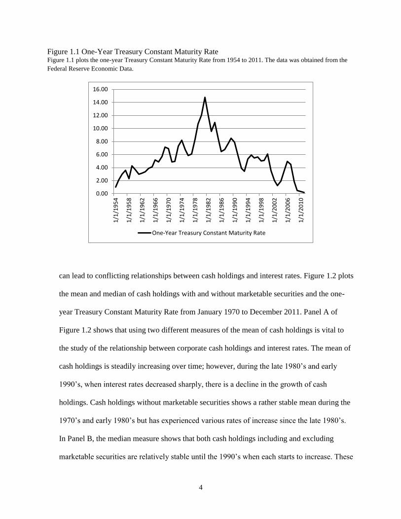
Figure 1.1 plots the one-year Treasury Constant Maturity Rate from January 1954

until December 2011. Beginning in 1954, there is a steady increase in the rate until 1981,

when the rate peaks at 14.78%. The rate then steadily declines to a low of 0.18% in 2011. We

examine how this dramatic swing in the one-year interest rate affected companies’ cash

holdings practices.

While most previous papers have used cash and marketable securities divided by total

assets as the main cash holdings variable, we test both this measure and cash divided by total

assets. The difference between these two variables lies with the marketable securities, which

4

Figure 1.1 One-Year Treasury Constant Maturity Rate Figure 1.1 plots the one-year Treasury Constant Maturity Rate from 1954 to 2011. The data was obtained from the

Federal Reserve Economic Data.

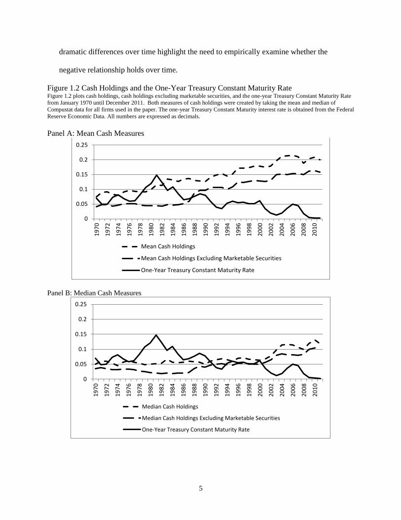
can lead to conflicting relationships between cash holdings and interest rates. Figure 1.2 plots

the mean and median of cash holdings with and without marketable securities and the one-

year Treasury Constant Maturity Rate from January 1970 to December 2011. Panel A of

Figure 1.2 shows that using two different measures of the mean of cash holdings is vital to

the study of the relationship between corporate cash holdings and interest rates. The mean of

cash holdings is steadily increasing over time; however, during the late 1980’s and early

1990’s, when interest rates decreased sharply, there is a decline in the growth of cash

holdings. Cash holdings without marketable securities shows a rather stable mean during the

1970’s and early 1980’s but has experienced various rates of increase since the late 1980’s.

In Panel B, the median measure shows that both cash holdings including and excluding

marketable securities are relatively stable until the 1990’s when each starts to increase. These

0.00

2.00

4.00

6.00

8.00

10.00

12.00

14.00

16.00

1/1

/19

54

1/1

/19

58

1/1

/19

62

1/1

/19

66

1/1

/19

70

1/1

/19

74

1/1

/19

78

1/1

/19

82

1/1

/19

86

1/1

/19

90

1/1

/19

94

1/1

/19

98

1/1

/20

02

1/1

/20

06

1/1

/20

10

One-Year Treasury Constant Maturity Rate

5

dramatic differences over time highlight the need to empirically examine whether the

negative relationship holds over time.

Figure 1.2 Cash Holdings and the One-Year Treasury Constant Maturity Rate Figure 1.2 plots cash holdings, cash holdings excluding marketable securities, and the one-year Treasury Constant Maturity Rate

from January 1970 until December 2011. Both measures of cash holdings were created by taking the mean and median of

Compustat data for all firms used in the paper. The one-year Treasury Constant Maturity interest rate is obtained from the Federal

Reserve Economic Data. All numbers are expressed as decimals.

Panel A: Mean Cash Measures

Panel B: Median Cash Measures

0

0.05

0.1

0.15

0.2

0.25

19

70

19

72

19

74

19

76

19

78

19

80

19

82

19

84

19

86

19

88

19

90

19

92

19

94

19

96

19

98

20

00

20

02

20

04

20

06

20

08

20

10

Mean Cash Holdings

Mean Cash Holdings Excluding Marketable Securities


0

0.05

0.1

0.15

0.2

0.25

19

70

19

72

19

74

19

76

19

78

19

80

19

82

19

84

19

86

19

88

19

90

19

92

19

94

19

96

19

98

20

00

20

02

20

04

20

06

20

08

20

10

Median Cash Holdings

Median Cash Holdings Excluding Marketable Securities


6

The primary contribution of this paper is that it is the first extensive empirical study

of the relationship between interest rates and cash holdings in the United States. While

theoretical relationships were proposed in the 1950’s, they were not examined empirically.

Rather than simply including a measure of interest as a control variable, it is the primary

focus of this paper.

In addition to empirically testing for the relationship between cash holdings and

interest rates, the methodology and data sets are distinguished from recent papers on

corporate cash holdings. The relationship between cash holdings and interest rates is tested

using a random effects threshold model, which distinguishes the relationship over different

ranges of interest rates. Thus, the data are divided into interest rate ranges that are found by

searching for thresholds in the interest rate series. This allows us to see if the negative

relationship holds in the face of the dramatic fluctuation that interest rates experienced during

these times. In addition to testing the relationship for the entire set of observations available

in Compustat, the relationship is tested separately for mature and growth firms. Dividing the

data set in this manner allows us to see if a certain type of firm is driving the results. We also

test alternative explanations for the non-theorized relationship that is found. The relationship

is first tested excluding marketable securities, which is included in most definitions of cash

holdings. These additional tests are based on recent cash holdings papers and are the tax-

based explanation, the cash flow theory, pension fund contributions, zero-leverage firms,

financially constrained and unconstrained firms, firm governance, recessions, and high-tech

firms. None of these relationships fully explain the positive relationship. Finally, in an effort

to find which firms are driving the relationship, quantile regressions are used, which allows

for regressions based on different quantiles of the dependent variable and not the mean as in

7

other models. In doing so, it is found that the positive relationship is driven by firms in the

lower quantiles of cash holdings. Thus, we conclude that the positive relationship that was

found is not driven by any of the above explanations. Instead, it appears that this relationship

is primarily driven by firms with lower cash holdings.

The remainder of the paper is organized as follows: Section 2 discusses the relevant

literature surrounding cash holdings. In Section 3, we put forth the hypotheses and in Section

4 discuss the data. Section 5 presents the model. Section 6 presents the empirical results.

Section 7 examines alternative explanations for the positive relationship discovered between

interest rates and cash holdings. Section 8 presents results based on quantile regressions, and

Section 9 summarizes our findings.

2. Literature Review

The relationship between financial leverage and cash holdings has been well

documented. Prior studies have found that firms decrease their cash holdings as leverage

increases (Opler, et al., 1999; Ozkan and Ozkan, 2004). Guney, et al. (2007) found a non-

linear relationship between cash holdings and leverage and documented a negative

relationship at low levels of financial leverage. However, as leverage increased, the

relationship between cash holdings and leverage became positive which, according to the

authors, was to minimize the risk of financial distress and bankruptcy. Bates, et al. (2009)

documented that net debt experienced a sharp decrease from 1980 until 2006 and was

negative from 2004 until 2006.1 The authors attributed this decrease in debt to an increase in

cash holdings and showed that corporate cash holdings could cover all debt obligations. In

1 Net debt is defined as debt minus cash divided by total assets.

8

addition, they found a decrease in net debt for all size quintiles of companies except the

largest quintile, pointing out that firms in the highest quintile had more leverage in 2006 than

in 1980. Harford, et al. (2013) document a relationship between corporations’ refinancing

risk and cash holdings. More specifically, they found that firms with shorter-maturity debt

hold more cash to compensate for the refinancing risk. This finding explained 28% to 34% of

the increase in corporate cash holdings over the 1980 to 2008 period.

Given the recent attention paid to cash holdings and the extremely low Treasury

security rates, the relationship between interest rates and corporate cash holdings is of

particular interest. However, it has received scant attention in the literature. One of the

earliest papers to examine interest rates and cash is Baumol (1952), who showed that

companies benefit by keeping cash on hand instead of borrowing cash or withdrawing it from

an investment. Tobin (1956) expanded upon Baumol (1952) and showed theoretical evidence

that the demand for cash will depend inversely on the rate of interest. He suggested that

during times of high interest rates, companies will increase holdings of more liquid

investments that earn higher rates and shift into cash only when a transaction must be made.

Meltzer (1963) documented that changes in a firm’s internal rate of return and interest rates

are capable of explaining most of the observed changes in the velocity of business cash

balances. Miller and Orr (1966) suggest that prior models apply reasonably well to

households, but are less than satisfactory when applied to business firms. Their expansion of

Baumol (1952), which allowed for stochastic cash flows leading to stochastic cash balances,

suggested that cash balances fluctuate over time in both directions. However, the model still

finds that cash balances will be a decreasing function of the interest rate. One of the most

widely cited papers on cash holdings, Opler, et al. (1999), used Keynes’s (1936)

9

“transactions-motive” for holding cash. This motive suggests that liquid assets decrease with

interest rates and the slope of the term structure. However, empirical tests did not include

interest rates as an explanatory variable. Ferreira, et al. (2005) looked at business conditions

as a determinant of firms’ cash holdings. They found evidence that cash levels increase

during recessions, especially for financially constrained firms. Using the term spread and the

one-month Treasury bill (T-Bill) rate as two of five proxies for recessions, they documented

that the term spread cannot explain cash holdings but that the one-month T-Bill rate is a

significant determinant of cash holdings.2 Garcia-Teruel and Martinez-Solano (2008)

documented a relationship between interest rates measured as the one-year T-Bill rate, and

cash holdings of small to medium sized firms in Spain from 1996-2001. They found that

when interest rates were at their lowest, cash holdings reached its highest and vice versa. In

the empirical tests, they found a negative relationship between cash holdings and the one-

year T-Bill rate. Bates, et al. (2009) used the three-month T-Bill rate and found a negative

relationship between the log of the cash to total assets ratio and the interest rate. However,

they were unable to verify a statistically significant relationship between their second

measure for cash holdings, cash and marketable securities to total assets, and the T-Bill rate.

Lins, et al. (2010) surveyed Chief Financial Officers (CFOs) in twenty-nine countries to

measure corporate liquidity around the world. The survey questioned CFOs about the

importance they placed on the difference between the interest rate on debt and the interest

rate on cash. Thirty-five percent of responding CFOs rated the difference as highly

important, demonstrating that CFOs take interest rates into account when deciding to hold

cash.

2 Ferreira, et al. (2005) define the term spread as the difference between the long term yield on government bonds

and the one-year T-bill rate.

10

3. Hypotheses

One would expect that based on prior theory corporate cash holdings would have a

negative relationship with interest rates. In other words, as interest rates fall, the opportunity

cost of holding money in investments falls and corporate cash holdings would increase and

vice versa. This leads to our first hypothesis:

Hypothesis 1: The relationship between interest rates and corporate cash holdings should

be negative.

This relationship is examined over the 1970 – 2011 period. However, thresholds are

used to examine smaller intervals of the relationship between interest rates and cash holdings.

As shown in Figure 1.1, during the 1970’s, rates were high and increased over that decade.

This is the only time during the sample where we see a uniform increase in rates. Rates

reached a peak in the early 1980’s but subsequently declined to levels seen during the 1970’s.

In the 1990’s, rates continued to decline, but at a slower pace than was experienced during

the 1980’s. Finally, during the 2000’s and the most recent decade, rates have continued to

decline even further leaving interest rates at the lowest levels experienced over the last forty

years. These dramatic swings in interest rates provide an excellent opportunity to examine

whether the negative relationship exists during each interval.

Hypothesis 1A: The negative relationship should persist in each period.

Finally, the relationship is examined for growth firms and mature firms. Mature and

growth firms are defined based on growth rate of sales where mature (growth) firms are in

the bottom (top) three deciles each year. The data sets are separated because companies in

differing stages might have particular relationships with the differing interest rates. To our

knowledge, the literature has not separated firms in this manner when investigating cash

holdings and interest rates. Growth firms might be more concerned with the interest earned

11

on short term investments and thus it is expected that the relationship between cash holdings

and interest rates for growth firms might not be as large as what would be experienced by

mature firms.

Hypothesis 1B: The negative relationship should be present across both mature and

growth firms, however, mature firms should have a stronger negative relationship.

4. Data

Most variables were obtained from Compustat Annual files unless otherwise noted

and are similar to variables used in Opler, et al. (1999) and previous studies. Financial firms

(SIC 6000-6999) and utilities (SIC 4900-4999) are excluded because cash is held for

business practices and regulatory purposes, respectively. The sample is restricted to firms

headquartered in the United States and firms with complete data for cash and marketable

securities and cash excluding marketable securities. All accounting variables are winsorized

at the lower and upper 1% level.3

The main data set consists of all firms with complete observations in the Compustat

data base from January 1970 until December 2011. The data set contains 183,321 firm-year

observations of more than 15,000 companies. As stated earlier, two additional data sets

consisting of mature and growth firms, respectively, are created. To form these data sets, all

observations in Compustat are sorted into deciles based on the one-year rolling growth rate in

sales.4 The bottom three deciles are defined as mature firms and the top three deciles are

defined as growth firms. The mature firm data set contains 50,542 firm-year observations and

3 In addition, all firms are required to have positive Total Assets and Sales. More than one year of data is required

for all firms after all variables have been calculated. 4 In unreported regressions, growth and mature firms are based on a five-year rolling basis. While, this reduces the

number of observations in each data set to just above 30,000 observations the results remain similar. The main

difference lies within the growth firms, where the middle threshold in the three threshold model is insignificant.

Results are available upon request.

12

covers more than 12,000 firms. The growth firm data set contains 50,523 firm-year

observations and covers more than 14,000 firms. In each data set, firms are allowed to enter

and leave the sample.

The following describes the variables in the data sets:

Cash holdings is defined as cash and marketable securities divided by total assets. It is

used to measure liquidity that a firm has available and will be a positive fractional value.

Cash holdings excluding marketable securities is defined as cash divided by total assets.

Cash is defined by Compustat as “any immediately negotiable medium of exchange or any

instruments normally accepted by banks for deposit and immediate credit to a customer’s

account.”5 Notice that this does leave out marketable securities, which ensures we are

measuring the cash that a firm has and not short term investments. It will be a positive

fractional value.6

Market-to-book ratio is measured as the market value per share to the stated book value

of equity and is used as a measure of growth opportunities that are available to a firm.

Cash flow is earnings after interest, taxes, and dividends, but before depreciation, divided

by total assets. It measures the cash available to the firms after paying normal expenditures

associated with running the firm.

Net working capital is measured as net working capital minus cash and marketable

securities divided by total assets. The standard definition of net working capital does not

subtract cash. However, with cash as the variable of interest, the definition is modified to

5 To be more specific, cash includes a bank or finance company’s receivables, bank drafts, banker’s acceptances,

cash on hand (including foreign currency), certificates of depot included in cash by the company, check (cashier’s or

certified), demand certificates of deposit, demand deposits, letters of credit, and money orders. 6 In unreported regressions, the dependent variable in the baseline regressions are replaced with the log of cash

excluding marketable securities to total assets, the log of cash excluding marketable securities, the log of the ratio of cash holdings excluding marketable securities to one minus the ratio of cash holdings excluding marketable

securities. All results are similar to the results presented here and are available upon request.

13

conform with prior literature. Net working capital is used as a measure for cash substitutes,

as some firms may be able to sell liquid assets instead of using cash holdings.

Capital Expenditure to Assets is capital expenditure divided by total assets and is an

indicator of the expected revenue growth for a firm. Cash holdings and capital expenditure is

expected to have a negative relationship since firms can use cash reserves to fund future

expansion.

Leverage is long term debt plus current debt divided by total assets.7 Leverage measures

the total debt that a company has taken on. This may be an alternative for cash holdings

because some firms may be able to acquire more debt instead of using cash holdings.

Research and development (R&D) to sales is R&D divided by sales. This is also used as

a measure of a firm’s growth opportunities; however, it measures the creative effort that a

firm puts into the growth instead of the market opportunities of growth. If R&D is missing in

Compustat then it is set to zero.

Acquisitions-to-assets are acquisitions divided by total assets. Acquisitions are coded as

zero if Compustat reports a missing value. This measures the growth opportunities that a firm

has experienced through acquiring other companies. Harford (1999) has shown that cash rich

firms make acquisitions and theses are normally value decreasing for the firm.

Dividend Dummy is set equal to one if the company pays a dividend and zero otherwise.

A firm is defined as paying a dividend if a dividend per share is reported in Compustat. Firms

may increase their cash holdings by cutting a dividend that was being paid or by delaying a

dividend payment. No dividend is recorded if Compustat reports the dividend as missing.

Investment Grade Dummy is set equal to one if a company has a bond rating of BBB- and

above, otherwise the dummy equals zero. The bond rating data is obtained from the

7 Current debt is defined in Compustat as long term debt due within one-year and notes payable.

14

Compustat ratings database that contains the Standard & Poor’s (S&P) long term corporate

bond ratings. Bond ratings have been used by previous authors to gauge whether a company

has additional options when accessing funds. An investment grade dummy is included

because a company that has an investment grade may have additional access to bond markets

over non-investment grade companies.8

Size is the natural log of a firm’s total assets in 2005 dollars. The Consumer Price Index

(CPI) is used to account for inflation and is obtained from the Bureau of Labor Statistics.

Large firms have been shown in Opler, et al. (1999) to hold less cash because these firms

have greater access to capital markets.

Cash Flow Riskiness is measured as the standard deviation of industry cash flows

computed by the manner suggested in Opler, et al. (1999).9 It is calculated as the standard

deviation of cash flows for the previous twenty years, if available. We do require that firms

have at least five years of data to calculate cash flow riskiness. Observations are then

averaged across the two-digit SIC code. This measure of industry cash flows is employed

because levels of cash flow can differ greatly across industries.

Interest Rate1, Interest Rate5, and Interest Rate10 are the one-year, five-year, and ten-year

Treasury Constant Maturity Rates, respectively.10

These rates are obtained from the Federal

Reserve Economic Data (FRED).11

Each measures the interest rate that the riskless

government securities are offering. Three different interest rates are included to measure the

short term, intermediate term, and long term relationship with corporate cash holdings. It is

expected that all three interest rates should have a negative relationship with cash holdings.

8 We are aware that bond rating data is comprehensively collected by Compustat starting in 1985. The main results

do not change when this variable is excluded. The results are available upon request. 9 Cash flow used in cash flow riskiness is computed in the manner suggested above by the variable cash flow.

10 The interest rate data in entered into the regressions in decimal format instead of percentage.

11 This was obtained from the website of the Federal Reserve Bank of St. Louis.

15

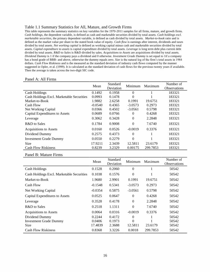
Table 1.1 presents the summary statistics for the variables just described. Panel A

presents the statistics for all firms and Panels B and C are for the mature and growth firms,

respectively. The summary statistics for cash holdings and cash holdings excluding

marketable securities are displayed first in all tables because it is important to note the

difference between the two variables. Cash holdings is larger than cash holdings excluding

marketable securities across all three data sets and both variables ranges from zero to one.12

It was expected that the variables would be different because cash holdings includes short

term investments, which is a significant component of liquid investments for most

companies. It is of interest to note that both the mean of cash holdings and cash holdings

excluding marketable securities are larger for growth firms than mature firms. Further, we

test whether cash holdings and cash holdings excluding marketable securities are

significantly different from one another. In unreported results, cash holdings and cash

holdings excluding marketable securities are statistically different from one another at a 1%

level across all three data sets.

Looking at the other control variables, growth firms have larger net working capital.

In fact, it is positive for growth firms and negative for mature firms suggesting that on

average growth firm’s current assets excluding cash is larger than the current liabilities and

vice versa for mature firms. As expected, growth firms on average have a higher capital

expenditure to assets and acquisitions to assets. Mature firms pay out more dividends and

have investment grade bond rating more often than growth firms. Interestingly, on average

12

It is highly unlikely that a firm would hold all assets as cash. It could be that a mistake was made when collecting

the data. The main results do not change when excluding any observation lying at one. When looking at cash

holdings excluding marketable securities, there are 64 observations that lie at one in the entire data set, 30 in the

mature data set, and 5 in the growth data set.

16

Table 1.1 Summary Statistics for All, Mature, and Growth Firms This table represents the summary statistics on key variables for the 1970-2011 samples for all firms, mature, and growth firms.

Cash holdings, the dependent variable, is defined as cash and marketable securities divided by total assets. Cash holdings excl.

marketable securities, the primary dependent variable, is defined as cash divided by total assets. Market-to-book ratio and is

defined as the market value per share to the stated book value of equity. Cash flow is earnings after interest, dividends and taxes

divided by total assets. Net working capital is defined as working capital minus cash and marketable securities divided by total

assets. Capital expenditure to assets is capital expenditure divided by total assets. Leverage is long term debt plus current debt

divided by total assets. R&D to Sales is R&D divided by sales. Acquisitions to Assets are acquisitions divided by total assets.

Dividend Dummy is 1 if the company pays a dividend and 0 otherwise. Investment Grade Dummy is set equal to 1if a company

has a bond grade of BBB- and above, otherwise the dummy equals zero. Size is the natural log of the firm’s total assets in 1984

dollars. Cash Flow Riskiness and is the measured as the standard deviation of industry cash flows computed by the manner

suggested in Opler, et al. (1999). It is calculated as the standard deviation of cash flows for the previous twenty years if available.

Then the average is taken across the two-digit SIC code.

Panel A: All Firms

Mean Standard

Deviation Minimum Maximum

Number of

Observations

Cash Holdings 0.1492 0.1958 0 1 183321

Cash Holdings Excl. Marketable Securities 0.0993 0.1478 0 1 183321

Market-to-Book 1.9882 2.6258 0.1991 19.6751 183321

Cash Flow -0.0540 0.4365 -3.0573 0.2973 183321

Net Working Capital 0.0366 0.4502 -3.0561 0.5798 183321

Capital Expenditures to Assets 0.0689 0.0766 0 0.4268 183321

Leverage 0.3062 0.3428 0 2.2848 183321

R&D to Sales 0.1784 0.9008 0 7.6740 183321

Acquisitions to Assets 0.0160 0.0526 -0.0019 0.3376 183321

Dividend Dummy 0.2575 0.4373 0 1 183321

Investment Grade Dummy 0.0550 0.2279 0 1 183321

Size 17.9211 2.3439 12.5811 23.6179 183321

Cash Flow Riskiness 0.8239 3.2329 0.00175 299.7853 183321

Panel B: Mature Firms

Mean Standard


Number of

Observations

Cash Holdings 0.1528 0.2060 0 1 50542


Market-to-Book 1.9680 2.9901 0.1991 19.6751 50542

Cash Flow -0.1548 0.5341 -3.0573 0.2973 50542

Net Working Capital -0.0354 0.5875 -3.0561 0.5798 50542


Leverage 0.3528 0.4178 0 2.2848 50542

R&D to Sales 0.2518 1.1311 0 7.6740 50542


Dividend Dummy 0.2244 0.4172 0 1 50542


Size 17.4839 2.3688 12.5811 23.6179 50542


17

Table 1.1 (Continued)

Panel C: Growth Firms

Mean

Standard


Number of

Observations

Cash Holdings 0.1841 0.2193 0 1 50523


Market-to-Book 2.5199 3.0006 0.1991 19.6751 50523

Cash Flow -0.0535 0.4522 -3.0573 0.2973 50523



Leverage 0.2787 0.3238 0 2.2848 50523

R&D to Sales 0.2032 0.8894 0 7.6740 50523


Dividend Dummy 0.1849 0.3882 0 1 50523


Size 17.7074 2.1607 12.5811 23.6179 50523


mature firms have higher R&D to Sales. Growth firms are slightly larger than mature firms.

One might expect mature firms to be larger, however since growth firms are defined using

growth in sales we are capturing some larger firms that are still increasing sales.

Table 1.2 displays some summary statistics on the interest rates and interest rate

thresholds used in the paper. Panel A details statistics for the three interest rates examined in

the paper. While the main focus is placed on the one-year Treasury Constant Maturity Rate,

the relationship between cash holdings and the five and ten-year Treasury Constant Maturity

Rate are also tested.13

The mean of interest rate1 is 5.86% with a large variation in the rate

ranging from 0.1817% to 15.0925%.

13

These results are available upon request.

18

Table 1.2 Threshold and Interest Rate Statistics This table presents summary statistics for the interest rates and thresholds. Interest rate1, interest rate5, and interest rate10 are the

one-year, five-year, and ten-year Treasury Constant Maturity Rate, respectively. All interest rates are reported in decimal terms.

The thresholds were found by minimizing the sum of squared residuals (SSR). The data displayed in Panel C are the distribution

of observations that are in each region for each data set.

Panel A: Statistics on Interest Rates

Mean Standard Deviation Minimum Maximum

Interest Rate1 0.0587 0.0308 0.0018 0.1509

Interest Rate5 0.0663 0.0271 0.0152 0.1454

Interest Rate10 0.0697 0.0248 0.0279 0.1429

Panel B: Threshold Test

Threshold γ1 γ2 γ3 SSR

1 Threshold 0.0587

212.2980

2 Thresholds 0.0348 0.0587

161.81389

3 Thresholds 0.0362 0.0505 0.0788 90.023137

Panel C: Distribution of Observations in Each Region

Threshold Range Entire Mature Growth

1 Threshold Interest Rate1 < γ1 0.5481 0.5601 0.5551

γ1 ≤ Interest Rate1 0.4519 0.4399 0.4449

2 Thresholds Interest Rate1 < γ1 0.1920 0.1991 0.1970

γ1 ≤ Interest Rate1< γ2 0.3561 0.3610 0.3581

γ2 ≤ Interest Rate1 0.4519 0.4399 0.4449

3 Thresholds Interest Rate1 < γ1 0.2308 0.2409 0.2372

γ1 ≤ Interest Rate1 < γ2 0.1249 0.1271 0.1233

γ2 ≤ Interest Rate1 < γ3 0.4163 0.4113 0.4160

γ3 ≤ Interest Rate1 0.2280 0.2207 0.2235

5. Econometric Model

This paper differs from the prior literature and uses a random effects threshold model.

The threshold model allows one to more closely examine the relationship between cash

holdings and interest rates over time. The idea behind using the model is that the relationship

might behave differently when interest rates are within certain thresholds. When simply

19

including the interest rate in the model without thresholds, we do find that there exists a

negative and statistically significant relationship between cash holdings excluding

marketable securities and interest rate1.This is shown in Table 1.3. While the negative

relationship is statistically significant at a 1% level across all the data sets, the economic

significance is small. A one percentage point change in the interest rate represents a decline

in the mean of cash holdings excluding marketable securities of 2.37%. However, Figure 1.2

shows that while there is a general negative relationship between the two variables, this

negative relationship might not hold within different sub-periods. The threshold model

allows us to examine these periods.

The thresholds are based on the level of interest rates. They were found by searching

for the threshold values by minimizing the sum of squared residuals (SSR) from the

regression model that allows for a fixed number of mean-shifts in the level of interest rates.14

Models using one, two, and three thresholds are tested. In each model, the threshold is used

in indicator functions that split the data up into regions. Thus, the one threshold model

divides the sample into two regions, the two threshold model into three regions, and the three

threshold model into four regions. Panel B details the thresholds for the one-year Treasury

Constant Maturity Rate. Each threshold value is identified as γ. γ1 for the one threshold

model is 5.87%. This is close to the mean interest rate of the sample. Panel C displays results

for the percentage of the observations that lie in each indicator function’s region. Looking at

Panel C, roughly 54-56% of all observations in the data sets are below the threshold and the

14

Alternatively, we also used the Bai and Perron (2003) method to detect structural breaks in the data. The Bai and

Perron methodology breaks the data up into time intervals based on structural breaks in the data series. The Bai and

Perron methodology predicts five maximum breaks. The results using four breaks at 1979, 1985, 1991, and 2001

provide similar results to the reported results in that the positive and statistically significant results are found during

the late 1980’s and 1990’s. However, the other time intervals other than the last one from 2001 until 2011 are

insignificant. When using five breaks the relationships are all insignificantly different from zero.

20

remainder are above. γ1 and γ2 for the two threshold model are 3.48% and 5.87%,

respectively. While γ2 is the same threshold value as γ1 in our two threshold model, the

additional threshold breaks up the lower interest rates into two regions. In Panel C, it is

reported that roughly 20% of the observations lie below γ1, 35% of observations are between

γ1 and γ2, and the remaining observations are above γ2. The three thresholds in the final

model are 3.62%, 5.05%, and 7.88%. In Panel C, roughly 25% of observations lie below γ1,

12% are in the range between γ1 and γ2, 40% are between γ2 and γ3, and the remainder are

above γ3.

The interest rate, as well as the interaction between the interest rate and the threshold

dummy, is included in all models. The model is detailed for the two threshold model in

equation 1:

𝑐𝑎𝑠ℎℎ𝑜𝑙𝑑𝑖𝑛𝑔𝑠 𝑒𝑥𝑐𝑙. 𝑚𝑎𝑟𝑘𝑒𝑡𝑎𝑏𝑙𝑒 𝑠𝑒𝑐𝑢𝑟𝑖𝑡𝑖𝑒𝑠𝑖𝑡 = 𝛼0 + 𝛽1𝐼𝑛𝑡𝑒𝑟𝑒𝑠𝑡 𝑅𝑎𝑡𝑒1 𝑡 + 𝛽2 𝐼(𝐼𝑛𝑡𝑒𝑟𝑒𝑠𝑡 𝑅𝑎𝑡𝑒1 𝑡 < γ1)

+ 𝛽3 𝐼( γ1 ≤ 𝐼𝑛𝑡𝑒𝑟𝑒𝑠𝑡 𝑅𝑎𝑡𝑒1 𝑡 < γ2) + 𝛽4(𝐼𝑛𝑡𝑒𝑟𝑒𝑠𝑡 𝑅𝑎𝑡𝑒1 𝑡 ∗ 𝐼(𝐼𝑛𝑡𝑒𝑟𝑒𝑠𝑡 𝑅𝑎𝑡𝑒1 𝑡 < γ1))

+𝛽5(𝐼𝑛𝑡𝑒𝑟𝑒𝑠𝑡 𝑅𝑎𝑡𝑒1 𝑡 ∗ 𝐼( γ1 ≤ 𝐼𝑛𝑡𝑒𝑟𝑒𝑠𝑡 𝑅𝑎𝑡𝑒1 𝑡 < γ2)) + 𝛾𝑋𝑖𝑡 + 𝜀𝑖𝑡 (1)

where 𝑋𝑖𝑡 are the other control variables detailed in the data section. In all models, the

indicator function for the highest interest rate region and the interaction between that region

and the interest rate are omitted from the regression.

When estimating the marginal effect of the interest rate on cash holdings in a

threshold model it is important to not focus solely on the coefficient on the interaction term.

For example, say we want to know the marginal effect of interest rates in the low threshold.

The marginal effect of a change in cash holdings excluding marketable securities by a

change in interest rate1 is given as:

𝜕𝑦

𝜕𝑥= 𝛽1 + 𝛽4 𝐼(𝐼𝑛𝑡𝑒𝑟𝑒𝑠𝑡 𝑅𝑎𝑡𝑒1 𝑡 < γ1) +𝛽5 𝐼( γ1 ≤ 𝐼𝑛𝑡𝑒𝑟𝑒𝑠𝑡 𝑅𝑎𝑡𝑒1 𝑡 < γ2) (2)

21

Table 1.3 Cash Holdings and Interest Rates This table presents the empirical results from the random effects regressions of all firms for 1970-2011. Cash holding excluding

marketable securities is the dependent variable in all regressions. All other variables are defined in Tables 1.1 and 1.2. T-

statistics are in parentheses and significance is denoted by * where the p-value is <.10, ** where the p-value is <.05, and ***

where the p-value is p<.01.

(1) (2) (3)

Entire

Mature

Growth

Market-to-Book 0.00581*** 0.00450*** 0.00695***

(18.15)

(7.54)

(14.85)

Cash Flow 0.0223***

0.00704*

0.0468***

(8.48)

(1.87)

(10.88)

Net Working Capital -0.0272***

-0.0171***

-0.0353***

(-12.68)

(-5.91)

(-8.33)

Capital Expenditures to Assets -0.182***

-0.186***

-0.215***

(-31.59)

(-15.69)

(-23.32)

Leverage -0.0601***

-0.0512***

-0.0641***

(-23.81)

(-12.98)

(-14.75)

R&D to Sales 0.00574***

0.00377**

0.00663***

(4.33)

(2.05)

(3.01)

Acquisitions to Assets -0.184***

-0.187***

-0.212***

(-33.80)

(-10.69)

(-25.79)

Dividend Dummy -0.00104

-0.0000953

-0.000777

(-1.23)

(-0.07)

(-0.46)

Investment Grade Dummy 0.000471

-0.00105

-0.00191

(0.45)

(-0.59)

(-0.74)

Size -0.00265***

-0.00225***

-0.00447***

(-6.18)

(-2.62)

(-6.31)

Cash Flow Riskiness 0.000412***

0.000435*

0.000362*

(4.02)

(1.92)

(1.68)

Lagged Cash Holdings 0.431***

0.562***

0.411***

(77.34)

(60.49)

(56.01)

Lagged Zero Dummy 0.00524*

0.0047

0.00308

(1.88)

(0.90)

(0.57)

Lagged One Dummy -0.151

-0.241

-0.189*

(-1.49)

(-1.59)

(-1.95)

Interest Rate1 -0.235***

-0.240***

-0.275***

(-23.82)

(-13.30)

(-14.38)

Constant 0.0783***

0.0467***

0.0698***

(7.72)

(5.31)

(4.14)

N 161103 48416 46735

Year Dummies No

No

No

Industry Dummies Yes

Yes

Yes

Mundlak-Chamberlain Devices Yes

Yes

Yes

R2 0.529

0.537

0.491

22

where y is cash holdings excluding marketable securities and x is interest rate1. If the

interest rate was below γ1 this would mean the effect was 𝛽1 + 𝛽4. The effect is the linear

combination of the coefficient on interest rate1 and the interaction term. Thus, the marginal

effect when the interest rate is above γ2 is just the coefficient on interest rate1. For brevity, in

all threshold regressions the conditional marginal effects are reported in the table. Interest

rate1 and the interaction of the interest rate and threshold dummy are not reported.

In all models, standard errors are clustered at the firm level. Industry dummies are

included in all models but are not reported.15

Year dummies are tested in the main results, but

are omitted in some models because it was pointed out that including year dummies might

diminish the effect of the across year variations of interest rates. Including year dummies

substantially reduces the variation in the interest rate and thus are excluded in the remaining

analysis.16

One shortcoming of the random effects model is that it assumes that the unobserved

heterogeneity is uncorrelated with the regressors. While this is unlikely, the Mundlak (1978)

and Chamberlain (1980) means relaxes this assumption and allows one to control for the

possible correlations between the unobserved heterogeneity and the regressors. Thus the

Mundlak (1978) and Chamberlain (1980) means are included in the model. The means are

simply the time average of each accounting variable across companies.17

In addition to the variables described in Section 4, several other control variables are

included in the model. Lagged cash holdings is included in the model and is defined as cash

15

Industry dummies are based on two-digit SIC code. 16 These results are available upon request. 17

The time means for the Mundlak (1978) and Chamberlain (1980) devices are included in all models but their

coefficients are not reported.

23

holdings from the previous year.18

This is included for both measures of cash holdings due to

the highly stable nature of cash holdings within firms. While the models support values at

zero and one, additional variables to control for values at these corners are included. Lag zero

dummy is set equal to one if the lagged cash holdings variable is zero and is set equal to zero

otherwise. Lag one dummy is set equal to one if the lagged cash holdings variable is one and

is set equal to zero otherwise.

6. Estimation Results and Interpretations

In preliminary regressions, numerous positive relationships were found between cash

holdings and interest rate1 when using the threshold model.19

The majority of the

relationships were statistically significant at conventional levels. One possible explanation is

that because cash holdings contain cash and marketable securities, it could be picking up on

the relationship between the short term investments and the interest rates. Thus, as the

interest rates decline, companies might move money from investments to cash due to the

lower opportunity cost and lower returns. This positive relationship between the short term

investments and interest rates might be overpowering the relationship between the levels of

cash and interest rates. It is expected that a negative relationship between cash holdings

excluding marketable securities and interest rates exists. Thus, the results using the

dependent variable cash holdings excluding marketable securities are reported. The results

18

In unreported results, all baseline regressions are run excluding the lagged dependent variable. Results are similar

among the three threshold model however, some results do lose significance. These results are available upon

request. 19


24

using the two and three threshold models are shown in Tables 1.4 and 1.5 and are discussed

below.20

6.1 Two Threshold Model

The results testing for the relationship between cash holdings and interest rates using

the two threshold model are presented in Table 1.4. Column 1 report the results for the entire

data set, while Column 2 report the results for the mature firm data set and Column 3 reports

the results for the growth firm data set.

First, we want to direct your attention to the marginal effect for the relationship

between interest rate1 and cash holdings excluding marketable securities located at the

bottom of the table. As expected, the relationship between cash holdings excluding

marketable securities and interest rates in low region is negative and statistically significant

at a 1% level across all three data sets. The interesting results arise when looking at the

relationship between interest rates in middle region and cash holdings excluding marketable

securities. The relationship is not statistically different from zero in the entire and mature

data set and is positive and statistically significant at a 1% level in the growth data set. This

is not as hypothesized. The relationship between cash holdings excluding marketable

securities and interest rates in high region is negative and statistically significant at a 1%

level across all three data sets.

Not only is the relationship between the cash holdings of growth firms and interest

rate1 in the middle region statistically significant but it is also economically significant. A

one percentage point change in interest rate1 increases cash holdings excluding marketable

20

Results based on the one threshold are reported in Appendix Table A.1.1. Because the groups are larger in the one

threshold model, negative and statistically significant relationships were found across both groups. This is not

unexpected.

25

Table 1.4 Cash Holdings and Interest Rates with Two Thresholds This table presents the empirical results from the random effects threshold regressions of all firms for 1970-2011. Cash holding

excluding marketable securities is the dependent variable in all regressions. All other variables are defined in Tables 1.1 and 1.2.

T-statistics are in parentheses and significance is denoted by * where the p-value is <.10, ** where the p-value is <.05, and ***


(1) (2) (3)

Entire

Mature

Growth

Market-to-Book 0.00575*** 0.00443*** 0.00685***

(17.91)

(7.40)

(14.59)

Cash Flow 0.0224***

0.00714*

0.0465***

(8.51)

(1.89)

(10.84)


-0.0169***

-0.0359***

(-12.57)

(-5.84)

(-8.46)


-0.186***

-0.217***

(-31.45)

(-15.62)

(-23.49)

Leverage -0.0600***

-0.0510***

-0.0643***

(-23.76)

(-12.94)

(-14.76)

R&D to Sales 0.00584***

0.00390**

0.00664***

(4.40)

(2.12)

(3.03)


-0.186***

-0.214***

(-33.49)

(-10.59)

(-25.99)


-0.000187

-0.000131

(-1.29)

(-0.14)

(-0.08)


-0.000504

-0.00263

(0.58)

(-0.28)

(-1.02)

Size -0.00301***

-0.00263***

-0.00448***

(-6.77)

(-2.98)

(-6.07)


0.000443*

0.000460**

(4.13)

(1.94)

(2.34)


0.561***

0.410***

(77.24)

(60.25)

(55.88)


0.00474

0.0026

(1.85)

(0.91)

(0.48)


-0.239

-0.185*

(-1.47)

(-1.58)

(-1.92)

I(Interest Rate1 < γ1) 0.0105***

0.0142***

0.000968

(5.74)

(4.15)

(0.25)

I(γ1 ≤ Interest Rate1 < γ2) -0.00789**

-0.00272

-0.0395***

(-2.35)

(-0.41)

(-5.17)

Interest Rates in Low Region -0.4714***

-0.5573***

-0.4499***

(-7.69)

(-4.82)

(-3.45)

Interest Rates in Middle Region 0.0620

-0.0061

0.6120***

(0.99)

(-0.05)

(4.27)

26


Interest Rates in High Region -0.1798***

-0.1597***

-0.2904***

(-15.27)

(-7.08)

(-11.25)

Constant 0.0750***

0.0418***

0.0717***

(7.45) (4.78) (4.29)

N 161103

48416

46735

Year Dummies No

No

No


Yes

Yes


Yes

Yes

R2 0.529 0.538

0.492

securities by 0.00612. While this does not seem like a large amount it represents a 5%

increase in the mean values of cash holdings (0.1204). Going from the lowest end of the

threshold to the highest end of the threshold is an increase in 2.39%. This increases cash

holdings excluding marketable securities by 0.0146 or a 12% increase in the mean value.

A quick look at the control variables shows results similar to prior papers in cash

holdings. Market-to-book is positively and significantly related to cash holdings excluding

marketable securities implying that firms with more growth opportunities hold more cash.

Cash flow is also positively related to cash holdings excluding marketable securities

suggesting that firms with more cash flow hold more cash in general. Capital expenditures to

assets and acquisitions to assets are both negatively related to cash holdings excluding

marketable securities at a 1% level implying that firms with these expenditures hold less

cash. Firms that have an investment grade bond rating (investment grade dummy) and are

larger (size) hold less cash, a finding that is significant at a 1% level. Leverage is

significantly negatively related to cash holdings suggesting that firms with larger amounts of

debt hold less cash. Prior literature had suggested that the relationship could be positive or

negative, but we find that the larger interest payments associated with larger amounts of debt

27

lead firms to hold less cash. The main difference in our results among control variables is

that no relationship is found between firms that pay dividends (dividend dummy) and cash

holdings excluding marketable securities. Prior papers have found that firms that paid more

in dividends held less cash. Finally, lagged cash holdings has a positive relationship that is

significant at a 1% level with cash holdings. The lagged zero dummy and lagged one dummy

are primarily insignificant across all data sets.

In summary, when testing for the relationship between corporate cash holdings and

interest rates a negative relationship is expected. While the negative relationship is found

when examining the entire time period from 1970-2011, when testing a threshold model

either a positive or insignificant relationship is found. The relationship is found among

interest rates in middle region, which covers rates from 3.48% to 5.87%. These rates

occurred primarily during the late 1990’s when interest rates were declining from the peak

experienced during the 1980’s. This has not been documented in the literature. In an attempt

to explain why this relationship exists, additional controls are included in Section 7.

6.2 Three Threshold Model

The results testing for the relationship between cash holdings and interest rates using

a three threshold model are presented in Table 1.5. As in Table 1.3, Column 1 reports the

results for the entire data set, while Column 2 reports the results for the mature firm data set,

and Column 3 reports the results for the growth firm data set.

The marginal effect between interest rates in the different regions and cash holdings

are presented at the bottom of the table. Again, the relationship between cash holdings

excluding marketable securities and interest rates in low region is negative and statistically

28

Table 1.5 Cash Holdings and Interest Rates with Three Thresholds This table presents the empirical results from the random effects threshold regressions of all firms for 1970-2011. Cash holding

excluding marketable securities is the dependent variable in all regressions. All other variables are defined in Tables 1.1 and 1.2.

T-statistics are in parentheses and significance is denoted by * where the p-value is <.10, ** where the p-value is <.05, and ***


(1) (2) (3)

Entire

Mature

Growth

Market-to-Book 0.00580*** 0.00445*** 0.00684***

(18.03)

(7.44)

(14.55)

Cash Flow 0.0224***

0.00722*

0.0467***

(8.53)

(1.92)

(10.88)


-0.0169***

-0.0360***

(-12.59)

(-5.85)

(-8.46)


-0.186***

-0.216***

(-31.45)

(-15.64)

(-23.45)

Leverage -0.0601***

-0.0511***

-0.0644***

(-23.78)

(-12.96)

(-14.78)

R&D to Sales 0.00583***

0.00390**

0.00668***

(4.39)

(2.12)

(3.04)


-0.186***

-0.214***

(-33.41)

(-10.57)

(-25.91)


-0.000207

-0.000114

(-1.42)

(-0.15)

(-0.07)


-0.000282

-0.00238

(0.88)

(-0.16)

(-0.92)

Size -0.00287***

-0.00254***

-0.00459***

(-6.44)

(-2.88)

(-6.24)


0.000451**

0.000469**

(4.08)

(1.97)

(2.41)


0.562***

0.410***

(77.31)

(60.34)

(55.90)


0.00464

0.00263

(1.90)

(0.89)

(0.49)


-0.24

-0.186*

(-1.48)

(-1.59)

(-1.92)

I(Interest Rate1 < γ1) 0.00715***

0.0130***

0.00461

(3.13)

(2.84)

(0.97)

I(γ1 ≤ Interest Rate1 < γ2) -0.0252***

-0.0491***

-0.0392**

(-3.34)

(-3.20)

(-2.15)

I(γ2 ≤ Interest Rate1 < γ3) 0.00562

0.0148**

0.0341***

(1.49)

(1.98)

(3.94)


-0.3948***

-0.5026***

(-8.31)

(-4.07)

(-4.85)

29


Interest Rates in Lower Middle Region 0.3768**

0.9800***

0.6697*

(2.33)

(3.02)

(1.72)

Interest Rates in Upper Middle Region -0.2767***

-0.3472***

-0.7293***

(-5.32)

(-3.42)

(-6.09)


-0.1543***

-0.2647***

(-11.84)

(-4.39)

(-7.22)

Constant 0.0764***

0.0406***

0.0696***

(7.51) (4.36)

(4.08)

N 161103

48416

46735

Year Dummies No

No

No


Yes

Yes


Yes

Yes

R2 0.529 0.538

0.492

significant at a 1% level across all three data sets. The interesting results arise when looking

at the relationship between interest rates in lower middle region and cash holdings excluding

marketable securities. The relationship is positive and statistically significant across all three

data sets. This is not as hypothesized. The significance does vary from a 5% level in the

entire data set, a 1% level in the mature data set, and a 10% level in the growth data set.

Interest rates in upper middle region are negatively and statistically related to cash holding

excluding marketable securities at a 1% level in all three data sets. A negative and significant

relationship at a 1% level between interest rates in high region and cash holdings excluding

marketable securities is found.

In the lower middle region, the relationship between cash holdings excluding

marketable securities and interest rates has economic as well as statistical significance. When

looking at the entire data set, a one percentage point change in interest rate1 increases cash

holdings excluding marketable securities by 0.0038. This represents a 3.8% increase in the

mean value of cash holdings excluding marketable securities (0.0993). In the mature data

set, an increase in interest rate1 of one percentage point increases cash holdings excluding

30

marketable securities by 0.0098. This represents an increase of 9.4% of the mean value of

cash holdings excluding marketable securities (0.1038). Among growth firms, an increase in

interest rate1 increases cash holdings excluding marketable securities by 0.0067. This

represents an increase of 5.6% of the mean value of cash holdings excluding marketable

securities. This result is greatly enhanced when looking at a change in the entire range of

interest rates in the region.

In review, the relationship between cash holdings and interest rates in the range of

3.62% and 5.05% is found to be positive. The results are tested using the three threshold

model to narrow down the range of rates in which the relationship is positive. The results

show that the relationship between cash holdings excluding marketable securities and

interests rates during this range, which is primarily found during the 1990’s, is not as

hypothesized by prior literature. Again, in an attempt to explain why this relationship exists,

additional controls are included in Section 7.

7. Tests for the Non-Negative Relationship

Given that it has been determined that the positive relationship was not driven

completely by the marketable securities included in cash holdings, we attempt to explain why

the relationship exists. Recall that the positive and significant relationships and insignificant

relationships exist primarily in the middle region (0.0348 ≤ Interest Rate1 < 0.0587) of the

two threshold model and the lower middle region (0.0362 ≤ Interest Rate1 < 0.0505) of the

three threshold model. Thus, we control for other factors that might be driving the positive

relationship during this time. Several additional explanations for the positive relationship are

tested and discussed below. These explanations are the tax-based explanation, cash flow

31

theory, pension fund contributions, zero-leverage firms, financially constrained and

unconstrained firms, firm governance, recessions, and high-tech firms.

7.1 Tax-Based Explanation

Originally introduced by Foley, et al. (2007), the tax-based explanation suggests that

firms facing higher repatriation taxes hold larger levels of cash, hold the cash abroad, and

hold the cash in places that trigger high tax costs when repatriating earnings. The Association

for Financial Professionals reports that due to high tax rates, United States multinational

corporations have $1 trillion in cash and cash equivalent investments outside of the United

States.21,22

In 2004, Congress enacted the Homeland Investment Act (HIA) which temporary

reduced the tax to 5.25% and repatriation surged. Pinkowitz, et al. (2012) find that the HIA

did not reduce cash holdings of multinational firms and put forth two possible explanations:

either the incentives in the HIA were insufficient to affect corporate cash holdings or the HIA

changed where firms store there cash and not the amount held. It is possible that companies

holding cash abroad are forgoing the interest that could be earned in the Treasury market.

Thus, we may be picking up on the relationship between the foreign cash holdings and the

interest rate, which would be a spurious relationship.

A multinational firm is defined as a firm that reports pretax foreign income in

Compustat.23

The data sets are divided into domestic and multinational companies based on

this criterion. For the tax-based explanation to be valid, it is expected that when dividing the

21

Available at http://www.afponline.org/search.aspx?searchtext=repatriation in the “AFP Policy Position on

Repatriation.” 22

A multinational firm is a firm that reports operations in a foreign country but is incorporated in the United States. 23

If Compustat reports that pretax foreign income is missing the value is coded as zero. Similar results are obtained

if the Compustat variable IDBFLAG (international, domestic, and both indicator) is used. However, using this

variable reduced the sample of multinational companies. Thus, results are presented using pre-tax foreign income in

the paper and the results using IDBFLAG are available upon request.

32

data sets into domestic and multinational firms, the positive relationship should exist only in

the multinational sample. Over this time, the relationship between cash holdings excluding

marketable securities and the interest rates should be negative for the domestic firms.

Results can be found using the two threshold model in Table 1.6.24

For brevity, only

the coefficients for the marginal effects of the interest rates are reported. Columns 1 and 2

present results for the entire sample when divided into domestic and multinational firms,

respectively. Columns 3 and 4 are for the mature domestic and multinational firms and

Columns 5 and 6 present results for the growth domestic and multinational firms. It is seen

that the positive relationship is still prevalent amongst the domestic firms primarily in the

interest rates in middle region (γ1 ≤ Interest Rate1 < γ2). The relationship is significant at a

1% level in the entire and growth data sets and positive but not statistically different from

zero in the mature data set. An interesting result is found when looking at the multinational

companies; the relationship between cash holdings excluding marketable securities and

interest rates in middle region is negative and statistically significant for the entire sample

and mature sample and positive but not statistically different from zero amongst the growth

firms. Thus, it seems that the reason for the positive relationship cannot be explained by

firms holding cash overseas.

7.2 Sources of Cash Flow

In addition to the tax-based explanation, operating and investing cash flow are

examined. It has been shown that cash savings from operating cash flow has decreased in the

past 20 years (McLean, 2011). However, if a company issues bonds, then an overall positive

24

Results for the three threshold model can be found in Appendix Table A.1.2. The results are similar to those

discussed here.

33

Table 1.6 Tax-Based Explanation This table presents the empirical results for all, mature, and growth firms when controlling for the tax based explanation. Multinational firms are defined as firms that report pretax

foreign income in Compustat. Cash Holdings excluding marketable securities is the dependent variable in all regressions. This table presents only the interest rate variables. All

other variables are defined in Tables 1.1 and 1.2. T-statistics are in parentheses and significance is denoted by * where the p-value is <.10, ** where the p-value is <.05, and ***


(1) (2)

(3) (4)

(5) (6)

Entire

Mature

Growth

Domestic Multinational Domestic Multinational Domestic Multinational

I(Interest Rate1 < γ1) 0.00942*** 0.0221***

0.0140*** 0.00211

0.00141 -0.0246**

(3.90) (3.64)

(3.30) (0.25)

(0.30) (-2.03)

I(γ1 ≤ Interest Rate1 < γ2) -0.0133*** 0.0199***

-0.00982 0.00728

-0.0422*** -0.0395**

(-3.20) (2.75)

(-1.21) (0.60)

(-4.84) (-2.37)

Interest Rates in Low Region -0.4242*** -0.4346***

-0.5116*** -0.5509***

-0.4258*** -0.4001**

(-4.91) (-5.93)

(-3.27) (-4.03)

(-2.57) (-2.05)

Interest Rates in Middle Region 0.1894** -0.2485***

0.1519 -0.3936**

0.6959*** 0.1060

(2.41) (-2.75)

(0.99) (-2.19)

(4.23) (0.40)

Interest Rates in High Region -0.1691*** 0.0670

-0.1507*** -0.2340**

-0.2787*** -0.5220***

(-13.59) (0.82)

(-6.46) (-2.23)

(-10.44) (-3.64)

N 129523 28020 39961 8455 40109 6626

Year Dummies No No

No No

No No

Industry Dummies Yes Yes

Yes Yes

Yes Yes

Mundlak-Chamberlain Devices Yes Yes

Yes Yes

Yes Yes

R2 0.514 0.635

0.524 0.643

0.484 0.561

34

inflow of cash might exist. The inflow of investing cash would increase cash holdings, and at

the same time, the issuance of the bonds would occur at low interest rate periods, which

might contribute to the positive relationship. The rates during the middle region align with

interest rates during the 1990’s. Although the rates during the 1990’s were not as low as they

are currently, they were very low relative to the interest rates in the late 1970’s and 1980’s.

This could contribute to the reason why a positive relationship was seen in the middle region.

Almeida, et al. (2004) found that financially constrained firms’ cash holdings should increase

when cash flows are higher; they call this the “cash flow sensitivity of cash.” They find that

unconstrained firms should display no pattern.

The operating cash flow and investing cash flow information was obtained from

Compustat annual files.25

The results can be found in Table 1.7. The coefficients from both

cash flow variables are reported as well as the marginal effect for the interest rate regions.

The results from the entire data set are displayed in Columns 1 and 2, the results from the

mature data set are displayed in Columns 3 and 4, and the results from the growth data set are

displayed in Columns 5 and 6. The odd columns display the results from the two threshold

model and the even columns display the results for the three threshold model.

In all regressions, both operating cash flow and investing cash flow are positive and

statistically significant at a 1% level. Overall, the relationships between the interest rate

regions and cash holdings excluding marketable securities remain unchanged. When looking

at the entire data set, the relationship between cash holdings excluding marketable securities

and interest rates in middle region in the two threshold model goes from being insignificant

to positive and significant at a 1% level. In the three threshold model, the relationship in the

25

The operating and investing cash flow were both added after removing the cash flow variable described in Section

4.

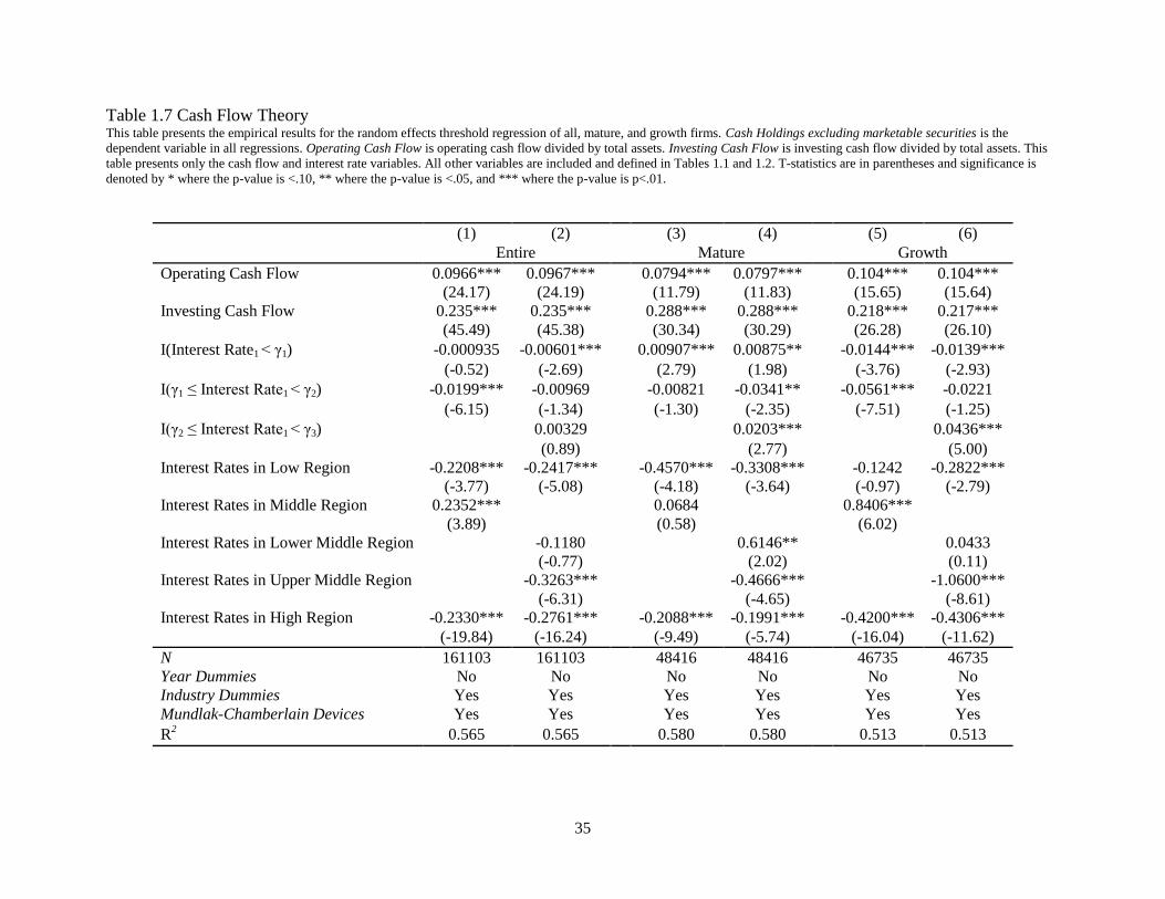
35

Table 1.7 Cash Flow Theory This table presents the empirical results for the random effects threshold regression of all, mature, and growth firms. Cash Holdings excluding marketable securities is the

dependent variable in all regressions. Operating Cash Flow is operating cash flow divided by total assets. Investing Cash Flow is investing cash flow divided by total assets. This

table presents only the cash flow and interest rate variables. All other variables are included and defined in Tables 1.1 and 1.2. T-statistics are in parentheses and significance is

denoted by * where the p-value is <.10, ** where the p-value is <.05, and *** where the p-value is p<.01.

(1) (2) (3) (4) (5) (6)

Entire

Mature

Growth

Operating Cash Flow 0.0966*** 0.0967***

0.0794*** 0.0797***

0.104*** 0.104***

(24.17) (24.19)

(11.79) (11.83)

(15.65) (15.64)

Investing Cash Flow 0.235*** 0.235***

0.288*** 0.288***

0.218*** 0.217***

(45.49) (45.38)

(30.34) (30.29)

(26.28) (26.10)

I(Interest Rate1 < γ1) -0.000935 -0.00601***

0.00907*** 0.00875**

-0.0144*** -0.0139***

(-0.52) (-2.69)

(2.79) (1.98)

(-3.76) (-2.93)

I(γ1 ≤ Interest Rate1 < γ2) -0.0199*** -0.00969

-0.00821 -0.0341**

-0.0561*** -0.0221

(-6.15) (-1.34)

(-1.30) (-2.35)

(-7.51) (-1.25)

I(γ2 ≤ Interest Rate1 < γ3)

0.00329

0.0203***

0.0436***

(0.89)

(2.77)

(5.00)


-0.4570*** -0.3308***

-0.1242 -0.2822***

(-3.77) (-5.08)

(-4.18) (-3.64)

(-0.97) (-2.79)

Interest Rates in Middle Region 0.2352***

0.0684

0.8406***

(3.89)

(0.58)

(6.02)

Interest Rates in Lower Middle Region

-0.1180

0.6146**

0.0433

(-0.77)

(2.02)

(0.11)

Interest Rates in Upper Middle Region

-0.3263***

-0.4666***

-1.0600***

(-6.31)

(-4.65)

(-8.61)

Interest Rates in High Region -0.2330*** -0.2761***

-0.2088*** -0.1991***

-0.4200*** -0.4306***

(-19.84) (-16.24)

(-9.49) (-5.74)

(-16.04) (-11.62)

N 161103 161103 48416 48416 46735 46735

Year Dummies No No

No No

No No


Yes Yes

Yes Yes


Yes Yes

Yes Yes

R2 0.565 0.565 0.580 0.580 0.513 0.513

36

lower middle region falls in significance from a 5% level to being insignificantly different

from zero. Similar results are observed for mature firms as results reported earlier. Looking

at the growth firms, similar results are seen as with the entire firms with the relationships

during the three threshold model going from statistically significant to insignificantly

different from zero.

Therefore, while it can be seen that controlling for investing and operating cash flow

removes some of the positive and statistically significant relationships in the lower middle

region, a negative relationship still is not found. Thus, other explanations are tested to see if

they result in the expected negative relationship.

7.3 Pension Fund Contributions

An additional test for an explanation for the positive relationship is that cash

contributions made to pension funds during the 1980’s and the 1990’s were greater and thus

larger amounts of cash were held to meet these obligations. According to the Employee

Retirement Income Security Act of 1974, the contributions made to defined benefit (DB)

pension funds are annually reviewed to ensure that the plans are funded accordingly. DB

plans were the most popular form of pension plan in the 1980’s and the 1990’s. During times

of economic turmoil, there is a chance that investments might fall below the well-funded

level. In these cases, a company will have to make larger contributions and these

contributions are often made with liquid corporate assets (Rauh, 2009). Rauh (2006) showed

that cash for required contributions leads to lower capital investment. Thus, the companies in

the 1980’s and the 1990’s might have been holding more cash due to the larger cash

contributions that were required. During this time, the economy did experience three

37

recessions so the poor market performance that has not been accounted for could be a

contributing factor.26

The pension fund contribution hypothesis is tested using two different

variables. The first variable is pension expense to total assets. The second variable is the

mandatory pension variable used in Campbell, et al. (2012). It measures the mandatory

pension expense required to maintain well-funded status. It is calculated by the service costs

plus the accumulated benefit obligation minus the fair value of pension plan assets divided by

30. This is all divided by total firm assets as of the previous year. This is calculated if the

pension benefit obligation is greater than the fair value of pension plan assets. Both measures

are obtained from data found in Compustat Annual Pension database and Compustat Annual

Files. If a variable is missing then it is recorded as zero. Due to the similarity between the

results, we report the results using pension expense and include the results using mandatory

pension expense in appendix Table A.1.3.27

The predicted relationship between cash holdings excluding marketable securities

and the pension expense variables is negative. Thus, as pension expense increases, the cash

holdings of the firm will decrease and vice versa. This is done to account for the excess cash

contributions that a company may have to make to ensure the plans are funded accordingly.

The results can be found in Table 1.8. For brevity, only the pension expense variable

and interest rate regions are reported. Again the table is laid out in a similar fashion as

previous tables with the results from the entire data set are displayed in Columns 1 and 2, the

results from the mature data set are displayed in Columns 3 and 4, and the results from the

26

The list of recessions is obtained from the NBER and the recessions are over January 1980 to July 1980, July

1981 to November 1982, and July 1990 to March 1991. 27

As seen in the appendix, mandatory pension expense is not statistically significant in any of the regressions and

the results remain unchanged from results previously reported.

38

Table 1.8 Pension Fund Contributions This table presents the empirical results for the random effects threshold regressions of all, mature, and growth firms. Cash Holdings excluding marketable securities is the

dependent variable in all regressions. Pension Expense is defined as the reported pension expense in Compustat divided by total assets. If pension expense is missing then it is set

to zero. This table presents only the results for the pension expense variable and interest rates. All other variables are included and defined in Tables 1.1 and 1.2. T-statistics are in

parentheses and significance is denoted by * where the p-value is <.10, ** where the p-value is <.05, and *** where the p-value is p<.01.

(1) (2) (3) (4) (5) (6)

Entire Mature Growth

Pension Expense -0.191*** -0.193***

-0.0622 -0.0648

-0.640*** -0.644***

(-3.46) (-3.47)

(-0.63) (-0.66)

(-5.10) (-5.13)

I(Interest Rate1 < γ1) 0.0109*** 0.00772***

0.0144*** 0.0133***

0.00151 0.00541

(5.90) (3.36)

(4.16) (2.88)

(0.39) (1.13)

I(γ1 ≤ Interest Rate1 < γ2) -0.00759** -0.0253***

-0.00258 -0.0491***

-0.0392*** -0.0393**

(-2.26) (-3.35)

(-0.38) (-3.20)

(-5.13) (-2.16)


0.00581

0.0148**

0.0344***

(1.54)

(1.98)

(3.98)


-0.5583*** -0.3957***

-0.4565*** -0.5078***

(-7.74) (-8.37)

(-4.83) (-4.08)

(-3.50) (-4.89)


-0.0074

0.6110***

(0.96)

(-0.06)

(4.27)


0.3899**

0.9855***

0.6857*

(2.41)

(3.04)

(1.77)


-0.2724***

-0.3434***

-0.7245***

(-5.23)

(-3.38)

(-6.04)


-0.157*** -0.151***

-0.283*** -0.255***

(-14.78) (-11.39)

(-6.96) (-4.29)

(-10.96) (-6.96)

N 161103 161103 48416 48416 46735 46735

Year Dummies No No

No No

No No


Yes Yes

Yes Yes


Yes Yes

Yes Yes

R2 0.529 0.529

0.538 0.538 0.492 0.492

39

growth data set are displayed in Columns 5 and 6. The odd columns display the results from

the two threshold model and the even columns display the results for the three threshold

model.

Pension expense is negative and significantly related to cash holding excluding

marketable securities at a 1% level in the entire data set and the growth data set. The

relationship is insignificant for mature firms. When looking at the marginal effect, little to

no change in the relationships between the interest rate regions and cash holdings excluding

marketable securities are seen across all three models. In conclusion, while pension expense

is of the predicted sign and is statistically significant in the regressions it does not explain the

positive relationship between cash holdings excluding marketable securities and interest

rates.

7.4 Zero-Leverage Firms

The mystery of why firms choose not to hold any debt has led researchers to look into

the characteristics of these companies. As reported in Strebulaev and Yang (2013), 14% of

large public non-financial US firms had zero outstanding debt in 2000. In addition, they find

that zero-leverage firms and particularly dividend-paying, zero-leverage firms have higher

cash balances than matched firms. In fact, they find that 75% of the time zero-leverage firms

hold higher levels of cash than the matched firms. It could be the case that the results are

being driven by the zero-leverage firms.

In the entire data set, zero-leverage firms are holdings substantial amounts of cash

holdings and cash holdings excluding marketable securities. The mean of cash holdings and

cash holdings excluding marketable securities for zero-leverage firms and firms with

leverage is presented in appendix Table A.1.4. The mean measure of cash holdings for zero-

40

Table 1.9 Excluding Zero-Leverage Firms This table presents the empirical results for the random effects threshold regressions of all, mature, and growth firms. Cash Holdings excluding marketable securities is the

dependent variable in all regressions. Firms with zero-leverage are deleted from the sample. All other variables are included and defined in Tables 1.1 and 1.2. T-statistics are in


(1) (2) (3) (4) (5) (6)


I(Interest Rate1 < γ1) 0.00940*** 0.00434**

0.0128*** 0.00834*

-0.00165 -0.000973

(5.38) (2.00)

(4.00) (1.93)

(-0.42) (-0.21)


0.000833 -0.0302**

-0.0387*** -0.0489***

(-2.13) (-3.18)

(0.13) (-2.08)

(-5.13) (-2.81)

I(γ2 ≤ Interest Rate1 < γ3) -0.00412

0.00909

0.0199**

(-1.17)

(1.33)

(2.45)


-0.4854*** -0.3081***

-0.3458*** -0.3900***

(-7.36) (-7.84)

(-4.41) (-3.31)

(-2.56) (-3.68)


-0.0510

0.5704***

(0.58)

(-0.43)

(4.04)


0.2749*

0.5250*

0.7698**

(1.85)

(1.73)

(2.08)


-0.1347***

-0.2740***

-0.5369***

(-2.80)

(-3.00)

(-4.70)


-0.1214*** -0.1431***

-0.2602*** -0.2606***

(-14.72) (-12.45)

(-6.05) (-4.50)

(-10.57) (-7.50)

N 144048 144048 42898 42898 40908 40908

Year Dummies No No

No No

No No


Yes Yes

Yes Yes


Yes Yes

Yes Yes

R2 0.474 0.473

0.482 0.482

0.448 0.448

41

leverage firms ranges from 0.23122 in 1970 to 0.40551 in 2011. The variation in cash

holdings excluding marketable securities is just as drastic ranging from 0.04871 in 1970 to

0.29885 in 2011. This mean is substantially above the mean of cash holdings and cash

holdings excluding marketable securities for firms with leverage. It is also of interest to test

the relationship excluding the zero-leverage firms because a substantial increase in the mean

of cash holdings excluding marketable securities for zero-leverage firms takes place in 1988,

which is when the large increase shown in Panel A of Figure 1.2 takes place. Thus, the

baseline regressions are repeated excluding zero-leverage firms (17,055 firm-year

observations).

The results are presented in Table 1.9.28

Again focusing on the marginal results for

the interest rate thresholds, the results remain very similar to those seen in Tables 1.4 and 1.5.

Particularly when looking at the two threshold model, the relationship between cash holdings

excluding marketable securities and interest rate1 when the interest rate falls within the

middle region is not statistically different from zero in the entire and mature data sets and is

positive and statistically significant at a 1% level for mature firms. The main change in the

results takes place in the three threshold model. The relationship between cash holdings

excluding marketable securities and the interest rates in lower middle region remains

positive and statistically significant among all data sets however, it does lose significance in

the entire and mature firm data sets when testing three thresholds. Thus, zero-leverage firms

are not driving the results.

28

In unreported results, almost zero-leverage firms are also excluded. Strebulaev and Yang (2013) classify almost

zero-leverage firms as firms whose leverage ratio is less than 5% (an additional 16,969 firm-year observations).

Similar results are found as when excluding zero-leverage firms and the baseline regression. These results are

available upon request.

42

7.5 Constrained and Unconstrained Firms

In an additional test, the relationship is examined across financially constrained and

unconstrained firms. Almeida, et al. (2004) show that constrained manufacturing firms, when

measured by firm size, bond rating, and commercial paper, hold more cash than

unconstrained manufacturing firms. Thus, it could be that the constrained firms are holdings

more cash for financial reasons and are not taking into account interest rates when holdings

cash.

We follow Almeida, et al. (2004) and define financially constrained firms three

different ways.29

The first is based on firm size. Firms are sorted into deciles each year based

on total assets and the top (bottom) three deciles are defined as unconstrained (constrained)

firms. The argument is that smaller firms are typically younger and less well known. The

second and third measures are bond and commercial paper ratings. These are measured

similarly, with the exception that the bond rating data is the S&P long-term rating and the

commercial rating data is the S&P short-term rating. If a firm has never had a rating and

holds a positive value for debt then the firm is classified as constrained. Unconstrained firms

are classified as firms that have been rated during the sample.30

The argument here is that

firms without ratings do not have the ease of access to external financing.

Table 1.10 displays the mean of cash holdings and cash holdings excluding

marketable securities for constrained and unconstrained firms. All three measures of

financial constraint provide similar results. On average constrained firms hold larger amounts

29

Almeida, et al. (2009) also use the KZ Index to classify constrained and unconstrained firms, however they find

that this measure is negatively correlated with the other measures so it is excluded from our analysis. 30

In addition, Almeida, et al. (2004) classify firms with no rating and no debt as unconstrained. In unreported

regressions, when classifying these firms as unconstrained we find that unconstrained firms have larger cash

holdings, which is contrary to the finding of Almeida, et al. (2004). Upon further inspection, firms with no leverage

appear to be driving this result. Thus, firms with no leverage and no bond rating are excluded from the analysis.

However, including them does not affect the regression results.

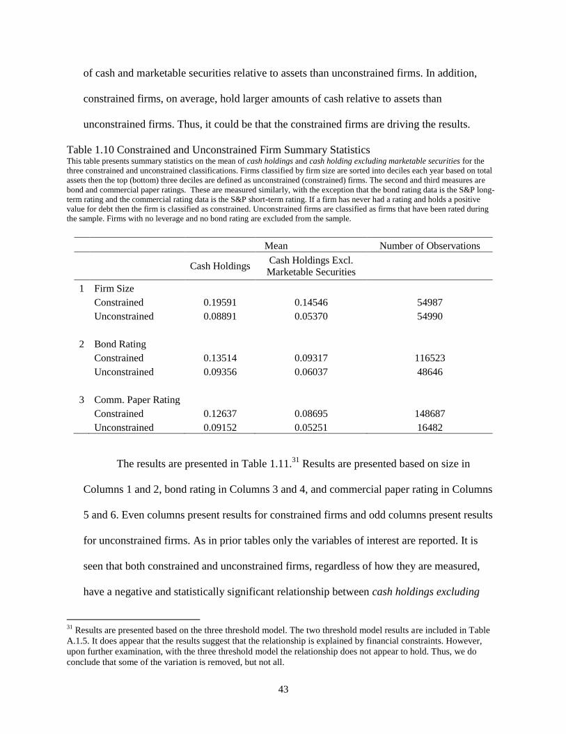
43

of cash and marketable securities relative to assets than unconstrained firms. In addition,

constrained firms, on average, hold larger amounts of cash relative to assets than

unconstrained firms. Thus, it could be that the constrained firms are driving the results.

Table 1.10 Constrained and Unconstrained Firm Summary Statistics This table presents summary statistics on the mean of cash holdings and cash holding excluding marketable securities for the

three constrained and unconstrained classifications. Firms classified by firm size are sorted into deciles each year based on total

assets then the top (bottom) three deciles are defined as unconstrained (constrained) firms. The second and third measures are

bond and commercial paper ratings. These are measured similarly, with the exception that the bond rating data is the S&P long-

term rating and the commercial rating data is the S&P short-term rating. If a firm has never had a rating and holds a positive

value for debt then the firm is classified as constrained. Unconstrained firms are classified as firms that have been rated during

the sample. Firms with no leverage and no bond rating are excluded from the sample.

Mean Number of Observations

Cash Holdings

Cash Holdings Excl.

Marketable Securities

1 Firm Size

Constrained 0.19591 0.14546 54987

Unconstrained 0.08891 0.05370 54990

2 Bond Rating

Constrained 0.13514 0.09317 116523

Unconstrained 0.09356 0.06037 48646

3 Comm. Paper Rating

Constrained 0.12637 0.08695 148687

Unconstrained 0.09152 0.05251 16482

The results are presented in Table 1.11.31

Results are presented based on size in

Columns 1 and 2, bond rating in Columns 3 and 4, and commercial paper rating in Columns

5 and 6. Even columns present results for constrained firms and odd columns present results

for unconstrained firms. As in prior tables only the variables of interest are reported. It is

seen that both constrained and unconstrained firms, regardless of how they are measured,

have a negative and statistically significant relationship between cash holdings excluding

31

Results are presented based on the three threshold model. The two threshold model results are included in Table

A.1.5. It does appear that the results suggest that the relationship is explained by financial constraints. However,

upon further examination, with the three threshold model the relationship does not appear to hold. Thus, we do

conclude that some of the variation is removed, but not all.

44

Table 1.11 Constrained and Unconstrained Firms Three Threshold Model This table presents the empirical results for the random effects threshold regressions of constrained and unconstrained firms. Cash Holdings excluding marketable securities is the

dependent variable in all regressions. Firms classified by firm size are sorted into deciles each year based on total assets then the top (bottom) three deciles are defined as

unconstrained (constrained) firms. The second and third measures are bond and commercial paper ratings. These are measured similarly, with the exception that the bond rating

data is the S&P long-term rating and the commercial rating data is the S&P short-term rating. If a firm has never had a rating and holds a positive value for debt then the firm is

classified as constrained. Unconstrained firms are classified as firms that have been rated during the sample. Firms with no leverage and no bond rating are excluded from the

sample. All other variables are included and defined in Tables 1.1 and 1.2. T-statistics are in parentheses and significance is denoted by * where the p-value is <.10, ** where the

p-value is <.05, and *** where the p-value is p<.01.

(1) (2)

(3) (4) (5) (6)

Size

Bond Rating

Commercial Paper Rating

Constrained Unconstrained Constrained Unconstrained Constrained Unconstrained

I(Interest Rate1 < γ1) 0.0165** 0.00973***

0.00481* 0.00547**

0.00281 0.0129***

(2.45) (4.79)

(1.67) (2.08)

(1.17) (3.77)

I(γ1 ≤ Interest Rate1 < γ2) -0.0543*** -0.000749

-0.0252*** -0.0172*

-0.0252*** -0.00498

(-2.76) (-0.12)

(-2.60) (-1.95)

(-3.26) (-0.38)

I(γ2 ≤ Interest Rate1 < γ3) 0.0268** -0.0202***

0.000928 -0.0109**

-0.00127 -0.0244***

(2.56) (-5.82)

(0.20) (-2.45)

(-0.33) (-4.30)


-0.3693*** -0.3071***

-0.3367*** -0.5792***

(-4.15) (-9.00)

(-5.20) (-6.68)

(-6.32) (-7.79)

Interest Rates in Lower Middle Region 1.1635*** -0.1219

0.3755* 0.2024

0.3359** -0.0202

(2.76) (-0.88)

(1.82) (1.08)

(2.04) (-0.07)

Interest Rates in Upper Middle Region -0.5481*** 0.1785***

-0.1857*** 0.0179

-0.1783*** 0.2382***

(-4.01) (3.61)

(-2.98) (0.29)

(-3.38) (3.00)


-0.1836*** -0.1530***

-0.1975*** -0.1286***

(-3.73) (-10.42)

(-9.52) (-7.11)

(-11.48) (-5.19)

N 44470 50970 100894 44507 130040 15361

Year Dummies No No

No No

No No


Yes Yes

Yes Yes


Yes Yes

Yes Yes

R2 0.46 0.583 0.462 0.542

0.467 0.585

45

marketable securities and the interest rate in the low and high regions. All results are

statistically significant at a 1% level. When looking at the lower middle region, the

constrained firms do have a positive and statistically significant relationship between cash

holdings excluding marketable securities and the interest rate. However, the unconstrained

firms do not show the expected negative relationship. When looking at rates in the upper

middle region, the relationship is reversed from what one would expect; the negative

relationship is found among the constrained firms and the positive relationship is found

amongst the unconstrained firms. Thus, when separating firms by financial constraints some

of the results are as expected, however it does not explain all the positive relationships found.

7.6 Alternative Explanations

In addition to the above explanations, three additional explanations are tested which

we do not report but do discuss.32

The first is that the positive relationship could be driven by

firms that are poorly governed. Dittmar and Mahrt-Smith (2007) find that poorly governed

firms do not efficiently manage cash balances and have a lower value of cash. Thus, these

poorly governed firms may not consider interest rates when deciding whether to hold cash. It

could be that these inefficient firms are driving the positive relationship between cash

holdings and interest rates.

The commonly used measures of corporate governance are the Gompers, Ishii,

and Metrick (2003) (GIM) index and the Bebchuk, Ishii, and Metrick (2003) (E) index. The

GIM index is available from Risk Metrics and measures the number of antitakeover

provisions a firm has. The E index is available on Lucian Bebchuk’s website and uses six

antitakeover provisions that Bebchuk, et al. (2003) have shown have the greatest impact on

32

All results are available upon request.

46

firm value.33

The variables are reported approximately every two to three years (1990, 1993,

1995, 1998, etc). Similar to prior literature, we assume that the index remains unchanged

during the unreported years. There are two restrictions when using the above indexes. The

first is that they are only available from 1990-2006. Thus, we are restricted to only testing for

the relationship between cash holdings and interest rates during this time. Second, the data

only cover S&P 1500 firms. Thus, the data set is substantially reduced.34, 35

To test whether poorly governed firms are driving the positive relationship, the data is

split into poorly governed firms and well governed firms. Firms are sorted into terciles each

year. Poorly governed firms are defined as the highest tercile of firms and well governed

firms are defined as the lowest tercile of firms. Very few of the relationships are statistically

significant. Furthermore, those relationships that are significant exist among poorly governed

firms which was not as predicted.

The second explanation tested is that some may argue that the relationship between

interest rates and cash holdings is not clear, and can be affected by other factors such as the

economy, which previous theories did not take into account. While it is true that interest rates

tend to be lower during weak economic times, we test the argument that firms build up cash

reserves when the economy is doing well and use cash during these weak economic times

when external capital might be more constrained. In Figure 1.2, it is shown that during

interest rate declines, the mean and median cash holdings ratios typically increase. This

suggests that firms start to hold more cash during the declining rates and conditions. Kahle

33

Data can be found at www.law.harvard.edu/faculty/bebchuk/data.shtml. 34

Due to the reduced number of observations, the results are presented for all firms and not split into mature and

growth firms. 35

Prior to splitting the sample into well and poorly-governed firms, the regressions are repeated with the smaller set

of firms. Results similar to the ones presented in the paper are not found. Specifically, the relationship in the high

region in both the two and three threshold models is insignificant for both measured of governance.

47

and Stulz (2013) document a decline in cash holdings during the start of the most recent

financial crisis followed by an increase in cash holdings to pre-crisis levels. In addition, they

find an increase in cash holdings to levels above pre-crisis levels for bank dependent firms

that is not due to a cut in capital expenditures. Thus, we repeat the regressions and include a

recession dummy variable that equals one if the National Bureau of Economic Research

reported the economy as being in a recession during that year and zero otherwise. The

dummy variable is interacted with all the prior interest rate variables. It is found that cash

holdings excluding marketable securities has a negative relationship with interest rates in the

middle region during recessions and a positive relationship during times when the recession

dummy is equal to zero. Thus, recessions are not to blame for the positive relationship.

The final explanation is that high-tech firms are driving the results. Zhou (2009)

found that the documented increase in cash holdings is among high-tech firms and that non-

high tech firms’ cash holdings remain relatively stable over 1980-2007. Zhou follows Brown,

et al. (2009) and defines a high-tech industry by the following 3-digit SIC codes: drugs (SIC

283), office and computing equipment (SIC 357), communications equipment (SIC 366),

electronic components (SIC 367), scientific instruments (SIC 382), medical instrument (SIC

384), and software (SIC 737).36

The baseline regressions are repeated excluding these high

tech industries. Results remain similar with the exception that the significance is removed

between the interest rate and cash holdings excluding marketable securities in the middle and

lower middle region across all data sets.

36

Brown, et al. (2009) use the definition provided by the United States Department of Commerce for high-tech

firms. This definition can be found at: “An Assessment of United States Competitiveness in High-Technology

Industries,” United States Department of Commerce, February 1983.

48

8. Quantile Regression

In further tests, results are presented based on quantile regressions. Whereas most

regressions estimate based on the conditional mean of the response variables, the quantile

regressions allows one to estimate the data at either the median or other quantiles of the

response variable. The advantage to using the quantile regression is that it is robust against

outliers in the data. It is also useful in estimating a relationship between variables in cases

where no or a weak relationship exists to see if differing relationships exist among different

ranges of the dependent variable.

The final results presented are based on the quantile regressions for the threshold

models.37

It is of interest to see if firms holding cash in a particular range are driving the

results. The quantile regression is also useful because cash holdings is highly skewed to the

right.38

We estimate the three threshold model at nine quantiles, namely the 10th

, 20th

, 30th

,

40th

, 50th

, 60th

, 70th

, 80th

, and 90th

. All control variables are included from the threshold

regressions including the industry dummies. However, the Mundlak (1978) and Chamberlain

(1980) devices are not included.

Results are presented in Table 1.12. For brevity, only the marginal effects for each

data set is presented. Columns 1-9 detail the relationship based on the nine quantiles. Results

in the first column referred to firms with lower cash holdings excluding marketable securities

and the level rises until quantile 90, which represents the highest level. Panel A presents the

results for the entire data set, Panel B and Panel C present results for mature and growth

firms, respectively.

37

In unreported regressions, the quantile regressions are run with just interest rate1. It is found that across all three

models interest rate1 is negatively and significantly related to cash holdings excluding cash equivalents at a 1%

level. 38

Across the entire data set, the 10th

percentile of cash holdings excluding marketable securities is 0.00514, the 50th

percentile is 0.04041, and the 90th

percentile is 0.27116.

49

In Panel A, interest rates in the lower region are significantly related to cash holding

excluding marketable securities across all quantiles of cash holdings. This does support the

finding that when interest rates are at extremely low levels all firms hold more cash. When

looking at the lower middle region, which is where the positive relationship was found, firms

with lower levels of cash holdings excluding marketable securities (quantiles 10-50) have a

positive relationship between cash holdings and interest rates. The coefficient declines in

value as we move across quantiles, becoming negative and statistically significant for firms

with the highest level of cash holdings (quantiles 80 and 90). Thus, firms with high cash

holdings are not driving the positive relationship between cash holdings excluding

marketable securities and interest rates, which supports the story we found when removing

zero-leverage firms and high tech firms in Sections 7.4 and 7.6, respectively. When looking

at the interest rates in the upper middle region, we again observe that firms in the lower

quantiles of cash holdings have a positive relationship between cash holdings excluding

marketable securities and interest rate1. The relationship does become negative and

statistically significant at upper quantiles of cash holdings. Finally, rates in the highest region

have a negative and statistically significant relationship between cash holdings excluding

marketable securities and interest rate1 amongst all quantiles. This relationship increases in

magnitude across the differing quantiles of cash. Panels B and C tell similar stories with

lower quantiles driving the positive relationship between cash holdings excluding marketable

securities and interest rate1.

In conclusion, it is found that firms with less cash holdings are driving the positive

relationship. This is not unexpected as firms with limited amounts of cash might not hold it

based on interest rates, but might be spending it based on firm-specific needs.

50

Table 1.12 Quantile Regression This table presents the empirical results for the quantile regressions of all firms. Cash Holdings excluding marketable securities is the dependent variable in all regressions. T-

statistics are in parentheses and significance is denoted by * where the p-value is <.10, ** where the p-value is <.05, and *** where the p-value is p<.01.

Panel A: All Firms

(1) (2) (3) (4) (5) (6) (7) (8) (9)

10 20 30 40 50 60 70 80 90

Interest Rates in Low Region -0.0008*** -0.0014*** -0.0021*** -0.0025*** -0.0028*** -0.003*** -0.003*** -0.003*** -0.002***

(-7.43) (-8.96) (-12.25) (-12.64) (-12.79) (-10.08) (-8.14) (-5.70) (-2.62)

Interest Rates in Lower Middle Region 0.0021*** 0.0033*** 0.0029*** 0.0025*** 0.00119** 0.00027 -0.0021** -0.004*** -0.009***

(6.79) (8.98) (7.47) (5.78) (2.20) (0.40) (-2.48) (-2.65) (-3.19)

Interest Rates in Upper Middle Region 0.0009*** 0.0008*** 0.0007*** 0.0004*** 0.00001 -0.0004** -0.001*** -0.003*** -0.005***

(8.47) (7.57) (6.02) (2.89) (0.09) (-2.12) (-5.25) (-8.13) (-7.77)

Interest Rates in High Region -0.0001*** -0.0002*** -0.0002*** -0.0003*** -0.0004*** -0.001*** -0.001*** -0.001*** -0.002***

(-4.10) (-4.97) (-6.44) (-7.53) (-8.54) (-9.81) (-10.55) (-11.63) (-12.44)

N 161103 161103 161103 161103 161103 161103 161103 161103 161103


(1) (2) (3) (4) (5) (6) (7) (8) (9)

10 20 30 40 50 60 70 80 90

Interest Rates in Low Region -0.00046** -0.0009*** -0.0016*** -0.0018*** -0.0022*** -0.002*** -0.002*** -0.00168* -0.00093

(-2.52) (-3.71) (-5.78) (-5.12) (-5.66) (-3.68) (-3.25) (-1.76) (-0.49)

Interest Rates in Lower Middle Region 0.0019*** 0.0033*** 0.0031*** 0.0030*** 0.0027*** 0.00093 0.00041 -0.00328 -0.00587

(3.26) (4.87) (4.23) (4.13) (2.78) (0.76) (0.23) (-1.01) (-1.24)

Interest Rates in Upper Middle Region 0.0010*** 0.0009*** 0.0007*** 0.00041* 0.00001 -0.00045 -0.002*** -0.003*** -0.006***

(5.28) (4.70) (3.26) (1.92) (0.03) (-1.50) (-3.15) (-3.64) (-4.24)

Interest Rates in High Region -0.0000598 -0.0000541 -0.0000213 -0.000118 -0.0002*** -0.000*** -0.001*** -0.001*** -0.003***

(-0.88) (-0.80) (-0.32) (-1.59) (-2.73) (-3.39) (-4.39) (-7.03) (-6.16)

N 48416 48416 48416 48416 48416 48416 48416 48416 48416

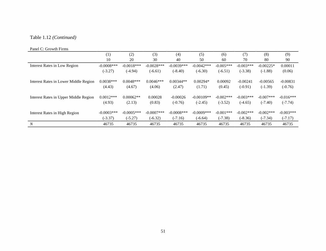
51



(1) (2) (3) (4) (5) (6) (7) (8) (9)

10 20 30 40 50 60 70 80 90

Interest Rates in Low Region -0.0008*** -0.0018*** -0.0028*** -0.0039*** -0.0042*** -0.005*** -0.003*** -0.00225* 0.00011

(-3.27) (-4.94) (-6.61) (-8.40) (-6.30) (-6.51) (-3.38) (-1.88) (0.06)

Interest Rates in Lower Middle Region 0.0038*** 0.0048*** 0.0046*** 0.00344** 0.00294* 0.00092 -0.00241 -0.00565 -0.00831

(4.43) (4.67) (4.06) (2.47) (1.71) (0.45) (-0.91) (-1.39) (-0.76)

Interest Rates in Upper Middle Region 0.0012*** 0.00062** 0.00028 -0.00026 -0.00109** -0.002*** -0.003*** -0.007*** -0.016***

(4.93) (2.13) (0.83) (-0.76) (-2.45) (-3.52) (-4.65) (-7.40) (-7.74)

Interest Rates in High Region -0.0003*** -0.0005*** -0.0007*** -0.0008*** -0.0009*** -0.001*** -0.002*** -0.002*** -0.003***

(-3.37) (-5.27) (-6.32) (-7.16) (-6.64) (-7.38) (-8.36) (-7.34) (-7.17)

N 46735 46735 46735 46735 46735 46735 46735 46735 46735

52

9. Conclusion

This paper examines the relationship between cash holdings and interest rates as

measured by the Treasury Constant Maturity Rate. To test the relationship, a random effects

threshold model is used and tested over multiple thresholds. In addition, the relationship is

tested not just over the entire population of firms available from Compustat but also for

mature and growth firms. The idea is that the cash holdings practices of these particular

groups may differ from the entire population of firms.

When using a cash holdings variable that contains cash and marketable securities, a

positive relationship between interest rates and cash holdings exists within most threshold

groups. To test whether the positive relationship is driven by the relationship between the

cash equivalent investments and interest rates, a new cash holdings variable is used that

includes cash, but not marketable securities. After using the new definition of cash holdings,

several positive relationships still exist between cash holdings and interest rates particularly

during the 1990’s.

To examine what is driving this positive relationship, several alternative explanations

are tested: the tax-based explanation, the cash flow hypothesis, pension fund contributions,

zero-leverage firms, financially constrained and unconstrained firms, firm governance,

recessions, and high-tech firms. After dividing the data sets into domestic and multinational

companies, the positive relationship is found for domestic firms. Thus, the tax-based

explanation does not explain the relationship and additional explanations are tested. Next,

operating and investing cash flows are included, but we find including them does not remove

the positive relationship. After including pension expense as an explanatory variable, the

positive relationship is still unaffected. It is found that zero-leverage firms and high-tech

53

firms hold large amounts of cash; after omitting these firms separately from the data sets the

positive relationship continues to hold. After dividing the data up into financially constrained

and unconstrained firms based on three separate measures, the positive relationship still

exists. Lastly, the positive relationship is shown not to hold for poorly governed firms, and it

cannot be explained by recessions. Thus, none of the explanations provided are able to

explain why a negative relationship does not exist. Finally, quantile regressions find that

firms in lower quantiles of cash holdings are driving the positive relationship between cash

and interest rates.

In conclusion, we find a positive relationship between cash holdings and interest

rates. Several explanations are examined, but none can completely remove the positive

relationship between interest rates and cash holdings. We conclude that the relationship is

driven by firms with lower levels of quantiles of cash holdings that are not considered

financially constrained as well as several factors that we are unable to test for and that there

exists a puzzle among interest rates and cash holdings.

54

References

Almeida, H., Campello, M., Weisbach, M.S., 2004. The cash flow sensitivity of cash. J. Finance

59, 1777-1804.

Bai, J., Perron, P., 2003. Computation and analysis of multiple structural change models. J. Appl.

Econometrics 18, 1-22.

Bates, T.W., Kahle, K.M., Stulz, R.M., 2009. Why do US firms hold so much more cash than

they used to? J. Finance 64, 1985-2021.

Baumol, W.J., 1952. The transactions demand for cash: An inventory theoretic approach. Q. J.

Econ. 66, 545-556.

Bebchuk, L., Cohen, A., Ferrell, A., 2009. What matters in corporate governance? Rev. Finance

Stud. 22, 783-827.

Brown, J.R., Fazzari, S.M., Petersen, B.C., 2009. Financing innovation and growth: cash flow,

external equity, and the 1990s R&D boom. J. Finance 64, 151-185.

Campbell, J.L., Dhaliwal, D.S., Schwartz Jr., W.C., 2012. Financing constraints and the cost of

capital: Evidence from the funding of corporate pension plans. Rev. Finance Stud. 25,

868-912.

Chamberlain, G., 1980. Analysis of variance with qualitative data. Rev. Econometric Stud. 47,

225-238.

Dittmar, A., Mahrt-Smith, J., 2007. Corporate governance and the value of cash holdings. J.

Finance Econ. 83, 599-634.

Ferreira, M.A., Custodio, C., Raposo, C.C., 2005. Cash Holdings and Business Conditions

(February 2005). Available at SSRN: http://ssrn.com/abstract=608664

Foley, C.F., Hartzell, J.C., Titman, S., Twite, G., 2007. Why do firms hold so much cash? A tax-

based explanation. J. Finance Econ. 86, 579-607.

Garcia-Teruel, P.J., Martinez-Solano, P., 2008. On the determinants of SME cash holdings:

Evidence from Spain. J. Bus. Finance Account. 35, 127-149.

Gompers, P., Ishii, J., Metrick, A., 2003. Corporate governance and equity prices. Q. J. Econ.

118, 107-155.

55

Guney, Y., Ozkan, A., Ozkan, N., 2007. International evidence on the non-linear impact of

leverage on corporate cash holdings. J. Multinatl. Finance Manage. 17, 45-60.

Harford, J., 1999. Corporate cash reserves and acquisitions. J. Finance 54, 1969-1997.

Harford, J., Klasa, S., Maxwell, W.F., 2013. Refinancing risk and cash holdings. J. Finance,

forthcoming.

Kahle, K.M., Stulz, R.M., 2013. Access to capital, investment, and the financial crisis. J. Finance

Econ. 110, 280-299.

Keynes, J.M., 1936. The General Theory of Employment. In: Interest and Money. Harcourt

Brace,

London.

Lins, K.V., Servaes, H., Tufano, P., 2010. What drives corporate liquidity? An international

survey of cash holdings and lines of credit. J. Finance Econ. 98, 160-176.

McLean, R.D., 2011. Share issuance and cash savings. J. Finance Econ. 99, 693-715.

Meltzer, A.H., 1963. The demand for money: A cross-section study of business firms. Q. J.

Econ. 77, 405-422.

Miller, M.H., Orr, D., 1966. A model of the demand for money by firms. Q.J. Econ. 80, 413-435.

Mundlak, Y., 1978. On the pooling of time series and cross section data. Econometrica 46, 69-

85.

Opler, T., Pinkowitz, L., Stulz R., Williamson, R., 1999. The determinants and implications of

corporate cash holdings. J. Finance Econ. 52, 3-46.

Ozkan, A., Ozkan, N., 2004. Corporate cash holdings: An empirical investigation of UK

companies. J. Bank. Finance 28, 2103-2134.

Pinkowitz, L., Stulz, R.M., Williamson, R., 2012. Multinationals and the High Cash Holdings

Puzzle (May 21, 2012). Charles A. Dice Center Working Paper No. 2012-10; ECGI -

Finance Working Paper No. 334/2012. Available at SSRN:

http://ssrn.com/abstract=2064046

Rauh, J.D., 2006. Investment and financing constraints: Evidence from the funding of corporate

pension plans. J. Finance 61, 33-71.

Rauh, J.D., 2009. Risk shifting versus risk management: Investment policy in corporate pension

plans. Rev. Finance Stud. 22, 2687-2733.

56

Strebulaev, I.A., Yang, B., 2013. The mystery of zero-leverage firms. J. Finance Econ. 109, 1-

23.

Tobin, J., 1956. The interest-elasticity of transactions demand for cash. Rev. Econ. Stat. 38, 241-

247.

Zhou, J., 2009. Increase in Cash Holdings: Pervasive or Sector-Specific? Unpublished Working

Paper.

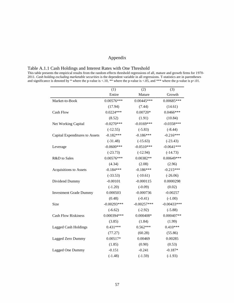
57

Appendix

Table A.1.1 Cash Holdings and Interest Rates with One Threshold This table presents the empirical results from the random effects threshold regressions of all, mature and growth firms for 1970-

2011. Cash holding excluding marketable securities is the dependent variable in all regressions. T-statistics are in parentheses

and significance is denoted by * where the p-value is <.10, ** where the p-value is <.05, and *** where the p-value is p<.01.

(1) (2) (3)

Entire

Mature

Growth

Market-to-Book 0.00576*** 0.00445*** 0.00685***

(17.94)

(7.44)

(14.61)

Cash Flow 0.0224***

0.00720*

0.0466***

(8.52)

(1.91)

(10.84)


-0.0169***

-0.0358***

(-12.55)

(-5.83)

(-8.44)


-0.186***

-0.216***

(-31.48)

(-15.63)

(-23.43)

Leverage -0.0600***

-0.0510***

-0.0641***

(-23.73)

(-12.94)

(-14.73)

R&D to Sales 0.00576***

0.00382**

0.00649***

(4.34)

(2.08)

(2.96)


-0.186***

-0.215***

(-33.53)

(-10.61)

(-26.06)


-0.000115

0.0000298

(-1.20)

(-0.09)

(0.02)


-0.000736

-0.00257

(0.48)

(-0.41)

(-1.00)

Size -0.00293***

-0.00257***

-0.00433***

(-6.62)

(-2.92)

(-5.88)


0.000408*

0.000407**

(3.85)

(1.84)

(1.99)


0.562***

0.410***

(77.27)

(60.28)

(55.86)


0.00469

0.00285

(1.85)

(0.90)

(0.53)


-0.241

-0.187*

(-1.48) (-1.59) (-1.93)

58

Table A.1.1 (Continued)

I(One-Yeart < γ1) 0.00644***

0.00964***

-0.00594*

(4.04)

(3.16)

(-1.73)


-0.2607***

-0.0648***

(-9.57)

(-5.70)

(-1.31)


-0.1592***

-0.2915***

(-15.32)

(-7.10)

(-11.29)

Constant 0.0748***

0.0417***

0.0714***

(7.40) (4.76)

(4.23)

N 161103

48416 46735

Year Dummies No

No

No


Yes

Yes


Yes

Yes

R2 0.529 0.538 0.491

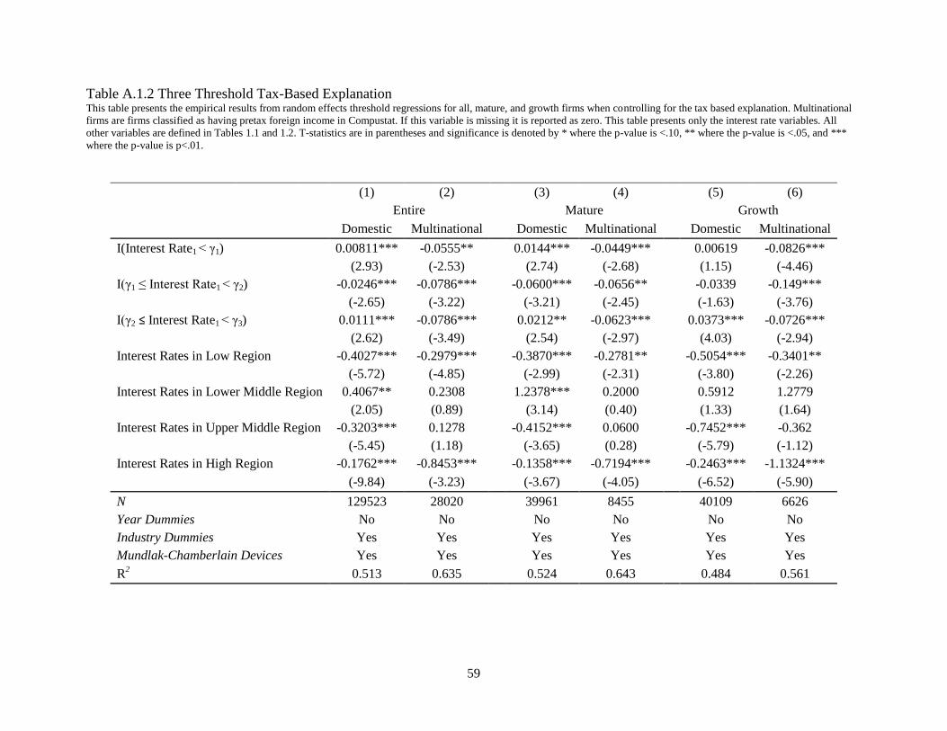
59

Table A.1.2 Three Threshold Tax-Based Explanation This table presents the empirical results from random effects threshold regressions for all, mature, and growth firms when controlling for the tax based explanation. Multinational

firms are firms classified as having pretax foreign income in Compustat. If this variable is missing it is reported as zero. This table presents only the interest rate variables. All

other variables are defined in Tables 1.1 and 1.2. T-statistics are in parentheses and significance is denoted by * where the p-value is <.10, ** where the p-value is <.05, and ***


(1) (2)

(3) (4) (5) (6)

Entire

Mature

Growth

Domestic Multinational Domestic Multinational Domestic Multinational

I(Interest Rate1 < γ1) 0.00811*** -0.0555**

0.0144*** -0.0449***

0.00619 -0.0826***

(2.93) (-2.53)

(2.74) (-2.68)

(1.15) (-4.46)

I(γ1 ≤ Interest Rate1 < γ2) -0.0246*** -0.0786***

-0.0600*** -0.0656**

-0.0339 -0.149***

(-2.65) (-3.22)

(-3.21) (-2.45)

(-1.63) (-3.76)

I(γ2 ≤ Interest Rate1 < γ3) 0.0111*** -0.0786***

0.0212** -0.0623***

0.0373*** -0.0726***

(2.62) (-3.49)

(2.54) (-2.97)

(4.03) (-2.94)


-0.3870*** -0.2781**

-0.5054*** -0.3401**

(-5.72) (-4.85)

(-2.99) (-2.31)

(-3.80) (-2.26)

Interest Rates in Lower Middle Region 0.4067** 0.2308

1.2378*** 0.2000

0.5912 1.2779

(2.05) (0.89)

(3.14) (0.40)

(1.33) (1.64)

Interest Rates in Upper Middle Region -0.3203*** 0.1278

-0.4152*** 0.0600

-0.7452*** -0.362

(-5.45) (1.18)

(-3.65) (0.28)

(-5.79) (-1.12)


-0.1358*** -0.7194***

-0.2463*** -1.1324***

(-9.84) (-3.23)

(-3.67) (-4.05)

(-6.52) (-5.90)

N 129523 28020 39961 8455 40109 6626

Year Dummies No No

No No

No No


Yes Yes

Yes Yes


Yes Yes

Yes Yes

R2 0.513 0.635 0.524 0.643 0.484 0.561

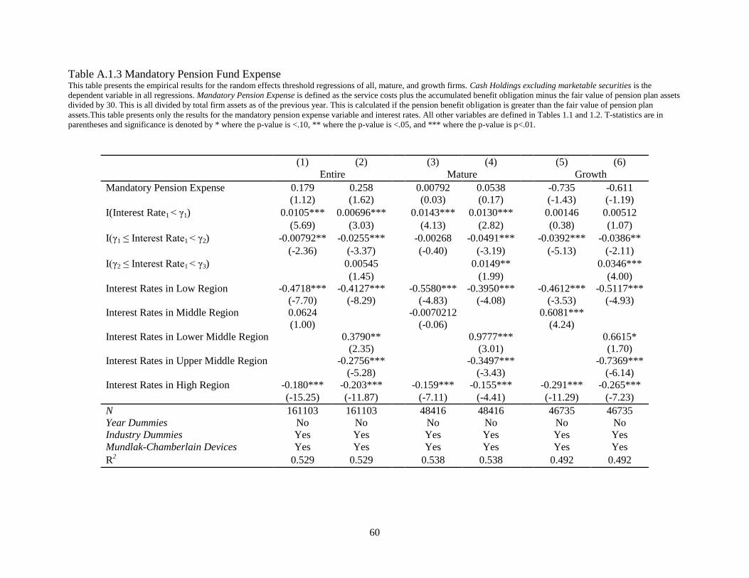
60

Table A.1.3 Mandatory Pension Fund Expense This table presents the empirical results for the random effects threshold regressions of all, mature, and growth firms. Cash Holdings excluding marketable securities is the

dependent variable in all regressions. Mandatory Pension Expense is defined as the service costs plus the accumulated benefit obligation minus the fair value of pension plan assets

divided by 30. This is all divided by total firm assets as of the previous year. This is calculated if the pension benefit obligation is greater than the fair value of pension plan

assets.This table presents only the results for the mandatory pension expense variable and interest rates. All other variables are defined in Tables 1.1 and 1.2. T-statistics are in


(1) (2) (3) (4) (5) (6)


Mandatory Pension Expense 0.179 0.258

0.00792 0.0538

-0.735 -0.611

(1.12) (1.62)

(0.03) (0.17)

(-1.43) (-1.19)

I(Interest Rate1 < γ1) 0.0105*** 0.00696***

0.0143*** 0.0130***

0.00146 0.00512

(5.69) (3.03)

(4.13) (2.82)

(0.38) (1.07)


-0.00268 -0.0491***

-0.0392*** -0.0386**

(-2.36) (-3.37)

(-0.40) (-3.19)

(-5.13) (-2.11)


0.00545

0.0149**

0.0346***

(1.45)

(1.99)

(4.00)


-0.5580*** -0.3950***

-0.4612*** -0.5117***

(-7.70) (-8.29)

(-4.83) (-4.08)

(-3.53) (-4.93)


-0.0070212

0.6081***

(1.00)

(-0.06)

(4.24)


0.3790**

0.9777***

0.6615*

(2.35)

(3.01)

(1.70)


-0.2756***

-0.3497***

-0.7369***

(-5.28)

(-3.43)

(-6.14)


-0.159*** -0.155***

-0.291*** -0.265***

(-15.25) (-11.87)

(-7.11) (-4.41)

(-11.29) (-7.23)

N 161103 161103 48416 48416 46735 46735

Year Dummies No No

No No

No No


Yes Yes

Yes Yes


Yes Yes

Yes Yes

R2 0.529 0.529

0.538 0.538

0.492 0.492

61

Table A.1.4 Cash Holdings of Zero-Leverage Firms This table presents the mean of Cash Holdings and Cash Holdings excluding marketable securities for the entire sample of zero-

leverage firms by year.

No Leverage Leverage > 0

Year

Number of

Observation

s

Cash

Holdings

Cash Holdings

Exc. Marketable

Securities

Number of

Observation

s

Cash

Holdings

Cash Holdings Exc.

Marketable

Securities

1970 52 0.23122 0.04871 943 0.06617 0.04130

1971 151 0.24803 0.07372 2286 0.08000 0.04673

1972 183 0.23902 0.07677 2465 0.08025 0.04540

1973 173 0.22509 0.06504 2650 0.07303 0.04087

1974 244 0.24338 0.10022 4106 0.07031 0.04349

1975 297 0.26776 0.10280 4221 0.07841 0.04796

1976 313 0.26349 0.10129 4236 0.08448 0.04829

1977 294 0.25863 0.10592 4195 0.08188 0.04748

1978 282 0.25691 0.09207 4098 0.07982 0.04340

1979 256 0.27892 0.10841 3924 0.07927 0.04054

1980 260 0.31086 0.10688 3784 0.08449 0.03991

1981 264 0.34096 0.08836 3552 0.09760 0.04057

1982 261 0.33826 0.09458 3393 0.09674 0.03926

1983 279 0.35833 0.09260 3231 0.11640 0.04404

1984 248 0.38416 0.09603 3104 0.11139 0.04260

1985 225 0.35565 0.10659 3070 0.10865 0.04282

1986 253 0.38018 0.12624 3049 0.11465 0.04522

1987 272 0.37630 0.14051 3078 0.11515 0.05278

1988 350 0.35818 0.21683 3927 0.10969 0.07580

1989 387 0.36149 0.23860 4248 0.10629 0.08293

1990 414 0.36073 0.23436 4373 0.10380 0.08286

1991 465 0.38675 0.26680 4529 0.11634 0.09005

1992 541 0.38367 0.25216 4706 0.12085 0.09056

1993 636 0.37704 0.23184 4877 0.12473 0.09084

1994 656 0.35682 0.21375 5058 0.11828 0.08463

1995 726 0.36174 0.23698 5527 0.12477 0.09147

1996 788 0.39182 0.26527 5619 0.14118 0.10451

1997 777 0.40022 0.26747 5427 0.13967 0.10192

1998 772 0.39055 0.26215 5414 0.14163 0.10705

1999 740 0.41346 0.28670 5355 0.14628 0.10828

2000 713 0.43051 0.29722 5081 0.14328 0.10526

2001 664 0.41500 0.28975 4676 0.14053 0.10406

2002 665 0.40862 0.27435 4375 0.14346 0.10860

2003 724 0.42608 0.30671 4123 0.15657 0.12199

2004 731 0.44188 0.29045 3945 0.16964 0.12514

2005 747 0.43641 0.27335 3740 0.16935 0.12574

2006 727 0.43992 0.28481 3574 0.16870 0.12612

62

Table A.1.4 (Continued)

2007 686 0.44479 0.30427 3398 0.16262 0.12312

2008 621 0.39919 0.30266 3297 0.14870 0.12131

2009 648 0.39028 0.29817 3184 0.16464 0.13347

2010 650 0.39631 0.29153 3043 0.16820 0.13661

2011 571 0.40551 0.29885 2734 0.15758 0.12821

63

Table A.1.5 Constrained and Unconstrained Firms with Two Thresholds This table presents the empirical results for the random effects threshold regressions of constrained and unconstrained firms. Cash Holdings excluding marketable securities is the

dependent variable in all regressions. Firms classified by firm size are sorted into deciles each year based on total assets then the top (bottom) three deciles are defined as

unconstrained (constrained) firms. The second and third measures are bond and commercial paper ratings. These are measured similarly, with the exception that the bond rating

data is the S&P long-term rating and the commercial rating data is the S&P short-term rating. If a firm has never had a rating and holds a positive value for debt then the firm is

classified as constrained. Unconstrained firms are classified as firms that have been rated during the sample. Firms with no leverage and no bond rating are excluded from the

sample. All other variables are included and defined in Tables 1.1 and 1.2. T-statistics are in parentheses and significance is denoted by * where the p-value is <.10, ** where the

p-value is <.05, and *** where the p-value is p<.01.

(1) (2)

(3) (4) (5) (6)

Size

Bond Rating

Commercial Paper Rating

Constrained Unconstrained Constrained Unconstrained Constrained Unconstrained

I(Interest Rate1 < γ1) 0.0133*** 0.0140***

0.00777*** 0.00991***

0.00730*** 0.0185***

(2.70) (8.40)

(3.18) (5.33)

(3.79) (6.41)

I(γ1 ≤ Interest Rate1 < γ2) -0.0235*** 0.00887***

-0.0111** -0.000364

-0.00970*** 0.00731

(-2.64) (3.04)

(-2.49) (-0.10)

(-2.78) (1.33)


-0.4247*** -0.3485***

-0.3750*** -0.7044***

(-2.77) (-8.90)

(-5.02) (-5.78)

(-5.77) (-8.28)

Interest Rates in Middle Region 0.4109** -0.2679***

0.119 -0.0716

0.0899 -0.2308**

(2.47) (-4.97)

(1.41) (-1.07)

(1.37) (-2.26)


-0.1652*** -0.1166***

-0.1638*** -0.0960***

(-6.16) (-11.89)

(-12.43) (-7.95)

(-13.95) (-5.05)

N 44470 50970 100894 44507 130040 15361

Year Dummies No No

No No

No No


Yes Yes

Yes Yes


Yes Yes

Yes Yes

R2 0.46 0.583

0.462 0.542

0.468 0.586

64

CHAPTER 2

Do Business Cycles Influence Corporate Cash Holdings?

1. Introduction

Corporate cash holdings have become a key discussion topic in the finance literature

in recent years and this attention has come at a time when companies are holdings record

amounts of cash. According to the Federal Reserve Flow of Funds, U.S. corporate cash

crossed the $2 trillion mark in the second quarter of 2011.39

As such, several theories have

arisen attempting to explain why companies in the U.S. and around the world are holding

more cash. One suggestion is that companies are holding larger stockpiles of cash for

precautionary measures. For example, Goldstein (2011) attributes the growth in cash

balances to the recent recession and financial crisis. While several academic papers assume

cash becomes increasingly important during recessions, few have shown this result.40

This

paper fills this gap by examining the relationship between business cycles and cash holdings.

Using panel data from 1976 until 2012, it is clear that corporate cash holdings show cyclical

patterns.41

More specifically, companies seem to hold more cash during weaker economic

times than stronger times. Upon further examination, we document that cash holdings

39

When using Federal Reserve Flow of Funds data, cash holdings is calculated as the level of nonfarm nonfinancial

business liquid assets divided by total assets. 40

Almeida, et al. (2004), Ferreira, et al. (2005), Baum, et al. (2006), and Duchin, et al. (2010), do examine corporate

cash holdings and business conditions which are discussed later in the paper. 41

With such a long observation period, we are able to analyze five US recessions: January 1980 - July 1980, July

1981 - November 1982, July 1990 - March 1991, March 2001 - November 2001, and December 2007 - June 2009.

65

initially decline during recessions and then increase. Interestingly, the most robust finding in

this paper is that corporate cash holdings increase around the time the National Bureau of

Economic Research (NBER) announces a recession. Thus, the relationship that most papers

expect between cash holdings and recessions seems to be a result of the average firm holding

cash due to the announcement of recessions.

The use of NBER recession dates differentiates this paper from the previous

literature.42

In addition to using the dates of actual recessions, we utilize the dates of the

announcement memos made by the NBER, which we will refer to as the announcement

dates. This is done because there can be a significant lag between when a recessions actually

begins and it is announced by the NBER. The lag is primarily due to the fact that the

information the NBER uses to make a determination regarding a recession is lagged as well.

Examining the previous five recessions, the average time between when a peak occurred and

when the peak was announced by the NBER is 8.4 months or close to three-quarters of a

year. While it can be argued that companies are aware of a recession prior to the

announcement, we suggest that companies value the confirmation made by experts at the

NBER. Companies respond to this confirmation by holding elevated levels of cash because

they might not be able to fully access capital when it is needed during a recession.

Figure 2.1, which plots cash as a percentage of corporate assets from January 1976 to

December 2013, provides support that using recessionary dates and announcement dates

yield differing results. The graph reports both the mean and median measure of cash

holdings, which is obtained by using all non-missing observations in Compustat. Panel A

42

The common macroeconomic variables used in the previous literature to indicate recessions are analyzed here as

well.

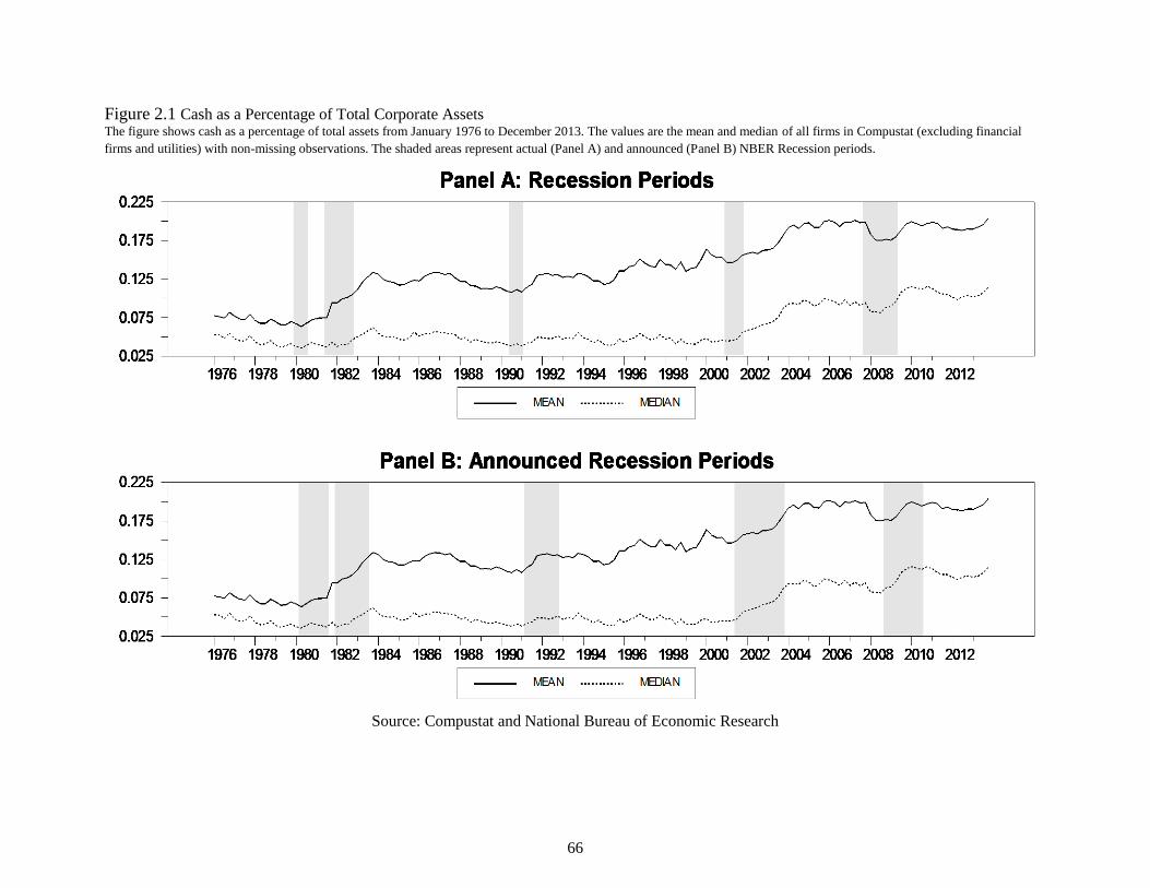
66

Figure 2.1 Cash as a Percentage of Total Corporate Assets The figure shows cash as a percentage of total assets from January 1976 to December 2013. The values are the mean and median of all firms in Compustat (excluding financial

firms and utilities) with non-missing observations. The shaded areas represent actual (Panel A) and announced (Panel B) NBER Recession periods.

Source: Compustat and National Bureau of Economic Research

67

shades the actual recession periods as determined by the NBER while panel B shades the

dates between when the NBER announced a peak and when it announced a trough.

Panel A of Figure 2.1 shows that troughs in both the mean and median measure of

cash holdings occur during recessions, the 1982 recession being the lone exception. Panel B

shows that both the mean and median measures of cash holdings increase at the

announcement of a peak. Specifically, most of the series seem to increase during the quarter

an announcement is made, regardless of the lag in time between when the recession began

and the announcement. Another thing to notice in Figure 2.1 is that with the exception of the

most recent recession, cash holdings increase to levels greater than those prior to the

recession. During the most recent recession, cash holdings increased to its pre-crisis level.

This post-recession increase possibly indicates that companies were not just holding cash

because of the recession but that the recession changed the holdings strategies of companies.

This paper adds to the literature by documenting a relationship between cash holdings

and business cycles. As mentioned, few papers show this relationship, and those that do use

data sets of all firms and one or two macroeconomic indicators. In this analysis, three

different measures of recessions are used: several common macroeconomic indicators, the

NBER actual recession dates, and the NBER announced recession dates. Initially, these

methods seem similar, however, using the dates provided by the NBER, we show that

companies tend to use cash reserves during the initial stages of recessions but then respond to

the announcement of recessions by increasing cash holdings. The fact that companies react in

this manner after an announced recession is in conflict with the precautionary cash holdings

theory. In other words, companies are not holding larger amounts of cash in preparation for a

recession, but are holding larger amounts of cash once they know the economy is in a

68

recession. This suggests that the macroeconomic indicators used in past papers may not be

providing a complete view of the reason companies hold cash during recessions.

It is believed that due to the differing nature of mature and growth firms, recessions

might affect their cash holdings practices differently. Thus, in addition to having a data set

that includes all companies in Compustat with non-missing variables, companies are split up

into mature and growth firms. We document that the cash holdings of both groups do decline

during a recession and increase during announced recessions, but both the decline and the

increase in cash holdings are greater for growth firms. Furthermore, the effect is also

examined for constrained and unconstrained firms. While the previous literature has studied

constrained and unconstrained firms in the context of business cycles and cash holdings, no

one has documented the announcement effect of recessions that is found in this paper. Using

several measures of financial constraints, an announcement effect is found for both

unconstrained and constrained firms during the quarter in which a recession is announced.

The remainder of the paper is organized as follows: Section 2 discusses relevant

literature surrounds cash holdings, Section 3 discusses the NBER recessions and

announcements in further detail, and Section 4 discusses the data used in this paper. Section

5 presents the econometric model. Section 6 presents the empirical results using the entire,

mature and growth data sets. Section 7 presents results when classifying firms as constrained

and unconstrained, and Section 8 concludes.

2. Literature Review

By using NBER reported recession dates, we offer a unique view of the relationship

between cash holdings and business conditions. Past literature has represented recessionary

69

periods using macroeconomic indicators. However, these macroeconomic indicators may not

capture the entire reaction of companies’ cash balances during recessionary periods.

Almeida, et al. (2004) showed that constrained firms’ cash holdings increase when cash

flows are higher. Therefore, the sensitivity of cash is positive. They were able to relate this to

business cycles and found that constrained firms increase their holdings of cash following

negative macroeconomic shocks.43

Ferreira, et al. (2005) examined business conditions as a

determinant of firms’ cash holdings and found evidence that cash levels increase during

recessions, especially for financially constrained firms.44

Baum, et al. (2006) employed the

GARCH model and used macroeconomic aggregates to show that over time there is variation

in a firm’s cash-to-assets ratio. They also documented that a doubling of uncertainty in the

economy led to a reduction in the dispersion of the cash-to-assets ratio between 8% and 40%.

Duchin, et al. (2010) studied the 2007 financial crisis and documented that corporate

investment decline is greatest for firms that have low cash reserves, are financially

constrained, or operate in industries dependent on external finance. They also found that cash

had an insignificant effect from July 2008 to March 2009 due to firms’ financial power

evolving as the crisis lengthened. Kahle and Stulz (2013) document a decline in cash

holdings during the most recent financial crisis followed by an increase in cash holdings to

pre-crisis levels. In addition, they find an increase in cash holdings to levels above pre-crisis

levels for bank dependent firms that is not due to a cut in capital expenditures. They also find

that the increase in cash holdings is not due to drawdowns of credit lines in 2008. This last

finding contradicts recent evidence by Ivanshina and Scharfstein (2010). Our paper expands

43

Almeida, et al. (2004) measure macroeconomic shocks as the log of real GDP and three of its lags. 44

Ferreira, et al.(2005) use the one-year equity market return, relative Treasury bills rate of return, term spread, and

default spread as macroeconomic indicators.

70

upon this finding by documenting an announcement effect in cash holdings following NBER

recession announcements that accounts for the increase in cash holdings.

Four motives explaining why companies hold cash have been identified in the

literature. These motives are- the precautionary motive, the transaction motive, the tax

motive, and the agency motive.45

This paper focuses on the precautionary motive. The

precautionary motive was first related to cash holdings by Keynes (1936) who hypothesized

that firms hold cash to protect themselves against future unknown events. Recently, several

papers have investigated the precautionary motive with mixed results. Han and Qiu (2007)

found a positive relationship between cash flow volatility and cash holdings among

financially constrained firms, thus finding support for the precautionary motive. Lins et al.

(2010) survey Chief Financial Officers (CFOs) in 29 countries to measure corporate liquidity

around the world. They did not find support for the precautionary motive related to non-

operational cash and claimed that cash is held to guard against future shocks during bad

times. They found that lines of credit are used as a precautionary motive because they are

held to fund growth opportunities while cash is held for insurance. Von Eije (2012)

documented that listed firms hold cash for precautionary reasons.

As a brief literature review, we want to discuss several cornerstone papers in the cash

holdings literature as control variables are derived from these papers. The most extensive

work has addressed balance sheet determinants and corporate cash holdings. Opler, et al.

(1999) documented that firms with strong growth opportunities and riskier activities hold

relatively more cash. They also found that large firms and those with credit ratings tend to

hold relatively less cash. Mikkelson and Partch (2003) showed that firms with cash holdings

of more than 25% of their assets support growth and have a median operating performance

45

See Bates et al. (2009) for a summary of these motives.

71

that is greater than the performance of firms matched by size and industry, and thus found no

evidence that large cash holdings hurt firm performance. Bates, et al. (2009) documented that

from 1980 to 2006, U.S. firms increased cash holdings. They found increases among firms

that either do not pay dividends, are in more recent IPO listing cohorts, or are in industries

that experience the greatest increase in idiosyncratic volatility. Reasons attributed to this

build-up are fallen inventories, increased cash flow risk, decreased capital expenditures, and

increased R&D expenditures. Brown and Petersen (2011) showed a strong link between

R&D smoothing and cash holdings during the 1998-2000 boom and the 2000-2002 bust.

Harford (1999) showed that cash-rich firms are more likely to make acquisitions.

Furthermore, he found that these acquisitions decrease firm value. While this paper does not

focus solely on cash rich firms, we find evidence for both mature and growth firms that

having more acquisitions lowers the amount of cash a company will hold. Colquitt, et al.

(1999) document the differences in cash holdings across property-liability issuers and find

that cash holdings are smaller for larger insurers and financially stronger insurers. Campello,

et al. (2010) surveyed CFOs in 39 countries in December 2008, during the middle of the most

recent financial crisis, and found that financially constrained firms planned to cut more

investment, technology, marketing, and employment relative to financially unconstrained

firms. Furthermore, constrained firms had to use cash reserves and cut planned dividends

during the crisis. Fresard (2010) provided a link between firms’ cash holdings and future

market performance. He found that firms with large cash reserves are able to strategically

position themselves at the expense of industry rivals.

72

3. NBER Recessions

As mentioned in the introduction, we use NBER recession dates and announcements

of recessions in addition to several common macroeconomic indicators. In this section, we

discuss more about these dates and the reasoning behind using them.

The NBER provides the dates of the peaks and troughs in the business cycle from

1854 until 2009.46

Since 1978, these dates have been determined by the NBER’s Business

Cycle Dating Committee, which is comprised of academics and directors of programs that

are related to business cycle research. The committee uses measures that capture both the

broad economy and a variety of specific sectors to determine troughs and peaks. Since the

indicators are on a lagged release, the committee determines the start of a recession after it

has occurred. They also define a recession as a significant decline in several economic

performance measures lasting more than a few months. This broad definition allows the

committee to take ample time to determine whether there was a sustained decline in the

economy or a mild dip. Table 2.1 provides a detailed list of the month and year that the

dating committee has determined was a start (peak) and end (trough) of a recessionary

period. While most recessions have lasted for less than a year, the most recent recession and

the recession in 1981-1982 lasted for 18 and 16 months, respectively making them the

longest recessions in United States history.

Once the dating committee determines a peak or trough has occurred, an official

announcement is released. Official announcements have only been made since the formation

of the dating committee in 1978. All past announcements are posted on the NBER’s website.

Table 2.1 also lists the dates on which an announcement was made regarding both peaks and

46

This information can be found at: http://www.nber.org/cycles/cyclesmain.html.

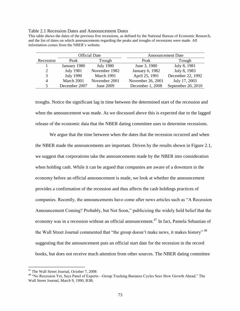
73

Table 2.1 Recession Dates and Announcement Dates This table shows the dates of the previous five recessions, as defined by the National Bureau of Economic Research,

and the list of dates on which announcements regarding the peaks and troughs of recessions were made. All

information comes from the NBER’s website.

Official Date

Announcement Date

Recession Peak Trough Peak Trough

1 January 1980 July 1980

June 3, 1980 July 8, 1981

2 July 1981 November 1982

January 6, 1982 July 8, 1983

3 July 1990 March 1991

April 25, 1991 December 22, 1992

4 March 2001 November 2001

November 26, 2001 July 17, 2003

5 December 2007 June 2009

December 1, 2008 September 20, 2010

troughs. Notice the significant lag in time between the determined start of the recession and

when the announcement was made. As we discussed above this is expected due to the lagged

release of the economic data that the NBER dating committee uses to determine recessions.

We argue that the time between when the dates that the recession occurred and when

the NBER made the announcements are important. Driven by the results shown in Figure 2.1,

we suggest that corporations take the announcements made by the NBER into consideration

when holding cash. While it can be argued that companies are aware of a downturn in the

economy before an official announcement is made, we look at whether the announcement

provides a confirmation of the recession and thus affects the cash holdings practices of

companies. Recently, the announcements have come after news articles such as “A Recession

Announcement Coming? Probably, but Not Soon,” publicizing the widely held belief that the

economy was in a recession without an official announcement.47

In fact, Pamela Sebastian of

the Wall Street Journal commented that “the group doesn’t make news, it makes history” 48

suggesting that the announcement puts an official start date for the recession in the record

books, but does not receive much attention from other sources. The NBER dating committee

47

The Wall Street Journal, October 7, 2008 48

“No Recession Yet, Says Panel of Experts—Group Tracking Business Cycles Sees Slow Growth Ahead,” The

Wall Street Journal, March 9, 1990, B3B.

74

Chairman Robert E. Hall has even said that stories about the group’s decisions “have never

occurred closer to the front of The Wall Street Journal than page 14.”48

However, we show

that regardless of whether companies directly react to the announcement or react to the

tightening of credit conditions brought on by the announcement, that companies hold larger

amounts of cash after an announcement is made.

We are in no way suggesting that companies cash holdings practices are not altered

before the official announcement; in fact, we find that companies have a strong decline in

cash holdings prior to an announcement. This decline in cash suggests that the companies use

capital resources to fund projects during this time which might be an indicator of a weak

lending environment and thus another sign that the economy could be in a recession.

With all this evidence, going forth we examine not just the dates that the economy has

been determined to be in a recession, but also use the range of dates between when the NBER

made an announcement of a peak and a trough. As evident in Figure 2.1, we find that using

these two dates provides results that are contrary to the precautionary cash holdings theory

and instead find an announcement effect for cash holdings.

4. Data

In this section, the creation of the three main data sets is discussed. In addition, the

corporate control variables and the macroeconomic variables are discussed. The summary

statistics for all data sets and variables are also presented.

4.1 Data Sets and Corporate Control Variables

The accounting data comes from Compustat Quarterly files. While the dating

committee provides the month in which the peak or trough occurs, we are limited to either

75

using yearly are quarterly data due required reporting. Quarterly data is preferred to annual

data as to more accurately define a period as being in a recession and thus quarterly data is

used. The sample is restricted to firms headquartered within the United States, firms with

positive values for total assets and sales, and firms with non-missing values for all variables.

In addition, financial firms (SIC 6000-6999) and utilities (SIC 4900-4999) are excluded

because they are regulated: financial firms hold cash for business practices and utilities hold

cash for regulatory purposes. All continuous variables are winsorized at a 1% level.

This paper uses several distinctly different panel data sets covering 1976 through

2012 to examine recessionary cash holdings practices.49

The first covers the entire sample of

publicly traded firms that meet the above restrictions. The data set covering all public firms

contains 477,304 firm-quarter observations. Due to the differences in policies between

mature and growth firms, two additional data sets are created to examine the potential

differences in cash management polices during business cycles. To create these data sets, we

rank firms into deciles based on the one-year growth rate in sales each quarter.50

The bottom

three deciles of firms are defined as mature firms. The data set of mature firms consists of

126,243 firm-quarter observations. The top three deciles of firms are defined as growth firms.

The growth firm data set contains 126,246 firm-quarter observations. In all data sets, firms

are allowed to enter and leave the panel.

The corporate control variables that have been chosen are in line with past literature

such as in Opler, et al. (1999). We control for a firm’s market-to-book rating, cash flow, net

49

Quarterly data becomes comprehensive beginning in 1975. Thus, our data set begins in 1976 to accommodate

creating the mature and growth data sets. 50

Additionally, firms were ranked based on the five-year growth rate in sales. While this restricted the data set to the

years 1980-2012, and the mature and growth data sets to 73,655 and 73,664 observations, respectively, the results

were similar. The growth rate in the number of employees was also used to calculate mature and growth firms and

the results remain similar. These results are available upon request.

76

working capital to assets, capital expenditure to assets, leverage, R&D to sales, acquisitions

to assets, dividends, investment grade rating, firm size, and the standard deviation of cash

flows.51

Capital expenditures and acquisitions are reported on a year-to-date basis in

Compustat. To arrive at quarterly observations, the data is lagged one quarter and the lagged

value is subtracted from the current quarterly observation for quarters 2, 3, and 4. All

variables are defined in appendix Table A.2.1.

4.2 Variables to Capture Business Cycles

The variables used to define business cycles and the dummy variables used to define

recession periods are defined below.

4.2.1 Macroeconomic Variables

The NBER defines a recession as a “significant decline in economic activity spread

across the economy, lasting more than a few months, normally visible in real GDP, real

income, employment, industrial production, and wholesale-retail sales.”52

Several

macroeconomic variables are examined in this paper and are chosen based on the above

definition and common variables shown in the literature to have business cycle variations.

We include a measure of employment, industrial production, and GDP as defined below.53

In

addition, the term spread and default spread are included because these have been shown to

have strong business cycle variations. The majority of the variables are obtained from the

Federal Reserve Economic Data (FRED) unless otherwise noted. It is expected that the cash

51

We are aware that the bond rating data is comprehensively collected by Compustat starting in 1985. The main

results do not change when this variable is excluded. 52

http://www.nber.org/cycles/cyclesmain.html 53

In previous versions, we included real personal income defined as the measure of consumer wages and income.

This variable was highly correlated with industrial production (correlation of .979 and statistically significant at a

1% level). Thus, real personal income is excluded from the regressions.

77

holdings of firms should vary inversely with the economy as measured by these common

economic indicators.

Employment is the civilian employment to population ratio. A decline in the employment

to population ratio is an indicator of an impending recession. As the employment ratio

declines, corporate cash holdings are expected to increase. Thus, a negative relationship is

expected between employment and cash holdings.

Industrial Production is an indexed measure of real production output of manufacturing,

mining, and utilities. It is believed that a sustained decrease in the index is an indicator that

the economy might be entering a recession. Companies are expected to increase holdings of

cash during a recession and thus a negative relationship is expected.

Gross Domestic Product (GDP) Gap is real GDP minus real potential GDP. Real GDP is

the final value of goods and services produced within a country in a given period of time.

Real potential GDP is published by the Congressional Budget Office (CBO) and is the

estimate of output the economy would produce with a high rate of use of its capital and labor

resources.54

As the economy nears economic turmoil the gap between the two will be

negative a larger magnitude represents a worsening economy. A positive gap is a sign that

the economy is in a stage of expansion and is growing faster than predicted. A negative

relationship is expected between GDP Gap and cash holdings.

Term Spread is defined as the difference between the ten-year and one-year Treasury

Constant Maturity Rate. Fama and French (1989) find that the term spread displays business

cycle patterns. Wheelock and Wohar (2009) provide a literature survey of the term spread

54

The CBO states that real potential GDP is “not a technical ceiling on output that cannot be exceeded. Rather, it is

a measure of maximum sustainable output…” Thus, a positive GDP Gap can be found which can also be associated

with increased inflationary pressure. There are 43 out of 148 quarters where a positive GDP Gap is found. More on

how the CBO measures potential GDP can be found at:

http://www.cbo.gov/sites/default/files/cbofiles/ftpdocs/30xx/doc3020/potentialoutput.pdf.

78

and its predictive power with output growth and recessions across several countries. While

we expect a negative relationship between cash holdings and the previous three

macroeconomic controls, the term spread increases during recessionary periods and declines

during expansions. Thus, a positive relationship is expected.

Default Spread is defined as the difference between Moody’s Aaa corporate bond yield

and Moody’s Baa corporate bond yield. Chen (1991) confirms that the default spread is

negatively correlated with output growth. Thus, a negative relationship is expected with cash

holdings.

To confirm the predicted relationships between cash holdings and the above

macroeconomic variables, graphs of all variables can be found in Figure 2.2. It is clear that

the civilian employment ratio, industrial production index, and GDP Gap decline during the

recessions. The term spread appears to increase across recessions. The default spread has a

less obvious relationship, increasing during some recessions and remaining stable during

other recessions. Figure 2.1 shows that cash holdings falls during the initial periods of

recession but then increases. Thus, confirming a negative relationship between employment,

industrial production, GDP Gap, and cash holdings. The positive relationship is found

between term spread and cash holdings. Given Figure 2.2, the relationship between default

spread and cash holdings seems to be less obvious.

4.2.2 Dummy Variables for Recessions and Announced Recessions

Dummy variables are used to examine the reaction of cash holdings during NBER-

defined recessions and during the periods between NBER announcements of recessions. By

79

Figure 2.2 Graphs of Common Economic Indicators and Recessions This figure contains five different measures of macroeconomic conditions from 1976 until 2012. Employment is the civilian employment to population ratio. Industrial Production

is an indexed measure of real production output of manufacturing, mining, and utilities. Gross Domestic Product (GDP) Gap is real GDP minus real potential GDP. Term Spread

is defined as the difference between the ten-year and one-year Treasury Constant Maturity Rate. Default Spread is defined as the difference between Moody’s Aaa corporate bond

yield and Moody’s Baa corporate bond yield. The shaded areas are recessions as defined by the NBER.

EMPLOYMENT

1980 1985 1990 1995 2000 2005 201056

57

58

59

60

61

62

63

64

65

TERMSPREAD

1980 1985 1990 1995 2000 2005 2010-2

-1

0

1

2

3

4

INDUSTPRODUCTION

1980 1985 1990 1995 2000 2005 201040

50

60

70

80

90

100

110

DEFAULTSPREAD

1980 1985 1990 1995 2000 2005 20100.5

1.0

1.5

2.0

2.5

3.0

3.5

GDPGAP

1980 1985 1990 1995 2000 2005 2010-1200

-1000

-800

-600

-400

-200

0

200

400

80

including the dummy variables, we are able to identify how cash holdings react during

economic downturns as opposed to the entire business cycle.

Recession Dummy is a dummy variable equal to one if the dates covered by the quarterly

report fall during a recession, as defined by the NBER, and zero otherwise. This measure

includes partial quarters. This variable will capture the change in cash during the five

recessions.

Announced Recession Dummy is a dummy variable equal to one if the dates covered by

the quarterly report fall during the period between recession announcements made by the

NBER and zero otherwise. This measure includes partial quarters. It is expected that the

announcement of a recession would reconfirm the declining economic indicators and

companies would thus react by holding more cash.

Whole Quarter Announced Recession Dummy is a dummy variable equal to one if the

dates covered by the quarterly report fall between recession announcements made by the

NBER and zero otherwise. Only quarters that are completely covered by the announced

recession period are included. This is used as a robustness check of the partial quarter

variable.

First Quarter Announced Recession is a dummy variable equal to one if the quarterly

report falls during the first quarter of an announced recession and zero otherwise. This

measure includes partial quarters and is to control for the response of firms when an

announcement has been made. This is a check of an announcement effect.

First Whole Quarter Announced Recession is a dummy variable equal to one if the

quarterly report falls during the first full quarter of an announced recession and zero

81

otherwise. This measure does not include partial quarters and is used as a robustness

measure.

4.3 Summary Statistics

Table 2.2 contains the summary statistics for the corporate control variables. Panel A

shows summary statistics for all firms and Panels B and C are for the mature and growth

firms, respectively. The average firm holds 14.53% of total assets as cash and marketable

securities. The average mature firm holds slightly more at 14.63% and the average growth

firm holds 18.22% of total assets as cash and marketable securities. Mature firms have a

lower market-to-book ratio than growth firms. As expected, growth firms have larger capital

expenditures to assets, R&D to sales, and acquisitions to assets than mature firms. Mature

firms have more leverage than growth firms. Around 20% of mature firm-year observations

pay a dividend and slightly less growth firm-year observations pay a dividend. More mature

firms have investment grade ratings than growth firms. The average mature firm is slightly

larger than the average growth firm suggesting that the growth firms are firms that are re-

entering the growth phase possibly after going through a mature phase.

Table 2.3 displays the summary statistics for the macroeconomic indicators as well as

the recession dummy variables.55

Panel A displays the summary statistics for the

macroeconomic indicators. An interesting feature of the summary statistics is that the mean

of the GDP gap is -161.0, which would seem to imply that on average the economy is below

potential GDP. This is deceiving however, because GDP gap is highly skewed to the right

55

Panel A displays statistics based on the 148 quarterly observations for the macroeconomic indicators. Panels B

and C present statistics based on the data set that contains all public firms. While the percentages do change for the

mature and growth firms, the changes are not dramatic. These statistics are available upon request.

82

Table 2.2 Summary Statistics for All, Mature, and Growth Firms This table represents the summary statistics on key variables for the 1976-2012 samples for all, mature and growth firms. Cash

holdings, the dependent variable, is defined as cash and marketable securities divided by total assets. Market-to-book ratio is

defined as the market value per share to the stated book value of equity. Cashflow is earnings after interest, dividends, and taxes

divided by total assets. Net working capital is defined as working capital minus cash and cash equivalents divided by total assets.

Capital expenditure to assets is capital expenditure divided by total assets. Leverage is long term debt plus current debt divided

by total assets. R&D to sales is R&D divided by sales. Acquisitions to assets are acquisitions divided by total assets. Dividend

Dummy is equal to one if the company pays a dividend and zero otherwise. Investment Grade Dummy is equal to 1if a company

has a bond grade of BBB- and above, otherwise the dummy equals zero. Size is the natural log of the firm’s total assets in 1984

dollars. Cash Flow Riskiness is measured as the standard deviation of industry cash flows computed by the manner suggested in

Opler et al. (1999). It is calculated as the standard deviation of cash flows for the previous five years if available. The

observations are then averaged across two-digit SIC codes.

Mean Standard Deviation Minimum Maximum Number of

Observations

Panel A: All Firms

Cash Holdings 0.1453 0.2000 0 1 477304

Market-to-Book 2.1008 2.7035 0.2948 20.4870 477304

Cash Flow -0.0131 0.1168 -0.7997 0.1190 477304


Capital Expenditures to Assets 0.0149 0.0364 -1.8298 8.8775 451607

Leverage 0.3204 0.3482 0 2.3124 477304

R&D to Sales 0.1728 0.9117 0 7.7685 477304


Dividend Dummy 0.2303 0.4210 0 1 477304


Size 14.0237 2.3476 8.4033 19.4749 477304



Cash Holdings 0.1463 0.2046 0 1 126243

Market-to-Book 2.0787 2.8357 0.2948 20.4870 126243

Cash Flow -0.0203 0.1202 -0.7997 0.1190 126243



Leverage 0.3332 0.3635 0 2.3124 126243

R&D to Sales 0.1989 0.9764 0 7.7685 126243


Dividend Dummy 0.1965 0.3974 0 1 126243


Size 13.7016 2.3366 8.4033 19.4749 126243


83


Mean Standard Deviation Minimum Maximum Number of

Observations


Cash Holdings 0.1822 0.2274 0 1 126246

Market-to-Book 2.4879 3.1720 0.2948 20.4870 126246

Cash Flow -0.0248 0.1369 -0.7997 0.1190 126246

Net Working Capital -0.0053 0.4900 -3.0657 0.5749 126246


Leverage 0.3083 0.3696 0 2.3124 126246

R&D to Sales 0.2682 1.1572 0 7.7685 126246


Dividend Dummy 0.1707 0.3762 0 1 126246


Size 13.5560 2.2686 8.4033 19.4749 126246


with a few outliers at extreme values. Notice the minimum value of -1028.1, which occurs

during the third quarter of 2009 and the maximum value of just 389.0 which occurs during

the second quarter of 2008.

Panel B displays the summary statistics for the recession dummy variable. 14.19% of

all observations occur during NBER recession periods. Panel C displays the summary

statistics for the announced recession dummies. 22.70% occur during announced recession

periods. The large variation in the percentage of observations covered by the recession

dummy and the announced recession dummy demonstrates the extra amount of time that the

NBER takes to define the end of a recession. In 19.07% of observations, the entire quarter is

defined as an announced recession period while 2.9% of all observations are classified as the

first quarter of an announced recession.

84

Table 2.3 Macroeconomic Summary Statistics This table represents the summary statistics on key macroeconomic variables for the 1976-2012 samples. Employment is the

civilian employment to population ratio. Industrial Production is an indexed measure of real production output of manufacturing,

mining, and utilities. Gross Domestic Product (GDP) Gap is real GDP minus real potential GDP. Term Spread is defined as the

difference between the ten-year and one-year Treasury Constant Maturity Rate. Default Spread is defined as the difference

between Moody’s Aaa corporate bond yield and Moody’s Baa corporate bond yield. Recession Dummy is one if the quarter was

defined as a recession quarter and zero otherwise. This measure includes partial quarters. Announced Recession Dummy is one if

an observation is defined as an announced recession quarter and zero otherwise. This measure includes partial quarters. Whole

Quarter Announced Recession Dummy is one if a quarter was completely defined as being within an announced recession period

and zero otherwise. First Quarter Announced Recession is a dummy variable equal to one for the first quarter of an announced

recession and zero otherwise. This allows for partial quarters. First Whole Quarter Announced Recession is a dummy variable

equal to one for the first quarter that is completely covered by an announced recession and zero otherwise.

Mean Standard Deviation Minimum Maximum

Panel A: Macroeconomic Controls

Employment 61.2 2.1 56.5 64.6

Industrial Production 72.1 18.4 43.2 100.5

GDP Gap -161.0 300.5 -1028.1 389.0

Term Spread 1.2 1.2 -1.9 3.4

Default Spread 1.1 0.5 0.6 3.0

Panel B: Recession Dummy Variables

Recession Dummy 0.1419 0.3490 0 1

Panel C: Announced Recession Dummy Variables

Announced Recession Dummy 0.2270 0.4189 0 1

Whole Quarter Announced Recession Dummy 0.1907 0.3928 0 1

First Quarter Announced Recession 0.0298 0.1699 0 1

First Whole Quarter Announced Recession 0.0296 0.169387 0 1

5. Econometric Models

We are interested in estimating the relationship between corporate cash holdings and

business cycles and how cash holdings respond during recessions. Thus, corporate cash

holdings are regressed on the variables that capture either recessions or business cycles while

controlling for the common corporate controls described in Section 4.1. In addition, the lag

of corporate cash holdings is included in the regressions model. It is important to control for

the lag of corporate cash holdings because the amount of cash holdings last period is going to

have the greatest influence on cash holdings this period. Due to the way that cash holdings is

defined, values of this variable are naturally restricted to lie between zero and one. This

85

restriction along with the inclusion of the lagged dependent variable make using the common

cash holdings models difficult.

A number of different econometric models have been used when examining cash

holdings as a dependent variable. Several papers have used pooled ordinary least squares

(OLS) or fixed effects regressions.56

However, since cash holdings is restricted to lie along a

zero-to-one interval, traditional OLS models bias the coefficients since no restrictions are

taken to ensure that the predicted values will also lie between zero and one. These predicted

values can occur outside the interval because a one-unit increase in an explanatory variable

will always have the same effect on the response probability, regardless of the starting value

(Loudermilk, 2007). Also in an OLS model, the zero conditional mean assumption will be

violated when a lagged dependent variable is present if there are time-invariant unobserved

effects.

Other papers have used the log of cash holdings as the dependent variable.57

However, to take the log of a fractional variable, all values must lie strictly between zero and

one. Any observations that take the value zero or one must be altered to occur between zero

and one or dropped altogether. Modifications such as this make the results difficult to

interpret. Moreover, if a large portion of the observations require such adjustments the

results can be inconsistent. For the entire sample, 7,859 firm-quarter observations lie at zero

and 202 firm-quarter observations lie at one.58

Another suggested model might be the fractional quasi-maximum likelihood

estimation (QMLE) suggested by Papke and Wooldridge (1996, 2008). While this model

56

See Ferreira, et al. (2005), Opler, et al. (1999), Duchin, et al. (2010), and Bates, et al. (2009) 57

See Opler, et al. (1999) 58

The authors are aware that it is possible firms are not holdings all total assets as cash and marketable securities.

We do delete these observations and the results remain the same.

86

does control for a fractional dependent variable, it is not capable of supporting a lagged

dependent variable while also controlling for unobserved heterogeneity. Since we feel that

both should be controlled for, this model is not used for fear that it might present biased

coefficients.

This paper employees the random effects double-censored Tobit model used in

Loudermilk (2007). It overcomes the shortcoming of the previous models by restricting the

predicted value to occur along the zero-to-one interval, allowing for a lagged dependent

variable, and controlling for unobserved heterogeneity. Even though cash holdings is allowed

to take the values zero and one, to capture the effects of whether the lagged values are at the

extremes two additional dummy variables are included. As Loudermilk (2007) pointed out,

the lagged dependent variable might have a different effect if, in the previous period, there

was a corner solution instead of an intermediate value. Thus, lag dummy zero and lag dummy

one are dummy variables equal to one if the lagged value of cash holdings is zero or one and

zero otherwise. Year and industry dummies are also included in all models and standard

errors are clustered at the firm level.59

Finally, we include the initial value of cash holdings as

well as the time averages of the exogenous variables to control for unobserved heterogeneity

as proposed by Mundlak (1978) and Chamberlain (1980).60

59

Industry dummies are defined based on the two-digit SIC code. Year and industry dummies are excluded from

reported results for brevity. In unreported results, we exclude the year dummy for fear that it might be removing the

variation from the macroeconomic indicators and recession dummy variables. While including the dummy

variations does reduce the magnitude of the coefficient, the reduction is small and does not change statistical

significance. These results are available upon request. 60

Instead of the time averages, Loudermilk (2007) includes the entire vector of strictly exogenous regressors. She

cites that “the inclusion of the exogenous variables from all time periods will limit the number of observations to

only those for firms with data available in all time periods, creating a balanced panel for estimation of the fractional

response model (pg. 469).” It is for this reason that we choose to include the time averages instead of the vector. The

data present in the paper is an unbalanced data set. Since the paper covers 1976 until 2012 this would drastically

limit the number of observations present and not give a picture of the relationship between cash holdings and

business cycles for all firms over time, yet it would provide results on just surviving firms.

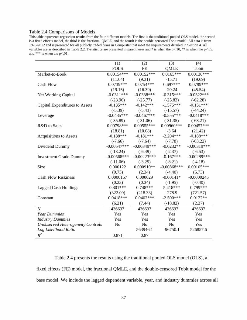
87

Table 2.4 Comparisons of Models This table represents regression results from the four different models. The first is the traditional pooled OLS model, the second

is a fixed effects model, the third is the fractional QMLE, and the fourth is the double-censored Tobit model. All data is from

1976-2012 and is presented for all publicly traded firms in Compustat that meet the requirements detailed in Section 4. All

variables are as described in Table 2.2. T-statistics are presented in parentheses and * is when the p<.10, ** is when the p<.05,

and *** is when the p<.01.

(1) (2) (3) (4)

POLS FE QMLE Tobit

Market-to-Book 0.00154*** 0.00152*** 0.0165*** 0.00136***

(11.64) (9.31) -15.71 (19.69)

Cash Flow 0.0739*** 0.0754*** 0.697*** 0.0799***

(19.15) (16.39) -20.24 (45.54)

Net Working Capital -0.0311*** -0.0338*** -0.315*** -0.0322***

(-28.96) (-25.77) (-25.83) (-62.28)

Capital Expenditures to Assets -0.135*** -0.142*** -1.575*** -0.151***

(-5.39) (-5.43) (-15.57) (-44.24)

Leverage -0.0435*** -0.0467*** -0.555*** -0.0418***

(-35.89) (-31.06) (-31.35) (-68.21)

R&D to Sales 0.00798*** 0.00555*** 0.00960*** 0.00457***

(18.81) (10.08) -3.64 (21.42)

Acquisitions to Assets -0.188*** -0.181*** -2.204*** -0.188***

(-7.66) (-7.64) (-7.78) (-63.22)

Dividend Dummy -0.00547*** -0.00349*** -0.0232** -0.00319***

(-13.24) (-6.49) (-2.37) (-6.53)

Investment Grade Dummy -0.00568*** -0.00223*** -0.167*** -0.00289***

(-11.06) (-3.29) (-8.21) (-4.18)

Size 0.000122 0.000910** -0.00868*** 0.00105***

(0.73) (2.34) (-4.40) (5.73)

Cash Flow Riskiness 0.0000157 0.000029 -0.00141* -0.0000245

(0.23) (0.34) (-1.95) (-0.40)

Lagged Cash Holdings 0.801*** 0.748*** 5.418*** 0.799***

(322.09) (218.33) -278.9 (721.57)

Constant 0.0418*** 0.0402*** -2.500*** 0.0122**

(6.21) (7.44) (-18.82) (2.27)

N 436637 436637 436637 436637

Year Dummies Yes Yes Yes Yes

Industry Dummies Yes Yes Yes Yes

Unobserved Heterogeneity Controls No No No Yes

Log Likelihood Ratio

563946.1 -96750.1 526857.6

R2 0.871 0.87

Table 2.4 presents the results using the traditional pooled OLS model (OLS), a

fixed effects (FE) model, the fractional QMLE, and the double-censored Tobit model for the

base model. We include the lagged dependent variable, year, and industry dummies across all

88

three models as well as including the time averages of the covariates, the initial value of cash

holdings, the lagged zero dummy, and lagged one dummy in the double-censored Tobit

model. Column 1 presents the results for the POLS model, column 2 presents the results for

the FE model, column 3 presents the results for the logit quasi-maximum likelihood model,

and column 4 is the double-censored Tobit model.

Overall, the coefficient estimates seem to report similar relationships between the

control variables and cash holdings. The difference across models appears to be in the size of

the coefficients. The relationships between several of the variables are as predicted by the

prior literature. Across all models, market-to-book and cash flow are positively related to

cash holdings, demonstrating that firms with better growth opportunities and more cash flow

hold larger amounts of cash. Net working capital, leverage, acquisitions to assets, dividend

dummy, and investment grade dummy are all negative and statistically significant, indicating

an inverse relationship with cash holdings. R&D to sales has a positive and statistically

significant relationship with cash holdings at a 1% level. The differences across models lie

with cash flow riskiness and capital expenditures to assets. We only find evidence of a

statistically significant relationship between cash flow riskiness and cash holdings in the

QMLE model. However, the relationship is negative and only statistically significant at the

10% level. Previous studies have found a positive relationship. Capital expenditures to assets

has a negative and statistically significant relationship with cash holdings at a 1% level. One

variable in particular, size, is not statistically significant in column 1 but becomes statistically

significant in columns 2 through 4 at varying levels. Interestingly, it is positive and

statistically significant in columns 2 and 4 which is not as predicted by prior literature. This

indicates that smaller firms hold more cash than larger ones. Finally, lagged cash holdings is

89

shown to be statistically significant at a 1% level implying that firms with higher levels of

cash holdings in the previous quarter have higher levels of cash holdings in the current

quarter. While it appears that overall the models present the same results, recall that the

inclusion of the lagged dependent variable in the POLS violates the conditional mean

assumption and the QMLE is not controlling for the unobserved heterogeneity. Thus, we

proceed with the double-censored Tobit model for subsequent regressions and discussions.

6. Results and Discussions

The following section reports the empirical results and interpretations for the entire

sample of observations, mature firms, and growth firms using all three measures of

recessions. First, the results are reported when including the macroeconomic indicators,

followed by the results when including the recession and announced recession dummy

variables.

6.1 Results with Common Macroeconomic Variables

The first regressions include common macroeconomic indicators. To measure the

economy in a way similar to the NBER, the civilian employment ratio, industrial production

index, and GDP gap are included in the regressions. In addition, other common economic

indicators are included such as the term spread and default spread.

The empirical results are shown in Table 2.5. Column 1 shows the results for all firms

while columns 2 and 3 show the results for mature and growth firms, respectively. When

looking at the macroeconomic variables located at the top of the table, employment is

90

Table 2.5 Macroeconomic Indicators and Cash Holdings This table represents the results when including macroeconomic indicators for the 1976-2012 for all data sets. Cash holdings is

the dependent variable in all regressions. Employment is the civilian employment to population ratio. Industrial Production Index

is the industrial production index provided by FRED. GDP Gap is Real GDP minus Potential Real GDP. Term Spread is the ten-

year Treasury Constant Maturity Rate minus the one-year Treasury Constant Maturity Rate. Default Spread is the difference

between Moody’s Aaa corporate bond yield and Moody’s Baa corporate bond yield. All variables are as defined in Table 2.2. T-

statistics are presented in parentheses and * is when the p<.10, ** is when the p<.05, and *** is when the p<.01.

(1) (2) (3)

All Firms Mature Firms Growth Firms

Employment -0.000561

-0.000465

-0.000997

(-0.95)

(-0.38)

(-0.70)

Industrial Production 0.00133***

0.00146***

0.00158***

(8.42)

(4.56)

(4.15)

GDP Gap -0.0000190***

-0.0000180***

-0.0000269***

(-6.27)

(-2.93)

(-3.77)

Term Spread 0.00211***

0.00205***

0.00282***

(5.68)

(2.73)

(3.15)

Default Spread 0.000303

0.00378***

-0.00208

(0.49)

(2.97)

(-1.40)

Market-to-Book 0.00140***

0.00160***

0.000368***

(20.12)

(12.10)

(2.70)

Cash Flow 0.0793***

0.0843***

0.0827***

(45.21)

(25.85)

(22.60)


-0.0308***

-0.0364***

(-63.35)

(-31.65)

(-32.09)


-0.186***

-0.119***

(-44.52)

(-25.44)

(-19.63)

Leverage -0.0419***

-0.0369***

-0.0407***

(-68.45)

(-31.20)

(-30.25)

R&D to Sales 0.00456***

0.00391***

0.00390***

(21.40)

(9.81)

(9.84)


-0.140***

-0.245***

(-63.36)

(-24.69)

(-35.49)

Dividend Dummy -0.00360***

-0.00336***

-0.00426***

(-7.34)

(-3.33)

(-3.36)

Investment Grade Dummy -0.00187***

-0.00303*

-0.00109

(-2.67)

(-1.86)

(-0.56)

Size 0.00164***

0.00186***

0.00385***

(8.73)

(4.84)

(9.51)

Cash Flow Riskiness 0.00000941

0.0000701

-0.0000997

(0.15)

(0.42)

(-0.78)


0.844***

0.835***

(721.61)

(401.74)

(388.21)

Constant 0.0187

0.0894

-0.0357

(0.41) (1.05) (-0.37)

N 436637

116068

112785

Year Dummies Yes

Yes

Yes


Yes

Yes

Log Likelihood Ratio 527060.7 136525.4 116283.3

91

negatively related to cash holdings as predicted. However, it is not statistically significant at

any conventional level in any data set. Industrial production has a positive and statistically

significant relationship with cash holdings that is significant at a 1% level. This was not as

predicted and upon further inspection, it is apparent that the industrial production index

shows the same cyclical patterns as cash holdings, falling during the start of recessions and

increasing near announcement dates.61

GDP Gap is negatively related to cash holdings and is

statistically significant at a 1% level across all three data sets. The coefficient is larger for the

growth firms and this is as expected since mature firms might not have to adjust cash

holdings practices because they potentially have access to other forms of capital. The

negative relationship is as predicted and shows that cash holdings do vary inversely with

recessions. As expected, the relationship between term spread and cash holdings is positive

and statistically significant at a 1% level. Again, the relationship is stronger for growth firms

than mature firms. The relationship between default spread and cash holdings varies across

all three data sets. In the entire data set, the relationship is positive but not statistically

different from zero. For mature firms, the relationship is positive and statistically significant

at a 1% level. Growth firms do not show a statistically significant relationship between the

default spread and cash holdings. While it is hypothesized that the default spread should

have a negative relationship with cash holdings based on prior literature, Figure 2.2 did not

show a negative relationship. A positive relationship was not predicted, but we do not place

too much weight on the results with this variable since the other variables show the predicted

variation of cash holdings during business cycles.

61

The plot of these two variables and the announced recession dates can be found in appendix Figure A.3.2.

92

The control variables show similar relationships with cash holdings as discussed in

Table 2.4. In addition, they remain consistent with the previous literature with the exception

of size which remains positive and statistically significant at a 1% level.

Overall, it appears that the common economic indicators are related to corporate cash

holdings. The majority of the variables are statistically significant in the regressions and are

of the appropriate sign as predicted by the graphs of the series. This demonstrates that cash

holdings do vary with business conditions; they are lower during expansions and higher

during recessions. However, Figure 2.1 shows potentially different relationships between

recessions and announced recession dates. Thus, we proceed by examining recession periods

using dummy variables.

6.2 Results with Recession Indicators

The main focus of this paper is whether business cycles affect the cash holdings of

firms. We have shown that common economic indicators are correlated with corporate cash

holdings, thus showing a variation in cash across the business cycle. Here, recession

indicators are included to show how cash holdings react during recessions.

The results for the entire sample of public firms are located in the first two columns

of Table 2.6. Column 1 includes the recession dummy and the second column includes both

the recession dummy and the macroeconomic indicators. The coefficient on recession dummy

in the first column is negative but not statistically different from zero. Recession dummy in

column 2 is again negative, but is statistically significant at a 5% level. The indicator is

included with the five macroeconomic variables to show that these variables do not capture

the entire change in cash holdings. It is interesting that when including the macroeconomic

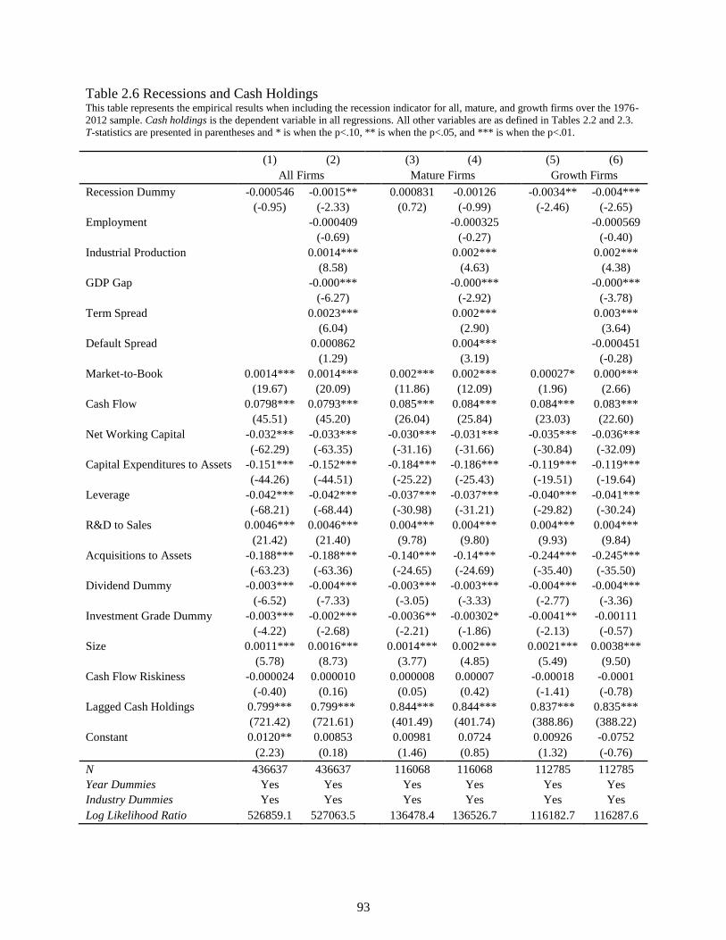
93

Table 2.6 Recessions and Cash Holdings This table represents the empirical results when including the recession indicator for all, mature, and growth firms over the 1976-

2012 sample. Cash holdings is the dependent variable in all regressions. All other variables are as defined in Tables 2.2 and 2.3.

T-statistics are presented in parentheses and * is when the p<.10, ** is when the p<.05, and *** is when the p<.01.

(1) (2) (3) (4) (5) (6)


Recession Dummy -0.000546 -0.0015**

0.000831 -0.00126

-0.0034** -0.004***

(-0.95) (-2.33)

(0.72) (-0.99)

(-2.46) (-2.65)

Employment

-0.000409

-0.000325

-0.000569

(-0.69)

(-0.27)

(-0.40)

Industrial Production

0.0014***

0.002***

0.002***

(8.58)

(4.63)

(4.38)

GDP Gap

-0.000***

-0.000***

-0.000***

(-6.27)

(-2.92)

(-3.78)

Term Spread

0.0023***

0.002***

0.003***

(6.04)

(2.90)

(3.64)

Default Spread

0.000862

0.004***

-0.000451

(1.29)

(3.19)

(-0.28)

Market-to-Book 0.0014*** 0.0014***

0.002*** 0.002***

0.00027* 0.000***

(19.67) (20.09)

(11.86) (12.09)

(1.96) (2.66)

Cash Flow 0.0798*** 0.0793***

0.085*** 0.084***

0.084*** 0.083***

(45.51) (45.20)

(26.04) (25.84)

(23.03) (22.60)

Net Working Capital -0.032*** -0.033***

-0.030*** -0.031***

-0.035*** -0.036***

(-62.29) (-63.35)

(-31.16) (-31.66)

(-30.84) (-32.09)

Capital Expenditures to Assets -0.151*** -0.152***

-0.184*** -0.186***

-0.119*** -0.119***

(-44.26) (-44.51)

(-25.22) (-25.43)

(-19.51) (-19.64)

Leverage -0.042*** -0.042***

-0.037*** -0.037***

-0.040*** -0.041***

(-68.21) (-68.44)

(-30.98) (-31.21)

(-29.82) (-30.24)

R&D to Sales 0.0046*** 0.0046***

0.004*** 0.004***

0.004*** 0.004***

(21.42) (21.40)

(9.78) (9.80)

(9.93) (9.84)

Acquisitions to Assets -0.188*** -0.188***

-0.140*** -0.14***

-0.244*** -0.245***

(-63.23) (-63.36)

(-24.65) (-24.69)

(-35.40) (-35.50)

Dividend Dummy -0.003*** -0.004***

-0.003*** -0.003***

-0.004*** -0.004***

(-6.52) (-7.33)

(-3.05) (-3.33)

(-2.77) (-3.36)

Investment Grade Dummy -0.003*** -0.002***

-0.0036** -0.00302*

-0.0041** -0.00111

(-4.22) (-2.68)

(-2.21) (-1.86)

(-2.13) (-0.57)

Size 0.0011*** 0.0016***

0.0014*** 0.002***

0.0021*** 0.0038***

(5.78) (8.73)

(3.77) (4.85)

(5.49) (9.50)

Cash Flow Riskiness -0.000024 0.000010

0.000008 0.00007

-0.00018 -0.0001

(-0.40) (0.16)

(0.05) (0.42)

(-1.41) (-0.78)

Lagged Cash Holdings 0.799*** 0.799***

0.844*** 0.844***

0.837*** 0.835***

(721.42) (721.61)

(401.49) (401.74)

(388.86) (388.22)

Constant 0.0120** 0.00853

0.00981 0.0724

0.00926 -0.0752

(2.23) (0.18) (1.46) (0.85) (1.32) (-0.76)

N 436637 436637

116068 116068

112785 112785

Year Dummies Yes Yes

Yes Yes

Yes Yes


Yes Yes

Yes Yes

Log Likelihood Ratio 526859.1 527063.5 136478.4 136526.7 116182.7 116287.6

94

variables, the magnitude of the recession dummy remains large and increases. This reinforces

what is shown in Panel A of Figure 2.1: cash holdings decline during the initial stages of

recessions. Looking at the firm characteristics, the results are similar to prior tables and thus

for brevity, the results will not be discussed. The results lead to the conclusion that cash

holdings decline during recession even when controlling for other macroeconomic indicators.

The macroeconomic indicators are of the predicted sign and are all statistically

significant. Employment and GDP Gap both have a negative relationship with cash holdings

however, only GDP Gap is statistically significant at a 1% level. Industrial production and

term spread have a positive and statistically significant relationship with cash holdings at a

1% level. Default spread has a positive relationship with cash holdings but is not statistically

different from zero. Thus, the results from columns 1 and 2 yield the result that cash holdings

do decline during recessions. In addition, the macroeconomic variables are not capturing the

complete decline in cash holdings, suggesting that corporate cash holdings are not declining

proportionally to the economy.

The results for mature firms are located in columns 3 and 4. Again, the results are

first presented with the recession dummy followed by both the recession dummy and

macroeconomic variables. Recession dummy is positive but not statistically different from

zero in column 3. When including the macroeconomic indicators along with the recession

dummy, recession dummy is negative, but not statistically different from zero in column 4.

The estimated coefficients on the macroeconomic variables are similar to the results in

previous tables, with the exception that the default spread is positive and statistically

significant at a 1% level. Thus, the cash holdings of mature firms do not appear to decrease

during recessions, which suggests that while the cash holdings of mature firms do vary across

95

the business cycle, they do not show the large decline during recessions as represented in

Figure 2.1. This is potentially because mature firms have access to other forms of capital and

do not have to draw down cash holdings.

The results for growth firms are presented in columns 5 and 6 of Table 2.6. The

relationship between cash holdings and recession dummy is negative and statistically

significant at a 1% level in column 5. The relationship between recession dummy and cash

holdings remains negative and statistically significant at a 1% level after adding in the

macroeconomic variables. The decline in cash holdings shown in Figure 2.1 is seen amongst

growth firms during recessions. This decline could be the result of reduced access to capital.

As predicted, growth firms show an exaggerated change in cash holdings during recessions

than mature firms.

While it is assumed that cash holdings increase during recessions, as shown by the

macroeconomic indicators, it is found that these variables are not capturing the initial decline

in cash holdings at the start of recessions that is primarily found in growth firms.

6.3 Estimation with Announced Recession Indicator

Thus far, we have shown that common economic indicators are correlated with

corporate cash holdings and that these indicators fail to capture all of the variation in cash

holdings during recessions. Attention is now focused on the announcement period of

recessions. Because recessions are announced after they have begun, there is a lag between

when the economy enters a recession and when the public knows the economy is in a

recession. Panel B of Figure 2.1 shows that cash holdings increase during the announcement

96

Table 2.7 Announced Recessions and Cash Holdings This table represents the empirical results when including the announced recession indicator for all, mature, and growth firms

over the 1976-2012 sample. Cash holdings is the dependent variable in all regressions. All other variables are as defined in

Tables 2.2 and 2.3. T-statistics are presented in parentheses and * is when the p<.10, ** is when the p<.05, and *** is when the

p<.01.

(1) (2) (3) (4) (5) (6)


Announced Recession Dummy 0.002*** 0.0012**

0.003*** 0.00142

0.004*** 0.0026*

(3.93) (1.96)

(2.61) (1.13)

(3.00) (1.78)

Employment

-0.0005

-0.0003

-0.0008

(-0.86)

(-0.26)

(-0.59)


0.0013***

0.0014***

0.0016***

(8.37)

(4.48)

(4.07)

GDP Gap

-0.000***

-0.0000**

-0.000***

(-5.61)

(-2.51)

(-3.24)

Term Spread

0.0021***

0.0020***

0.0028***

(5.63)

(2.70)

(3.11)

Default Spread

0.000226

0.0037***

-0.00229

(0.36)

(2.87)

(-1.54)

Market-to-Book 0.001*** 0.0014***

0.002*** 0.0016***

0.0003** 0.0004***

(19.73) (20.12)

(11.86) (12.11)

(2.04) (2.67)

Cash Flow 0.080*** 0.0793***

0.085*** 0.0842***

0.084*** 0.0827***

(45.54) (45.20)

(26.01) (25.84)

(23.06) (22.59)


-0.030*** -0.031***

-0.035*** -0.036***

(-62.25) (-63.34)

(-31.17) (-31.64)

(-30.81) (-32.08)


-0.184*** -0.186***

-0.118*** -0.119***

(-44.19) (-44.52)

(-25.22) (-25.44)

(-19.48) (-19.61)

Leverage -0.042*** -0.042***

-0.037*** -0.037***

-0.040*** -0.041***

(-68.21) (-68.45)

(-31.01) (-31.21)

(-29.82) (-30.24)

R&D to Sales 0.005*** 0.0046***

0.004*** 0.0039***

0.004*** 0.0039***

(21.41) (21.40)

(9.78) (9.82)

(9.92) (9.83)


-0.14*** -0.140***

-0.244*** -0.245***

(-63.20) (-63.36)

(-24.65) (-24.69)

(-35.38) (-35.48)

Dividend Dummy -0.003*** -0.004***

-0.003*** -0.003***

-0.004*** -0.004***

(-6.53) (-7.33)

(-3.04) (-3.33)

(-2.77) (-3.37)


-0.004** -0.0031*

-0.004** -0.0011

(-4.17) (-2.69)

(-2.25) (-1.88)

(-2.13) (-0.55)

Size 0.001*** 0.0016***

0.002*** 0.002***

0.002*** 0.004***

(5.76) (8.72)

(3.84) (4.82)

(5.50) (9.50)


0.00001 0.0001

-0.0002 -0.0001

(-0.40) (0.15)

(0.08) (0.43)

(-1.39) (-0.77)


0.845*** 0.844***

0.837*** 0.835***

(721.45) (721.60)

(401.56) (401.76)

(388.94) (388.24)

Constant 0.0122** 0.0258

0.0094 0.0871

0.0094 -0.0474

(2.27) (0.55) (1.40) (1.02) (1.34) (-0.48)

N 436637 436637

116068 116068

112785 112785


Yes Yes

Yes Yes


Yes Yes

Yes Yes

Log Likelihood Ratio 526865.3 527063.4 136484.7 136528.1 116184.1 116285

97

periods after initially declining during the beginning of the recession periods. We include a

dummy variable for recession announcement dates to capture this relationship.

The results when including an announced recession dummy are included in Table 2.7.

The results for all firms are located in the first two columns. The first column includes the

announced recession indicator and the second column adds five macroeconomic variables

along with the announced recession dummy. Similar to the recession dummy, the indicator is

included with the five macroeconomic variables to show that these variables do not capture

the full change in cash holdings.

The relationship between cash holdings and announced recession dummy is positive

and statistically significant at a 1% level in the first column. After controlling for the

common determinants of corporate cash holdings, an increase among cash holdings during

announced recessions is found. Similar to the results in Table 2.6, most of the relationships

between the firm characteristics and cash holdings are as predicted. When including the

macroeconomic variables, the relationship between announced recession dummy and cash

holdings remains positive and statistically significant at a 5% level. Thus, it is found that

cash holdings increase during announced recession periods. Coupling these results with those

from Table 2.6, it is clear that while there is an initial decrease in cash holdings during the

periods of a recession, cash holdings eventually increase. Furthermore, this increase occurs

during the time that the NBER has announced that the economy is in a recession.

The results for mature firms can be found in columns 3 and 4. As with the entire data

set, the relationship with announced recession dummy is positive and statistically significant

at a 1% level in column 3. However, when including the macroeconomic indicators, the

relationship remains positive but is no long statistically different from zero. This suggests

98

that while mature firms do alter cash holding during the announcement periods of the

recessions, the macroeconomic variables are capturing all of the increase. The expected

relationship between cash holdings and recessions that prior papers have shown using

macroeconomic indicators could be driven by mature firms and an increase in cash.

Lastly, the results for the growth firms are presented in columns 5 and 6. When

controlling for firm characteristics, the relationship between the announced recession dummy

and cash holdings is positive and statistically significant at a 1% level. As predicted, the

coefficient on the announced recession dummy is larger than that for mature firms,

demonstrating that mature firms do respond by holdings less cash than growth firms.

However, both types of firms increase holdings of cash due to a potential decline in the

availability of credit. When including the macroeconomic variables, the relationship between

cash holdings and announced recession dummy remains positive and marginally significant

at a 10% level. Unlike with the mature firms, the macroeconomic variables are not capturing

the entire increase in cash holdings experienced by growth firms.

6.4 First Quarter Announced Recession

In order to examine whether the increase in cash holdings represents an

announcement effect, a dummy variable for the first quarter of an announced recession is

included. If the results show that cash holdings jump during this quarter, this is more

evidence of the announcement effect. The results are presented in Table 2.8. As in previous

tables, the odd columns include the announced recession indicator and the even columns add

in the five macroeconomic variables.

99

Table 2.8 First Quarter of an Announced Recession and Cash Holdings This table represents the empirical results when including the recession indicator for all, mature, and growth firms over the 1976-



(1) (2) (3) (4) (5) (6)


First Quarter Announced Recession 0.004*** 0.004***

0.005*** 0.004***

0.005*** 0.0046**

(6.15) (5.23)

(3.75) (2.76)

(3.02) (2.57)

Employment

-0.0007

-0.0006

-0.0010

(-1.11)

(-0.52)

(-0.73)


0.001***

0.002***

0.002***

(8.59)

(4.69)

(4.19)

GDP Gap

-0.00***

-0.000**

-0.000***

(-5.60)

(-2.54)

(-3.45)

Term Spread

0.002***

0.0019**

0.003***

(5.26)

(2.45)

(2.95)

Default Spread

-0.0002

0.0032**

-0.0026*

(-0.33)

(2.44)

(-1.70)

Market-to-Book 0.001*** 0.001***

0.002*** 0.002***

0.0003** 0.000***

(19.76) (20.12)

(11.88) (12.10)

(2.06) (2.69)

Cash Flow 0.08*** 0.079***

0.085*** 0.084***

0.084*** 0.083***

(45.58) (45.23)

(26.05) (25.86)

(23.08) (22.61)


-0.03*** -0.03***

-0.04*** -0.04***

(-62.27) (-63.34)

(-31.13) (-31.62)

(-30.84) (-32.10)


-0.18*** -0.19***

-0.12*** -0.12***

(-44.24) (-44.54)

(-25.22) (-25.44)

(-19.49) (-19.62)

Leverage -0.04*** -0.04***

-0.04*** -0.04***

-0.04*** -0.04***

(-68.22) (-68.44)

(-30.98) (-31.20)

(-29.84) (-30.25)

R&D to Sales 0.005*** 0.005***

0.004*** 0.004***

0.004*** 0.004***

(21.42) (21.40)

(9.79) (9.81)

(9.92) (9.83)


-0.14*** -0.14***

-0.24*** -0.25***

(-63.22) (-63.37)

(-24.65) (-24.69)

(-35.39) (-35.49)

Dividend Dummy -0.00*** -0.00***

-0.00*** -0.00***

-0.00*** -0.00***

(-6.55) (-7.36)

(-3.03) (-3.33)

(-2.80) (-3.39)


-0.004** -0.003*

-0.004** -0.0011

(-4.17) (-2.66)

(-2.22) (-1.85)

(-2.12) (-0.54)

Size 0.001*** 0.002***

0.00*** 0.00***

0.00*** 0.004***

(5.77) (8.72)

(3.80) (4.81)

(5.50) (9.51)


0.0000 0.0001

-0.0002 -0.0001

(-0.40) (0.15)

(0.06) (0.42)

(-1.39) (-0.78)


0.84*** 0.84***

0.84*** 0.835***

(721.54) (721.62)

(401.53) (401.75)

(388.93) (388.25)

Constant 0.0122** 0.0326

0.0097 0.102

0.0095 -0.0468

(2.26) (0.69) (1.45) (1.20) (1.35) (-0.48)

N 436637 436637

116068 116068

112785 112785


Yes Yes

Yes Yes


Yes Yes

Yes Yes


100

The relationship between cash holdings and first quarter announced recession is

positive and statistically significant at a 1% level across all three data sets, regardless of

whether macroeconomic controls are included. This demonstrates that an increase in cash

holdings is found during the quarter that the NBER announced a recession. The increase is

found on top of the macroeconomic indicators suggesting that the increase in the first quarter

is not being captured by these variables. Since these results are found across all three data

sets, it suggests that the cash holdings of all firms increase once they have confirmation that

the economy is in a recession. When including macroeconomic indicators, the magnitude of

the coefficient is larger for growth firms than for mature firms, suggesting that growth firms

have to build up larger reserves to prepare for tighter credit conditions.

In appendix Table A.2.2 and as a robustness test, we include the first full quarter after

a recession announcement is made by the NBER. A positive and significant relationship is

not found across any of the data sets. Interestingly, a statistically significant negative

relationship is found in some of the regressions. Looking at Figure 2.1, cash holdings does

not grow as quickly in subsequent quarters of an announced recession and sometimes appears

to slightly decrease. Thus, it is evident that the increase in cash holdings occurs during the

first quarter that companies have confirmation that the economy is in a recession. We find

that these results support an announcement effect in cash holdings and not the precautionary

cash holdings theory.

As a final robustness check, the results off which are shown in appendix Table A.2.3,

we measure the announced recession period using Whole Quarter Announced Recession,

which only includes quarters when they are completely defined as an announced recession

period. The relationship between cash holdings and this dummy variable is only statistically

101

significant for all firms when the macroeconomic variables are included. The results are

found in column 2 and the relationship is negative and statistically significant. Again, this

result documents that the increase takes place during the quarter of an announcement.

Thus, it appears that there is an announcement effect among companies. Cash

holdings decline during the initial unannounced periods of recessions but once the recession

is announced, companies increase cash holdings. The precautionary motive states that firms

hold cash as a safeguard against recessionary periods. The motive does not state that firms

hoard cash once the recession is announced. We do not find evidence of the precautionary

motive among firms and instead find evidence of an announcement effect.

7. Constrained and Unconstrained Firms

In this section, we present evidence of the change in cash holdings during recession

and announced recession periods for constrained and unconstrained firms. Several papers

have analyzed the variation of cash holdings for these firms over the business cycle but none

of these have discovered the announcement effect documented above. Following Almeida, et

al. (2004), financially constrained and unconstrained firms are defined three different ways.62

The first is based on firm size. Firms are sorted into deciles based on total assets for each

quarter and the top (bottom) three deciles are defined as unconstrained (constrained) firms.

The argument is that smaller firms are typically younger and less well known. The second

and third measures are bond and commercial paper ratings. These are measured similarly,

with the exception that the bond rating data is the S&P long-term rating and the commercial

rating data is the S&P short-term rating. If a firm has never had a rating and holds a positive

62

Almeida, et al. (2009) also use the KZ Index to classify constrained and unconstrained firms, however they find

that this measure is negatively correlated with the other measures so it is excluded from our analysis.

102

value for debt, then the firm is classified as constrained. Unconstrained firms are classified as

firms that have been rated during the sample.63

The argument here is that firms without

ratings do not have the ease of access to external financing. It is expected that firms that are

constrained will have a larger jump in cash holdings at the announcement of a recession to

guard against potential difficulty in obtaining capital.

7.1 Results for Constrained and Unconstrained Firms

Results for the constrained and unconstrained firms can be found in Table 2.9. The

results are presented based on bond rating however, the other two classifications of

constrained and unconstrained firms yield similar results.64

For brevity, only the

macroeconomic variables, recession dummy, announced recession dummy, and first quarter

announced recession are reported. Results for unconstrained and constrained firms can be

found in Panels A and B, respectively.

For unconstrained firms, the expected variation is found between cash holdings and

the macroeconomic indicators. The relationship between cash holdings and both employment

and GDP gap is negative. Like previous regressions, only the GDP gap is statistically

significant at a 1% level. The relationship between industrial production and cash holdings

is positive and statistically significant at a 1% level. Term spread and default spread vary in

significance across the three columns. Looking at recession dummy located in the first two

columns, a negative relationship is seen with cash holdings. The relationship is statistically

significant at a 10% level once the macroeconomic variables are included. This suggests that

a slight decline in cash holdings is found during recessions that is not being captured by the

63

In addition, Almeida, et al. (2004) classify firms with no rating and no debt as unconstrained. 64


103

Table 2.9 Business Cycles and Cash Holdings for Constrained and Unconstrained Firms This table represents the empirical results for constrained and unconstrained firms based on bond rating over the 1976-2012 sample. Firms are classified as unconstrained if they

have a bond rating some time during the sample. Firms are classified as constrained if they never have a bond rating and report positive value for debt. Cash holdings is the

dependent variable in all regressions. All other control variables are included in the regressions but are omitted for brevity. All variables are as defined in Table 2.3. T-statistics are

presented in parentheses and * is when the p<.10, ** is when the p<.05, and *** is when the p<.01.

Panel A: Unconstrained Firms by Bond Rating (1) (2) (3) (4) (5) (6)

Unconstrained by Bond Rating

Recession Dummy Announced Recession Dummy First Quarter Announced Recession

Recession Dummy -0.000683 -0.00141*

(-0.92) (-1.70)

Announced Recession Dummy

0.00306*** 0.00241***

(4.43) (3.12)

First Quarter Announced Recession

0.00456*** 0.00423***

(5.18) (4.40)

Employment

-0.000416

-0.000529

-0.000586

(-0.54)

(-0.69)

(-0.77)


0.000937***

0.000893***

0.000919***

(4.64)

(4.44)

(4.57)

GDP Gap

-0.0000159***

-0.0000130***

-0.0000139***

(-4.17)

(-3.28)

(-3.61)

Term Spread

0.000845*

0.000585

0.000472

(1.70)

(1.21)

(0.97)

Default Spread

0.000992

0.000276

-0.000179

(1.17) (0.35) (-0.22)

N 190689 190689 190689 190689 190689 190689

Year Dummies Yes Yes Yes Yes Yes Yes

Industry Dummies Yes Yes Yes Yes Yes Yes


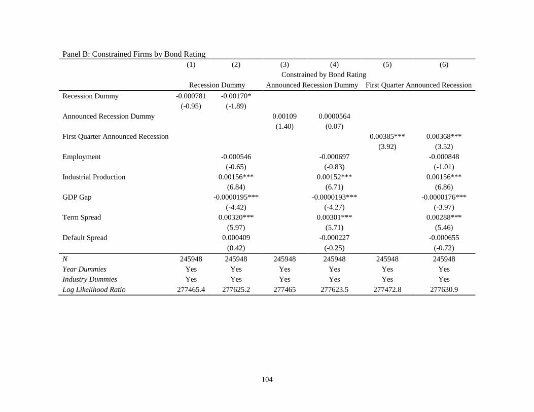
104

Panel B: Constrained Firms by Bond Rating (1) (2) (3) (4) (5) (6)

Constrained by Bond Rating

Recession Dummy Announced Recession Dummy First Quarter Announced Recession

Recession Dummy -0.000781 -0.00170*

(-0.95) (-1.89)

Announced Recession Dummy

0.00109 0.0000564

(1.40) (0.07)

First Quarter Announced Recession

0.00385*** 0.00368***

(3.92) (3.52)

Employment

-0.000546

-0.000697

-0.000848

(-0.65)

(-0.83)

(-1.01)


0.00156***

0.00152***

0.00156***

(6.84)

(6.71)

(6.86)

GDP Gap

-0.0000195***

-0.0000193***

-0.0000176***

(-4.42)

(-4.27)

(-3.97)

Term Spread

0.00320***

0.00301***

0.00288***

(5.97)

(5.71)

(5.46)

Default Spread

0.000409

-0.000227

-0.000655

(0.42) (-0.25) (-0.72)

N 245948 245948 245948 245948 245948 245948

Year Dummies Yes Yes Yes Yes Yes Yes

Industry Dummies Yes Yes Yes Yes Yes Yes

Log Likelihood Ratio 277465.4 277625.2 277465 277623.5 277472.8 277630.9

105

macroeconomic variables. There is a positive and statistically significant relationship at a 1%

level found between cash holdings and announced recession dummy in columns 3 and 4.

Even though these firms have less financial constraints than other firms, they still increase

holdings of cash once a recession is announced. Finally, looking at the results for the first

quarter of an announced recession, a positive relationship is seen between cash holdings and

first quarter announced recession suggesting that firms increase cash holdings during the

quarter in which a recession is announced. Thus, we find evidence of an announcement effect

for unconstrained firms.

The results for constrained firms are found in Panel B. While we observe variation

across business cycles, the results with the recession dummies differ greatly from the

unconstrained firms. While a slight decline in cash holdings is found at the start of

recessions, the relationship between the announced recession dummy and cash holdings is

positive but not statistically different from zero. Thus, it is not shown that constrained firms

increase cash holdings over the entire announced recession period as documented for

unconstrained firms. This is not unexpected since these firms would have a harder time

accessing forms of capital in order to accumulate cash. Looking at the results in columns 5

and 6, the relationship between first quarter announced recession and cash holdings is

positive and statistically significant at a 1% level. This is surprising that constrained firms

increase cash holdings the quarter a recession is announced however, the magnitude of the

increase is smaller than for the unconstrained firms.

In summary, it is shown that unconstrained and constrained firms are subject to an

announcement effect that has been undocumented prior to this paper. Both groups of firms

increase cash holdings the quarter a recession is announced. However, constrained firms do

106

not increase cash holdings over the entire period of the announced recession as with

unconstrained firms. This suggests that firms may be able to use access to the bond market or

commercial paper market to increase holdings of cash during recessions.

8. Conclusion

This paper adds to the corporate cash holdings literature by documenting a

relationship between cash holdings and business cycles. The random effects double censored

Tobit model is used, which is unique to the cash holdings literature and ideally suited for the

standard measure of corporate cash holdings because it requires that the dependent variable

be a fractional value between and including zero and one. In addition, several different data

sets are employed: one that contains all firms with non-missing observations in Compustat, a

mature firm data set, and a growth firm data set.

The main result of this paper is that cash holdings display cyclical patterns. Cash

holdings appear to fall during the initial periods of recessions and rise during the latter half.

Unlike previous research on the relationship between cash holdings and recessions, we

additionally control for reported business cycles and announced periods of business cycles

from the NBER. The rise in cash holdings documented during business cycles appears to

coincide with recession announcements made by the NBER. In finding that companies react

to the announcement of a recession, we do not find evidence of the precautionary motive for

cash holdings and instead find an announcement effect for corporate cash holdings during

recessions. We also find that both the decline in cash holdings during the initial periods of

recessions and the announcement effect is greater for growth firms than mature firms.

107

The relationship is also examined for unconstrained and constrained firms. While

these firms are classified in three different ways, the results remain similar: both groups of

firms show evidence of an announcement effect by increasing cash holdings the quarter a

recessions is announced. This previously undocumented effect is greater for unconstrained

firms than constrained firms.

In conclusion, this paper adds to the literature by documenting an announcement

effect in cash holdings for a wide range of firms. While it is assumed that cash holdings are

larger during recessions, we present evidence that the increase during recessions is the result

of a confirmation of a recession due to an official announcement by the NBER.

108

References

Almeida, H., M. Campello, and M. S. Weisbach, 2004, The cash flow sensitivity of cash,

Journal of Finance, 59, 1777-1804.

Bates, T. W., K. M. Kahle, and R. M. Stulz, 2009, Why do US firms hold so much more cash

than they used to?, Journal of Finance 64, 1985-2021.

Baum, C. F., M. Caglayan, N. Ozkan, and O. Talavera, 2006, The impact of macroeconomic

uncertainty on non-financial firms’ demand for liquidity, Review of Financial Economics

15, 289-304.

Brown, J. R., and B. C. Petersen, 2011, Cash holdings and R&D smoothing, Journal of

Corporate Finance 17, 694-709.

Campello, M., J. R. Graham, and C. R. Harvey, 2010, The real effects of financial constraints:

Evidence from a financial crisis, Journal of Financial Economics 97, 470-487.

Chamberlain, G., 1980, Analysis of variance with qualitative data, Review of Econometric

Studies 47, 225-238.

Chen, N.-F., 1991, Financial investment opportunities and the macroeconomy, Journal of

Finance 46, 1467-1484.

Colquitt, L. L., D. W. Sommer, and N. H. Godwin, 1999, Determinants of cash holdings by

property-liability insurers, Journal of Risk and Insurance 66, 401-415.

Duchin, R., O. Ozbas, and B. A. Sensoy, 2010, Costly external finance, corporate investment,

and the subprime mortgage credit crisis, Journal of Financial Economics 97, 418-435.

Fama, E. and K. French, 1989, Business conditions and expected returns on stocks and bonds,

Journal of Financial Economics 25, 23-49.

Ferreira, Miguel A., Custodio, Claudia and Raposo, Clara C., Cash Holdings and Business

Conditions (February 2005). Available at SSRN: http://ssrn.com/abstract=608664

Fresard, L., 2010, Financial strength and product market behavior: The real effects of corporate

cash holdings, Journal of Finance 65, 1097-1122.

109

Goldstein, J., 2011, Companies Have Been Holding More Cash For Decades, NPR Planet Money

Blog, 20 September 2011, <

http://www.npr.org/blogs/money/2011/09/19/140605375/companies-have-

been-piling-up-cash-for-decades>.

Han, S. J., and H. P. Qiu, 2007, Corporate precautionary cash holdings, Journal of Corporate

Finance 13, 43-57.

Harford, J., 1999, Corporate cash reserves and acquisitions, Journal of Finance 54, 1969-1997.

Ivanshina, V. and D. Scharfstein, 2010, Bank lending during the financial crisis of 2008, Journal

of Financial Economics 97, 319-338.

Kahle, K. M., and R. M. Stulz, 2013, Access to capital, investment and the financial crisis,


Keynes, J. M., 1936. The General Theory of Employment, Interest and Money. Harcourt Brace,

London.

Lins, K. V., H. Servaes, and P. Tufano, 2010, What drives corporate liquidity? An international

survey of cash holdings and lines of credit, Journal of Financial Economics 98, 160-176.

Loudermilk, M., 2007, Estimation of Fractional Dependent Variables in Dynamic Panel Data

Models With an Application to firm Dividend Policy, Journal of Business & Economic

Statistics 25, 462-472.

Mikkelson, W. H., and M. M. Partch, 2003, Do persistent large cash reserves hinder

performance?, Journal of Financial and Quantitative Analysis 38, 275-294.

Mundlak, Y., 1978, On the pooling of time series and cross section data, Econometrica 46, 69-

85.

Opler, T., L. Pinkowitz, R. Stulz, and R. Williamson, 1999, The determinants and implications of

corporate cash holdings, Journal of Financial Economics 52, 3-46.

Papke, L. E., and J. M. Wooldridge, 1996, Econometric methods for fractional response variable

with an application to 401(k) plan participation rates, Journal of Applied Econometrics

11, 619-632.

Papke, L. E., and J. M. Wooldridge, 2008, Panel data methods for fractional response variables

with an application to test pass rates, Journal of Econometrics 145, 121-133.

Pinkowitz, L., R. Stulz, and R. Williamson, 2013, Is there a high cash holdings puzzle after the

financial crisis?, working paper.

National Bureau of Economic Research (NBER), 2010, US Business Cycle Expansions and

Contractions, August 17, 2011 <http://www.nber.org/cycles.html>.

110

Von Eije, J. H., What Causes Differences in Cash Holdings between Listed and Unlisted Firms

Around the World? (February 23, 2012). Available at SSRN:

http://ssrn.com/abstract=2010053 or http://dx.doi.org/10.2139/ssrn.2010053

Wheelock, D. C. and M. E. Wohar, Can the term spread predict output growth and recessions? A

survey of the literature, Federal Reserve Bank of St. Louis Review 91, 419-440.

111

Appendix

Table A.2.1 Variable Descriptions This table provides the corporate variable names and definitions used in the paper.

Variable Definition Expected

Relationship

Cash Holdings Cash, Cash Equivalents, and Marketable Securities divided by

Total Assets

Market-to-Book Market Value per Share to the stated Book Value of Equity +

Cash Flow Earnings after Interest, Taxes, and Dividends, but before

Depreciation, divided by Total Assets +

Net Working Capital Net Working Capital minus Cash, Cash Equivalents, and

Marketable Securities divided by Total Assets -

Capital Expenditure to Assets Earnings after Interest, Taxes, and Dividends, but before

Depreciation, divided by Total Assets -

Leverage Long Term Debt plus Current Debt divided by Total Assets + / -

R&D to Sales Research and Development divided by Sales. If R&D is missing

in Compustat then it is set to zero. +

Acquisitions-to-Assets Acquisitions divided by Total Assets -

Dividend Dummy Indicator variable equal to one if the company pays a common

dividend and zero otherwise -

Investment Grade Dummy

Indicator variable equal to one if a company has a long-term bond

rating of BBB- and above or a short-term commercial paper rating

of A-3 and above, otherwise the dummy equals zero

-

Size Natural log of a firm’s Total Assets in 2009 dollars, using the

consumer price index to account for inflation -

Cash Flow Riskiness

The standard deviation of industry cash flows calculated as

suggested by Opler, et al. (1999). It requires the standard

deviation of cash flows for the previous twenty observations (five

years), if available. We do require that firms have at least one year

of data to calculate cash flow riskiness. Observations are then

averaged across the two-digit SIC code.

+

112

Table A.2.2 First Whole Quarter of an Announced Recession Results This table represents the empirical results when including the recession indicator for all, mature, and growth firms over the 1976-



(1) (2) (3) (4) (5) (6)


First Whole Quarter Announced Recess -0.00*** -0.002**

-0.001 -0.0004

-0.01*** -0.0026

(-4.29) (-2.20)

(-0.81) (-0.26)

(-2.96) (-1.42)

Employment

-0.0003

-0.0004

-0.0006

(-0.57)

(-0.36)

(-0.40)


0.001***

0.002***

0.002***

(7.88)

(4.47)

(3.78)

GDP Gap

-0.00***

-0.00***

-0.00***

(-5.82)

(-2.87)

(-3.48)

Term Spread

0.002***

0.002***

0.003***

(5.75)

(2.72)

(3.21)

Default Spread

0.0005

0.00***

-0.0016

(0.87)

(2.92)

(-1.08)

Market-to-Book 0.00*** 0.00***

0.00*** 0.00***

0.000** 0.00***

(19.69) (20.12)

(11.85) (12.10)

(2.02) (2.70)

Cash Flow 0.08*** 0.08***

0.09*** 0.08***

0.08*** 0.08***

(45.53) (45.20)

(26.03) (25.85)

(23.04) (22.60)


-0.03*** -0.03***

-0.04*** -0.04***

(-62.25) (-63.34)

(-31.16) (-31.64)

(-30.82) (-32.09)


-0.18*** -0.19***

-0.12*** -0.12***

(-44.23) (-44.52)

(-25.23) (-25.44)

(-19.50) (-19.62)

Leverage -0.04*** -0.04***

-0.04*** -0.04***

-0.04*** -0.04***

(-68.19) (-68.44)

(-30.99) (-31.21)

(-29.83) (-30.25)

R&D to Sales 0.00*** 0.00***

0.00*** 0.00***

0.00*** 0.00***

(21.42) (21.40)

(9.78) (9.81)

(9.92) (9.83)


-0.14*** -0.14***

-0.24*** -0.25***

(-63.22) (-63.36)

(-24.66) (-24.69)

(-35.39) (-35.48)


-0.00*** -0.00***

-0.00*** -0.00***

(-6.52) (-7.33)

(-3.03) (-3.33)

(-2.77) (-3.37)


-0.004** -0.003*

-0.004** -0.001

(-4.18) (-2.68)

(-2.24) (-1.87)

(-2.13) (-0.56)

Size 0.00*** 0.00***

0.00*** 0.00***

0.00*** 0.00***

(5.73) (8.73)

(3.79) (4.83)

(5.49) (9.51)


0.00001 0.00007

-0.0002 -0.0001

(-0.42) (0.15)

(0.06) (0.43)

(-1.42) (-0.78)


0.85*** 0.84***

0.84*** 0.84***

(721.54) (721.60)

(401.49) (401.74)

(388.87) (388.23)

Constant 0.012** 0.0129

0.00966 0.092

0.00938 -0.0631

(2.28) (0.27) (1.44) (1.08) (1.33) (-0.64)

N 436637 436637

116068 116068

112785 112785


Yes Yes

Yes Yes


Yes Yes

Yes Yes

Log Likelihood Ratio 526867 527063 136479 136526 116186 116286

113

Table A.2.3 Recession Indicator Using Whole Quarters and Cash Holdings This table represents the empirical results when including the recession indicator for all, mature, and growth firms over the 1976-



(1) (2) (3) (4) (5) (6)


Whole Quarter Announced Recession -0.0010 -0.00***

-0.0001 -0.0010

-0.0004 -0.0017

(-1.61) (-2.70)

(-0.09) (-0.75)

(-0.25) (-1.11)

Employment

-0.0005

-0.0005

-0.0010

(-0.90)

(-0.37)

(-0.72)


0.001***

0.002***

0.002***

(8.50)

(4.57)

(4.22)

GDP Gap

-0.00***

-0.00***

-0.00***

(-6.68)

(-2.95)

(-3.93)

Term Spread

0.002***

0.002***

0.003***

(5.51)

(2.66)

(3.05)

Default Spread

0.0002

0.004***

-0.0022

(0.31)

(2.95)

(-1.47)

Market-to-Book 0.001*** 0.001***

0.002*** 0.002***

0.0003** 0.000***

(19.69) (20.13)

(11.84) (12.11)

(2.02) (2.70)

Cash Flow 0.080*** 0.079***

0.085*** 0.084***

0.084*** 0.083***

(45.55) (45.22)

(26.02) (25.85)

(23.06) (22.61)


-0.03*** -0.03***

-0.04*** -0.04***

(-62.27) (-63.35)

(-31.18) (-31.64)

(-30.84) (-32.09)


-0.19*** -0.19***

-0.12*** -0.12***

(-44.23) (-44.54)

(-25.24) (-25.45)

(-19.50) (-19.63)

Leverage -0.04*** -0.04***

-0.04*** -0.04***

-0.04*** -0.04***

(-68.21) (-68.45)

(-30.99) (-31.21)

(-29.83) (-30.25)

R&D to Sales 0.01*** 0.005***

0.00*** 0.00***

0.00*** 0.00***

(21.43) (21.41)

(9.78) (9.82)

(9.93) (9.84)


-0.14*** -0.14***

-0.24*** -0.25***

(-63.22) (-63.37)

(-24.66) (-24.69)

(-35.39) (-35.49)


-0.00*** -0.00***

-0.00*** -0.00***

(-6.54) (-7.34)

(-3.04) (-3.33)

(-2.78) (-3.37)


-0.004** -0.003*

-0.004** -0.001

(-4.16) (-2.68)

(-2.25) (-1.88)

(-2.12) (-0.56)

Size 0.001*** 0.002***

0.001*** 0.002***

0.002*** 0.004***

(5.71) (8.71)

(3.81) (4.82)

(5.50) (9.51)


0.0000 0.0001

-0.0002 -0.0001

(-0.41) (0.15)

(0.07) (0.42)

(-1.40) (-0.78)


0.85*** 0.84***

0.84*** 0.84***

(721.48) (721.60)

(401.52) (401.76)

(388.85) (388.16)

Constant 0.0124** 0.0236

0.0095 0.0937

0.0093 -0.0374

(2.31) (0.50) (1.41) (1.10) (1.33) (-0.38)

N 436637 436637

116068 116068

112785 112785


Yes Yes

Yes Yes


Yes Yes

Yes Yes

Log Likelihood Ratio 526859.1 527064.7 136479.9 136527.1 116179.6 116284

114

Figure A.2.1 Plot of Industrial Production and Cash Holdings This figure presents the plot of the industrial production index (indproduction) and the mean value of cash holdings for all

companies used in the sample (cashholdings). The shaded regions are the announced recession periods as defined by the NBER.

115

CHAPTER 3

An Examination of Unlimited FDIC Insurance and the Effect on Corporate Cash Holdings

1. Introduction

The Dodd-Frank Wall Street Reform and Consumer Protection Act (FINREG) was

intended to reshape and restore confidence in the banking sector during the most recent

financial crisis. One of the numerous provisions that it enacted, and an often overlooked

section, was increased deposit insurance protection. Section 343 provided unlimited

insurance protection for noninterest-bearing transaction accounts from December 31, 2010

through December 31, 2012. However, the insurance coverage was raised prior to the

enactment of FINREG. On October 13, 2008, the Federal Deposit Insurance Corporation

(FDIC) passed the Temporary Liquidity Guarantee (TLG) Program. This enacted the

Transaction Account Guarantee (TAG) program, which provided full FDIC insurance

coverage on noninterest-bearing transaction accounts until December 31, 2009. The TAG

program was twice extended until June 30, 2010 and finally December 31, 2010. The

increased insurance had grand implications for corporate treasurers as the accounts that were

held for corporate transactions (payroll, etc.) were fully insured. This paper examines the

implications of the full insurance protection and whether there was any change in corporate

cash balances following the Acts.65

65

Acts refers to the Transaction Account Guarantee program, the extensions of the TAG program, and the Dodd-

Frank Wall Street Reform and Consumer Protection Act.

116

To my knowledge, this is the first academic paper that fully examines the periods of

unlimited FDIC insurance and the implications for corporations. Since little academic

research has focused on these periods, I start by discussing both the unlimited insurance

provisions of the TAG program and FINREG. I first look into whether consumers took

advantage of the unlimited insurance and the effect it had on noninterest-bearing transaction

accounts. Figure 3.1 plots several measures of noninterest-bearing deposits by quarter from

January 2002 until September 2014. The shaded region is from the start of the TAG program

in October 2008 until the end of FINREG in December 2012. The bars break the shaded

region into four sections: the TAG program, the first extension of the TAG program, the

second extension of the TAG program, and FINREG, respectively. Panel A plots the sum of

noninterest-bearing deposits across all FDIC insured banks and Panel B plots the mean,

median, and aggregate ratio of noninterest-bearing deposits to total deposits.66

While Panel A

shows that noninterest-bearing deposits have increased since 2002, a more dramatic increase

took place during the period when full insurance coverage was offered. All three ratios in

Panel B show that noninterest-bearing deposits made up a greater proportion of total bank

deposits during the period of unlimited insurance guarantees, reaching nearly 27% of total

FDIC insured deposits in December 2012. Both panels present evidence that increases in

noninterest-bearing accounts occurred during the periods of the TAG program and FINREG.

The ability of firms to voluntarily opt-out of the TAG program and the implications

this had on the amount of noninterest-bearing deposits that were fully insured is examined

next. I find that a large percentage of banks with assets greater than $10 billion did not

66

To create the aggregate ratio, noninterest-bearing accounts are summed across banks for a given quarter. The

same is done for total deposits and the sum of noninterest-bearing accounts is then divided by the sum in total assets.

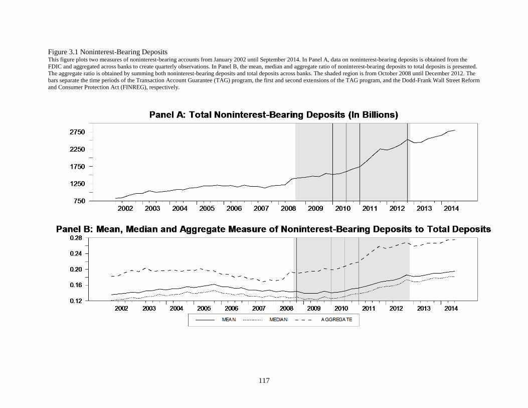
117

Figure 3.1 Noninterest-Bearing Deposits This figure plots two measures of noninterest-bearing accounts from January 2002 until September 2014. In Panel A, data on noninterest-bearing deposits is obtained from the

FDIC and aggregated across banks to create quarterly observations. In Panel B, the mean, median and aggregate ratio of noninterest-bearing deposits to total deposits is presented.

The aggregate ratio is obtained by summing both noninterest-bearing deposits and total deposits across banks. The shaded region is from October 2008 until December 2012. The

bars separate the time periods of the Transaction Account Guarantee (TAG) program, the first and second extensions of the TAG program, and the Dodd-Frank Wall Street Reform

and Consumer Protection Act (FINREG), respectively.

118

participate in the extensions of the TAG program and this potentially over states the amount

of fund that were covered by unlimited insurance during this time. I then summarize and

examine some reasons why these firms might not have participated.

The increase in deposits leads one to question where the funds were coming from.

Because noninterest-bearing account are primarily held by businesses, it is assumed that

corporations provided the cash that increased deposits. As companies were holding more

cash and short-term investments, they seemed to value the safety that bank deposits provided.

The Association for Financial Professionals (AFP) reported that in 2012 companies were

keeping 51% of their short-term investments in bank deposits, up from 42% in both 2010 and

2011 (AFP Liquidity Survey). In 2008, companies kept just 25% of their cash in bank

accounts. Thus, one reason for the increased safety and use of deposits by corporations might

have been the unlimited insurance protection for noninterest-bearing transaction accounts.

I examine the cash holding practices of corporations to see if an increase in cash

holdings took place during the time of the unlimited insurance acts. If corporations held more

funds in noninterest-bearing accounts due to the full insurance guarantee, then we should

observe an increase in new funds or a shift in existing funds from other holdings into these

accounts. Figure 3.2 plots several quarterly measures of corporate cash holdings from

January 2002 until September 2014. As in Azar, et al. (2014), I use cash and cash equivalents

as my measure of liquid assets as these are assumed to be noninterest earning or very low

interest earnings assets. In Panel A, the sum of corporate cash holdings across companies is

presented. Cash and cash equivalents have increased since 2002, with a steeper increase

during the time of the full insurance guarantee. In Panel B, the mean, median and aggregate

119

Figure 3.2 Corporate Holdings of Cash and Cash Equivalents This figure is the plot of corporate holdings of cash and cash equivalents from January 2002 until September 2014. Prior to the third quarter of 2009, cash and cash equivalents is

provided by Compustat comprehensively on an annual basis. To arrive at a quarterly measure, I linearly extrapolated the data. After the third quarter of 2009, Compustat provides

the data comprehensively on a quarterly basis. In Panel A, data on cash and cash equivalents is summed across companies to create an aggregate measure of cash per quarter. In

Panel B, the mean, median and aggregate measure of cash and cash equivalents to total assets is presented. The aggregate ratio is obtained by summing both cash and cash

equivalents and total assets across companies. The shaded region is from 2008 until 2012.The bars separate the time periods of the Transaction Account Guarantee (TAG)

Program, the first and second extensions of the TAG program and the Dodd-Frank Wall Street Reform and Consumer Protection Act (FINREG).

120

ratio of cash and cash equivalents to total assets is presented. Again, a slight increase in cash

and cash equivalents is seen during the initial unlimited insurance periods that levels off or

declines during the later periods. Thus, I do document an increase in corporate cash holdings

and further examine whether the increase was due to full insurance protection.

In addition to using univariate analysis, I employ several different empirical methods

and tests to show an increase in noninterest-bearing deposits, a change in corporate cash

holdings, and then try to relate the increase in cash and noninterest-bearing accounts. Since

banks could opt-out of the TAG program upon its passage and at each subsequent extension,

the sample can be divided between banks that provided unlimited insurance and those that

did not. Using a difference-in-differences strategy, I show a significant variation in

noninterest-bearing deposits held between these two groups. Second, the Bai and Perron

(2003) technique is implemented to test for the presence of structural breaks in corporate

cash and cash equivalents and noninterest-bearing accounts. If the Acts had an effect on

corporate cash holding practices, there should be structural breaks in the aforementioned

series around the time each Act was passed. Third, using several regression models I

document no additional increase in funds took place during the times of the Acts when

controlling for the recent recession.

The remainder of the paper is organized as follows: Section 2 provides a more

detailed discussion of the unlimited insurance protection provided by the TAG program and

FINREG. Section 3 discusses the relationship with corporate cash holdings. Section 4

discusses the relevant literature and presents the hypotheses. Section 5 presents the data. In

Section 6, I outline the models and discuss the empirical results and Section 7 concludes.

121

2. FDIC Insurance

The FDIC was established in response to the Great Depression, primarily to re-assure

the public that deposits held in financial institutions were safe, thus preventing future bank

runs. Initially each account was insured up to $2,500, but has been raised over the years to

the current limit of $250,000. During the most recent recession, the federal government

wanted to provide additional reassurance to depositors and on October 13, 2008, the FDIC

enacted the TAG program, which provided unlimited insurance coverage on noninterest-

bearing accounts until December 31, 2009. It was extended twice until June 30, 2010 and

finally December 31, 2010. In addition, FINREG provided unlimited insurance protection for

noninterest-bearing accounts from December 31, 2010 through December 31, 2012. In this

section, I discuss some of the details surrounding the TAG program and FINREG.

2.1 Noninterest-Bearing Accounts

The unlimited insurance for both the TAG program and FINREG was only offered on

noninterest-bearing transaction accounts. Noninterest-bearing transaction accounts are

defined as an account “with respect to which interest is neither accrued nor paid and on

which the insured depository institution does not reserve the right to require advance notice

of an intended withdrawal.”67

Full insurance was provided on noninterest-bearing accounts because they are held

primarily by corporations and governments for transaction purposes due to Regulation Q.

Regulation Q, which was established in 1933, prohibited banks from paying interest on

67

The definition can be found at https://www.fdic.gov/regulations/resources/TLGP/faq.html#cost.

122

business checking accounts.68

While some individuals might choose to forgo interest and

hold these accounts, it is assumed that they are primarily held by businesses. In its 2009

Annual Report, Regions Financial Corporation confirmed that an increase in funds was not

due to individuals, citing that an increase in noninterest-bearing deposits of $4.7 billion was

driven by an increase in noninterest-bearing deposits from commercial and small businesses

(73).

However, it could be that the increase in noninterest-bearing accounts are not just

from corporations increasing the holdings in these accounts, but individuals moving funds

from interest-bearing accounts to noninterest-bearing accounts. While this would imply that

the individual was forgoing potential interest, the benefit of having the funds fully insured

might have drawn individuals to these accounts. In Figure 3.3, I present evidence that this is

probably not the case and show that an increase in interest-bearing accounts took place

during the time periods of unlimited insurance. This increase, while not as large as the

increase in noninterest-bearing accounts, suggests that bank customers were not just

withdrawing funds and placing them in noninterest-bearing accounts.

Table 3.1 displays the mean, median, and aggregate measure of noninterest-bearing

deposits to total deposits and the total noninterest-bearing deposits each quarter from 2002

until the third quarter of 2014. The time frame for the TAG program is shaded in light grey

and the FINREG period is shaded in dark grey. An increase across all measures is seen over

the entire period of unlimited insurance with a dramatic increase occurring during FINREG.

68

In response to Regulation Q, banks also created other types of bank accounts, such as earning credit-rate accounts,

in order to circumvent this restriction. Earning credit-rate accounts are checking accounts that waive fees or provide

fee-reducing credits to the customer based on the balance of the accounts. Instead of the companies earning interest

on the balance in the accounts, credits are earned that are used to pay down bank fees. The TAG program and

FINREG both included these accounts as noninterest-bearing checking accounts.

123

Figure 3.3 Interest-Bearing Accounts (in Billions) This figure plots interest-bearing deposits from January 2002 until September 2014. Data on interest-bearing deposits is obtained

from the FDIC and aggregated across banks to create quarterly observations. The shaded region is from October 2008 until

December 2012. This is during the time of the Transaction Account Guarantee (TAG) program, the first and second extension to

the TAG program, and the Dodd-Frank Wall Street Reform and Consumer Protection Act (FINREG), respectively.

The final two rows test for a trend over the entire period and a trend over the period

that was covered by unlimited insurance. Both periods show a positive and significant trend

displaying that noninterest-bearing accounts did become a greater fraction of total deposits

over time. The trend is even larger and still statistically significant at a 1% level when

focusing just on the period of unlimited insurance. So while there seems to have been an

increase in noninterest-bearing deposits since 2002, the increase was further exaggerated

during the time of unlimited insurance protection. It is interesting to note that despite the end

of the FINREG unlimited insurance guarantee in 2012, noninterest-bearing deposits have

continued to grow. This will be discussed later in the paper.

2002 2004 2006 2008 2010 2012 20143500

4000

4500

5000

5500

6000

6500

7000

7500

124

Table 3.1 Noninterest-Bearing Accounts Over Time The quarterly aggregate, mean, and median ratio of noninterest-bearing deposits to total deposits and the aggregate, mean, and

median measure of noninterest-bearing deposits is recorded from 2002 until the third quarter of 2014 for all domestic banks. In

addition, a trend is tested. The trend was assigned a value of one in the first quarter of 2002 until 51 in the third quarter of 2014.

The light grey region is the period covered by the TAG program and the dark grey region is the period covered by the FINREG.

Noninterest-Bearing Deposits

to Total Deposits Noninterest-Bearing Deposits

Time Obs. Mean Median Agg. Mean Median Agg.

2002:1 9517 0.1356 0.1214 0.1818

86841 8805 825080537

2002:2 9462 0.1375 0.1229 0.1838

89157 9049 842174744

2002:3 9411 0.1392 0.1245 0.1917

96910 9374 910466291

2002:4 9351 0.1419 0.1287 0.1974

103148 9783 962989218

2003:1 9310 0.1404 0.1258 0.1942

104316 9895 969615406

2003:2 9264 0.1453 0.1303 0.2035

113019 10446 1045426674

2003:3 9232 0.1460 0.1312 0.1948

108375 10533 998999420

2003:4 9176 0.1499 0.1364 0.1967

111253 11090 1019412725

2004:1 9111 0.1479 0.1331 0.1962

114604 11017 1042665277

2004:2 9073 0.1510 0.1357 0.1989

119038 11393 1078603024

2004:3 9019 0.1514 0.1368 0.1946

119315 11477 1074666947

2004:4 8971 0.1561 0.1428 0.1976

125272 12195 1122312083

2005:1 8926 0.1536 0.1386 0.1968

127666 12045 1138013354

2005:2 8863 0.1563 0.1403 0.2015

133859 12364 1184782178

2005:3 8853 0.1593 0.1428 0.1968

133987 12740 1184576367

2005:4 8828 0.1620 0.1464 0.1959

137191 13466 1209475064

2006:1 8785 0.1563 0.1400 0.1879

134596 13125 1180807220

2006:2 8771 0.1555 0.1383 0.1872

136520 13250 1195913113

2006:3 8737 0.1517 0.1347 0.1795

132251 12945 1154021702

2006:4 8673 0.1529 0.1386 0.1837

139652 13445 1209665614

2007:1 8642 0.1474 0.1316 0.1756

135165 13013 1166609472

2007:2 8606 0.1474 0.1314 0.1760

135931 13047 1168459862

2007:3 8551 0.1444 0.1288 0.1681

131637 12713 1124314218

2007:4 8526 0.1473 0.1332 0.1731

139404 13299 1187167398

2008:1 8487 0.1429 0.1283 0.1711

141631 13199 1200601937

2008:2 8444 0.1454 0.1309 0.1750

144672 13477 1220167220

2008:3 8375 0.1425 0.1274 0.1939

166073 13284 1389367353

2008:4 8297 0.1441 0.1297 0.1903 170873 13649 1416198766

2009:1 8239 0.1397 0.1242 0.1918 174443 13507 1435666368

2009:2 8187 0.1395 0.1248 0.1957 179490 13658 1467865302

2009:3 8091 0.1391 0.1235 0.1941 180112 13677 1455663119

2009:4 8004 0.1446 0.1306 0.2021 193260 14814 1545112651

2010:1 7926 0.1405 0.1256 0.1987 191777 14375 1518295841

2010:2 7825 0.1419 0.1272 0.2017 196902 14691 1538982943

2010:3 7756 0.1449 0.1310 0.2077 206484 15226 1599627339

125


Noninterest-Bearing Deposits

to Total Deposits Noninterest-Bearing Deposits

Time Obs. Mean Median Agg Mean Median Agg

2010:4 7653 0.1504 0.1363 0.2146 219984 16110 1681559477

2011:1 7570 0.1525 0.1383 0.2186 230003 16364 1739050987

2011:2 7509 0.1568 0.1410 0.2324 253890 16777 1904171229

2011:3 7433 0.1616 0.1467 0.2460 280827 17727 2084860566

2011:4 7353 0.1673 0.1542 0.2585 307269 18964 2256582626

2012:1 7304 0.1703 0.1566 0.2528 304819 19821 2223653215

2012:2 7241 0.1723 0.1580 0.2576 316490 19930 2288856969

2012:3 7177 0.1770 0.1630 0.2638 332518 20590 2383488887

2012:4 7080 0.1858 0.1741 0.2687 358095 22460 2532090831

2013:1 7016 0.1817 0.1686 0.2589

347474 22135 2434748689

2013:2 6937 0.1829 0.1688 0.2611

353266 22212 2447427187

2013:3 6888 0.1864 0.1737 0.2662

370738 22817 2550303361

2013:4 6809 0.1905 0.1784 0.2665

382971 23829 2604199584

2014:1 6727 0.1903 0.1772 0.2673

394352 24114 2649254580

2014:2 6653 0.1931 0.1808 0.2749

415827 24463 2762753106

2014:3 6586 0.1952 0.1819 0.2754

425479 24945 2798375503

2002:1 -2014:3

0.1560 0.1415 0.2110

198996 15045 1551473402

2008:4-2012:4

0.1546 0.1403 0.2232

241014 16608 1827748653

Entire Trend

0.00*** 0.00*** 0.00***

6215.6*** 283*** 37100000***

P-Value

0.0000 0.0000 0.0000

0.0000 0.0000 0.0000

Unlimited Insurance Trend

0.00*** 0.00*** 0.00***

12035.6*** 540*** 72900000***

P-Value 0.0000 0.0000 0.0000 0.0000 0.0000 0.0000

2.2 Bank Participation

Under the TAG program, banks could voluntarily opt-out of the program. Once a

bank opted-out from the TAG program, it was excluded through each extension of the

program. Bank participation in the program was voluntary because the insurance was funded

by an annual fee paid by each bank. The fee was 10 basis points on any amount over the

deposit insurance limit from October 13, 2008 until December 31, 2009. However, during the

first and second extensions of the program the fee system was increased from 10 basis points

126

to 15-25 basis points, depending on the Risk Category assigned to an entity in the FDIC’s

risk-based premium system.69

By December 31, 2010, 2,077 banks had opted-out of the program: 1,110 banks

opted-out from the original TAG program, 525 opted-out from the first extension, and 442

opted-out from the second extension.70

Statistics on bank participation are provided in Table

3.2. The statistics are separated by the size of the institutions and participation in the program

from the fourth quarter of 2008 until the fourth quarter of 2010. First, the participation of the

two size groups is examined. The participation of smaller institutions remained very high

throughout the periods. For institutions with assets less than $10 billion, the percent of banks

participating in the first quarter of full insurance is 86.55% and declines to 74.71% in the

fourth quarter of 2010. Institutions with assets greater than $10 billion had a very high

participation rate of 93% during the initial periods of the program. The participation rate then

falls to 62.14% during the first extension and around 30% during the final extension. This

high participation rate of large institutions in the initial quarters shows that these banks

judged the benefits of the program to outweigh the fees in the initial periods; however, the

large decline in participation demonstrates that something caused the banks to reevaluate the

benefits of the program.

The noticeable decline in large banks is very interesting and could potentially bias the

effect that the TAG program had on banks. Figure 3.4 plots the sum of noninterest-bearing

deposits for banks that participated in the TAG program. A large decrease in the sum of

noninterest-bearing accounts covered by the program is observed during 2010. This shows

69

Banks in Risk Category I were charged an annual fee of 15 basis points on their noninterest-bearing accounts

above the $250,000 limit. Banks in Risk Category II paid 20 basis points and banks in Risk Categories III and IV

paid 25 basis points. 70

The opt-out lists are provided online at http://www.fdic.gov/regulations/resources/TLGP/optout.html.

127

Table 3.2 Statistics on Banks Participating in the Transaction Account Guarantee Program By Size The table presents statistics on depository institutions split by bank assets and participation in the TAG program each quarter. Participants are banks that participated in the TAG

program and Non-Participants are banks that opted out. Obs. is the number of observations each quarter for each category. Percent of Deposits is the percentage of deposits that

the category makes up of all noninterest-bearing deposits each quarter. Percent Participating is the percentage of each asset group that participated in the TAG program.

Depositary Institutions with Assets ≤ $10 Billion Depositary Institutions with Assets > $10 Billion

Participants

Non-

Participants Participants

Non-Participants

Time Obs.

Percent

of

Deposits Obs.

Percent

of

Deposits

Percent

Participating Obs.

Percent

of

Deposits Obs.

Percent

of

Deposits

Percent

Participating

2008:4

7084 19.67%

1101 0.87%

86.55%

105 79.39%

7 0.08%

93.75%

2009:1

7023 19.58%

1103 0.88%

86.43%

106 79.44%

7 0.09%

93.81%

2009:2

6972 19.38%

1101 0.83%

86.36%

107 79.68%

7 0.11%

93.86%

2009:3

6885 19.51%

1097 0.81%

86.26%

102 79.58%

7 0.09%

93.58%

2009:4

6809 19.13%

1091 0.83%

86.19%

96 79.94%

8 0.09%

92.31%

2010:1

6260 17.70%

1563 2.23%

80.02%

64 17.99%

39 62.08%

62.14%

2010:2

6170 17.32%

1552 2.15%

79.90%

64 17.85%

39 62.68%

62.14%

2010:3

5700 15.11%

1948 3.95%

74.53%

34 3.99%

74 76.95%

31.48%

2010:4 5638 15.09% 1909 3.84% 74.71% 32 3.85% 74 77.22% 30.19%

128

the effect that the large banks had when they withdrew from the program. It also implies that

the amount of noninterest-bearing deposits covered by the unlimited insurance was not as

extensive at the end of the TAG program as one might have believed. Table 3.2 also presents

the percent of total noninterest-bearing deposits that the participating and non-participating

banks’ composed based on size. It is seen that even though several thousand small

institutions participated in the program, they composed less than 20% of all total noninterest-

bearing deposits. On the other hand, despite the initial participation of only 105 large

institutions, they held 79% of all noninterest-bearing deposits. After the extensions this

measure drops to 18% and 4% during the first and second extensions of unlimited insurance,

respectively. Thus, there is a need to control for firms exiting the program when examining

the effect of the TAG program.

Figure 3.4 Noninterest-Bearing Deposits for Banks that Participated in the TAG Program This figure presents data (in Billions) on the sum of noninterest-bearing deposits for banks that participated in the TAG program

from January 2002 until September 2014. The shaded region is from October 2008 until December 2012. The bars separate the

time periods of the Transaction Account Guarantee (TAG) Program, the first and second extensions of the TAG program and the

Dodd-Frank Wall Street Reform and Consumer Protection Act (FINREG).

2002 2004 2006 2008 2010 2012 20140

500

1000

1500

2000

2500

3000

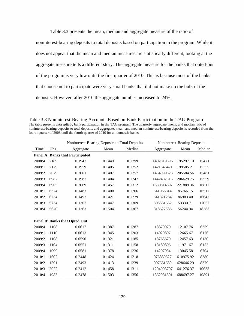
129

Table 3.3 presents the mean, median and aggregate measure of the ratio of

noninterest-bearing deposits to total deposits based on participation in the program. While it

does not appear that the mean and median measures are statistically different, looking at the

aggregate measure tells a different story. The aggregate measure for the banks that opted-out

of the program is very low until the first quarter of 2010. This is because most of the banks

that choose not to participate were very small banks that did not make up the bulk of the

deposits. However, after 2010 the aggregate number increased to 24%.

Table 3.3 Noninterest-Bearing Accounts Based on Bank Participation in the TAG Program The table presents data split by bank participation in the TAG program. The quarterly aggregate, mean, and median ratio of

noninterest-bearing deposits to total deposits and aggregate, mean, and median noninterest-bearing deposits is recorded from the

fourth quarter of 2008 until the fourth quarter of 2010 for all domestic banks.

Noninterest-Bearing Deposits to Total Deposits Noninterest-Bearing Deposits

Time Obs. Aggregate Mean Median Aggregate Mean Median

Panel A: Banks that Participated

2008:4 7189

0.1942 0.1449 0.1299

1402819696 195297.19 15471

2009:1 7129

0.1959 0.1405 0.1252

1421645471 199585.21 15355

2009:2 7079

0.2001 0.1407 0.1257

1454099623 205584.56 15481

2009:3 6987

0.1987 0.1404 0.1247

1442482313 206629.75 15559

2009:4 6905

0.2069 0.1457 0.1312

1530814697 221889.36 16812

2010:1 6324

0.1483 0.1400 0.1266

541956314 85766.15 16517

2010:2 6234

0.1492 0.1421 0.1279

541321284 86903.40 16642

2010:3 5734

0.1307 0.1447 0.1309

305531632 53330.71 17057

2010:4 5670

0.1363 0.1504 0.1367

318627586 56244.94 18383

Panel B: Banks that Opted Out

2008:4 1108

0.0617 0.1387 0.1287

13379070 12107.76 6359

2009:1 1110

0.0613 0.1345 0.1203

14020897 12665.67 6126

2009:2 1108

0.0590 0.1321 0.1185

13765679 12457.63 6130

2009:3 1104

0.0551 0.1311 0.1158

13180806 11971.67 6153

2009:4 1099

0.0581 0.1378 0.1236

14297954 13045.58 6704

2010:1 1602

0.2448 0.1424 0.1218

976339527 610975.92 8380

2010:2 1591

0.2493 0.1413 0.1239

997661659 628646.29 8379

2010:3 2022

0.2412 0.1458 0.1311

1294095707 641276.37 10633

2010:4 1983 0.2478 0.1503 0.1356 1362931891 688697.27 10891

130

While an exact reason why some banks opted-out of the TAG program is unknown

and can vary by institution, I provide a summary of reasons. The first explanation is the

increased fees paid on deposits above the insurance limit during the extensions. Fees

increased for all banks that stayed in the program, but were higher for banks within worse

risk categories. If the withdrawal of large banks from the program is the results of increased

fees it could be that 1) these banks were in worse risk categories and it would cost them more

or 2) management judged the bank to be in a good financial position and did not elect to pay

the increased fee. If the increase in large banks withdrawing from the program in early 2010

is due to larger fees paid, it would be prudent to look at the differences in risk between the

banks that opted-out of the program and banks that remained in the program.

The official Risk Categories used by the FDIC are not released for the safety of the

banks. The Risk Categories are calculated by comparing the capital category of the bank and

the supervisory group ratings. For this paper, the analysis on Risk Category examines just the

capital categories (capital ratios) and not the supervisory groups. Capital ratio statistics are

presented for small banks in Table 3.4 and for large banks in Table 3.5. In Panel A of both

tables, I compare the mean and median risk ratios of the banks that participated and the banks

that did not participate in the initial TAG program. Panel B presents the risk ratios for firms

that exited during the first extension of the program and Panel C presents the risk ratios for

firms that exited during the second extension of the program. The dates for the first and

second extension do include the previous quarter, as this is the quarter banks had to decide

whether to participate or not, making capital measures important during this quarter, as well.

131

Table 3.4 Capital Ratios for Small Banks The table presents capital ratios on small banks (assets less than $10 billion) based on participation in the TAG program. Number is the total number of institutions eligible for the

act or extension. Thus, the total number of entities in Panel B and C takes into account that banks that opted-out of the program in December 2008 were not eligible to participate

in the extension.

Panel A: Risk Ratios for Initial Firms that Opted-Out

Participating Firms Non-Participating Firms

Number Risk Ratio Number Risk Ratio Difference

P-Value

2008:4 - 2010:4 Core Capital (Leverage) Ratio Mean 7096 10.5284 1098 13.2413 -2.7129 *** 0.0000

Median 7096 9.2616 1098 10.7959 -1.5342 *** 0.0000

Tier 1 Risk-Based Capital Ratio Mean 7096 18.9928 1098 26.1260 -7.1333 *** 0.0000

Median 7096 13.0382 1098 17.8263 -4.7881 *** 0.0000

Total Risk-Based Capital Ratio Mean 7096 20.1432 1098 27.1282 -6.9850 *** 0.0000

Median 7096 14.2039 1098 18.8545 -4.6506 *** 0.0000

Panel B: Risk Ratios for Firms that Opted-Out of the First Extension



P-Value


Median 6342 9.2673 478 9.4813 -0.2140 *** 0.0002

Tier 1 Risk-Based Capital Ratio Mean 6342 17.2742 478 44.1103 -26.8361 ** 0.0172

Median 6342 13.2583 478 14.4071 -1.1488 *** 0.0000

Total Risk-Based Capital Ratio Mean 6342 18.4529 478 45.2216 -26.7686 ** 0.0173

Median 6342 14.4458 478 15.5332 -1.0873 *** 0.0000

Panel C: Risk Ratios for Firms that Opted-Out of the Second Extension



P-Value


Median 5769 9.3201 408 9.4779 -0.1578 ** 0.0167


Median 5769 13.4521 408 14.1573 -0.7053 *** 0.0030


Median 5769 14.6312 408 15.3275 -0.6963 *** 0.0063

132

significantly different from zero for all measures and time periods. There is varying statistical

significance from a 5% level to a 1% level. Interestingly, banks that exited have larger ratios

suggesting they are in better Risk Categories. So, it seems that the small banks that decided

not to participate in the program and its extensions had better capital ratio positions than the

In Table 3.4, the difference between the Core Capital Ratio, the Tier 1 Risk-Based Capital

Ratio, and the Total Risk-Based Capital Ratio for small banks are negative and banks that

elected to stay in, which means that these banks may have judged themselves to not be at a

high risk of failure and in need of extra insurance. Also, the additional expense for the

insurance may have been enough to drive banks to exit if they did not feel there was a great

need for it.

In Table 3.5, the difference between the capital measures presents a different story for

large banks. During the initial periods of the TAG program, most measures do show that the

large banks that exited had larger capital ratios, with the exception of a lower Tier 1 Risk-

Based Capital Ratio measured by mean and Total Risk-Based Capital Ratio as measured by

the mean. During the first extension, the banks that exited the program have a smaller mean

and median capital ratio than the banks that participated. So it is possible that some of these

banks might have exited because of increased fees based on capital risk, but both the mean

and median measures are still large. During the final extension, the measures again differ,

depending upon whether the median or mean is used. The mean suggests that the banks that

exited had higher risk ratios while the median suggests they had lower risk ratios.

Another explanation is that the banks judged themselves to not need the reassurance

of fully insured deposits and thus choose not to pay the increased fees. I contacted several of

the banks that withdrew from the program for the final extension and they cited that they

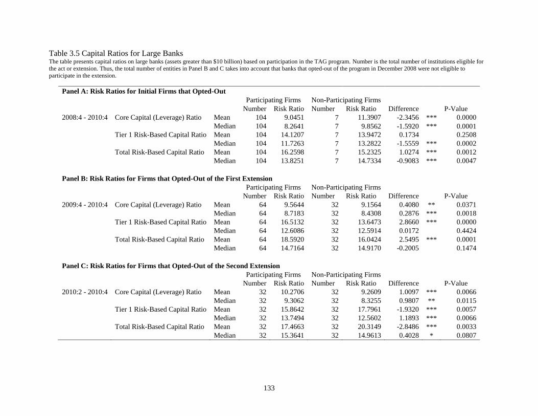
133

Table 3.5 Capital Ratios for Large Banks The table presents capital ratios on large banks (assets greater than $10 billion) based on participation in the TAG program. Number is the total number of institutions eligible for

the act or extension. Thus, the total number of entities in Panel B and C takes into account that banks that opted-out of the program in December 2008 were not eligible to

participate in the extension.

Panel A: Risk Ratios for Initial Firms that Opted-Out



P-Value


Median 104 8.2641 7 9.8562 -1.5920 *** 0.0001

Tier 1 Risk-Based Capital Ratio Mean 104 14.1207 7 13.9472 0.1734

0.2508

Median 104 11.7263 7 13.2822 -1.5559 *** 0.0002

Total Risk-Based Capital Ratio Mean 104 16.2598 7 15.2325 1.0274 *** 0.0012

Median 104 13.8251 7 14.7334 -0.9083 *** 0.0047

Panel B: Risk Ratios for Firms that Opted-Out of the First Extension



P-Value

2009:4 - 2010:4 Core Capital (Leverage) Ratio Mean 64 9.5644 32 9.1564 0.4080 ** 0.0371

Median 64 8.7183 32 8.4308 0.2876 *** 0.0018

Tier 1 Risk-Based Capital Ratio Mean 64 16.5132 32 13.6473 2.8660 *** 0.0000

Median 64 12.6086 32 12.5914 0.0172

0.4424

Total Risk-Based Capital Ratio Mean 64 18.5920 32 16.0424 2.5495 *** 0.0001

Median 64 14.7164 32 14.9170 -0.2005

0.1474

Panel C: Risk Ratios for Firms that Opted-Out of the Second Extension



P-Value

2010:2 - 2010:4 Core Capital (Leverage) Ratio Mean 32 10.2706 32 9.2609 1.0097 *** 0.0066

Median 32 9.3062 32 8.3255 0.9807 ** 0.0115


Median 32 13.7494 32 12.5602 1.1893 *** 0.0066


Median 32 15.3641 32 14.9613 0.4028 * 0.0807

134

chose to withdraw from the program because they felt the clientele no longer needed

assurance that the banks were financially stable. Another reason for the withdrawal could

have been that the large banks did not want the stigma that came with being involved in a

program that was intended to restore confidence. One final explanation for the decline in

large banks is that the Dodd-Frank Act discussed extending the unlimited insurance past the

2010 deadline and it did so with no additional costs for the companies. Thus, the large banks

may have seen an opportunity to exit the TAG program and avoid paying fees on deposits for

one year to six months until the Dodd-Frank Act took effect. Regions Financial Corporation,

one company that opted-out of the second extension, cites in the 2011 Annual Report that the

“decision to exit the program did not have a significant impact on liquidity (98).”

2.3 Repeal of Regulation Q

One concern regarding FINREG is the repeal of Regulation Q, thus allowing

corporations to earn interest on transaction accounts. The concurrent events of allowing

corporations to have interest-bearing accounts but unlimited insurance on noninterest-bearing

accounts forced companies to balance the additional benefit of the unlimited insurance with

the benefit of interest earned on checking accounts. Due to the low interest rate environment,

most companies choose the additional benefit of the insurance over the interest accounts. The

2011 AFP Liquidity Survey also found that only 16% of companies surveyed were looking

into switching to interest-bearing accounts and 29% were currently exploring the options

with banks while 50% of companies had no plan to switch. In 2011, Citi claimed that in

response to low interest rates and unlimited insurance, only 1- 2% of companies were

expected to shift to interest bearing accounts (Kelly (2011)). Moreover, Citi claimed that

135

when interest rates begin to rise, companies might have more of an incentive to transfer funds

to accounts that pay interest. Dub Newman of Bank of America stated “to the degree that a

client is focused on [unlimited FDIC insurance], particularly in a low-interest rate

environment where they’re not seeing a lot of return regardless of the instrument they’re in,

that extra safety of FDIC [coverage] has a value to it (Kelly (2011)).”

2.4 Expiration of the Unlimited Insurance

Section 343 of the Dodd-Frank Act expired on December 31, 2012. Some industry

groups such as the Independent Community Bankers of America and the American Bankers

Association asked lawmakers to extend the unlimited guarantee, but the extension did not

occur.71,72

In January 2013, Bloomberg reported that clients of large U.S. banks withdrew

funds at the fastest weekly rate since September 11, 2001 stating that “what you are seeing

now is probably TAG [program] money.”73

While it remains to be seen what companies plan

to do with the additional funds over the next few years, the 2012 AFP Liquidity Survey

found that 60% of companies said they had no plans to reduce cash balances in bank deposits

upon termination of the FINREG provision. In addition, the FDIC (2013) reported that

balances in domestic noninterest-bearing accounts increased by $149.1 billion during the

fourth quarter of 2012 and a third of this increase ($49.5 billion) was in balances in

noninterest-bearing accounts above the $250,000 insurance limit. In March 2013, the FDIC

71

Vipal Monga, “Cash-Haven Clock Is Ticking,” The Wall Street Journal, September 18, 2012. 72

As of November 9, 2012 the FDIC posted a PDF document on their website stating that Section 343 of the Frank-

Dodd Act was set to expire on December 31, 2012 and deposits held at FDIC insured institutions would only be

insured up to $250,000. This can be found at: http://www.fdic.gov/deposit/deposits/unlimited/expiration.pdf. On

December 13, 2012 the U.S. Senate blocked a vote to extend the unlimited insurance on noninterest-bearing

accounts. 73

Dakin Campbell, “U.S. Bank Deposits Drop Most Since 9/11 Terror Attacks,” Bloomberg, January 23, 2013

136

reported a decline in noninterest-bearing accounts of $70 billion, but this represented only

5% of funds held in noninterest-bearing accounts.

In Figure 3.1, I document a decline in noninterest-bearing deposits and the ratio of

noninterest-bearing deposits to total deposits across all banks during the first half of 2013.

However, this was followed by an increase in the accounts to levels at and even above the

last quarter of unlimited insurance. So, while it appears that a drawdown of funds might have

occurred after the expiration of Section 343, the amounts held in these accounts do continue

to rise despite the lower insurance limit.

3. Corporate Cash Holdings

The documented increase in noninterest-bearing accounts over the time of the

unlimited insurance periods leads one to next look into whether companies provided the

increase in funds. It is natural to believe that the funds came from companies, as they are the

primary holder of noninterest-bearing accounts. I will primarily examine corporate cash

holdings as the reason for the increase in noninterest-bearing deposits since these firms are

publicly held and report holdings of cash and cash equivalents. I do recognize that smaller

corporations and privately held corporations may have also increased cash holdings and

contributed to the increase in noninterest-bearing accounts, but data limitations prevent a

fuller analysis that includes these companies.

Two explanations are possible for the increase in bank accounts funds. Corporations

could have increased holdings in noninterest-bearing bank accounts, but did so by simply

shifting funds from other assets into these accounts. Alternatively, they could have directly

increased cash held in these accounts. Figure 3.5 looks at the former of these events. I plot

137

the sum of cash and cash equivalents across all corporations with available information in

Compustat as well as the sum of short-term investments that these corporations held. As in

Azar, et al. (2014), I assume that cash and cash equivalents is a nonearning or low interest

earning asset and short-term investments are all short-term interest earning investments that

corporations hold.74

For simplicity, I will refer to cash and cash equivalents simply as cash

for the remainder of the paper. In Panel A, both cash and short-term investment increased

during periods of full insurance coverage for corporations. A decline in investments is

observed prior to the financial crisis however, cash seems to stay constant leading up to the

unlimited insurance periods. In Panel B, the aggregate ratio of cash to total assets is plotted

with the aggregate ratio of short-term investments to total assets. This panel shows a decline

in the ratio of investments prior to the financial crisis, but an increase during the periods of

full insurance protection. The cash holdings ratio increases slightly during initial periods and

seems to level off during the first extension. Figure 3.5 shows that overall, corporations did

not pull short-term investments to hold in the form of cash, but increased both types of

holdings.

While I do not have direct numbers relaying how much each individual company is

holdings in noninterest-bearing accounts, I am able to use the Flow of Funds as an

approximation for the types of investments corporations were holdings during the increased

insurance guarantees. In Figure 3.6, I look into whether nonfinancial corporate firms

74

Cash and cash equivalents is defined by Compustat to include: bank drafts, banker’s acceptances, cash, certificates

of deposit included in cash by the company, check (cashiers or certified), demand certificates of deposit, demand

deposits, letters of credit, and money orders. Short-term investments includes: accrued interest combined with short-

term investments, brokerage firms’ good faith and clearing-house deposits, cash in escrow, cash segregated under

federal and other regulations, certificates of deposit included in short-term investments by the company, certificates

of deposit as reported as a separate item in current assets, commercial paper, gas transmission companies’ special

deposits, government and other marketable securities, marginal deposits on commodity futures contracts, marketable

securities, money-market funds, repurchase agreements shown as current assets, real estate investment trust shares

of beneficial interest, restricted cash shown as a current asset, term deposits, time deposits and time certificates of

deposit (savings accounts shown in current assets), and Treasury bills listed as short-term.

138

Figure 3.5 Cash and Cash Equivalents and Short-term Investments This figure presents data on corporate holdings of cash and cash equivalents and short-term investments from January 2002 until September 2013. Data on cash and cash

equivalents and short term investments is obtained from Compustat. It is provided on an annual basis, but linear extrapolated for a quarterly measure. Data is given for each

company and then summed across companies to create an aggregate measure of cash per quarter. The shaded region is from 2008 until 2012. The bars separate the time periods of

the Transaction Account Guarantee (TAG) Program, the first and second extensions of the TAG program and the Dodd-Frank Wall Street Reform and Consumer Protection Act

(FINREG).

139

Figure 3.6 Liquid Assets Held by Nonfinancial Corporations This figure presents data on the amount of liquid assets held by nonfinancial corporate businesses from January 2002 until September 2014. Data is obtained from the Flow of

Funds account L.102. The Other category is the sum of security repurchase agreements, credit market instruments, commercial paper, treasury securities, agency-and GSE- backed

securities, and municipal securities and loans. The shaded region is from 2008 until 2012. The bars separate the time periods of the Transaction Account Guarantee (TAG)

Program, the first and second extensions of the TAG program and the Dodd-Frank Wall Street Reform and Consumer Protection Act (FINREG).

140

increased amounts in checkable deposit accounts.75

This data comes from the Flow of Funds

account L.102, which breaks down the assets of nonfinancial corporations into several

categories: checkable deposits, time and savings deposits, money market mutual funds, and

others.76

While checkable deposits may include other accounts than noninterest-bearing

transaction accounts, the majority of funds covered in the checkable deposits classification

for corporate nonfinancial businesses would be noninterest-bearing accounts. Checkable

deposits experienced a large decline prior to the passage of the TAG program followed by a

sharp increase during the initial periods of the unlimited insurance. These deposits appeared

to level off during the FINREG period. The increase from the third quarter of 2008 until the

end of the unlimited insurance in the fourth quarter of 2010 represents a 205.8% increase.

This is an extremely large increase even though according to the graph corporations hold

fewer assets in this category. The bulk of the increase (178.6%) took place during the

original TAG program. So it seems that corporations adjusted their holdings in checkable

deposits during the initial insurance increase and then held the levels steady during FINREG.

In looking at the other asset categories, there is a large increase in money market mutual

funds prior to the passage of the TAG program and then a sharp decline beginning in the

fourth quarter of 2008. Time and savings deposits experience a large increase in funds during

the time of the unlimited insurance guarantees as well, even though these assets were not

guaranteed, as they paid interest on deposits held in the accounts. The other category does

75

In Appendix Figure A.3.1, I plot the asset holdings for all nonfinancial business. I document an increase in these

firms’ checkable deposits, but it is not as large as the increase in corporate cash in checkable deposits. I do want to

mention that these firms held more in checkable deposits than some other asset categories as opposed to corporate

firms. 76

The Others category refers to other interest bearing assets that companies hold such as security repurchase

agreements, credit market instruments, commercial paper, treasury securities, agency-and GSE- backed securities,

and municipal securities and loans.

141

not seem to fluctuate much, but declines slightly throughout the period of unlimited

guarantees.

One concern is that the increase in insurance is taking place during the most recent

financial crisis. In the academic literature, cash holdings have been shown to vary during

business cycles. In particular it seems that cash holdings decline during expansions and

increase during recessions (Almeida, et al. (2004), Ferreira, et al. (2005), Baum, et al. (2006),

Duchin, et al. (2010), and Stone and Gup (2014)). Separating the effect of the unlimited

insurance from the recessionary periods is examined in a later section.

In conclusion, while I do not have direct evidence that companies placed funds in

bank accounts during the financial crisis, I have shown that companies did not seem to

decrease holdings in short-term investments to move funds into these accounts and it appears

that they increased the amounts held in checkable deposits. Thus, I proceed with an empirical

examination of the analysis of cash holdings and noninterest-bearing deposits during this

time.

4. Literature Review and Hypotheses

This section discusses the relevant literature and the hypothesis that the paper

develops.

4.1 Literature Review

Since the unlimited insurance provisions of the TAG program and FINREG are very

rarely examined in academic literature, the majority of the discussion surrounding the Acts

has come from banks and Congress. Bank of America and Goldman Sachs have both

142

published reports discussing the implications of full insurance.77

Schich (2008) also provides

a good summary of the full insurance guarantee and the implications for extending the

insurance that was presented to the OECD’s Committee on Financial Markets on November

13, 2008. Pozar (2011) discussed the Dodd-Frank Act and the effect of institutional cash

pools. He further discussed the increase in temporary unlimited insurance on noninterest-

bearing transactions and how companies were not expected to increase cash pools past levels

held in July 2011. Hoskins (2012) discusses the unlimited insurance guarantees and the

potential impact upon its expiration. However, no empirical tests are provided in any of the

discussions.

To my knowledge, no one has directly examined the effect of FDIC insurance on

corporate liquidity. Academic research on FDIC insurance has primarily examined the

insufficient funding of the FDIC Bank Insurance Fund (Merton (1977), Marcus and Shaked

(1984), and Kuritzkes, et al. (2005)). Pennacchi (2006) presented empirical evidence that

banks have become better at managing liquidity shocks since the advent of FDIC insurance.

In addition, he stated that the flight to bank deposits may be explained by the FDIC

insurance.

Some papers have focused on the increase in cash holdings over the years, but none

have directly related the increase to the unlimited insurance environment. The most extensive

work has addressed balance sheet determinants and corporate cash holdings. Opler, et al.

(1999) studied balance sheet determinants of the firm. They documented that firms with

strong growth opportunities and riskier activities hold relatively more cash. They also found

77

Goldman Sachs Research Department published “ US Daily: FDIC Deposit Guarantees: Another Year-End Risk”

on September 4, 2012. It is available at: http://www.goldmansachs.com/gsam/pdfs/GLM/research-FDIC-deposit-

guarantees.pdf. Bank of American published “ Life After Full FDIC Insurance” in April 2012. It is available at:

https://corp.bankofamerica.com/documents/10157/67594/LifeAfterFDIC.pdf.

143

that large firms and those with credit ratings tend to hold relatively less cash. Bates, et al.

(2009) documented that from 1980 until 2006, U.S. firms increased cash holdings. They

found increases among firms that either did not pay dividends, were in more recent IPO

listing cohorts, or were in industries that experience the greatest increase in idiosyncratic

volatility. Reasons attributed to this build-up were fallen inventories, increased cash flow

risk, decreased capital expenditures, and increased R&D expenditures. In December 2008,

during the most recent financial crisis, Campello, et al. (2010) surveyed chief financial

officers (CFOs) in 39 countries and found that financially constrained firms planned to cut

more investment, technology, marketing, and employment relative to financially

unconstrained firms. Furthermore, constrained firms had to use cash reserves and cut planned

dividends during the crisis.

4.2 Hypotheses

The goal of this paper is to document the effect of increased insurance protection on

corporate cash balances. This is done by first examining noninterest-bearing deposits and

leads to the following hypotheses:

Hypothesis 1: Banks that participated in the TAG program experienced an increase in

noninterest-bearing deposits. Therefore there should be a significant difference between

the amount of funds held in noninterest-bearing accounts at banks that participated and at

banks that opted-out of the TAG program.

Each extension of the TAG program and the passage of FINREG provided companies

with the confidence that the insurance would last indefinitely. Around the time that each Act

was announced or passed, a significant increase in noninterest-bearing accounts and cash

holdings should occur.

144

Hypothesis 2: Significant breaks in both noninterest-bearing accounts and corporate cash

holdings around the passage of the Acts should be observed.

To analyze the impact of the unlimited insurance Acts on corporate cash holdings, I

am forced to use dummy variables as I do not have the direct holdings of cash in noninterest-

bearing accounts. While the use of the dummy variables for the dates of the TAG program

and FINREG in the company analysis is not ideal, it does capture how cash holdings changed

during the periods of unlimited insurance. In addition, The Great Recession, which lasted

from December 2007 until June 2009, has been shown to have had an effect on cash

holdings. In the corporate analysis, I control for the common cash holdings determinant as

well as recessions.

Hypothesis 3: When controlling for corporate determinants and the business cycle,

corporate cash holdings should increase during the times of the unlimited insurance Acts

if corporations increased cash balances due to the unlimited insurance protection.

5. Data

Quarterly data on bank deposits was gathered from the FDIC call reports from

January 2002 until September 2014. Information is gathered on noninterest-bearing deposits,

interest-bearing deposits, total deposits, and capital ratios for all FDIC insured institutions.

To make the data comparable to the corporate cash holdings data, banks outside of the United

States are deleted.78

Data on corporations was gathered from both Compustat Quarterly files and

Compustat Annual files. Financial firms (SIC 6000-6999) and utilities (SIC 4900-4999) are

excluded because financial firms hold cash related to their unique business practices and

utilities hold cash for regulatory purposes. Because I am trying to match bank data with the

78

The FDIC provides bank data on institutions located in the U.S. territories of American Samoa, Guam, Mariana

Islands, Puerto Rico, and the Virgin Islands. These represent approximately 706 observations. Excluding them in the

data set does not affect the results. These results are available upon request.

145

corporate data as best as possible, I collect quarterly data on commonly used corporate

determinants. The variables that have been chosen are in line with past literature such as in

Opler, et al. (1999). The control variable include: market-to-book ratio, cash flow, net

working capital-to-assets, capital expenditures-to-assets, leverage, R&D-to-sales,

acquisitions-to-assets, dividend dummy, investment grade dummy, size, and cash flow

riskiness.79

The main measure of cash held by corporations used in this paper is cash and

cash equivalents (cash).80

Prior to the third quarter of 2009, cash is reported comprehensively

in the annual database. To make the data comparable, I use linear extrapolation to create

quarterly observations. Past the third quarter of 2009, Compustat reports cash on a quarterly

basis. Thus, if cash is reported quarterly it is used and if not, linear extrapolation is used.

Appendix Figure A.3.2 compares the quarterly measure of cash that is partly interpolated and

the quarterly observations provided in Compustat. A definition of all corporate variables is

given in appendix Table A.3.1.

As a measure of the periods of unlimited insurance I have the following four dummy

variables. TAGP Dummy is a dummy variable that equals one if the date of the quarterly

report covers the original dates of the TAG program from October 14, 2008 until December

31, 2009 and zero otherwise. Since quarterly data is being used this is measured as the fourth

quarter of 2008 until the fourth quarter of 2009. First Extension TAGP Dummy is a dummy

variable that equals one if the date of the quarterly report covers the original dates of the first

79

Capital expenditures and acquisitions are reported on a year-to-date basis in Compustat. To arrive at quarterly

observations, the data is lagged one quarter and the lagged value is subtracted from the current quarterly observation

for quarters 2, 3, and 4. 80

Cash and cash equivalents is defined in detail in footnote 74. This is different from the commonly used measure in

the cash holdings literature: cash, cash equivalents, and short-term investments. Cash, cash equivalents, and short-

term investments is assumed to include interest-bearing assets and cash and cash equivalents is nonearning or low-

interest earnings assets. Since the focus is on noninterest-earning deposits, the best corporate variable that would

capture these accounts with the least interest-earning assets is cash and cash equivalents. Appendix Figure A.3.3

plots the comparisons between the cash, cash equivalents, and marketable securities and the interpolated quarterly

cash and cash equivalents measure.

146

extension of the TAG program from January 1, 2010 until June 30, 2010 and zero otherwise.

This covers the first quarter of 2010 until he second quarter of 2010. Second Extension TAGP

Dummy is a dummy variable that equals one if the date of the quarterly report falls within the

time frame of the second extension of the TAG program from July 1, 2010 until December

31, 2010 or zero otherwise. In quarterly terms, this covers the third quarter of 2010 until the

fourth quarter of 2010. FINREG Dummy is a dummy variable that equals one if the quarterly

report date falls within January 1, 2011 and December 31, 2012 or zero otherwise.81

The

FINREG Dummy covers the first quarter of 2011 until the fourth quarter of 2012.

As mentioned earlier, one concern is that the time period of unlimited insurance falls

during the most recent recession. Thus, it is necessary to control for the recession in the

regression analysis to get a more complete picture of the determinants of cash holdings. To

control for recessions, five additional macroeconomic variables are included that have been

shown to vary over the business cycle. The NBER defines a recession as a significant decline

“visible in real GDP, real income, employment, industrial production, and wholesale-retail

sales.”82

Thus, the civilian-employment to population ratio, industrial production index, and

GDP Gap are included.83

It is expected that during economic turmoil all variables would

decline.84

In addition, the term spread, defined as the difference between the ten-year and

one-year Treasury Constant Maturity Rate, and the default spread, defined as the difference

between Moody’s Aaa corporate bond yield and Moody’s Baa corporate bond yield are

included. It is expected that the term spread would decline during recessions and the default

81

FINREG began on December 31, 2010, the same day that the TAG program ended. FINREG Dummy does not

include December 31, 2010 because that would include the entire quarter ending with December 31, 2010 of which

the majority of the observations were included under the TAG program and not FINREG. 82

NBER “US Business Cycles Expansion and Contractions” http://www.nber.org/cycles/cyclesmain.html 83

GDP Gap is defined as the difference in real GDP and real potential GDP. 84

When it is suggested that a decline in GDP Gap would occur it is implied that the GDP Gap would become

negative and this value would decline further.

147

spread would increase during recessions. The term spread and default spread are included

because it has been shown that each is correlated with recessions. Fama and French (1989)

find that the term spread displays business cycle patterns. Wheelock and Wohar (2009)

provide a literature survey of the term spread and its predictive power with output growth

and recessions across several countries. Chen (1991) confirms that the default spread is

negatively correlated with output growth. All macroeconomic variables and their components

are obtained from the Federal Reserve Economic Data (FRED).

Table 3.6 contains the summary statistics on the corporate control variables,

unlimited insurance dummies, and macroeconomic indicators. In Panel A, the mean of cash

holdings is 0.1457 indicating that companies are holding on average 15% of total assets in

cash. The mean value of cash and short term-investments to assets is slightly higher at

0.1873. So companies are holding on average 4% more short-term investments than cash.

Turning our attention to Panel B, roughly 10% of observations occur during the TAG

program and a little more than 3.5% occur during each extension. More observations occur

during FINREG’s unlimited insurance dummy because it covered nearly twice as long as any

of the other periods.

6. Econometric Models and Empirical Results

6.1 Difference-in-Differences

I first empirically test whether the TAG program had an effect on noninterest-bearing

accounts when it was first enacted. If customers valued the additional insurance provided by

a bank that participated in the TAG program, the bank should have an increase in

148

Table 3.6 Summary Statistics This table represents the summary statistics on key variables for the 2002 through the fourth quarter of 2014 samples for all firms

in Compustat. Cash holdings, the dependent variable, is defined as cash and cash equivalents divided by total assets. Cash and

short term investments to assets is defined as cash, cash equivalents, and short term investments divided by total assets. Market-

to-book ratio is defined as the market value per share to the stated book value of equity. Cashflow is earnings after interest,

dividends and taxes divided by total assets. Net working capital is defined as working capital minus cash and cash equivalents

divided by total assets. Capital expenditure to assets is capital expenditure divided by total assets. Leverage is long term debt

plus current debt divided by total assets. R&D to sales is R&D divided by sales. Acquisitions to assets are acquisitions divided by

total assets. Dividend Dummy is one if the company pays a dividend and zero otherwise. Investment Grade Dummy is set equal to

one if a company has an investment grade short or long term rating, otherwise the dummy equals zero. Size is the natural log of

the firm’s total assets in 2009 dollars. Cash Flow Riskiness is measured as the standard deviation of industry cash flows

computed by the manner suggested in Opler et al. (1999). It is calculated as the standard deviation of cash flows for the previous

five years if available. The average is then taken across the two-digit SIC code. TAGP Dummy is a dummy variable equal to one

if the quarterly report is between October 14, 2008 and December 31, 2009 and zero otherwise. Extension TAGP Dummy is a

dummy variable equal to one if the quarterly report is between January 1, 2010 and June 30, 2010 and zero otherwise. Second

Extension TAGP Dummy is a dummy variable equal to one if the quarterly report is between July 1, 2010 and December 31, 2010

and zero otherwise. FINREG Dummy is a dummy variable equal to one if the quarterly report is between January 1, 2011 and

December 31, 2012 and zero otherwise. The civilian employment to population ratio measures the percentage of the US

population is employed. The industrial production index is an indexed measure of industrial production in the US. GDP Gap is

the difference between real GDP and real potential GDP. Term spread is defined as the difference between the ten-year and one-

year Treasury Constant Maturity Rate. Default spread is defined as the difference between Moody’s Aaa corporate bond yield

and Moody’s Baa corporate bond yield.

Panel A: Corporate Summary Statistics Mean

Standard


Number of

Observations

Cash Holdings 0.1457 0.1817 0 1 164771

Cash and Short-term Investments to

Assets 0.1873 0.2234 0 1 170092

Market to Book 2.9983 5.8816 0.4307 48.8439 170092

Cash Flow -0.0396 0.2236 -1.7351 0.1256 170092

Net Working Capital-to-Assets -0.1312 0.9810 -7.7379 0.5344 170092

Capital Expenditure-to-Assets 0.0124 0.0181 -0.0016 0.1122 170092

Leverage 0.3519 0.5944 0 4.5000 170092

R&D to Sales 0.4455 2.3841 0 20.9037 170092

Acquisitions-to-Assets 0.0045 0.0199 -0.0019 0.1484 170092

Dividend Dummy 0.2105 0.4077 0 1 170092


Size 0.7217 2.5332 -6.1257 6.0069 170092


Panel B: Unlimited Insurance Dummy

Variables Mean

Standard


Number of

Observations

TAGP Dummy 0.0930 0.2904 0 1 170092

Extension TAGP Dummy 0.0373 0.1894 0 1 170092

Second Extension TAGP Dummy 0.0362 0.1868 0 1 170092

FINREG Dummy 0.1406 0.3476 0 1 170092

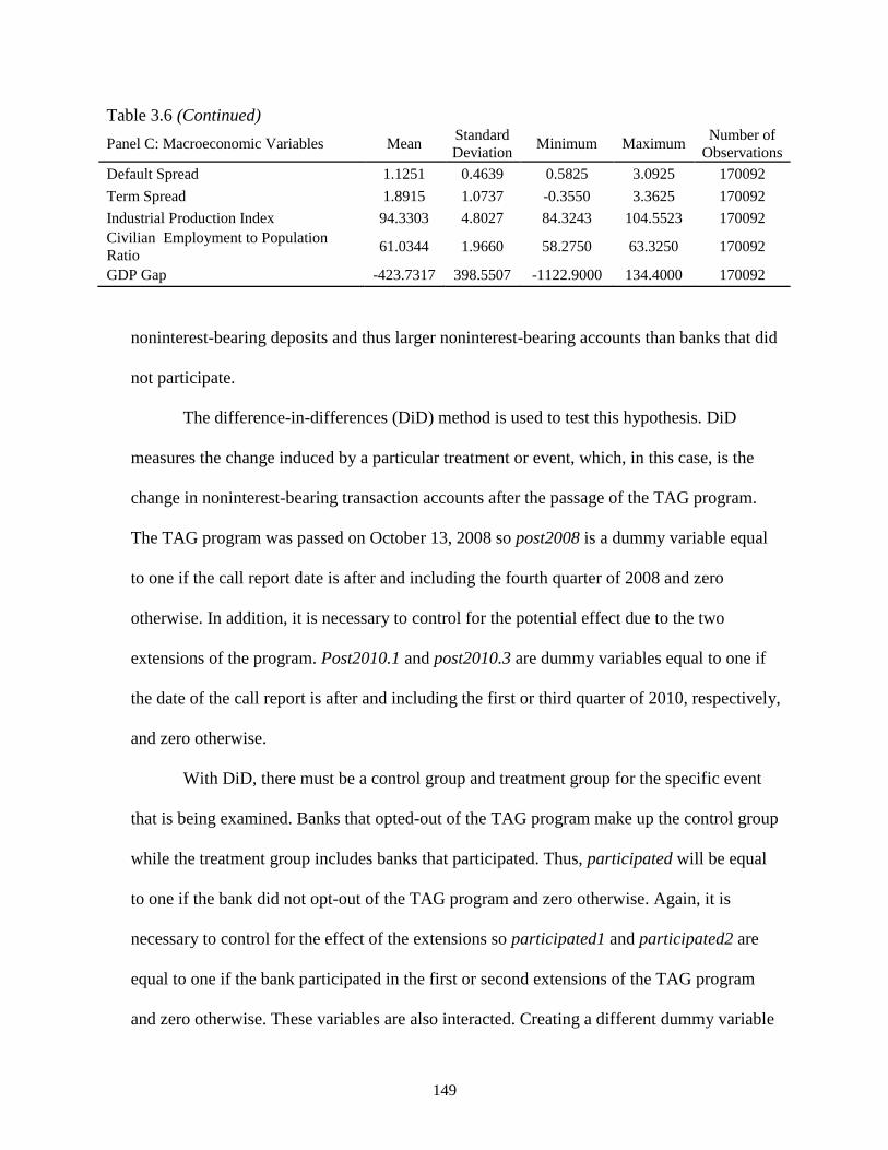
149


Panel C: Macroeconomic Variables Mean Standard


Number of

Observations

Default Spread 1.1251 0.4639 0.5825 3.0925 170092

Term Spread 1.8915 1.0737 -0.3550 3.3625 170092

Industrial Production Index 94.3303 4.8027 84.3243 104.5523 170092

Civilian Employment to Population

Ratio 61.0344 1.9660 58.2750 63.3250 170092

GDP Gap -423.7317 398.5507 -1122.9000 134.4000 170092

noninterest-bearing deposits and thus larger noninterest-bearing accounts than banks that did

not participate.

The difference-in-differences (DiD) method is used to test this hypothesis. DiD

measures the change induced by a particular treatment or event, which, in this case, is the

change in noninterest-bearing transaction accounts after the passage of the TAG program.

The TAG program was passed on October 13, 2008 so post2008 is a dummy variable equal

to one if the call report date is after and including the fourth quarter of 2008 and zero

otherwise. In addition, it is necessary to control for the potential effect due to the two

extensions of the program. Post2010.1 and post2010.3 are dummy variables equal to one if

the date of the call report is after and including the first or third quarter of 2010, respectively,

and zero otherwise.

With DiD, there must be a control group and treatment group for the specific event

that is being examined. Banks that opted-out of the TAG program make up the control group

while the treatment group includes banks that participated. Thus, participated will be equal

to one if the bank did not opt-out of the TAG program and zero otherwise. Again, it is

necessary to control for the effect of the extensions so participated1 and participated2 are

equal to one if the bank participated in the first or second extensions of the TAG program

and zero otherwise. These variables are also interacted. Creating a different dummy variable

150

for each period allows banks that opt-out during the extensions to switch in the middle of the

analysis, thus allowing me to separately examine the effect brought on by these institutions.

It is expected that for banks that did not opt-out of the TAG program and for dates

during which the unlimited insurance was offered that noninterest-bearing account balances

should have increased. The model is given by equation 1:

𝑛𝑜𝑛𝑖𝑛𝑡𝑒𝑟𝑒𝑠𝑡 𝑎𝑐𝑐𝑜𝑢𝑛𝑡𝑠𝑖𝑡 =

𝛼0 + 𝛽1𝑝𝑎𝑟𝑡𝑖𝑐𝑖𝑝𝑎𝑡𝑒𝑑 + 𝛽2𝑝𝑎𝑟𝑡𝑖𝑐𝑖𝑝𝑎𝑡𝑒𝑑1 + 𝛽3𝑝𝑎𝑟𝑡𝑖𝑐𝑖𝑝𝑎𝑡𝑒𝑑2 + 𝛽4𝑝𝑜𝑠𝑡2008 +

𝛽5𝑝𝑜𝑠𝑡2010.1 + 𝛽6𝑝𝑜𝑠𝑡2010.3 + 𝛽7(𝑝𝑎𝑟𝑡𝑖𝑐𝑖𝑝𝑎𝑡𝑒𝑑 ∗ 𝑝𝑜𝑠𝑡2008) + 𝛽8(𝑝𝑎𝑟𝑡𝑖𝑐𝑖𝑝𝑎𝑡𝑒𝑑1 ∗

𝑝𝑜𝑠𝑡2010.1) + 𝛽9(𝑝𝑎𝑟𝑡𝑖𝑐𝑖𝑝𝑎𝑡𝑒𝑑2 ∗ 𝑝𝑜𝑠𝑡2010.3) + 𝜀𝑖𝑡 (1)

where 𝑛𝑜𝑛𝑖𝑛𝑡𝑒𝑟𝑒𝑠𝑡 𝑎𝑐𝑐𝑜𝑢𝑛𝑡𝑠𝑖𝑡 is the amount of money in noninterest-bearing accounts

reported by bank i at time t and 𝜀 is the error term that varies across banks and quarters.

Standards errors are clustered by bank certificate number, which is an identification number

assigned to each bank by the FDIC. Because FINREG applied to every bank, observations

that occur past January 2011 are excluded. The data set consists of 312,530 bank-quarter

observations from January 2002 until December 2010.

The results from the estimation are shown in column 1 of Table 3.7. The point

estimates on the participation dummy variables show that firms participating during the

original program increased noninterest-bearing deposits, while banks that participated in the

second and third extension have fewer noninterest-bearing deposits. This result, however,

might be due to the large banks withdrawing from the program. There is an increase in

noninterest-bearing deposits across all periods of the unlimited insurance protection under

the TAG program (post2008, post2008.1, and post2008.3). Looking at the interactions

between the dates of the TAG program and bank participation, the results are similar to the

participation dummies in that banks that participated during the time of the TAG program

151

have more noninterest-bearing deposits during the TAG program, but the banks that

participated during the first and second extensions have fewer deposits during the periods of

unlimited insurance coverage. All variables and interactions are statistically significant at a

5% or 1% level. Thus, the large number of banks withdrawing from the first and second

extension of the TAG program seem to be affecting the results.

To test if the lower amounts of deposits held by banks during the first and second

extensions are due to large banks not participating in the program, I proceed by including an

addition dummy variable, largedummy, which equals one if the bank is classified as having

more than $10 billion in assets and zero otherwise. I also interact this variable with the other

variables from equation 1, creating a difference-in-difference-in-differences framework. In

addition, I control for the bank age by using the founding age, which is the date that the bank

started operations or the insured age which is the date that the bank became insured by the

FDIC. The need to control for firm age is that older, established banks might hold more

deposits simply due to size and not because of the TAG program.

These results are displayed in columns 2 through 4 of Table 3.7. The main point

estimates of interest are the three interactions with the participation dummies, dates, and

large dummy. In all three columns, large banks that participated during the original TAG

program have more noninterest-bearing deposits. This is statistically significant at a 1%

level. The large banks that participated during the first extension hold fewer deposits, a

finding that is statistically significant at a 5% level. Large banks that participated during the

second extensions also held fewer noninterest-bearing deposits, but the coefficient is not

statistically different than zero. Directing your attention to the interaction term between the

three participated dummies and time periods for the TAG program, banks that participated

152

Table 3.7 Difference-in-Differences This table shows the estimation using difference-in-differences analysis. The dependent variable is Noninterest-bearing accounts

held at FDIC insured banks. T-statistics are reported in parentheses where * is p<.10, ** is p<.05, and *** is p<.01.

(1) (2) (3) (4)

Participated 52439.4*** 65161.6*** 129365.5*** 146021.2***

(6.85) (7.41) (5.40) (4.99)

Participated1 -1150423.5*** -1198790.8** -1154515.8** -1125998.4**

(-2.59) (-2.45) (-2.42) (-2.39)

Participated2 -279633.5*** -236433.9*** -192880.6*** -174970.7**

(-3.86) (-3.14) (-2.61) (-2.41)

Post2008 16700.1*** 1025.6* -21942.0*** -17015.1***

(2.72) (1.83) (-3.45) (-3.31)

Post2010.1 813264.7** 156.3 -5503.8 -4270.8

(2.39) (0.03) (-0.96) (-0.77)

Post2010.3 236590.1*** 12161.0*** 8653.3** 9394.2**

(3.64) (2.96) (2.05) (2.25)

Large Dummy

-776597 -781360.3 -777476.9

(-0.46) (-0.47) (-0.46)

Participated*Post2008 56812.5*** 8263.5*** 8782.4*** 8686.6***

(3.83) (9.58) (9.81) (9.86)

Participated1*Post2010.1 -846977.1** 3157.6 3678.3 3533.1

(-2.39) (0.61) (0.70) (0.68)

Participated2*Post2010.3 -233603.9*** -10527.8** -9937.4** -10056.6**

(-3.43) (-2.45) (-2.31) (-2.34)

Participated*Large Dummy

-944260.8** -950605.7** -956722.6**

(-2.00) (-2.00) (-2.01)

Participated1*Large Dummy

1392842 1389887.9 1390622

(0.97) (0.97) (0.97)

Participated2*Large Dummy

-389965.9 -389334.2 -389416.1

(-0.53) (-0.53) (-0.53)

Post2008*Large Dummy

1024201.4** 1026963.9** 1025484.9**

(2.21) (2.21) (2.21)

Post2010.1*Large Dummy

10366058.9** 10364705.8** 10364346.5**

(2.41) (2.41) (2.41)

Post2010.3*Large Dummy

1495242.4*** 1494161.0*** 1493839.3***

(3.05) (3.04) (3.04)

Participated*Post2008*Large Dummy 3730341.5*** 3731162.5*** 3732920.8***

(3.40) (3.40) (3.40)

Participated1*Post2010.1*Large Dummy -12561062.6** -12558680.5** -12558243.6**

(-2.41) (-2.41) (-2.41)

Participated2*Post2010.3*Large Dummy -1159630.4 -1156975.5 -1156421.5

(-1.56) (-1.56) (-1.56)

Insurance Age

5885.6***

(3.67)

Founding Age

4633.0***

(3.57)

Constant 1434871.0*** 1439000.5*** 1037366.6*** 947292.6**

(3.20) (2.87) (2.59) (2.45)

N 312530 312530 312530 312530

R2 0.0113 0.0247 0.0234 0.0252

153

during the initial program held more noninterest-bearing deposits than firms that did not

participate. This result is statistically significant at a 1% level in all three columns. The

results for the first and second extensions suggest that even the smaller banks that exited the

program held more noninterest-bearing deposits than the smaller banks that participated. The

results remain even when controlling for founding age and insured age. The coefficients for

the age controls are both positive and statistically significant at a 1% level, suggesting that

older firms hold more noninterest-bearing accounts.

In conclusion, it is seen that during the initial periods of the TAG program banks that

participated held more noninterest-bearing accounts than firms that opted-out. This changes

during the second and third extensions when the banks that exited the program seems to hold

more noninterest-bearing accounts than the banks that participated, even when controlling for

the large banks that exited.

6.2 Structural Breaks in Noninterest-bearing Accounts and Corporate Cash Holdings

The second estimation is the Bai and Perron (2003) test for structural breaks. The Bai

and Perron analysis is a test for multiple endogenous structural breaks in time series data.

This test is used to determine if breaks in both noninterest-bearing accounts and cash

holdings occurred around similar times.

The Bai and Perron procedure allows one to choose the maximum number of breaks

to test as well as the minimum length of each break.85

A maximum of seven breaks is

allowed to occur because this would allow one break to occur at the start and end of each

period in which unlimited insurance is offered. Although a maximum of seven breaks are

85

In addition, they also allow either the constant and the lag of the variable of interest to break or just the constant.

In this paper, only the constant is allowed to break.

154

permitted to occur, there are occasions when the optimal number of breaks may be less than

seven. In order to select the optimal number of breaks, the Bayesian information criterion

(BIC) is used. A duration of at least two quarters is allowed for the break. Allowing a

duration of two quarters provides an opportunity to test if both extensions of the TAG

program had a significant effect on the series.

The predicted breaks for both noninterest-bearing accounts and cash holdings are

presented in Table 3.8. The first two panels list the predicted break dates for noninterest-

bearing accounts while the last two list the predicted break dates for cash holdings. In Panel

A, the BIC finds that the optimal number of break dates for the sum of noninterest-bearing

accounts is seven. The first six breaks are during the periods of unlimited insurance and the

final one is after the unlimited insurance expired. The F-statistic is 10.37, which is

statistically significant at a 1% level.86

The first two breaks occur around the TAG program;

the first break is two quarters prior to the program’s start and the second break is the quarter

before the second extension. The next four breaks occur during FINREG.

Panel B lists the predicted breaks for the ratio of noninterest-bearing deposits to total

deposits. The BIC finds that the optimal number of breaks is seven. The F-statistic is 11.31,

which is statistically significant at a 1% level. There are two breaks that occur prior to the

period of unlimited insurance. The next two breaks are during the TAG program and the next

two occur during FINREG. The final break occurs one year after FINREG stopped providing

full insurance protection.

The breaks in the sum of cash across firms is listed in Panel C. The BIC again finds

that seven breaks are optimal. The F-statistic is 20.73, which is significant at a 1% level. For

the corporate cash holdings series, a double break occurs in 2003 and a single break occurs in

86

The critical value for the 99th

percentile is 6.75 for seven breaks and one breaking parameter.

155

Table 3.8 Bai and Perron (2003) Predicted Breakpoints This table displays the results from the Bai and Perron (2003) test for structural breaks. The structural breaks for two measures of

noninterest-bearing deposits are presented first and then two measures for corporate holdings of cash are presented. The

maximum number of breaks was seven with a minimum duration of two quarters. Only the constant was allowed to break.

Panel A: Predicted Break Dates for Sum of Noninterest-Bearing Accounts

Predicted Breakpoint Lower 95% Upper 95% F(7) BIC(0) BIC(7)

2008:2 2007:4 2008:3 10.37 35.9 35.43

2010:2 2010:1 2011:2

2011:1 2010:4 2011:2

2011:4 2011:3 2012:1

2012:2 2012:1 2012:3

2012:4 2012:3 2013:1

2013:2 2013:1 2013:3

Panel B: Predicted Break Dates for Ratio of Noninterest-Bearing Accounts to Total Deposits


2005:4 2005:3 2006:1 11.31 -10.02 -10.55

2006:4 2006:3 2007:1

2008:2 2008:1 2008:3

2010:2 2010:1 2010:3

2011:1 2010:4 2011:2

2011:3 2011:1 2011:4

2014:1 2013:4 2014:3

Panel C: Predicted Break Dates for Sum of Cash


2003:1 2002:4 2003:2 20.73 20.61 20.28

2003:3 2003:2 2003:4

2007:1 2006:4 2007:2

2008:4 2008:3 2009:2

2009:2 2009:1 2009:3

2010:4 2010:3 2011:3

2013:1 2012:2 2013:2

Panel D: Predicted Break Dates for the Ratio of Cash to Total Assets


2002:4 2002:3 2003:1 10.25 -11.79 -12.29

2003:3 2003:2 2003:4

2005:4 2005:3 2006:1

2006:2 2005:2 2006:3

2008:4 2008:4 2009:1

2009:2 2009:1 2009:3

2009:4 2009:2 2010:1

156

2007. During this time, banks within holding companies began to allocate deposits in

amounts less than $100,000 in order to circumvent the FDIC’s $100,000 limit, yet still

achieve full insurance (Pennacchi (2006)). The next three breaks occur during the unlimited

insurance period. The first is during the fourth quarter of 2008. This is during the quarter in

which the TAG program was passed. The next break is during the second quarter of 2009

when the FDIC was considering the first extension of the TAG program. The following break

is in the fourth quarter of 2010, which is the final quarter of the TAG program protection and

the quarter before FINREG took effect. The final break is during the first quarter of 2013,

which is one quarter after the unlimited insurance protection provided by FINREG expired.

The final measure, the ratio of cash and cash equivalents to total assets, is presented

in Panel D. The BIC finds that seven breaks is the optimal number of breaks. The F-statistic

is 10.25, which is significant at a 1% level. Four breaks are seen during the early and mid-

2000’s. There are three breaks found during the unlimited insurance periods. The first during

the fourth quarter of 2008 was during the first quarter of the passage of the TAG program.

The second break during the second quarter of 2009 is prior to the announcement of the first

extension of the TAG program, but continues through the extension. The final break is during

the fourth quarter of 2009, prior to the extensions. It is interesting to note that with both

measures of cash there is a break during the fourth quarter of 2008. While this is the quarter

that noninterest-bearing deposits were fully insured, it is also during the financial crisis and

the quarter that the National Bureau of Economic Research made an announcement that the

economy was in a recession. This is interpreted as further evidence that there is a need to

control for the business cycles when looking at the effect on cash.

157

In summary, although a direct relationship between increases in cash held by

corporations and noninterest-bearing accounts cannot be made, evidence is provided that

both increased during the periods of unlimited insurance.

6.3 Regression Analysis

How did cash holdings change during the periods of unlimited insurance? If

corporations are holding more cash due to the unlimited insurance, cash holdings should

increase and thus a positive relationship should be seen during the dates. To test this,

multiple models are used: an ordinary least squared (OLS), a fractional QMLE probit and a

random effect double censored Tobit model. The OLS regression is the typical regression

model used in the cash holdings literature. This regression has several shortcomings. The

dependent variable in all regressions is cash holdings and represents a fractional value,

between and including zero and one. Thus, the data is naturally constrained to lie within

these values. The OLS model does not place restrictions on the predicted values of the model

and thus the predicted values can lie outside of this range. The second restriction is that it

does not allow one to test for the effects of a lagged dependent variable. Thus, by not

restricting the predicted values and not allowing a lagged dependent variable it might bias the

results. The second model, the fractional probit, is similar to the model used by Wooldridge

and Papke (2006). This model allows for the test of a naturally restricted dependent variable.

However, it would be nice to control for the unobserved heterogeneity and a lagged

dependent variable. This model does not allow one to control for both in the same regression.

The final model used is the random effect Tobit model with double censoring at zero and

one. This model is similar to that used in Loudermilk (2007). The double censored Tobit

158

model makes it possible to control for a constrained dependent variable while also

controlling for unobserved heterogeneity and a lagged dependent variable.

The lag of cash holdings for the prior quarter is included in the fractional probit

model and the double censored Tobit model because quarterly data is being used and past

quarterly cash holdings are likely to influence cash holdings in future quarters. Even though

the model does support values at the corners, two dummy variables are included to control

for these corner values: a dummy variables that is equal to one if the lag of cash holdings is

equal to one and zero otherwise and a dummy variable that is equal to one if the lag is equal

to zero and zero otherwise.a Year and industry dummies are also included in all regressions

and standard errors are clustered at a company level. As discussed, the increased insurance

did occur over the time of the Great Recession and cash holdings have been shown in prior

literature to vary during business cycles. To control for recessions, the five additional

macroeconomic variables are also included.

Table 3.9 displays the results from all three models including the dates of the TAG

program, first and second extension of the TAG program, and FINREG as well as including

the macroeconomic variables. Column 1 reports the results from an OLS regression. None of

the unlimited insurance dummies are statistically significant at conventional levels. When

looking at the macroeconomic variables, the term spread and civilian employment to

population ratio are both statistically significant and of the predicted sign. The other three

macroeconomic variables are not statistically different from zero. This could be because

there is a high correlation between some of the macroeconomic indicators. These results

suggest the reason that firms increased cash holdings during this time is due to recessionary

reasons rather than unlimited insurance on bank accounts in the later periods.

a The coefficients on the corner control dummies are not included but are available upon request.

159

Table 3.9 Regression Analysis for Cash Holdings This table displays the results for the regression anaylsis over the time frame of 2002-2013. The dependent variable in all

regressions is cash holdings. The rest of the variables are as described in Table 3.6. T-statistics are reported in parentheses where

* is p<.10, ** is p<.05, and *** is p<.01.

(1) (2) (3) (4)

OLS Fractional Probit Fractional Probit Double-Censored

Tobit

TAGP Dummy -0.00057 -0.0382** -0.00461 -0.00484

(-0.18) (-2.20) (-0.26) (-1.58)

Extension TAGP Dummy 0.00528 0.0227 0.0269 0.00545

(1.24) (1.12) (1.14) (1.62)

Second Extension TAGP Dummy 0.00532 0.0282 0.0204 0.0063**

(1.36) (1.64) (0.98) (2.16)

FINREG Dummy -0.00042 0.0109 -0.0104 0.00311

(-0.15) (0.88) (-0.70) (1.46)

Default Spread 0.00035 0.00923 0.00054 0.00148

(0.23) (1.30) (0.06) (1.16)

Term Spread 0.0049*** 0.0113*** 0.0199*** 0.0027***

(5.27) (2.61) (4.28) (3.62)

Industrial Production Index 0.00042 0.0044*** 0.00126 0.00088***

(1.29) (2.76) (0.64) (3.30)

Civilian Employment to Population Ratio -0.0037** -0.0227*** -0.0221** -0.0025*

(-2.40) (-2.89) (-2.25) (-1.87)

GDP Gap 0.00001 -0.00009*** 0.00005* -0.00001***

(1.36) (-4.08) (1.79) (-3.28)

Market to Book 0.003*** 0.0037*** 0.0091*** 0.0007***

(7.86) (6.00) (6.74) (9.64)

Cash Flow 0.00861 0.0298* 0.0579* 0.0045**

(1.00) (1.74) (1.81) (2.36)

Net Working Capital-to-Assets -0.00397 -0.0446*** -0.0163 -0.0052***

(-1.55) (-9.46) (-1.47) (-9.62)

Capital Expenditure-to-Assets -0.116*** -0.875*** -1.025*** -0.217***

(-3.10) (-7.62) (-3.65) (-17.76)

Leverage -0.047*** -0.108*** -0.166*** -0.0133***

(-11.20) (-14.59) (-9.06) (-16.86)

R&D to Sales 0.004*** 0.00093 0.0083*** 0.0006***

(5.50) (1.24) (3.82) (4.86)

Acquisitions-to-Assets -0.169*** -2.139*** -1.218*** -0.351***

(-14.40) (-31.01) (-10.54) (-37.67)

Dividend Dummy 0.00326 -0.0207*** 0.0362*** -0.0017*

(1.58) (-3.36) (2.83) (-1.87)

Investment Grade Dummy 0.00142 -0.00552 -0.00458 0.0011

(0.41) (-0.57) (-0.17) (0.68)

Size -0.022*** -0.0047*** -0.108*** -0.0092***

(-13.71) (-3.82) (-10.22) (-21.96)

Cash Flow Riskiness -0.00007 -0.0008* -0.00058 -0.00006

(-0.32) (-1.94) (-0.58) (-0.97)

Lagged Cash Holdings

3.157***

0.756***

(194.96)

(415.21)

Constant 0.326*** -0.794* 0.163 -0.102

(3.39) (-1.80) (0.02) (-0.39)

160


N 164771 160712 164771 153481

Industry and Year Dummies Yes Yes Yes Yes

Mundlak-Chamberlain Devices No No Yes Yes

Corner Dummies No Yes No Yes

Log Likelihood Ratio - -37847.2 -47795.3 183366.2

R2 0.229 - - -

In columns 2 and 3 the results from the fractional probit model are presented. Since I

cannot control for a lagged value of the dependent variable and unobserved heterogeneity,

the results in column 2 are from the model controlling for cash holdings from the previous

quarter while the results in column 3 are from the model where I control for unobserved

heterogeneity. The TAGP dummy has a negative and statistically significant relationship with

cash holdings at a 5% level. The relationship suggests that cash holdings declined during the

initial time frame of the TAG program from the fourth quarter of 2008 until the fourth

quarter of 2009. The other three dummy variables for unlimited insurance are not statistically

different from zero. In column 3, none of the unlimited insurance dummy variables are

statistically different from zero, suggesting that the business cycle is explaining the variation

in cash holdings and not the unlimited insurance periods.

Column 4 presents the results from the random effects double censored Tobit model.

When looking at the unlimited insurance dummies there is not much of an effect seen except

for the second extension TAGP dummy, which is positive and statistically significant at a 5%

level.

In summary, after controlling for common macroeconomic variables that change

during recessions, companies appear to have not increased cash holdings due to the unlimited

insurance Acts but due to the ongoing recession.

161

7. Conclusion

This paper examines the periods of unlimited FDIC insurance guarantees provided by

the Transaction Account Guarantee Program and the Dodd-Frank Wall Street Reform and

Consumer Protection Act and the effect that this may have had on corporate cash holdings.

After an extensive review of the Acts, I show that noninterest-bearing accounts increased

during periods of unlimited insurance and further document that this increase was not driven

by withdrawals from interest-bearing accounts. Using Flow of Funds data, I then show that a

large increase in cash holdings held in checking deposits also took place during this time

period.

This paper then uses both time series and panel regression techniques to examine the

increase in noninterest-bearing deposits and cash holdings. First, difference-in-differences

and difference-in-difference-in-differences analysis is used to show that an increase in

noninterest-bearing deposits took place at banks that participated during the original periods

of the TAG program from October 2008 until December 2009. It is further shown that firms

that opted-out of the first and second extensions held more noninterest-bearing deposits than

banks that participated, even when controlling for the large banks that exited the program.

Using Bai and Perron (2003) structural break analysis, several structural breaks in

noninterest-bearing accounts and cash holdings are found around similar times as the periods

of unlimited insurance, demonstrating that not just noninterest-bearing deposits increased,

but also cash holdings. Finally, I use ordinary least squares, fractional probit, and double-

censored Tobit models and show that after controlling for the most recent financial crisis, the

increase in cash holdings is less prominent during the periods of unlimited insurance. This

finding suggests that the increase in cash holdings was due to the recession and not

162

necessarily the unlimited insurance, even though the fully insured deposits might have

presented a good place to store the increase in cash balances.

163

References

2011 Association for Financial Professionals Liquidity Survey.

http://www.afponline.org/liquidity/ (accessed April 16, 2014).

2012 Association for Financial Professionals Liquidity Survey.

http://www.afponline.org/liquidity/ (accessed April 16, 2014).

Almeida, H., M. Campello, and M. S. Weisbach, 2004, The cash flow sensitivity of cash,

Journal of Finance, 59, 1777-1804.

Azar, J., J. Kagy, and M. C. Schmalz, 2014, Can changes in the cost of capital resolve the

corporate cash puzzle?, unpublished working paper.

Bai, J. and P. Perron, 2003, Computation and analysis of multiple structural change models,

Journal of Applied Econometrics 18, 1-22.

Bates, T. W., K. M. Kahle, and R. M. Stulz, 2009, Why do U.S. firms hold so much more cash

than they used to?, Journal of Finance 64, 1985-2021.

Baum, C. F., M. Caglayan, N. Ozkan, and O. Talavera, 2006, The impact of macroeconomic

uncertainty on non-financial firms’ demand for liquidity, Review of Financial Economics

15, 289-304.

Campello, M., J. R. Graham, and C. R. Harvey, 2010, The real effects of financial constraints:

Evidence from a financial crisis, Journal of Financial Economics 97, 470-487.

Chen, N.-F., 1991, Financial investment opportunities and the macroeconomy, Journal of

Finance 46, 1467-1484.

Christensen, J., J. Lopez, and G. Rudebusch, 2009, Do central bank liquidity facilities affect

lending rates? Working paper, Federal Reserve Bank of San Francisco.

Duchin, R., O. Ozbas, and B. A. Sensoy, 2010, Costly external finance, corporate investment,

and the subprime mortgage credit crisis, Journal of Financial Economics 97, 418-435.

Duygan-Bump, B., P. Parkinson, E. Rosengren, G. A. Suarez, and P. Willen, forthcoming, How

effective were the Federal emergency liquidity facilities? Evidence from the Asset

Backed Commercial Paper Money Market Mutual Fund Liquidity Facility, Journal of

Finance.

164

Fama, E. and K. French, 1989, Business conditions and expected returns on stocks and bonds,


Federal Deposit Insurance Corporation, 2010, Quarterly Banking Profile, FDIC Quarterly 4, 1-

28.

Federal Deposit Insurance Corporation, 2013, Quarterly Banking Profile, FDIC Quarterly 7, 1-

26.

Ferreira, Miguel A., Custodio, Claudia and Raposo, Clara C., Cash Holdings and Business

Conditions (February 2005). http://ssrn.com/abstract=608664

Hoskins, S. M., 2012, An overview of the Transactions Account Guarantee (TAG) program and

the potential impact of its expiration of extension, Congressional Research Service,

R42787.

Kelly, S. “Response Tepid as Reg Q Repeal Nears.” TreasuryandRisk.com, July 21, 2011.

http://www.treasuryandrisk.com/2011/07/12/response-tepid-as-reg-q-repeal-nears

(accessed September 19, 2012)

Kuritzkes, A., T. Schuermann, and S. M. Weiner, 2005, Deposit insurance and risk management

of the U.S. banking system: What is the loss distribution faced by the FDIC? Journal of

Financial Services Research 27, 217-242.

Loudermilk, M. S., 2007, Estimation of fractional dependent variables in dynamic panel data

models with an application to firm dividend policy, Journal of Business & Economic

Statistics, 25, 462-472.

Marcus, A. J. and I. Shaked, 1984, The valuation of FDIC deposit insurance using option-pricing

estimates, Journal of Money, Credit and Banking, 16, 446-460.

Merton, R. C., 1977, An analytic derivation of the cost of deposit insurance and loan guarantees,

Journal of Banking and Finance 1, 3-111.

National Bureau of Economic Research (NBER) US Business Cycle Expansions and

Contractions, http://www.nber.org/cycles.html (accessed August 17, 2011).

Opler, T., L. Pinkowitz, R. Stulz, and R. Williamson, 1999, The determinants and implications of

corporate cash holdings, Journal of Financial Economics 52, 3-46.

Pennacchi, G., 2006, Deposit insurance, bank regulation, and financial system risks, Journal of

Monetary Economics 53, 1-30.

Pozar, Z., 2011, Institutional cash pools and the Triffin Dilemma of the U.S. banking system,

IMF Working Paper, 1-35.

165

Regions Financial Corporation, 2009 Annual Report,

http://files.shareholder.com/downloads/AMDA-

J4ZTD/2342666796x0x510710/CE354529-C3C7-4DFC-AEE4-

A7E6174A4AD8/2009AR.pdf (accessed April 26, 2013).

Regions Financial Corporation, 2011 Annual Report,

http://files.shareholder.com/downloads/AMDA-

J4ZTD/2342666796x0x549181/D137F486-A274-4734-A909-

D2E043B6DF42/2011_Annual_Report_with_10-K_FINAL_3.5.12___REGIONS.pdf

(accessed April 26, 2013).

Schich, A., 2008, Financial crisis: Deposit insurance and related financial safety net aspects,

Financial Market Trends 2, 1-39.

Stone, A. L. and B. Gup, 2012, Do business cycles influence corporate cash holdings?, Working

paper.

Stroebel, J. C. and J.B. Taylor, 2009, Estimated impact of the Fed’s mortgage-backed securities

purchase program, NBER Working paper 15626.

Wheelock, D. C. and M. E. Wohar, Can the term spread predict output growth and recessions? A

survey of the literature, Federal Reserve Bank of St. Louis Review 91, 419-440.

Wu, T., 2011, The U.S. money market and the Term Auction Facility in the financial crisis of

2007-2009, Review of Economics and Statistics 93, 617-631.

166

Appendix

Table A.3.1 List of Corporate Determinant Variables and Definitions

Variables Definition

Cash Holdings Cash and Cash Equivalents divided by Total Assets

Market-to-Book Market Value per Share to the stated Book Value of Equity

Cash Flow Earnings after Interest, Taxes, and Dividends, but before

Depreciation, divided by Total Assets

Net Working Capital Net Working Capital minus Cash and Marketable Securities divided

by Total Assets

Capital Expenditure-to-Assets Capital Expenditure divided by Total Assets

Leverage Long Term Debt plus Current Debt divided by Total Assets

R&D to Sales Research and Development Expense divided by Sales

Acquisitions-to-Assets Acquisitions divided by Total Assets

Dividend Dummy Indicator variable equal to one if the company pays a common

dividend and zero otherwise

Investment Grade Dummy Indicator variable equal to one if a company has an investment grade

bond or commercial paper rating, otherwise the dummy equals zero

Size Natural log of a firm’s Total Assets in 2009 dollars

Cash Flow Riskiness

The standard deviation of industry cash flows calculated as the

standard deviation of cash flows for the previous twenty years, if

available. I do require that firms have at least five years of data to

calculate cash flow riskiness. Observations are then averaged across

the two-digit SIC code.

TAGP Dummy

Dummy variable that equals one if the date of the quarterly report

covers the original dates of the TAGP from October 14, 2008 until

December 31, 2009 and zero otherwise

Extension TAGP Dummy


covers the original dates of the first extension of the TAGP from

January 1, 2010 until June 30, 2010 and zero otherwise

Second Extension TAGP Dummy


falls within the time frame of the second extension of the TAGP from

July 1, 2010 until December 31, 2010 and zero otherwise

FINREG Dummy Dummy variable that equals one if the quarterly report date falls

within January 1, 2011 and December 31, 2012 and zero otherwise

167

Figure A.3.1 Liquid Assets Held by Nonfinancial Businesses This figure presents data on the amount of liquid assets held by all nonfinancial businesses from January 2002 until September

2014. Data is obtained from the Flow of Funds account L.101. The Other category is the sum of security repurchase agreements,

credit market instruments, commercial paper, treasury securities, agency-and GSE- backed securities, and municipal securities

and loans. The shaded region is from 2008 until 2012. The bars separate the time periods of the Temporary Account Guarantee

(TAG) Program, the first and second extension to the TAG program and the Dodd-Frank Wall Street Reform and Consumer

Protection Act (FINREG).

168

Figure A.3.2 Interpolated Cash and Cash Equivalents and Quarterly Cash and Cash Equivalents This figure presents data on the measure of quarterly cash and cash equivalents to the interpolated measure of cash and cash

equivalents from January 2002 until September 2014. Data is collected from Compustat Quarterly files for the quarterly measure

of cash and Compustat Annual files for the annual measure of cash that is interpolated to quarterly data. The shaded region is

from October 2008 until December 2012. The bars separate the time periods of the Temporary Account Guarantee (TAG)

Program, the first and second extension to the TAG program and the Dodd-Frank Wall Street Reform and Consumer Protection

Act (FINREG).

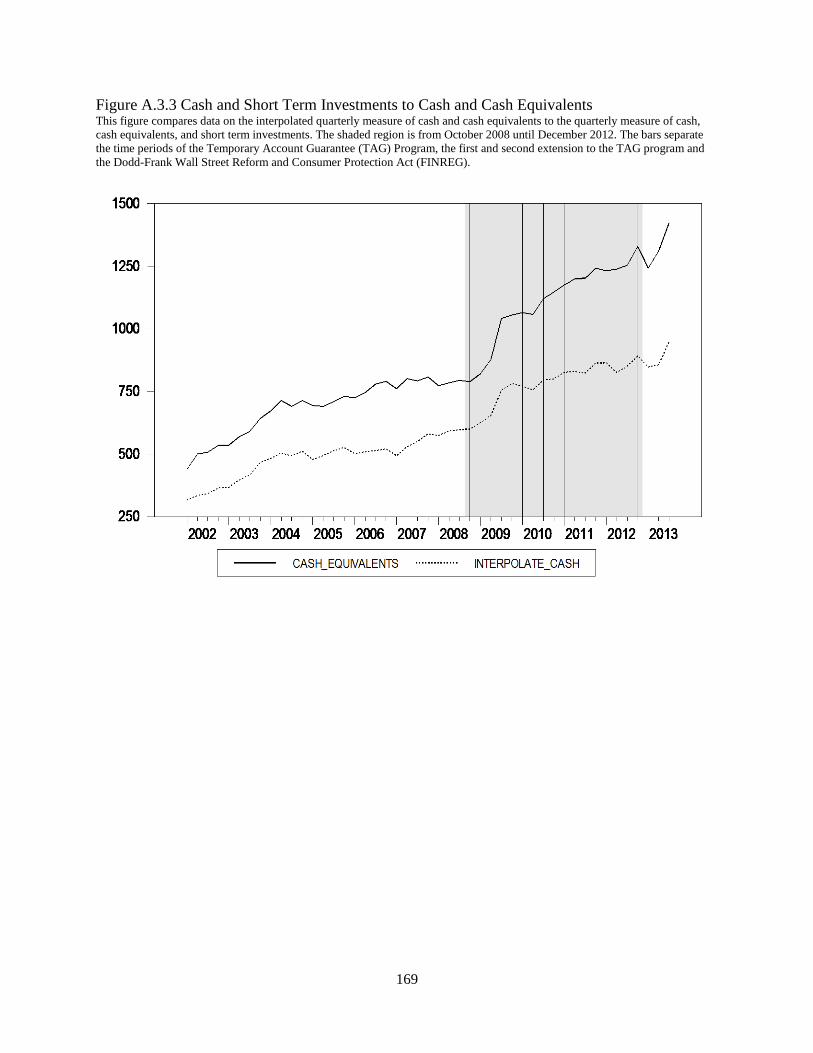
169

Figure A.3.3 Cash and Short Term Investments to Cash and Cash Equivalents This figure compares data on the interpolated quarterly measure of cash and cash equivalents to the quarterly measure of cash,

cash equivalents, and short term investments. The shaded region is from October 2008 until December 2012. The bars separate

the time periods of the Temporary Account Guarantee (TAG) Program, the first and second extension to the TAG program and

the Dodd-Frank Wall Street Reform and Consumer Protection Act (FINREG).

170

CONCLUSION

The conclusions reached in this dissertation have important implications for the literature

on corporate cash holdings, specifically the external determinants that drive firms to hold cash

reserves. The first essay shows that despite early economy theories that showed cash holdings

will vary inversely with interest rates, firms with below mean levels of corporate cash holding do

not vary inversely. The second essay shows that corporations may react more to the

announcement of recessions as made by the National Bureau of Economic Research than

previously thought. It is found that corporations increase their holdings of cash the quarter an

announcement is made that the economy is in a recession. In the third essay, the periods of

unlimited FDIC insurance guarantees for noninterest-bearing accounts provided by the

Transaction Account Guarantee Program and Section 343 of the Dodd-Frank Wall Street Reform

and Consumer Protection Act is examined. It is found that corporations did not hold cash

because of the unlimited levels of insurance, but held additional cash reserves because of the

ongoing recession.

three essays on the determinants of corporate cash...

Documents