three essays on the effects of budgetary policy in
TRANSCRIPT

HAL Id: tel-00606175https://tel.archives-ouvertes.fr/tel-00606175v2
Submitted on 16 Sep 2014
HAL is a multi-disciplinary open accessarchive for the deposit and dissemination of sci-entific research documents, whether they are pub-lished or not. The documents may come fromteaching and research institutions in France orabroad, or from public or private research centers.
L’archive ouverte pluridisciplinaire HAL, estdestinée au dépôt et à la diffusion de documentsscientifiques de niveau recherche, publiés ou non,émanant des établissements d’enseignement et derecherche français ou étrangers, des laboratoirespublics ou privés.
Three essays on the effects of budgetary policy indeveloping countriesMouhamadou Moustapha Ly
To cite this version:Mouhamadou Moustapha Ly. Three essays on the effects of budgetary policy in developing coun-tries. Economics and Finance. Université d’Auvergne - Clermont-Ferrand I, 2011. English. �NNT :2011CLF10358�. �tel-00606175v2�

1
Université d‟Auvergne Clermont-Ferrand I
Faculté de Sciences Economiques et de Gestion
Centre d‟Etudes et de Recherches sur le Développement International (CERDI)
Trois essais sur les Effets de la Politique Budgétaire dans les Pays en
Développement
Thèse nouveau Régime Présenté et soutenue publiquement le 20 Juin 2011
Pour l‟obtention du titre de Docteur ès Sciences Economiques
Par
Mouhamadou Moustapha LY
Sous la direction de Mr. Jean-Louis Combes, Professeur
Mr. Adama Diaw, Professeur
Membres du Jury :
Gilbert Colletaz, Professeur Université d‟Orléans (Laboratoire d‟Economie d‟Orléans)
Marc-Alexandre Sénégas, Professeur Université Montesquieu-Bordeaux IV
Xavier Debrun, Deputy Division Chief, IMF Fiscal Department
Alexandru Minea, Professeur Université d‟Auvergne (CERDI)
Jean-Louis Combes, Professeur Université d‟Auvergne (CERDI)
Adama Diaw, Professeur Université Gaston Berger de Saint-Louis du Sénégal
2
L’Université d’Auvergne Clermont-1 n’entend donner aucune approbation ni
improbation aux opinions émises dans la thèse. Ces opinions doivent être
considérées comme propres à l’auteur.

3
REMERCIEMENTS
J‟adresse mes remerciements les plus profonds à l‟ensemble du personnel de recherche et
administratif du CERDI pour avoir rendu ce long séjour à l‟Université d‟Auvergne des
plus agréables.
Je remercie profondément le Professeur Adama Diaw pour avoir accepté de co-diriger
cette thèse. Son implication dans ce travail, ses conseils ainsi que sa constante sollicitude,
auront été indispensables à la bonne réalisation de cette thèse. Ses grandes qualités
humaines m‟auront marquées.
Ma profonde gratitude aux professeurs Gilbert Colletaz, Alexandru Minea et Marc-
Alexandre Sénégas ainsi qu‟à Xavier Debrun pour avoir accepté de faire partie du jury de
thèse.
Je remercie le Ministère français des affaires étrangères à travers son Service de
Coopération et d‟Action Culturel de l‟ambassade de France à Dakar pour avoir appuyé
cette thèse.
A l‟ensemble des collègues doctorants et promotionnaires de magistère au Cerdi je dis
merci pour ces belles années de profonde amitié et de franche fraternité. Souvent en votre
compagnie, l‟espace convivial des chambres universitaires de Clermont-Ferrand a été le
lieu de débats passionnés sur l‟Afrique et son développement. Je profite de cette occasion
pour nous rappeler la promesse qu‟on a souvent faite à notre chère Afrique : celle de la
servir en tout lieu et en tout temps. Merci à Mme Matilda Ndow pour avoir pris le temps
de relire intégralement et avec beaucoup d‟attention cette thèse.
A l‟ensemble de mes amis et de la communauté sénégalaise à Clermont-Ferrand je dis
merci. A mes amis Ndiogou Malick Fall et Cheikh Mbacké Seck fidèles parmi les fidèles.
Et enfin et comme on le dit souvent : le meilleur pour la fin. Qu‟il me soit permis de
rendre un hommage particulier au Pr Jean-Louis Combes. Depuis maintenant une
décennie Mr Combes a été d‟un soutien sans faille et portant un intérêt particulier à mes
travaux depuis mon Master Recherche et bien avant encore. A travers ces années il m‟a
été donné d‟apprécier sa grande rigueur scientifique ainsi que ses qualités humaines si
rares. Ses conseils avisés auront été déterminants à la réflexion ainsi qu‟à la rédaction de
cette thèse. A toutes les étapes de cette thèse et à chaque fois où j‟ai fait face au doute et à
la difficulté Jean-Louis Combes, sans se lasser une seule fois, a su non seulement trouver
les bons mots mais aussi le soutien adéquat pour me permettre de continuer le combat.
J‟associe également son épouse Madame le Professeur Pascal Motel Combes aux mêmes
remerciements.

4
Une profonde reconnaissance pour Serigne Babacar ibn Abdoul Aziz Sy Dabakh et
Thierno Habib ibn Thierno Mountaga Ahmed Mountaga Tall deux branches d‟un même
arbre qu‟est la Tidjaniya. Vos deux ancêtres auront marqué l‟histoire de notre chère
Sénégal. Avec Thierno Habib Tall je ne compte plus le temps passé au téléphone à me
prodiguer des conseils et à m‟apporter un réconfort permanent. Serigne Mbaye Sy Abdou
comme on l‟appelle affectueusement est toujours d‟une oreille très attentive et malgré ses
charges administratives importantes est d‟un appui affectueux et spirituel indéfectible.
Plus haut je parlais d‟un arbre fruitier dont Cheikh Ahmed Tidjani est la racine profonde
et irrigatrice, El Hajj Omar Tall et El Hajj Malick en constituent le solide tronc. Quant à
ceux qui voudraient goutter aux fruits de cet arbre, fruits sucrés au parfum enivrant de
bonheur il leur faudra aller les cueillir à Tivaouane.
A ma famille à qui je dois tout. A mes nièces Fatou Kane, Safiétou Yeya Kane et Mbarka
Ndiaye que j‟aime d‟un amour qui tire des larmes. A mes neveux Mamadou Racine Kane,
Mamadou Alpha Kane et Balla Ndiaye. A vous la jeune génération montante de la famille
je formule des prières pour que le TOUT PUISSANT vous accorde une longue vie ainsi
qu‟une réussite totale dans tout ce que vous entreprendrez dans votre vie. A mes sœurs
Yeya, Sala, Coumba et Mariam je dis merci pour votre soutien indéfectible toutes ces
années ainsi que pour la tendresse avec laquelle vous m‟entourez. Je remercie
profondément mon frère ainé Alpha Amadou Ly qui veillait continuellement sur moi
quand j‟étais encore enfant et qui continue à le faire maintenant, sur mon épaule tu
trouveras toujours un appui et un réconfort. A mes frères Mamadou Kane, Ibrahima
Kane et Ibrahima Ndiaye.
A ma douce moitié Loubna pour son affection... Merci pour ta grande patience pendant
toutes ces années. La rédaction d‟une thèse est un exercice parfois très prenant et je sais
que mes absences répétées et les longues nuits devant l‟ordi n‟auront pas toujours été
faciles. Pendant tous ce temps tu as continué à me pousser et à m‟encourager. Tes
commentaires et critiques auront bien souvent permis d‟améliorer et de préciser
davantage mes idées. Ton amour et ton soutien m‟auront permis dépasser bien
d‟obstacles. A ma belle famille j‟exprime ma profonde gratitude pour leur accueil toujours
chaleureux et leur convivialité sans cesse renouvelée.
Et pour finir je dédie cette thèse à mes parents. Trouver les mots pour exprimer mes
sentiments à leur égard est très difficile voire impossible. Mon père a eu deux passions
dans sa vie : la cause éducative au Sénégal et sa famille. Ma mère qui nous a toujours
enveloppés d‟un manteau d‟amour très épais et nous a beaucoup protégé et continue à la
faire. Les mots me manquent. Puisse le TOUT PUISSANT vous récompenser
généreusement et vous garder longtemps parmi nous.

5
A Grand-père Ali Bocar Kane
A Mamadou Lamine Ly dernier Almamy du Fouta
A El Hajj Saïdou Nourou Tall & El Hajj Abdoul Aziz Sy Dabakh : toujours dans nos mémoires.

6
TABLE OF CONTENTS
CHAPTER 1: GENERAL INTRODUCTION & OVERVIEW ......................................... 7
CHAPTER 2: FISCAL POLICY SHOCKS IN DEVELOPING COUNTRIES: A PANEL
STRUCTURAL VAR APPROACH .................................................................................... 39
CHAPTER 3: IMPACT OF LARGE FISCAL IMBALANCE IN ADVANCED
COUNTRIES ON DEVELOPING COUNTRIES........................................................... 85
CHAPTER 4: FISCAL POLICY FOR STABILIZATION IN DEVELOPING
COUNTRIES: A COMPARATIVE APPROACH ........................................................... 145
GENERAL CONCLUSION ............................................................................................ 208
REFERENCES ................................................................................................................ 213
Chap1 : General Introduction & Overview
7
Chapter 1: General
Introduction & Overview

Chap1 : General Introduction & Overview
8
1.1 Introduction
Fiscal policy along side with monetary policy is one of the main tools available to
public authorities to intervene and influence the real economy. The recent financial crisis
(started in 2008) has shown the importance of government intervention to stabilize and
alleviate any threat on the economy. Indeed fiscal activism, after more than two decades
of neo-classical and the “no fiscal dominance” paradigm, has come back on the top of
government agendas in recent years. In both developing and advanced economies, IMF
has called for fiscal stimulus combined with easing monetary policies in response to the
global downturn. In a Staff Policy Notes (IMF, 2009), the IMF research department from
a multi-country structural model finds that with the right policies, both emerging and
advanced countries could support aggregate demand and restore economic growth. Such
worldwide fiscal stimulus policy is believed to end the global crisis through the large
multiplicative effects1. However the come-back of Keynesian ideas poses some challenges
on which I will be back later in this section. Despite the renewal of interest on fiscal
policy, its effects on economic activity still remain not well known.
As it is usually defined fiscal policy is the use of public spending and taxes to influence
economic activity toward more expansion or contraction depending on the situation. All
along history of economics, views and theories on the efficiency of fiscal policies have
been most of the time contradictory.
The recourse to public finances as a tool to influence economic activity formally started
during the great depression in 1929. Before that date, the budget had no economic role it
was only dedicated to current spending of the central administration. Indeed during
1930s‟ depression some governments have started considering the budget as an economic
policy tool. The analysis from the British economist John Maynard Keynes has given a
theoretical foundation for such policies, showing that public spending and tax revenues
1 In the same note, for countries with financing constraints (highly indebted countries or low fiscal
resource endowed countries) the IMF has advised at least to keep unchanged public expenditures
especially social ones.

Chap1 : General Introduction & Overview
9
are efficient tool to regulate economic cycles. In 1929 the recession was very severe, for
instance in 1933 one American worker in every four was unemployed. Additional to that
25% unemployment rate, 20% of New York City school children were under weight and
malnourished. In this context public intervention was quasi-compulsory and necessary.
The US government announced a wide economic plan, the New Deal, to address these
issues. In the first years the plan was concerned with relief (food and shelter for millions
of indigents and unemployed). Then the policy shifted toward recovery (creation of state
agencies such as National Recovery Act in 1933, and National Industrial Recovery Act).
Several arguments have been advanced to justify the use of fiscal policy as an economic
policy tool. The first of these arguments has been the direct Keynesians ideas and their
extensions.
J. M. Keynes, in his General Theory (1935), has identified two channels through which
government budget could be considered as an economic policy tool. The first role for
fiscal authorities is to ensure a better distribution of income. Greater income equality puts
more money into hand of people with higher marginal propensity to consume (MPC)
leading to increased consumption (Pressman, 1997). The second aspect of this theory
argues that public spending was the principal mean available to protect the economy
against fluctuations through the multiplicative effect. During the great depression and
even after, the two Keynesian principles guided major public policies in the developed
world and in new countries as well. For instance in the UK public spending jumped from
25% of GNP during pre-war period to more than 50% during mid-1970s. On the same
vein, developing countries‟ public finances have also been characterized by high level of
spending (weak fiscal revenues) and deficits since 1960s but unfortunately the expected
results have not been always obtained.
On straight line with traditional Keynesian ideas, other authors developed arguments that
are related to the important short-term social waste associated to business cycles. For
such authors (e.g. Galí, 2005) business cycles induces important costs in terms of

Chap1 : General Introduction & Overview
10
economic efficiency2 and output volatility. Going even further, it has been shown that the
effects on the real economy of crises are not only limited to the short-term but there exist
negative impacts even on the medium term prospects (IMF, 2009). Basically an empirical
investigation from past major (financial and economic) crises demonstrated that after a
downturn, there is little chance for the economy to retrieve its pre-crisis growth trend (in
WEO Chapter4, IMF 2009). The changes in factors of production (capital and labor) and
changes in their use (total factor productivity) explain largely the shift in medium-term
output dynamics. Therefore to allow the economy to quickly recover from recession and
mitigate mid-term loss in output dynamic, short-run demand management policies are to
be implemented at the early stages of the downturn. To answer such inefficiencies and
loss of mid-term output strong discretionary fiscal measures accompanied with
accommodative monetary policies are advised.
Finally our last argument in favor of fiscal policy especially applies to developing
countries where households cannot smooth their consumption due to liquidity
constraints. In such situation business cycles reinforce the already high volatility of private
final expenditures (Ozbilgin, 2010).
However (and despite all these arguments above) after almost forty years where public
spending was considered as one of the most important tool for growth enhancement and
against unemployment a new paradigm was born during late 1970s. Indeed in the 1970s,
arose a depression in developed economies characterized by the cohabitation of high level
of unemployment and inflation. From that date and until recently neo-classical ideas were
dominant. The coming sections will continue this discussion and give details on the
rationales and some of the mechanisms of fiscal policy for both Keynesian and neo-
classical.
Fiscal policy in developing countries is especially important in terms of macroeconomic
management. Despite this importance, fiscal policy in developing economies has been
2 Chapter 4 will come back into more details on the inefficiencies related to business cycles. Especially
Galí (2005) developed an indicator (this indicator is named “GAP” and chapter 4 will still provide details)
that clearly give a measure of business cycles could keep the economy far from its potential level.

Chap1 : General Introduction & Overview
11
mainly discussed through the tax collection and “simple” accounting side. Therefore the
coming chapters will cover this issue in a broader perspective.
The rational of this dissertation is at the end to be able to define some stylized facts for
fiscal policies in developing countries (what has not been done). This would fill an
important gap in the literature and afford us with a better knowledge on how fiscal policy
could be more efficiently used.
This introductory chapter aims at giving an overview of the fiscal policy stance in
developing countries. The first section provides definition and explanations on basic
concepts and theories. The second section presents the objectives assigned to government
budget, see whether these goals are reached and, if not, what could explain such situation.
One finishes by presenting the relevance of this dissertation and a summary of its main
contributing chapters.
1.2 Key Concepts and Measurement for Fiscal Policy
1.2.1 Definition of public sector: General government versus Central Government
As a measure for the public sector, the concept of “General government” instead of
“central government” will be preferred. For developing countries a broad measure should
be preferred since in developing countries several public entities might play an active
fiscal role. Also a broad measure is necessary to capture the overall impact of fiscal
variables on macroeconomic performance. Indeed state and local authorities and non-
financial public enterprises owned by government are to be considered since they have an
impact on government fiscal position. Additional to that, this category includes (when
required) the quasi-fiscal operations of central banks and other financial institutions.
These operations sometimes can serve same role as taxes or subsidies (for instance the
central bank in some countries plays the role of banker to the government: interest rate
subsidies etc.) and they can have a significant budgetary impact.

Chap1 : General Introduction & Overview
12
Therefore fiscal variables used all along this dissertation cover as wide as possible the
public sector. The next step will be to identify ways to assess position and sustainability
1.2.2 Measuring and assessing fiscal sustainability
1.2.2.1 Fiscal balance indicators
Assessment of fiscal policy starts with the definition of right indicators on budget
balance. Several measures of fiscal balance are used, each one of these giving a special
picture and describing a particular situation of public finances. Therefore a single
indicator gauging the public sector‟s net resource use does not exist.
The overall fiscal balance
It is the most commonly used indicator to assess the stance of fiscal policy (Khan
& al. 2002). The overall budget balance is computed as the difference between revenue
and grants, on one side, and expenditure and net lending on the other usually during 365-
day period. The overall balance provides the advantage to gather information on the
public sector borrowing requirement (PSBR hereafter). The PSBR variable is essential for
developing countries since it helps to design financial support required from bilateral or
multilateral partners for development. Moreover when stated in percent of GDP, overall
balance give the exact impact of fiscal policy on the economy. For instance a declining
balance (overall balance in percent of GDP) or growing deficit means that public
authorities are running expansionary fiscal policy. Inversely declining deficit (or growing
surplus) indicates that the fiscal stance is contractionary. However the overall deficit is not
enough to measure the true effect of the fiscal stance on economic activity. This indicator
presents some limits. Those shortcomings are threefold: overall deficit considers that
impact on demand of all taxes and expenditures are identical, its endogeneity and finally
the difference of impact depending on the source of financing (Khan & al. 2002).
Alternative measures will be suggested hereafters.

Chap1 : General Introduction & Overview
13
Current & Domestic Balance
As said above one of the limit of overall balance is that all fiscal items have the
same weight. In other words it considers that these different fiscal variables have an
identical influence on global demand. However it is imaginable that different categories of
taxes and expenditures could influence real economy in several different ways (Haavelmo
1954). Current deficit helps to overcome this issue, by allowing the assignment of weights
for each fiscal items (spending or revenues) depending on their relevance to domestic
economy. On the same vein, the domestic balance consists in assigning non zero weights
to only those elements that directly and only affect the domestic economy. The idea
behind that measure is that in a small open economy some fiscal transaction might not be
fully felt on domestic economy.
These concepts still do not address the issue of endogeneity of the overall budget balance.
The cyclically adjusted balance
For analyst it is important to be able to define clearly the fiscal stance whether
government is running expansionary or restrictive fiscal policy. This could be the result of
a certain endogeneity since some expenditure might rise (such as social transfers)
automatically in period of recession without any public intervention. Same situation in
periods of economic boom tax revenues usually increase due to favourable economic
environment. Therefore the overall balance does not reflect only the effect of fiscal policy
on the economy but also the influence of business cycle on fiscal variables. The main
issue becomes how to separate discretionary from automatic responses of fiscal policy?
Calculating the cyclically adjusted balance for developing countries is especially
challenging3. The main difficulty while computing this balance is that in developing
countries automatic stabilizers are tough to determine: they are weak and not well known
(Abdih & al., 2010). As in the forth chapter in this dissertation, this challenge is addressed
3 Chapter 4 details the formula for cyclically adjusted balance and shows the solution preferred to
calculated it.

Chap1 : General Introduction & Overview
14
through the direct estimation of potential values of public spending and government
revenues and the cyclically balance just derives from these values.
Primary balance
The cyclically adjusted balance resolved only partially the issue of identifying
discretionary fiscal measures. Simply because interest payment on government debt, that
are an important non-discretionary item, is included in that balance indicators. Therefore
when interest payments are removed from public expenditures this yields the primary
balance (or cyclically adjusted primary balance).
Operational balance
In countries where inflation is high, this can negatively influence the accuracy of
the overall balance. Indeed rising inflation can increase the overall deficit (as a percent of
GDP) since it usually reduces real revenue: the so called Tanzi effect4. The operational
deficit addresses this problem by excluding inflationary component of interest payments
from the calculation (Landais 1998). Therefore operational balance gives the true stance
that would prevail without high level of inflation. Hence this fiscal balance measure is
mainly relevant for public authorities locally indebted in national currency.
These measures provide important indications on the fiscal policy stance and are
necessary to assess the response chosen by authorities to influence economic activity.
However these are only flow variables and one cannot assess the sustainability of the
fiscal policy. Therefore one has to recourse to stock variables that will give a better sight
on whether the current fiscal policy is not a threat for government solvency.
4 The Tanzi effect is just the consequence of time lags in revenue collection. Additional to that effect,
rising level of inflation causes changes in government liabilities by increasing interest payments and this
induces higher overall deficit.

Chap1 : General Introduction & Overview
15
Fiscal Policy Stance: Solvency & Sustainability in developing countries.
As some authors underline (e.g. Horne 1991) it, fiscal sustainability involves
determining whether the government can continue to pursue indefinitely its set of
budgetary policies. The intuitive continuation from that is whenever the pursuance of the
current policy will cause in the mid-term crisis or restructuration then that policy is not
sustainable and needs to be amended. Another view would consist to argue that
government are not as liquidity constrained as private agents therefore there is not an
important hazard for public authorities to finance current expenditures by borrowing
from future generations. However the debt crisis in 1980s in many developing countries
and even the recent public finance crisis in peripherals European countries have
demonstrated that there is a clear limit on the quantity public sector can borrow
depending on present discounted value of future revenues (and estimated future growth
performance).
As this section will show, the concepts of solvency and sustainability while very close
define two different situations. The solvency concept simply requires that the present
value of debt to be null at period t+N. The sustainability itself is a “reasonable” level for
ratio between (usually) the level of debt and a flow of relevant resources (for example it
can be tax revenues or export proceeds). For these ratios, a threshold of sustainability or a
dynamic analysis can be considered to assess its sustainability (see infra).
Among the main macroeconomic concepts to assess fiscal solvency is the solvency
condition. The solvency condition consists for the government to keep the present value
of its spending program equal to its comprehensive net worth5 (Bean & Buiter 1987).
More formally a public sector is solvent when the private discounted value of future
primary surpluses is at least equal to the value of its outstanding stock of debt (Khan & al.
2002). The following equations demonstrate this identity:
5 The comprehensive net worth includes seigniorage, net privatization proceeds and taxes. However in the
solvency condition equation some simplicity reasons, it is usually assumed that net privatization proceeds
and seigniorage financing are null.

Chap1 : General Introduction & Overview
16
1 1t t t t tPS D i D D (1)
From equation (1), one can read that the end of period stock of debt 1t tD D
increases if the primary surplus ( tPS ) is smaller than interest payments during the period
( 1t tD i ).
On the same vain (as Landais 1998 and Khan & al. 2002) if one transforms equation (1) it
gives6:
1 2
1 2 ... N Nt t t t N t Nd ps ps ps d
(2)
From (2): the public sector is solvent only if the present discounted value of future
primary surpluses is at least equal to the value of its outstanding stock of debt
(Landais1998 and Khan 2002). In other words the amount of debt should be null at the
end of the period meaning that government cannot recourse to Ponzi (or Madoff) game.
The direct consequence for any government would be as soon as this condition is not
satisfied to make any efforts necessary to reduce its primary deficit. But as long as the
interest rate on government debt is lower than the country‟s output growth public sector
does not have to worry (that much) about fiscal solvency, and even it can run large
primary deficit.
6 From equation (1) after dividing both side by the nominal GDP one obtains the following expression:
1 11 ( / )t t t t t td i d Y Y ps : Y= nominal GPD, tps is PS/Y and d refers to D/Y. Knowing that
nominal interest rate is real interest rate times inflation rate ( t )one has: (1 ) 1 1t t ti r . Also
GDP growth ( 1/t tY Y ) is defined (Khan& al., 2002) as ^
1 1t ty
and
with 1 / 1t r y
, the law of motion for td will be: 1t t td d ps . After solving the
previous equation one obtains equation (2).

Chap1 : General Introduction & Overview
17
As Buiter (1985) argues, the main issue with the solvency condition as a measure for fiscal
solvency is the endogeneity of key variables (output growth, interest rates, investment
behavior etc…), so that output growth can affect public expenditures and revenues as
well as interest rates (while solvency condition assumes that future primary balances,
interest rates and growth rate are independent). Therefore in order to provide a “relevant”
assessment for the current fiscal stance sustainability, Buiter (1985) proposed the
constant-net-worth deficit (CNW). The CNW deficit concept considers that current
government spending path is sustainable if it keeps the government‟s net worth constant
on ex ante basis Buiter (1985). Olivier Blanchard has also proposed several measure of
fiscal sustainability but they are still under the criticism made by Buiter since any of them
addresses the issue of endogeneity. For instance the primary gap indicator (Blanchard
1990) which he defined as the primary surplus required to stabilize the debt-to-GDP
ratio, given the projected paths of the primary balance, the real interest rate, and output
growth. Hence and according to such indicator whenever there is a gap between the
present value of future primary deficits required to stabilize the debt-to-GDP ratio and
the current balance a fiscal adjustment is necessary7.
When it comes to measure fiscal policy stance sustainability in developing countries,
despite such interesting theoretical indicators, the lack of knowledge about countries‟ debt
and genuine financial capacities arise. Some authors (e.g. De-Piniés 1989) argued that due
to that fact (weak knowledge on the primary deficit, growth and interest rates paths) debt-
to-exports ratio have been much more preferred to assess debt sustainability and
creditworthiness. Hence since early 1990s total debt-to-exports ratio has been increasingly
used as a debt sustainability indicator by country‟s financial partners. However it raises the
question of what should be the right level for such ratio that would ensure fiscal
sustainability and creditworthiness. A first threshold of 2 (200%) has been cited as the
minimum in order to restore creditors confidence and ensure fiscal sustainability. In 1996
7 In the same paper Blanchard (Blanchard 1990) also submits the idea of a tax gap indicator. As previously
this indicator consists in the tax-to-GDP ratio necessary to stabilize the ratio of outstanding debt-to-GDP.
And as the primary gap the endogeneity of growth rate, real interest rates and public expenditure path
remains unsolved.

Chap1 : General Introduction & Overview
18
following the Heavily Indebted Poor Countries8 (HIPC) initiative 200 to 250%
(debt/export) was identified as the threshold for debt sustainability. Above these levels
analysts believe that developing countries could not repay their debt without major
internal social consequences. As some authors underline it, the choice for a sustainability
threshold is very often a subjective matter, since a ratio less than 2 does not guarantee
that government is always able to repay its debt and that creditors are confident on that
country. Even tools like Debt Sustainability Assessment9 (DSA) jointly developed by
world bank and IMF to assess debt sustainability in low and middle income countries
does not appear that rigorous since depending on the forecasting assumptions a country‟s
debt can be either or not sustainable (Moisseron & Raffinot 1999)10. From that point, De-
Piniés 1989 suggested that, since no single number can convey much information about a
country‟s capacity to repay its debt, the dynamic of debt-to-exports ratio should be
preferred. Indeed a ratio increasing without limit might be the “right” signal for both an
unsustainable debt and balance of payments.
Since the ultimate objective of fiscal policy stance sustainability analysis is to see whether
there is no threat on its future payment capabilities the path of debt-to-GDP over time
might be more relevant. Even with a ratio superior to 250% a country can be still solvent
if its balance of payment and its debt level diminish over time.
The brief analysis on fiscal sustainability (and solvency) has shown that the response to
such question remains not clear cut. However after shedding light on these different
concepts, one can formulate policy recommendation. The first thing for a country is that
8 The HIPC is an international initiative launched in 1996 by International organizations (IMF & World
Bank and expanded to other development partners) aiming at reducing the debt burden for poor
countries. To be eligible and see the unsustainable part of its debt forgiven a country has to meet some
conditions. Among other conditions the “candidate‟s” debt must have reached an unsustainable debt
burden. Also the country should have started to implement sound macroeconomic policies and developed
a Poverty Reduction Strategy Paper.
9 The DSA is a framework aimed at continuously monitoring the low income countries‟ debt and assesses
its sustainability. The DSA ensures that poor countries make the necessary effort to reach the Millennium
Development Goals without creating future debt problems.
10 For instance Burkina Faso despite a relative low level of debt, the DSA concludes that its debt was
unsustainable.

Chap1 : General Introduction & Overview
19
even if it has an growth rate higher than real interest rates (on debt), this should not be
considered as a signal for increasing debt without limit. A direct consequence could be
that increasing debt might push up interest rates very leading to difficult fiscal situations.
Also the analysis developed earlier (lead by De-Piniés 1989) arguing that the more
important is the dynamic for debt ratios (debt-to-GDP or debt-to-export) should be
interpreted carefully by deciders. A high ratio may affect the private sector‟s perception of
the government‟s ability to meet its budget constraint consistently. This may push interest
rates and risk premiums upwards.
Next, the theoretical foundation for fiscal activism will be discussed and the issue of the
role for fiscal policy in developing countries will be addressed.
1.3 Fiscal Policy in developing countries: Objectives,
theoretical foundations and limits to its efficiency.
The common situation in many developing countries is the huge needs in terms of
poverty alleviation, output growth, investments and more generally macroeconomic
stabilization. In this context, the Millennium Development Goals (MDGs) rationale is to
provide with a strategic framework that aims at reducing poverty in developing countries.
Some key sectors such as education, health, environment and public finance have been
identified as vectors for sustained development in least developed countries. To reach the
MDG‟s objectives fiscal policy plays an essential role. Indeed better knowledge of fiscal
policies mechanisms will enhance public spending (by telling authorities which type of
spending should concentrate their efforts) efficiency and sound budgetary policies will
avoid returning two or three decades backward if debt is kept at sustainable levels.
A good knowledge of developing countries‟ structural characteristics of their
economy will make it easier to understand the importance (and the challenges) that public
finances face in developing countries.

Chap1 : General Introduction & Overview
20
1.3.1 Objectives
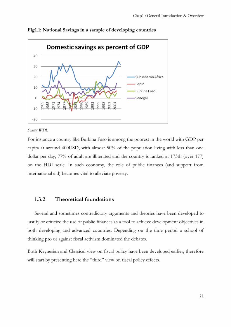
Many developing countries face the problem of a weak level of national savings. In
such situation, the scarcity of savings usually causes a drought in terms of funds necessary
to ensure investment and sustainable growth in the economy. For instance for developing
African countries (Fig1.1, except South Africa) savings (in percent of GDP) have been
progressing in a very erratic way and since 1960s remained under 20% of GDP for most
countries11. Therefore the public sector remains the main viable investor agent in such
economies.
Additional to that structural fact that remained all along the past decades, there was a
theoretical argument defending the idea that fiscal policy has to be the most important
engine for private saving. Considering that economic growth is the direct result of capital
accumulation, some analysts (influenced by growth models of Harrod & Domar types)
argued that the main role for fiscal policy was to encourage private savings and
“mobilize” and add to these savings its own “mobilization” (Tanzi, 1976). To achieve
such objective in line with these theories, the unique tool available to developing
countries‟ governments was their budget and tax policies.
Another structural aspect of developing countries‟ economies challenging their public
finances is the poverty and the private sector weakness.
11 These figures are to compare with the 37% saving rates in China, 37%, Singapore, and 34% for other
non OECD high income countries.
Chap1 : General Introduction & Overview
21
Fig1.1: National Savings in a sample of developing countries
Source: WDI.
For instance a country like Burkina Faso is among the poorest in the world with GDP per
capita at around 400USD, with almost 50% of the population living with less than one
dollar per day, 77% of adult are illiterated and the country is ranked at 173th (over 177)
on the HDI scale. In such economy, the role of public finances (and support from
international aid) becomes vital to alleviate poverty.
1.3.2 Theoretical foundations
Several and sometimes contradictory arguments and theories have been developed to
justify or criticize the use of public finances as a tool to achieve development objectives in
both developing and advanced countries. Depending on the time period a school of
thinking pro or against fiscal activism dominated the debates.
Both Keynesian and Classical view on fiscal policy have been developed earlier, therefore
will start by presenting here the “third” view on fiscal policy effects.

Chap1 : General Introduction & Overview
22
The “third” theory, the Ricardian equivalence (Barro 1974)12 states that fiscal policy has
no influence on the real economy. Basically in a “Ricardian world” any reduction of
current taxes immediately induces a (exactly) same size increase of private saving.
Therefore private consumption remains unchanged and the fiscal stimulation remaining
without any significant positive result. However this theory relies on a certain number of
assumptions that are not always true. The main assumptions are presented and discussed
below:
infinite horizon: individuals anticipating future tax increase and adjusting their
savings straightaway, following a lowering of current taxes, supposes that these
individuals have an infinite horizon. As Diamond (1965) underlines it, individuals
usually live only two periods and their utility depends only on their consumption.
In such situation reducing taxes through debt will solely profit to current active
generations since the burden of the debt will be supported by future generation.
To that criticism, Robert Barro responded arguing that the motive for current
generation increase their savings after a tax cut is rather for altruism: parents taking
advantage from the tax cut to leave more heritage to their offspring (toward future
generations). Even that response does not alleviate the criticism since heritage can
have many other motives than altruism. Among the motives for heritage on can
cite two: insurance for current generation (insurance for parents to oblige their
children to be more attentive toward them), avoid a loss of consumption due to
potential longer life length.
lump sum taxation: this assumption does not seem to hold since there might exist
a gap between tax rates with distortive effects. If that today‟s tax cut is financed by
issuance of debt, then on can considers that at maturity public authorities will need
to increase the tax rate to face their obligations. This rearrangement of the timing
of marginal taxation induces intertemporal substitution effects, alters behavior, and
so seems to violate Ricardian equivalence (Seater, 1993).
12 Since the Ricardian Equivalence theory was launched, any empirical evidence has been provided. This
could be explained by the weakness of the assumptions underlying this view (Seater 1993).

Chap1 : General Introduction & Overview
23
Risk-free environment: the Ricardian equivalence considers that individuals are
insensible toward risk. But since future income is uncertain, current generations
cannot know exactly the amount of heritage they will bequeath to their children.
Therefore as soon as households are not indifferent between supplementary
income received today after a tax cut and the income they will bequeath offspring,
Ricardian equivalence does not hold anymore.
No liquidity constraints: finally if there is a gap (even minor) between the rate at
which government borrow and the one that private agents face, the Ricardian
equivalence becomes irrelevant. Indeed if the States borrow at a lower rate
(compare to household) any tax cut, financed by public debt, is perceived as a
subsidy in favor of households.
The review of the most important assumptions underlying Ricardian Equivalence
demonstrates how difficult it can be to prove its relevance for both developing and
advanced countries. Especially the risk-free environment and the perfect credit market
assumptions do not hold at all in developing countries. As said earlier credit constraint is
so important in low income countries that smoothing consumption is very difficult.
Alongside these three theories, a fourth one has arisen: the so called anti-Keynesian fiscal
effects. Giavazzi & al. (1996) first underline the existence of anti-Keynesian and non-
linear effects of fiscal policy on private agents‟ behavior. In other words fiscal policy
could induce anti-Keynesian effects. For instance a fiscal contraction (instead of inducing
economic recession as predicted by Keynesians) might positively impact real economy
through higher private consumption. On the other hand a fiscal expansion might have
recessive impact on the economy through a decline in private consumption. These effects
were first observed in some North European countries. Indeed during early 1980s,
Denmark, Sweden and Ireland were experiencing weak economic performances and
surprisingly they decided to implement fiscal adjustment in response to such situation.
The outcome was as astonishing as the measure itself since it had an expansive effect on
the economic activity. Given that this situation does not correspond to any predication of
any known theory (Keynesian, neo-classical, Ricardian etc.), therefore this lead to the
birth of a new theory arguing that there exists some non-linearities in the behavior of
Chap1 : General Introduction & Overview
24
agents depending on the situation of public finances. The channels have been identified as
justifying such “counter-intuitive” effects of restrictive fiscal policies:
Channel of supply: the composition of the fiscal adjustment influences the
formation of agents‟ expectation on the supply side. For instance a fiscal
contraction policy that consists in reducing payment arrears will be more effective
in terms of growth enhancing. Also a fiscal restrictive policy reducing social
spending will more growth enhancing than a cut in investment budget (Baldacci et
al., 2005).
Psychological threshold: the private agents‟ perception on fiscal sustainability is an
important explanation of their own behavior. Indeed whenever tax payers consider
that public debt has reached an unsustainable level, they consider that an
adjustment (with higher tax rates) is very close and will be supported by their own
generation (Sutherland, 1995).
Channel of demand: through such channel, consumers consider fiscal contraction
measures as future lower taxes. Consequently, they can reduce their savings and
increase their expenditures, these facts ending with a stimulated economic activity
(Giavazzi & Pagano, 1990).
However few studies have tested the non-linear effects of fiscal policies in developing
countries. Among these Tanimoune & al. 2008, give evidences on the existence of “non-
conventional” fiscal effects for Western African Economic and Monetary Union
(WAEMU) countries. Relying on exogenous identification method of thresholds (Hansen
1999), they found that above a ratio of debt-to-GDP above 83% public interventions
become anti-Keynesian (expansive fiscal adjustments). Their data show that the supply
channel was the main explanation for that since for such economies fiscal adjustment very
often means reduction of payment arrears. On the same vein, Patillo & al. 2002 also
confirmed such non-linear effects of external debt in developing countries. Their first
explanation is consistent with the supply channel, higher debt discouraging for investment
(see supra). The second channel argue that in developing countries when level of debt is
very high, government has less motivated to run policy reforms (trade liberalization,
Chap1 : General Introduction & Overview
25
privatizations etc.) that would enhance growth and efficiency. The reason being that
public authorities might perceive that future benefits could be accrued by foreign lenders.
Their estimations show that when debt-to-exports ratio is above 160 – 170 percent (or for
debt-to-GDP ratio this becomes 35 – 40 percent). In terms of policy implication,
reducing debt for developing countries for example in the HIPC framework could
enhance output growth by half to 1%.
1.3.3 Limits to fiscal policy efficiency: political economy of
budget deficit
Unfortunately, and very often it happens that theoretical predications to be different
from the situation in the field in developing countries. Indeed for many developing
countries fiscal budget deficits failed to enhance output growth and these deficits by the
end of 1970s ended up with severe debts problems. For instance from Fig1.2, a simple
scatter diagram, one can see that high fiscal deficit does not guarantee output growth for
many countries (Bolivia, Nicaragua, Jamaica etc.). Fig1.3 shows a clear bias in favor of
procyclical fiscal policies for a group of developing countries: higher output gap
associated with increasing deficits (especially for Nicaragua, Malawi and Egypt (among
others) where the situation is worst since relative important fiscal deficits coexist with
weak growth performance). These observations demonstrate that fiscal policy is not that
efficient in developing countries in terms of economic stimulation. Several arguments in
the literature tried to explain such low efficiency of fiscal policies in developing countries,
in what follows two ideas are presented.
Structural Economic explanations: an important part of the literature on fiscal
issues in low income countries considers the economic structure itself as the main
limit against more efficient fiscal policies. To achieve its usual duties (provide
public goods and services) and be able to have a significant influence on the
economy, public sector needs resources. Unfortunately mobilizing both internal
and external resources is a big challenge for developing countries. Among the

Chap1 : General Introduction & Overview
26
main three resources available to developing countries tax revenue is the best way
to cover public spending (Brun & al. 2006)13. However government revenues in
developing countries suffer from two limits: its instability and weakness. The
instability of fiscal resources lowers the ability of authorities to keep sustained level
of public (Chambas 2005). Additional to that, the instability of fiscal resources is a
source of risk and higher vulnerability toward internal and external shocks. Recent
studies (Combes & Saadi-Sedik 2006 and Collier & Gunning 1999) demonstrate
the detrimental effects on fiscal budget balance and long-run growth of unstable
budgetary revenues. Among the developing world and for the period 1970-2003,
fiscal revenues instability is far more important for Sub-Saharan
Fig 1.2: Budget Deficit and Output Growth in Developing Countries: 1970-
1995
ARGARGARGARGARGARGARGARGARGARGARGARGARGARGARGARGARGARGARGARGARGARGARGARGARGARGBDIBDIBDIBDIBDIBDIBDIBDIBDIBDIBDIBDIBDIBDIBDIBDIBDIBDIBDIBDIBDIBDIBDIBDIBDIBDI BFABFABFABFABFABFABFABFABFABFABFABFABFABFABFABFABFABFABFABFABFABFABFABFABFABFA
BGDBGDBGDBGDBGDBGDBGDBGDBGDBGDBGDBGDBGDBGDBGDBGDBGDBGDBGDBGDBGDBGDBGDBGDBGDBGD
BOLBOLBOLBOLBOLBOLBOLBOLBOLBOLBOLBOLBOLBOLBOLBOLBOLBOLBOLBOLBOLBOLBOLBOLBOLBOL
BRABRABRABRABRABRABRABRABRABRABRABRABRABRABRABRABRABRABRABRABRABRABRABRABRABRABRBBRBBRBBRBBRBBRBBRBBRBBRBBRBBRBBRBBRBBRBBRBBRBBRBBRBBRBBRBBRBBRBBRBBRBBRBBRB
BWABWABWABWABWABWABWABWABWABWABWABWABWABWABWABWABWABWABWABWABWABWABWABWABWABWA
CHLCHLCHLCHLCHLCHLCHLCHLCHLCHLCHLCHLCHLCHLCHLCHLCHLCHLCHLCHLCHLCHLCHLCHLCHLCHLCOLCOLCOLCOLCOLCOLCOLCOLCOLCOLCOLCOLCOLCOLCOLCOLCOLCOLCOLCOLCOLCOLCOLCOLCOLCOL
CRICRICRICRICRICRICRICRICRICRICRICRICRICRICRICRICRICRICRICRICRICRICRICRICRICRI
DOMDOMDOMDOMDOMDOMDOMDOMDOMDOMDOMDOMDOMDOMDOMDOMDOMDOMDOMDOMDOMDOMDOMDOMDOMDOMECUECUECUECUECUECUECUECUECUECUECUECUECUECUECUECUECUECUECUECUECUECUECUECUECUECU
EGYEGYEGYEGYEGYEGYEGYEGYEGYEGYEGYEGYEGYEGYEGYEGYEGYEGYEGYEGYEGYEGYEGYEGYEGYEGY
FJIFJIFJIFJIFJIFJIFJIFJIFJIFJIFJIFJIFJIFJIFJIFJIFJIFJIFJIFJIFJIFJIFJIFJIFJIFJIGHAGHAGHAGHAGHAGHAGHAGHAGHAGHAGHAGHAGHAGHAGHAGHAGHAGHAGHAGHAGHAGHAGHAGHAGHAGHAGTMGTMGTMGTMGTMGTMGTMGTMGTMGTMGTMGTMGTMGTMGTMGTMGTMGTMGTMGTMGTMGTMGTMGTMGTMGTM
GUYGUYGUYGUYGUYGUYGUYGUYGUYGUYGUYGUYGUYGUYGUYGUYGUYGUYGUYGUYGUYGUYGUYGUYGUYGUY
HNDHNDHNDHNDHNDHNDHNDHNDHNDHNDHNDHNDHNDHNDHNDHNDHNDHNDHNDHNDHNDHNDHNDHNDHNDHNDHUNHUNHUNHUNHUNHUNHUNHUNHUNHUNHUNHUNHUNHUNHUNHUNHUNHUNHUNHUNHUNHUNHUNHUNHUNHUN
IDNIDNIDNIDNIDNIDNIDNIDNIDNIDNIDNIDNIDNIDNIDNIDNIDNIDNIDNIDNIDNIDNIDNIDNIDNIDN
INDINDINDINDINDINDINDINDINDINDINDINDINDINDINDINDINDINDINDINDINDINDINDINDINDINDIRNIRNIRNIRNIRNIRNIRNIRNIRNIRNIRNIRNIRNIRNIRNIRNIRNIRNIRNIRNIRNIRNIRNIRNIRNIRN
JAMJAMJAMJAMJAMJAMJAMJAMJAMJAMJAMJAMJAMJAMJAMJAMJAMJAMJAMJAMJAMJAMJAMJAMJAMJAM
KENKENKENKENKENKENKENKENKENKENKENKENKENKENKENKENKENKENKENKENKENKENKENKENKENKEN
KORKORKORKORKORKORKORKORKORKORKORKORKORKORKORKORKORKORKORKORKORKORKORKORKORKOR
LBRLBRLBRLBRLBRLBRLBRLBRLBRLBRLBRLBRLBRLBRLBRLBRLBRLBRLBRLBRLBRLBRLBRLBRLBRLBRLKALKALKALKALKALKALKALKALKALKALKALKALKALKALKALKALKALKALKALKALKALKALKALKALKALKA
MDVMDVMDVMDVMDVMDVMDVMDVMDVMDVMDVMDVMDVMDVMDVMDVMDVMDVMDVMDVMDVMDVMDVMDVMDVMDVMEXMEXMEXMEXMEXMEXMEXMEXMEXMEXMEXMEXMEXMEXMEXMEXMEXMEXMEXMEXMEXMEXMEXMEXMEXMEXMLIMLIMLIMLIMLIMLIMLIMLIMLIMLIMLIMLIMLIMLIMLIMLIMLIMLIMLIMLIMLIMLIMLIMLIMLIMLI MUSMUSMUSMUSMUSMUSMUSMUSMUSMUSMUSMUSMUSMUSMUSMUSMUSMUSMUSMUSMUSMUSMUSMUSMUSMUS
MWIMWIMWIMWIMWIMWIMWIMWIMWIMWIMWIMWIMWIMWIMWIMWIMWIMWIMWIMWIMWIMWIMWIMWIMWIMWIMYSMYSMYSMYSMYSMYSMYSMYSMYSMYSMYSMYSMYSMYSMYSMYSMYSMYSMYSMYSMYSMYSMYSMYSMYSMYS
NGANGANGANGANGANGANGANGANGANGANGANGANGANGANGANGANGANGANGANGANGANGANGANGANGANGA
NICNICNICNICNICNICNICNICNICNICNICNICNICNICNICNICNICNICNICNICNICNICNICNICNICNIC
NPLNPLNPLNPLNPLNPLNPLNPLNPLNPLNPLNPLNPLNPLNPLNPLNPLNPLNPLNPLNPLNPLNPLNPLNPLNPLPAKPAKPAKPAKPAKPAKPAKPAKPAKPAKPAKPAKPAKPAKPAKPAKPAKPAKPAKPAKPAKPAKPAKPAKPAKPAK
PANPANPANPANPANPANPANPANPANPANPANPANPANPANPANPANPANPANPANPANPANPANPANPANPANPANPERPERPERPERPERPERPERPERPERPERPERPERPERPERPERPERPERPERPERPERPERPERPERPERPERPERPHLPHLPHLPHLPHLPHLPHLPHLPHLPHLPHLPHLPHLPHLPHLPHLPHLPHLPHLPHLPHLPHLPHLPHLPHLPHL
PNGPNGPNGPNGPNGPNGPNGPNGPNGPNGPNGPNGPNGPNGPNGPNGPNGPNGPNGPNGPNGPNGPNGPNGPNGPNG
PRYPRYPRYPRYPRYPRYPRYPRYPRYPRYPRYPRYPRYPRYPRYPRYPRYPRYPRYPRYPRYPRYPRYPRYPRYPRYROMROMROMROMROMROMROMROMROMROMROMROMROMROMROMROMROMROMROMROMROMROMROMROMROMROM
SLBSLBSLBSLBSLBSLBSLBSLBSLBSLBSLBSLBSLBSLBSLBSLBSLBSLBSLBSLBSLBSLBSLBSLBSLBSLB
SLESLESLESLESLESLESLESLESLESLESLESLESLESLESLESLESLESLESLESLESLESLESLESLESLESLE
SLVSLVSLVSLVSLVSLVSLVSLVSLVSLVSLVSLVSLVSLVSLVSLVSLVSLVSLVSLVSLVSLVSLVSLVSLVSLV
SURSURSURSURSURSURSURSURSURSURSURSURSURSURSURSURSURSURSURSURSURSURSURSURSURSUR
SYRSYRSYRSYRSYRSYRSYRSYRSYRSYRSYRSYRSYRSYRSYRSYRSYRSYRSYRSYRSYRSYRSYRSYRSYRSYRTCDTCDTCDTCDTCDTCDTCDTCDTCDTCDTCDTCDTCDTCDTCDTCDTCDTCDTCDTCDTCDTCDTCDTCDTCDTCDTGOTGOTGOTGOTGOTGOTGOTGOTGOTGOTGOTGOTGOTGOTGOTGOTGOTGOTGOTGOTGOTGOTGOTGOTGOTGO
THATHATHATHATHATHATHATHATHATHATHATHATHATHATHATHATHATHATHATHATHATHATHATHATHATHATTOTTOTTOTTOTTOTTOTTOTTOTTOTTOTTOTTOTTOTTOTTOTTOTTOTTOTTOTTOTTOTTOTTOTTOTTOTTO
TUNTUNTUNTUNTUNTUNTUNTUNTUNTUNTUNTUNTUNTUNTUNTUNTUNTUNTUNTUNTUNTUNTUNTUNTUNTUN
URYURYURYURYURYURYURYURYURYURYURYURYURYURYURYURYURYURYURYURYURYURYURYURYURYURYVENVENVENVENVENVENVENVENVENVENVENVENVENVENVENVENVENVENVENVENVENVENVENVENVENVEN
ZMBZMBZMBZMBZMBZMBZMBZMBZMBZMBZMBZMBZMBZMBZMBZMBZMBZMBZMBZMBZMBZMBZMBZMBZMBZMB
ZWEZWEZWEZWEZWEZWEZWEZWEZWEZWEZWEZWEZWEZWEZWEZWEZWEZWEZWEZWEZWEZWEZWEZWEZWEZWE
-30
-20
-10
010
Fisc
al Bu
dget
Bala
nce
-.05 0 .05 .1Output Growth
13 Brun & al. 2006 argue that given the constraints and uncertainties on seigniorage (inflation hazard) and
grants, and the necessity to have to rely on future public revenues to be able to obtain loans, tax revenues
are the most reliable resources.

Chap1 : General Introduction & Overview
27
Fig 1.3: Budget deficit and output gap in Developing countries: 1970-1995
ARGARGARGARGARGARGARGARGARGARGARGARGARGARGARGARGARGARGARGARGARGARGARGARGARGARGBDIBDIBDIBDIBDIBDIBDIBDIBDIBDIBDIBDIBDIBDIBDIBDIBDIBDIBDIBDIBDIBDIBDIBDIBDIBDIBFABFABFABFABFABFABFABFABFABFABFABFABFABFABFABFABFABFABFABFABFABFABFABFABFABFA
BGDBGDBGDBGDBGDBGDBGDBGDBGDBGDBGDBGDBGDBGDBGDBGDBGDBGDBGDBGDBGDBGDBGDBGDBGDBGD
BOLBOLBOLBOLBOLBOLBOLBOLBOLBOLBOLBOLBOLBOLBOLBOLBOLBOLBOLBOLBOLBOLBOLBOLBOLBOL
BRABRABRABRABRABRABRABRABRABRABRABRABRABRABRABRABRABRABRABRABRABRABRABRABRABRABRBBRBBRBBRBBRBBRBBRBBRBBRBBRBBRBBRBBRBBRBBRBBRBBRBBRBBRBBRBBRBBRBBRBBRBBRBBRB
BWABWABWABWABWABWABWABWABWABWABWABWABWABWABWABWABWABWABWABWABWABWABWABWABWABWA
CHLCHLCHLCHLCHLCHLCHLCHLCHLCHLCHLCHLCHLCHLCHLCHLCHLCHLCHLCHLCHLCHLCHLCHLCHLCHLCOLCOLCOLCOLCOLCOLCOLCOLCOLCOLCOLCOLCOLCOLCOLCOLCOLCOLCOLCOLCOLCOLCOLCOLCOLCOL
CRICRICRICRICRICRICRICRICRICRICRICRICRICRICRICRICRICRICRICRICRICRICRICRICRICRI
DOMDOMDOMDOMDOMDOMDOMDOMDOMDOMDOMDOMDOMDOMDOMDOMDOMDOMDOMDOMDOMDOMDOMDOMDOMDOM ECUECUECUECUECUECUECUECUECUECUECUECUECUECUECUECUECUECUECUECUECUECUECUECUECUECU
EGYEGYEGYEGYEGYEGYEGYEGYEGYEGYEGYEGYEGYEGYEGYEGYEGYEGYEGYEGYEGYEGYEGYEGYEGYEGY
FJIFJIFJIFJIFJIFJIFJIFJIFJIFJIFJIFJIFJIFJIFJIFJIFJIFJIFJIFJIFJIFJIFJIFJIFJIFJIGHAGHAGHAGHAGHAGHAGHAGHAGHAGHAGHAGHAGHAGHAGHAGHAGHAGHAGHAGHAGHAGHAGHAGHAGHAGHAGTMGTMGTMGTMGTMGTMGTMGTMGTMGTMGTMGTMGTMGTMGTMGTMGTMGTMGTMGTMGTMGTMGTMGTMGTMGTM
GUYGUYGUYGUYGUYGUYGUYGUYGUYGUYGUYGUYGUYGUYGUYGUYGUYGUYGUYGUYGUYGUYGUYGUYGUYGUY
HNDHNDHNDHNDHNDHNDHNDHNDHNDHNDHNDHNDHNDHNDHNDHNDHNDHNDHNDHNDHNDHNDHNDHNDHNDHNDHUNHUNHUNHUNHUNHUNHUNHUNHUNHUNHUNHUNHUNHUNHUNHUNHUNHUNHUNHUNHUNHUNHUNHUNHUNHUN
IDNIDNIDNIDNIDNIDNIDNIDNIDNIDNIDNIDNIDNIDNIDNIDNIDNIDNIDNIDNIDNIDNIDNIDNIDNIDN
INDINDINDINDINDINDINDINDINDINDINDINDINDINDINDINDINDINDINDINDINDINDINDINDINDINDIRNIRNIRNIRNIRNIRNIRNIRNIRNIRNIRNIRNIRNIRNIRNIRNIRNIRNIRNIRNIRNIRNIRNIRNIRNIRN
JAMJAMJAMJAMJAMJAMJAMJAMJAMJAMJAMJAMJAMJAMJAMJAMJAMJAMJAMJAMJAMJAMJAMJAMJAMJAM
KENKENKENKENKENKENKENKENKENKENKENKENKENKENKENKENKENKENKENKENKENKENKENKENKENKEN
KORKORKORKORKORKORKORKORKORKORKORKORKORKORKORKORKORKORKORKORKORKORKORKORKORKOR
LBRLBRLBRLBRLBRLBRLBRLBRLBRLBRLBRLBRLBRLBRLBRLBRLBRLBRLBRLBRLBRLBRLBRLBRLBRLBRLKALKALKALKALKALKALKALKALKALKALKALKALKALKALKALKALKALKALKALKALKALKALKALKALKALKA
MDVMDVMDVMDVMDVMDVMDVMDVMDVMDVMDVMDVMDVMDVMDVMDVMDVMDVMDVMDVMDVMDVMDVMDVMDVMDVMEXMEXMEXMEXMEXMEXMEXMEXMEXMEXMEXMEXMEXMEXMEXMEXMEXMEXMEXMEXMEXMEXMEXMEXMEXMEX MLIMLIMLIMLIMLIMLIMLIMLIMLIMLIMLIMLIMLIMLIMLIMLIMLIMLIMLIMLIMLIMLIMLIMLIMLIMLIMUSMUSMUSMUSMUSMUSMUSMUSMUSMUSMUSMUSMUSMUSMUSMUSMUSMUSMUSMUSMUSMUSMUSMUSMUSMUS
MWIMWIMWIMWIMWIMWIMWIMWIMWIMWIMWIMWIMWIMWIMWIMWIMWIMWIMWIMWIMWIMWIMWIMWIMWIMWIMYSMYSMYSMYSMYSMYSMYSMYSMYSMYSMYSMYSMYSMYSMYSMYSMYSMYSMYSMYSMYSMYSMYSMYSMYSMYS
NGANGANGANGANGANGANGANGANGANGANGANGANGANGANGANGANGANGANGANGANGANGANGANGANGANGA
NICNICNICNICNICNICNICNICNICNICNICNICNICNICNICNICNICNICNICNICNICNICNICNICNICNIC
NPLNPLNPLNPLNPLNPLNPLNPLNPLNPLNPLNPLNPLNPLNPLNPLNPLNPLNPLNPLNPLNPLNPLNPLNPLNPLPAKPAKPAKPAKPAKPAKPAKPAKPAKPAKPAKPAKPAKPAKPAKPAKPAKPAKPAKPAKPAKPAKPAKPAKPAKPAK
PANPANPANPANPANPANPANPANPANPANPANPANPANPANPANPANPANPANPANPANPANPANPANPANPANPAN PERPERPERPERPERPERPERPERPERPERPERPERPERPERPERPERPERPERPERPERPERPERPERPERPERPERPHLPHLPHLPHLPHLPHLPHLPHLPHLPHLPHLPHLPHLPHLPHLPHLPHLPHLPHLPHLPHLPHLPHLPHLPHLPHLPNGPNGPNGPNGPNGPNGPNGPNGPNGPNGPNGPNGPNGPNGPNGPNGPNGPNGPNGPNGPNGPNGPNGPNGPNGPNG
PRYPRYPRYPRYPRYPRYPRYPRYPRYPRYPRYPRYPRYPRYPRYPRYPRYPRYPRYPRYPRYPRYPRYPRYPRYPRYROMROMROMROMROMROMROMROMROMROMROMROMROMROMROMROMROMROMROMROMROMROMROMROMROMROM
SLBSLBSLBSLBSLBSLBSLBSLBSLBSLBSLBSLBSLBSLBSLBSLBSLBSLBSLBSLBSLBSLBSLBSLBSLBSLB
SLESLESLESLESLESLESLESLESLESLESLESLESLESLESLESLESLESLESLESLESLESLESLESLESLESLE
SLVSLVSLVSLVSLVSLVSLVSLVSLVSLVSLVSLVSLVSLVSLVSLVSLVSLVSLVSLVSLVSLVSLVSLVSLVSLV
SURSURSURSURSURSURSURSURSURSURSURSURSURSURSURSURSURSURSURSURSURSURSURSURSURSUR
SYRSYRSYRSYRSYRSYRSYRSYRSYRSYRSYRSYRSYRSYRSYRSYRSYRSYRSYRSYRSYRSYRSYRSYRSYRSYRTCDTCDTCDTCDTCDTCDTCDTCDTCDTCDTCDTCDTCDTCDTCDTCDTCDTCDTCDTCDTCDTCDTCDTCDTCDTCD TGOTGOTGOTGOTGOTGOTGOTGOTGOTGOTGOTGOTGOTGOTGOTGOTGOTGOTGOTGOTGOTGOTGOTGOTGOTGO
THATHATHATHATHATHATHATHATHATHATHATHATHATHATHATHATHATHATHATHATHATHATHATHATHATHA TTOTTOTTOTTOTTOTTOTTOTTOTTOTTOTTOTTOTTOTTOTTOTTOTTOTTOTTOTTOTTOTTOTTOTTOTTOTTO
TUNTUNTUNTUNTUNTUNTUNTUNTUNTUNTUNTUNTUNTUNTUNTUNTUNTUNTUNTUNTUNTUNTUNTUNTUNTUN
URYURYURYURYURYURYURYURYURYURYURYURYURYURYURYURYURYURYURYURYURYURYURYURYURYURY VENVENVENVENVENVENVENVENVENVENVENVENVENVENVENVENVENVENVENVENVENVENVENVENVENVEN
ZMBZMBZMBZMBZMBZMBZMBZMBZMBZMBZMBZMBZMBZMBZMBZMBZMBZMBZMBZMBZMBZMBZMBZMBZMBZMB
ZWEZWEZWEZWEZWEZWEZWEZWEZWEZWEZWEZWEZWEZWEZWEZWEZWEZWEZWEZWEZWEZWEZWEZWEZWEZWE
-30-20
-10
010
Fisca
l Bud
get B
alanc
e
-5.00e-10 0 5.00e-10 1.00e-09 1.50e-09Output Gap
African countries especially for the Least Developed Countries group (Brun & al.
2006). Now regarding the second characteristic of public revenues in the
developing world, Brun & al. 2006 developed a new framework to assess its
weakness. They define the fiscal effort as the difference between resources actually
mobilized and the potential fiscal revenues. The potential fiscal revenue is an indicator
representing public resources that depend on structural characteristic of the
economy. The fiscal effort captures the extent to which the public sector feats its
potential revenues (positive values of fiscal effort show up the fact that potential
resources are fully used). Their results (Brun & al. 2006) shows that for developing
countries, except for North-African and Middle East countries, fiscal effort is very
low especially for Least Developed countries where it is negative. The dependence
toward trade on primary commodities and international development aid are
among the main causes of government revenues instability (Brun & al. 1999). The
important share of the unregistered sector in developing countries (despite its
important economic role: for instance in a county like Niger up to 50% of jobs
created are in the unregistered sector, Chambas 2010) also contribute to weaken
the revenues the public sector can raise. Therefore is becomes easily
understandable why fiscal policy cannot play its role (of providing with public
goods, stabilize macroeconomic fluctuations and alleviate poverty) in low income

Chap1 : General Introduction & Overview
28
countries. Fiscal decentralization, an area in public economics still growing up, has
been considered as a credible answer to the limits that prevent fiscal policy from
being more efficient. A closer fiscal management could help to raise more tax
revenues and also encourage the delivery of timely and better public goods that
population need.
Political Economy of fiscal budget balance: inefficiencies of fiscal policies have
been assigned to institutional weaknesses. Indeed due to agency problems, public
authorities might try to influence citizens‟ perception and let them believe that the
current government is highly competent. Pioneered by Nordhaus (1975), the
political business cycle theory states that the renewal of public authorities might
have an impact on the real economy. Indeed in countries where elections take
place the incumbent in order to remain in power might increase its delivery of
public goods. For developing countries it has been proved that political budget
cycles do exist since during elections budget deficit worsens (Brender & Drazen
2005, Schuknecht 1996). Shi & Svensson (2006) found that on average budget
deficit increase by 1% of GDP in election periods. Despite this evidence of
political budget cycles presence in developing countries, some criticisms have
raised two limits against that theory. The first one underlines the fact that these
budget cycle models are not suitable to all developing countries and the situation is
completely different according to the “deepness of the democracy”. In countries
where democracy is well established fiscal manipulations are punished by voters; in
such countries citizens have a better sight on political economy instruments
(Brender & Drazen, 2005 found a clear difference in the magnitude of political
budget cycles between countries when one separates new democracies and
established ones). The second limit is in straight line with our main concern: do
political budget cycles undermine the efficiency of fiscal policy? One could
reasonably imagine that, even if deficits increase sharply during a given period of
time (this is referred here as elections), fiscal authorities might use these extra-
spending for efficient and productive investments that would enhance future
growth. Therefore one needs to go even further in the analysis to see the
composition of public spending in election‟s period. Theoretically, Rogoff (1990)

Chap1 : General Introduction & Overview
29
developed a signaling model where political budget cycles are caused by
information asymmetries. Since spending on public goods is a signal of the
incumbent‟s competence (just before elections), the government will prefer to run
current spending that are quickly visible to voters (usually for capital spending one
gets the returns during the next period). These current spending mainly covers
salaries, subsidies on final consumption goods etc. Block (2002) will confirm these
theoretical predications from a panel of 69 developing countries that during
election periods (a year before the race), incumbents increase current expenditures
and usually capital ones are neglected or lowered. Finally it comes out that
politico-economic cycle is another important limitation to fiscal policy efficiency in
developing countries.
The upper analyses shed light on the causes (at least some of them) that explain the
reason why fiscal policy in developing countries could not achieve its goals (see supra), or
even be a counter-productive political economy tool.
This dissertation aims at contributing to the literature of fiscal policies in developing
countries though focusing mainly on its effects and from there to be able to deliver policy
recommendations in order to improve the matter. Before coming into details to the
content of this dissertation, some other key uses and features of fiscal policy will be
reminded.
1.4 Overview on the Rationale of the importance of Fiscal Policies in developing countries.
The previous sections help to understand some of the main characteristics and
limitations of fiscal efficiency in developing economies. Even if it comes out from upper
analysis that there exist several economic to political factors that refrain budget policies to
reach their objective, one still need to further shed light on which specific areas fiscal
policy might be helpful in the economic development process. To do so, a short review
on theories on the linkages between public budget and specific economic aggregate will

Chap1 : General Introduction & Overview
30
be developed. Additional to that, it would be interesting for our purposes to investigate
new policies being implemented in many low income countries and (both national and
those accompanied by international development partners) aimed at improving public
finances‟ efficiency.
1.4.1 Fiscal theory for price level
The fiscal theory of price level (FTPL) initiated by Leeper (1991) Sims (1994) and
Woodford (1994), states that the quantity theory of money (QTM) is not enough to
explain the dynamics of price level in a country. The main contribution for this theory is
to argue that price level is determined by the level of public debt. For instance Turkey had
experienced severe episodes of hyperinflation during early 1980s and late 1990 despite a
relative monetary policy discipline (the seigniorage to GDP ratio have remained very low
and were even declining)14. In countries were fiscal policy is non-Ricardian (namely public
debt is not neutral) and if fiscal policy is dominant15 then anti-inflationary monetary
policies will be inefficient or worse they can be inflationary (Benhabib & al. 2001). Fiscal
policy impacts on price level mainly through the wealth effects related to the issuance of
domestic debt. As Woodford (2001) underlines it, in economies where fiscal policy is
dominant primary deficit directly causes the level of public debt and the borrowing
requirement to increase. If government mainly recourses to domestic borrowing it is most
than likely cost of borrowings will go up (interest rates and risk premiums). Therefore a
strong wealth effect can lead to inflation since domestic creditors feels wealthier. For the
Turkish case additional to these channels detailed, the maturity rate on domestic debt
keeps getting shorter and shorter during the mid-1980 and late 1990s, worsening the
inflation pressure. Hence monetary policies especially inflation targeting to be effective
absolutely needs to be accompanied by accommodating fiscal behavior (Favero &
14 In 1984 and 1996 the inflation rate in Turkey was 140% and 130%.
15 Fiscal policy is dominant when monetary policy accommodates fiscal decisions. In such situation
monetary policy will consider fiscal policy as a constraint in the political decision process (Woodford
1994).

Chap1 : General Introduction & Overview
31
Giavazzi 2002). For developing countries this theory is an important matter directly
related to their macroeconomic stability. Indeed governments as well as international
development partners and academics are advocating for a deeper development of the
financial sector for developing economies. The argument underlying such views is that
external financing possibilities are getting scarcer for low (and middle) income countries
therefore it becomes essential to be able to raise domestic finds. Any policy in favor of
financial sector development should consider first the necessity for fiscal authorities to
run prudential policies. In other words any pro-financial sector development policy might
be destabilizing for poor countries if it ends up with government borrowing domestically
at unreasonable level leading to higher level of inflation (that is harmful especially to the
poorest agents).
1.4.2 Current account targeting
This theory is an extension of the twin deficit debate. A large section of academic
studies have been interested in the relationship between external and budget deficits.
Most empirical studies state the positive correlation and the comovement between
external and budget deficits for developing countries (Chinn & Prasad 2003, Calderon &
al. 2002). This positive comovement has been firstly explained by the relation between
current account, private saving and budget balance16. Beyond this arithmetic relationship
between external (current account) deficit and budget imbalance, shock associated with
internal conditions (especially domestic resources net of public absorption) are the most
important factor that explain the comovement between the two deficits (Chichi &
Normandin 2008). Therefore if this relation becomes well established fiscal policy can be
used by developing countries to sort out part of their economies‟ intertemporal budget
constraint. In other words as developing countries mainly rely on external debt; they
cannot afford to run indefinitely current account deficit since this debt needs to be repaid
16 G p pCA S I CA S S I CA T G S I , with CA the current
account balance, pS private saving, GS public saving, I investment, T government revenues, G public
spending.

Chap1 : General Introduction & Overview
32
one day or another. Therefore in case current account threatens intertemporal solvency
condition, the government is likely to use its budget (by increasing public savings) to
adjust the external balance. Hence international debt relief initiatives and also
concessionary should bear in mind that helping countries to overcome their balance of
payments turmoil should not encourage fiscal authorities to run loose policies. Removing
such constraint (external imbalance) for developing economies‟ government, should not
encourage moral hazard behavior that could end up with (once again) inefficient fiscal
policies. The only bottom line is that this issue has not been widely covered in the
empirical literature, further investigations might allow seeing whether (some) developing
countries really use budget variables to target current account balance. In order to capture
the potential current account targeting and avoid bias in our estimations, the external
sector (current account balance) will be considered in our empirical strategies all along
this dissertation.
Recent international initiatives initiated by Bretton-Woods institutions have been focusing
on ways and means to implement deep reforms in the budget area in low income
countries.
1.4.3 The Medium Term Expenditure Framework: a new tool for better budget practices
Developing countries especially low incomes ones suffers from inefficient use of
budgetary items. In the context where international development aid and proceeds from
potential exportations are scarce and volatile, to achieve economic development and
alleviate poverty public revenues and expenditures have to be efficient. In this context,
several developing countries in partnership with multilateral development agencies (World
Bank, IMF and, joined later by bilateral partners) have launched reforms on the public
finance management (PFM). The PFM is a wide initiative (launched by World Bank)
aimed at improving institutional arrangement and management practices that would create
an environment favorable to better resource allocation, resource use and disciplined
financial management. The departure point of this initiative has been the argument that

Chap1 : General Introduction & Overview
33
poor institutional arrangements are the main cause of undisciplined fiscal policy with
adverse consequence on most vulnerable in the economy. Additional to that, recent
analysis directly links ineffective budgeting systems and inappropriate, unsustainable
policy choices and sector allocations on one hand and links also poor budgeting systems
and weak policy implementation and inadequate service delivery (Le-Houerou & Taliercio
2002). In the PFM framework to be successful public finances reforms require to build up
bridges between three levels of budgetary outcomes aggregate fiscal discipline, allocation
of resources in accordance with strategic priorities and finally efficient and effective use of
resources in the implementation of strategic priorities (World Bank 2002). Once the
overall outcomes expected from these reforms, public expenditure reviews (PER) in
developing countries ended up suggesting the adoption of medium-term expenditure
frameworks (MTEF). The MTEF consists of a top-down resource envelope, a bottom-up
estimation of the current and medium-term costs of existing policy and, ultimately, the
matching of these costs with available resources in the context of the annual budget
process (World Bank 1998). In other words under MTEF expenditures are solely driven
by policy priorities. In the context of developing countries one first develops a
macroeconomic and fiscal model that will provide with forecast of revenues and
expenditures. Then development strategies and expenditure needs are identified for each
(important) sector. This later document will be adopted by authorities as the final MTEF
(Table1.1). Since early 1990s, MTEF has been rapidly adopted across the developing
world (just between 1997 and 2001 more than 25 countries adopted the MTEF reform).
Even if these figures might be interpreted as a success for PEM initiative, there has not
been done yet an empirical assessment of the MTEF policies. Future studies could run
macro-impact analysis and see whether these amendments have been successful in helping
budgetary policies to targeting social and pro-poor expenditures.
The next section will present the rationale of this dissertation

Chap1 : General Introduction & Overview
34
Table 1.1 The Different Stages of a MTEF
STAGE CHARACTERISTICS
I. Development of Macroeconomic/Fiscal Framework
Macroeconomic model that projects revenues and expenditure in the medium term (multi-year)
II. Development of Sectoral Programs
Agreement on sector objectives, outputs, and activities
Review and development of programs and sub-programs
Program cost estimation
III. Development of Sectoral Expenditure Frameworks
Analysis of inter- and intra-sectoral trade-offs
Consensus-building on strategic resource allocation
IV. Definition of Sector Resource Allocations
Setting medium term sector budget ceilings (cabinet approval)
V. Preparation of Sectoral Budgets Medium term sectoral programs based on budget ceilings
VI. Final Political Approval Presentation of budget estimates to cabinet and parliament for approval
Source: PEM Handbook (World Bank, 1998, pp. 47-51).
1.4.4 Contribution of this PhD dissertation and details
on the content
The first chapter has been dedicated to first present key and commonly used fiscal
concepts. These aggregates and concepts will be used all along the three remaining
chapter to explain the phenomenon will be focusing on.
In a first stance this review indicated that developing countries especially low income ones
have been running unsustainable fiscal policies. Debt levels had reached certain threshold
that made compulsory adjustment and debt relief programs. Despite such indebtedness
the success of fiscal policy in terms of poverty alleviation, output growth, employment
and poverty reduction has been extremely modest. Given that traditional theories on
fiscal policy failed to explain such situations, we have investigated the other arguments.
“Structural Economic explanation” has argued that fiscal policy is neutral toward its
objective due to the economic structures (large unregistered sector, weak tax revenues,
scarcity of external resources etc.). On the other hand political economy theories argue
that the strength of fiscal institutions and all political institutions in general has been the
main cause of such underperformances of fiscal policies.

Chap1 : General Introduction & Overview
35
The common point between these different observations is that fiscal policy in
developing countries is an essential component in the development process and ignoring
or imposing unreasonable fiscal discipline could threatens its main objectives. The second
and very obvious observance is that public finances are not “healthy” in these economies.
However studies focusing on the empirical analysis of fiscal effects in developing
countries have remained scarce. First of all studying fiscal policy effect for developing
countries requires the use of relevant statistical tools and assumption since these
economies are quite different from what can be seen in their developed counterparts. The
literature survey has shown that several recesses up to now have not been investigated.
This dissertation overarching aim will be, through three fields of analysis, provide a better
understanding of fiscal policies effects in developing and show how the situation has
changed over years.
Chapter 2: Fiscal Policy Shocks in Developing Countries: A panel SVAR approach
The literature on fiscal policies effects has mainly covered three aspects. The first aspect
(see supra) focused on the taxation system and the inefficiencies related to tax revenues
collection. Secondly institutional aspects characterizing budget policies, especially political
budget cycle theories have been developed and empirically tested. Finally the third group
of research wonders what would be the effects if developing countries decide to use fiscal
policy in order to influence the real economy. The responses to such question have been
inspirited by “traditional” theories (Keynesians, neo-classicals) and recent analysis has
proven non-linear relationship between fiscal variables and agents‟ responses to fiscal
stimulus (see supra). However it can reasonable happen that a (developing countries‟)
government tries to run surprise policies in order to avoid adverse agents‟ anticipations
and adaptation. Only limited empirical studies are related to this issue of the impact of
non-anticipated fiscal measures. In additional, only little attention has been dedicated to
developing economies (compare to OECD countries especially the US economy on
which several articles focused on). Schclarek 2010 on a panel of 21 developing countries
showed that spending shocks have Keynesian effect while tax shocks also have Keynesian
impact on private consumption. Nevertheless these results raise important questions

Chap1 : General Introduction & Overview
36
regarding both the identification method and the underlying assumptions. The two steps
estimation strategy, using IV-GMM (Generalized Method of Moments) does not
guarantee the clear identification of exogenous and unanticipated changes in taxes and
government spending. Also the definition of public revenues restricted to the (poor) tax
revenues neglect essential aspect of budget characteristics in developing countries. The
aim of this chapter will be, using original identification method, to answer whether
government can reasonably recourse to “surprise policies” as an efficient tool to positively
influence the real economy (and avoid adverse anticipations from private agents)?
Chapter3: Impact of Large Fiscal Imbalance in Advanced Countries on
Developing Countries
For developing economies it has been largely demonstrated in several articles that they are
closely related to business cycles in advanced economies. The change in exchange rate,
output growth, interest rates in western countries and their influence on the global
economy are the commonly effects studied. The consequences of developed countries‟
fiscal policies on their developing counterparts have received less attention. On the other
hand since early 1990s, after the debt crisis, fast growing “new economies” start receiving
important and capital flows. The several crises that emerging economies experienced
during the last decade of the twentieth century demonstrated how these emerging markets
were dependent toward external financing. During 2008 the new financial crisis whose
origins lie in industrial countries affected the world economy. Among the solutions
advocated by international organizations (IMF, G20, World Bank), there was the use of
fiscal stimulus I order to mitigate the systemic risk related to the “too big to fail”17. Hence
leading world economies (USA, European Union countries) engaged in important public
spending in order to keep macroeconomic stability. The third chapter investigates
whether it is reasonable to worry about a potential “world crowding out effect”.
17 In a famous article in the Financial Times Oct.2009 (“How the Fed Can Avoid the Next Bubble”)
Nouriel Roubini states that the stimulus packages might induce moral hazard and encourage risky
strategies by large firms (e.g. General motors, Northern Rock) that believe that they are Too Big to Fail.
Simply because the systemic risk that the collapse of such firms might cause is too important.

Chap1 : General Introduction & Overview
37
Advanced countries engaged into important public spending and increase their debt levels
in the same vein might compete with developing economies in terms of access to capital
flows. Another possible fact could be that emerging economies are entering into a new
paradigm where they are getting disconnected from business cycles in the rich world.
Chapter 4: Fiscal Policy for Stabilization in Developing Countries
Despite the well known limitations of fiscal policies in developing countries does still
public authorities tries to use it in order to stabilize macroeconomic fluctuations? Or
rather governments simply run procyclical policies as the majority of empirical analyses
argue. Indeed for these analysts, developing countries‟ fiscal authorities usually increase
their delivery of public goods (and lower taxation) in good times and run the inverse
policy in bad economic periods. This ends up worsening the severity of economic
downturns. Some authors (e.g. Carmignani 2010) fiscal policy in developing countries has
remained invariably procyclical since 1960s. Especially Carmignani 2010 who studied this
on a panel of 37 African countries found that since 1960 all these governments keep
running strong procyclical policies and a fortiori they did not learn from past situations and
crises. However the recent IMF‟s Regional Economic Outlook report in April 2010
(dedicated to Sub-Saharan African economies) calls into question these results. It has
been found during the 2010 global economic crisis that low income countries had
adopted counter-cyclical fiscal policies. Therefore a doubt arises on the validity of
Carmignani 2010 (and those sharing the same thought) findings. The last chapter
overarching aim is to show, on a yearly basis, how fiscal policies have been used in
developing economies (both Africans and Latin-Americans). Our analysis will also
address the question that is usually neglected: are procyclical fiscal policies as bad as we
might think?

Chap2: Fiscal Policy Shocks in Developing Countries: a Panel SVAR Approach
38
Chap2: Fiscal Policy Shocks in Developing Countries: a Panel SVAR Approach
39
Chapter 2: Fiscal Policy
Shocks in Developing
Countries: A Panel Structural
VAR Approach
Chap2: Fiscal Policy Shocks in Developing Countries: a Panel SVAR Approach
40
2.1 Introduction
The effects of fiscal policy is one of the most important and controversial issues in
macroeconomics. Furthermore it would be interesting to study the outcome of a sudden
and unexpected change in the fiscal policy for both developing and advanced economies.
This chapter investigates the effects of government revenue and spending shocks on
private consumption, output, external sector competitiveness and on trade balance. To
study such effects one can use the narrative approach or the Vector Autoregressive
method (VAR).
In the narrative approach, the studies on fiscal policy effects pose the hypothesis that a
decision relating to public finance taken during period t-1 is not made public until period
t. But this hypothesis is not strong enough since it is rare for a decision of this type to be
taken without any debate taking place either through the parliament or through the media.
Therefore economic agents anticipate the decision from the government and adapt their
behaviour. So the anticipation and adaptation from economic agents introduce a bias in
the identification of the effects of the fiscal change. According to Poterba (1988) (other
authors such as Leeper (1989) present a similar argumentation) if the effectiveness of a
policy is low, there is no way of verifying whether this is partially due to anticipation by
economic agents. But another theory led by Blanchard & Perotti (2002) demonstrates that
this judgment is not immutable and that by using VAR estimation it is possible to identify
exogenous (thus, unanticipated) impacts on budgetary policy.
Sims (1980) first formulated the basis for the VAR modelling. The modelling came from
the critiques against the theoretical restriction imposed on structural econometrics
(especially multi-equations modelling). These critiques concern the simultaneous
equations bias that resulted from the correlation of error terms with some explanatory
variables and the causality problem between variables. Indeed the endo versus exogenous
division of variables could lead to a bias as some variables could have reciprocal effects
(Charemza & Deadman 1992). VAR modelling considers first that there is no endo-
exogenous division of variables and second, the random errors are assumed to be

Chap2: Fiscal Policy Shocks in Developing Countries: a Panel SVAR Approach
41
contemporaneously correlated but not autocorrelated. Since this system can be estimated
consistently by ordinary least squares, VARs can be used for forecasting and analyzing
causal relationship between variables. In order to make causal inference, some changes
must be introduced in the VARs and this is called Structural Vector Autoregressions
(SVARs). The main difference between SVARs and VARs is that the structural modelling
requires very specific assumptions of what is exogenous or not (Stock & Watson 2007).
And by putting some restrictions in the SVAR one can identify the impact of
unanticipated fiscal or monetary policies. However VARs have received some strident
criticisms for its atheoretical approach, due to the unrestricted nature of the lag structure
that could be synonymous with unstructured18 (Greene, 2008). The answer given by VAR
users is that people should consider VAR models as reduced forms of a dynamic
structural model (Diebold, 1998). Hence, in order to interpret VAR outcomes, one will
need first to shed light on the theory underlying the model. This modelling method is
usually used for monetary policy forecasting. But, according to Blanchard & Perotti
(2002), the SVAR approach seems to be more suitable in fiscal policy analysis to the
extent that there exist some genuine exogenous fiscal shocks (not due to output
stabilization) and, decision and implementation lags in fiscal policy imply that there is little
discretionary response (within a quarter) to unexpected movements in activity. It was in
this context that some researchers began studying the impulse response to fiscal policy,
but this was done mostly for industrialized countries.
The objective of this chapter is twofold. First, it fills this gap for developing countries by
studying the outcome on economic activity from sudden change in the budget stance. In
addition, developing countries are highly vulnerable and subject to several external and
internal shocks. Furthermore public finances are one of the main channels through which
these shocks impact on the real economy. Indeed, due to some fiscal weaknesses (this
issue is covered in the first and fourth chapter) very often in low and middle income
countries both public expenditures and revenues exacerbate cyclical downturns. The
second objective is to investigate, in comparison to previous studies, whether developing
countries follow the same behaviour in terms of fiscal shocks as their developed
18 This would mean that there is no theoretical background under the choice of lags.

Chap2: Fiscal Policy Shocks in Developing Countries: a Panel SVAR Approach
42
counterparts. We expect from the empirical results to answer the question whether
developing countries can reverse the negative effects of shocks on the real economy.
I use SVAR with a panel of developing countries and the results show that a government
spending shock has a positive effect on output, government revenue and private
consumption. The impulse response of the external sector appears not to be statistically
significant. Explanations of these results will be given taking into account the
characteristics of developing countries.
This study is organized around five sections. The following section covers the related
literature. Section three details the model specification while the fourth section presents
the data and the forecasting results. The fifth section provides some discussion on the
results. The last part concludes.
2.2 Fiscal policy effects in the literature
Literature on fiscal policy is divided in two areas. The first deals with fiscal policy
effects without mention of the “unanticipated” aspects. The second set of studies deal
with the latter, with recourse to different methods. This section will therefore initially
cover the narrative approach of fiscal events before presenting studies and methods
aimed at solving the identification problem.
2.2.1 Narrative approach
In their study, Ramey & Matthew (1998) first define the date at which agents learn
about the upcoming increase in government expenditures. They identify three dates
(1950: Q3; 1965: Q1 and 1980: Q1) associated to some important military spending19 (and
some authors add 2001:Q4 to the list of dates on which news about expansionary defence
19 These dates correspond respectively to the Korean War, the Vietnam War and the Carter-Reagan
defence program.

Chap2: Fiscal Policy Shocks in Developing Countries: a Panel SVAR Approach
43
spending arrived after the September 11th attacks). They find that government spending
starts rising only two or three quarters after the dates identified above (Burnside & al.,
2004 reach the same conclusion) and the maximum value is reached after 6 quarters
(Ramey & Matthew 1998). So, one cannot directly compare the SVAR method and the
narrative approach as the latter only identifies anticipated changes in fiscal policy while
SVAR shows government spending innovations that are orthogonal to past information.
Using a simple model, which takes into account both unanticipated and anticipated
innovation in government purchases, confirms the above results. The explanation given is
that when agents learn about the increase in government spending in period zero, this
creates a negative wealth effect (a decrease in private consumption). Firms will hence
increase their prices to cover the “loss” in demand and obtain more profit. But in period
two, when the measure is effective, firms on the domestic market expect higher demand
and low markups. It is therefore optimal for them to disinvest in domestic market share
whereas it is optimal for firms on the foreign market to invest on this market as markups
are expected to increase in the future. In their paper, Ravn & al. (2007) reconcile the two
methodologies and show that the only difference in the results between the SVAR
method and the narrative approach is due to the behaviour of agents depending on when
they know about the change in fiscal policy.
However studies on fiscal policy effects using SVAR (or even simple VAR) on panel data
are quite rare certainly owing to the challenge associated with the identification strategy.
Despite that, after presenting some analyses using time series data in the next sub-section
the following one will review other studies on fiscal policy effects using panel data.
2.2.2 Literature on fiscal policy shocks
Blanchard & Perotti (2002) using a four-variable SVAR model on US quarterly
data of government spending, taxes, output and its components find that positive
government spending shocks have positive effects on output. The effects are completely
different after a government revenue shock, as output and public spending decrease. A
structural decomposition is implemented in order to identify unanticipated shocks. The

Chap2: Fiscal Policy Shocks in Developing Countries: a Panel SVAR Approach
44
method of identification used relies on theory and institutional information. So, for
instance, Blanchard & Perotti (2002) postulate that government spending responds with
at least a one-quarter lag to structural innovations other than innovations to government
spending itself. In other words, within a quarter only government spending can influence
itself. After defining the reduced-form residuals as a linear combination of the structural
innovations, they estimate all coefficients of those equations. For the remaining
coefficients they could not estimate (the structural innovations), they therefore imposed
some restrictions. The main limit of their study is that they do not give any explanation or
channel of transmission to explain the impulse responses of American economy to a fiscal
shock. Even if some other studies are applied to the USA, the comparison with Blanchard
& Perotti (2002) will be confined to the “statistical” outcomes and to the identification
method used. The other studies presented below try to offer a wider analysis framework.
2.2.2.1 Use of panel data
Ravn & al., (2007) use a panel SVAR of five variables for four advanced
economies. Using the Blanchard & Perotti (2002) identification strategy, they find for four
industrialized countries (United States, United Kingdom, Canada and Austria) that
unanticipated government spending shocks lead to an increase in output and private
consumption and a deterioration in the trade balance. Perotti (2004; 2007) finds the same
results. Ravn & al., (2007) go a little bit deeper in comparison to some other studies
(except Monacelli & Perotti, 2006) in the sense that they look at the effects of the increase
in government purchases on the competitiveness of the country compared to its trade
partners. The results show that a positive shock in government spending causes a quite
persistent depreciation of the real exchange rate implying that the domestic prices become
cheaper than the foreign prices. This could be a little bit astonishing, but the authors
develop a model based on “deep habit” mechanism to give a theoretical explanation of
their findings. Under deep habits, after a positive shock of government expenditures, the
resulting increase in aggregate demand gives an incentive to firms to reduce their markups
(as they can sell more and get more revenue). Then the domestic prices become inferior

Chap2: Fiscal Policy Shocks in Developing Countries: a Panel SVAR Approach
45
in relation to foreign prices and the real exchange rate declines. As a consequence of the
increase in labour demand the real wage rises. And here, one can deduct that there will be
an equilibrium increase in private consumption as the substitution effect and the wealth
effect will compensate. After an empirical test, the deep habit model confirms all the
predictions and hence is a good theoretical framework of what is observed in developed
countries when government spending increases. Therefore a key issue will be to see
whether these deep habit model predictions are relevant for developing countries. Ravn &
al., (2007) also reconcile the two ways of measuring the effects of fiscal policy, the SVAR
approach and the narrative method pioneered by Ramey & Matthew (1998). The
difference in results between the two methods solely depends on whether the change is
anticipated or not. Studies relying on the SVAR method (most of them use the Blanchard
& Perotti 2002 identification strategy) basically consider that the change in government
expenditure is unanticipated whereas the narrative approach only considers anticipated
changes, hence one should not expect the same result from the two analyses. The main
finding from the narrative approach is that a government positive spending shock fails to
cause an increase in private consumption.
2.2.2.2 Back to fiscal policy shocks
Mountford & Uhlig (2005) study the fiscal policy shocks on US quarterly data from
1955 to 2000. They use a different identification method from what is available in the
literature on fiscal policy shocks. First they define fiscal policy shock as the linear
combination of two basic shocks, the government revenue shock and the government
spending shock20. Their identification methodology mainly tries to distinguish the genuine
fiscal policy shocks from movement in fiscal variable in response to business cycles or
monetary policy shocks by only using macroeconomic quarterly data (no assumptions on
coefficient and on series). The first problem they address is the effects of the plausible lag
20 Government spending shock is defined as a shock where government spending rises for a defined
period following which a distinction between anticipated and unanticipated fiscal policy measures can be
made.

Chap2: Fiscal Policy Shocks in Developing Countries: a Panel SVAR Approach
46
between the announcement and the implementation of the policy (this can bias the result
as agents adapt their economic choices before the effectiveness of the measure). The
identification strategy therefore directly identifies a shock for which there is a lag between
the announcement and the implementation21. Second, to make sure that movement in
fiscal variables are not due to other factors than fiscal policy shock; this article also
defines business cycle and monetary policy shocks. Then genuine fiscal policy shocks
must be orthogonal to business cycle shocks and to monetary shocks (monetary policy
and business are also orthogonal). Practically, Mountford & Uhlig (2005) consider that
when the government revenue (or government spending) moves in the same direction as
output, the economy experiences a business cycle shock instead of a fiscal policy shock.
The monetary policy shocks move the interest rate up and reserves and prices down.
After those assumptions one can easily identify the real cause of fiscal variables
movement. They find that unanticipated government revenue shock has a positive effect
on output, consumption and national investment increase while when the same measure
is anticipated we obtain inverse effects (GDP and consumption decline). Unanticipated
government spending shock has a positive effect on output, a weak effect on
consumption whereas investments decline in response. When the increase in government
expenses is anticipated, we have positive impact on output and consumption. This study
is interesting for two reasons. It can be a sort of benchmark of results from other papers
and it raises some criticisms related to the method used. First, one observes that
Mountford & Uhlig (2005) retrieve the main outcomes as in Blanchard & Perotti (2002).
The effect on private consumption of a spending shock is positive in both studies but the
impact is greater in Blanchard & Perotti (2002) which is in accordance with the Keynesian
model (Galí & al. 2004 also reach the same conclusion on consumption as Blanchard).
On the whole, Mountford & Uhlig (2005) find that the impact of fiscal changes on
consumption is in general insignificant. Now, if we consider investment the effects are the
same as it declines after a tax increase or a spending increase.
21 For instance, if a government spending shock only rises four quarters after its announcement, then this
shock is defined as a shock where government expenses rise in the fourth quarter following the announce
(Mountford & Uhlig, 2005 and Beaudry & Portier, 2003).

Chap2: Fiscal Policy Shocks in Developing Countries: a Panel SVAR Approach
47
When we compare Mountford & Uhlig (2005) to other studies (like Ramey & Matthew
1998 and Edelberg & al. 1999) pertaining to the impact of anticipated fiscal measures, the
findings remain the same as changes occur with regard to private consumption when
government spending increases. The only difference is in investments as our benchmark
studies find that a public spending increase has an initial and transitory positive effect on
investment. All the papers in consideration find that residential investments fall after a
government spending shock and non-residential investment is crowded out.
This paper raises some questions. Even when one uses other identification methods, the
Blanchard & Perotti results are confirmed thus showing that their approach is
appropriate. With regard to the Mountford & Uhlig (2005) identification method, authors
warn readers from the onset that they use “strong assumptions” in their identification
strategy. Their estimations allow them to consider the business cycle shock to be causally
prior to the fiscal policy shock (it is fully plausible that an increase in tax receipt causes a
business cycle upturn). Some similarities therefore exist between this study and the related
literature. The strength of the Blanchard SVAR identification strategy is that the SVAR
matrix solves the problem of causality and anteriority between the variables of interest.
Fatás & Mihov (2001) use a VAR estimation for the purpose of comparison between the
real business cycle (RBD) model predictions and the main findings in the literature. The
identification strategy used is almost the same as Blanchard & Perotti 1999. Indeed with a
“simple” VAR22, they assume that any government spending components react
automatically to changes in economic conditions23. Fatás & Mihov (2001) adopt the same
procedure as in semi structural VARs as they do not make restrictions in the relationship
between the macroeconomic variables and the government tax revenue. They find that an
increase in government spending has a positive and persistent impact on private
consumption (and on all its components: durable goods, non-durable and services) and
22 By “simple” VAR, I mean a VAR with no structural restriction.
23 Government spending variables do not move in reaction to shocks in the economy (Fatás, A., Mihov, I.,
2001). The authors recognize that the assumption arguing that decisions on tax are taken only after
spending is determined is a plausible idea but unfortunately not testable. This, in our point of view, shows
how Blanchard & Perotti‟s (1999) identification strategy to shock can be plausible, useful and testable.

Chap2: Fiscal Policy Shocks in Developing Countries: a Panel SVAR Approach
48
this rise explains the positive reaction of output. In their results, investment does increase
after six quarters and returns to trend within the three years following the shock.
Nonetheless, , Fatás & Mihov (2001) find that following the spending shock, wages and
employment increase; this result is in accordance with Rotemberg & Woodford (1992).
Their robustness check using forecast policy variable confirms the earlier findings. The
robustness analysis confirms the assumption that no other macroeconomic variable
affects the public expenses (one can say that what is identified in this paper is really
unanticipated changes in government spending). Comparing their results to the RBS
predictions they find both similarities and differences. Thus the empirical model finds
(VAR specification) that increase in government spending is expansionary, which is not
consistent with the benchmark model. This is due to the simple reason that the RBC
model argues that government spending shock is expansionary (but) and the multiplier
associated can be greater than one. Second, in the benchmark model, private
consumption fails to increase24 after a government spending shock and only the increase
in investment drives the expansionary effect. However in the VAR specification, one
found that a fiscal policy shock leads to an increase of private consumption hence an
increase in output. For the authors, those differences show the limits of the RBC model
in explaining the most plausible effects of a fiscal policy shock. And another failure of the
RBC model is the negative correlation that it predicts between consumption and
employment. Indeed in the VAR specification, consumption and employment move in
the same direction after a public spending increase. This is due, according to Fatás &
Mihov (2001), to the fact that there has to be a large change in real wages to compensate
for the fact that if consumption and leisure are normal goods they will tend to move in
the same direction in response to changes in a household‟s wealth.
So as we can observe, the VAR specification is a good specification as it clearly shows the
different impacts of a fiscal policy shock on the components of the economy. In the next
section one will look more deeply at the SVAR specification using panel data and how
this can help to explain the effects of fiscal policy shocks in developing countries.
24 This is due to the negative wealth effects induced by the surplus of public spending.

Chap2: Fiscal Policy Shocks in Developing Countries: a Panel SVAR Approach
49
Studies on fiscal policy shocks in developing countries are relatively scarce. Papers
focusing on fiscal policy in developing countries usually follow Giavazzi & Pagano (1990).
These studies are interesting with regard to the effects of fiscal policy based on the initial
situation of the fiscal balance, the initial debt level and the composition of the fiscal
measure considered. In that context, a recent study of Schclarek (2007) on developing
countries shows that government spending and government revenue (taxes) has
Keynesian effects on private consumption and its outcome do not depend on the initial
situation of the public finance. This literature cannot be used as a benchmark for the
results in this paper, as Schclarek (2007) (and similar studies) rather than identifying shock
(i.e. unexpected change in fiscal policy), identify fiscal effects once private agents get and
analyse all information available to them. The main issue in this paper is to ascertain
whether an unanticipated fiscal measure in developing countries has the same effects as in
the developed world. For the developing world, I expect government spending to work
through a channel different from the one proposed by the deep habit model. Given that
competition between firms is not as high as in advanced countries, firms can leave their
markups unchanged and the aggregate demand will even increase. In the discussion
section some alternative explanations will be provided for developing countries.
2.3 The SVAR specification in fiscal policy literature
In this section, I present the SVAR analysis for studies on fiscal policy (same
specification for monetary policy) and later the model used.
The VAR analysis has been used more often in research on monetary policies. But as said
above the VAR analysis can be quite suitable for fiscal policy analysis for three main
reasons according to Mountford & Uhlig (2005). First the VAR analysis can help to
model the effects of announcements, second, one can distinguish the changes in fiscal
variables caused by fiscal policy shocks and those caused by other shocks (business cycle
and monetary policy). Finally any additional information (such as the timing of the policy
change) is necessary to perform the simulations.

Chap2: Fiscal Policy Shocks in Developing Countries: a Panel SVAR Approach
50
2.3.1 Fiscal Shocks: unanticipated discretionary measures
The concept of shocks needs to be clearly defined and understood. Even if this issue
was briefly addressed earlier in this chapter, one can wonder what is meant exactly by
fiscal shocks. Shocks are considered as discretionary (unanticipated) fiscal measures
different from stochastic automatic feedback effects. In other worlds the change is due to
a voluntary action from fiscal authorities while the other parameters in the economy (for
instance output growth) do not exert any influence on that. The inverse of such concept
of shock could be for instance fiscal automatic stabilizers which are independent from
policy makers‟ actions and solely depend on economic activity level.
Therefore one needs to implement and use an approach that permits the distinction
between stochastic automatic responses and real discretionary policies on one hand and
an estimation of the direct impact of shocks so identified.
Hence, obtaining a clear identification of independent policy shocks depends on an
appropriate specification of the VAR. The SVAR specification is presented hereafter, and
identification strategies will be detailed later.
2.3.2 The structural VAR specification with panel data
In econometrics the most common situation consists of having an equation where
there is a dependent variable and some other explanatory variables. Nevertheless, one can
have simultaneity between variables when explanatory variables are also determined by
the dependent variables they aim at explaining. According to Sims (1980) when there is
simultaneity among a number of variables, then these variables should be treated in the
same way (Asteriou & Hall, 2007). So, all variables should be considered as endogenous.
Following which, VAR can allow us to perform tests in order to identify the direction of
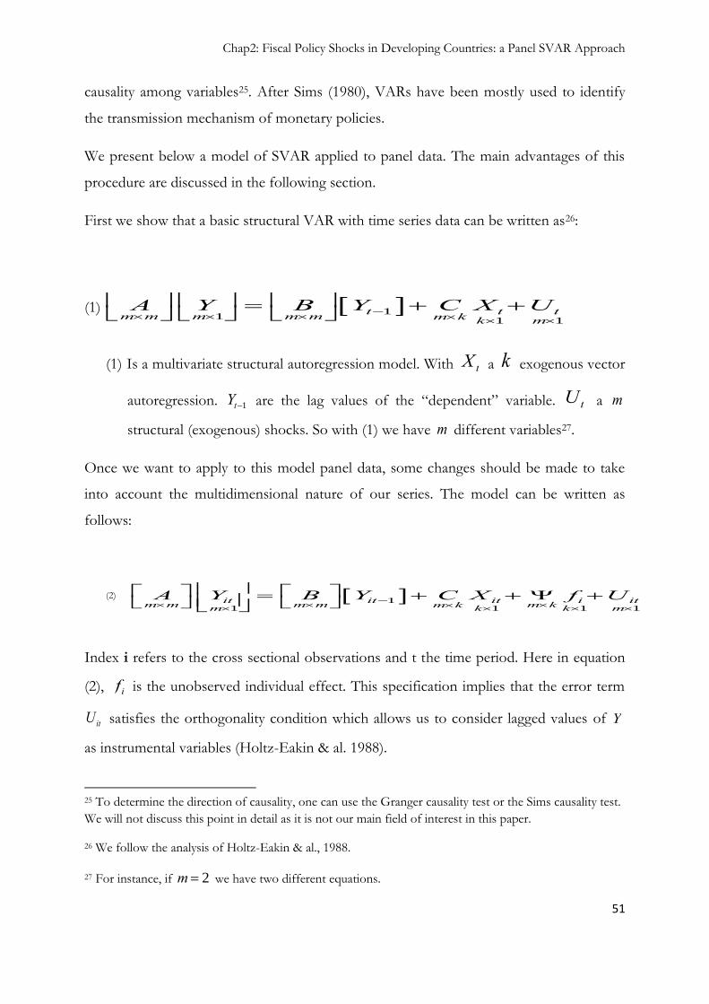
Chap2: Fiscal Policy Shocks in Developing Countries: a Panel SVAR Approach
51
causality among variables25. After Sims (1980), VARs have been mostly used to identify
the transmission mechanism of monetary policies.
We present below a model of SVAR applied to panel data. The main advantages of this
procedure are discussed in the following section.
First we show that a basic structural VAR with time series data can be written as26:
(1) 11
1 1t t tm m m m m m k k m
A Y B Y C X U
(1) Is a multivariate structural autoregression model. With tX a k exogenous vector
autoregression. 1tY are the lag values of the “dependent” variable. tU a m
structural (exogenous) shocks. So with (1) we have m different variables27.
Once we want to apply to this model panel data, some changes should be made to take
into account the multidimensional nature of our series. The model can be written as
follows:
(2) 11 1 1 1
it it it i itm m m m m km km k k mA Y B Y C X f U
Index i refers to the cross sectional observations and t the time period. Here in equation
(2), if is the unobserved individual effect. This specification implies that the error term
itU satisfies the orthogonality condition which allows us to consider lagged values of Y
as instrumental variables (Holtz-Eakin & al. 1988).
25 To determine the direction of causality, one can use the Granger causality test or the Sims causality test.
We will not discuss this point in detail as it is not our main field of interest in this paper.
26 We follow the analysis of Holtz-Eakin & al., 1988.
27 For instance, if 2m we have two different equations.

Chap2: Fiscal Policy Shocks in Developing Countries: a Panel SVAR Approach
52
The main advantage of introducing the individual effect is that it allows us to consider
that the time series relationship between the dependent variables, its lag values and the
exogenous variables is not identical (Holtz-Eakin & al. 1988). In equation (2) we also
allow the variance of U (the structural innovation) to differ with the cross-section unit
(that‟s why U is indexed with i).
According to Holtz-Eakin & al. (1988), using SVARs with panel data has the advantage of
allowing us to relax the assumption of time stationarity, as the presence of a large number
of cross-sectional units makes it possible for lag coefficient to vary over time.
In this model, though we want to estimate the coefficients A , B and U , the issue is that
one can only observe a statistical VAR (reduced-form VAR):
(3) 1it it it itY VY WX e
With ite is a vector of statistical innovations (a reduced-form residual and not a structural
shock) which are a combination of the structural innovations ( itU ). The main question is
how to recover the “missing” coefficient from V and e . To do so, one can write:
11 1 1
11
1
it it it it
it it it it
it t
AY BY CX UY A BY A CX A UV A B
e A U
The variance of ite is: 21var( ) var( )it ite A U .
The assumption that the structural innovations are uncorrelated across time and between
individuals means that the matrix of the variance of those structural shocks is a diagonal.
1 0var( )
0 1itU I
1 0 1 0
U I U I U IU I U IU I U IU I U I U I U I U I U IU I U I U I U I
0 1 0 1 0 1 0 1 0 1 0 1 0 1 0 1

Chap2: Fiscal Policy Shocks in Developing Countries: a Panel SVAR Approach
53
The orthogonality condition presented above also holds for the structural innovation on
the panel model28.
And the variance of the reduced-form residual ite is a symmetric matrix:
var( )ij
it
ji
ae
a
ij ija a
ij
ij ij ij
ij ija a
a a
ij
ij
var( )ite is a m m matrix; with ij jia a
Then we have: 1
var itA e
So from this matrix one can recover 21
2m
m
coefficients. Whereas we need to
estimate 2m coefficients of A (to retrieve A ) but we only have 21
2m
m
of estimates
available from var( )ite .
To solve this problem we need some restriction on matrix A as Blanchard & Perotti
(2002), or use the Cholesky decomposition.
In this study we will use both methods to estimate the impulse responses from our SVAR
in order to have a situation of reference and benchmark estimation.
2.3.3 Identification methods: Blanchard & Perotti and Cholesky ordering
Before presenting our data and the sample used in this paper, explanations will be
given on the two different identification methods: the Blanchard & Perotti technique and
the Cholesky decomposition method.
28
This condition is that : 0it it it itY U X U

Chap2: Fiscal Policy Shocks in Developing Countries: a Panel SVAR Approach
54
2.3.3.1 Blanchard & Perotti identification method:
First Blanchard & Perotti (2002) write down the reduced form residuals (of the three
different VARs they are using) as a linear combination of the underlying structural
innovation. Then, they rely on institutional information (and on other studies) to estimate
the impact of unexpected movements of GDP on taxes and government spending. To do
this they construct the elasticities to output of public spending and government revenue.
The estimation of those coefficients will allow them to construct the cyclically adjusted
reduced form of their variables of interest (taxes and spending). As the cyclically adjusted
reduced form of tax and spending are not correlated to the structural shocks we can use
them as instruments to estimate the impact of unexpected movement of taxes and
spending on output. The remaining problem to solve here will be the estimation of the
impact of the unexpected changes of taxes (spending) on spending (government revenue).
To solve the problem they do not consider the two decisions at the same time. For
instance, the decision of increasing the expenses can be considered as coming first and
one is able to estimate the impact of unexpected change of spending on taxes29.
In more detail, by using matrices the SVAR specification is as follow:
24 21 23
34 31 32
42 43 41
1 0 0 0 1 0 0 0
0 1 0 1 0
0 0 1 1 0
0 1 0 0 1
govspen govspent tgovreve govrevet tpriconso priconso
t ty yt t
u vu vu v
u v
(4)
Here I will use only some variables to illustrate the Blanchard & Perotti identification
method. The full set of variables is presented in the empirical section of the chapter. The
vector of variables tX = t t t tgovspen , govreve , priconso , y represents
29 However as authors said, we believe that the ordering does not make big differences in the results as
there is little correlation between the cyclically adjusted reduced form of taxes and spending.

Chap2: Fiscal Policy Shocks in Developing Countries: a Panel SVAR Approach
55
government spending, government revenues, private consumption and GDP. tv is the
matrix of structural shocks, and the right hand side coefficients capture the automatic
stabilizers effects (Kumah & Matovu, 2007) and as said earlier this matrix is uncorrelated
with a diagonal contemporaneous covariance matrix , tu is a matrix of innovations.
The coefficients of the left-hand side (the tu ) capture the stochastic effects (automatic
stabilizers) and the right-hand side coefficients (the tv ) represent the effects of
discretionary policies (policy shocks).
Therefore the issue here will consist of identifying discretionary shocks (from automatic
responses of fiscal variables to change in economic activity). For Blanchard & Perotti
(Kumah & Matovu, 2007 used the same approach), using quarterly data ensures that there
is no reaction of fiscal variables due to an automatic stabilizers effect. Therefore within a
quarter a change in any fiscal variable is due to a voluntary action from policy makers. In
addition, the structure of the model allows us to introduce clear constraints that refrain
other variables (in case they could influence fiscal aggregates within a quarter) from
influencing the public finances stance.
31 32
41 42
1 0 0 0
0 1 0 0
1 0
0 1
govspen govspent tgovreve govrevet tpriconso priconso
t ty yt t
u vu vu v
u v
(5)
The final form of the system is presented in equation (5). Government spending and
public revenue shocks are strictly exogenous30. Coefficients 31 and 32 show the
response of price level to government spending shocks and public revenue shocks. While
42 and 41 represent the effects on output of shocks on fiscal variables.
30 Here it is possible to consider that government revenues can respond to discretionary change in public
expenditure. In such situations, the coefficient (second raw, fourth column) will be different from zero.

Chap2: Fiscal Policy Shocks in Developing Countries: a Panel SVAR Approach
56
2.3.3.2 The Cholesky ordering
Cholesky ordering is a statistical decomposition of symmetric positive-definite matrix.
This procedure allows us to orthogonalise the residuals using the inverse of the Cholesky
factor of the residual covariance matrix. This procedure is simple as one does not need to
write a matrix and impose restrictions (Younus, 2005). But it is quite risky when the
ordering of the variables in the VAR is vital as it attributes all of the effects of any
common component to the variable that comes first in the VAR system. Once we change
the ordering we obtain different results.
In the estimations, I will use both methods and see which one gives the most interesting
empirical explanations of the phenomenon studied in this chapter.
2.4 The data and estimations
This section gives a brief presentation of the data, and presents the empirical results.
The list of countries is shown in appendix.
We use quarterly panel data in our estimations. The use of quarterly data is mainly
justified by our objective to identify the outcomes of fiscal policy shocks. If annual
instead of quarterly data was used, there might be loss of information. This is simply due
to the fact that shocks happening in the first months of the year can be completely
smoothed at the end of the year. Besides, in a quarter, a change in fiscal variables is only
due to fiscal policy shocks and not the economic activity. In other words it takes more
than one quarter for fiscal variables to react to variation in the economic activity
(Blanchard & Perotti, 2002). This assumption justifies basically the restriction I make on
the structural residuals.
The long period of observation in our data (1960 to early 2002) gives us the opportunity
to take into account many changes in fiscal policy that have taken place in developing
countries (debt crisis for some, raw materials shocks, etc.). Moreover this deep temporal
dimension is necessary to obtain enough instrumental variables to identify the system as

Chap2: Fiscal Policy Shocks in Developing Countries: a Panel SVAR Approach
57
this is necessary to estimate (according to the number of VARs in our model) an
important number of coefficients.
2.4.1 The data and summary statistics
One uses the International Financial Statistics (IFS) data base of the International
Monetary Fund (IMF). As said above the data covers the period from 1960 to 2002. All
variables are in percent of GDP (consumer price index used as deflator) and put in log
form (except the real effective exchange rate).
The main series are general government spending and revenues, private consumption,
trade account balance, and real GDP per capita, all from the IFS data base. In what
follows, an increase in the real effective exchange rate (REER) reflects an appreciation
and therefore a loss of competitiveness. A full definition of the variables is presented in
annex.
Like many others, this study faces the problem of availability of data especially with
regard to quarterly data. Despite this issue, the frequency and the length of the data end
up being an advantage since it gives enough observation and variability allowing us to run
the estimations.
I use data from a sample of 34 developing countries. Table 2.1 gives some summary
statistics.
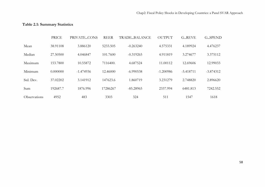
Chap2: Fiscal Policy Shocks in Developing Countries: a Panel SVAR Approach
58
Table 2.1: Summary Statistics
PRICE
PRIVATE_CONS
REER
TRADE_BALANCE
OUTPUT
G_REVE
G_SPEND
Mean 38.91108 3.886120 5233.505 -0.263240 4.575331 4.189924 4.476237 Median 27.50500 4.046847 101.7600 -0.319265 4.911819 3.274677 3.375112 Maximum 153.7800 10.55872 7116400. 4.687524 11.00112 12.69606 12.99033 Minimum 0.000000 -1.474936 12.46000 -6.990538 -1.200986 -5.418711 -3.874312 Std. Dev. 37.02202 3.141912 147623.6 1.860719 3.231279 2.748820 2.896620
Sum 192687.7 1876.996 17286267 -85.28965 2337.994 6481.813 7242.552
Observations 4952 483 3303 324 511 1547 1618
Chap2: Fiscal Policy Shocks in Developing Countries: a Panel SVAR Approach
59
2.4.2 The empirical results
The main concern while running the impulse responses on panel data was a possible
correlation between residuals across countries. But Ravn & al., (2006) show that this
problem is very negligible and results do not change if one applies GLS estimation31.
Formally, following Blanchard & Perotti‟s identification method, I consider that within a
quarter, government spending (or government revenue) only respond to innovations to
government spending. Then I just impose the first row of matrix A to be equal to 1 for its
first element and zero elsewhere. After that, I present in this section the impact of a fiscal
policy shock on output, private consumption, real effective exchange rate and trade
balance. To avoid having an important number of coefficients to estimate and therefore
the loss of a degree of freedom, I do not introduce all variables of interest in the same
VAR. Only a maximum of five variables are therefore considered in one SVAR
specification to sort out this problem.
I first present the results from a structural decomposition using the Blanchard & Perotti
(2002) method and use the Cholesky decomposition as a benchmark to our findings.
2.4.2.1 Responses to a government spending shock
Statistically significant estimations are those for which the two standard error bands
do not include the zero line. In other words as soon as the zero line is between the
standards error bands this would mean that the impulse response is not statistically
significant, and hence the variable considered is not responding to the shock32. Another
particular aspect of SVAR is that since it is a forecasting tool showing outcomes after a
sudden change in policy, then there is not a single coefficient estimated. The model only
31 Generalized Least Squares (used when OLS is inconsistent) is an estimation method used when there is
some heteroscedasticity or a correlation between the observations.
32 Mountford & Uhlig, (2005) used the same method to interpret their results.
Chap2: Fiscal Policy Shocks in Developing Countries: a Panel SVAR Approach
60
estimates the coefficients inside the matrix which will be used to determine impulse
responses.
I consider that the government purchases increase suddenly and this situation is
unexpected. Figure 2.1 displays the impact from a structural decomposition.
As we see, the shock on government spending itself is persistent. The impact on GDP is
quasi simultaneous, positive and lasts relatively long. The private agents, unexpecting the
fiscal policy increase their consumption probably due to a wealth effect. The effect on
trade balance is negative but not very significant. Obviously, this shows us that after the
shock, the country seems to increase its importation and that this situation is transitory as
after five to seven quarters the effects of the fiscal policy on the trade balance disappear.
These results, which will later be compared to other findings, remain strong even when
the Cholesky decomposition is used (Figure 2.2).
In Figure A.2.1 (Appendix1), only the real effective exchange rate is added and the trade
balance taken out as we avoid an important loss in the degree of freedom. The same
effects are found with slight differences. The government spending shock seems to be
persistent. For output and private consumption, the response comes with a small lag of
less than six month but it remains that the effect on those variables is positive and
persistent. Unfortunately, the real effective exchange rate (REER) does not respond
significantly to a spending shock even when one uses a different identification method
like the Cholesky decomposition (Figure A.2.2, Appendix1).
2.4.2.2 Impulse response to a government revenue shock
Impulse responses to a government revenue shock are presented in Figures 2.3 & 2.4.
The sudden increase of government revenue is quite persistent and also has an impact on
government purchases that increase at the same time. It can be surprising to see that a
public revenue shock has a positive impact on output and on household consumption.
These results are at odds with Blanchard & Perotti (2002) results for the US economy.
Some ideas will be brought to try to explain these “uncommon” results for developing

Chap2: Fiscal Policy Shocks in Developing Countries: a Panel SVAR Approach
61
countries. When one has a look at the external sector, we first see that REER do not
respond to a revenue shock (Figures A.2.3 & A.2.4, Appendix2). The trade balance
deteriorates but the shock seems to be transitory. Most of our results for this sample of
developing countries are quite original. But as said above one cannot perform a
comparison as no other study on panel SVAR is applied to developing countries to
identify fiscal shocks. Nevertheless in the coming section, and relying on what is known
of the economic environment of developing countries, some interpretations will be given.
Figure 2.1: Impulse response from government spending shock
.05
.10
.15
.20
.25
.30
1 2 3 4 5 6 7 8 9 10
Response of G_SPEND to Shock1
.00
.04
.08
.12
.16
.20
.24
1 2 3 4 5 6 7 8 9 10
Response of OUTPUT to Shock1
.00
.05
.10
.15
.20
.25
1 2 3 4 5 6 7 8 9 10
Response of PRIVATE_CONS to Shock1
-.8
-.6
-.4
-.2
.0
.2
1 2 3 4 5 6 7 8 9 10
Response of TRADE_BALANCE to Shock1
.05
.10
.15
.20
.25
.30
1 2 3 4 5 6 7 8 9 10
Response of G_REVE to Shock1
Response to Structural One S.D. Innovations ± 2 S.E.
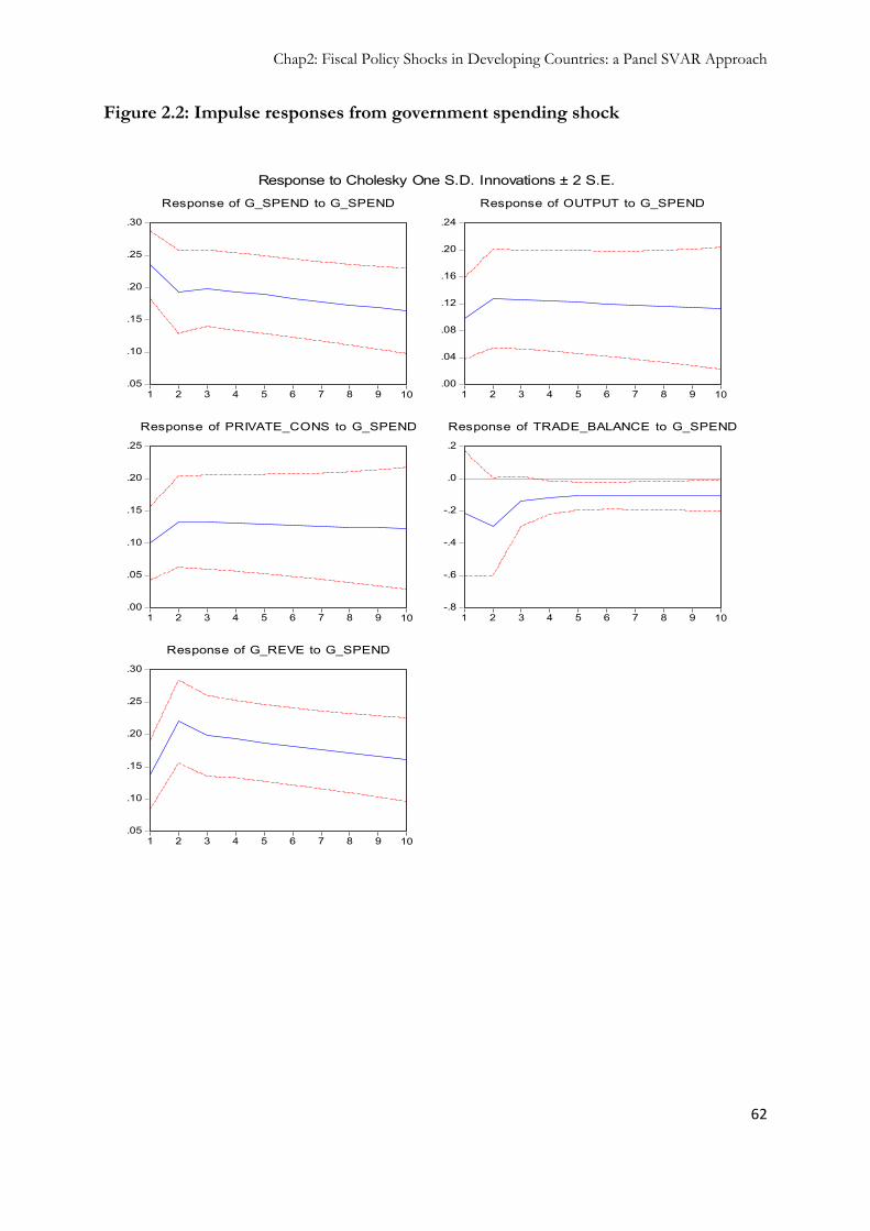
Chap2: Fiscal Policy Shocks in Developing Countries: a Panel SVAR Approach
62
Figure 2.2: Impulse responses from government spending shock
.05
.10
.15
.20
.25
.30
1 2 3 4 5 6 7 8 9 10
Response of G_SPEND to G_SPEND
.00
.04
.08
.12
.16
.20
.24
1 2 3 4 5 6 7 8 9 10
Response of OUTPUT to G_SPEND
.00
.05
.10
.15
.20
.25
1 2 3 4 5 6 7 8 9 10
Response of PRIVATE_CONS to G_SPEND
-.8
-.6
-.4
-.2
.0
.2
1 2 3 4 5 6 7 8 9 10
Response of TRADE_BALANCE to G_SPEND
.05
.10
.15
.20
.25
.30
1 2 3 4 5 6 7 8 9 10
Response of G_REVE to G_SPEND
Response to Cholesky One S.D. Innovations ± 2 S.E.
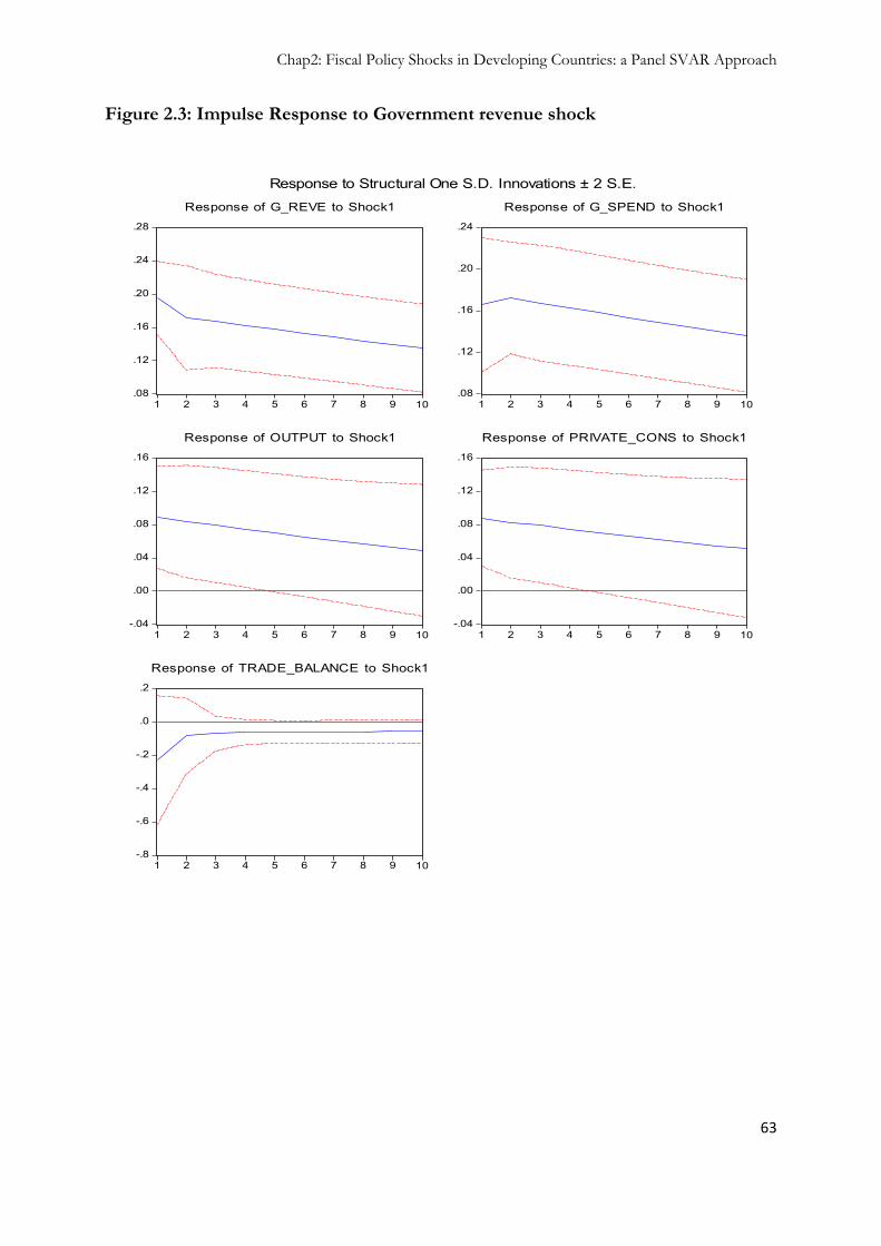
Chap2: Fiscal Policy Shocks in Developing Countries: a Panel SVAR Approach
63
Figure 2.3: Impulse Response to Government revenue shock
.08
.12
.16
.20
.24
.28
1 2 3 4 5 6 7 8 9 10
Response of G_REVE to Shock1
.08
.12
.16
.20
.24
1 2 3 4 5 6 7 8 9 10
Response of G_SPEND to Shock1
-.04
.00
.04
.08
.12
.16
1 2 3 4 5 6 7 8 9 10
Response of OUTPUT to Shock1
-.04
.00
.04
.08
.12
.16
1 2 3 4 5 6 7 8 9 10
Response of PRIVATE_CONS to Shock1
-.8
-.6
-.4
-.2
.0
.2
1 2 3 4 5 6 7 8 9 10
Response of TRADE_BALANCE to Shock1
Response to Structural One S.D. Innovations ± 2 S.E.

Chap2: Fiscal Policy Shocks in Developing Countries: a Panel SVAR Approach
64
Figure 2.4: Impulse Response to Government revenue shock
.08
.12
.16
.20
.24
.28
1 2 3 4 5 6 7 8 9 10
Response of G_REVE to G_REVE
.08
.12
.16
.20
.24
1 2 3 4 5 6 7 8 9 10
Response of G_SPEND to G_REVE
-.04
.00
.04
.08
.12
.16
1 2 3 4 5 6 7 8 9 10
Response of OUTPUT to G_REVE
-.04
.00
.04
.08
.12
.16
1 2 3 4 5 6 7 8 9 10
Response of PRIVATE_CONS to G_REVE
-.8
-.6
-.4
-.2
.0
.2
1 2 3 4 5 6 7 8 9 10
Response of TRADE_BALANCE to G_REVE
Response to Cholesky One S.D. Innovations ± 2 S.E.

Chap2: Fiscal Policy Shocks in Developing Countries: a Panel SVAR Approach
65
2.4.3 The Stationarity Issue
Given the length of the period of observation (more than 150 quarters) some series
can be deemed as non-stationary. However another view states that this issue is not a
major concern in panel SVARs and (many) other studies ignore the possible existence of a
unit root. For instance, Ravn & al. 2007, Montford & Uhlig 2005 consider that their
quarterly series has no unit root during the period 1955-2000. This assumption (not
considering the existence of unit root in such data) for series like price, trade balance and
output seems a bit hard to defend. In what follows, one tries to address this issue by
running several panel unit root tests.
Apart from the usual panel unit root tests (details on such tests are provided later in this
paragraph), VEC models (Vector Error Correction Model) can be used to sort out the
non-stationarity. The VEC model is a restricted VAR designed for use with non-
stationary series that are known to be cointegrated. Indeed, once the econometrical tests
show that variables are non-stationary and if there exists some cointegration, then VEC
procedure becomes robust. Despite such advantages the VEC model presents some
limits. Indeed with VEC procedure, structural shocks with transitory effects do not have
contemporaneous effect on weak exogenous variables (Fisher & Huh, 1999). In addition,
VECs can only be used with unrestricted VARs, and are therefore not consistent with the
main purpose of this chapter. Given these important limits, the VEC model will not be
used.
Hence our method will consist of testing for the stationarity of each variable and once a
variable has a unit root the first difference will be used in the estimations. The results
indicate that (see Appendix5) private consumption, government spending, price level and
output growth are non-stationary, while other variables (government revenue, trade
balance and exchange rate seem more stationary). The next step is to use first differences
instead of the simple log of variables. Then the same shocks are introduced with new
variables, as previously.

Chap2: Fiscal Policy Shocks in Developing Countries: a Panel SVAR Approach
66
Once first differences are considered, the immediate effect after the shock is roughly
identical to previous results. Appendix 6 FigureA.2.5 shows that a spending shock does
not affect the external sector (trade balance)33. As previously, public spending
discretionary increase receives a positive impulse response from private consumption,
output and government revenue. However a major change is noticed on the durability of
the responses of the variables of interest. Indeed, discretionary measures on public
spending disappear after only 2 quarters (while in the previous paragraph the change was
quasi-permanent). Impulse responses from output and private consumption also
disappear after 3 to 4 quarters. The fact that the response to shocks disappears more
rapidly than previously (situation where series were non-stationary) demonstrates that the
series was highly non-stationary and this affected the results. Impulse responses after a
government revenue shock are presented in Appendix6 FigureA.2.7 & FigureA.2.8. Here
again no major change in the results except for the durability of the impact of shocks.
The last puzzle remains the response of government revenues to public expenditures
shock that remain unchanged for a relative long period (more than 9 quarters). Also
usually discretionary changes in government revenue last quite longer. For developing
countries, since automatic stabilizers are weak (Carmignani, 2010) due to small
government size, public revenues do not readapt quickly to change in economic activity34.
Indeed this denotes rigidity, especially on the revenue side since policy makers are not
able to change tax rates after the period of resilience of real economy following a shock.
2.5 Discussion and Policy Recommendations
The impulse responses to a government spending shock in developing countries are
similar to those found in advanced economies. Indeed the main studies find a positive
effect of an unexpected increase in spending on output and private consumption
33 The result is similar when REER is considered instead of trade balance.
34 In most African countries, the substantial ineffectiveness of formal social safety networks implies that automatic stabilizers are weak (Carmignani, 2010).

Chap2: Fiscal Policy Shocks in Developing Countries: a Panel SVAR Approach
67
(Blanchard & Perotti 2002; Giordano & al. 2007 and Ravn & al., 2007). According to
Giordano & al. (2007) the positive impact on government revenue of a spending shock is
due to the increase in wages that enhances tax revenue. This result can hold for
developing countries once one knows that the public sector is a major actor (in many
instances, government is the first employer) in these economies. Nevertheless the effect
on output for developing countries works differently from what was found previously in
the literature. That is in some cases when the data provides the opportunity to see which
part of public spending, after a rise in government expenditures. This is simply due to the
fact that when government purchases increase the public revenue remains the same (or
decreases) and this facilitates the rise of economic activity. For developing countries (even
if we do not test this hypothesis due to the scarcity of quarterly data), when the
government suddenly increases its expenses, public revenue and output increase. This is
not a surprising result as government is the major actor in developing economies and
most of investments are public. Therefore it is understandable that the GDP increases.
Concerning the external sector, our findings are in line with the results in the literature.
Funke & Nickel (2006) find that an increase in government expenditures has a positive
impact on both import of goods and services. This leads to a deterioration of the trade
account. The same mechanism works in our analysis (even if our results are not highly
significant) in the sense that consumption needs for the public sector after a shock are so
important that imports should increase. However we still don‟t have the exact impact of
government spending shock on the competitiveness of developing countries. This will be
understood after I make clear the impact of a shock on trade balance. The first
explanation could be the quality of our data when we see how scarce quarterly data can
be. Another explanation for this outcome can be that the developing countries import
most of their consumption during shocks or in normal times. Therefore the situation
does not change that much after a shock in the sense that the country is not shifting from
a state of net exporter to a net importer (only imports increase so there is not any
important variability).
The impulse responses to a government revenue shock can be seen as counter-intuitive.
We find a positive response of GDP and private consumption to a government revenue

Chap2: Fiscal Policy Shocks in Developing Countries: a Panel SVAR Approach
68
shock. Blanchard & Perotti (2002) as said above found different results that are more
close to the Keynesian predictions. In the context of developing economies, positive
effects on government spending are understandable. As previously said, in these
economies, the government is the main investor and in many situations it is the first
employer35. So once the revenue increases the expenses go the same way. Another
argument to this could be the idea of “starving the leviathan”. This argument was used to
explain why fiscal policy is procyclical in developing countries. Indeed, when the
economy is doing well, and the government is getting more revenue, the voters do not
want the government to appropriate the rent so they ask for more public goods or higher
wages (Alesina & Tabellini, 2005). Aware of that, the government increases its expenses
after a revenue shock since it anticipate the political pressure from citizens. A government
revenue shock has a small effect on the external sector and only the trade account
deteriorates (the impulse response on REER remaining not statistically significant). The
explanation is that the government can afford more goods and services from abroad after
the shock and it is obliged to do so by its citizens in accordance with the “starving
leviathan” idea already seen.
According to Favero & Giavazzi (2007) the impulse response estimated in VAR studies
of fiscal policy shocks are all biased. The reason for this is that these studies do not
consider the debt dynamics that arise after a fiscal policy shock. In other words, the
response of tax and spending after a fiscal shock depends on the path the government has
chosen to meet its intertemporal budget constraint and this depends on the level of public
debt. Nevertheless this critique does not mean that the traditional VAR findings should
be sent to the bin as only the very short run effects are indentified by this approach. The
intertemporal budget constraint has to be met evidently, but as the shock is unanticipated
(in this SVAR studies), in the short run private agents only focus on the “shock”.
35 Giordano & al. 2007 find the same “surprising” results to a government revenue shock.
Chap2: Fiscal Policy Shocks in Developing Countries: a Panel SVAR Approach
69
2.6 Conclusions
After summing up our findings, one can see that in some way fiscal policy shocks
have a different effect in developing countries compared to their industrial counterparts.
Though the effects of a government spending shock can be positive for a developing
economy in the sense that it brings growth and induces more consumption on the one
hand, the effects seem to be the same after government revenue shock on the other. But
the second aspect of these results means that there is a weak (or a less strong) private
sector in the developing world. Compared to previous studies, this one addresses the
important issue of non-stationarity of series. The numerous tests implemented have
shown that some series were non-stationary. Once this issue is corrected, a noticeable
change arises: impulse responses are shorter, the effect of the shock disappearing after
four quarters on average. However due to weak automatic stabilizers in developing
countries, impulse response of government revenues (even if series are purged from unit
roots) was persistent.
For policy makers a possible response regarding the effects of revenue shocks could be
the adoption of more transparent budgetary processes. Implementing a fiscal rule might
add some discipline and afford some credibility to fiscal authorities. Weak automatic
stabilisers, with the possible consequence of increasing procyclicality of fiscal policies,
could be addressed with a larger government size (a long term process).
This study fills an important gap since such analysis has not been done yet for middle and
low income countries. Despite the diversity of economic structures for countries in the
sample, the analysis did not suffer much of that since SVARs are robust sample
heterogeneity and the unit root test in a sense removes some inconsistencies in the results.
Future analysis may focus on ways and means to improve the credibility of fiscal
authorities. As the third chapter in this dissertation will demonstrate, developing
countries‟ main cause of fiscal policy inefficiency is due to the poor confidence of tax
payers on public authorities.

Chap2: Fiscal Policy Shocks in Developing Countries: a Panel SVAR Approach
70
Annexes Chapter 2

Chap2: Fiscal Policy Shocks in Developing Countries: a Panel SVAR Approach
71
APPENDIX 1
Figure A.2.1: Impulse responses to Government spending shock (Structural ordering)
.12
.16
.20
.24
.28
.32
1 2 3 4 5 6 7 8 9 10
Response of G_SPEND to Shock1
.12
.16
.20
.24
.28
1 2 3 4 5 6 7 8 9 10
Response of G_REVE to Shock1
.08
.12
.16
.20
.24
.28
1 2 3 4 5 6 7 8 9 10
Response of OUTPUT to Shock1
.08
.12
.16
.20
.24
.28
1 2 3 4 5 6 7 8 9 10
Response of PRIVATE_CONS to Shock1
-3
-2
-1
0
1 2 3 4 5 6 7 8 9 10
Response of REER to Shock1
Response to Structural One S.D. Innovations ± 2 S.E.
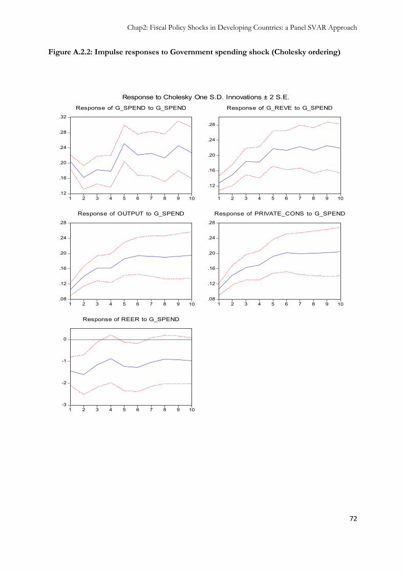
Chap2: Fiscal Policy Shocks in Developing Countries: a Panel SVAR Approach
72
Figure A.2.2: Impulse responses to Government spending shock (Cholesky ordering)
.12
.16
.20
.24
.28
.32
1 2 3 4 5 6 7 8 9 10
Response of G_SPEND to G_SPEND
.12
.16
.20
.24
.28
1 2 3 4 5 6 7 8 9 10
Response of G_REVE to G_SPEND
.08
.12
.16
.20
.24
.28
1 2 3 4 5 6 7 8 9 10
Response of OUTPUT to G_SPEND
.08
.12
.16
.20
.24
.28
1 2 3 4 5 6 7 8 9 10
Response of PRIVATE_CONS to G_SPEND
-3
-2
-1
0
1 2 3 4 5 6 7 8 9 10
Response of REER to G_SPEND
Response to Cholesky One S.D. Innovations ± 2 S.E.
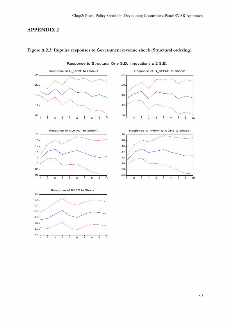
Chap2: Fiscal Policy Shocks in Developing Countries: a Panel SVAR Approach
73
APPENDIX 2
Figure A.2.3: Impulse responses to Government revenue shock (Structural ordering)
.08
.12
.16
.20
.24
1 2 3 4 5 6 7 8 9 10
Response of G_REVE to Shock1
.08
.12
.16
.20
.24
1 2 3 4 5 6 7 8 9 10
Response of G_SPEND to Shock1
.06
.08
.10
.12
.14
.16
.18
.20
1 2 3 4 5 6 7 8 9 10
Response of OUTPUT to Shock1
.06
.08
.10
.12
.14
.16
.18
.20
1 2 3 4 5 6 7 8 9 10
Response of PRIVATE_CONS to Shock1
-2.5
-2.0
-1.5
-1.0
-0.5
0.0
0.5
1.0
1 2 3 4 5 6 7 8 9 10
Response of REER to Shock1
Response to Structural One S.D. Innovations ± 2 S.E.

Chap2: Fiscal Policy Shocks in Developing Countries: a Panel SVAR Approach
74
Figure A.2.4: Impulse responses to Government revenue shock (Cholesky ordering)
.08
.12
.16
.20
.24
1 2 3 4 5 6 7 8 9 10
Response of G_REVE to G_REVE
.08
.12
.16
.20
.24
1 2 3 4 5 6 7 8 9 10
Response of G_SPEND to G_REVE
.04
.08
.12
.16
.20
1 2 3 4 5 6 7 8 9 10
Response of OUTPUT to G_REVE
.04
.08
.12
.16
.20
1 2 3 4 5 6 7 8 9 10
Response of PRIVATE_CONS to G_REVE
-2
-1
0
1
1 2 3 4 5 6 7 8 9 10
Response of REER to G_REVE
Response to Cholesky One S.D. Innovations ± 2 S.E.
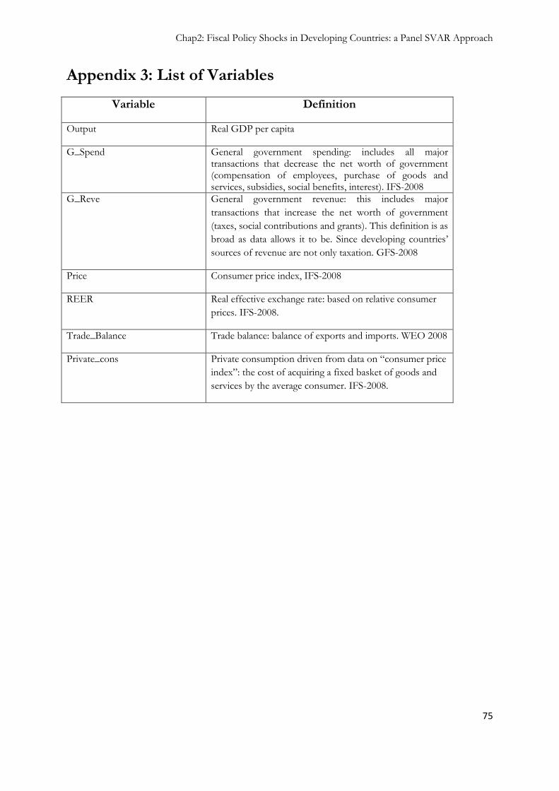
Chap2: Fiscal Policy Shocks in Developing Countries: a Panel SVAR Approach
75
Appendix 3: List of Variables
Variable Definition
Output Real GDP per capita
G_Spend General government spending: includes all major transactions that decrease the net worth of government (compensation of employees, purchase of goods and services, subsidies, social benefits, interest). IFS-2008
G_Reve General government revenue: this includes major
transactions that increase the net worth of government
(taxes, social contributions and grants). This definition is as
broad as data allows it to be. Since developing countries‟
sources of revenue are not only taxation. GFS-2008
Price Consumer price index, IFS-2008
REER Real effective exchange rate: based on relative consumer
prices. IFS-2008.
Trade_Balance Trade balance: balance of exports and imports. WEO 2008
Private_cons Private consumption driven from data on “consumer price
index”: the cost of acquiring a fixed basket of goods and
services by the average consumer. IFS-2008.
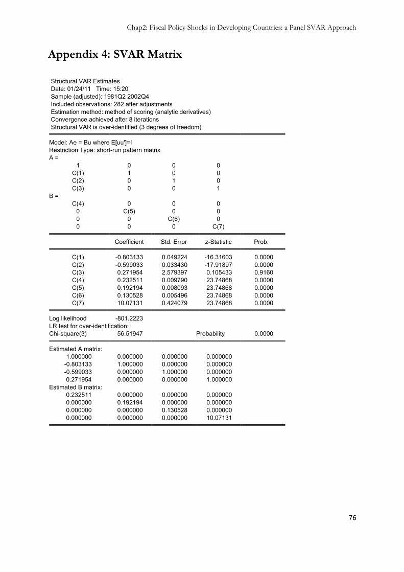
Chap2: Fiscal Policy Shocks in Developing Countries: a Panel SVAR Approach
76
Appendix 4: SVAR Matrix
Structural VAR Estimates Date: 01/24/11 Time: 15:20 Sample (adjusted): 1981Q2 2002Q4 Included observations: 282 after adjustments Estimation method: method of scoring (analytic derivatives) Convergence achieved after 8 iterations Structural VAR is over-identified (3 degrees of freedom)
Model: Ae = Bu where E[uu']=I
Restriction Type: short-run pattern matrix A =
1 0 0 0 C(1) 1 0 0 C(2) 0 1 0 C(3) 0 0 1
B = C(4) 0 0 0
0 C(5) 0 0 0 0 C(6) 0 0 0 0 C(7) Coefficient Std. Error z-Statistic Prob. C(1) -0.803133 0.049224 -16.31603 0.0000
C(2) -0.599033 0.033430 -17.91897 0.0000 C(3) 0.271954 2.579397 0.105433 0.9160 C(4) 0.232511 0.009790 23.74868 0.0000 C(5) 0.192194 0.008093 23.74868 0.0000 C(6) 0.130528 0.005496 23.74868 0.0000 C(7) 10.07131 0.424079 23.74868 0.0000
Log likelihood -801.2223
LR test for over-identification: Chi-square(3) 56.51947 Probability 0.0000
Estimated A matrix:
1.000000 0.000000 0.000000 0.000000 -0.803133 1.000000 0.000000 0.000000 -0.599033 0.000000 1.000000 0.000000 0.271954 0.000000 0.000000 1.000000
Estimated B matrix: 0.232511 0.000000 0.000000 0.000000 0.000000 0.192194 0.000000 0.000000 0.000000 0.000000 0.130528 0.000000 0.000000 0.000000 0.000000 10.07131

Chap2: Fiscal Policy Shocks in Developing Countries: a Panel SVAR Approach
77
Appendix 5: Panel Unit Root Test
Table 1
Panel unit root test: Summary Series: Private Consumption Date: 01/18/11 Time: 17:24 Sample: 1960Q1 2002Q4 Exogenous variables: Individual effects Automatic selection of maximum lags Automatic selection of lags based on SIC: 0 to 7 Newey-West bandwidth selection using Bartlett kernel Cross- Method Statistic Prob.** sections Obs Null: Unit root (assumes common unit root process) Levin, Lin & Chu t* -0.42597 0.3351 10 429
Null: Unit root (assumes individual unit root process) Im, Pesaran and Shin W-stat 5.11188 1.0000 10 429 ADF - Fisher Chi-square 13.5207 0.8539 10 429 PP - Fisher Chi-square 8.40285 0.9888 10 456 ** Probabilities for Fisher tests are computed using an asymptotic Chi -square distribution. All other tests assume asymptotic normality.
Table 2
Panel unit root test: Summary Series: Government Spending Date: 01/18/11 Time: 20:48 Sample: 1960Q1 2002Q4 Exogenous variables: Individual effects Automatic selection of maximum lags Automatic selection of lags based on SIC: 0 to 8 Newey-West bandwidth selection using Bartlett kernel Cross- Method Statistic Prob.** sections Obs Null: Unit root (assumes common unit root process) Levin, Lin & Chu t* 6.09230 1.0000 24 1495
Null: Unit root (assumes individual unit root process) Im, Pesaran and Shin W-stat 7.44552 1.0000 23 1492 ADF - Fisher Chi-square 37.9217 0.8512 24 1495 PP - Fisher Chi-square 146.786 0.0000 24 1577 ** Probabilities for Fisher tests are computed using an asymptotic Chi -square distribution. All other tests assume asymptotic normality.

Chap2: Fiscal Policy Shocks in Developing Countries: a Panel SVAR Approach
78
Table 3
Panel unit root test: Summary Series: PRICE Date: 01/18/11 Time: 20:40 Sample: 1960Q1 2002Q4 Exogenous variables: Individual effects Automatic selection of maximum lags Automatic selection of lags based on SIC: 0 to 12 Newey-West bandwidth selection using Bartlett kernel Cross- Method Statistic Prob.** sections Obs Null: Unit root (assumes common unit root process) Levin, Lin & Chu t* 12.0889 1.0000 34 4749
Null: Unit root (assumes individual unit root process) Im, Pesaran and Shin W-stat 17.6911 1.0000 34 4749 ADF - Fisher Chi-square 15.6799 1.0000 34 4749 PP - Fisher Chi-square 8.85315 1.0000 34 4913 ** Probabilities for Fisher tests are computed using an asymptotic Chi -square distribution. All other tests assume asymptotic normality.
Table 4
Panel unit root test: Summary Series: OUTPUT Date: 01/18/11 Time: 20:40 Sample: 1960Q1 2002Q4 Exogenous variables: Individual effects Automatic selection of maximum lags Automatic selection of lags based on SIC: 0 to 7 Newey-West bandwidth selection using Bartlett kernel Cross- Method Statistic Prob.** sections Obs Null: Unit root (assumes common unit root process) Levin, Lin & Chu t* -0.03618 0.4856 11 457
Null: Unit root (assumes individual unit root process) Im, Pesaran and Shin W-stat 6.20757 1.0000 11 457 ADF - Fisher Chi-square 12.1481 0.9542 11 457 PP - Fisher Chi-square 8.23494 0.9965 11 483 ** Probabilities for Fisher tests are computed using an asymptotic Chi -square distribution. All other tests assume asymptotic normality.

Chap2: Fiscal Policy Shocks in Developing Countries: a Panel SVAR Approach
79
Table 5
Panel unit root test: Summary Series: REER Date: 01/18/11 Time: 20:44 Sample: 1960Q1 2002Q4 Exogenous variables: Individual effects Automatic selection of maximum lags Automatic selection of lags based on SIC: 0 to 6 Newey-West bandwidth selection using Bartlett kernel Cross- Method Statistic Prob.** sections Obs Null: Unit root (assumes common unit root process) Levin, Lin & Chu t* -2.31853 0.0102 34 3244
Null: Unit root (assumes individual unit root process) Im, Pesaran and Shin W-stat -3.36108 0.0004 34 3244 ADF - Fisher Chi-square 143.726 0.0000 34 3244 PP - Fisher Chi-square 136.415 0.0000 34 3269 ** Probabilities for Fisher tests are computed using an asymptotic Chi -square distribution. All other tests assume asymptotic normality.
Table 6
Panel unit root test: Summary Series: TRADE_BALANCE Date: 01/18/11 Time: 20:49 Sample: 1960Q1 2002Q4 Exogenous variables: Individual effects Automatic selection of maximum lags Automatic selection of lags based on SIC: 0 to 1 Newey-West bandwidth selection using Bartlett kernel Cross- Method Statistic Prob.** sections Obs Null: Unit root (assumes common unit root process) Levin, Lin & Chu t* -0.70765 0.2396 13 241
Null: Unit root (assumes individual unit root process) Im, Pesaran and Shin W-stat -1.26014 0.1038 13 241 ADF - Fisher Chi-square 48.5254 0.0047 13 241 PP - Fisher Chi-square 37.1985 0.0717 13 255 ** Probabilities for Fisher tests are computed using an asymptotic Chi -square distribution. All other tests assume asymptotic normality.

Chap2: Fiscal Policy Shocks in Developing Countries: a Panel SVAR Approach
80
Table 7
Panel unit root test: Summary Series: Government Revenue Date: 01/20/11 Time: 15:27 Sample: 1960Q1 2002Q4 Exogenous variables: Individual effects User specified lags at: 0 Newey-West bandwidth selection using Bartlett kernel Cross- Method Statistic Prob.** sections Obs Null: Unit root (assumes common unit root process) Levin, Lin & Chu t* -1.05028 0.1468 24 1510
Null: Unit root (assumes individual unit root process) Im, Pesaran and Shin W-stat -4.00654 0.0000 23 1507 ADF - Fisher Chi-square 143.014 0.0000 24 1510 PP - Fisher Chi-square 151.831 0.0000 24 1510 ** Probabilities for Fisher tests are computed using an asymptotic Chi -square distribution. All other tests assume asymptotic normality.

Chap2: Fiscal Policy Shocks in Developing Countries: a Panel SVAR Approach
81
Appendix 6
FigA.2.5: Response to Government spending shocks with stationary variables
-.1
.0
.1
.2
.3
1 2 3 4 5 6 7 8 9 10
Response of D(G_SPEND) to Shock1
.12
.16
.20
.24
1 2 3 4 5 6 7 8 9 10
Response of G_REVE to Shock1
-.04
.00
.04
.08
.12
.16
1 2 3 4 5 6 7 8 9 10
Response of D(PRIVATE_CONS) to Shock1
-.04
.00
.04
.08
.12
.16
1 2 3 4 5 6 7 8 9 10
Response of D(OUTPUT) to Shock1
Response to Structural One S.D. Innovations ± 2 S.E.
Figure A.2.6: response to government spending shock (after stationarization of variables)
-.1
.0
.1
.2
.3
1 2 3 4 5 6 7 8 9 10
Response of D(G_SPEND) to Shock1
-.04
.00
.04
.08
.12
.16
1 2 3 4 5 6 7 8 9 10
Response of D(PRIVATE_CONS) to Shock1
-.8
-.4
.0
.4
1 2 3 4 5 6 7 8 9 10
Response of TRADE_BALANCE to Shock1
-.1
.0
.1
.2
.3
.4
.5
.6
1 2 3 4 5 6 7 8 9 10
Response of G_REVE to Shock1
Response to Structural One S.D. Innovations ± 2 S.E.

Chap2: Fiscal Policy Shocks in Developing Countries: a Panel SVAR Approach
82
FigA.2.7: Response to government revenue shock with stationary variables
.20
.24
.28
.32
.36
1 2 3 4 5 6 7 8 9 10
Response of G_REVE to Shock1
-.05
.00
.05
.10
.15
.20
1 2 3 4 5 6 7 8 9 10
Response of D(G_SPEND) to Shock1
-.04
.00
.04
.08
.12
.16
1 2 3 4 5 6 7 8 9 10
Response of D(PRIVATE_CONS) to Shock1
-.05
.00
.05
.10
.15
.20
1 2 3 4 5 6 7 8 9 10
Response of D(OUTPUT) to Shock1
Response to Structural One S.D. Innovations ± 2 S.E.
FigureA.2.8: Response to government revenue shocks (stationary variables)
-.1
.0
.1
.2
.3
1 2 3 4 5 6 7 8 9 10
Response of D(G_REVE) to Shock1
-.1
.0
.1
.2
1 2 3 4 5 6 7 8 9 10
Response of D(G_SPEND) to Shock1
-.05
.00
.05
.10
.15
.20
1 2 3 4 5 6 7 8 9 10
Response of D(PRIVATE_CONS) to Shock1
-1.2
-0.8
-0.4
0.0
0.4
0.8
1 2 3 4 5 6 7 8 9 10
Response of TRADE_BALANCE to Shock1
Response to Structural One S.D. Innovations ± 2 S.E.

Chap2: Fiscal Policy Shocks in Developing Countries: a Panel SVAR Approach
83
APPENDIX 7
List of countries
Bahrain, Kingdom of Bolivia Bulgaria Burundi Cameroon Chile Colombia Costa Rica Cyprus Dominica Dominican Republic Fiji Gabon Hungary Iran, I.R. of Israel Lesotho Malawi Malaysia Malta Morocco Nicaragua Nigeria Papua New Guinea Paraguay Philippines Poland Sierra Leone Singapore Solomon Islands St. Lucia St. Vincent & Grens. Uganda Venezuela, Rep. Bol.
Chap3: Impact of Large Fiscal Imbalance in Advanced Countries on Developing Countries
84

Chap3: Impact of Large Fiscal Imbalance in Advanced Countries on Developing Countries
85
Chapter 3: Impact of Large Fiscal
Imbalance in Advanced Countries on
Developing Countries

Chap3: Impact of Large Fiscal Imbalance in Advanced Countries on Developing Countries
86
3.1 Introduction
The financial and economic crisis, that started in late 2007 has shown how much
developing and emerging economies are vulnerable to any economic turmoil in advanced
countries. Indeed what started with the subprime problem in the USA spread out to the
entire financial market and contaminated the real sector economy through several
channels among which one can cite falling exports, higher interest rates and lower prices
in the real estate sector in advanced economies. During autumn 2008, capital flows to
developing countries started drying up (WEO April 2009). Given the dependence of such
countries on external financing this leakage of capital flows caused an economic crisis and
a downfall of confidence leading to a demand shock in developing countries.
Since the early 1990s, when important capital flows were invested in fast growing
emerging countries, analysts believed that the cause of such inflows was the so-called
“pull factors”. Indeed some incentive policies in EMEs like market oriented policies,
sound monetary policies, privatization and deregulation were believed to be the main
factors determining capital inflows. However some empirical studies (e.g. Calvo & al.
1994 and more recently Felices & Orskang 2008) have shown from empirical estimations
that “push factors” were more important in explaining determinants of capital flows.
Namely, economic and financial conditions in mature markets explain the majority of
capital flows to emerging markets. For instance, Fernandez-Arias 1994 argue that more
than half of investments in emerging markets are due to lower return in the USA and in
advanced economies in general. This argument is consistent with the idea that the rate of
return of capital investment (marginal productivity of capital) is higher in middle and low
income countries where the ratio capital to labor is lower than in Western countries. In
addition to return rates, capital flows toward developing countries are highly dependent
on output growth and availability of savings in source countries. While these channels are
well documented and identified in the literature, the impact of fiscal policies in developed
countries on emerging markets has received less attention in empirical studies.

Chap3: Impact of Large Fiscal Imbalance in Advanced Countries on Developing Countries
87
What can be expected, in terms of investment in developing countries, when advanced
markets face large fiscal imbalances and huge debt? In what follows I will be assuming
that fiscal policy is countercyclical in industrial countries (Talvi & Vegh 2002, Alesina &
Guido 2005); even if this answer is not clear cut and not unanimously shared in the
literature. For some authors, in industrial countries, fiscal policy is rather acyclical than
countercyclical. Meaning that, the fiscal balance is completely disconnected from the
business cycles. However this argument does not weaken our assumption that large
deficits happen during “bad times”. Indeed, if one considers that fiscal policy is acyclical
then, when the output growth slows down, the fiscal deficit (and debt) does not change
that much. But since no study defends a procyclical fiscal policy in industrial countries,
one can reasonably say that, periods of high increase of public deficit (and debt)
correspond to economic downturn in advanced countries (Alesina & Guido 2005). This
might be caused by the effects of automatic stabilizers which are (more) important in
developed economies (compared to developing economies; Fatas & Mihov 2001, Debrun
& Kapoor 2010). The theory, for which I will revisit the fundamentals, predicts that large
deficit causes interest rates to increase in developed economies and this could crowd out
investment in developing countries36. Also an increase in public deficit causes global
savings37 to fall, which in turn exacerbates the rise of real interest rates. In addition,
usually during global economic crises, bonds issued by emerging countries are less
attractive due to the decline in confidence on these financial assets. Indeed, the deflation
in the price of goods exported by developing countries, due to less demand from
advanced countries, keeps the confidence on the ability of developing countries to repay
debt at a lower level.
This paper investigates the relationship between public finances in advanced economies
and capital flows to EMEs relying on some identified transmission channels. As said
above, these channels are threefold: higher interest rates in western countries; increased
risk on developing economies‟ debt; and lower global savings. The main issues here are to
36 The results of this paper confirm this crowding out effect since the fiscal deficit of advanced countries
has a strong positive effect on emerging market interest rate spreads.
37 Global savings refers to the aggregate national savings from industrial countries.

Chap3: Impact of Large Fiscal Imbalance in Advanced Countries on Developing Countries
88
determine whether there is a direct impact of fiscal imbalances on investment flows to
EMEs and, determine which has the greatest effect on investment between fiscal deficit
and the stock of debt in rich countries?
In addition to such questions, it is important to run estimations that can clearly identify
the effect of public deficit (or debt) for each industrial country considered in order to
avoid spurious coefficients. The idea is simply that, the impact of US budget deficit has
little chance to be of similar size as German fiscal balance on capital flows to Singapore
for instance. Therefore, if usual estimation methods are used (OLS for example) the
underlying assumption will be that all fiscal deficits exert the same influence on investors‟
decisions. Of course, running such reasoning is quite risky since no theoretical analysis
can confirm that. A possible answer to that issue would be to introduce elasticities or
weights (a geometrical mean similar to a calculation of real effective exchange rate) on the
calculation of total capital inflows for each developing country, then run normal
regressions (e.g. OLS). But this procedure might introduce some bias since the choice or
the calculation of such weight can be hazardous. The second possibility is to find a way
that allows to include all data without any calculation of average. A suitable database and
the relevant empirical method therefore become necessary.
The CPIS database which is broken down by the economy of residence of the issuer of
the securities, cross classified by type of security, offers a unique opportunity to address
the issue of interactions between fiscal stance and capital flows. As it will be detailed later
in this chapter, the gravity model is one of the most suitable methods to be used with
such data. The gravity model gives the advantage of gathering a lot of information and
helps to identify the bilateral fixed effect (these bilateral fixed effects consist mainly of
country pair dummies).
The main findings of this paper are that there is a negative and strong effect of industrial
countries‟ fiscal deficits on capital flows to developing countries. Also all emerging
markets face the same risk, i.e. countries that have previously defaulted on sovereign debt
are not perceived as more risky than other countries in terms of probability of default.
The results also confirm that external factors such as growth, returns rate in advanced
economies are dominant in explaining capital outflows. Alongside these factors the level

Chap3: Impact of Large Fiscal Imbalance in Advanced Countries on Developing Countries
89
of risk related to debt issued by emerging markets is the key “pull factor” (internal factor
to emerging countries). Based on these results, it clearly emerges that the relationship
between budget deficit and capital flows is not linear. Indeed above a threshold, the fiscal
deficit has inverse effects on capital flows to EMEs denoting that despite the deficit,
investors resume their transfers toward the developing world.
In what follows, the concept of “developing countries” used here mainly refers to middle
income (and upper middle incomes countries) rather than low income countries. Low
income countries are not among the sample because data on portfolio investment are not
available and these countries rarely request funds from the international (private) financial
market.
The rest of this paper is organized as follows: In the following section, some determinants
of capital flows and an overview of the literature on the relationship between fiscal policy,
interest rates and capital flows are presented. The third section presents the model and
the theoretical background, whereas Section 4 shows the data used and the empirical
results. Policy implications and recommendations are shared and discussed in the fifth
section, and the last section concludes.

Chap3: Impact of Large Fiscal Imbalance in Advanced Countries on Developing Countries
90
3.2 Capital Flows in Developing Countries: History &
determinants
3.2.1 After the first oil shock
Recent history of capital flows to developing countries has been characterized by
periods of large inflows followed by crisis. For each episode, surge in inflows followed by
a crisis, various determinants and explanations of the burst have been advanced in the
literature. The first end of capital inflow to developing countries was in 1982 with the
debt crisis in Latin America. Indeed, things started after the first oil shock as governments
of advanced countries decided that private financial intermediaries would be more
efficient than governments at recycling investments from oil producers to developing
countries. The private intermediaries of choice were large commercial banks chartered in
industrial countries (Dooley 2000). So banks were recycling all these funds by lending
massively to governments in developing countries. This came to an end when the US
interest rate suddenly soared, increasing at the same time the debt burden of public
sectors in South American countries. At the same period, the price of primary goods fell,
especially oil, drying up a bit more funding possibilities for developing American
economies. Consequently the capital flow stopped and private banks in US and elsewhere
in the developed world were in turmoil. Latin American countries represented at that time
a great opportunity to recycle the excess of “petro-dollars” in commercial banks of
advanced countries. These funds, from international banks, were for the developing
countries the opportunity to finance important needs in both private and public
investment. Suddenly, in the early 1980s, the Federal Reserve (FED) started implementing
a tight monetary policy in response to growing inflation in the US economy (this inflation
was mainly caused by high oil prices following oil shocks in the 1970s and the Iranian
revolution in 1979). Restrictions on the money supply growth rate caused interest rates to
soar up. And debtors who signed for floating interest rates contracts saw their interest
payments almost double. Meanwhile the prices of primary commodities went down; for
instance after 1981 Iranian oil production resumed, deepening the debt crisis in

Chap3: Impact of Large Fiscal Imbalance in Advanced Countries on Developing Countries
91
developing countries. As one might observe, the determinants of this capital inflow and
the causes of the crisis were both external to EMEs. Consequently, when investment
became more profitable in the US capital flew toward North America bringing a
depreciation of developing countries‟ currencies and huge loss of international reserves
(Agénor 1999). Cumulated with a growing inflation, the real exchange depreciated caused
a currency crisis at the end.
3.2.2 Capital inflows in the 1990s: internal and external causes
Nearly ten years later, the developing countries experienced a new surge in capital
inflow. However this new episode of investment flows is quite different from the
previous one since the international environment and the characteristics of the inflows
have changed. Indeed, during the 1970s, capital flows from commercial banks were
almost exclusively in the form of lending to the public sector. This led to a debt crisis and
default by some countries (for instance Mexico suspended its external debt repayment in
August 1982), leaving countries with a large fiscal deficit and higher levels of inflation. In
1989, following an agreement between Mexico and its external banks creditors based on
the Brady plan38 (Buiter & al. 1989), a new episode of capital inflows started. The Brady
plan asked highly indebted countries to implement structural reforms consisting mainly in
serious programs of stabilization, market oriented structural reforms (e.g. privatization,
capital account liberalization). For countries like Mexico, deep reforms were introduced.
Indeed, the country switched to a heterodox approach to tackle the high level of inflation
(implementation of nominal anchors, agreement between private and public sectors to
freeze wages and prices). Furthermore, the financial sector was reformed. The reserves
requirement was replaced by a 30% liquidity ratio, time controls on interest rates and
maturities were abolished (Agénor 2008). A change in the legislation, in 1990, allowed full
38 In 1989 Nicholas Brady, US treasury secretary at that time proposed a plan aimed to help developing
countries to come out of the debt crisis. The developing countries would implement substantial economic
reforms. Commercial banks creditors should reduce their claims in exchange they would get credit
enhancements. 16 countries implemented the Brady plan.

Chap3: Impact of Large Fiscal Imbalance in Advanced Countries on Developing Countries
92
private ownership of banks. This reform in turn induced private capital (FDI and
portfolio) inflows to resume.
For Mexico and Thailand (later in 1997) these flows came to an end. The causes were
quite similar. First, in both countries the initial conditions that created vulnerability and
weakened them toward all external or internal shocks were already there. There was slow
output growth during this period (1990-1997) cumulated with an over-appreciated
exchange rate, a deterioration of the current account balance (despite public sector
finance improvements) due to an excess of investment over savings. In order to fight
inflation, Mexico for instance, implemented a tight monetary policy with higher domestic
interest rates. This encouraged more speculative capital flows and worsened even more
the current account deficit. At the same time, the country experienced slow economic
growth due to a lack of demand induced by the real appreciation of the currency. The
situation was similar in Thailand, where short term capital flows increased sharply from
1990 causing inflation to rise, deteriorating the current account and appreciating the
exchange rate. The conditions in the financial system were not better due to a
misconceived liberalization. Demand for loans was sustained despite high real interest
rates. This was due to the inflated assets used as collaterals by borrowers leaving financial
institutions vulnerable to any downward adjustment of assets to inflation. Moreover both
countries tried to fight the overheating economies using only tight monetary policies,
fiscal policy being inadequately inflexible.
However as Agénor (2008) underlines it, despite all these vulnerabilities in emerging
economies, in the absence of negative shocks, a crisis would have been avoidable (Agénor
2008). As one will see later, the external shocks (which will be referred to later as the push
factors) triggered the crisis. The US Federal Reserve (FED) during this period started
changing its monetary policy, increasing Treasury bond yields. Therefore causing a risk-
adjustment by investors, who preferred to purchase US securities. For South-Asian
countries the sudden appreciation of the US dollar against the Japanese Yen depressed
exportation from these countries as their REER was appreciating against Japan, their
main trade partner. Also economic conditions in Europe and Japan, with weak demand,
contributed to precipitate the crisis. The manifestation of the crisis was through a

Chap3: Impact of Large Fiscal Imbalance in Advanced Countries on Developing Countries
93
speculative attack on the EMEs currencies as they were overvalued and investors
anticipating a nominal readjustment in the short term.
These key points are intended to point out that despite internal unfavorable conditions;
the triggering causes of the crisis were the situation in advanced markets (monetary policy
in USA, Japan and West-Europe economic downturn). Once again, this fact highlights the
relevance of “Pull factors” when one explains capital flow motivations.
More recently in 2007, a major financial crisis hit the world economy. The condition and
localization of this latter crisis are completely different from the previous one. This
episode originated in the world leading economy and spread out to the real sector and
outside US borders. The objective of this chapter is however not to discuss the financial
crisis; our main issue being to identify the link between fiscal loosening in the developed
world and capital flows to EMEs. From the previous crisis we have learnt that the rates of
returns and economic conditions in advanced countries were the dominant factors driving
capital investments. Using these stylized facts in this study will give a first intuition on the
expected outcomes.
3.3 Related Literature
3.3.1 On the effects of fiscal variables on interest rates in industrial countries
The “common wisdom” is that fiscal deficit and debt cause real interest rates to
increase. Budget balance impacts on interest rates through two channels mainly: risk
premium and crowding out effects. Gale & Orszag 2003, Barth & al. 1991, Cohen &
Garnier 1991 found that public deficit has a positive effect on interest rates in developed
countries. Gale & Orszag 2003 found, on the US economy, that each percent of projected
future deficit raises interest rates by 40 to 70 basis points. Laubach 2003 using CBO and
OMB39 projections found that a one percent increase in projected deficit raises forward
39 Congressional Budget Office (CBO). Office of Management and Budget (OMB).

Chap3: Impact of Large Fiscal Imbalance in Advanced Countries on Developing Countries
94
long-term interest rates by 24 up to 40 basis points. Engen & Hubbard 2004 on their side
have similar outcomes but with a smaller coefficient; according to them, a percentage
increase in deficit raises interest rates by 12 basis points. This relative low coefficient, for
some authors (e.g. Cohen & Garnier 1991), could be due to the VAR framework. For
Cohen & Garnier 1991, studies that do not find an effect of deficit on interest rates are
mainly those using VAR specification (e.g. Evans 1987, Plosser 1987). The bottom line of
such methods is that VARs are based on a limited number of variables and this might
induce certain analysts to ignore some information which is relevant for market
participants.
However this shortfall cannot be extended to all VAR specifications, for instance, when
SVAR are used with the right constraints it gives interesting results (e.g. Dai & Philippon
2004 found that a percent increase in deficit over GDP raises government yields – 10-year
bond yields – by 41 basis points).
All the studies cited above use the level of anticipated deficit to assess the impact of the
state of fiscal accounts on the financial sector. For Feldstein (1986) it is inappropriate to
use the current budget deficit since financial markets are forward looking. Therefore,
expected deficit is more relevant. But other studies, using an “event analysis” try to assess
the behaviour of financial markets when information on future government spending
and/or deficit increases. Elmendorf (1996) found that immediately after the
announcement of higher spending, financial markets expect higher deficit and debt and at
the same time interest rates rise. On the same strain, Ardagna (2009) analyzed from an
annual data set of 16 OECD countries from 1960-2002 the effect of changes in the fiscal
stance on several financial variables including government and corporate bonds yields, on
market stock prices and on LIBOR interest rate. His results show that, in a period of
fiscal consolidation, government bond yields fall by 124 basis points and in a period of
fiscal expansion, government bond yields rise by 164 basis points.
A key issue is raised by Hauner & Kumar (2006): Did the main determinants of real
interest rates change overtime? In other words, do we have new factors influencing
interest rate instead of traditional determinants such as budget deficit, foreign interest
rates, real money supply, inflation and expected return of investment? If the answer to

Chap3: Impact of Large Fiscal Imbalance in Advanced Countries on Developing Countries
95
this question is affirmative, then one should expect only a very marginal effect of fiscal
deficit in industrial countries on the financial sector especially on capital flows toward
emerging markets. They noticed that despite large fiscal imbalance and public debt in G7
countries, the long-term bond yields have remained at a low level. From 1960-2005, the
interest rates were relatively low not because of a “new economy” of interest rate but
rather the investment motives have changed a bit. Indeed investment in G7 countries
(investment mainly in the form of reserves from emerging central banks) are not
motivated by return rates but by insurance. The investors are willing to accept relative low
returns from their capital in lieu of placing the money in safer “shelters”. These findings
confirm that the traditional (or structural) determinants of interest rates still hold and
what was observed during this period was just cyclical. Therefore one can expect that in
an unusual period of huge fiscal turmoil the “traditional” determinants recover their
importance.
This survey underscores two facts. First, in advanced markets the fiscal deficit is a key
determinant of the interest rate level. This is basically relevant to this paper since one of
my hypotheses says that a channel through which fiscal deficit in industrial countries
impacts on capital flows could be the global interest rate. Whichever one is considered,
the current fiscal deficit or the expected fiscal deficit, the effects on interest rates are
substantially identical. Second, since the main determinants of interest rates in Western
Countries did not change overtime, I expect our fiscal variables (through some
transmission channels) to influence the capital flows.
3.3.2 Importance of external factors for capital flows toward
EMEs.
3.3.2.1 Relevance of Domestic or Pull Factors
Investment in developing economies, whether FDI or portfolio flows, is determined
by two sets of factors: internal or “pull factors” and external or “push factors”.

Chap3: Impact of Large Fiscal Imbalance in Advanced Countries on Developing Countries
96
After the debt crisis in the late 1980s, EMEs engaged in deep structural reforms. Capital
account was liberalized, deregulation of domestic financial markets (for instance reserve
requirements were lowered and this encouraged financial intermediation) privatization
and removing restriction on foreign investments were among the most important changes
introduced. Almost all EMEs abandoned financial repression policies, and with the
increasing integration of markets, these economies became a great opportunity for capital
seeking higher returns. These reforms were followed by a relative long period of capital
flows toward EMEs in South-Asia and Latin America (Fig3.1, Fig3.2).
The internal conditions induced by reforms played an important role during this process
of investment inflow. This result appears to be straightforward when one has a look at
other developing countries that did not implement such reform and compare the amount
of foreign investments between the two groups (Fig3.1). For instance in Fig3.1, low
income countries received a minor share of international investments during the whole
period (1980-2006).
Fig3.1: Portfolio Bond Investment Flows across developing countries

Chap3: Impact of Large Fiscal Imbalance in Advanced Countries on Developing Countries
97
Fig3.2: FDI inflows across regions
3.3.2.2 The External or Push Factors
If these factors are important in explaining capital flows to EMEs, then one can
expect industrial countries‟ public finances to highly influence capital flows.
One of the usual external factors cited in the literature is the risk-return characteristics on
securities issued in developed economies. Indeed when interest rates are low in issuing
countries, capital flies out seeking higher returns in emerging markets. For instance, when
in the early 1990s the US changed its monetary policy and lowered interest rates to
stimulate activity, such measure caused capital to run to EMEs where returns were higher.
In addition, world interest rate can affect EMEs through other channels. Indeed lower
interest rates discourage private savings in industrial countries and enhance private
consumption. This will lead to higher exports from developing economies (as will be seen
later in this chapter), which in turn improve the solvency of EMEs. For instance, the
main channel through which the later financial crisis in advanced countries spread out in
EMEs was the global demand. Indeed, after the subprime crisis, global demand shrunk
and the exporting sectors in developing countries saw their activities severely sliced.

Chap3: Impact of Large Fiscal Imbalance in Advanced Countries on Developing Countries
98
The 1990s also saw deep changes in financial institutions in advanced economies. The
increasing role of pension and mutual funds, the development of securitization reinforced
the diversification needs. Therefore, the portfolio investment in developing countries
increased and became a wide funding source for these countries.
3.3.3 Fiscal Issues and Capital Flows
As said above, fiscal stance in advanced countries has an impact on their interest rates
which in turn, intuitively one can say, have consequences on emerging market economies.
The reason is that macroeconomic policies in industrial countries determine the global
financial environment. Goldstein & Khan (1985) identify a first link which is through the
procyclical nature of demand in industrial countries for goods produced in developing
countries. Specifically, in good economic times, the demand in OECD countries for
exports from EMEs is high but in periods of economic downturn their imports decrease.
The corollary effect is lower prices of developing economies‟ exportations40 in bad times.
Emerging economies are also dependent on the level of national savings in partner
countries. As Frankel & Roubini (2001) emphasize it, capital flows toward EMEs is
largely dependent on the balance of investments and savings in rich economies. Excess of
savings in the developed world combined with profitable investment in EMEs create a
flow of capital. Inversely when one of these two elements is missing, when return rates or
savings are low, the capital flows dry out or worse this could result in capital outflow. For
instanc,e some analysts link the unprecedented capital flows to developing countries
during early 1990s with the US record high level of national savings.
The exchange rate policies of Western countries play an important role in emerging
countries‟ access to capital and more generally in their economic and financial stability.
Developing countries are vulnerable to sudden variations and frequent fluctuations of
40 For instance Frankel & Roubini (2001) give the example of the recession among industrialized countries
in 1980-82 that depressed prices and volumes for developing countries‟ exports and this led to the
international debt crisis.

Chap3: Impact of Large Fiscal Imbalance in Advanced Countries on Developing Countries
99
major currencies. Indeed Frankel & Roubini (2001) among others reminded us that one
cause of the Asian crisis in 1997 was the sudden appreciation of the US dollar against the
Yen. Since most of these countries were pegged to the dollar, when it appreciated they
faced loss of competitiveness, loss of reserves and large current account deficits
(therefore speculators attacked some EMEs currencies).
On the whole, this section sheds light on a key argument: the economic state of emerging
markets and their access to foreign investment is highly procyclical depending on
macroeconomic cycles in Western countries. Output growth, interest rates and trade
policies are the main factors discussed in the literature, however fiscal policy and
especially fiscal balance deserve more attention in this context of global crisis.
Actually the issue could be summarized by one question: how likely exit strategies (mainly
fiscal stimulus) in advanced countries could deepen the crisis in EMEs by drying out
investments?
3.4 Theoretical Background and Modelling
3.4.1 Theoretical motivations
This section will review (even though main channels were discussed in previous
sections, the following lines will be a summary) the channels of transmission through
which fiscal policy in developed countries will impact on capital flows to the developing
world.
3.4.1.1 Possible channels
Global saving: The first direct effect of large deficit is less availability of national
saving in industrial countries (FigA.3.4). This fall is not only due to less public saving but
also to a possible decline in private saving (Frankel & Roubini 2001). Therefore in these
situations less capital will be available for investment in emerging economies.

Chap3: Impact of Large Fiscal Imbalance in Advanced Countries on Developing Countries
100
Macroeconomic policies & return seeking: As already mentioned, external factors
(“push factors”) are the most important factors in explaining investment in EMEs.
Therefore, this kind of capital flow is very sensitive to macroeconomic conditions in
source countries (advanced countries) and especially sensitive to profitability and risk. The
level of interest rates, for instance low interest rates, in industrial countries can be the
result of easing monetary policies and/or a consequence of some “unorthodox” fiscal
policies. In any case, the effect will virtually be the same, but becomes worse when the
cause is fiscal41. When interest rates increase in developed countries, savings remain in
countries of origin where the profit is higher and the level of risk might increase in EMEs
as well.
Risk on Debt: High level of fiscal deficit in advanced economies (as said above) happens
when the economy is decelerating (Fig3.3). This fact drags along two negative
consequences for EMEs. First interest rates raise in developed countries and the effects
have been discussed above. Second there might be a crisis of confidence on EMEs
financial assets since investors believe that they are less able to repay loans. The reason is
simply that most developing countries rely on export proceeds for debt repayments.
When prices depress and interest rates go up, the investment return is believed not to be
guaranteed (compare to US treasury bonds for example).
These are, briefly presented, the channels of transmission underlying our analysis and
framework. In what follows I will present the model and the data used to assess the
hypothesis.
41 Since large fiscal deficit occurs in periods of global economic downturn, any reduction in capital flows
creates severe financial and economic crisis in EMEs because of their vulnerability and dependence
toward external capital.

Chap3: Impact of Large Fiscal Imbalance in Advanced Countries on Developing Countries
101
Fig3.3: Fiscal deficit and Output gap in Major Advanced Economies42
3.4.2 The gravity model of impact of fiscal imbalances in industrial countries on capital flows.
Gravity model is “conventionally” used in issues like trade flows between countries
and controlling for gravitational forces such as distance and weight. It is usually added to
the specific factors of countries as well as bilateral factors to capture any trade resistance
or incentive. In this analysis, the gravity model helps to explain the extent to which
foreigners will hold financial assets (private and corporate bonds) issued by another
country. As Portes & Rey 2005 underlined it, Gravity models can explain transaction in
financial assets between economies at least as well as trade on goods. Trade in bonds like
any other exchange of goods and services depends on three sets of factors; factors
42 Output gap is computed as the difference between current output and the potential output. Therefore
this diagram tells that in a period of higher deficit the output gap widens (becomes “more negative”).

Chap3: Impact of Large Fiscal Imbalance in Advanced Countries on Developing Countries
102
specific to the destination country, factors unique to source countries and a set of factors
common and shared between (financial) partners. Usually the decision to buy bonds
issued by a country is made according to some characteristics of the issuer country like
the size (which can be captured by the population or the GDP), the soundness of
macroeconomic policies, political environment, etc. On the other hand, the size and the
economic conditions in the source country (purchaser) are key determinants in the
decision to invest abroad or not. For instance the return rates in the source country are
one of the most important elements in the decision to buy EME bonds, as previously
said. Additional to this Ghosh & Wolf (2000) argue that geography also matters in
explaining financial flows. Ghosh & Wolf (2000) found that distance between countries,
common language, shared borders or not, are some of the geographical variables that
could influence the flows of capital.
However, in my estimations I do not expect that these geographical variables to play an
important role. Since the 1990s (period considered by Ghosh & Wolf 2000) many things
have changed and technology and computing facilities have improved a lot. Therefore
physical distance, sharing a border or not, same language or not seems to be obsolete
concepts while studying decision making in the financial market. Nevertheless distance
can still be relevant. Indeed an investor can feel more comfortable to invest in a relatively
near market. Therefore these geographic variables will be considered in this analysis for
robustness purposes.
Moreover the gravity model is a suitable way to avoid the loss of information. Indeed, if I
would have used normal aggregate data for this study I would be computing the mean of
industrial countries series at least for fiscal deficit variables. This poses the problem of the
robustness of any findings since we aggregate deficit from different countries with
different economic size and different influence on a given emerging country. For instance
if we consider Argentina and look at the impact on capital inflows of deficit of all G7
countries, one will consider that US and France have exactly the same impact on
Argentina. Theoretically this argument is weak and hard to defend.

Chap3: Impact of Large Fiscal Imbalance in Advanced Countries on Developing Countries
103
3.4.3 The Data: The Coordinate Portfolio Investment Survey
The Coordinated Portfolio Investment Survey (CPIS) database is an IMF survey on
capital flows for 75 countries, both developing and advanced economies, which offers a
great opportunity to access data on bilateral capital flows. Many series in CPIS data have
been available since 2001 (only some data is also available from 1997). For each country,
it provides information on individual economy year-end holdings of portfolio investments
and debt securities valued at market prices cross classified by the country issuing the
securities43 . From that point, I re-managed the data in order to make it suitable to the
actual issue in this paper. Indeed, I only consider the capital flow in one way, which is,
securities issued by EMEs and sold in industrial countries. The rest of the data
management consists in matching countries and identifying economies for which any data
is recorded.
Later in the analysis, the total debt securities will be the variable of interest. It is the total
of long term and short term debt securities. The database considering exchange of bonds
in one direction only, issued by EMEs and sold to foreign investors, is partly justified by
this fact. Indeed due to poor availability of short term debt security issued by industrial
countries and bought by investors in EMEs, this variable could not be implemented for
capital outflows towards developed markets. The other main reason is related to the
rationale of the analysis in this chapter which focuses on the fiscal influence of developed
countries on portfolio investments to EMEs.
The CPIS has already been used in previous studies as in Eichengreen &
Luengnaruemitchai (2006). These authors were mainly interested in assessing and
comparing financial integration between different regions (East Asia, Western Europe,
Eastern Europe and Latin America), and used the CPIS database on a gravity model.
Despite an increasing use of the CPIS database some limits still remain in it. Indeed, some
information such as Central Bank reserves are not recorded (countries refusing to release
such sensitive data). Also, important countries, in terms of large portfolio holdings, like 43 Details on CPIS database are free of charge and available online at:
http://www.imf.org/external/np/sta/pi/cpis.htm
Chap3: Impact of Large Fiscal Imbalance in Advanced Countries on Developing Countries
104
China, Saudi Arabia and United Arab Emirates did not participate in the survey.
Therefore, this might undermine some results especially those comparing financial
development between countries or regions. Finally, the database does not record
corporate and government bonds separately, it only reports the sum of both bonds.
Regarding this study, these inconveniences are not expected to influence the results. The
missing countries (China, Saudi, UAE) will definitely cause a loss of information but will
not change the impact fiscal deficit might have on capital flows. This is simply due to the
fact that what drives investment in Hong-Kong might not be far from the motives of
portfolio holdings in Singapore. Additional to that, the CPIS covers interesting periods.
For instance this period considers the sovereign default of Argentina and the Turkish
financial crisis. Also, the end of 2003 was characterized by low global interest rates and an
increase in cross border investment (Fig A.3.5).
3.4.4 The estimation Method: a panel Gravity Model
3.4.4.1 The theoretical background and discussion on gravity modelling
The gravity equation was first developed by Anderson (1979). The main idea is after
controlling for size and distance, trade between two regions is decreasing in their bilateral
trade barriers relative to the average barrier to trade between the two regions (considered)
and their other partners. Namely trade between two regions will increase the more
important are barriers between a country and the rest of its partners. This is idea is namely
the “multilateral trade barrier” developed by Anderson 1979; Anderson & Wincoop
(2003)44 in response to McCallum‟s (1995) (biased) equation and unexplainable findings.
Indeed, McCallum (1995) found that the US-Canadian border caused an increase in
Canadian inter-provinces trade while the change in inter-American State trade was
44 In the full version of this paper the Anderson & Wincoop (2003) model is presented and compared to
McCallum.

Chap3: Impact of Large Fiscal Imbalance in Advanced Countries on Developing Countries
105
relatively insignificant45. This was considered as one of the most challenging puzzles in
open macroeconomics (Obstfelt & Rogoff 2000). To address this issue Anderson &
Wincoop (2003), Adams & Cobham (2007) used the same model as McCallum
augmented with some multilateral resistance variables. These multilateral resistance
variables are meant to capture the impact of barriers between a country and other trade
partners (different from the main partner considered). Also these authors consider that
results from studies, like McCallum (1995), which do not take this concept of multilateral
resistance into account, as suffering from biased coefficients due to omitted variables.
This limit to previous studies on gravity equations does not seem to affect that much the
estimation results. Anderson & Wincoop (2003) found almost the same results as
McCallum, the only difference being the size of the coefficient (McCallum‟s coefficient
being higher). When they introduce the multilateral resistance, which is the trade barriers
across all countries, a response to the puzzle is provided. Indeed the trade between
Canadian provinces is a increasing factor with border with the USA since these provinces
are less integrated to the world trade. On the other hand, US states are more integrated to
the world economy so when trade with Canada decreases, the inter-state trade does not
follow this trend. This is simply due to the fact that their exchange with the rest of the
world is not affected.
However while these analyses are relevant regarding exchange of goods where one has
imports and exports, our study seems to be closer to the McCallum modelling. Our
analysis focuses on bond sales by EMEs and purchased by investors in advanced
countries. Therefore investment on financial assets has only two alternatives, EMEs
bonds or industrial countries bonds46. These two possibilities are captured by the interest
rate effect on capital flow and other control variables I include. Also, since financial
integration between developing countries is relatively weak (Eichengreen,
45 Trade between Canadian provinces was a factor 22 (2,200%) times trade between US states and
Canadian provinces; while Anderson & Wincoop have a factor of approximatively 16 times.
46 Regarding the latest financial crisis, another possibility has emerged which is deleveraging. The onset of
the crisis has caused a capital outflow from EMEs even though the yields in advanced economies were
still low. This capital outflow was mainly motivated by deleveraging since investors and banks needed to
clean up their balance sheets.

Chap3: Impact of Large Fiscal Imbalance in Advanced Countries on Developing Countries
106
Luengnaruemitchai 2006), considering the multilateral resistance to trade on bonds may
be irrelevant in this analysis. If Ohmae‟s (1990) assessment, arguing that distance and
borders have ended in the world trade, was almost unanimously rejected; for trade on
financial and derivate assets this could come true.
McCallum‟s equation:
ij i j ij ij ijx a by cy ddist eDUMMY u
ijx is the logarithm of goods shipments from region i to j, iy and jy are the GDP in
regions i and j, ijdist the distance between i and j and ijDUMMY a dummy variable
equals to 1 for inter-provincial trade and 0 for province-to-state trade. McCallum‟s data
consist in imports and exports for each pair of Canadian province (10 provinces) and
exchanges between the 10 Canadian provinces and the 50 US states. While after
adjustment they have quite a good sample coverage (683 observations), their estimation
may suffer from missing variables (this criticism can also be directed at Anderson &
Wincoop). Including solely the GDP as a control variable is not enough since other
variables, such as current account position and inflation can affect trade and GDP as well.
In our analysis, I address this issue by augmenting the McCallum model in two ways. First
I introduce relevant control variables for each group of countries and second I consider
bilateral fixed effects. The latter captures the common invariable effect between purchaser
country and issuer country. Namely it introduces a country pair dummy.
3.4.4.2 Data and Series in the model
The data base is built in order to have series on industrial countries and on EMEs
simultaneously. For each of the 25 developing countries in the database there are 18
financial partners.
(1)

Chap3: Impact of Large Fiscal Imbalance in Advanced Countries on Developing Countries
107
Total debt securities, the dependant variable, indicates the flow of portfolio investment
between EMEs and industrial countries. It is the total number of public or private
corporation or government agency bonds issued by developing countries and purchased
by a given investor47 resident48 in one of the 18 developed countries. This variable
includes both short-term (original maturity of over one year) and long term (original
maturity of one year or less) debt securities.
Alongside the dependent variable, the main interest is on fiscal series. Two fiscal
variables, fiscal deficit in both EMEs and advanced economies and public debt for both
set of countries, will be used in the estimations.
For Fiscal deficit in industrial countries, the overall deficit is used. In this analysis, this measure
seems to be more suitable, since for instance the use of structural deficit would be
irrelevant. Indeed if the structural deficit was used, one would purge the effects of cyclical
situation of the real economy on the public budget. Statistics on this budget deficit (in
percent of GDP) is presented in Table 3.1. During the period from 2001 to 2007, fiscal
deficit seems reasonable (compared to the situation after the onset of the financial crisis
in the autumn of 2008), with the notable exception of Japan, which had a deficit of 8% of
GDP in 2002 and 2003 (Fig A.3.6). The definition is identical for fiscal deficit in EMEs.
The weak performances in terms of output growth especially in 2003 for some countries
confirm what was said earlier in this chapter concerning low global interest rates and
capital inflow in developing countries. Indeed in 2003, Germany, Italy and Switzerland
run poor growth performance (Ragacs & Schneider, 2007)49.
47 The holder of a security may be a government entity, a public or private corporation (including a financial institution), a quasi-corporation (including a financial institution), an enterprise as defined in SNA, a nonprofit institution serving households (NPISH), or an individual.
48 For the CPIS, the residence of individuals that hold securities is established by their center of economic interest, as interpreted by the 1993 SNA. This is determined by the location of their principal residence (as a member of a household) or by their employment status. An individual who is employed for one year or more in a country is deemed to be resident in that country. 49 This underperformance was due to cyclical effects such as increase in unemployment while investment
and exports stagnated and a restrictive fiscal policy (Ragacs & Schneider 2007).

Chap3: Impact of Large Fiscal Imbalance in Advanced Countries on Developing Countries
108
Returns on treasury papers in advanced economies remained relatively stable during this
period, only Japan did run yields lower than 2 percent during the whole period.
Government debt shows important disparities among industrial countries, if we consider
European Monetary Union member countries for which the Stability and Growth Pact
can be used as a benchmark. Indeed only Italy and Belgium have remained above the limit
for public debt of 60 percent of GDP all throughout the period. France and Germany
(and other countries) managed quite well their level of debt until 2005 when they slightly
reached the 60% limit (Fig A.3.7).
The early 2000s saw good economic performance for major EMEs. However, the weak
output growth performance between 2000 and 2002 was due to the crisis for some
developing countries (e.g. Argentina, Turkey, and Singapore).
The indebtedness of developing countries is captured in the variable “external debt”.
External debt, as it indicates, is the total outstanding debt other than bonds owed by the
public sector to non-resident creditors. This variable, alongside the fiscal deficit, captures
the dynamic of past behaviour of the public sector. The highest level of debt was for
Argentina (as well as Uruguay and Lebanon) between 2002 and 2005 probably a
consequence of the late 1990s‟ financial crisis. A higher level of public debt might be
considered by investors as an indicator of future fiscal turmoil and therefore lowers the
confidence on repayment capabilities.
Summary statistics on Stock market index clearly demonstrates that investing in developing
countries has been highly profitable. Table 3.2 details the statistics on other relevant
variables.
Later in this chapter, one will investigate if the industrial countries‟ government net debt has
the same impact on capital flows as budget deficit. The matter will be to determine the
impact of the “stock of deficit” on portfolio investment abroad.

Chap3: Impact of Large Fiscal Imbalance in Advanced Countries on Developing Countries
109
Table 3.1: Descriptive Statistics for Industrial Countries
FISCAL_DEFICIT
CURRENT_ACCOUNT
GDP
GDP_GROWTH
GOV_DEBT
GOV. BOND YIELD
Mean -0.002351 0.024699 1623.501 2.525058 0.598006 4.200928 Median 0.001253 0.021119 440.4587 2.502810 0.549490 4.291273 Maximum 0.080327 0.172325 13807.55 6.579860 1.916415 6.327500 Minimum -0.184824 -0.100794 20.21628 -0.217425 0.060525 1.011667 Std. Dev. 0.042598 0.058634 2736.973 1.422092 0.374929 1.032172
Sum -0.296280 3.112042 204561.2 318.1574 75.34870 529.3169 Sum Sq. Dev. 0.226828 0.429746 9.36E+08 252.7932 17.57145 133.1723
Observations 126 126 126 126 126 126

Chap3: Impact of Large Fiscal Imbalance in Advanced Countries on Developing Countries
110
Table 3.2: Descriptive Statistics for EMEs
STOCK_INDEX OVERALL_DEFICIT_GDP OVERALL_DEFI
CIT2 GOV_EXPEN_G
DP GDP_GROWTH EXTERNAL_DEBT_GD
P CURR_ACCOUNT_GDP CREDIT_SWAP
Mean 11521.27 0.023484 3.886170 0.295254 3.956872 0.389131 0.012644 136.9722
Median 8113.430 0.020982 2.722493 0.292416 4.115649 0.358751 0.003332 70.00000
Maximum 63465.54 0.212470 56.79870 0.519237 16.23571 1.420028 0.259092 613.3000
Minimum 295.3900 -0.090518 -87.76098 0.006698 -11.76508 0.000000 -0.193426 6.700000
Std. Dev. 14491.75 0.049609 17.30833 0.109493 3.913747 0.287610 0.070549 144.4032
Sum 322595.5 4.109613 680.0798 51.66938 692.4526 68.09786 2.212720 10820.80
Observations 28 175 175 175 175 175 175 79
Chap3: Impact of Large Fiscal Imbalance in Advanced Countries on Developing Countries
111
3.4.4.3 Estimations
1 2ln( )ijt jt it ijt ijtbond EME Indust Gravity
Where i denotes the source country of capital and j the host country (the bond
seller) and t the time going from 2001 to 200750.
represents the vector of fixed effects. In this analysis, I will be using host country
fixed effects and bilateral fixed effects, i.e. the common fixed effects between source and
destination countries. The results presented are those obtained with bilateral fixed effects.
jtEME is the vector of host country specific explanatory variables and itIndust the
source country specific explanatory variables. ijtGravity is the vector of gravity variables
which are variables of control, common to emerging and industrial countries. In our
estimations I include a dummy for common language and the logarithm of the distance
between countries. However I expect these variables not to be statistically significant as is
the case for trade in physical goods; here the transfers are mainly immaterial. ijt is the
error term which is assumed to be independently and identically distributed (Eichengreen
& Luengnaruemitchai, 2006).
The full set of variables and some elements of descriptive statistics are presented in the
Annexes.
50 This period was chosen because the CPIS database runs from 2001 to 2007.

Chap3: Impact of Large Fiscal Imbalance in Advanced Countries on Developing Countries
112
3.5 The Baseline Results
3.5.1 The effect of fiscal Deficit
The period of estimation runs from 2001 to 2007. The database includes 25 emerging
countries and each country has 18 financial partners (industrial countries). Therefore, the
total number of observations will be equal to 3150 observations.
Presented below are the results with both bilateral fixed effects and industrial countries
fixed effects. It can be observed that estimations using industrial countries‟ fixed effects
(excluding the other common elements between industrial countries and EMEs) give less
robust results due probably to the exclusion of some information when one controls for
fixed effects only for a set of countries.
On our first set of estimations, I run regressions for the same set of variables using
Industrial fixed effects and bilateral fixed effects. Table 3.3 presents the result from a
pooled OLS estimation, which shows a good behaviour of gravity variables and country
sizes. From column 1, one can notice that distance between countries enters negatively
consistent with the information-cost hypothesis. However, the language dummy does not
appear to be determinant in bond issuing and purchasing, since “English” has become the
main communication tool in financial markets. Once the bilateral fixed effects are
considered, of course, we are obliged to drop country pair variables that do not vary over
time. Therefore Table 3.3 column-2 confirms that both deficits impact negatively on
portfolio capital flows to EMEs with quite a large coefficient.
As said earlier, considering only source country‟s fixed effects induces a loss of
information due to the fact conditions in both countries are relevant for investors.
Therefore, when other control variables are introduced, the model (with Indus FE only)
becomes less robust due to some loss of degree of freedom.

Chap3: Impact of Large Fiscal Imbalance in Advanced Countries on Developing Countries
113
Table 3.3: The Effects of Fiscal Deficit in Industrial Countries
(1) (2) (3) (4) VARIABLES Indus FE51 Bilateral FE Indus FE Bilateral FE
overall_deficit_gdp -3.209*** -4.340*** -1.276 -3.141*** (1.046) (0.635) (1.056) (0.624) overall_deficit2_gdp -4.119*** -5.725*** -4.452*** -3.416*** (0.394) (0.446) (0.419) (0.493) Distance -0.623*** -0.686*** (0.0526) (0.0536) Language 0.0917 0.0653 (0.0643) (0.0634) GDP_growth 0.178*** 0.146*** (0.0213) (0.0127) gdp_growth_2 0.0311*** 0.00630* (0.00530) (0.00348) Constant 1.467*** -0.831*** 1.394*** -1.265*** (0.201) (0.0137) (0.216) (0.0381) Observations 2482 2482 2482 2482 R-squared 0.079 0.108 0.110 0.169 Number of indus_id 18 18 Number of bilateral_id 419 419
Standard errors in parentheses *** p<0.01, ** p<0.05, * p<0.1
51 Indus FE= industrial countries fixed effects. Bilateral FE= fixed effects for both industrial and EMEs.
Chap3: Impact of Large Fiscal Imbalance in Advanced Countries on Developing Countries
114
When one takes into consideration, in the estimations, the country‟s size and economic
dynamism approximated by GDP growth, the results show that economic growth (or
“economic health”) in industrial countries seems to be more important (Table 3.3
Column-4). Indeed the GDP growth for advanced economies comes with a positive and
strongly significant coefficient as is the case for growth in EMEs with a coefficient
statistically significant at only 10%. Fiscal deficit for developed countries still impacts
negatively on capital flows to EMEs.
Up to this point, the results have confirmed the importance of “push factors” since both
economic growth and fiscal stances in industrial countries remain important determinants
for capital flows (more than GDP growth for EMEs).
Fiscal deficits in both industrial and emerging countries have a negative and statistically
significant effect on debt securities. These coefficients remain stable in all our estimations
especially for the fiscal deficit of advanced economies. When one controls for other
effects, western countries‟ fiscal variables remain significant while those of developing
countries lose their significance. For instance, when the external debt level of developing
countries is considered, their fiscal deficit and debt still influence bonds trade. But as soon
as the stock market index is considered, EMEs fiscal balance is no more relevant. The
main assumption underlying this statement is the fact that, developing countries follow
the business cycles of western countries (Agénor & Dermott, 2000). However it seems,
according to the recent developments in the international financial market, that there is a
new paradigm. Indeed, how could we interpret that capital flows to EMEs have resumed
(from late 2009) despite huge debt needs in some developed countries such as those part
of the Euro area? This question will be addressed further in this paper. The credit default
swap (CDS) also has a negative effect on bond purchasing and EMEs fiscal deficit losses
its significance.
The output growth, Table 3.4 column-1 & column-2, captures the general state of the
economy; confirms the hypothesis that the strongest positive effect on capital flow is
exerted by the GDP growth in industrial countries (consistent with Frankel & Roubini
2001).

Chap3: Impact of Large Fiscal Imbalance in Advanced Countries on Developing Countries
115
(1) (2) (3) VARIABLES Bilateral FE Bilateral FE Bilateral FE
overall_deficit_gdp -3.352*** -3.543*** -2.572** (0.745) (0.746) (1.030) overall_deficit2_gdp -2.756*** -2.561*** 1.051 (0.556) (0.557) (0.838) Distance Language Dummy GDP_growth 0.145*** 0.163*** 0.00647 (0.0149) (0.0153) (0.0241) gdp_growth_2 0.00480 0.00468 (0.00381) (0.00379) external_debt_2_gdp -0.243** -0.195* -0.177 (0.109) (0.111) (0.119) current_acc_indus_gdp -3.237*** -0.273 (0.682) (0.924) curr_account_2_gdp 0.187 (0.441) govt_bond_yield -0.137*** (0.0416) log_stock_index_eme 0.270*** (0.0876) Constant -1.216*** -1.218*** -1.072** (0.0686) (0.0682) (0.425) Observations 2044 2044 419 R-squared 0.164 0.175 0.189 Number of bilateral_id 349 349 71
Standard errors in parentheses *** p<0.01, ** p<0.05, * p<0.1
Table 3.4: The Effects of Fiscal Deficit in Industrial Countries
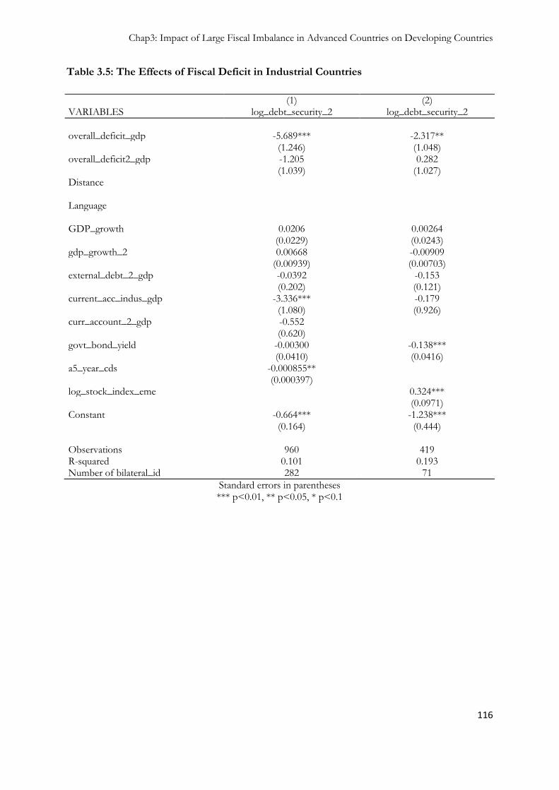
Chap3: Impact of Large Fiscal Imbalance in Advanced Countries on Developing Countries
116
Table 3.5: The Effects of Fiscal Deficit in Industrial Countries
(1) (2) VARIABLES log_debt_security_2 log_debt_security_2
overall_deficit_gdp -5.689*** -2.317** (1.246) (1.048) overall_deficit2_gdp -1.205 0.282 (1.039) (1.027) Distance Language GDP_growth 0.0206 0.00264 (0.0229) (0.0243) gdp_growth_2 0.00668 -0.00909 (0.00939) (0.00703) external_debt_2_gdp -0.0392 -0.153 (0.202) (0.121) current_acc_indus_gdp -3.336*** -0.179 (1.080) (0.926) curr_account_2_gdp -0.552 (0.620) govt_bond_yield -0.00300 -0.138*** (0.0410) (0.0416) a5_year_cds -0.000855** (0.000397) log_stock_index_eme 0.324*** (0.0971) Constant -0.664*** -1.238*** (0.164) (0.444) Observations 960 419 R-squared 0.101 0.193 Number of bilateral_id 282 71
Standard errors in parentheses *** p<0.01, ** p<0.05, * p<0.1

Chap3: Impact of Large Fiscal Imbalance in Advanced Countries on Developing Countries
117
Indeed during good times in Western countries, investors are more confident and
developing countries receive more capital flows.
When I consider now the level of external debt (Table 3.4, column-1), the results are
consistent with those of Baldacci & al. 2008. The higher the external debt (in percent of
GDP), the less attractive the bonds of developing economies, since the risk of default or
debt rescheduling increases.
The current account deficit in source countries comes with a negative sign as expected.
Since capital outflow in industrial countries improve the current account balance.
The results also confirm the high importance of “push factors” for capital inflows to
EMEs. A high level of stock market index in EMEs (Table 3.4 column-3) encourages
capital inflow motivated by return from investments. But when the rate of return is higher
in industrial countries (government bond yield on Table 3.4 column-3) investments in
developing countries diminish, as investors prefer source country bonds.
The interesting thing is that when some control variables are introduced in the
estimations, the fiscal deficit and the output growth in EMEs are no longer significant.
Actually this highlights the fact that the decision to purchase bonds issued by EMEs is
made (almost) solely based on the relative profitability of this investment. When the stock
market index and government bond yields are considered, EMEs variables become less
important in explaining capital flows (Table 3.4 Column-3). The level of risk on EMEs
bonds (approximated by the 5-year Credit Default Swap (CDS), as expected, has a
negative impact on portfolio investment in developing economies (Table 3.5 Column-1).
Moreover when the 5-year CDS is introduced, the negative impact of fiscal deficit in
industrial countries is greater and all other control variables (such as GDP growth in both
sets of countries) become statistically insignificant. Thus, this confirms the assumption
that large deficits in advanced countries always cause financial risks to increase in
developing countries.
Summing up all the previous findings, one can reasonably say that the effect of fiscal
deficit in industrial countries on capital flows to EMEs is strongly negative. Table A.3.8

Chap3: Impact of Large Fiscal Imbalance in Advanced Countries on Developing Countries
118
presents in greater detail, this impact on each developing country if you choose a marginal
impact of 4 and 952.
In the following section, the investigation will answer the question of whether the stock
of debt in advanced economies has the same impact as their fiscal deficit on portfolio
investment.
3.5.2 The effects of Public Debt
Following the previous analysis, we estimate here the effect of industrial countries‟
government debt on bond purchases. This will allow us to see whether investors are also
sensitive to the stock of public deficit. Indeed, if capital owners adjust their investment
according to the level of debt, this would mean that they assess the sustainability of the
source country‟s current fiscal policy. Once this policy is considered unsustainable53
(meaning that if the government keeps pursuing the current policy they will not be able to
repay the debt and a restrictive fiscal policy will be unavoidable), portfolio investments are
reduced or capital is withdrawn from developing countries since a worsening of the
situation is expected (countercyclicality argument). This is simply due to the argument
developed earlier that when governments of western countries have higher capital needs
this creates a crowding-out effect in developing economies.
52 Indicative marginal effects.
53 Several methods allow assessing the sustainability of the fiscal policy among which one can cite the
Solvency Condition. The solvency condition states that the public sector is solvent if the present
discounted value of government current and future spending is at least equal or lower than the present
discounted value of government current and future path income net of any initial indebtness. Another
method would be to look at the gap between real interest rate and real growth rate, if the latter is greater
public debt therefore needs to be stabilized.
Chap3: Impact of Large Fiscal Imbalance in Advanced Countries on Developing Countries
119
3.5.2.1 The Results
Table 3.6 presents the results from both the invariable characteristics and bilateral
fixed effects of industrial countries. The first fact that comes out of these sets of
estimation is that advanced countries‟ government debt is statistically significant only
when Bilateral fixed effects are used. Therefore, even if both results are presented, the
focus will be on outcomes from estimations using bilateral fixed effects.
Table-3.6 Column-1 shows roughly the main results when only industrial countries‟ fixed
effects are considered. Compared to Column-2, the results are similar except for the
variable of interest (government debt). First the gravity variables, distance and language
dummy, behave quite well with distance between countries impacting negatively on capital
flows (same as in previous results). Higher government net debt, therefore higher
borrowing needs, crowds out portfolio investment in developing countries. Developing
countries‟ external debt, as previously indicated and consistent with Baldacci & al. 2008,
still discourage capital inflows.
Since the stock of debt is considered as an indicator of the sustainability of the fiscal
policies of industrial countries, it becomes reasonable for “push factors” to be more
visible. Indeed when there is any risk in investing in EMEs (due to fiscal turmoil in
advanced economies), all other EME variables might not be relevant for investors while
making their decision. For instance, in all estimations, GDP growth in developing
economies is not statistically significant (Table-3.6 Column-2).
The remaining tables show a normal sign for current account deficit in industrial
countries. Table-3.8 Column-2 underlines an important result consistent with previous
findings. Indeed as soon as the level of risk is included, captured by the CDS, one
observes a direct outflow of capital without any consideration to the rates of return. This
result suggests that even if returns on bonds in industrial countries are low and/or stock
market index in EMEs is high, as soon as the level of risk increases capital will flee toward
safer shelters in developed economies.
Based on this set of estimations using developed economies‟ net public debt as a variable
of interest, it appears that the effects on capital flows are similar to the effects of fiscal

Chap3: Impact of Large Fiscal Imbalance in Advanced Countries on Developing Countries
120
deficit. This similarity is not surprising since both variables (fiscal deficit and public debt)
indicate the wellbeing of the real economy in industrial countries.
The next section will be the place to undertake some robustness check and further
investigation.
Table 3.6: Effects of Industrial Countries’ government net debt
(1) (2) VARIABLES Indus FE Bilateral FE
log_gov_debt -0.208 -0.262** (0.189) (0.105) overall_deficit2_gdp -3.272*** -2.697*** (0.564) (0.567) Distance -0.553*** (0.0788) Language 0.0333 (0.0773) external_debt_2_gdp -0.538*** -0.289*** (0.0928) (0.110) GDP_growth 0.163*** 0.143*** (0.0277) (0.0162) gdp_growth_2 -0.0314*** 0.00195 (0.00617) (0.00385) Constant 1.756*** -0.411 (0.633) (0.313) Observations 1732 1732 R-squared 0.093 0.145 Number of indus_id 15 Number of bilateral_id 295
Standard errors in parentheses *** p<0.01, ** p<0.05, * p<0.1

Chap3: Impact of Large Fiscal Imbalance in Advanced Countries on Developing Countries
121
Table3.7: Effects of industrial countries’ government net debt
(1) (2) VARIABLES Indus FE Bilateral FE
log_gov_debt -0.226 -0.210** (0.191) (0.105) overall_deficit2_gdp -2.492*** -2.538*** (0.550) (0.538) Distance -0.436*** (0.0767) Language 0.0175 (0.0785) external_debt_2_gdp -0.569*** -0.224** (0.0939) (0.112) GDP_growth 0.128*** 0.160*** (0.0274) (0.0161) current_acc_indus_gdp -2.105 -3.407*** (1.287) (0.717) curr_account_2_gdp -0.871** -0.137 (0.418) (0.450) Constant 1.340** -0.594* (0.635) (0.313) Observations 1732 1732 R-squared 0.083 0.158 Number of indus_id 15 Number of bilateral_id 295
Standard errors in parentheses *** p<0.01, ** p<0.05, * p<0.1

Chap3: Impact of Large Fiscal Imbalance in Advanced Countries on Developing Countries
122
Table 3.8: Effects of industrial countries’ government net debt
(1) (2) VARIABLES Indus FE Bilateral FE
log_gov_debt -0.159 -0.332* (0.191) (0.183) overall_deficit2_gdp -2.128*** 0.679 (0.559) (1.881) external_debt_2_gdp -0.557*** -0.400** (0.0936) (0.172) GDP_growth 0.108*** 0.0604** (0.0279) (0.0257) gdp_growth_2 -0.0438 (0.0351) current_acc_indus_gdp -2.006 0.978 (1.283) (1.313) curr_account_2_gdp -0.842** 2.752 (0.416) (3.521) govt_bond_yield -0.165*** -0.0833 (0.0486) (0.0555) stock_index_eme -5.65e-06 (3.56e-06) 5_year_cds -0.000413** (0.000181) distance -0.430*** (0.0765) language 7.64e-05 (0.0784) Constant 1.829*** 0.926 (0.649) (0.561) Observations 1732 195 R-squared 0.089 0.127 Number of indus_id 15 Number of bilateral_id 52
Standard errors in parentheses *** p<0.01, ** p<0.05, * p<0.1

Chap3: Impact of Large Fiscal Imbalance in Advanced Countries on Developing Countries
123
3.6 Further Analysis and some Robustness check
First a robustness check is implemented on the baseline estimation using the
Heckman selectivity correction. The results (Table A.3.5) show the countries selected are
those with the highest output growth (advanced and emerging economies as well), and
EMEs in the sample seem to have better current account positions. Despite these
possible biases the results remain strongly similar to the baseline estimation outputs.
3.6.1 Countries with previous default
The last century and the early years of the 21st have seen the debt burden of some
countries reaching unsustainable and unaffordable levels. Markets anticipated a default
and in most situations this prediction came true due to speculative attacks and higher
premiums requested. One can make the hypothesis that not all EMEs face the same level
of risk and for some, particularly developing countries in periods of global economic
crisis, the effect of fiscal deficit in developed countries is not the same for them. The
countries that have defaulted in the past (or recently) might be perceived as more risky
than other developing countries. If this argument is relevant, the industrial countries‟
fiscal deficit combined with the default dummy variable should have an important
influence on bonds trade. Therefore to capture this fact, I construct a dummy variable
equal to 1 for countries that have defaulted54 at least once in the past and 0 otherwise,
then this variable is introduced multiplicatively with fiscal deficit in advanced countries to
see if there is a special treatment for these countries. When introduced (TableA.3.2), this
variable becomes non-significant and leaves previous results perfectly stable. It appears
that the effect of a fiscal stance in advanced countries is not discriminative with regard to
54 According to Moody‟s data base, sovereign default was recorded 12 times in the recent period,
from 1983 to 2007. Exactly 11 countries were concerned with Ukraine defaulting during two different
periods. These countries are: Venezuela (07/1998), Russia (08/1998), Ukraine (09/1998), Pakistan
(07/1999), Ecuador (08/1999), Ukraine (01/2000), Peru (09/2000), Argentina (11/2001), Moldova
(06/2002), Uruguay (05/2003), Dominican Republic (04/2005), Belize (12/2006).

Chap3: Impact of Large Fiscal Imbalance in Advanced Countries on Developing Countries
124
a previous sovereign default on external debt; investors award the same level of risk to all
countries in our sample.
3.6.2 Episodes of large fiscal deficit in advanced economies
One should distinguish between a normal situation and an episode of “severe” fiscal
imbalances. Indeed the results available until now could be qualified as being in line with a
general rule but one can ask what should be the case during periods of unusually high
deficit? To do so, episodes of large fiscal deficit were defined as periods during which the
overall deficit for a country is above the mean plus one standard deviation. We construct
a dummy variable to capture this fact (equal to 1 if the deficit is higher than the mean plus
one standard deviation). Then, the latter variable is interacted with the fiscal deficit in
advanced countries. However the interactive term (fiscal deficit*dummy) is not
statistically significant. The reason for this curious result could be that very few
observations correspond to this definition of high deficit. Indeed the period 2001-2007
was mainly characterized by fiscal soundness in industrial countries (no major fiscal shock
was noticed in the data). But the overall deficit in advanced countries coefficient, still
statistically very significant, goes up. Even if the interactive term is not significant, the
high coefficient of fiscal deficit shows us that it has a particular impact during episodes of
large deficit. This coefficient might suggest that when there is a change in the fiscal policy
path, namely a period of severe crisis, (for instance an expansive fiscal policy) the quantity
of investments drying out increases.
3.6.3 Testing for non-linear effects and further analysis
Here I will be testing for changes in the effect of industrial countries‟ fiscal deficit
(and debt) on bonds sale. Namely, can “extreme” level of deficit lead to a race toward
developing countries‟ financial assets? A positive answer to this question could be the sign
of the birth of a new period.
Chap3: Impact of Large Fiscal Imbalance in Advanced Countries on Developing Countries
125
When I introduce the square of the advanced countries fiscal deficit, this coefficient
comes positive and statistically significant. This means that above a certain limit, fiscal
deficit in industrial countries reaches a level believed by investors as unsustainable.
Therefore for bond holders a sovereign default by developed western government is no
longer an unthinkable scenario (TableA.3.4). This would mean that at a certain point, the
old rules of fixed income world are being outdated. Indeed, until recently developing
countries‟ debt was viewed as too risky compared for instance to western European
assets. A key question one could ask is whether this theoretical result is consistent with
the actual situation in the world economy? Indeed the recent fiscal turmoil in the
developed world confirms this result in a quite eloquent manner.
After the onset of the financial crisis, in late 2008, one saw a sudden drop in investments
in developing countries and capital outflow. According to analysts, (e.g. Kapur & Rakesh
2010) this capital outflow has different determinants from the previous ones. In the past
crisis, capital was fleeing from EMEs due to poor sovereign (as well as corporate)
solvency. More recently, late 2008, capital outflow was mainly motivated by deleveraging55
motives (Kapur & Rakesh 2010). One year later the portfolio investment on bonds
resumed while fiscal deficits and public debt were at their highest level in advanced
countries. Two arguments could explain these facts.
First the quantitative easing policy in major economies (USA, UK)56 flooded the economy
with cheap money. For investors it therefore became possible to arbitrate between cheap
money at home (with lower return at home as well) and higher yields abroad especially in
EMEs. This is the so called “Carry Trade”57. As narrowly defined, the carry trade is the
55 Deleveraging consists simply of reducing the debt to total assets ratio and thus cleaning one‟s
balance sheet.
56 The ECB, from late 2008, maintained its interest rates at a low level of 1% in order to ease access
to liquidity for banks.
57 In the early 2000s, the Yen served as fuel for carry traders and recently history repeated itself with
the US dollars. For instance the recent world financial crisis, which induced a weaker US dollar and
lower interest rate, some investors might find profitable to borrow in dollar and invest in some
Chap3: Impact of Large Fiscal Imbalance in Advanced Countries on Developing Countries
126
practice of borrowing currency from a country where interest rates are low and then
lending the proceeds in the currency of a country where interest rates are higher. The goal
is to profit from the interest rate differential (Grenville Stephen, 2010). And this was
among the determinants in the re-surge of bond investments in developing countries in
late 2009. FigA.3.1 shows clearly that after 2008 outflow, capital movement toward
developing economies resumed progressively.
The second argument also linked to the previous one is the unprecedented level of public
sector deficits and debt in the developed world. In the USA, the debt burden is expected
to rise to more than 90% of GDP by 2011, in UK the public debt in 2010 represents
79.1% of GDP (a fiscal deficit more than 12% of GDP)58, in Spain, Greece and France
the public debt is also above 70% of GDP (and fiscal deficit nearly reaching 11% of
GDP). On the other hand, for investors Brazilian, Mexican, Chinese, even Russian (that
defaulted in 1998) bonds are less risky than Euro Zone ones. The reason for this reversal
is that most of middle income economies have strong economies, low budget deficits and
current account surpluses59. So the fundamentals look much better than in major
developed economies such as USA, Japan, UK and in most Euro area countries.
Additional to the fiscal turmoil in major developed countries, the growth prospects are
also relatively weak (FigA.3.3). Consequently investors believe that nothing in the medium
term can be in favour of an improvement of the fiscal stance. The purchases of
developing countries‟ bonds in 2010 (from January to early May) have reached 15.3 billion
US dollars and, this inflow has never been seen before. Moreover the EMEs sovereign
bond index spreads (compared to US bond yields) have been tightening since October
2008 (based on JPMorgan data, this gap is around 1.48% in 2010 compared to 2.58% in
2005).
developing economies where one might have double returns. Indeed one gets profit from the
exchange rate arbitrage and from the yields difference.
58 The Institute for Fiscal Studies database, “Debt and Borrowing” data.
59 This was a great achievement for EMEs since they learnt from previous crises. Therefore more
prudential fiscal and monetary policies were implemented during the boom period. After 2007, in the
middle of the crisis these countries had enough possibilities to support their economies with fiscal
and monetary stimulus packages.

Chap3: Impact of Large Fiscal Imbalance in Advanced Countries on Developing Countries
127
At the same time countries, despite the “safe” Euro shelter, are struggling to have access
to private capital in the bond market. Indeed for Greece, Spain, Portugal, perhaps later
Ireland and Italy debt restructuring (or default) is not excluded60.
This situation could mark the start of a new paradigm or at least the end of the one that
sees developing countries as fiscally irresponsible, with huge deficits and procyclical fiscal
policies. And developed countries being characterized by sound and consistent fiscal
policies. Even if it becomes evident that this paradigm has ended or is living its last
moments, as soon as data becomes available, further investigation should be done on this
issue. Right now, one can only say that the developed world bonds are not the only ones
holding the label “safety guaranteed” FigA.3.2.
60The first results on the non linear effects were anterior to the crisis in the Euro area. Then the
Greek (and Spain?) crisis helped to interpret such results which were incomprehensible before.

Chap3: Impact of Large Fiscal Imbalance in Advanced Countries on Developing Countries
128
3.7 Conclusion
It comes out of this paper that higher fiscal deficit in industrial countries crowds out
capital flows to emerging market economies. We showed that if one considers the specific
variables for EME and industrial countries and the shared variables as well, the overall
deficit in rich countries lowers significantly capital flows to developing countries. While
the deficit of developing countries lowers also, but with less intensity, the variable of
interest. Indeed in recession periods, governments in advanced economies, by
implementing countercyclical policies increase their deficit in order to stabilize the real
economy. But in doing so, they compete with developing countries for access to capital.
Moreover, investors‟ confidence falls (due to lower exportation by EMEs), and all of
these effects contribute to reducing capital flows.
It was found also that all developing countries share the same level of risk since the fact
that the country has defaulted or not is not relevant to investors. Therefore when the
CDS level increases it affects almost all countries in the same way.
However these results need to be a bit nuanced, because the (old) paradigm arguing that
developing countries‟ cycles are indefinitely synchronized to those of advanced countries
doesn‟t seem to hold. The recovery path from the 2007 global crisis has shown recently
that developing countries are leading the global economic recovery while major countries
like USA, UK and Euro zone faced low GDP growth prospects. Also, a non-linear
investigation outcome shed light on this issue. Above a certain level of fiscal deficit,
considered as unsustainable by investors, the risk of default by a Western country
becomes non-negligible; they withdraw their capital from former “safe countries” in
favour of emerging economies. The first quarter of 2010 has clearly shown that financial
markets were worried about the fiscal stance in advanced countries. And the markets have
forced, with higher premiums on sovereign borrowings, governments to tighten their
fiscal policy (earlier than predicted) and reduce debt to more reasonable levels.
Nevertheless after full recovery, it would be interesting to check whether this result was
cyclical or a deeper change.

Chap3: Impact of Large Fiscal Imbalance in Advanced Countries on Developing Countries
129
Before any policy recommendation, one has to notice that EMEs have learnt from their
previous experiences during past crises. At the onset of this crisis developing countries
were in a good position with current account surpluses, low (or surplus sometimes) fiscal
deficit, negligible external debt, and huge foreign reserves; owing to prudent policies. In
order to stay as much as possible safe from fiscal (and financial) turmoil in developed
countries, financial integration between EMEs should deepen. Trade in goods between
developing economies should also increasingly concern finished product so they can stay
safe from any crunch in Western economies.
All along this article emerging market and developing countries were employed as
synonyms. Obviously any low income country was among the sample used here and, two
reasons explain this. First low income countries essentially borrow capital from bilateral
or institutional partners, and international bond negotiations are extremely scarce. Second,
low income countries due to high levels of debt and poor governance do not have access
to capital from the financial market (at least for the bond market), except of course FDI
flows.
Despite these relevant results, the database only concerns bonds exchanged in the primary
market. In other worlds, after purchasing a developing country‟s bond, an investor can re-
sell it in the secondary market. In this situation, the coefficient estimated could be higher
than the actual impact of advanced countries deficit on bond purchases. For instance
despite a situation of crisis, a speculator can buy a EMEs bond in the secondary market at
a lower price and bets on an increase of its value in the future. On a large scale, trading in
the secondary market will be a non-negligible source of funding for developing countries.
Even though such data are not available (or not easily accessible), this does not affect our
results which focuses mainly on the primary bonds markets.

Chap3: Impact of Large Fiscal Imbalance in Advanced Countries on Developing Countries
130
ANNEXES CHAPTER 3

Chap3: Impact of Large Fiscal Imbalance in Advanced Countries on Developing Countries
131
Table A.3.1: Data used gravity estimations: from 2001 to 2007.
Notation Definition Source
Dependent variable:
log_debt_securities2
Total debt securities hold by
non-resident. (annual frequency)
CPIS database available online at: http://www.imf.org/external/np/sta/pi/datarsl.htm
Overall_deficit_gdp Overall fiscal deficit for
industrial countries over GDP
(annual frequency)
World Economic Outlook, 2009.
Overall_deficit2_gdp Overall fiscal deficit for emerging
countries over GDP (annual
frequency)
World Economic Outlook, 2009.
Gdp_growth Real GDP growth for industrial
countries. (annual frequency)
World Economic Outlook, 2009.
Gdp_growth_2 Real GDP growth for emerging
countries. (annual frequency)
World Economic Outlook, 2009.
Ln_distance Natural log of distance between
capital cities of EMEs and their
industrial country partners, (in
kilometres).
CPII (French research center in
international economics). Data
available online at: http://www.cepii.fr/francgraph/bdd/distances.htm
lang Dummy of common language. CPII (French research center in
international economics). Data
available online at: http://www.cepii.fr/francgraph/bdd/distances.htm
external_debt_2_gdp Total external debt stock over
GDP, for emerging countries.
(annual frequency)
World Economic Outlook, 2009.
current_acc_indus_gdp
Industrial economies Current
account balance (annual
frequency) in percent of GDP.
Annual data.
International Financial Statistics.
curr_account_eme_gdp Emerging economies Current
account balance (annual
frequency) in percent of GDP.
Annual data.
International Financial Statistics.
stock_index_eme Stock market index of emerging
countries. (annual frequency)
Global Data Source
govt_bond_yield 5-year emerging government Datastream. (Credit Market Analysis

Chap3: Impact of Large Fiscal Imbalance in Advanced Countries on Developing Countries
132
bond yield database, CMA)
5_year_cds Sovereign 5-year Credit default
swap on emerging market bonds.
Datastream. (Credit Market Analysis
database, CMA)
default Dummy variable= 1 if the
country has defaulted in the past,
and 0 otherwise.
Moody‟s Global Credit Research,
March 2008.
default_risk The interaction between the
dummy default and the overall
deficit in industrial countries
Large_deficit_dummy Interactive variable between
dummy of large fiscal (mean +1
SD) and the overall deficit in
industrial countries in percent of
GDP.

Chap3: Impact of Large Fiscal Imbalance in Advanced Countries on Developing Countries
133
FigA.3.1: Portfolio, Equity Investment evolution: Prospects after the financial Crisis.
FigA.3.2: Government Bond Yields comparison across countries

Chap3: Impact of Large Fiscal Imbalance in Advanced Countries on Developing Countries
134
FigA.3.3: GDP Evolution across countries in recent period.
FigA.3.4: Evolution of public and private saving in the USA compared to fiscal deficit.
In billions USD

Chap3: Impact of Large Fiscal Imbalance in Advanced Countries on Developing Countries
135
Fig A.3.5: LIBOR as Global Interest Rates
Fig A.3.6: Budget Deficit in Industrial Countries

Chap3: Impact of Large Fiscal Imbalance in Advanced Countries on Developing Countries
136
Fig A.3.7: Government Debt Budget Deficit in Industrial Countries
FigA.3.8: Portfolio Investment per income level
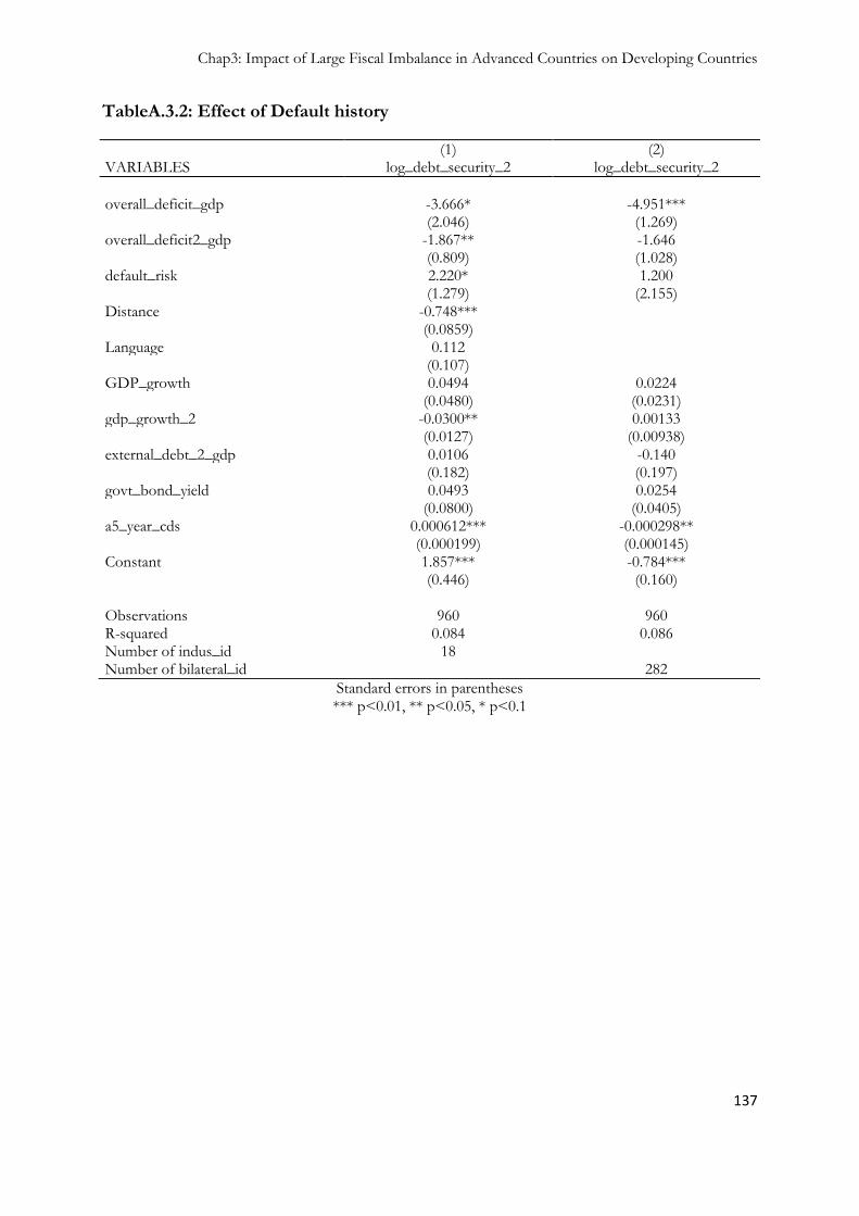
Chap3: Impact of Large Fiscal Imbalance in Advanced Countries on Developing Countries
137
TableA.3.2: Effect of Default history
(1) (2) VARIABLES log_debt_security_2 log_debt_security_2
overall_deficit_gdp -3.666* -4.951*** (2.046) (1.269) overall_deficit2_gdp -1.867** -1.646 (0.809) (1.028) default_risk 2.220* 1.200 (1.279) (2.155) Distance -0.748*** (0.0859) Language 0.112 (0.107) GDP_growth 0.0494 0.0224 (0.0480) (0.0231) gdp_growth_2 -0.0300** 0.00133 (0.0127) (0.00938) external_debt_2_gdp 0.0106 -0.140 (0.182) (0.197) govt_bond_yield 0.0493 0.0254 (0.0800) (0.0405) a5_year_cds 0.000612*** -0.000298** (0.000199) (0.000145) Constant 1.857*** -0.784*** (0.446) (0.160) Observations 960 960 R-squared 0.084 0.086 Number of indus_id 18 Number of bilateral_id 282
Standard errors in parentheses *** p<0.01, ** p<0.05, * p<0.1
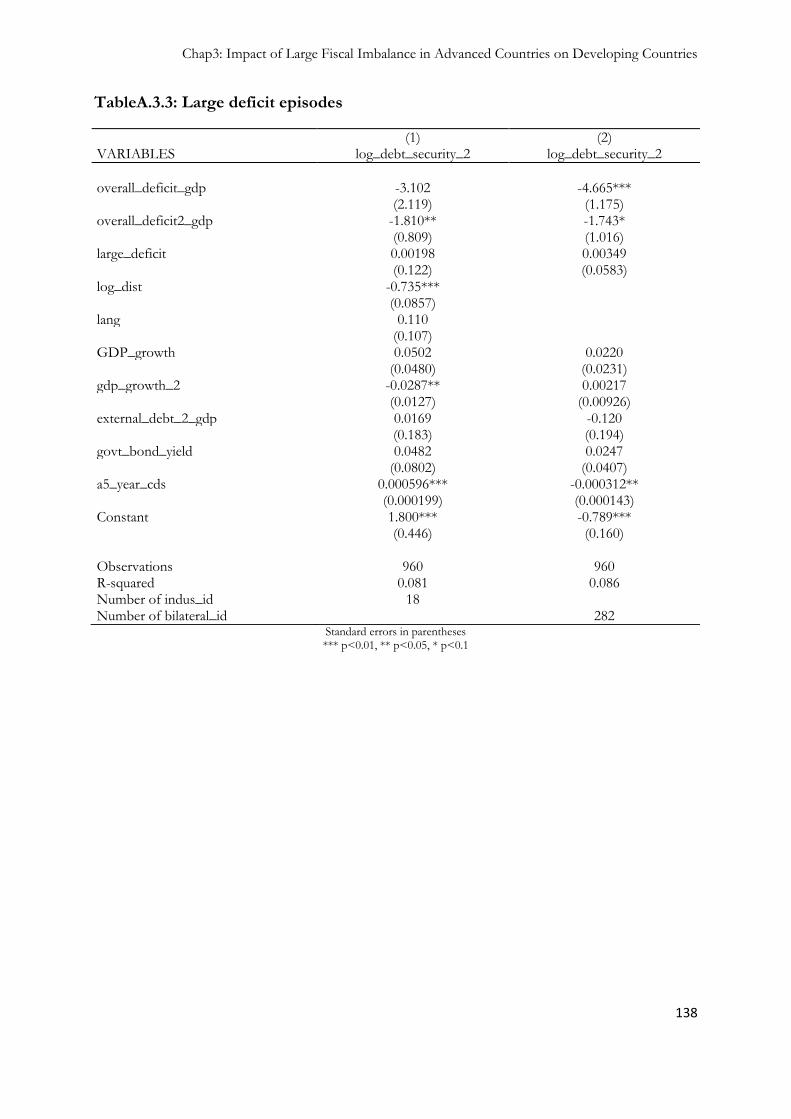
Chap3: Impact of Large Fiscal Imbalance in Advanced Countries on Developing Countries
138
TableA.3.3: Large deficit episodes
(1) (2) VARIABLES log_debt_security_2 log_debt_security_2
overall_deficit_gdp -3.102 -4.665*** (2.119) (1.175) overall_deficit2_gdp -1.810** -1.743* (0.809) (1.016) large_deficit 0.00198 0.00349 (0.122) (0.0583) log_dist -0.735*** (0.0857) lang 0.110 (0.107) GDP_growth 0.0502 0.0220 (0.0480) (0.0231) gdp_growth_2 -0.0287** 0.00217 (0.0127) (0.00926) external_debt_2_gdp 0.0169 -0.120 (0.183) (0.194) govt_bond_yield 0.0482 0.0247 (0.0802) (0.0407) a5_year_cds 0.000596*** -0.000312** (0.000199) (0.000143) Constant 1.800*** -0.789*** (0.446) (0.160) Observations 960 960 R-squared 0.081 0.086 Number of indus_id 18 Number of bilateral_id 282
Standard errors in parentheses *** p<0.01, ** p<0.05, * p<0.1

Chap3: Impact of Large Fiscal Imbalance in Advanced Countries on Developing Countries
139
Table A.3.4: Test for non-linear effect of Fiscal deficit in advanced economies
(1) VARIABLES log_debt_security_2
overall_deficit_gdp -9.781*** (1.764) overall_deficit_gdp^2 3.199* (1.787) curr_account_2_gdp 0.696 (0.908) overall_deficit2_gdp -13.25*** (1.036) Constant -1.933*** (0.0418) Observations 2482 Number of bilateral_id 419 R-squared 0.104
Standard errors in parentheses *** p<0.01, ** p<0.05, * p<0.1

Chap3: Impact of Large Fiscal Imbalance in Advanced Countries on Developing Countries
140
TableA.3.5: Heckman Selectivity Bias Correction
(1) (2) (3) VARIABLES log_debt_security_2 select mills
overall_deficit_gdp -7.957***
(0.821)
overall_deficit2_gdp -3.908***
(0.730)
log_dist -0.455***
(0.0916)
lang 0.305***
(0.0902)
GDP_growth 0.247*** 0.130***
(0.0516) (0.0120)
gdp_growth_2 0.0130 0.0390***
(0.0170) (0.00604)
external_debt_2_gdp -0.676***
(0.115)
govt_bond_yield -0.0823***
(0.0292)
current_acc_indus_gdp -0.136
(0.408)
curr_account_2_gdp 1.844***
(0.425)
lambda 1.764**
(0.685)
Constant -0.219
(0.675)
Observations 2712 2712 2712 Standard errors in parentheses
*** p<0.01, ** p<0.05, * p<0.1
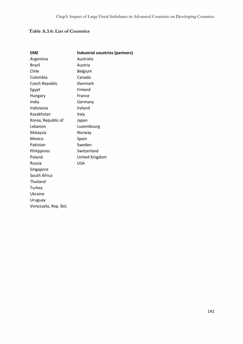
Chap3: Impact of Large Fiscal Imbalance in Advanced Countries on Developing Countries
141
Table A.3.6: List of Countries
EME Industrial countries (partners)
Argentina Australia
Brazil Austria
Chile Belgium
Colombia Canada
Czech Republic Danmark
Egypt Finland
Hungary France
India Germany
Indonesia Ireland
Kazakhstan Italy
Korea, Republic of Japan
Lebanon Luxembourg
Malaysia Norway
Mexico Spain
Pakistan Sweden
Philippines Switzerland
Poland United Kingdom
Russia USA
Singapore South Africa Thailand Turkey Ukraine Uruguay Venezuela, Rep. Bol.

Chap3: Impact of Large Fiscal Imbalance in Advanced Countries on Developing Countries
142
Emerging Market Economies 2001 2002 2003 2004 2005 2006 2007
Argentina 20,2135988 12,0512427 14,84813265 22,6440529 21,2626126 28,8482692 23,9535992
Brazil 32,7932791 29,8009002 42,71421017 45,7438385 45,5502463 47,7849384 47,9262259
Chile 4,67804861 5,91763623 8,690728487 10,486016 10,3301313 10,0184015 9,0398209
Colombia 5,18280576 4,11041208 5,390877776 7,06159237 6,82273528 9,74549021 10,5626153
Czech Republic 0,92430026 1,25391389 2,032604968 6,57370386 8,07199177 9,66907489 11,8639581
Egypt 0,46679471 0,23032024 0,13341374 0,18623668 2,99768638 10,4448504 5,31190793
Hungary 11,283218 15,1779654 18,40544181 29,7169284 27,5098044 38,299947 45,2127409
India 1,3319923 0,63425535 0,668670887 3,02790024 6,34323942 10,7855952 7,81571885
Indonesia 0,82617379 0,93595812 1,542644613 1,89686839 4,77054361 7,01849582 7,65399782
Kazakhstan 0,2667178 0,1633899 0,207881489 1,09926246 1,9386824 5,46151842 1,60718684
Korea, Republic of 17,7355249 18,8592426 13,28675823 24,5129483 29,9682833 35,763395 54,1942114
Lebanon 0,33659113 0,12253173 0,159760991 0,92050429 0,66960265 1,35266114 0,88868932
Malaysia 5,54978873 6,37355149 8,899041378 11,9517866 13,3146288 14,9779449 18,1560648
Mexico 38,944225 39,7929232 43,61005904 47,3749417 53,7457806 50,3328553 46,5778904
Pakistan 0,17448557 0,09805692 0,060597489 0,15917301 0,09497859 0,73021496 0,87684137
Philippines 6,45401654 6,57093926 9,942804167 10,4036327 14,242407 17,2146028 17,0417561
Poland 5,89158171 10,1697224 16,69905114 32,069651 44,0658511 49,418353 54,6720256
Russia 13,6208786 16,1344907 18,79732069 23,7795795 19,0493735 34,5359609 31,5836017
Singapore 11,203308 6,52799134 7,96613773 12,4757594 18,9958937 22,7165174 26,7246961
South Africa 6,14303513 6,62794806 11,21277915 13,9824335 15,9617414 15,7689611 17,6594652
Thailand 2,27413414 1,76825638 2,213316781 2,60040958 3,05269723 4,09866741 2,12823758
Turkey 11,1418409 10,0973892 10,73380633 14,3559091 20,1839554 33,4275956 32,0236165
Ukraine 0,8547097 1,29769033 1,902753075 3,51472488 3,02053825 7,74125878 7,63898009
Uruguay 1,24649995 0,96204917 1,30307472 2,27884269 2,73898858 4,12152239 4,93149874
Venezuela, Rep. Bol. 7,91576386 8,48390624 8,650560528 13,0087742 17,3090399 13,9073518 12,7286546
Annual Total Debt Securities
in billions of $US
Table A.3.7

Chap3: Impact of Large Fiscal Imbalance in Advanced Countries on Developing Countries
143
Table A.3.8: Indicative values of Marginal effects of Fiscal deficit in industrial countries on portfolio investment
Emerging Market Economies Mean 4% 9%
20,5459297 0,82183719 1,84913367
Argentina 41,7590912 1,67036365 3,75831821
Brazil 8,45154043 0,33806162 0,76063864
Chile 6,98236125 0,27929445 0,62841251
Colombia 5,76993539 0,23079742 0,51929419
Czech Republic 2,82445858 0,11297834 0,25420127
Egypt 26,5151494 1,06060598 2,38636345
Hungary 4,37248175 0,17489927 0,39352336
India 3,52066888 0,14082676 0,3168602
Indonesia 1,53494847 0,06139794 0,13814536
Kazakhstan 27,760052 1,11040208 2,49840468
Korea, Republic of 0,63576304 0,02543052 0,05721867
Lebanon 11,3175438 0,45270175 1,01857894
Malaysia 45,7683822 1,83073529 4,1191544
Mexico 0,31347827 0,01253913 0,02821304
Pakistan 11,6957369 0,46782948 1,05261632
Philippines 30,4266051 1,21706421 2,73839446
Poland 22,5001722 0,90000689 2,0250155
Russia 15,2300434 0,60920174 1,37070391
Singapore 12,4794805 0,49917922 1,12315325
South Africa 2,59081701 0,10363268 0,23317353
Thailand 18,8520162 0,75408065 1,69668146
Turkey 3,71009359 0,14840374 0,33390842
Ukraine 2,51178232 0,10047129 0,22606041
Uruguay 11,7148644 0,46859458 1,0543378
Venezuela, Rep. Bol.
Note: This table presents the mean of yearly value of total debt securities from 2001 to 2007.
The 4% (9%) column represents the effect of a 4% (9%) increase in overall fiscal deficit in
industrial countries.
Values are in Billions of US dollars.

Chap3: Impact of Large Fiscal Imbalance in Advanced Countries on Developing Countries
144

Chap4: Fiscal Policy for Stabilization in Developing Countries: A Comparative Approach
145
Chapter 4: Fiscal Policy for
Stabilization in Developing
Countries: A Comparative
Approach

Chap4: Fiscal Policy for Stabilization in Developing Countries: A Comparative Approach
146
4.1 Introduction
The issue of efficiency of macroeconomic policies on short term economic activity
has remained an unsolved question where several theories give different predications. A
first set of studies has tried to define the nature of and how policy makers were using
macroeconomic policies to influence the real economy. These studies reveal that OECD
countries (advanced economies in general) run countercyclical fiscal policies and
developing countries implement procyclical policies (details on this literature are given
later). Countercyclical fiscal policies consist in increasing budget deficit (or increasing
spending and/or reducing tax rates) when the difference between the potential output
and the current output decreases or even becomes negative. On the contrary, with
procyclical measures the government simply increases its deficit in good times (positive
output gap) and consolidates it in periods of recession. Despite these results one can
wonder if macroeconomic fluctuations are bad for economic activity and what is the
rationale behind the intervention of public authorities against these fluctuations.
The real business cycle theory argues that business cycles can be interpreted as the
economy‟s optimal response to shocks, at least in first-order approximation. While some
inefficiencies and distortions may be present in the economy, they are not viewed as
central to cyclical phenomena. Most importantly, efforts of public authorities at
stabilization may be counterproductive, and could even reduce welfare, since these
interventions might keep on track inefficient and expensive firms. Indeed recession helps
to correct organizational inefficiencies and encourage firms to reorganize, innovate or
relocate to new markets (Aghion & al. 2005). Another view similar to the neoclassical one
defends the idea that macroeconomic policy should primarily focus on price and income
stability since long-run economic growth depends only on structural characteristics such
as quality of institutions (Easterly 2005, Acemoglu & al. 2003). Therefore, and according
to these theories, even in a period of recession the government should not intervene and
stabilizing policies should remain at their lowest level possible. However for firms willing
and able to improve their efficiency, the main barrier will be access to funds in periods of
economic downturn since their profits are sliced. Therefore without an “external
intervention”, even good firms will be ejected from the market and this might delay any

Chap4: Fiscal Policy for Stabilization in Developing Countries: A Comparative Approach
147
recovery. To avoid these negative effects a government could increase public investment
or its spending and thereby foster national demand. Another possible answer from public
authorities could be to directly subsidize enterprises by supporting them in their R&D
expenses.
Moreover, according to Keynesians, recessions are considered as periods where the use
and the allocation of productive resources are inefficiently low. In a recent work, Galí &
al. 2005 identify the presence of large efficiency gaps in recession periods which are
associated with a declining aggregate efficiency. They develop a simple analytical
framework that justifies the pursuance of countercyclical fiscal policies in order to
overcome the inefficiencies associated with recessions (see infra). Finally, bailing out the
economy during bad times is sometimes almost compulsory for public authorities when
the country faces a systemic hazard. For instance, in economic crises like the recent one in
2010, without public intervention, major firms (General Motors in USA, Northern Rock
in UK etc.) could fail and leave thousands of workers unemployed and many households
losing their life-time savings. By bailing out such “too big to fail” firms, public authorities
preserve their economy from a general collapse with unpredictable social consequences.
This sheds some light on why fiscal policies should be a stabilizing tool and used by both
advanced and developing countries.
Also recent studies have shown that countercyclical public debt policy is highly growth-
enhancing (e.g. Aghion & Marinescu 2005). Therefore, even though the level of
institutional development matters, this does not exclude that cyclicality of fiscal policy
plays an important role for GDP growth.
In this chapter the contribution is twofold. Until recently, studies on the cyclicality of
fiscal policies in developing countries did consider that policies were not changing that
much, in other words a government running procyclical policies was “obliged” to
maintain such policy. What is shown here is that many developing countries were steadily
adopting better fiscal policies and therefore voracity effects were progressively
disappearing. The second aspect of this chapter is that it answers the question whether
procyclical fiscal policies are harmful always and everywhere. Indeed, one can imagine
good procyclical policies that would consist in running higher deficit in good economic

Chap4: Fiscal Policy for Stabilization in Developing Countries: A Comparative Approach
148
times to foster and strengthen economic activity. However the results in this chapter
show that countercyclical fiscal policies reduce GDP volatility and therefore reduce
uncertainty and encourage private initiatives.
The rest of this chapter is organized as follows: The next section presents the related
literature and some stylized facts of fiscal policy in developing countries. Section 3 details
theories in favor of fiscal policy as an efficient stabilizing tool. Empirical methodology
and results are presented in section 4. The last part concludes.

Chap4: Fiscal Policy for Stabilization in Developing Countries: A Comparative Approach
149
4.2 Related Literature
The investigation of what has been done by researchers in the field can be divided
into two components. The first is a positive analysis and the second a normative analysis.
In the positive analysis area, people are interested in the real nature or the effective
behaviour (whether a government pursues a pro or a countercyclical policy) of fiscal
authorities (e.g. Rand & Tarp, 2002). The normative analysis gives details and evidences
on how the fiscal tool should be used to avoid loss of efficiency and to get less
macroeconomic fluctuations. A deeper look at what has been done allows us to say that
the two analyses are unequally treated in the literature (in terms of quantity of papers
dedicated); a clear advantage being given to the positive analysis area. In this paper
however, both analyses, normative and positive, are empirically tested showing why
countercyclical fiscal policies are preferable to procyclical ones.
4.2.1 Main characteristics of fiscal policy in developing countries
The first step will be to investigate the main characteristics of fiscal policy in
developing countries. As said above it is commonly admitted in the literature that fiscal
policy is procyclical in many non-OECD countries. In what follows, one will investigate
these facts and arguments in the literature for developing countries.
In economic theory, a common wisdom would advise that fiscal policy, namely
government spending and tax revenue, is to remain constant throughout the business
cycle. In other words, fiscal policy will follow a countercyclical rule (spending going down
and tax revenues increasing in good times and public expenditures going up and tax
revenues decreasing in recession periods) so the budget surplus, as a share of GDP,
should increase during economic booms and decrease during recession. This is the case if
policymakers follow the Keynesian prescriptions. One the other side, tax smoothing
models inspired by Barro 1979 suggest that fiscal policy should remain neutral all along
the business cycle, i.e. one should have zero correlation between government spending

Chap4: Fiscal Policy for Stabilization in Developing Countries: A Comparative Approach
150
and output (Lucas & Stokey, 1983). As said above the dominant thought is that fiscal
policy should be countercyclical.
Alesina & Tabellini 2005 try to test for this effect in developing countries61. They found
that in developing countries fiscal authority behave differently and conduct procyclical
policy. Indeed during expansions, government spending as a share of GDP increases and
goes down in bad times (the budget deficit follows the same path, increasing in good
times and decreasing in recessions). They develop a model considering that the
procyclicality arises much more from voters due to a lack of information and a political
agency problem. There are two actors in the model, the government and the private
sector consisting of a representative consumer. The private agent maximizes the value of
his expected utility from private consumption. The model is as follows:
The expected utility from consumption is as follow:0
( )ttt
E u c
. tc is the
consumption in period t, E the expectations factor, u (.) is a smooth and strictly concave
increasing factor. In this model one considers that the government uses all its tax revenue
for non productive expenditures (rents) and the private agents focus only on controlling
the government agency problem. tr is the total of non-productive spending62 in the
form of rent solely benefiting the government. These rents are financed through t
unproductive taxes paid by consumers. Still for the government, it issues debt 1tb in
period t at a market price .
Once government budget constraint is considered then the consumption function
becomes: 1t t t t tc y r b b . Here the consumption depends on the endowment
61 In OECD countries, fiscal policy has countercyclical properties as it was shown first by Gavin and
Perotti (1997), Galí 2005 and Perotti 2004.
62 For simplicity purposes Alesina and Tabellini do not include in the model productive public spending.
Even if such spending was considered the results would remain unchanged.

Chap4: Fiscal Policy for Stabilization in Developing Countries: A Comparative Approach
151
of income ( ty ) net of tr unproductive spending (rents paid through taxes). tb is the
repayment of previous debt63.
The government tries to maximize its utility which depends mainly on the money
available for rent. Voters are especially concerned about the minimization of their loss in
terms of utility and this is the main criteria when they vote for a new government. At the
beginning of each period the consumers, knowing their level of income before tax and the
level of debt outstanding, select a reservation level of consumption. Consumers vote for a
candidate only if he promises to attain the reservation level of consumption. Following
that, the government sets its policy for the period, namely the level of debt ( 1tb ) and
rents ( tr ). The government does not have any reason not to respect its promise toward
consumers since voters can punish the government for not doing so during the current
legislature. Therefore, the Alesina & Tabellini (2005) development maximizes the utility of
the government that does its best to please the voters, subject to budget constraints. At
the steady state, the debt and the rent are not affected by income shock (two effects: the
government does not save windfall from a positive income shock and it does not increase
its borrowings after a negative income shock). This situation of non-smoothing is due to
agency problem. Indeed the consumers do not observe the current debt level and they
don‟t have any information on the amount of rent held by officials. The only solution for
them is to ask for a higher utility now as they don‟t trust the government and don‟t want
the officials to keep all the surplus of income for rent. Their econometric outcomes are in
line with the forecast as for developing countries (Latin America and Caribbean), they
found that fiscal policy is procyclical (and its behaviour is often countercyclical in OECD
countries). This is mainly due to poor control over corruption rather than a borrowing
constraint as mentioned by Gavin & Perotti (1997).
This paper gives a good understanding of reasons behind the procyclical nature of fiscal
policy in some countries. As we can observe, the borrowing constraint argument is not
strong enough to justify the reason why government does not smooth income shocks.
For a long time, analysts believed that procyclical fiscal policy was due to constraints in
63 1tb means that private agents do not have information on the current level of debt or the indebtedness
of the government. They only know about the debt when it is time to repay, namely in period t+1.

Chap4: Fiscal Policy for Stabilization in Developing Countries: A Comparative Approach
152
the financial market. This means that in periods of economic expansion, governments can
borrow easily and increase their spending (in recession, the government can only borrow
at high interest rate or sometimes they can‟t even get a loan at all). The main ideas against
the borrowing constraint holds in two arguments. First why don‟t governments of
developing countries self insure themselves by accumulating resources in good times so
that they can won‟t face credit constraints in recessions? And why should lenders not
provide funds to countries even if in recession, if they were convinced that the borrowing
would optimally smooth out the cycle? These two questions are the main limits of
previous studies (e.g. Catao & Sutton 2001, Kaminsky, Reinhart & Vegh 2004) explaining
the procyclicality of fiscal policy for less developed countries. Compared to Galí (2005),
Alesina and Tabellini (2005) went further in explaining the facts when they take into
account the corruption and the level of democracy. But even if those variables are not
integrated in the analysis. The result remains unchanged thus showing perhaps that, for
developing countries, fiscal policy is strongly procyclical. If this is the case, all external aid
(financial or even technical assistance) should emphasize on how to solve this problem.
Talvi & Vegh (2005) found similar results but for them the issue should be considered in
terms of optimality for the government. Even though they do not develop on the causes
of the countercyclicality of fiscal policy in developing countries (procyclical in advanced
economies) they give interesting explanations regarding the mechanisms. Later in this
article some of their hypotheses will be empirically tested. Indeed in developing countries,
it is admitted that the tax base is at least four times variable than it is in rich countries
(Talvi & Vegh, 2005). This is due to the fact that taxes in developing countries are highly
dependent on private consumption (importations and Value Added Tax) and in bad times
private agents reduce their purchases. Another even more interesting viewpoint is when
they defend that it is optimal for the government to run procyclical fiscal policy by
reducing the tax rate in good times. When the economy is doing well, the government
knows that if it runs important surpluses it will face hard pressures from agents toward
more public spending (optimal behaviour for private agents in order to avoid the political
agency problems à la Alesina). So by lowering taxes the government allows the private
sector to use those extra resources as it sees fit. Hence in this case, procyclical fiscal policy

Chap4: Fiscal Policy for Stabilization in Developing Countries: A Comparative Approach
153
is a means for the government to escape from public pressure. Another aspect of this is
the inflation tax issue. Their empirical strategy is based only on correlation analysis
between several variables. It emerges that output and private consumption are about
twice as volatile in developing countries as in industrial countries. This lead to a high
volatility of the tax base in non-OECD countries since tax revenue mainly depend on
private consumption and not on income as in developed countries. Also it appears that
government consumption is positively correlated to output in developing countries while
any correlation is found between those variables in OECD countries. At the same time
inflation tax rate is found to be highly procyclical in less developed countries (inflation tax
rate increases in bad times and decreases during expansion)64. Finally, fiscal revenues
appear to be procyclical for both OECD and developing countries (whereas tax rates are
procyclical in developing countries only). This slightly surprising result when compared to
the assumptions and to previous results will be discussed later on. As said above, the only
argument to explain such government suboptimal policy (procyclical fiscal policy) would
be to say that it does not have any other choice since pressures for higher spending are
unavoidable.
In our opinion, this paper gives details on some important aspect of fiscal policy in
developing countries and is in line with other papers in the field (e.g. Little & al. 1993,
Gelb 1989). Unfortunately basic correlation analysis is not, on its own, strong enough to
cover and identify transmission channels that explain the procyclicality of public policies.
In that sense, explaining procyclicality through tax base variability should be the outcome
from multivariate estimations that simultaneously consider the change in public spending.
The reason is that tax base variability is not the only means to explain procyclicality, as
Talvi & Vegh (2005) suggest (but they don‟t develop nor test this idea) since government
spending can increase ex-nihilo in good times. Therefore in this situation, which is very
likely to occur in developing countries (see below), the problem arises from government
purchases. Another limit would be to wonder how to explain the fact that tax revenues
64 In Talvi & Vegh 2005 the inflation tax rate is used as a proxy to show that all other tax rates are
procyclical. I think that this is a good proxy since tax revenues depend on consumption in developing
countries and inflation mainly touches product of wide use in developing countries (food and other
basic items).

Chap4: Fiscal Policy for Stabilization in Developing Countries: A Comparative Approach
154
are procyclical when one has just been defending that tax rates are procyclical. The
authors addressed this issue arguing that in good times the variability of the tax base
causes an increase of consumption and therefore brings more tax revenues to the
government even if tax rates are relatively low. In less prosperous periods, fiscal
authorities increase tax rates while revenues decline because of a low level of
consumption. If one can agree with the fact that inflation tax revenue and rate are
procyclical it becomes a big challenge to assess the same for all other kind of taxes. This
argument needs to be further developed using strong empirical analyses before giving the
determinant role to the tax base. As a benchmark, in Alesina & Tabellini (2005), the
procyclicality of fiscal policy in developing countries comes from spending rather than tax
revenues.
4.2.1.1 Voracity effects
Other authors develop a concept explaining why one should not neglect the spending
side when studying response to shocks in developing countries. This is known as the
voracity effect. The seminal contribution on this issue has been made by Tornell & Lane
(1999) who define the voracity effect as a more-than-proportional increase in
discretionary redistribution in response to an increase in the raw rate of return in the
efficient sector. Several analyses on this topic depart from the observation that, countries
with weak legal and political institutions and the presence of multiple powerful groups in
society have relatively low economic growth. Compared to other anterior studies, (e.g.
Knack & Keeper (1995) who only focused on the growth aspect), Tornell & Lane (1999)
link procyclical response of fiscal policy (and decline in quality of public investment) and
low economic growth to weak institutions and fractionalization, as possible explanations.
They present a couple of assumptions and develop a model to assess these hypotheses.
First Tornell & Lane (1999) model the extent of discretionary fiscal redistribution which
is endogenously determined by the existence of powerful groups, the raw rates of return
and by the institutional barriers. The underlying idea is to consider that if some groups are
able to capture fiscal transfers this will create an unfair situation which will lead to a
movement of capital in the shadow sector. Indeed as transfers have to be financed by
Chap4: Fiscal Policy for Stabilization in Developing Countries: A Comparative Approach
155
some taxation, higher transfer for one group means more taxation on other agents in the
economy. To escape from this arbitrary taxation, private agents will prefer to invest in the
“shadow” economy65. Three hypotheses are presented in order to explain the voracity
effect in developing countries. First, growth rate is relatively lower in countries where we
do not have strong and reliable institutions to avoid discretionary distribution with
multiple powerful groups compared to countries with a single group. This is due to the
fact that multiple groups create a redistribution struggle (as there is no cooperation
between groups) and therefore more money for the public authorities. The second
hypothesis considers the economy as a market in which firms play Cournot, meaning that
the more groups we have (reduction in power concentration) in the economy, the better
the economic performance. And the last hypothesis postulates that if the rate of return in
the formal sector increases, growth rate will slow down. The reason for that is when the
profitability of investment increases in the formal sector, increases will have a direct
voracity effect since powerful groups will seek higher discretionary transfers. Indeed the
government will need to increase tax rates since the revenues from “good shock” are no
longer enough. These three assumptions lead to the same effect: capital switches from the
formal sector to the “shadow” economy which is safe from taxation, and therefore a
decline in the growth rate. A theoretical model is developed to demonstrate such effects.
However this paper raises some questions and also identifies some limits. In our opinion,
assuming that there is zero taxation in the “shadow” economy is far from the reality.
Indeed in developing countries the informal sector pays taxes even if we can consider that
it is not as much as in the formal sector. Therefore in their model, a tax rate (even if lower
than that in the formal sector) should be included. A strong empirical assessment of the
Tornell & Lane (1999) model could be an important contribution to demonstrate the
accuracy of their findings.
For some other authors, Tornell & Lane (1999) found only a partial equilibrium since the
number of rent-seekers is not constant. Murphy & al. (1993) and Acemoglu (1995)
advocate for the existence of multiple equilibriums. The first fact considers that rent-
65 Here Shadow economy is defined as a sector that is out of the reach of fiscal authorities (no
taxation) and where the raw rate of return for investments is lower compared to the formal sector of
the economy.

Chap4: Fiscal Policy for Stabilization in Developing Countries: A Comparative Approach
156
seekers prey on productive agents therefore an increase in the number of rent-seekers
lowers the returns of both rent-seekers and private entrepreneurs. In this situation rent-
seeking activity can lower “honest” entrepreneurship activity since it becomes more
profitable to seek rent rather than having “honest” activities. In this equilibrium the
number of rent-seekers has increased compared to the initial situation.
Another amendment was introduced by Baland & François (2000) who state that the
causality can run in the opposite way. Indeed, they state that increasing entrepreneurships
can also crowd out rent-seeking activities. When the entrepreneurship arena is producing
new and better goods and services it can destroys existing rents. The main concern of
Baland & François (2000) is to explain why in some countries rent-seeking increases with
income and in other places it does not. The general rule from Tornell & Lane (1999) in
that regard becomes partial since it is true only in very particular cases. According to
Baland & François (2000) the response expected in a country after a positive shock
(income or terms of trade) depends on the initial equilibrium of that economy. Indeed if
at the beginning the number of entrepreneurs outweighs rent-seekers, a boom in the
economy‟s resources would increase entrepreneurship and national income. As all rent
opportunities are already destroyed by an increase in income, therefore demand increases
leading toward higher profits and incentives for entrepreneurs. In contrast, if the initial
equilibrium of the economy is characterized by a majority of rent-seekers, any increase in
income (positive shock) will lower the returns of entrepreneurship compare to profit
from rents. The increase in demand after the income shock gives greater opportunity for
more rent. This was the case for countries like Nigeria, Saudi Arabia, Kuwait, Trinidad,
and the United Arab Emirates in the late 1970s after the oil boom that failed to increase
their growth rate. These “failures” were characterized by an increase in the share of public
consumption in GDP and a low share of manufacturing in GDP. This meant that the
supplement of income was used for current spending instead of investment in the
manufacturing sector or for any other efficient placement. On the other hand, countries
like Indonesia, Malaysia, and Norway during the same period had increases in their GDP
per capita growth as well as a higher share of manufacturing in GDP and a relatively low
ratio of public spending over GDP. For Tornell & Lane (1999) the two patterns are the
outcome of different initial conditions. The cases of “failure” are explained by a low initial

Chap4: Fiscal Policy for Stabilization in Developing Countries: A Comparative Approach
157
industrial base and entrepreneurship while “success” cases are characterized by the
opposite.
This article was a great contribution in the literature explaining the procyclical behavior of
fiscal policies in developing countries. However one should not limit the initial condition
only to the dynamism of the entrepreneurial sector or to the activism of rent-seekers.
These two activities are highly correlated to the quality and credibility of institutions in the
economy.
After presenting and giving some explanations regarding the consensus on the procyclical
nature of fiscal policies, I determine in the following paragraphs whether fiscal policy can
be seen as an efficient tool for stabilization. To our knowledge there are no recent studies
on this topic for developing countries, apart from the model developed by Galí but which
was only tested for advanced economies.
4.2.2 Fiscal policy and its stabilizer properties: What do we know?
4.2.2.1 The model of Jordi Galí (the Gap model)
Galí (2005) exposes and sheds some light on two major themes for new Keynesians
which are the negative effects of recessions on the economy and the effectiveness of fiscal
policy as a stabilization tool. As already said this is a Keynesian point of view but for neo-
classicals (real business cycle theory) business cycles are viewed as the economy‟s optimal
response to shocks and any attempt to stabilize may be counterproductive and reduce
welfare. The first point for Galí (2005) is to give evidence of the negative effect of
volatility and also of the effectiveness of fiscal policy as a stabilization tool. To assess the
relevance of the Keynesian view, they develop a model that measures the efficient level of
economic activity and the effects on welfare once the economy is far from this
equilibrium state. So the first step of their model will be to give evidences showing that in
recession periods, efficiency losses are important.

Chap4: Fiscal Policy for Stabilization in Developing Countries: A Comparative Approach
158
The variable built called “inefficiency gap” (gap infra) is a measure of aggregate
inefficiencies associated to the costs from the period of expansion or recession. This
indicator is simply the difference between the marginal product of labor and the marginal
rate of substitution between consumption and leisure. The efficient level of economic
activity is reached when at this point all resources are used at their efficient
level. The measure is constructed as follow:
t t tgap mrs mpn
Where tmrs and tmpn are respectively the marginal rate of substitution between
consumption and leisure and the marginal product of labor. tgap variable is assumed to
follow a stationary process with a constant mean (gap). When constructing a measure of
the gap from data for the US post-war economy it was found that there is a systematic
relationship between large fluctuations in the degree of inefficiency in the allocation of
resources and the business cycle (recessions correspond to periods with unusually large
aggregate inefficiencies). These findings give favourable evidence for the Keynesian
interpretation of business cycle and its effects. Continuing with this model, the next step
of Galí‟s is to show that the gap can be written as an expression of the inefficiencies in
the labor and in the goods market. Indeed one can have:
( )p wt t tgap
With ( ) ( )pt t t t t t tp w mpn mpn w p
And ( )tw t t tw p mrs
pt called average price markup, is the wedge between the log of the labor productivity
and the log of the real wage. This corresponds to a measure of the deviation from perfect
competition in the goods market. wt called the average wage markup, is the wedge
between the log of the real wage and the log of the marginal rate of substitution between
consumption and leisure (this reflects distortions in the labor market). tw is the log of the
compensation per additional unit of labor input.
0tgap

Chap4: Fiscal Policy for Stabilization in Developing Countries: A Comparative Approach
159
Galí & al. (2005) find that the dominant fluctuations in the gap variable come from the
larger variation in the labor market wedge rather than the wedge in the goods market.
This is mainly due to the rigidity of nominal wage and to the non-Walrasian nature of
contractual relationships between employers and employees. These rigidities explain the
fact that real wages are higher than the marginal rate of substitution in downturn periods.
Also making real wages fully flexible will not ensure that we retrieve the first best
allocation66. The second best situation could be reached only if the aggregate demand
increases. Now we are on course to show the effects (negative) of output gap fluctuation
on welfare. They found that on average the fluctuation in the gap variable generates losses
because “the welfare effects of employment fluctuations about the steady state are
asymmetric”67. In others words, it is clear to them that there is a gain in stabilizing the gap
variable otherwise one will have an important negative effect on welfare (measured here
by the value of the utility)68. Applying the theory to post-war US data (from 1960:IV to
2004:IV), Galí & al. (2005) found that in times of large recession the efficiency losses
represent about 2% of the period‟s potential level of consumption (relatively to what
should be equal to the level of consumption). And this negative effect tends to be
persistent over years. On the other hand, the gain from major cyclical peaks is around 1%.
Actually this is a clear evidence of the asymmetric effects of business cycle on welfare.
Given these facts, what would be the answer one could expect from fiscal policy for
stabilization? In the analysis of Galí & al. (2005), an increase in public spending (which
has an expansionary effect in a Keynesian view) in periods of recession can offset (or at
least reduce) the negative outcome. Also they found that the larger the government
spending multiplier, the greater the incentive to raise government purchases in “bad
times”. From the estimation of a linear model:
66 If there is no increase in the level of economic activity any decline in the labor market wedge will
be offset by an increase of equal size in the average price markup.
67 This means that the efficiency cost of a contraction is below the steady state (i.e. when the value of
gap is very small or highly negative)
68 Formally the equation is: 2
t t tU U gap gap with t tgap gap gap . Then we can see
that large variations of gap variable lead to a smaller value of tU

Chap4: Fiscal Policy for Stabilization in Developing Countries: A Comparative Approach
160
* *
0 1 1 1t x t t b t d t td E x b d u
*
td is the cyclically adjusted deficit for year t and 1tb is the amount of outstanding debt in
period t-1. If the government‟s fiscal policy is countercyclical, one will have a negative
value for x the coefficient in front of 1t tE x which is the year t-1 forecast of output
gap for year t. It emerges from these estimations that OECD countries mainly pursue
discretionary countercyclical fiscal policies and they use their structural deficits to fight
recessions and support their economy.
This paper is a great contribution to the analysis of the efficiency of fiscal policy as a
stabilizer tool for the macroeconomic environment in developed countries. And I believe
that any other attempt at assessing fiscal policy as an answer to fluctuations should start
from this analysis. The reason is straightforward and understandable in this world where
intervention from public authorities to regulate the market or rescue private firms (and
financial corporations) from a collapse is increasing crisis after crisis. At least one can say
that for developed countries, Keynes was right when he said that business cycles have a
negative impact on welfare and that government can be an efficient regulator. It seems
trivial that for developing countries the same rules should apply. In what follows, I
present some characteristics of business cycles in developing countries, before moving on
to present our model.
4.2.2.2 Business cycles in developing countries
After explaining the behaviour of fiscal policies in developing countries we now come
to the second issue we need to cover before any empirical assessment. As we did
previously, we present the main characteristics of business cycles in developing countries.
It will then become easier afterwards to determine whether fiscal policy can be an
efficient tool to smooth the cycle (or stabilize the economy). It is widely accepted that
macroeconomic instabilities have a negative effect in both advanced and developing
economies. The literature is well documented on this issue but studies on developing
Chap4: Fiscal Policy for Stabilization in Developing Countries: A Comparative Approach
161
countries remain scarce. Agénor & al. (2000) using time series data of 12 developing
countries study the nature of macroeconomic fluctuations.
First they rendered stationary the macroeconomic series since many of them have
different trends over time. From a univariate correlation analysis Agénor & al. (2000)
found that volatility of output is higher in developing countries than in industrial
economies depending on the filter used. Indeed the volatility obtained from the BP filter
is lower than the one from the HP filter. This is mainly due to the fact that the BP filter
eliminates the high frequency variations in the data whereas the HP filter only eliminates
low frequency variations in the data. The results show also a strong persistence of the
volatility across several quarters. This result is common to some other studies such as
Rand & Tarp (2002) who found that shocks in developed countries are one of the main
causes of short run macroeconomic fluctuations in developing countries. A possible
transmission channel could be throughout the world interest rate according to Agénor &
al. (2000) which is believed to have an important impact on developing economies since
these countries do not have a well developed local capital market. And the positive
correlation between industrial output and a weighted index of real interest rate found for
most of the countries seems to confirm this argument.
The investigation about the relationship between the foreign trade and business cycle is
done by looking into the correlation between trade balance and industrial output. For
some countries (Chile, Mexico, Turkey, and Uruguay) this correlation is strongly negative
(negative for both filters) meaning that when the industrial output goes up exportations
decrease or importations increase. This correlation is strongly positive for the other
countries in the sample such as Morocco, Nigeria, Colombia, Korea, and Mexico. Two
arguments can be given to explain this positive correlation. First, this could be the result
of the fact that merchandise imports are not highly sensitive to fluctuations in domestic
demand. Second, since these developing and emerging economies are unlikely to any
influence the world price of any industrial commodity, the positive correlation is
consistent with demand shifts that cause a simultaneous increase in world price and
export sectors (Agénor & al. 2000). As some authors mention (e.g. Deaton & Miller 1995,

Chap4: Fiscal Policy for Stabilization in Developing Countries: A Comparative Approach
162
Rodriguez-Mata 1997, Mendoza 1995), terms of trade shocks explain more than half of
output fluctuations in developing countries.
Another variable of interest is the behavior of wages (nominal and real) and, determining
the sign of the correlations between wages and output is equivalent to an assessment of
different theories and their predictions. Agénor & al. (2000) found evidence of procyclical
real wage variation. This result is consistent with the predictions of the Real Business
Cycle (RBC hereafter) models for which technological shocks are dominant and it shifts
the labor demand in the short run. At the same time, this outcome shows the limit of the
Keynesian view that real wages are countercyclical. One explanation of the difference
between these theories could be the fact that, as Abraham & Haltiwanger (1995) have
observed, the effect depends on the nature of the shock. Specifically, technological shocks
have procyclical effects on real wages whereas nominal shocks have countercyclical
effects on real wages. Therefore one can argue that the Keynesian analysis underestimates
the effects of technological shocks. It is generally admitted that prices in industrial
countries have a countercyclical behavior and this fact provides support for supply side
models of business cycle (Rand & Tarp 2002). Agénor & al. (2000) found similar results
for some developing countries in their sample (Colombia, India, Korea, Malaysia,
Morocco, Nigeria and Turkey) for which price level and inflation are countercyclical
(negative correlation between inflation, price and industrial output). This result seems to
be strong since Rand & Tarp (2002) found also that the cyclical patterns of price level
(CPI) and inflation are countercyclical (Hoffmeister & al. 1997 got the same outcomes for
sub-Saharan African countries).
Finally, we will focus on the behavior of public sector variable throughout the business
cycle in developing economies. When one has a look at the current literature, it seems that
consumption (both private and public) is positively correlated with output in least
developed countries. For public consumption, the correlation remains positive (Rand &
Tarp 2002), so this variable is procyclical which hence intensifies macroeconomic
fluctuations. However Agénor & al. (2000) found an opposite result indicating that
government spending plays a countercyclical role. This difference could have been due to
two causes. First, the country samples are totally different; Agénor & al. (2000) usually use

Chap4: Fiscal Policy for Stabilization in Developing Countries: A Comparative Approach
163
data from countries classified as emerging markets (Korea, Chile, Mexico, Philippines
etc.) while Rand & Tarp 2002 rely on “genuine” developing countries (Côte d‟Ivoire,
Malawi, Nigeria, Zimbabwe etc.). The second possible cause could be their respective
definitions of public expenditures that differ. Rand & Tarp (2002) decompose
government spending into pure consumption and productive spending, namely public
investment. When they do that, they find that public investment is procyclical for most of
the countries in their sample (except for North African and Asian countries for which
public investment is countercyclical). So, including investment and wage payments for
example, could give us such results where government expenditures are countercyclical.
Agénor & al. (2000) found that government revenues are countercyclical meaning that in
good times people pays more tax. After summing up the global effect of government
behaviour, they found that fiscal variables have countercyclical effects on business cycles.
Therefore fiscal policy can play an important role in macroeconomic stabilization in the
short-run. As said above, if one can accept that fiscal policy could effectively be an
efficient stabilizer tool the question to be asked is whether this is a real situation in
developing countries? Are fiscal variables really countercyclical? These questions will be
answered in the following empirical sections.
Two main points come to light in this review of the stylized facts on macroeconomic
fluctuations in developing countries. First, terms of trade appear to be the main source of
short-run fluctuations in developing (and emerging) countries. Second, fiscal variables are
procyclical in developing countries, but this result seems to be different for emerging
markets where fiscal policy effectively plays a stabilizing role. This section will be helpful
in identifying the core variables to be included in our following estimations in order to
define the potential stabilizer properties of fiscal policy.

Chap4: Fiscal Policy for Stabilization in Developing Countries: A Comparative Approach
164
4.3 Empirical Strategy: a two step procedure.
The analysis of fiscal procyclicality in developing countries will be done in two steps.
The first stage will be a comparison of fiscal behaviour across countries. Secondly, I will
be estimating the impact of fiscal procyclicality on the real economies. The rational of
such procedure is detailed in the following paragraphs.
4.3.1 First Stage Regression: Measuring the Procyclicality of budgetary Policies.
The hypothesis underlying the Gali‟s model has raised some issues. Indeed, in this
model, a unique coefficient on the procyclicality of fiscal policy is calculated for the whole
period (considered). However there is no evidence supporting the idea that a government
that runs procyclical policies during a given period (a year for instance) will keep that
strategy all along the period. Depending on cyclical conditions, public authorities can
decide for a year to pursue countercyclical budget policies (if the previous policy was
procyclical) and keep the latter policy (or not) for the future. Also it is difficult for existing
models to capture the evolution of budget reaction to changes in output gap. Indeed in
period t a fiscal policy can be procyclical (or countercyclical) but a change can be operated
steadily (and not suddenly) so the policy becomes progressively countercyclical (less
procyclical).
To come over such limits, some authors (e.g. Aghion & Marinescu 2006) calculated time
varying coefficients. These yearly estimated coefficients of procyclicality therefore give an
indication on how government budget variables respond to change in the output gap over
time.

Chap4: Fiscal Policy for Stabilization in Developing Countries: A Comparative Approach
165
4.3.1.1 Econometric Method
In order to make full use of their structure, data for each country will be computed.
The method using local Gaussian-weighted ordinary least squares estimates will be
preferred (as Aghion & Marinescu) in the following.
The equation estimated in this first stage will be in this form:
1 2 1 3 vari it i it i it i ifiscal ygap b control iables (1)
The dependent variable ifiscal , in country і and year τ, denotes the fiscal variable under
consideration. In the following analysis, cyclically adjusted primary deficit, government
investment and public spending will be used to measure procyclicality of fiscal policies.
iygap represents the output gap, while 1ib is the value of public debt from previous
period τ-1 of country і. Finally var icontrol iables is a set of relevant control variables
introduced in the time series estimation. Details on the control variables will be given later
in the chapter.
4.3.1.2 The budgetary variables: computing Fiscal Activism.
The procyclicality of fiscal policies can be assessed through several methods. The
most common variables used are fiscal budget deficit, public debt growth, government
investment or government expenses. For any variable used, the main point will be to
purge the cyclical components or automatic stabilizers (not managed by authorities).
Indeed, once automatic stabilizers are removed from the selected fiscal variable, this will
give the genuine policy that public authorities pursue.
In other words, whenever for instance the output gap increases, i.e.; the actual GDP is
higher than the potential output, the primary fiscal balance will be automatically
improved. On the same vein, when the output gap falls primary fiscal balance also
weakens. This is due to the fact that revenues are more responsive than expenditures to
changes in the output gap simply because tax bases automatically change when the output

Chap4: Fiscal Policy for Stabilization in Developing Countries: A Comparative Approach
166
gap changes (Abdih & al. 2010). Therefore, the fiscal variables are influenced by both
cyclical and policy actions. To distinguish the fiscal impulse from automatic responses I
follow then IMF 2009 that breaks down the change in the primary balance (PB) as a
function of the change in the cyclically adjusted primary balance (CAPB) and cyclical
primary balance (CPB).
PB CAPB CPB
Where the change in the CAPB is defined as the fiscal impulse and the variation of CPB
the automatic stabilizers. Therefore one can infer that Fiscal policy is contractionary when
the change in the cyclically adjusted non-oil primary balance is positive (CAPB>0), and is
expansionary when the change in the cyclically adjusted non-oil primary balance is
negative (CAPB<0) IMF 2009.
In this chapter, in order to assess the level of procyclicality of a fiscal policy, I need to
investigate the relationship between output gap and the cyclically adjusted primary balance
(CAPB). Whenever the sign of the coefficient of the output gap variable is positive this
means that cyclically adjusted fiscal deficit and the business cycle move in the same
direction. In other words, the authorities run procyclical policies. If one obtains instead a
negative sign for output gap, then public policies move in the same way as the business
cycle.
Also the cyclically adjusted fiscal deficit is obtained by applying the HP filter on the
primary fiscal balance69.
69 Abdih & al. 2010 applied the same procedure while calculating the cyclically adjusted primary fiscal
balance. Namely the use of the HP filter allows us to identify the a-cyclical component of the fiscal
balance which is used in our estimations.

Chap4: Fiscal Policy for Stabilization in Developing Countries: A Comparative Approach
167
4.3.2 The method
For each country, I estimated an equation in the form of (1), with 1it the coefficient
of procyclicality. A negative sign for 1it means that the budget deficit (or government
spending) increases when the economy (output gap becomes more negative) slow down.
Also and as said earlier, to make full use of the panel structure of the database a
coefficient of procyclicality is estimated for each country i at year t.
4.3.2.1 Finite rolling window least squares estimating method
At least two methods of estimating yearly coefficients exist in the literature. The first
method is to compute finite rolling window least squares estimates (RWLSE). The first
step for this method is to choose a number of periods for centring the rolling window. If
one chooses 10-years, the RWLSE method amounts to estimating the coefficients of
procyclicality at year t in a given country by running the following regression for all
periods:
1 2 varit i it ifiscal ygap control iables for (t – 5, t + 4)
However this method presents some limits and is not of common use in empirical
articles. By construction, one loses the first five years and the last four years of data for
each country. Also one can have important differences between estimated coefficients
since the coefficients are estimated by discarding, at each time period, one old observation
and taking into account a new one. Therefore, if there is a wide gap between the current
observation and the “future”, one series may be noisier and affected by transitory changes
(Aghion & Marinescu 2007).

Chap4: Fiscal Policy for Stabilization in Developing Countries: A Comparative Approach
168
4.3.2.2 Local Gaussian-weighted ordinary Least squares estimates
The LGWOLS method allows the use of all observations for each year and the closest
observations to the year considered are given a greater weight. To compute coefficients
jit the LGWOLS method uses all observations available; weighted by a Gaussian
centered at t, for country i and then performs one regression for each date t. A single
equation will be in this form:
1 2 var ,it it i it ifiscal ygap control iables (1)
With
2
0,( )it
N
N 0, 0,
0, 0, 0, 0,
0, 0, 0, 0, and
2
2
1 ( )( ) exp22tt
Concerning the choice of the parameter, there is no theoretical or special method to
our knowledge. This explains our choice for a equals to 5.70
4.4 The Results from first step regressions: African
Countries
4.4.1 Procyclicality of Fiscal Policy in African Economies
The results are presented in the form of diagrams for ease of reading. The
dynamics of coefficients of procyclicality for each country is represented by dots with
different colours. Indeed, when the coefficient of procyclicality is statistically significant
(at least at 10% level) for the year considered, the dots are in blue colour. If red, the dots
show statistically non-significant coefficients. These insignificant coefficients are
interpreted as periods where fiscal policy is acyclical.
70 Aghion & Marinescu chooses the same parameter. Also when I try higher or lower parameters (near 5)
the results do not change at all.
Chap4: Fiscal Policy for Stabilization in Developing Countries: A Comparative Approach
169
Control variables include inflation, GDP per capita growth, lagged public debt, and an
indicator of government size71. The rational for the use of inflation is that it could prevent
the government from borrowing during recessions if people expect that such borrowing
might result in higher inflation in the future. When I introduce the lagged public debt, it
reasonably supposes that the discretionary component of the budget has largely been
made by the end of the previous year.
In addition to these traditional factors, in this study I introduce two new variables: the
current account balance and the durability of political regimes. The current account
variable is here to capture possible current account targeting policies72. Indeed there is a
possible bias in the regressions if the fact that the government can use the budget to
adjust the level of the current account is not considered. Namely the government targets a
given current account balance and uses the budget balance as a tool to reach that goal.
Therefore this model will allow us to avoid a spurious 1it coefficient since the current
account targeting effect might be captured by this number.
Also I consider an institutional aspect relevant to our topic which is the length of political
regimes. Durable is defined as the number of years since the most recent regime change
or the end of a transition period defined by the lack of stable political institutions (Polity
IV Project: Dataset Users‟ Manual). The idea is that, the longer a political regime stays in
power, the lower the incentive to run procyclical fiscal policies. The “regime” pursuing
procyclical policies runs the risk, if it stays in power for a long period, of facing a future
severe economic downturn without any resource to bailout the economy. On the
contrary, if the government knows that it might lose power very shortly, in periods of
boom, the “rational” behaviour will be to increase expenses and consequently deprive the
next ruling team of rents (fiscal-political cycle theory). Therefore, the longer the
government remains the higher our expectations for a countercyclical fiscal behaviour.
71 Due to weak data, government size was not considered while studying government consumption
procyclicality to avoid collinearity issues. Since details necessary to government size computing (which is
computed as the total of all public spending including debt repayment) were very poor.
72 The current account targeting theory is presented in more detail in the first chapter of this dissertation.

Chap4: Fiscal Policy for Stabilization in Developing Countries: A Comparative Approach
170
The regression results for each individual country (including the control variables) are
presented in the next section.
4.4.2 The Adjusted Primary Fiscal Balance
The cyclically adjusted fiscal balance is computed “indirectly” by using the general
government debt. Indeed the change in general government debt , 1( )it i tB B gives
the overall fiscal deficit. Once the overall budget deficit is obtained one purges the
interest payments ( iti ) on debt and this is equivalent to the primary fiscal deficit.
, 1( )it i t itB B i Primary Fiscal Deficit (2)
The baseline for African countries reflects a diverse situation. However the general
statement is that a linear and constant policy does not exist. In other words, governments
change their policies across years depending on punctual situations of the economy or
they adopt a more structural change. Three cases are identified. First, some countries
move steadily from acyclical toward strong countercyclical policies in recent years.
Second, some governments keep a constant procyclical fiscal policy all along the period.
Also, for a last group of countries, policies seem to remain acyclical since any reaction to
output gap variations were noticed.
In the first step estimations of the acyclical fiscal policies, meaning that public policies do
not change when output gap fluctuates; are defined as the periods for which coefficients
of procyclicality are statistically unsignificant73.
73 However one is aware that in some cases this can be due to irrelevance in the data.

Chap4: Fiscal Policy for Stabilization in Developing Countries: A Comparative Approach
171
4.4.3 The results
Table of Figures 4.1 shows a set of countries for which initially the adjusted primary
fiscal deficit was not reactive to the business cycle. From around 1971 up to early 2000,
the fiscal deficits of Gambia, Kenya, Côte d‟Ivoire, Mauritius and Tunisia were acyclical
but slightly countercyclical. A factor common to all od these six Sub-Saharian African
economies is the deep change in the behaviour of their budget deficits, which became
strongly countercyclical. Many factors that will be detailed later in this paper could explain
this change. Swaziland presents a special case where fiscal policy (except during short
episodes 1977 to 1983 and from 1993 to 2001) has remained countercyclical.
Table of figures 4.1: Adjusted Primary Fiscal Deficit Procyclicality
-6-4
-20
Coef
ficie
nt o
f Pro
cycli
calit
y
1960 1970 1980 1990 2000 2010Years
Gambia
-1-.5
0.5
Coef
ficie
nt o
f Pro
cycli
calit
y
1960 1970 1980 1990 2000 2010Years
Kenya
-1.4
-1.2
-1-.8
-.6-.4
Coef
ficie
nt o
f Pro
cycli
calit
y
1960 1970 1980 1990 2000 2010Years
Swaziland

Chap4: Fiscal Policy for Stabilization in Developing Countries: A Comparative Approach
172
Table of figures 4.1: Adjusted Primary Fiscal Deficit Procyclicality (2) -1
5-1
0-5
0
Coef
ficie
nt o
f Pro
cycli
cality
1960 1970 1980 1990 2000 2010Years
congo
-3-2
-10
1
Coef
ficie
nt o
f Pro
cycli
cality
1960 1970 1980 1990 2000 2010Years
Côte d'Ivoire
-1.5
-1-.5
0.5
Coef
ficie
nt o
f Pro
cycli
cality
1960 1970 1980 1990 2000 2010Years
Mauritius
-3-2
-10
1
Coef
ficie
nt o
f Pro
cycli
cality
1960 1970 1980 1990 2000 2010Years
Senegal
-2-1
01
Coeff
icient
of Pr
ocyc
licality
1960 1970 1980 1990 2000 2010Years
Togo
-5-4
-3-2
-10
Coeff
icient
of Pr
ocyc
licality
1960 1970 1980 1990 2000 2010Years
Tunisia

Chap4: Fiscal Policy for Stabilization in Developing Countries: A Comparative Approach
173
Table of figures 4.1: Adjusted Primary Fiscal Deficit Procyclicality (3)
-5-4
-3-2
-10
Coeff
icien
t of P
rocyc
licali
ty
1960 1970 1980 1990 2000 2010Years
Cameroon
-8-6
-4-2
0
Coeff
icien
t of P
rocyc
licali
ty
1960 1970 1980 1990 2000 2010Years
Ghana
A second set of countries is characterized by a first period from 1971 up to the late 1990‟s
where the policy was mostly procyclical and then an improvement was noticed. Indeed,
Table of Figures 4.2 (Algeria, Burundi, Central Africa, Egypt, Madagascar, Mauritania and
Morocco) shows an initial situation of high procyclicality but later the policy changes to a
more acyclical one. More precisely, for Central African Republic, Algeria and Mauritania,
the recent behaviour of their budget deficit could mean that the situation will become
more countercyclical in coming years.
Finally and still concerning the discretionary behaviour of budget deficit, a third group I
identify presents a rather “deteriorated” situation. For these economies either move from
countercyclical policies to more acyclical or even towards procyclical policies (Table
Figures 4.3). The most radical change among these countries concerns Lesotho and
Sudan. For Lesotho the data shows that from 1971 up to 2000 the policies were
insensitive to

Chap4: Fiscal Policy for Stabilization in Developing Countries: A Comparative Approach
174
Table of Figures 4.2: Improvement: from procyclical to acyclical policies
.4.6
.81
Coef
ficie
nt o
f Pro
cycli
calit
y
1960 1970 1980 1990 2000 2010Years
Algeria
.6.8
11.
21.
4
Coef
ficie
nt o
f Pro
cycli
calit
y
1960 1970 1980 1990 2000 2010Years
Central Africa
-3-2
-10
Coef
ficie
nt o
f Pro
cycli
calit
y
1960 1970 1980 1990 2000 2010Years
Egypt
-.50
.51
1.5
Coef
ficie
nt o
f Pro
cycli
calit
y
1960 1970 1980 1990 2000 2010Years
Morocco
-1-.5
0.5
1
Coef
ficie
nt o
f Pro
cycli
calit
y
1960 1970 1980 1990 2000 2010Years
Burkina Faso
-.50
.51
Coef
ficie
nt o
f Pro
cycli
calit
y
1960 1970 1980 1990 2000 2010Years
Burundi
-20
24
Coef
ficie
nt o
f Pro
cycli
calit
y
1960 1970 1980 1990 2000 2010Years
Madagascar
02
46
8
Coef
ficie
nt o
f Pro
cycli
calit
y
1960 1970 1980 1990 2000 2010Years
Mauritania
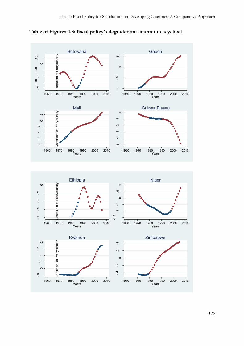
Chap4: Fiscal Policy for Stabilization in Developing Countries: A Comparative Approach
175
Table of Figures 4.3: fiscal policy’s degradation: counter to acyclical -.2
-.15
-.1-.0
5
0
.05
Coe
ffici
ent o
f Pro
cycl
ical
ity
1960 1970 1980 1990 2000 2010Years
Botswana
-1-.5
0.5
Coe
ffici
ent o
f Pro
cycl
ical
ity
1960 1970 1980 1990 2000 2010Years
Gabon
-8-6
-4-2
02
Coe
ffici
ent o
f Pro
cycl
ical
ity
1960 1970 1980 1990 2000 2010Years
Mali
-5-4
-3-2
-10
Coe
ffici
ent o
f Pro
cycl
ical
ity
1960 1970 1980 1990 2000 2010Years
Guinea Bissau
-.8-.6
-.4-.2
0
Coe
ffici
ent o
f Pro
cycl
ical
ity
1960 1970 1980 1990 2000 2010Years
Ethiopia
-1.5
-1-.5
0.5
1
Coe
ffici
ent o
f Pro
cycl
ical
ity
1960 1970 1980 1990 2000 2010Years
Niger
-.50
.51
1.5
2
Coe
ffici
ent o
f Pro
cycl
ical
ity
1960 1970 1980 1990 2000 2010Years
Rwanda
-.4-.2
0.2
.4
Coe
ffici
ent o
f Pro
cycl
ical
ity
1960 1970 1980 1990 2000 2010Years
Zimbabwe

Chap4: Fiscal Policy for Stabilization in Developing Countries: A Comparative Approach
176
fluctuations in the business cycle (Table of Figure 4.4). But the year 2001 inaugurates a
new era where policies were strongly procyclical. Sudan presents a similar situation where
things changed deeply. At this point one cannot help but wonder if a procyclical fiscal
policy is absolutely and everywhere always negative? Indeed in the Sudanese case (or
Lesotho) would it not be possible for these governments to run procyclical policies in
periods of economic prosperity to strengthen economic growth? This question of
whether procyclical fiscal policies are harmful or not to growth will be addressed in the
second stage of analysis of this paper.
Table of Figures4.4: fiscal policy’s degradation: counter to acyclical
01
23
4
Coeff
icien
t of P
rocy
clica
lity
1960 1970 1980 1990 2000 2010Years
Lesotho
-.50
.51
1.52
Coeff
icien
t of P
rocy
clica
lity
1960 1970 1980 1990 2000 2010Years
Sudan
Presented are some of the results from our dataset of 45 Sub-Saharan African countries.
Now I will be investigating the procyclicality of other fiscal variables such as government
investment and government consumption. This will allow us to see in detail which part of
government expenses is more pro or countercyclical.

Chap4: Fiscal Policy for Stabilization in Developing Countries: A Comparative Approach
177
4.4.4 The Government Investment
Public investments variable used here is the general government GDFI in constant
USD. The first set of diagrams shows some countries which initially began with
countercyclical public investments but ended with strong procyclical policies. For instance
in Algeria, Morocco and Burundi where public investment ends up being positively
related to business cycles. A possible explanation for this behaviour could be that the
period immediately after 1960 was characterized by “compulsory” investments whatever
the economic cycle (good or bad), since countries needed to build up. Thereafter, and
when the “necessary” public goods were provided, public authorities started purchasing
investment goods only when a financial windfall occurred.
For other economies (Tables of Figures 4.5) also, the situation changes toward more
procyclical investment policies. For Central Africa, Egypt, Gambia and Togo the data
shows insensitivity at the beginning and strong procyclical investments in recent years.
Other governments (Tanzania, Gabon, Ghana and Kenya) have almost constantly
pursued procyclical investment policies.
In Table of Figures 4.6, the results presented show countries with better policies, in other
words, strong countercyclical behaviour for public investments. Indeed, in Benin, Guinea-
Bissau and South Africa, investment seems to be used by authorities very “wisely”. But if
one looks more closely, the data shows that for Guinea Bissau (mainly) and Benin, during
relative long periods, the output gap was negative (GDP growth under its potential level)
and public authorities, in order to avoid the collapse of the economy, tried to keep a
certain level of basic spending in capital formation. For South-Africa, an emerging
country, this behaviour does not seem very surprising since from the data one can argue
that investment has been a stabilizing tool used to bail out the economy in bad times and
reduced during booms.

Chap4: Fiscal Policy for Stabilization in Developing Countries: A Comparative Approach
178
Table of Figures4.5: Procyclicality of Government Investment -.0
4-.0
2
0
.02
.04
.06
Coef
ficie
nt o
f Pro
cycli
cality
1960 1970 1980 1990 2000 2010Years
Algeria
-.03
-.02
-.01
0
.01
Coef
ficie
nt o
f Pro
cycli
cality
1960 1970 1980 1990 2000 2010Years
Burundi
-.01
-.008
-.006
-.004
-.002
0
Coef
ficie
nt o
f Pro
cycli
cality
1960 1970 1980 1990 2000 2010Years
Cote d'Ivoire
-.002
-.001
0
.001
.002
Coef
ficie
nt o
f Pro
cycli
cality
1960 1970 1980 1990 2000 2010Years
Morocco
-.004
-.002
0
.002
.004
Coef
ficie
nt o
f Pro
cycli
cality
1960 1970 1980 1990 2000 2010Years
Senegal
.003
4.003
45 .003
5.003
55 .003
6.003
65
Coe
ffici
ent o
f Pro
cycl
ical
ity
1960 1970 1980 1990 2000 2010Years
Central Africa
-.02-.0
15-.0
1-.005
0
.005
Coe
ffici
ent o
f Pro
cycl
ical
ity
1960 1970 1980 1990 2000 2010Years
Egypt
-.01
0
.01
.02
.03
Coe
ffici
ent o
f Pro
cycl
ical
ity
1960 1970 1980 1990 2000 2010Years
Gambia
-.006
-.004
-.002
0
.002
.004
Coe
ffici
ent o
f Pro
cycl
ical
ity
1960 1970 1980 1990 2000 2010Years
Togo

Chap4: Fiscal Policy for Stabilization in Developing Countries: A Comparative Approach
179
Table of Figures4.5: Procyclicality of Government Investment -.0
25-.0
2-.0
15-.0
1-.0
05
0
Coeff
icien
t of P
rocyc
licali
ty
1960 1970 1980 1990 2000 2010Years
Madagascar
-.005
0
.005
Coeff
icien
t of P
rocyc
licali
ty
1960 1970 1980 1990 2000 2010Years
Mauritius
0
.000
2.0
004
.000
6.0
008
Coe
ffici
ent o
f Pro
cycl
ical
ity
1960 1970 1980 1990 2000 2010Years
Gabon
.05
.1.1
5.2
.25
.3
Coe
ffici
ent o
f Pro
cycl
ical
ity
1960 1970 1980 1990 2000 2010Years
Ghana
.004
.006
.008
.01
.012
.014
Coe
ffici
ent o
f Pro
cycl
ical
ity
1960 1970 1980 1990 2000 2010Years
Kenya
.002
.004
.006
.008
Coe
ffici
ent o
f Pro
cycl
ical
ity
1960 1970 1980 1990 2000 2010Years
Tanzania

Chap4: Fiscal Policy for Stabilization in Developing Countries: A Comparative Approach
180
Table of Figures6: Procyclicality of Government Investment (usual countercyclical
countries).
-.001
6-.00
14-.0
012 -.0
01-.0
008
Coef
ficie
nt o
f Pro
cycli
calit
y
1960 1970 1980 1990 2000 2010Years
Benin
-.15
-.1-.0
5
0
Coef
ficie
nt o
f Pro
cycli
calit
y
1960 1970 1980 1990 2000 2010Years
Guinea Bissau
.004
.005
.006
.007
.008
Coef
ficie
nt o
f Pro
cycli
calit
y
1960 1970 1980 1990 2000 2010Years
South Africa
Next I will investigate the cyclical behaviour of general government final expenses
including purchases of goods and services, and compensation of employees.
4.4.5 The Government Consumption and Social Spending
As said above, here I will focus on government (non capital) spending cyclical
characteristics and run a comparison with results from public investment. However I
expect a higher countercyclicality from government non capital spending to investment.
Government consumption variables include purchases of goods and services,
compensation of public servants. Additional to that and based on IMF (2010), this
variable is called “pro-poor spending” because it incorporates expenses on health and
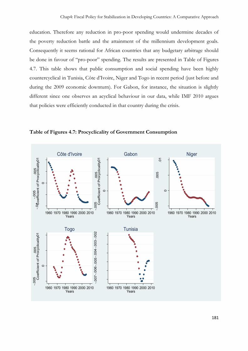
Chap4: Fiscal Policy for Stabilization in Developing Countries: A Comparative Approach
181
education. Therefore any reduction in pro-poor spending would undermine decades of
the poverty reduction battle and the attainment of the millennium development goals.
Consequently it seems rational for African countries that any budgetary arbitrage should
be done in favour of “pro-poor” spending. The results are presented in Table of Figures
4.7. This table shows that public consumption and social spending have been highly
countercyclical in Tunisia, Côte d‟Ivoire, Niger and Togo in recent period (just before and
during the 2009 economic downturn). For Gabon, for instance, the situation is slightly
different since one observes an acyclical behaviour in our data, while IMF 2010 argues
that policies were efficiently conducted in that country during the crisis.
Table of Figures 4.7: Procyclicality of Government Consumption
-.01
-.00
5
0
.005
.01
Coe
ffici
ent o
f Pro
cycl
ical
ity
1960 1970 1980 1990 2000 2010Years
Côte d'Ivoire
-.00
5
0
.005
.01
Coe
ffici
ent o
f Pro
cycl
ical
ity
1960 1970 1980 1990 2000 2010Years
Gabon-.
005
0
.005
.01
Coe
ffici
ent o
f Pro
cycl
ical
ity
1960 1970 1980 1990 2000 2010Years
Niger
-.00
5
0
.005
.01
Coe
ffici
ent o
f Pro
cycl
ical
ity
1960 1970 1980 1990 2000 2010Years
Togo
-.00
7-.
006
-.00
5-.
004
-.00
3-.
002
Coe
ffici
ent o
f Pro
cycl
ical
ity
1960 1970 1980 1990 2000 2010Years
Tunisia

Chap4: Fiscal Policy for Stabilization in Developing Countries: A Comparative Approach
182
More than half the total sample of countries previously pursuing procyclical public
consumption policies started in early 2000 implementing a new regime where
consumptions were at least disconnected from the business cycle (Table Figure A.4.1).
Table A.4.1 presents a comparison between public investment and consumption cyclical
walk for some countries. As IMF 2010 underlines, government expenditures have been
more countercyclical than public investment in the sample as a whole, but this picture
hides an important heterogeneity. The trend in recent years (from 2000) has shown that
the majority of middle income countries have run countercyclical public consumption or
at least things have been acyclical. Except for Algeria, all other middle-income economies
steadily evolve toward more acyclical then countercyclical public spending policies as in
the case of Botswana, Mauritius Egypt and South-Africa. On the investment side the
situation does not change for Algeria which still keeps a procyclical stance, and Egypt also
running the same policy. Apart from these two countries, South-Africa, Botswana and
Tunisia improved their investment policies. The picture is neither clear cut in low income
and fragile African states. However as a whole, the sample shows that public expenditures
(pro-poor spending) has been the main tool for African countries to fight recessions
during the 2000s. Only four countries (Algeria, Burundi, Guinea Bissau and Morocco) out
of twenty three have left spending moving in same direction as changes in output gap.
These results underline two important facts. First, the one “size fits all” from previous
studies is no longer relevant since substantial disparities exist among African economies.
Second, the general tendency is to run “wise” fiscal policies among African countries
(mainly for Sub-Saharan economies), therefore the situation described by Thornton
(2008) (where fiscal policies in developing countries were strongly procyclical and
inefficient to stabilize the economy) seems to have come to an end. International
Organizations such as IMF also share the same analysis arguing that, based on the latest
data available, fiscal policies during the crisis (in 2009) have indeed been countercyclical
and pro-poor spending has been protected. To a large extent, this reflects the stronger
fiscal positions in most countries heading into the crisis, and the availability of additional
external financing. The rising trend in health and education expenditures especially has
not been interrupted during the recent economic downturns. A growing number of

Chap4: Fiscal Policy for Stabilization in Developing Countries: A Comparative Approach
183
countries have put in place cash transfers, which have good targeting mechanisms and
typically offer high impact at low cost. And an increasing number of countries are taking a
more developmental approach to social protection, focusing on public works, and food
security, especially through agricultural input subsidies (IMF 2010).
The second part in this first stage analysis will focus on Latin American countries. Even if
their structures are quite different, this analysis will give a benchmark on the relative
performance between the groups of developing economies.

Chap4: Fiscal Policy for Stabilization in Developing Countries: A Comparative Approach
184
Table 4.1: Comparison for Sample Countries
Country Government Investment Public Consumption Algeria Procyclical Procyclical Botswana (previously procyclical) Acyclical Acyclical Benin Countercyclical Acyclical Burundi (previously countercyclical) procyclical Procyclical Cameroon Acyclical Acyclical Central African Republic Procyclical Côte d‟Ivoire (previously countercyclical) procyclical Countercyclical Egypt Procyclical Acyclical Gabon Procyclical Countercyclical Gambia Procyclical Procyclical then Acyclical Ghana Procyclical Procyclical then Acyclical Guinea Bissau Countercyclical Procyclical Kenya Procyclical Procyclical then Acyclical Madagascar Countercyclical then Acyclical Acyclical Mali Acyclical Acyclical Mauritius Countercyclical then Acyclical Acyclical Morocco Procyclical, Countercyclical then Procyclical Procyclical Niger Acyclical Countercyclical Senegal Procyclical then Acyclical Acyclical South Africa Countercyclical Acyclical Swaziland Acyclical Procyclical then Acyclical Tanzania Procyclical Acyclical Togo Procyclical Countercyclical Tunisia Procyclical then Acyclical Countercyclical

Chap4: Fiscal Policy for Stabilization in Developing Countries: A Comparative Approach
185
STUDY CASE 1: Procyclicality of Fiscal Policy in Senegal
The diagram below show that Senegalese budget balance have been quite countercyclical in
recent years, compared to the situation in the early 1960s until mid-1990s (if one considers
budget deficit, countercyclical policies appear more evidently during early 2000s) where public
spending (and the budget balance itself) simply followed the business cycle. This means that
policy makers are getting “fiscally wiser” Beyond the political economy arguments explaining
this change other possible reasons are more related to the change in international economic
orientations. Some details are given in flowing lines.
1 Senegalese government has learnt from the past: the late 1980s and mid-1990 (especially
in 1988 and 1994) have seen violent social unrests in the country. Of course there were
other causes than economic but the situation in the real economy played an important
role. For instance while the country was running poor economic performance in 1993,
with a negative output growth (around -2%), general government final consumption
expenditures declined. Therefore the procyclical public policies exacerbate the economic
downturn and feeded violent riots in the capital Dakar in February 1994.
2 Improved situation for public finance: had given enough room for Senegalese
government to steadily run less procyclical policies. Indeed with a lighter debt burden
(thanks to poverty relief programs) and favorable global economic environment,
government was able to improve its fiscal stance.
3 During 1980s policies implemented to sort out the country‟s debt crisis did give a little
attention to social sectors. Indeed while improving macroeconomic aggregates, structural
adjustment programs ended up with important negative social effects. That is what
poverty reduction programs are aimed at amending. Therefore, more recently, during
economic downturn (idiosyncratic or global crisis) the country receives financial as well
as “political” support from partners to keep at least social spending unchanged. That was
the situation during the last global crisis in 2008 when IMF & WB encouraged (and give
support) low income countries to keep unchanged “sensitive” spending.

Chap4: Fiscal Policy for Stabilization in Developing Countries: A Comparative Approach
186
Year 1990 1991 1992 1993 1994 1995 1996
General government final consumption expenditure (constant USD, billions)
0,54657173 0,53854874 0,5398254 0,53259239 0,51301194 0,51712061 0,52805213
GDP per capita growth (annual %)
3,4896325 -0,3100542 1,55171584 -1,46561308
2,72595116 2,5265245 -0,71984006
Year 1999 2000 2001 2002 2003 2004 2005 2006 2007
External Debt, total (FCFA, Billions)
2171,7 2418,9 2540,1 2294,9 2024,7 1864,6 1944,1 864,4 968,5

Chap4: Fiscal Policy for Stabilization in Developing Countries: A Comparative Approach
187
4.5 The Results from first step regressions: Latin American Countries
For sub-American economies the same method will be used, as in equation (1).
The adjusted primary deficit is also computed as in equation (2), and identical control
variables are introduced. The results are presented below.
Countries present in Set of Figures 4.8 (and 4.9) have undertaken good fiscal policy
responses during recessions. Bolivia, Uruguay, Costa Rica and El Salvador have indeed
steadily implemented countercyclical fiscal policies since discretionary fiscal actions go up
when actual output is significantly lower than its potential level. The greatest achievement
was performed by Honduras which pursued procyclical policies from 1971 to 1995 and
changed it all in 2000. Up to this point one important and trivial stylized fact is observed:
any change in the fiscal regime is preceded by a period where fiscal variables are
disconnected from output variations. Therefore one can reasonably imagine that
Argentina, Chile and Ecuador in coming years will have better fiscal policies, since they
seem to have given up procyclical responses to short term negative shocks on real
economy.
More interesting and more challenging results are shown in Set of Figures 4.10. Brazil,
Colombia, Peru and Venezuela have all been keeping strong procyclical fiscal policies
since the early 1990s (except for Peru). This situation is difficult to interpret because most
Latin American countries had very good fiscal positions from 2000 up to 2009. The
commodity prices boom in 2006-2007 contributed to improve the Latin American fiscal
balance (as much as economic cycles according to Daude & al. 2010). So that in 2008, at
the onset of the crisis, adjusted primary balances were in equilibrium or surplus in a
majority of countries; for instance there were surpluses in Peru, Brazil, Colombia,
Uruguay, and Costa-Rica. Despite this excellent fiscal shape, why do some of them run
procyclical policies? Several answers have been given in the literature. The first reason is
historical, indeed since early 1990s fiscal policy has been procyclical in many Latin
American countries (Argentina, Brazil, Costa-Rica, Mexico etc.). The procyclicality during
this period was mainly driven by the deep crises, but these practices continued throughout

Chap4: Fiscal Policy for Stabilization in Developing Countries: A Comparative Approach
188
the 2000s (De Mello & al. 2006), though countries like Costa-Rica, Honduras, El Salvador
and Uruguay ended this dynamic in the early 2000s.
Set of Figures 4.8: Adjusted fiscal deficit procyclicality
-.10
.1.2
.3.4
Coef
ficie
nt o
f Pro
cycli
cality
1960 1970 1980 1990 2000 2010Years
Bolivia-.4
-.3-.2
-.10
Coef
ficie
nt o
f Pro
cycli
cality
1960 1970 1980 1990 2000 2010Years
Costa Rica
-.3-.2
-.10
.1
Coef
ficie
nt o
f Pro
cycli
cality
1960 1970 1980 1990 2000 2010Years
El Salvador
-.05
0
.05
.1.1
5.2
Coef
ficie
nt o
f Pro
cycli
cality
1960 1970 1980 1990 2000 2010Years
Honduras
-.08
-.06
-.04
-.02
0
Coef
ficie
nt o
f Pro
cycli
cality
1960 1970 1980 1990 2000 2010Years
Uruguay

Chap4: Fiscal Policy for Stabilization in Developing Countries: A Comparative Approach
189
Set of Figures 4.9: Adjusted fiscal deficit procyclicality
-.3-.2
-.10
.1
Coef
ficien
t of P
rocy
clica
lity
1960 1970 1980 1990 2000 2010Years
Argentina
-.05
0
.05
.1
Coef
ficien
t of P
rocy
clica
lity
1960 1970 1980 1990 2000 2010Years
Chile
-.4-.2
0.2
.4
Coef
ficien
t of P
rocy
clica
lity
1960 1970 1980 1990 2000 2010Years
Ecuador
Set of figures 4.10: Adjusted fiscal deficit procyclicality
-.05
0
.05.1
.15.2
Coeff
icien
t of P
rocy
clica
lity
1960 1970 1980 1990 2000 2010Years
Brazil
-.04-
.02
0
.02.04
.06
Coeff
icien
t of P
rocy
clica
lity
1960 1970 1980 1990 2000 2010Years
Colombia
-.05
0
.05.1
Coeff
icien
t of P
rocy
clica
lity
1960 1970 1980 1990 2000 2010Years
Peru
0
.05.1
.15.2
Coeff
icien
t of P
rocy
clica
lity
1960 1970 1980 1990 2000 2010Years
Venezuela

Chap4: Fiscal Policy for Stabilization in Developing Countries: A Comparative Approach
190
Another explanation for such fiscal stance is the size of automatic stabilizers in Sub-
American economies. It is well known that with significant automatic stabilizers,
discretionary measures needed to stabilize the economy will be less important than in the
situation where one has weak automatic responses74. Therefore, important discretionary
measures are unnecessary since the automatic response of fiscal primary deficit is enough
to curb the recession. Additional to these facts, EMEs and especially Sub-American ones
were among the first to start recovering from recession, owing to current surplus, low
debt levels, strong monetary policies (inflation targeting), and important capital inflows
that helped prompt recovery.
As it was done for African countries, similar benchmark estimations for government
investment and government consumption will be made.
4.5.1 The Government Investment
Due to the nature of our database, the gross fixed capital formation will be used as
a proxy for public investments (in real US dollars).
On the investment side, Bolivia and Peru are characterized by a change, at the end of
1990s, in their investment policies, spending more in periods of economic downturn.
However in Brazil the investment policy after a long period of acyclicality has recently (in
2003) become quite countercyclical. In the remaining countries for which data on public
investment is available, the situation is split in two. In the Set of Figures 4.11, capital
spending is strongly procyclical especially for Uruguay and Costa-Rica. Venezuela, if one
refers to the stylized fact presented earlier, is engaging a new dynamic and I expect in the
medium term that this country will be using capital expenditures as a stabilizing tool. For
the remaining countries, presented in Table Figure A.4.2, investment is just not
responding to any change in output gap.
74 Primary budget balances have an automatic response of 0.21 percentage points of GDP for each output
gap in the region (Daude & al. 2010).

Chap4: Fiscal Policy for Stabilization in Developing Countries: A Comparative Approach
191
The next analysis will focus on the cyclical nature of government final consumption
expenditure.
Set of Figures 4.11: Procyclicality of government investment (strong
countercyclical)
-200
0-1
000
0
1000
Coe
ffici
ent o
f Pro
cycl
ical
ity
1960 1970 1980 1990 2000 2010Years
Bolivia
-4.0
0e+0
8-3
.00e
+08
-2.0
0e+0
8-1
.00e
+08 0
Coe
ffici
ent o
f Pro
cycl
ical
ity
1960 1970 1980 1990 2000 2010Years
Brazil
0
5000
010
0000
1500
00
Coe
ffici
ent o
f Pro
cycl
ical
ity
1960 1970 1980 1990 2000 2010Years
Peru

Chap4: Fiscal Policy for Stabilization in Developing Countries: A Comparative Approach
192
Set of Figures 4.11: Procyclicality of government investment (strong procyclical)
-.1-.0
5
0
.05.1
.15
Coeff
icien
t of P
rocy
clica
lity
1960 1970 1980 1990 2000 2010Years
Costa Rica
-.02
-.01
0
.01.02
Coeff
icien
t of P
rocy
clica
lity
1960 1970 1980 1990 2000 2010Years
Honduras
-100
-50
050
Coeff
icien
t of P
rocy
clica
lity
1960 1970 1980 1990 2000 2010Years
Uruguay
01
23
45
Coeff
icien
t of P
rocy
clica
lity
1960 1970 1980 1990 2000 2010Years
Venezuela
4.5.2 The Government consumption and social spending
General government final consumption expenditure (from WDI database) is used
here as a proxy for government. It includes all government current expenditures for
purchases of goods and services (including compensation of employees). It also includes
most expenditure on national defence and security, but excludes government military
expenditures that are part of government capital formation.
Some Latin American countries are characterized by relatively strong countercyclical
public consumption. Indeed Brazil, Bolivia, Chile, Costa-Rica, Panama and Venezuela
governments use their consumption as a stabilizing tool (Set of Figures 4.12). Further
analysis is necessary in order to explain why there seems to be a contradiction between
public consumption and the procyclical nature of fiscal deficit. But as said earlier,
automatic stabilizers are very effective in these economies. Moreover, and according to
Daude & al. 2010, personal income taxes, without any discretionary action, are highly
responsive to change in output gap. Therefore, despite a countercyclical use of

Chap4: Fiscal Policy for Stabilization in Developing Countries: A Comparative Approach
193
government spending in some countries, the automatic stabilizers effects seem to have
higher effects on real economy than discretionary measures.
Other countries, in Table Figure A.4.3, present acyclical or procyclical public
consumption policies in recent periods (late 1990s).
A brief comparison between Latin American and African countries shows that the latter
are increasingly implementing countercyclical fiscal policies while budget deficit is more
procyclical in developing Latin America. The two different behaviours can be easily
explained by the tax bases. Indeed Sub-American countries (e.g. Brazil) have a relative
wider personal income tax base compared to African countries (especially Sub-Saharan
ones) where tax collection is more challenging and relies on fewer contributors. Therefore
the only way to significantly stabilize the economic activity would be through
discretionary fiscal actions. Inversely for small recessions, Latin American countries might
only let automatic movements of taxes regulate the economic activity.

Chap4: Fiscal Policy for Stabilization in Developing Countries: A Comparative Approach
194
Set of Figures 4.12: Procyclicality of government investment (countercyclical) -.
20
.2.4
Co
eff
icie
nt
of
Pro
cyclic
alit
y
1960 1970 1980 1990 2000 2010Years
Bolivia
-.1
0.1
.2
Co
eff
icie
nt
of
Pro
cyclic
alit
y
1960 1970 1980 1990 2000 2010Years
Brazil
-.1
2 -.1-.
08-.
06-.0
4-.0
2
Co
eff
icie
nt
of
Pro
cyclic
alit
y1960 1970 1980 1990 2000 2010
Years
Chile
-.6
-.4
-.2
0
Co
eff
icie
nt
of
Pro
cyclic
alit
y
1960 1970 1980 1990 2000 2010Years
Costa Rica
-.3
-.2
-.1
0.1
Co
eff
icie
nt
of
Pro
cyclic
alit
y
1960 1970 1980 1990 2000 2010Years
Honduras
-.2
-.1
0.1
Co
eff
icie
nt
of
Pro
cyclic
alit
y
1960 1970 1980 1990 2000 2010Years
Panama
-.1
-.0
8-.0
6-.0
4-.0
2
Co
eff
icie
nt
of
Pro
cyclic
alit
y
1960 1970 1980 1990 2000 2010Years
Venezuela
Chap4: Fiscal Policy for Stabilization in Developing Countries: A Comparative Approach
195
4.6 Second Stage Regression: Is Procyclicality of Fiscal
Policy always and everywhere bad?
In this section I cover an area that has not been dealt with for developing countries and
in which the question is raised as to whether procyclical fiscal policies are bad for economic
activity, always and everywhere. It is imaginable that a government decides to run procyclical
fiscal policies in periods of economic bonanza in order to support and strengthen GDP
growth. On the other hand, as fully explained in the literature, procyclical fiscal policy
increases the vulnerability toward shocks since public authorities will not have enough
financial resources to cover loss of tax revenues or even increase its spending to support
inactivity during recessions. To shed light on such possible effects, I regress a measure for
GDP volatility on output gap coefficients from earlier time series estimations (called
“coefficients of procyclicality). If there is a clear positive effect of coefficients of
procyclicality on output volatility, one could be able to conclude at least that procyclical fiscal
policy induces higher volatility for growth and this could discourage private entrepreneurship
and investment.
Aghion & Marinescu (2007) did a similar analysis on OECD countries but they used first
difference of the log of real GDP per capita. For developing economies, it might be more
relevant to use output volatility since these countries are more vulnerable to volatility (Loayza
& al. 2007). As Loayza & al. (2007) underline, “volatility entails a direct welfare cost for risk-
averse individuals, as well as an indirect one through its adverse effect on income growth and
development”.

Chap4: Fiscal Policy for Stabilization in Developing Countries: A Comparative Approach
196
4.6.1 Empirical Specification and Results
The empirical specification is as follow:
2 1 3( ) varit it it itVariance Y control
The dependent variable is the variance of real output. 1it is the coefficients obtained from
first stage estimation and they are compiled to form a panel dataset. varitcontrol is a set of
control variables that are introduced. Current account balance is still here to control for
possible current account targeting, inflation, lagged GDP and investment over GDP are also
considered.
4.6.1.1 The results from African countries database
Table 4.13 column-1 presents the results from a simple OLS estimation with a set of
control variables representing the most widely used in similar analysis (e.g. Aghion &
Marinescu 2007). Also I use country-year fixed effects in order to control for specific
characteristics for each country even if they share similar levels of development or are in the
same region. One observes here that the positive and statistically significant relationship
between the coefficients of procyclicality and output volatility suggests that countercyclical
fiscal deficit is an efficient stabilizing tool. Indeed countercyclical fiscal deficit impacts
positively on growth (here it reduces its volatility) in that it can help reduce the negative
effect that negative liquidity shocks impose on credit-constrained firms that invest in R&D
and innovation (Aghion & Marinescu 2007).
The sign of other control variables are as expected. For instance, better current account
balance is growth enhancing and reduces volatility. Inflation and the lagged output also are as
expected. However this first estimation might suffer from an endogeneity bias with output

Chap4: Fiscal Policy for Stabilization in Developing Countries: A Comparative Approach
197
growth that could affect the cyclical coefficient and vice-versa. Furthermore, the lagged value
for real GDP per capita might be endogenous and correlated to the error term.
To address such possible source of bias I will use the GMM system method which allows us
to control for possible endogeneity bias by using lagged values as instruments. Results are
presented in Table 4.13 column-2. Despite our concerns about possible endogeneity the
results are quite trustworthy compared to those of OLS.
Table 4.13: Effects of Fiscal policy procyclicality on Growth volatility
FE GMM System
VARIABLES variance variance
cdeficit_acycygap 0.145** 0.168**
(0.0634) (0.0752)
curr_acc_real -2.06e-06 -1.10e-06**
(8.89e-06) (4.33e-07)
inflation 0.00133** 0.00169***
(0.000615) (0.000398)
lag_gdp 0.000855*** -0.000284***
(9.45e-05) (1.59e-05)
invest -1.75e-06 -1.97e-06***
(1.15e-05) (4.10e-07)
gdp_cap_real 0.00120***
(3.17e-05)
Constant 37.56*** 37.36***
(0.131) (0.0952)
Observations 740 740
R-squared 0.112
Number of fixed_id_year 33
Number of id 37
Standard errors in parentheses
*** p<0.01, ** p<0.05, * p<0.1

Chap4: Fiscal Policy for Stabilization in Developing Countries: A Comparative Approach
198
Procyclical fiscal policy still negatively and statistically significantly affects growth through
higher volatility. This shows that the endogeneity issue did not affect our results that much.
The second step of estimation is also done for Latin American countries to see whether the
impact is the same as for African economies.
4.6.1.2 Effects of Fiscal Procyclicality for Latin American Countries
Results from OLS estimations on Table 4.14 column1 denote that more procyclical fiscal
policy induces higher output volatility in developing South-American countries. When
discretionary fiscal measures are considered alone, it is quite logical to obtain such negative
impact on growth, but if linked to previous analysis the impact might not be that large.
Indeed, automatic stabilizers are said to be relatively important in Latin American countries,
therefore the real effect of procyclical discretionary measures on output volatility will be less
important. When we move from column-1 to column-2 (from an OLS to a GMM estimation
where I check for possible endogeneity of the coefficient of procyclicality), the variable of
interest becomes statistically significant only at 10%, where it was at 5% in the OLS
estimations. Also one has to notice that, despite a very small coefficient, current account
balance positively impacts on output volatility. Compared to results for African economies
this is a bit remarkable. Improvement of current account balance should mean that the
economy becomes more competitive and production should increase and remain stable. But
for Latin American countries, this result might be explained by the repetitive crises caused by
unsustainable current account balance and speculative capital inflows (refer to chapter 2).
Therefore, an increase in current account balance is “always” perceived by our data as a
possible sign for potential future crisis especially for developing countries running a non-
flexible exchange rate policy75.
75 Recently, during the autumn of 2009, Brazil decided to control capital inflows since it was running a higher
current account balance and faced important capital inflows. Therefore to avoid real appreciation of the

Chap4: Fiscal Policy for Stabilization in Developing Countries: A Comparative Approach
199
Table 4.14: Effects of Fiscal policy procyclicality on Growth volatility
(1) (2)
VARIABLES variance variance
L.variance 0.971***
(0.0158)
Coefficient of Procyclicality 1.914** 1.393*
(0.807) (0.655)
curr_acc_real 1.24e-07 1.91e-07***
(4.92e-07) (3.78e-08)
lag_gdp 0*** -0***
(0) (0)
invest -2.21e-07 -2.69e-07***
(1.44e-07) (6.75e-08)
gdp_cap 0***
(0)
inflation 0.000221 -6.30e-06
(0.000192) (5.63e-05)
durable -8.56e-05
(0.000259)
Constant 42.11*** 1.306*
(0.138) (0.673)
Observations 447 447
R-squared 0.073
Number of fixed_id_year 38
Number of id 15
Standard errors in parentheses *** p<0.01, ** p<0.05, * p<0.1
Brazilian Real and reduce vulnerability toward external shocks, public authorities introduced a tax of around
10% on portfolio investments.

Chap4: Fiscal Policy for Stabilization in Developing Countries: A Comparative Approach
200
4.7 Conclusion
A new preference in developing countries for less procyclical fiscal policies and more
active and countercyclical budget measures is becoming apparent. For instance, most African
countries have generally been using the budget deficit to stabilize their economies. Except for
a few “outliers” (Rwanda, Sudan), countries are moving toward more countercyclical policies
from either initially procyclical policies (Algeria, Central African Republic, Egypt etc.) or
acyclical budget deficits (Cameroon, Ghana, Togo, Tunisia, Senegal etc.). The comparison
between investment and public consumption shows that pro-poor spending has been more
countercyclical. Indeed African economies, especially during the last global economic
downturn, made all possible efforts to keep social expenditures unchanged or even increase
them, as IMF (2010) reported it. This indicates a growing trend where developing African
countries learn from previous painful experience when they were obliged to run restrictive
fiscal policies in periods of negative output gap. The situation in other developing countries
is quite similar but some differences remain.
Indeed large countries such as Brazil (as well as Colombia, Peru and Venezuela) were
surprisingly running procyclical budget deficits. With responsive and large automatic
stabilizers in these economies, lesser discretionary measures needed during recessions (or
even procyclical fiscal policies can be run without any danger if automatic stabilizers are large
enough). Other countries have been running (since the late 1990s) strong countercyclical
fiscal policies (Bolivia, Costa-Rica, El Salvador, Honduras and Uruguay).
Developing countries should deploy all possible efforts to implement rigorous policies with
their budget since it appears to be a strong factor for output stability. For developing African
countries, procyclical fiscal policies have been associated with strong volatility of output
while for Latin America this is still true but with a weaker significance.

Chap4: Fiscal Policy for Stabilization in Developing Countries: A Comparative Approach
201
Overall the paper demonstrates that for middle income and low income countries there is a
trend toward countercyclical policies since the results show that it is an efficient tool to
stabilize the real economy.
Despite such outcomes, fiscal policy alone is not enough to stabilize a whole economy. In
addition, discretionary fiscal measures should be consistent with monetary policy stance. For
instance, if in periods of recession government needs to borrow in order to support the
economy, authorities should run loose monetary policy to make funds available for
entrepreneurs and increase external competitiveness.
For a better efficiency, discretionary fiscal measures could be institutionalized similar to what
is being done in the monetary policy area. Similar to inflation targeting rules, implementing a
law regarding discretionary fiscal measures could strengthen the credibility of public
authorities and increase budget efficiency. Even for countries with fiscal rules, discretionary
measures still need to be clearly agreed upstream to avoid any rigidities. As the Ter-
Minassian (2010) survey points out, “half of countries operating under fiscal rules did not
modify or temporarily suspend them during the global crisis in 2008”. This discretionary
fiscal policy rule could also be a rampart against any deficit bias if it allows the measure to be
implemented as soon as the output gap reaches a certain negative value.

Chap4: Fiscal Policy for Stabilization in Developing Countries: A Comparative Approach
202
ANNEXES CHAPTER 4

Chap4: Fiscal Policy for Stabilization in Developing Countries: A Comparative Approach
203
Table Figure A.4.1 : Procyclicality of Government consumption (sample of African
Economies) 0.0
05.0
1.015
.02
Coe
ffici
ent o
f Pro
cycl
ical
ity
1960 1970 1980 1990 2000 2010Years
Botswana
-.004-.
002 0
.002.
004
Coe
ffici
ent o
f Pro
cycl
ical
ity
1960 1970 1980 1990 2000 2010Years
Cameroon
-.002
0
.002.
004.0
06
Coe
ffici
ent o
f Pro
cycl
ical
ity
1960 1970 1980 1990 2000 2010Years
Ethiopia
0
.02.
04.0
6.08
Coe
ffici
ent o
f Pro
cycl
ical
ity
1960 1970 1980 1990 2000 2010Years
Kenya-.1
5 -.1-.0
5 0
.05 .1
Coe
ffici
ent o
f Pro
cycl
ical
ity
1960 1970 1980 1990 2000 2010Years
Madagascar
-.005
0.005
.01.0
15
Coe
ffici
ent o
f Pro
cycl
ical
ity
1960 1970 1980 1990 2000 2010Years
Mauritius
-.005
0
.005
.01
Coe
ffici
ent o
f Pro
cycl
ical
ity
1960 1970 1980 1990 2000 2010Years
Senegal
-.01
0
.01
.02
Coe
ffici
ent o
f Pro
cycl
ical
ity
1960 1970 1980 1990 2000 2010Years
South Africa
0.01.0
2.03.0
4.05
Coe
ffici
ent o
f Pro
cycl
ical
ity
1960 1970 1980 1990 2000 2010Years
Swaziland
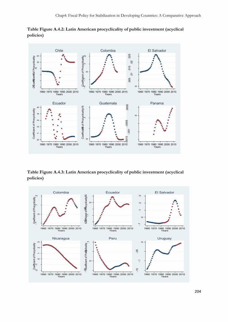
Chap4: Fiscal Policy for Stabilization in Developing Countries: A Comparative Approach
204
Table Figure A.4.2: Latin American procyclicality of public investment (acyclical
policies) -2
0-1
5-1
0-5
05
Coe
ffici
ent o
f Pro
cycl
ical
ity
1960 1970 1980 1990 2000 2010Years
Chile
-.2-.1
0.1
.2
Coe
ffici
ent o
f Pro
cycl
ical
ity
1960 1970 1980 1990 2000 2010Years
Colombia
0
.005
.01
.015
.02
.025
Coe
ffici
ent o
f Pro
cycl
ical
ity
1960 1970 1980 1990 2000 2010Years
El Salvador
01
23
45
Coe
ffici
ent o
f Pro
cycl
ical
ity
1960 1970 1980 1990 2000 2010Years
Ecuador
0
.05
.1.1
5
Coe
ffici
ent o
f Pro
cycl
ical
ity
1960 1970 1980 1990 2000 2010Years
Guatemala
-.001
5-.0
01-.0
005
0
.000
5
Coe
ffici
ent o
f Pro
cycl
ical
ity
1960 1970 1980 1990 2000 2010Years
Panama
Table Figure A.4.3: Latin American procyclicality of public investment (acyclical
policies)
-.10
.1.2
Coef
ficien
t of P
rocy
clica
lity
1960 1970 1980 1990 2000 2010Years
Colombia
-.15
-.1-.0
5
0
.05
Coef
ficien
t of P
rocy
clica
lity
1960 1970 1980 1990 2000 2010Years
Ecuador
-.10
.1.2
.3
Coef
ficien
t of P
rocy
clica
lity
1960 1970 1980 1990 2000 2010Years
El Salvador
-2-1
01
23
Coef
ficien
t of P
rocy
clica
lity
1960 1970 1980 1990 2000 2010Years
Nicaragua
-.05
0
.05
.1
Coef
ficien
t of P
rocy
clica
lity
1960 1970 1980 1990 2000 2010Years
Peru
-.15
-.1-.0
5
0
Coef
ficien
t of P
rocy
clica
lity
1960 1970 1980 1990 2000 2010Years
Uruguay

Chap4: Fiscal Policy for Stabilization in Developing Countries: A Comparative Approach
205
List of variables
Variable Definition & Source
Government investment General government gross domestic
investment (GDFI): i.e. gross fixed
capital formation including all
additions to the stocks of fixed
assets (purchases and own-account
capital formation), less any sales of
second-hand and scrapped fixed
assets, by central government.
Source: World Bank
Government consumption
and social spending
General government consumption
including all government current
expenditures for purchases of goods
and services (including
compensation of employees). It also
includes most expenditures on
national defense and security, but
excludes government military
expenditures that are part of
government capital formation.
Source: World
General Government debt External debt: consists of the
outstanding stock or recognized,
direct liabilities of the government
to the rest of the world, generated in
the past and scheduled to be
extinguished by government
operations in the future or to
continue as perpetual debt.
Source: World Bank
Inflation Annual percentage change of the
consumer price index
Source: IFS-IMF
GDP_growth Annual percentage growth rate of
GDP per capita.
Source: World Bank national
accounts data.
Current account balance The sum of net exports of goods,
services, net income, and net current
transfers. Source: BOP-Stats, IMF
& World Bank.

Chap4: Fiscal Policy for Stabilization in Developing Countries: A Comparative Approach
206
List of countries
AFRICA
LATIN AMERICA
Algeria Malawi Argentina
Angola Mali Belize
Benin Mauritania Bolivia
Botswana Mauritius Brazil
Burkina Faso Morocco Chile
Burundi Mozambique Colombia
Cameroon Namibia Costa Rica
Cape Verde Niger Ecuador
Central Africa Nigeria El Salvador
Chad RDC Guatemala
Comoros Rwanda Honduras
Congo Sao tome and principe Nicaragua
Cote d'Ivoire Senegal Panama
Djibouti South Africa Peru
Egypt Sudan Suriname
Equatorial Guinea Swaziland Uruguay
Eritrea Tanzania Venezuela
Ethiopia Togo Gabon Tunisia Gambia Zambia Ghana Zimbabwe Guinea
Guinea Bissau Kenya Lesotho Madagascar

General Conclusion
207

General Conclusion
208
General Conclusion

General Conclusion
209
General Conclusion
In a global context of instability and scarcity of external financial resources tax
revenues and public spending strategies needs to be highly efficient and effective in order
to keep a sustained path of economic development. This dissertation discussed the effects
of fiscal policies through three issues among the most important elements one has to
understand in order to improve this political economy tool. The literature on fiscal
policies in developing countries, for both emerging and low income economies, have
often neglected several essential specificities while identifying some phenomenon and/or
even considered that developing countries did not adapt their policies from past (crises)
experiences. The current dissertation tried to shed light on fiscal policies effects by
answering three questions and providing with policy recommendations: can developing
countries reasonably use surprise policies to improve economic activity? In a globalized
world, are the fiscal policies of developing economies‟ partners a real threat to the access
to private funds? Finally can fiscal policy be an efficient economic stabilizing tool?
The second chapter relies on a recent econometric technique to clearly identify the
outcome from a new policy that agents in the economy did not know about. The results
have shown that spending shocks have Keynesian effects, meaning that it has influenced
positively private consumption and output growth. On the other hand sudden change in
government revenues implies non-Keynesian effects since both consumption (and
imports) and growth increase. The results of spending shock are common to major
studies but those concerning public revenues shocks are quite surprising and deserve
deeper analysis. Several factors contribute to the non-Keynesian effects of public
revenues shocks. First, these results regarding public revenues, simply confirm that the
public sector is the main economic agent and also private sector is under-developed. The
lack of a strong private sector partially explains the fact whenever public revenues
increase absorption follows an identical path; the general state being the main employer in
the formal sector. The second factor identified is the weakness of automatic stabilizers in

General Conclusion
210
developing countries. This weakness is reflected through the fact that impulse responses
of revenue shocks last quite long (compare to what is observed in industrial countries).
This duration demonstrates that revenues are not flexible indicating the incapacity for
government to re-adapt its fiscal policy to changes in the real economy. The final factor is
related to the lack of credibility of public authorities. This causes behavioural strategies
such as “voracity effects” obliging government to spend any revenue “windfall”. All these
effects teach us that developing countries have reached “equilibrium state” where agents
do not trust their public authorities and these policy makers being aware of that adapt
their behaviour in order to appear less suspicious. The overall outcome being the fact that
fiscal policy in developing countries remains “unconventional”.
Chapter 3 had analyzed the relation between fiscal policies in both industrial and
emerging economies and the access to international private capital for these fast growing
emerging countries. The early stages of the recent global economic crisis in 2008 have
seen capital outflow from emerging economies. Indeed a “global crowding out”
consisting in capital flows being attracted by industrial countries‟ governments in huge
need of capital. Developing countries‟ fiscal imbalances also plays negatively against
capital inflows. This chapter‟s results confirm and also complete previous findings stating
that “push factors” (see supra) are the most important determinants for capital flows.
Henceforth among the “push factors” one will need to include the fiscal stance in
advanced countries as a key determinant of investment flows toward the developing
world. The non-linear relationship discovered between capital flows and fiscal imbalances
in industrial countries shows up that above a certain level of debt and deficit investment
flows to developing countries enter into a new paradigm. A country, whatever its level of
development, cannot indefinitely keeps large fiscal deficits (and debt) without raising
investors‟ concern. The recent situation in several European member countries (Greece,
Spain, Ireland and recently Portugal) constitutes an important evidence proving that fiscal
sustainability is not a unique matter for non-industrialized economies.
As extensively stated in previous analysis, fiscal policy in developing countries (African
and Latin American countries) have remained procyclical across decades (Chapter 4). It
has been true that fiscal policies were imprudent and even in some situation (especially

General Conclusion
211
during the late 1980s where strict restrictive fiscal policies were advocated) these policies
exacerbate the cyclical crises. However since early 2000 several developing countries
(African and Latin-American) learnt from past and “painful” experience. Progressively
many of them started shifting toward more prudent fiscal policies. This change will
provide them with enough “budget space” in terms of resources to support the real
economy in case their countries face severe economic downturn. Nonetheless developing
countries are at the early stages of this transition, since only a limited number of them
actually start implementing countercyclical policies. The other group of countries is still
on the medium stage where fiscal policy is rather acyclical. Another aspect of this
transition period is that countries running countercyclical policies use spending on social
sector (and not that much on investment) as the main stabilizing tool. These new
“disciplined policies” have to be encouraged and backed, otherwise a return toward
procyclical strategies might be a serious threat on the poverty alleviation objective and on
the whole economic development process (as the result suggest that procyclical policies
increase output volatility).
This dissertation has shown that fiscal policies in developing countries suffer from a lack
of credibility and a weak trust relationship between policy makers and tax payers, these
situations ending with severe inefficiencies. Deep reforms on institutional framework and
implementation of clear rules will help to mitigate these adverse effects. For instance and
like India did recently in 2003, that implemented a fiscal rule policy, is a possible way
other countries could explore. However while implementing fiscal rules one should care
about flexibility in order to avoid situations where the economy needs a stimulus and the
law prevents authorities to do so. Recent initiatives like PEMFA and MTEF are part of
this framework that aims at strengthening fiscal institution; and future research may
evaluate their real impact in developing countries‟ policies.
Another aspect of this dissertation has proved that despite the low efficiency of
government budgetary interventions things are changing and getting better in the
developing world. Even if industrial countries are their main competitors for the access to
capital, the results show a new tendency and a birth of a new paradigm. Developing
countries (EMEs) running sounder fiscal policies and growing at the faster rate seems to

General Conclusion
212
reverse the traditional situation and to be perceived as safer shelter by international
investors. On the same vein, and contrary to the common view, developing countries
have learnt a lot from the past. Fiscal policies are getting more disciplined and flexible
across countries.
To be sustainable all these great achievement alone are not enough to the ultimate
development objectives. Private sector and private savings strengthening are some of the
key element essential to lighten the fiscal efforts necessary to stabilize the macroeconomic
environment.

References
213
References
Chapter1:
Azam, J.-P., 2001. Macroeconomic Reforms in the CFA Franc Zone. Chap. 11 in ELBADAWI I. &
B. NDULU (eds.), Economic Development in SubSaharan Africa, Palgrave, Houndmills, NY.
Baldacci, E., Clements, B., Granados, C. M., Gupta, S., 2005. Fiscal policy, expenditure composition, and
growth in low-income countries. Journal of International Money and Finance, vol. 24, pp. 441-
463.
Barro, R., 1974. Are government bonds net wealth? Journal of Political Economy, Vol. 82, No. 6.
Bean, C., Buiter, W., 1987. The plain man‟s guide to fiscal and financial policy. London: Employment
Institute.
Benhabib, J., Schmitt-Grohe, S., Uribe, M., 2001. The Perils of Tylor Rules. Journal of Economic Theory
No.96, pp. 40–69.
Bernheim, D., 1989. A neoclassical perspective on budget deficits. Journal of Economic Perspectives,
Vol. 3.
Blanchard, O., 1990. Suggestions for a New set of fiscal indicators. OECD Economic Department
Working Paper 79.
Block, S., 2002. Elections, electoral competitiveness, and political budget cycles in developing countries.
Harvard University Working Paper No.78. Cambridge MA.
Bouakez, H., Chihi, F., Normandin, M., 2010. Measuring the Effects of Fiscal Policy. CIRPEE Working
Paper No.10-16.
Brender, A., Drazen, A., 2005. Political budget cycles in new versus established democracies. Journal of
Monetary Economics 52, 1271–1295.
Brun, J-F., Chambas, G., Combes, J-L., 2006. Recettes publiques des pays en développement Méthode
d‟évaluation. CERDI Working Papers No. 200611.
Brun, J-F., Chambas,G., Laporte, B., 1999. Financement externe et politique budgétaire : le rôle du
STABEX. Tiers-Monde, tome 40 No. 160, pp. 775–787.

References
214
Buiter, W., 1985. A guide to public sector debt and deficits. Economic Policy, vol. 1 pp. 13–79.
Calderon, C.A., Chong, A., Loayza N.V., 2002. Determinants of Current Account Deficits in Developing
Countries. World Bank Policy Research Paper No.2398.
Carmignani, F., 2010. Cyclical fiscal policy in Africa. Journal of Policy Modeling No.32, pp.254–267.
Chambas, G., 2010. Mobiliser des ressources locales en Afrique subsaharienne. ed. Economica
Chambas, G., 2005, Afrique au Sud du Sahara. Mobiliser des ressources fiscales pour le développement.
Economica, Paris.
Chichi, F., Normandin, M., 2008. External and Budget Deficits in Developing Countries. CIRPE
Working Paper No.08-19.
Chinn, M.D., Prasad, E.S, 2003. Medium-Term Determinants of Current Accounts in Industrial and
Developing Countries: An Empirical Exploration. Journal of International Economics No.59,
pp. 47–76.
Collier, P., Gunning, J.W., 1999. Trade Shocks in Developing Countries. Oxford University Press, Vol. 1.
Combes, J-L., Saadi-Sedik, T., 2006. How does trade openness influence budget deficits in developing
countries? The Journal of Development Studies, Vol. 42 No.8, pp. 140 –1416.
Daniel, B.C., 2007. The fiscal theory of the price level and initial government debt. Review of Economic
Dynamics No.10, pp. 193–206.
De Piniés, J., 1989. Debt sustainability and overadjustment. World Development Vol. 17 No.1 pp. 29–
43.
Favero, C.A., Giavazzi, F., 2002. Inflation Targeting and Debt: Lessons from Brazil," NBER Working
Papers No. 10390.
Giavazzi, F., Pagano, M., 1990. Can severe fiscal contractions be expansionary? Tales of two small
European countries. NBER Macroeconomics Annual.
Giavazzi, F., Pagano, M., 1996. Non keynesian effects of fiscal policy changes: International Evidence and
the Swedish experience. Swedish Economic Policy Review, n°3, pp. 69–103.
Haavelmo, T., 1954. A study in the theory of economic evolution. Amsterdam: North Holland.
Hansen B., 1999. Threshold effects in non-dynamic panels: estimation, testing and inference. Journal of
Econometrics, vol. 93, pp. 345-368.

References
215
Horne, J., 1991. Indicators of Fiscal Sustainability. IMF working paper 91/5.
IMF, 2009. The Case for Global Fiscal Stimulus. Staff Policy Notes No. 09/03.
Landais, B., 1998. Leçons de Politique Budgétaire. in ed. De Boeck, collection Ouvertures économiques.
Leeper, E. M., 1991. Equilibria under „Active‟ and „Passive‟ Monetary and Fiscal Policies. Journal of
Monetary Economics No.27.
Le-Houerou, P., Taliercio, R., 2002. Medium Term Expenditure Frameworks: From Concept to Practice.
Africa Region Working Paper Series No. 28.
Moisseron, J.-Y., Raffinot, M., 1999. Dette et pauvreté, Solvabilité et allégement de la dette des pays à
faible revenu. Economica, Paris.
Nordhaus, W., 1975. The political business cycle. Review of Economic Studies No. 42, pp. 169–190.
Özbilgin, H.M., 2010. Financial market participation and the developing country business cycle. Journal of
Development Economics Vol. 92, Issue 2, pp. 125–137.
Pattillo, C., Poirson, H., Ricci, L., 2002. External Debt and Growth. IMF Working Paper, No.69.
Pressman, S., 1997. Consumption, Income Distribution and Taxation: Keynes‟ Fiscal Policy. Journal of
Income Distribution vol. 7, pp. 29–44.
Rogoff, K., 1990. Equilibrium political budget cycles. American Economic Review No.80, pp. 21–36.
Schuknecht, L., 1996. Political business cycles and fiscal policies in developing countries. Kyklos 49, 155–
170.
Seater, J., 1993. Ricardian Equivalence. Journal of economic literature.
Schclarek, A., 2007. Fiscal policy and private consumption in industrial and developing countries. Journal
of Macroeconomics No.29, pp.912–939.
Shi, M., Svensson, J., 2006. Political budget cycles: Do they differ across countries and why? Journal of
Public Economics, No.90, pp. 1367– 1389.
Sims, C. A.,1994. A Simple Model for the Study of the Determination of the Price Level and the
Interaction of Monetary and Fiscal Policy. Economic Theory No.4, pp. 381–399.
Sutherland, A., 1997. Fiscal crisis and aggregate demand: can high public debt reverse the effects of fiscal
policy? Journal of Public Economics, vol. 65, pp. 147–162.
Tanimoune, N. A., Combes, J.L., Plane, P., 2008. La politique budgétaire et ses effets de seuil sur l‟activité
en Union Economique et Monétaire Ouest Africaine (UEMOA). Economie & prévision Vol. 5
No. 186.

References
216
Tanzi, V., 1976. Fiscal Policy, Keynesian Economics and the Mobilization of Savings in Developing
Countries. World Development Vol. 4 No. 10/11, pp. 907–917.
World Bank, 2002. Introduction to Public Finance Management. Document available online at:
http://go.worldbank.org/UDZQW562U0
World Bank, 1998. Public Expenditure Management Handbook. Linking Policy, Planning, and Budgeting
in a Medium Term Framework , in Ch. 3.
Woodford, M., 1994. Monetary Policy and Price Level Determinacy in a Cash-in-Advance Economy.
Economic Theory 4, pp. 345–380.
Woodford, M., 2001. Fiscal Requirements for Price Stability. Journal of Money, Credit and Banking
Vol. 33, No.3.
Chapter 2:
Alesina, A., Tabellini, G., 2005. Why is Fiscal policy often Procyclical? NBER Working Paper 11600.
Asteriou, D., Hall, S. G., 2007. Applied Econometrics. New York: Palgrave Macmilan revised edition.
Beaudry, P., Portier, F., 2003. Stock Prices, News and Economic Fluctuations. Mimeo, Université de
Toulouse.
Blanchard, O., Perotti, R., 2002. An empirical characterization of the dynamic effects of changes in
government spending and taxes on output. The Quarterly Journal of Economics 117, 1329 –
1368.
Burnside, C., Eichenbaum, M., Fisher, J., 2004. Fiscal Shocks and Their Consequences. Journal of
Economic Theory 115, 89-117.
Carmignani, F., 2007. The impact of fiscal policy on private consumption and social outcomes in Europe
and the CIS. Journal of Macroeconomics.
Carmignani, F., 2010. Cyclical fiscal policy in Africa. Journal of Policy Modeling, No. 32, 254 – 267
Charemza, W. W., Deadman, D. F., 1992. New Direction in Econometric Practice General to Specific
Modelling, Cointegration and Vector Autoregression. Edward Elgar Publishing Limited.
Christiano, L. J., Eichenbaum, M., Vigfusson, R., 2006. Assessing Structural VARS. NBER Working paper
Series 12353.
Diebold, F., 1998. The Past, Present and Future of Macroeconomics Forecasting. Journal of Economic

References
217
Perspective 12, 2, 175-192.
Edelberg, W., Eichenbaum, A. C., Fsher, D.M., 1999. Understanding the Effects of a Shock to
Government Purchases. Review of Economic Dynamics 2, 166 – 206.
Favero, C., Giavazzi, F., 2007. Debt and the Effects of Fiscal Policy. NBER Working Paper 12822.
Fatás, A., Mihov, I., 2001. The Effects of Fiscal Policy on Consumption and Employment: Theory and
Evidence. CEPR Discussion Paper 2760. London, Centre for Economic Policy Research.
Fisher L., A., Huh, H., 1999. Weak exogeneity and long-run and contemporaneous identifying
restrictions in VEC models. Economics Letters No. 63, 159 – 165
Funke, K., Nickel, C., 2006. Does Fiscal Policy Matter for the Trade Account? A panel Cointegration
Study. IMF Working Paper 06/147.
Galí, J., López-Salido, J. D., Javier, V., 2004. Understanding the Effects of Government Spending on
Consumption. International Finance Discussion Paper 2004-805 Federal Reserve Board.
Giavazzi, F., Pagano, M., 1990. Can severe fiscal contractions be expansionary? Tales of two small
European countries. NBER Macroeconomic Annual 5, 75 – 110.
Giordano, R., et al. 2007. The effects of fiscal policy in Italy: Evidence from a VAR model. European
Journal of Political Economy, 1 – 27.
Greene, W., 2008. Econometric Analysis. Pearson prentice Hall sixth edition.
Holtz-Eakin, D., Newey, W., Rosen, H. S., 1988. Estimating Vector Autoregression with Panel Data.
Econometrica 56, No 6, 1371 – 1395.
Kumah, F. Y., Matovu, J. M., 2007. Commodity Price Shocks and the Odds on Fiscal Performance: A
Structural Vector Autoregression Approach. IMF staff papers 54, 91-112.
Leeper, E. M., 1989. Policy rules, information and fiscal effects in a “Ricardian” model. International
Finance Discussion Paper 360.
Monacelli, T., Perotti, R., 2006. Fiscal Policy, the trade balance, and the real Exchange Rate: Implication
for International Risk Sharing. Manuscript, IGIER, Università Bocconi.
Mountford, A., Uhlig, H., 2005. What are the Effects of Fiscal Policy Shocks? SFB Discussion Paper 039.
Perotti, R., 2004. Estimating the effects of fiscal policy in OECD countries. Manuscript, IGIER,
Università Bocconi.

References
218
Perotti, R., 2007. In search of the transmission mechanism for fiscal policy. Manuscript, IGIER,
Università Bocconi.
Poterba, J. M., 1988. Are Consumers Forward looking? Evidence from Fiscal Experiments. American
Economic Review 78, 413 – 418.
Ramey, V., Matthew, D. S., 1998. Costly Capital Reallocation and the effects of Government
Spending. Carnegie-Rochester Conference Series on Public Policy 48, 145 – 194.
Ravn, M. O., Stephanie S. G., Martin U., 2007. Explaining the effects of government spending shocks
on Consumption and real exchange rate. NBER Working Paper 13328.
Ravn, M. O., Stephanie S. G., Martin U., 2006. Deep Habits. Review of Economic Studies 73, 195-
218.
Rotemberg, J., Woodford, M., 1992. Oligopolistic Pricing and the Effects of Aggregate Demand on
Economic Activity. Journal of Political Economy 100.
Sargent, T. J., 1984. Autoregressions, Expectations, and Advice. The American Economic Review 74,
No.2, 408 – 415.
Schclarek, A., 2007. Fiscal policy and private consumption in industrial and developing countries. Journal
of Macroeconomics 29, 912 – 939.
Sims, C. A., 1980. Macroeconomics and Reality. Econometrica 48, 1 – 48.
Stock, J. H., Watson, M. W., 2007. Introduction to Econometrics, second edition. Pearson International
Edition.
Tanzi, V., 1986. Fiscal Policy Responses to Exogenous Shocks in Developing Countries. The American
Economic Review 76, No. 2, 88 – 91.
Younus, S., 2005. Exchange Market Pressure and Monetary Policy. Research Department, Bangladesh
Bank, Working Paper 0603.
Chapter 3:
Adams, C., Cobham, D., 2007. Modelling multilateral trade resistance in a gravity model with exchange
rate regimes. Centre for Dynamic Macroeconomic Analysis, CDMC 07/02.

References
219
Agénor, P. R., Aizenman, J., Hoffmaister, A.W., 2008. External Shocks, Bank Lending Spreads, and
Output Fluctuations. Review of International Economics Vo. 16 No.1.
Agénor, P. R., Mc Dermott, C. J., Prasad E. S., 2000. Macroeconomic Fluctuations in Developing
Countries: Some Stylized Facts. World Bank Economic Review, vol. 14 No2, pp. 251 – 285.
Agénor, P.R., Masson, P.R., 1999. Credibility, Reputation, and the Mexican Peso Crisis. Journal of Money,
Credit and Banking Vol. 31 No.1, 70 – 84.
Anderson, J. E., 1979. A Theoretical Foundation for the Gravity Equation. American Economic Review
No. 69, 106 – 116.
Anderson, J., van Wincoop, E., 2003. Gravity and Gravitas: a solution to the border puzzle. American
Economic Review No 93, 170 – 192.
Andritzky, J. R., Bannister, G. J., Tamirisa, N. T., 2007. The impact of macroeconomic
announcements on emerging market bonds. Emerging Markets Reviews No 8, 20 – 37.
Ardagna, S. 2009. Financial markets‟ behaviour around episodes of large changes in the fiscal
stance. European Economic Review No 53, 37 – 55.
Arellano, M., Bond, S.R., 1991. Some Tests of Specification for Panel Data: Monte Carlo Evidence and an
Application to Employment Equations. Review of Economic Studies, vol. 58, pp. 277 – 297.
Baldacci, E., Gupta, S., Mati, A., 2008. Is it (Still) Mostly Fiscal? Determinants of Sovereign Spreads in
Emerging Markets. International Monetary Fund Working Paper No 08/259.
Balduzzi, P., Corsetti, G., Foresi, S., 1997. Yield-curve movements and fiscal retrenchments.
European Economic Review 41, 1675 – 1685.
Barth, J., Iden, G., Russek, F., Wohar, M., 1991. The Effects of Federal Budget Deficits on Interest Rates
and the Composition of Domestic Output. in Penner, R.G. (Ed) Great Fiscal Experiment, Urban
Institute Press, Washington D.C., 69 – 129.
Buiter W., Kletzer, K., Srinivasan, T.N., 1989. Some Thoughts on the Brady Plan: Putting a Fourth Leg on
the Donkey? World Development Vo.17 No10, 1661 - 1664
Calvo, G.A., Leiderman, L., Reinhart, C.M., 1994a. Capital inflows to Latin America: the 1970s and 1990s.
in Bacha E. (Ed.), Development Trade and the Environment, vol.4. Economics in a Changing
World/ MacMillan Press, London, 123 – 148.
Calvo, G.A., Leiderman, L., Reinhart, C.M., 1994b. The capital inflow problem: concepts and issues.
Contemporary Economic Policy vol.12 issue 3, 55 – 66.

References
220
Celasun, O., Agca, C., 2009. How Does Public External Debt Affect Corporate Borrowing Costs In
Emerging Markets. International Monetary Fund Working Paper No. 266.
Cohen, D., Garnier, O., 1991. The Impact of Forecasts of Budget Deficits on Interest Rates in the United
States and other G-7 Countries. Division of Research and Statistics, Federal Reserve Board.
Dai, Q., Philippon, T., 2004. Government Deficits and Interest Rates: a No-Arbitrage Structural VAR
Approach. New York University.
Debrun, X., Kapoor, R., 2010. Fiscal Policy and Macroeconomic Stability: Automatic Stabilizers Work,
Always and Everywhere. International Monetary Fund Working Paper No. 111.
Dooley, M.P., 2000. Capital Flows and Crisis in Emerging Markets. NBER Reporter, Fall 2000.
Eichengreen, B., Luengnaruemitchai, P., 2006. Bond Markets As Conduits for Capital Flows: How Does
Asia Compare? International Monetary Fund Working Paper No 06/238.
Eichengreen, B., Rose, A. K., 1998. Staying Afloat When the Wind Shifts: External Factors and Emerging-
Market Banking Crisis. NBER Working Paper No. 6370.
Elmendorf, D.W., 1996. The Effect of Deficit Reducing Laws on Real Interest Rates. US Federal Reserve
Board Paper.
Engen, E. M., Hubbard, R. G., 2004. Federal Government Debt and Interest Rates. NBER
Working Paper No. 10681.
Evans, P., 1987. Interest Rates and Expected Future Budget Deficits in the United States. Journal of
Political Economy Vol. 95 No. 11, 34 – 58.
Fatas, A., Mihov, I., 2001. Government size and automatic stabilizers: international and intranational
evidence. Journal of International Economics Vol.55 No.1, 3 – 28.
Feldstein, M. S., 1986. Budget Deficits, Tax Rules, and Real Interest Rates. NBER Working Paper 1970.
Felices, G., Orskaug, B.E., 2008. Estimating the determinants of capital flows to emerging market
economies: a maximum likelihood disequilibrium approach. Bank of England Working Paper
No 354.
Frankel, J. A., Roubini, N., 2001. The Role of Industrial Country Policies in Emerging Market Crisis.
NBER Working Paper No. 8634.
Gale, W. G., Orszag, P. R., 2003. Economic Effects of Sustained Budget Deficits. National Tax Journal
Vol. 56 No. 3, 463 – 485.

References
221
Goldstein, M., Khan, M., 1985. Income and Price Effects in Foreign Trade. in Handbook of International
Economics vol. II, edited by R. W. Jones and P.B. Kenen, eds. (elsevier), chap. 20, pp. 1041 –
1105.
Ghosh, S., Wolf, H., 2000. Is There a Curse of Location? Spatial Determinants of Capital Flows to
Emerging Markets. Chapter in “Capital Flows and the Emerging Economies: Theory, Evidence,
and Controversies”. NBER book, ed. Sebastian Edwards.
Grenville, S., 2010. Capital Flows, The Carry Trade and “Sand in the Wheels”. Lowy Institute for
International Policy, Policy Brief.
Hauner, D., Kumar, M. S., 2006. Fiscal Policy and Interest Rates: How Sustainable Is The “New
Economy”? International Monetary Fund Working Paper No 06/112.
International Monetary Fund, April 2009. Crisis and Recovery. World Economic Outlook. Available at
http://www.imf.org/external /pubs/ft/weo/2009/01/pdf/text.pdf
Kapur, M., Rakesh, M., 2010. Liberalization and Regulation of Capital Flows: Lessons for Emerging
Market Economies. Asian Development Bank Institute Working Paper Series No. 186.
Kim, S. J., Wu, E., 2008. Sovereign credit ratings, capital flows and financial sector development in
emerging markets. Emerging Market Review No 9, 17 – 39.
Kinoshita, N., 2006. Government Debt and Long-Term Interest Rates. International Monetary Fund
Working Paper No 06/63.
Laubach, T., 2003. New Evidence on the Interest Rate Effects of Budget Deficits and Debt. Board of
Governors of the Federal Reserve System.
Martin, P., Rey, H., 2004. Financial Super-Markets: Size Mattes for Asset Trade. Journal of International
Economics Vol. 64, 335 – 361.
Mauro, P., Sussman, N., Yafeh, Y., 2000. Emerging Market Spreads: Then Versus Now. International
Monetary Fund Working Paper No. 190.
McCallum, J., 1995. National Borders Matter: Canada-U.S. Regional Trade Patterns. American Economic
Review, No. 83, 615 – 623.
Moody‟s, March 2008. Sovereign Default and Recovery Rates, 1983-2007. Moody‟s Global Credit
Research, Special Comment.
Obstfeld, M., Rogoff, K., 2000. The Six Major Puzzles in International Macroeconomics. Is There a
Common Cause? NBER Working Papers No. 7777.

References
222
Ohmae, K., 1990. The borderless world: Power and strategy in the interlinked economy. New York
Harper Business.
Plosser, C. I., 1987. Fiscal Policy and the Term Structure. Journal of Monetary Economics Vol. 20 No. 6,
343-367.
Portes, R., Rey, H., 2005. The determinants of cross-border equity flows. Journal of International
Economics No. 65, pp. 269 – 296.
Ragacs, C., Schneider, M., 2007. "Output Growth in Austria and Germany: What Explains the Growth
differentials since the Early 1990s? Monetary Policy & the Economy, Oesterreichische
Nationalbank (Austrian Central Bank), issue 2, pages 27 – 57.
Talvi, E., Vegh, T., 2002. Tax base variability and procyclical fiscal policy in developing countries. Journal
of Development Economics No78, pp 156 – 190.
Wachtel, P., Young, J., 1987. Deficit Announcements and Interest Rates. The American Economic
Review Vol. 77, No. 5, 1007 – 1012.
Chapter 4:
Acemoglu, D., 1995. Reward structures and the allocation of talent. European Economic Review 39,
pp. 17–33.
Acemoglu, D., Johnson, S., Robinson, J., Thaicharoen, Y., (2003), "Institutional Causes, Macroeconomic
Symptoms: Volatility, Crises, and Growth. Journal of Monetary Economics, 50, 49 – 123.
Abdih, Y., Lopez-Murphy, P., Roitman, A., Sahay, R., 2010. The Cyclicality of Fiscal Policy in the Middle
East and Central Asia: Is the Current Crisis Different? International Monetary Fund Working
Paper No 10-68.
Abraham, Katharine G., John C. Haltiwanger. 1995. Real Wages and the Business Cycle. Journal of
Economic Literature 33, pp. 1215–1264.
Agénor, P. R., Mc Dermott, C. J., Prasad E. S., 2000. Macroeconomic Fluctuations in Developing
Countries: Some Stylized Facts. World Bank Economic Review, vol. 14 No2, pp. 251 – 285.
Aghion, P., Angeletos, M., Banerjee, A., and Manova K., 2005. Volatility and Growth: Credit Constraints
and Productivity-Enhancing Investment. NBER Working Paper No. 11349.
References
223
Aghion, P., Marinescu I., 2007. Cyclical Budgetary Policy and Economic Growth: What Do We Learn
from OECD Panel Data? NBER Macroeconomic Annual, Vol. 22.
Alesina, A., Guido, T., 2005. Why is Fiscal Policy Often Procyclical? NBER Working Paper No 11600.
Aizenman, J., Hausmann, R., 2000. The impact of inflation on budgetary discipline. Journal of
Development Economics 63, pp. 425 – 449.
Backus, D., Kehoe, P., 1992. International Evidence on the Historical Properties of Business Cycles. The
American Economic Review, Vol. 82, No. 4, pp. 864 – 888.
Baghli, M. & al., 2002. PIB Potentiel et écart de PIB: Quelques Evaluations pour la France. Banque de
France, Note d‟Etudes et de Recherches, NER No 89.
Baland, J. -M., François, P., 2000. Rent-seeking and resource booms. Journal of Development Economics
61, pp. 527 – 542.
Baltagi, B. H., 2008. Econometric Analysis of Panel Data. 4th Edition, John Wiley & Sons Ltd.
Barro, R. J., 1979. On the determination of public debt. Journal of Political Economy 87, pp 940 – 971.
Brück, T., Zwiener, R., 2006. Fiscal policy rules for stabilisation and growth: A simulation analysis of
deficit and expenditure targets in a monetary union. Journal of Policy Modeling 28, 357-369.
Carrère, C., de Melo, J., 2007. Fiscal Policy Space and Economic Performance: Some Stylized Facts.
Etudes et Documents E-2007.25, CERDI-CNRS Université d‟Auvergne.
Catao, L. A., Sutton, B. W., 2002. Sovereign Defaults: The Role of Volatility. IMF Working Papers
02/149, International Monetary Fund.
Chadha, B., & Prasad, E. (1994). Are prices countercyclical? Evidence from the G-7. Journal of Monetary
Economics, 34, 239–257.
Daude, C., Melguizo, A., Neut, A., 2010. Fiscal Policy in Latin America: Countercyclical and Sustainable at
Last? OECD Development Centre Working Paper 291.
Deaton, Angus S., Ronald I. Miller. 1995. International Commodity Prices, Macroeconomic Performance,
and Politics in Sub-Saharan Africa. Princeton Essays in International Finance 79. Princeton
University, Princeton, N.J. Processed.
De Mello, I., Moccero, D., 2006. Brazil Fiscal stance during 1995-2005 : The effect of indebtedness on
fiscal policy over the business cycle. OECD Economic Department Working Papers 485.

References
224
Easterly, W., (2005). National Policies and Economic Growth: A Reappraisal. Chapter 15 in Handbook
of Economic Growth, P. Aghion and S. Durlauf editions.
Fatas, A., Mihov, I., 2001. Government size and automatic stabilizers: international and intranational
evidence. Journal of International Economics, vol. 55, pp. 3 – 28.
Galí, J., 2005. Modern Perspectives on Fiscal Stabilization Policies. CESifo Economic Studies, vol. 51,
4/2005.
Galí, J., 1994. Government Size and Macroeconomic Stability. European Economic Review Vol. 38
117–32.
Galí, J., Perotti, R., 2003. Fiscal Policy and Monetary Integration in Europe. NBER Working Paper
No. 9773.
Galí, J., Gertler, M., López-Salido, J. D., 2005. Markups, Gaps, and the Welfare Costs of Business Cycles
Fluctuations. Economic Working Papers 836, Department of Economics and Business,
Universitat Pompeu Fabra.
Gavin, M., Perotti, R., 1997. Fiscal Policy in Latin America. NBER Macroeconomics Annual, MIT Press,
Cambridge, pp. 11 – 61.
Gelb, A., 1989. Oil Windfalls: Blessing or Curse? The World Bank, Washington, DC.
Grigoli, F., Hakura, D. H., 2010. Recoveries in the Middle East, North Africa, and Pakistan: Have
Macroeconomic Policies Been Effective? IMF Working Paper No 122.
Hagemann, R., 1999. The Structural Budget Balance The IMF‟s Methodology. International Monetary
Fund Working Paper No. 95.
Hoffmeister, A. W., Roldos, J. E., Wickman, P., 1997). Macroeconomic fluctuations in sub-Saharan Africa.
IMF working paper 97/82. Washington, DC: IMF.
International Monetary Fund, 2010. Sub-Saharan Africa Back to High Growth? World Economic and
Financial Surveys, Regional Economic Outlook.
International Monetary Fund, 2009. Computing Cyclically Adjusted Balances and Automatic Stabilizers.
Technical Notes and Manuals, Fiscal Affairs Department.
Kaminsky, G., Reinhart, C. & Vegh, C., 2004. When it Rains it Pours: Procyclical Capital Flows and
Macroeconomic Policies. Mark Gertler and Kenneth Rogoff (eds) NBER Macroeconomic
Annual 2004, Cambridge, MA: MIT Press.

References
225
Knack, S., Keeper, P. 1995. Institutions and Economic Performance: Cross-Country Tests Using
Alternative Institutional Measures. Economics and Politics vol.7, issue 3, pp. 207 – 227.
Lane, P. R., Tornell, A., 1998. Why aren‟t saving rates in Latin America procyclical? Journal of
Development Economics 57, pp. 185 – 199.
Lane, P., 2002. The Cyclical Behavior of Fiscal Policy: Evidence from the OECD. Journal of Public
Economics 87, pp. 2661 – 2675.
Little, I. M. D., Cooper, R. N., Corden, M. & Rajapatirana, S., 1993. Boom, Crisis, and Adjustment: the
Macroeconomic Experience of Developing Countries. The World Bank, Washington, DC.
Loayza, N. V., Rancière, R., Servén, L., Ventura, J., 2007. Macroeconomic Volatility and Welfare in
Developing Countries: An Introduction. The World Bank Economic Review, Vol. 21, NO. 3, pp.
343 – 357.
Lucas, R.E., Stokey, N., 1983. Optimal fiscal and monetary policy in an economy without capital.
Journal of Monetary Economics 12, pp 55 – 93.
Mendoza, Enrique. 1995. The Terms of Trade, the Real Exchange Rate, and Economic Fluctuations.
International Economic Review 36, pp. 101–37.
Murphy, K.M., Shleifer, A., Vishny, R., 1993. Why is rent-seeking so costly to growth? American
Economic Review, Papers and Proceedings, pp. 409–414.
Pallage, S., Robe, M., 2001. Foreign Aid and the Business Cycle. Review of International Economics
Vol.9, No 4, pp. 641 – 672.
Perotti, R., 2004. Estimating the Effects of Fiscal Policy in OECD Countries. Mimeo, IGIER-Bocconi.
Perotti, R., 2007. Fiscal Policy in Developing Countries: A Framework and Some Questions. Policy
Research Working Paper 4365.
Persson, T., 2002. Do Political Institutions Shape Economic Policy? Econometrica Vol. 70, No 3, pp. 883
– 905.
Rand, J., Tarp, F., 2002. Business Cycles in Developing Countries: Are They Different? World
Development vol. 30, No 12, pp 2071-2088.
Robinson, J.A., 1994. Investment and Political Instability. Mimeo, University of Melbourne.
Rodríguez-Mata, Margarita. 1997. Cyclical Patterns of the Costa Rican Economy. Central Bank of Costa
Rica. Processed.

References
226
Roodman, D., 2006. How to do xtabond2: An Introduction to “Difference” and “System” GMM in
Stata. Working Paper No. 103, Center for Global Development.
Schwartz, G., Ter-Minassian, T., 1997. The role of Fiscal Policy in Sustainable Stabilization: Evidence
from Latin America. IMF Working Paper, WP/97/94.
Talvi, E., Vegh, T., 2005. Tax base variability and procyclical fiscal policy in developing countries. Journal
of Development Economics No78, pp 156 – 190.
Ter-Minassian, T., 2010. Preconditions for a successful introduction of structural fiscal balance-based rules
in Latin America and the Caribbean: a framework paper. Inter-American Development Bank
Seminar Paper, Washington DC.
Tornell, A., Lane, P. R., 1999. The Voracity Effect. The American Economic Review vol. 89, No 1,
pp.22 – 46.
Thornton, J., 2008. Explaining Procyclical Fiscal Policy in African Countries. Journal of African
Economies Vol.17, Issue 3.

227
Contents
REMERCIEMENTS............................................................................................................ 3
CHAPTER 1: GENERAL INTRODUCTION & OVERVIEW ......................................... 7
1.1 INTRODUCTION .................................................................................................... 8
1.2 KEY CONCEPTS AND MEASUREMENT FOR FISCAL POLICY ................... 11
1.2.1 Definition of public sector: General government versus Central Government ................................. 11
1.2.2 Measuring and assessing fiscal sustainability .................................................................................. 12
1.2.2.1 Fiscal balance indicators ................................................................................................................... 12
1.3 FISCAL POLICY IN DEVELOPING COUNTRIES: OBJECTIVES,
THEORETICAL FOUNDATIONS AND LIMITS TO ITS EFFICIENCY. ................. 19
1.3.1 Objectives ......................................................................................................................................... 20
1.3.2 Theoretical foundations .................................................................................................................... 21
1.3.3 Limits to fiscal policy efficiency: political economy of budget deficit .............................................. 25
1.4 OVERVIEW ON THE RATIONALE OF THE IMPORTANCE OF FISCAL
POLICIES IN DEVELOPING COUNTRIES. ................................................................ 29
1.4.1 Fiscal theory for price level ............................................................................................................... 30
1.4.2 Current account targeting ................................................................................................................. 31
1.4.3 The Medium Term Expenditure Framework: a new tool for better budget practices ..................... 32
1.4.4 CONTRIBUTION OF THIS PHD DISSERTATION AND DETAILS ON
THE CONTENT ............................................................................................................... 34
CHAPTER 2: FISCAL POLICY SHOCKS IN DEVELOPING COUNTRIES: A PANEL
STRUCTURAL VAR APPROACH .................................................................................... 39
2.1 INTRODUCTION .................................................................................................. 40
2.2 FISCAL POLICY EFFECTS IN THE LITERATURE ......................................... 42
2.2.1 Narrative approach ........................................................................................................................... 42

228
2.2.2 Literature on fiscal policy shocks ..................................................................................................... 43
2.2.2.1 Use of panel data .............................................................................................................................. 44
2.2.2.2 Back to fiscal policy shocks .............................................................................................................. 45
2.3 THE SVAR SPECIFICATION IN FISCAL POLICY LITERATURE ................. 49
2.3.1 Fiscal Shocks: unanticipated discretionary measures ...................................................................... 50
2.3.2 The structural VAR specification with panel data ............................................................................ 50
2.3.3 Identification methods: Blanchard & Perotti and Cholesky ordering .............................................. 53
2.3.3.1 Blanchard & Perotti identification method: ....................................................................................... 54
2.3.3.2 The Cholesky ordering ..................................................................................................................... 56
2.4 THE DATA AND ESTIMATIONS ........................................................................ 56
2.4.1 The data and summary statistics ...................................................................................................... 57
2.4.2 The empirical results ........................................................................................................................ 59
2.4.2.1 Responses to a government spending shock ..................................................................................... 59
2.4.2.2 Impulse response to a government revenue shock ............................................................................ 60
2.4.3 The Stationarity Issue ....................................................................................................................... 65
2.5 DISCUSSION AND POLICY RECOMMENDATIONS ...................................... 66
2.6 CONCLUSIONS ...................................................................................................... 69
ANNEXES CHAPTER 2 ................................................................................................... 70
CHAPTER 3: IMPACT OF LARGE FISCAL IMBALANCE IN ADVANCED
COUNTRIES ON DEVELOPING COUNTRIES........................................................... 85
3.1 INTRODUCTION .................................................................................................. 86
3.2 CAPITAL FLOWS IN DEVELOPING COUNTRIES: HISTORY &
DETERMINANTS ............................................................................................................ 90
3.2.1 After the first oil shock ...................................................................................................................... 90
3.2.2 Capital inflows in the 1990s: internal and external causes ................................................................ 91
3.3 RELATED LITERATURE ..................................................................................... 93
3.3.1 On the effects of fiscal variables on interest rates in industrial countries ......................................... 93

229
3.3.2 Importance of external factors for capital flows toward EMEs. ....................................................... 95
3.3.2.1 Relevance of Domestic or Pull Factors ............................................................................................. 95
3.3.2.2 The External or Push Factors ........................................................................................................... 97
3.3.3 Fiscal Issues and Capital Flows ........................................................................................................ 98
3.4 THEORETICAL BACKGROUND AND MODELLING ..................................... 99
3.4.1 Theoretical motivations .................................................................................................................... 99
3.4.1.1 Possible channels .............................................................................................................................. 99
3.4.2 The gravity model of impact of fiscal imbalances in industrial countries on capital flows. ........... 101
3.4.3 The Data: The Coordinate Portfolio Investment Survey ................................................................ 103
3.4.4 The estimation Method: a panel Gravity Model ............................................................................. 104
3.4.4.1 The theoretical background and discussion on gravity modelling .................................................... 104
3.4.4.2 Data and Series in the model .......................................................................................................... 106
3.4.4.3 Estimations .................................................................................................................................... 111
3.5 THE BASELINE RESULTS .................................................................................. 112
3.5.1 The effect of fiscal Deficit ............................................................................................................... 112
3.5.2 The effects of Public Debt .............................................................................................................. 118
3.5.2.1 The Results .................................................................................................................................... 119
3.6 FURTHER ANALYSIS AND SOME ROBUSTNESS CHECK .......................... 123
3.6.1 Countries with previous default ...................................................................................................... 123
3.6.2 Episodes of large fiscal deficit in advanced economies .................................................................. 124
3.6.3 Testing for non-linear effects and further analysis ......................................................................... 124
3.7 CONCLUSION ...................................................................................................... 128
ANNEXES CHAPTER 3 ................................................................................................. 130
CHAPTER 4: FISCAL POLICY FOR STABILIZATION IN DEVELOPING
COUNTRIES: A COMPARATIVE APPROACH ........................................................... 145
4.1 INTRODUCTION ................................................................................................ 146
4.2 RELATED LITERATURE ................................................................................... 149
4.2.1 Main characteristics of fiscal policy in developing countries ......................................................... 149

230
4.2.1.1 Voracity effects .............................................................................................................................. 154
4.2.2 Fiscal policy and its stabilizer properties: What do we know? ....................................................... 157
4.2.2.1 The model of Jordi Galí (the Gap model) ....................................................................................... 157
4.2.2.2 Business cycles in developing countries .......................................................................................... 160
4.3 EMPIRICAL STRATEGY: A TWO STEP PROCEDURE. ................................. 164
4.3.1 First Stage Regression: Measuring the Procyclicality of budgetary Policies. ................................. 164
4.3.1.1 Econometric Method ..................................................................................................................... 165
4.3.1.2 The budgetary variables: computing Fiscal Activism. ...................................................................... 165
4.3.2 The method .................................................................................................................................... 167
4.3.2.1 Finite rolling window least squares estimating method .................................................................... 167
4.3.2.2 Local Gaussian-weighted ordinary Least squares estimates .............................................................. 168
4.4 THE RESULTS FROM FIRST STEP REGRESSIONS: AFRICAN COUNTRIES
168
4.4.1 Procyclicality of Fiscal Policy in African Economies ..................................................................... 168
4.4.2 The Adjusted Primary Fiscal Balance............................................................................................. 170
4.4.3 The results ...................................................................................................................................... 171
4.4.4 The Government Investment .......................................................................................................... 177
4.4.5 The Government Consumption and Social Spending .................................................................... 180
STUDY CASE 1: PROCYCLICALITY OF FISCAL POLICY IN SENEGAL ............... 185
4.5 THE RESULTS FROM FIRST STEP REGRESSIONS: LATIN AMERICAN
COUNTRIES ................................................................................................................... 187
4.5.1 The Government Investment .......................................................................................................... 190
4.5.2 The Government consumption and social spending ...................................................................... 192
4.6 SECOND STAGE REGRESSION: IS PROCYCLICALITY OF FISCAL POLICY
ALWAYS AND EVERYWHERE BAD? .......................................................................... 195
4.6.1 Empirical Specification and Results ............................................................................................... 196
4.6.1.1 The results from African countries database ................................................................................... 196
4.6.1.2 Effects of Fiscal Procyclicality for Latin American Countries .......................................................... 198
4.7 CONCLUSION ...................................................................................................... 200
231
ANNEXES CHAPTER 4 ................................................................................................. 202
GENERAL CONCLUSION ............................................................................................ 208
GENERAL CONCLUSION ............................................................................................ 209
REFERENCES ................................................................................................................ 213

232
List of Figures
Figure 1.1: National Savings in a sample of developing countries……………………………………… 21
Fig 1.2: Budget Deficit and Output Growth in Developing Countries: 1970-1995………………………26
Fig 1.3: Budget deficit and output gap in Developing countries: 1970-1995………………….………….27
Figure 2.1: Impulse response from government spending shock........................................................................61
Figure 2.2: Impulse responses from government spending shock......................................................................62
Figure 2.3: Impulse Responses to Government revenue shock..........................................................................63
Figure 2.4: Impulse Responses to Government revenue shock..........................................................................64
Figure A.2.1: Impulse responses to Government spending shock (Structural ordering)…………...…….71
Figure A.2.2: Impulse responses to Government spending shock (Cholesky ordering)…………...……..72
Figure A.2.3: Impulse responses to Government revenue shock (Structural ordering)…………...……...73
Figure A.2.4: Impulse responses to Government revenue shock (Cholesky ordering)…………...………74
FigA.2.5: Response to Government spending shocks with stationary variables...............................................81
Figure A.2.6: response to government spending shock (after stationarization of variables)..........................81
FigA.2.7: Response to government revenue shock with stationary variables....................................................82
FigureA.2.8: Response to government revenue shocks (stationary variables)...................................................82
Figure3.1: Portfolio Bond Investment Flows across developing countries.......................................................96
Fig3.2: FDI inflows across regions...........................................................................................................................97
Fig3.3: Fiscal deficit and Output gap in Major Advanced Economies…………………….……………101
FigA.3.1: Portfolio, Equity Investment evolution: Prospects after the financial Crisis.................................133
FigA.3.2: Government Bond Yields comparison across countries……………………………………...133
FigA.3.3: GDP Evolution across countries in recent period………………………………………...….134
FigA.3.4: Evolution of public and private saving in the USA compared to fiscal deficit..............................134
Fig A.3.5: LIBOR as Global Interest Rates………………………………………………………….…135
Fig A.3.6: Budget Deficit in Industrial Countries…………………………………………………...….135
Fig A.3.7: Government Debt Budget Deficit in Industrial Countries………………….………………..136
233
FigA.3.8: Portfolio Investment per income level.................................................................................................136
Table of figures 4.1: Adjusted Primary Fiscal Deficit Procyclicality…………………………….………171
Table of figures 4.1: Adjusted Primary Fiscal Deficit Procyclicality (2)……………………………..…..172
Table of figures 4.1: Adjusted Primary Fiscal Deficit Procyclicality (3)…………………..……………..173
Table of Figures 4.2: Improvement: from procyclical to acyclical policies......................................................174
Table of Figures 4.3: fiscal policy‟s degradation: counter to acyclical...............................................................175
Table of Figures4.4: fiscal policy‟s degradation: counter to acyclical................................................................176
Table of Figures4.5: Procyclicality of Government Investment........................................................................178
Table of Figures4.5: Procyclicality of Government Investment........................................................................179
Table of Figures6: Procyclicality of Government Investment (usual countercyclical countries).................180
Table of Figures 4.7: Procyclicality of Government Consumption..................................................................181
Set of Figures 4.8: Adjusted fiscal deficit procyclicality......................................................................................188
Set of Figures 4.9: Adjusted fiscal deficit procyclicality......................................................................................189
Set of figures 4.10: Adjusted fiscal deficit procyclicality.....................................................................................189
Set of Figures 4.11: Procyclicality of government investment (strong countercyclical).................................191
Set of Figures 4.11: Procyclicality of government investment (strong procyclical)........................................192
Set of Figures 4.12: Procyclicality of government investment (countercyclical).............................................194
Table Figure A.4.1: Procyclicality of Government consumption……………………………………….203
Table Figure A.4.2: Latin American procyclicality of public investment (acyclical policies)…....................204
Table Figure A.4.3: Latin American procyclicality of public investment (acyclical policies)……………..204

234
List of Tables
Table 1.1: The Different Stages of a MTEF……………………………………………………………34
Table 2.1: Summary Statistics....................................................................................................................................58
Appendix 4: SVAR Matrix………………………………………………………………………………76
Appendix 5: Panel Unit Root Test………………………………………………………………………77
Table 3.1: Descriptive Statistics for Industrial Countries...................................................................................109
Table 3.2: Descriptive Statistics for EMEs...........................................................................................................110
Table 3.3: The Effects of Fiscal Deficit in Industrial Countries........................................................................113
Table 3.4: The Effects of Fiscal Deficit in Industrial Countries........................................................................115
Table 3.5: The Effects of Fiscal Deficit in Industrial Countries........................................................................116
Table 3.6: Effects of Industrial Countries‟ government net debt......................................................................120
Table3.7: Effects of industrial countries‟ government net debt........................................................................121
Table 3.8: Effects of industrial countries‟ government net debt.......................................................................122
Table A.3.1: Data used gravity estimations: from 2001 to 2007........................................................................131
TableA.3.2: Effect of Default history....................................................................................................................137
TableA.3.3: Large deficit episodes..........................................................................................................................138
Table A.3.4: Test for non-linear effect of Fiscal deficit in advanced economies............................................139
TableA.3.5: Heckman Selectivity Bias Correction...............................................................................................140
Table A.3.6: List of Countries.................................................................................................................................141
Table A.3.7: Annual Total Debt Securities in billions of $US………………………………………….142
Table A.3.8: Indicative values of Marginal effects of Fiscal deficit in industrial countries on portfolio investment..................................................................................................................................................................143
Table 4.1: Comparison for Sample Countries......................................................................................................184
Table 4.13: Effects of Fiscal policy procyclicality on Growth volatility...........................................................197
Table 4.14: Effects of Fiscal policy procyclicality on Growth volatility...........................................................199

235
Résumé :
La réflexion sur l‟utilisation de la politique budgétaire comme outil de stabilisation et de relance
connaît un net regain d‟intérêt ces dernières années. Après près de trois décennies qui ont vu la
dominance des idées néo-classique, la récente crise financière des années 2008 a consacré le retour
aux idées keynésiennes sur l‟efficacité de l‟outil budgétaire. Cette thèse s‟intéresse à ce thème et essaie
de caractériser la politique budgétaire dans le contexte des pays en développement et son objectif final
est de préciser dans quelle mesure cet outil de politique économique serait efficace pour ces pays. Le
chapitre 2 traite de la question des effets des politiques budgétaires surprises. Autrement dit, et à
partir d‟une modélisation en VAR structurels, cette partie se pose la question de savoir si le budget
peut être utilisé de façon surprise pour relancer une économie et quels sont les défis que pose une
telle mesure dans le contexte d‟une économie en développement. Le troisième chapitre à partir d‟un
modèle de gravité analyse les relations entre la situation budgétaire dans les économies avancées ainsi
que celle des pays émergents et les flux d‟investissement vers les économies à revenu intermédiaire.
Cette étude montre qu‟un effet d‟éviction entre pays (développés et émergents) existe mais aussi que
l‟économie mondiale tend vers un nouveau paradigme. Le dernier chapitre quant à lui étudie la
cyclicité des politiques budgétaires pour un échantillon de pays d‟Afrique subsaharienne et
d‟Amérique latine. La méthode choisie a permis de suivre l‟évolution de la procyclicité des politiques
budgétaires d‟année en année et de montrer que les pays en développement surtout africains
progressivement adoptent des politiques de plus en plus disciplinées et prudentes.
Abstract:
The use of fiscal policy as a stabilization and stimulus tool face a renewed interest from analyst and
policy makers. After almost three decades where neo-classical ideas were dominant, the recent
financial crisis (late 2007) marked the reborn of Keynesian ideas on the importance of the State
budget during economic downturns. This dissertation focuses on this issue and provides with stylized
facts of fiscal policies in developing economies, and the main aim being to be able to say whether
fiscal policy is an efficient political economy tool. Chapter 2 focuses on the issue of unanticipated
fiscal measures on the economy. Using a structural VAR approach it investigates whether
unanticipated budget measures can be used to stimulate a declining economy and what kind of
challenges and threats this strategy imposes to public authorities. Chapter 3, relying on a gravity
model, analyses the relationship between emerging and advanced economies fiscal aggregates and
capital flows. It shows that there exists a “global” crowding out effect of investment towards
emerging markets and, most important is that world economy is entering into a new paradigm. The
last chapter from a panel of Sub-Saharan African and Latin American economies studies the issue of
fiscal procyclicality. The empirical strategy has allowed us on a yearly basis to characterise the cyclical
behaviour of fiscal policies in both set of countries. It has been shown that developing countries
especially African ones are adopting progressively more prudent and disciplined policies.
Keywords: Fiscal Policy, Developing countries, Shocks, Procyclicality, panel Structural VAR models,
Gravity models, Local Gaussian-weighted ordinary Least squares estimates.