three-phase freak waves - arxiv · three-phase freak waves a. o. smirnov, s. g. matveenko, s. k....

THREE-PHASE FREAK WAVES

A. O. SMIRNOV, S. G. MATVEENKO, S. K. SEMENOV, AND E. G. SEMENOVA

Abstract. Three-phase finite-gap solutions of the focusing non-linear Schrodinger, Kadomtsev-Petviashvili and Hirota equations are constructed. These solutions have a behavior of almost-

periodic “freak waves”.

Introduction

This study was motivated by the intention to demonstrate the behavior of three-phase extremewaves. In the last time it was realized that the simplest and most universal model for such wavesis the focusing nonlinear Schrodinger equation (NLS)

(1) ipt + pxx + 2 |p|2 p = 0, i2 = −1,

Equation (1) is used when describing distribution on the surface of the ocean weakly nonlinearquasi-monochromatic wave packets with a relatively steep fronts since 1968 [49]. An application ofthis equation to the problems of nonlinear optics was known earlier [7]. Since the equation (1) is amodel of first approximation, it will appear in simulations of many weakly nonlinear phenomena.Fields of application of this equation are from plasma physics [32] to financial markets [48].

One of equation (1) property is a modulation instability, leading to the appearance of so-called“freak waves” (in hydrodynamics known as “rogue waves”) [3]. These waves are localized in spaceand time amplitude’s peaks. In the last 20 years, first in hydrodynamics, and then in nonlinearoptics, these waves have been the object of numerous theoretical and experimental studies [2].Such attention to the problem of “freak waves” is due, in particular, losses from destruction “roguewaves” oil platforms, tankers, container ships and other large vessels.

There are many more precise and more complex models, which give a more fine description of“freak waves” [2]. These models can be divided into two classes. For some models, like to equation(1) can be applied analytical methods. Other models are non-integrable and can be solved bynumerical methods only. Analytical methods include:

• inverse scattering transform method;• finite-gap integration method;• Backlund transform method;• Darboux transform method;• Hirota method.

In the present work we use a finite-gap integration method. This method was created in theworks of Dubrovin, Novikov, Marchenko, Lax, McKean, van Moerbeke, Matveev, Its, Krichever[11–15, 24, 25, 30, 33, 35, 37, 39] (see also review article [36]). It should be mentioned that another

2010 Mathematics Subject Classification. 35Q55, 37C55.Key words and phrases. nonlinear Schrodinger equation; Hirota equation; freak waves; theta function; reduction;

covering; spectral curve.

1

arX

iv:1

412.

1562

v1 [

mat

h-ph

] 4

Dec

201

4

2 A. O. SMIRNOV, S. G. MATVEENKO, S. K. SEMENOV, AND E. G. SEMENOVA

method of constructing finite-gap solutions of integrable nonlinear equations exists [27, 28, 38, 40].Let us remark that first method is based on Baker-Akhiezer function but second method is basedon some Fays identities [16]. In our paper we use first method and Its’ and Kotlyarov’s classicformulas [23,26] (see also [6]).

Our aim here is to show a behavior of three-phase algebro-geometric solutions of NLS, KP-I andHirota equations. The first section of this paper contains the basic notations and classic formulasfor algebro-geometric solutions of considered integrable non-linear equations. The second section ofthe paper is devoted to the periodicity of three-phase solutions of NLS, KP-I and Hirota equations.In the third section we consider an example of three-phase algebro-geometric solution of KP-I andHirota equations for different values of parameters.

1. Finite-gap multi-phase solutions of the NLS equation

The nonlinear differential equations that are integrated by methods of the algebraic geometry,can be obtained as a compatibility condition of system of the ordinary linear differential equationswith spectral parameter [6,19,20]. In particular, let us consider the following equations [19,22,42]

Yx = UY,(2a)

Yz = VY,(2b)

Yt = WY,(2c)

where

U = −λ(i 00 −i

)+

(0 iψ−iφ 0

),

V = 2λU + V0, W = 4λ2U + 2λW0 + W1,

λ is a spectral parameter. Using these equations and additional relations

(Yx)z = (Yz)x, (Yx)t = (Yt)x

one can easy obtain so-called equations of zero curvature

(3) Uz −Vx + UV−VU = 0 and Ut −Wx + UW−WU = 0,

which should be valid for all values of spectral parameter λ. Respectively, it follows from eqs. (3)that matrixes V0,W0,W1 have to look like

(4) W0 = V0 =

(−iψφ −ψx−φx iψφ

), W1 =

(ψxφ− ψφx 2iψ2φ− iψxx−2iψφ2 + iφxx ψφx − ψxφ

),

Also that, accordingly, W = 2λV+W1. Conditions (3) lead also to additional system of equations(parities). First system is the coupled nonlinear Schrodinger equation

(5)

iψz + ψxx − 2ψ2φ = 0,

iφz − φxx + 2ψφ2 = 0,

and the second system is the coupled modified Korteweg-de Vries equation

(6)

ψt + ψxxx − 6ψφψx = 0,

φt + φxxx − 6ψφφx = 0.

THREE-PHASE FREAK WAVES 3

These two systems of the nonlinear differential equations are closely connected with two otherones. Namely, by differentiating eqs. (5) on x and substituting them in (6), one obtains the coupledmodified two-dimensional nonlinear Schrodinger equation in a cone coordinates [31]

(7)

iψt + ψxz + 2i(ψφx − φψx)ψ = 0,

iφt − φxz + 2i(φψx − ψφx)φ = 0,

Also the functions ψ(x, t,−αt) and φ(x, t,−αt) are solutions of the coupled integrable Hirota equa-tion (α ∈ R)

(8)

iψt + ψxx − 2ψ2φ− iα(ψxxx − 6ψφψx) = 0,

iφt − φxx + 2ψφ2 − iα(φxxx − 6ψφφx) = 0,

if ψ(x, z, t) and φ(x, z, t) are solutions of (5) and (6).Systems of the nonlinear differential equations (5), (6) are the first two integrable systems from

the AKNS hierarchy [19]. One of features of finite-gap multi-phase solutions of the integrablenonlinear equations is that fact that in some sense they are the solutions of all hierarchy. Particulary,our solutions can be used for constructing solutions of generalized nonlinear Schrodinger equation[47]. Substitutions φ = ±ψ into eq. (5) give us a standard form of the nonlinear Schrodingerequation. Particularly, for φ = −ψ equations (5) transform to (1) [13, 22, 26] and equations (8)transform to the integrable Hirota equation [4, 8, 21,34]

(9) iψt + ψxx + 2 |ψ|2 ψ − iα(ψxxx + 6 |ψ|2 ψx) = 0.

It is also easy to check that for any ψ and φ, that satisfy both (5) and (6) simultaneously, thefunction u(x, z, t) = −2ψφ is a solution of the Kadomtsev-Petviashvili-I equation (KP-I)

(10) 3uzz = (4ut + uxxx + 6uux)x.

In the case φ = ±ψ this solution is a real function.Finite-gap solutions of systems (5), (6) are parameterized by the hyperelliptic curve Γ = (χ, λ)

of the genus g [19, 42]:

Γ : χ2 =

2g+2∏j=1

(λ− λj),

The branch points (λ = λj , j = 1, . . . , 2g+ 2) of this curve are the endpoints of the spectral arcs ofcontinuous spectrum of Dirac operator (2a). Infinitely far point of the spectrum corresponds twodifferent points P±∞ on the curve Γ. In the case φ = −ψ the curve Γ has the form

(11) Γ : χ2 =

g+1∏j=1

(λ− λj)(λ− λj) = λ2g+2 +

2g+2∑j=1

χjλ2g+2−j , =χj = 0, =(λj) 6= 0.

Following a standard procedure of constructing a finite-gap solutions [6, 13, 42], let us to chooseon Γ a canonical basis of cycles γt = (a1, . . . , ag, b1, . . . , bg) with matrix of intersection indices

C0 =

(0 I−I 0

).

From the condition φ = −ψ it following that this basis of cycles satisfies the transformation relations[6, 13]

(12) τ1a = −a, τ1b = b +Ka.


where τ1 is anti-holomorphic involution, τ1 : (χ, λ)→ (χ, λ).Let us also consider normalized holomorphic differentials dUj :

(13)

∮ak

dUj = δkj , k, j = 1, . . . , g,

and a matrix of periods B of the curve Γ:

(14) Bkj =

∮bk

dUj , k, j = 1, . . . , g.

It is well known (see, for example [5, 13]) that the matrix B is a symmetric matrix with positivelydefined imaginary part.

Let us introduce in consideration g-dimensional Riemann theta function with characteristicsη, ζ ∈ Rg [5, 13,16]:

(15)Θ[ηt; ζt](p|B) =

∑m∈Zg

expπi(m + η)tB(m + η) + 2πi(m + η)t(p + ζ),

Θ[0t; 0t](p|B) ≡ Θ(p|B),

where B is a matrix of periods, p ∈ Cg and summation passes over an integer g-dimensional lattice.Let us also define normalized Abelian integrals on the Γ: of the second kind, Ωj(P), j = 1, 2, 3

and the third kind, ω0(P), with the following asymptotic at infinitely far points P±∞:∮ak

dΩ1 =

∮ak

dΩ2 =

∮ak

dΩ3 =

∮ak

dω0 = 0, k = 1, . . . , g,

Ω1(P) = ∓i(λ−K1 +O

(λ−1

)), P → P±∞,

Ω2(P) = ∓i(2λ2 −K2 +O

(λ−1

)), P → P±∞,

Ω3(P) = ∓i(4λ3 −K3 +O

(λ−1

)), P → P±∞,

ω0(P) = ∓(lnλ− lnK0 +O

(λ−1

)), P → P±∞,

χ = ±(λg+1 +O (λg )

), P → P±∞.

Let us denote by 2πiU, 2πiV, 2πiW the vectors of b-periods of Abelian integrals of the secondkind Ω1(P), Ω2(P), Ω3(P), respectively.

Theorem 1 ( [6, 42]). Function

Y (P, x, z, t) =

(y1(P, x, z, t) y1(τ0P, x, z, t)y2(P, x, z, t) y2(τ0P, x, z, t)

),

where τ0 is hyperelliptic involution, τ0 : (χ, λ)→ (−χ, λ),

(16) y1(P, x, z, t) =Θ(U(P) + Ux+ Vz + Wt−X)Θ(Z)

Θ(U(P)−X)Θ(Ux+ Vz + Wt+ Z)×

× expΩ1(P)x+ Ω2(P)z + Ω3(P)t+ iΦ(x, z, t),

y2(P, x, z, t) = ρΘ(U(P) + Ux+ Vz + Wt+ ∆−X)Θ(Z−∆)

Θ(U(P)−X)Θ(Ux+ Vz + Wt+ Z)×

× expΩ1(P)x+ Ω2(P)z + Ω3(P)t− iΦ(x, z, t) + ω0(P),


is the eigenfunction of the Dirac operator (2a) with functions

(17)

ψ(x, z, t) =2K0

ρ

Θ(Z)Θ(Ux+ Vz + Wt+ Z−∆)

Θ(Z−∆)Θ(Ux+ Vz + Wt+ Z)exp2iΦ(x, z, t),

φ(x, z, t) = 2ρK0Θ(Z−∆)Θ(Ux+ Vz + Wt+ Z + ∆)

Θ(Z)Θ(Ux+ Vz + Wt+ Z)exp−2iΦ(x, z, t),

for any z, t and ρ 6= 0. The functions (17) satisfy to the equations (5) and (6). Here ∆ is vectorof holomorphic Abelian integrals, calculated along a path, connecting P−∞ and P+

∞, without crossingany of basic’s cycles,

∆ = U(P+∞)− U(P−∞), Φ(x, z, t) = K1x+K2z +K3t,

X = K +

g∑j=1

U(Pj), Z = U(P+∞)−X,

K is a vector of Riemann constants [5, 13, 16, 29]; Pj, j = 1, . . . , g is a non-special divisor. If thespectral curve Γ satisfies the condition (11) then the following equalities hold

(18) |ψ|2 = −4K20

Θ(Ux+ Vz + Wt+ Z−∆)Θ(Ux+ Vz + Wt+ Z + ∆)

Θ2(Ux+ Vz + Wt+ Z),

=U = =V = =W = =Z = 0, K20 < 0.

It is easy to see that corresponding solution of KP-I equation (10) has the form

(19) u(x, z, t) = −8K20

Θ(Ux+ Vz + Wt+ Z−∆)Θ(Ux+ Vz + Wt+ Z + ∆)

Θ2(Ux+ Vz + Wt+ Z),

and that the square of amplitude of solution of Hirota equation (9) equals

(20) |ψH |2 (x, t) = −4K20

Θ(Ux+ (V − αW)t+ Z−∆)Θ(Ux+ (V − αW)t+ Z + ∆)

Θ2(Ux+ (V − αW)t+ Z).

2. Features of three-phase solutions

In a case g = 3 basis of normalized holomorphic differentials is defined by the formula [6, 13]:

(21) dUk = (ck1λ2 + ck2λ+ ck3)

dλ

χ,

where

C = (At)−1, Ajm =

∮aj

λ3−mdλ

χ.

It follows from equation (` is an arbitrary path on Γ)∫τ `

dω =

∫`

τ∗dω,

that

Ajm =

∮aj

λ3−mdλ

χ=

∮aj

τ∗1

(λ3−m

dλ

χ

)=

=

∮τ1aj

λ3−mdλ

χ= −

∮aj

λ3−mdλ

χ= −Ajm.


Therefore A = −A and C = −C. Dealing similarly with integrals on b-cycles, we obtain

(22) B = −B −K or <B = −1

2K.

It follows from bilinear relations of Riemann (see, for example, [5, 6, 13]) that coordinates ofvectors U,V,W can be written as

Um = −i(dUmdξ−

∣∣∣∣ξ−=0

− dUmdξ+

∣∣∣∣ξ+=0

),

Vm = −2i

(d2Umdξ2−

∣∣∣∣ξ−=0

− d2Umdξ2+

∣∣∣∣ξ+=0

),

Wm = −2i

(d3Umdξ3−

∣∣∣∣ξ−=0

− d3Umdξ3+

∣∣∣∣ξ+=0

),

where ξ± = 1/λ are local parameters in the neighborhood of infinitely far points P±∞. Calculatingderivatives, we obtain relations

Um = −2icm1, Vm = 2iχ1cm1 − 4icm2,

Wm = i(4χ2 − 3χ21)cm1 + 4iχ1cm2 − 8icm3,

or

(23) (U,V,W) = iC

−2 2χ1 4χ2 − 3χ21

0 −4 4χ1

0 0 −8

.

It follows from (23) that the vectors U,V,W are real and linearly independent. ThereforeU,V,W are basis vectors in R3. Hence any vector from R3 can be presented in the form of thelinear combinations of these vectors. In particular, for the vectors of the periods of the three-dimensional theta-functions et1 = (1, 0, 0), et2 = (0, 1, 0), et3 = (0, 0, 1) we can write the followingrelations

ek = XkU + ZkV + TkW.

Therefore three-phase solutions (19) of equation KP-I (10) is a periodic function in a three-dimensional space

u(x+ Xk, z + Zk, t+ Tk) = u(x, z, t).

If a three-phase solution of (10) has a form of freak waves then maxima of its amplitude are in nodesof a three-dimensional lattice with edges (Xk,Zk, Tk). These edges can be found by an inversion ofthe matrix (U,V,W):X1 X2 X3

Z1 Z2 Z3

T1 T2 T3

= (U,V,W)−1 = i

1/2 χ1/4 χ2/4− χ21/16

0 1/4 χ1/80 0 1/8

At.

Therefore for three-phases solutions of equation KP-I (10) it is possible to describe their behaviouras following: after a time interval ∆t = Tk a surface of solution u(x, z) reproduces itself with a shifton plane XOZ on a vector (Xk,Zk).

As the three-phase solution of the equations (1) depends on two coordinates, x and z, and thethird coordinate t is considered as parameter, the value of amplitude of this solution depends onthe distance between the nodes of the given three-dimensional lattice and a plane t = t0 . Hence,


in the difference of a case of the two-phase solution [43,45,46], where change of initial phase Z ledto trivial shift of the solution on plane XOZ, the amplitude of the three-phase solution (17)) ofequations (1) depends on a choice of initial phase Wt0 + Z a little bit more complicated.

3. An example of three-phase solution

Let us consider a spectral curve Γ3 = χ, λ of genus g = 3:

(24) Γ3 : χ2 = ((λ− λ0)4 − 2a2(λ− λ0)2 cos 2ϕ+ a4)((λ− λ0)4 − 2b2(λ− λ0)2 cos 2ϕ+ b4),

where 0 < a < b, π/4 < ϕ < π/2.Let us choose the basis of cycles on Γ3 as it is shown on fig. 1.

ℜ(λ− λ0)

ℑ(λ− λ0)

aeiϕ

be−iϕ

a3a1 a2

b1 b2 b3

Figure 1. Canonical basis of cycles on Γ3

It is easy to check that the anti-holomorphic involution τ1 transforms the canonical basis of cyclesaccordingly to relations (12) with the matrix

K =

0 1 11 0 11 1 0

.

Also there are three holomorphic involutions on Γ3:

τ0 : (χ, λ)→ (−χ, λ),

τ2 : (χ, λ)→ (χ, 2λ0 − λ),

τ3; (χ, λ)→ (a2b2(λ− λ0)−4χ, λ0 + ab(λ− λ0)−1).

As a corollary the curve Γ3 covers two following curves:

(1) Γ1 = Γ3/τ2 of genus g = 1

Γ1 : χ2+ = (t2 − 2a2t cos 2ϕ+ a4)(t2 − 2b2t cos 2ϕ+ b4),

(2) Γ2 = Γ3/(τ0τ2) of genus g = 2

Γ2 : χ2− = t(t2 − 2a2t cos 2ϕ+ a4)(t2 − 2b2t cos 2ϕ+ b4),


where t = (λ− λ0)2, χ+ = χ, χ− = (λ− λ0)χ, and

dt

χ+=

2(λ− λ0)dλ

χ,

tdt

χ−=

2(λ− λ0)2dλ

χ,

dt

χ−=

2dλ

χ.

The curves Γ1 and Γ2 are shown on fig. 2 and 3, where t1 = b2e2iϕ, t2 = a2e2iϕ.

t2

t∗2

t1

t∗1

ℑt

ℜt

a1

b1

Figure 2. The curve Γ1

t2

t∗2

t1

t∗1

ℑt

ℜta21

b21

b22

a22

Figure 3. The curve Γ2

The coverings generate the following transformations of cycles:a1a2a3

→ S

a1a21a22

+ P

b1b21b22

,

b1b2b3

→ Q

a1a21a22

+R

b1b21b22

,

where

S =

−1 1 01 0 −11 0 1

, P =

0 −2 00 0 20 0 −2

, Q =

−1 1 00 0 −10 0 1

, R =

0 0 01 1 11 1 −1

.

Let us remind that these matrices should satisfy to relations

StQ = QtS, RtP = P tR, StR−QtP = nI,

where I is identity matrix, n = 2 is number of covering sheets.Due to involution τ3, the curve Γ2 covers two elliptic curves Γ± (fig. 4 and 5):

Γ± : ν2± = (s± 2ab)(s2 − 2(a2 + b2)s cos 2ϕ+ a4 + b4 + 2a2b2 cos 4ϕ),

where

s = t+a2b2

t, ν± =

t± abt2

χ−,ds

ν±=

(t∓ ab)dtχ−

.

The coverings of Γ2 on Γ± generate the following mappings of cycles(a21a22

)→(

1 1−1 1

)(a+a−

),

(b21b22

)→(

1 1−1 1

)(b+b−

),


b

b

ℜs

ℑs

b2 − a2

b2 + a2−2ab

s1

s∗1

b+

a+

Figure 4. The curve Γ+

b

b

ℜs

ℑs

b2 − a2

b2 + a22ab

s1

s∗1

b−

a−

Figure 5. The curve Γ−

As a result we havea1a2a3

→−1 1 1

1 1 −11 −1 1

a1a+a−

+

0 −2 −20 −2 20 2 −2

b1b+b−

,(25)

b1b2b3

→−1 1 1

0 1 −10 −1 1

a1a+a−

+

0 0 01 0 21 2 0

b1b+b−

.(26)

From (25), (26) and from the relations

dλ

χ=

1

4ab

ds

ν−− 1

4ab

ds

ν+,

λdλ

χ=

1

2

dt

χ++

λ04ab

ds

ν−− λ0

4ab

ds

ν+,

λ2dλ

χ= λ0

dt

χ++λ20 + ab

4ab

ds

ν−− λ20 − ab

4ab

ds

ν+

it follows that the matrices C and B equal

C =

c1 + c3 −2λ0(c1 + c3) (λ20 − ab)c1 + (λ20 + ab)c3c1 c2 − 2λ0c1 (λ20 − ab)c1 − λ0c2c3 c2 − 2λ0c3 (λ20 + ab)c3 − λ0c2

,

B =

i(b1 + b3) ib1 − 1/2 ib3 − 1/2ib1 − 1/2 i(b1 + b2) ib2 − 1/2ib3 − 1/2 ib2 − 1/2 i(b2 + b3)

,


where

c1 =1

2(α1 − 2β1), c2 =

1

2α2, c3 =

1

2(α3 − 2β3),

ib1 =α1

2(α1 − 2β1), ib2 =

β22α2

, ib3 =α3

2(α3 − 2β3),

α1 =1

2

∮a+

ds

ν+, α2 =

1

2

∮a1

dt

χ+, α3 =

1

2

∮a−

ds

ν−,

β1 =1

2

∮b+

ds

ν+, β2 =

1

2

∮b1

dt

χ+, β3 =

1

2

∮b−

ds

ν−.

From the structure of B-matrix and from matrix version of Appel’s theorem [41] it follows thatthe Riemann theta function of curve Γ3 equals:

(27)

Θ(p|B) = f(p1, p2, p3) =

= ϑ3(p1|h1)ϑ3(p2|h2)ϑ3(p3|h3) + ϑ4(p1|h1)ϑ1(p2|h2)ϑ1(p3|h3)+

+ ϑ1(p1|h1)ϑ4(p2|h2)ϑ1(p3|h3) + ϑ1(p1|h1)ϑ1(p2|h2)ϑ4(p3|h3),

where pj = pj + pj+1 − pj+2, pj+3 ≡ pj , hj = exp(−4bj).The functions ϑj(p|h) are Jacoby elliptic theta functions [1]:

ϑ1(p|h) = 2

∞∑m=1

(−1)m−1h(m−1/2)2

sin[(2m− 1)πp],

ϑ2(p|h) = 2

∞∑m=1

h(m−1/2)2

cos[(2m− 1)πp],

ϑ3(p|h) = 1 + 2

∞∑m=1

hm2

cos(2mπp),

ϑ4(p|h) = 1 + 2

∞∑m=1

(−1)mhm2

cos(2mπp).

Using the reduced form of theta-function (27) and values for vectors of periods, one obtains thefollowing formula for the square of absolute value of the three-phase solution (18) of the focusingNLS equation (1)

(28) |ψ|2 = −4K20f(k1x+ κ1t+ δ1, k2z + δ2, k3x+ κ3t+ δ3)×

× f(k1x+ κ1t− δ1, k2z − δ2, k3x+ κ3t− δ3)× f(k1x+ κ1t, k2z, k3x+ κ3t)−2,where the function f(p1, p2, p3) is defined by equation (27), and

k1 = −4ic1, k2 = −8ic2, k3 = −4ic3,

κ1 = 4k1(3λ20 − ab+ (a2 + b2) cos(2ϕ)),

κ3 = 4k3(3λ20 + ab+ (a2 + b2) cos(2ϕ)).

It follows from (27), (28) that for λ0 = 0 the amplitude of the constructed solution of NLS equation

(1) is a periodic function in z, and for λ0 = 0, ϕ =1

2arccos

( ±aba2 + b2

)it is a periodic function in

z and in t.


Let us recall that the three-phase solution u(x, z, t) of the KP-I equation (10) and the square of

amplitude |ψH(x, t)|2 of three-phase solution of Hirota equation (9) can be constructed from (28)

by relations u(x, z, t) = 2 |ψ(x, z, t)|2 and |ψH(x, t)|2 = |ψ(x, t,−αt)|2.

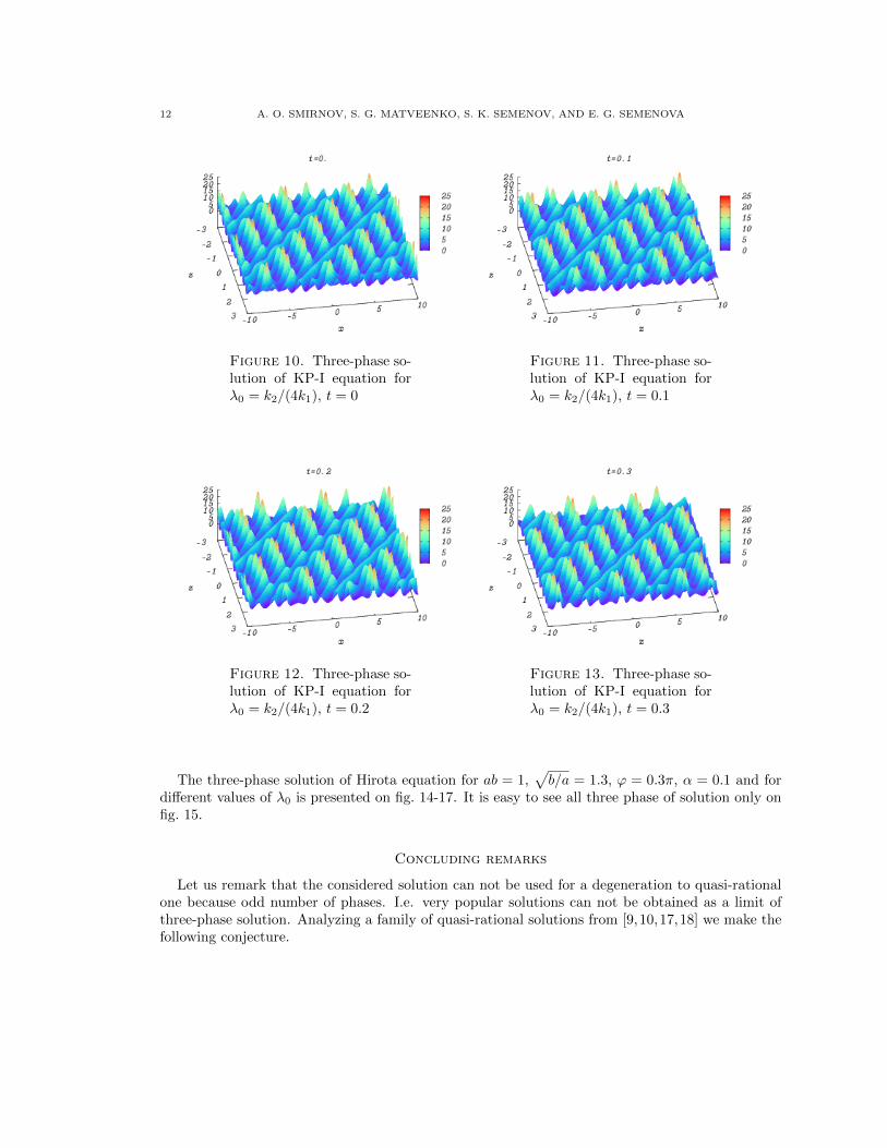
The three-phase solution of KP-I equation for ab = 1,√b/a = 1.3, ϕ = 0.3π at the different

moment of time t and for λ0 = 0 is presented on the fig. 6-9. The same solution for λ0 = k2/(4k1)one can see on the fig. 10-13. It is easy to see all three phase of solution on figures 6-13. Twophase are shortwave and third phase is a long-wave envelope. One can see also on fig. 6-9 that thesolution for λ0 = 0 is periodic in z, and that the long-wave envelope move to the right side.

Figure 6. Three-phase so-lution of KP-I equation forλ0 = 0, t = 0

Figure 7. Three-phase so-lution of KP-I equation forλ0 = 0, t = 0.1




Figure 10. Three-phase so-lution of KP-I equation forλ0 = k2/(4k1), t = 0

Figure 11. Three-phase so-lution of KP-I equation forλ0 = k2/(4k1), t = 0.1



The three-phase solution of Hirota equation for ab = 1,√b/a = 1.3, ϕ = 0.3π, α = 0.1 and for

different values of λ0 is presented on fig. 14-17. It is easy to see all three phase of solution only onfig. 15.

Concluding remarks

Let us remark that the considered solution can not be used for a degeneration to quasi-rationalone because odd number of phases. I.e. very popular solutions can not be obtained as a limit ofthree-phase solution. Analyzing a family of quasi-rational solutions from [9,10,17,18] we make thefollowing conjecture.


Figure 14. Amplitude ofthree-phase solution of Hi-rota equation for λ0 = 0

Figure 15. Amplitude ofthree-phase solution of Hi-rota equation for λ0 = 4

Figure 16. Amplitude ofthree-phase solution of Hi-rota equation for λ0 =k2/(4k1)

Figure 17. Amplitude ofthree-phase solution of Hi-rota equation for λ0 =k2/(4k3)

(1) Quasi-rational rang n solution of NLS equation can be obtained as a limit of 2n-phaseelliptic solution.

(2) Spectral curve of corresponding elliptic solution should be a 2-sheet unramified coveringover spectral curve of n-phase elliptic solution of KdV equation.

The rang 1 quasi-rational solution (Peregrine soliton) was obtained as limit of two-phase ellipticone in [44], and for obtaining rang 2 quasi-rational solution we should use a spectral curve of genusg = 4.

Authors acknowledge Prof. V.B. Matveev for his support and discussion over this paper andquasi-rational solutions of NLS equation. This work performed within the framework of the state


order of the Ministry of education of Russia, and partially supported by RFBR, research project14-01-00589 a.

References

[1] N. I. Akhiezer, Elements of the theory of elliptic functions, American Mathematical Society, Providence, RI,1990, Translated from the second Russian edition by H. H. McFaden.

[2] N. Akhmediev and E. Pelinovsky (eds.), Discussion & debate: Rogue waves - towards a unifying concept?, Eur.

Phys. J. Special Topics, vol. 185, Springer, 2010.[3] N. N. Akhmediev and A. Ankiewicz, Solitons, nonlinear pulses and beams, CHAPMAN & HALL, 1997.

[4] A. Ankiewicz, J. M. Soto-Crespo, and N. Akhmediev, Rogue waves and rational solutions of the Hirota equation,

Phys. Rev. E 81 (2010).[5] H. F. Baker, Abel’s theorem and the allied theory including the theory of theta functions, Cambridge, 1897.

[6] E. D. Belokolos, A. I. Bobenko, V. Z. Enol’skii, A. R. Its, and V. B. Matveev, Algebro-geometrical approach to

nonlinear evolution equations, Springer Ser. Nonlinear Dynamics, Springer, 1994.[7] R. Y. Chiao, E. Garmire, and C. H. Townes, Self-trapping of optical beams, Phys. Rev. Lett. 13 (1964), no. 15,

479–482.

[8] C. Q Dai and J. F. Zhang, New solitons for the Hirota equation and generalized higher-order nonlinearSchrodinger equation with variable coefficients, J. Phys. A 39 (2006), 723–737.

[9] P. Dubard and V. B. Matveev, Multi-rogue waves solutions: from the NLS equation to the KP-I equation,

Nonlinearity 26 (2013), no. 12, R93–R125.[10] Ph. Dubard, Multirogue solutions to the focusing nls equation, Ph.D. Thesis, 2010.

[11] B. A. Dubrovin, Inverse problem for periodic finite-zoned potentials in the theory of scattering, Funct. Anal.Appl. 9 (1975), no. 1, 61–62.

[12] , Periodic problems for the Korteweg-de Vries equation in the class of finite band potentials, Funct. Anal.

Appl. 9 (1975), no. 3, 215–223.[13] , Theta functions and non-linear equations, Russ. Math. Surv. 36 (1981), no. 2, 11–92.

[14] B. A. Dubrovin, V. B. Matveev, and S. P. Novikov, Nonlinear equations of Korteweg-de Vries type, finite-band

linear operators and Abelian varietes, Russ. Math. Surv. 31 (1976), no. 1, 59–146.[15] B. A. Dubrovin and S. P. Novikov, A periodicity problem for the Korteweg-de Vries and Sturm-Liouville equa-

tions. Their connection with algebraic geometry, Sov. Math., Dokl. 15 (1974), 1597–1601.[16] J. D. Fay, Theta-functions on Riemann surfaces, Lect. Notes in Math., vol. 352, Springer, 1973.

[17] P. Gaillard, Deformations of third-order Peregrine breather solutions of the nonlinear Schrodinger equation

with four parameters, Phys. Rev. E 88 (2013).[18] , Ten-parameter deformations of the sixth-order Peregrine breather solutions of the NLS equation, Phys-

ica Scripta 89 (2014).

[19] F. Gesztesy and H. Holden, Soliton equation and their algebro-geometric solutions: Vol. 1, (1+1)-dimensionalcontinuous models, Cambridge Stud. in Adv. Math., vol. 79, Cambridge University Press, 2003.

[20] F. Gesztesy, H. Holden, J. Michor, and G. Teschl, Soliton equation and their algebro-geometric solutions: Vol.

2, (1+1)-dimensional discrete models, Cambridge Stud. in Adv. Math., vol. 114, Cambridge University Press,2008.

[21] B. Guo, L. Ling, and Q. P. Liu, Nonlinear Schrodinger equation: Generalized Darboux transformation and rogue

wave solutions, Phys. Rev. E 85 (2012).[22] A. R. Its, “isomonodromy” solutions of equations of zero curvature, Mathematics of the USSR-Izvestiya 26

(1986), no. 3, 497–529.[23] A. R. Its and V. P. Kotlyarov, On a class of solutions of the nonlinear Schrodinger equation, Dokl. Akad. Nauk

Ukrain. SSR, Ser. A 11 (1976), 965–968, (Russian).

[24] A. R. Its and V. B. Matveev, Hill’s operator with finitely many gaps, Funct. Anal. Appl. 9 (1975), no. 1, 65–66.[25] , Schrodinger operators with finite-gap spectrum and n-soliton solutions of the KdV equation, Theor.

Math. Phys. 23 (1975), no. 1, 343–355.

[26] A.R. Its, Inversion of hyperelliptic integrals and integration of non-linear differential equations, Vestn. Leningr.Univ. (Mat. Mekh. Astron.) 7 (1976), no. 2, 39–46, (Russian).

[27] C. Kalla and C. Klein, New construction of algebro-geometric solutions to the Camassa-Holm equation andtheir numerical evaluation, Proc. R. Soc. A 468 (2012), no. 2141, 1371–1390.


[28] , On the numerical evaluation of algebro-geometric solutions to integrable equations, Nonlinearity 25(2012), no. 3, 569–596.

[29] A. Krazer, Lehrbuch der thetafunktionen, Teubner, Leipzig, 1903.

[30] I. M. Krichever, Methods of algebraic geometry in the theory of non-linear equations, Russ. Math. Surv. 32(1977), no. 6, 185–213.

[31] A. Kundu, A. Mukherjee, and T. Naskar, Modelling rogue waves through exact dynamical lump soliton controlledby ocean currents, Preprint, arXiv:1204.0916, 2012, 5p.

[32] E. A. Kuznetsov, Solitons in a parametricaly unstable plasma, Sov. Phys., Dokl. 22 (1977), 507–508.

[33] P. D. Lax, Periodic solutions of the K-dV equations, Lect. in Appl. Math. 15 (1974), 85–96.[34] Ch. Zh. Li and J. S. He, Darboux transformation and positons of the inhomogeneous Hirota and the Maxwell-

Bloch equation, Preprint, arXiv:1210.2501, 2012, 5p.

[35] V. A. Marchenko, The periodic Korteweg-de Vries problem, Math. USSR Sb. 24 (1974), no. 3, 319–344.[36] V. B. Matveev, 30 years of finite-gap integration theory, Phil. Trans. R. Soc. A 366 (2008), 837–875.

[37] H. P. McKean and P. van Moerbeke, The spectrum of Hill’s equation, Invent. Math. 30 (1975), 217–274.

[38] D. Mumford, Tata lectures on theta. II, Progress in Math., vol. 43, Birkhauser Boston Inc., Boston, MA, 1984.[39] S. P. Novikov, The periodic problem for the Korteweg-de Vries equation. i, Funct. Anal. Appl. 8 (1974), no. 3,

236–246.

[40] E. Previato, Hyperelliptic quasi-periodic and soliton solutions of the nonlinear Schrodinger equation, DukeMath. J. 52 (1985), no. 2, 281–545.

[41] A. O. Smirnov, A matrix analogue of the Appell theorem and reduction of multidimensional Riemann theta-

functions, Math. USSR Sb. 61 (1988), no. 2, 379–388.[42] , Elliptic solutions of the nonlinear Schrodinger equation and the modified Korteweg-de Vries equation,

Russ. Acad. Sci. Sb. Math. 82 (1995), no. 2, 461–470.[43] , Solution of a nonlinear Schrodinger equation in the form of two-phase freak waves, Theor. Math. Phys.

173 (2012), no. 1, 1403–1416.

[44] , The elliptic breather for the nonlinear Schrodinger equation, J. Math. Sci. 192 (2013), no. 1, 117–125.[45] , Periodic two-phase “rogue waves”, Math. Notes 94 (2013), no. 6, 897–907.

[46] A. O. Smirnov, E. G. Semenova, V. Zinger, and N. Zinger, On a periodic solution of the focusing nonlinear

Schrodinger equation, Preprint, arXiv:1407.7974, 2014, 24p.[47] L. H. Wang, K. Porsezian, and J. S. He, Breather and rogue wave solutions of a generalized nonlinear Schrodinger

equation, Preprint, arXiv:1304.8085, 2013, 21p.[48] Z. Yan, Financial rogue waves appearing in the coupled nonlinear volatility and option pricing model, Preprint,

arXiv:1101.3107, 2011.

[49] V. E. Zakharov, Stability of periodic waves of finite amplitude on the surface of a deep fluid, J. Appl. Mech.Tech. Phys. 9 (1968), no. 2, 190–194.

E-mail address: [email protected]




St.-Petersburg State University of Aerospace Instrumentation (SUAI), 67 Bolshaya Morskaya str.,

St.-Petersburg, 190000,Russia

http://arxiv.org/abs/1204.0916





mailto:[email protected]




three-phase freak waves - arxiv · three-phase freak waves a. o. smirnov, s. g. matveenko, s. k....

Documents