three-slit interference: a duality relation2. three-slit interference three slit interference is...
TRANSCRIPT

Prog. Theor. Exp. Phys. 2015, 083A02 (11 pages)DOI: 10.1093/ptep/ptv112
Three-Slit Interference: A Duality Relation
Mohd Asad Siddiqui and Tabish Qureshi
Centre for Theoretical Physics, Jamia Millia Islamia, New Delhi, India.∗E-mail: [email protected]
. . . . . . . . . . . . . . . . . . . . . . . . . . . . . . . . . . . . . . . . . . . . . . . . . . . . . . . . . . . . . . . . . . . . . . . . . . . . . . .
The issue of interference and which-way information is addressed in the context of3-slit interference experiments. A new path distinguishability DQ is introduced, basedon Unambiguous Quantum State Discrimination (UQSD). An inequality connecting the
interference visibility and path distinguishability, V +2DQ3−DQ ≤ 1, is derived which puts
a bound on how much fringe visibility and which-way information can be simultaneouslyobtained. It is argued that this bound is tight. For 2-slit interference, we derive a newduality relation which reduces to Englert’s duality relation and Greenberger-Yasin’sduality relation, in different limits.
1. Introduction
The two-slit interference experiment with particles has become a cornerstone for studying
wave-particle duality. So fundamental is the way in which the two-slit experiment captures
the essence of quantum theory, that Feynman ventured to state that it is a phenomenon
“which has in it the heart of quantum mechanics; in reality it contains the only mystery”
of the theory [1]. That radiation and massive particles can exhibit both wave nature and
particle nature in different experiment, had become quite clear in the early days of quantum
mechanics. However, Niels Bohr emphasized that wave-nature, characterized by two-slit
interference, and the particle-nature, characterized by the knowledge of which slit the particle
passed through, are mutually exclusive [2]. In doing this he raised this concept to the level
of a new fundamental principle.
Much later, this principle was made quantitatively precise by deriving a bound on the
extent to which the two natures could be observed simultaneously, by Greenberger and Yasin
[3] and later by Englert [4]. Greenberger and Yasin characterised the particle nature by the
ability to correctly predict which slit the particle passed through [3]. This predictability was
based only on the initial state of the particle, and not on any measurement on it. Englert
characterised the particle nature by the ability to distinguish between the two paths of the
particle, by an actual measurement [4]. He introduced a quantity D for this purpose, which
took values between 0 and 1. The wave nature was characterised by the visibility of the
interference, given by V. The relation putting a bound on the path distinguishability and
fringe visibility is given by [4]
V2 +D2 ≤ 1. (1)
Thus one can see that D and V, which can take values between 0 and 1, are dependent on
each other. A full which-way information (D = 1) would surely wash out the interference
(V = 0). Eqn. (1) can be thought to be a quantitative statement of Bohr’s complementarity
c© The Author(s) 2012. Published by Oxford University Press on behalf of the Physical Society of Japan.
This is an Open Access article distributed under the terms of the Creative Commons Attribution License
(http://creativecommons.org/licenses/by-nc/3.0), which permits unrestricted use,
distribution, and reproduction in any medium, provided the original work is properly cited.
arX
iv:1
405.
5721
v4 [
quan
t-ph
] 2
7 A
ug 2
015

Source
ScreenTripleSlit
11
2
3
D
1
2
3
2
1
D
1
2
3
da
db
Which-pathdetector
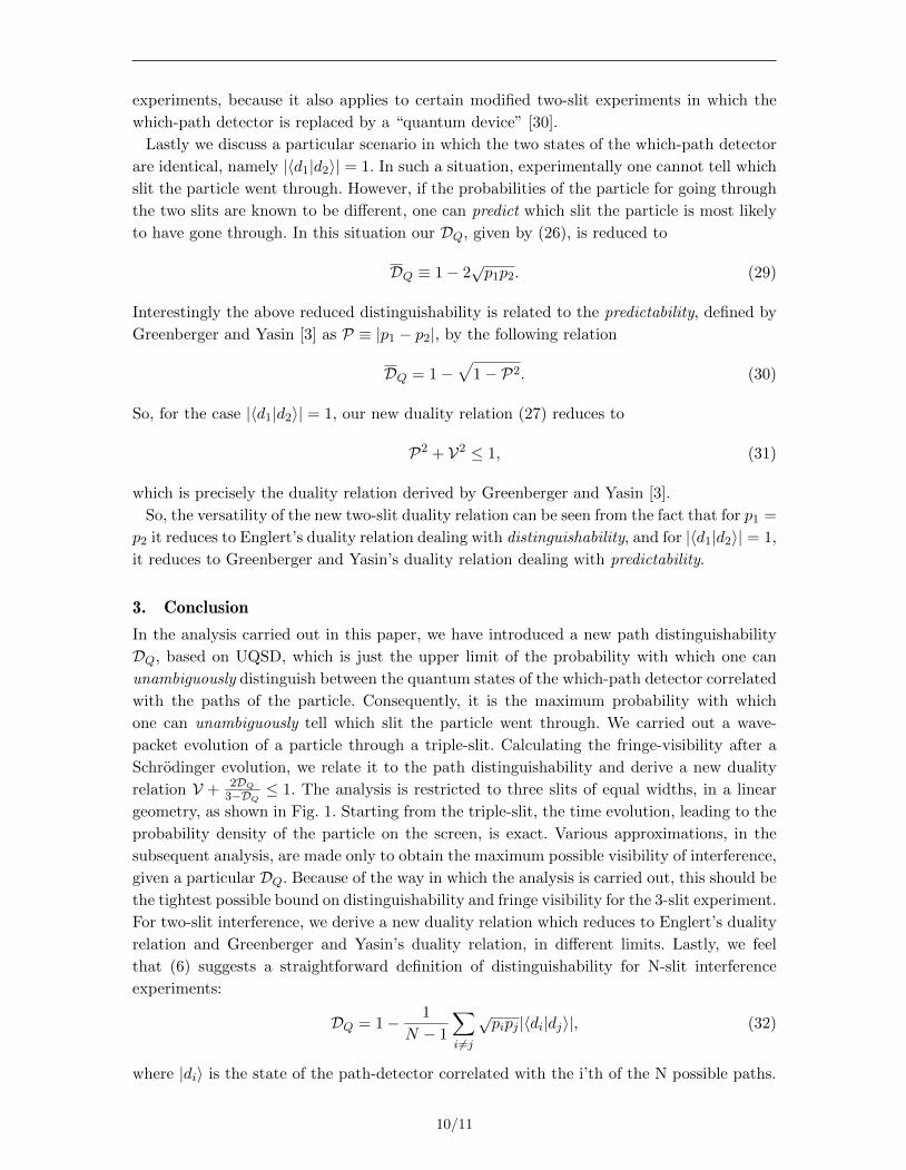
Fig. 1 A schematic diagram of the 3-slit interference experiment, with a quantum which-
path detector.
principle. It smoothly interpolates between the two extreme scenarios discussed by Bohr,
namely, full which-way information and no which-way information.
A dramatic manifestation of Bohr’s complementarity principle has been demonstrated
in the so-called quantum eraser. Here, “erasing” the which-way information after the par-
ticle has passed through the slits, allows one to recover the lost interference fringes [5].
Wave-particle duality has also been connected to various other phenomena. Connection
of wave-particle duality with uncertainty relations has been investigated [6–9]. An inter-
esting complementarity between entanglement and the visibility of interference has been
demonstrated for two-path interference [10]. That the entanglement between the particle
and which-path detector is what affects the visibility of interference, is also the view we take
in this investigation.
Various aspects of complementarity were also explored by Jaeger, Shimony and Vaidman
[11] where they also explored the case where the particle can follow multiple path, and
not just two, before interfering. Bohr’s principle of complementarity should surely apply to
multi-slit experiments too. However, one might wonder if one can find a quantitatively precise
statement of it for multi-slit experiments. Various attempts have been made to formulate
a quantitatively precise statement of complementarity, some kind of a duality relation, for
the case of multibeam interferometers [12–16]. However, the issue is still not satisfactorily
resolved. Beyond the well studied two-slit experiment, the simplest multi-beam case is the
3-slit interference experiment. Englert’s duality relation was derived only in the context of 2-
slit experiments, and one would like an analogous relation for the case of 3-slit experiments.
That is the focus of this paper. Of late there has been a newly generated focus on the
three-slit interference experiments [17–19], albeit for a different reason.
2/11

2. Three-slit interference
Three slit interference is somewhat more involved than its 2-slit counterpart simply due to
the fact that while the two-slit interference is the result of interference between two parts
coming from the two slits, in the 3-slit interference there are three parts which interfere in
different ways. In the general case, if we assume that the separation between slits 1 and 2 is
`1 and that between slits 2 and 3 is `2, there are two interferences from slit 1 and 2 and from
slit 2 and slit 3. In addition there is an interference between parts from slit 1 and 3, which
involves a slit separation of `1 + `2. In the case where the two slit separations are the same,
`1 = `2 = d, there are two interferences with slit separation d and one interference with slit
separation 2d. Having more than two slits also allows, in principle, the possibility of having
different geometrical arrangement of slits. However, we restrict ourselves to the case of three
slits in a linear geometry, as shown in Fig. 1, as that is the geometry in which the experiment
is usually done, and that is also the geometry which is used in previous investigations of
multi-slit experiments.
We expect additional complicacy in interpreting Bohr’s complementarity because if we
know that the particle did not go through (say) slit 3, it may not imply complete loss of
interference as there is still ambiguity regarding which of the other two slits, 1 or 2, the
particle went through.
2.1. Which-way information
First we would like to have a way of knowing which of the three slits the particle passed
through. Any which-path detector should have three states which should correlate with the
particle passing through each slit. Let these states be |d1〉, |d2〉, |d3〉, which correspond to
particle passing through slits 1, 2 and 3, respectively. Without loss of generality we assume
that the states |d1〉, |d2〉, |d3〉 are normalized, although they may not necessarily be mutually
orthogonal. The combined state of the particle and the which-path detector can be written
as
|Ψ〉 =√p1|ψ1〉|d1〉+
√p2|ψ2〉|d2〉+
√p3|ψ3〉|d3〉, (2)
where√p1|ψ1〉,
√p2|ψ2〉,
√p3|ψ3〉 are the amplitudes of the particle passing through the slit
1, 2 and 3, respectively. Particle passes through slits 1, 2, and 3 with probabilities p1, p2 and
p3, respectively.
If |d1〉, |d2〉, |d3〉 are mutually orthogonal, we can find a Hermitian operator (and thus, a
measurable quantity) which will give us different eigenvalues corresponding to |d1〉, |d2〉, |d3〉,and thus to the particle passing through each of the three slit. In this case, which slit the
particle went through, can be known without ambiguity.
If |d1〉, |d2〉, |d3〉 are not mutually orthogonal, the three ways of particle going through the
slits will not be fully distinguishable. One needs to define a distinguishability of the three
different paths of the particle. Defining distinguishability in multi-slit experiments has been
a thorny issue [11–15].
2.2. Unambiguous Quantum State Discrimination
As one can see from (2), the problem of distinguishing the three paths of the particle boils
down to distinguishing between the three states |d1〉, |d2〉, |d3〉. In the following we describe
a well established method of unambiguously discriminating between two non-orthogonal
3/11

quantum states, which goes by the name of Unambiguous Quantum State Discrimination
(UQSD) [20–24]. If two states |p〉, |q〉 are not orthogonal, it is impossible to distinguish
between the two with certainty. What UQSD does is to separate the measurement results
into two categories. First category is the one in which the discrimination fails. The second
one distinguishes between the two states without any error. Let the first system, whose states
are |p〉, |q〉 interact with a second system which is initially in a state |s0〉. The interaction
and time evolution leads to the following entangled states
U |p〉|s0〉 = α|p1〉|s1〉+ β|p2〉|s2〉
U |q〉|s0〉 = γ|q1〉|s1〉+ δ|q2〉|s2〉, (3)
where U is a unitary operator such that 〈s1|s2〉 = 0 and 〈p1|q1〉 = 0. If one measures an
observable of the second system which has two eigenstates |s1〉, |s2〉 with different eigenvalues,
the result |s1〉 lands us into a situation where the non-orthogonal states |p〉, |q〉 have been
replaced by orthogonal |p1〉, |q1〉. The orthogonal states |p1〉, |q1〉 can be distinguished with
hundred percent accuracy, thus distinguishing the original |p〉, |q〉 without error. However, the
other result for system 2, |s2〉, leads us to states |p2〉, |q2〉 which are not orthogonal, and the
discrimination of |p〉, |q〉 fails. So, either the process fails, or it distinguishes between |p〉, |q〉without error. The probability of successfully distinguishing between |p〉 and |q〉 depends on
the constants α, β, γ, δ. It can be easily shown that the maximum probability of successfully
distinguishing between |p〉 and |q〉 is given by [21]
P = 1− |〈p|q〉|. (4)
This is called the IDP (Ivanovic-Dieks-Peres) limit, and |p〉 and |q〉 cannot be distinguished
unambiguously with a probability larger than this, even in principle [20–22]. In other words,
UQSD is the best bet for discriminating between two non-orthogonal states. This fact has also
been experimentally demonstrated recently [25, 26]. Thus, the IDP limit sets a fundamental
bound on the distinguishability of two non-orthogonal states.
2.3. Distinguishability
The preceding analysis suggests a natural definition of path-distinguishability. In a two-slit
experiment, if the combined state of the particle and the which way detector can be written
as |Ψ〉 = |ψ1〉|d1〉+ |ψ2〉|d2〉, the two paths can be distinguished if the two states |d1〉, |d2〉 can
be distinguished. The probability of successfully telling which slit the particle went through
is just the probability with which |d1〉, |d2〉 can be unambiguously distinguished. We thus
define distinguishability of the two paths in a double-slit experiment as the upper limit of
the probability of unambiguously distinguishing between |d1〉 and |d2〉. Thus we define a new
path distinguishability for a two-slit experiment as
DQ ≡ 1− |〈d1|d2〉|. (5)
We denote it by DQ to distinguish it from the D used in (1).
In the 3-slit experiment, the entangled state (2) implies that, after the particle has passed
through the triple slit, the which-path detector could be in state |d1〉 or |d2〉 or |d3〉, with
probabilities p1, p2 and p3, respectively. The probability with which one can tell which
of the three slits the particle went through, is just the probability with which one can
4/11

distinguish between |d1〉, |d2〉, |d3〉. So, the problem of distinguishing between the three paths
boils down to distinguishing between three non-orthogonal states |d1〉, |d2〉, |d3〉, which occur
with different probabilities.
UQSD has also been generalized to the case of N non-orthogonal states. The probability
of unambiguously distinguishing between N non-orthogonal quantum states is bounded by
[27, 28]
PN ≤ 1− 1
N − 1
∑i 6=j
√pipj |〈di|dj〉|, (6)
where |di〉 are the N non-orthogonal states, and pi are their respective a-priori probabili-
ties. For three non-orthogonal states, the above reduces to
P3 ≤ 1− (√p1p2|〈d1|d2〉|+
√p2p3|〈d2|d3〉|+
√p1p3|〈d1|d3〉|). (7)
We define the path-distinguishability for the 3-slit experiment as the upper limit of the
probability with which one can distinguish between the three states |d1〉, |d2〉, |d3〉, which is
now given by
DQ ≡ 1− (√p1p2|〈d1|d2〉|+
√p2p3|〈d2|d3〉|+
√p1p3|〈d1|d3〉|), (8)
and whose value lies in the range 0 ≤ DQ ≤ 1. Eqn. (8) should be seen as a generalization
of the IDP limit to the case of three non-orthogonal states.
2.4. Interference and which-way information
In order to obtain a tight bound on the visibility of interference, given a particular amount
of which-way information, we do a wave-packet analysis in the following way. We consider
a particle traveling along the z-direction and passing through the triple-slit, with a slit
separations `1 and `2, and then interacting with a which-path detector through a unitary
evolution. The evolution of the state is given by the time-dependent Schrodinger equation,
i~∂t|Ψ(t)〉 = H|Ψ(t)〉, (9)
where H is the Hamiltonian of the system (the energy operator).
Our strategy is the following. The motion of the particle along the z-axis is redundant,
as it only translates the position of the particle from the triple-slit to the screen. What is
relevant is the motion and dispersion of the particle along the x-direction. Without going
into the details of the which-path detector, we assume that it is a device having 3 states
|d1〉, |d2〉, |d3〉, which get entangled with the three amplitudes of the particle passing through
slits 1, 2 and 3, respectively. This entanglement is a necessary condition for the which-path
detector to get any information about which slit the particle went through [7].
In the following we assume that the mass of the particle is m, and the three slits are
located at x = +`1, 0, − `2. The wavefunction emerging from a particular slit is assumed
to be a Gaussian wave-packet in the x-direction, of width ε, localized at x = `1, 0, or − `2.
A wavefunction of the form e−(x−`1)2
4ε2 should represent the particle emerging from a slit of
width ε, located at x = `1, in a reasonable approximation. As we shall see later, the choice of
the Gaussian form does not lead to any loss of generality because the width of the Gaussians
does not appear in the final results.
5/11

Using this strategy, the combined state of the particle and the which-path detector, when
the particle emerges from the triple-slit (time t = 0), will be of the form
Ψ(x, 0) = A
(√p1|d1〉e−
(x−`1)2
4ε2 +√p2|d2〉e−
x2
4ε2 +√p3|d3〉e−
(x+`2)2
4ε2
), (10)
where A = (2πε2)−1/4, and p1 + p2 + p3 = 1. It represents three Gaussian wave-packets
localised at the three slits, namely x = `1, x = 0 and x = −`2, entangled with the three
states of the which-path detector. The width of the three Gaussians is chosen to be the same
because the widths of the three slits is assumed to be the same. It is not difficult to see, from
the subsequent analysis, that even if we consider the three slit-widths to be different, e.g.,
ε1, ε2, ε3, they would all drop out from our final result. In general one should consider a
factor√p1e
iθ instead of√p1, and likewise for
√p2 and
√p3. We do not consider these phase
factors simply because they will be absorbed in certain phases introduced later, in section
2.4. We consider the probabilities of all the three paths to be different for generality, but
point out that unequal probabilities reduce the visibility of interference. Even in the two-slit
interference, unequal beams reduce the visibility of interference.
After a time t, the state of the particle and the detector evolves via (9), with H = p2x/2m,
to
Ψ(x, t) = A
(√p1|d1〉e−
(x−`1)2
4ε2+2i~t/m +√p2|d2〉e−
x2
4ε2+2i~t/m +√p3|d3〉e−
(x+`2)2
4ε2+2i~t/m
), (11)
where A = [√
2π(ε+ i~t/2mε)]−1/2. It represents the three wave-packets spreading and over-
lapping with each other. The smaller the width ε of the slits, the stronger is the overlap
between the three wave-packets.
The probability (density) of finding the particle at a position x on the screen is given by
|Ψ(x, t)|2 = |A|2(p1e− (x−`1)2
2σ2 + p2e− x2
2σ2 + p3e− (x+`2)2
2σ2
+√p1p2e
− 2x2+`21−2x`1
4σ2
[〈d1|d2〉e
ix`1~t/m−i~t`21/2m
4Ω2 + 〈d2|d1〉e−ix`1~t/m−i~t`21/2m
4Ω2
]+√p2p3e
− 2x2+`22+2x`2
4σ2
[〈d2|d3〉e
ix`2~t/m+i~t`22/2m4Ω2 + 〈d3|d2〉e−
ix`2~t/m+i~t`22/2m
4Ω2
]+√p1p3e
− x2+(`21+`22)/2+x(`2−`1)
2σ2
[〈d1|d3〉e
i[x(`1+`2)+(`22−`21)/2]~t/m4Ω2
+〈d3|d1〉e−i[x(`1+`2)+(`22−`21)/2]~t/m
4Ω2
]), (12)
where σ2 = ε2 + (~t/2mε)2 and Ω2 = ε4 + (~t/2m)2. We write the overlaps of various detec-
tor states as: 〈d1|d2〉 = |〈d1|d2〉|eiθ1 , 〈d2|d3〉 = |〈d3|d3〉|eiθ2 , 〈d1|d3〉 = |〈d1|d3〉|eiθ3 . The phases
θ1, θ2, θ3 being arbitrary, any additional phases coming from the amplitudes of the initial
6/11

state (10) would be absorbed in them. The probability density then reduces to
|Ψ(x, t)|2 = |A|2(e−
x2
2σ2
(p1e− `
21−2x`1
2σ2 + p2 + p3e− `
22+2x`2
2σ2
)+2√p1p2|〈d1|d2〉|e−
2x2+`21−2x`1
4σ2 cos
(x`1~t4mΩ2
− β1 + θ1
)+2√p2p3|〈d2|d3〉|e−
2x2+`22+2x`2
4σ2 cos
(x`2~t4mΩ2
+ β2 + θ2
)+ 2√p1p3|〈d1|d3〉|e−
2x2+`21+`22+2x(`2−`1)
4σ2 cos
(x(`1 + `2)~t
4mΩ2+ β3 + θ3
)),(13)
where β1 = ~t`218mΩ2 , β2 = ~t`22
8mΩ2 , and β3 = ~t(`22−`21)8mΩ2 .
Visibility of the interference fringes is conventionally defined as [29]
V =Imax − IminImax + Imin
, (14)
where Imax and Imin represent the maximum and minimum intensity in neighbouring fringes,
respectively. Since all the factors multiplying the cosine terms in (13) are non-negative, the
maxima of the fringe pattern will occur where the value of all the cosines is +1. The minima
will occur where value of all the cosines is −1/2 at the same time.
2.5. Equally spaced slits
In the usual three-slit interference experiments, the three slits are equally spaced. In that
case `1 = `2 ≡ d, and β1 = β2 ≡ β and β3 = 0. Provided we ignore β, the cosines can indeed
have values all +1 or all −1/2 for certain values of x. Ignoring β amounts to ignoring d/2
in comparison to x, which is justified if one looks at any fringe except the central one (at
x = 0), since fringe width on the screen is much larger than the slit separation d. The ideal
visibility can then be written down as
VI =3(√
p1p2|〈d1|d2〉|exd
2σ2 +√p1p3|〈d1|d3〉|e−
d2
2σ2 +√p2p3|〈d2|d3〉|e−
xd
2σ2
)α+√p1p2|〈d1|d2〉|e
xd
2σ2 +√p1p3|〈d1|d3〉|e−
d2
2σ2 +√p2p3|〈d2|d3〉|e−
xd
2σ2
. (15)
where α = 2(p2 + [p1e
xd
σ2 + p3e−xdσ2 ]e−
d2
2σ2
). In reality, fringe visibility will be reduced due
many factors, including the width of the slits. For example, if the width of the slits is very
large, the fringes may not be visible at all. It will also get reduced by the varying phases
θ1, θ2, θ3. In an ideal situation, the maximum visibility one can theoretically get will be in the
case when d σ, which amounts to assuming that the spread of a particular wave-packet,
when it reaches the screen, is so large that the separation between two neighboring slits d is
negligible in comparison, and also when all the phases are either zero or their effect cancels
out. Actual fringe visibility will be less than or equal to that, and can be written as
V ≤3(√p1p2|〈d1|d2〉|+
√p1p3|〈d1|d3〉|+
√p2p3|〈d2|d3〉|
)2 +√p1p2|〈d1|d2〉|+
√p1p3|〈d1|d3〉|+
√p2p3|〈d2|d3〉|
. (16)
Using (8) the above equation gives
V +2DQ
3−DQ≤ 1. (17)
7/11

Eqn. (17) is a new duality relation which puts a bound on how much which-way information
we can obtain and how much fringe visibility we can get at the same time. It is straightfor-
ward to check that V = 1 is possible only for DQ = 0, and DQ = 1 implies V = 0. Note that
(17) can also be expressed in another form
DQ +2V
3− V≤ 1. (18)
2.6. Unequally spaced slits
When the three slits are equally spaced, maximum is achieved when the two cos(xd~t4mΩ2
)terms and the cos
(2xd~t4mΩ2
)term have values +1 at the same time, which happens when
xd~t4mΩ2 = 2nπ, provided that θ1, θ2, θ3 are zero. When the three slits are unequal, the three
terms cos(x`1~t4mΩ2
), cos
(x`2~t4mΩ2
)and cos
(x(`1+`2)~t
4mΩ2
)cannot all have values +1 at the same
time. Thus the maximum intensity will be smaller than that in the equally spaced case, or
Iunequalmax < Iequalmax .
Minimum intensity in the equally spaced case is attained when all the cosine terms are
equal to −1/2, which happens when xd~t4mΩ2 = 2nπ
3 , provided that θ1, θ2, θ3 are zero. When the
three slits are unequally spaced, the three terms cos(x`1~t4mΩ2
), cos
(x`2~t4mΩ2
)and cos
(x(`1+`2)~t
4mΩ2
)cannot all have values −1/2 at the same time. Thus the minimum intensity will be larger
than that in the equally spaced case, or Iunequalmin > Iequalmin . These two observations lead to the
straightforward conclusion that fringe visibility in the case of unequal slits will be strictly
smaller than that in the case of equal slits, other things being the same,
Vunequal < Vequal. (19)
Using the above in conjunction with (16) we can write for the fringe visibility, for the case
of unequal slits
V <3(√p1p2|〈d1|d2〉|+
√p1p3|〈d1|d3〉|+
√p2p3|〈d2|d3〉|
)2 +√p1p2|〈d1|d2〉|+
√p1p3|〈d1|d3〉|+
√p2p3|〈d2|d3〉|
. (20)
Using (8) the above equation gives
V +2DQ
3−DQ< 1. (21)
Note the strictly less than sign in the above, in contrast with (17). The above relation implies
that if the slits are unequally spaced, even if the distinguishability DQ is reduced to zero,
the visibility of interference can never be 1. The reason of this behaviour lies in the fact that
a certain amount of loss of interference visibility is rooted not in the path distinguishability,
but in the unequal spacing of the three slits.
2.7. Specific cases
Let us look at some special cases arising from the fact that there are not two, but three slit.
Suppose we have a which-path detector which can detect with certainty if the particle has
passed through slit 1 or not. If the particle has not passed through slit 1, the detector is
unable to say which of the other two slits, 2 or 3, has the particle taken. Such a scenario can
occur, for example, if we have a tiny camera in front of slit 1 which, for each particle, can say
if the particle has gone through slit 1 or not. In this case |d1〉 is orthogonal to both |d2〉 and
8/11

|d3〉, and |d2〉, |d3〉 are parallel. Thus, in this case, |〈d2|d3〉| = 1 and |〈d1|d2〉| = |〈d1|d3〉| = 0.
Assuming, for simplicity, p1 = p2 = p3 = 13 , the distinguishability DQ, in this case is
DQ ≡ 1− 1
3(|〈d1|d2〉|+ |〈d2|d3〉|+ |〈d1|d3〉|) =
2
3, (22)
Consequently, the fringe visibility is limited by
V ≤ 3
7. (23)
Physically what is happening is the following. Particle going through slits 2 and 3 gives
rise to a sharp interference pattern, however, particle going through slit 1 gives rise to a
uniform background particle count, thus reducing the overall visibility of the fringes arising
from slits 2 and 3.
Let us consider another case where |d1〉 and |d2〉 are orthogonal to each other, but both
have equal overlap with |d3〉. Such a case can be exemplified by |d1〉 = 1√2(| ↑〉+ | ↓〉), |d2〉 =
1√2(| ↑〉 − | ↓〉) and |d3〉 = | ↑〉, where | ↑〉, | ↓〉 form an orthonormal set. In this case (again,
for simplicity, assuming p1 = p2 = p3 = 13) the distinguishability is
DQ = 1− 1
3(|〈d1|d2〉|+ |〈d2|d3〉|+ |〈d1|d3〉|) = 1−
√2
3, (24)
Consequently, the fringe visibility is limited by
V ≤ 3√
2
6 +√
2. (25)
2.8. The two-slit experiment
Just for completeness, here we wish to derive a duality relation for a two-slit experiment
in the case where one defines path distinguishability based on UQSD. We define the distin-
guishability of two paths as the upper limit of (6) for N=2. The path distinguishability then
reads
DQ ≡ 1− 2√p1p2|〈d1|d2〉|, (26)
where p1 and p2 are the probabilities of the particle to go through the first and the second
slit, respectively.
By carrying out an analysis similar to the one earlier in this section (essentially, putting
p3 = 0 in (13) and redefining some constants), one can show that the distinguishability and
fringe visibility, in the two-slit experiment, are bounded by
V +DQ ≤ 1. (27)
The above relation is a simple wave-particle duality relation for a two-slit interference
experiment where the beams may be unequal.
It can be connected to Englert’s duality relation (1) for the case p1 = p2 = 1/2. In Englert’s
analysis, distinguishability is given by D ≡√
1− |〈d1|d2〉|2 [4], which can be related to DQin (26), for p1 = p2 = 1/2, by the relation
DQ = 1−√
1−D2. (28)
If one plugs in the above form of DQ in (27), the latter reduces to V2 +D2 ≤ 1, which is just
Englert’s duality relation (1). The new relation (27) appears to be more versatile for two-slit
9/11
experiments, because it also applies to certain modified two-slit experiments in which the
which-path detector is replaced by a “quantum device” [30].
Lastly we discuss a particular scenario in which the two states of the which-path detector
are identical, namely |〈d1|d2〉| = 1. In such a situation, experimentally one cannot tell which
slit the particle went through. However, if the probabilities of the particle for going through
the two slits are known to be different, one can predict which slit the particle is most likely
to have gone through. In this situation our DQ, given by (26), is reduced to
DQ ≡ 1− 2√p1p2. (29)
Interestingly the above reduced distinguishability is related to the predictability, defined by
Greenberger and Yasin [3] as P ≡ |p1 − p2|, by the following relation
DQ = 1−√
1− P2. (30)
So, for the case |〈d1|d2〉| = 1, our new duality relation (27) reduces to
P2 + V2 ≤ 1, (31)
which is precisely the duality relation derived by Greenberger and Yasin [3].
So, the versatility of the new two-slit duality relation can be seen from the fact that for p1 =
p2 it reduces to Englert’s duality relation dealing with distinguishability, and for |〈d1|d2〉| = 1,
it reduces to Greenberger and Yasin’s duality relation dealing with predictability.
3. Conclusion
In the analysis carried out in this paper, we have introduced a new path distinguishability
DQ, based on UQSD, which is just the upper limit of the probability with which one can
unambiguously distinguish between the quantum states of the which-path detector correlated
with the paths of the particle. Consequently, it is the maximum probability with which
one can unambiguously tell which slit the particle went through. We carried out a wave-
packet evolution of a particle through a triple-slit. Calculating the fringe-visibility after a
Schrodinger evolution, we relate it to the path distinguishability and derive a new duality
relation V + 2DQ3−DQ ≤ 1. The analysis is restricted to three slits of equal widths, in a linear
geometry, as shown in Fig. 1. Starting from the triple-slit, the time evolution, leading to the
probability density of the particle on the screen, is exact. Various approximations, in the
subsequent analysis, are made only to obtain the maximum possible visibility of interference,
given a particular DQ. Because of the way in which the analysis is carried out, this should be
the tightest possible bound on distinguishability and fringe visibility for the 3-slit experiment.
For two-slit interference, we derive a new duality relation which reduces to Englert’s duality
relation and Greenberger and Yasin’s duality relation, in different limits. Lastly, we feel
that (6) suggests a straightforward definition of distinguishability for N-slit interference
experiments:
DQ = 1− 1
N − 1
∑i 6=j
√pipj |〈di|dj〉|, (32)
where |di〉 is the state of the path-detector correlated with the i’th of the N possible paths.
10/11

Acknowledgement
Mohd Asad Siddiqui thanks the University Grants Commission, India for financial support.
References
[1] R.P. Feynman, R.B. Leighton, M. Sands, The Feynman Lectures on Physics (Addison-Wesley 1966) Vol.3, pp. 1-1.
[2] N. Bohr, “The quantum postulate and the recent development of atomic theory,” Nature (London) 121,580-591 (1928).
[3] D.M. Greenberger, A. Yasin, “Simultaneous wave and particle knowledge in a neutron interferometer”,Phys. Lett. A 128, 391 (1988).
[4] B-G. Englert, “Fringe visibility and which-way information: an inequality”, Phys. Rev. Lett. 77, 2154(1996).
[5] S.P. Walborn, M.O. Terra Cunha, S.Padua, C.H. Monken, “Quantum erasure”, American Scientist 91,336-343 (2003).
[6] S. Durr, G. Rempe, “Can wave-particle duality be based on the uncertainty relation?,” Am. J. Phys. 68,1021-1024 (2000).
[7] T. Qureshi, R. Vathsan, “Einstein’s recoiling slit experiment, complementarity and uncertainty”, Quanta2, 58-65 (2013). DOI: 10.12743/quanta.v2i1.11
[8] P.J. Coles, J. Kaniewski, S. Wehner, “Equivalence of wave-particle duality to entropic uncertainty,”Nature Communications 5, 5814 (2014).
[9] S. Tanimura, “Complementarity and the nature of uncertainty relations in Einstein-Bohr recoiling slitexperiment,” Quanta 4, 1-9 (2015). DOI: 10.12743/quanta.v4i1.35
[10] A. Hosoya, A. Carlini, S. Okano, “Complementarity of entanglement and interference,” Int. J. Mod.Phys. C 17, 493 (2006). DOI: 10.1142/S0129183106008716
[11] G. Jaeger, A. Shimony, L. Vaidman, “Two interferometric complemenarities,” Phys. Rev. A 51, 54(1995).
[12] S. Durr, “Quantitative wave-particle duality in multibeam interferometers,” Phys. Rev. A 64, 042113(2001).
[13] G. Bimonte, R. Musto, “Comment on ‘Quantitative wave-particle duality in multibeam interferome-ters’,” Phys. Rev. A 67, 066101 (2003).
[14] G. Bimonte, R. Musto, “On interferometric duality in multibeam experiments” J. Phys. A: Math. Gen.36, 11481 (2003). (2003).
[15] B-G. Englert, “Wave-particle duality in multi-path interferometers: General concepts and three-pathinterferometers,” Int. J. Quantum Inform. 6, 129 (2008).
[16] M. Zawisky, M. Baron, R. Loidl, “Three-beam interference and which-way information in neutroninterferometry,” Phys. Rev. A 66, 063608 (2002).
[17] U. Sinha, C. Couteau, T. Jennewein, R. Laflamme, G. Weihs, “Ruling Out Multi-Order Interference inQuantum Mechanics”, Science 329, 418-421 (2010).
[18] H.D. Raedt, K. Michielsen, K. Hess, “Analysis of multipath interference in three-slit experiments”, Phys.Rev. A 85, 012101 (2012).
[19] R. Sawant, J. Samuel, A. Sinha, S. Sinha, U. Sinha, “Nonclassical paths in quantum interferenceexperiments,” Phys. Rev. Lett. 113, 120406 (2014).
[20] I.D. Ivanovic, “How to differentiate between non-orthogonal states”, Phys. Lett. A 123, 257 (1987).[21] D. Dieks, “Overlap and distinguishability of quantum states,” Phys. Lett. A 126, 303 (1988).[22] A. Peres, “How to differentiate between non-orthogonal states ,” Phys. Lett. A 128, 19 (1988).[23] G. Jaeger, A. Shimony, “Optimal distinction between two non-orthogonal quantum states,” Phys. Lett.
A 197, 83 (1995).[24] J.A. Bergou, U. Herzog, M. Hillery, “Discrimination of quantum states,” Lect. Notes Phys. 649, 417-465
(2004).[25] G. Waldherr, A.C. Dada, P. Neumann, F. Jelezko, E. Andersson, J. Wrachtrup, “Distinguishing between
nonorthogonal quantum states of a single nuclear spin,” Phys. Rev. Lett. 109, 180501 (2012).[26] M. Agnew, E. Bolduc, K.J. Resch, S. Franke-Arnold, J. Leach, “Discriminating single-photon states
unambiguously in high dimensions,” Phys. Rev. Lett. 113, 020501 (2014).[27] S. Zhang Y. Feng, X. Sun, M. Ying, “Upper bound for the success probability of unambiguous
discrimination among quantum states,” Phys. Rev. A 64, 062103 (2001).[28] D. Qiu, “Upper bound on the success probability for unambiguous discrimination,” Phys. Lett. A 303,
140-146 (2002)[29] M. Born, E. Wolf, “Principles of Optics” (Cambridge University Press, UK, 2002), 7th edition.[30] T. Qureshi, “Quantum twist to complementarity: A duality relation”, Prog. Theor. Exp. Phys. 2013,
11/11

041A01 (2013).
12/11