Three Sources of Increasing Returns to Scale

Jinill Kim�

First draft: March 1996This draft: April 3, 1997

Abstract

This paper reviews various types of increasing returns from a critical per-

spective. Increasing returns have been introduced both at the �rm level and

at the aggregate level in a monopolistic-competition model. We show that

the degree of the aggregate returns to scale is a linear combination of three

return parameters, with the weights determined by the speci�cation of a zero-

pro�t condition. Identi�cation issues are discussed with an emphasis on recent

macro literature. We argue that disaggregate data give information on the

market structure rather than the technology. Welfare implications explain

why it is important to identify various increasing returns.

Key words: Increasing Returns; Monopolistic Competition; Returns to Vari-

ety

JEL classi�cation: E32

�Federal Reserve Board, Mail Stop 61, Washington, D.C. 20551. Telephone: (202) 452-2715.

E-mail: jkim@frb.gov. This is a revised version of a chapter in my dissertation at Yale University.

Special thanks to Christopher Sims for his guidance and support. Thanks also to William Brainard,

John Fernald, Robert Shiller, Steve Sumner, Michael Woodford, and seminar participants at the

Universities of Maryland and Virginia, and Federal Reserve Board for their valuable comments.

This paper represents the view of the author and should not be interpreted as re ecting the views

of the Board of Governors of the Federal Reserve System or other members of its sta�.

1

Contents

1 Introduction 2

2 The Model 4

2.1 Firms . . . . . . . . . . . . . . . . . . . . . . . . . . . . . . . . . . . 5

2.2 Aggregation . . . . . . . . . . . . . . . . . . . . . . . . . . . . . . . . 8

2.3 Returns to Scale . . . . . . . . . . . . . . . . . . . . . . . . . . . . . 10

2.4 A Dynamic Model . . . . . . . . . . . . . . . . . . . . . . . . . . . . 15

3 Implications 19

3.1 Identi�cation with Aggregate Data . . . . . . . . . . . . . . . . . . . 19

3.2 Interpretation of Disaggregate Data . . . . . . . . . . . . . . . . . . . 21

3.3 Comparison with a Social Planner . . . . . . . . . . . . . . . . . . . . 24

4 Further research 26

A External Increasing Returns 28

B Input Fixed Cost 29

C Cost Minimization 31

D Fixed Cost Externalities 33

1 Introduction

The hypothesis of noncompetitive markets and/or increasing returns to scale has

recently been used in dynamic stochastic general-equilibrium (DSGE), more often

called real-business-cycle, models. Using the Solow residual as a measure of produc-

tivity changes is appropriate only under the joint hypothesis of perfectly competitive

markets and constant returns to scale. In a series of papers, Hall (1986, 1988, 1990)

argues that evidence from the Solow residual is not consistent with this maintained

hypothesis but with the alternative hypothesis of noncompetitive markets and/or in-

creasing returns to scale.1 Under this alternative hypothesis, the Solow residual has

1Imperfect competition makes equilibrium possible in the presence of increasing returns. In-

creasing returns are compatible with competitive �rms if the increasing returns are external to the

�rms. Internal returns may be motivated as a representation of external ones, as in Beaudry and

Devereux (1995a). The two types are compared using models with both types of increasing returns

in Appendix A.

2

endogenous components which cause it to over-represent the contribution of produc-

tivity shocks. Furthermore, this alternative hypothesis helps explain some puzzles

in the DSGE literature, e.g. little correlation between employment and productivity.

Following Dixit and Stiglitz (1977) and Blanchard and Kiyotaki (1987), the

monopolistic-competition framework has been widely used in macroeconomics. The

assumption of unrestricted entry and exit implies that pro�ts are zero in equilib-

rium.2 In a monopolistically competitive market, the technology of constant returns

to scale lets �rms produce positive pro�ts regardless of their size. Introducing in-

creasing returns at the �rm level leaves room for reducing pro�ts to zero.3 The

objective of this paper is to discuss three di�erent types of increasing returns in a

monopolistic-competitionmodel and to derive implications for the related literature.

There are two ways of introducing increasing returns at the �rm level. The

more conventional way is including �xed costs as part of a �rm's technology. This

way has been followed whenever a zero-pro�t condition is imposed. An alternate

way is amplifying the constant-returns-to-scale term by a power larger than one,

which amounts to diminishing marginal cost. When we incorporate both sources

of increasing returns simultaneously, as in Hornstein (1993), their e�ect on the ag-

gregate returns to scale is di�erent from each other. Increasing returns due to the

third source occurs only at the aggregate level. It involves a technology or a pref-

erence for the variety of goods. The introduction of a new good might enhance the

production e�ciency and the consumption convenience. Romer (1987) focuses on

this as an engine of growth and Matsuyama (1995) relates this to complementarities

and cumulative processes of macroeconomics. The model in Devereux, Head and

Lapham (1996a), even without productivity shocks, generates business cycle uc-

tuations of real variables from government spending shocks since these a�ect the

variety of goods.

This paper shows that, in a static model, the resulting degree of aggregate re-

turns to scale is the average of the second and the third sources of increasing returns,

without any in uence of positive �xed costs. The derivation of aggregate returns

from a �rm's technology involves two steps. First, the di�erentiated outputs are

aggregated to produce a measure of aggregate output. Second, a zero-pro�t con-

2See Benassy (1991) for quali�cations of zero-pro�t conditions. The assumption of zero pro�ts

matches the observation in Hall (1990) and Rotemberg and Woodford (1995) that there are no

signi�cant pure pro�ts in the United States.3Not that all papers in DSGE literature impose a zero-pro�t condition. Hairault and

Portier (1993) and Beaudry and Devereux (1995b) do not impose a zero-pro�t condition and

so parameterize both �xed cost and the number of �rms. In such models, the �rm-level returns

to scale are the aggregate returns to scale and the permanent presence of positive pro�ts remain

unexplained. For example, the steady-state pro�t rate is 17% in the benchmark model of Hairault

and Portier (1993).

3

dition is imposed upon the aggregate version of a �rm's technology. Speci�cation

of a zero-pro�t condition determines the weights of the averaging. In a dynamic

model where adjustments to zero pro�t are not instantaneous, the market structure

of monopolistic competition plays a role|the slower the adjustments, the larger the

role. Even if market structure does not directly a�ect the technology, this source

in uences the response of output in a way indistinguishable from the previous two

ways.

The aggregate dynamics of a model which combines various sources of increasing

returns to scale show that there are identi�cation problems in the recent macroe-

conomics literature using the framework of monopolistic competition. We compare

various papers to see how they specify a zero-pro�t condition and what the resulting

degree of returns to scale is. We also argue that the literature using disaggregate

data provides information di�erent from what it intends to provide: on the mar-

ket structure rather the technology. Lastly, welfare implications are discussed from

the perspective of a social planner who does not need to satisfy zero-pro�t condi-

tions. While having similar positive implications for the aggregate returns, various

increasing returns have di�erent normative implications.

2 The Model

To illustrate the points in as simple a structure as possible, we analyze only the

production side of the economy. This analysis is tractable and gives much insight

on how di�erent returns to scale interact with one another. Most papers on monop-

olistic competition deal with both the production and the consumption side of an

economy. However, introducing a utility function complicates the model so that it is

di�cult to disentangle the production features from consumer behavior. Our model

is a partial-equilibrium model, since the production side generates the demand for

inputs. The transformation of this model into a general-equilibrium framework is

straightforward by stacking it with a consumer problem and, if needed, a government

problem. The consumer problem would generate the supply function of aggregate

inputs through a labor-leisure choice and capital accumulation. Therefore, through-

out this paper, we may consider the aggregate inputs as exogenous variables.

Since a zero-pro�t condition is crucial in deriving the economy-wide returns to

scale, we will be very careful in discriminating two meanings of `production func-

tion.' A structural production function is a purely technological relation without

reference to the equilibrium condition of zero pro�ts. However, a production func-

tion in a reduced form, whether a �rm's or an aggregate one, is a combination of

the appropriate technology and a zero-pro�t condition. That is, a reduced-form

4

production function is a structural production function with a zero-pro�t condition

imposed.

Now our objective of this section is to transform a �rm-level structural pro-

duction function, Eq. (1), into an aggregate reduced-form production function, e.g.

Eqs. (16) and (24). This transformation is a contribution to the literature since it

simpli�es one step of complex DSGE models and so makes it easy to understand

their production features. We start with a static model since it is a special case

of a dynamic model. The static model serves as a steady-state, or low-frequency

in general, feature of the dynamic model. As a preparation for the analysis of the

aggregate variables, we analyze the behavior of �rms.

2.1 Firms

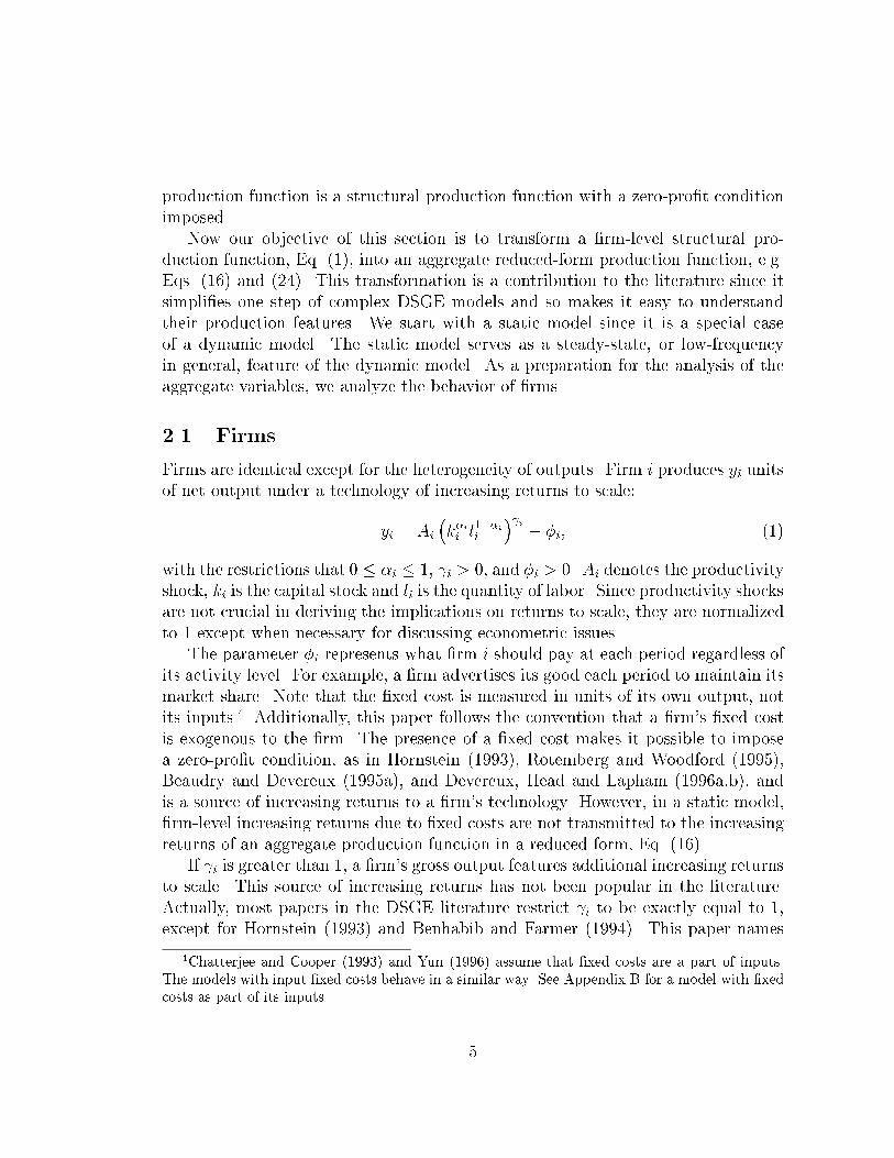
Firms are identical except for the heterogeneity of outputs. Firm i produces yi units

of net output under a technology of increasing returns to scale:

yi = Ai

�k�ii l1��ii

� i� �i; (1)

with the restrictions that 0 � �i � 1, i > 0, and �i > 0. Ai denotes the productivity

shock, ki is the capital stock and li is the quantity of labor. Since productivity shocks

are not crucial in deriving the implications on returns to scale, they are normalized

to 1 except when necessary for discussing econometric issues.

The parameter �i represents what �rm i should pay at each period regardless of

its activity level. For example, a �rm advertises its good each period to maintain its

market share. Note that the �xed cost is measured in units of its own output, not

its inputs.4 Additionally, this paper follows the convention that a �rm's �xed cost

is exogenous to the �rm. The presence of a �xed cost makes it possible to impose

a zero-pro�t condition, as in Hornstein (1993), Rotemberg and Woodford (1995),

Beaudry and Devereux (1995a), and Devereux, Head and Lapham (1996a,b), and

is a source of increasing returns to a �rm's technology. However, in a static model,

�rm-level increasing returns due to �xed costs are not transmitted to the increasing

returns of an aggregate production function in a reduced form, Eq. (16).

If i is greater than 1, a �rm's gross output features additional increasing returns

to scale. This source of increasing returns has not been popular in the literature.

Actually, most papers in the DSGE literature restrict i to be exactly equal to 1,

except for Hornstein (1993) and Benhabib and Farmer (1994). This paper names

4Chatterjee and Cooper (1993) and Yun (1996) assume that �xed costs are a part of inputs.

The models with input �xed costs behave in a similar way. See Appendix B for a model with �xed

costs as part of its inputs.

5

this source `diminishing marginal cost.' Appendix C on cost minimization shows

that the bigger i is, the smaller the slope of marginal cost is. Hornstein (1993)

call this `the scale coe�cient.' However, we will show that the degree of returns

to scale depends also on other parameters. Furthermore, diminishing marginal cost

may not a�ect the response of aggregate output, depending on the speci�cation of

a zero-pro�t condition.

These two sources of increasing returns to scale at the �rm level are added up

in overall returns to scale of a �rm's technology. From the perspective of a �rm,

to whom the �xed cost is exogenous, the log-linearized reduced-form production

function is:

yi '�k�ii l1��ii

�h i yi+�iyi

i:

That is, the degree of returns perceived by a �rm is the product of the degree of

diminishing marginal cost and the ratio between the gross and the net output. The

ratio turns out to be��

i

�, where � is the degree of market power. This degree

is assumed to be greater than i and de�ned in Eqs. (5) and (6). So the degree

of returns to scale of a �rm's technology is equal to the degree of market power.

However, this exercise is meaningless in that we have not incorporated a zero-pro�t

condition into a �rm's technology. Actually, we will see that the presence of �xed

costs by itself does not imply increasing returns in a static model. However, the

degree of market power turns out be the right measure in a dynamic case where

there are only steady-state adjustments to zero pro�t, without any period-by-period

adjustments.

A �rm maximizes its pro�t:5

�i = piyi � PZki � PWli;

where pi is the price of �rm i's product, P is the general price level, Z is the

real rental rate of capital, and W is the real wage. In models with monopolistic

competition, the price of outputs, pi, depends on the amount produced, yi. The

inverse demand for the output of the ith �rm will be derived later in Eq. (8),

which involves the parameter representing the market structure of monopolistic

competition, �. The assumption that �rms rent capital rather than holding and

accumulating it simpli�es the analysis. Under this assumption, we do not need

to explain where entering �rms buy capital or where exiting �rms sell remaining

5An alternative, and probably more conventional way of analyzing the �rm behavior is the

framework of cost minimization in Appendix C. However, the pro�t-maximization framework is

better for understanding the mechanics of the zero-pro�t condition since it expresses the endoge-

nous variables as a function of aggregate inputs, considered exogenous in this paper. Furthermore,

extension to a dynamic model becomes more complicated in the framework of cost minimization.

6

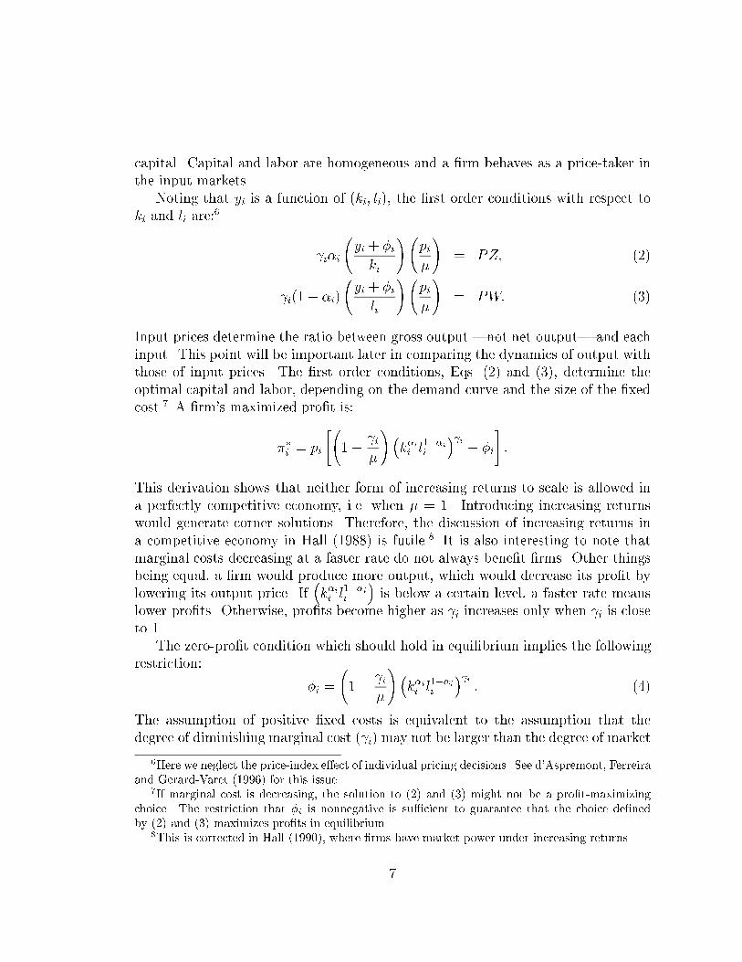
capital. Capital and labor are homogeneous and a �rm behaves as a price-taker in

the input markets.

Noting that yi is a function of (ki; li), the �rst order conditions with respect to

ki and li are:6

i�i

yi + �i

ki

! pi

�

!= PZ; (2)

i(1� �i)

yi + �i

li

! pi

�

!= PW: (3)

Input prices determine the ratio between gross output |not net output| and each

input. This point will be important later in comparing the dynamics of output with

those of input prices. The �rst order conditions, Eqs. (2) and (3), determine the

optimal capital and labor, depending on the demand curve and the size of the �xed

cost.7 A �rm's maximized pro�t is:

��i = pi

" 1�

i

�

!�k�ii l1��ii

� i� �i

#:

This derivation shows that neither form of increasing returns to scale is allowed in

a perfectly competitive economy, i.e. when � = 1. Introducing increasing returns

would generate corner solutions. Therefore, the discussion of increasing returns in

a competitive economy in Hall (1988) is futile.8 It is also interesting to note that

marginal costs decreasing at a faster rate do not always bene�t �rms. Other things

being equal, a �rm would produce more output, which would decrease its pro�t by

lowering its output price. If�k�ii l1��ii

�is below a certain level, a faster rate means

lower pro�ts. Otherwise, pro�ts become higher as i increases only when i is close

to 1.

The zero-pro�t condition which should hold in equilibrium implies the following

restriction:

�i =

1�

i

�

!�k�ii l1��ii

� i: (4)

The assumption of positive �xed costs is equivalent to the assumption that the

degree of diminishing marginal cost ( i) may not be larger than the degree of market

6Here we neglect the price-index e�ect of individual pricing decisions. See d'Aspremont, Ferreira

and Gerard-Varet (1996) for this issue.7If marginal cost is decreasing, the solution to (2) and (3) might not be a pro�t-maximizing

choice. The restriction that �i is nonnegative is su�cient to guarantee that the choice de�ned

by (2) and (3) maximizes pro�ts in equilibrium.8This is corrected in Hall (1990), where �rms have market power under increasing returns.

7

power (�). This equation may be interpreted as determining the size of the �xed

cost. However, it may also be interpreted as a condition deciding the number of

�rms, since ki and li depend on the number of �rms. Since aggregate inputs are

considered exogenous in this paper, we should transform the zero-pro�t condition

into a relation among aggregate variables. Before discussing aggregate implications

of two �rm-level increasing returns, we need to specify how the economy values

the variety of goods in aggregation, which introduces the third source of increasing

returns.

2.2 Aggregation

From a macroeconomic viewpoint, heterogeneous outputs need to be aggregated. A

convention is introducing an additional agent in the economy, called an aggrega-

tor. The aggregator is equivalent to a �rm producing a �nal good. The presence

of the aggregator can be avoided, when every agent chooses the goods and labor

index composition optimally, as in Blanchard and Kiyotaki (1987) and Hairault and

Portier (1993). In this case, aggregation is a matter of preference as well as tech-

nology. Since this choice is static and the same for all agents, notation is simpli�ed

when the aggregator solves the problem instead.

The aggregator purchases di�erentiated outputs from �rms, which are described

by an N -dimensional vector, (y1; y2; : : : ; yN), and transforms them into Y units of a

�nal good. In the literature on monopolistic competition, the aggregating function

follows both constant returns to scale and constant elasticity of substitution. The

speci�cation used by Dixit and Stiglitz (1977), and thenceforth conventional, is:

Y =

NXi=1

y1�

i

!�

; (5)

with � > 1. The elasticity of substitution between two di�erentiated outputs is

constant at �

��1. Since � is the markup in equilibrium, it is de�ned as the degree

of market power. Besides determining the elasticity of substitution, the parameter

plays an additional role involving the variety of goods.

If all goods are hired in the same quantity, y, then aggregate output is:

Y = N�y:

Thus, there are increasing returns to variety (N), together with constant returns

to quantity (y). If the number of �rms is constant in the model, this type of in-

creasing returns does not produce aggregate increasing returns. Hornstein (1993)

and Beaudry and Devereux (1995a) fall into this category. However, in a model

8

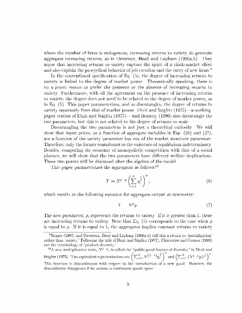
where the number of �rms is endogenous, increasing returns to variety do generate

aggregate increasing returns, as in Devereux, Head and Lapham (1996a,b). They

argue that increasing returns to variety capture the spirit of a thick-market e�ect

and also explain the procyclical behavior of job creation and the entry of new �rms.9

In the conventional speci�cation of Eq. (5), the degree of increasing returns to

variety is linked to the degree of market power. Theoretically speaking, there is

no a-priori reason to prefer the presence or the absence of increasing returns to

variety. Furthermore, with all the agreement on the presence of increasing returns

to variety, the degree does not need to be related to the degree of market power, as

in Eq. (5). This paper parameterizes, and so disentangles, the degree of returns to

variety separately from that of market power. Dixit and Stiglitz (1975)|a working-

paper version of Dixit and Stiglitz (1977)| and Benassy (1996) also disentangle the

two parameters, but this is not related to the degree of returns to scale.

Disentangling the two parameters is not just a theoretical curiosity. We will

show that input prices, as a function of aggregate variables in Eqs. (26) and (27),

are a function of the variety parameter but not of the market structure parameter.

Therefore, only the former contributes to the existence of equilibrium indeterminacy.

Besides, comparing the economy of monopolistic competition with that of a social

planner, we will show that the two parameters have di�erent welfare implications.

These two points will be discussed after the algebra of the model.

This paper parameterizes the aggregator as follows:10

Y = N���

NXi=1

y1�

i

!�

; (6)

which results in the following equation for aggregate output at symmetry:

Y = N�y: (7)

The new parameter, �, represents the returns to variety. If it is greater than 1, there

are increasing returns to variety. Note that Eq. (5) corresponds to the case when �

is equal to �. If it is equal to 1; the aggregator implies constant returns to variety

9Romer (1987) and Devereux, Head and Lapham (1996a,b) call this a return to `specialization'

rather than `variety.' Following the title of Dixit and Stiglitz (1977), Chatterjee and Cooper (1993)

use the terminology of `product diversity.'10A new multiplicative term, N���, is called the \public-good feature of diversity" in Dixit and

Stiglitz (1975). Two equivalent representations are

�PN

i=1N( ���1)y

1�

i

��and

�PN

i=1 (N���yi)

1�

��.

This function is discontinuous with respect to the introduction of a new good. However, the

discontinuity disappears if we assume a continuous goods space.

9

as assumed in Rotemberg and Woodford (1995). They motivate constant returns as

a normalization, but this assumption is a restriction rather than a normalization.

The aggregator is assumed to maximize its pro�t:

� = PY �NXi=1

piyi;

where all price variables are exogenous to the aggregator and the aggregate price

index is de�ned as:11

P = N�(���)

NXi=1

p�

1��1

i

!�(��1)

:

The �rst order condition with respect to yi reduces to a constant-elasticity inverse

demand function:

pi = PN( ���� )�yi

Y

����1

�

: (8)

Note that the new parameter, �; a�ects only the level of the demand without a�ect-

ing its elasticity. Hence the �rst order conditions of the �rms, Eqs. (2) and (3), are

not sensitive to the parameterization of returns to variety.

Besides aggregating di�erentiated goods, macroeconomics has also made it a

convention to scrutinize a symmetric equilibrium under identical technologies of

the �rms. The homogeneity of capital and labor implies the following relations in

equilibrium:

K = Nk; L = Nl; (9)

where K and L denote aggregate capital and aggregate labor, respectively.

2.3 Returns to Scale

Based upon previous discussions on �rms' behavior and aggregation, we now derive

the aggregate reduced-form production function, i.e. an aggregate version of �rms'

technology with a zero-pro�t condition imposed. Aggregation of homogeneous in-

puts in Eq. (9), together with aggregation of outputs as shown in Eq. (7), transforms

the �rms' technologies, Eq. (1), as follows:

Y = N (�� )�K�L1��

� �N��: (10)

11At symmetry, P = 1

N(��1) p. Increasing returns to variety imply that an increase in the number

of �rms leads to a decrease in the price index due to an e�ciency gain. See Feenstra (1994) for an

application to import goods. Existing price indices do not adjust bene�ts to variety: they assume

� = 1.

10

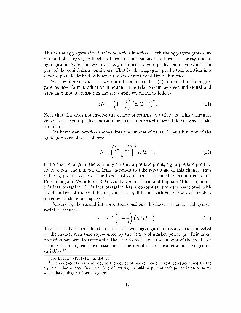
This is the aggregate structural production function. Both the aggregate gross out-

put and the aggregate �xed cost feature an element of returns to variety due to

aggregation. Note that we have not yet imposed a zero-pro�t condition, which is a

part of the equilibrium conditions. That is, the aggregate production function in a

reduced form is derived only after the zero-pro�t condition is imposed.

We now derive what the zero-pro�t condition, Eq. (4), implies for the aggre-

gate reduced-form production function. The relationship between individual and

aggregate inputs transforms the zero-pro�t condition as follows:

�N =

1�

�

!�K�L1��

� : (11)

Note that this does not involve the degree of returns to variety, �. This aggregate

version of the zero-pro�t condition has been interpreted in two di�erent ways in the

literature.

The �rst interpretation endogenizes the number of �rms, N , as a function of the

aggregate variables as follows:

N =

0@�1�

�

��

1A

1

K�L1��: (12)

If there is a change in the economy causing a positive pro�t, e.g. a positive produc-

tivity shock, the number of �rms increases to take advantage of this change, thus

reducing pro�ts to zero. The �xed cost of a �rm is assumed to remain constant.

Rotemberg and Woodford (1995) and Devereux, Head and Lapham (1996a,b) adopt

this interpretation. This interpretation has a conceptual problem associated with

the de�nition of the equilibrium, since an equilibrium with entry and exit involves

a change of the goods space.12

Conversely, the second interpretation considers the �xed cost as an endogenous

variable, that is:

� = N�

1�

�

!�K�L1��

� : (13)

Taken literally, a �rm's �xed cost increases with aggregate inputs and is also a�ected

by the market structure represented by the degree of market power, �. This inter-

pretation has been less attractive than the former, since the amount of the �xed cost

is not a technological parameter but a function of other parameters and exogenous

variables.13

12See Benassy (1991) for the details.13The endogeneity with respect to the degree of market power might be rationalized by the

argument that a larger �xed cost (e.g. advertising) should be paid at each period in an economy

with a larger degree of market power.

11

However, an increase in the �xed cost per �rm is equivalent to job creation on

the intensive margin. That is, output per �rm is proportional to the �xed cost.

Furthermore, over low frequencies of a growing economy, it is reasonable to assume

that �xed costs grow as �rm size grows over time. No papers have argued for this

interpretation seriously, but some follow this interpretation implicitly by assuming

that the number of �rms is constant. If the number of �rms is assumed to be

constant, as in Hornstein (1993), Yun (1996), and Beaudry and Devereux (1995a),

the only way to achieve the zero-pro�t condition is by endogenizing the �xed cost

of a �rm.

As with the speci�cation of the aggregator, there is no a priori reason to prefer

either interpretation. In general, both the �xed cost and the number of �rms may

change. This paper, �rst in the literature, incorporates this generality by de�ning

an additional parameter, " 2 [0; 1], which represents the ratio of the intensive and

extensive margins. Our parameterization postulates the �xed cost and the number

of �rms as follows:14

� =1

�

" 1�

�

!�K�L1��

� #"; (14)

N = �

" 1�

�

!�K�L1��

� #1�"; (15)

where � is an arbitrary constant. This constant a�ects only the level of variables,

but not their percentage deviation. We can interpret the parameter " as one related

with the elasticity of supplying new �rms. Manipulating Eqs. (14) and (15), we have

a constant-elasticity supply schedule,

N " = ��1�";

where � is interpreted as the marginal cost of some specialized resource, e.g. en-

trepreneurial ability, required to create a new �rm. For example, when " = 0, the

supply of entrepreneurial ability is in�nitely elastic at a price of � per unit.

Note that the extreme cases of " = 0 and " = 1 correspond to the two interpreta-

tions in the literature, Eqs. (12) and (13). This paper shows that our generalization

is analytically tractable and gives intuition for the interaction among the various

increasing returns. Before discussing the general case containing the parameter ",

we consider the two extreme cases.

14This parameterization of endogenous �xed costs can be reconciled with that of exogenous �xed

costs, when negative externalities are introduced via �xed costs as in Appendix D. Optimal decision

of �xed cost in industrial-organization literature endogenizes the " parameter, but constant " is

not a bad approximation when time unit if constant.

12

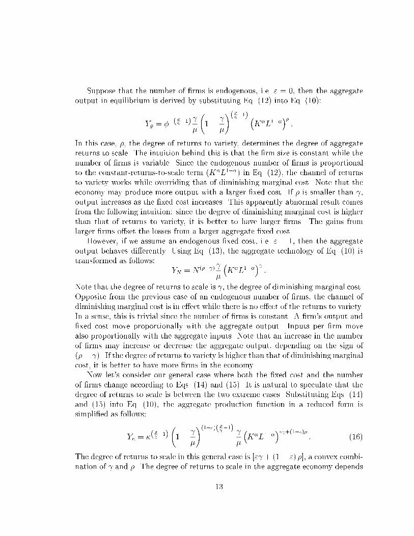
Suppose that the number of �rms is endogenous, i.e. " = 0, then the aggregate

output in equilibrium is derived by substituting Eq. (12) into Eq. (10):

Y� = ��( � �1)

�

1�

�

!( � �1) �K�L1��

��:

In this case, �, the degree of returns to variety, determines the degree of aggregate

returns to scale. The intuition behind this is that the �rm size is constant while the

number of �rms is variable. Since the endogenous number of �rms is proportional

to the constant-returns-to-scale term (K�L1��) in Eq. (12), the channel of returns

to variety works while overriding that of diminishing marginal cost. Note that the

economy may produce more output with a larger �xed cost. If � is smaller than ,

output increases as the �xed cost increases. This apparently abnormal result comes

from the following intuition: since the degree of diminishing marginal cost is higher

than that of returns to variety, it is better to have larger �rms. The gains from

larger �rms o�set the losses from a larger aggregate �xed cost.

However, if we assume an endogenous �xed cost, i.e. " = 1, then the aggregate

output behaves di�erently. Using Eq. (13), the aggregate technology of Eq. (10) is

transformed as follows:

YN = N (�� )

�

�K�L1��

� :

Note that the degree of returns to scale is , the degree of diminishing marginal cost.

Opposite from the previous case of an endogenous number of �rms, the channel of

diminishing marginal cost is in e�ect while there is no e�ect of the returns to variety.

In a sense, this is trivial since the number of �rms is constant. A �rm's output and

�xed cost move proportionally with the aggregate output. Inputs per �rm move

also proportionally with the aggregate inputs. Note that an increase in the number

of �rms may increase or decrease the aggregate output, depending on the sign of

(�� ). If the degree of returns to variety is higher than that of diminishingmarginal

cost, it is better to have more �rms in the economy.

Now let's consider our general case where both the �xed cost and the number

of �rms change according to Eqs. (14) and (15). It is natural to speculate that the

degree of returns to scale is between the two extreme cases. Substituting Eqs. (14)

and (15) into Eq. (10), the aggregate production function in a reduced form is

simpli�ed as follows:

Y� = �(�

�1)

1�

�

!(1�")( � �1)

�

�K�L1��

�" +(1�")�: (16)

The degree of returns to scale in this general case is [" + (1� ") �], a convex combi-

nation of and �. The degree of returns to scale in the aggregate economy depends

13

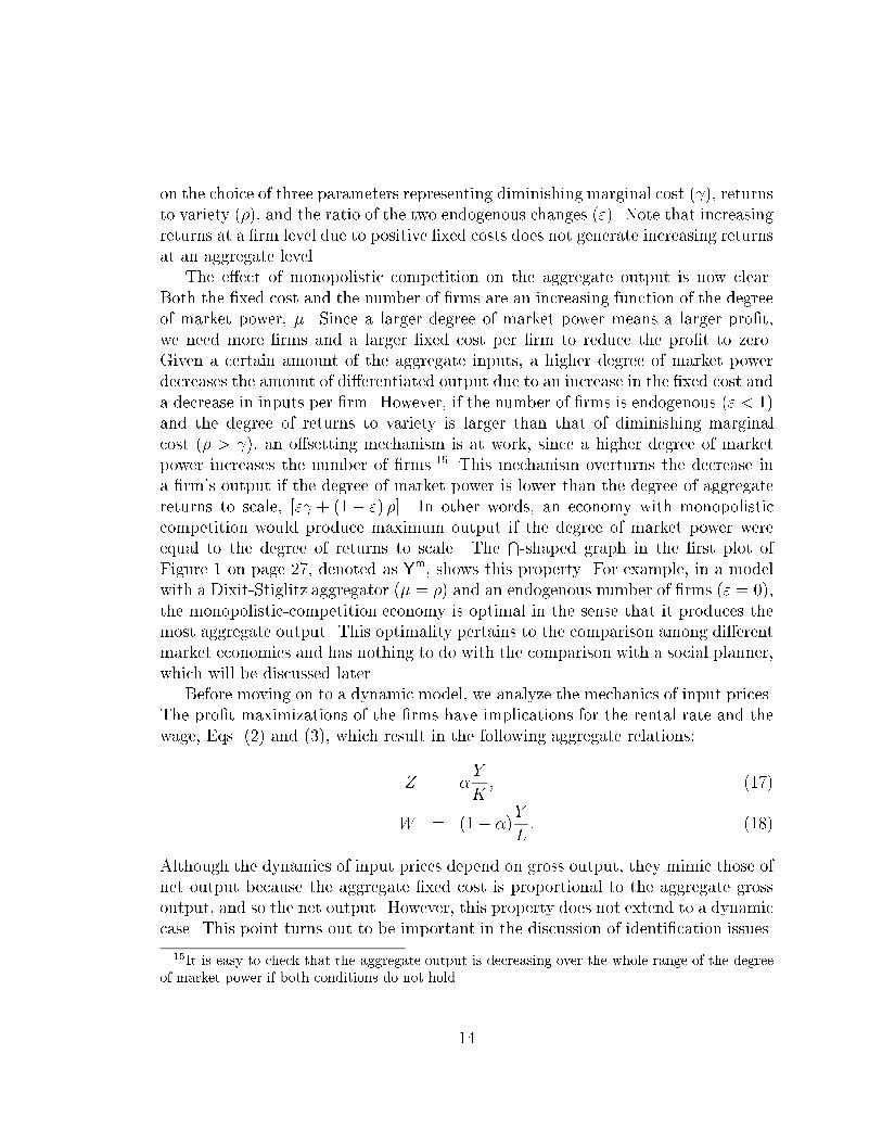
on the choice of three parameters representing diminishing marginal cost ( ), returns

to variety (�), and the ratio of the two endogenous changes ("). Note that increasing

returns at a �rm level due to positive �xed costs does not generate increasing returns

at an aggregate level.

The e�ect of monopolistic competition on the aggregate output is now clear.

Both the �xed cost and the number of �rms are an increasing function of the degree

of market power, �. Since a larger degree of market power means a larger pro�t,

we need more �rms and a larger �xed cost per �rm to reduce the pro�t to zero.

Given a certain amount of the aggregate inputs, a higher degree of market power

decreases the amount of di�erentiated output due to an increase in the �xed cost and

a decrease in inputs per �rm. However, if the number of �rms is endogenous (" < 1)

and the degree of returns to variety is larger than that of diminishing marginal

cost (� > ), an o�setting mechanism is at work, since a higher degree of market

power increases the number of �rms.15 This mechanism overturns the decrease in

a �rm's output if the degree of market power is lower than the degree of aggregate

returns to scale, [" + (1� ") �]. In other words, an economy with monopolistic

competition would produce maximum output if the degree of market power were

equal to the degree of returns to scale. TheT-shaped graph in the �rst plot of

Figure 1 on page 27, denoted as Ym, shows this property. For example, in a model

with a Dixit-Stiglitz aggregator (� = �) and an endogenous number of �rms (" = 0),

the monopolistic-competition economy is optimal in the sense that it produces the

most aggregate output. This optimality pertains to the comparison among di�erent

market economies and has nothing to do with the comparison with a social planner,

which will be discussed later.

Before moving on to a dynamic model, we analyze the mechanics of input prices.

The pro�t maximizations of the �rms have implications for the rental rate and the

wage, Eqs. (2) and (3), which result in the following aggregate relations:

Z = �Y

K; (17)

W = (1� �)Y

L: (18)

Although the dynamics of input prices depend on gross output, they mimic those of

net output because the aggregate �xed cost is proportional to the aggregate gross

output, and so the net output. However, this property does not extend to a dynamic

case. This point turns out to be important in the discussion of identi�cation issues.

15It is easy to check that the aggregate output is decreasing over the whole range of the degree

of market power if both conditions do not hold.

14

2.4 A Dynamic Model

Up to now, neither the size of the �xed cost nor the degree of market power a�ects

the degree of returns to scale. Then, is there no point of introducing monopolistic

competition and the �xed cost in the behavior of returns to scale? Yes, the presence

of the �xed cost does a�ect returns to scale in a dynamic model where adjustments

to zero pro�t are not instantaneous. Note that the static case considered above

is analogous to the Marshallian long run, in that no specialized resource prevents

zero pro�ts from being achieved. Following the same spirit, we interpret a dynamic

case considered below as the Marshallian short run since existing �rms may earn

quasi-rents.

To consider a dynamic case, the aggregate technology without the zero-pro�t

condition imposed, Eq. (10), is rewritten with time subscripts for the variables.

Yt = N(�� )t

�K�

t L1��t

� �N

�t �t: (19)

This structural production function does not directly involve the degree of market

power, �. However, this degree representing the market structure may a�ect the

degree of returns to scale of the aggregate reduced-form production function in a

dynamic model.

Apart from the choice of endogenous variables in a static model, an additional

consideration arises in a dynamic model: how fast does the economy move towards

the state of zero pro�ts? Two extreme cases have been considered in the literature.

In the case of full adjustment, pro�t is zero at every period. This speci�cation is

used in Devereux, Head and Lapham (1996a,b). The short-run dynamics are the

same as that of the static model described in Eqs. (16){(18). The other extreme

is the case of no short-run adjustment. Pro�t is zero only at the steady state, so

the short-run dynamics of the �xed cost and the number of �rms are not a�ected

even if pro�t is not zero in a particular period. Hornstein (1993) and Beaudry and

Devereux (1995a) adopt this speci�cation. In this case, returns to scale are governed

by neither diminishing marginal cost nor returns to variety. They are governed by

the degree of market power, which is a function of the degree of substitution among

di�erentiated goods. These two extreme cases are compared in Chatterjee and

Cooper (1993).

Another contribution in this paper is to generalize the speci�cation of zero pro�ts

by introducing an additional parameter, � 2 [0; 1], representing the speed of adjust-

ments.16 This speed is inversely related to cost of adjustments, e.g. entry and exit.

16Rotemberg and Woodford (1995) is the only example which does not follow one of the two

extreme cases. The calibration corresponds to a very small � of this paper. Optimal decision of

15

We assume that the �xed cost and the number of �rms adjust period by period, but

not fast enough to achieve zero pro�t at every period:17

�t =�~��� ��(1��);

Nt =�~N��

�N (1��);

where�~�; ~N

�guarantees zero pro�t at every period and

���; �N

�guarantees zero

pro�t at the exogenous steady state. Note that no adjustment corresponds to the

case when � = 0, and full adjustment, when � = 1.

Speci�cally, the four variables are de�ned as follows:

~� =1

~�

" 1�

�

!�K�

t L1��t

� #~"; (20)

�� =1

��

" 1�

�

!��K� �L1��

� #�"; (21)

~N = ~�

" 1�

�

!�K�

t L1��t

� #1�~"

; (22)

�N = ��

" 1�

�

!��K� �L1��

� #1��"

: (23)

We will see that only ~", a parameter regarding zero pro�t at every period, matters

for the dynamics of the model. The other parameter, �", a�ects only the steady-state

properties. Alternatively, the speed of adjustments can vary between the �xed cost

and the number of �rms with the assumption that ~" = ��. In this case, the three

parameters are ("; ��; �N). However, this new model is equivalent to our model with

the parameters de�ned as follows:

� = "�� + (1� ")�N ; ~" =��

�"; �" =

1� ��

1� �":

Substituting Eqs. (20){(23) into Eq. (19), the aggregate reduced-form production

function in the dynamic model is as follows:

Yt = �1hK�

t L1��t

i�(~" +(1�~")�)+(1��) � �2

hK�

t L1��t

i�(~" +(1�~")�); (24)

entry and exit in industrial-organization literature endogenizes the � parameter, but constant � is

an approximation under constant time unit. A higher frequency would imply a lower �.17Our speci�cation with an additional parameter preserves the simple one-period nature of the

model. The model becomes intertemporal if we introduce partial adjustments by assuming the

�xed cost and the number of �rms predetermined, as in Ambler and Cardia (1996).

16

where

�1 =�~����1��

�( � �1) 1�

�

 h�K� �L1��

i(1��)(1��")(�� );

�2 =�~����1��

�( � �1) 1�

�

!�~" +(1�~")�

+(1��)

�" +(1��")�

h�K� �L1��

i(1��)(�" +(1��")�):

Note that the two exponent terms in Eq. (24) are di�erent from each other and that

neither of them involves the degree of market power, �. Gross output uctuates

strictly more than the aggregate �xed cost, unless adjustments are instantaneous.

This nonlinear reduced-form production function has such complicated dynamics

that it cannot be compared with the static case. However, in a linearized version of

the dynamic model, the behavior of the variables is comparable to the static model.

In practice, most DSGE papers use a linearized version.

The log-linearized version of Eq. (24) is:

Yt = [� (~" + (1� ~") �) + (1� �)�]��Kt + (1� �) Lt

�; (25)

where xt is the percentage deviation of xt from its steady state. This clearly shows

that market structure a�ects output uctuations in a way indistinguishable from the

two previous sources of increasing returns, diminishing marginal cost and increasing

returns to variety. The degree in the dynamic case is a convex combination of

the degree of the static case in Eq. (16), [~" + (1� ~") �], and the degree of market

power, �. Equivalently, the degree of returns to scale is a convex combination of

the three parameters: the degree of diminishing marginal cost ( ), the degree of

returns to variety (�), and the degree of market power (�). Note that the degree of

returns to scale in the long run, i.e. at the steady state, would be [�" + (1� �") �]

which is di�erent from that of the short run in Eq. (25). This helps explain the

di�erence between low- and high-frequency uctuations, both of which are important

in macroeconomics.

In the extreme case where there is no period-by-period adjustment, the degree

of short-run returns to scale is the degree of market power; the other two param-

eters do not enter at all. The intuition of this extreme case is as follows. Since

aggregate �xed cost does not respond to the change of aggregate inputs, net aggre-

gate output uctuates more than gross aggregate output. Furthermore, the amount

�rms produce relative to the size of the �xed cost depends on the degree of market

power. The result of this extreme case shows that the introduction of diminish-

ing marginal cost in Hornstein (1993) and Beaudry and Devereux (1995a) does not

a�ect the dynamics of the aggregate reduced-form production function. However,

17

this does not mean that the introduction has no in uence on the dynamics of a

general-equilibrium model at all. The degree of diminishing marginal cost a�ects

the dynamics of input prices as follows.

In a dynamic case, the dynamics of the rental rate and the wage are as follows:

Zt = �

�

!�1hK�

t L1��t

i�(~" +(1�~")�)+(1��)

Kt

; (26)

Wt = (1� �)

�

!�1hK�

t L1��t

i�(~" +(1�~")�)+(1��)

Lt

: (27)

Regardless of the assumption about adjustments, the degree of market power does

not a�ect the dynamics of the input prices. The dynamic properties of input prices

are governed by those of gross output rather than net output, since �xed costs and

the number of �rms are exogenous to the �rm's input decision. For example, in

models where the presence of �xed costs is the only source of increasing returns

as in Hornstein (1993) and Rotemberg and Woodford (1995), the introduction of

monopolistic competition and increasing returns does not a�ect the dynamics of

input prices as a function of aggregate inputs.

Note that the exponent term relevant for the input-price dynamics is strictly

smaller than that of the aggregate returns to scale, unless the adjustments are

instantaneous.18 This di�erence has an implication for deriving indeterminacy from

increasing returns to scale, as in Benhabib and Farmer (1994). Since the dynamics

of the input prices are critical for the existence of indeterminacy, all sources of

increasing returns do not contribute to its existence. Of the three sources, the

degree of market power has nothing to do with the existence of indeterminacy.

The bottom line of the model is as follows. The degree of returns to scale

of the aggregate reduced-form production function is a convex combination of three

parameters: the degree of diminishing marginal cost, the degree of returns to variety,

and the degree of market power. The weights depend on the speci�cation of a zero-

pro�t condition. Unless zero pro�t is imposed period by period, the dynamics of

input prices have information independent of the aggregate reduced-form production

function.

18In other words, even if we have the dynamics of output and each input, we do not derive the

dynamics of the input prices. The dynamics of the input prices have some independent implications.

18

3 Implications

This section derives implications of the model and, based upon them, reviews and

critiques existing literature. The model is related to two branches of empirical

literature. A direct implication comes from the behavior of the aggregate reduced-

form production function. The DSGE literature on monopolistic competition uses

a speci�c parameterization of this paper. Our general model in this paper gives a

warning sign to both calibration and estimation approaches. Another implication of

the model involves the works using disaggregate data to identify some parameters.

This paper gives interpretations for the estimates this literature have found, di�erent

from how they used to be interpreted. In addition to these empirical implications,

this paper derives welfare implications. We compare an economy of monopolistic

competition with a social planner's economy and �nd that some previous welfare

results are due to restricted speci�cations.

3.1 Identi�cation with Aggregate Data

To facilitate the discussion of identi�cation issues, we begin by comparing the speci�-

cations of how the existing literature parameterizes the speed of adjustments (�) and

the period-by-period endogeneity between the �xed cost and the number of �rms (~").

For convenience, recall that the degree of returns to scale of the aggregate reduced-

form production function is [� (~" + (1� ~")�) + (1� �)�]. Therefore, this value is

of sole importance in determining the aggregate dynamics of the production func-

tion. The dynamics of input prices are governed by [� (~" + (1� ~")�) + (1� �) ],

the degree of returns to scale of aggregate gross output.

Hornstein (1993) and Beaudry and Devereux (1995a) assume that only the �xed

cost is endogenous and that the adjustment to zero pro�t occurs only at the steady

state. Since the resulting degree of aggregate returns is �, diminishing marginal

cost and increasing returns to variety do not a�ect the dynamics of the aggregate

reduced-form production function. However, this does not mean that, in a particular

general-equilibrium model, the dynamics of output depend only on the degree of

market power. Since the dynamics of input prices depend on diminishing marginal

cost and returns to variety, they also a�ect output in a general-equilibrium model.19

In Rotemberg and Woodford (1995), the endogenous variable is not the �xed cost

but the number of �rms. However, this does not make much di�erence because their

calibrated speed of adjustments is very low, a small �. If the responses of the number

19For example, the second and the third cases of Hornstein (1993) do not produce the same

results even if the only di�erence between the two cases lies in the degree of diminishing marginal

cost.

19

~"n� 0 1

0 Rotemberg and Woodford (1995) Devereux, Head and Lapham (1996a,b,c)

1Hornstein (1993)

Beaudry and Devereux (1995a)

Table 1: Examples of Speci�cation

of �rms happen only at the steady state, a zero �, then di�erent assumptions on

endogeneity do not make any di�erence at all.

The endogeneity of the number of �rms matters if the zero-pro�t condition is

imposed period by period, as in Devereux, Head and Lapham (1996a,b,c). The

dynamics of both output and input prices depend on the degree of returns to variety.

The degree of diminishing marginal cost and that of market power do not a�ect

the properties of the variables, as far as the percentage deviations are concerned.

Table 1 summarizes the speci�cations. The �rst column corresponds to a model

where adjustments to zero pro�t occur only at the steady state.20 The second

column contains the static version of this paper, where returns to variety matters.

The �rst and the second rows correspond to models of endogenous number of �rms

and endogenous �xed cost, respectively.

Discussion of econometric issues such as identi�cation naturally involves the

speci�cation of an error structure. A convention is to interpret the productivity

shocks as a random variable. Accordingly, this section restores the notation for

productivity shocks, At. Note that identi�cation issues can be discussed only in

the context of a speci�c model and available data. From the calibration point of

view, identi�cation issues are interpreted as follows. If the model is not identi�ed,

di�erent parameter calibrations may result in the same model.

Suppose that our model is the aggregate reduced-form production function with

exogenous steady states and that we have aggregate data on output, capital and la-

bor. Augmenting the linearized aggregate reduced-form production function, Eq. (25),

with productivity shocks as an error structure, we have:

Yt = [� (~" + (1� ~") �) + (1� �)�]

�Kt + (1� �) Lt +

1

At

!:

Using the aggregate data, we can draw inferences about the share parameter, �, and

the aggregate returns to scale, [� (~" + (1� ~") �) + (1� �)�]. The three parameters

representing the degrees are not identi�ed separately. From the calibration point

20Rotemberg and Woodford (1995) is included in this category since � is very small, even if not

exactly zero.

20

of view, di�erent parameter calibrations may result in the same aggregate returns

to scale. For example, the dynamic properties of Rotemberg and Woodford (1995)

with slow period-by-period adjustments, i.e. a small nonzero �, can be replicated

by another economy where adjustments occur only at the steady state, i.e. zero

�. Since the �xed cost is exogenous (~" = 0), the degree of aggregate returns to

scale is [��+ (1� �)�]. Because the degree of returns to variety is normalized to

1, an appropriate decrease in the degree of market power by � (�� 1) is the only

modi�cation necessary in the new economy without any short-run adjustments. The

dynamic behavior of all the aggregate variables, except for the gross output and the

number of �rms, is the same as that of the original model.

More aggregate data may solve the identi�cation problem. Data on the �xed cost

or the number of �rms would be helpful. However, it is not likely that we can get

measures of these two variables, consistent with this paper. Now suppose that we

have additional data on the rental rate or the wage and that the model also includes

the appropriate input-price equation, Eq. (26) or (27). The new model identi�es

another linear combination of parameters, [� (~" + (1� ~") �) + (1� �) ].21 This

is di�erent from the degree of aggregate returns and so the model identi�es two

parameters, unless adjustments are instantaneous. For example, the two free pa-

rameters estimated in Kim (1996) are and �, both of which are identi�ed for the

following reason. Since adjustments are assumed to occur only at the steady state,

the degree of aggregate returns is � and the dynamics of input prices are governed

by . Additional data on the interest rate provide information on the rental rate

and so is also identi�ed.

Considering the identi�cation problems, one may wonder why we care about

various increasing returns separately. This question will be answered when the

market economy is compared with a social planner. We will show that di�erent

increasing returns have di�erent normative implications. Before comparing with a

social planner, we review the literature using disaggregate data to identify some

parameters of the model.

3.2 Interpretation of Disaggregate Data

Recall that the aggregate economy has been derived from a �rm's problem. If we

interpret a �rm as a particular sector of the economy, the data disaggregated to the

sectoral level have implications on the state of the economy. Two related literatures

apply this interpretation. Here, we evaluate the implications of these literatures by

21Note that the replication of Rotemberg and Woodford (1995) in the previous paragraph does

not change input-price dynamics. Since both and � are equal to 1, the change in � does not

change the dynamics.

21

using our general speci�cation of increasing returns in a monopolistic-competition

model.

Firm's �rst order conditions are the starting point of testing the joint hypothesis

of perfectly competitive markets and constant returns to scale, as in Hall (1996, 1998,

1990). However, compared with the model in this paper, they do not incorporate

a zero-pro�t condition. Since it is assumed that there are no �xed costs, there is

no di�erence between the structural production function and its reduced form. The

log-linearized production function is:

dyit

yit= i

�i

dkit

kit+ (1� �i)

dlit

lit

!+dAit

Ait

:

The analysis of Hall (1986, 1988, 1990) is based on the measurement of productivity

growth in Solow (1957). Calculation of the Solow residual requires the revenue share:

sR =Wtlit

pityit: (28)

Without zero-pro�t conditions or �xed costs, the revenue share is equal to i�(1��i).

Therefore, the Solow residual is:

dyit

yit� sR

dlit

lit� (1� sR)

dkit

kit= (�� 1)sR

dlit

lit�dkit

kit

!+ ( i � 1)

dkit

kit+dAit

Ait

:

This is the basis of testing for the joint hypothesis of perfect competition (� = 1)

and constant returns to scale ( i = 1).

Hall (1990) proposes a way to di�erentiate diminishingmarginal cost frommarket

power. He de�nes a new share as follows:

sC =Wtlit

Ztkit +Wtlit:

This is called the cost share, since it is the share of labor input in total cost, rather

than in total revenue as in Eq. (28). Note that it is equal to the share parameter,

(1��i), regardless of increasing returns and market power. The cost-based residual

is as follows:

dyit

yit� sC

dlit

lit� (1� sC)

dkit

kit= ( i � 1)

sC

dlit

lit+ (1� sC)

dkit

kit

!+dAit

Ait

:

Unlike the Solow residual, the cost-based residual can provide information only on

increasing returns.22 This algebra lets Hall (1990) conclude that his evidence points

in the direction of increasing returns, presumably coupled with market power.

22The similar results for the Solow residual and the cost-based residual support the absence of

pro�ts in Hall (1990). Note that a zero-pro�t condition is not imposed.

22

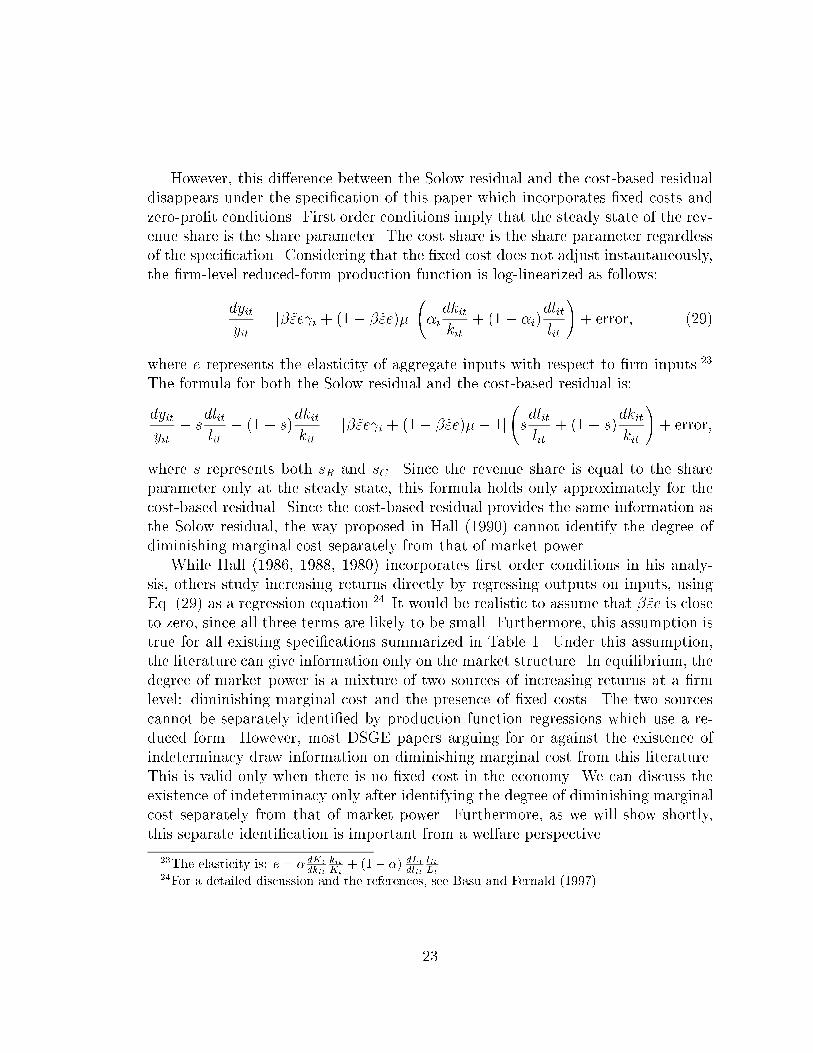
However, this di�erence between the Solow residual and the cost-based residual

disappears under the speci�cation of this paper which incorporates �xed costs and

zero-pro�t conditions. First order conditions imply that the steady state of the rev-

enue share is the share parameter. The cost share is the share parameter regardless

of the speci�cation. Considering that the �xed cost does not adjust instantaneously,

the �rm-level reduced-form production function is log-linearized as follows:

dyit

yit= [�~"e i + (1� �~"e)�]

�i

dkit

kit+ (1� �i)

dlit

lit

!+ error; (29)

where e represents the elasticity of aggregate inputs with respect to �rm inputs.23

The formula for both the Solow residual and the cost-based residual is:

dyit

yit� s

dlit

lit� (1� s)

dkit

kit= [�~"e i + (1� �~"e)�� 1]

sdlit

lit+ (1� s)

dkit

kit

!+ error;

where s represents both sR and sC . Since the revenue share is equal to the share

parameter only at the steady state, this formula holds only approximately for the

cost-based residual. Since the cost-based residual provides the same information as

the Solow residual, the way proposed in Hall (1990) cannot identify the degree of

diminishing marginal cost separately from that of market power.

While Hall (1986, 1988, 1980) incorporates �rst order conditions in his analy-

sis, others study increasing returns directly by regressing outputs on inputs, using

Eq. (29) as a regression equation.24 It would be realistic to assume that �~"e is close

to zero, since all three terms are likely to be small. Furthermore, this assumption is

true for all existing speci�cations summarized in Table 1. Under this assumption,

the literature can give information only on the market structure. In equilibrium, the

degree of market power is a mixture of two sources of increasing returns at a �rm

level: diminishing marginal cost and the presence of �xed costs. The two sources

cannot be separately identi�ed by production function regressions which use a re-

duced form. However, most DSGE papers arguing for or against the existence of

indeterminacy draw information on diminishing marginal cost from this literature.

This is valid only when there is no �xed cost in the economy. We can discuss the

existence of indeterminacy only after identifying the degree of diminishing marginal

cost separately from that of market power. Furthermore, as we will show shortly,

this separate identi�cation is important from a welfare perspective.

23The elasticity is: e = � dKt

dkit

kitKt

+ (1� �) dLt

dlit

litLt

.24For a detailed discussion and the references, see Basu and Fernald (1997).

23

3.3 Comparison with a Social Planner

A basic issue of welfare economics is whether a market solution will yield the social

optimum or not. Unlike the case of monopolistic competition, the zero-pro�t con-

dition is not binding for a social planner. So the planner's problem is static in the

sense that there is no concern about the speed of adjustments. For ease of compar-

ison, adjustments to zero pro�ts are assumed to be instantaneous in the economy

of monopolistic competition, i.e. � = 1, and so time subscripts are suppressed. The

behavior of the market economy is summarized as follows:

�market =

1�

�

!" �K�L1��

�" ;

Nmarket =

1�

�

! 1�" �

K�L1���1�"

;

Y market =

�

1�

�

!(1�")( � �1) �K�L1��

�" +(1�")�;

where the level parameter, �, is normalized to 1 in the original equations, Eq. (14),

(15) and (16). The superscripts of `market' denote the market economy of monop-

olistic competition.

Note that the planner's optimization problem with respect to the �xed cost is

not well-de�ned. For the planner, it is optimal to decrease the �xed cost as close

to zero as possible. So the welfare issues are considered only under the assumption

that the social planner is not allowed to control the �xed cost. Given a process of

the �xed cost, the number of �rms in an economy is chosen by the social planner

whose objective is:

maxN

hN (�� )

�K�L1��

� �N��market

i:

Due to the partial-equilibrium setup of this paper, it is natural for the social plan-

ner to consider aggregate capital and labor as exogenous.25 Note that the market

structure a�ects the planner's problem only through the exogenous process of the

�xed cost. For this problem to be well de�ned, we assume that � > . Under this

assumption, the number of �rms has two o�setting e�ects on the aggregate out-

put. An increase in the number of �rms increases both aggregate gross output and

aggregate �xed cost.

25This problem is di�erent from that of Dixit and Stiglitz (1977) in that the cost function is

parameterized and that the utility function is not introduced. This makes it easy to consider

monopolistic competition and increasing returns simultaneously.

24

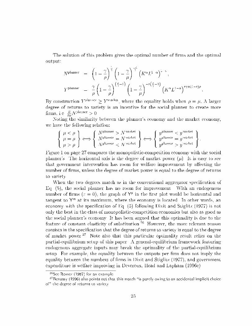
The solution of this problem gives the optimal number of �rms and the optimal

output:

Nplanner =

1�

�

! 1 1�

�

!�" �

K�L1���1�"

;

Y planner =

�

1�

�

!( � �1) 1�

�

!�"( � �1) �

K�L1���" +(1�")�

:

By construction Y planner� Y market, where the equality holds when � = �: A larger

degree of returns to variety is an incentive for the social planner to create more

�rms, i.e. @@�Nplanner > 0.

Noting the similarity between the planner's economy and the market economy,

we have the following relation:8><>:

� < �

� = �

� > �

9>=>;()

8><>:

Nplanner > Nmarket

Nplanner = Nmarket

Nplanner < Nmarket

9>=>;()

8><>:

yplanner < ymarket

yplanner = ymarket

yplanner > ymarket

9>=>; :

Figure 1 on page 27 compares the monopolistic-competition economy with the social

planner's. The horizontal axis is the degree of market power (�). It is easy to see

that government intervention has room for welfare improvement by a�ecting the

number of �rms, unless the degree of market power is equal to the degree of returns

to variety.

When the two degrees match as in the conventional aggregator speci�cation of

Eq. (5), the social planner has no room for improvement. With an endogenous

number of �rms (" = 0), the graph of Yp in the �rst plot would be horizontal and

tangent to Ym at its maximum, where the economy is located. In other words, an

economy with the speci�cation of Eq. (5) following Dixit and Stiglitz (1977) is not

only the best in the class of monopolistic-competition economies but also as good as

the social planner's economy. It has been argued that this optimality is due to the

feature of constant elasticity of substitution.26 However, the more relevant reason

consists in the speci�cation that the degree of returns to variety is equal to the degree

of market power.27 Note also that this particular optimality result relies on the

partial-equilibrium setup of this paper. A general-equilibrium framework featuring

endogenous aggregate inputs may break the optimality of the partial-equilibrium

setup. For example, the equality between the outputs per �rm does not imply the

equality between the numbers of �rms in Dixit and Stiglitz (1977), and government

expenditure is welfare improving in Devereux, Head and Lapham (1996c).

26See Romer (1987) for an example.27Benassy (1996) also points out that this match \is purely owing to an accidental implicit choice

of" the degree of returns to variety.

25

4 Further research

Based on the critical review of the literature, empirical work to identify the parame-

ters needs to be done. Enough data both at aggregate and disaggregate levels might

enable the identi�cation of all the parameters in this paper. The issue is how to �nd

a measure, say of the number of �rms, relevant to this paper. As to the model, the

speci�cation of endogenous �xed costs needs further analysis. It is more appealing if

we have a model which explains how the �xed cost changes endogenously in response

to the change in exogenous variables. The literature on R&D with entry and exit

can be a starting point. Another topic that deserves attention is to include materials

as an input to the technology. Such extension makes the aggregation in an imper-

fectly competitive economy less straightforward, since it involves value added rather

than gross output. Furthermore, it might change some results regarding returns to

scale.28

28See, for example, Hall (1986, 1988, 1990), Rotemberg and Woodford (1995), and Basu and

Fernald (1997).

26

Agg

rega

te O

utpu

t

γ εγ+(1−ε)ρ ρ

Ym

Yp

Num

ber

of F

irms

ργ

Nm

Np

Out

put p

er F

irm

ργ

ym

yp

Degree of Market Power (µ)

Figure 1: Comparison with a Social Planner

27

A External Increasing Returns

Here we suppose that externalities come from inputs, rather than outputs. The

technology of the �rms without externalities, Eq. (1), is rewritten for ease of com-

parison:29

y =�k�l1��

� � �:

Input externalities have been parameterized in two di�erent ways.

If average inputs a�ect the output of �rms, their technology is:

y =�k�l1��

� ��k��l1���� � �;

where �k and �l are average inputs and � denotes the degree of externalities. Following

the same procedure of the aggregation and the zero-pro�t condition, the degree of

aggregate returns to scale in a static model is [~" ( + �) + (1� ~") �]. Note that

externalities via average inputs change the degree of diminishing marginal cost from

to ( + �), without any change in the degree of returns to variety. In a dynamic

case, since the relative size of �xed costs depends on the internal increasing returns

only, the e�ect of market structure is magni�ed by a factor of +� . That is, the

returns to scale in our most general speci�cation is,

� [~" ( + �) + (1� ~") �] + (1� �)

" + �

!�

#:

Production externalities may come through total inputs as follows:

y =�k�l1��

� �K�L1��

��� �;

where K and L denote total capital and labor in the economy. Such externalities

magnify not only the degree of diminishing marginal cost but also that of returns

to variety by a factor of +� . The degree of market power is magni�ed, too. The

degree of returns to scale is, + �

![� (~" + (1� ~") �) + (1� �)�] :

The above algebra shows that a model with external increasing returns and one

with internal increasing returns can replicate the dynamic properties of each other,

subject to the following quali�cation.30 The degree of returns to variety and the

degree of market power should be changed appropriately. For example, if internal

returns are replaced with external returns, the degree of market power in a new

model should be reduced to (� ), the old degree of market power divided by the

degree of internal returns.

29In the Appendix, all subscripts denoting �rm and time are omitted.30This equivalence is also explained in Benhabib and Farmer (1994).

28

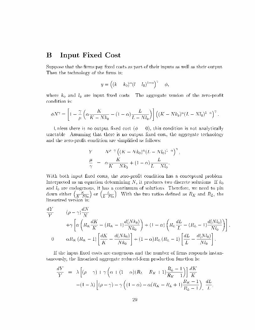
B Input Fixed Cost

Suppose that the �rms pay �xed costs as part of their inputs as well as their output.

Then the technology of the �rms is:

y =�(k � k0)

�(l � l0)1��

� � �;

where k0 and l0 are input �xed costs. The aggregate version of the zero-pro�t

condition is:

�N =

"1�

�

��

K

K �Nk0+ (1� �)

L

L�Nl0

�# �(K �Nk0)

�(L�Nl0)1��

� :

Unless there is no output �xed cost (� = 0), this condition is not analytically

tractable. Assuming that there is no output �xed cost, the aggregate technology

and the zero-pro�t condition are simpli�ed as follows:

Y = N�� �(K �Nk0)

�(L�Nl0)1��

� ;

�

= �

K

K �Nk0+ (1� �)

L

L�Nl0:

With both input �xed costs, the zero-pro�t condition has a conceptual problem.

Interpreted as an equation determining N , it produces two discrete solutions. If k0and l0 are endogenous, it has a continuum of solutions. Therefore, we need to pin

down either�

KK�Nk0

�or�

LL�Nl0

�. With the two ratios de�ned as RK and RL, the

linearized version is:

dY

Y= (�� )

dN

N

+

"�

RK

dK

K� (RK � 1)

d(Nk0)

Nk0

!+ (1� �)

RL

dL

L� (RL � 1)

d(Nl0)

Nl0

!#;

0 = �RK (RK � 1)

"dK

K�d(Nk0)

Nk0

#+ (1� �)RL (RL � 1)

"dL

L�d(Nl0)

Nl0

#:

If the input �xed costs are exogenous and the number of �rms responds instan-

taneously, the linearized aggregate reduced-form production function is:

dY

Y= �

�(�� ) +

�� + (1� �)(RL � RK + 1)

RL � 1

RK � 1

��dK

K

+(1� �)

�(�� ) +

�(1� �) + �(RK �RL + 1)

RK � 1

RL � 1

��dL

L;

29

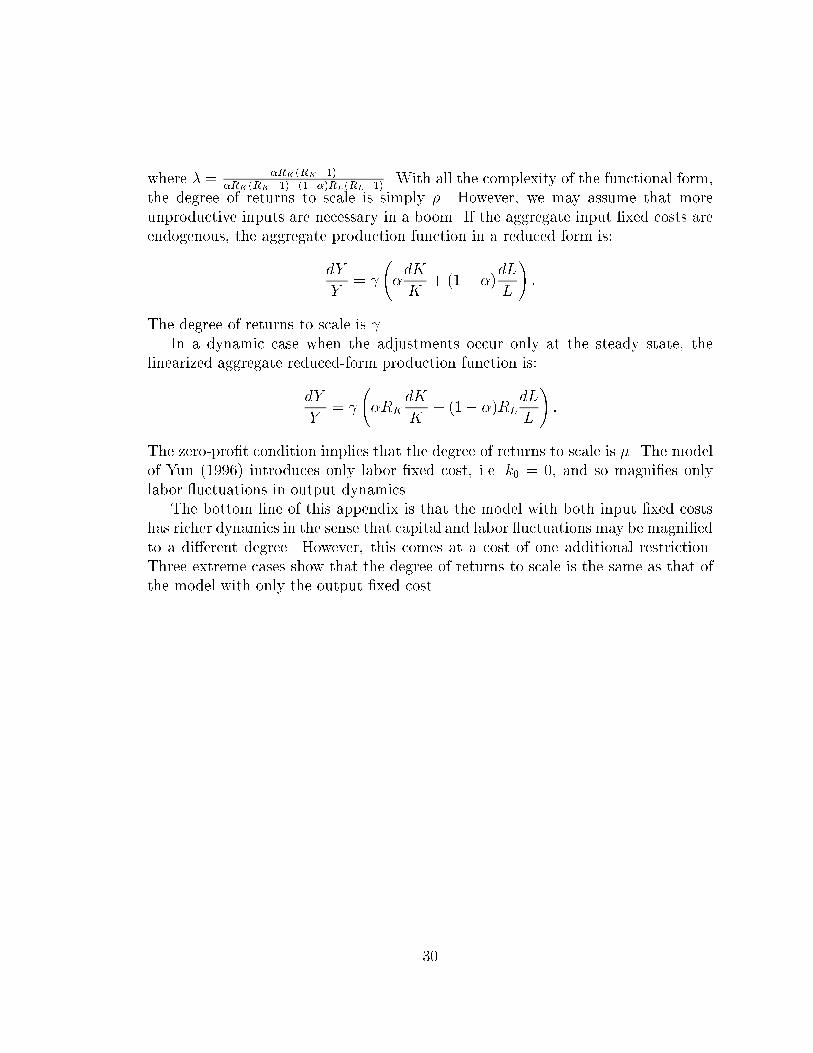
where � = �RK(RK�1)

�RK(RK�1)+(1��)RL(RL�1). With all the complexity of the functional form,

the degree of returns to scale is simply �. However, we may assume that more

unproductive inputs are necessary in a boom. If the aggregate input �xed costs are

endogenous, the aggregate production function in a reduced form is:

dY

Y=

�dK

K+ (1� �)

dL

L

!:

The degree of returns to scale is .

In a dynamic case when the adjustments occur only at the steady state, the

linearized aggregate reduced-form production function is:

dY

Y=

�RK

dK

K+ (1� �)RL

dL

L

!:

The zero-pro�t condition implies that the degree of returns to scale is �. The model

of Yun (1996) introduces only labor �xed cost, i.e. k0 = 0, and so magni�es only

labor uctuations in output dynamics.

The bottom line of this appendix is that the model with both input �xed costs

has richer dynamics in the sense that capital and labor uctuations may be magni�ed

to a di�erent degree. However, this comes at a cost of one additional restriction.

Three extreme cases show that the degree of returns to scale is the same as that of

the model with only the output �xed cost.

30

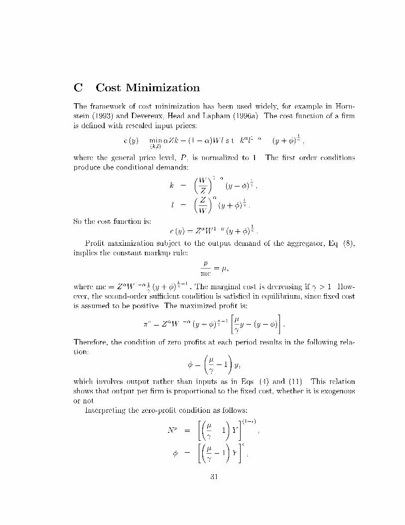
C Cost Minimization

The framework of cost minimization has been used widely, for example in Horn-

stein (1993) and Devereux, Head and Lapham (1996a). The cost function of a �rm

is de�ned with rescaled input prices:

c (y) = min(k;l)

�Zk + (1� �)Wl s.t. k�l1�� = (y + �)1 ;

where the general price level, P , is normalized to 1. The �rst order conditions

produce the conditional demands:

k =

�W

Z

�1��

(y + �)1 ;

l =

�Z

W

��(y + �)

1 :

So the cost function is:

c (y) = Z�W 1�� (y + �)1 :

Pro�t maximization subject to the output demand of the aggregator, Eq. (8),

implies the constant markup rule:

p

mc= �;

where mc = Z�W 1�� 1 (y + �)

1 �1: The marginal cost is decreasing if > 1. How-

ever, the second-order su�cient condition is satis�ed in equilibrium, since �xed cost

is assumed to be positive. The maximized pro�t is:

�� = Z�W 1�� (y + �)1 �1

"�

y � (y + �)

#:

Therefore, the condition of zero pro�ts at each period results in the following rela-

tion:

� =

�

� 1

!y;

which involves output rather than inputs as in Eqs. (4) and (11). This relation

shows that output per �rm is proportional to the �xed cost, whether it is exogenous

or not.

Interpreting the zero-pro�t condition as follows:

N� =

" �

� 1

!Y

#(1��);

� =

" �

� 1

!Y

#�;

31

we transform the conditional demands and the cost function into an aggregate ver-

sion as follows:

K =

�W

Z

�1��

�Y� + 1��

� ; (30)

L =

�Z

W

���Y

� + 1��

� ; (31)

C (Y ;N(Y ); �(N)) = Z�W 1���Y� + 1��

� ;

where � =(� )

1

(� �1)(1��)( 1 � 1

�). The constant markup rule is expressed as follows:

p

MC= �; (32)

where p =h�

�

� 1

�Yi(1��)( ��1� )

and MC = Z�W 1�� 1

(� )1�

(� �1)(1��)

1�

Y�1�

. MC is not

the aggregate marginal cost but just a name for the aggregate counterpart of the

�rm's marginal cost. Note that the inverse of the markup is equal to @@YC (Y ;N; �)

evaluated at the zero-pro�t condition, not to d

dYC (Y ;N(Y ); �(Y )).

Eqs. (30){(32) are a complete description of the economy. Solving for Y as a

function of K and L, we have:

Y =���1K�L1��

�( � + 1��� )

�1

:

The degree of returns to scale is the weighted harmonic average of the degree of

diminishing marginal cost and that of returns to variety. The input prices are:

Z =Y

K;

W =Y

L:

This shows that our results on input prices in a static model are robust to the choice

of the framework.

32

D Fixed Cost Externalities

In the static case, both the �xed cost and the number of �rms are endogenous and

so the degree of returns to scale is a convex combination of the degree of diminishing

marginal cost and that of returns to variety. This appendix shows that the static

model is equivalent to two models where the �xed cost is exogenous and only the

number of �rms is endogenous, i.e. " = 0. That is, aggregate output and the number

of �rms follow Eqs. (10) and (12), rewritten here for convenience.

Y = N (�� )�K�L1��

� �N��;

N =

0@�1�

�

��

1A

1

K�L1��:

Instead of endogenous �xed costs, each model introduces an assumption about �xed

cost externalities. The new parameters, � and �, represent the external diseconomies

such as congestion e�ects.

First, external diseconomies are assumed to a�ect the �xed cost as follows:

� = �1Y�; (33)

where � 2 [0; 1]. An increase in aggregate output would increase the �xed cost per

�rm, less than proportionately. Combining Eq. (33) with the above two equations,

the equilibrium aggregate output is:

Y =��K�L1��

�( � + 1��

� )�1

;

where � = ��(�� � )1

�

�

� 1��1�

�

�( �� � ). The degree of returns to scale is a harmonic

average of the degree of diminishing marginal cost and that of returns to variety.

Alternatively, negative externalities is assumed with respect to the number of

�rms as follows:

� = �2N�;

where � 2 [0;1). An increase in the number of �rms would increase the �xed cost

per �rm, possibly more than proportionately. The same algebra shows that the

equilibrium output is:

Y = ��K�L1��

�[( ��+ ) +(

�+ )�];

where � = ��( �� �+ )2

�1�

�

�( �� �+ )�1� �

��+

2

�1�

�

�

�+

�. As the degree of external-

ity (�) grows from 0 to 1, the degree of returns to scale moves from the degree of

returns to variety (�) to the degree of diminishing marginal cost ( ).

33

References

[1] Ambler, Steve and Emanuela Cardia (1996), \The Cyclical Behavior of Wages

and Pro�ts under Imperfect Competition," mimeo, University of Montreal.

[2] d'Aspremont, Claude, Rodolphe Dos Santos Ferreira, and Louis-Andre Gerard-

Varet (1996), \On the Dixit-Stiglitz Model of Monopolistic Competition,"

American Economic Review, 86(3), 623{629.

[3] Basu, Susanto and John G. Fernald (1997), \Returns to Scale in U.S. Produc-

tion: Estimates and Implications," forthcoming in Journal of Political Econ-

omy.

[4] Beaudry, Paul and Michael B. Devereux (1995a), \Money and the Real Ex-

change Rate with Sticky Prices and Increasing Returns," Carnegie-Rochester

Conference Series on Public Policy, 43, 55{102.

[5] Beaudry, Paul and Michael B. Devereux (1995b), \Monopolistic Competition,

Price Setting and the E�ects of Real and Monetary Shocks," mimeo, University

of British Columbia.

[6] Benassy, Jean-Pascal (1991), \Monopolistic Competition," in W. Hidebrand

and H. Sonnenschein, eds., Handbook of Mathematical Economics, Volume IV,

1997{2045.

[7] Benassy, Jean-Pascal (1996), \Taste for Variety and Optimum Production Pat-

terns in Monopolistic Competition," Economics Letters, 52, 41{47.

[8] Benhabib, Jess and Roger E. A. Farmer (1994), \Indeterminacy and Increasing

Returns," Journal of Economic Theory, 63, 19{41.

[9] Blanchard, Olivier J. and Nobuhiro Kiyotaki (1987), \Monopolistic Competi-

tion and the E�ects of Aggregate Demand," American Economic Review, 77(4),

647{666.

[10] Chatterjee, Satyajit and Russell W. Cooper (1993), \Entry and Exit, Product

Variety and the Business Cycle," NBER WP #4562.

[11] Devereux, Michael B., Allen C. Head, and Beverly J. Lapham (1996a), \Mo-

nopolistic Competition, Increasing Returns, and the E�ects of Government

Spending," Journal of Money, Credit, and Banking, 28(2), 233{254.

34

[12] Devereux, Michael B., Allen C. Head, and Beverly J. Lapham (1996b), \Aggre-

gate Fluctuations with Increasing Returns to Specialization and Scale," Journal

of Economic Dynamics and Control, 20, 627{656.

[13] Devereux, Michael B., Allen C. Head, and Beverly J. Lapham (1996c), \Govern-

ment Spending and Welfare with Returns to Specialization," mimeo, University

of British Columbia and Queen's University.

[14] Dixit, Avinash K. and Joseph Stiglitz (1975), \Monopolistic Competition and

Optimum Product Diversity," University of Warwick WP #64.

[15] Dixit, Avinash K. and Joseph Stiglitz (1977), \Monopolistic Competition and

Optimum Product Diversity," American Economic Review, 67, 297{308.

[16] Feenstra, Robert C. (1994), \New Product Varieties and the Measurement of

International Prices," American Economic Review, 84(1), 157{177.

[17] Hairault, Jean-Olivier and Franck Portier (1993), \Money, New-Keynesian

Macroeconomics and the Business Cycle," European Economic Review, 37,

1533{1568.

[18] Hall, Robert E. (1986), \Market Structure and Macroeconomic Fluctuations,"

Brookings Papers on Economic Activity, 2, 285{322.

[19] Hall, Robert E. (1988), \The Relation between Price and Marginal Cost in U.S.

Industry," Journal of Political Economy, 96, 921{947.

[20] Hall, Robert E. (1990), \Invariance Properties of Solow's Productivity Resid-

ual," in P. Diamond, ed., Growth, Productivity, Unemployment, Cambridge:

MIT Press, 71{112.

[21] Hornstein, Andreas (1993), \Monopolistic Competition, Increasing Returns to

Scale and the Importance of Productivity Shocks," Journal of Monetary Eco-

nomics, 31, 299{316.

[22] Kim, Jinill (1996), \Monetary Policy in a Stochastic Equilibrium Model with

Real and Nominal Rigidities," mimeo, Yale University.

[23] Matsuyama, Kiminori (1995), \Complementarities and Cumulative Processes

in Models of Monopolistic Competition," Journal of Economic Literature, 33,

701{729.

35

[24] Romer, Paul M. (1987), \Growth Based on Increasing Returns Due to Special-

ization," American Economic Review Papers and Proceedings, 77(2), 56{62.

[25] Rotemberg, Julio J. and Michael Woodford (1995), \Dynamic General Equilib-

rium Models with Imperfectly Competitive Product Markets," in Frontiers of

Business Cycle Research, Thomas F. Cooley (ed.), Princeton University Press,

Princeton, NJ.

[26] Solow, Robert M. (1957), \Technical Change and the Aggregate Production

Function," Review of Economics and Statistics, 39, 312{320.

[27] Yun, Tack (1996), \Nominal Price Rigidity, Money Supply Endogeneity, and

Business Cycles," Journal of Monetary Economics, 37, 345{370.

36