Thwarting Adversaries with Unpredictability:Massive-scale Game-Theoretic Algorithms for Real-world Security Deployments

by

Manish Jain

A Dissertation Presented to theFACULTY OF THE USC GRADUATE SCHOOLUNIVERSITY OF SOUTHERN CALIFORNIA

In Partial Fulfillment of theRequirements for the DegreeDOCTOR OF PHILOSOPHY

(COMPUTER SCIENCE)

August 2013

Copyright 2013 Manish Jain

Acknowledgments

Today, I stand on the advise and support of many people. My research style, skills and direction

has been forged after many discussions with my advisor, colleagues, friends and family. I would

like to give a special thanks to my advisor Milind Tambe without whom I would not be the

researcher I am today and this thesis would probably be non-existent. Milind, I thank you for

your unending dedication to my progress and success, and for the countless hours you have spent

on having discussions with me, advising me, debating with me, correcting my unpolished drafts

and advertising my finished results. I have thoroughly enjoyed my PhD process, and a whole

lot of credit goes to just you. You taught me what it meant to do research. You gave me the

opportunity to work on a problem where I could see my research in action – a thought that still

gives me goosebumps. I appreciate and thank you for how you sought out opportunities for awards,

presentations and collaborations for me. I admire you for helping me grow as a presenter of my

work. I still remember the rather embarrassing presentation at the Preference Handling Workshop

at AAAI, 2008 when I was so nervous that I ran through my slides in about 10 minutes in a 25

minute slot – it has been a journey of progress since then. I also praise you for your efforts you put

to maintain an active social life in the group with our coffees, lunches, dinners, boat cruises and

retreats, and how you keep engaged with the alumni of our research group. I cannot even begin to

ii

enumerate the things that I have learnt from you and would hopefully be emulating in my research

career as I move forward.

I would also like to thank other members of my thesis committee, namely, Fernando Ordonez,

Vincent Conitzer, Bhaskar Krishnamachari and Mathew McCubbins for their helpful feedback and

guidance. A special thanks to Fernando, since he was a tremendous guide to me when I started

my research on developing scalable algorithms. You introduced me to large-scale optimization

techniques of Operations Research, a tool that I have used extensively throughout my thesis work.

We have collaborated since 2008 and I hope that our collaboration extends much further. Similarly,

I would like to especially thank Vince for all his help through the years. You have been a part of

multiple research efforts that have constituted my work, and this thesis would definitely not be in

its current shape without you.

I would also like to thank the many collaborators I have had over the years. Apart from Milind,

Fernando and Vince, I have been fortunate enough to work along with many researchers. I thank

all of them whole-heartedly. This lists includes Sarit Kraus, Makoto Yokoo, Kevin Leyton-Brown,

Christopher Kiekintveld, Matthew E. Taylor, Bo An, Albert Xin Jiang, James Pita, Jason Tsai, Eric

Shieh, Ondrej Vanek, Zhengyu Yin, Branislav Bosansky, Michal Pechoucek, Dmytrov Korzhyk,

Rong Yang, Erim Kardes and Jun-young Kwak, among others. I also thank all the students who

worked on developing the software assistants ARMOR and IRIS, including Christopher Portway,

Craig Western, Shyamsundar Rathi, Parth Parimal Shah, You Zhou and Ripple Goyal.

I would also like to thank CREATE and the Federal Air Marshals Service for help and support

over the years. They provided me not just the real-world problems of research interest, but also

with the unique opportunity of deploying my research. My special thanks goes to James Curren of

the Federal Air Marshals Service for his continued support of my research. I also want to thank

iii

Isaac Maya and Erroll Southers for their tireless promotion of game-theoretic randomization as

the preferred approach for real-world security scheduling. I also thank my colleagues at USC and

the entire Teamcore family. You have all helped make my PhD experience unique and fun for

these many years. I especially thank James Pita, Jason Tsai, Jun-young Kwak, Zhengyu Yin, Rong

Yang, Matthew Brown and Eric Shieh for you have all made my stay at USC special. I would also

like to thank all the students I have advised for their inputs on my advising style and shortcomings.

Finally, I would like to thank my family and friends who have been a tremendous support for

all these years. To my father Sudhir Jain, my mother Nilam Jain, my sister Mahima Jain and my

grandma Nirmala Jain, you have all been always supportive of all my endeavors. Special thanks to

my cousin Ripple Goyal for being there at USC for the past two years, you helped me especially in

times when I was stressed and also treated me with great home-cooked food. I also would like to

thank my friends William Yeoh, Nilesh Mishra, Vivek Kumar Singh and Megha Gupta who have

all been a part of my life at USC. Thank you everyone for assisting me in pushing my limits and

exploring the world around me. Without the unconditional love and support of all these people I

would not have been able to get to where I am today.

iv

Table of Contents

Acknowledgments ii

List of Figures viii

Abstract xii

Chapter 1: Introduction 11.1 Problem Addressed . . . . . . . . . . . . . . . . . . . . . . . . . . . . . . . . . 21.2 Contributions . . . . . . . . . . . . . . . . . . . . . . . . . . . . . . . . . . . . 6

1.2.1 Aspen . . . . . . . . . . . . . . . . . . . . . . . . . . . . . . . . . . . . 71.2.2 Rugged and Snares . . . . . . . . . . . . . . . . . . . . . . . . . . . . . 91.2.3 Hbgs and Hbsa . . . . . . . . . . . . . . . . . . . . . . . . . . . . . . . 111.2.4 d:s and Phase Transition . . . . . . . . . . . . . . . . . . . . . . . . . . 121.2.5 Real World Applications: ARMOR and IRIS . . . . . . . . . . . . . . . 13

1.3 Guide to thesis . . . . . . . . . . . . . . . . . . . . . . . . . . . . . . . . . . . 14

Chapter 2: Background 152.1 Motivating Domains . . . . . . . . . . . . . . . . . . . . . . . . . . . . . . . . 15

2.1.1 Los Angeles International Airport (LAX): . . . . . . . . . . . . . . . . . 162.1.2 United States Federal Air Marshals Service (FAMS): . . . . . . . . . . . 172.1.3 United States Transportation Security Agency (TSA): . . . . . . . . . . . 172.1.4 United States Coast Guard: . . . . . . . . . . . . . . . . . . . . . . . . 18

2.2 Stackelberg Games . . . . . . . . . . . . . . . . . . . . . . . . . . . . . . . . . 192.3 Strong Stackelberg Equilibrium (SSE) . . . . . . . . . . . . . . . . . . . . . . . 212.4 Stackelberg Security Games . . . . . . . . . . . . . . . . . . . . . . . . . . . . 232.5 Security Problems with Arbitrary Scheduling Constraints (SPARS) . . . . . . . . 272.6 Security Problems with Patrolling Constraints (SPPC) . . . . . . . . . . . . . . . 29

2.6.1 Payoff Structure . . . . . . . . . . . . . . . . . . . . . . . . . . . . . . 312.7 Game Model 1: Multiple Attackers . . . . . . . . . . . . . . . . . . . . . . . . . 322.8 Network Security Domain . . . . . . . . . . . . . . . . . . . . . . . . . . . . . 332.9 Baseline Algorithms . . . . . . . . . . . . . . . . . . . . . . . . . . . . . . . . 35

2.9.1 Multiple LPs approach . . . . . . . . . . . . . . . . . . . . . . . . . . . 352.9.2 Dobss: Mixed Integer Linear Program . . . . . . . . . . . . . . . . . . . 362.9.3 EraserMixed Integer Linear Progam . . . . . . . . . . . . . . . . . . . 382.9.4 Ranger solution approach . . . . . . . . . . . . . . . . . . . . . . . . . 39

v

Chapter 3: Strategy Generation for One Player 403.1 SPARS domain . . . . . . . . . . . . . . . . . . . . . . . . . . . . . . . . . . . 40

3.1.1 ASPEN Column Generation . . . . . . . . . . . . . . . . . . . . . . . . 433.1.1.1 Master Problem: . . . . . . . . . . . . . . . . . . . . . . . . . 433.1.1.2 Slave Problem: . . . . . . . . . . . . . . . . . . . . . . . . . . 45

3.1.2 Improving Branching and Bounds . . . . . . . . . . . . . . . . . . . . . 473.2 Column generation for joint patrolling schedules . . . . . . . . . . . . . . . . . 513.3 SPPC Domain . . . . . . . . . . . . . . . . . . . . . . . . . . . . . . . . . . . . 53

3.3.1 Column Generation: . . . . . . . . . . . . . . . . . . . . . . . . . . . . 543.3.1.1 Master Formulation: . . . . . . . . . . . . . . . . . . . . . . 543.3.1.2 Slave Formulation: . . . . . . . . . . . . . . . . . . . . . . . 55

3.4 Experimental Results . . . . . . . . . . . . . . . . . . . . . . . . . . . . . . . . 573.4.1 Comparison Results . . . . . . . . . . . . . . . . . . . . . . . . . . . . 573.4.2 ASPEN on Large SPARS Instances: . . . . . . . . . . . . . . . . . . . . 59

Chapter 4: Strategy generation for both players 634.1 Ranger Counterexample . . . . . . . . . . . . . . . . . . . . . . . . . . . . . . 634.2 Rugged . . . . . . . . . . . . . . . . . . . . . . . . . . . . . . . . . . . . . . . 67

4.2.1 Algorithm Description . . . . . . . . . . . . . . . . . . . . . . . . . . . 674.2.2 CoreLP . . . . . . . . . . . . . . . . . . . . . . . . . . . . . . . . . . . 694.2.3 Defender Oracle . . . . . . . . . . . . . . . . . . . . . . . . . . . . . . 704.2.4 Attacker Oracle . . . . . . . . . . . . . . . . . . . . . . . . . . . . . . . 74

4.3 Evaluation of Rugged . . . . . . . . . . . . . . . . . . . . . . . . . . . . . . . . 794.3.1 Comparison with RANGER . . . . . . . . . . . . . . . . . . . . . . . . 804.3.2 Scale-up and analysis . . . . . . . . . . . . . . . . . . . . . . . . . . . . 814.3.3 Algorithm Dynamics Analysis . . . . . . . . . . . . . . . . . . . . . . . 83

4.4 Snares . . . . . . . . . . . . . . . . . . . . . . . . . . . . . . . . . . . . . . . . 844.4.1 Algorithm Description . . . . . . . . . . . . . . . . . . . . . . . . . . . 844.4.2 Warm-starting using mincut-fanout . . . . . . . . . . . . . . . . . . 874.4.3 Using ”Better” Responses . . . . . . . . . . . . . . . . . . . . . . . . . 88

4.4.3.1 Better Response for the Defender . . . . . . . . . . . . . . . . 884.4.3.2 Better Response for the Attacker . . . . . . . . . . . . . . . . 93

4.4.4 Evaluation of Snares . . . . . . . . . . . . . . . . . . . . . . . . . . . . 954.4.4.1 Analysis of Components of Snares . . . . . . . . . . . . . . . 954.4.4.2 Scalability in Simulation: . . . . . . . . . . . . . . . . . . . . 984.4.4.3 Real Data . . . . . . . . . . . . . . . . . . . . . . . . . . . . 100

Chapter 5: Solving Bayesian Games 1025.1 Solving Bayesian-SPNSC Problem Instances . . . . . . . . . . . . . . . . . . . 102

5.1.1 Bayesian Game Computation . . . . . . . . . . . . . . . . . . . . . . . 1035.1.2 Hbgs Solution Methodology . . . . . . . . . . . . . . . . . . . . . . . . 105

5.1.2.1 Hierarchical Type Trees . . . . . . . . . . . . . . . . . . . . . 1055.1.2.2 Pruning a Bayesian Game . . . . . . . . . . . . . . . . . . . . 1075.1.2.3 Hbgs Description . . . . . . . . . . . . . . . . . . . . . . . . 110

5.1.3 Experimental Results . . . . . . . . . . . . . . . . . . . . . . . . . . . . 113

vi

5.1.3.1 Hbgs Scale-up . . . . . . . . . . . . . . . . . . . . . . . . . . 1145.1.3.2 Approximations . . . . . . . . . . . . . . . . . . . . . . . . . 117

5.2 Solving Bayesian-SPARS Problem Instances . . . . . . . . . . . . . . . . . . . . 1185.2.1 Bayesian-Aspen . . . . . . . . . . . . . . . . . . . . . . . . . . . . . . . 118

5.2.1.1 Bayesian-Aspen Column Generation . . . . . . . . . . . . . . 1195.2.1.2 Improving Branching and Bounds . . . . . . . . . . . . . . . . 121

5.2.2 Experimental results . . . . . . . . . . . . . . . . . . . . . . . . . . . . 1225.2.2.1 Scale-up in number of targets: . . . . . . . . . . . . . . . . . 1225.2.2.2 Scale-up in number of types: . . . . . . . . . . . . . . . . . . 1235.2.2.3 Effects of using different hierarchies . . . . . . . . . . . . . . 1235.2.2.4 Different arrangement of types in Hbsa . . . . . . . . . . . . . 125

5.3 Bayesian SPPC Domain . . . . . . . . . . . . . . . . . . . . . . . . . . . . . . 1275.3.1 Master Formulation . . . . . . . . . . . . . . . . . . . . . . . . . . . . . 1285.3.2 Slave . . . . . . . . . . . . . . . . . . . . . . . . . . . . . . . . . . . . 129

Chapter 6: d:s and Phase Transition 1316.1 Deployment to Saturation Ratio . . . . . . . . . . . . . . . . . . . . . . . . . . 134

6.1.1 SPNSC Domain . . . . . . . . . . . . . . . . . . . . . . . . . . . . . . 1356.1.1.1 General sum representation. . . . . . . . . . . . . . . . . . . . 1356.1.1.2 Security game compact representation. . . . . . . . . . . . . . 137

6.1.2 SPARS Domain . . . . . . . . . . . . . . . . . . . . . . . . . . . . . . . 1386.1.3 SPPC Domain . . . . . . . . . . . . . . . . . . . . . . . . . . . . . . . 140

6.2 Implications of the findings . . . . . . . . . . . . . . . . . . . . . . . . . . . . . 1406.3 Phase Transitions . . . . . . . . . . . . . . . . . . . . . . . . . . . . . . . . . . 142

6.3.1 Phase Transitions in Security Games . . . . . . . . . . . . . . . . . . . . 144

Chapter 7: Related Work 1497.1 Computation in Stackelberg Security Games . . . . . . . . . . . . . . . . . . . . 149

7.1.1 Efficient computation of Stackelberg equilibria . . . . . . . . . . . . . . 1507.1.2 Stackelberg equilibria modeling humans . . . . . . . . . . . . . . . . . . 1547.1.3 Computation of robust solutions . . . . . . . . . . . . . . . . . . . . . . 155

7.2 Stackelberg games in other security scenarios . . . . . . . . . . . . . . . . . . . 1557.3 Other optimization techniques for security domains . . . . . . . . . . . . . . . . 156

Chapter 8: Conclusions 1588.1 Contributions . . . . . . . . . . . . . . . . . . . . . . . . . . . . . . . . . . . . 1608.2 Future Plans . . . . . . . . . . . . . . . . . . . . . . . . . . . . . . . . . . . . . 162

8.2.1 Scalable behavioral game theory . . . . . . . . . . . . . . . . . . . . . . 1628.2.2 Stochastic coalitional game theory . . . . . . . . . . . . . . . . . . . . . 1638.2.3 Spatiotemporal game theory . . . . . . . . . . . . . . . . . . . . . . . . 164

Bibliography 166

vii

List of Figures

1.1 The image shows examples of three domains which have inspired my research:in all these three domains, security agencies need to deploy limited resources toprotect from potential adversaries. . . . . . . . . . . . . . . . . . . . . . . . . . 2

1.2 The image shows examples of three security domains where my research has beensuccessfully applied. . . . . . . . . . . . . . . . . . . . . . . . . . . . . . . . . 7

1.3 The figure shows the screenshots of ARMOR and IRIS, the deployed softwareassistants. . . . . . . . . . . . . . . . . . . . . . . . . . . . . . . . . . . . . . . 14

2.1 Example 1 . . . . . . . . . . . . . . . . . . . . . . . . . . . . . . . . . . . . . . 33

3.1 Working of Branch and Price for a non-Bayesian SPARS problem instance. . . . 41

3.2 Example Minimum Cost Network Flow Graph for a SPARS problem instance. . . 47

3.3 This figure shows an example network-flow based slave formulation. There are asmany levels in the graphs as the number of targets. Each node represents a specifictarget. A path from the source to the sink maps to a tour taken by the defender. . 57

3.4 Comparison between ERASER-C, Aspen and BnP for SPARS problem instanceswith 10 resources. The number of schedules for these experiments was two timesthe number of targets. In this figure and others with y-axis on the log scale, errorbars are not shown since they are not prominent because of the logarithmic axis.In this experiment, the difference in runtime for all pair-wise comparisons wasstatistically significant except between ERASER-C and Aspen for 40 and 50 targets. 59

3.5 These figures present results comparing the runtime required by Aspen, Aspenwithout the ORIGAMI-S branch-and-bound heuristic (BnP) and ERASER-C withcolumn generation on SPARS instances with 2 schedules per target. The y-axisshows the runtime in seconds in log scale, whereas the x-axis varies an inputparameter, as specified in the figure. Again, we do not show the error bars becauseof the log scale of the y-axis, but Aspen was the fastest algorithm with statisticalsignificance. . . . . . . . . . . . . . . . . . . . . . . . . . . . . . . . . . . . . . 60

viii

3.6 These figures present the runtime results for Aspen when the size of the inputproblem is scaled. The y-axis shows the runtime in seconds, whereas the x-axisvaries an input parameter, as specified in the figure. . . . . . . . . . . . . . . . . 62

4.1 This example is solved incorrectly by Ranger. The variables a, b are the coverageprobabilities on the corresponding edges. . . . . . . . . . . . . . . . . . . . . . 64

4.2 The possible allocations of two resources to the four edges. The blocked edges areshown in bold. The probabilities (x or y) are shown next to each allocation. . . . 65

4.3 A defender oracle problem instance corresponding to the SET-COVER instancewith U = {1, 2, 3}, S = {{1}, {2}, {3}, {1, 2}, {1, 3}}. Here, the attacker’s mixedstrategy uses three paths: (e1, e1,2, e1,3, e′1), (e2, e1,2, e′2), (e3, e1,3, e′3). Thus, theSET-COVER instance has a solution of size 2 (for example, using {1, 2} and {1, 3});correspondingly, with 2 resources, the defender can always capture the attacker(for example, by covering e1,2, e1,3). . . . . . . . . . . . . . . . . . . . . . . . . 71

4.4 An example graph corresponding to the CNF formula (x1∨¬x2∨¬x3)∧(x1∨ x2∨ x4) 75

4.5 Example graph of Southern Mumbai with 455 nodes. Sources are depicted asgreen arrows and targets are red bulls-eyes. Best viewed in color. . . . . . . . . . 78

4.6 Results. Figure (a) shows the scale-up analysis on WFC graph of different sizes.Figure (b) shows the convergence of oracle values to the final game value and theanytime bounds. Figure (c) compares the runtimes of oracles and the core LP. . . 81

4.7 Comparison between Snares and state-of-the-art: Snares can now scale to solveproblems the size of full cities where previous work could only scale to thesouthern tip of Mumbai. . . . . . . . . . . . . . . . . . . . . . . . . . . . . . . 85

4.8 Flow Chart for the Snares Algorithm . . . . . . . . . . . . . . . . . . . . . . . . 85

4.9 The contributions of individual components of Snares. Rugged is used as a baseline. 95

4.10 The runtime required by Snares as the input problem size is varied. . . . . . . . 95

4.11 Varying Number of targets. . . . . . . . . . . . . . . . . . . . . . . . . . . . . . 99

5.1 Example tree representing the pure strategies for the attacker in a Bayesian Stack-elberg security game. . . . . . . . . . . . . . . . . . . . . . . . . . . . . . . . . 104

ix

5.2 Examples of possible hierarchical type trees generated in Hbgs. The root nodeis the original Bayesian-SPARS problem instance, G(Θ,ΨΛ). Every other nodeis a restricted Bayesian game. Figure 5.2(a) shows a depth-one partitioning,where G(Θ,ΨΛ) is decomposed into four restricted games G(Θ,ΨΛi), i ∈ {1..4}.Figure 5.2(b), on the other hand, shows the full binary partitioning where theoriginal G(Θ,ΨΛ) is decomposed into two restricted games, which are then furtherre-decomposed into two smaller restricted games. . . . . . . . . . . . . . . . . . 107

5.3 This plot shows the comparisons in performance of the four algorithms when thesize of the input problem is scaled. . . . . . . . . . . . . . . . . . . . . . . . . . 114

5.4 This plot shows the comparisons of Hbgs and its approximation variants. . . . . . 118

5.5 This plot shows the comparisons in performance of the three algorithms when theinput problem is scaled. . . . . . . . . . . . . . . . . . . . . . . . . . . . . . . . 122

5.6 A Depth-Two tree for 8 attacker types. . . . . . . . . . . . . . . . . . . . . . . . 124

5.7 The figure shows the impact in runtime when the distribution of trees is varied inthe hierarchy used in Hbsa. These results are for 8 attacker types. While I do notshow the error bars in this figure as well, depth-two hierarchy was faster for 10 and15 targets whereas full binary hierarchy was faster for 20 targets with statisticalsignificance. . . . . . . . . . . . . . . . . . . . . . . . . . . . . . . . . . . . . . 126

5.8 The figure shows the impact in runtime when the distribution of types is variedin the hierarchy used in Hbsa. We, again, do not show the error bars because ofthe log scale of the y-axis but the similar type arrangement was faster than thedissimilar type arrangement for 10, 15 and 20 targets with statistical significance. 128

6.1 Average running time of DOBSS, ASPEN and multiple-attacker branch-and-pricealgorithm for SPNSC, SPARS and SPPC domains respectively. . . . . . . . . . . 133

6.2 Average runtime of computing the optimal solution for a SPNSC problem instance.The vertical dotted line shows d:s = 0.5. . . . . . . . . . . . . . . . . . . . . . 136

6.3 Average runtime of computing the optimal solution for a SPARS game usingASPEN. The vertical dotted line shows d:s = 0.5. . . . . . . . . . . . . . . . . . 138

6.4 Average runtime for computing the optimal solution for a patrolling domain. Thevertical dotted line shows d:s = 0.5. . . . . . . . . . . . . . . . . . . . . . . . . 139

6.5 The difference between expected defender utilities from ERASER and a naıverandomization policy. The vertical line shows d:s = 0.5. . . . . . . . . . . . . . 143

x

6.6 Average runtime of computing the optimal solution for a SPNSC problem instance.The vertical dotted line shows d:s = 0.5. . . . . . . . . . . . . . . . . . . . . . 145

6.7 Average runtime of computing the optimal solution for a SPARS game usingASPEN. The vertical dotted line shows d:s = 0.5. . . . . . . . . . . . . . . . . . 146

6.8 Average runtime for computing the optimal solution for a patrolling domain. Thevertical dotted line shows d:s = 0.5. . . . . . . . . . . . . . . . . . . . . . . . . 147

6.9 ERASER results with varying number of attacker types. . . . . . . . . . . . . . . 147

6.10 Probability that the decision problem S S E(D∗) is soluble for SPNSC instances ofthree problem sizes. The phase transition gets sharper as the problem size increases.148

xi

Abstract

Protecting critical infrastructure and targets such as airports, transportation networks, power

generation facilities as well as critical natural resources and endangered species is an important

task for police and security agencies worldwide. Securing such potential targets using limited

resources against intelligent adversaries in the presence of the uncertainty and complexities of

the real-world is a major challenge. My research uses a game-theoretic framework to model the

strategic interaction between a defender (or security forces) and an attacker (or terrorist adversary)

in security domains.

Game theory provides a sound mathematical approach for deploying limited security resources

to maximize their effectiveness. While game theory has always been popular in the arena of

security, unfortunately, the state of the art algorithms either fail to scale or to provide a correct

solution for large problems with arbitrary scheduling constraints. For example, US carriers fly over

27,000 domestic and 2,000 international flights daily, presenting a massive scheduling challenge

for Federal Air Marshal Service (FAMS).

My thesis contributes to a very new area that solves game-theoretic problems using insights

from large-scale optimization literature towards addressing the computational challenge posed by

real-world domains. I have developed new models and algorithms that compute optimal strategies

for scheduling defender resources is large real-world domains. My thesis makes the following

xii

contributions. First, it presents new algorithms that can solve for trillions of actions for both

the defender and the attacker. Second, it presents a hierarchical framework that provides orders

of magnitude scale-up in attacker types for Bayesian Stackelberg games. Third, it provides an

analysis and detection of a phase-transition that identifies properties that makes security games

hard to solve.

These new models have not only advanced the state of the art in computational game-theory,

but have actually been successfully deployed in the real-world. My work represents a successful

transition from game-theoretic advancements to real-world applications that are already in use, and

it has opened exciting new avenues to greatly expand the reach of game theory. For instance, my

algorithms are used in the IRIS system: IRIS has been in use by the Federal Air Marshals Service

(FAMS) to schedule air marshals on board international commercial flights since October 2009.

xiii

Chapter 1: Introduction

Protecting critical infrastructure and targets such as airports, transportation networks, power

generation facilities as well as critical natural resources and endangered species is an important

task for police and security agencies worldwide. Securing such potential targets using limited

resources against intelligent adversaries in the presence of the uncertainty and complexities of

the real-world is a major challenge. For example, in 2001, the 9/11 attack on the World Trade

Center in New York City via commercial airliners resulted in $27.2 billion of direct short term

costs [Looney, ”2002”] as well as a loss of 2,974 lives. The 2004 Madrid commuter train bombings

resulted in 191 lives lost, 1755 wounded, and an estimated cost of 212 million Euros [Blanco

et al., 2007]. Finally, the 2008 terrorist attacks in Mumbai resulted in 195 lives lost and nearly 300

wounded [Chandran and Beitchman, 29 November 2008]. Measures for protecting potential target

areas include monitoring entrances and inbound roads, checking inbound traffic and patrolling

aboard transportation vehicles. Whereas there are many more important security scenarios, the

common problem among them is that security agencies have limited security resources to protect

their critical infrastructure against an adaptive adversary who conducts surveillance and responds

to the strategy followed by the security personnel.

1

(a) Transportation Networks (b) Cyber-security (c) Sustainable Fishing

Figure 1.1: The image shows examples of three domains which have inspired my research: in allthese three domains, security agencies need to deploy limited resources to protect from potentialadversaries.

1.1 Problem Addressed

Game theory provides a sound mathematical approach for deploying limited security resources to

maximize their effectiveness. Indeed, my research uses game-theoretic techniques for computing

optimal strategies deploying defender resources. While this connection between game theory

and security has existed for last several decades, research on computational approaches to game

theory in the past two decades has enabled very large-scale problems to be cast in game-theoretic

contexts, thus providing the computational tools to address problems of security allocations.

My contributions have been at the forefront of this research applying game theory for security.

I have been involved in the development of actual deployed applications of game theory for

security. The ARMOR (Assistant for Randomized Monitoring Over Routes) software scheduling

assistant [Pita et al., 2008], is successfully deployed at the Los Angeles International Airport

(LAX) since 2007; in particular, ARMOR uses game theory to randomize allocation of police

checkpoints and canine units. I also led the development and deployment of IRIS (Intelligent

Randomization in Scheduling) [Jain et al., 2010c], which is used by the US Federal Air Marshal

Service since 2009 to deploy air marshals on US air carriers. Success of ARMOR and IRIS have

2

paved the way for more deployed applications: GUARDS for the US Transportation Security

Administration is getting evaluated for a national deployment across all airports [Pita et al., 2011b].

Similarly, PROTECT [Shieh et al., 2012], for the United States Coast Guard, is under deployment

at the ports of Boston, New York and Los Angeles Long Beach and is expected to be taken

nation-wide; TRUSTS [Yin et al., 2012b] is being used by the Los Angeles Sheriff’s department

for conducting patrols on metro trains; and many other agencies around the globe are now looking

to deploy these techniques.

This set of applications and associated algorithms has added to the already significant interest

in game theory for security. They use the framework of Stackelberg games, which were first

introduced to model leadership and commitment [von Stackelberg, 1934], to model the problem

faced by the security agencies. While I provide a formal definition for Stackelberg games in

Chapter 2, they are a natural model for such security problems because they model the commitment

a defender (e.g., security agency) must make in allocating her resources before an attacker can

conduct surveillance and choose his best attack strategy, considering the action chosen by the

defender1. Beyond the deployed real-world applications, Stackelberg games have been used to

study security problems ranging from “police and robbers” scenarios [Gatti, 2008; Paruchuri

et al., 2008b; Basilico et al., 2009] to computer network security [Lye and Wing, 2005], to missile

defense systems [Brown et al., 2005a] and anti-terrorism policies [Sandler and M., 2003].

While Stackelberg games have been successfully used to model the security resource allocation

problem, newer and more complex real-world application domains make it challenging for existing

techniques for Stackelberg games to be applied, and thus novel techniques to solve large games

are required. Real world problems, like scheduling air marshals to protect flights or protecting

1By convention, I refer to the defender (leader) as she and attacker (follower) as he

3

computer networks, present trillions of pure strategies to either one player or to both the defender

and the attacker. Such large problem instances cannot even be represented in modern computers,

let alone solved using previous techniques. I have provided new models and algorithms that

compute optimal defender strategies for massive real-world security domains. In particular, I have

addressed the following problems:

1. Compute optimal security scheduling strategies in domains with a very large number of

pure strategies (up to trillions of actions) for the defender. Let us use the problem faced by

the Federal Air Marshals Service (FAMS) as an example domain where the number of pure

strategies for the defender are very large. The FAMS schedules armed officers on-board

passenger aircrafts. The enormity of the challenge faced by the FAMS can be revealed by a

small example: an instance with 100 flights and 10 officers would have more than a billion

possible assignments of air marshals to flights; in reality, there are an estimated 3,000–4,000

officers and about 30,000 flights [Keteyian, 2010].

2. Compute optimal security scheduling strategies in domains with a very large number of

pure strategies (up to billions of actions) for the defender as well as the attacker. An

example domain requiring algorithms that can scale in number of pure strategies for both

players is the security resource allocation problem faced when protecting targets in a city.

In response to the attacks in 2008, the Mumbai police have started to schedule a limited

number of inspection checkpoints on the road network throughout the city. Since the police

could schedule any combination of checkpoints on the roads, they have exponentially many

choices. Similarly, the attacker has exponentially many choices: a path from any source

to any target is a feasible attacker strategy. Similar problems are faced in other domains

4

like cyber-security as well, especially when there are multiple defender resources to be

scheduled.

3. Compute optimal security scheduling strategies in domains with a very large number of

attacker types: A large number of attacker types are required to model uncertainty in the

real-world. For example, the police may be facing either a well-funded hard-lined terrorist or

criminals from local gangs. These two groups may have different capabilities, and the police

may not know which attacker group they will be facing on any given day. These different

attacker preferences, or simply uncertainty over the attacker is modeled as different attacker

types using a Bayesian Stackelberg game. The computational complexity of Bayesian

Stackelberg games has already been proven to be NP-hard [Conitzer and Sandholm, 2006].

4. Finally, broadly identifying properties that make Stackelberg game problem instances

computationally challenging is an important problem. The objective is to identify properties

that are invariant to different domains, algorithms, solvers and even equilibrium computation

methods, but impact the runtime required to compute solutions for a problem instance. An

understanding of the runtime required by game-theoretic algorithms is critical to furthering

the application of game theory to other real-world domains.

In summary, existing techniques to compute optimal defender strategies in security domains

fail to scale to real-world domains. My Ph.D. thesis has focused on addressing these challenges,

and has made contributions by developing scalable game theoretic algorithms.

5

1.2 Contributions

Game theoretic models for real-world problems can have trillions of pure strategies for both

players. Such large models cannot even be stored in the memory of computers today, let alone

be solved by existing algorithms. I have provided algorithms especially designed to scale-up to

exponentially many pure strategies for both players, as required to compute solutions for large real-

world domains. These algorithms avoid representing the entire game in memory, while computing

optimal solutions for the entire large problem. These algorithms are built on the following

insights: (i) Real-world domains have exponentially many pure strategies for the defender (e.g.

a combination of checkpoints), and so, an incremental approach of generating pure strategies of

the defender is required. This will avoid enumerating all the pure strategies, and will only add

a pure strategy if the pure strategy would help increase defender payoff. (ii) In domains with

exponentially many attacker pure strategies, an incremental approach to generate pure strategies

for the attacker (e.g. attack paths) should be used to avoid enumeration of the pure strategy set of

the attacker. (iii) A Bayesian Stackelberg game can be decomposed into hierarchically-organized

smaller games, each with smaller number of attacker types, providing heuristics which can be used

to eliminate the never-best-response (that is, dominated) pure strategies of the attacker.

These insights provide speed-ups by reducing the size of the game: while insights (i) and

(ii) restrict the game size by efficiently generating sub-games that include a pure strategy only if

it improves the player’s payoff, insight (iii) pre-processes the input Bayesian Stackelberg game

instance and removes the attacker pure strategies that cannot be part of the optimal solution.

Additionally, all these techniques provide mathematical guarantees and can generate optimal as

well as approximate solutions efficiently. Furthermore, I have investigated what properties of

6

Stackelberg security game instances make them hard to solve in practice, across different input

sizes and different security domains. The algorithms developed in my thesis have also been

deployed in the real-world. Specifically, the contributions of my thesis are as follows:

(a) Airport security domain: imageshows placement of vehicular check-points at Los Angeles InternationalAirport.

(b) FAMS security domain: imageshows all the international flightsleaving Chicago O’ Hare on a day.

(c) Network security domain: imageshows the entire road network of thecity of Mumbai.

Figure 1.2: The image shows examples of three security domains where my research has beensuccessfully applied.

1.2.1 Aspen

The Aspen algorithm computes optimal strategies for the defender in domains where the number

of pure strategies of the defender can be prohibitively large. It provides the scale-up using the first

insight mentioned above – namely, strategy generation for the defender [Jain et al., 2010b]. As

an illustrative example for a real-world domain with exponentially many defender strategies, let

us consider the problem faced by the Federal Air Marshals Service (FAMS). There are currently

tens of thousands of commercial flights flying each day, and public estimates state that there are

thousands of air marshals that are scheduled daily by the FAMS [Keteyian, 2010]. Air marshals

must be scheduled on tours of flights that obey logistical constraints (e.g., the time required to

7

board, fly, and disembark). An example of a valid schedule is an air marshal assigned to a round

trip tour from Los Angeles to New York and back.

The scale of the domain is massive, since there are billions of possible assignments of air

marshals to flight tours. For example, in our illustrative example of the FAMS, the number of ways

in which 10 air marshals can be scheduled over 100 flights is(10010

)≈ 1.7 × 104 billion. Simply

finding schedules for the marshals is a computational challenge. The task is made more difficult

by the need to find an optimal strategy over these schedules that meets the scheduling constraints

of the domain, while also accounting for an adaptive attacker and the different payoff values of

each flight.

I cast this problem as a security game, described in Section 2.4, where the attacker can choose

any of the flights to attack, and each air marshal can cover one schedule. Each schedule here is a

feasible set of targets that can be covered together; in the FAMS example, each schedule would

represent a flight tour which satisfies all the logistical constraints that an air marshal could fly. A

joint schedule then would assign every air marshal to a flight tour, and there could be exponentially

many joint schedules in the domain. A pure strategy for the defender in this security game is a joint

schedule. Since all the defender pure strategies (or joint schedules) cannot be enumerated for such

massive problems, Aspen starts by representing only few pure strategies of the defender and then

incrementally generating the required pure strategies [Jain et al., 2010b]. Aspen decomposes the

problem into a master problem and a slave problem, which are then solved iteratively, as described

in Chapter 3. Given a limited number of pure strategies, the master solves for the defender and the

attacker optimization constraints, while the slave is used to generate a new pure strategy for the

defender in every iteration.

8

The master in Aspen operates on the pure strategies (joint schedules) generated thus far; its

objective is to compute the optimal mixed strategy of the defender over these pure strategies. The

objective of the slave problem is to generate the best joint schedule to add to the set of generated

pure strategies. The best joint schedule is identified using the concept of reduced costs [Bertsimas

and Tsitsiklis, 1994], which measures if a pure strategy can potentially increase the defender’s

expected utility (the details of the approach are provided in Chapter 3. While a naıve approach

would be to iterate over all possible pure strategies to identify the pure strategy with the maximum

potential, Aspen uses a novel minimum-cost integer flow problem to efficiently identify the best

pure strategy to add. Aspen always converges on the optimal mixed strategy for the defender as

described in Chapter 3.

Employing strategy generation for large optimization problems is not an “out-of-the-box”

approach, the problem has to be formulated in a way that allows for domain properties to be

exploited. The novel contribution of Aspen is to provide a linear formulation for the master and

a minimum-cost integer flow formulation for the slave, which enable the application of strategy

generation techniques. Additionally, Aspen also provides a branch-and-bound heuristic to reason

over attacker actions. This branch-and-bound heuristic provides a further order of magnitude

speed-up, allowing Aspen to handle the massive sizes of real-world problems. Indeed, Aspen is

currently being used by the FAMS to schedule air marshals on international flights.

1.2.2 Rugged and Snares

Rugged is designed for domains where the number of pure strategies of the players are exponentially

large, and it does strategy generation for both the defender and the attacker [Jain et al., 2011b].

Rugged then serves as a building block for Snares, which improves on Rugged by making novel

9

use of two approaches: warm starts and greedy responses [Jain et al., 2013]. Snares can now

efficiently compute solutions for extremely large problems with trillions of pure strategies for both

players. I also evaluate the performance of Snares in real-world networks illustrating a significant

advance over state-of-the-art algorithms.

Let us consider the urban network security game as an illustrative example. In this domain, the

pure strategies of the defender correspond to allocations of resources to edges in the network – for

example, an allocation of police checkpoints to roads in the city. The pure strategies of the attacker

correspond to paths from any source node to any target node – for example, a path from a landing

spot on the coast to the airport. The pure strategy space of the defender grows exponentially

with the number of available resources, whereas the pure strategy space of the attacker grows

exponentially with the size of the network. For example, in a fully connected graph with 20

nodes and 190 edges, the number of defender pure strategies for only 5 resources is(1905

)≈ 2

billion, while the number of possible attacker paths without any cycles is ≈ 6.6e18. The graphs

representing real-world scenarios are significantly larger, e.g., a simplified graph representing the

road network in the southern tip of Mumbai has more than 250 nodes (intersections) and 700 edges

(streets), and the security forces can deploy tens of resources.

Here, strategy generation is required for both the defender and the attacker since the number

of pure strategies of both the players are prohibitively large. Rugged models the domain as a

zero-sum game, and computes the minimax equilibrium, since the payoff of the minimax strategy

is equivalent to the SSE payoff in zero-sum games [Yin et al., 2010a]. Rugged decomposes the

computation into three modules: a minimax module and best response modules for both the

defender and the attacker, whereas the two best response modules generate new strategies for the

two players respectively.

10

The contribution of Rugged is to provide the mixed integer formulations for the best response

modules which enable the application of such a strategy generation approach. These mixed integer

formulations are provided in Chapter 4. Rugged can compute the optimal solution for deploying

up to 4 resources in real-city network with as many as 250 nodes within a reasonable time frame of

10 hours (the complexity of this problem can be estimated by observing that both the best response

problems are NP-hard themselves [Jain et al., 2011b]).

The Rugged algorithm serves as a building block for Snares, which makes the following

contributions: (1) It defines and uses mincut-fanout, a novel method for efficient warm-starting

of the computation; (2) It exploits the submodularity property of the defender optimization in a

greedy heuristic, which is used to generate “better-responses”; Snares also uses a better-response

computation for the attacker. I also evaluate the performance of Snares in real-world networks

illustrating a significant advance: for example, whereas state-of-the-art algorithms could only

schedule resources of Mumbai police on just the southern tip of Mumbai, Snares can compute

optimal strategy for the entire urban road network of Mumbai.

1.2.3 Hbgs and Hbsa

The different preferences of different attacker types are modeled through Bayesian Stackelberg

games. Computing the optimal leader strategy in Bayesian Stackelberg game is NP-hard [Conitzer

and Sandholm, 2006], and polynomial time algorithms cannot achieve approximation ratios better

than O(types) [Letchford et al., 2009]. I have developed a new technique for solving large Bayesian

Stackelberg games that decomposes the entire game into many hierarchically-organized restricted

Bayesian Stackelberg games as suggested in insight (iii); it then utilizes the solutions of these

restricted games to more efficiently solve the larger Bayesian Stackelberg game [Jain et al., 2011a].

11

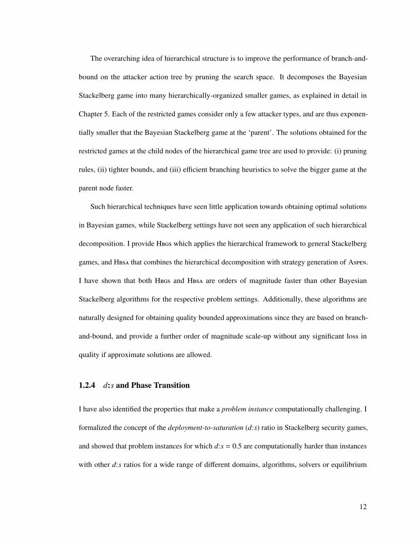
The overarching idea of hierarchical structure is to improve the performance of branch-and-

bound on the attacker action tree by pruning the search space. It decomposes the Bayesian

Stackelberg game into many hierarchically-organized smaller games, as explained in detail in

Chapter 5. Each of the restricted games consider only a few attacker types, and are thus exponen-

tially smaller that the Bayesian Stackelberg game at the ‘parent’. The solutions obtained for the

restricted games at the child nodes of the hierarchical game tree are used to provide: (i) pruning

rules, (ii) tighter bounds, and (iii) efficient branching heuristics to solve the bigger game at the

parent node faster.

Such hierarchical techniques have seen little application towards obtaining optimal solutions

in Bayesian games, while Stackelberg settings have not seen any application of such hierarchical

decomposition. I provide Hbgs which applies the hierarchical framework to general Stackelberg

games, and Hbsa that combines the hierarchical decomposition with strategy generation of Aspen.

I have shown that both Hbgs and Hbsa are orders of magnitude faster than other Bayesian

Stackelberg algorithms for the respective problem settings. Additionally, these algorithms are

naturally designed for obtaining quality bounded approximations since they are based on branch-

and-bound, and provide a further order of magnitude scale-up without any significant loss in

quality if approximate solutions are allowed.

1.2.4 d:s and Phase Transition

I have also identified the properties that make a problem instance computationally challenging. I

formalized the concept of the deployment-to-saturation (d:s) ratio in Stackelberg security games,

and showed that problem instances for which d:s = 0.5 are computationally harder than instances

with other d:s ratios for a wide range of different domains, algorithms, solvers or equilibrium

12

computation methods [Jain et al., 2012]. This work also provides evidence that the computationally

hard region is also one where optimization is most beneficial to the real-world security agencies,

thereby corroborating the need for algorithmic advances.

Furthermore, I use the concept of phase transitions to better understand this computationally

hard region. I define a decision problem related to security games, and show that the probability that

this problem has a solution exhibits a phase transition as the d : s ratio crosses 0.5. This provides

evidence that security games with d : s = 0.5 are indeed computationally more challenging.

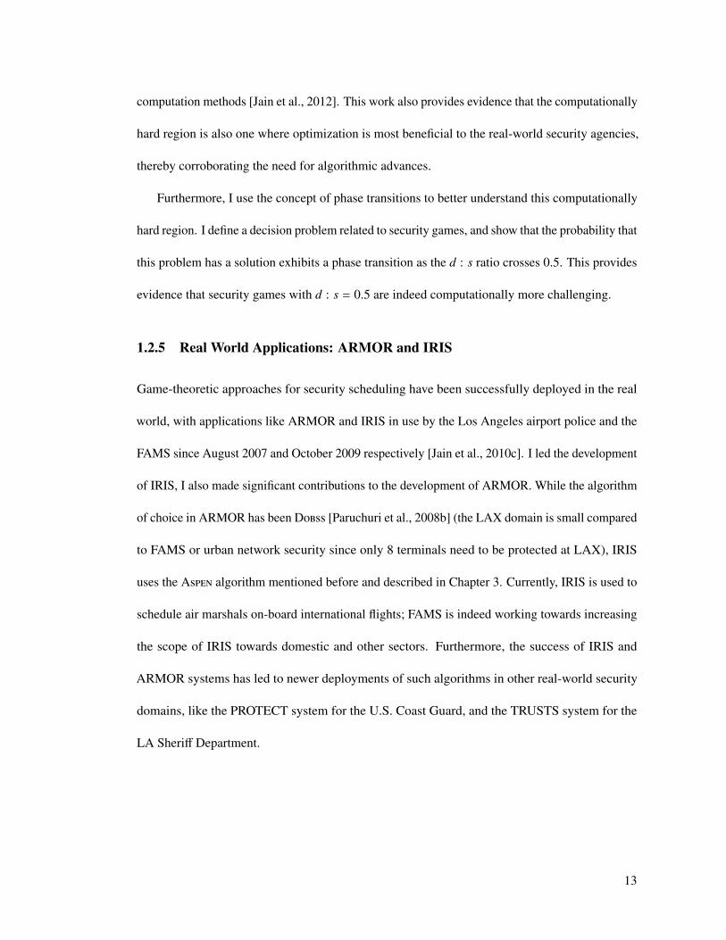
1.2.5 Real World Applications: ARMOR and IRIS

Game-theoretic approaches for security scheduling have been successfully deployed in the real

world, with applications like ARMOR and IRIS in use by the Los Angeles airport police and the

FAMS since August 2007 and October 2009 respectively [Jain et al., 2010c]. I led the development

of IRIS, I also made significant contributions to the development of ARMOR. While the algorithm

of choice in ARMOR has been Dobss [Paruchuri et al., 2008b] (the LAX domain is small compared

to FAMS or urban network security since only 8 terminals need to be protected at LAX), IRIS

uses the Aspen algorithm mentioned before and described in Chapter 3. Currently, IRIS is used to

schedule air marshals on-board international flights; FAMS is indeed working towards increasing

the scope of IRIS towards domestic and other sectors. Furthermore, the success of IRIS and

ARMOR systems has led to newer deployments of such algorithms in other real-world security

domains, like the PROTECT system for the U.S. Coast Guard, and the TRUSTS system for the

LA Sheriff Department.

13

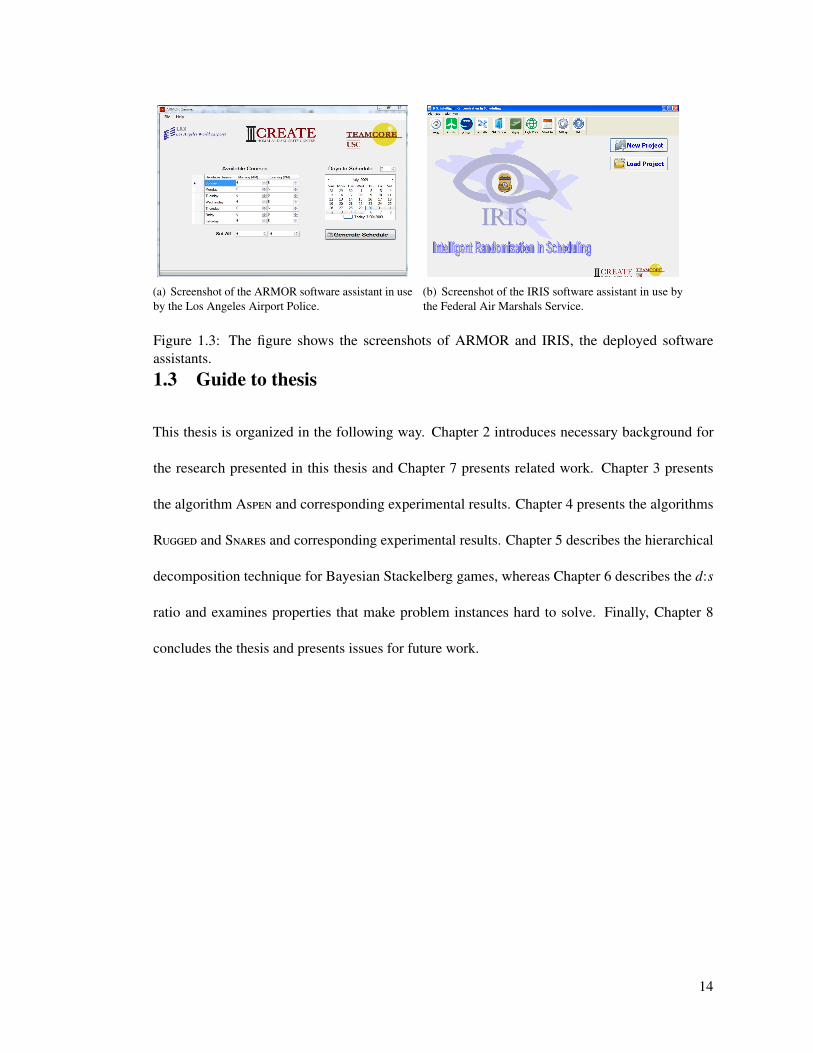
(a) Screenshot of the ARMOR software assistant in useby the Los Angeles Airport Police.

(b) Screenshot of the IRIS software assistant in use bythe Federal Air Marshals Service.

Figure 1.3: The figure shows the screenshots of ARMOR and IRIS, the deployed softwareassistants.

1.3 Guide to thesis

This thesis is organized in the following way. Chapter 2 introduces necessary background for

the research presented in this thesis and Chapter 7 presents related work. Chapter 3 presents

the algorithm Aspen and corresponding experimental results. Chapter 4 presents the algorithms

Rugged and Snares and corresponding experimental results. Chapter 5 describes the hierarchical

decomposition technique for Bayesian Stackelberg games, whereas Chapter 6 describes the d:s

ratio and examines properties that make problem instances hard to solve. Finally, Chapter 8

concludes the thesis and presents issues for future work.

14

Chapter 2: Background

This chapter begins by introducing motivating examples of real world security applications in

Section 2.1. The work in this thesis builds on Stackelberg games for modeling security domains,

and so I then provide the background on the general Stackelberg game model and its Bayesian

extension in Section 2.2. Section 2.3 introduces the standard solution concept known as the Strong

Stackelberg Equilibrium (SSE). Section 2.4 then talks about the security game representation for

Stackelberg games, whereas Section 2.5 describes security game models with arbitrary scheduling

constraints. Section 2.6 then introduces security game model with patrolling constraints, followed

by description of network security domains in Section 2.8. Finally, Section 2.9 overviews previous

algorithms of relevance to this thesis.

2.1 Motivating Domains

Security scenarios addressed in this work exhibit the following important characteristics: there is a

leader/follower dynamic between the security forces and terrorist adversaries, since the security

forces commit to a security policy first while the adversaries conduct surveillance to exploit any

weaknesses or patterns in the security strategies [Tambe, 2011]. A security policy here refers to

some schedule to patrol, check or monitor the area under protection. There are limited security

15

resources available to protect a very large space of possible targets, so it is not possible to provide

complete coverage at all times. Moreover, the targets in the real-world clearly have different

values and vulnerabilities in each domain. Additionally, there is uncertainty over many adversary

types. For example, the security forces may not know whether they would face a well-funded

terrorist or a local gang member or some other threat. Typically, the security forces are interested

in a randomized schedule, so that surveillance does not yield predictable patterns; yet they wish

to ensure that more important targets have a higher protection and that they guard against an

intelligent adversary’s adaptive response to their randomized schedule. I now describe some

concrete security domains which have motivated my research.

2.1.1 Los Angeles International Airport (LAX):

LAX is the fifth busiest airport in the United States, the largest destination airport in the United

States, and serves 60-70 million passengers per year [LAWA, 2007; Stevens and et. al., 2006].

The LAX police use diverse measures to protect the airport, which include vehicular checkpoints,

police units patrolling the roads to the terminals, patrolling inside the terminals (with canines), and

security screening and bag checks for passengers. The application of game-theoretic approach is

focused on two of these measures: (1) placing vehicle checkpoints on inbound roads that service

the LAX terminals, including both location and timing (2) scheduling patrols for bomb-sniffing

canine units at the different LAX terminals.

The eight different terminals at LAX have very different characteristics, like physical size,

passenger loads, foot traffic or international versus domestic flights. These factors contribute

to the differing risk assessments of these eight terminals. The numbers of available vehicle

checkpoints and canine units are limited by resource constraints, so the key challenge is to apply

16

game-theoretic algorithms to intelligently allocate these resources – typically in a randomized

fashion — to improve their effectiveness while avoiding patterns in the scheduled deployments.

2.1.2 United States Federal Air Marshals Service (FAMS):

The FAMS places undercover law enforcement personnel aboard flights of US air carriers origi-

nating in and departing the United States to dissuade potential aggressors and prevent an attack

should one occur [TSA, 2008]. The exact methods used to evaluate the risks posed by individual

flights is not made public by the service, and many factors might influence such an evaluation.

For example, flights have different numbers of passengers, and some fly over densely populated

areas while others do not [TSA, 2008]. International flights also serve different countries, which

may pose different risks. Special events can also change the risks for particular flights at certain

times [Wiki, 2008]. The scale of the domain is massive. There are currently tens of thousands

of commercial flights scheduled each day, and public estimates state that there are thousands of

air marshals [CNN, 2008]. Air marshals must be scheduled on tours of flights that obey various

constraints (e.g., the time required to board, fly, and disembark). Simply finding schedules for the

marshals that meet all of these constraints is a computational challenge. The task is made more

difficult by the need to find a randomized policy that meets these scheduling constraints, while

also accounting for the different values of each flight.

2.1.3 United States Transportation Security Agency (TSA):

The TSA is tasked with protecting the nation’s transportation systems [TSA, 2011a]. One set

of systems in particular is the over 400 airports [TSA, 2011a] which services approximately

28,000 commercial flights and up to approximately 87,000 total flights [ATC, 2011] per day. To

17

protect this large transportation network, the TSA employs approximately 48,000 Transportation

Security Officers [TSA, 2011a], who are responsible for implementing security activities at each

individual airport. While many people are aware of common security activities, such as individual

passenger screening, this is just one of many security layers TSA personnel implement to help

prevent potential threats [TSA, 2011b,a]. These layers can involve hundreds of heterogeneous

security activities executed by limited TSA personnel leading to a complex resource allocation

challenge. While activities like passenger screening are performed for every passenger, the TSA

cannot possibly run every security activity all the time. Thus, while the resources required for

passenger screening are always allocated by the TSA, it must also decide how to appropriately

allocate its remaining security officers among the layers of security to protect against a number

of potential threats, while facing challenges such as surveillance and an adaptive adversary as

mentioned before.

2.1.4 United States Coast Guard:

The US Coast Guard patrols harbors to safeguard the maritime and security interests of the country.

The Coast Guard continues to face a challenging future with an evolving asymmetric threat within

the maritime environment both within the Maritime Global Commons but also within the ports

and waterways that make up the United States Maritime Transportation System (MTS). The Coast

Guard can cover any subset of patrol areas in any patrol schedule. They can also perform many

security activities at each patrol area. The challenge for the Coast Guard again is to design a

randomized patrolling strategy given that they need to protect a diverse set of targets along the

harbor and the attacker conducts surveillance and is adaptive.

18

2.2 Stackelberg Games

In a Stackelberg game, a leader commits to a strategy first, and then followers sequentially selfishly

optimize their rewards, considering the action chosen by the leader. For the remainder of this

thesis, I will refer to the leader as ‘her’ and the follower as ‘him’. To see the advantage of being the

leader in a Stackelberg game, consider a simple game with the payoff table as shown in Table 2.1,

which was first presented by [Conitzer and Sandholm, 2006]. The leader is the row player and the

follower is the column player. The only pure-strategy Nash equilibrium for this game is when the

leader plays a and the follower plays c, which gives the leader a payoff of 2; in fact, for the leader,

playing b is strictly dominated. However, if the leader can commit to playing b before the follower

chooses his strategy, then the leader will obtain a payoff of 3, since the follower would then play d

to ensure a higher payoff for himself. If the leader commits to a uniform mixed strategy of playing

a and b with equal (0.5) probability, then the follower will play d, leading to a payoff for the leader

of 3.5.

Target 1 Target 2Target 1 2, 1 4, 0Target 2 1, 0 3, 2

Table 2.1: Payoff table for example Stackelberg game.

The Stackelberg games I consider in this thesis have two agents, the leader (defender), Θ, and

the follower (attacker/adversary), Ψ. Each player has a set of possible pure strategies, denoted

σΘ ∈ ΣΘ and σΨ ∈ ΣΨ. A mixed strategy allows a player to play a probability distribution over

pure strategies, denoted x and a for the leader and the follower respectively. Payoffs for each

player are defined over all possible joint pure-strategy outcomes: UΘ : ΣΘ × ΣΨ → R for the

defender and similarly for each attacker. The payoff functions are extended to mixed strategies in

19

the standard way by taking the expectation over pure-strategy outcomes. The follower can observe

the leader’s strategy, and then act in a way to optimize its own payoffs. Formally, the attacker’s

strategy in a Stackelberg security game becomes a function that selects a strategy for each possible

leader strategy: FΨ : x→ a.

The Bayesian extension to Stackelberg games allows for each player (leader or follower) to be

one of multiple possible types, with each type associated with its own payoff values. In this thesis,

the defender (leader), Θ, only has one type since she is considering her own personal resources.

However, the attacker (follower) can be one of a set of possible types denoted by λ ∈ Λ. For

example, a security force may be interested in protecting against potential terrorist attacks and

catching potential drug smugglers, which represent two different types of adversaries. Each type is

represented by a different and possibly uncorrelated payoff matrix for both the leader and follower.

That is, the leader’s payoffs will vary along with the follower’s payoffs for each type of follower.

At any time the leader does not know what follower type she will face, however, she is aware

of the probability distribution over follower types (i.e., she knows how frequently she will face

each follower type). The probability with which follower type λ ∈ Λ appears is denoted by pλ.

The follower is always aware of his own type and thus always has perfect information about the

leader’s payoffs and his own payoffs. The notation used in this thesis when referring to Bayesian

Stackelberg games is given in Table 2.2.

Given this formal model, the leader’s goal is to determine the mixed strategy x, such that

her expected value is maximized given that each follower type will choose his expected-value-

maximizing action with complete knowledge of the leader’s mixed strategy. Such a commitment

20

Variable DefinitionΘ Refers to the leaderΨ Refers to the followerΛ Set of follower typesΣΘ Set of pure strategies of the leaderΣΨ Set of pure strategies of the followerpλ Probability of follower type λ

G(Θ,ΨΛ) Bayesian Stackelberg gameUΘ Payoffs for the leaderUΨ Payoffs for the followerx Leader’s strategya Follower’s strategy

Table 2.2: Notation

to a mixed strategy models a real-world situation where security forces commit to a randomized

patrolling strategy first. Given this commitment, an adversary can conduct as much surveillance of

this mixed strategy as he desires. Even with knowledge of this mixed strategy, the adversary has

no specific knowledge of what the security force may do on a particular day however. He only

has knowledge of the mixed strategy the security force will use to decide her resource allocations

for that day. In this model, predictable defense strategies are vulnerable to exploitation by a

determined adversary.

2.3 Strong Stackelberg Equilibrium (SSE)

The most common solution concept in game theory is a Nash equilibrium, which is a profile of

strategies for each player in which no player can gain by unilaterally changing to another strategy

[Osbourne and Rubinstein, 1994]. Stackelberg equilibrium is a refinement of Nash equilibrium

specific to Stackelberg games. It is a form of sub-game perfect equilibrium in that it requires

that each player select the best-response in any subgame of the original game (where subgames

correspond to partial sequences of actions). The effect is to eliminate equilibrium profiles that

21

are supported by non-credible threats off the equilibrium path. Subgame perfection is a natural

requirement, but it does not guarantee a unique solution in cases where the follower is indifferent

among a set of strategies. The literature contains two form of Stackelberg equilibria that identify

unique outcomes, first proposed by Leitmann [Leitmann, 1978], and typically called “strong” and

“weak” after Breton et. al. [Breton et al., 1988]. The strong form assumes that the follower will

always choose the optimal strategy for the leader in cases of indifference, while the weak form

assumes that the follower will choose the worst strategy for the leader. Unlike the weak form,

strong Stackelberg equilibria are known to exist in all Stackelberg games [Basar and Olsder, 1995].

A standard argument suggests that the leader is often able to induce the favorable strong form by

selecting a strategy arbitrarily close to the equilibrium which causes the follower to strictly prefer

the desired strategy [von Stengel and Zamir, 2004]. We adopt strong Stackelberg equilibrium as

our solution concept in part for these reasons, but also because it is the most commonly used in

related literature [Osbourne and Rubinstein, 1994; Conitzer and Sandholm, 2006; Paruchuri et al.,

2008b].

Definition 1. A set of strategies (δΘ, FΨ) form a Strong Stackelberg Equilibrium (SSE) if they

satisfy the following:

1. The leader plays a best-response:

UΘ(x, FΨ(x)) ≥ UΘ(x′, FΨ(x′)) ∀ x′.

2. The follower plays a best-response:

UΨ(x, FΨ(x)) ≥ UΨ(x, a) ∀ a.

22

3. The follower breaks ties optimally for the leader:

UΘ(x, FΨ(x)) ≥ UΘ(x, a) ∀ x, a ∈ Σ∗Ψ

(x), where Σ∗Ψ

(x) is the set of follower best-responses,

as above.

In the case of Bayesian games with many follower types Λ, the leader’s best response is a

weighted best response to the followers’ responses, where the weights are based on the probability

of occurrence of each type (pλ). The strategy of each attacker type γ becomes: FγΨ

, which still

satisfies constraints 2 and 3 in Definition 1.

2.4 Stackelberg Security Games

In a security game, a defender must perpetually defend the site in question, whereas the attacker is

able to observe the defender’s strategy and attack when success seems most likely. This fits neatly

into the description of a Stackelberg game if we map the attackers to the follower’s role and the

defender to the leader’s role [Avenhaus et al., 2002; Brown et al., 2006; Kiekintveld et al., 2009].

The actions for the security forces represent the action of scheduling a patrol or checkpoint, e.g. a

checkpoint at the LAX airport or a federal air marshal scheduled to a flight. The actions for an

adversary represent an attack at the corresponding infrastructural entity. The strategy for the leader

is a mixed strategy spanning the various possible actions.

There are two major problems with using conventional methods to represent security games in

normal form. First, many solution methods require the use of a Harsanyi transformation when

dealing with Bayesian games [Harsanyi and Selten, 1972]. The Harsanyi transformation converts

a Bayesian game into a normal-form game, but the new game may be exponentially larger than

the original Bayesian game. The compact representation of security games avoids this Harsanyi

23

transformation, and instead directly operates on the Bayesian game. Operating directly on the

Bayesian representation is possible in security games because the evaluation of the leader strategy

against a Harsanyi-transformed game matrix is equivalent to its evaluation against each of the game

matrices for the individual follower types [Kiekintveld et al., 2009]. The second problem arises

that the defender has many possible resources to schedule in the security policy. This can also lead

to a combinatorial explosion in a standard normal-form representation. For example, if the leader

has m resources to defend n entities, then normal-form representations model this problem as a

single leader with(

nm

)rows, each row corresponding to a leader action of covering m targets with

security resources. However, in the security game representation, the game representation would

only include n rows, each row corresponding to whether the corresponding target was covered

or not. Such a representation is equivalent to the normal form representation if the defender

does not face any scheduling constraints (examples of domains with scheduling constraints will

be given in Sections 2.5 to 2.8 – for the same reason, such problems are also referred to as

Security Problems with No Scheduling Constraints (SPNSC) in this thesis). This compactness

in SPNSC is possible because the payoffs for the leader in these games simply depend on whether

the attacked target was covered or not, and not on what other targets were covered (or not covered).

The representation we use here avoids both of these potential problems, using methods similar

to other compact representations for games [Koller and Milch, 2003; Jiang and Leyton-Brown,

2006].

I now introduce this compact representation for security games. Let T = {t1, . . . , tn} be a set

of targets that may be attacked, corresponding to pure strategies for the attacker. The defender

has a set of resources available to cover these targets, R = {r1, . . . , rm} (for example, in the FAMS

domain, targets could be flights and resources could be federal air marshals). Associated with

24

each target are four payoffs defining the possible outcomes for an attack on the target, as shown

in Table 2.3. Similarly, 2.4 shows an example for an entire Bayesian security game with no

scheduling constraints with two targets. There are two cases, depending on whether or not the

target is covered by the defender. The defender’s payoff for an uncovered attack when facing an

adversary of type γ is denoted Uγ,uΘ

(t), and for a covered attack Uγ,cΘ

(t). Similarly, Uγ,uΨ

(t) and

Uγ,cΨ

(t) are the payoffs of the attacker.

Covered UncoveredDefender 5 –20Attacker –10 30

Table 2.3: Example payoffs for an attack on a target.

Attacker Type 1Defender Attacker

Target Cov. Uncov. Cov. Uncov.t1 10 0 -1 1t2 0 -10 -1 1

Attacker Type 2Defender Attacker

Target Cov. Uncov. Cov. Uncov.t1 5 -4 -2 1t2 4 -5 -1 2

Table 2.4: Example Bayesian security game with two targets and two attacker types.

A crucial feature of the model is that payoffs depend only on the target attacked, and whether

or not it is covered by the defender. The payoffs do not depend on the remaining aspects of the

schedule, such as whether any unattacked target is covered or which specific defense resource

provides coverage. For example, if an adversary succeeds in attacking Terminal 1, the penalty for

the defender is the same whether the defender was guarding Terminal 2 or 3. Therefore, from

a payoff perspective, many resource allocations by the defender are identical. We exploit this

by summarizing the payoff-relevant aspects of the defender’s strategy in a coverage vector, C,

that gives the probability that each target is covered, ct. The analogous attack vector Aγ gives the

25

probability of attacking a target by a follower of type γ. We restrict the attack vector for each

follower type to attack a single target with probability 1. This is without loss of generality because

a strong Stackelberg equilibrium (SSE) solution still exists under this restriction [Paruchuri et al.,

2008b]. Thus, the follower of type γ can choose any pure strategy σγΨ∈ Σ

γΨ

, that is, attack any one

target from the set of targets.

The payoff for a defender when a specific target t is attacked by an adversary of type γ is

given by UγΘ

(t,C) and is defined in Equation 2.1. Thus, the expectation of UγΘ

(t,C) over t gives

UγΘ

, which is the defender’s expected payoff given coverage vector C when facing an adversary

of type γ whose attack vector is Aγ. UγΘ

is defined in Equation 2.2. The same notation applies

for each follower type, replacing Θ with Ψ. Thus, UγΨ

(t,C) gives the payoff to the attacker when

a target t is attacked by an adversary of type γ. We also define the useful notion of the attack

set in Equation 2.3, Λγ(C), which contains all targets that yield the maximum expected payoff

for the attacker type γ given coverage C. This attack set is used by the adversary to break ties

when calculating a strong Stackelberg equilibrium. Moreover, in these security games, exactly one

adversary is attacking in one instance of the game; however, the adversary could be of any type

and the defender does not know the type of the adversary faced.

UγΘ

(t,C) = ctUγ,cΘ

(t) + (1 − ct)Uγ,uΘ

(t) (2.1)

UγΘ

(C, Aγ) =∑t∈T

aγt · (ct · Uγ,cΘ

(t) + (1 − ct)Uγ,uΘ

(t)) (2.2)

Λγ(C) = {t : UγΨ

(t,C) ≥ UγΨ

(t′,C) ∀ t′ ∈ T }. (2.3)

26

In a strong Stackelberg equilibrium, the attacker selects the target in the attack set with maximum

payoff for the defender. Let t∗ denote this optimal target. Then the expected SSE payoff for the

defender when facing this adversary of type γ with probability pγ is UγΘ

(C) = UγΘ

(t∗,C) × pγ, and

for the attacker UγΨ

(C) = UγΨ

(t∗,C).

2.5 Security Problems with Arbitrary Scheduling Constraints

(SPARS)

I now introduce the SPARS domain, which includes arbitrary scheduling constraints for the

defender. A SPARS game is a security game where each defender resource can be assigned to a

schedule covering multiple targets, s ⊆ T , so the set of all legal schedules is defined as S ⊆ P(T ).

The defender has R resources, such that each defender resource r is restricted to a set of legal

schedules, S r ⊆ S (note that this implies that defender resources are no longer identical). The

defender’s pure strategies are the set of joint schedules that assign each resource to at most one

schedule. Additionally, we assume that a target may be covered by at most 1 resource in a joint

schedule (though this can be generalized). A joint schedule j can be represented by the vector

Pj = 〈P jt〉 ∈ {0, 1}n where P jt represents whether or not target t is covered in joint schedule j.

The set of all feasible joint schedules is denoted by J. We define a mapping M from j to Pj as:

M(j) = 〈P jt〉, where P jt = 1 if t ∈⋃

s∈j s; 0 otherwise. The defender’s mixed strategy x specifies

the probabilities of playing each j ∈ J, where each individual probability is denoted by x j. Let

c = 〈ct〉 be the vector of coverage probabilities corresponding to x, where ct =∑

j∈J P jt x j is the

marginal probability of covering t.

27

A Bayesian-SPARS instance is an extension for the SPARS problem for many attacker types.

Thus, each target in Bayesian-SPARS now has many sets of payoffs, one for each attacker type.

For reference, Table 2.5 summarizes all of the notation introduced here, and builds on the notation

presented in Table 2.2 for SPNSC problems.

Example: Consider a FAMS game with 5 targets (flights), T = {t1, . . . , t5}, and three marshals

of the same type, R = 3, S 1 = S 2 = S 3 = S . Let the set of feasible schedules be S =

{{t1, t2}, {t2, t3}, {t3, t4}, {t4, t5}, {t1, t5}}. The set of feasible joint schedules is shown below, where

column j1 represents the joint schedule {{t1, t2}, {t3, t4}}.

P =

j1 j2 j3 j4 j5

t1 :

t2 :

t3 :

t4 :

t5 :

1 1 1 1 0

1 1 1 0 1

1 1 0 1 1

1 0 1 1 1

0 1 1 1 1

Each joint schedule in J assigns only 2 air marshals in this example, since no more than 1 air

marshal is allowed on any flight. Thus, the third air marshal will remain unused. Suppose all

of the targets have identical payoffs UcΘ

(t) = 1, UuΘ

(t) = −5, UcΨ

(t) = −1 and UuΨ

(t) = 5. In

this case, the optimal strategy for the defender randomizes uniformly across the joint schedules,

x = 〈.2, .2, .2, .2, .2〉, resulting in coverage c = 〈.8, .8, .8, .8, .8〉. All pure strategies have equal

28

payoffs for the attacker, given this coverage vector. Furthermore, for this example, ERASER-C

incorrectly outputs the coverage vector c = 〈1, 1, 1, 1, 1〉.1

To summarize, a solution to the SPARS problem instance is the optimal mixed strategy over

joint schedules, such that each joint schedule assigns every defender resource to a schedule (or

a set of targets). This mixed strategy is indexed over joint schedules, where the number of joint

schedules is combinatorial in the number of schedules S and the number of defender resources.

In Chapter 3, I introduce the Aspen algorithm that uses branch-and-price to compute solutions to

SPARS instances with just one attacker type (non-Bayesian). This algorithm is extended to handle

the Bayesian case in Chapter 5.

2.6 Security Problems with Patrolling Constraints (SPPC)

I now introduce a new domain: Security Problems with Patrolling Constraints (SPPC). This is

a generalized security domain that allows us to consider many different facets of the patrolling

problem. The defender needs to protect a set of targets, located geographically on a plane, using a

limited number of resources. These resources start at a given target and then conduct a tour that

can cover an arbitrary number of additional targets; the constraint is that the total tour length must

not exceed a given parameter L. I consider two variants of this domain featuring different attacker

models.1This coverage vector is incorrect since there does not exist a mixed strategy over joint schedules for the defender

that can achieve these marginals.

29

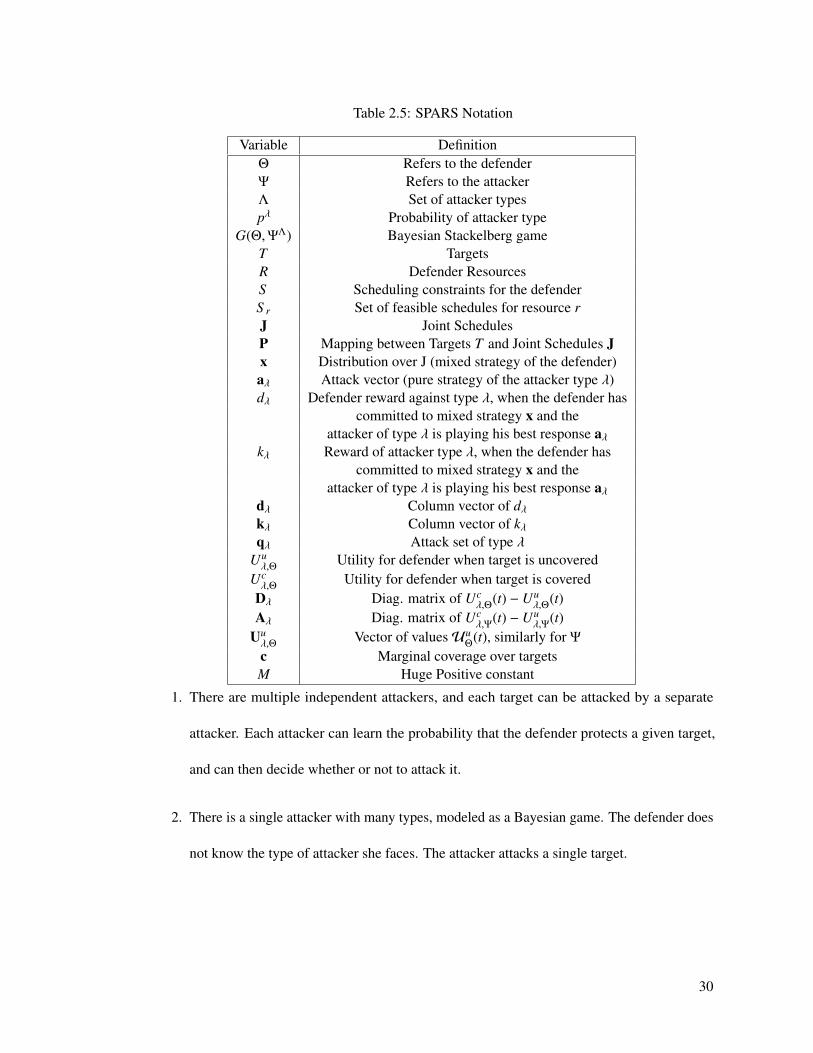
Table 2.5: SPARS Notation

Variable DefinitionΘ Refers to the defenderΨ Refers to the attackerΛ Set of attacker typespλ Probability of attacker type

G(Θ,ΨΛ) Bayesian Stackelberg gameT TargetsR Defender ResourcesS Scheduling constraints for the defenderS r Set of feasible schedules for resource rJ Joint SchedulesP Mapping between Targets T and Joint Schedules Jx Distribution over J (mixed strategy of the defender)aλ Attack vector (pure strategy of the attacker type λ)dλ Defender reward against type λ, when the defender has

committed to mixed strategy x and theattacker of type λ is playing his best response aλ

kλ Reward of attacker type λ, when the defender hascommitted to mixed strategy x and the

attacker of type λ is playing his best response aλdλ Column vector of dλkλ Column vector of kλqλ Attack set of type λ

Uuλ,Θ Utility for defender when target is uncovered

Ucλ,Θ Utility for defender when target is covered

Dλ Diag. matrix of Ucλ,Θ(t) − Uu

λ,Θ(t)Aλ Diag. matrix of Uc

λ,Ψ(t) − Uuλ,Ψ(t)

Uuλ,Θ Vector of valuesUu

Θ(t), similarly for Ψ

c Marginal coverage over targetsM Huge Positive constant

1. There are multiple independent attackers, and each target can be attacked by a separate

attacker. Each attacker can learn the probability that the defender protects a given target,

and can then decide whether or not to attack it.

2. There is a single attacker with many types, modeled as a Bayesian game. The defender does

not know the type of attacker she faces. The attacker attacks a single target.

30

Variable DefinitionS Set of sites (targets)T Set of toursL Upper bound on the length of a defender tourx Probability distribution over Tq Attack vectorzst Binary value indicating whether or not s ∈ Td Defender rewardk Adversary rewardP Penalty to attackerRs Reward to attacker at site sτs Defender reward for catching attacker on site sM Huge Positive constant

Table 2.6: Notation for the SPPC Domain

These variants were designed to capture properties of patrolling problems studied by researchers

across many real-world domains [An et al., 2011; Bosansky et al., 2011; Vanek et al., 2011]. An

example for the Bayesian single attacker setting is the US Coast Guard patrolling a set of targets

along the port to protect against potential threats. The defender’s objective is to find the optimal

mixed strategy x over tours T for all its resources in order to maximize her expected utility d. The

notation used for this domain is described in Table 2.6.

2.6.1 Payoff Structure

With each target in the domain are associated payoffs, which specify the payoff to both the defender

and the attacker in case of an successful or an unsuccessful attack. The attacker pays a high penalty

for getting caught, where as the defender gets a reward for catching the attacker. On the other hand,

if the attacker succeeds, the attacker gets a reward where as the defender pays a penalty. Both the

players get a payoff of 0 if the attacker chooses not to attack. The payoff matrix for each target

is given in Table 2.7. Thus, the defender gets a reward of τs units if she succeeds in protecting

31

the attack on target s, i.e. if the defender is covering the target s when it is attacked. On the other

hand, the attacker pays a penalty of −P on being caught. Similarly, the reward to the attacker is Rs

for a successful attack on site s, whereas the corresponding penalty to the defender for leaving the

target uncovered is −Rs.

No Attack AttackCovered 0, 0 τs,−P

Uncovered 0, 0 −Rs,Rs

Table 2.7: Payoff structure for each target: defender gets a reward of τs units for successfullypreventing an attack, while the attackers pays a penalty −P. Similarly, on a successful attack, theattacker gains Rs and the defender loses −Rs. Both players get 0 in case there is no attack.

2.7 Game Model 1: Multiple Attackers

In this game model, there are as many attackers as the number of targets in the domain. Each

attacker can choose to attack or not attack a distinct target. Each attacker can observe the net

coverage, or probability of the target being on a defender’s patrol, for the target that the attacker

is interested in. In our formulation, we assume that the attackers are independent and do not

coordinate or compete. Figure 2.1 shows an example problem and solutions for this example.

There are just two targets, A and B, which are placed 5 units away from the home (starting)

location of the defender’s resources. There are two attackers, one for each target. The tour length

allowed in this example was 10 units, that is, the defender can only patrol exactly one target in

each patrol route. The penalty P was set to 70 units where as the reward R for a successful attack

to the attacker was 100 units. For this particular example, the defender cannot protect the attacks

32

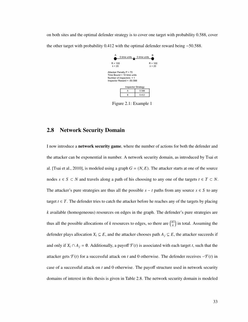
on both sites and the optimal defender strategy is to cover one target with probability 0.588, cover

the other target with probability 0.412 with the optimal defender reward being −50.588.

5 time units 5 time units

Attacker Penalty P = 70 Time Bound = 10 time units Number of inspectors = 1 Inspector Reward = -50.588

R = 100 λ = 20

R = 100 λ = 20

A   0.588  

B   0.412  

A B

Inspector Strategy

Figure 2.1: Example 1

2.8 Network Security Domain

I now introduce a network security game, where the number of actions for both the defender and

the attacker can be exponential in number. A network security domain, as introduced by Tsai et

al. [Tsai et al., 2010], is modeled using a graph G = (N, E). The attacker starts at one of the source

nodes s ∈ S ⊂ N and travels along a path of his choosing to any one of the targets t ∈ T ⊂ N.

The attacker’s pure strategies are thus all the possible s − t paths from any source s ∈ S to any

target t ∈ T . The defender tries to catch the attacker before he reaches any of the targets by placing

k available (homogeneous) resources on edges in the graph. The defender’s pure strategies are

thus all the possible allocations of k resources to edges, so there are(|E|k

)in total. Assuming the

defender plays allocation Xi ⊆ E, and the attacker chooses path A j ⊆ E, the attacker succeeds if

and only if Xi ∩ A j = ∅. Additionally, a payoff T (t) is associated with each target t, such that the

attacker gets T (t) for a successful attack on t and 0 otherwise. The defender receives −T (t) in

case of a successful attack on t and 0 otherwise. The payoff structure used in network security

domains of interest in this thesis is given in Table 2.8. The network security domain is modeled

33

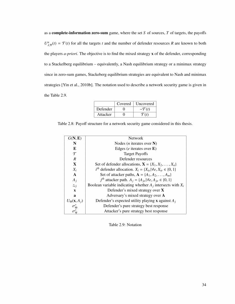
as a complete-information zero-sum game, where the set S of sources, T of targets, the payoffs

Uuλ,Ψ(t) = T (t) for all the targets t and the number of defender resources R are known to both

the players a-priori. The objective is to find the mixed strategy x of the defender, corresponding

to a Stackelberg equilibrium – equivalently, a Nash equilibrium strategy or a minimax strategy

since in zero-sum games, Stackeberg equilibrium strategies are equivalent to Nash and minimax

strategies [Yin et al., 2010b]. The notation used to describe a network security game is given in

the Table 2.9.

Covered UncoveredDefender 0 −T (t)Attacker 0 T (t)

Table 2.8: Payoff structure for a network security game considered in this thesis.

G(N,E) NetworkN Nodes (n iterates over N)E Edges (e iterates over E)T Target PayoffsR Defender resourcesX Set of defender allocations, X = {X1, X2, . . . , Xn}

Xi ith defender allocation. Xi = {Xie}∀e, Xie ∈ {0, 1}A Set of attacker paths, A = {A1, A2, . . . , Am}

A j jth attacker path. A j = {A je}∀e, A je ∈ {0, 1}zi j Boolean variable indicating whether A j intersects with Xi

x Defender’s mixed strategy over Xa Adversary’s mixed strategy over A

UΘ(x, A j) Defender’s expected utility playing x against A j

σ∗Θ

Defender’s pure strategy best responseσ∗

ΨAttacker’s pure strategy best response

Table 2.9: Notation

34

2.9 Baseline Algorithms

There is previous work on computing solutions for Bayesian Stackelberg games. These approaches

have ranged from solving the normal form Stackelberg game, solving security games to solving

the network security games. In this section, I briefly describe (i) MultipleLPs [Conitzer and Sand-

holm, 2006]; and (ii) DOBSS [Paruchuri et al., 2008b] for solving generic Bayesian Stackelberg

games, (iii) ERASER [Kiekintveld et al., 2009] for Bayesian Security games (SPNSC); and (iv)

RANGER [Tsai et al., 2010] for solving network security games. These approaches either do

not scale or do not compute optimal solutions for the problems of interest in my thesis; how-

ever, I describe them here since they provide background for algorithm design and experimental

evaluation.

2.9.1 Multiple LPs approach

The leader’s strategy in the SSE is considered the optimal leader’s strategy as it maximizes the

leader’s expected utility assuming the follower best responds. This section explains the baseline

algorithms for finding the optimal leader’s strategy of a Bayesian Stackelberg game. As shown by

Conitzer and Sandholm Conitzer and Sandholm [2006], the problem of computing the optimal

leader’s strategy x is equivalent to finding a leader’s mixed strategy x and a follower’s pure

strategy response a = g(x) such that the three SSE conditions (refer Definition 1) are satisfied.

Mathematically x can be found by solving the following maximization problem:

(x∗, σ∗Ψ) = arg maxx,σ∗Ψ

{UΘ(x, σ∗Ψ)|UλΨ(x, σλ∗Ψ ) ≥ Uλ

Ψ(x, σλ′

Ψ ),∀σλ′

Ψ ∈ ΣλΨ}. (2.4)

35

Here, σ∗Ψ

is the pure strategy for the Bayesian follower, and consists of σ∗Ψ

= 〈σλ∗Ψ〉, i.e., pure

strategy best responses for each follower type. x∗ refers to the optimal mixed strategy of the leader.

Equation (2.4) suggests the multiple linear program (LP) approach for finding x∗ as given

in [Conitzer and Sandholm, 2006]. The idea is to enumerate all possible pure strategy responses of

the follower σλΨ, λ ∈ Λ, σλ

Ψ∈ Σλ

Ψ. Furthermore, for each σΨ = 〈σλ

Ψ〉, the optimal mixed strategy

of the leader is chosen such that σΨ is a best response of the follower, and can be found by solving

the following LP:2

maxx

UΘ(x, σΨ)

s.t. x ≥ 0

1Tx = 1

UλΨ

(x, σλΨ

) ≥ UλΨ

(x, σλ′Ψ

), ∀λ ∈ Λ,∀σλ′

Ψ∈ Σλ

′

Ψ

(2.5)

Some of the LPs may be infeasible but it can be shown that at least one LP will return a feasible

solution. The optimal leader’s strategy x∗ is then the optimal solution of the LP which has the

highest objective value (i.e., the leader’s expected utility) among all feasible LPs.

2.9.2 Dobss: Mixed Integer Linear Program

Since the followers of different types are mutually independent of each other, there can be at most∏λ |Σ

λΨ| possible combinations of follower best response actions over the follower types. The

multiple LPs approach will then have to solve∏

λ |ΣλΨ| LPs and therefore its runtime complexity

grows exponentially in the number of follower types. In fact, the problem of finding the optimal

2Note the formulation here is slightly different from and has fewer constraints in each LP than the original multipleLPs approach in [Conitzer and Sandholm, 2006] where a Bayesian game is transformed to a normal-form one usingHarsanyi transformation [Harsanyi and Selten, 1972].

36

strategy for the leader in a Bayesian Stackelberg game with multiple follower types is NP-

hard [Conitzer and Sandholm, 2006]. Nevertheless, researchers have continued to provide practical

improvements. Dobss is an efficient general Stackelberg solver [Paruchuri et al., 2008b] and is in

use for security scheduling at the Los Angeles International Airport in the ARMOR system [Pita

et al., 2008]. Dobss obtains a decomposition scheme by exploiting the property that follower types

are independent of each other and solves the entire problem as one mixed-integer linear program

(MILP):

maxx,d,k,a

∑λ pλdλ

s.t. 1Tx = 1, x ≥ 0∑|ΣλΨ|

j=1 aλj = 1, ∀λ

aλj ∈ {0, 1}, ∀λ,∀ j = 1..|ΣλΨ|

dλ ≤ UλΘ

(x, j) + (1 − aλj ) · M, ∀λ,∀ j

0 ≤ kλ − UλΨ

(x, j) ≤ (1 − aλj ) · M, ∀λ,∀ j

(2.6)

Dobss effectively reduces the problem of solving an exponential number of LPs to a compactly

represented MILP which can be solved much more efficiently via modern techniques in Operations

Research. The key idea of the DobssMILP is to represent the strategy of each follower type aλ as

a binary vector aλ = [σλΨ1, σ

λΨ2, . . .] where σλ

Ψ j is 1 if the follower type λ chooses pure strategy j

and 0 otherwise. Here, UλΘ

(x, j) is the expected utility for the leader when the leader is playing

mixed strategy x and the follower is playing its jth pure strategy, i.e., σλΨ j. Uλ

Ψ(x, j) is also defined

similarly for the follower. M is (conceptually) an infinitely large constant.

37

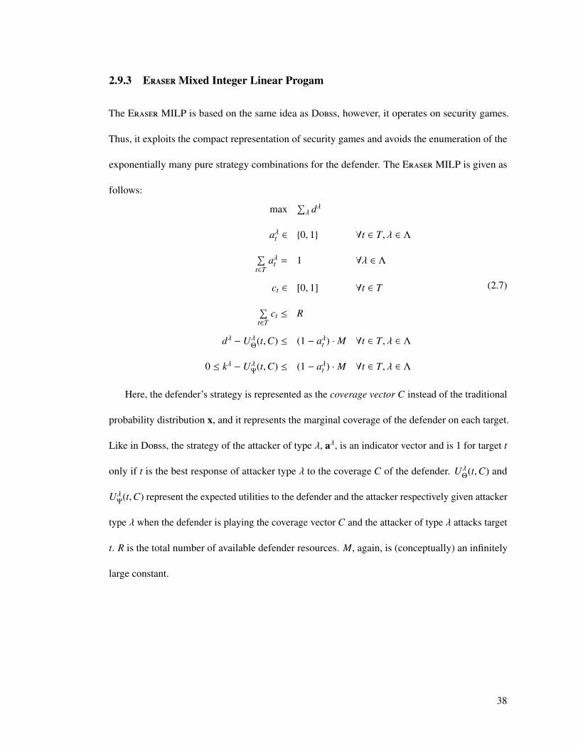
2.9.3 EraserMixed Integer Linear Progam

The Eraser MILP is based on the same idea as Dobss, however, it operates on security games.

Thus, it exploits the compact representation of security games and avoids the enumeration of the

exponentially many pure strategy combinations for the defender. The EraserMILP is given as

follows:

max∑λ dλ

aλt ∈ {0, 1} ∀t ∈ T, λ ∈ Λ∑t∈T

aλt = 1 ∀λ ∈ Λ

ct ∈ [0, 1] ∀t ∈ T∑t∈T

ct ≤ R

dλ − UλΘ

(t,C) ≤ (1 − aλt ) · M ∀t ∈ T, λ ∈ Λ

0 ≤ kλ − UλΨ

(t,C) ≤ (1 − aλt ) · M ∀t ∈ T, λ ∈ Λ

(2.7)

Here, the defender’s strategy is represented as the coverage vector C instead of the traditional

probability distribution x, and it represents the marginal coverage of the defender on each target.

Like in Dobss, the strategy of the attacker of type λ, aλ, is an indicator vector and is 1 for target t

only if t is the best response of attacker type λ to the coverage C of the defender. UλΘ

(t,C) and

UλΨ

(t,C) represent the expected utilities to the defender and the attacker respectively given attacker

type λ when the defender is playing the coverage vector C and the attacker of type λ attacks target

t. R is the total number of available defender resources. M, again, is (conceptually) an infinitely

large constant.

38

2.9.4 Ranger solution approach

Ranger [Tsai et al., 2010] provides approximate solutions to the network security game. It

approximates the strategy space of the players, using an efficient shortest-path based linear

program to perform the computation of the optimal defender allocation in the network. Tsai

et. al [Tsai et al., 2010] then provide two sampling schemes to sample from the mixed strategy

computed by Ranger to schedule the actual allocation of defender resources. The Ranger linear

program is given as follows:

max d∗

s.t. d∗ ≤ (1 − dt).T (t)

ds = 0

dv ≤ min(1, du + xe) ∀e = (u, v) ∈ E

0 ≤ xe ≤ 1 ∀e ∈ E∑e∈E xe ≤ R

(2.8)

In this Ranger linear program, d∗ is the defender reward computed by Ranger. xe is the marginal

probability of placing a checkpoint on edge e. The dv are, for each vertex v, the minimum sum

of checkpoint probabilities along any path from the source s to vertex v. The Ranger solution

overestimates the optimal defender reward, and as I show, in Chapter 4, the solution quality of

Ranger is unbounded.

39

Chapter 3: Strategy Generation for One Player

In this chapter, I show how strategy generation for one player can be used in domains where the

number of pure strategies for one player are extremely large. I will use two domains to demonstrate

the point: the SPARS domain as well as the SPPC domain. I will also show how strategy generation

can be used in conjunction with previously published algorithms to compute optimal defender

strategies in the SPARS domain. I conclude this section with experimental results in Section 3.4.

3.1 SPARS domain

In this section, I present Accelerated SPARS ENgine, Aspen, an algorithm that solves an instance

of the SPARS problem without having to enumerate all the pure strategies of the defender. Aspen

focuses on the non-Bayesian case (and so I omit the usage of the subscript λ in this section) –

I will describe the Bayesian extension in Chapter 5. Aspen formulates the SPARS problem as

a mixed-integer program in which the pure strategies of the attacker are represented by integer

variables a with at = 1 if target t is attacked and 0 otherwise. Two key computational challenges

arise in such a formulation. First, the space of possible strategies (joint schedules) for the defender

suffers from combinatorial explosion: a FAMS problem with 100 flights, schedules with 3 flights,

and 10 air marshals has up to 100,000 schedules and(100000

10

)joint schedules. Second, integer

40

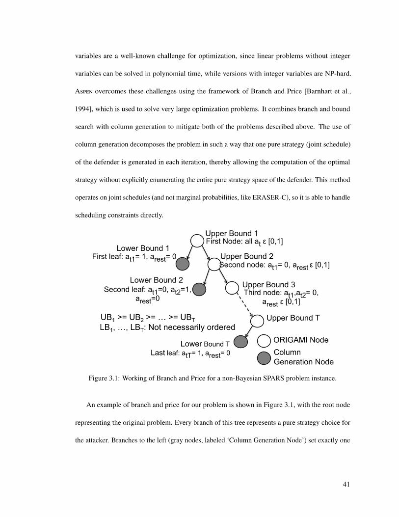
variables are a well-known challenge for optimization, since linear problems without integer

variables can be solved in polynomial time, while versions with integer variables are NP-hard.

Aspen overcomes these challenges using the framework of Branch and Price [Barnhart et al.,

1994], which is used to solve very large optimization problems. It combines branch and bound

search with column generation to mitigate both of the problems described above. The use of

column generation decomposes the problem in such a way that one pure strategy (joint schedule)

of the defender is generated in each iteration, thereby allowing the computation of the optimal

strategy without explicitly enumerating the entire pure strategy space of the defender. This method

operates on joint schedules (and not marginal probabilities, like ERASER-C), so it is able to handle

scheduling constraints directly.

First Node: all at ε [0,1]

First leaf: at1= 1, arest= 0 Second node: at1= 0, arest ε [0,1]

Second leaf: at1=0, at2=1, arest=0

Third node: at1,at2= 0, arest ε [0,1]

Last leaf: atT= 1, arest= 0

Upper Bound 1

UB1 >= UB2 >= … >= UBT LB1, …, LBT: Not necessarily ordered

Upper Bound 2

Upper Bound 3

Upper Bound T

Lower Bound 1

Lower Bound 2

Lower Bound T Column Generation Node

ORIGAMI Node

Figure 3.1: Working of Branch and Price for a non-Bayesian SPARS problem instance.

An example of branch and price for our problem is shown in Figure 3.1, with the root node

representing the original problem. Every branch of this tree represents a pure strategy choice for

the attacker. Branches to the left (gray nodes, labeled ‘Column Generation Node’) set exactly one

41

variable ti in a to 1 and the rest to zero, resulting in a linear program that gives a lower bound

on the overall solution quality. Branches to the right fix that same variable ti to zero, leaving the

remaining variables unconstrained. An upper bound on solution quality computed for each white

node (labeled as ‘ORIGAMI Node’) can be used to terminate execution without exploring all of

the possible integer assignments. This upper bound can be computed both naıvely as well as using

heuristics. In Section 3.1.2 we describe a heuristic based on the ORIGAMI algorithm that we use

in Aspen.

Solving the linear programs in each gray node normally requires enumerating all possible joint

schedules for the defender. Column generation (i.e., pricing) avoids this by iteratively solving a

restricted master problem, which includes only a small subset of the variables, and a slave problem

that identifies new variables to include in the master problem. The new variables added by the

slave problem are the ones that will maximally improve the objective value in the master problem.

The algorithm terminates when the slave problem cannot identify any new variables that will

improve the objective for the master problem.

Branch and price is not an “out of the box approach” and it has only recently begun to be

applied in game-theoretic settings [Halvorson et al., 2009a]. To apply the technique here, we

design a novel master-slave decomposition to facilitate column generation for SPARS, including a

network flow formulation of the slave problem. A standard technique for generating upper bounds

is to use a linear programming relaxation of the problem, but this approach performs poorly for

these problems based on our experimental results. Instead, we propose new methods for bounding

and selecting branches based on fast algorithms for security games without scheduling constraints.

42

3.1.1 ASPEN Column Generation

The linear programs at each leaf in Figure 3.1 are decomposed into master and slave problems

for column generation (see Algorithm 1). The master solves for the defender strategy x, given

a restricted set of columns (i.e., joint schedules) P, such that the attacker’s best response a is

consistent with the leaf node from Figure 3.1. The objective function for the slave is updated in

each iteration based on the current solution of the master problem. The slave problem is then

solved to identify the best new column to add to the master problem, using reduced costs (explained

later). If no column can improve the solution the algorithm terminates.

Algorithm 1 Column generation1. Initialize P2. Solve Master Problem3. Calculate reduced cost coefficients from solution4. Update objective of slave problem with coefficients5. Solve Slave Problemif Optimal solution obtained then

6. Return (x,P)else

7. Extract new column and add to P8. Repeat from Step 2

3.1.1.1 Master Problem:

The master problem (Equations 3.1 to 3.6) solves for the probability vector x that maximizes the

defender reward (Table 2.5 in the Chapter 2 succinctly lists the notation).1 This master problem

operates directly on columns of P, and the coverage vector c is computed from these columns

as Px. d represents the expected defender utility that is to be maximized, whereas d is a column

vector of d of dimension |T |. Similarly, k represents the attacker’s expected utility whereas k1The actual algorithm minimizes the negative of the defender reward for correctness of reduced cost computation

used in the Slave Problem; we show maximization of defender reward for expository purposes.

43

is a column vector of k of dimension |T |. The vectors d and k are introduced for dimensional

consistency in the matrix notation of the mixed integer linear program described below. While

the payoffs UuΘ

and UcΘ

for the defender are defined as before, D here is a diagonal matrix of

UcΘ

(t) − UuΘ

(t) of dimension |T | × |T |. Similarly, UuΨ

and UcΨ

represent the payoffs for the attacker

and A is a diagonal matrix of UcΨ

(t) − UuΨ

(t), again of dimension |T | × |T |.

Constraints 3.2–3.4 enforce the SSE conditions that the players choose mutual best responses.

Constraints 3.3 and 3.4 ensure that the assignment at = 1 can generate a feasible solution if

and only if target t is the best response of the attacker (note that this assignment is done when

resolving the branch of the branch-and-bound tree given in Figure 3.1). The defender expected

payoff (Equation 2.1) for target t is given by the tth component of the column vector DPx + UuΘ

and denoted (DPx + UuΘ

)t. Similarly, the attacker payoff for target t is given by (APx + UuΨ

)t.

Constraints 3.2 and 3.3 are active only for the single target t∗ attacked (at∗ = 1). This target must

be a best-response, due to Constraint 3.4. The pure strategy of the attacker a is an input to the

column generation procedure and not a variable for the formulation below.

max d (3.1)

s.t. d − DPx − UuΘ ≤ (1 − a)M (3.2)

k − APx − UuΨ ≤ (1 − a)M (3.3)

APx + UuΨ ≤ k (3.4)∑

j∈J

x j = 1 (3.5)

x ≥ 0 (3.6)

44

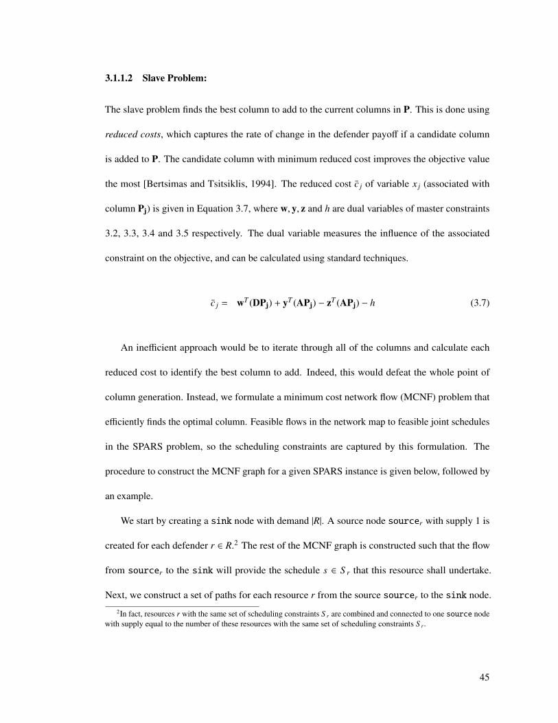
3.1.1.2 Slave Problem:

The slave problem finds the best column to add to the current columns in P. This is done using

reduced costs, which captures the rate of change in the defender payoff if a candidate column

is added to P. The candidate column with minimum reduced cost improves the objective value

the most [Bertsimas and Tsitsiklis, 1994]. The reduced cost c j of variable x j (associated with

column Pj) is given in Equation 3.7, where w, y, z and h are dual variables of master constraints

3.2, 3.3, 3.4 and 3.5 respectively. The dual variable measures the influence of the associated

constraint on the objective, and can be calculated using standard techniques.

c j = wT (DPj) + yT (APj) − zT (APj) − h (3.7)

An inefficient approach would be to iterate through all of the columns and calculate each

reduced cost to identify the best column to add. Indeed, this would defeat the whole point of

column generation. Instead, we formulate a minimum cost network flow (MCNF) problem that

efficiently finds the optimal column. Feasible flows in the network map to feasible joint schedules

in the SPARS problem, so the scheduling constraints are captured by this formulation. The

procedure to construct the MCNF graph for a given SPARS instance is given below, followed by

an example.

We start by creating a sink node with demand |R|. A source node sourcer with supply 1 is

created for each defender r ∈ R.2 The rest of the MCNF graph is constructed such that the flow

from sourcer to the sink will provide the schedule s ∈ S r that this resource shall undertake.

Next, we construct a set of paths for each resource r from the source sourcer to the sink node.

2In fact, resources r with the same set of scheduling constraints S r are combined and connected to one source nodewith supply equal to the number of these resources with the same set of scheduling constraints S r.

45

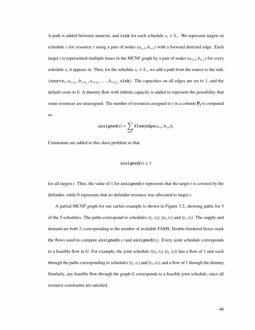
A path is added between sourcer and sink for each schedule sr ∈ S r. We represent targets in

schedule s for resource r using a pair of nodes (asr ,t, bsr ,t) with a forward directed edge. Each

target t is represented multiple times in the MCNF graph by a pair of nodes (asr ,t, bsr ,t) for every

schedule sr it appears in. Then, for the schedule sr ∈ S r, we add a path from the source to the sink:

〈sourcer, asr ,ti1 , bsr ,ti1 , asr ,ti2 , . . . , bsr ,tiL , sink〉. The capacities on all edges are set to 1, and the

default costs to 0. A dummy flow with infinite capacity is added to represent the possibility that

some resources are unassigned. The number of resources assigned to t in a column Pj is computed

as:

assigned(t) =∑s∈S

flow[edge(as,t, bs,t)].

Constraints are added to this slave problem so that

assigned(t) ≤ 1

for all targets t. Thus, the value of 1 for assigned(t) represents that the target t is covered by the

defender, while 0 represents that no defender resource was allocated to target t.

A partial MCNF graph for our earlier example is shown in Figure 3.2, showing paths for 3

of the 5 schedules. The paths correspond to schedules {t1, t2}, {t2, t3} and {t1, t5}. The supply and

demand are both 3, corresponding to the number of available FAMS. Double-bordered boxes mark

the flows used to compute assigned(t1) and assigned(t2). Every joint schedule corresponds

to a feasible flow in G. For example, the joint schedule {{t2, t3}, {t1, t5}} has a flow of 1 unit each

through the paths corresponding to schedules {t2, t3} and {t1, t5}, and a flow of 1 through the dummy.

Similarly, any feasible flow through the graph G corresponds to a feasible joint schedule, since all

resource constraints are satisfied.

46

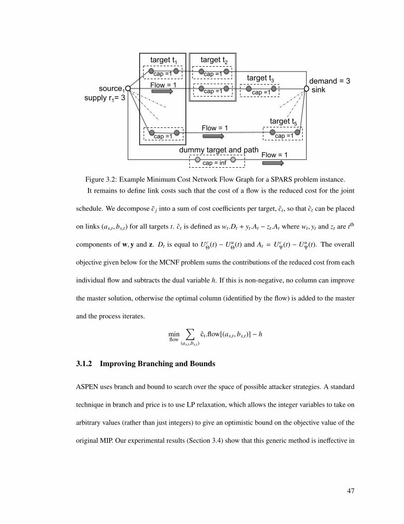
cap =1 cap =1

cap =1 cap =1

cap =1 cap =1

sink demand = 3

source1 supply r1= 3

target t1 target t2

target t3

dummy target and path cap = inf

target t5 Flow = 1

Flow = 1

Flow = 1

Figure 3.2: Example Minimum Cost Network Flow Graph for a SPARS problem instance.

It remains to define link costs such that the cost of a flow is the reduced cost for the joint

schedule. We decompose c j into a sum of cost coefficients per target, ct, so that ct can be placed

on links (as,t, bs,t) for all targets t. ct is defined as wt.Dt + yt.At − zt.At where wt, yt and zt are tth

components of w, y and z. Dt is equal to UcΘ

(t) − UuΘ

(t) and At = UcΨ

(t) − UuΨ

(t). The overall

objective given below for the MCNF problem sums the contributions of the reduced cost from each

individual flow and subtracts the dual variable h. If this is non-negative, no column can improve

the master solution, otherwise the optimal column (identified by the flow) is added to the master

and the process iterates.

minflow

∑(as,t ,bs,t)

ct.flow[(as,t, bs,t)] − h

3.1.2 Improving Branching and Bounds

ASPEN uses branch and bound to search over the space of possible attacker strategies. A standard

technique in branch and price is to use LP relaxation, which allows the integer variables to take on

arbitrary values (rather than just integers) to give an optimistic bound on the objective value of the

original MIP. Our experimental results (Section 3.4) show that this generic method is ineffective in

47

our domain. We introduce ORIGAMI-S, a novel branch and bound heuristic for SPARS based on

ORIGAMI [Kiekintveld et al., 2009], which is an efficient solution method for security games

without scheduling constraints and heterogeneous resources. We use ORIGAMI-S to solve a

relaxed version of SPARS that optimistically ignores scheduling constraints and integrate this with

ASPEN.

The ORIGAMI-S model is given in Equations 3.8–3.16. It minimizes the attacker’s maximum

payoff (Equations 3.8–3.10). The vector q represents the attack set, and is 1 for every target that

gives the attacker maximal expected payoff (Equation 3.10). The remaining non-trivial constraints

restrict the coverage probabilities. ORIGAMI-S defines a set of probabilities ct,s that represent the

coverage of each target t in each schedule s ∈ S r. The total coverage ct of target t is the sum of

coverage on t across individual schedules (Equation 3.11). We define a set Tr which contains one

target from each schedule s ∈ S r (e.g., choosing the first target from every schedule). The total

coverage assigned for every resource r is bounded from above by 1 (Equation 3.12), analogous to

the constraint that the total flow from the sourcer in the MCNF network flow graph cannot be

greater than the available supply of 1 resource.3 Total coverage is also bounded by multiplying the

number of resources by the maximum size of any schedule (L) in Equation 3.13. The defender can

3Again, as in the MCNF graph, resources with the same set of constraints S r are combined into one constraint, withthe available supply equal to the number of equivalent resources.

48

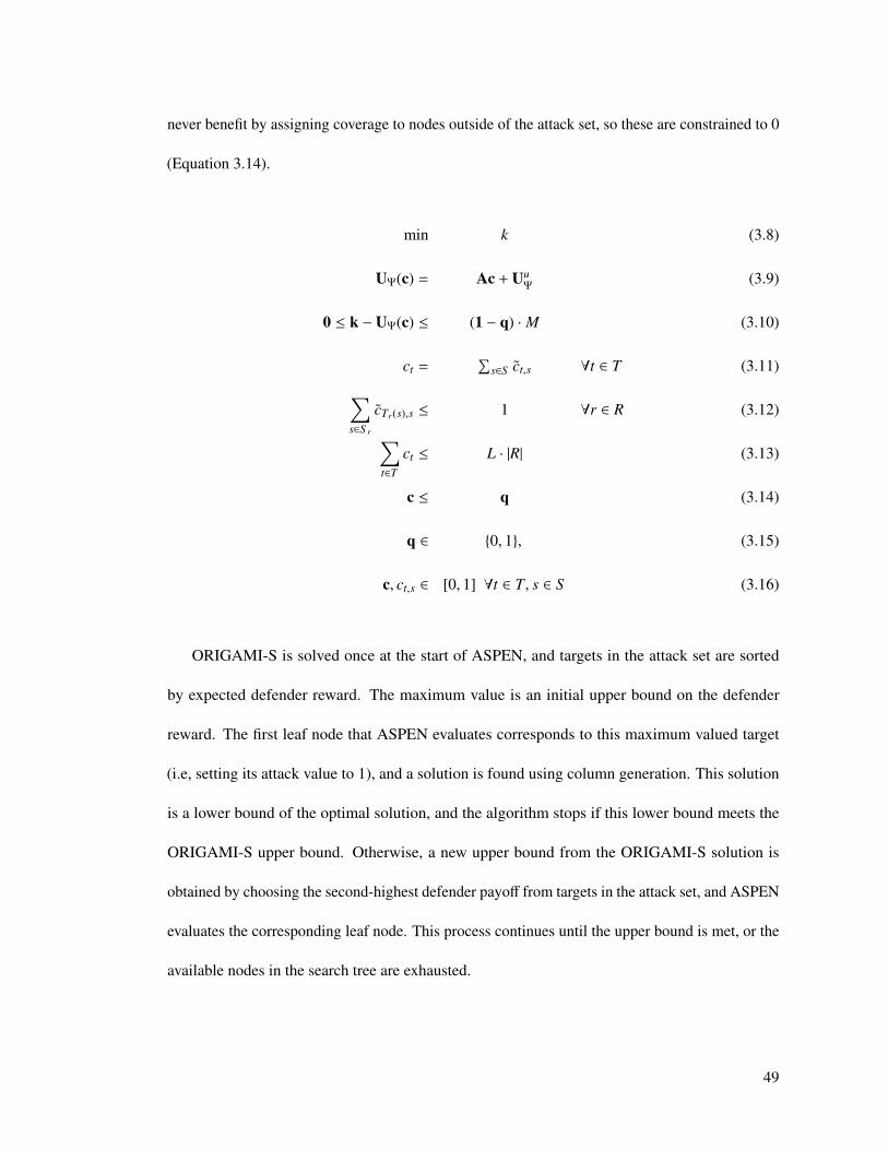
never benefit by assigning coverage to nodes outside of the attack set, so these are constrained to 0

(Equation 3.14).

min k (3.8)

UΨ(c) = Ac + UuΨ

(3.9)

0 ≤ k − UΨ(c) ≤ (1 − q) · M (3.10)

ct =∑

s∈S ct,s ∀t ∈ T (3.11)∑s∈S r

cTr(s),s ≤ 1 ∀r ∈ R (3.12)∑t∈T

ct ≤ L · |R| (3.13)

c ≤ q (3.14)

q ∈ {0, 1}, (3.15)

c, ct,s ∈ [0, 1] ∀t ∈ T, s ∈ S (3.16)

ORIGAMI-S is solved once at the start of ASPEN, and targets in the attack set are sorted

by expected defender reward. The maximum value is an initial upper bound on the defender

reward. The first leaf node that ASPEN evaluates corresponds to this maximum valued target

(i.e, setting its attack value to 1), and a solution is found using column generation. This solution

is a lower bound of the optimal solution, and the algorithm stops if this lower bound meets the

ORIGAMI-S upper bound. Otherwise, a new upper bound from the ORIGAMI-S solution is

obtained by choosing the second-highest defender payoff from targets in the attack set, and ASPEN

evaluates the corresponding leaf node. This process continues until the upper bound is met, or the

available nodes in the search tree are exhausted.

49

Theorem 1. The defender payoff, computed by ORIGAMI-S, is an upper bound on the defender’s

payoff for the corresponding SPARS problem. For any target not in the attack set of ORIGAMI-S,

the restricted SPARS problem in which this target is attacked is infeasible.

Proof Sketch: ORIGAMI and ORIGAMI-S both minimize the maximum attacker payoff over

a set of feasible coverage vectors. If there are no scheduling constraints, this also maximizes the

defender’s policy [Kiekintveld et al., 2009]. Briefly, the size of the attack set in the solution is

maximized, and the coverage probability on each target in the attack set is also maximal. Both of

these weakly improve the defender’s payoff because adding coverage to a target is strictly better

for the defender and worse for the adversary.

ORIGAMI-S makes optimistic assumptions about the coverage probability the defender can

allocate by taking the maximum that could be achieved by any legal joint schedule and allowing

it to be distributed arbitrarily across the targets, ignoring the scheduling constraints. To see

this, consider the marginal probabilities c∗ of any legal defender strategy for SPARS. There is at

least one feasible coverage strategy for ORIGAMI that gives the same payoff for the defender.

Constraints 3.11 and 3.16 are satisfied by c∗, because they are also constraints of SPARS. Each

variable cTr(s),s in the set defined for Constraint 3.12 belongs to a single schedule associated with

resource r, and at most 1 of these can be selected in any feasible joint schedule, so this constraint

must also hold for c∗. Constraint 3.13 must be satisfied because it assumes that each available

resource covers the largest possible schedule, so it generally allows excess coverage probability

to be assigned. Finally, constraint 3.14 may be violated by c∗ for some target t. However, the

coverage vector with coverage identical to c∗ for all targets in the ORIGAMI-S attack set and 0

coverage outside the attack set has identical payoffs, since these targets are never attacked.

50

3.2 Column generation for joint patrolling schedules

Several previous algorithms, most notably ERASER-C [Kiekintveld et al., 2009], directly reason

about the marginal coverage probilities on targets C as opposed to mixed strategies of the defender

(refer Section 2.9.3). Using marginals avoids the necessity to represent the entire pure-strategy

space of the defender, which can be prohibitively large. However, marginal probabilities cannot be

used directly to sample a specific schedule for the defender to implement. Computing a full mixed

strategy for the defender that can be used to sample a specific schedule in the general case has not

been addressed in previous work (some limiting cases are addressed by [Korzhyk et al., 2010]).

Furthermore, it may not be feasible to compute mixed strategies from the marginal distributions

computed by an algorithm since some constraints cannot be represented in a formulation based

only on marginals. For example, ERASER-C only correctly computes solutions to SPARS problem

instances when each schedule in the problem instance contains only 2 targets, and they can be

organized in a bipartite graph, like a federal air marshal taking a departure flight and an arrival

flight. We show here how the same column generation approach used in Aspen can also be used to

generate joint schedules from the marginals output of such algorithms. This provides a competing

approach to Aspen, which we will evaluate experimentally in the following section.

The objective of the following program is to find joint schedules P and a probability distribution

x such that the coverage vector Px is as close as possible to the marginals c provided as input. We

use L1 norm to determine the distance between the coverage vector obtained by this approach

and the marginals, since it may not always be feasible to convert marginals into implementable

51

mixed strategies. The procedure below will return an objective of 0 only when the marginals c are

implementable as a mixed strategy x over joint schedules P by the defender.

minx ||Px − c||1∑j x j = 1

x j ≥ 0

(3.17)

The associated master problem is:

minx,γ

∑t∈T

γt (3.18)

s.t. Px − γ ≤ c (3.19)

Px + γ ≥ c (3.20)∑t∈T

xt = 1 (3.21)

x ≥ 0 (3.22)

The slave problem in this case is the same as the one used in Aspen, where the reduced cost of a

joint schedule is:

c j = −(w1 − w2)T Pj − σ (3.23)

52

where w1,w2, σ are the optimal dual variables of the current master problem associated con-

straints 3.19, 3.20, and 3.21. Again, the reduced cost c j can be decomposed into reduced cost

coefficients pet target ct, which can be computed using Equation 3.24 as follows:

ct = −(w1t − w2t) (3.24)

Thus, the column generation approach of Aspen can be combined with any algorithm that computes

marginal probabilities, producing a mixed strategy for the defender consistent with scheduling

constraints in the domain.

3.3 SPPC Domain

I propose a branch-and-price based formulation to compute optimal defender strategies in this

domain as well. Again, branch and bound search is used to address the integer variables: each

branch sets the values for some integer variable, whereas column generation is used to scale up the

computation to very large input problems. There is a binary variable associated with each attacker:

either an attacker chooses to attack or he does not. The binary variables are assigned values using

a branch and bound tree, where each branch of this tree assigns a specific value to each attacker

variable. Thus, each leaf of this tree assigns a value for every attacker, that is, for every binary

variable. I now present the algorithm for the case with multiple attackers; the formulation for a

Bayesian single attacker in presented in Chapter 5. As mentioned above, I use branch-and-price to

compute solutions for this problem, and the column generation procedure used here is presented

next.

53

3.3.1 Column Generation:

Column generation is used to solve each node of the above branch and bound tree. The problem

at each leaf is formulated as a linear program, which is then decomposed into a Master problem

and a Slave problem. The master solves for the defender strategy x, given a restricted set of tours

T . The objective function for the slave is updated based on the solution of the master, and the

slave is solved to identify the best new column to add to the master problem, using reduced costs

(explained later). If no tour can improve the solution further, the column generation procedure

terminates.

3.3.1.1 Master Formulation:

The master problem solves for the best probability distribution x that maximizes the defender’s

expected utility given a limited number of patrol tours T. The defender’s expected utility is a sum

of defender utilities ds over all the targets s. The master formulation is given in Equations (3.25)

to (3.31). The notation is described in Table 2.6. Equations (3.27) and (3.28) capture the payoff

the defender. They ensure that ds is upper bounded by the payoff to the defender at target

s, Equation (3.27) capturing the payoff when the attacker chooses to attack s (i.e. qs = 1)

whereas (3.28) captures the defender’s payoff when the attacker chooses to not attack s (i.e.

qs = 0). Similarly, Equations (3.29) and (3.30) capture the payoff of the attacker. They ensure

that the assignment qs = 1 is feasible if and only if the payoff to the attacker for attacking the

target s, (∑

t∈T xtzst)(−P − Rs) + Rs, is greater than 0, the attacker’s payoff for not attacking target

s. Equations (3.26) and (3.31) ensure that the strategy x is a valid probability distribution.

54

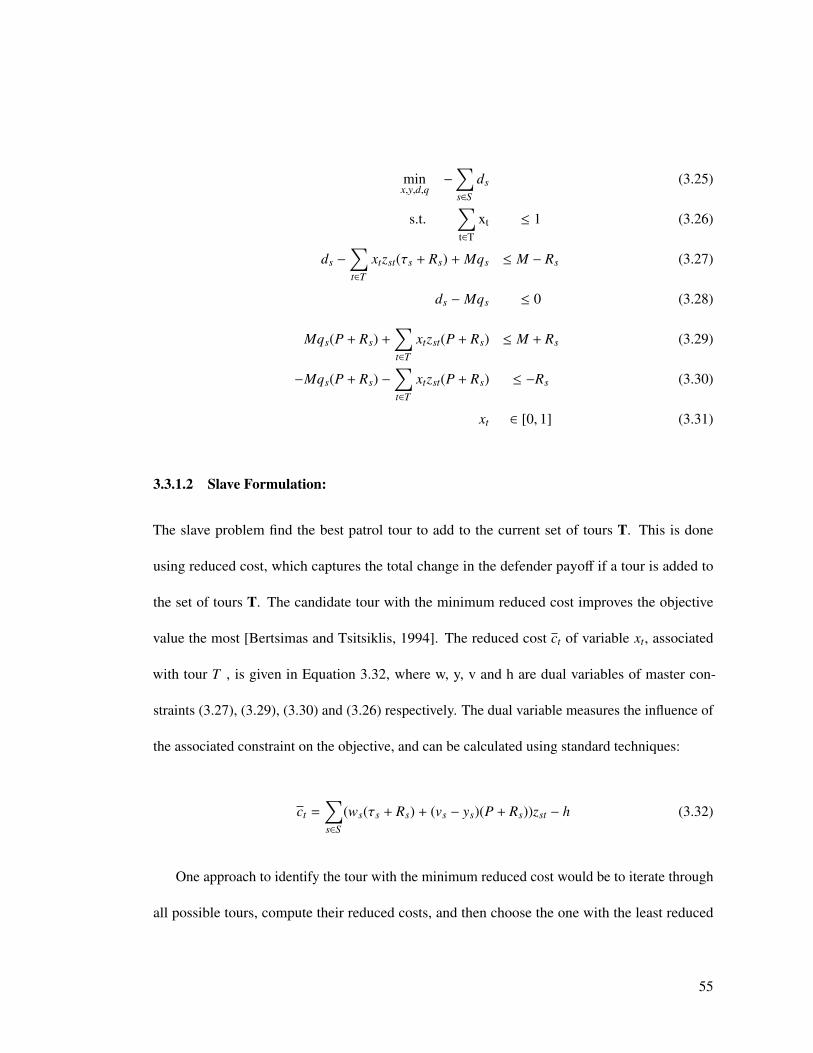
minx,y,d,q

−∑s∈S

ds (3.25)

s.t.∑t∈T

xt ≤ 1 (3.26)

ds −∑t∈T

xtzst(τs + Rs) + Mqs ≤ M − Rs (3.27)

ds − Mqs ≤ 0 (3.28)

Mqs(P + Rs) +∑t∈T

xtzst(P + Rs) ≤ M + Rs (3.29)

−Mqs(P + Rs) −∑t∈T

xtzst(P + Rs) ≤ −Rs (3.30)

xt ∈ [0, 1] (3.31)

3.3.1.2 Slave Formulation:

The slave problem find the best patrol tour to add to the current set of tours T. This is done

using reduced cost, which captures the total change in the defender payoff if a tour is added to

the set of tours T. The candidate tour with the minimum reduced cost improves the objective

value the most [Bertsimas and Tsitsiklis, 1994]. The reduced cost ct of variable xt, associated

with tour T , is given in Equation 3.32, where w, y, v and h are dual variables of master con-

straints (3.27), (3.29), (3.30) and (3.26) respectively. The dual variable measures the influence of

the associated constraint on the objective, and can be calculated using standard techniques:

ct =∑s∈S

(ws(τs + Rs) + (vs − ys)(P + Rs))zst − h (3.32)

One approach to identify the tour with the minimum reduced cost would be to iterate through

all possible tours, compute their reduced costs, and then choose the one with the least reduced

55

cost. However, we propose a minimum-cost integer network flow formulation that efficiently finds

the optimal column (tour). Feasible tours in the domain map to feasible flows in the network flow

formulation and vice-versa. The minimum cost network flow graph is constructed in the following

manner. A virtual source and virtual sink are constructed to mark the beginning and ending

locations, i.e. home base, for a defender tour. These two virtual nodes are directly connected by

an edge signifying the ”Not attack” option for the attacker. As many levels of nodes are added

to the graph as the number of targets. Each level contains nodes for every target. There are links

from every node on level i to every node to level i + 1. Each node on every level i is also directly

connected to the sink. Additionally, the length of the edge between any two nodes is the Euclidean

distance between the two corresponding targets. Constraints are added to the slave problem to

disallow a tour that covers two nodes corresponding to the same target (i.e. a network flow going

through node (1,1) and (2,1) in the figure would be disallowed since both these nodes correspond

to target 1). An additional constraint is added to the slave to ensure that the total length of every

flow (i.e. sum of lengths of edges with a non-zero flow) is less than the specified upper bound

L. Thus, the slave is setup such that there exists a one-to-one correspondence between a flow

generated by the slave problem and patrol route that the defender can undertake. Figure 3.3 shows

an example graph for the slave.

Each node representing a target is split into two dummy nodes with an edge between them.

Link costs are put on these edges. The costs on these graphs are defined by decomposing the

reduced cost of a tour, ct, into reduced costs over individual targets, cs. We decompose ct into

56

…

…

…

…

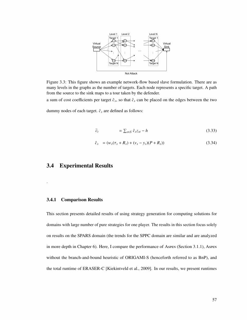
Target 1

Target N

…

Virtual Source

Virtual Sink

Not Attack

Target 1

Target N

Level 1 Level 2 Level N

(1,1)

(1,2)

(1,N)

(2,1)

(2,2)

(2,N)

(N,1)

(N,2)

(N,N)

Figure 3.3: This figure shows an example network-flow based slave formulation. There are asmany levels in the graphs as the number of targets. Each node represents a specific target. A pathfrom the source to the sink maps to a tour taken by the defender.

a sum of cost coefficients per target cs, so that cs can be placed on the edges between the two

dummy nodes of each target. cs are defined as follows:

ct =∑

s∈S cszst − h (3.33)

cs = (ws(τs + Rs) + (vs − ys)(P + Rs)) (3.34)

3.4 Experimental Results

.

3.4.1 Comparison Results

This section presents detailed results of using strategy generation for computing solutions for

domains with large number of pure strategies for one player. The results in this section focus solely

on results on the SPARS domain (the trends for the SPPC domain are similar and are analyzed

in more depth in Chapter 6). Here, I compare the performance of Aspen (Section 3.1.1), Aspen

without the branch-and-bound heuristic of ORIGAMI-S (henceforth referred to as BnP), and

the total runtime of ERASER-C [Kiekintveld et al., 2009]. In our results, we present runtimes

57

for ERASER-C that include the generation of the defender’s mixed strategy using our column

generation approach (refer Section 3.2) in order to provide a fair comparison with ASPEN. For

this experiment, we generate random instances of SPARS problems [Kiekintveld et al., 2009] with

schedules of size two organized in a bipartite graph, e.g. with one departure flight and one arrival

flight drawn from disjoint sets (this ensures that ERASER-C can find a correct optimal solution).

We vary the number of targets, defender resources, and schedules.

All experiments are based on 30 sample games, and problem instances that took longer than 30

minutes to run were terminated. The results of the first experiment are shown in Figure 3.4. The

y-axis shows the runtime in seconds on the log scale. The x-axis shows the number of resources.

These results shows that for low number of targets (less than 100), ERASER-C is the fastest

algorithm. However, ERASER-C starts to lose its performance advantage when the number of

targets is increased. BnP is the slowest (as expected), and scales much poorly as compared to the

other algorithms. To further examine the advantage offered by Aspen, we increased the number of

targets to 200 and beyond in the second set of experiments. The results varying the number of

defender resources for 200 targets are shown in Figure 3.5(a).

As seen in Figure 3.5, Aspen is the fastest of the three algorithms for large number of targets.

The effectiveness of the ORIGAMI-S bounds and branching are clear in the comparison with

standard BnP method. Since Aspen solves a far more general set of security games (SPARS), we

would not expect it to be competitive with ERASER-C in its specialized domain. However, Aspen

was 6 times faster than ERASER-C in some instances. This improvement over ERASER-C was an

unexpected trend, and can be attributed to the number of columns generated by the two approaches

(Table 3.1). We observe similar results in the second and third data sets presented in Figures 3.5(b)

and 3.5(c).

58

0.1  

1  

10  

100  

20   30   40   50   100   150  

Run,

me  (in

 secs)  

Targets  

Comparison  (10  Resources)  

ERASER  BnP  ASPEN  

Figure 3.4: Comparison between ERASER-C, Aspen and BnP for SPARS problem instances with10 resources. The number of schedules for these experiments was two times the number of targets.In this figure and others with y-axis on the log scale, error bars are not shown since they are notprominent because of the logarithmic axis. In this experiment, the difference in runtime for allpair-wise comparisons was statistically significant except between ERASER-C and Aspen for 40and 50 targets.

Resources ASPEN ERASER-C BnP (max. 30 mins)10 126 204 153220 214 308 167930 263 314 197640 227 508 151050 327 426 1393

Table 3.1: This table shows the average number of columns (pure strategies for the defender)generated by the column generation approach for all the three algorithms: Aspen, BnP, and columngeneration on marginals generated by ERASER-C. These results are averaged over 30 SPARSproblem instances, with 200 targets and 600 schedules where each schedule is of size 2. Theseresults confirm the presence of small support sets in such problem instances: the number of targetsin these experiments was 200 which implies that the maximum number of pure strategies can beof the order of 1016 for 10 resources up to 1047 for 50 resources.

3.4.2 ASPEN on Large SPARS Instances:

We also evaluate the performance of Aspen on arbitrary scheduling problems as the size of the prob-

lem is varied to include very large instances. No comparisons could be made because ERASER-C

does not handle arbitrary schedules and the only correct algorithms known, DOBSS [Paruchuri

59

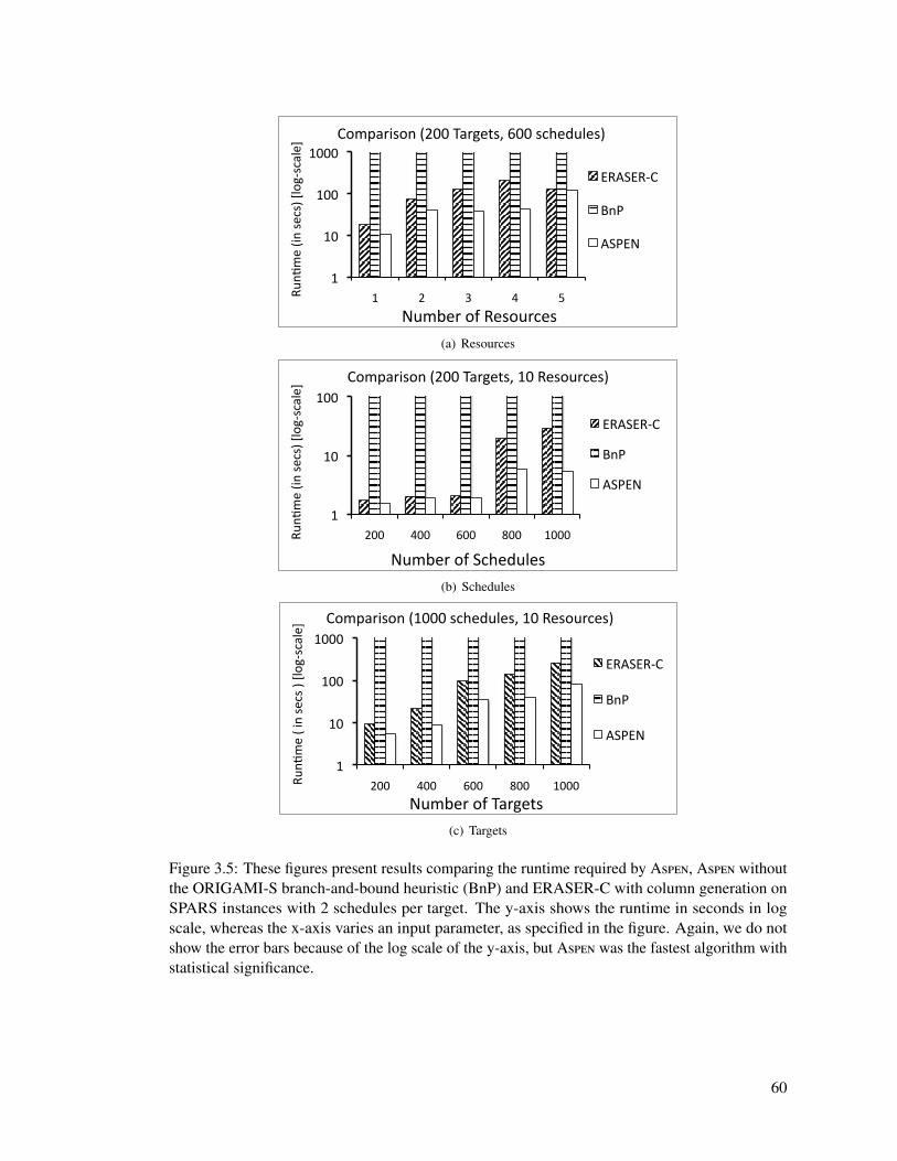
1  

10  

100  

1000  

1   2   3   4   5  Run+

me  (in

 secs)  [log-­‐scale]  

Number  of  Resources  

Comparison  (200  Targets,  600  schedules)  

ERASER-­‐C  

BnP  

ASPEN  

(a) Resources

1  

10  

100  

200   400   600   800   1000  Run+

me  (in

 secs)  [log-­‐scale]  

Number  of  Schedules  

Comparison  (200  Targets,  10  Resources)  

ERASER-­‐C  

BnP  

ASPEN  

(b) Schedules

1  

10  

100  

1000  

200   400   600   800   1000  Run+

me  (  in  secs  )  [lo

g-­‐scale]  

Number  of  Targets  

Comparison  (1000  schedules,  10  Resources)  

ERASER-­‐C  

BnP  

ASPEN  

(c) Targets

Figure 3.5: These figures present results comparing the runtime required by Aspen, Aspen withoutthe ORIGAMI-S branch-and-bound heuristic (BnP) and ERASER-C with column generation onSPARS instances with 2 schedules per target. The y-axis shows the runtime in seconds in logscale, whereas the x-axis varies an input parameter, as specified in the figure. Again, we do notshow the error bars because of the log scale of the y-axis, but Aspen was the fastest algorithm withstatistical significance.

60

et al., 2008a] and BnP (Aspen without the ORIGAMI-S branch-and-bound heuristic), do not scale

to these problem sizes. We vary the number of resources, schedules, and targets as before. In addi-

tion, we vary the number of targets per schedule for each of the three cases to test more complex

scheduling problems. Figure 3.6(a) shows the runtime results with 1000 feasible schedules and

200 targets, averaged over 10 samples. The x-axis shows the number of resources, and the y-axis

shows the runtime in seconds. Each line represents a different number of schedules per target.

The number of joint schedules in these instances can be as large as 1023 ((100010

)≈ 2.6 × 1023).

Interestingly, the runtime does not increase much when the number of resources is increased from

10 to 20 when there are 5 targets per schedules. Column 4 of Table 3.2 illustrates that the key

reason for constant runtime is that the average number of generated columns remains similar. For

a fixed number of resources, we observe an increase in runtime for more complex schedules that

corresponds with an increase in the number of columns generated. The other two experiments,

Figure 3.6(b) and 3.6(c) also show similar trends.

Resources 3 Targets / schedule 4 Targets / schedule 5 Targets / schedule5 456 518 65810 510 733 94115 649 920 109220 937 1114 1124

Table 3.2: This table shows the average number of columns (pure strategies for the defender)generated by the column generation approach for Aspen. These results are averaged over 30SPARS problem instances, with 200 targets and 1000 schedules.

61

0  

1000  

2000  

3000  

4000  

5000  

6000  

7000  

8000  

5   10   15   20  Ru

n.me  (in

 secon

ds)  

Number  of  Resources  

Scale-­‐up  (200  Targets,  1000  schedules)  

2  Targets/Schedule  3  Targets/Schedule  4  Targets/Schedule  5  Targets/Schedule  

(a) Resources

0  

5000  

10000  

15000  

20000  

25000  

50   500   1000   1500   2000  

Run)

me  (in

 secon

ds)  

Number  of  Schedules  

Scale-­‐up  (200  Targets,  10  Resources)  

2  Targets/Schedule  3  Targets/Schedule  4  Targets/Schedule  5  Targets/Schedule  

(b) Schedules

0  

1000  

2000  

3000  

4000  

5000  

6000  

7000  

8000  

50   100   150   200  

Run.

me  (in

 secon

ds)  

Number  of  Targets  

Scale-­‐up  (1000  schedules,  10  resources)  

2  Targets/Schedule  3  Targets/Schedule  4  Targets/Schedule  5  Targets/Schedule  

(c) Targets

Figure 3.6: These figures present the runtime results for Aspen when the size of the input problemis scaled. The y-axis shows the runtime in seconds, whereas the x-axis varies an input parameter,as specified in the figure.

62

Chapter 4: Strategy generation for both players

This chapter focuses on the network security domain (NSD), and shows how strategy generation

for both players can be used to compute solutions for extremely large problems with exponentially

many pure strategies for both the players. However, before I proceed to describe my algorithms,

Rugged and Snares, I first describe why Ranger, the best previous approach, failed to generate

correct solutions for NSD problem instances. The Ranger algorithm as used in this chapter is

described in Section 2.9.4.

4.1 Ranger Counterexample

Ranger was introduced by Tsai et al. [Tsai et al., 2010] and was designed to obtain approximate

solutions for the defender for the network security game. Its main component is a polynomial-

sized linear program that, rather than solving for a distribution over allocations, solves for the

marginal probability with which the defender covers each edge. It does this by approximating

the capture probability as the sum of the marginals along the attacker’s path. It further presents

some sampling techniques to obtain a distribution over defender allocations from these marginals.

What was known before was that the Ranger solution (regardless of the sampling method used) is

suboptimal in general, because it is not always possible to find a distribution over allocations such

63

that the capture probability is indeed the sum of marginals on the path. In this paper, we show that

Ranger’s error can be arbitrarily large.

Let us consider the example graph shown in Figure 4.1. This multi-graph1 has a single source

node, s, and two targets, t1 and t2; the defender has 2 resources. Furthermore, the payoffs T of the

targets are defined to be 1 and 2 for targets t1 and t2 respectively.

s t1 t2

a

a

a

b

Figure 4.1: This example is solved incorrectly by Ranger. The variables a, b are the coverageprobabilities on the corresponding edges.

Ranger solution:

Suppose Ranger puts marginal coverage probability a on each of the three edges between s and

t1,2 and probability b on the edge between t1 and t2, as shown in Figure 4.1. Ranger estimates that

the attacker gets caught with probability a when attacking target t1 and probability a + b when

attacking target t2. Ranger will attempt to make the attacker indifferent between the two targets to

obtain the minimax equilibrium. Thus, Ranger’s output is a = 3/5, b = 1/5, obtained from the

following system of equations:

1(1 − a) = 2(1 − (a + b)) (4.1)

3a + b = 2 (4.2)

1We use a multi-graph for simplicity. This counterexample can easily be converted into a similar counterexamplethat has no more than one edge between any pair of nodes in the graph.

2We can assume without loss of solution quality that symmetric edges will have equal coverage.

64

However, there can be no allocation of 2 resources to the edges such that the probability of the

attacker being caught on his way to t1 is 3/5 and the probability of the attacker being caught on

his way to t2 is 4/5. (The reason is that in this example, the event of there being a defensive

resource on the second edge in the path cannot be disjoint from the event of there being one on

the first edge.) In fact, for this Ranger solution, the attacker cannot be caught with a probability

of more than 3/5 when attacking target t2, and so the defender utility cannot be greater than

−2(1 − 3/5) = −4/5.

Optimal solution:

Figure 4.2 shows the six possible allocations of the defender’s two resources to the four edges.

Three of them block some pair of edges between s and t1. Suppose that each of these three

allocations is played by the defender with probability x.3 Each of the other three allocations blocks

one edge between s and t1 as well as the edge between t1 and t2. Suppose the defender chooses

these allocations with probability y each (refer Figure 4.2). The probability of the attacker being

x

x

x

y

y

y

t2t1s

t2t1s

t2t1s

t2t1s

t2t1s

t2t1s

Figure 4.2: The possible allocations of two resources to the four edges. The blocked edges areshown in bold. The probabilities (x or y) are shown next to each allocation.

caught on his way to t1 is 23 3x + 1

3 3y, or 2x + y. Similarly, the probability of the attacker being

3Again, this can be assumed without loss of generality for symmetric edges.

65

caught on his way to t2 is 2x + 3y. Thus, a minimax strategy for this problem is the solution of

Equations (4.3) and (4.4), which make the attacker indifferent between targets t1 and t2.

1(1 − 2x − y) = 2(1 − 2x − 3y) (4.3)

3x + 3y = 1 (4.4)

The solution to the above system is x = 2/9, y = 1/9, so that the expected attacker utility is 4/9.

Thus, the expected defender utility is −4/9, which is higher than the expected defender utility of at

most −4/5 resulting from using Ranger.

Ranger sub-optimality:

Suppose the payoff T (t2) of target t2 in the example above was H,H > 1. The Ranger solution in

this case, again obtained using Equations 4.1 and 4.2, would be a =(H+1)

(2H+1) , b =(H−1)

(2H+1) .

Then, consider an attacker who attacks the target t2 by first going through one of the three

edges from s to t1 uniformly at random (and then on to t2). The attacker will fail to be caught on

the way from t1 to t2 with probability (1 − b), given that the defender’s strategy is consistent with

the output of Ranger. Even conditional on this failure, the attacker will fail to be caught on the

way from s to t1 with probability at least 1/3, because the defender has only 2 resources. Thus, the

probability of a successful attack on t2 is at least (1 − b)(1/3), and the attacker’s best-response

utility is at least:

H(1 − b)3

=H(H + 2)3(2H + 1)

>H(H + 0.5)3(2H + 1)

=H6

(4.5)

Thus, the true defender utility for any strategy consistent with Ranger is at most −H6 .

66

Now, consider another defender strategy in which the defender always blocks the edge from t1

to t2, and also blocks one of the three edges between s and t1 uniformly at random. For such a

defender strategy, the attacker can reach t1 with probability 2/3, but cannot reach target t2 at all.

Thus, the attacker’s best-response utility in this case is 2/3. Therefore, the optimal defender utility

is at least −2/3. Therefore, any solution consistent with Ranger is at least H6 /

23 = H

4 suboptimal.

Since H is arbitrary, Ranger solutions can be arbitrarily suboptimal. This motivates our exact,

double-oracle algorithm, Rugged.

4.2 Rugged

In this section, I present Rugged, a double-oracle based algorithm for network security games. We

also analyze the computational complexity of determining best responses for both the defender

and the attacker, and, to complete the Rugged algorithm, we give algorithms for computing the

best responses.

4.2.1 Algorithm Description

The algorithm Rugged is presented as Algorithm 2. X is the set of defender allocations generated

so far, while A is the set of attacker paths generated so far. CoreLP(X,A) finds an equilibrium

(and hence, minimax and maximin strategies) of the two-player zero-sum game consisting of the

sets of pure strategies, X and A, generated so far. CoreLP returns x and a, which are the current

equilibrium mixed strategies for the defender and the attacker over X and A respectively. The

defender oracle (DO) generates a defender allocation Λ that is a best response for the defender

67

against a. (This is a best response among all allocations, not just those in X.) Similarly, the

attacker oracle (AO) generates an attacker path Γ that is a best response for the attacker against x.

Algorithm 2 Double Oracle for Urban Network Security1. Initialize X by generating arbitrary candidate defender allocations.2. Initialize A by generating arbitrary candidate attacker paths.repeat

3. (x, a)←CoreLP(X,A).4a. Λ← DO(a).4b. X← X ∪ {Λ}.5a. Γ← AO(x).5b. A← A ∪ {Γ}.

until convergence7. Return (x, a)

The double oracle algorithm thus starts with a small set of pure strategies for each player,

and then grows these sets in every iteration by applying the best-response oracles to the current

solution. Execution continues until convergence is detected. Convergence is achieved when the

best-response oracles of both the defender and the attacker do not generate a pure strategy that is

better for that player than the player’s strategy in the current solution (holding the other player’s

strategy fixed). In other words, convergence is obtained if, for both players, the reward given by

the best-response oracle is no better than the reward for the same player given by the CoreLP.

The correctness of best-response-based double oracle algorithms for two-player zero-sum

games has been established by McMahan et al [McMahan et al., 2003]; the intuition for this

correctness is as follows. Once the algorithm converges, the current solution must be an equilibrium

of the game, because each player’s current strategy is a best response to the other player’s current

strategy—this follows from the fact that the best-response oracle, which searches over all possible

strategies, cannot find anything better. Furthermore, the algorithm must converge, because at worst,

it will generate all pure strategies.

68

4.2.2 CoreLP

The purpose of CoreLP is to find an equilibrium of the restricted game consisting of defender pure

strategies X and attacker pure strategies A. Below is the standard formulation for computing a

maximin strategy for the defender in a two-player zero-sum game.

maxU∗d ,x

U∗d (4.6)

s.t. U∗d ≤ Ud(x, A j) ∀ j = 1, . . . , |A| (4.7)

1Tx = 1 (4.8)

x ∈ [0, 1]|X| (4.9)

The defender’s mixed strategy x, defined over X, and utility U∗d are the variables for this problem.

Inequality (4.7) is family of constraints; there is one constraint for every attacker path A j in A.

The function Ud(x, A j) is the expected utility of the attacker path A j. Given A j, the probability

that the attacker is caught is the sum of the probabilities of the defender allocations that would

catch the attacker. (We can sum these probabilities because they correspond to disjoint events.)

More precisely, let zi j be an indicator for whether allocation Xi intersects with path A j, that is,

zi j =

1 if Xi ∩ A j , ∅

0 otherwise(4.10)

These zi j are not variables of the linear program; they are parameters that are determined at the

time the best responses are generated. Then, the probability that an attacker playing path A j is

caught is∑

i zi jxi, and the probability that he is not caught is∑

i(1−zi j)xi. Thus, the payoff function

69

Ud(x, A j) for the defender for choosing a mixed strategy x when the attacker chooses path A j is

given by Equation (4.11), where T (t j) is the attacker’s payoff for reaching t j.

Ud(x, A j) = −T (t j) · (∑

i

(1 − zi j)xi) (4.11)

The dual variables corresponding to Inequality (4.7) give the attacker’s mixed strategy a,

defined over A. The expected utility for the attacker is given by −U∗d.

4.2.3 Defender Oracle

This section concerns the best-response oracle problem for the defender. The Defender Oracle

problem is stated as follows: generate the defender pure strategy (resource allocation) Λ allocating

k resources over the edges E that maximizes the defender’s expected utility against a given attacker

mixed strategy a over paths A.

Defender Oracle problem is NP-hard: We show this by reducing the set cover problem to it.

The Set-Cover problem: Given are a set U, a collection S of subsets of U (that is, S ⊆ 2U), and

an integer k. The question is whether there is a cover C ⊆ S of size k or less, that is,⋃

c∈C c = U

and |C| ≤ k. We will use a modification of this well-known NP-hard problem so that S always

contains all singleton subsets of U, that is, x ∈ U implies {x} ∈ S. This modified problem remains

NP-hard.

Theorem 2. The Defender Oracle problem is NP-hard, even if there is only a single source and a

single target.

Proof. Reduction from Set-Cover to Defender Oracle: We convert an arbitrary instance of the

set cover problem to an instance of the defender oracle problem by constructing a graph G with

70

just 3 nodes, as shown in Figure 4.3. The graph G is a multi-graph4 with just three nodes, so that

N = {s, v, t}, where s is the only source and t is the only target (with arbitrary positive value). There

are up to |S| loop edges adjacent to node v; each loop edge corresponds to a unique non-singleton

subset in S. There are |U | edges between s and v, each corresponding to a unique element in

U. There are also |U | edges between v and t, each corresponding to a unique element in U. The

attacker’s paths correspond to the elements in U. A path that corresponds to u ∈ U starts with

the edge between s and v that corresponds to u, then loops through all the edges that correspond

to non-singleton subsets in S that contain u, and finally ends with the edge between v and t that

corresponds to u. Hence, any two paths used by the attacker can only intersect at the loop edges.

The probabilities that the defender places on these paths are arbitrary positive numbers. We now

e2

e1

e3

e1'

e2'

e3'e1,2

e1,3

s v t

Figure 4.3: A defender oracle problem instance corresponding to the SET-COVER instance withU = {1, 2, 3}, S = {{1}, {2}, {3}, {1, 2}, {1, 3}}. Here, the attacker’s mixed strategy uses three paths:(e1, e1,2, e1,3, e′1), (e2, e1,2, e′2), (e3, e1,3, e′3). Thus, the SET-COVER instance has a solution of size2 (for example, using {1, 2} and {1, 3}); correspondingly, with 2 resources, the defender can alwayscapture the attacker (for example, by covering e1,2, e1,3).

show that set U can be covered with k subsets in S ⊆ 2U if and only if the defender can block all

of the attacker’s paths with k resources in the corresponding defender oracle problem instance.

The “if” direction: If the defender can block all the paths used by the attacker with k

resources, then the set U can be covered with C ⊆ S, where |C| = k and is constructed as follows.

If the defender places a resource on a loop edge, then C includes the non-singleton subset in S

4Having a multi-graph is not essential to the NP-hardness reduction.

71

that corresponds to that loop edge. If the defender blocks any other edge then C includes the

corresponding singleton subset.

The “only if” direction: If there exists a cover C of size k, then the defender can block all

the paths by placing a defensive resource on every loop edge that corresponds to a non-singleton

subset in C, and placing a defensive resource on the corresponding edge out of s for every singleton

subset in C. �

Formulation: The defender oracle problem, described below, can be formulated as a mixed

integer linear program (MILP). The objective of the MILP is to identify the allocation that covers as

many attacker paths as possible, where paths are weighted by the product of the payoff of the target

attacked by the path and probability of attacker choosing it. (In this formulation, probabilities

a j are not variables; they are provided by CoreLP.) In the formulation, λe = 1 indicates that we

assign a resource to edge e, and z j = 1 indicates that path A j (refer Table 2.9) is blocked by the

allocation.

maxz,λ

−∑

j(1 − z j)a jTt j (4.12)

s.t. z j ≤∑

e

A jeλe (4.13)

∑e λe ≤ k (4.14)

λe ∈ {0, 1} (4.15)

z j ∈ [0, 1] (4.16)

Theorem 3. The MILP described above correctly computes a best-response allocation for the

defender.

72

Proof. The defender receives a payoff of −T (t j)a j if the attacker successfully attacks target t j

using path A j, and 0 in the case of an unsuccessful attack. Hence, if we make sure that 1 − z j = 1

if path A j is not blocked, and 0 otherwise, then the objective function (4.12) correctly models the

defender’s expected utility. Inequality (4.13) ensures this: its right-hand side will be at least 1

if there exists an edge on the path A j that defender is covering, and 0 otherwise. z j need not be

restricted to take an integer value because the objective is increasing with z j and if the solver can

push it above 0, it will choose to push it all the way up to 1. Therefore, if we let Λ correspond to

the set of edges covered by the defender, z j will be set by the solver so that:

z j =

1 if Λ ∩ A j , ∅⇔ ∃e |λe = A je = 1

0 otherwise(4.17)

Inequality (4.14) enforces that the defender covers at most as many edges as the number of

available resources k, and thus ensures feasibility. Hence, the above MILP correctly captures the

best-response oracle problem for the defender. �

Proposition 1. For any attacker mixed strategy, the defender’s expected utility from the best

response provided by the defender oracle is no worse than the defender’s equilibrium utility in the

full zero-sum game.

Proof. In any equilibrium, the attacker plays a mixed strategy that minimizes the defender’s

best-response utility; therefore, if the attacker plays any other mixed strategy, the defender’s

best-response utility can be no worse. �

73

4.2.4 Attacker Oracle

This section concerns the best-response oracle problem for the attacker. The Attacker Oracle

problem is to generate the attacker pure strategy (path) Γ from some source s ∈ S to some target

t ∈ T that maximizes the attacker expected utility given the defender mixed strategy x over

defender allocations X.

Attacker Oracle is NP-hard: We show that the attacker oracle problem is also NP-hard by

reducing 3-SAT to it.

Theorem 4. The Attacker Oracle problem is NP-hard, even if there is only a single source and a

single target.

Proof. Reduction from 3-SAT to Attacker Oracle: We convert an arbitrary instance of 3-SAT

to an instance of the attacker oracle problem as follows. Suppose the 3-SAT instance contains n

variables xi, i = 1, . . . , n, and k clauses. Each clause is a disjunction of three literals, where each

literal is either a variable or the negation of the variable. Consider the following example:

E = (x1 ∨ ¬x2 ∨ ¬x3) ∧ (x1 ∨ x2 ∨ x4) (4.18)

The formula E contains n = 4 variables and k = 2 clauses.

We construct a multi-graph G5 with n + k + 1 nodes, v0, . . . , vn+k so that the source node is

s = v0, and the target node is t = vn+k. Every edge connects some pair of nodes with consecutive

indices, so that every simple path from s to t contains exactly n + k edges. Each edge corresponds

to a literal in the 3-SAT expression (that is, either xi or ¬xi). There are exactly three edges that

connect nodes vi−1 and vi for i = 1, . . . , k. Those three edges correspond to the three literals in the5We use a multi-graph for simplicity; having a multi-graph is not essential for the NP-hardness reduction.

74

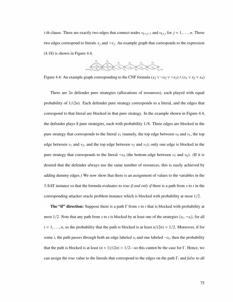
i-th clause. There are exactly two edges that connect nodes vk+ j−1 and vk+ j for j = 1, . . . , n. Those

two edges correspond to literals x j and ¬x j. An example graph that corresponds to the expression

(4.18) is shown in Figure 4.4.

x1

x1

x4

x1

¬x1

x2

¬x2

x3

¬x3

x4

¬x4

¬x2

¬x3

x2

s=v0

v1

v2

v3

v4

v5 v

6=t

Figure 4.4: An example graph corresponding to the CNF formula (x1 ∨¬x2 ∨¬x3)∧ (x1 ∨ x2 ∨ x4)

There are 2n defender pure strategies (allocations of resources), each played with equal

probability of 1/(2n). Each defender pure strategy corresponds to a literal, and the edges that

correspond to that literal are blocked in that pure strategy. In the example shown in Figure 4.4,

the defender plays 8 pure strategies, each with probability 1/8. Three edges are blocked in the

pure strategy that corresponds to the literal x1 (namely, the top edge between v0 and v1, the top

edge between v1 and v2, and the top edge between v2 and v3); only one edge is blocked in the

pure strategy that corresponds to the literal ¬x4 (the bottom edge between v5 and v6). (If it is

desired that the defender always use the same number of resources, this is easily achieved by

adding dummy edges.) We now show that there is an assignment of values to the variables in the

3-SAT instance so that the formula evaluates to true if and only if there is a path from s to t in the

corresponding attacker oracle problem instance which is blocked with probability at most 1/2.

The “if” direction: Suppose there is a path Γ from s to t that is blocked with probability at

most 1/2. Note that any path from s to t is blocked by at least one of the strategies {xi,¬xi}, for all

i = 1, . . . , n, so the probability that the path is blocked is at least n/(2n) = 1/2. Moreover, if for

some i, the path passes through both an edge labeled xi and one labeled ¬xi, then the probability

that the path is blocked is at least (n + 1)/(2n) > 1/2—so this cannot be the case for Γ. Hence, we

can assign the true value to the literals that correspond to the edges on the path Γ, and false to all

75

the other literals. This must correspond to a solution to the 3-SAT instance, because each clause

must contain a literal that corresponds to an edge on the path, and is thus assigned a true value.

The “only if” direction: Suppose there is an assignment of values to the variables such that

the 3-SAT formula evaluates to true. Consider a simple path Γ that goes from s to t through edges

that correspond to literals with true values in the assignment. Such a path must exist because

by assumption the assignment satisfies every clause. Moreover, this path is blocked only by the

defender strategies that correspond to true literals, of which there are exactly n. So the probability

that the path is blocked is n/(2n) = 1/2. �

Formulation: The attacker oracle problem can be formulated as a set of mixed integer linear

programs, as described below. For every target in T , we solve for the best path to that target; then

we take the best solution overall. Below is the formulation when the attacker is attacking target

tm. (In this formulation, probabilities xi are not variables; they are values produced earlier by

CoreLP.) In the formulation, γe = 1 indicates that the attacker passes through edge e, and zi = 1

76

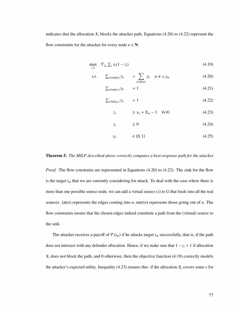
indicates that the allocation Xi blocks the attacker path. Equations (4.20) to (4.22) represent the

flow constraints for the attacker for every node n ∈ N.

maxz,γ

Ttm∑

i xi(1 − zi) (4.19)

s.t.∑

e∈out(n) γe =∑

e∈in(n)

γe n , s, tm (4.20)

∑e∈out(s) γe = 1 (4.21)

∑e∈in(tm) γe = 1 (4.22)

zi ≥ γe + Xie − 1 ∀e∀i (4.23)

zi ≥ 0 (4.24)

γe ∈ {0, 1} (4.25)

Theorem 5. The MILP described above correctly computes a best-response path for the attacker.

Proof. The flow constrains are represented in Equations (4.20) to (4.22). The sink for the flow

is the target tm that we are currently considering for attack. To deal with the case where there is

more than one possible source node, we can add a virtual source (s) to G that feeds into all the real

sources. in(n) represents the edges coming into n, out(n) represents those going out of n. The

flow constraints ensure that the chosen edges indeed constitute a path from the (virtual) source to

the sink.

The attacker receives a payoff of T (tm) if he attacks target tm successfully, that is, if the path

does not intersect with any defender allocation. Hence, if we make sure that 1− zi = 1 if allocation

Xi does not block the path, and 0 otherwise, then the objective function (4.19) correctly models

the attacker’s expected utility. Inequality (4.23) ensures this: if the allocation Xi covers some e for

77

which γe = 1, then it will force zi to be set at least to 1; otherwise, zi only needs to be set to at

least 0 (and in each case, the solver will push it all the way down to this value, which also explains

why the zi variables do not need to be restricted to take integer values). Therefore, if we let Γ

correspond to the path chosen by the attacker, zi will be set by the solver so that

zi =

1 if Xi ∩ Γ , ∅⇔ ∃e |γe = Xie = 1

0 otherwise(4.26)

It follows that the MILP objective is correct. Hence, the above MILP captures the best-response

oracle problem for the attacker. �

Proposition 2. For any defender mixed strategy, the attacker’s expected utility from the best

response provided by the attacker oracle is no worse than the attacker’s equilibrium utility in the

full zero-sum game.

Proof. In any equilibrium, the defender plays a mixed strategy that minimizes the attacker’s

best-response utility; therefore, if the defender plays any other mixed strategy, the attacker’s

best-response utility can be no worse. �

Figure 4.5: Example graph of Southern Mumbai with 455 nodes. Sources are depicted as greenarrows and targets are red bulls-eyes. Best viewed in color.

78

4.3 Evaluation of Rugged

In this section, we describe the results I achieved with Rugged. We conducted experiments on

graphs obtained from road network GIS data for the city of Mumbai (inspired by the 2008 Mumbai

incidents [Chandran and Beitchman, 29 November 2008]), as well as on artificially generated

graphs. We provide two types of results: (1) Firstly, we compare the solution quality obtained from

Rugged with the solution quality obtained from Ranger. These results are shown in Section 4.3.1.

(2) Secondly, we provide runtime results showing the performance of Rugged when the input

graphs are scaled up.6 The following three types of graphs were used for the experimental results:

(1) Weakly fully connected (WFC) graphs, denoted GWFC(N, E), are graphs where N is an

ordered set of nodes {n1, . . . , nm; S = {n1},T = {nm}}. For each node ni, there exists a set of

directed edges, {(ni, n j)|ni < n j}, in E. These graphs were chosen because of the extreme size of

the strategy spaces for both players. Additionally, there are no bottleneck edges, so these graphs

are designed to be computationally challenging for Rugged.

(2) Braid-type graphs, denoted GB(N, E), are graphs where N is a sequence of nodes n1 to

nm such that each pair ni−1 and ni is connected by 2 to 3 edges. Node n1 is the source node. Any

following node is a target node with probability 0.2, with payoff T randomly chosen between 1

and 100. These graphs have a similar structure as the graph in Figure 4.1, and were motivated by

the counterexample in Section 4.1.

(3) City graphs of different sizes were extracted from the southern part of Mumbai using the

GIS data provided by OpenStreetMaps. The placement of 2-4 targets was inspired by the Mumbai

incidents from 2008 [Chandran and Beitchman, 29 November 2008]; 2-4 sources were placed

6All experiments were run on standard desktop 2.8GHz machine with 2GB main memory.

79

on the border of the graph,7 simulating an attacker approaching from the sea. We ran the test for

graphs with the following numbers of nodes: 45, 129 and 252. Figure 4.5 shows a sample Mumbai

graph with 252 nodes, 4 sources and 3 targets.

4.3.1 Comparison with RANGER

This section compares the solution quality of Rugged and Ranger. Although we have already

established that Ranger solutions can be arbitrarily bad in general, the objective of these tests is to

compare the actual performance of Ranger with Rugged. The results are given in Table 4.1, which

shows the average and maximum error from Ranger. We evaluated Ranger on the three types of

graphs — city graphs, braid graphs and weakly fully connected graphs of different sizes, fixing

the number of defender resources to 2 and placing 3 targets, with varied values from the interval

[0, 1000]. The actual defender utility from the solution provided by Ranger8 is computed by using

the best-response oracle for the attacker with the Ranger defender strategy as input. The error of

Ranger is then expressed as the difference between the defender utilities in the solutions provided

by Ranger and by Rugged.

Table 4.1 shows the comparison results between Ranger and Rugged, summarized over 30

trials. It shows the percentage of trials in which Ranger gave an incorrect solution (denoted “pct”).

It also shows the average and maximum error of Ranger (denoted as avg and max respectively)

over these trials. It shows that while Ranger was wrong only about 1/3 of the time for Braid

graphs, it gave the wrong answer in all the runs on the fully connected graphs. Furthermore, it was

wrong 90% of the time on city graphs, with an average error of 215 units and a maximum error of

7We placed more sources and targets into larger graphs.8Because Ranger provides a solution in the form of marginal probabilities of defender allocations along edges, we

used Comb sampling [Tsai et al., 2010] to convert this into a (joint) probability distribution over defender allocations.

80

721 units. Given an average target value of 500, these are high errors indeed — indicating that

Ranger is unsuitable for deployment in real-world domains.

City Braid WFCnodes 45 129 10 20 10 20

avg error 215 250 210 259 191 80max error 721 489 472 599 273 117

pct 90% 100% 30% 37% 100% 100%avg T 500 500 500 500 500 500

Table 4.1: Ranger average and maximum error and percent of samples where Ranger provided asuboptimal solution. Target values T were randomly drawn from the interval [1, 1000].

(a) (b)

(c)

Figure 4.6: Results. Figure (a) shows the scale-up analysis on WFC graph of different sizes. Figure(b) shows the convergence of oracle values to the final game value and the anytime bounds. Figure(c) compares the runtimes of oracles and the core LP.

4.3.2 Scale-up and analysis

This section concerns the performance of Rugged when the input problem instances are scaled

up. The experiments were conducted on graphs derived directly from portions of Mumbai’s road

network. The runtime results are shown in Table 4.2, where the rows represent the size of the

81

1 2 3 445 0.91 6.43 22.58 33.42129 6.63 32.55 486.48 3140.23252 17.19 626.25 2014.14 34344.70

Table 4.2: Runtime (in seconds) of Rugged when the input problem instances are scaled up. Thesetests were done on graphs extracted from the road network of Mumbai. The rows correspond tothe number of nodes in the graph whereas the columns correspond to the number of defenderresources.

graph and the columns represent the number of defender resources that need to be scheduled. As

an example of the complexity of the graph, the number of attacker paths in the Mumbai graph with

252 nodes is at least a 1012, while the number of defender allocations is approximately 1010 for 4

resources. The game matrix for this problem cannot even be represented, let alone solved. The

ability of Rugged to compute optimal solutions in such situations, while overcoming NP-hardness

of both oracles, marks a significant advance in the state of the art in deploying game-theoretic

techniques.

Figure 4.6(a) examines the performance of Rugged when the size of the strategy spaces for

both players is increased. These tests were conducted on WFC graphs, since they are designed

to have large strategy spaces. These problems have 20 to 100 nodes and up to 5 resources. The

x-axis in the figure shows the number of nodes in the graph, while the y-axis shows the runtime in

seconds. Different number of defender resources are represented by different curves in the graph.

For example for 40 nodes, and 5 defender resources, Rugged took 108 seconds on average.

To speed up the convergence of Rugged, we tried to warm-start the algorithm with an initial

defender allocation such as min-cut-based allocations, target- and source-centric allocations,

RANGER allocations and combinations of these. No significant improvement of runtime was

measured; in some cases, the runtime increased because of the larger strategy set for the defender.

82

4.3.3 Algorithm Dynamics Analysis

This section analyzes the anytime solution quality and the performance of each of the three

components of Rugged: the defender oracle, the attacker oracle, and the CoreLP. When we solve

the best-response oracle problems, they provide lower and upper bounds on the optimal defender

utility, as shown in Propositions 1 and 2. Figure 4.6(b) shows the progress of the bounds and

the CoreLP solution for a sample problem instance scheduling 2 defender resources on a fully

connected network with 50 nodes. The x-axis shows the number of iterations and the y-axis

shows the expected defender utility. The graph shows that a good solution (i.e., one where the

difference in the two bounds is less than ε) can be computed reasonably quickly, even though

the algorithm takes longer to converge to the optimal solution. For example, a solution with

an allowed approximation of 10 units9 can be computed in about 210 iterations, whereas 310

iterations are required to find the optimal solution. The difference between these two bounds gives

an upper bound on the error in the current solution of the CoreLP; this also provides us with an

approximation variant of Rugged.

Figure 4.6(c) compares the runtime needed by the three modules in every iteration. The x-axis

shows the iteration number and the y-axis shows the runtime in seconds in logarithmic scale. As

expected, CoreLP — solving a standard linear program — needs considerably less time in each

iteration than both the oracles, which solve mixed-integer programs. The figure also shows that

the modules scale well as the number of iterations increases.910 units is 1% of the maximum target payoff (1000).

83

4.4 Snares

The focus of this section is to present Snares (Securing Networks by Applying a Randomized

Emplacement Strategy), a new algorithm for computing the optimal solution for much larger

network security domains. Snares builds on the double-oracle approach of Rugged, and has

two novel features. First, Snares uses greedy heuristics to compute “better” (rather than “best”)

responses for both players. I show that the best-response problem for the defender has a sub-

modularity property, and exploiting this provide a bound for the solution quality of our better

response. Second, Snares uses a novel “mincut-fanout” technique to warm-start the computation

by initializing the game matrix with pure strategies for both the players. We show that naıve

ways of warm-starting the computation can actually increase the runtime, and that our novel

technique is effective. We extensively analyze these individual components of Snares in this paper.

Finally, I demonstrate Snares’s significant advance over the state-of-the-art (i.e., Rugged): whereas

state-of-the-art was restricted to the southern tip of Mumbai, with Snares, optimal strategies for

the entire road network of the city of Mumbai (refer Figure 4.7) can be obtained in a reasonable

amount of time.

4.4.1 Algorithm Description

I now present Snares in detail. The flow chart for Snares is presented in Figure 4.8. The boxes

with double lines are the three novel features in Snares, and I will describe them in detail in this

section, while modules also present in Rugged are shown in boxes with single-line borders. The

formal algorithm is given as Algorithm 3.

84

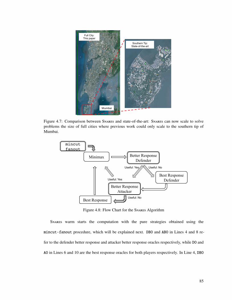
Southern Tip: State-of-the-art

Full City: This paper

Mumbai  

Figure 4.7: Comparison between Snares and state-of-the-art: Snares can now scale to solveproblems the size of full cities where previous work could only scale to the southern tip ofMumbai.

Minimax

Best Response Defender

Best Response

Better Response Defender

Better Response Attacker

Useful: Yes Useful: No

Useful: Yes

Useful: No

mincut!fanout!

Figure 4.8: Flow Chart for the Snares Algorithm

Snares warm starts the computation with the pure strategies obtained using the

mincut-fanout procedure, which will be explained next. DBO and ABO in Lines 4 and 8 re-

fer to the defender better response and attacker better response oracles respectively, while DO and

AO in Lines 6 and 10 are the best response oracles for both players respectively. In Line 4, DBO

85

Algorithm 3 Snares (G, k)1: Initialize X,A using mincut-fanout2: repeat3: (x, a)←CoreLP(X,A).4: X ← DBO(a).5: if Ud(X, a) − Ud(x, a) ≤ ε then6: X ← DO(a).7: X← X ∪ {X}.8: A← ABO(x).9: if Ua(A, x) − Ua(a, x) ≤ ε then

10: A← AO(x).11: A← A ∪ {A}.12: until convergence13: return (x, a)

returns a heuristic response X of the defender (we call this heuristic response as a “better” response

as opposed to the “best” response; here X may not be strictly better than existing strategies). Line 5

checks whether this utility Ud(X, a) is higher than the utility Ud(x, a) obtained from minimax by

at least ε, i.e., whether X is at least ε-better than all strategies present in X against a. If Ud(X, a) is

not at least ε higher than Ud(x, a), then the best response DO is invoked (Line 6). Line 7 guarantees

that each iteration adds an improving pure strategy to X, should one exist. Similarly computation

is performed for the attacker in Lines 8–11. Line 12 states that the computation proceeds until

convergence, which is obtained when the utility obtained from the best response of each player

is not better than the corresponding player’s utility from the minimax strategy. In other words,

convergence is obtained when Ud(X, a) − Ud(x, a) ≤ τ and Ua(A, x) − Ua(a, x) ≤ τ, where τ

defines the tolerance.10 Finally, Snares is guaranteed to converge on the global optimal solution

since convergence can be obtained only when the best responses for both the players are unable to

generate an improving strategy.

10In all our experiments, we fix both ε and τ to 0.001.

86

4.4.2 Warm-starting using mincut-fanout

The objective of warm-starting is to generate pure strategies for both the defender and the attacker

before the computation of the minimax strategy is started. Given the setup of the game, the best

response of the attacker will choose to attack the highest-valued target t with probability 1.0, if

there exists a s − t path in G(N, E) that does not intersect with any of the defender’s allocations.

Consequently, strategies considering the most-valued target get generated by the iterative procedure

of the double-oracle based algorithm in the first few iterations. The objective of warm-starts here

is to generate such strategies for both players and add them before the start of the double-oracle

iterative procedure. This will reduce the number of iterations that are required by the algorithm.

Thus, we construct a game with just one target: t. Solution for this game can be computed

in polynomial-time: it is to uniformly distribute the defender’s resources on the s − t min-

cut [Washburn and Wood, 1995]. Thus, mincut-fanout will sample pure strategies for the

defender, or defender allocations, from the s − t min-cut, such that each allocation covers k edges.

We then compute pure strategies for the attacker, or attacker paths, which are best responses to

each individual defender allocation. This is done using Dijkstra’s shortest path computation, such

that each edge e in the defender allocation X has weight inf, while the other edges have a weight

of 1. This also prefers short attacker paths over long ones, the intuition being that shorter paths

should be preferred by the attacker since longer paths are more likely to be intercepted.

We also generalized the above idea to consider all the targets and not just the highest valued

target t. However, as we show in Section 4.4.4.1, our choice of using only the highest valued

target in mincut-fanout performs better against considering all the targets. We also show that it

performs better against other potential strategies for warm starting the computation.

87

4.4.3 Using ”Better” Responses

Snares presents heuristics to compute “better responses” for both players. Each better response

module aims to compute a strategy for the corresponding player that is better than any strategy

already in the mix against the other player’s current equilibrium strategy. If successful, this

guarantees that CoreLP will compute a different equilibrium when this strategy is added. If the

better response heuristic fails to generate such a strategy, then the best-response module is called.

The objective is to reduce the number of invocations of the best response modules, both of which

solve an NP-hard problem [Jain et al., 2011b] and consume significant runtime when the problem

size gets bigger. On the other hand, the better response solutions used by Snares can be computed

in polynomial time. Furthermore, even with the use of better responses, Snares still converges on

the global equilibrium since the best responses modules are called if the better response modules

do not generate an improving strategy. We now present the better response algorithms for both

players.

4.4.3.1 Better Response for the Defender

In this section, we first present a greedy approach to generate the better response Xg of the defender.

This approach greedily maximizes a “normalized” defender utility function f (X, a). We next show

that this utility function is a non-negative sub-modular function, and then establish a bound on

the solution quality of our greedy better response solution. This bound suggests that our greedy

approach generates good solutions.

88

The defender payoffs are always negative in our domain: the defender gets a payoff of −T (t)

when the attacker successfully attacks target t and 0 otherwise. To facilitate analysis, we define a

non-negative normalized utility function f for the defender, where

Ud(X, a) = −∑

A j∈A|X∩A j=∅ a jT (t j) (4.27)

fa(X) = Ud(X, a) − Ud(∅, a) (4.28)

More specifically, f gives the added benefit of the defender allocation X over the defender not

protecting any edges. Furthermore, using Equation 4.27,

fa(X) = −∑

A j∈A|X∩A j=∅

a jT (t( j)) − Ud(∅, a) =∑

A j∈A|X∩A j,∅

a jT (t j) (4.29)

The greedy better response algorithm is described as Algorithm 4, where in each iteration,

the objective is to add an edge e to the greedy defender allocation Xg that maximizes fa(X ∪ {e}).

Here, Xg (Line 1) is the computed better response of the defender. a is the mixed strategy of the

attacker over the set of paths A that is input to the better response oracle. Ar in Line 2 is used to

keep track of attacker paths that not already covered by the defender’s allocation. we (initialized in

Line 4) represents the weight of each edge. These weights are updated in Lines 5–7, such that we

represents the total marginal usage of edge e in the attacker’s mixed strategy a, weighted by the

payoff of the target attacked by the attacker when traversing through e. The defender, following

the greedy approach, chooses an edge e∗ with the highest weight in Line 8. Finally, all the paths

intersecting with edge e∗ are removed from the set of paths considered in subsequent iterations,

89

i.e., from Ar (Lines 10–12). Lines 13–15 are invoked only if the allocation Xg already intersects

with all the attacker paths A j ∈ A, and ensures that the defender chooses k edges in its allocation.

Algorithm 4 Defender Better Response: DBO(A, a)1: Initialize Xg ← ∅ (defender allocation)2: Initialize Ar ← A3: while |Xg| < k and Ar , ∅ do4: we = 0 ∀e ∈ E5: for all A j ∈ Ar do6: for all e ∈ A j do7: we ← we + a jT (t( j))8: e∗ ← arg maxe we

9: Xg ← Xg ∪ {e∗}10: for all A j ∈ Ar do11: if e∗ ∈ A j then12: Ar ← Ar − {A j}

13: while |Xg| < k do14: Choose e arbitrarily from E15: Xg ← Xg ∪ e16: return Xg

Theorem 6. The normalized defender utility, fa(X), is sub-modular in X.

Proof. We show here that the gain in defender utility when adding an edge e to an existing defender

allocation X exhibits diminishing returns. Let X1 and X2 be two defender allocations such that

X1 ⊆ X2 ⊆ E. Furthermore, let A1 = {A j|A j ∩ X1 = ∅}, i.e., the set of attacker paths that are not

covered by X1. Similarly, let A2 = {A j|A j ∩ X2 = ∅}. Furthermore, X1 ⊆ X2, therefore, A2 ⊆ A1

since every path that is covered by X1 is covered by X2.

Moreover, using Equation 4.29,

fa(Xi) = −∑

A j∈Ai

a jT (t( j)) − Ud(∅, a), i ∈ {1, 2} (4.30)

90

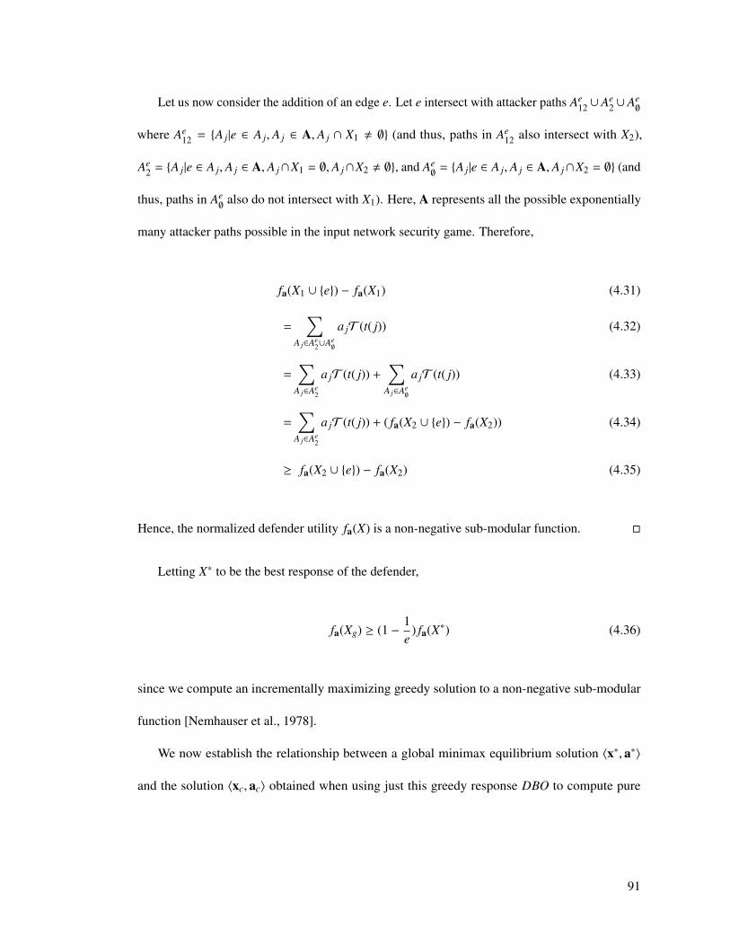
Let us now consider the addition of an edge e. Let e intersect with attacker paths Ae12 ∪Ae

2 ∪Ae∅

where Ae12 = {A j|e ∈ A j, A j ∈ A, A j ∩ X1 , ∅} (and thus, paths in Ae

12 also intersect with X2),

Ae2 = {A j|e ∈ A j, A j ∈ A, A j∩X1 = ∅, A j∩X2 , ∅}, and Ae

∅= {A j|e ∈ A j, A j ∈ A, A j∩X2 = ∅} (and

thus, paths in Ae∅

also do not intersect with X1). Here, A represents all the possible exponentially

many attacker paths possible in the input network security game. Therefore,

fa(X1 ∪ {e}) − fa(X1) (4.31)

=∑

A j∈Ae2∪Ae

∅

a jT (t( j)) (4.32)

=∑

A j∈Ae2

a jT (t( j)) +∑

A j∈Ae∅

a jT (t( j)) (4.33)

=∑

A j∈Ae2

a jT (t( j)) + ( fa(X2 ∪ {e}) − fa(X2)) (4.34)

≥ fa(X2 ∪ {e}) − fa(X2) (4.35)

Hence, the normalized defender utility fa(X) is a non-negative sub-modular function. �

Letting X∗ to be the best response of the defender,

fa(Xg) ≥ (1 −1e

) fa(X∗) (4.36)

since we compute an incrementally maximizing greedy solution to a non-negative sub-modular

function [Nemhauser et al., 1978].

We now establish the relationship between a global minimax equilibrium solution 〈x∗, a∗〉

and the solution 〈xc, ac〉 obtained when using just this greedy response DBO to compute pure

91

strategies for the defender, i.e., we never call DO but we do call AO by taking out Lines 5 and 6

from Algorithm 3 to arrive at 〈xc, ac〉.

Theorem 7. The defender utility Ud(xc, ac) is lower bounded by (1 − 1e )Ud(x∗, a∗) + 1

e Ud(∅, ac).

Proof. Firstly, given that 〈x∗, a∗〉 is a minimax solution,

Ud(x∗, a∗) ≥ Ud(x, a∗) ∀x (4.37)

Ud(x∗, a) ≥ Ud(x∗, a∗) ∀a (4.38)

Furthermore, defining

fa(x) =∑Xi∈X

xi fa(Xi) (4.39)

and using Equations (4.28), (4.37), (4.38) and (4.39), we have:

fa∗(x∗) ≥ fa∗(x) ∀x (4.40)

fa(x∗) ≥ fa∗(x∗) + (Ud(∅, a∗) − Ud(∅, a)) ∀a (4.41)

Therefore, using Equations (4.36) and (4.41),

fac(xc) = fac(DBO(ac)) (4.42)

≥ (1 −1e

) fac(DO(ac)) (4.43)

≥ (1 −1e

) fac(x∗) (by definition of DO) (4.44)

≥ (1 −1e

)[ fa∗(x∗) + (Ud(∅, a∗) − Ud(∅, ac))] (4.45)

Therefore, Ud(xc, ac) ≥ (1 − 1e )Ud(x∗, a∗) + 1

e Ud(∅, ac). �

92

Thus, not only is the better response defender utility bounded in each iteration, but the

solution quality for using just the better response is also bounded at convergence. Furthermore,

Ud(xc, ac) ≥ Ud(xc, a) ∀a. Thus, Ud(xc, ac) is the utility that xc guarantees the defender. Also,

naturally, Ud(∅, ac) ≥ −maxt∈T T (t). So the greedy solution does at least as well as doing nothing

1e of the time and playing optimally the rest of the time. This proof suggests that the better response

oracle can produce good solutions efficiently, a hypothesis which we experimentally validate in

Section 4.4.4.

4.4.3.2 Better Response for the Attacker

We now describe the better response heuristic for the attacker. We use a shortest path based

approach to generate better responses for the attacker, which is given as Algorithm 5. This

algorithm is designed to accurately determine the defender’s coverage probability when estimating

the attacker’s utility of the better response, even if the attacker chooses two edges in his path which

are covered in the same defender allocation. For example, if in the attacker’s better response, the

attacker traverses through the edges e1 and e2, and there exists a defender allocation Xi|e1, e2 ∈ Xi,

then Algorithm 5 will not double count the probability xi associated with allocation Xi when

computing the attacker’s reward. This is different from previous greedy approaches for computing

the attacker’s response, which defined the cost of the edge e as the defender’s marginal coverage

of e [Tsai et al., 2010], and suffered from over-estimation of the defender’s coverage. Algorithm 5

below assumes the presence of only one source s; if there are multiple sources, then a virtual

source is added which then connects to all the existing sources.

Lines 1–15 of Algorithm 5 follow the Dijkstra’s algorithm. Here, path distances are computed

using caught[u], which gives the probability of the attacker’s s − u path getting intercepted by

93

Algorithm 5 Attacker Better Response: ABO(X, x)1: for all n ∈ N do2: caught[n]← ∞3: caught[s]← 04: Xs ← X5: Add s to Priority Queue PQ6: while PQ is not empty do7: u← arg minn∈PQ caught[n]8: Remove u from PQ.9: for e(u, v) ∈ out-edges(u) do

10: ce ←∑

Xi∈Xu |e∈Xixi

11: if caught[u] + ce ≤ caught[v] then12: caught[v]← caught[u] + ce

13: prev[v]← u14: Xv ← Xu − {Xi|e ∈ Xi}

15: Add v to PQ16: for t ∈ T do17: payoff[t]← (1 − caught[t]) · T (t)18: t∗ ← arg maxt payoff[t]19: Ag ← path(s − t∗) constructed using prev[t∗]20: return Ag

the defender. To ensure the correct computation of caught[u], the algorithm keeps track of Xu, or

the set of allocations that the attacker has not encountered along the s − u path. Xv is updated once

the attacker moves to node v using the edge e : (u, v) (Line 14), by removing all the allocations

from Xu that contributed to the cost ce of edge e. ce (Line 10) gives the probability of the attacker

getting intercepted by the defender on this particular edge, only considering allocations in Xu.

Lines 16 to 18 then find highest expected utility target to attack for the attacker, and the greedy path

Ag is then constructed using the stored predecessor information (Lines 13 and 19). As opposed to

the defender’s pure strategies, the edges for the attacker cannot be chosen independently, because

they should define a valid path from s to a target t. Such a restriction prevents us from conducting

a sub-modularity analysis similar to the defender case; and we focus on experimental validation of

this approach. The results are presented in Section 4.4.4.

94

4.4.4 Evaluation of Snares

I now experimentally evaluate the performance of Snares, both on simulated graphs as well as on

real urban road networks. I first present the analysis of the components of Snares, followed by

scalability results.

4.4.4.1 Analysis of Components of Snares

In this section, we evaluate the performance boost provided by each component of the Snares

algorithm. Specifically, we compare the performance with and without the use of mincut-fanout

strategies for warm starts as well as with and without the better responses. These experiments

were conducted on a machine with 16 GB main memory and a 2.3 GHz processor.

0  

200  

400  

600  

800  

Run*me  (in  secs)  

Rugged  

Def:  Random  

Def:  MinCut  

Def:  Ranger  

A>:  Ranger  

A>:  Shortest  

mincut-­‐fanout  

(a) Effect of warm starts

0  

50  

100  

150  

200  

250  

300  

350  

Run*me  (in  secs)  

Rugged  

Defender  

A8acker    

SNARES  (wo  mincut-­‐fanout)  

(b) Effect of using better responses

1  

10  

100  

Rugged   Defender   A.acker   Both  

Percentage  of  calls  to    

best-­‐response  

A.:  AO   Def:  DO  

(c) Analyzing better responses

Figure 4.9: The contributions of individual components of Snares. Rugged is used as a baseline.

0.1  

1  

10  

100  

1000  

10000  

50   100   150   200  

Run*

me  (in

 secs)    

[log-­‐scale]  

Nodes  

Rugged  

Snares  without  beAer  responses  

Snares  without  mincut-­‐fanout  

Snares  

(a) Varying number of nodes

0.01  

0.10  

1.00  

10.00  

100.00  

1000.00  

10000.00  

0.1   0.2   0.3   0.4  

Run+

me  (in

 secon

ds)    

[log-­‐scale]  

Graph  Density  

Rugged  

Snares  without  beEer  responses  

Snares  without  mincut-­‐fanout  

Snares  

(b) Varying density d

0.01  

0.10  

1.00  

10.00  

100.00  

1000.00  

1   2   3   4   5  

Run,

me  (in

 secon

ds)    

[log-­‐scale]  

Resources  

Rugged  

Snares  without  beBer  responses  

Snares  without  mincut-­‐fanout  

Snares  

(c) Varying number of defender re-sources

Figure 4.10: The runtime required by Snares as the input problem size is varied.

95

Warm Starts without Better Responses: We compare the performance of choosing the

mincut-fanout warm-start methodology with 5 other methodologies, ranging from random

selection to using previously published algorithms for this domain. We also establish the baseline

using Rugged.

All data points are averaged over 30 samples for random geometric graphs. We use random

geometric graphs since they have been shown to mimic the connectivity properties of real road

networks [Eppstein and Goodrich, 2008]. A random geometric graph is generated as follows:

nodes or vertices are placed at random uniformly and independently on a 2-D region, and two

vertices u, v are connected by an edge if and only if the distance between them is at most a threshold

d, i.e., ||x − y||2 ≤ d. In all our experiments, our 2-D region is normalized to a unit square, and the

value of d varies from 0 to 1.

These results are shown in Figure 4.9(a). The y-axis shows the runtime in seconds and the

x-axis shows the different methodologies for warm starts. These results are averaged over 30

random geometric graphs with 50 nodes, 5 targets, 3 defender resources and d = 0.2. The target

payoffs were randomly generated between 0 and 100. The first bar of the graph represents the

runtime of Rugged. The second, third and fourth bars are results when warm starts are used for the

defender. They represent a random choice of k edges, sampling of defender pure strategies from

the union of min-cuts between the source s and each target t ∈ T , and pure strategies obtained by

sampling the solution obtained using Ranger respectively. The fifth and the sixth bars are results

when warm-starts are used for the attacker. They use the Ranger algorithm and shortest paths from

the source s to each target t ∈ T respectively. The seventh bar in the graph represents the results

of using mincut-fanout as in Snares. Here, Rugged took 329.69 seconds, random selection of

edges for the defender increased the runtime to 435.24 seconds whereas mincut-fanout reduced

96

it to 76.67 seconds. These results show that while mincut-fanout is effective, other approaches

are not as effective and may even perform worse than Rugged.

Better Responses without Warm Starts: We now present the results of using better re-

sponses in Snares. We evaluate the use of better responses for each player independently as

well as in conjunction. However, no warm starts were used in these experiments, that is, the full

Algorithm 3 was used but with Line 1 disabled. These experiments are also done on the same

graphs as before: 30 samples of random geometric 50 node graphs with 5 targets, 3 defender

resources and d = 0.2. Again, Rugged forms the baseline. These results are shown in Figure 4.9(b).

The y-axis shows the runtime in seconds whereas the x-axis shows the different configurations for

the experiment. For example, Rugged took 329.69 seconds whereas using better responses for just

the defender reduced the runtime to 33.58 seconds. Moreover, Snares required just 4.46 seconds,

an improvement of 98%. These results also show that using better responses for any one player

provides a boost in performance, and using it for both players simultaneously makes Snares even

more effective.

Figure 4.9(c) shows the percentage of times calls to the best response module have to be made

on the y-axis (on log-scale) and varies the configuration on the x-axis. The results are shown

for all the four configurations from the previous experiment. Each result shows the percentage

of iterations better response did not generate an improving strategy for both the players (i.e, in

Algorithm 3, check in Line 5 failed and Line 6 was called for the defender, and check in Line 9

failed and Line 10 was called for the attacker). The lower the bar, the lower percentage of times

the best response module has to be called. Rugged has no better responses, and is hence plotted at

100%. For example, the best response of the attacker and defender were computed in only 15.81%

and 1.69% of the iterations in Snares.

97

4.4.4.2 Scalability in Simulation:

This section evaluates the performance of Snares as the input problem size is varied. These results

are also conducted on random geometric graphs and are averaged over 30 samples. We do not

plot error bars in our graphs because the y-axis is on a log-scale; however, Snares was statistically

significantly (with p < 0.05) faster than Rugged for all experiments with more than 100 nodes, or

d ≥ 0.2, or k ≥ 4, or |T | ≥ 4.

Vary Number of Nodes: Figure 4.10(a) presents the results when varying the number of

nodes in the input problem. The x-axis shows the number of nodes in the graph, whereas the y-axis

shows the runtime in seconds (on a log-scale). The four bars in the graph compare the performance

of Rugged with (i) Snares without better responses, (ii) Snares without mincut-fanout, and (iii)

Snares. These experiments were conducted on random graphs generated with density d = 0.1,

3 targets, 3 source nodes for the attacker, and 3 defender resources. These results show that all

configurations are better than the baseline of Rugged, and that Snares is the most efficient. Rugged

ran out of memory in 26 out of 30 samples for 200 node graphs, and was killed in another 2

samples since it did not finish execution in 3 hours. For example, for 150 nodes, while Rugged

took 6021.08 seconds, and Snares without better responses used 4, 152.80 seconds. Additionally,

Snares without mincut-fanout reduced the runtime to 19.58 seconds and Snares required only

6.53 seconds. Thus, the experiment shows that the combination provides the most significant boost

in performance, Snares taking only 1.08% of the time required by Rugged.

Vary Graph Density: Figure 4.10(b) presents the results when varying the distance d used

when generating the random geometric graphs. The x-axis shows the value of d, whereas the

y-axis gives the runtime. These experiments were conducted on random graphs generated with

98

density 50 nodes, 3 targets, 3 source nodes for the attacker, and 3 defender resources. These

results show that as the density of the graph is increased, the runtime required by all the algorithms

increases. Experiments that did not terminate in 10, 800 seconds (3 hours) were terminated (as in

the case of most experiments with graph density higher than 0.3 when run with Rugged). These

results also show that Snares performs much better than Rugged. For example, for d = 0.3, most

experiments with Rugged did not finish in 3 hours, whereas Snares without better responses took

537.19 seconds. Furthermore, Snares without mincut-fanout required 32.74 seconds, whereas

Snares required only 9.04 seconds.

Vary Number of Resources: We now present the results when varying the number of

defender resources in Figure 4.10(c). These results are shown for random graphs with 50 nodes,

3 targets, 3 sources and graph density d = 0.1. The x-axis in this graph shows the number of

defender resources, whereas the y-axis shows the runtime in seconds on log scale. The results show

that the performance trends remain the same: Snares scales much better than Rugged when the

problem size is increased and the use of better responses provides a more significant performance

boost. For example, for 4 resources, Rugged required 83.90 seconds whereas Snares only required

0.72 seconds on average.

0.10  

1.00  

10.00  

1   2   3   4  

Run+

me  (in

 second

s)    

[log-­‐scale]  

Targets  

Rugged  

Snares  without  beBer  responses  

Snares  without  mincut-­‐fanout  

Snares  

Figure 4.11: Varying Number of targets.

99

Vary Number of Targets: Figure 4.11 presents the results when varying the number of

targets for random graphs 50 nodes, 3 sources, 3 resources and d = 0.1. The x-axis shows the

number of targets, whereas the y-axis shows the runtime in seconds on log-scale. We observe

similar performance trends: Snares scales better than Rugged in the number of targets as well. For

example, for 4 targets, where Rugged took 10.97 seconds, Snares only required 0.77 seconds.

4.4.4.3 Real Data

We also tested the performance of Snares on real urban road network data. We downloaded the

OSM information for the road network of Mumbai [Haklay and Weber, 2008]. We extracted this

information for the entire city of Mumbai, that is, the road network existing between latitudes

18.840 and 72.750 and longitudes 19.360 and 73.160.

We first present results in Table 4.3 comparing Snares with Rugged on the southern part of the

Mumbai road network. Rugged was only able to solve for a subset of the Mumbai road network,

and thus, we can only use a subset of the Mumbai map for this experiment. These experiments

were done with 3 targets and 3 sources, whose locations on the map were motivated by the Mumbai

attacks of November 2008. These results show that Snares has a significant improvement over

Rugged; for example, for a subset of the graph with 252 nodes, Rugged took 34, 344.70 seconds to

place 4 resources whereas Snares only 30.77 seconds!

While Rugged could only compute solutions for the southern tip of the road network of

Mumbai, Snares was able to solve the entire road network. These results are shown in Table 4.4.

We ran Snares varying the number of targets and number of defender resources for 3 sources.

The easy-hard-easy pattern in the runtime with the increase in resources is expected based on the

runtime properties of security games [Jain et al., 2012]. For example, it took Snares only 101.09

100

Map ResourcesSize Algorithm 1 2 3 4

45Rugged 0.91 6.43 22.58 33.42Snares 1.08 2.62 7.53 7.71

129Rugged 6.63 32.55 486.48 3, 140.23Snares 2.23 2.99 10.99 21.06

252Rugged 17.19 626.25 2, 014.14 34, 344.70Snares 3.83 4.85 16.19 30.77

Table 4.3: Runtime of Rugged [6] and Snares on real Mumbai map. Results of Snares are averagedover 30 runs.

seconds to find the optimal solution for placing 10 checkpoints when considering 8 targets. Thus,

Snares is now scalable enough to be applied and used in the real world.

ResourcesNumber of Targets4 8

1 18.23 27.125 1, 209.37 7, 289.0310 27.26 129.5115 12.64 101.09

Runtime Required by Snares:All results averaged over 30 samples.

Table 4.4: The image is map of Mumbai road network comprising 9, 503 nodes and 20, 416 edges.The sources (blue dots) and targets (red dots) are placed arbitrarily for these tests.

101

Chapter 5: Solving Bayesian Games

In this chapter, I present the hierarchical approach to solving general Bayesian games, Bayesian

games with arbitrary scheduling constraints as well as Bayesian games with patrolling constraints.

5.1 Solving Bayesian-SPNSC Problem Instances

I now present Hierarchical Bayesian solver for General Stackelberg games, or Hbgs, an algo-

rithm that computes solutions to Bayesian-SPNSC instances. Two main approaches have been

proposed in prior work to compute the equilibrium for such Bayesian Stackelberg games, namely

DOBSS [Paruchuri et al., 2008a] and Multiple-LPs [Conitzer and Sandholm, 2006] (refer Sec-

tion 2.9 for details). DOBSS solves the Bayesian game by solving a mixed-integer linear program

that internally decomposes the problem by individual follower types, whereas Multiple-LPs works

on the Harsanyi transformed version of the game. The exponential number of linear programs that

are solved by Multiple-LPs approach, and the exponential possibilities for assigning values for

integer variables in DOBSS, does not allow these algorithms to scale well with increasing number

of follower types. Indeed, if the optimal solution could be obtained by solving only a few of these

linear programs, the performance could be improved significantly — even significantly better than

DOBSS. Specifically, if I could construct a smaller tree of the follower’s action choices in the

102

first place, or obtain bounds on solution quality to perform branch and bound search, significant

speed-ups would be obtained. This is the intuition behind Hbgs: Hbgs reduces the number of linear

programs that need to be solved using two main insights: (1) Feasibility rules that help eliminate

infeasible follower strategies in the Bayesian game; and (2) Bounds that help prune the follower

action space using branch and bound search. Hbgs constructs a hierarchical tree of restricted

games, the solutions of which provide such feasibility and bounds information. I first discuss the

hierarchical structure of Hbgs, and then describe the feasibility and bounding techniques.

5.1.1 Bayesian Game Computation

Computing solutions to a Bayesian Stackelberg security game has been shown to be NP-

Hard [Conitzer and Sandholm, 2006]. This is chiefly because of the exponentially large attacker

action space in a Bayesian Stackelberg security game. The entire action space of the attacker is

shown in Figure 5.1. Figure 5.1 shows an attacker action tree, i.e., a depiction that represents

possible combinations of actions for each attacker type in a tree. A solution to a Bayesian Stack-

elberg security game requires specifying an action choice for each possible attacker type in the

game, since the defender does not know which attacker type it is playing against. In the tree

representation shown here, every level corresponds to a different attacker type, whereas every

branch corresponds to the possible actions for that type (in our case, the possible targets that can

be attacked). Every leaf node represented a complete strategy for the attacker, with an action for

each type defined by the choices along the path from the root to the leaf. For example, the pure

strategy [t12, t

21] where attacker of type 1 attacks target t2 and attacker of type 2 attacks target t1 is

represented by the leaf [2, 1] in Figure 5.1. In a Bayesian game there are an exponential number

103

of leaves in this tree (specifically, |T ||Λ|, where Λ is the set of attacker types). A game with 10

attacker types and just 5 targets would have 9, 765, 625 leaves.

[*,*]

[1,1] [1,2] [2,1] [2,2]

[1,*] [2,*]Type

Type

t1 2

Figure 5.1: Example tree representing the pure strategies for the attacker in a Bayesian Stackelbergsecurity game.

One approach to solving a Bayesian Stackelberg game is to consider the optimal solution for

the defender in each of the leaf nodes, and take the maximum over all of these possibilities (this is

the approach taken in MultipleLPs [Conitzer and Sandholm, 2006]). The solution for each leaf

node is an optimal mixed strategy for the defender, subject to the additional constraints that the

attacker choices represented in the path to the leaf node are best-responses for each attacker type to

the given defender strategy. For example, the solution for leaf [2, 1] for our example in Figure 5.1

would be the optimal mixed strategy x for the defender such that the best response of attacker

type 1 is target t2 and for attacker type 2 is target t1. Note that it is possible that a leaf has no

solution, i.e., there may not exist a mixed strategy for the defender such that the best responses of

the attacker are consistent with the leaf node. These nodes are infeasible. The optimal solution for

the entire problem is the solution among all feasible leaf nodes that gives the defender the highest

expected utility.

Any solution algorithm for a Bayesian Stackelberg game must consider all possible leaf nodes

to find an optimal solution. The MultipleLPs method [Conitzer and Sandholm, 2006] does this

explicitly, enumerating the leaf nodes and solving a linear program to find the optimal strategy for

104

each one. DOBSS [Paruchuri et al., 2008a] has an implicit formulation based on a mixed-integer

program that maps each leaf of the attacker action tree to one unique assignment of values to the

integer variables. Depending on the solver used for this optimization problem, this may allow for

some pruning of leaf nodes in the solution process. In the following sections, I will present Hbgs

as using the Multiple-LPs linear program for solving each of the leaf nodes; however, alternate

methods could be employed.

5.1.2 Hbgs Solution Methodology

The intuition behind Hbgs is based on two main insights: (1) Feasibility rules that help eliminate

infeasible attacker strategies in the Bayesian game (an attacker strategy or target is deemed

infeasible if it cannot be a best response of the attacker to attack this target for any possible mixed

strategy for the defender); and (2) Generation of tighter bounds that help prune the attacker pure

strategy space during branch and bound search. Hbgs constructs a hierarchical tree of restricted

games with fewer attacker types to provide this information. I first discuss the hierarchical structure

of Hbgs, and then the rules that help in pruning the attacker action space for the Bayesian-SPNSC

game. Finally, I describe how all of these techniques are combined in the full Hbgs algorithm.

5.1.2.1 Hierarchical Type Trees

Hbgs first constructs a hierarchical structure of restricted games. A restricted game is an instan-

tiation of the input Bayesian-SPNSC instance in which only a subset of the attacker types is

represented, ignoring the rest. The probability of facing each attacker type is re-normalized in the

restricted game. These restricted games are exponentially smaller than the original input instance,

since the problem size scales exponentially with the number of attacker types. The objective of

105

constructing such restricted games is two fold: solutions to these games provides (i) infeasible set

of pure strategies per attacker type λ in the original problem, which can then be pruned out; and

(ii) corresponding upper bounds Bλ for the set T λ of feasible pure strategy for each attacker type λ

in the restricted game. For the purposes of computing this feasible set of pure strategies T λ and

the upper bounds Bλ, the Bayesian Stackelberg game G(Θ,ΨΛ) is decomposed into many smaller

restricted games, G(Θ,ΨΛi) by partitioning the set of types, Λ, into subsets Λi. Any partition of Λ

into subsets Λi is applicable, such that:

∪iΛi = Λ (5.1)

Λi ∩ Λ j = ∅ ∀i,∀ j, j , i (5.2)

Once a partition has been established, a hierarchical type tree is constructed where the root

node corresponds to the entire Bayesian-SPARS game G(Θ,ΨΛ), and its children correspond to the

restricted games, G(Θ,ΨΛi). Note that this is a different tree from the one introduced previously

to represent the attacker actions; this tree instead represents a partitioning of the types and not

the attacker actions. I present and experimentally evaluate three possible partitioning schemes in

this article: (1) a depth-one partition, (2) a depth-two partition, and (2) a fully branched binary

tree (where children can then be hierarchically decomposed into even more restricted games).

An example game of depth-one partitioning with 4 types is shown in Figure 5.2(a). Here, each

restricted game has exactly one type and the total depth of the tree is one. Figure 5.2(b) shows a

fully branched binary partitioning, where the entire problem is decomposed into two restricted

games of two types each, which are in turn decomposed into two sub-games.

106

[*,*,*,*]

[1,1,*,*] [1,2,*,*] [2,1,*,*] [2,2,*,*]

[1,*,*,*] [2,*,*,*]Type

Type

(a) Depth-One Partitioning.

[*,*,*,*]

[1,1,*,*] [1,2,*,*] [2,1,*,*] [2,2,*,*]

[1,*,*,*] [2,*,*,*]Type

Type

(b) Full Binary Partitioning.

Figure 5.2: Examples of possible hierarchical type trees generated in Hbgs. The root node is theoriginal Bayesian-SPARS problem instance, G(Θ,ΨΛ). Every other node is a restricted Bayesiangame. Figure 5.2(a) shows a depth-one partitioning, where G(Θ,ΨΛ) is decomposed into fourrestricted games G(Θ,ΨΛi), i ∈ {1..4}. Figure 5.2(b), on the other hand, shows the full binarypartitioning where the original G(Θ,ΨΛ) is decomposed into two restricted games, which are thenfurther re-decomposed into two smaller restricted games.

The evaluation of the hierarchical tree is bottom-up, so all children are evaluated before the

parent nodes are evaluated. Every node is evaluated using Algorithm 6 (discussed later), and the

feasible pure strategies T Λi with corresponding bounds BΛi obtained at the ith child are propagated

up to the parent. These are used when the parent is evaluated, again using Algorithm 6. This

process continues until the root node is solved to obtain the optimal solution for the original game

G(Θ,ΨΛ).

5.1.2.2 Pruning a Bayesian Game

(1) Feasibility: Hbgs applies the following theorem to reduce the strategy space T Λ of the attacker.

Theorem 8. The attacker’s pure strategy t = [tλ] is infeasible in the Bayesian game G(Θ,ΨΛ) if

the strategy tλ is infeasible for the attacker of type λ in a restricted game, G(Θ,ΨΛ′), where the

attacker can only be of type λ (that is, Λ′ = {λ}).

107

Proof. I prove the theorem by showing the contrapositive. Suppose that the pure strategy t

containing tλ is feasible in the original game G(Θ,ΨΛ), with δ being the corresponding defender

optimal mixed strategy. Thus, by the definition of SSE and optimal defender strategy, the best

response of the attacker of type λ to the defender strategy δ is tλ even in the restricted game

G(Θ,ΨΛ′), which proves the theorem. �

Theorem 8 states that if tλ can never be the best response of attacker type λ in the restricted

game G(Θ,ΨΛ′),Λ′ = {λ} (that is, a game with only the attacker of type λ), then a pure strategy

containing tλ can never be the best-response of the attacker in any Bayesian game G(Θ,ΨΛ),Λ =

{λ1, λ2, . . .}. Thus, any pure strategy containing tλ is infeasible when computing solutions for the

original game G(Θ,ΨΛ) and can be omitted. In other words, if some branches in the attacker

action tree (Figure 5.1) are infeasible, no leaves in the subtree connected by that branch need to be

evaluated. The theorem can be extended to restricted games with Λ′ ⊆ Λ by considering Λ′ as one

hyper-type. This implies that a pure strategy t can be removed from the Bayesian game if any of

its components tλ is infeasible in the corresponding restricted game.

Consider the possible performance improvement for a sample problem with five attacker types

(|Λ| = 5) and ten pure strategies for attacker of each type (|T λ| = 10, λ ∈ Λ). The total number of

pure strategies for the attacker in the Bayesian Stackelberg game is 105. If an oracle could inform

us a-priori that two particular pure strategies can be discarded for every type of the attacker, the

strategy space would reduce to 85 pure strategies, which is roughly 33% of the size of the initial

problem.

108

Hbgs identifies the infeasible strategies in each of the restricted games and applies Theorem 8

to prune out infeasible strategies from G(Θ,ΨΛ). This process is applied recursively in the

hierarchical tree (refer Figure 5.2) to obtain effective pruning at the root node.

(2) Bounds: A pure strategy for the attacker needs not be evaluated if the upper bound on

the maximum defender expected utility for the corresponding pure strategy is available, and if

this upper bound is not better than the best solution known so far. A naıve upper bound is + inf

which leads to no pruning, and would lead to the conventional Multiple-LPs approach. Hbgs uses

techniques for obtaining tighter upper bounds on the defender utility based on Theorem 9.

Theorem 9. The maximal defender payoff is upper bounded by∑λ∈Λ pλB(tλ) when the attacker

chooses a pure strategy t =< tλ >, where B(tλ) is the upper bound on the defender utility in the

restricted game G′(Θ,ΨΛ′)|Λ′ = {λ} when the attacker of type λ is induced to choose pure strategy

tλ.

Proof. B(tλ) upper-bounds the maximum utility of the defender for any strategy that induces the

attacker of type λ to choose tλ as the best response. Thus, the defender utility against attacker of

type λ for any strategy δ is no more than B(tλ). Therefore, UλΘ

(δ, tλ) ≤ B(tλ). Applying Equation

(??),

UΘ(δ, t) ≤∑λ∈Λ

pλB(tλ) ∀δ (5.3)

which proves the theorem.1 �

1This theorem can also be generalized to restricted games where Λ′ ⊆ Λ, just like Theorem 8.

109

The bounds B(tλ) are generated for all children and then propagated up the hierarchical tree

(Figure 5.2), where they are used by the parent to prune out branches from its own Bayesian game

(Figure 5.1).

5.1.2.3 Hbgs Description

Hbgs solves each node of the hierarchical tree (refer Figure 5.2) using Algorithm 6. This algorithm

takes as input a set of attacker types Λ, the defender Θ, the set of feasible pure strategies of the

attacker T Λ,2 upper bounds BΛ on the defender payoff for every attacker pure strategy in T Λ and

the utilities UΘ and UΨ) for both the players. The output of the algorithm is the optimal defender

mixed strategy δ∗ for this game, the optimal defender reward r∗ and the updated set of feasible

pure strategies T ∗ for the attacker and the updated corresponding upper bounds on the defender’s

payoff B∗. These upper bounds B∗ are the exact payoffs r (Line 7, Algorithm 6) computed for

all the attacker pure strategies that are explicitly evaluated by the algorithm, and equal the upper

bounds BΛ for the attacker pure strategies that the algorithm was able to prune without explicit

computation. Hbgs is used to solve each node of the hierarchical tree (refer Figure 5.2); the

hierarchical tree is evaluated in a bottom-up sequence such that the parent nodes gets updated

information from its children.

Once Hbgs starts its computation for a node of the hierarchical tree (refer Figure 5.2), it

constructs a tree representing the attacker actions, as in Figure 5.1. This attacker action tree is

then solved using Multiple-LPs linear programming approach. Only the pure strategies in the

cross-product of the feasible set of strategies of individual types need to be evaluated for the

attacker (Theorem 8). T ∗ represents this maximal set, as given in Line 2 (and updated later in Line

2T Λ could contain some infeasible pure strategies of the attacker, but no feasible pure strategy will be omitted. Forinstance, the algorithm starts by considering the exhaustive set of pure strategies.

110

10). B∗ represents the bounds for all these strategies, and is obtained in Line 3 (and updated later in

Line 9). Lines 2 to 5 are initialization; T λ(i) represents the ith pure strategy in the set T λ. The main

loop of the algorithm starts after Line 6, where one pure strategy (leaf ) is evaluated after another.

The function solve (Line 7) in Hbsa solves the column generation procedure of Bayesian-Aspen

Algorithm 6 Hbgs (Λ,Θ,T Λ,BΛ,UΘ,UΨ)// initialize// T Λ: pruned feasible pure strategy set for all attacker types// BΛ: bounds for all pure strategies for all attacker types1. FT := construct-attacker-Action-Tree(T Λ)

2. T ∗ := leaves-of(FT) //feasible pure strategies of Ψ

3. B∗(t) := getBounds(t,BΛ) ∀t ∈∏

λ T λ

4. sort(T ∗,B∗(t)) // sort t in descending order of B∗(t)5. t := [T 1(1),T 2(1), . . . ,T |Λ|(1)] // left-most leaf6. r∗ := − inf //r∗: current best known solution// startrepeat

7. (feasible, δ, r) := solve(Θ, t) // using Bayesian-Aspenif feasible then

if r > r∗ then// update current best solution8a. r∗ := r8b. δ∗ := δ

9. B∗(t) := r //update boundelse

10. T ∗ := T ∗ − t //remove infeasible strategy11. t := getNextStrategy(t, r∗, T Λ,BΛ)

until t <> NULLreturn (δ∗, r∗,T ∗,B∗)

(described in Section 5.2.1). The attacker pure strategy t is feasible if this Bayesian-Aspen has a

feasible solution. The maximal defender reward r and the corresponding defender mixed strategy

δ are also obtained from Bayesian-Aspen (Line 7). If the pure strategy is feasible, the bounds B∗

are updated (Line 9). Otherwise, the strategy t is removed from the pure strategy set T ∗ of the

attacker (Line 10).

111

The function getNextStrategy() moves from one leaf (pure strategy) to another of this

attacker action tree: this is the branching heuristic (Line 11). For example, it would iterate through

all the 4 leaves in Figure 5.1 one by one if no leaf was pruned. The defender strategy δ∗ to the

maximal corresponding defender reward r∗ is the optimal defender strategy for this Bayesian game.

Algorithm 6 also returns the set of feasible pure strategies, T ∗, and the corresponding bounds, B∗.

This feasible strategy set T ∗ is a subset of the cross-product of T λ, the feasible strategies per type,

since it does not contain the strategies that were computed and found to be infeasible.3 T ∗ and

B∗ are the feasibility sets and bounds that are propagated up the hierarchical tree; however, I first

discuss the branch and bound heuristic used in Algorithm 6.

Branch and Bound Heuristics: Hbgs sorts tλ ∈ T λ, the pure strategies per type, in decreasing

order of their bounds B(tλ) before the tree in Figure 5.1 is constructed. The branching heuristic

prefers that the leaf which can generate the highest defender expected utility. The bounds on each

leaf are a direct application of Theorem 9. The function getBounds computes the weighted sum

of the bounds per attacker type Bλ(tλ)4 to generate the bound B(t) for this leaf using Theorem 9.

Tree Traversal and Pruning: Algorithm 7 formally defines the tree-traversal strategy. The

algorithm traverses the leaves of the attacker action tree from left to right (lexicographic tree

traversal) with the objective to find the first leaf (pure strategy) whose bound is higher than the

current best solution r∗. If no such leaf exists, the optimal solution has been achieved and Hbgs can

be successfully terminated. This tree is constructed keeping the child nodes sorted in descending

order from left to right in every sub-tree. For example, in Figure 5.1, B(T 1(1)) ≥ B(T 1(2))

(children of root) and B(T 2(1)) ≥ B(T 2(2)) where T λ(i) represents the ith pure strategy for attacker

3Some of the strategies in T ∗ that were not computed may still be infeasible; Algorithm 6 ensures no feasiblestrategy is removed.

4The bounds are weighted by the distribution pλ over types.

112

type λ. The leaves are evaluated from left to right, that is, the leaf [1, 1] is evaluated first and leaf

[2, 2] last.

If the bound B for any leaf (pure strategy) t is smaller than the best solution obtained thus far,

that leaf need not be evaluated. Additionally, right siblings of this leaf t need not be evaluated

either, given the sorted nature of every sub-tree. For example, in Figure 5.1, if the bound of leaf

[2, 1] is worse than the solution at [1, 2], then the leaf [2, 2] does not need to evaluated as well.

Algorithm 7 accomplishes this type of pruning of branches as well.

Algorithm 7 getNextStrategy(t, r∗,T Λ,BΛ)for λ = |Λ| to 1 Step −1 do

j := index-of(T λ, tλ)// Fix the pure strategies of parents: ti, i < λ// Update the pure strategy of type λ: T λ( j + 1)// Children choose their best pure strategy: T i(1), i > λt := [t1, . . . , tλ−1,T λ( j + 1),T λ+1(1), . . . ,T |Λ|(1)]if r∗ < getBounds(t,BΛ) then

return treturn NULL

Hbgs Summary: The leaves of the hierarchical type tree are solved to identify infeasible

strategies and obtain upper bounds on every attacker strategy. This information is propagated up

the tree, and the procedure repeated for every node until the optimal solution is obtained at the

root. While Hbgs does incur the overhead of solving many smaller restricted games, it outperforms

all existing techniques in the overall performance, as shown in the experimental results.

5.1.3 Experimental Results

I provide two sets of experimental results. First, I compare the performance of DOBSS, Multiple-

LPs and Hbgs for Bayesian-SPNSC games. Second, I show speedups via approximations. The

payoffs for both players for all test instances were randomly generated, and were consistent with

113

the definition of security games as defined earlier in the thesis. Results were obtained on a standard

2.8GHz machine with 2GB main memory, and are averaged over 30 trials.

0.10  

1.00  

10.00  

100.00  

1000.00  

10000.00  

100000.00  

10   20   30   40   50  

Run,

me  (secs)  [log-­‐scale]  

Number  of  Pure  Strategies  

Dobss  

Mlps  

HBGS-­‐D  

HBGS-­‐F  

(a) Scaling Up Pure Strategies (5 types)

0.00  

2000.00  

4000.00  

6000.00  

8000.00  

10000.00  

12000.00  

14000.00  

4   5   6  

Run-

me  (secs)  

Number  of  Types  

Dobss  Mlps  HBGS-­‐D  HBGS-­‐F  

(b) Scaling Up Types (30 pure strategies)

(c) Initialization Time versus Total Time

Figure 5.3: This plot shows the comparisons in performance of the four algorithms when the sizeof the input problem is scaled.

5.1.3.1 Hbgs Scale-up

I compare the runtime of Hbgs against the runtime of DOBSS and Multiple-LPs, the two chief

algorithms for general Bayesian Stackelberg games. I use two variants of Hbgs: (1) the first

variant, denoted Hbgs-D constructed a hierarchical tree of a fixed depth of one where as many

restricted games were generated as the number of follower types. (2) The second variant, Hbgs-F,

114

constructed maximally branched binary trees such that each Bayesian game was decomposed into

two restricted games with half as many types, until the leaves solved a restricted game with exactly

one type. I compared the performance of these algorithms when the number of targets and the

number of types were increased. I also show the speed ups obtained when approximation was

allowed.

Scale-up of number of strategies: Figure 5.3(a) shows how the performance of the four

algorithms scales when the strategy spaces are increased. These tests were done for 5 types. The

x-axis shows the number of pure strategies for both players, while the y-axis shows the runtime

in seconds on a log scale. For example, for 30 actions and 5 types, Multiple-LPs would solve

305 = 2.43e7 linear programs. The experiments had a time cut-off of 24 hours.

The figure shows that while both variants of Hbgs can successfully compute for 5 types and 30

pure strategies, DOBSS and Multiple-LPs cannot. Furthermore, Hbgs-F with its fully balanced

binary tree scales better than Hbgs-D. This is because it solves a much smaller problem at the

root node, even though it solves many more restricted problems. Each restricted game provides

more pruning (infeasible combinations of follower actions will not be propagated up the tree) and

potentially tighter bounds.

Figure 5.3(c) shows an analysis of time required by Hbgs-D and Hbgs-F in solving all the

restricted Bayesian games before the root node of hierarchical type tree is solved. The x-axis

shows the number of pure strategies for both the players and the y-axis shows the percentage

of runtime. It shows that while Hbgs-D spends almost no time in initialization (‘Init’), Hbgs-F

spends almost 40% of its runtime in solving the restricted games. On the other hand, Hbgs-F

decomposes the problem more finely and thus spends more time solving more of the restricted

games. This is because the number of restricted games generated by Hbgs-F are more than the

115

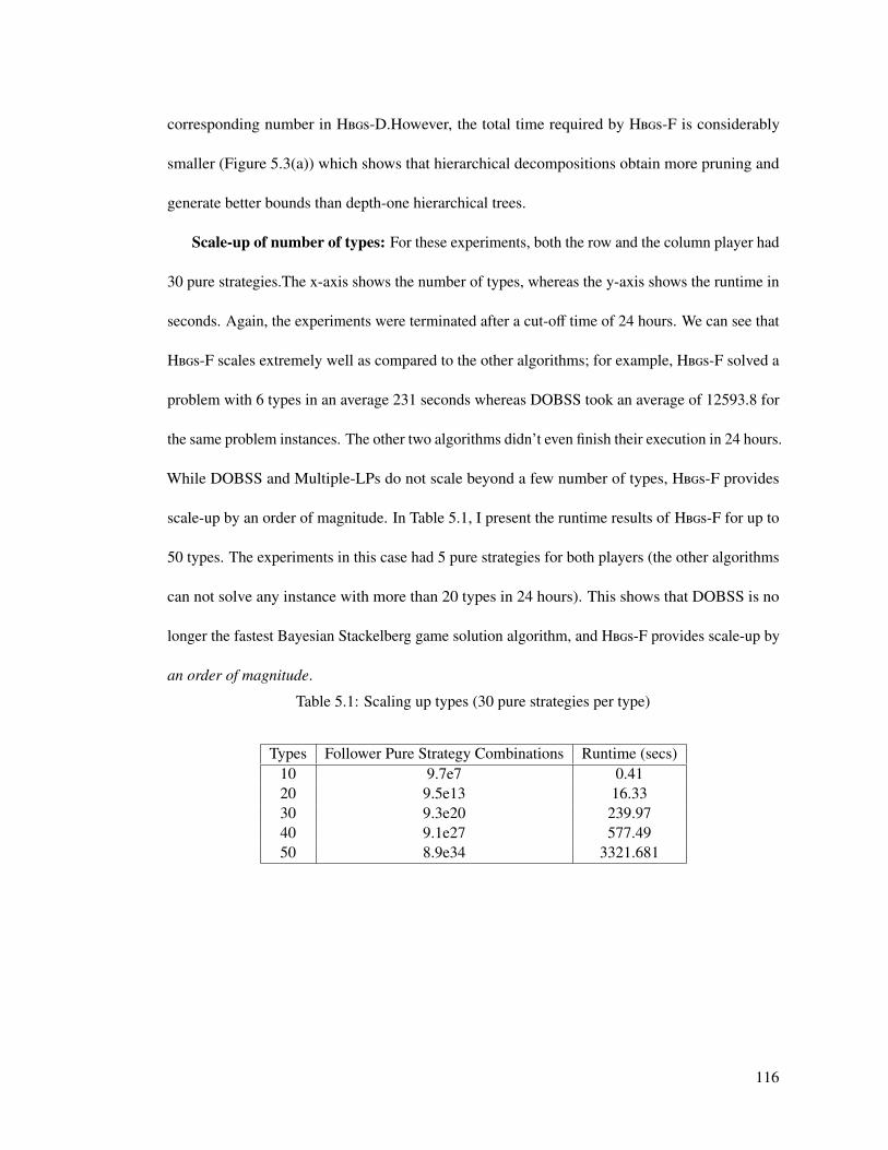
corresponding number in Hbgs-D.However, the total time required by Hbgs-F is considerably

smaller (Figure 5.3(a)) which shows that hierarchical decompositions obtain more pruning and

generate better bounds than depth-one hierarchical trees.

Scale-up of number of types: For these experiments, both the row and the column player had

30 pure strategies.The x-axis shows the number of types, whereas the y-axis shows the runtime in

seconds. Again, the experiments were terminated after a cut-off time of 24 hours. We can see that

Hbgs-F scales extremely well as compared to the other algorithms; for example, Hbgs-F solved a

problem with 6 types in an average 231 seconds whereas DOBSS took an average of 12593.8 for

the same problem instances. The other two algorithms didn’t even finish their execution in 24 hours.

While DOBSS and Multiple-LPs do not scale beyond a few number of types, Hbgs-F provides

scale-up by an order of magnitude. In Table 5.1, I present the runtime results of Hbgs-F for up to

50 types. The experiments in this case had 5 pure strategies for both players (the other algorithms

can not solve any instance with more than 20 types in 24 hours). This shows that DOBSS is no

longer the fastest Bayesian Stackelberg game solution algorithm, and Hbgs-F provides scale-up by

an order of magnitude.

Table 5.1: Scaling up types (30 pure strategies per type)

Types Follower Pure Strategy Combinations Runtime (secs)10 9.7e7 0.4120 9.5e13 16.3330 9.3e20 239.9740 9.1e27 577.4950 8.9e34 3321.681

116

5.1.3.2 Approximations

This section discusses the performance scale-ups that can be achieved when the algorithm was

allowed to return approximation solutions. Three parameter settings of approximations were

allowed: 1 unit, 5 unit and 10 units5. The approximations were tried on Hbgs-F (with fully

branched binary trees) since that prior experiments had shown it to be the fastest algorithm.

The number of types was fixed to 6 and the number of pure strategies was varied for the results

shown in Figure 5.4(a). The number of targets here is shown on the x-axis, whereas the y-axis

shows the runtime in seconds. Similarly, Figure 5.4(b) shows the results when the number of types

was increased while fixing the strategy space to 50 pure strategies for the leader and all follower

types. These figures show that the approximation variants of Hbgs scale significantly better. For

example, while Hbgs-F took 43,727 seconds to solve a problem instance with 50 pure strategies

and 6 types, the 1,5 and 10 unit approximations were able to solve the same problem in 10639,

3131 and 2409 seconds respectively, which is up to 18 times faster.

I also analyzed the difference in solution quality when the approximations were allowed, which

is shown in Figure 5.4(c). The y-axis shows the percentage error in the actual solution quality of

the approximate solution while the x-axis shows the number of targets. Lower bar implies lower

error. For example, the maximum error in all settings for Hbgs with an allowed approximation of

five units was less than two percent. These results show that allowing for approximate solutions

can dramatically increase the scalability of the algorithms without significant loss in the solution

quality.

5The maximum reward in the matrix was 100 units, and these were chosen as 1%, 5% and 10% of the maximumpossible payoff.

117

0.00  

10000.00  

20000.00  

30000.00  

40000.00  

50000.00  

10   20   30   40   50  

Run,

me  (secs)  

Pure  Strategies  

HBGS  Approx  1  Approx  5  Approx  10  

(a) Scaling Up Targets

0.00

10000.00

20000.00

30000.00

40000.00

50000.00

4   5   6  

Run(

me  (secs)  

Types  

HBGS  

Approx  1  

Approx  5  

Approx  10  

(b) Scaling Up Types

0  

1  

2  

3  

4  

5  

1   2   3   4   5  Percen

tage  Error  

Targets  

Approx  1  

Approx  5  

Approx  10  

(c) Solution Quality

Figure 5.4: This plot shows the comparisons of Hbgs and its approximation variants.

5.2 Solving Bayesian-SPARS Problem Instances

I now present Hierarchical Bayesian Solver for Security games with Arbitrary schedules, or Hbsa,

an algorithm that computes solutions to Bayesian-SPARS instances. First, I extend the basic

Aspen problem formulation to include multiple attacker types so it can be applied to instances

of Bayesian-SPARS. Hbsa uses the same hierarchical framework as described above in Hbgs,

however, it uses my new Bayesian-Aspen formulation to solve each node in the attacker action

tree. I now describe Bayesian-Aspen approach in more detail.

5.2.1 Bayesian-Aspen

Bayesian-Aspen computes solutions to instances of the Bayesian-SPARS problem. It uses column

generation to evaluate leaves of the attacker action tree from Figure 5.1, and I first describe this

procedure. Then I describe the methods for using branching and bounding heuristics to reduce the

overall computation done on the tree.

118

5.2.1.1 Bayesian-Aspen Column Generation

The column generation procedure used in Bayesian-Aspen is similar to methods used in Aspen,

as described in Section 3.1.1. The primary differences are extensions to the master problem

formulation to include multiple attacker types, and updated computations for the reduced cost

calculations used in the slave network flow problem.

Master Problem for Bayesian-Aspen: The defender and the adversary optimization con-

straints from Aspen need to be extended over all adversary types, in accordance with the definition

of SSE. The master problem, given in Equations (5.4) to (5.8), solves for the probability vector x

that maximizes the defender reward.6 Equations (5.5) and (5.6) enforce the SSE conditions for the

defender and adversary of each type, such that the attacker of each type chooses his best-responses.

Additionally, the chosen defender strategy is such that maximizes the defender’s payoff, as given

by the objective in Equation (5.4). Here, dλ refers to the expected utility of the defender when

the defender has committed to the mixed strategy x and the attacker of type λ has chosen the

best response aλ. The defender expected utility for protecting target t against adversary type λ

is given by the tth component of the column vector DλPx + Uλ,uΘ

(the adversary payoff is defined

6Just like in Aspen, the actual algorithm minimizes the negative of the defender reward for correctness of reducedcost computation, and I show maximization of defender reward only for expository purposes.

119

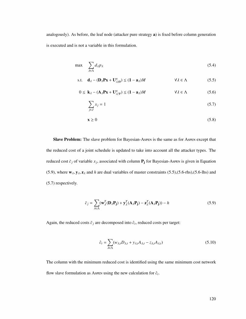
analogously). As before, the leaf node (attacker pure strategy a) is fixed before column generation

is executed and is not a variable in this formulation.

max∑λ∈Λ

dλpλ (5.4)

s.t. dλ − (DλPx + Uuλ,Θ) ≤ (1 − aλ)M ∀λ ∈ Λ (5.5)

0 ≤ kλ − (AλPx + Uuλ,Ψ) ≤ (1 − aλ)M ∀λ ∈ Λ (5.6)∑

j∈J

x j = 1 (5.7)

x ≥ 0 (5.8)

Slave Problem: The slave problem for Bayesian-Aspen is the same as for Aspen except that

the reduced cost of a joint schedule is updated to take into account all the attacker types. The

reduced cost c j of variable x j, associated with column Pj for Bayesian-Aspen is given in Equation

(5.9), where wλ, yλ, zλ and h are dual variables of master constraints (5.5),(5.6-rhs),(5.6-lhs) and

(5.7) respectively.

c j =∑λ∈Λ

(wTλ (DλPj) + yT

λ (AλPj) − zTλ (AλPj)) − h (5.9)

Again, the reduced costs c j are decomposed into ct, reduced costs per target:

ct =∑λ∈Λ

(wλ,tDλ,t + yλ,tAλ,t − zλ,tAλ,t) (5.10)

The column with the minimum reduced cost is identified using the same minimum cost network

flow slave formulation as Aspen using the new calculation for ct.

120

5.2.1.2 Improving Branching and Bounds

Aspen used the ORIGAMI heuristic to arrange the leaves representing the attacker pure strategies

for a SPARS problem instance, as shown in Figure 3.1. ORIGAMI-S is designed only for security

games with one attacker type, and hence is not directly applicable to Bayesian-Aspen. However,

we can adapt the method for Bayesian-Aspen by solving ORIGAMI-S for each attacker type λ

independently and then using the weighted combination of the solutions as branch and bound

heuristics. The solutions are weighted by the probability pλ of facing the attacker type λ. For

example, if the ORIGAMI-S solution for type 1 provides a defender upper bound of B(t12) for

target t2, and the ORIGAMI-S solution to type 2 provides a defender upper bound of B(t21) for

target t1, then the upper bound used by Bayesian-Aspen for the leaf [2, 1] in Figure 5.1 would be

B(t12)p1 + B(t2

1)p2, where p1 and p2 are the probabilities for attacker type 1 and 2 respectively.

This upper bound is valid because if the defender cannot perform better than B(tλi ) against each

attacker type λ independently, then it cannot perform better than B(tλi )pλ when it is facing the type

λ with probability pλ. Bayesian-Aspen computes the upper bound for all the leaves, sorts them in

decreasing order and then uses column generation to compute the exact solution for each leaf until

(i) the exact solution for all the leaves has been computed, or (ii) a solution has been obtained that

is better than the upper bound for all remaining leaves.

I now introduce Hbsa that builds on Bayesian-Aspen and further reduces the number of leaves

(refer Figure 5.1) that must be evaluated. This section will also clarify the use of Bayesian-Aspen

in Hbsa. I will then provide an experimental comparison of Hbsa and Bayesian-Aspen with

ORIGAMI-S in the following experimental results section.

121

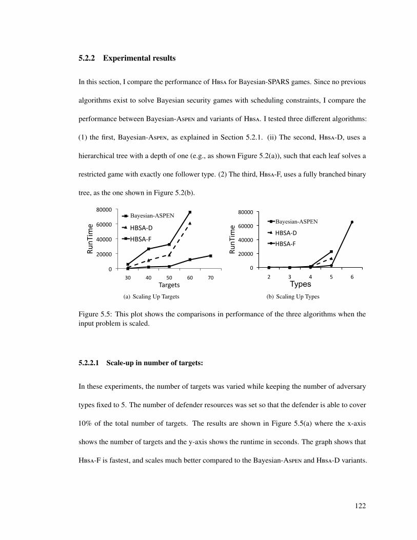
5.2.2 Experimental results

In this section, I compare the performance of Hbsa for Bayesian-SPARS games. Since no previous

algorithms exist to solve Bayesian security games with scheduling constraints, I compare the

performance between Bayesian-Aspen and variants of Hbsa. I tested three different algorithms:

(1) the first, Bayesian-Aspen, as explained in Section 5.2.1. (ii) The second, Hbsa-D, uses a

hierarchical tree with a depth of one (e.g., as shown Figure 5.2(a)), such that each leaf solves a

restricted game with exactly one follower type. (2) The third, Hbsa-F, uses a fully branched binary

tree, as the one shown in Figure 5.2(b).

0"

20000"

40000"

60000"

80000"

30" 40" 50" 60" 70"

RunTim

e"

Targets"

HBSA:O"

HBSA:D"

HBSA:F"

Bayesian-ASPEN

(a) Scaling Up Targets

0"

20000"

40000"

60000"

80000"

2" 3" 4" 5" 6"

RunTim

e"

Types

HBSA4O"

HBSA4D"

HBSA4F"

Bayesian-ASPEN

(b) Scaling Up Types

Figure 5.5: This plot shows the comparisons in performance of the three algorithms when theinput problem is scaled.

5.2.2.1 Scale-up in number of targets:

In these experiments, the number of targets was varied while keeping the number of adversary

types fixed to 5. The number of defender resources was set so that the defender is able to cover

10% of the total number of targets. The results are shown in Figure 5.5(a) where the x-axis

shows the number of targets and the y-axis shows the runtime in seconds. The graph shows that

Hbsa-F is fastest, and scales much better compared to the Bayesian-Aspen and Hbsa-D variants.

122

The simulations were terminated if they didn’t finish in 24 hours. For example, Hbsa-D and

Bayesian-Aspen did not finish in 24 hours for the case with 70 targets, while Hbsa-F was able to

solve the problem instance in less than 5 hours.

5.2.2.2 Scale-up in number of types:

These experiments varied the number of types, while keeping the number of targets fixed to 50.

The number of resources was set to 5, so as to cover 10% of the total number of targets. The x-axis

shows the number of types whereas the y-axis shows the runtime in seconds. The graph again

shows that Hbsa-F is the fastest algorithm. Again, the cut-off time for the experiments was 24

hours, and for example, Hbsa-D and Bayesian-Aspen could not solve for 6 types in 24 hours.

5.2.2.3 Effects of using different hierarchies

The objective of these experiments is to further explore the impact of using different tree arrange-

ments in the runtime performance of Hbsa. While my previous experiments showed that the full

binary tree arrangement was better than using a depth-one arrangement, this experiment is designed

to investigate the trade-off between pre-processing and actual computation: a greater depth in

the hierarchical tree implies more preprocessing but also better bounds, which are conflicting

factors contributing to the total runtime. Specifically, I explore the runtime performance of an

intermediate level tree, the depth-two tree. An example of a depth-two tree for 8 attacker types

is shown in Figure 5.6. I generate random Bayesian-SPARS instances with 8 attacker types and

compare the runtime performance of the depth-two tree with the full binary tree (depth-three for

8 attacker types). I do not show results for the depth-one tree since that took substantially more

(more than 5 hours for some instances) when the number of targets was more than 10.

123

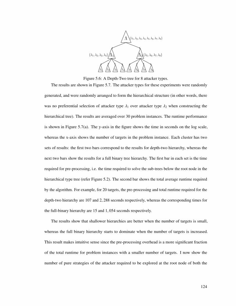
�1 �2 �3 �4 �5 �6 �7 �8

⇤

⇤1 ⇤2{�1,�2,�3,�4}

{�1,�2,�3,�4,�5,�6,�7,�8}

{�5,�6,�7,�8}

Figure 5.6: A Depth-Two tree for 8 attacker types.

The results are shown in Figure 5.7. The attacker types for these experiments were randomly

generated, and were randomly arranged to form the hierarchical structure (in other words, there

was no preferential selection of attacker type λ1 over attacker type λ2 when constructing the

hierarchical tree). The results are averaged over 30 problem instances. The runtime performance

is shown in Figure 5.7(a). The y-axis in the figure shows the time in seconds on the log scale,

whereas the x-axis shows the number of targets in the problem instance. Each cluster has two

sets of results: the first two bars correspond to the results for depth-two hierarchy, whereas the

next two bars show the results for a full binary tree hierarchy. The first bar in each set is the time

required for pre-processing, i.e. the time required to solve the sub-trees below the root node in the

hierarchical type tree (refer Figure 5.2). The second bar shows the total average runtime required

by the algorithm. For example, for 20 targets, the pre-processing and total runtime required for the

depth-two hierarchy are 107 and 2, 288 seconds respectively, whereas the corresponding times for

the full-binary hierarchy are 15 and 1, 054 seconds respectively.

The results show that shallower hierarchies are better when the number of targets is small,

whereas the full binary hierarchy starts to dominate when the number of targets is increased.

This result makes intuitive sense since the pre-processing overhead is a more significant fraction

of the total runtime for problem instances with a smaller number of targets. I now show the

number of pure strategies of the attacker required to be explored at the root node of both the

124

depth-two and full binary hierarchical type trees (refer (Figure 5.2) in Figure 5.7(b). Remember

that the number of pure strategies evaluated refers to the number of leaves explored in the tree

representing the attacker’s pure strategies (refer Figure 5.1), and that this directly corresponds

to the amount of computation required after the pre-processing has been completed. The y-axis

of Figure 5.7(b) shows the number of pure strategies evaluated for the attacker, whereas the

x-axis shows the number of targets. For example, the number of pure strategies expanded by the

depth-two hierarchy for 20 targets is 184, 763 whereas for the full binary hierarchy is 88, 422.

Similarly, for 15 targets, the number of pure strategies expanded by the depth-two hierarchy for

20 targets is 51, 096 whereas for the full binary hierarchy is 46, 108. Thus, in combination with

Figure 5.7(a), the experiment shows (i) the number of pure strategies evaluated for full binary

hierarchy is always no greater than the pure strategies evaluated for the depth-two hierarchy (the

difference in number of pure strategies evaluated is statistically significant only for 15 and 20

targets in Figure 5.7(b)), and (ii) the depth-two hierarchy is faster for lesser number of targets (for

5, 10 and 15 targets in Figure 5.7(a)) and slower for 20 targets. The results confirms that there

exists a trade-off in the choice of the hierarchy: deeper trees are faster only when the number of

targets are large otherwise the overhead of pre-processing overwhelms the total runtime required

to solve the problem.

5.2.2.4 Different arrangement of types in Hbsa

The objective of these experiments is to identify the impact of the distribution of types in the

runtime performance of Hbsa as the number of targets is increased. I test two arrangements in

these experiments: one that puts similar types in the same sub-tree whereas other which combines

dissimilar types. The optimal coverage vectors cλ = Px are computed per type λ by solving

125

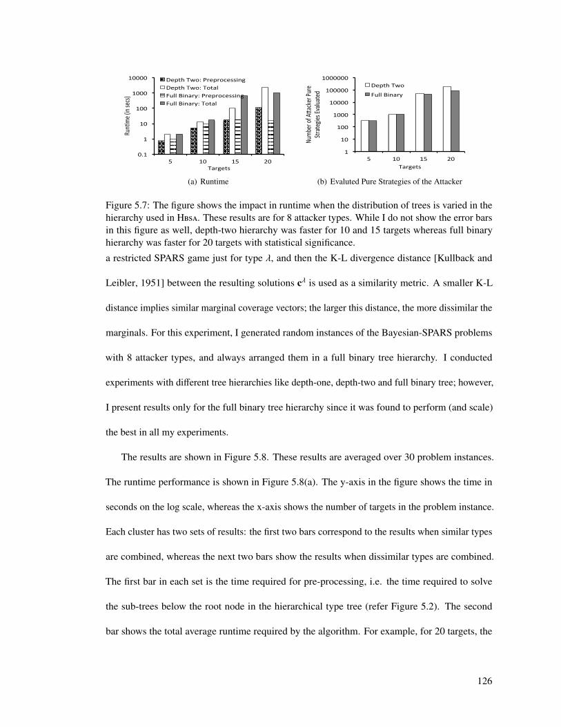
0.1  

1  

10  

100  

1000  

10000  

5   10   15   20  

Run*

me  (in

 secs)

 

Targets  

Depth  Two:  Preprocessing  Depth  Two:  Total  Full  Binary:  Preprocessing  Full  Binary:  Total  

(a) Runtime

1  

10  

100  

1000  

10000  

100000  

1000000  

5   10   15   20  

Numb

er  of

 A/acker  P

ure  

Strate

gies  E

valua

ted  

Targets  

Depth  Two  

Full  Binary  

(b) Evaluted Pure Strategies of the Attacker

Figure 5.7: The figure shows the impact in runtime when the distribution of trees is varied in thehierarchy used in Hbsa. These results are for 8 attacker types. While I do not show the error barsin this figure as well, depth-two hierarchy was faster for 10 and 15 targets whereas full binaryhierarchy was faster for 20 targets with statistical significance.

a restricted SPARS game just for type λ, and then the K-L divergence distance [Kullback and

Leibler, 1951] between the resulting solutions cλ is used as a similarity metric. A smaller K-L

distance implies similar marginal coverage vectors; the larger this distance, the more dissimilar the

marginals. For this experiment, I generated random instances of the Bayesian-SPARS problems

with 8 attacker types, and always arranged them in a full binary tree hierarchy. I conducted

experiments with different tree hierarchies like depth-one, depth-two and full binary tree; however,

I present results only for the full binary tree hierarchy since it was found to perform (and scale)

the best in all my experiments.

The results are shown in Figure 5.8. These results are averaged over 30 problem instances.

The runtime performance is shown in Figure 5.8(a). The y-axis in the figure shows the time in

seconds on the log scale, whereas the x-axis shows the number of targets in the problem instance.

Each cluster has two sets of results: the first two bars correspond to the results when similar types

are combined, whereas the next two bars show the results when dissimilar types are combined.

The first bar in each set is the time required for pre-processing, i.e. the time required to solve

the sub-trees below the root node in the hierarchical type tree (refer Figure 5.2). The second

bar shows the total average runtime required by the algorithm. For example, for 20 targets, the

126

pre-processing and total runtime required for the ‘similar’ arrangement are 12 and 1, 028 seconds

respectively, whereas the corresponding times for the ‘dissimilar’ arrangement are 21 and 2, 578

seconds, respectively.

The results show that combining similar types is always more helpful than combining dissimilar

types. This result makes intuitive sense since combining similar types is expected to generate

tighter bounds (since the defender is better able to optimize against two similar opponents),

resulting in more pruning at every subsequent parent node. To test this hypothesis, I also plot

the number of pure strategies of the attacker (refer Figure 5.1) that are expanded at the root node

of the hierarchical type tree (refer (Figure 5.2). Like in the previous experiment, the number of

pure strategies of the attacker represents the number of leaves from Figure 5.1 that are expanded

by the Hbsa algorithm after the pre-processing has been completed. These results are shown in

Figure 5.8(b). The y-axis shows the number of pure strategies evaluated for the attacker, whereas

the x-axis shows the number of targets. For example, the number of pure strategies expanded

by the ‘similar’ arrangement for 20 targets is 80, 781 whereas for the ‘dissimilar’ arrangement is

160, 502 respectively. The results confirm my hypothesis that combining similar types results in

fewer pure strategies of the attacker being evaluated.

5.3 Bayesian SPPC Domain

In this section, I present the solution methodology for solving the Bayesian extension of the SPPC

domain. Again, the defender does not know the type of the attacker she would be facing, however,

the defender does know a prior probability of facing each type. The attacker knows his type as

well the defender strategy, and then computes his best response.

127

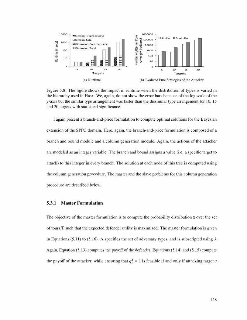
1  

10  

100  

1000  

10000  

5   10   15   20  

Run)

me  (in

 secs)

 

Targets  

Similar:  Preprocessing  

Similar:  Total  

Dissimilar:  Preprocessing  

Dissimilar:  Total  

(a) Runtime

1  

10  

100  

1000  

10000  

100000  

1000000  

5   10   15   20  

Numb

er  of

 A/acker  P

ure  

Strate

gies  E

valua

ted  

Targets  

Similar   Dissimilar  

(b) Evaluted Pure Strategies of the Attacker

Figure 5.8: The figure shows the impact in runtime when the distribution of types is varied inthe hierarchy used in Hbsa. We, again, do not show the error bars because of the log scale of they-axis but the similar type arrangement was faster than the dissimilar type arrangement for 10, 15and 20 targets with statistical significance.

I again present a branch-and-price formulation to compute optimal solutions for the Bayesian

extension of the SPPC domain. Here, again, the branch-and-price formulation is composed of a

branch and bound module and a column generation module. Again, the actions of the attacker

are modeled as an integer variable. The branch and bound assigns a value (i.e. a specific target to

attack) to this integer in every branch. The solution at each node of this tree is computed using

the column generation procedure. The master and the slave problems for this column generation

procedure are described below.

5.3.1 Master Formulation

The objective of the master formulation is to compute the probability distribution x over the set

of tours T such that the expected defender utility is maximized. The master formulation is given

in Equations (5.11) to (5.16). Λ specifies the set of adversary types, and is subscripted using λ.

Again, Equation (5.13) computes the payoff of the defender. Equations (5.14) and (5.15) compute

the payoff of the attacker, while ensuring that qλs = 1 is feasible if and only if attacking target s

128

is the best response of the attacker of type λ. Equations (5.12) and (5.16) ensure that x is a valid

probability distribution.

minx,d,q−

∑λ∈Λ

dλ (5.11)

s.t.∑t∈T

xt ≤ 1 (5.12)

dλ −∑t∈T

xtzst(τλs + Rλs ) + Mqλs ≤ M − Rλs (5.13)

−kλ −∑t∈T

xtzst(Pλ + Rλs ) + Rλs ≤ 0 (5.14)

kλ +∑t∈T

xtzst(Pλ + Rλs ) + Mqλs − Rλs ≤ M (5.15)

xt ∈ [0, 1] (5.16)

5.3.2 Slave

The objective of the slave formulation is the compute the next best tour to add to the set of tours T.

This is again done using a minimum cost integer network flow formulation. The network flow graph

is constructed in the same way as before. The updated reduced costs for this variant of the domain

are computed using the same standard techniques and are given in the Equation (5.17). Here, wλ,

yλ, vλ and h represent the duals of Equations (5.13), (5.14), (5.15) and (5.12) respectively.

ct =∑λ∈Λ

∑s∈S

(wλs (τλs + Rλs ) + (vλs − yλs )(Pλs + Rλs ))zst − h (5.17)

129

This reduced cost of a tour ct is again decomposed into reduced costs per target in the following

manner:

ct =∑

s∈S cszst − h (5.18)

cs =∑λ∈Λ(wλ

s (τλs + Rλs ) + (vλs − yλs )(Pλs + Rλs )) (5.19)

These reduced costs per target, cs, are then put as the costs on the links of the minimum cost

network flow formulation.

The results of the runtime of this domain are presented with detailed analysis in Chapter 6.

130

Chapter 6: d:s and Phase Transition

Software security assistants built on the framework of Stackelberg security games [Kiekintveld

et al., 2009] have been deployed by a variety of real-world security agencies. For example,

ARMOR [Jain et al., 2010c] has been in use by the police at Los Angeles International Airport

since 2007. Similarly, IRIS [Jain et al., 2010c] and PROTECT [An et al., 2011] have been in use

by the US Federal Air Marshals Service and the US Coast Guard since 2009 and 2011 respectively.

Many different algorithms have been proposed for computing solutions to such problems [Conitzer

and Sandholm, 2006; Paruchuri et al., 2008b; Gatti, 2008; Kiekintveld et al., 2009; Jain et al.,

2010b; Dickerson et al., 2010b; Letchford and Vorobeychik, 2011; Bosansky et al., 2011] with

a focus on scalability to enable the application of these models to newer and more complex

real-world domains.

In this chapter, I investigate what properties of Stackelberg security game instances make

them hard to solve in practice, across different input sizes and different security domains. I show

that this question can be answered using the novel concept of the deployment-to-saturation (d:s)

ratio. This ratio, which we denote d:s, is defined as the number of deployed defender resources

divided by the number of resources beyond which additional deployments would not provide any

benefit to the defender. I show that the hardest computational instances arise when this ratio is

131

0.5, independent of the domain representation, model and solver. Specifically, I consider three

different classes of security domains, eight different MIP algorithms (including two algorithms

actually deployed in practice), five different underlying MIP solvers, two different variations on

the Stackelberg equilibrium concept, and a variety of domain sizes and conditions.

I identify two important implications of my findings. First, new algorithms should be compared

on the hardest problem instances; I show that most previous research has compared the runtime

performance of algorithms only at low d:s ratios, where problems are comparatively easy. Second,

I argue that this computationally hard region is the point where optimization offers the greatest

benefit to security agencies, implying that problems in this region deserve increased attention from

researchers.

Finally, I leverage the concept of phase transitions to better understand this algorithm-

independent, computationally hard region. This approach to understanding algorithm-independent

structural properties was pioneered by [Cheeseman et al., 1991] and [Mitchell et al., 1992]. They

showed that the probability that a uniform-random 3-SAT instance will be satisfiable exhibits a

phase transition when the number of variables is fixed and the number of clauses crosses roughly

4.3 times the number of variables, which corresponds to the point where the probability that the

instance will be solvable crosses 0.5. Phase transitions have also been used to understand the

computational impact of problem structure in optimization problems, such as MAX-SAT [Slaney

and Walsh, 2002] and TSP [Gent and Walsh, 1996; Frank et al., 1998]. The approach taken in

this work is to identify a phase transition in the decision version of the optimization problem (i.e.,

asking whether or not a solution exists with a given objective function value). I show that security

games exhibit a phase transition at 0.5 for random Stackelberg security game instances, and that

this phase transition corresponds to the computationally hardest instances at the d:s ratio of 0.5.

132

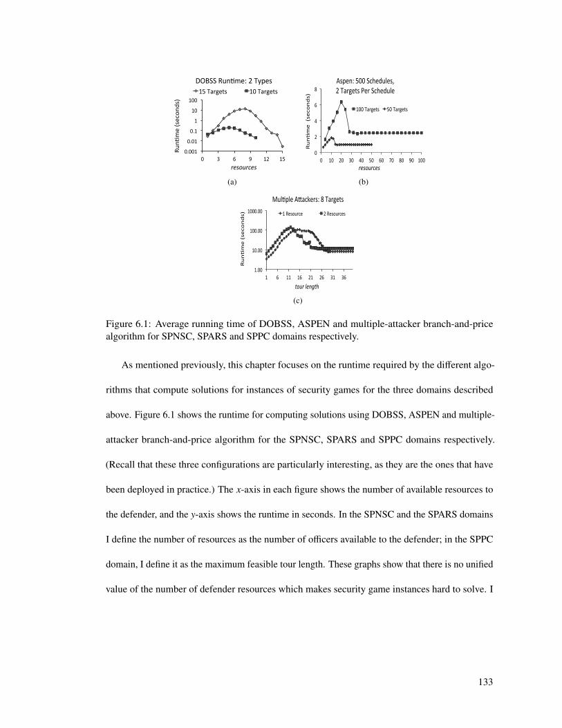
0.001  

0.01  

0.1  

1  

10  

100  

0   3   6   9   12   15  

Run-

me  (secon

ds)    

resources  

DOBSS  Run-me:  2  Types  15  Targets   10  Targets  

(a)

0  

2  

4  

6  

8  

0   10   20   30   40   50   60   70   80   90   100  

Run/me    (seconds)  

resources  

Aspen:  500  Schedules,    2  Targets  Per  Schedule  

100  Targets   50  Targets  

(b)

1.00  

10.00  

100.00  

1000.00  

1   6   11   16   21   26   31   36  

Run+me  (seconds)  

tour  length  

Mul+ple  A8ackers:  8  Targets  

1  Resource   2  Resources  

(c)

Figure 6.1: Average running time of DOBSS, ASPEN and multiple-attacker branch-and-pricealgorithm for SPNSC, SPARS and SPPC domains respectively.

As mentioned previously, this chapter focuses on the runtime required by the different algo-

rithms that compute solutions for instances of security games for the three domains described

above. Figure 6.1 shows the runtime for computing solutions using DOBSS, ASPEN and multiple-

attacker branch-and-price algorithm for the SPNSC, SPARS and SPPC domains respectively.

(Recall that these three configurations are particularly interesting, as they are the ones that have

been deployed in practice.) The x-axis in each figure shows the number of available resources to

the defender, and the y-axis shows the runtime in seconds. In the SPNSC and the SPARS domains

I define the number of resources as the number of officers available to the defender; in the SPPC

domain, I define it as the maximum feasible tour length. These graphs show that there is no unified

value of the number of defender resources which makes security game instances hard to solve. I

133

also tried normalizing the number of resources by the number of targets, however, I found similar

inconsistencies across different domains even with that normalization.

6.1 Deployment to Saturation Ratio

I now propose the novel concept of the deployment-to-saturation (d:s) ratio, a concept that uni-

fies the domain independent properties of problem instances across different security domains.

Specifically, I consider the three security domains introduced before, eight different MIP algo-

rithms (including two deployed algorithms), five different underlying MIP solvers, two different

equilibrium concepts in Stackelberg security games, and a variety of domain sizes and conditions.

I show experimentally that the hardest problem instances occur when the dts ratio is about 0.5.

(Specifically, in my experiments, the hardest problem instances occurred at the d:s ratios between

0.48 and 0.54. However, because of discretization, I was not able to test all d:s ratios in all

domains. Without exception, the hardest value was the feasible value closest to 0.5. This fact, in

combination with my phase transition arguments presented at the end of the chapter, lead me to

conclude that the hardest region is precisely d:s = 0.5.)

More specifically, the deployment-to-saturation (d:s) ratio is defined in terms of defender

resources, a concept whose precise definition differs from one domain to another. Given this

definition, deployment denotes the number of defender resources available to be allocated, and

saturation denotes the minimum number of defender resources such that the addition of further

resources beyond this point yields no increase in the defender’s expected utility. For the SPNSC

and the SPARS domain, deployment denotes the number of available security personnel, whereas

saturation refers to the minimum number of officers required to cover all targets with a probability

134

of 1. For the SPPC domain, deployment denotes the maximum feasible tour length, while saturation

denotes the minimum tour length required by the team of defender resources such that the team

can tour all the targets with a probability of 1.

I now present results for all the three security domains. All the results shown below are

averaged over 100 samples, and were collected on a machine with a 2.7GHz Intel Core i7

processor and 8GB main memory. In all graphs, the x-axis shows the d:s ratio and the y-axis shows

the runtime in CPU-seconds. Experiments were conducted using CPLEX 12.2 unless otherwise

noted.

6.1.1 SPNSC Domain

For this domain, I considered both the general-sum and security game compact representations.

6.1.1.1 General sum representation.

I conducted experiments varying the algorithm, number of attacker types and number of targets.

The results for the general sum representation are plotted in Figures 6.2(a), 6.2(b) and 6.2(c). The

payoffs for the two players were selected uniformly at random: the payoffs for success and failure

were selected from the ranges [1, 10] and [−10,−1] respectively.

Figure 6.2(a) shows that the runtime required by all three algorithms (MultipleLPs, DOBSS

and HBGS) peaks at d:s = 0.53. (While I would like to have observed peaks at d:s = 0.5 in all

of my experiments, I typically observed values that were slightly different. The explanation that

might come first to mind is variance due to having measured an insufficient number of samples.

However, there is also a more critical issue: because the numbers of resources and targets are

discrete, I was not able to measure every d:s value. Here, 8 resources and 15 targets corresponded

135

0.001  

0.01  

0.1  

1  

10  

100  

0   0.2   0.4   0.6   0.8   1  

Run

,me  (secon

ds)    

d:s  ra,o  

Varia,on  in  Algorithms:    2  Types,  15  Targets  

Mul,ple  LPs   DOBSS   HBGS    

(a)

0.001  

0.01  

0.1  

1  

10  

100  

0   0.2   0.4   0.6   0.8   1  

Run,

me  (secon

ds)    

d:s  ra,o  

DOBSS  Run,me:  2  Types  10  Targets   15  Targets  

(b)

0.001  

0.01  

0.1  

1  

10  

0   0.2   0.4   0.6   0.8   1  

Run,

me  (secon

ds)    

d:s  ra,o  

DOBSS  Run,me:  10  Targets  2  Types   3  Types  

(c)

0.001  0.01  0.1  1  10  

100  1000  

0.00   0.20   0.40   0.60   0.80   1.00  

Run,me  (seconds)    

d:s  ra,o  

Brass:  2  Types  

15  Targets   10  Targets  

(d)

0  

0.4  

0.8  

1.2  

1.6  

2  

0   0.2   0.4   0.6   0.8   1  Run,me  (seconds)  

d:s  ra,o  

Eraser  Run,me:  2  Types  50  Targets   75  Targets  

(e)

0  

0.5  

1  

1.5  

2  

0   0.2   0.4   0.6   0.8   1  

Run-

me  (secon

ds)  

d:s  ra-o  

Varia-on  in  Solu-on  Mechanism:    2  Types,    50  Targets  

CPLEX:  Primal  Simplex   CPLEX:  Dual  Simplex  CPLEX:  Network  Simplex   CPLEX:  Barrier  GLPK  Simplex  

(f)

Figure 6.2: Average runtime of computing the optimal solution for a SPNSC problem instance.The vertical dotted line shows d:s = 0.5.

to d:s = 0.53.) This set of experiments considered 2 attacker types and 15 targets. Moreover, all

the three algorithms required the maximum runtime when the d:s ratio was 0.53. For example,

MultipleLPs required 27.9 seconds to compute the optimal solution. This experiment shows that

computation is hardest for the SPNSC problem instances when the d:s ratio is about 0.5.

The next two experiments study runtime variation when the number of targets and the number

of types in the domain vary. Figure 6.2(b) varies the number of targets in the domain from 10 to

136

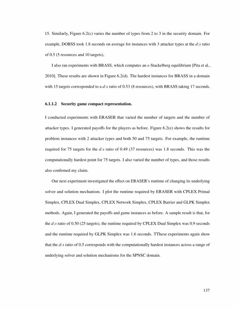
15. Similarly, Figure 6.2(c) varies the number of types from 2 to 3 in the security domain. For

example, DOBSS took 1.8 seconds on average for instances with 3 attacker types at the d:s ratio

of 0.5 (5 resources and 10 targets),

I also ran experiments with BRASS, which computes an ε-Stackelberg equilibrium [Pita et al.,

2010]. These results are shown in Figure 6.2(d). The hardest instances for BRASS in a domain

with 15 targets corresponded to a d:s ratio of 0.53 (8 resources), with BRASS taking 17 seconds.

6.1.1.2 Security game compact representation.

I conducted experiments with ERASER that varied the number of targets and the number of

attacker types. I generated payoffs for the players as before. Figure 6.2(e) shows the results for

problem instances with 2 attacker types and both 50 and 75 targets. For example, the runtime

required for 75 targets for the d:s ratio of 0.49 (37 resources) was 1.8 seconds. This was the

computationally hardest point for 75 targets. I also varied the number of types, and those results

also confirmed my claim.

Our next experiment investigated the effect on ERASER’s runtime of changing its underlying

solver and solution mechanism. I plot the runtime required by ERASER with CPLEX Primal

Simplex, CPLEX Dual Simplex, CPLEX Network Simplex, CPLEX Barrier and GLPK Simplex

methods. Again, I generated the payoffs and game instances as before. A sample result is that, for

the d:s ratio of 0.50 (25 targets), the runtime required by CPLEX Dual Simplex was 0.9 seconds

and the runtime required by GLPK Simplex was 1.6 seconds. TThese experiments again show

that the d:s ratio of 0.5 corresponds with the computationally hardest instances across a range of

underlying solver and solution mechanisms for the SPNSC domain.

137

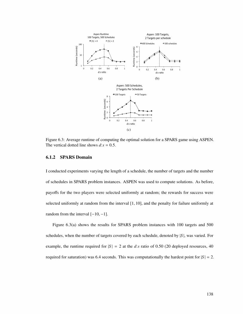
1  

10  

100  

0   0.2   0.4   0.6   0.8   1  

Run,

me  (secon

ds)  

 

d:s  ra,o  

Aspen  Run,me  100  Targets,  500  Schedules  

|S|  =  4   |S|  =  2  

(a)

0  

2  

4  

6  

8  

0   0.2   0.4   0.6   0.8   1  

Run,

me  (secon

ds)  

d:s  ra,o  

Aspen:  100  Targets,    2  Targets  per  schedule  

400  Schedules   500  schedules  

(b)

0  

2  

4  

6  

8  

0   0.2   0.4   0.6   0.8   1  

Run,

me    (secon

ds)  

d:s  ra,o  

Aspen:  500  Schedules,    2  Targets  Per  Schedule  

100  Targets   50  Targets  

(c)

Figure 6.3: Average runtime of computing the optimal solution for a SPARS game using ASPEN.The vertical dotted line shows d:s = 0.5.

6.1.2 SPARS Domain

I conducted experiments varying the length of a schedule, the number of targets and the number

of schedules in SPARS problem instances. ASPEN was used to compute solutions. As before,

payoffs for the two players were selected uniformly at random; the rewards for success were

selected uniformly at random from the interval [1, 10], and the penalty for failure uniformly at

random from the interval [−10,−1].

Figure 6.3(a) shows the results for SPARS problem instances with 100 targets and 500

schedules, when the number of targets covered by each schedule, denoted by |S |, was varied. For

example, the runtime required for |S | = 2 at the d:s ratio of 0.50 (20 deployed resources, 40

required for saturation) was 6.4 seconds. This was computationally the hardest point for |S | = 2.

138

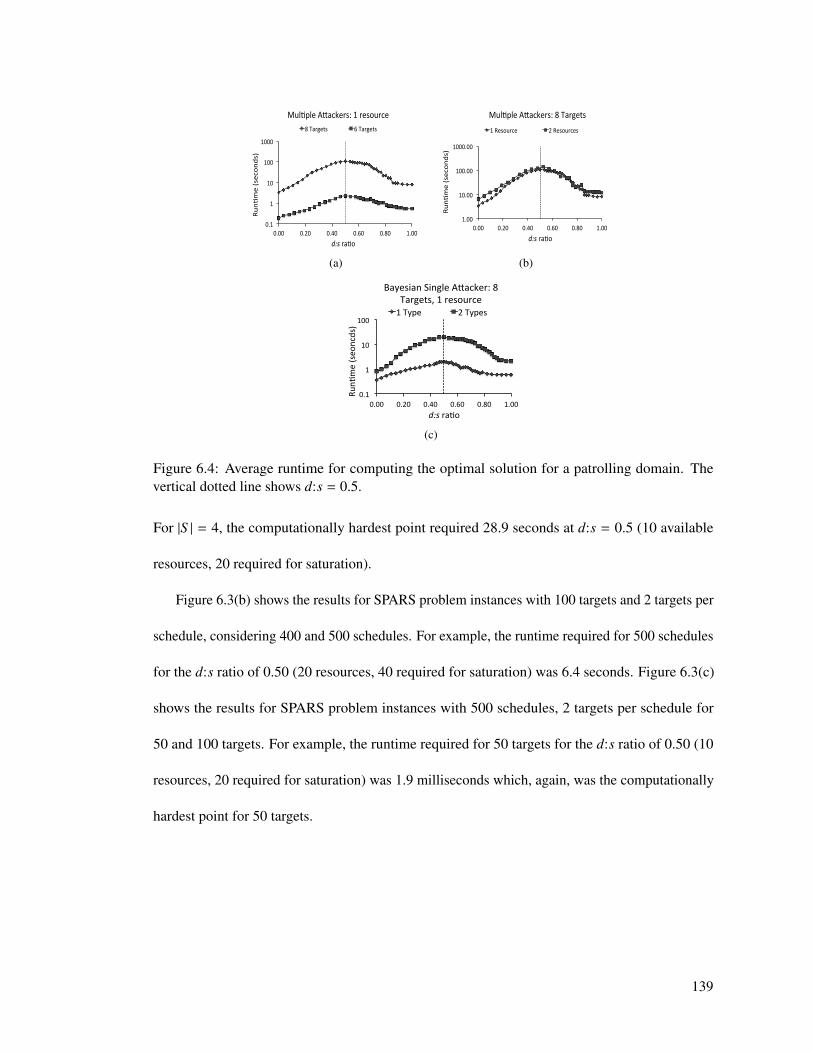
0.1  

1  

10  

100  

1000  

0.00   0.20   0.40   0.60   0.80   1.00  

Run

,me  (secon

ds)    

d:s  ra,o  

Mul,ple  A;ackers:  1  resource  8  Targets   6  Targets  

(a)

1.00  

10.00  

100.00  

1000.00  

0.00   0.20   0.40   0.60   0.80   1.00  

Run,

me  (secon

ds)  

d:s  ra,o  

Mul,ple  A;ackers:  8  Targets  1  Resource   2  Resources  

(b)

0.1  

1  

10  

100  

0.00   0.20   0.40   0.60   0.80   1.00  

Run,

me  (seo

ncds)  

d:s  ra,o  

Bayesian  Single  A>acker:  8  Targets,  1  resource  1  Type   2  Types  

(c)

Figure 6.4: Average runtime for computing the optimal solution for a patrolling domain. Thevertical dotted line shows d:s = 0.5.

For |S | = 4, the computationally hardest point required 28.9 seconds at d:s = 0.5 (10 available

resources, 20 required for saturation).

Figure 6.3(b) shows the results for SPARS problem instances with 100 targets and 2 targets per

schedule, considering 400 and 500 schedules. For example, the runtime required for 500 schedules

for the d:s ratio of 0.50 (20 resources, 40 required for saturation) was 6.4 seconds. Figure 6.3(c)

shows the results for SPARS problem instances with 500 schedules, 2 targets per schedule for

50 and 100 targets. For example, the runtime required for 50 targets for the d:s ratio of 0.50 (10

resources, 20 required for saturation) was 1.9 milliseconds which, again, was the computationally

hardest point for 50 targets.

139

6.1.3 SPPC Domain

I present results for both the multiple attacker and the Bayesian single attacker variants in Figure 6.4.

Figure 6.4(a) shows the results for the multiple attacker SPPC domain with 1 defender resource,

and with the number of targets varying from 6 to 8. For example, for the d:s ratio of 0.50, the

algorithm took 108.2 seconds to compute the optimal solution. Figure 6.4(b) shows the runtime

required to compute the optimal solution for the multple attacker SPPC domain with 8 targets. It

varies the number of defender resources from 1 to 2. For example, for the d:s ratio of 0.50, the

algorithm took 144.0 seconds to compute the optimal solution for 2 resources. This was again the

computationally hardest point.

Similarly, Figure 6.4(c) shows the runtime required for our branch-and-price based algorithm

to compute an optimal solution for the Bayesian single attacker SPPC domain with 8 targets and 1

defender resource, along with the probability p that the decision problem is solvable. It varies the

number of types from 1 to 2. For example, for the d:s ratio of 0.50, the algorithm took 2.0 seconds

to compute the optimal solution for 1 type.

6.2 Implications of the findings

I have provided evidence that the hardest random Stackelberg game instances occur at a

deployment-to-saturation ratio of 0.5. This finding has two key implications.

First, it is important to compare algorithms on hard problems. If random data is used to

test algorithms for security domains, it should be generated at a d:s ratio of 0.5. There has

indeed been a significant research effort focusing on the design of faster algorithms for security

domains. Random data has often been used; unfortunately, I find that it tends not to have come

140

from the d:s = 0.5 region. (Of course, the concept of a deployment-to-saturation ratio did not

previously exist; nevertheless, I can assess previous work in terms of the d:s ratio at which data was

generated.) For example, [Jain et al., 2011a] compared the performance of HBGS with DOBSS

and MultipleLPs, but they only compared d:s ratios between 0.10 and 0.20. Similarly, [Pita et al.,

2010] presented runtime comparisons between different algorithms, varying the number of attacker

types in the security domain; all experiments in this chapter were fixed at d:s = 0.30 (10 targets, 3

resources). [Jain et al., 2011b] showed scalability results for RUGGED, testing at d:s ratios of 0.10

and (mostly) 0.20. Runtime results have also been presented in other security settings [Dickerson

et al., 2010b; Vanek et al., 2011; Bosansky et al., 2011]; these algorithms compute defender

strategies for networked domains. Their experiments keep the number of resources fixed and

increase the size of the underlying network; however, none of these papers provides enough detail

about how instances were generated to allow us to accurately compute the d:s ratio.

To make it easier for future researchers to test their algorithms on hard problems, I have written

a benchmark generator for security games that generates instances from d:s = 0.5. This generator

is written in Java, and is available for download at http://teamcore.usc.edu/DTS. It allows

users to generate instances for all domains described above, as well as to compute solutions for all

the algorithms mentioned in this research. It also allows switching between GLPK and CPLEX.

Second, I observe that intermediate values of the d:s ratio, the computationally hard region, is

also the region where optimization is most valuable and hence where security officials are most

likely to seek help in optimizing their resource deployment. If the d:s ratio is large, there are

enough resources to protect almost all targets, and performing a rigorous optimization offers little

additional benefit. If d:s is small, there are not enough resources for optimized deployment to

have a significant impact. To make this intuition concrete, I show an example from random data

141

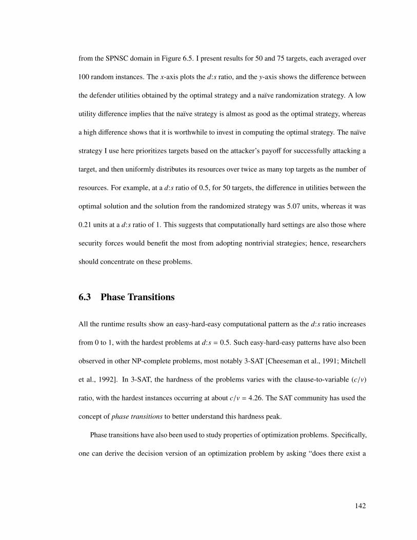
from the SPNSC domain in Figure 6.5. I present results for 50 and 75 targets, each averaged over

100 random instances. The x-axis plots the d:s ratio, and the y-axis shows the difference between

the defender utilities obtained by the optimal strategy and a naıve randomization strategy. A low

utility difference implies that the naıve strategy is almost as good as the optimal strategy, whereas

a high difference shows that it is worthwhile to invest in computing the optimal strategy. The naıve

strategy I use here prioritizes targets based on the attacker’s payoff for successfully attacking a

target, and then uniformly distributes its resources over twice as many top targets as the number of

resources. For example, at a d:s ratio of 0.5, for 50 targets, the difference in utilities between the

optimal solution and the solution from the randomized strategy was 5.07 units, whereas it was

0.21 units at a d:s ratio of 1. This suggests that computationally hard settings are also those where

security forces would benefit the most from adopting nontrivial strategies; hence, researchers

should concentrate on these problems.

6.3 Phase Transitions

All the runtime results show an easy-hard-easy computational pattern as the d:s ratio increases

from 0 to 1, with the hardest problems at d:s = 0.5. Such easy-hard-easy patterns have also been

observed in other NP-complete problems, most notably 3-SAT [Cheeseman et al., 1991; Mitchell

et al., 1992]. In 3-SAT, the hardness of the problems varies with the clause-to-variable (c/v)

ratio, with the hardest instances occurring at about c/v = 4.26. The SAT community has used the

concept of phase transitions to better understand this hardness peak.

Phase transitions have also been used to study properties of optimization problems. Specifically,

one can derive the decision version of an optimization problem by asking “does there exist a

142

0  

1  

2  

3  

4  

5  

6  

7  

0   0.2   0.4   0.6   0.8   1  

U-lity

 

d:s  ra-o  

U-lity  Difference  (50  Targets)  

U-lity  Difference  (75  Targets)  

Figure 6.5: The difference between expected defender utilities from ERASER and a naıve random-ization policy. The vertical line shows d:s = 0.5.

solution with objective function value ≥ k?”, and then looking for a phase transition in the decision

problem. This approach was pioneered by Gent et al. [Gent and Walsh, 1995], who studied the

properties of four different optimization problems including TSP and Boolean circuit synthesis.

They computed the optimal tour length from the TSP optimization problem, and then used this

value as k to define the decision version of the TSP instance. They showed that a phase transition

in the solubility of this problem corresponded to the computationally hardest region. The same

approach was later also used by Gent and Walsh [Gent and Walsh, 1996].

In the context of game theory, phase transitions have been used to analyze the efficiency of

markets in adaptive games [Savit et al., 1999] and the probability of cooperation in evolutionary

game theory [Hauert and Szab, 2005]. To my knowledge, this work is the first that identifies such

structural properties in the context of Stackelberg security games.

143

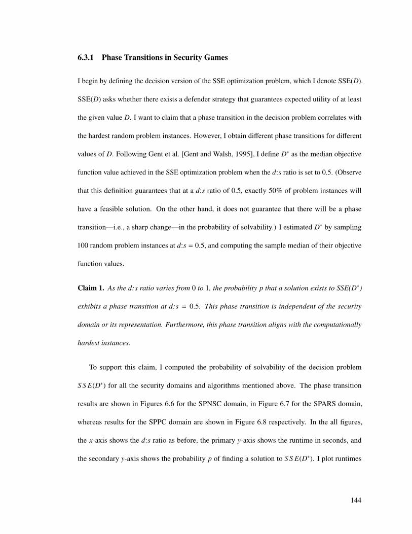
6.3.1 Phase Transitions in Security Games

I begin by defining the decision version of the SSE optimization problem, which I denote SSE(D).

SSE(D) asks whether there exists a defender strategy that guarantees expected utility of at least

the given value D. I want to claim that a phase transition in the decision problem correlates with

the hardest random problem instances. However, I obtain different phase transitions for different

values of D. Following Gent et al. [Gent and Walsh, 1995], I define D∗ as the median objective

function value achieved in the SSE optimization problem when the d:s ratio is set to 0.5. (Observe

that this definition guarantees that at a d:s ratio of 0.5, exactly 50% of problem instances will

have a feasible solution. On the other hand, it does not guarantee that there will be a phase

transition—i.e., a sharp change—in the probability of solvability.) I estimated D∗ by sampling

100 random problem instances at d:s = 0.5, and computing the sample median of their objective

function values.

Claim 1. As the d:s ratio varies from 0 to 1, the probability p that a solution exists to SSE(D∗)

exhibits a phase transition at d:s = 0.5. This phase transition is independent of the security

domain or its representation. Furthermore, this phase transition aligns with the computationally

hardest instances.

To support this claim, I computed the probability of solvability of the decision problem

S S E(D∗) for all the security domains and algorithms mentioned above. The phase transition

results are shown in Figures 6.6 for the SPNSC domain, in Figure 6.7 for the SPARS domain,

whereas results for the SPPC domain are shown in Figure 6.8 respectively. In the all figures,

the x-axis shows the d:s ratio as before, the primary y-axis shows the runtime in seconds, and

the secondary y-axis shows the probability p of finding a solution to S S E(D∗). I plot runtimes

144

0  

0.5  

1  

0.001  

0.01  

0.1  

1  

10  

100  

0   0.2   0.4   0.6   0.8   1  

Prob

ability  p  

Run

7me  (secon

ds)    

d:s  ra7o  

Varia7on  in  Algorithms:    2  Types,  15  Targets  

Mul7ple  LPs   DOBSS   HBGS     Probability  p  

(a)

0  

0.5  

1  

0.001  

0.01  

0.1  

1  

10  

100  

0   0.2   0.4   0.6   0.8   1  

Prob

ability  p  

Run7

me  (secon

ds)    

d:s  ra7o  

DOBSS  Run7me:  2  Types  

10  Targets   15  Targets  

Probability  p  (10  targets)   Probability  p  (15  targets)  

(b)

0  

0.5  

1  

0.01  

0.1  

1  

10  

0   0.2   0.4   0.6   0.8   1  

Prob

ability  p  

Run

7me  (secon

ds)    

d:s  ra7o  

DOBSS  Run7me:  10  Targets  

2  Types   3  Types  

Probability  p  (2  Types)   Probability  p  (3  Types)  

(c)

0  

0.5  

1  

0.001  0.01  0.1  1  10  

100  1000  

0.00   0.20   0.40   0.60   0.80   1.00  

Prob

ability  p  

Run7

me  (secon

ds)    

d:s  ra7o  

Brass:  2  Types  

15  Targets   10  Targets  

Probability  p  (15  Targets)   Probability  p  (10  Targets)  

(d)

0  

0.5  

1  

0  

0.4  

0.8  

1.2  

1.6  

2  

0   0.2   0.4   0.6   0.8   1  

Prob

ability  p  

Run7

me  (secon

ds)  

d:s  ra7o  

Eraser  Run7me:  2  Types  

50  Targets   75  Targets  

Probability  p  (50  targets)   Probabiilty  p  (75  targets)  

(e)

0  

0.5  

1  

0  

0.5  

1  

1.5  

2  

0   0.2   0.4   0.6   0.8   1  

Prob

ability  p  

Run7

me  (secon

ds)  

d:s  ra7o  

Varia7on  in  Solu7on  Mechanism:    2  Types,    50  Targets  

CPLEX:  Primal  Simplex   CPLEX:  Dual  Simplex  CPLEX:  Network  Simplex   CPLEX:  Barrier  GLPK  Simplex   Probability  p  

(f)

Figure 6.6: Average runtime of computing the optimal solution for a SPNSC problem instance.The vertical dotted line shows d:s = 0.5.

using solid lines, as before, and plot p using a dashed line. Figure 6.6(c) presents results for the

DOBSS algorithm for the SPNSC domain for 10 targets and 2 and 3 attacker types. As expected,

the d:s ratio of 0.5 corresponds with p = 0.51 as well as the computationally hardest instances;

more interestingly, I observe that p undergoes a phase transition as the d:s grows. Similarly,

Figure 6.7(b) shows results for the ASPEN algorithm for the SPARS domain with 100 targets, 2

targets per schedule and 400 and 500 schedules, and Figure 6.8(a) shows results for the multiple

145

0  

0.5  

1  

1  

10  

100  

0   0.2   0.4   0.6   0.8   1  

Prob

ability  p  

Run7

me  (secon

ds)  

 

d:s  ra7o  

Aspen  Run7me  100  Targets,  500  Schedules  

|S|  =  4   |S|  =  2  Probabiilty  p  (|S|  =  4)   Probability  p  (|S|  =  2)  

(a)

0  

0.5  

1  

0  

2  

4  

6  

8  

0   0.2   0.4   0.6   0.8   1  

Prob

ability  p  

Run7

me  (secon

ds)  

d:s  ra7o  

Aspen:  100  Targets,    2  Targets  per  schedule  

400  Schedules   500  schedules  

Probability  p  (400  schedules)   Probability  p  (500  schedules)  

(b)

0  

0.5  

1  

0  

2  

4  

6  

8  

0   0.2   0.4   0.6   0.8   1  

Prob

ability  p  

Run7

me    (secon

ds)  

d:s  ra7o  

Aspen:  500  Schedules,    2  Targets  Per  Schedule  

100  Targets   50  Targets  

Probability  p  (100  Targets)   Probability  p  (50  Targets)  

(c)

Figure 6.7: Average runtime of computing the optimal solution for a SPARS game using ASPEN.The vertical dotted line shows d:s = 0.5.

attacker SPPC domain for 1 defender resource. In both cases, I again observe a phase transition in

p. The runtime results of ERASER varying the number of attacker types are shown in Figure 6.9.

The x-axis shows the d:s ratio, whereas the y-axis shows the runtime in seconds.

One might wonder how I can decide that the increase in p is steep enough to be called a phase

transition. I know from both the experimental and theoretical literature on phase transitions in

decision problems that the transition becomes steeper as problem size increases, approaching a

step function in the limit [Kirkpatrick and Selman, 1994; Friedgut, 1998]. This is a property that

I can check for experimentally. I conducted experiments in the SPNSC domain, since it is the

easiest to solve at widely varying problem sizes; the results are shown in Figure 6.10. The x-axis

shows the d:s ratio, and the y-axis shows the probability p of finding a feasible solution to the

decision version of a corresponding SPNSC problem; I plot results for problem instances with 50,

146

0  

0.5  

1  

0.1  

1  

10  

100  

1000  

0.00   0.20   0.40   0.60   0.80   1.00  

Run-me  (seconds)    

d:s  ra-o  

Mul-ple  A<ackers:  1  resource  8  Targets   6  Targets  

Probability  p  (8  targets)   Probability  p  (6  targets)  

(a)

0  

0.5  

1  

1.00  

10.00  

100.00  

1000.00  

0.00   0.20   0.40   0.60   0.80   1.00  

Prob

ability  p  

Run

7me  (secon

ds)  

d:s  ra7o  

Mul7ple  AAackers:  8  Targets  1  Resource   2  Resources  

Probability  p  (1  resource)   Probability  p  (2  resources)  

(b)

0  

0.5  

1  

0.1  

1  

10  

100  

0.00   0.20   0.40   0.60   0.80   1.00  

Prob

ability  p  

Run7

me  (seo

ncds)  

d:s  ra7o  

Bayesian  Single  ACacker:  8  Targets,  1  resource  1  Type   2  Types  

Probability  p  (1  Type)   Probability  p  (2  Types)  

(c)

Figure 6.8: Average runtime for computing the optimal solution for a patrolling domain. Thevertical dotted line shows d:s = 0.5.

0  

0.5  

1  

0  

0.5  

1  

1.5  

2  

2.5  

0   0.2   0.4   0.6   0.8   1  

Run-

me  (secon

ds)  

d:s  ra-o  

Eraser  Run-me:  50  targets  

2  Types   3  Types  

Probability  p  (2  Types)   Probability  p  (3  types)  

Figure 6.9: ERASER results with varying number of attacker types.

100 and 150 targets. I observe the desired result: the phase transition indeed becomes sharper as

the number of targets increases.

147

0  

0.5  

1  

0.3   0.4   0.5   0.6   0.7  

Prob

ability  p  

d:s  ra'o  

50  Targets  

100  Targets  

150  Targets  

Figure 6.10: Probability that the decision problem S S E(D∗) is soluble for SPNSC instances ofthree problem sizes. The phase transition gets sharper as the problem size increases.

148

Chapter 7: Related Work

There exists related work both in game-theoretic as well as non-game theoretic literature studying

the security domain. Much of this work is theoretical analysis of hypothetical scenarios, while my

thesis focuses on algorithms designed for use in real-world security operations. There are three

main areas of related work:

1. The first area is on computation for Stackelberg security games.

2. The second area of related work applies Stackelberg games to other security scenarios.

3. The third area of related work applies other optimization techniques to model the security

domain.

I now explore these three areas in detail.

7.1 Computation in Stackelberg Security Games

The first area of related work is on efficient algorithms for Stackelberg security games, such as

the ones studied in this paper. Game-theoretic models have been applied in a variety of homeland

security settings, such as protecting critical infrastructure [Brown et al., 2006; Pita et al., 2008;

Nie et al., 2007; Kiekintveld et al., 2009] and computer network security [Lye and Wing, 2005;

149

Srivastava et al., 2005], and different algorithms have been developed for such models. The

related work on these game-theoretic approaches for security can be broadly sub-divided into three

categories:

1. Algorithms on computing Stackelberg equilibria,

2. Algorithms to account for human behavior, and

3. Algorithms for computing robust defender strategies.

7.1.1 Efficient computation of Stackelberg equilibria

Within this area of efficient algorithms, the MultipleLPs approach [Conitzer and Sandholm, 2006]

was the first to propose optimal computation of leader strategies in a Stackelberg game. While

this paper did not envision a security scenario, security domains led to a requirement of Bayesian

Stackelberg games. A Bayesian Stackelberg game can be converted to a Stackelberg game by

using the Harsanyi transformation [Harsanyi and Selten, 1972]; however, the size of the Harsanyi

transformed matrix would grow exponentially with the number of attacker types, inhibiting

application for large input problems. The MultipleLPs approach [Conitzer and Sandholm, 2006]

computed optimal defender strategies by operating on the Harsanyi transformed matrix [Harsanyi

and Selten, 1972]; while it did not explicitly represent the Harsanyi transformed matrix in memory,

it required computing solutions to exponentially many linear programs. DOBSS [Paruchuri et al.,

2008b] avoided this Harsanyi transformation, and was the first mixed-integer linear program

proposed for computing optimal defender strategies for the Stackelberg security games. While

DOBSS was much faster that Multiple LPs [Conitzer and Sandholm, 2006], it still requires the

150

input to explicitly represent all the pure strategies of the defender and hence does not scale to

domains with thousands of targets and tens of resources.

Continuing with the first area of related work, Origami is a polynomial time algorithm that

computes optimal defender strategies for a security game when no scheduling constraints are

present (an example of scheduling constraints is the logistical constraints faced by a federal

air marshal). ERASER-C, then, a mixed-integer linear program [Kiekintveld et al., 2009] was

developed for larger and more complex Stackelberg security games. ERASER-C focuses on games

with large numbers of defenders with scheduling constraints, handling the combinatorial explosion

in the defender’s joint schedules. Unfortunately, as the authors note, ERASER-C may fail to

generate a correct solution in cases where arbitrary schedules with more than two flights (e.g.,

multi-city flight tours) are allowed in the input, or when the set of flights cannot be partitioned into

distinct sets for departure and arrival flights. ERASER-C avoids enumerating joint schedules to

gain efficiency, but loses the ability to correctly model arbitrary schedules. Furthermore, ERASER-

C only outputs a coverage vector c, where ct is the probability of the defender protecting target t.

It does not provide the mixed strategy x over joint schedules J of all defender resources, which is

necessary to implement the coverage c in practice. Additionally, no other algorithm has yet been

provided to convert marginals to probabilities over joint schedules, and in Section 3.2, we present

the first efficient algorithm that addresses this challenge for arbitrary scheduling constraints.

The most recent algorithm employing large-scale optimization methods to solve Bayesian

Stackelberg games is HUNTER [Yin and Tambe, 2012]. It employs Benders decomposition [Bert-

simas and Tsitsiklis, 1994] and cut-generation, however, it is not designed to compute optimal

strategy for a defender with scheduling constraints. Double-oracle based approaches that use

both cut and column generation have also been proposed for security games [Halvorson et al.,

151

2009a; Jain et al., 2011b], however, they have only been applied for zero-sum settings. We present

algorithms that are not restricted to the strict zero-sum requirement of the previous algorithms,

but instead operate on Stackelberg security games [Kiekintveld et al., 2009]. In a security game,

protecting a target is always beneficial for the defender and worse for the attacker, however, the

payoffs need not be zero-sum.

In contrast, Aspen employs the technique of branch-and-price [Barnhart et al., 1994] and

computes solutions for a Stackelberg security game with arbitrary scheduling constraints. Addi-

tionally, hierarchical decomposition methods like the one employed by Hbsa have also not seen

much application towards obtaining optimal solutions in Bayesian Stackelberg games, although

similar techniques have been proposed to obtain approximate Nash equilibrium for symmetric

games [Wellman et al., 2005].

Game theory has also been applied to a wide range of problems where one player — the evader

— tries to minimize the probability of detection by and/or encounter with the other player — the

patroller; the patroller wants to thwart the evader’s plans by detecting and/or capturing him. The

formalization of this problem led to a family of games, often called pursuit-evasion games [Adler

et al., 2002]. As there are many potential applications of this general idea, more specialized game

types have been introduced, e.g., hider-seeker games [Flood, 1972; Halvorson et al., 2009b] and

infiltration games [Alpern, 1992] with mobile patrollers and mobile evaders; search games [Gal,

1980] with mobile patrollers and immobile evaders; and ambush games [Ruckle et al., 1976] with

the mobility capabilities reversed. In the game model proposed in this paper, the evader is mobile

whereas the patroller is not, just like in ambush games. However, in contrast with ambush games,

we consider targets (termed destinations in ambush games) of varying importance.

152

The network security game model described in this thesis is most similar to that of interdiction

games [Washburn and Wood, 1995], where the evading player — the attacker — moves on an

arbitrary graph from one of the origins to one of the destinations (aka. targets); and the interdicting

player — the defender — inspects one or more edges in the graph in order to detect the attacker

and prevent him from reaching the target. As opposed to interdiction games, we do not consider

the detection probability on edges, but we allow different values to be assigned to the targets,

which is crucial for real-world applications.

Recent work has also considered scheduling multiple-defender resources using cooperative

game-theory, as in path disruption games [Bachrach and Porat, 2010], where the attacker tries

to reach a single known target. In contrast with the static asset protection problem [Dickerson

et al., 2010a], we attribute different importance to individual targets and unlike its dynamic

variant [Dickerson et al., 2010a], we consider only static target positions. Recent work in security

games and robotic patrolling [Basilico et al., 2009; Jain et al., 2010b] has focused on concrete

applications. However, they have not considered the scale-up for both defender and attacker

strategies. For example, in ASPEN, the attacker’s pure strategy space is polynomially large, since

the attacker is not following any path and just chooses exactly one target to attack. Our game model

was introduced by Tsai et al. [Tsai et al., 2010]; however, their approximate solution technique

can be suboptimal. We discuss the shortcomings of their approach in Section 4.1, and provide an

optimal solution algorithm for the general case.

Finally, algorithms that model security domains using Stackelberg games have seen many

real-world deployments. ARMOR [Pita et al., 2008; Jain et al., 2010c] is a software assistant

deployed at the Los Angeles International Airport since August 2007 that casts the scheduling

problem of vehicular checkpoints and canine patrols as a Stackelberg game and uses the DOBSS

153

algorithm to compute these schedules. Similarly, the IRIS [Jain et al., 2010c] scheduling system,

in use by the United States Federal Air Marshal Service since October 2009, generates schedules

over international flights for the air marshals using the Aspen algorithm presented in this thesis.

Similarly, GUARDS [Pita et al., 2011b] is also a game-theoretic scheduling system in use by

the United States Transport Security Administration to randomize behind-the-scenes activities

conducted by the security agency. In the same way, PROTECT [An et al., 2011], another software

scheduling system based on Stackelberg games, has been in use by the Boston Coast Guard since

April 2011 to generate patrol routes for the boats and other resources available to the Boston

Coast Guard. Finally, TRUSTS [Yin et al., 2012c] is another software scheduling system based on

Stackelberg games that has been in use by the Los Angeles Sheriff’s Department since May 2012

to generate strategies for the officers to inspect passengers towards reducing crime and suppressing

fare evasion on the Los Angeles metro transit system.

7.1.2 Stackelberg equilibria modeling humans

The second category of related work that applies game-theory to security domains computes

defender strategies when faced against human adversaries. This work takes into account the

biases and bounded rationality of a human opponent. Cobra is one such algorithm that considers

anchoring-bias of humans [Pita et al., 2009], as well as attacker indifference between pure strategies

that are at most ε away from the optimal. Alternate solution techniques grounded in psychological

concepts like Quantal Response Equilibrium (QRE) have also been proposed [Yang et al., 2011].

The focus of these algorithms has been to develop algorithms that perform well against humans;

indeed they have been evaluated against human subjects. My research is complimentary to this

154

work; and my techniques of column generation are now being combined with Quantal response

and other models of human-decision making.

7.1.3 Computation of robust solutions

The third category of related work aims at computing robust solutions. Kiekintveld et. al [Kiek-

intveld et al., 2011] model distributions over preferences of an attacker using infinite Bayesian

games, and propose an algorithm to generate approximate solutions for such games. Yin et. al [Yin

et al., 2012a] also provide robust solutions in the presence of execution and observation errors.

The Cobra algorithm [Pita et al., 2009] mentioned before focuses on ε-rationality of the attacker,

specifically for human subjects. In contrast, Yin et. al [Yin et al., 2010a] consider the limiting

case where an attacker has no observations and thus investigate the equivalence of Stackelberg vs

Nash equilibria. Even earlier investigations have emphasized the value of commitment to mixed

strategies in Stackelberg games in the presence of noise [van Damme and Hurkens, 1997]. Secrecy

and deception have also been modeled for Stackelberg games [Zhuang and Bier, 2011]. Outside

of Stackelberg games, models for execution uncertainty in game-theory have been separately

developed [Archibald and Shoham, 2009]. Robust solution methods for simultaneous move games

have also been studied [Aghassi and Bertsimas, 2006; Porter et al., 2002].

7.2 Stackelberg games in other security scenarios

The second area of related work applies Stackelberg games to other security scenarios. Lawrence

et al [Wein, 2008] apply Stackelberg games in the context of screening visitors entering the US. In

their work, they model the U.S. Government as the leader who specifies the biometric identification

155

strategy to maximize the detection probability using finger print matches, and the follower is

the terrorist who can manipulate the image quality of the finger print. Stackelberg games have

also been used for studying missile defense systems [Brown et al., 2005a] and for studying the

development of an adversary’s weapon systems [Brown et al., 2005b]. A family of Stackelberg

games known as inspection games is closely related to the security games we are interested in

and includes models of arms inspections and border patrols [Avenhaus et al., 2002]. Another

line of recent work is on randomized security and robotic patrolling using Stackelberg games for

generic “police and robbers” scenario [Gatti, 2008; Amigoni et al., 2008; Basilico et al., 2009].

These models use extensive form games to model the domain and present alternative algorithms to

patrolling domains.

7.3 Other optimization techniques for security domains

The third area of related work applies other optimization techniques to model the security domain,

but does not address the strategic aspects of the problem. These methods provide a randomization

strategy for the defender, but they do not take into account the fact that the adversaries can observe

the defender’s actions and then adjust their behavior. Examples of such approaches include [Ruan

et al., 2005; Paruchuri et al., 2006] which are based on learning, Markov Decision Processes

(MDPs) and Partially Observable Markov Decision Processes (POMDPs). As part of this work,

the authors model the patrolling problem with locations and varying incident rates in each of

the locations and solve for optimal routes using a MDP framework. Another example is the

“Hypercube Queueing Model” [Larson, 1974] which is based on queueing theory and depicts the

detailed spatial operation of urban police departments and emergency medical services. It has

156

found application in police beat design, in allocation of patrolling time, etc. Babu et al [Babu

et al., 2006] have worked on modeling passenger security system at US airports using linear

programming approaches, however, their objective is to classify the passengers in various groups

and then screen them based on the group they belong to. Similarly, Agmon et. al [Agmon et al.,

2008] analyze the performance of an attacker with zero-knowledge, and an attacker with partial

knowledge in a perimeter patrolling domain. Such frameworks can address many of the problems

we raise, including different target values and increasing uncertainty by using many possible patrol

routes. However, they fail to account for the possibility that an intelligent attacker will observe and

exploit patterns in the security policy. If a policy is based on the historical frequency of attacks, it

is essentially a reactive policy and an intelligent attacker will always be one step ahead.

157

Chapter 8: Conclusions

Game-theoretic approaches have shown their usefulness in deployed security applications such

as ARMOR for the Los Angeles International Airport Pita et al. [2008], IRIS for the Federal Air

Marshal Service Jain et al. [2010a], Guards for the Transportation Security Administration Pita

et al. [2011a], PROTECT for the Boston Coast Guard Shieh et al. [2012], and TRUSTS for the

Los Angeles Metro Rail System Yin et al. [2012b]. At the core of the these applications is the

Stackelberg game model. A solution to these Stackelberg games yields the optimal mixed strategy,

or the optimal allocation of the defender’s resources.

However, game theoretic models for real-world problems can have trillions of pure strategies

for both players. Thus, scalable algorithms to solve these game-theoretic models are thus required

to obtain solutions for real-world domains: e.g., scheduling 10 air marshals to protect 100 flights

yields(10010

)≈ 1.7 × 1013 unique assignments (or pure strategies) for the defender. Such large

models cannot even be stored in the memory of computers today, let alone be solved by existing

algorithms. I have provided algorithms especially designed to scale-up to exponentially many pure

strategies for both players, as required to compute solutions for large real-world domains. My

research on computational game theory provides algorithms that have enabled optimal solutions to

158

be computed for domains with: (i) trillions of strategies for the defender, (ii) trillions of strategies

for the attacker, and (iii) Bayesian Stackelberg games with many adversary types.

These algorithms avoid representing the entire game in memory, while computing solutions

for the entire large problem. These algorithms are built on the following insights: (i) Real-

world domains have exponentially many pure strategies for the defender (e.g. a combination of

checkpoints), and so, an incremental approach of generating pure strategies of the defender is

required. This will avoid enumerating all the pure strategies, and will only add a pure strategy if

the pure strategy would help increase defender payoff. (ii) In domains with exponentially many

attacker pure strategies, an incremental approach to generate pure strategies for the attacker (e.g.

attack paths) should be used to avoid enumeration of the pure strategy set of the attacker. (iii) A

Bayesian Stackelberg game can be decomposed into hierarchically-organized smaller games, each

with smaller number of attacker types, providing heuristics which can be used to eliminate the

never-best-response (that is, dominated) pure strategies of the attacker. I also provide mathematical

guarantees for the obtained solutions: the algorithms can compute the globally optimal solution

and can also be tuned to return an approximate solution with quality guarantees.

These insights provide speed-ups by reducing the size of the game: while insights on strategy

generation restrict the game size by efficiently generating sub-games that include a pure strategy

only if it improves the player’s payoff, the hierarchical approach pre-processes the input Bayesian

Stackelberg game instance and removes the attacker pure strategies that cannot be part of the

optimal solution. Furthermore, I have investigated what properties of Stackelberg security game

instances make them hard to solve in practice, across different input sizes and different security

domains. The algorithms developed in my thesis have also been deployed in the real-world.

159

8.1 Contributions

While previous algorithms could not scale to domains with more than 1000 pure strategies

in Stackelberg games, my thesis provides novel algorithms built on large-scale optimization

techniques that scale to billions of pure strategies for both players. My thesis made the following

contributions:

• Aspen: I designed Aspen [Jain et al., 2010b] for large security problems with arbitrary

scheduling constraints, e.g., the problem of scheduling air marshals on board flights. Aspen

builds on the large-scale optimization approach of branch-and-price, which uses a combina-

tion of branch-and-bound, linear programming and network flows to efficiently compute the

solution. In fact, Aspen is the algorithm that powers the IRIS system.

• Rugged and Snares: I designed Rugged for domains where both the defender and the

attacker have billions of pure strategies and they operate on a network [Jain et al., 2011b],

e.g., when considering cyber-security or protection of an urban road network. The Rugged

algorithm uses a double-oracle methodology, which is similar to column/cut generation

approaches proposed in operations research. The Rugged algorithm laid the foundation for

Snares, which exploiting sub-modularity properties in the problem, built on Rugged, and

provided orders of magnitude speed-ups [Jain et al., 2013]. We are, in fact, in discussions

with the police force of Mumbai, India to see how Snares may be made available to them

for deploying checkpoints on the roads of Mumbai.

• Hbgs and Hbsa: Furthermore, modeling uncertainty is an important challenge when fo-

cusing on real-world domains. Uncertainty is modeled through the Bayesian extension of

Stackelberg games. I thus developed an efficient computational approach for solving large

160

Bayesian Stackelberg games, or Stackelberg games with many attacker types. I proposed

a hierarchical methodology of decomposing large Bayesian Stackelberg games into many

smaller Bayesian Stackelberg games, and provided a framework to use the solutions to

these smaller games to efficiently apply branch-and-bound on the original large Bayesian

Stackelberg game. Using this hierarchical methodology, I have provided two algorithms:

Hbgs and Hbsa tailored to compute efficient solutions with and without arbitrary scheduling

constraints respectively [Jain et al., 2011a].

• Deployment-to-Saturation ratio: I have studied problem instances for Stackelberg games

broadly to identify the properties that make a problem instance computationally challenging.

I formalized the concept of the deployment-to-saturation (d:s) ratio in Stackelberg security

games, and showed that problem instances for which d:s = 0.5 are computationally harder

than instances with other d:s ratios for a wide range of different domains, algorithms, solvers

or equilibrium computation methods [Jain et al., 2012]. This work also provides evidence

that the computationally hard region is also one where optimization is most beneficial to the

real-world security agencies, corroborating the need for algorithmic advances. Furthermore,

I use the concept of phase transitions to better understand this computationally hard region.

• Deployments – ARMOR and IRIS: My work has also been deployed in the real-world: I

have developed algorithms for and subsequently led the building of the IRIS system that

is used by the Federal Air Marshals Service (FAMS) to schedule air marshals on board

international commercial flights since October 2009 [Jain et al., 2010c]. I also worked on

the ARMOR system, which is in use by the Los Angeles airport police [Pita et al., 2008].

Furthermore, the success of IRIS and ARMOR systems has led to newer deployments

161

of such algorithms in other real-world security domains, like the PROTECT system for

the U.S. Coast Guard [Shieh et al., 2012], and the TRUSTS system for the LA Sheriff

Department [Yin et al., 2012b].

8.2 Future Plans

The research described in this thesis is driven by the vision of a world where agent technologies

are widespread, and working to assist decision makers in critical domains, with emphasis on (i)

security, e.g., protecting cyber-networks and transportation systems, (ii) sustainability, e.g., forest

and wildlife conservation, and (iii) safety, e.g., health care and disaster response.

The mathematical framework of game theory is appropriate for analyzing decision making for

all these domains. However, there are three significant research areas that need to be developed

towards my vision: (i) Scalable behavioral game theory: computing solutions for large real-

world domains in the presence of humans, who may be boundedly rational or have limited

computationally capability; (ii) Stochastic coalitional game theory: analyzing decision making for

a team of agents in an uncertain environment; and (iii) Spatiotemporal game theory: performing

computations over continuous space and time. My current research has focused on addressing

these challenges, with the focus of my Ph.D. thesis being scalable game theoretic algorithms. I

briefly describe these pillars of game theory below.

8.2.1 Scalable behavioral game theory

Scalable algorithms that incorporate human decision making are required to obtain game-theoretic

solutions for real-world domains. This is required since real human adversaries do not necessarily

162

act according to abstract models of rationality, since they may have cognitive biases, limited

computational ability and uncertain or incomplete information. Instead, humans may rely on

heuristics and simplified abstractions for their decision making, which is not captured in traditional

game-theoretic models. The insights proposed in my thesis have led to algorithms that can scale to

real-world sizes; now these algorithms are being extended with models of human decision making.

I have earlier co-developed game-theoretic algorithms that exploit insights from behavioral models

like anchoring bias [Pita et al., 2009], and algorithms using strategy generation for achieving

scalability and using quantal response for human decision making are forthcoming. However,

much more remains to be done in developing scalable algorithms that perform better against

humans individually or in groups.

8.2.2 Stochastic coalitional game theory

Many real-world domains have multiple teams of agents, where agents in one team cooperate and

coordinate to jointly achieve a common goal. This coordination between agents leads to coalition

structures; however, in real-world domains, such coalitions may face uncertainty and adversaries.

Payoffs to the team depend on the combination of actions taken by the individual team members,

and these payoffs may also vary over time.

Distributed Constraint Optimization Problems (DCOPs) framework is proposed in literature

for coordinating between multiple agents, and provides a basis for coalition games. However,

DCOPs are limited since they do not handle stochasticity. Thus, I have defined a new class of

Distributed Coordination of Exploration and Exploitation (DCEE) [Jain et al., 2009; Taylor et al.,

2010] problems, that balance the exploration and exploitation of multiple mobile agents (e.g.,

163

for robot navigation in buildings for post disaster recovery); I developed novel algorithms and

implemented them on actual iRobot Creates.

Coalition formation among agents is a key aspect of real-world decision making, in both

non-adversarial as well as adversarial domains. A coalition of adversaries who may not have

perfectly-aligned goals must negotiate with each other on who pays which cost or who receives

what benefits. Similarly, a coalition of defenders may have teams with different skill sets and

goals. It is also critical to understand the dynamic nature of how these relationships form and

change. I plan to use DCEE for analyzing defender coalitions in adversarial settings by researching

equilibrium analysis of such games, as well as investigate strategic adaptation over time, based on

both sound mathematical principles and human behavioral models.

8.2.3 Spatiotemporal game theory

Adversarial domains in the real world require both the defenders and the attackers to act in a

geographical space, and in continuous time. Incorporating spatiotemporal modeling in game theory

requires novel research — current work often does not model continuous spaces and continuous

time. Incorporating spatiotemporal reasoning will improve our ability to address domains such

as protection of large forest areas or fisheries of the world or protecting endangered species, and

help us generate more effective strategies for the defender. This field has not seen much focus; a

situation that I would like to redress.

In summary, for my future work, inspired by real-world challenges of security, sustainability

and safety, my vision is to take on fundamental challenges that arise in taking computational game

theory into the real world: in problem domains that range from physical security to cybersecurity

to forest protection to conservation of wildlife to disaster rescue and management. To address

164

these fundamental challenges, I would like to conduct basic research built on foundations of

interdisciplinary connections to economics, operations research, psychology, health, and law

among other disciplines.

165

Bibliography

Air Traffic Control: By the Numbers. http://www.natca.org/mediacenter/bythenumbers.msp,2011.

Micah Adler, Harald Racke, Naveen Sivadasan, Christian Sohler, and Berthold Vocking. Random-ized pursuit-evasion in graphs. In ICALP, pages 901–912, 2002.

Michele Aghassi and Dimitris Bertsimas. Robust Game Theory. Math. Program., 107:231–273,June 2006.

Noa Agmon, Vladimir Sadov, Gal A. Kaminka, and Sarit Kraus. The Impact of AdversarialKnowledge on Adversarial Planning in Perimeter Patrol. In Proceedings of the InternationalConference on Autonomous Agents and Multiagent Systems (AAMAS), volume 1, pages 55–62,2008.

S. Alpern. Infiltration Games on Arbitrary Graphs. Journal of Mathematical Analysis andApplications, 163:286–288, 1992.

Francesco Amigoni, Nicola Gatti, and Antonio Ippedico. A game-theoretic approach to de-termining efficient patrolling strategies for mobile robots. In Proceedings of the 2008IEEE/WIC/ACM International Conference on Web Intelligence and Intelligent Agent Tech-nology - Volume 02, WI-IAT ’08, pages 500–503, Washington, DC, USA, 2008. IEEEComputer Society. ISBN 978-0-7695-3496-1. doi: 10.1109/WIIAT.2008.324. URLhttp://dx.doi.org/10.1109/WIIAT.2008.324.

Bo An, James Pita, Eric Shieh, Milind Tambe, Chris Kiekintveld, and Janusz Marecki.Guards and protect: next generation applications of security games. SIGecom Exch.,10(1):31–34, March 2011. ISSN 1551-9031. doi: 10.1145/1978721.1978729. URLhttp://doi.acm.org/10.1145/1978721.1978729.

Christopher Archibald and Yoav Shoham. Modeling Billiards Games. In Proceedings of theInternational Conference on Autonomous Agents and Multiagent Systems (AAMAS), 2009.

Rudolf Avenhaus, Bernhard von Stengel, and Shmuel Zamir. Inspection Games. In Robert J.Aumann and Sergui Hart, editors, Handbook of Game Theory, volume 3, chapter 51, pages1947–1987. North-Holland, Amsterdam, 2002.

L. Babu, L. Lin, and R. Batta. Passenger Grouping Under Constant Threat Probability in anAirport Security System. In European Journal of Operational Research, volume 168, pages 633– 644, 2006.

166

Yoram Bachrach and Ely Porat. Path Disruption Games. In AAMAS, pages 1123–1130, 2010.

C. Barnhart, E.L. Johnson, G.L. Nemhauser, M.W.P. Savelsbergh, and P.H. Vance. Branchand Price: Column Generation for Solving Huge Integer Programs. In Operations Research,volume 46, pages 316–329, 1994.

Tamer Basar and Geert Jan Olsder. Dynamic Noncooperative Game Theory. Academic Press, SanDiego, CA, 2nd edition, 1995.

N. Basilico, N. Gatti, and F. Amigoni. Leader-Follower Strategies for Robotic Patrolling inEnvironments with Arbitrary Topologies. In Proceedings of the International Conference onAutonomous Agents and Multiagent Systems (AAMAS), pages 500–503, 2009.

Dimitris Bertsimas and John N. Tsitsiklis. Introduction to Linear Optimization. Athena Scientific,1994.

Mikel Blanco, Aurelia Valino, Joost Heijs, Thomas Baumert, and Javier Gonzalez Gomez. TheEconomic Cost of March 11: Measuring the direct economic cost of the terrorist attack onMarch 11, 2004 in Madrid. Terrorism and Political Violence, 19(4):489–509, 2007.

Branislav Bosansky, Viliam Lisy, Michal Jakob, and Michal Pechoucek. Computing Time-Dependent Policies for Patrolling Games with Mobile Targets. In Tenth International Conferenceon Autonomous Agents and Multiagent Systems, pages 989–996, 2011.

Michele Breton, A. Alg, and Alain Haurie. Sequential Stackelberg Equilibria in Two-PersonGames. Optimization Theory and Applications, 59(1):71–97, 1988.

G. Brown, M. Carlyle, J. Kline, and K. Wood. A Two-Sided Optimization for Theater BallisticMissile Defense. In Operations Research, volume 53, pages 263–275, 2005a.

G. Brown, M. Carlyle, J. Royset, and K. Wood. On The Complexity of Delaying an Adversary’sProject. In B. Golden, S. Raghavan, and E. Wasil, editors, The Next Wave in Computing,Optimization and Decision Technologies, pages 3–17. Springer, 2005b.

Gerald Brown, Matthew Carlyle, Javier Salmeron, and Kevin Wood. Defending Critical Infrastruc-ture. In Interfaces, volume 36, pages 530 – 544, 2006.

Rina Chandran and Greg Beitchman. Battle for Mumbai Ends, Death Toll Rises to 195. Times ofIndia, 29 November 2008.

Peter Cheeseman, Bob Kanefsky, and William M. Taylor. Where the Really Hard Problems are. InProceedings of the International Joint Conference on Artificial Intelligence, pages 331–337,1991.

CNN. Sources: Air Marshals missing from almost all flights. 2008.http://articles.cnn.com/2008-03-25/travel/siu.air.marshals 1 air-marshals-federal-air-flights? s=PM:TRAVEL/.

Vincent Conitzer and Tuomas Sandholm. Computing the Optimal Strategy to Commit to. InProceedings of the ACM Conference on Electronic Commerce (ACM-EC), pages 82–90, 2006.

167

John Dickerson, Gerardo Simari, V.S. Subrahmanian, and Sarit Kraus. A Graph-TheoreticApproach to Protect Static and Moving Targets from Adversaries. In AAMAS, pages 299–306,2010a.

J.P. Dickerson, G.I. Simari, V.S. Subrahmanian, and Sarit Kraus. A Graph-Theoretic Approach toProtect Static and Moving Targets from Adversaries. In Proceedings of the Ninth InternationalConference on Autonomous Agents and Multiagent Systems (AAMAS-2010), pages 299–306,2010b.

David Eppstein and Michael T. Goodrich. Studying (Non-Planar) Road Networks Through anAlgorithmic Lens. CoRR, abs/0808.3694, 2008.

Merrill M. Flood. The Hide and Seek Game of Von Neumann. MANAGEMENT SCIENCE, 18(5-Part-2):107–109, 1972.

Jeremy Frank, Ian P. Gent, and Toby Walsh. Asymptotic and Finite Size Parameters forPhase Transitions: Hamiltonian Circuit as a Case Study. Inf. Process. Lett., 65:241–245,March 1998. ISSN 0020-0190. doi: http://dx.doi.org/10.1016/S0020-0190(97)00222-6. URLhttp://dx.doi.org/10.1016/S0020-0190(97)00222-6.

Ehud Friedgut. Sharp thresholds of graph properties, and the k-sat problem. J. Amer. Math. Soc,12:1017–1054, 1998.

Shmuel Gal. Search Games. Academic Press, New York, 1980.

Nicola Gatti. Game Theoretical Insights in Strategic Patrolling: Model and Algorithm in Normal-Form. In Proceedings of the European Conference on Artificial Intelligence (ECAI), pages403–407, 2008.

Ian P. Gent and Toby Walsh. Phase transitions from real computational problems. In Proceedingsof the 8th International Symposium on Artificial Intelligence, pages 356–364, 1995.

Ian P. Gent and Toby Walsh. The TSP Phase Transition. Artificial Intelligence, 88(12):349 – 358,1996.

M. Haklay and P. Weber. Openstreetmap:user-generated street maps. Pervasive Computing, IEEE,7(4):12–18, 2008.

E. Halvorson, V. Conitzer, and R. Parr. Multi-step multi-sensor hider-seeker games. In IJCAI,pages 336–341, 2009a.

Erik Halvorson, Vincent Conitzer, and Ronald Parr. Multi-step Multi-sensor Hider-Seeker Games.In Proceedings of the International Joint Conference on Artificial Intelligence (IJCAI), pages159–166, 2009b.

J.C. Harsanyi and R. Selten. A Generalized Nash Solution for Two-person Bargaining Games withIncomplete Information. In Management Science, volume 18, pages 80–106, 1972.

Christoph Hauert and Gyrgi Szab. Game theory and Physics. Am. J. Phys., 73(5):405–414, 2005.doi: 10.1119/1.1848514.

168

M. Jain, J. Tsai, J. Pita, C. Kiekintveld, S. Rathi, M. Tambe, and F. Ordonez. Software assistantsfor randomized patrol planning for the LAX Airport Police and the Federal Air Marshals Service.Interfaces, 40:267–290, 2010a.

Manish Jain, Matthew E. Taylor, Milind Tambe, and Makoto Yokoo. Dcop meets the real world:Exploring unknown reward matrices with applications to mobile sensor nets. In IJCAI, 2009.

Manish Jain, Erim Kardes, Christopher Kiekintveld, Fernando Ordonez, and Milind Tambe.Security Games with Arbitrary Schedules: A Branch and Price Approach. In Proceedings of theAAAI Conference on Artificial Intelligence (AAAI), 2010b.

Manish Jain, Jason Tsai, James Pita, Christopher Kiekintveld, Shyamsunder Rathi, Milind Tambe,and Fernando Ordonez. Software Assistants for Randomized Patrol Planning for the LAXAirport Police and the Federal Air Marshals Service. Interfaces, 40:267–290, 2010c.

Manish Jain, Christopher Kiekintveld, and Milind Tambe. Quality-bounded Solutions for FiniteBayesian Stackelberg Games: Scaling up. In Proceedings of the International Conference onAutonomous Agents and Multiagent Systems (AAMAS), 2011a.

Manish Jain, Dmytro Korzhyk, Ondrej Vanek, Vincent Conitzer, Michal Pechoucek, and MilindTambe. A Double Oracle Algorithm for Zero-Sum Security Games on Graphs. In Proceedingsof the International Conference on Autonomous Agents and Multiagent Systems (AAMAS),2011b.

Manish Jain, Kevin Leyton-Brown, and Milind Tambe. The deployment-to-saturation ratio insecurity games. In AAAI, 2012.

Manish Jain, Vincent Conitzer, Michal Pechoucek, and Milind Tambe. Security scheduling forreal-world networks. In AAMAS, 2013.

Albert Jiang and Kevin Leyton-Brown. A polynomial-time algorithm for action-graph games. InArtificial Intelligence, pages 679–684, 2006.

Armen Keteyian. TSA: Federal Air Marshals. 2010.http://www.cbsnews.com/stories/2010/02/01/earlyshow/main6162291.shtml,retrieved Feb 1, 2011.

Christopher Kiekintveld, Manish Jain, Jason Tsai, James Pita, Milind Tambe, and FernandoOrdonez. Computing Optimal Randomized Resource Allocations for Massive Security Games.In Proceedings of the International Conference on Autonomous Agents and Multiagent Systems(AAMAS), pages 689–696, 2009.

Christopher Kiekintveld, Janusz Marecki, and Milind Tambe. Approximation Methods for InfiniteBayesian Stackelberg Games: Modeling Distributional Payoff Uncertainty. In Proceedings ofthe International Conference on Autonomous Agents and Multiagent Systems (AAMAS), 2011.

Scott Kirkpatrick and Bart Selman. Critical behavior in the satisfiability of random booleanformulae. Science, 264:1297–1301, 1994.

169

Daphne Koller and Brian Milch. Multi-agent influence diagrams for representing and solvinggames. Games and Economic Behavior, 45(1):181–221, 2003.

D. Korzhyk, V. Conitzer, and R. Parr. Complexity of Computing Optimal Stackelberg Strategiesin Security Resource Allocation Games. In Proceedings of the AAAI Conference on ArtificialIntelligence (AAAI), pages 805–810, 2010.

Solomon Kullback and Richard A. Leibler. On Information and Sufficiency. The Annals ofMathematical Statistics, 22(1):79–86, 1951.

R.C. Larson. A Hypercube Queueing Modeling for Facility Location and Redistricting in UrbanEmergency Services. In Journal of Computers and Operations Research, volume 1, pages67–95, 1974.

George Leitmann. On Generalized Stackelberg Strategies. Optimization Theory and Applications,26(4):637–643, 1978.

Joshua Letchford and Yevgeniy Vorobeychik. Computing Randomized Security Strategies inNetworked Domains. In Proceedings of the Workshop on Applied Adversarial Reasoning andRisk Modeling (AARM) at AAAI, 2011.

Joshua Letchford, Vincent Conitzer, and Kamesh Munagala. Learning and Approximating theOptimal Strategy to Commit To. In Proceedings of the International Symposium on AlgorithmicGame Theory (SAGT), pages 250–262, 2009.

Robert Looney. Economic Costs to the United States Stemming From the 9/11 Attacks. StrategicInsights, 1(6), August ”2002”.

Kong-wei Lye and Jeannette M. Wing. Game strategies in network security. International Journalof Information Security, 4(1–2):71–86, 2005.

H. Brendan McMahan, Geoffrey J. Gordon, and Avrim Blum. Planning in the Presence of CostFunctions Controlled by an Adversary. In Proceedings of the International Conference onMachine Learning (ICML), pages 536–543, 2003.

D. Mitchell, B. Selman, and H. Levesque. Hard and Easy Distributions of SAT Problems. InProceedings of the American Association for Artificial Intelligence, pages 459–465, 1992.

G. L. Nemhauser, L. A. Wolsey, and M. L. Fisher. An Analysis of Approximations for MaximizingSubmodular Set Functions–I. Mathematical Programming, 14(1):265–294, Dec 1978.

Nie, R. Batta, Drury, and Lin. Optimal Placement of Suicide Bomber Detectors. In MilitaryOperations Research, volume 12, pages 65–78, 2007.

Martin J. Osbourne and Ariel Rubinstein. A Course in Game Theory. MIT Press, 1994.

Praveen Paruchuri, Milind Tambe, Fernando Ordonez, and Sarit Kraus. Security in Multiagent Sys-tems by Policy Randomization. In Proceedings of the International Conference on AutonomousAgents and Multiagent Systems (AAMAS), 2006.

170

Praveen Paruchuri, Jonathan P. Pearce, Janusz Marecki, Milind Tambe, Fernando Ordonez, andSarit Kraus. Playing games with security: An efficient exact algorithm for Bayesian Stackelberggames. In AAMAS-08, pages 895–902, 2008a.

Praveen Paruchuri, Jonathan P. Pearce, Janusz Marecki, Milind Tambe, Fernando Ordonez, andSarit Kraus. Playing Games with Security: An Efficient Exact Algorithm for Bayesian Stack-elberg games. In Proceedings of the International Conference on Autonomous Agents andMultiagent Systems (AAMAS), pages 895–902, 2008b.

J. Pita, C. Kiekintveld, M. Tambe, E. Steigerwald, and S. Cullen. GUARDS - game theoreticsecurity allocation on a national scale. In AAMAS, pages 37–44, 2011a.

James Pita, Manish Jain, Craig Western, Christopher Portway, Milind Tambe, Fernando Ordonez,Sarit Kraus, and Praveen Paruchuri. Deployed ARMOR Protection: The Application of aGame-theoretic Model for Security at the Los Angeles International Airport. In Proceedings ofthe International Conference on Autonomous Agents and Multiagent Systems (AAMAS), IndustryTrack, pages 125–132, 2008.

James Pita, Manish Jain, Fernando Ordonez, Milind Tambe, Sarit Kraus, and Reuma Magori-cohen. Effective solutions for real-world Stackelberg games: When agents must deal withhuman uncertainties. In Proceedings of the International Conference on Autonomous Agentsand Multiagent Systems (AAMAS), 2009.

James Pita, Manish Jain, Fernando Ordonez, Milind Tambe, and Sarit Kraus. Robust Solutionsto Stackelberg Games: Addressing Bounded Rationality and Limited Observations in HumanCognition. Artificial Intelligence Journal, 174(15):1142-1171, 2010, 2010.

James Pita, Christopher Kiekintveld, Milind Tambe, Erin Steigerwald, and Shane Cullen.GUARDS - Game Theoretic Security Allocation on a National Scale. In Proceedings ofthe International Conference on Autonomous Agents and Multiagent Systems (AAMAS), 2011b.

R. Porter, A. Ronen, Y. Shoham, and M. Tennenholtz. Mechanism Design with ExecutionUncertainty. In Proceedings of the Conference on Uncertainty in Artificial Intelligence (UAI),2002.

S. Ruan, C. Meirina, F. Yu, K. R. Pattipati, and R. L. Popp. Patrolling in a Stochastic Environment.In 10th Intl. Command and Control Research and Tech. Symp., 2005.

William Ruckle, Robert Fennell, Paul T. Holmes, and Charles Fennemore. Ambushing RandomWalks I: Finite Models. Operations Research, 24:314–324, 1976.

Todd Sandler and Daniel G. Arce M. Terrorism and Game Theory. Simulation and Gaming, 34(3):319–337, 2003.

Robert Savit, Radu Manuca, and Rick Riolo. Adaptive Competition, Market Efficiency, PhaseTransitions and Spin-Glasses. University of Michigan, 82:2203–2206, 1999.

E. Shieh, B. An, R. Yang, M. Tambe, C. Baldwin, J. DiRenzo, B. Maule, and G. Meyer. PROTECT:An application of computational game theory for the security of the ports of the United States.In AAAI, pages 2173–2179, 2012.

171

John Slaney and Toby Walsh. Phase Transition Behavior: from Decision to Optimization. InProceedings of the 5th International Symposium on the Theory and Applications of SatisfiabilityTesting, SAT, 2002.

Vivek Srivastava, James Neel, Allen B. MacKenzie, Rekha Menon, Luiz A. Dasilva, James E.Hicks, Jeffrey H. Reed, and Robert P. Gilles. Using Game Theory to Analyze Wireless Ad HocNetworks. IEEE Communications Surveys and Tutuorials, 7(4), 2005.

D. Stevens and et. al. Implementing Security Improve-ment Options at Los Angeles International Airport. 2006.http://www.rand.org/pubs/documented briefings/2006/RAND DB499-1.pdf.

Milind Tambe. Security and Game Theory: Algorithms, Deployed Systems, Lessons Learned.Cambridge University Press, 2011.

Matthew E. Taylor, Manish Jain, Yanqin Jin, Milind Tambe, and Makoto Yokoo. When shouldthere be a ”me” in ”team”? distributed multi-agent optimization under uncertainty. In AAMAS,2010.

TSA. TSA: Federal Air Marshals. 2008. http://www.tsa.gov/lawenforcement/programs/fams.shtm.

Jason Tsai, Zhengyu Yin, Jun young Kwak, David Kempe, Christopher Kiekintveld, and MilindTambe. Urban Security: Game-Theoretic Resource Allocation in Networked Physical Domains.In Proceedings of the AAAI Conference on Artificial Intelligence (AAAI), 2010.

LAWA. General Description: Just the Facts. 2007.http://www.lawa.org/lax/justTheFact.cfm.

TSA. Transportation Security Administration — U.S. Department of Homeland Security. 2011a.

TSA. Layers of Security: What We Do. 2011b.

Eric van Damme and Sjaak Hurkens. Games with Imperfectly Observable Commitment. Gamesand Economic Behavior, 21(1-2):282 – 308, 1997.

Ondrej Vanek, Michal Jakob, Viliam Lisy, Branislav Bosansky, and Michal Pechoucek. IterativeGame-theoretic Route Selection for Hostile Area Transit and Patrolling. In Tenth InternationalConference on Autonomous Agents and Multiagent Systems, pages 1273–1274, 2011.

H. von Stackelberg. Marktform und Gleichgewicht. Springer, 1934.

Bernhard von Stengel and Shmuel Zamir. Leadership with Commitment to Mixed Strategies.Technical Report LSE-CDAM-2004-01, CDAM Research Report, 2004.

Alan Washburn and Kevin Wood. Two-person Zero-sum Games for Network Interdiction. Opera-tions Research, 43(2):243–251, 1995.

Lawrence M. Wein. Homeland Security: From Mathematical Models to Policy Implementation.In Operations Research, 2008.

172

Michael P. Wellman, Daniel M. Reeves, Kevin M. Lochner, Shih-Fen Cheng, and Rahul Suri.Approximate Strategic Reasoning through Hierarchical Reduction of Large Symmetric Games.In Proceedings of the AAAI Conference on Artificial Intelligence (AAAI), 2005.

Wiki. Federal Air Marshal Service. 2008. http://en.wikipedia.org/wiki/Federal Air Marshal Service.

Rong Yang, Christopher Kiekintveld, Fernando Ordonez, Milind Tambe, and Richard John.Improved Computational Models of Human Behavior in Security Games. In Proceedings of theInternational Conference on Autonomous Agents and Multiagent Systems (AAMAS), ExtendedAbstract, 2011.

Z. Yin and M. Tambe. A unified method for handling discrete and continuous uncertainty inBayesian Stackelberg games. In AAMAS, pages 855–862, 2012.

Z. Yin, M. Jain, M. Tambe, and F. Ordonez. Risk-averse strategies for security games withexecution and observational uncertainty. In AAAI, pages 758–763, 2012a.

Z. Yin, A. Jiang, M. Johnson, M. Tambe, C. Kiekintveld, K. Leyton-Brown, T. Sandholm, andJ. Sullivan. TRUSTS: Scheduling randomized patrols for fare inspection in transit systems. InIAAI, 2012b.

Zhengyu Yin, Dmytro Korzhyk, Christopher Kiekintveld, Vincent Conitzer, and Milind Tambe.Stackelberg vs. Nash in security games: interchangeability, equivalence, and uniqueness. InProceedings of the International Conference on Autonomous Agents and Multiagent Systems(AAMAS), 2010a.

Zhengyu Yin, Dmytro Korzhyk, Christopher Kiekintveld, Vincent Conitzer, and Milind Tambe.Stackelberg vs. Nash in Security Games: Interch- angeability, Equivalence, and Uniqueness. InAAMAS, pages 1139–1146, 2010b.

Zhengyu Yin, Albert Jiang, Matthew Johnson, Milind Tambe, Christopher Kiekintveld, KevinLeyton-Brown, Tuomas Sandholm, and John Sullivan. Trusts: Scheduling randomized patrolsfor fare inspection in transit systems. In Conference on Innovative Applications of ArtificialIntelligence (IAAI), 2012c.

Jun Zhuang and Vicki Bier. Secrecy and Deception at Equilibrium, with Applications to Anti-Terrorism Resource Allocation. Defence and Peace Economics, 22:43–61, 2011.

173