ti 385 (4.0 en) d&b line array design, arraycalc v7 · 3.2.1 v-sub ground stacks ... ti 385...

TI 385 (4.0 EN)d&b Line array design, ArrayCalc V7.x

Contents

1. Introduction..................................................3

2. The J-Series line array...................................3

2.1 Number of cabinets required......................................3

2.2 J-SUB subwoofer setup.................................................32.2.1 J-SUB ground stacks...........................................42.2.2 J-SUBs flown on top of a J8/J12 array...........42.2.3 Flown J-SUB columns..........................................42.2.4 J-SUB horizontal SUB array..............................4

2.3 J-SUB/J-INFRA subwoofer setup.................................42.3.1 Combined J-INFRA/J-SUB ground stacks.......42.3.2 Flown J-SUB, J-INFRA ground stacks...............42.3.3 Flown J-SUB columns, J-INFRA SUB array......4

3. The V-Series line array..................................5


3.2 V-SUB subwoofer setup................................................53.2.1 V-SUB ground stacks..........................................63.2.2 V-SUBs flown on top of a V8/V12 array........63.2.3 Flown V-SUB columns........................................63.2.4 V-SUB horizontal SUB array.............................6

3.3 V-SUB/J-SUB/J-INFRA subwoofer setup....................63.3.1 Combined J-SUB/V-SUB ground stacks..........63.3.2 Flown V-SUBs, J-SUB or J-INFRA groundstacks...............................................................................63.3.3 Flown V-SUB columns, J-INFRA SUB array.....6

4. The Q-Series line array..................................7


4.2 Subwoofer setup............................................................7

5. The T-Series line array...................................9


5.2 Subwoofer setup............................................................9

6. The xA-Series line array..............................10

6.1 Number of cabinets required....................................10

6.2 Subwoofer setup.........................................................10

7. The d&b point sources.................................11

7.1 Number of cabinets required....................................11

8. ArrayCalc....................................................12

8.1 ArrayCalc installation.................................................12

8.2 Starting ArrayCalc......................................................13

8.3 ArrayCalc menu options and Toolbar.....................138.3.1 File menu...........................................................138.3.2 View menu........................................................138.3.3 Sources menu...................................................138.3.4 Extras / Options menu....................................138.3.5 Help menu.........................................................13

8.4 ArrayCalc workspace................................................14

8.5 Sources page..............................................................148.5.1 General data input..........................................148.5.2 Project settings..................................................148.5.3 Room settings....................................................148.5.4 Deleting and adding sources.........................15

8.6 Line Arrays...................................................................158.6.1 Array settings....................................................158.6.2 Auto Splay........................................................17

8.6.3 Copy, Paste, Paste as new.............................188.6.4 Mechanical Load conditions for arrays........188.6.5 Array view and load distribution...................198.6.6 Top view diagram for arrays..........................208.6.7 Profile at array aiming.....................................208.6.8 SPL plot and signal selection for arrays........208.6.9 Maximum SPL and headroom........................218.6.10 Air absorption................................................218.6.11 Array EQ / CPL.............................................228.6.12 Level adjustment (Lev/dB)............................228.6.13 Horizontal arrays of J8, V8, Q1 and T10columns.........................................................................22

8.7 Point sources................................................................238.7.1 Point source SPL mapping...............................258.7.2 Simulation limits................................................25

8.8 SUB arrays...................................................................268.8.1 General considerations on stacked subwooferplacement....................................................................268.8.2 L/R ground stack..............................................268.8.3 Design criteria...................................................278.8.4 Physical placement of cabinets......................278.8.5 Shaping the wavefront using delays.............288.8.6 SUB array settings...........................................298.8.7 Mixed arrays of J-SUBs, V-SUBs and J-INFRAs.......................................................................................308.8.8 Dispersion displays..........................................31

8.9 Alignment page...........................................................328.9.1 Time alignment of SUB arrays........................33

8.10 3D plot page............................................................34

8.11 R1 Export page........................................................368.11.1 Export R1 files................................................368.11.2 Patches............................................................368.11.3 Patch dialog...................................................368.11.4 Cabinets section............................................378.11.5 Additional devices for R1 export................37

8.12 Measuring page.......................................................38

8.13 Rigging plot page....................................................38

8.14 Parts list page............................................................39

8.15 Ground stacked setups............................................39

9. System tuning.............................................40

9.1 Arc and Line configurations.......................................40

9.2 CUT circuit....................................................................40

9.3 CPL circuit.....................................................................40

9.4 Air absorption and HFC circuit.................................41

9.5 Time alignment............................................................429.5.1 Subwoofers.......................................................429.5.2 Nearfills.............................................................429.5.3 Horizontal array...............................................42

9.6 Equalization.................................................................42

10. ArrayCalc setup examples........................42

10.1 T-Series setup examples..........................................43

10.2 Q-Series setup examples.........................................45

10.3 V-Series setup examples..........................................47

10.4 J-Series setup examples...........................................50

10.5 xS/xA-Series setup examples.................................54

TI 385 (4.0 EN) d&b Line array design, ArrayCalc V7.x of 56

1. Introduction

This Technical Information paper will explain the procedurefor designing and tuning d&b J, V, Q, T and xA-Series linearrays in a given venue using the d&b Array Calculator(ArrayCalc) from version V6.x.x. From V7.x.x, ArrayCalcalso integrates d&b point sources for simulation.

Before setting up a system read the respectivemanuals and safety instructions.

2. The J-Series line array

The J-Series consists of four different loudspeakers: the J8and J12 loudspeakers and the J-SUB and J-INFRAsubwoofers. The J8 and J12 are mechanically andacoustically compatible loudspeakers providing twodifferent horizontal coverage angles of 80° and 120°. Thedispersion of both systems is symmetrical and wellcontrolled to frequencies down to 250 Hz, their bandwidthreaching from 48 Hz to 17 kHz.

In the vertical plane J8 and J12 produce a flat wavefrontallowing splay angle settings between 0° and 7° (1°increments). An array should consist of a minimum of sixcabinets - either J8, J12 or a combination of both.

The J8 with its 80° horizontal dispersion and high outputcapability can cover any distance range up to 150 m(330 ft) depending on the vertical configuration of thearray and the climatic conditions.

The J12 offers a wider horizontal coverage which isparticularly useful for short and medium throw applications.Using a combination of J8 and J12 cabinets enables theuser to create a venue specific dispersion and energypattern.

The J-SUB cardioid subwoofer extends the systembandwidth down to 32 Hz while providing exceptionaldispersion control either flown or ground stacked in arrays,or set up individually.

The J-INFRA cardioid subwoofer is an optional extension toa J8/J12/J-SUB system. It is used in ground stackedconfigurations and extends the system bandwidth down to27 Hz while adding impressive low frequency headroom.

2.1 Number of cabinets required

The number of J-Series loudspeakers to be used in anapplication depends on the desired level, the distances andthe directivity requirements in the particular venue. Using thed&b ArrayCalc calculator will define whether the system isable to fulfill the requirements.

Depending on the program material and the desired level,additional J-SUBs will be necessary to extend the systembandwidth and headroom. In most applications a J-SUB toJ8/J12 ratio of 1:2 is sufficient. Distributed SUB arrays mayrequire a higher number of subwoofers, such as a J-SUB toJ8/J12 ratio of 2:3.

When additional J-INFRA systems are used, one cabinetprovides the very low frequency extension for two J-SUBsubwoofers, thus generally reducing the total number ofJ-SUBs required.

2.2 J-SUB subwoofer setup

J-SUB cabinets can be used ground stacked, as a horizontalSUB array or integrated into the flown array, either on topof a J8/J12 array or flown as a separate column.

Depending on the application the dispersion pattern of theJ-SUB cabinet can be modified electronically to achieve thebest sound rejection where it is most effective. In cardioidmode, the standard setting of the D12 J-SUB setup, themaximum rejection occurs behind the cabinet (180°) whilehypercardioid mode (HCD selected) provides a maximumrejection at 135° and 225°. The HCD mode should alsobe used when J-SUB cabinets are operated in front of walls.

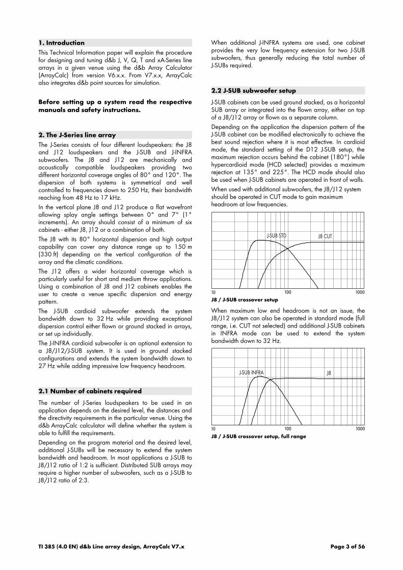
When used with additional subwoofers, the J8/J12 systemshould be operated in CUT mode to gain maximumheadroom at low frequencies.

J8 / J-SUB crossover setup

When maximum low end headroom is not an issue, theJ8/J12 system can also be operated in standard mode (fullrange, i.e. CUT not selected) and additional J-SUB cabinetsin INFRA mode can be used to extend the systembandwidth down to 32 Hz.

J8 / J-SUB crossover setup, full range


2.2.1 J-SUB ground stacks

Using J-SUB cabinets in L/R ground stacks providesmaximum system efficiency due to the ground coupling ofthe cabinets.

2.2.2 J-SUBs flown on top of a J8/J12 array

Flown J-SUBs create a more even level distribution overdistance. Compared to a ground stacked setup the area atthe very front below the arrays has much less low frequencylevel because of the longer distance to the subwoofers.However, when a high level of low frequency energy at thefront is desired, e.g. to compensate for a loud stage level,additional ground stacked subwoofers may be necessary.

2.2.3 Flown J-SUB columns

When complete columns of J-SUBs are flown the increasedvertical directivity adds to the distance effect describedabove and thus creates a longer throw of low frequencies.

Clever positioning of flown subwoofer columns behind themain and outfill arrays of TOP loudspeakers can greatlyenhance both visual appearance and acoustic performanceof the complete system through increased overall coherencebetween the different parts of the system.

2.2.4 J-SUB horizontal SUB array

Arranging J-SUBs in a horizontal array (SUB array)provides the most even horizontal coverage eliminating thecancellation zones to the left and right of the center of atypical L/R setup. Refer to section 8.8 on page 26.

2.3 J-SUB/J-INFRA subwoofer setup

When used with J-INFRA cabinets J-SUB subwoofers arealways operated in standard mode (i.e. INFRA notselected).

Depending on the application and the space requirementsa combination of J-SUB and J-INFRA cabinets can be set upin several different ways.

2.3.1 Combined J-INFRA/J-SUB ground stacks

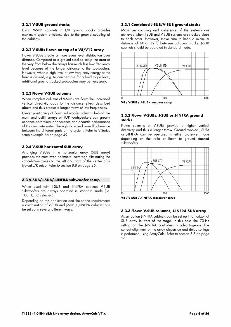
Maximum coupling and coherence of the systems areachieved when J-INFRA and J-SUB systems are stackedclose to each other. However, make sure to keep aminimum distance of 60 cm (2 ft) between adjacent stacks.J-INFRA cabinets should be operated in standard mode.

J8 / J-SUB / J-INFRA crossover setup

2.3.2 Flown J-SUB, J-INFRA ground stacks

Flown columns of J-SUBs provide a higher vertical directivityand thus a longer throw. Coupling with ground stackedJ-INFRAs will be less coherent and therefore requires the70 Hz setting on the J-INFRA controllers.

J8 / J-SUB / J-INFRA 70 Hz crossover setup

2.3.3 Flown J-SUB columns, J-INFRA SUB array

As an option J-INFRA cabinets can be set up in a horizontalSUB array in front of the stage. Also in this case the 70 Hzsetting on the J-INFRA controllers is advantageous. Thecorrect alignment of the array dispersion and delay settingsis performed using ArrayCalc. Refer to section 8.8 on page26.


3. The V-Series line array

The V-Series consists of three different loudspeakers: the V8and V12 loudspeakers and the V-SUB subwoofer. The V8and V12 are mechanically and acoustically compatibleloudspeakers providing two different horizontal coverageangles of 80° and 120°. The dispersion of both systems issymmetrical and well controlled to frequencies down to250 Hz, their bandwidth reaching from 65 Hz to 18 kHz.

In the vertical plane the V8 and V12 loudspeakers producea wavefront that allows splay angle settings ranging from0° to 14° (1° increments). An array should consist of aminimum of four cabinets - either V8, V12 or a combinationof both.

The V8 with its 80° horizontal dispersion and high outputcapability can cover any distance range up to 100 m(330 ft) depending on the vertical configuration of thearray and the climatic conditions.

The V12 offers a wider horizontal coverage which isparticularly useful for short and medium throw applications.Using a combination of V8 and V12 cabinets enables theuser to create a venue specific dispersion and energypattern.

The V-SUB cardioid subwoofer extends the systembandwidth down to 37 Hz while providing exceptionaldispersion control either in flown or ground stacked arraysor set up individually.

The J-INFRA cardioid subwoofer is an optional extension toa V8/V12/V-SUB system. It is used in ground stackedconfigurations and extends the system bandwidth down to27 Hz while adding impressive low frequency headroom.


The number of V-Series loudspeakers to be used in anapplication depends on the desired level, the distances andthe directivity requirements in the particular venue. Using thed&b ArrayCalc calculator will define whether the system isable to fulfill the requirements.

Depending on the program material and the desired level,additional V-SUBs will be necessary to extend the systembandwidth and headroom. In most applications a V-SUB toV8/V12 ratio of 1:2 is sufficient. Distributed SUB arraysmay require a higher number of subwoofers, such as aV-SUB to V8/V12 ratio of 2:3.

When additional J-INFRA systems are used, one cabinetprovides the very low frequency extension for two V-SUBsubwoofers, thus generally reducing the total number ofV-SUBs required.

3.2 V-SUB subwoofer setup

V-SUB cabinets can be used ground stacked, as ahorizontal SUB array or integrated into the flown array,either on top of a V8/V12 array or flown as a separatecolumn.

The V-SUB cabinet offers a cardioid dispersion patternthroughout its entire operating bandwidth.

When used with additional subwoofers, the V8/V12 systemshould be operated in CUT mode to gain maximumheadroom at low frequencies.

V8 / V-SUB crossover setup

When maximum low end headroom is not an issue, the V8/V12 system can also be operated in standard mode (fullrange, i.e. CUT not selected) and additional V-SUB cabinetsin 100 Hz mode or J-SUB cabinets in INFRA mode can beused to extend the system bandwidth down to38Hz/32 Hz.

V8 / V-SUB / J-SUB crossover setup, full range


3.2.1 V-SUB ground stacks

Using V-SUB cabinets in L/R ground stacks providesmaximum system efficiency due to the ground coupling ofthe cabinets.

3.2.2 V-SUBs flown on top of a V8/V12 array

Flown V-SUBs create a more even level distribution overdistance. Compared to a ground stacked setup the area atthe very front below the arrays has much less low frequencylevel because of the longer distance to the subwoofers.However, when a high level of low frequency energy at thefront is desired, e.g. to compensate for a loud stage level,additional ground stacked subwoofers may be necessary.

3.2.3 Flown V-SUB columns

When complete columns of V-SUBs are flown the increasedvertical directivity adds to the distance effect describedabove and thus creates a longer throw of low frequencies.

Clever positioning of flown subwoofer columns behind themain and outfill arrays of TOP loudspeakers can greatlyenhance both visual appearance and acoustic performanceof the complete system through increased overall coherencebetween the different parts of the system. Refer to V-Seriessetup example 6a on page 49.

3.2.4 V-SUB horizontal SUB array

Arranging V-SUBs in a horizontal array (SUB array)provides the most even horizontal coverage eliminating thecancellation zones to the left and right of the center of atypical L/R setup. Refer to section 8.8 on page 26.

3.3 V-SUB/J-SUB/J-INFRA subwoofer setup

When used with J-SUB and J-INFRA cabinets V-SUBsubwoofers are always operated in standard mode (i.e.100 Hz not selected).

Depending on the application and the space requirementsa combination of V-SUB and J-SUB / J-INFRA cabinets canbe set up in several different ways.

3.3.1 Combined J-SUB/V-SUB ground stacks

Maximum coupling and coherence of the systems areachieved when J-SUB and V-SUB systems are stacked closeto each other. However, make sure to keep a minimumdistance of 60 cm (2 ft) between adjacent stacks. J-SUBcabinets should be operated in standard mode.

V8 / V-SUB / J-SUB crossover setup

3.3.2 Flown V-SUBs, J-SUB or J-INFRA groundstacks

Flown columns of V-SUBs provide a higher verticaldirectivity and thus a longer throw. Ground stacked J-SUBsor J-INFRA can be operated in either crossover modedepending on the ratio of flown to ground stackedsubwoofers.

V8 / V-SUB / J-INFRA crossover setup

3.3.3 Flown V-SUB columns, J-INFRA SUB array

As an option J-INFRA cabinets can be set up in a horizontalSUB array in front of the stage. In this case the 70 Hzsetting on the J-INFRA controllers is advantageous. Thecorrect alignment of the array dispersion and delay settingsis performed using ArrayCalc. Refer to section 8.8 on page26.


4. The Q-Series line array

The Q1 is a compact and lightweight line array cabinetproviding a 75° constant directivity coverage in thehorizontal plane down to 400 Hz. The system can be usedfrom very small configurations of two cabinets per array upto a maximum of twenty cabinets per array for largervenues.

Q1 cabinets have a very low height of only 30 cm (1 ft)and when combined in arrays its accurate wavefront coversup to 14° vertically per cabinet, and couples coherently upto 12 kHz when configured in a straight (0° splay) longthrow section. The Q1 covers the frequency range from60 Hz to 17 kHz.

The Q7 and Q10 cabinets are mechanically andacoustically compatible loudspeakers with 75° x 40° and110° x 40° spherical dispersion patterns which can beused as a downfill (Q7) or nearfill extension with Q1arrays.

Smaller configurations of Q1 cabinets can also be usedground stacked, supported by Q-SUB cabinets. The mosteven energy distribution in the audience area will howeverbe achieved with a flown array.

The TI assumes that all Q-Series cabinets are driven by d&bD6 or D12 amplifiers. E-PAC amplifiers do not provide HFCand CSA settings.


The number of Q1 cabinets to be used in an applicationdepends on the desired level, the distances and thedirectivity requirements in the particular venue. Using thed&b ArrayCalc calculator will prove whether the system isable to fulfill the requirements.

Depending on the program material and the desired leveladditional Q-SUB subwoofer systems will be necessary toextend the system bandwidth and headroom. The numberof Q-SUBs needed per Q1 cabinet for serious full-rangeprogram will decrease with the size of the system. For smallsetups a 1:1 ratio is recommended, for example fourQ-SUBs to four Q1s, while larger systems will work with a2:3 ratio, for example eight Q-SUBs to twelve Q1s. Pleasenote that CSA setups require a multiple of three Q-SUBcabinets.

As an option Q1 systems can also be used with J-SUB orJ-INFRA subwoofers.

4.2 Subwoofer setup

Subwoofers are operated most efficiently when stacked onthe ground. For cleanest sound and coverage werecommend arranging subwoofers in a CSA configurationas described in d&b TI 330 Cardioid SUB array which isavailable for download from the d&b audiotechnik websiteat www.dbaudio.com.

When used with subwoofers, the Q1 systems should beoperated in CUT mode to gain maximum headroom at lowfrequencies.

Q-SUB (40 – 100/130 Hz)

Q-SUB cabinets can be used ground stacked or integratedinto the flown array, either on top of a Q1 array or flownas a separate column.

Flown Q-SUBs create a different level distribution in theaudience area than ground stacked ones. In particular thearea at the very front below the arrays has much less lowfrequency energy when subwoofers are included in thearray. This can be very useful in applications that do notrequire high levels of low frequency energy at the front,however for an event with high stage level additionalground stacked subwoofers may be necessary.

For Q1 arrays consisting of three or more cabinets werecommend the use of the 100 Hz setting for the Q-SUBsystems. Smaller Q1 arrays providing less coupling at lowfrequencies may benefit from the higher crossoverfrequency of the standard mode of the Q-SUBs (130 Hz).

Q1/Q-SUB crossover setup

Compared to a standard Q-SUB configuration a CSA setupproduces slightly less level above 70 Hz, so it may beadvantageous to use the standard (130 Hz) amplifiersetting.

J-SUB (32 – 70/100 Hz)

J-SUB cabinets can be used to supplement a Q1 system indifferent ways.

If the system is equipped with a sufficient number of Q-SUBcabinets, J-SUBs can be used to extend its bandwidth tobelow 32 Hz. Driven by D12 amplifiers set to INFRA modeone J-SUB will supplement up to four Q-SUB cabinets.

This combination will achieve its maximum headroom whenthe Q-SUBs are operated in the 130 Hz mode. If for audioreasons the lower crossover frequency to the Q1s is desiredyou may also reduce the gain of the Q-SUB amplifiers.Decreasing the gain by 2.5 dB will create the samedownward shift to the upper slope as switching to the100 Hz setting, but with less low frequency boost.

Q1/Q-SUB/J-SUB crossover setup


Please note that a combined ground stack consisting ofQ-SUB and J-SUB cabinets will only provide a consistentdirectivity when Q-SUBs are used in CSA setups. Also makesure to keep the required distance of 60 cm (2 ft) betweenthe stacks in order to not adversely affect the cardioiddirectivity of the systems.

J-SUB subwoofers can also be used as an alternative toground stacked Q-SUBs. In this case J-SUB cabinets areoperated in standard mode with a crossover frequency of100 Hz. One J-SUB will replace three Q-SUB cabinets in aCSA setup and extends the system bandwidth down to32 Hz.

Q1/J-SUB crossover setup

J-SUB cabinets in INFRA mode can be used to extend thebandwidth of a Q1 line array operated in full-range mode,without Q-SUBs. As this application does not expand theheadroom of the Q1 array it is only useful when mediumlevels but very low frequencies are required, for examplefor special effects.

Q1/J-SUB crossover setup, full range

J-INFRA (27 – 60/70 Hz)

To achieve the ultimate low frequency extension for a Qsystem consisting of Q1 and Q-SUB cabinets, additional J-INFRA subwoofers can be used. They provide a standard(60 Hz) and a 70 Hz mode. The selection of the modedepends on the coupling between J-INFRA and Q-SUBcabinets in the actual setup. When combined in a groundstack the standard (60 Hz) mode provides more headroomat very low frequencies.

Please note that a combined ground stack consisting ofQ-SUB and J-INFRA cabinets will only provide a consistentdirectivity when Q-SUBs are used in CSA setups. Also makesure to keep the required distance of 60 cm (2 ft) betweenthe stacks in order not to adversely affect the cardioiddirectivity of the systems.

Q1/Q-SUB/J-INFRA crossover setup


5. The T-Series line array

The T10 is a very compact loudspeaker system which canbe used both as a line array and as a high directivity pointsource speaker. For these applications the T10 cabinetprovides two different dispersion characteristics which canbe swapped over without any tools.

In line array mode the T10 provides a 105° constantdirectivity coverage in the horizontal plane allowing forvertical splay angles of up to 15° per cabinet. The systemcan be used from very small configurations of threecabinets per array up to a maximum of 20 cabinets perarray for larger venues. The T10 covers the frequencyrange from 68 Hz to 18 kHz.

The T-SUB subwoofer extends the system bandwidth downto 47 Hz either flown or ground stacked.

Smaller configurations of T10 cabinets can also be usedground stacked supported by T-SUB cabinets or mountedon a high stand. The most even energy distribution in theaudience area will however be achieved with a flownarray.


The number of T10 cabinets to be used in an applicationdepends on the desired level, the distances and thedirectivity requirements in the particular venue. Using thed&b ArrayCalc calculator will prove whether the system isable to fulfill the requirements.

Depending on the program material and the desired leveladditional T-SUB subwoofer systems will be necessary toextend the system bandwidth and headroom. The numberof T-SUBs needed per T10 cabinet for serious full-rangeprogram will decrease with the size of the system. For smallsetups a 1:3 ratio is recommended, for example one T-SUBto three T10s.

5.2 Subwoofer setup

When used with subwoofers, the T10 systems should beoperated in CUT mode to gain maximum headroom at lowfrequencies.

T-SUB (47 – 100/140 Hz)

T-SUB cabinets can be used to supplement the LF headroomof the T10 loudspeakers in various combinations. They canbe used ground stacked or integrated into the flown array,either on top of a T10 array or flown as a separate column.

Flown T-SUBs create a different level distribution in theaudience area than ground stacked ones. In particular thearea at the very front below the arrays has much less lowfrequency energy when subwoofers are included in thearray.

This can be very useful in applications that do not requirehigh levels of low frequency energy at the front, howeverfor an event requiring a loud stage level additional groundstacked subwoofers may be necessary.

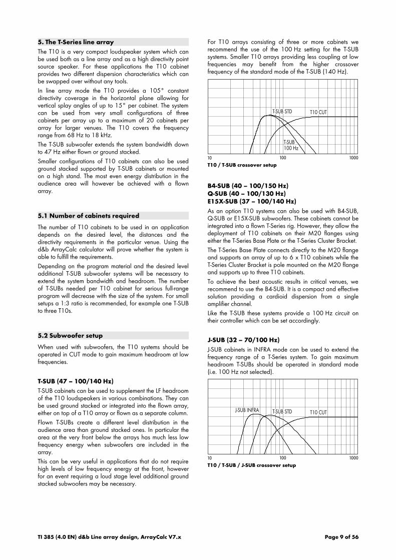
For T10 arrays consisting of three or more cabinets werecommend the use of the 100 Hz setting for the T-SUBsystems. Smaller T10 arrays providing less coupling at lowfrequencies may benefit from the higher crossoverfrequency of the standard mode of the T-SUB (140 Hz).

T10 / T-SUB crossover setup

B4-SUB (40 – 100/150 Hz)Q-SUB (40 – 100/130 Hz)E15X-SUB (37 – 100/140 Hz)

As an option T10 systems can also be used with B4-SUB,Q-SUB or E15X-SUB subwoofers. These cabinets cannot beintegrated into a flown T-Series rig. However, they allow thedeployment of T10 cabinets on their M20 flanges usingeither the T-Series Base Plate or the T-Series Cluster Bracket.

The T-Series Base Plate connects directly to the M20 flangeand supports an array of up to 6 x T10 cabinets while theT-Series Cluster Bracket is pole mounted on the M20 flangeand supports up to three T10 cabinets.

To achieve the best acoustic results in critical venues, werecommend to use the B4-SUB. It is a compact and effectivesolution providing a cardioid dispersion from a singleamplifier channel.

Like the T-SUB these systems provide a 100 Hz circuit ontheir controller which can be set accordingly.

J-SUB (32 – 70/100 Hz)

J-SUB cabinets in INFRA mode can be used to extend thefrequency range of a T-Series system. To gain maximumheadroom T-SUBs should be operated in standard mode(i.e. 100 Hz not selected).

T10 / T-SUB / J-SUB crossover setup


6. The xA-Series line array

The 10AL and 10AL-D line array modules of the xA-Serieshave been specifically designed for fixed installations withvisually unobtrusive integrated rigging systems.

For these applications, the cabinets are available with twodifferent constant directivity dispersion characteristics in thehorizontal plane:

The 10AL provides a 75° coverage while the 10AL-Dversion provides 105° of coverage. In the coupling plane,both allow for vertical splay angles of up to 15° percabinet. Both versions may be combined in one array, forexample with 10AL cabinets at the top for longer distancesand one or two 10AL-D to cover the areas near the stage.

Both systems can be used from small configurations of threecabinets per array up to a maximum of 9 cabinets perarray.

The 10AL (-D) covers the frequency range from 60 Hz to18 kHz. 18A-SUB or 27A-SUB subwoofers extend thesystem bandwidth down to 37 Hz or 40 Hz, respectively.They can be flown in a separate column, integrated at thetop or within an array or used as ground stackedapplications. When they are flown together with line arraymodules, the maximum number of total cabinets is reduceddue to the additional weight.

Configurations of up to six 10AL / 10AL-D cabinets canalso be used ground stacked, supported by 18S-SUB or27S-SUB cabinets. The most even energy distribution in theaudience area will however be achieved with a flownarray.


The number of 10AL or 10AL-D cabinets to be used in oneapplication depends on the desired level, the distances tobe covered and the directivity requirements of the particularvenue. Using the d&b ArrayCalc calculator will provewhether the system is able to fulfill the requirements.

Depending on the program material and the desired leveladditional 18A-SUB or 27A-SUB subwoofer systems maybe necessary to extend the system bandwidth andheadroom. The number of subwoofers required per 10AL(-D) cabinet to provide a serious full-range programdecreases with the size of the system. For small to mediumsize setups, a 1:3 ratio is recommended, for example one27A-SUB to three 10ALs.

6.2 Subwoofer setup

When used with subwoofers, the 10AL(-D) systems shouldbe operated in CUT mode to gain maximum headroom atlow frequencies.

27A-SUB/27S-SUB (40 – 100/140 Hz)

Subwoofers can be used to supplement the LF headroom ofthe 10AL loudspeakers in various combinations.

To achieve the best acoustic result in critical venues, werecommend the use of 27A-SUB or 27S-SUB subwoofers.They offer a compact and effective solution by providingcardioid dispersion from a single amplifier channel.

They can be used ground stacked (27S-SUB and 27A-SUB)or integrated into the flown array (27A-SUB), either at thetop or within a 10AL array, or flown as a separate column.

Flown subwoofers create a different level distribution in theaudience area than ground stacked ones. Particularly thearea directly at the front below the arrays provides less lowfrequency energy when subwoofers are included in thearray.

This can be very useful in applications that do not requirehigh levels of low frequency energy at the front, howeverfor an event requiring a loud stage level, additional groundstacked subwoofers may be necessary.

For 10AL arrays consisting of three or more cabinets, werecommend the use of the 100 Hz setting for thesubwoofers. Smaller 10AL arrays providing less coupling atlow frequencies may benefit from the higher crossoverfrequency of the standard mode (140 Hz).

10AL / 18A/27A-SUB crossover setup

18A-SUB/18S-SUB (37 – 100/140 Hz)

18A-SUB or 18S-SUB cabinets can be used in the sameway as 27A-SUB or 27S-SUB cabinets but without thebenefit of cardioid dispersion.

For these systems, just like for the 27S/A-SUBs, a 100 Hzcircuit is available on the controller, which can be setaccordingly.


7. The d&b point sources

From Version V7x.x, a range of d&b point sourceloudspeakers is available for integration into a project. Thisoption mainly allows you to use all top cabinets of theWhite Range xS-Series both in stand-alone projects and incombination with 10AL arrays, for example. In addition, arange of point source loudspeakers of the d&b Black Rangecan be selected, for example all current top cabinets of theE-Series, Q(i)7, Q(i)1 and T(i)10PS. Apart from that, aT(i)10L loudspeaker that is deployed horizontally may alsobe used as a single nearfill with the T10PS setup althoughits polar dispersion does not reflect a "point source".

For cabinets that are equipped with rotatable HF horns,both horn orientations can be selected separately. Eachselectable orientation for a specific loudspeaker type usesits own measured polar data set. This is defined by thechosen nominal horizontal and vertical dispersion anglesand follows the convention [SystemName] [horizontaldispersion] x [vertical dispersion] while the cabinet itselfremains in its typical mechanical orientation, i.e. in anupright position (e.g. 10S 75x50; E6 55x100; Q7 40x75etc).

If a system is used lying on its side, the standard datasetmust be used and the cabinet rotation must be set to either90°(on its left side, seen from a listener's position) or 270°(on its right side, seen from a listener's position). The cabinetcan be rotated in steps of 90° degrees. Each individualcabinet can be freely positioned within the room withhorizontal or vertical aiming.

Selecting a loudspeaker optionally displays a balloon polarplot or its vertical aiming into the room.

More specific loudspeaker data can be found in therelevant documentation of d&b White and Black Rangeproducts.


The number of point source cabinets is primarily defined bytheir specific application, for example as nearfill or delaysystems or as the main system. Of course, the number ofcabinets also depends on the desired level, the distances tobe covered and the directivity requirements in the particularvenue or project. Using the d&b ArrayCalc calculator willprove whether the system is able to fulfill the specificrequirements.

Depending on the program material and the desired level,additional d&b subwoofer systems may be necessary toextend the bandwidth and headroom

When used with subwoofers, the point sources should beoperated in CUT mode to gain maximum headroom at lowfrequencies.


8. ArrayCalc

For both acoustic and safety reasons all d&b line arraysmust be designed using the d&b ArrayCalc simulation tool.

ArrayCalc also provides functionality to integrate individuald&b point source loudspeakers into a simulation project.ArrayCalc is available for PC and MAC.ArrayCalc uses a sophisticated mathematical modelsynthesizing each line-array cabinet's wavefront with anarray of narrowly spaced point sources combined withmeasured high-resolution dispersion data. Sound pressurelevel is calculated in 3D using complex data (vectorsummation).Point sources are modelled using complex measured high-resolution 3D polar data.

ArrayCalc provides the following features:

— Level distribution on up to five different audience areasdisplayed in 3D format for selectable frequency bandsfrom 32 Hz to 12.5 kHz.

— Calculation of absolute sound pressure levels inaudience areas including system headroom supervisionfor different input signals.

— Combination of up to 14 different array pairs distributedacross the venue plus ground stacked subwoofers in L/Rcombinations or arranged as SUB array.

— Flown subwoofers integrated into the line arrays or flownas separate columns.

— Additional integration of up to six groups of d&b pointsource loudspeakers.

— Auto tuning algorithms for vertical aiming and splayangles of arrays as well as SUB array settings.

— Tuning of all relevant amplifier settings like level, arraycoupling, crossover and cardioid modes.

— Simulation of air absorption effects depending onenvironmental conditions, tuning of the respectiveamplifier settings.

— System time alignment between different sources andsubwoofers using impulse and phase response data.

— Calculation of load and space requirements for riggingpoints.

— Calculation and supervision of electronic and physicalload conditions as well as mechanical forces withinarrays.

— Design and calculation printouts, printable parts lists forinventory control and loading as well as DXF and EASEexport functions.

— Project file export into the d&b R1 Remote controlsoftware.

System requirements

— PC with Intel/AMD (1 GHz or more); WindowsXP SP2 / Vista / 7.

— or Macintosh (Power PC or Intel); Mac OS 10.5 orhigher.

— 512 MB RAM, 2 GB recommended.

— 25 MB of available hard disk capacity.

— Mouse, preferably with wheel.

— Minimum screen resolution 1280 x 1024; on smallerscreens viewport has to be scrolled.

8.1 ArrayCalc installation

Windows systems:To install ArrayCalc, start ArrayCalcSetup.exe orArrayCalcSetup.msi and follow the instructions in the setupdialog.

The default installation path is:

C:\Program files\dbaudio\ArrayCalc

A default project directory will be created:

Windows XP: C:\Documents and settings\'username'\My Documents\dbaudio

Windows 7:C:\Users\'username'\My Documents\dbaudio

To remove ArrayCalc from your system, go to Start –Settings – Control Panel – Add or remove programs in theControl Panel folder.

Select the ArrayCalc entry from the list and click theRemove button. The uninstall routine starts and the softwareis removed including all related components.

Macintosh systems:Double-click ArrayCalc.dmg and drag ArrayCalc to yourapplications folder.

To remove ArrayCalc from your system, move ArrayCalcinto the trash bin.


8.2 Starting ArrayCalc

Windows:ArrayCalc can either be started via the Windows StartMenu, where it will appear in Programs – dbaudio –ArrayCalc – ArrayCalc or by double-clicking the ArrayCalcdesktop icon.

Windows automatically links ArrayCalc project files(*.dbac) to ArrayCalc. Alternatively, the program cantherefore be started by double-clicking on any ArrayCalcproject file.

Macintosh:Click ArrayCalc or any ArrayCalc project file.

8.3 ArrayCalc menu options and Toolbar

The drop-down menus "File", "View", "Sources","Extras" and"Help" on top of the page provide access to additionalfunctions of ArrayCalc. Several menu items can also beaccessed directly by clicking the respective button in thetoolbar underneath.

8.3.1 File menu

— New: Creates a new project by loading the defaultsetup. Modifying a simple existing setup is usually muchfaster than starting without any data.

— Open / Save / Save as: Loads or saves the projectdata including room data, arrays, SUB array design andalignment settings from/to a file. (file format: *.dbac).

It is possible to open setup files created with ArrayCalcversion 5.x, however additional data has to be providedmanually. Opening setups from earlier Microsoft Excelbased versions of ArrayCalc is not possible.

— Open recent project: Provides direct access to thelast six projects saved.

— Open example project: Provides direct access tothe example project files included in the installationpackage.

— Export DXF: Exports all / the currently selected arrayor the SUB array to a *.dxf graphics file.

— Export EASE: Exports the selected array to a *.txt filewhich can be imported by the d&b LineArray dll forEASE 4.x.

— Export PNG: Only available from the 3D plot page;exports the 3D plot, the color scale and the underlyingsignal selection to a *.png file.

— Print: Print options for several pages of ArrayCalc.

— Print preview: Provides access to a print preview withseveral options (depending on the printer selected).

— New instance: Opens another instance of ArrayCalc.

— Exit: Closes d&b ArrayCalc.

8.3.2 View menu

— Toolbar: Allows the toolbar to be switched on/off.

— Status bar: Allows the status bar to be switchedon/off.

8.3.3 Sources menu

When working on the Sources page, the Sources menuprovides the following functions:

— Add array: Adds a new empty array to the project.The maximum number of arrays is fourteen.

— Auto splay: Provides starting values for the splayangles of the selected array.

— Add point sources: Adds a new empty point sourcedialog to the project. The maximum number of pointsource groups is six. Each group may consist of up to 14single point sources.

— Rename: Highlights the name of the selected sourcefor editing.

— Copy: Creates a copy of the selected source settings inthe internal clipboard.

— Paste: Pastes all source settings copied to the internalclipboard into the selected source.

— Paste as new: Creates a new source containing allsettings from the internal clipboard.

— Delete: Deletes the selected source from the projectafter confirmation.

— Export source: Exports the settings of the selectedsource to an ArrayCalc description file (*.dbea forarrays, *.dbep for groups of point sources).

— Import source: Imports the settings of a source froman ArrayCalc description file (*.dbea for arrays, *.dbepfor groups of point sources) to the selected source.

8.3.4 Extras / Options menu

— Units: Provides access to the selection of:

the measurement units: metric (m/kg) or imperial (ft/lbs).

the temperature units: degrees centigrade (° C) orFahrenheit (° F).

— Web search: Provides access to automatic updateoptions.

— Graphics: Provides optional color palette for brightenvironment.

— R1 export: Defines the start mode of the generated R1file.

8.3.5 Help menu

— F1 Help: Provides access to this document (TI 385).

— Web search: Searches the web for updates.

— System info: Provides information on the computersystem.

— About: Provides information on the version ofArrayCalc you are using.


8.4 ArrayCalc workspace

The workspace is sub-divided into seven pages givingaccess to the various data input tables and calculationresults:

The usual procedure is first to enter the project descriptionand room data on the Sources page (see following section).On the Sources page you can design a line array profiledepending on the vertical dispersion requirements for eachposition. In addition, or alternatively, you can define andenter a group of d&b point sources. Furthermore anoptional SUB array can be defined and tuned here (seealso section 8.8 SUB arrays on page 26).If you use more than one source, the Alignment page (seesection 8.9 Alignment page on page 32) helps you tocorrectly time align the sources in a next step. This alsoincludes the SUB array alignment.In a third step, the 3D plot page enables you to tune andverify the detailed settings of the horizontal aiming andrelative leveling of the arrays in order to achieve the desiredlevel distribution.

8.5 Sources page

Line arrays dialog

8.5.1 General data input

Cells with a gray background accept direct data input.

A single click places the cursor in the cell to edit data.

A double-click additionally highlights the value left of thedecimal point for editing and replacement while a tripleclick highlights the entire cell contents for editing andreplacement.

To switch between metric and imperial units, refer to section8.3 ArrayCalc menu options on page 13.

Cells with a drop-down icon attached offer a predefinedselection of data input available from the drop-down list.

Place the mouse pointer onto these cells and turn the mousewheel to scroll through the possible selections for therespective cell.

This is a fast tool to manually set splay angles.

8.5.2 Project settings

Project settings dialog

Enter information about the project you are planning. Thisdata will be displayed in the headline or in the dedicatedComments sections as well as in the printouts.

8.5.3 Room settings

Room settings dialog


Listening planes:

Up to 5 main listening areas can be defined. Each plane isactivated by its on/off toggle switch.

When set to on, the gray cells of the respective listeningarea accept direct data input.

To approximate an arena type venue, planes 2 to 5 can beextended at their left and right sides towards the stagefront. The width of the respective plane has to increase fromfront to back.

Switch on the P2-P5 Sides to activate and enter the desiredextension in the x-direction.

Enter the coordinates of the listening planes and the typicalheight of the listener's ear.

Transparent option:

When a sound from a source hits a plane, it gets absorbedby the plane. This is indicated by the fact that the mainbeams of the relevant cabinets end as soon as they hit theplane. Listening points on other planes without a direct lineof sight to a source or points which are in the shadow of aparticular plane do not receive any sound from the source.This feature can be specifically helpful when simulating thelevel of under balcony listening positions.

When a plane's Transparent switch is enabled, the planewill not absorb the sound. In this case, the beams will go"through" the plane onto any other planes that are locatedin its shadow.

When the planes are set to absorbent, the system checksevery single listening point for an acoustic "sightline",something which requires a considerable amount ofcomputing time. As a result, to speed up calculation,listening planes should be switched to Transparent unlessthe planes need to be absorbent to check the levels underbalconies, etc. For this reason, in every new project the“Transparent” option is enabled as default.

Obstacles:

Up to two obstacles (screens, displays, etc.) can bedefined. Each obstacle is activated by its on/off toggleswitch. When set to on, the gray cells of the respectiveobstacle accept direct data input.

In the first row named "Position" the x/y center coordinatesof the obstacle are defined, as well as either its top orbottom height (z) and a possible rotation angle in the x-yplane. In the second row named "Dimensions" its extensionin x/y/z direction is defined. The x/y dimensions have tobe positive values, while z can be positive or negativedepending on whether the obstacle extends upward ordownward from the height (z) position.

Obstacles are shown in the Top view diagram and in the3D plot.

As far as acoustic transparency is concerned, obstaclesshow the same behavior as described above for thelistening planes.

When the Pair option is enabled, a second obstacle isgenerated using the mirrored value of the y coordinate ofthe first obstacle.

8.5.4 Deleting and adding sources

You can create up to 14 individual arrays or symmetricalpairs of arrays and in addition six groups of point sourcesby clicking the "Add array" or the "Add point sources"button in the toolbar or by selecting the "Add array"/"Addpoint sources" item from the Sources menu. For each linearray or point source group in the project, a separatesettings dialog is created and available for use.

You can delete the sources open for editing by clicking the"Delete" button in the toolbar or by selecting the "Delete"item from the Sources menu. This action has to be confirmedand can be canceled again before final execution.

8.6 Line Arrays

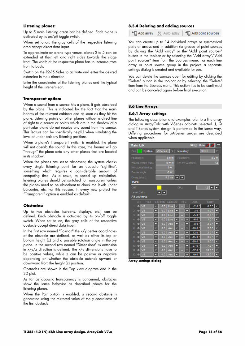
8.6.1 Array settings

The following description and examples refer to a line arraydialog in ArrayCalc with V-Series cabinets selected. J, Qand T-Series system design is performed in the same way.Differing procedures for xA-Series arrays are describedwhen applicable.

Array settings dialog


Renaming arrays

In each headline of the array settings dialogs, the name ofthe respective array can be edited directly by clicking onthe text at the left.

The headline also contains a Gain Reduction LED (GR LED)and individual Mute switches for the entire array(s). Theirfunctions are described in detail in sections 8.6.3 GainReduction indicator GR on page 21 and section 8.6.9Maximum SPL and headroom on page 21.ArrayCalc supports different array setups including flownsubwoofers or ground stacked configurations. The type ofsystem and its mounting can be selected independently foreach array / pair of arrays.

Selection of system and mounting

Array positions, aiming and No. of cabinets

Position x / Position y

Defines the coordinates of the top front of the array. Whenthe Pair option is enabled, the y coordinate is always set toa positive value and the second array will be located at thenegative y value.

Frame height front

Height above ground of the top front edge of the Flyingframe (trim height).

Horizontal aiming

Horizontal aiming of the array. Positive angle: aimedtowards positive y values. (For pairs of arrays it refers to thehouse left array, i.e. positive value: rotated inwards,negative value: outwards). To calculate SPL over distance,ArrayCalc uses the projection of the listening planes in thedirection of each array´s horizontal aiming.

Frame angle

Sets the vertical aiming of the entire array. The verticalorientation of the uppermost cabinet is identical to the frameangle.

A line array produces a precisely shaped wavefrontfollowing the mechanical arrangement of the cabinets. Thecut off at the upper and lower limits of the verticaldispersion of a column is very sharp, and therefore accurateaiming is absolutely essential to address the desiredaudience area.

The first parameter to set is the flying frame angle and

height. For best results the top cabinet of the column shouldaim at the farthest point in the audience area. Aiming theFlying frame up to 2° above this point sometimes gives asmoother coverage and can help to stabilize the leveldistribution under changing climatic conditions outdoors.

Check the SPL plot for the effect but at the same timeconsider a possible increase of reflections from the rearwalls.

No. of cabinets

Total number of SUB and TOP cabinets used in the array.The final selection of the cabinet type for each individualposition is made in the cabinets section.

With Q1 arrays a Q7 loudspeaker can be inserted at thevery bottom of the column (horizontally mounted withrotated horn). The maximum splay of 14° is used here.Compared to a Q1 used in the same position this setupgains about 10° more coverage to the front for highfrequencies. The Q7 has to be driven by a separateamplifier channel in Q7 configuration.

xA-Series: No. of cabinets / TOP cabinetorientation

In an xA-Series array, SUBsand TOPs may be arrangedin any order within thearray.

The TOPs of the xA-Series have a biaxial design. Althoughthey do not provide mechanical symmetry, their dispersiondesign is highly symmetrical within the nominal dispersionarea, the level roll-off beyond that area is inevitably notperfectly symmetrical. To enable a symmetrical setup forstereo systems, the cabinet orientation may be reversed. Inthe default orientation, the HF waveguide is located to theleft, viewed from the audience side.

Array group controls

Depending on the selected array and the cabinet typesused, group controls are available which define the mainamplifier settings for the whole array or functional parts ofit. The simulation result changes in accordance with thesettings.

General group controls

Mute: Located in the headline in order to be availableeven if the array is not opened for editing. Depending onthe setting of the Mute switch, an array will be taken intoaccount in the 3D mapping and be displayed, or notdisplayed, on the Alignment page. The Level vs. distanceresult of the individual array is not affected by the Mutesetting.


Delay value for the array: Acts as an absolutecontrol, i.e. the value entered here will be set for eachloudspeaker of the array.

Loudspeaker specific amplifier controls

Level control: Independent level controls for SUBs andTOPs each working with relative values to maintainindividual tunings.

CUT: Available for all line array TOP speakers. Reducesthe low frequency level. To be selected depending on thesubwoofer setup.

CPL: Available for all line array speakers. Reduces the lowand mid frequency level. The setting depends on the arraylength and curvature.

HFC: Available for all line array speakers. Increases highfrequency response to compensate for air absorptioneffects. HFC can only be set when the “air absorption”switch is activated.

HCD: Available for active cardioid J-SUB and J-INFRAsubwoofers. Changes from cardioid to hypercardioid mode.

INFRA, 100 Hz, 70 Hz: Subwoofer crossover optionsfor different models.

Line array configuration settings, Levels andSplay angles

You can define the amplifier settings for each cabinetindividually. However, if two or more cabinets are linked tothe same amplifier or amplifier channels, identical settingshave to be chosen for these cabinets.

The coverage and level distribution in the audience areasare mainly adjusted using the splay angles between thecabinets. The first entry in the column is the angle betweenthe Flying frame and the first cabinet which is always set to0°. Left to the splay column the absolute vertical aiming ofeach cabinet is indicated.

The J8/J12 wavefront characteristic allows a maximumsplay angle between adjacent cabinets of 7° while stillproviding a gapless coverage at high frequencies(V8/V12: 14°; Q1: 14°; T10: 15°). Lower frequencieswill disperse into a wider area creating an overlap of thecoverage patterns between the single cabinets. Thereforedirectivity and the level of lower frequencies increases withevery cabinet added to the column.

Decreasing the splay angles will enforce the overlap of thecoverage patterns at high frequencies resulting in increaseddirectivity and high-frequency output.

Small splay angles are used when covering remoteaudience areas where additional high-frequency energy isneeded to maintain intelligibility in a reverberant venue,and to compensate for the HF absorption of air whichincreases with distance.

Usually the distances to the audience that an array has tocover decrease from the top to the bottom of a column,consequently it is desirable to gradually increase thevertical splay angles between adjacent cabinets, resulting ina spiral -or "J"-shape.

If a desired level distribution cannot be achieved with agiven number of cabinets and/or external restrictions in theplacement of the array, the levels of individual cabinets canbe modified. This should always be the last option, andgenerally be limited to a few dBs.

Line / Arc selection

Depending on the array curvature in the respective sectionof the array, you can select an appropriate configuration.The Arc (Q1: standard) configuration is applied when thespeakers are used in a curved array section while the Lineconfiguration is used for groups of four or more speakersclosely coupled with small splay angles to form a longthrow array section. Refer to section 9.1 Arc and Lineconfigurations on page 40 for further details.

HFC settings

With the calculation for excessive absorption of highfrequencies in air enabled, the selectors for the HFCcompensation circuit will be available and its setting will beincluded in the calculation. When the air absorptioncalculation is globally switched off, the processing for "HFCoff" will be taken into account. By globally switching the airabsorption calculation on/off, a meaningful compensationof the individual amplifier channels can be verified. Refer tosection for further details.

8.6.2 Auto Splay

For line array design you may use the "Auto splay" functionlocated in the tool bar (or in the Sources menu) to get startvalues which should later be optimized manually to achievethe desired SPL distribution.

The algorithm's first criterion attempts to fully cover theactivated listening planes. If more total splay is availablethan needed for coverage, a progressively splayed arraywith cabinet aiming points equally spaced along thelistening planes is created. The Flying frame angle (= topcabinet) will be aimed at the farthest listening point.

If the Auto Splay function proposes a set of large splayangles, only slightly increasing from top to bottom, this is agood indication that more cabinets should be consideredfor the application.


8.6.3 Copy, Paste, Paste as new

— Copy: Creates a copy of the selected array or groupsof sources with all settings in the internal clipboard.

— Paste: Pastes all source settings copied to the internalclipboard into the selected array or group of sources.

— Paste as new: Creates a new array or group ofsources containing all settings from the internalclipboard.

Gain Reduction indicator GR

Each cabinet has a yellow GR LED which indicates when aparticular amplifier channel has reached its limit for thegiven signal level with one of the simulated input signalsselected for the 2D and 3D SPL plots.

A possible Gain Reduction is not considered in the SPLcalculations, i.e. will not limit a cabinet´s calculated outputand will therefore not modify the SPL distribution.Consequently, with (too) many GR LEDs on, the calculatedand displayed level distribution might actually not beattainable.

Whenever a GR LED lights up for a cabinet within an array,the GR LED in the headline is activated even if the array isnot opened for editing.

Renaming sources

In each headline of the array settings dialogs, the name ofthe respective array or group of sources can be editeddirectly by clicking on the text at the left.

The headline also contains a Gain Reduction LED (GR LED)and individual Mute buttons for the entire array(s). Theirfunctions are described in detail in sections 8.6.3 GainReduction indicator GR on page 21 and section 8.6.9Maximum SPL and headroom on page 21.The type ofsystem and its mounting can be selected independently foreach source / pair of sources.

8.6.4 Mechanical Load conditions for arrays

WARNING!

Potential risk of personal injury and/ordamage to materials.

Never set up an array which exceeds the load limits.

— Reduce the number of cabinets or the total splay angleuntil the load conditions are within limits.

When a given array configuration exceeds the mechanicalload limits, a warning is displayed in the array´s headline:

Exceeding the BGV-C1 limits will bring up a yellow warningsymbol:

Exceeding the absolute load limits will bring up a redwarning symbol:

Array selection

You can select any array defined in the project for displayand simulation by opening the respective array settingsdialog.

Load conditions for selected array

Load conditions and single pick point settings

This section provides general information on the mechanicalload conditions of the array:

If the load conditions are within the load limits, the followingmessage will be displayed:

For applications covered by the BGV C1 Rule for thePrevention of Accidents, "within BGV-C1 limits" is displayedas additional information if the designed array fulfills theload requirements.


If the load limits are exceeded, the following message willbe displayed:

For applications covered by the BGV C1 Rule for thePrevention of Accidents, "out off BGV-C1 limits" is displayedas additional information if the designed array exceeds theload requirements.

Load conditions for xA-Series arrays

Since xA-Series arrays are intended for fixed installation useonly, the additional requirements of the BGV C1 rules donot apply. Consequently, no further details are providedhere.

Some xA-Series configurations would exceed the riggingsystem load capacity if the fully assembled array was liftedfrom horizontal assembly position (i.e. when the array wasassembled on the floor):

In this case, the array must be assembled vertically. Addonly one cabinet to the suspended array at a time.

Total mass

The calculated weight of the array including all riggingcomponents.

Single pickpt. hole no/pos

For single hoist operation, these values indicate where theLoad adapter should be attached to the Flying frame to getthe desired vertical aiming of the array.

The closest hole of the frame's hole grid, counted from thefront of the frame, as well as the exact position as adistance from the front of the frame's center beam aredisplayed.

The J Load adapter supplied with the J Flying frame allowsthe pick point position to be set with a resolution of a 1/2hole. The Q and T-Series Flying frames with Q/T Loadadapter provide a resolution of 1/4 hole.

If the calculated pick point is beyond the frame, an errormessage will be displayed:

Single hoist operation might not be allowed for largearrays. In this case these cells show "--".

Height of lowest edge

Height above the ground of the lowest edge of the array.Allows easy verification of trim height using a laser rangefinder or a tape measure.

V and Q Flying adapter

If a small V or Q-Series array allows the optional use of theZ5385 V Flying adapter / Z5156 Q Flying adapter, thepickpoint information is displayed on the Rigging plot pageprovided the corresponding array is selected on this page.Refer to section 8.13 Rigging plot page on page 38.

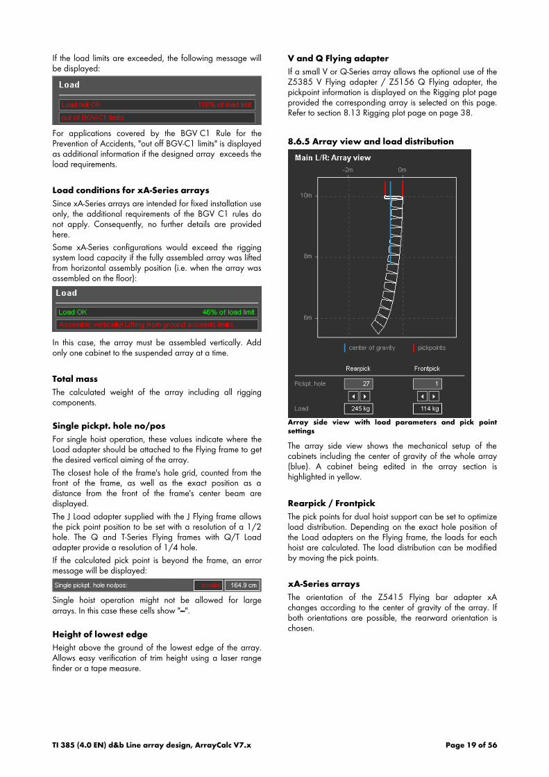
8.6.5 Array view and load distribution

Array side view with load parameters and pick pointsettings

The array side view shows the mechanical setup of thecabinets including the center of gravity of the whole array(blue). A cabinet being edited in the array section ishighlighted in yellow.

Rearpick / Frontpick

The pick points for dual hoist support can be set to optimizeload distribution. Depending on the exact hole position ofthe Load adapters on the Flying frame, the loads for eachhoist are calculated. The load distribution can be modifiedby moving the pick points.

xA-Series arrays

The orientation of the Z5415 Flying bar adapter xAchanges according to the center of gravity of the array. Ifboth orientations are possible, the rearward orientation ischosen.


8.6.6 Top view diagram for arrays

Top view of listening planes and arrays

The top view shows the active listening planes, the positionof the arrays and their horizontal coverage area (nominal –6 dB isobars).

All arrays of a project are shown, the currently selected oneis colored, all others are shown in gray. The dashed beamsindicate the main axis of each array, the yellow (gray)dotted lines the coverage area of the uppermost cabinetand the orange (gray) dotted lines the lowest cabinet, inthis case a J12. The coverage lines end when they hit alistening plane that is set to absorbent. (See section 8.5.3Listening planes on page 15).

8.6.7 Profile at array aiming

Profile view at horizontal aiming of selected array

The profile view shows a cross section through the activelistening planes in the direction of the selected array's mainaxis with the listener ear height indicated. The x-scaling isalways relative to the array's position and therefore doesnot necessarily correspond to the absolute scaling of thetop view diagram. Each dashed beam marks the main axisof one cabinet. The beam of a cabinet being edited in thearray section is highlighted in yellow.

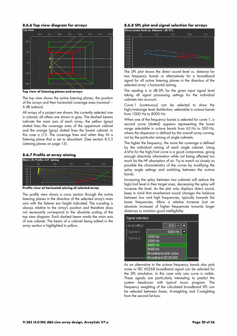
8.6.8 SPL plot and signal selection for arrays

The SPL plot shows the direct sound level vs. distance fortwo frequency bands or alternatively for a broadbandsignal for all active listening planes in the direction of theselected array´s horizontal aiming.

The reading is in dB SPL for the given input signal leveltaking all signal processing settings for the individualcabinets into account.

Curve 1 (continuous) can be selected to show thehigh/midrange level distribution, selectable in octave bandsfrom 1000 Hz to 8000 Hz.

When one of the frequency bands is selected for curve 1, asecond curve (dotted) appears representing the lowerrange selectable in octave bands from 63 Hz to 500 Hz,where the dispersion is defined by the overall array curving,not by the particular aiming of single cabinets.

The higher the frequency, the more the coverage is definedby the individual aiming of each single cabinet. Using4 kHz for the high/mid curve is a good compromise, givingenough directivity information while not being affected toomuch by the HF absorption of air. Try to match as closely aspossible the characteristics of the curves by modifying thesplay angle settings and switching between the octavebands.

Increasing the splay between two cabinets will reduce thehigh/mid level in their target area, decreasing the splay willincrease the level. As the plot only displays direct sound,keep in mind that reverberant sound changes the balancebetween low and high frequencies, typically towards thelower frequencies. Allow a relative increase (not anabsolute increase) of higher frequencies towards largerdistances to maintain good intelligibility.

As an alternative to the octave frequency bands also pinknoise or IEC 60268 broadband signal can be selected forthe SPL simulation. In this case only one curve is visible.These signals are particularly interesting to predict thesystem headroom with typical music program. Thefrequency weighting of the calculated broadband SPL canbe selected between linear, A-weighting and C-weightingfrom the second list box.


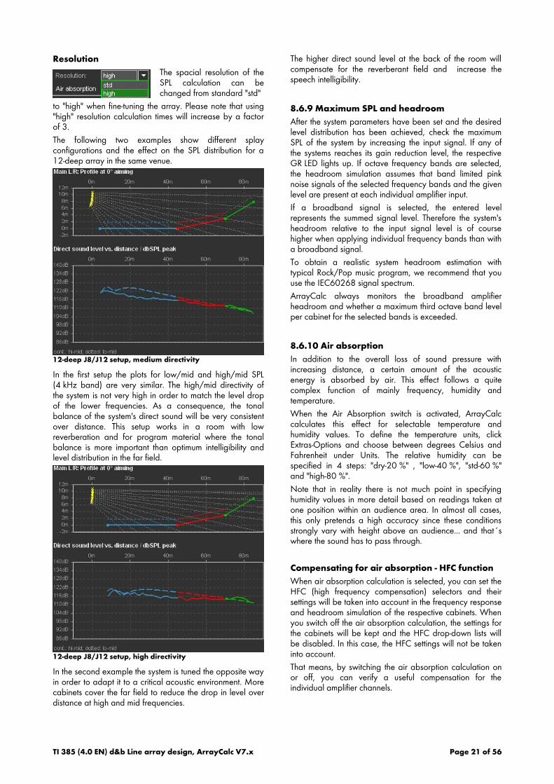
Resolution

The spacial resolution of theSPL calculation can bechanged from standard "std"

to "high" when fine-tuning the array. Please note that using"high" resolution calculation times will increase by a factorof 3.

The following two examples show different splayconfigurations and the effect on the SPL distribution for a12-deep array in the same venue.

12-deep J8/J12 setup, medium directivity

In the first setup the plots for low/mid and high/mid SPL(4 kHz band) are very similar. The high/mid directivity ofthe system is not very high in order to match the level dropof the lower frequencies. As a consequence, the tonalbalance of the system's direct sound will be very consistentover distance. This setup works in a room with lowreverberation and for program material where the tonalbalance is more important than optimum intelligibility andlevel distribution in the far field.

12-deep J8/J12 setup, high directivity

In the second example the system is tuned the opposite wayin order to adapt it to a critical acoustic environment. Morecabinets cover the far field to reduce the drop in level overdistance at high and mid frequencies.

The higher direct sound level at the back of the room willcompensate for the reverberant field and increase thespeech intelligibility.

8.6.9 Maximum SPL and headroom

After the system parameters have been set and the desiredlevel distribution has been achieved, check the maximumSPL of the system by increasing the input signal. If any ofthe systems reaches its gain reduction level, the respectiveGR LED lights up. If octave frequency bands are selected,the headroom simulation assumes that band limited pinknoise signals of the selected frequency bands and the givenlevel are present at each individual amplifier input.

If a broadband signal is selected, the entered levelrepresents the summed signal level. Therefore the system'sheadroom relative to the input signal level is of coursehigher when applying individual frequency bands than witha broadband signal.

To obtain a realistic system headroom estimation withtypical Rock/Pop music program, we recommend that youuse the IEC60268 signal spectrum.

ArrayCalc always monitors the broadband amplifierheadroom and whether a maximum third octave band levelper cabinet for the selected bands is exceeded.

8.6.10 Air absorption

In addition to the overall loss of sound pressure withincreasing distance, a certain amount of the acousticenergy is absorbed by air. This effect follows a quitecomplex function of mainly frequency, humidity andtemperature.

When the Air Absorption switch is activated, ArrayCalccalculates this effect for selectable temperature andhumidity values. To define the temperature units, clickExtras-Options and choose between degrees Celsius andFahrenheit under Units. The relative humidity can bespecified in 4 steps: "dry-20 %" , "low-40 %", "std-60 %"and "high-80 %".

Note that in reality there is not much point in specifyinghumidity values in more detail based on readings taken atone position within an audience area. In almost all cases,this only pretends a high accuracy since these conditionsstrongly vary with height above an audience... and that´swhere the sound has to pass through.

Compensating for air absorption - HFC function

When air absorption calculation is selected, you can set theHFC (high frequency compensation) selectors and theirsettings will be taken into account in the frequency responseand headroom simulation of the respective cabinets. Whenyou switch off the air absorption calculation, the settings forthe cabinets will be kept and the HFC drop-down lists willbe disabled. In this case, the HFC settings will not be takeninto account.

That means, by switching the air absorption calculation onor off, you can verify a useful compensation for theindividual amplifier channels.


The different settings of the HFC correction cover thefollowing distances according to the individual systemsused:

Series HFC1 HFC2

J 40 m 80 m

V 30 m 60 m

Q 30 m --

T 25 m 50 m

xA 25 m 50 m

Overview of HFC distance compensation

The values apply for a relative humidity of 40 %. The HFC2compensation in the J8/J12 Line, V8/V12 Line and T10Line setups includes a bandwidth limitation to approx.10 kHz to keep the necessary boost within meaningful limitsnot wasting the system's headroom.

See also section 8.6.10 Air absorption on page 21 forfurther details.

8.6.11 Array EQ / CPL

Six J8/J12 cabinets arrayed vertically with up to 12° totalsplay angle produce a flat frequency response. Longercolumns with more total splay will boost low and low/midfrequencies. The adjustable CPL function in the amplifiercompensates for these effects. While setting the splayangles the Array EQ "Coupling" parameter (CPL, 0...–9 dB)can be set to a useful attenuation of lower frequencies toachieve a balanced sound. The setting of the CPLparameter affects the frequency response of the array, thecurves of the SPL plot shifting accordingly.

The same principle applies to Q and T arrays. CPL shouldbe used with arrays of four or more cabinets and a totalsplay of more than 15°.

Matching the 500 Hz curve (selectable for the Lo-midcurve) with the 1000 Hz curve (Hi-mid) usually provides agood start value for the CPL setting. The CPL parameter isavailable in the d&b amplifier configurations for J-, Q- andT-Series and should be set there correspondingly. Allamplifier channels powering one array must be set to thesame CPL value.

8.6.12 Level adjustment (Lev/dB)

After having set the splay angles, you may still find asignificant increase in level very close to the array. It can beadjusted by decreasing the level of the lower cabinets ofthe array. When applying this to ArrayCalc, consider thatusually several cabinets are linked to the same amplifierchannel, so set the levels equally for all cabinets which willbe connected in parallel.

If you want to change the level of the whole array to modifythe coverage between different arrays of the setup, you canuse the relative Level group control. Don´t forget the levelof the SUBs if there are any in the array.

Note: Keep in mind that for a lot of applications acertain increase in level towards the front is expected oreven required, in particular with ground stackedsubwoofers and high stage levels.

Please note that the effect of the level adjustment on theSPL distribution may decrease when the system is drivento its limits.

Setting the SPL distribution purely by splay anglesprovides a more consistent dynamic behavior.

8.6.13 Horizontal arrays of J8, V8, Q1 and T10columns

The recommended horizontal angles between adjacentarrays are listed in the following table matrix:

Series J V Q T

J 50°- 70° 50°- 70° 45°- 65° 50°- 75°

V 50°- 70° 45°- 65° 50°- 75°

Q 40°- 60° 50°- 70°

T 60°- 80°

Smaller horizontal angles between the columns will give asmaller horizontal coverage area, but will produce highersound pressure on the center axis and increased comb filtereffects between the arrays. Larger horizontal angles withcareful level tuning can help to seamlessly align outfillarrays while at the same time compensating for the reduceddistances these arrays have to cover.

The array configurations should be thoroughly adapted tothe actual room acoustics and requirements. In order tokeep diffuse sound low, the total coverage angle shouldonly be as wide as necessary to cover the audience area.

The smoothest coverage will be achieved if both columns ofa horizontal array have identical vertical setups. Of coursethis is often not realistic. If the columns are considerablydifferent in length or vertical aiming a distance of at least3 m (10 ft) between their lifting points will reduce audibleinterference effects.

In general, an equal height of the bottom boxes of twoadjacent columns gives the smoothest transition for closeaudience areas where interference effects are most audible.


8.7 Point sources

In the Point source dialog you can define the system,number, type and orientation of the selected point sourcecabinet per group.

Point sources dialog

System selection, No. of sources, Symmetricoption

Defines the series from which the individual loudspeakerscan be selected and the number of sources you want to usein the group. The symmetrical option simplifies data input forL/R symmetrical setups. When the Symmetric switch isactivated, the data of each cabinet which is defined on oneside is mirrored at the x/z plane resulting in correspondingdata on the other side.

Cabinet setup

General group controls

Mute: Located in the headline in order to be availableeven if the group of sources is not opened for editing.Depending on the setting of its individual Mute switch, asource will be taken into account in the mapping plots andbe displayed, or not displayed, on the Alignment page. ThePolar and Balloon diagrams of the individual sources arenot affected by the Mute setting.The Mute control located in the headline of a group of pointsources can have three different states:

— Full red: Indicates that all membersof the group are muted.

— Full black with red diagonalline: Indicates that all members of thegroup are unmuted.

— Half black / half red: Indicatesthat the Mute switches of the individualgroup members have different settings.In this case, when moving the mousepointer on the group control in theheadline, a second Mute controlbutton appears. One acts as apushbutton to mute all individual groupmembers, the other one acts as apushbutton to unmute all individualgroup members.

Group controls CUT and CPL

Controls for functions that must have the same settings forall group members (CUT and CPL) are provided ascommon controls for the group.

Group controls for Level and Delay

Controls for functions that can be set individually fordifferent group members (Level and Delay) are provided asrelative controls incrementing /decrementing all respectivevalues while maintaining relative settings.

The simulation results change in accordance with thesettings.


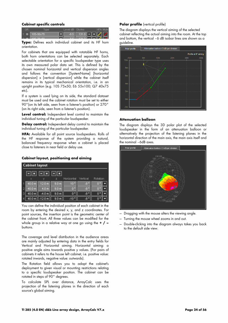
Cabinet specific controls

Type: Defines each individual cabinet and its HF hornorientation.

For cabinets that are equipped with rotatable HF horns,both horn orientations can be selected separately. Eachselectable orientation for a specific loudspeaker type usesits own measured polar data set. This is defined by thechosen nominal horizontal and vertical dispersion anglesand follows the convention [SystemName] [horizontaldispersion] x [vertical dispersion] while the cabinet itselfremains in its typical mechanical orientation, i.e. in anupright position (e.g. 10S 75x50; E6 55x100; Q7 40x75etc).

If a system is used lying on its side, the standard datasetmust be used and the cabinet rotation must be set to either90°(on its left side, seen from a listener's position) or 270°(on its right side, seen from a listener's position).

Level control: Independent level control to maintain theindividual tuning of the particular loudspeaker.

Delay control: Independent delay control to maintain theindividual tuning of the particular loudspeaker.

HFA: Available for all point source loudspeakers. Rolls ofthe HF response of the system providing a natural,balanced frequency response when a cabinet is placedclose to listeners in near field or delay use.

Cabinet layout, positioning and aiming

You can define the individual position of each cabinet in theroom by entering the desired x, y, and z coordinates. Forpoint sources, the insertion point is the geometric center ofthe cabinet front. All three values can be modified for thewhole group in a relative way at one go using the + / –buttons.

The coverage and level distribution in the audience areasare mainly adjusted by entering data in the entry fields forVertical and Horizontal aiming. Horizontal aiming: apositive angle aims towards positive y values. (For pairs ofcabinets it refers to the house left cabinet, i.e. positive value:rotated inwards, negative value: outwards).

The Rotation field allows you to adapt the cabinet'sdeployment to given visual or mounting restrictions relatingto a specific loudspeaker position. The cabinet can berotated in steps of 90° degrees.

To calculate SPL over distance, ArrayCalc uses theprojection of the listening planes in the direction of eachsource's global aiming.

Polar profile (vertical profile)

The diagram displays the vertical aiming of the selectedcabinet reflecting the actual aiming into the room. At the topand bottom, the vertical –6 dB isobar lines are shown as aguideline.

Attenuation balloon

The diagram displays the 3D polar plot of the selectedloudspeaker in the form of an attenuation balloon oralternatively the projection of the listening planes in thehorizontal direction of the main axis, the main axis itself andthe nominal –6dB axes.

— Dragging with the mouse alters the viewing angle.

— Turning the mouse wheel zooms in and out.

— Double-clicking into the diagram always takes you backto the default side view.


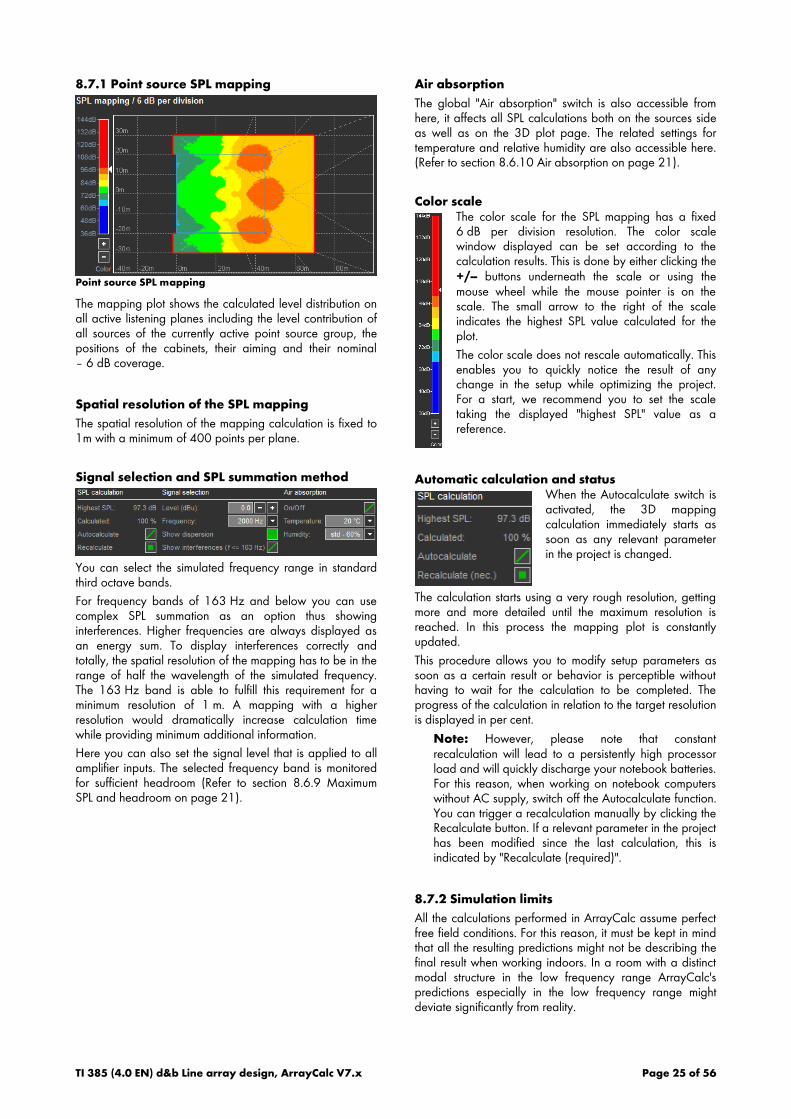
8.7.1 Point source SPL mapping

Point source SPL mapping

The mapping plot shows the calculated level distribution onall active listening planes including the level contribution ofall sources of the currently active point source group, thepositions of the cabinets, their aiming and their nominal– 6 dB coverage.

Spatial resolution of the SPL mapping

The spatial resolution of the mapping calculation is fixed to1m with a minimum of 400 points per plane.

Signal selection and SPL summation method

You can select the simulated frequency range in standardthird octave bands.

For frequency bands of 163 Hz and below you can usecomplex SPL summation as an option thus showinginterferences. Higher frequencies are always displayed asan energy sum. To display interferences correctly andtotally, the spatial resolution of the mapping has to be in therange of half the wavelength of the simulated frequency.The 163 Hz band is able to fulfill this requirement for aminimum resolution of 1 m. A mapping with a higherresolution would dramatically increase calculation timewhile providing minimum additional information.

Here you can also set the signal level that is applied to allamplifier inputs. The selected frequency band is monitoredfor sufficient headroom (Refer to section 8.6.9 MaximumSPL and headroom on page 21).

Air absorption

The global "Air absorption" switch is also accessible fromhere, it affects all SPL calculations both on the sources sideas well as on the 3D plot page. The related settings fortemperature and relative humidity are also accessible here.(Refer to section 8.6.10 Air absorption on page 21).

Color scaleThe color scale for the SPL mapping has a fixed6 dB per division resolution. The color scalewindow displayed can be set according to thecalculation results. This is done by either clicking the+/-- buttons underneath the scale or using themouse wheel while the mouse pointer is on thescale. The small arrow to the right of the scaleindicates the highest SPL value calculated for theplot.

The color scale does not rescale automatically. Thisenables you to quickly notice the result of anychange in the setup while optimizing the project.For a start, we recommend you to set the scaletaking the displayed "highest SPL" value as areference.

Automatic calculation and statusWhen the Autocalculate switch isactivated, the 3D mappingcalculation immediately starts assoon as any relevant parameterin the project is changed.

The calculation starts using a very rough resolution, gettingmore and more detailed until the maximum resolution isreached. In this process the mapping plot is constantlyupdated.

This procedure allows you to modify setup parameters assoon as a certain result or behavior is perceptible withouthaving to wait for the calculation to be completed. Theprogress of the calculation in relation to the target resolutionis displayed in per cent.

Note: However, please note that constantrecalculation will lead to a persistently high processorload and will quickly discharge your notebook batteries.For this reason, when working on notebook computerswithout AC supply, switch off the Autocalculate function.You can trigger a recalculation manually by clicking theRecalculate button. If a relevant parameter in the projecthas been modified since the last calculation, this isindicated by "Recalculate (required)".

8.7.2 Simulation limits

All the calculations performed in ArrayCalc assume perfectfree field conditions. For this reason, it must be kept in mindthat all the resulting predictions might not be describing thefinal result when working indoors. In a room with a distinctmodal structure in the low frequency range ArrayCalc'spredictions especially in the low frequency range mightdeviate significantly from reality.


8.8 SUB arrays

8.8.1 General considerations on stackedsubwoofer placement

The intention of a SUB array is to distribute the availablelow frequency energy as evenly as possible.

ArrayCalc calculates the dispersion and coverage ofhorizontal SUB arrays for different LF bands. It provides thenecessary individual delay settings of the subwoofers toachieve the desired array directivity.

ArrayCalc applies a complex summation (vectorsummation) of all sources of the SUB array for a fixednumber of sample points distributed evenly across thedisplayed area. For all subwoofer types high resolutiondispersion data is used containing both amplitude andphase information.

For SUB arrays as well as for a standard L/R setup,ArrayCalc allows to calculate the overall time alignmentbetween ground stacked subwoofers and a selectablearray in the project to provide a correct system impulseresponse. This procedure is performed on the Alignmentpage, which is described in detail in section 8.9.1 Timealignment of SUB arrays on page 33.

Sources page, SUB array selected

8.8.2 L/R ground stack

A conventional L/R subwoofer configuration provides thebest coupling between the individual subwoofer cabinets,thus providing highest efficiency and best impulse response.However, this only applies to the setup center axis. A lookat the SPL mapping at 50 Hz shows all the well-known sideeffects: The power alley in the center, the cancellationzones to the left and right of the center, repeated powerzones, etc.

50 Hz mapping L/R subwoofer setup

A common approach to change this behavior is to add anadditional center source. A look at the SPL mapping of a L/C/R subwoofer arrangement at 50 Hz shows: The zone inthe center of the audience area is more even, but from thesecond cancellation zone, it isn't any better.

50 Hz mapping L/C/R subwoofer setup


8.8.3 Design criteria

Two sources, which are spaced at a distance of half thewavelength of the frequency they reproduce, cancel eachother out in the direction of their connecting line. Forfrequencies higher than this, the cancellation axis turns moreand more towards the center axis while a second maximumappears and increases in level with rising frequency.

In the L/R example above, where the distance from left toright is 18 m (59 ft) (which is more than 2.5 times thewavelength at 50 Hz), the main lobe is in the center, thereare 2 side lobes with cancellation zones in between andbeyond, and the third side lobe is just about to appearclearly.

Consequently, to have full control over the array behaviorwithin the entire operating bandwidth of the subwoofers,the source spacing must be close enough to fulfill the half-wavelength criteria mentioned above for the highestfrequencies at which the subwoofers operate. In the actualapplication, the criteria can be undermined slightly: Firstly,because a subwoofer cabinet is not a theoretical pointsource, but has a certain extension, so the spacing betweencabinet centers can be slightly wider than exactly half thewavelength; secondly, when directional (cardioid)subwoofers are used, they already have a certain rejectiontowards the sides, so the unwanted side lobes aresuppressed to a certain degree.

8.8.4 Physical placement of cabinets

The first step is to array multiple omnidirectional subwoofers(e.g. Q-SUBs) in a line, close enough to avoid lobing. This isquite common practice. A look at the 50 Hz distribution ofan array of 10 subwoofers, equally spaced along 18 m(59 ft), shows a strong center lobe that drops quickly bymore than 12 dB towards the sides of the audience area.

50 Hz mapping of a straight array of 10 subwoofers

It is also clearly visible that the behavior is identical in thedirection of the audience area as well as in the direction ofthe stage.

Curving the array physically widens the dispersion, thusproviding a more useful coverage.

50 Hz mapping of a physically curved 10-source SUB array

This arrangement has two significant disadvantages. Firstly,it occupies positions hardly available for subwooferplacement in reality; secondly, it creates an energy focus onthe stage center which is very difficult or even impossible tohandle with many open microphones.


8.8.5 Shaping the wavefront using delays

The above examples show that our aim is to achieve theperformance of a curved array towards the audience area,but without the increased stage levels and with a realisticspace requirement.

Transforming the physical arc into a delay pattern achievesthe desired performance while avoiding the space problemand reducing the low frequency peak at the center of thestage by about 6 dB.

50 Hz mapping of 10 delay-arced omnidirectionalsubwoofers

Array of directional (cardioid) subwoofers

Distributed SUB arrays with their dispersion designed with adelayed arc, set up from directional subwoofers (cardioidor hypercardioid) offer exceptional control possibilities ofthe low frequency energy while keeping the on-stage lowfrequency level at a minimum. The following plot uses theidentical delay pattern as the one above but theomnidirectional subwoofers are replaced by cardioid ones.Note the reduction of the on-stage level of 12 to 18 dB.

50 Hz mapping of 10 cardioid delay-arced subwoofers

Furthermore, directional subwoofers allow to manipulate thedispersion pattern by rotating the single cabinets about theirvertical axes. If they are well arranged, this allows for verywide array dispersions while maintaining low on-stagelevels.


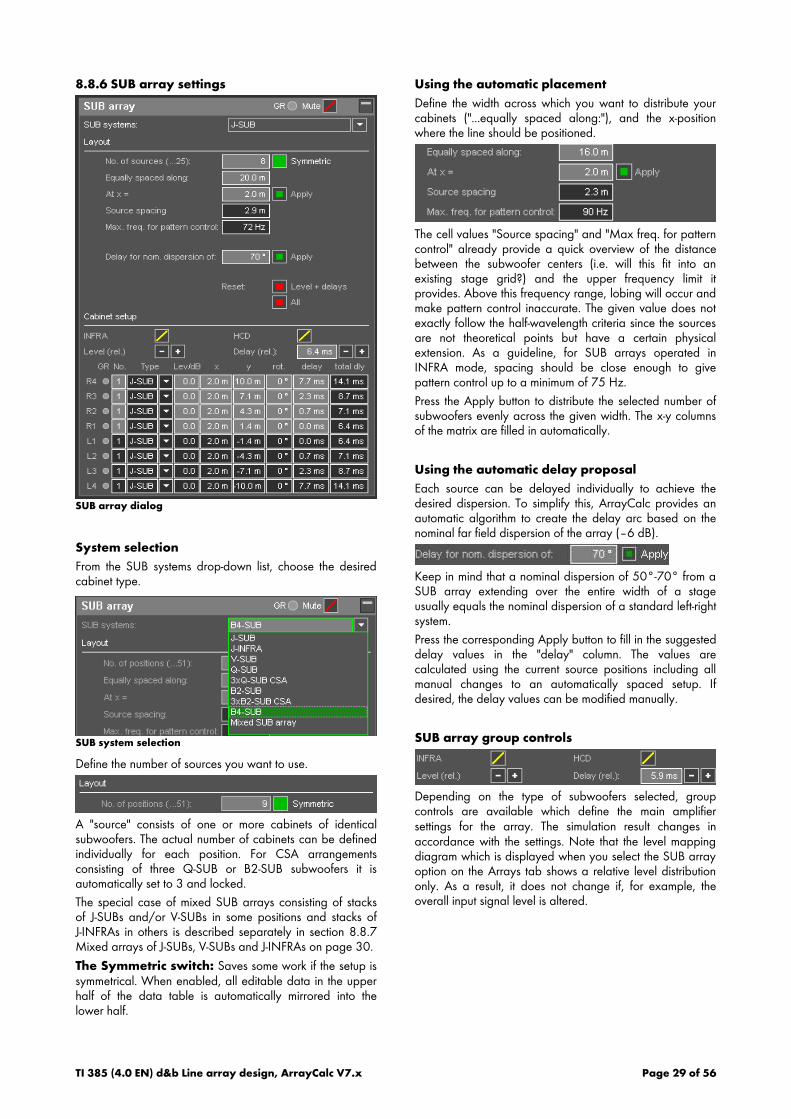
8.8.6 SUB array settings

SUB array dialog

System selection

From the SUB systems drop-down list, choose the desiredcabinet type.

SUB system selection

Define the number of sources you want to use.

A "source" consists of one or more cabinets of identicalsubwoofers. The actual number of cabinets can be definedindividually for each position. For CSA arrangementsconsisting of three Q-SUB or B2-SUB subwoofers it isautomatically set to 3 and locked.

The special case of mixed SUB arrays consisting of stacksof J-SUBs and/or V-SUBs in some positions and stacks ofJ-INFRAs in others is described separately in section 8.8.7Mixed arrays of J-SUBs, V-SUBs and J-INFRAs on page 30.

The Symmetric switch: Saves some work if the setup issymmetrical. When enabled, all editable data in the upperhalf of the data table is automatically mirrored into thelower half.

Using the automatic placement

Define the width across which you want to distribute yourcabinets ("...equally spaced along:"), and the x-positionwhere the line should be positioned.

The cell values "Source spacing" and "Max freq. for patterncontrol" already provide a quick overview of the distancebetween the subwoofer centers (i.e. will this fit into anexisting stage grid?) and the upper frequency limit itprovides. Above this frequency range, lobing will occur andmake pattern control inaccurate. The given value does notexactly follow the half-wavelength criteria since the sourcesare not theoretical points but have a certain physicalextension. As a guideline, for SUB arrays operated inINFRA mode, spacing should be close enough to givepattern control up to a minimum of 75 Hz.

Press the Apply button to distribute the selected number ofsubwoofers evenly across the given width. The x-y columnsof the matrix are filled in automatically.

Using the automatic delay proposal

Each source can be delayed individually to achieve thedesired dispersion. To simplify this, ArrayCalc provides anautomatic algorithm to create the delay arc based on thenominal far field dispersion of the array (–6 dB).

Keep in mind that a nominal dispersion of 50°-70° from aSUB array extending over the entire width of a stageusually equals the nominal dispersion of a standard left-rightsystem.

Press the corresponding Apply button to fill in the suggesteddelay values in the "delay" column. The values arecalculated using the current source positions including allmanual changes to an automatically spaced setup. Ifdesired, the delay values can be modified manually.

SUB array group controls

Depending on the type of subwoofers selected, groupcontrols are available which define the main amplifiersettings for the array. The simulation result changes inaccordance with the settings. Note that the level mappingdiagram which is displayed when you select the SUB arrayoption on the Arrays tab shows a relative level distributiononly. As a result, it does not change if, for example, theoverall input signal level is altered.


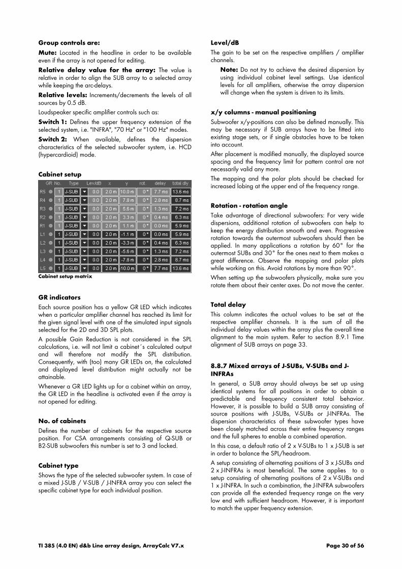
Group controls are:

Mute: Located in the headline in order to be availableeven if the array is not opened for editing.

Relative delay value for the array: The value isrelative in order to align the SUB array to a selected arraywhile keeping the arc-delays.

Relative levels: Increments/decrements the levels of allsources by 0.5 dB.

Loudspeaker specific amplifier controls such as:

Switch 1: Defines the upper frequency extension of theselected system, i.e. "INFRA", "70 Hz" or "100 Hz" modes.

Switch 2: When available, defines the dispersioncharacteristics of the selected subwoofer system, i.e. HCD(hypercardioid) mode.

Cabinet setup

Cabinet setup matrix

GR indicators

Each source position has a yellow GR LED which indicateswhen a particular amplifier channel has reached its limit forthe given signal level with one of the simulated input signalsselected for the 2D and 3D SPL plots.

A possible Gain Reduction is not considered in the SPLcalculations, i.e. will not limit a cabinet´s calculated outputand will therefore not modify the SPL distribution.Consequently, with (too) many GR LEDs on, the calculatedand displayed level distribution might actually not beattainable.

Whenever a GR LED lights up for a cabinet within an array,the GR LED in the headline is activated even if the array isnot opened for editing.

No. of cabinets

Defines the number of cabinets for the respective sourceposition. For CSA arrangements consisting of Q-SUB orB2-SUB subwoofers this number is set to 3 and locked.

Cabinet type

Shows the type of the selected subwoofer system. In case ofa mixed J-SUB / V-SUB / J-INFRA array you can select thespecific cabinet type for each individual position.

Level/dB

The gain to be set on the respective amplifiers / amplifierchannels.

Note: Do not try to achieve the desired dispersion byusing individual cabinet level settings. Use identicallevels for all amplifiers, otherwise the array dispersionwill change when the system is driven to its limits.

x/y columns - manual positioning

Subwoofer x/y-positions can also be defined manually. Thismay be necessary if SUB arrays have to be fitted intoexisting stage sets, or if single obstacles have to be takeninto account.

After placement is modified manually, the displayed sourcespacing and the frequency limit for pattern control are notnecessarily valid any more.

The mapping and the polar plots should be checked forincreased lobing at the upper end of the frequency range.

Rotation - rotation angle

Take advantage of directional subwoofers: For very widedispersions, additional rotation of subwoofers can help tokeep the energy distribution smooth and even. Progressiverotation towards the outermost subwoofers should then beapplied. In many applications a rotation by 60° for theoutermost SUBs and 30° for the ones next to them makes agreat difference. Observe the mapping and polar plotswhile working on this. Avoid rotations by more than 90°.

When setting up the subwoofers physically, make sure yourotate them about their center axes. Do not move the center.

Total delay

This column indicates the actual values to be set at therespective amplifier channels. It is the sum of all theindividual delay values within the array plus the overall timealignment to the main system. Refer to section 8.9.1 Timealignment of SUB arrays on page 33.

8.8.7 Mixed arrays of J-SUBs, V-SUBs and J-INFRAs

In general, a SUB array should always be set up usingidentical systems for all positions in order to obtain apredictable and frequency consistent total behavior.However, it is possible to build a SUB array consisting ofsource positions with J-SUBs, V-SUBs or J-INFRAs. Thedispersion characteristics of these subwoofer types havebeen closely matched across their entire frequency rangesand the full spheres to enable a combined operation.

In this case, a default ratio of 2 x V-SUBs to 1 x J-SUB is setin order to balance the SPL/headroom.

A setup consisting of alternating positions of 3 x J-SUBs and2 x J-INFRAs is most beneficial. The same applies to asetup consisting of alternating positions of 2 x V-SUBs and1 x J-INFRA. In such a combination, the J-INFRA subwooferscan provide all the extended frequency range on the verylow end with sufficient headroom. However, it is importantto match the upper frequency extension.


If you have selected a mixed array of J/V-SUB and J-INFRAsubwoofers in the SUB systems drop-down list, the cabinettypes listed in the Cabinet setup section are displayed in alist box from which you can select the system for eachposition.

The bandwidth selection switches (Switch 1) of the twosystems work in reverse, i.e the J-SUB has an "INFRA" (theV-SUB a 100 Hz) switch lowering the upper frequencyextension when "on", while the J-INFRA has a "70 Hz"switch rising the upper frequency extension when "on".Consequently, they have to be combined and are mutuallyexclusive. When you activate one, the other one isdisabled. Their proper use is controlled by the "hip/hop"selector.

8.8.8 Dispersion displays

The following displays help to evaluate the performance ofthe array.

Mapping diagram

Select the simulation frequency.

Consider and compare all relevant frequencies within thesystem´s operating bandwidth. Each colored isobarrepresents a drop in level by 6 dB. Place the mouse ontothe drop-down list and use the wheel to quickly changebetween the frequencies.

Mapping diagram with color scale

Color scale

The color scale for the SPL mapping has a fixed 6 dB perdivision resolution. The color scale window displayed canbe set according to the calculation results. This is done byeither clicking the +/-- buttons underneath the scale orusing the mouse wheel while the mouse pointer is on thescale. The small arrow to the right of the scale indicates thehighest SPL value calculated for the plot.

The color scale does not rescale automatically. This enablesyou to quickly notice the result of any change in the setupwhile optimizing the project.

Polar diagram

Polar diagrams visualize the far field behavior of the array,i.e. the dispersion pattern at a distance which is much largerthan the array dimensions.

Although this distance might often extend beyond the actualaudience area, the polar diagram provides helpfulinformation about the consistency of the dispersion patternsfor different frequency bands displayed in a single plot.

Third-octave frequency bands between 32 Hz and 100 Hzcan be selected, as well as the octave average at 40 Hzand 80 Hz.

Polar diagram

Use the Alignment page to calculate the correct timealignment between the SUB array and a selectable flownarray with the help of a phase matching procedure (refer tosection 8.9.1 Time alignment of SUB arrays on page 33).


8.9 Alignment page

For a complex system consisting of multiple sources it isessential to time align the different parts in a useful way.ArrayCalc provides a dedicated Alignment page to helpyou find a useful alignment strategy and finally deducestarting values.

Alignment

The left side of the page contains a fully operable copy ofthe project, room and source settings of the project.

Selecting the test point for array alignment

Within a copy of the Top view diagram, a test point can bechosen either by clicking in the diagram and/or by movingaround using the arrow buttons next to its x-/y-coordinatesor by directly entering numerical values.

The z-coordinate is calculated based on the x/y positionand on the presence of a listening plane at this position.When you move the point, the algorithm keeps it on thesame plane as long as possible. If the end of a plane isreached, it jumps onto the next plane in the direction ofmoving. The Current plane field shows the name of theplane on which the test point is currently located.

Arrival times diagram

Arrival times diagram including point sources

The arrival times diagram shows the first arrival of acousticenergy reaching the test point in milliseconds for all arraysor individual sources in the project provided they areunmuted. Underneath the diagram you can define muteand delay settings for each array. In case of an array, bothfunctions are operable copies of the same functions in thearray settings dialog of each array.

The Delay settings can be defined by entering data directlyinto the relevant field of each array or using the +/--buttons. Holding down the CTRL key (Apple key forMacintosh) while clicking the +/-- buttons switches from fineto coarse increments.

In case of a point source group, the Mute switch here mutesor unmutes the entire group. If you want to mute/unmutethe individual sources of the group, you have to go to theappropriate point source settings dialog. The delay buttonsfor a point source group increment/decrement the delayvalues for all sources of the group while keeping theirsettings relative to each other. As a result, a numeric datainput field is not available here.

In the above example, the test point is located at a positionto align the "Outfill" array to the "Main Array" array. Thefirst arrival time from the left side of the paired "Outfill"array is around 110 ms, while the arrival time of the leftside of the paired "Main L/R" array is around 114 ms. Thatmeans, approximately 4 ms of delay have to be added tothe "Outfill" array to set a correct time arrival for this testpoint position.

In this example, the left sides (L) of the paired arrays weretaken as a basis because they are closer to the test pointthan the right sides. The peaks at 148ms and 157 msrepresent the arrival times from the right sides of the pairedarrays. Note their relatively low levels and thereforenegligible influence at the selected position. These peakscan be switched off by simply muting the right sides (R) ofthe paired arrays.

The alignment for point sources is performed in a similarway. Place the test point at a suitable position within thetarget area of each point source and set the delayaccordingly. In case of distributed point sources, it may benecessary to perform this procedure for each individualsource.


8.9.1 Time alignment of SUB arrays

It is vital to carry out a correct time alignment of groundstacked or arrayed subwoofers to the main system.ArrayCalc accurately calculates the settings necessary foran optimum alignment at a user-defined distance from thesystem, thus replacing a measurement system.

Note: Before evaluating the necessary time alignment,make sure all mechanical and acoustic parameters aswell as the arc-shaping delay times of the SUB arrayare set correctly and correspond to the actual setup atthe venue. Verify all actual distances, positions and trimheights. Wrong parameters will deliver an incorrectalignment. If in doubt, use an acoustic measurementsystem to set the delays (refer to section 9.5 Timealignment on page 42).

Make sure to use the final delay setting for the selectedsource to which the subwoofers are to be aligned. If thesource delays are modified later, the subwoofer alignmenthas to be re-checked.

Selecting the source for alignment

Select one of the sources in the project for phase alignmentwith the SUB array. Make sure to select a source with atarget dispersion that is reasonably similar to the SUB array.

Selecting the test point

You can select the distance (x value) at which the phaseresponses of the SUB array and the source are compared.This test point is always located at the y-position of the leftsource selected. This provides a good alignment result for awide area in the infield of an audience area, including theFoH position. Choose an x-position at a sufficient distancefrom the sources. Usually a typical FoH position is a goodchoice.

Calculating the phase response

The phase responses of both the selected source and theSUB array at the test point are calculated using a complexsum of all contributing sources including their angle-dependent phase and level response, and delay settings.To obtain a useful phase plot, the distance of the closestsource to the test point is compensated for in the diagram.

Set both delay values to minimum (0.3 ms) and checkwhich system sound arrives earlier (selected source orSUBs).

It is the one with fewer "turns" in the phase response, sincea steeper phase curve means more delay.

Phase response - not aligned

In the above example it is the white trace representing thesummed response of the SUB array, indicating that the SUBarray needs additional delay for phase matching.

Gradually increase the delay of the earlier signal until thetwo phase traces match each other within the relevantfrequency range ~55 Hz and ~120 Hz (dark area) aswell as possible.

Phase response - correctly aligned

Aligning a L/R subwoofer setup

The delay alignment tool can also be used to align L/Rground stacked subwoofers to any other source. Set thenumber of subwoofer sources to 1. Now only the centersource is active. Enter the x and y coordinates of the leftground stack and proceed as before.


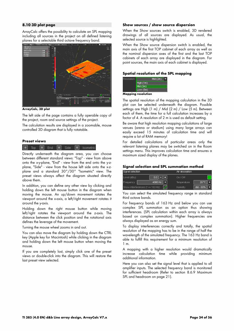
8.10 3D plot page

ArrayCalc offers the possibility to calculate an SPL mappingincluding all sources in the project on all defined listeningplanes for a selectable third octave frequency band.

ArrayCalc, 3D plot

The left side of the page contains a fully operable copy ofthe project, room and source settings of the project.

The calculation results are displayed in a zoomable, mousecontrolled 3D diagram that is fully rotatable.

Preset views

Directly underneath the diagram area, you can choosebetween different standard views: "Top" - view from aboveonto the x-y-plane, "End" - view from the end onto the y-z-plane, "Side" - view from the house left side onto the x-z-plane and a standard 30°/30° "Isometric" view. Thepreset views always affect the diagram situated directlyabove them.

In addition, you can define any other view by clicking andholding down the left mouse button in the diagram whenmoving the mouse. An up/down movement rotates theviewport around the x-axis, a left/right movement rotates itaround the y-axis.

Holding down the right mouse button while movingleft/right rotates the viewport around the z-axis. Thedistance between the click position and the rotational axisdefines the leverage of the movement.

Turning the mouse wheel zooms in and out.

You can also move the diagram by holding down the CTRLkey (Apple key for Macintosh) while clicking in the diagramand holding down the left mouse button when moving themouse.

If you are completely lost, simply click one of the presetviews or double-click into the diagram. This will restore thelast preset view selected.

Show sources / show source dispersion

When the Show sources switch is enabled, 3D rendereddrawings of all sources are displayed. As usual, theselected source is highlighted.

When the Show source dispersion switch is enabled, themain axis of the first TOP cabinet of each array as well asthe nominal dispersion axes of the first and the last TOPcabinets of each array are displayed in the diagram. Forpoint sources, the main axis of each cabinet is displayed.

Spatial resolution of the SPL mapping

Mapping resolution

The spatial resolution of the mapping calculation in the 3Dplot can be selected underneath the diagram. Possiblesettings are High (1 m) / Mid (2 m) / Low (5 m). Betweeneach of them, the time for a full calculation increases by afactor of 4. A resolution of 2 m is used as default setting.

Be aware that high resolution mapping calculations of largevenues (arena or stadium) using many large arrays caneasily exceed 15 minutes of calculation time and willrequire a lot of RAM memory!

For detailed calculations of particular areas only therelevant listening planes may be switched on in the Roomsettings menu. This improves calculation time and ensures amaximum sized display of the planes.

Signal selection and SPL summation method

You can select the simulated frequency range in standardthird octave bands.

For frequency bands of 163 Hz and below you can usecomplex SPL summation as an option thus showinginterferences. (SPL calculation within each array is alwaysbased on complex summation). Higher frequencies arealways displayed as an energy sum.

To display interferences correctly and totally, the spatialresolution of the mapping has to be in the range of half thewavelength of the simulated frequency. The 163 Hz band isable to fulfill this requirement for a minimum resolution of1 m.

A mapping with a higher resolution would dramaticallyincrease calculation time while providing minimumadditional information.

Here you can also set the signal level that is applied to allamplifier inputs. The selected frequency band is monitoredfor sufficient headroom (Refer to section 8.6.9 MaximumSPL and headroom on page 21).


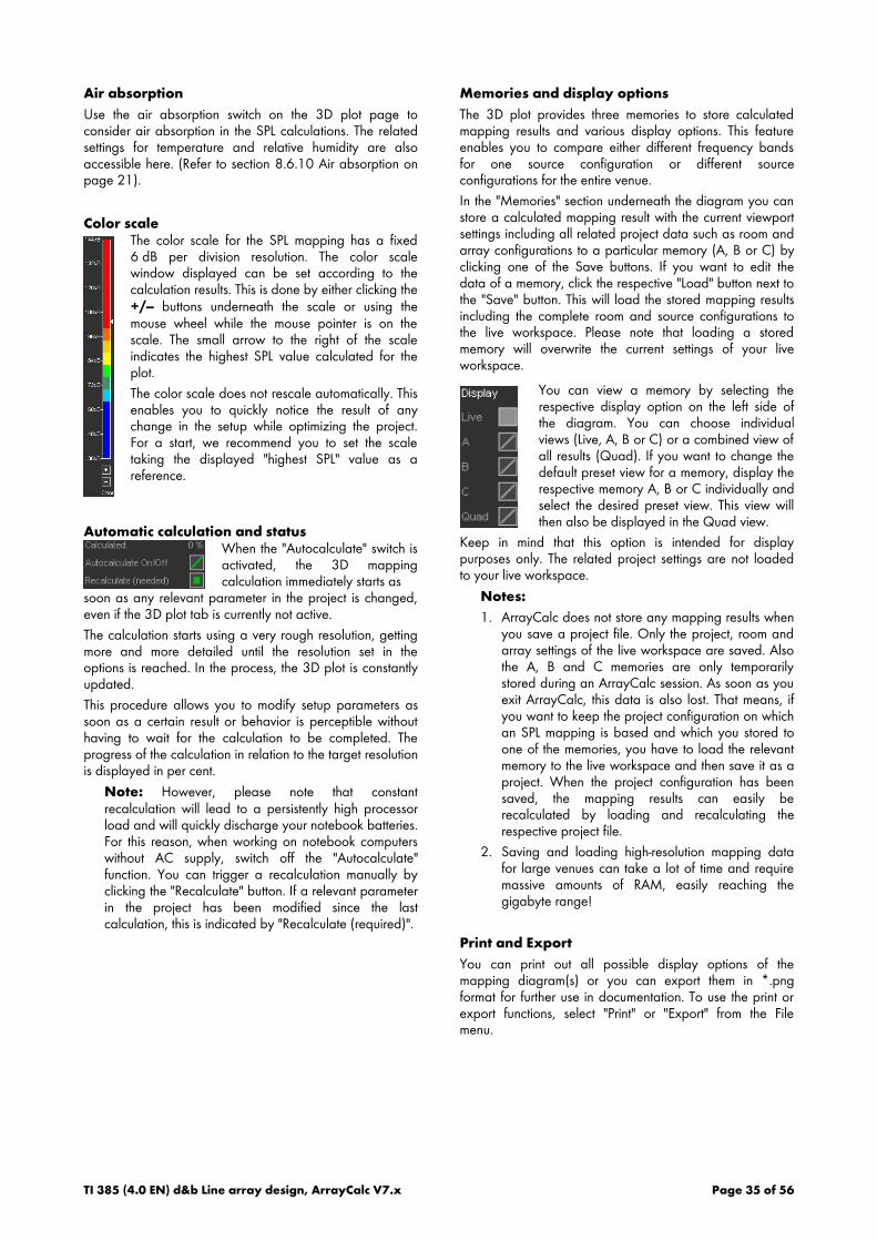
Air absorption

Use the air absorption switch on the 3D plot page toconsider air absorption in the SPL calculations. The relatedsettings for temperature and relative humidity are alsoaccessible here. (Refer to section 8.6.10 Air absorption onpage 21).

Color scaleThe color scale for the SPL mapping has a fixed6 dB per division resolution. The color scalewindow displayed can be set according to thecalculation results. This is done by either clicking the+/-- buttons underneath the scale or using themouse wheel while the mouse pointer is on thescale. The small arrow to the right of the scaleindicates the highest SPL value calculated for theplot.

The color scale does not rescale automatically. Thisenables you to quickly notice the result of anychange in the setup while optimizing the project.For a start, we recommend you to set the scaletaking the displayed "highest SPL" value as areference.

Automatic calculation and statusWhen the "Autocalculate" switch isactivated, the 3D mappingcalculation immediately starts as

soon as any relevant parameter in the project is changed,even if the 3D plot tab is currently not active.

The calculation starts using a very rough resolution, gettingmore and more detailed until the resolution set in theoptions is reached. In the process, the 3D plot is constantlyupdated.

This procedure allows you to modify setup parameters assoon as a certain result or behavior is perceptible withouthaving to wait for the calculation to be completed. Theprogress of the calculation in relation to the target resolutionis displayed in per cent.

Note: However, please note that constantrecalculation will lead to a persistently high processorload and will quickly discharge your notebook batteries.For this reason, when working on notebook computerswithout AC supply, switch off the "Autocalculate"function. You can trigger a recalculation manually byclicking the "Recalculate" button. If a relevant parameterin the project has been modified since the lastcalculation, this is indicated by "Recalculate (required)".

Memories and display options

The 3D plot provides three memories to store calculatedmapping results and various display options. This featureenables you to compare either different frequency bandsfor one source configuration or different sourceconfigurations for the entire venue.

In the "Memories" section underneath the diagram you canstore a calculated mapping result with the current viewportsettings including all related project data such as room andarray configurations to a particular memory (A, B or C) byclicking one of the Save buttons. If you want to edit thedata of a memory, click the respective "Load" button next tothe "Save" button. This will load the stored mapping resultsincluding the complete room and source configurations tothe live workspace. Please note that loading a storedmemory will overwrite the current settings of your liveworkspace.

You can view a memory by selecting therespective display option on the left side ofthe diagram. You can choose individualviews (Live, A, B or C) or a combined view ofall results (Quad). If you want to change thedefault preset view for a memory, display therespective memory A, B or C individually andselect the desired preset view. This view willthen also be displayed in the Quad view.

Keep in mind that this option is intended for displaypurposes only. The related project settings are not loadedto your live workspace.

Notes:

1. ArrayCalc does not store any mapping results whenyou save a project file. Only the project, room andarray settings of the live workspace are saved. Alsothe A, B and C memories are only temporarilystored during an ArrayCalc session. As soon as youexit ArrayCalc, this data is also lost. That means, ifyou want to keep the project configuration on whichan SPL mapping is based and which you stored toone of the memories, you have to load the relevantmemory to the live workspace and then save it as aproject. When the project configuration has beensaved, the mapping results can easily berecalculated by loading and recalculating therespective project file.

2. Saving and loading high-resolution mapping datafor large venues can take a lot of time and requiremassive amounts of RAM, easily reaching thegigabyte range!

Print and Export

You can print out all possible display options of themapping diagram(s) or you can export them in *.pngformat for further use in documentation. To use the print orexport functions, select "Print" or ''Export" from the Filemenu.


8.11 R1 Export page

The ArrayCalc export function for R1 project files provides afast and convenient way to transfer the whole system setupcreated in ArrayCalc to an R1 remote control user interface.In addition, the R1 Export function also includes an optionfor printing out a patch plan.

At the click of a button ArrayCalc creates an R1 project file(.rop) containing the amplifiers (devices) and all groupsand control elements to operate the system simulated inArrayCalc. The structure of this project file corresponds tothe design of an R1 project file as described in TI 391"Effective use of R1".

8.11.1 Export R1 files

In addition to the R1 project file, an R1 Control settings filecontaining all settings for the devices and group controls iscreated. You can load this file in R1 by clicking theappropriate button on the Overview page of the exportedR1 project.

To maintain integrity between an R1 project file and thecontrol settings, the two files can only be exported together.

After having changed controller settings (e.g. levels, delaysor CUT/HFC settings), you can export a new set of filesand load the control settings in R1 without having toreplace the project file.

Note: Please note, however, that if your changes affectthe actual setups of the devices (e.g. IDs or Arc/Linesetups), you have to create a new project file and openit in R1.

Standard procedure

To make effective use of the R1 Export feature, proceed asfollows:

1. Use the Link cabinets function at the top of the R1Export page. If necessary, adapt the patch of individual devicesmanually. A detailed description is given in section8.11.3 Patch dialog on page 36.

2. Use the Configure amplifiers function at the top of theR1 Export page.If necessary, adapt the configuration of individualdevices manually. A detailed description is given insection 8.11.4 Cabinets section on page 37.

3. Click the Export R1 files button and save the R1 projectfile and the Control settings file.

4. Open the R1 project file in R1.

5. Load the Control settings using the appropriate buttonon the Overview page of the exported R1 project.

Patch plan printout

ArrayCalc provides you with a detailed patch plan printoutincluding the chosen input type and source. On the R1Export page select 'Print' from the File menu or press Ctrl+P(CMD+P for Mac OS X systems).

8.11.2 Patches

The R1 Export page provides a patch dialog for each arrayin the project to allow individual assignment (patch) of thecabinets to the respective amplifier channels. Additionallythe dialog allows you to configure several settings forremote control in R1.

Link cabinets function

Clicking the Link cabinets button at the top of the R1 Exportpage links the recommended number of cabinets to oneamplifier channel. This function applies to all arrays in oneproject (including the additional devices), whether they areopen or not.

Note: Please note that only adjacent cabinets withidentical level and switch settings are linked. ArrayCalcdoes not share amplifier channels between differentarrays. For this reason, unused amplifier channels willnot be used on other arrays but will be listed in theUnused channels section at the bottom of each array.

Configure amplifiers function

Clicking the Configure amplifiers button at the top of the R1Export page creates a default order of device IDs andchannel A/B settings for the entire project. Amplifier IDsstart at 0.01 for the top left cabinet of the first array in thelist. You can also specify a Start ID manually as describedin section Start ID on page 33.

When you click the Configure all amplifiers button,ArrayCalc displays a dialog asking you whether the StartIDs you specified should be taken into account. If you select"Use Start IDs", the system will start counting from thespecified IDs.

8.11.3 Patch dialog

ArrayCalc provides separate patch dialogs for line arrays,point source groups and the SUB array. Such a patchdialog displays the name of the related source and is splitinto a header and a cabinets section.

Device name prefix

The device name of each amplifier is automaticallygenerated automatically by the system and consists of thefirst 10 characters of the name of the respective source plusthe CAN-ID of the amplifier. The device name cannot beedited itself but it is possible to change its prefix bychanging the name of the respective source in the sourcesettings dialog of the Sources page.


CAN channel (CAN ch.)

This option sets all devices of a patch dialog to the same R1CAN interface channel.

Note: Please note that using this option will overwriteall CAN interface channels you manually set forindividual devices in this dialog. The default setting isCAN interface channel A. For further information onCAN channels, please refer to the R1 manual.

Total number of D12/D6 (Total D12/D6)

ArrayCalc displays the total number of D12/D6 amplifiersused in the currently opened patch dialog. To obtain thetotal number of all amplifiers in a project, please refer to theParts list page.

Note: Please note that the total number of all amplifierson the Parts list page depends on your settings on theR1 export page.

8.11.4 Cabinets section

Link cabinets

Clicking the Link cabinets button at the top of the Cabinetssection of a particular array links the recommended numberof cabinets to one amplifier channel for the whole of thisarray. Alternatively, clicking the link button that is locatednext to an individual cabinet assigns this cabinet to theamplifier channel above and no entry will be created for itin the R1 device list.

Channel name

By default, the system suggests a channel namedetermined by the name of the source of which therespective cabinet is a part and the specific position of thecabinet within the array or the group of point sources. Thisname can be edited.

Device

The default device is the D12 amplifier. You can select theD6 amplifier for the loudspeakers that are supported by theD6.

Output mode

For single channel loudspeakers the D12 output can be seteither to Dual channel or to Mix TOP/SUB wiring.

Channel ( )

Select amplifier channel A or B of the device.

CAN channel ( )

Select the R1 CAN interface channel (i.e. the actualphysical interface) to which the device will be connected.The default setting is CAN interface channel A.

CAN-ID ( )

Set the CAN-ID of the device. When editing an ID, makesure the ID is unique. For passive cabinets, set a D12amplifier to Dual Channel or Mix TOP/SUB mode. For2-way active systems, the D12 amplifier will be configuredautomatically. For D6 amplifiers, each ID may be used fortwo device entries. One with Channel A and one withChannel B selected.

If only a single channel of an amplifier is assigned, thesecond channel will be set to LINEAR mode and added tothe Unused channels section at the bottom of each array.

Note: When you press CTRL+ENTER (CMD+ENTERfor Mac OS X systems) while the cursor is placed on anID field, the system automatically moves the cursor tothe next ID field in the row below and increments thisparticular ID based on the ID specified in the fieldabove.

8.11.5 Additional devices for R1 export

Here you can add amplifiers for d&b loudspeakers that arenot part of the particular ArrayCalc setup. Define thenumber of remote groups required and then add devices toeach group. The name of a group may be edited byclicking in the appropriate edit field.

Note: Please note that changing the name of a groupwill reset all channel names to a default value based onthe given new name of the group.


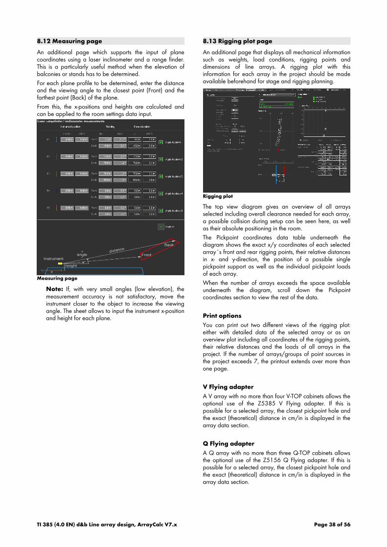
8.12 Measuring page

An additional page which supports the input of planecoordinates using a laser inclinometer and a range finder.This is a particularly useful method when the elevation ofbalconies or stands has to be determined.

For each plane profile to be determined, enter the distanceand the viewing angle to the closest point (Front) and thefarthest point (Back) of the plane.

From this, the x-positions and heights are calculated andcan be applied to the room settings data input.

Measuring page

Note: If, with very small angles (low elevation), themeasurement accuracy is not satisfactory, move theinstrument closer to the object to increase the viewingangle. The sheet allows to input the instrument x-positionand height for each plane.

8.13 Rigging plot page

An additional page that displays all mechanical informationsuch as weights, load conditions, rigging points anddimensions of line arrays. A rigging plot with thisinformation for each array in the project should be madeavailable beforehand for stage and rigging planning.

Rigging plot

The top view diagram gives an overview of all arraysselected including overall clearance needed for each array,a possible collision during setup can be seen here, as wellas their absolute positioning in the room.

The Pickpoint coordinates data table underneath thediagram shows the exact x/y coordinates of each selectedarray´s front and rear rigging points, their relative distancesin x- and y-direction, the position of a possible singlepickpoint support as well as the individual pickpoint loadsof each array.

When the number of arrays exceeds the space availableunderneath the diagram, scroll down the Pickpointcoordinates section to view the rest of the data.

Print options

You can print out two different views of the rigging plot:either with detailed data of the selected array or as anoverview plot including all coordinates of the rigging points,their relative distances and the loads of all arrays in theproject. If the number of arrays/groups of point sources inthe project exceeds 7, the printout extends over more thanone page.

V Flying adapter

A V array with no more than four V-TOP cabinets allows theoptional use of the Z5385 V Flying adapter. If this ispossible for a selected array, the closest pickpoint hole andthe exact (theoretical) distance in cm/in is displayed in thearray data section.

Q Flying adapter

A Q array with no more than three Q-TOP cabinets allowsthe optional use of the Z5156 Q Flying adapter. If this ispossible for a selected array, the closest pickpoint hole andthe exact (theoretical) distance in cm/in is displayed in thearray data section.


8.14 Parts list page

ArrayCalc generates a parts list including all cabinets andrigging components that are required for the specifiedsingle or symmetrical arrays defined in the project. Alsoincluded are the designed SUB array and the cabinets usedfor the groups of point sources. The number of amplifiers isavailable once you have assigned the cabinets to theamplifier channels on the R1 export page.

8.15 Ground stacked setups

WARNING!

Potential risk of personal injury and/ordamage to materials.

Ground stacked arrays must be secured to avoid eitherpossible movement or tipping over.

When a stacked configuration is selected, the array designwill be reversed. Subwoofers will be placed as lowestcabinets. A maximum of 8 cabinets can be selected.

As the Flying frame has to be mounted horizontally, theaiming of the cabinets has to be performed with the help ofsplay angles only, starting with the lowest J/V/Q/T cabinet.There is no Auto splay algorithm available. The height ofthe system is defined by the stage height and the number ofsubwoofers.

Splay setting of the lowest cabinet

J and V-Series arrays are always mounted on theirappropriate Flying frames. The angle options for the lowestcabinet are –3°/0°/+3° for J-Series and –7°/–3.5°/0°/+3.5°/+7° for V-Series and are set in the"Splay to frame/SUB" cell.

Array Calc assumes the use of a standard flying framebetween SUBs and TOPs. If you use other accessories (e.g.Z5386 V Stack adapter), please consider the actualnumber of splay angles available. In this case, thedifference in height must be compensated by modifying the"stage/riser height" accordingly.

With Q1 and T10 arrays the splay value below cabinetno.1 represents the setting according to the scale on thesplay link / cabinet.

When Q Tops are stacked on the Q Flying frame, a valueof 8° results in the cabinet aiming horizontally ("0 toframe"). However, when stacked on a Q-SUB cabinet theactual splay angle between these cabinets has an offset of6°. The setup is best adjusted while watching the absoluteangles of the Q1 cabinets.

When T10 arrays are stacked on a T-Series Flying frame,the splay angle of the lowest cabinet can only be set to –2° or 0°.

When T10 arrays are stacked on a T-SUB cabinet, thesplay angle of the lowest cabinet can be set to –2°, –1°,0°, +1°, +2°, +3°, +4° or +6°.

When T10 arrays are stacked on a T-Series base plate, thesplay angle of the lowest cabinet can range from –8° to+5° (1° increments).

With ground stacked systems the low/mid SPL curvegenerally shows an increase at the very front whenapproaching the stack. Creating a similar curve for thehigh/mid frequencies is not advised as to achieve this thecabinets would have to be placed at the level of thelisteners' ears. This would create dangerous sound pressurelevels at the front, and would not reach the audience at therear.


9. System tuning

The most convenient way to finalize system tuning is to usethe d&b Remote network with the R1 software.

9.1 Arc and Line configurations

For J-, V-, Q- and T-Series loudspeakers the d&b amplifiersprovide two different configurations each and they are setdepending on the mechanical design of the array. The Arc(Q1: standard) configuration is applied when the speakersare used in curved array sections while the Lineconfigurations are used for groups of four or moreloudspeakers when coupled to form a long throw arraysection.

Compared to the Arc (Q1: standard) configuration the Linesetting uses different CPL attenuation functions reducing theupper midrange to compensate for the extended near fieldeffect of the straight array section. With more than twoconsecutive splay settings of 0° or 1° (V, Q1 and T10: 0°,1° or 2°; 10AL(-D): 0°, 1°, 2° or 4°), the Line settingshould be used for the respective cabinets. All the othercabinets should be operated using the Arc (Q1: standard)configuration.

The transition from Line to Arc/standard configuration withinthe array is made according to the splay progression butcertain deviations may be permitted due to the groupedwiring of the cabinets.

You can select the configuration for each individual cabinetin the array settings dialog.

9.2 CUT circuit

Set to CUT, the low frequency level is reduced. The sourceis now configured for use with the system´s dedicatedsubwoofers. The CUT circuit must be set consistently within asource.

You can activate the CUT function using the CUT groupcontrol in the array / point source settings dialog.

9.3 CPL circuit

The CPL (Coupling) circuit compensates for coupling effectsbetween the cabinets by reducing the low and midfrequency level.

You can activate the CPL function using the CPL groupcontrol in the array / point source settings dialog.

J and V-Series

The CPL function should be applied when J or V-TOPcabinets are used in arrays of six (J) or four (V) or morecabinets. As coupling effects change with the length andcurvature of the array, the CPL function differs between Arcand Line setup. Its design enables (and requires) a commonsetting of dB attenuation values between 0 and –9 dB tobe applied to the entire array. CPL begins gradually below2 kHz, with the maximum attenuation below 100 Hz. Athigher attenuation values the corner frequency of the filtershifts towards lower values.

The principal function of the CPL circuit for J-Series cabinetsis shown in the diagram below. Please note that all cabinetswithin a column must be operated at the same CPL setting.

Frequency response correction of the J-Series CPL circuit

Q, T and xA-Series

The Q, T and xA-Series CPL circuits work in a similar way,however the filter corner frequency shifts differentlyaccording to the attenuation to comply with the differentsystem dimensions and curving possibilities. CPL can be setbetween +5 and –9 dB.

Positive CPL values (not supported by ArrayCalc) produce alow frequency boost. This is useful when small arrayswithout additional subwoofers are used for full-rangecoverage. Positive CPL will reduce system headroom.

Frequency response correction of the Q-Series CPL circuit

CPL for point sources

For point sources, CPL compensates for coupling effectsresulting from cabinets mounted close to acousticboundaries, such as walls or rigid ceilings.


9.4 Air absorption and HFC circuit

In addition to the overall loss of sound pressure withincreasing distance, a certain amount of the acousticenergy is absorbed by air. This effect follows a quitecomplex function of mainly frequency, humidity andtemperature.

When the Air Absorption switch is activated, ArrayCalccalculates this effect for selectable temperature andhumidity values. To define the temperature units, clickExtras-Options and choose between degrees Celsius andFahrenheit under Units. The relative humidity can bespecified in 4 steps: "dry-20 %", "low-40 %", "std-60 %" and"high-80 %".

Note that in reality there is not much point in specifyinghumidity values in more detail based on readings taken atone position within an audience area. In almost all cases,this only pretends a high accuracy since these conditionsstrongly vary with height above an audience and that´swhere the sound has to pass through.

When air absorption calculation is selected, you can set theHFC (high frequency compensation) switches and theirsettings will be taken into account in the frequency responseand headroom simulation of the respective cabinets. Whenyou switch off the air absorption calculation, the settings forthe cabinets will be kept and the HFC drop-down lists willbe disabled. In this case, the HFC settings will not be takeninto account. That means, by switching the air absorptioncalculation on or off, you can verify a useful compensationfor the individual amplifier channels when observing thechanges in the high frequency level calculations.

When wiring the cabinets in a column keep in mind that allcabinets linked to one amplifier will be operated at thesame amplifier settings.

The HFC circuits of the J, T and xA-Series configurationshave two settings (HF1, HF2) for the different zones that thecabinets have to cover. The settings should be usedselectively depending on the particular requirements.

Series HFC1 HFC2

J 40 m 80 m

V 30 m 60 m

Q 30 m --

T 25 m 50 m

xA 25 m 50 m

Overview of HFC distance compensation

At lower humidity values absorption by air increasestherefore the distances at which the respective HFC settingsprovide a correct equalization will be shorter.

The HFC2 compensation in the J8/J12, V8/V12, T10 and10AL(-D) Line setups include a bandwidth limitation toapprox. 10 kHz to keep the necessary boost withinmeaningful limits not wasting the system's headroom.

Example of frequency response correction of the HFC circuits


9.5 Time alignment

Within a line array column it is absolutely essential tomaintain perfect time alignment, otherwise the wholeprinciple of creating a coherent wavefront will fail.Therefore, all amplifiers used to drive one column must befed from the same input signal. Should a delay for thecomplete line array be necessary, the delay function in theamplifier channels can be used. The setting must beidentical for all amplifier channels used in the column.

9.5.1 Subwoofers

A correct time alignment of subwoofers to the main linearray is very important. If the required delay settings cannotbe calculated using ArrayCalc (unknown geometry of thesetup, unknown latency of devices in the signal chain), anacoustic measurement system should be used.

The signal arrival at the FoH position can be used as areference for time alignment.

In the following example the subwoofer amplifiers have tobe set to a delay time of Dt, equivalent to the physical offsetDx divided by the speed of sound (343 m/s or 1126 ft/s).

t= x

vsound

Time alignment of ground stacked cabinets

Note: An automatic time alignment using impulseresponses - sometimes called "delay finder" – cannotprovide correct results when systems cover differentfrequency bands, as this is the case with line arraycabinets and subwoofers.

Therefore use the response of the flown array and a full-range speaker placed on top of the subwoofer (e.g.nearfill) to determine the delay setting.

9.5.2 Nearfills

If nearfill loudspeakers are placed on top of subwoofercabinets, the respective amplifier channels have to be set tothe same delay value as the subwoofer.

When applying SUB arrays with extensive delay settings toform the wavefront, equal delay settings of nearfill speakersplaced on top of the subwoofers may not allow for correctsource imaging in some positions. In this case, the correcttiming of the nearfill speaker is of greater importance and apossible local phase mismatch to the subwoofer isacceptable.

9.5.3 Horizontal array

If multiple J/V/Q/T-Series columns or any combination ofthem are used per side, the arrays should be time-alignedat a meaningful position around the direction where bothproduce equal level. Use ArrayCalc's Alignment page toperform the alignment (refer to section 8.9 Alignment pageon page 32).

Should the procedure result in additional delay for thearray selected for the subwoofer alignment, make sure thisis compensated for in the delay settings for the SUB array.To measure the delay setting between subwoofers andmain column on site turn off the outfill column.

Time alignment of a horizontal array

9.6 Equalization

If additional equalization of the system is required, use thed&b amplifier's 4-band fully parametric equalizer. It isimportant when applying the equalization that all channelsare set identically within one column. Using the d&b Remotenetwork and the R1 remote software the amplifier channelsand their equalizers can be operated in user-definedfunctional groups, such as array, subwoofers, or outfill.Please refer to TI 391 "Effective use of R1" which isavailable for download from the d&b audiotechnik websiteat www.dbaudio.com.

Using the amplifier's parametric equalizer for the system EQprovides the sound engineer with a flat FoH EQ for hispersonal sound design.

10. ArrayCalc setup examples

The following plots show a selection of J, V, Q, T andxS/xA-Series array setups for different array sizes andvenues.

All these and additional project files can be accessed forfurther evaluation and modification. To open an exampleproject, select 'Open example project' from the File menu.


10.1 T-Series setup examples

T-Series setup example 1, Arrays: 3 x T10 flown or on T cluster bracket, 2 x B4-SUB

T-Series setup example 3, Arrays: 8 x T10 flown, flat field, 8 x B4 SUB array

TI 385 (4.0 EN), d&b Line array design, ArrayCalc V7.x of 56

T-Series setup example 5, 3D plot: 12 x T10 flown, Arena type venue, 4 xT10 Delay,3 x T10 Outfill, 8 x B4-SUB array


10.2 Q-Series setup examples

Q-Series setup example 3, Arrays: 6 x Q1, 1xQ7 Theater with balcony, 8 x B4-SUB array

Q-Series setup example 3, SUB array: 6 x Q1, 1 x Q7 Theater with balcony, 8 x B4-SUB array


Q-Series setup example 5, Alignment: 15 x Q1, Arena, 6 x Q1 Outfill, 1 x Q7 Center, 8 x J-SUB SUB array


10.3 V-Series setup examples

V-Series setup example 3, Arrays: 6 x V8, 2xV12 Theater with balcony, 8 x V-SUB array

V-Series setup example 3, SUB array: 6 x V8, 2 x V12 Theater with balcony, 8 x V-SUB array


V-Series setup example 5, array: 16 x V8, 6 x V12 outfill, 3 x T10 center, 8 x V-SUB array

V-Series setup example 5, 3D plot: 16 x V8, 6 x V12 outfill, 3 x T10 center, 8 x V-SUB array


V-Series setup example 6a, array: 12 x V8 + 4 x V12 arena, 6 x V8 outfill, 6 x V-SUB flown, 8 x J-INFRA array

V-Series setup example 6a, SUB array: 8 x J-INFRA array


10.4 J-Series setup examples

J-Series setup example 2, 3D plot: Medium flat field with very even SPL, 12 x J-TOP, 16 x J-SUB array

J-Series setup example 2, Arrays: Medium flat field with very even SPL, 12 x J-TOP, 16 x J-SUB array


J-Series setup example 4, 3D plot: Large theater 2 x J-SUB, 6 x J8, 2 x J12 ; T-Series balcony delay, Outfill and Centerfill; J-SUBL/R rotated

J-Series setup example 4, Alignment: Large theater 2 x J-SUB, 6xJ8, 2 x J12 ; T-Series balcony delay, Outfill and Centerfill; J-SUB L/R rotated


J-Series setup example 4, Arrays: Large theater 2 x J-SUB, 6 x J8, 2 x J12 ; T-Series balcony delay, Outfill and Centerfill; J-SUBL/R rotated

J-Series setup example 6, Alignment: Stadium setup


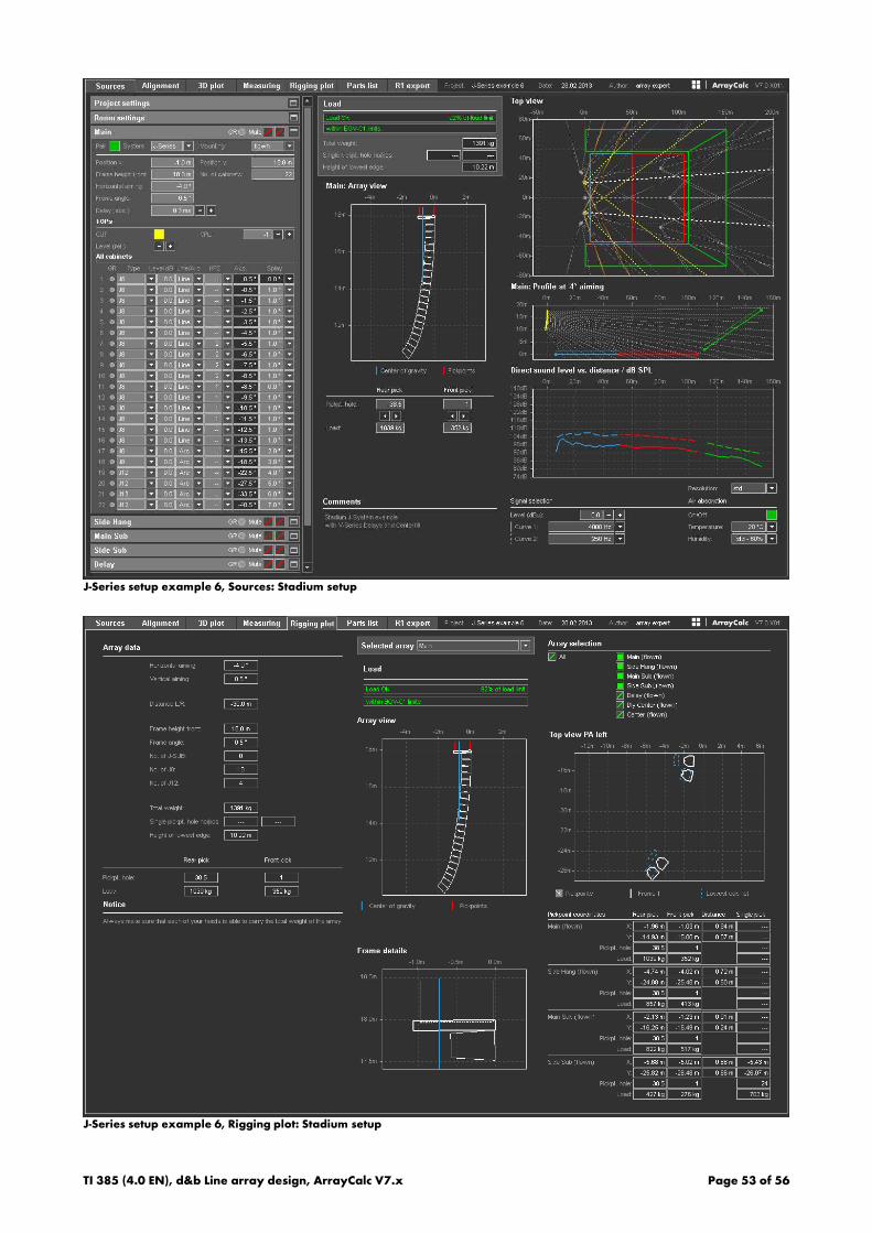
J-Series setup example 6, Sources: Stadium setup

J-Series setup example 6, Rigging plot: Stadium setup


10.5 xS/xA-Series setup examples

xS/xA-Series setup example, Sources: 8 x 10AL line array

xS/xA-Series setup example, Sources: 4 x 10S point source as delay with SPL mapping and Polar profile


xS/xA-Series setup example, Sources: 4 x 10S point source as delay with SPL mapping and Polar balloon

xS/xA-Series setup example, Sources: 6 x 5S point source as near fill with SPL mapping and Polar balloon


D5

38

5.E

N .0

3, 0

4/

20

13

© d

&b

aud

iote

chni

k G

mb

H

d&b audiotechnik GmbH, Eugen-Adolff-Strasse 134, D-71522 Backnang, Germany, Phone +49-7191-9669-0, Fax +49-7191-95 00 00