tibco statistica · tibco statistica™ installation instructions . 7 • a wide selection of...
TRANSCRIPT

TIBCO Statistica™ Quick Reference
Software Release 13.4
May 2018
Two-Second Advantage®

2 TIBCO Statistica™ Installation Instructions
Important Information SOME TIBCO SOFTWARE EMBEDS OR BUNDLES OTHER TIBCO SOFTWARE. USE OF SUCH EMBEDDED OR BUNDLED TIBCO SOFTWARE IS SOLELY TO ENABLE THE FUNCTIONALITY (OR PROVIDE LIMITED ADD- ON FUNCTIONALITY) OF THE LICENSED TIBCO SOFTWARE. THE EMBEDDED OR BUNDLED SOFTWARE IS NOT LICENSED TO BE USED OR ACCESSED BY ANY OTHER TIBCO SOFTWARE OR FOR ANY OTHER PURPOSE.
USE OF TIBCO SOFTWARE AND THIS DOCUMENT IS SUBJECT TO THE TERMS AND CONDITIONS OF A LICENSE AGREEMENT FOUND IN EITHER A SEPARATELY EXECUTED SOFTWARE LICENSE AGREEMENT, OR, IF THERE IS NO SUCH SEPARATE AGREEMENT, THE CLICKWRAP END USER LICENSE AGREEMENT WHICH IS DISPLAYED DURING DOWNLOAD OR INSTALLATION OF THE SOFTWARE (AND WHICH IS DUPLICATED IN THE LICENSE FILE) OR IF THERE IS NO SUCH SOFTWARE LICENSE AGREEMENT OR CLICKWRAP END USER LICENSE AGREEMENT, THE LICENSE(S) LOCATED IN THE “LICENSE” FILE(S) OF THE SOFTWARE. USE OF THIS DOCUMENT IS SUBJECT TO THOSE TERMS AND CONDITIONS, AND YOUR USE HEREOF SHALL CONSTITUTE ACCEPTANCE OF AND AN AGREEMENT TO BE BOUND BY THE SAME.
This document contains confidential information that is subject to U.S. and international copyright laws and treaties. No part of this document may be reproduced in any form without the written authorization of TIBCO Software Inc.
TIBCO, Better Decisioning, Data Health Check, Data Science, Decisioning Platform, Electronic Statistics Textbook, Information Bus, Live Score, Making the World Productive, Messaging Appliance, Predictive Claims Flow, Process Data Explorer, Process Tree Viewer, Rendezvous, Statistica, Statsoft, Statsoft Iberica, The Power of Now, TIB, TIBCO Rendezvous, and Two-Second Advantage are either registered trademarks or trademarks of TIBCO Software Inc. in the United States and/or other countries.
Enterprise Java Beans (EJB), Java Platform Enterprise Edition (Java EE), Java 2 Platform Enterprise Edition (J2EE), and all Java-based trademarks and logos are trademarks or registered trademarks of Oracle Corporation in the U.S. and other countries.
All other product and company names and marks mentioned in this document are the property of their respective owners and are mentioned for identification purposes only.
THIS SOFTWARE MAY BE AVAILABLE ON MULTIPLE OPERATING SYSTEMS. HOWEVER, NOT ALL OPERATING SYSTEM PLATFORMS FOR A SPECIFIC SOFTWARE VERSION ARE RELEASED AT THE SAME TIME. SEE THE README FILE FOR THE AVAILABILITY OF THIS SOFTWARE VERSION ON A SPECIFIC OPERATING SYSTEM PLATFORM.
THIS DOCUMENT IS PROVIDED “AS IS” WITHOUT WARRANTY OF ANY KIND, EITHER EXPRESS OR IMPLIED, INCLUDING, BUT NOT LIMITED TO, THE IMPLIED WARRANTIES OF MERCHANTABILITY, FITNESS FOR A PARTICULAR PURPOSE, OR NON-INFRINGEMENT.
THIS DOCUMENT COULD INCLUDE TECHNICAL INACCURACIES OR TYPOGRAPHICAL ERRORS. CHANGES ARE PERIODICALLY ADDED TO THE INFORMATION HEREIN; THESE CHANGES WILL BE INCORPORATED IN NEW EDITIONS OF THIS DOCUMENT. TIBCO SOFTWARE INC. MAY MAKE IMPROVEMENTS AND/OR CHANGES IN THE PRODUCT(S) AND/OR THE PROGRAM(S) DESCRIBED IN THIS DOCUMENT AT ANY TIME.
THE CONTENTS OF THIS DOCUMENT MAY BE MODIFIED AND/OR QUALIFIED, DIRECTLY OR INDIRECTLY, BY OTHER DOCUMENTATION WHICH ACCOMPANIES THIS SOFTWARE, INCLUDING BUT NOT LIMITED TO ANY RELEASE NOTES AND "READ ME" FILES.
Copyright © 2017 TIBCO Software Inc. All rights reserved. TIBCO Software Inc. Confidential Information

3 TIBCO Statistica™ Installation Instructions
Contents TIBCO Documentation and Support Services ........................................................................................................... 4
Chapter One Statistica: A general overview of features .............................................................................................. 5
Analytic Facilities .......................................................................................................................................................... 6
Unique Features ............................................................................................................................................................. 6
The General Philosophy of the Statistica Approach ................................................................................................. 7
Step-by-Step Examples ............................................................................................................................................... 10
Using Statistica Data Miner Recipes (SDMR) .......................................................................................................... 52
Data Management ....................................................................................................................................................... 59
Enterprise Installations ............................................................................................................................................... 79
Chapter Three: User Interface ...................................................................................................................................... 101
General Features ........................................................................................................................................................ 102
Chapter Four Six Channels for Output from Analyses ............................................................................................ 116
Overview .................................................................................................................................................................... 117
Chapter Five Statistica Documents ............................................................................................................................. 133
Workbooks ................................................................................................................................................................. 134
Chapter Six Graphs ....................................................................................................................................................... 148
Chapter Seven Customizing Statistica ....................................................................................................................... 166
Chapter Eight Statistica Visual Basic .......................................................................................................................... 171
Chapter Nine Statistica Query .................................................................................................................................... 186
Chapter Ten Programming Statistica from .NET ...................................................................................................... 190
Appendix A Statistica Enterprise Server .................................................................................................................... 194

4 TIBCO Statistica™ Installation Instructions
TIBCO Documentation and Support Services Documentation for this and other TIBCO products is available on the TIBCO Documentation site. This site is updated more frequently than any documentation that might be included with the product. To ensure that you are accessing the latest available help topics, visit: https://docs.tibco.com
How to Contact TIBCO Support For comments or problems with this manual or the software it addresses, contact TIBCO Support:
• For an overview of TIBCO Support, and information about getting started with TIBCO Support, visit this site: http://www.tibco.com/services/support
• If you already have a valid maintenance or support contract, visit this site: https://support.tibco.com Entry to this site requires a user name and password. If you do not have a user name, you can request one.
How to Join TIBCO Community TIBCOmmunity is an online destination for TIBCO customers, partners, and resident experts. It is a place to share and access the collective experience of the TIBCO community.
TIBCOmmunity offers forums, blogs, and access to a variety of resources. To register, go to the following web address:
https://www.tibcommunity.com
TIBCO Community is an online destination for TIBCO customers, partners, and resident experts. It is a place to share and access the collective experience of the TIBCO community.
TIBCO Community offers forums, blogs, and access to a variety of resources. To register, go to the following web address: https://community.tibco.com

5 TIBCO Statistica™ Installation Instructions
Chapter One Statistica: A general overview of features

6 TIBCO Statistica™ Installation Instructions
Statistica is a comprehensive analytic, research, and business intelligence tool. It is an integrated data management, analysis, mining, visualization, and custom application development system featuring a wide selection of basic and advanced analytic procedures for business, data mining, science, and engineering applications.
Analytic Facilities Statistica includes not only general purpose analytic, graphical, and database management procedures, but also comprehensive implementations of specialized methods for data analysis (such as predictive data mining; business, social sciences, and biomedical research; or engineering applications). All analytic tools offered in the Statistica line of software are available as part of an integrated package. These tools can be controlled through a selection of alternative user interfaces including:
• A highly optimized interactive user interface (with options to execute Statistica from within Microsoft Office and other applications),
• A complete thin-client, browser-based user interface (in Statistica Enterprise Server) that enables you to offload time-consuming tasks to the server and work collaboratively, and
• A comprehensive, industry standard, .NET-compatible programming interface (including the built-in, .NET-compatible Visual Basic), offering access to more than 14,000 externally callable functions.
Interactive user interfaces can be easily automated via macros and customized using a variety of methods, and they are recordable in the form of industry standard VB scripts. The built-in development environment can be used to interface Statistica with other applications and enterprise-wide infrastructures or to build custom extensions of any complexity, from simple shortcuts to advanced, large-scale development projects.
Unique Features Some of the unique features of the Statistica line of software include:
• the breadth of selection and comprehensiveness of implementation of analytical procedures,
• the unparalleled selection, quality, and customizability of graphics integrated seamlessly with every computational procedure,
• a selection of efficient and user-friendly user interfaces, • the ease of customizability using the truly open architecture compatible with virtually
all enterprise and development environments (including .NET), that exposes Statistica’s more than 14,000 functions,

7 TIBCO Statistica™ Installation Instructions
• a wide selection of advanced software technologies that is responsible for Statistica’s practically unlimited capacity, performance (speed, responsiveness), and application customization options,
• Native R scripts can be run directly within Statistica and R output can be retrieved as native Statistica Spreadsheets and Graphs.
One of the most unique and important features of the Statistica family of applications is that these technologies enable even inexperienced users to tailor Statistica to their specific preferences. You can customize practically every aspect of Statistica, including even the low- level procedures of its user interface. The same version of Statistica can be used:
• By novices to perform routine tasks using the default analysis Startup dialog Quick tab (containing just a few, self-explanatory buttons), or even by accessing Statistica with their Web browsers (and a highly simplified “front end”), and
• By experienced analysts, professional statisticians, and advanced application developers who can integrate any of Statistica’s highly optimized procedures (more than 14,000 functions) into custom applications or computing environments, using any of the cutting edge .NET and Web-compatible technologies.
The General Philosophy of the Statistica Approach Statistica’s default configuration (its general user interface and system options) is a result of years of listening carefully to our users.
We have received feedback from tens of thousands of our users, representing hundreds of thousands of our users from all continents and, practically speaking, all walks of life. One of the most important facts that we have learned from these users is how different their needs and preferences are (both across individuals and projects or applications). In order to meet those differentiated needs, Statistica is designed to offer perhaps one of the most flexible and easily customizable user interfaces of any contemporary application.
Although Statistica provides access to a powerful arsenal of advanced software technologies, you do not even need to know about them, because they are designed to work automatically and intuitively. A novice user may never see more than a few self-explanatory buttons.
Advanced options, however, are only one tab or mouse click away. Practically every aspect of Statistica (from the startup configuration, to the way the output is generated and managed by the system, to how Statistica prompts you to choose your next step) can be changed with a mouse click. Moreover, Statistica remembers your selections until you change your mind. Practically all dialogs used to select an analysis or perform a routine operation can be easily replaced (such as simplified, enhanced, or combined with custom, user-designed procedures). Statistica will always look and work the way you want.

8 TIBCO Statistica™ Installation Instructions
Software Technology (A Technical Note) The performance, customizability, and wide selection of options that can be tailored to your needs mentioned in the previous section would not be possible if Statistica did not feature the advanced technologies that drive all functions of the application.
Statistica uses and/or supports virtually all the relevant leading edge software technologies available today. Every one of the more than 14,000 Statistica functions is accessible to external applications. Practically no limitations are imposed in terms of either the amount or complexity of data that can be stored and accessed.
Statistica also is optimized for Web and multimedia applications. Computational and graphics procedures are driven by countless proprietary optimizations such as, for example, the quadruple precision computational technology that enables us to overcome the limitations of the IEEE floating point storage standards and delivers computational accuracy normally found only in designated math applications (that feature arbitrary-precision options) but not in high volume data processing applications such as statistical or data mining programs.
As a result, Statistica offers unmatched speed, numerical precision, and responsiveness, which is aided by multithreading (and the advanced supercomputer-like distributed/parallel processing architecture offered in the Client-Server version, such as Statistica Enterprise Server).
Data access is based on a flexible streaming technology that enables Statistica to work effortlessly with both the simple input data files stored on the local drive and queries of multidimensional databases containing terabytes of data and stored in remote data warehouses and processed in-place (such as without having to import them to a local storage; this feature is available in enterprise versions of Statistica).
For example, you can simultaneously run multiple instances of Statistica [in any combination of local, network, and Client-Server (Web-based) environments], each running multiple analyses of data from multiple and simultaneously open input data files and queries, and the results can be organized into separate projects. Statistica’s input and output data files and graphs can be of practically unlimited size, comprising hierarchies of documents of various types. The output can be directed to a multitude of output channels such as multimedia tables, high performance workbooks, reports (including .pdf files and Microsoft Office documents), and the Internet, as well as the optional Statistica Document Management System, which can be seamlessly integrated with any Statistica application.
Web Enablement One of the unique features of the Statistica family of applications is that it is fully Web enabled, and if Statistica Enterprise Server is installed, you can not only offload time-consuming tasks to the server, but also access the comprehensive functionality of the Statistica system using a thin-client (browser) interface.

9 TIBCO Statistica™ Installation Instructions
This includes the option to execute prepared scripts and a plethora of interactive functionality, including such operations as interactively building predictive data mining models by dragging arrows in the interactive workspace of Statistica Data Miner (using only the browser, without any client software installed).
Note that most features described in this manual are available in all Statistica products, although some sections of the manual refer only to specific products such as the Statistica Enterprise Server facilities or the Statistica Data Miner line of products.
Record of Recognition We are pleased to report that, as of this printing, Statistica has received the highest rating in every published independent comparative review in which it has been featured. In the history of the software industry, very few products have ever achieved such a record.
For more information about Statistica’s record of recognition, please visit our Web site at http://statistica.io/

10 TIBCO Statistica™ Installation Instructions
Chapter Two Step-by-Step Examples

11 TIBCO Statistica™ Installation Instructions
Analytics
Example 1: Correlations Starting Statistica. After installing Statistica, you can start the program by selecting Statistica from the Windows Start - All Programs submenu.
When you start Statistica for the first time, the User Interface dialog is displayed,
To create more space in the application window, you can minimize the ribbon bar. Either double-click on the selected tab header, or right-click on the right side of the row of tabs and from the shortcut menu, select Minimize the Ribbon.
After you click OK in the User Interface dialog, the Welcome to Statistica dialog is displayed, which contains options that are useful to access common functions in Statistica.
If you prefer, you can select the Don’t show this dialog again check box located near the bottom of the dialog, and this dialog will not be displayed when you start Statistica. Depending on the version of Statistica you have, there may be other dialogs displayed as well.
Customization of Statistica. Practically all aspects of the behavior and appearance of Statistica (even many elementary features illustrated in this example, such as where output is directed) can be permanently customized to match your preferences.
For example, even the first step (opening Statistica) can be customized; you can change the default full-screen opening mode, the appearance of the data spreadsheet, and many other aspects of Statistica, which will be illustrated throughout this manual.
Selecting a data file. For this example, open Adstudy.sta: on the Home tab in the File group, click the Open arrow. From the drop-down menu, select Open Examples to display the Open a Statistica Data File dialog. Double-click on the Datasets folder, and double-click on Adstudy. You can also open data files three ways:
1. Select Open Document from the Open drop-down menu to display the Open dialog where you can browse to the appropriate location.
2. Click the button located on each Startup Panel (the first dialog displayed when starting analysis or graph specifications).
3. Click the folder icon above Open on the Home tab.

12 TIBCO Statistica™ Installation Instructions
Data spreadsheets (multimedia tables). Statistica data files are displayed in a spreadsheet (such as one spreadsheet is one data file). All Statistica Spreadsheets are displayed using Statistica’s powerful multimedia table technology, and they can contain not only practically unlimited amounts of data, but also sound, video, embedded documents, automation scripts, and custom user interfaces.
It is possible to have more than one data spreadsheet open at a time (with each spreadsheet connected to a different analysis).
Data management facilities are available on the Data tab, which is displayed whenever a spreadsheet is open. Commands on the tabs are organized in logical groups; for example, the Data tab contains the Transformations, Cases, Variables, Manage, and Mode groups.
All the commands on the ribbon bar and classic menus are described in Statistica Help; point to (highlight) a command, and press F1 on your keyboard to display the respective Help topic.
Variable specifications. The variable (column) headers in the spreadsheet contain the variable names. Double-click on the first variable header – GENDER – to display its Variable specifications dialog.
Spreadsheet formulas. Using the options in this dialog, you can change the variable name and/or format, enter a formula to recalculate the values of the variable, etc. If the entry in the Long name (label or formula with Functions) box starts with an equal sign (=), Statistica interprets it as a formula [a comment can follow after a semicolon (;)].
For example, if you enter into the Long name… box (of variable one) =(v2+v3+v4)/3 or =mean(v2:v4), the current values of that variable will be replaced by the average of variables two through four, separately for each case (row) of the spreadsheet.

13 TIBCO Statistica™ Installation Instructions
Specifications of all variables can also be reviewed and edited together in a combined Variable Specifications Editor dialog, accessed by clicking the All Specs button in the Variable specifications dialog.
Shortcut menus accessed from spreadsheets. A useful feature of the spreadsheet is the list of commands available from its shortcut menus. Shortcut menus are dynamic menus that are displayed by right-clicking on an item (for example, a cell in the spreadsheet, as shown in the illustration below). The spreadsheet shortcut menus include a selection of specific data management operations and other options related to the currently selected variable (column), case (row), block of cells, or other item.
Six ways of handling output. You can customize the way output is managed in Statistica. You can direct all output to five basic channels:
• Workbooks • Stand-alone windows • Reports • Microsoft Word • The Web • SharePoint or Statistica Document Management System (SDMS)
The first four output channels listed above are controlled by the options in the Output Manager options pane of the Options dialog [accessible by selecting the Tools tab and clicking Options; in the Options dialog, select Output Manager in the tree view (the left pane) to view related specifications in the options pane (the right pane)].

14 TIBCO Statistica™ Installation Instructions
SharePoint options are located on the Home tab in the SharePoint group. Statistica Document Management System (SDMS), a complete solution for managing documents, is available from Statistica.
There are a number of ways to output to the Web, depending on the version of Statistica you have. These means for output can be used in many combinations (for example, a workbook and report simultaneously), and each output channel can be customized in a variety of ways.
Also, all output objects (spreadsheets and graphs) can contain other embedded and linked objects and documents, so Statistica output can be hierarchically organized in a variety of ways.
Calculating a correlation matrix. Now, let’s compute a correlation matrix for the variables in the Adstudy.sta data file. To display the Basic Statistics and Tables Startup Panel, select the Statistics tab, and in the Base group, click Basic Statistics,
or select Statistics - Basic Statistics/Tables from the Statistica Start menu in the lower-left corner of the screen.
StatMenu2.bmp

15 TIBCO Statistica™ Installation Instructions
At this point, ensure that a block (a group of selected cells) is not selected in the spreadsheet. To deselect a block, click in any cell in the spreadsheet. If a block is selected, Statistica assumes that the variables corresponding to the block are intentionally preselected for the analysis, and when you later click the OK or Summary button to produce the analysis results, instead of prompting you to select variables, Statistica will automatically produce the correlations for the selected block variables.
In the Basic Statistics and Tables Startup Panel (shown in the next illustration),
select Correlation matrices and click the OK button (or double-click Correlation matrices) to display the Product-Moment and Partial Correlations dialog.
Quick vs. advanced analyses. As with most analysis specification dialogs (and other types of Statistica dialogs), the Product-Moment and Partial Correlations dialog is organized by tabs according to the type of options available. Typically, at least two categories of options are available.
The Quick tab of a dialog contains the most commonly used options, enabling you to quickly specify a basic analysis without having to search through numerous options.
The Advanced tab typically contains the same options available on the Quick tab as well as a variety of less commonly used options (for example, in this case, options to save matrices, produce less commonly requested statistics, and create a variety of plots). Additional tabs are often available as well, depending on the type of analysis being specified.

16 TIBCO Statistica™ Installation Instructions
Note that in some cases, only a Quick tab is available. As with all dialogs in Statistica, you can press F1 on your keyboard or click the button in the upper-right corner to display a Help topic containing information about the options available on the currently selected tab.
The self-prompting nature of Statistica dialogs. All dialogs in Statistica follow the self- prompting dialog convention, which means that whenever you are not sure what to select next, simply click the OK button or the Summary button and Statistica will proceed to the next logical step, prompting you for the specific input needed (for example, variables to be analyzed).
Variables button. Every analysis specification dialog in Statistica contains one or more Variable buttons used to display the variable selection dialog to specify variables to be analyzed.
Variable selection dialog. For this example, click the One variable list button (or press ALT+V
on your keyboard) to display the Select the variables for the analysis dialog. Note that the variable selection dialog is also displayed if you click the Summary button before variables are selected.
(As mentioned previously, if a block of variables is selected in the data file, those variables will be specified automatically for the analysis, and when you click the Summary button, a correlation matrix will be produced for the variables selected in the block, not all variables in the data file.)
The variable selection dialog supports various ways of selecting variables (including the standard Windows SHIFT+click and CTRL+click conventions to select ranges and discontinuous lists of variables).

17 TIBCO Statistica™ Installation Instructions
You can also use various shortcuts and options in the variable selection dialog to review the contents of the data file. For example, you can spread the variable list to review the variables’ long names or formulas (click the Spread button), or you can zoom in on a variable (click the Zoom button) to review a sorted list of all values and descriptive statistics for the selected variable (see the next illustration).
1. For this example, select variables 1 through 10 in the variable selection dialog.
2. Click the OK button. A message will be displayed informing you that there are text variables selected.
3. Click the Continue with current selection button to return to the Product-Moment and Partial Correlations dialog.
4. Next, click the Summary button to generate a correlation matrix for the selected variables.
Note that instead of clicking the Summary button, you could have clicked the Summary: Correlations button on the Quick tab or on the Advanced tab with the same results.

18 TIBCO Statistica™ Installation Instructions
Also, depending on the defaults you have specified for handling output (in the Output Manager options pane of the Options dialog), the Correlations spreadsheet can be displayed in a report or a stand-alone window or sent to a Word document, rather than in a workbook as shown above.
Summary graphs. Statistica provides extremely flexible tools and methods for summarizing key results in graphs and/or tables.
1. For example, resume the analysis by clicking the Product-Moment and… button on the Analysis bar in the lower-left corner of the screen or by pressing CTRL+R on your keyboard.
2. Click the button to display summary graphs for each pair of variables in the correlation matrix.
These graphs not only show the scatterplot of points for each correlation, but also the distributions (histograms) for each variable, as well as the respective correlation coefficient and regression equation.
Statistica incorporates many such displays to summarize basic descriptive statistics, correlations, the results of Gage or Process capability studies, or other types of data analyses.
Results spreadsheets (multimedia tables). In addition to storing data, spreadsheets are used in Statistica to display most of the numeric output. Note that spreadsheets offer many display features and options, and in this example, significant correlations are marked with a different format to help distinguish them. By default, the color is red (in the Correlations spreadsheet, see the cell adjacent to MEASURE07 under GENDER).
Spreadsheets can hold anywhere from a short line to gigabytes of output, and they offer a variety of options to facilitate reviewing the results and visualizing them in predefined and custom-defined graphs, as will be seen later in this example.
Also, Statistica Spreadsheets can handle not only virtually unlimited amounts of data, but also video, sound, custom user interfaces, and auto-executing scripts, as well as offer virtually unlimited customization options.

19 TIBCO Statistica™ Installation Instructions
Spreadsheet options. Most spreadsheet facilities are accessible via options on the Data tab and the shortcut menus (displayed by right-clicking in the spreadsheet). You can try these options to see how they work, or you can review their descriptions by pressing the Help key (F1).
You can change all aspects of the display formats for each spreadsheet column, edit the output, or append blank cases and variables to make room for notes or output pasted from other sources.
Spreadsheets can be printed in a variety of ways (by default, in presentation-quality tables with grid lines). Also, since spreadsheets are used for input, you can easily specify an analysis using the results from a previous analysis (for example, you could use this correlation matrix to specify a multidimensional scaling analysis).
To use a results spreadsheet as an input spreadsheet, select the Input check box (located on the Data tab in the Mode group) when that spreadsheet is active.
Analysis workbooks and other output options. All results can be displayed (and stored) in stand-alone windows, reports, Word documents, or workbooks, which represent the default (and perhaps the most versatile) way of handling output from analyses.
Depending on your selections in the Output Manager (accessible by selecting the Home tab and clicking Options in the Tools group, and then selecting Output Manager, located under Analyses/Graphs), results can be put in a single workbook that holds the results from all analyses, a separate analysis workbook that holds the results (spreadsheets and graphs) from a single analysis, the workbook that contains the original data file, or a preexisting workbook.
Additionally, you can choose to have the results sent to a workbook automatically, or you can send them to the workbook yourself by clicking Add to Workbook on the Home tab in the Output group to send selected stand-alone spreadsheets or graphs to a workbook.
Output Manager. Which type of workbook you choose, or whether you choose to use a workbook, depends entirely on how you prefer to store your data and results.
• To change the output destination for the results of a particular analysis only, click the button on any analysis or graph specification dialog, and select Output to
display the Analysis/Graph Output Manager dialog.

20 TIBCO Statistica™ Installation Instructions
• To change output options for all analyses, use the (global) Output Manager (the Output Manager options pane of the Options dialog, accessible by selecting the Home tab and clicking Options in the Tools group), or select the Use global Output settings (changes here will affect the global settings) option button in the Analysis/Graph Output Manager dialog.
As with all workbooks, individual documents (for example, spreadsheets or graphs) or groups of documents can be printed, extracted, copied, and deleted from an analysis workbook.
Copy vs. Copy with Headers. Contents of spreadsheets can be copied to the Clipboard by pressing CTRL+C (which copies only the contents of the selected block). To copy the block along with its respective variable and case names, select the Edit tab, and in the Clipboard/Data group, click the Copy arrow and select Copy with Headers from the drop-down menu.
When spreadsheets are pasted into a word processor document, they will be active (in-place editable) Statistica objects, standard RTF-formatted tables, unformatted text, pictures, or HTML (depending on your choice in the Paste Special dialog of the word processor).
Printing spreadsheets. To produce a hard copy of an output spreadsheet, select the Home tab, and in the File group, click Print (or press CTRL+P) to display the Print Spreadsheet dialog, in which you specify printing options. You can also use the shortcut method of clicking the printer icon located on the Quick Access toolbar in the upper-left corner of the ribbon bar.
This shortcut method does not display the Print Spreadsheet dialog, but prints the entire current document. If you want to print a document from within a workbook, ensure that the document is selected in the workbook, and select the Selection option button in the Print Spreadsheet dialog. You can also extract a copy of the document from the workbook (drag it from the tree pane, or select the document and click Move on the Workbook tab in the Extract group) and then print it.

21 TIBCO Statistica™ Installation Instructions
Optional reports of all output. Workbooks offer perhaps the most flexible options to manage your output. In some circumstances, however, it may be useful to automatically produce a log of all results (contents of all spreadsheets and/or graphs) in a traditional word processor style report format where comments and annotations can be inserted in arbitrary locations, objects can be placed side by side, etc.
Use the options in the Output Manager to create such a report.
1. To display the Output Manager, select the Tools tab.
2. Click Options.
3. In the Options dialog, select Output Manager located under Analyses/Graphs (for global changes).
4. To display the Analysis/Graph Output Manager dialog, click the button in any analysis or graph specification dialog, and select Output (for local changes).
5. In the Output Manager options pane of the Options dialog or in the Analysis/Graph Output Manager dialog, click the Report Output arrow.
6. From the drop-down menu, select either Send to Multiple Reports (one for each Analysis/Graph), Single Report (common for all Analyses/graphs), or [Select File] (which will display the Open dialog where you can select an already established report).

22 TIBCO Statistica™ Installation Instructions
7. In the Output Manager, you can also specify the amount of supplementary information to be included with the spreadsheet results. Use the Supplementary detail option to specify either Brief ( includes only the selected spreadsheets and graphs), Medium (includes the selected spreadsheets and graphs as well as the current data file name, information on case selection conditions and case weights if any were specified, a list of all variables selected for each analysis, and the missing data values for each variable), Long [includes all information from the Medium format and the long variable labels (for example, formulas), reserving one line of output (or more) for each variable], or Comprehensive (includes all information included in the Long report format as well as a complete list of all of the text labels for each selected variable).
Interpretation of the results – Statistica Electronic Manual (Help) and the Electronic Statistics Textbook. Now let’s return to the example and the correlation matrix that has been produced.
Each of the cells of the correlation matrix represents a value (in the range of –1.00 to +1.00) that reflects the relation between the variables (see the respective variable and case headers). The higher the absolute value of the correlation coefficient, the closer the relation.
If the value is positive, the relation is positive (high values of one variable correspond to high values of the other variable; likewise, low values of one variable correspond to low values of the other variable). If the value is negative, the opposite is true (low values of one variable correspond to high values of the other variable).
To learn more about how to interpret values of correlations, you can review a comprehensive, illustrated discussion of the topic in the Electronic Manual (Statistica Help), which features the complete contents of the Statistica Electronic Statistics Textbook.
1. To display the Electronic Manual, select the Help tab.
2. In the Help group, click Help.
3. On the Search tab of the Electronic Manual, enter the respective term (for example, Correlations) into the Type in the word(s) to search for box,
4. Click the List Topics button.

23 TIBCO Statistica™ Installation Instructions
5. Select the desired topic in the Select topic box (in this case, Correlations - Introductory Overview):
Producing graphs from spreadsheets. One of the important features is the importance of scatterplots in examining correlations. For example, even very large and highly statistically significant correlation coefficients can be entirely due to one unusual data point (outlier), and if that is the case, then the correlation coefficient (even if statistically significant) would have no value to us (such as it would have no predictive validity).
Let’s examine a scatterplot that will visualize a relation between the variables and, thus, visualize a particular correlation coefficient from the table.
While examining the spreadsheet, you can view the correlations graphically, for example, to visualize the correlation between variables Measure06 and Measure04.
1. To produce a scatterplot for these two variables, right-click on the respective correlation coefficient (-0.162269).
2. In the resulting shortcut menu, select Graphs of Input Data - Scatterplot by MEASURE06 - Regression, 95% conf., as shown in the next image.
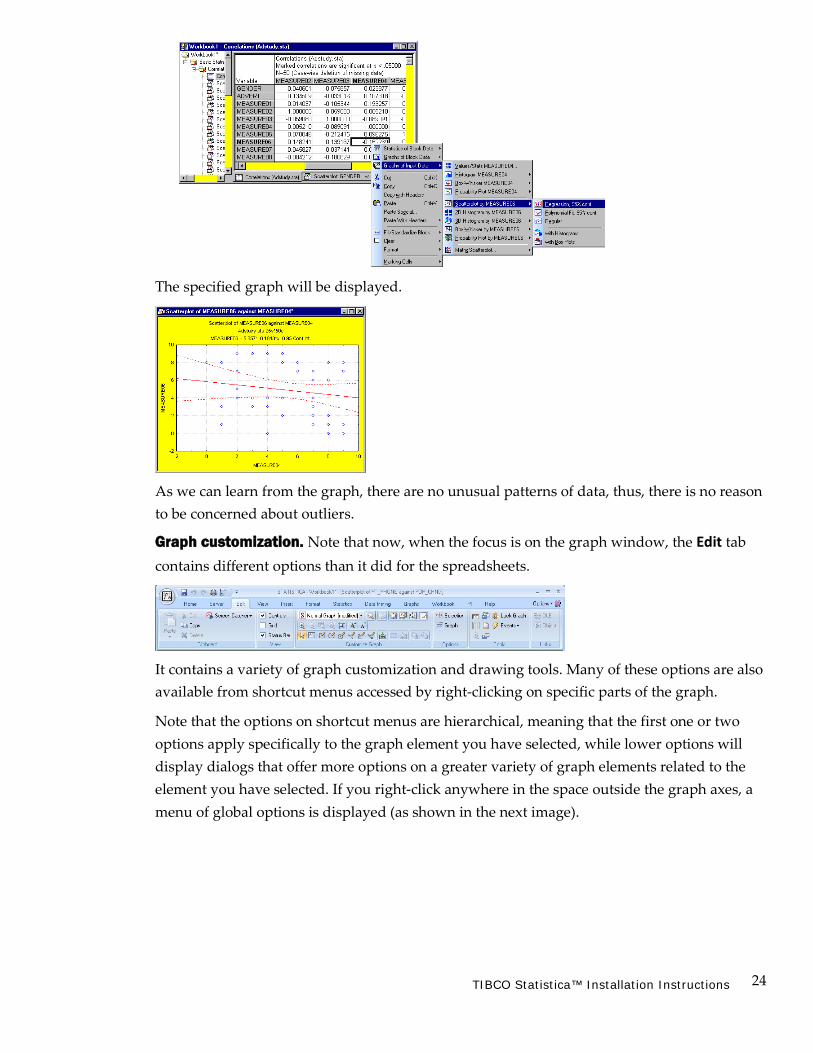
24 TIBCO Statistica™ Installation Instructions
The specified graph will be displayed.
As we can learn from the graph, there are no unusual patterns of data, thus, there is no reason to be concerned about outliers.
Graph customization. Note that now, when the focus is on the graph window, the Edit tab contains different options than it did for the spreadsheets.
It contains a variety of graph customization and drawing tools. Many of these options are also available from shortcut menus accessed by right-clicking on specific parts of the graph.
Note that the options on shortcut menus are hierarchical, meaning that the first one or two options apply specifically to the graph element you have selected, while lower options will display dialogs that offer more options on a greater variety of graph elements related to the element you have selected. If you right-click anywhere in the space outside the graph axes, a menu of global options is displayed (as shown in the next image).

25 TIBCO Statistica™ Installation Instructions
Split scrolling in spreadsheets. Spreadsheets can be split into up to four sections (panes) by dragging the split box (the small rectangle at the top of the vertical scrollbar or to the left of the horizontal scrollbar). This is useful if you have a large amount of information and you want to review results from different parts of the spreadsheet. When you move the mouse pointer to the split box, the mouse pointer changes to or . Now, to position the split, drag it to the desired position.
You can change the position of the split by dragging the split box (now located between panes) to a new position.
Note that vertically split panes scroll together when you scroll horizontally; horizontally split panes scroll together when you scroll vertically.
Drag-and-drop. Statistica supports the complete set of standard spreadsheet (Microsoft Excel- style) drag-and-drop facilities.
• In order to move a block, point to the border of the selection (the mouse pointer changes to an arrow) and drag it to the new location.
26 TIBCO Statistica™ Installation Instructions
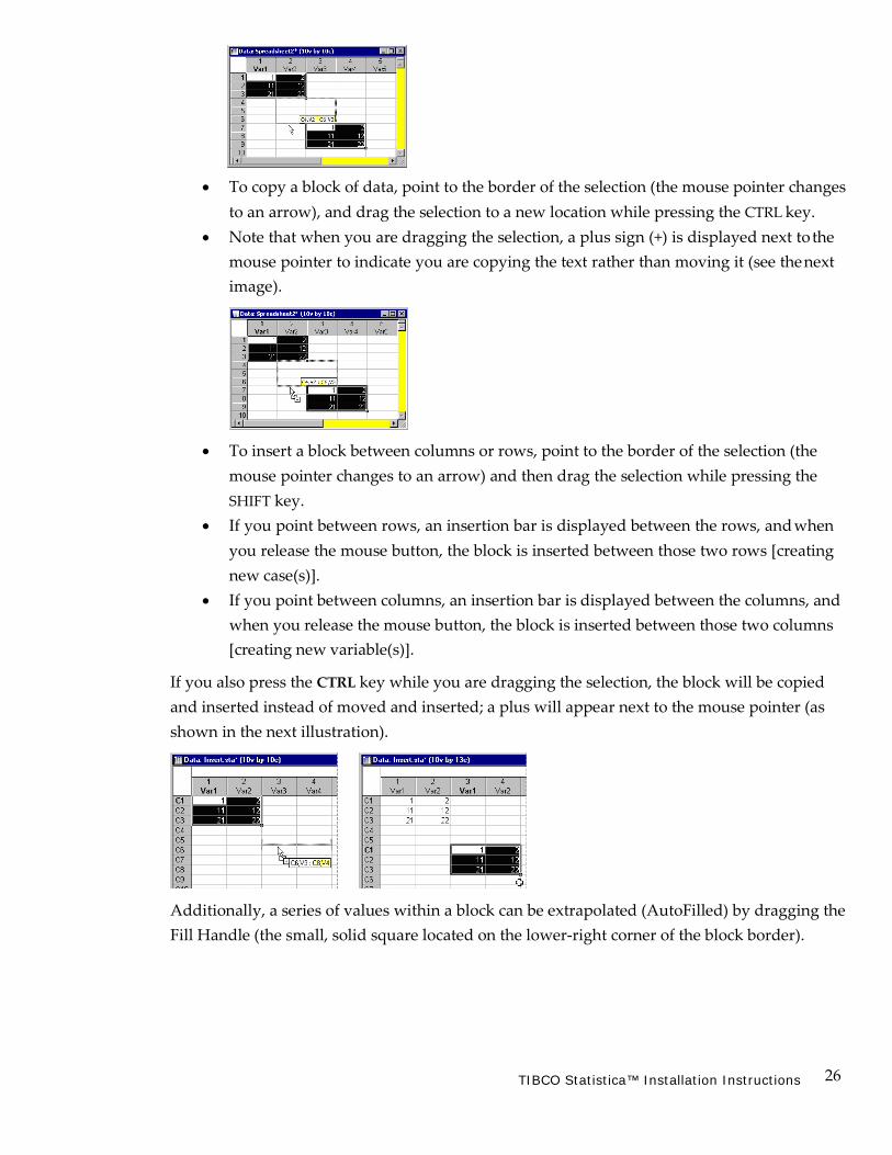
• To copy a block of data, point to the border of the selection (the mouse pointer changes
to an arrow), and drag the selection to a new location while pressing the CTRL key. • Note that when you are dragging the selection, a plus sign (+) is displayed next to the
mouse pointer to indicate you are copying the text rather than moving it (see the next image).
• To insert a block between columns or rows, point to the border of the selection (the mouse pointer changes to an arrow) and then drag the selection while pressing the SHIFT key.
• If you point between rows, an insertion bar is displayed between the rows, and when you release the mouse button, the block is inserted between those two rows [creating new case(s)].
• If you point between columns, an insertion bar is displayed between the columns, and when you release the mouse button, the block is inserted between those two columns [creating new variable(s)].
If you also press the CTRL key while you are dragging the selection, the block will be copied and inserted instead of moved and inserted; a plus will appear next to the mouse pointer (as shown in the next illustration).
Additionally, a series of values within a block can be extrapolated (AutoFilled) by dragging the Fill Handle (the small, solid square located on the lower-right corner of the block border).

27 TIBCO Statistica™ Installation Instructions
Example 2: ANOVA Calling the ANOVA module.
1. For this example of a 2 x 2 (between) x 3 (repeated measures) design, open the Adstudy.sta data file.
2. To start the ANOVA/MANOVA analysis, select the Statistics tab.
3. In the Base group, click ANOVA to display the General ANOVA/MANOVA Startup Panel.
This dialog is used to specify very simple analyses (for example, via One-way ANOVA – designs with only one between-group factor) and more complex analyses (for example, via Repeated measures ANOVA – designs with between-group factors and a within-subject factor).
Design.
1. Select Repeated measures ANOVA as the Type of analysis and Quick specs dialog as the Specification method.
2. Click the OK button in the General ANOVA/MANOVA Startup Panel to display the
ANOVA/MANOVA Repeated Measures ANOVA dialog.

28 TIBCO Statistica™ Installation Instructions
Specifying the design (variables). The first (between-group) factor is Gender (with 2 levels: Male and Female). The second (between-group) factor is Advert (with 2 levels: Pepsi and Coke). The two factors are crossed, which means that there are both Male and Female subjects in the Pepsi and Coke groups. Each of those subjects responded to three questions (this repeated measure factor will be called Response; it has three levels represented by variables Measure01, Measure02, and Measure03).
1. Click the Variables button (in the ANOVA/MANOVA Repeated Measures ANOVA dialog) to display the variable selection dialog.
2. Select Measure01 through Measure03 as dependent variables (from the Dependent variable list field) and Gender and Advert as factors [from the Categorical predictors (factors) field].
SelectVarsANOVA.bmp
3. Then click the OK button to return to the ANOVA/MANOVA Repeated Measures ANOVA dialog.
The repeated measures design. The design of the experiment that we are going to analyze can be summarized as follows:
Between-Group Between-Group Repeated Measure Factor: Response
Factor #1: Gender Factor #2: Advert Level #1: Measure01
Level #2: Measure02
Level #3: Measure03
Subject 1 Male Pepsi 9 1 6
Subject 2 Male Coke 6 7 1 Subject 3 Female Coke 9 8 2
Specifying a repeated measures factor. The minimum necessary selections are now complete, and, if we did not want to select the repeated measures factor, we would be ready to click the OK button and see the results of the analysis.
However, for our example, we need to specify that the three dependent variables we have selected be interpreted as three levels of a repeated measures (within-subject) factor. Unless we do so, Statistica assumes that those are three different dependent variables and runs a MANOVA (such as Multivariate ANOVA).

29 TIBCO Statistica™ Installation Instructions
1. In order to define the desired repeated measures factor, click the Within effects button on the Quick tab to display the Specify within-subjects factor dialog.
Note that Statistica has suggested the selection of one repeated measures factor with 3 levels (default name R1). You can specify only one within-subject (repeated measures) factor via this dialog. To specify multiple within-subject factors, use the General Linear Models module (available in the optional Advanced Linear/Nonlinear Models package).
2. Press the F1 key on your keyboard while the Specify within-subjects factor dialog is displayed (or click the button in the upper-right corner of the dialog) to display the Electronic Manual topic that describes all options in this dialog and contains links to comprehensive discussions of repeated measures and examples of designs.
3. For this example, edit the name for the factor: in the Factor Name box, change the default R1 to RESPONSE, and click the OK button to exit the dialog.
Codes (defining the levels) for between-group factors. You do not need to manually specify codes for between-group factors [such as there is no need to instruct Statistica that variable Gender has two levels: 1 and 2 (or Male and Female)] unless you want to prevent Statistica from using, by default, all codes encountered in the selected grouping variables in the data file.
1. To enter such custom code selection, click the Factor codes button to access the Select codes for indep. vars (factors) dialog.
Before you make your selections, you can use the options in this dialog to review values of individual variables by clicking the Zoom button, scan the file, and fill in the codes fields (for example, Gender and Advert) for an individual variable or all variables, etc.
2. For now, click the OK button in the Select codes for indep. vars (factors) dialog; Statistica automatically fills in the codes fields with all distinctive values encountered in the selected variables,
and closes the dialog.
30 TIBCO Statistica™ Installation Instructions
Performing the analysis.
1. Click the OK button in the ANOVA/MANOVA Repeated Measures ANOVA dialog. The analysis is performed and the ANOVA Results dialog is displayed, which contains various output spreadsheets and graphs options.
This dialog contains several tabs that enable you to quickly locate the desired results options.
2. For example, if you want to perform planned comparisons, select the Comps tab.
3. To view residual statistics, select the Resids tab. For this example, we will only use the results options available on the Quick tab.
Reviewing ANOVA results.
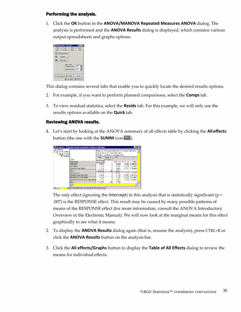
1. Let’s start by looking at the ANOVA summary of all effects table by clicking the All effects button (the one with the SUMM icon ).
The only effect (ignoring the Intercept) in this analysis that is statistically significant (p = .007) is the RESPONSE effect. This result may be caused by many possible patterns of means of the RESPONSE effect (for more information, consult the ANOVA Introductory Overview in the Electronic Manual). We will now look at the marginal means for this effect graphically to see what it means.
2. To display the ANOVA Results dialog again (that is, resume the analysis), press CTRL+R or click the ANOVA Results button on the analysis bar.
3. Click the All effects/Graphs button to display the Table of All Effects dialog to review the means for individual effects.

31 TIBCO Statistica™ Installation Instructions
This dialog contains a summary table of all effects (with most of the information you have seen in the all effects spreadsheet) and is used to review individual effects from that table in the form of the plots of the respective means (or, optionally, spreadsheets of the respective mean values).
Plot of means for a main effect.
1. In the Table of All Effects dialog, double-click on the significant main effect RESPONSE (the one marked with an asterisk in the p column) to produce the respective plot.
The graph indicates that there is a clear decreasing trend; the means for the consecutive three questions are gradually lower. Even though there are no significant interactions in this design, we will look at the highest-order interaction to examine the consistency of this strong decreasing trend across the between-group factors.
Plot of means for a three-way interaction.
1. To see the plot of the highest-order interaction, in the Table of All Effects dialog, double- click on the row marked RESPONSE*GENDER*ADVERT, representing the interaction between factors 1 (Gender), 2 (Advert), and 3 (Response).
2. An intermediate dialog, Specify the arrangement of the factors in the plot, is displayed, which is used to customize the default arrangement of factors in the graph (note that, unlike the previous plot of a simple factor, the current effect can be visualized in a variety of ways).

32 TIBCO Statistica™ Installation Instructions
3. Click the OK button to accept the default arrangement and produce the plot of means.
anovaresults3.bmp
As you can see, this pattern of means (split by the levels of the between-group factors) does not indicate any salient deviations from the overall pattern revealed in the first plot (for the main effect, RESPONSE). Now you can continue to interactively examine other effects – run post-hoc comparisons, planned comparisons, extended diagnostics, etc. – to further explore the results.
Interactive data analysis in Statistica. This example illustrates the way in which Statistica supports interactive data analysis. You are not forced to specify all output to be generated before seeing any results.
Even simple analysis designs can produce large amounts of output and countless graphs, but usually you cannot know what will be of interest until you have a chance to review the basic output. With Statistica, you can select specific types of output, interactively conduct follow-up tests, and run supplementary what-if analyses after the data are processed and basic output reviewed.
Statistica’s flexible computational procedures and wide selection of options used to visualize any combination of values from numerical output offer countless methods to explore your data and verify hypotheses.
Automating analyses (macros and Statistica Visual Basic). Any selections that you make in the course of the interactive data analysis (including both specifying the designs and choosing the output options) are automatically recorded in the industry standard Visual Basic code. You can save such macros for repeated use (you can also assign them to toolbar buttons, modify or edit them, combine them with other programs, etc.).

33 TIBCO Statistica™ Installation Instructions
Example 3: Variable Bundles Statistica offers a unique option – variable bundles – to locate a subset of data quickly and easily in a large data file. Bundles can be created to organize large sets of variables and to facilitate the repeated selection of the same set of variables.
1. Open EnginePerformance.sta. This data set describes the performance of large engines and contains various process parameters recorded during their manufacture. It includes 128 engines (their Efficiency, Fuel Economy, and Power as measured during testing) and 74 process parameters collected during the manufacture of each engine.
For this example, we will proceed with the premise that we often need to generate analyses in which the same set of variables is repeatedly used.
2. Select the Data tab.
3. In the Variables group, click Bundles to display the Variable Bundle Manager dialog.
4. Click the New button to display the New Bundle dialog.
5. Enter the name Production in the Bundle name field.
6. Click the OK button. The Select variables for bundle dialog is displayed, which contains all the variables in the EnginePerformance.sta data set.

34 TIBCO Statistica™ Installation Instructions
7. Select the variables Input01-Input05, Input20, Input30-Input35, and Input70.
8. Click the OK button to close the Select variables for bundle dialog and return to the Variable Bundle Manager.
• The left pane of this dialog displays the names of all bundles that have been defined for this spreadsheet (you can create numerous bundles in each spreadsheet if needed).
• The right pane displays the contents of the bundle that is currently selected in the left pane. If both of these panes are empty, no bundles have been created for this spreadsheet.
9. You can make changes to a bundle by clicking the Edit button, discard a bundle by clicking the Delete button, change the title of a bundle by clicking the Rename button, and produce a spreadsheet containing information about the bundles for the active data spreadsheet by clicking the Output to Spreadsheet button. For this example, click the OK button to accept the bundle we created and close the Variable Bundle Manager dialog.
10. Then, select the Statistics tab, and in the Base group, click Multiple Regression to display the Multiple Linear Regression Startup Panel. On the Quick tab, click the Variables button to display the variable specification dialog. Bundles are displayed in brackets and listed (in alphabetical order) at the top of the variable list.
11. In the Independent variable list, select the Production bundle to specify – with one click of the mouse button – Input01-Input05, Input 20, Input 30-Input35, and Input 70 as the independent variables for the analysis.
If you aren’t sure what variables are included in a bundle, move the mouse pointer over the bundle name in the variable selection dialog, and a ToolTip will display the variable numbers.

35 TIBCO Statistica™ Installation Instructions
Additionally, you can view the list of variables (by name) by clicking the [Bundles] button in the variable specification dialog. This displays the Variable Bundles Manager.
Note that bundles are defined for a single spreadsheet, and they are only used for variable selection. They are never listed in reports or other output.
As you can see with this example, you will save considerable time by selecting a bundle rather than looking for the correct variables to choose in a large data set.
Example 4: By-Group Analyses Statistica offers a powerful option to turn every statistical or graphics analysis into an analysis by group. When reviewing results in the results dialog of practically any analysis, or using the graphs options, you can select one or more grouping variables, and then create results for
• fll cases in the data combined • broken down by each combination of unique values in the grouping variables.
This is a very powerful tool for interactive and exploratory data analysis, allowing you to review quickly whether any patterns or specific results hold in all subgroups, samples, or strata in your data.
36 TIBCO Statistica™ Installation Instructions
For example, you may be performing a multiple regression analysis and decide to review, without exiting the current dialog, the results broken down by Gender and another grouping variable in your data. After selecting (enabling) this option (by clicking the By Group button), every time you click any of the results buttons (for example, to create a summary results spreadsheet or graph), all results are computed not only for all groups (optionally), but also for each unique combination of grouping variables that were specified (for example, by Gender and another grouping variable).
The results of the By Group analysis can be placed either in the default results workbook into their own folder, labeled with the respective by-group condition (for example, Gender=Female; Time=After1), or into the same folder with all other results.
For example, you could create multiple line plots to describe a multivariate batch process, creating a separate graph (trajectories) for each batch.
Exploring Experimental Data Using the By Group Option This example is based on the data file Tomatoes.sta, based on various methods of producing tomato plant seedlings prior to transplanting in the field.
1. Start by opening the example Tomatoes.sta data set.
2. Select the Home tab.
3. In the File group, click the Open arrow and select Open Examples from the drop-down menu to display the Open a Statistica Data File dialog.
4. Double-click on the Datasets folder, and then select and open the Statistica data set Tomatoes.sta.

37 TIBCO Statistica™ Installation Instructions
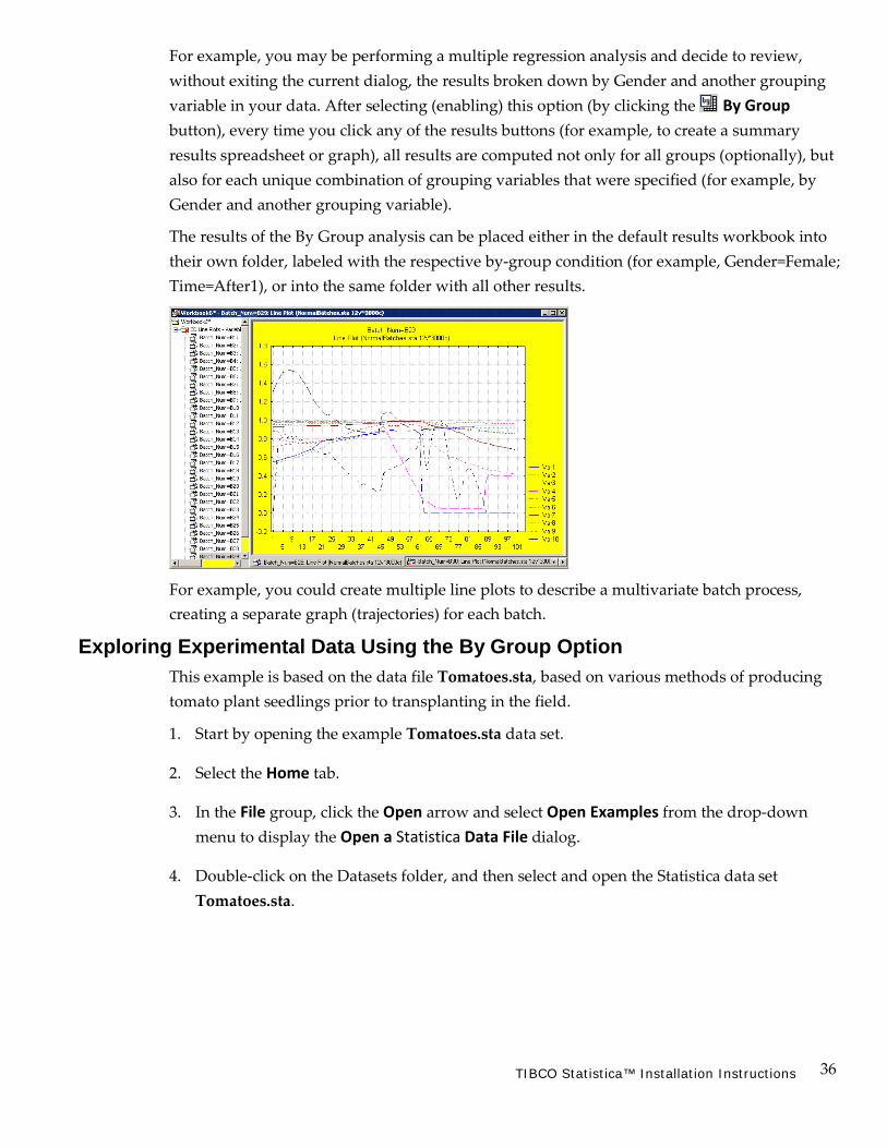
Shown here are a few rows (cases) of that data file.
Exploring Patterns by Variety This example illustrates a typical workflow as it often applies to the analysis of discrete or batch-manufacturing data, such as the goal of the analysis is to verify (graphically or analytically) that some patterns or distributions equally apply to all samples, parts, or batches.
We will explore the effect of Production Method, Soil Condition, and Potsize on yield (Pounds), and evaluate whether any patterns hold for each Variety in the study. Instead of performing a complete analysis of variance, we will use mostly graphical methods and visual inspection.
Specifying variability plots. 1. Select the Graphs tab.
2. In the More group, click 2D.
3. From the drop-down menu, select Variability Plots to display the Variability Plot dialog.
4. Click the Variables button, and in the Select Variables for Variability Plot dialog.
5. Select POUNDS as the Dependent variable, and SOIL CONDITION, POTSIZE, and
PRODUCTION METHOD from the Grouping variable list.
Further on in the example, we will create the graph by VARIETY to illustrate the By Group features.
6. Now, click the OK button in the variable selection dialog.
38 TIBCO Statistica™ Installation Instructions
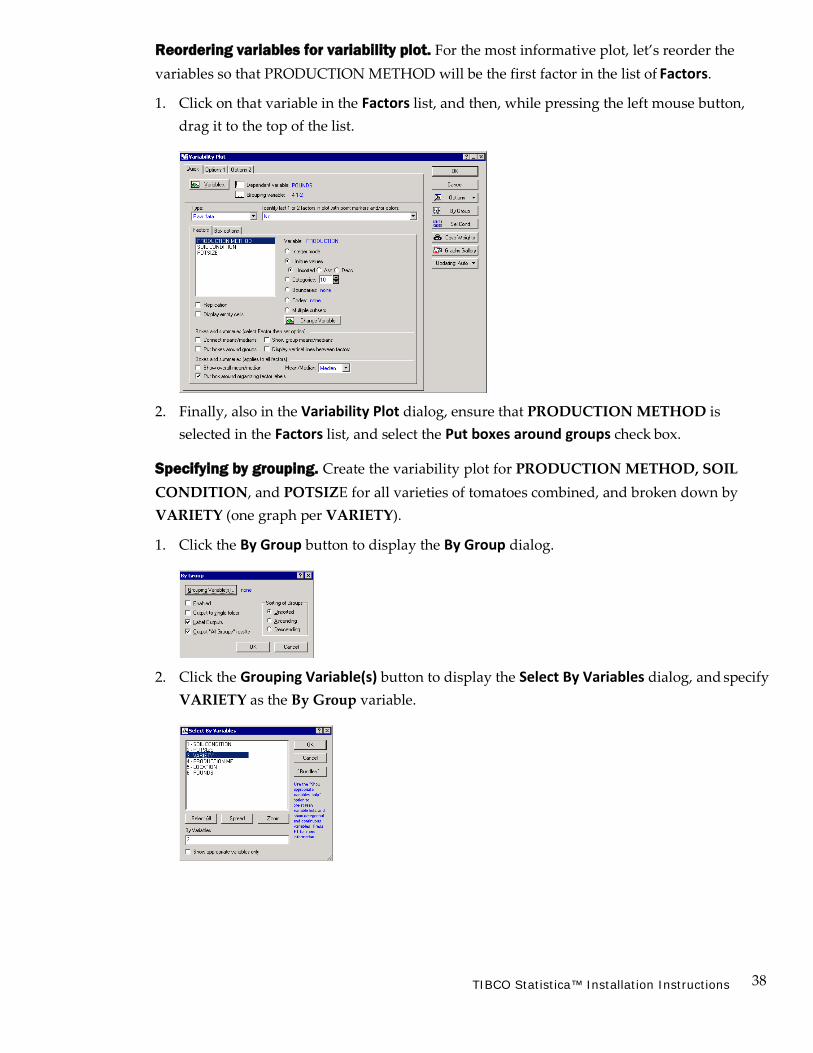
Reordering variables for variability plot. For the most informative plot, let’s reorder the variables so that PRODUCTION METHOD will be the first factor in the list of Factors.
1. Click on that variable in the Factors list, and then, while pressing the left mouse button, drag it to the top of the list.
2. Finally, also in the Variability Plot dialog, ensure that PRODUCTION METHOD is selected in the Factors list, and select the Put boxes around groups check box.
Specifying by grouping. Create the variability plot for PRODUCTION METHOD, SOIL CONDITION, and POTSIZE for all varieties of tomatoes combined, and broken down by VARIETY (one graph per VARIETY).
1. Click the By Group button to display the By Group dialog.
2. Click the Grouping Variable(s) button to display the Select By Variables dialog, and specify VARIETY as the By Group variable.

39 TIBCO Statistica™ Installation Instructions
You can specify more than one By Group variable, in which case all subsequent analyses will be performed broken down by each unique combination of values found in the By Group variables.
Reviewing the variability plots.
1. Click OK to close the Select By Variables dialog.
2. Click OK to close the By Group dialog.
3. In the Variability Plot dialog, click OK to create the graphs.
Notice how the Variability Plot is created 1) for All Groups, and 2) for each Variety (Bonny and Marglobe).
If you review these graphs carefully, you will see that the Production Method appears to make little difference (in the observed values for Pounds) for Variety=Bonny, while for Variety=Marglobe, the FibrePl method shows the least variability in values, which are generally at the higher end of the distribution of all values for variable Pounds.
Descriptive Statistics By Group Let’s next use the descriptive statistics options to further explore this.
1. Select the Statistics tab.
2. In the Base group, click Basic Statistics to display the Basic Statistics and Tables Startup Panel.
3. Select Breakdown & one-way ANOVA, and click the OK button to display the Statistics by Groups (Breakdown) dialog.
4. Click the Variables button, and in the Select the dependent variables and grouping variables dialog, specify Pounds as the Dependent variable and Production Method as the Grouping variable.
5. Then click OK to close the variable selection dialog, and click OK in the Statistics by Groups (Breakdown) dialog to display the Statistics by Groups - Results dialog.
40 TIBCO Statistica™ Installation Instructions
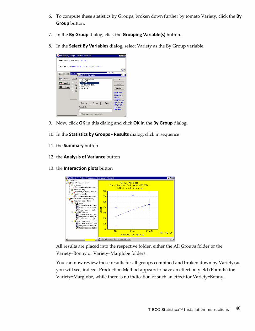
6. To compute these statistics by Groups, broken down further by tomato Variety, click the By Group button.
7. In the By Group dialog, click the Grouping Variable(s) button.
8. In the Select By Variables dialog, select Variety as the By Group variable.
9. Now, click OK in this dialog and click OK in the By Group dialog.
10. In the Statistics by Groups - Results dialog, click in sequence
11. the Summary button
12. the Analysis of Variance button
13. the Interaction plots button
All results are placed into the respective folder, either the All Groups folder or the Variety=Bonny or Variety=Marglobe folders.
You can now review these results for all groups combined and broken down by Variety; as you will see, indeed, Production Method appears to have an effect on yield (Pounds) for Variety=Marglobe, while there is no indication of such an effect for Variety=Bonny.

41 TIBCO Statistica™ Installation Instructions
Summary With Statistica, you can perform ad-hoc by-group analyses from virtually any results dialog, reviewing results for all groups combined or broken down by one or more grouping variable. This very powerful feature for exploratory data analysis can be used to compare groups and verify consistency of results across groups for any analysis.
Before concluding this topic, a few comments about the technical details regarding the implementation of this feature may be useful.
• When performing by-group analyses, as illustrated in this example, the program will actually rerun the analyses for each group (and all groups), leveraging the Statistica Visual Basic macro code that is recorded automatically during the interactive analyses, and which can be saved as macros.
• When analyzing very large data problems (for example, very large unbalanced experimental designs or complex analyses that require iterated computations before results can be displayed), the individual analyses may take up significant amounts of computing time, in particular when there are many unique groups identified in the data (for example, imagine a complex generalized linear model estimated for each of 100 groups).
• Therefore, it is generally a good idea to begin each exploratory analysis by computing simple descriptive statistics, frequency tables, and graphs to understand the structure of the data and identify the number of unique groups (combination of values in the grouping variables) in the data.
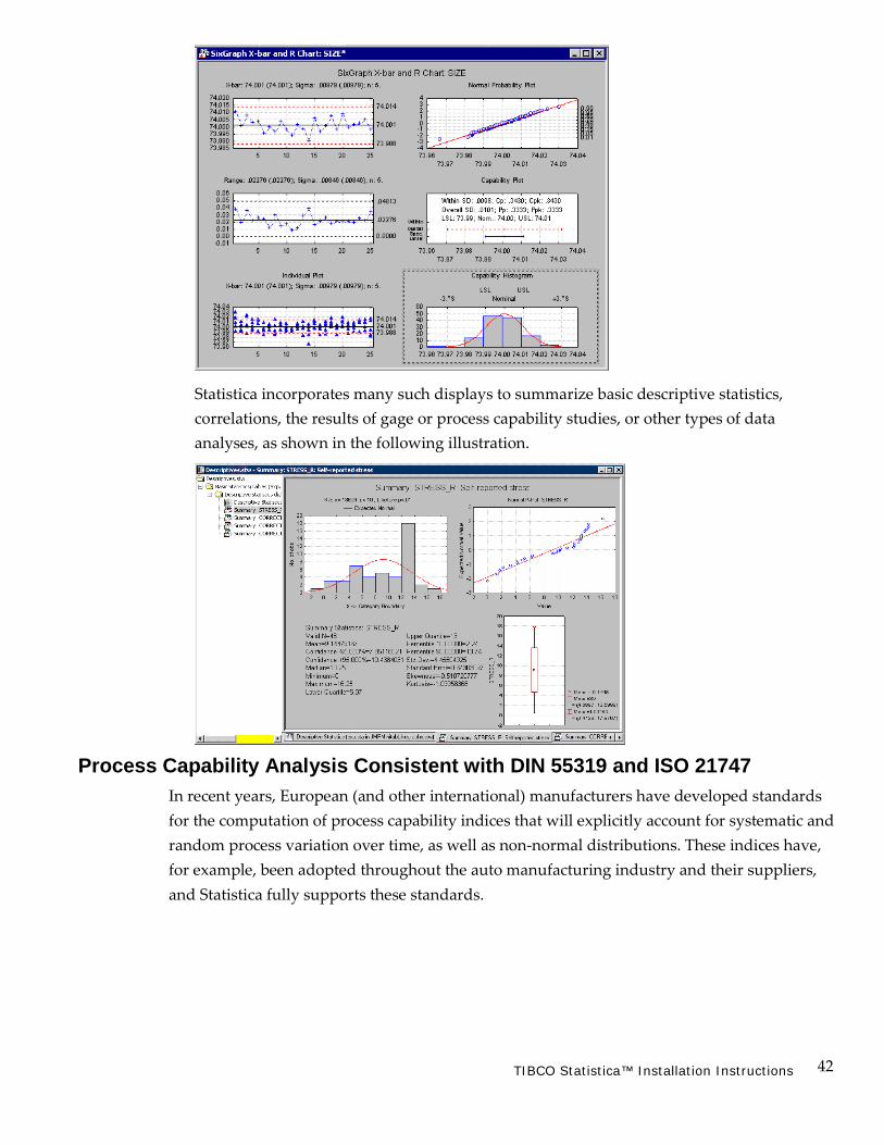
Example 5: Summary Results Panels (Quality, Process, Gage–Sixpacks) Several analyses in Statistica support summary graphs and reports arranged into a single (graphics) document. In Six Sigma and manufacturing applications, these types of displays are sometimes referred to as Quality Sixpacks because they summarize the quality of a single variable with six (or fewer) individual graphs and tables.
42 TIBCO Statistica™ Installation Instructions
Statistica incorporates many such displays to summarize basic descriptive statistics, correlations, the results of gage or process capability studies, or other types of data analyses, as shown in the following illustration.
Process Capability Analysis Consistent with DIN 55319 and ISO 21747 In recent years, European (and other international) manufacturers have developed standards for the computation of process capability indices that will explicitly account for systematic and random process variation over time, as well as non-normal distributions. These indices have, for example, been adopted throughout the auto manufacturing industry and their suppliers, and Statistica fully supports these standards.

43 TIBCO Statistica™ Installation Instructions
Process capability indices measure the number of times that the observed (normal) distribution of values can fit inside the specification limits for the respective part under consideration. Thus, these indices summarize the quality of a process to produce products or parts that are consistent with design specifications.
For example, even if a distribution of data points within each sample is Normal, if there is systematic or random variation that occurs over time as successive samples are taken, the resultant distribution of values will not be Normal. Therefore, in many cases the normal distribution-based process capability computations will not be applicable. Also, it is usually of interest to identify any time-dependent variability or trends because they can indicate machine wear or other process problems.
The following example illustrates step-by-step how to compute process capability indices consistent with these international standards, and how to create an efficient single-document summary report.
Select data. This example is based on a data set reported in Montgomery (1985, page 177, 1991, page 234). We’ll use the data file Pistons.sta that is located in Statistica’s examples directory. Specifically, we are interested in monitoring the size (diameter) of piston rings for automotive engines.
Therefore, constant samples of five observations each have been taken from the ongoing manufacturing process. As is the case in many ongoing manufacturing processes, samples are taken over time, so any variability in the process quality over time will affect the overall variability.
1. On the Home tab, click the Open arrow, and from the drop-down menu, select Open Examples to display the Open a Statistica Data File dialog
2. Open the Datasets folder, and double-click on Pistons.sta or select it and click the Open button.
Specify analysis.
1. Select the Statistics tab.
2. In the Industrial Statistics group, click Process Analysis.
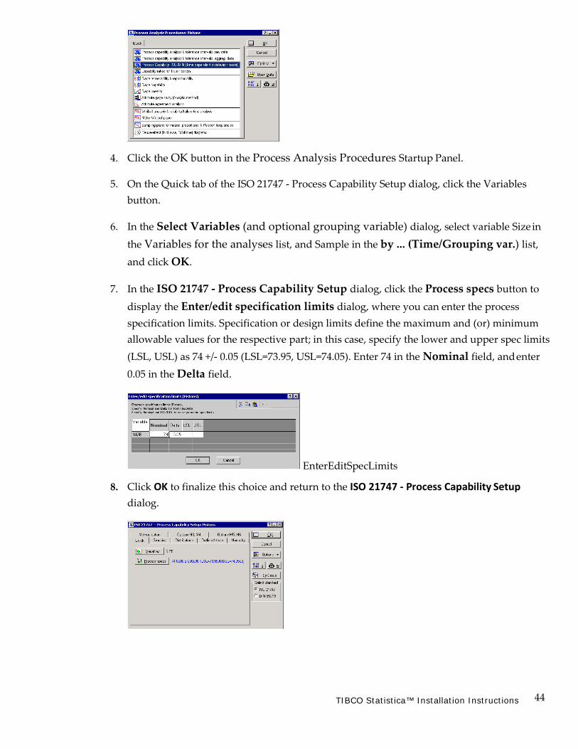
3. In the Process Analysis Procedures Startup Panel, select Process Capability ISO/DIN (Time dependent distribution model).
44 TIBCO Statistica™ Installation Instructions
4. Click the OK button in the Process Analysis Procedures Startup Panel.
5. On the Quick tab of the ISO 21747 - Process Capability Setup dialog, click the Variables button.
6. In the Select Variables (and optional grouping variable) dialog, select variable Size in
the Variables for the analyses list, and Sample in the by ... (Time/Grouping var.) list,
and click OK.
7. In the ISO 21747 - Process Capability Setup dialog, click the Process specs button to
display the Enter/edit specification limits dialog, where you can enter the process specification limits. Specification or design limits define the maximum and (or) minimum allowable values for the respective part; in this case, specify the lower and upper spec limits (LSL, USL) as 74 +/- 0.05 (LSL=73.95, USL=74.05). Enter 74 in the Nominal field, and enter 0.05 in the Delta field.
EnterEditSpecLimits
8. Click OK to finalize this choice and return to the ISO 21747 - Process Capability Setup dialog.
45 TIBCO Statistica™ Installation Instructions
In this dialog, there are numerous other options available to modify the rules that are applied to select the most appropriate distribution and time-dependent distribution model for the data so that the appropriate process capability indices can be computed.
9. Now click the OK button in the ISO 21747 - Process Capability Setup dialog to perform the analyses for variable Size.
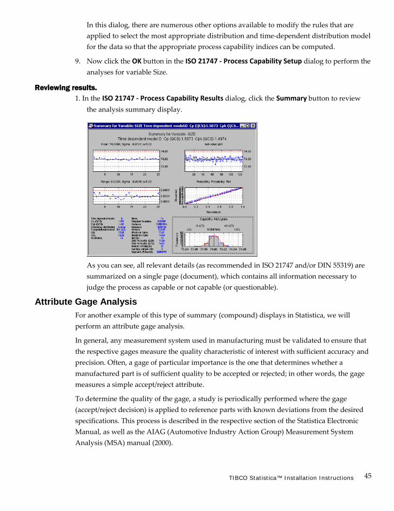
Reviewing results. 1. In the ISO 21747 - Process Capability Results dialog, click the Summary button to review
the analysis summary display.
As you can see, all relevant details (as recommended in ISO 21747 and/or DIN 55319) are summarized on a single page (document), which contains all information necessary to judge the process as capable or not capable (or questionable).
Attribute Gage Analysis For another example of this type of summary (compound) displays in Statistica, we will perform an attribute gage analysis.
In general, any measurement system used in manufacturing must be validated to ensure that the respective gages measure the quality characteristic of interest with sufficient accuracy and precision. Often, a gage of particular importance is the one that determines whether a manufactured part is of sufficient quality to be accepted or rejected; in other words, the gage measures a simple accept/reject attribute.
To determine the quality of the gage, a study is periodically performed where the gage (accept/reject decision) is applied to reference parts with known deviations from the desired specifications. This process is described in the respective section of the Statistica Electronic Manual, as well as the AIAG (Automotive Industry Action Group) Measurement System Analysis (MSA) manual (2000).

46 TIBCO Statistica™ Installation Instructions
Select data.
1. Open the AttributeGageStudy.sta data file. This file contains the data, already summarized to acceptance data, of the attribute gage study.
Specify analysis.
1. Select the Statistics tab.
2. In the Industrial Statistics group, click Process Analysis.
3. In the Process Analysis Procedures Startup Panel, select Attribute gage study (Analytic method), and click the OK button.
4. In the Attribute gage study (Analytic method) dialog, click the Variables button.
5. Select Part# in the Part numbers list, Reference in the Reference values list, and
Acceptance in the Acceptance/Response list, and then click the OK button to close this
dialog and return to the Attribute gage study (Analytic methods) dialog.
6. In the Tolerance limit for calculation group, specify -0.01 as the Lower limit, select the Display the other limit check box, and then specify 0.01 as that limit.
We are interested in evaluating the gage performance for a process or type of manufactured part that should be identified as unacceptable (should be rejected), when its real lower limit drops below -0.01 (expressed here as a deviation from the spec). In the data file, the Acceptance probabilities summarize the number of reference parts measurements, from a total of 20 such parts and measurements each, that were declared as unacceptable (such as that were rejected).
Reviewing results.
1. Now click OK in the Attribute gage study (Analytic methods) dialog.
2. In the Results dialog, click the Summary button to review the summary results.

47 TIBCO Statistica™ Installation Instructions
All important results to determine the bias and repeatability (of measurements) of the attribute gage are summarized on a single page.
Example 6: Statistica Data Miner Statistica Data Miner (SDM) is a comprehensive system for predictive modeling that offers a wide variety of analytic techniques and model building, validation, and model deployment options.
The default, and perhaps the industry standard, type of user interface provided in SDM follows the general interactive data mining workspace approach that enables users to build models by dragging icons representing steps of data acquisition, data preparation, modeling, and deployment and connect them with arrows.
The workspace user interface option in SDM represents a powerful alternative to the traditional interactive data analysis user interface, and it can be used not only as a tool for developing and testing predictive data mining modes, but also as a powerful general tool to be used for visual programming of analytic workflows for many types of analyses.
1. To open a new (blank) data mining workspace, select the Data Mining tab.
2. In the Tools group, click Workspaces and from the menu, select either New Workspace - My Procedures or New Workspace - All Procedures.

48 TIBCO Statistica™ Installation Instructions
A blank data mining workspace will be displayed.
3. Now, click on the toolbar to display the Select Data Source dialog, used to select a data file for analysis.
4. Next, the Select dependent variables and predictors dialog is displayed. Click the button to display the variable selection dialog, used to specify the dependent
variables and predictors.
5. Then, click to create analytic nodes, and connect them with arrows to specify the desired project workflow.
Overview
The following section includes a step-by-step example of Data Miner Recipes – an innovative user interface for data mining introduced by Statistica – which offers a powerful alternative to the workspace-based approach to model building, and can be used by both novices and advanced analysts.
This example pertains to Statistica Data Miner Recipes, a Statistica product that offers a wide selection of methods for predictive data mining.
A general trend in data mining is the increasing emphasis on solutions based on simple analytic processes rather than the creation of ever-more sophisticated general analytic tools. Statistica Data Miner Recipes (SDMR) offers an easy-to-use alternative to the traditional data miner workspace user interface for building predictive data mining models.
This approach provides an intuitive graphical interface to enable those with limited data mining experience to execute a recipe-like step-by-step analytic process. With these intuitive dialogs, you can perform various data mining tasks such as regression, classification, and clustering. Other recipes can be built quickly as custom solutions.

49 TIBCO Statistica™ Installation Instructions
Completed recipes can be saved and deployed as project files to score new data. The project files can be generated as C/C++ language or PMML script, or sent to Statistica Enterprise.
The SDMR user interface can also be used by advanced analysts to automate and store specific data mining algorithms.
SDMR spans the entire data mining process – from querying external databases to the final deployment of solutions – and, in general, consists of the following steps.
1. Identifies the data from which to learn
• Connects to ODBC or OLEDB compliant databases • Connects to Statistica data files
2. Cleans data and removes the redundant predictors
• Flexible and efficient methods for sampling the data (simple, stratified, systematic, etc.) • More flexible ways to identify and recode the missing data • Identification of outliers • Transform the data prior to performing the subsequent steps • Identify and eliminate redundant predictors
3. Identifies important predictors from a large pool of predictors that are strongly related to the dependent (outcome or target) variable of interest
• Feature selection for very large data sets (for example, thousands of variables) • Detection of important interactions among the predictors by using tree-based methods
4. Generates a pool of eligible models
• Leverage the comprehensive selection of cutting edge techniques for predictive data mining available in SDMR
• Offload computationally expensive tasks to Statistica Enterprise Server, freeing your local computer for other tasks
5. Performs automatic competitive evaluation of models to identify the optimum model with respect to performance and complexity
6. Deploys the model to score new data using the inbuilt efficient deployment engine
Statistica Data Miner Recipes provides the solution that maps the steps of the data mining workflow into a results-oriented user interface. From data cleaning to model validation, SDMR guides your analysis from start to finish so that you can get actionable results and answers quickly.
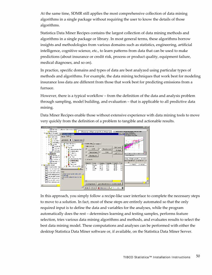
50 TIBCO Statistica™ Installation Instructions
At the same time, SDMR still applies the most comprehensive collection of data mining algorithms in a single package without requiring the user to know the details of those algorithms.
Statistica Data Miner Recipes contains the largest collection of data mining methods and algorithms in a single package or library. In most general terms, these algorithms borrow insights and methodologies from various domains such as statistics, engineering, artificial intelligence, cognitive science, etc., to learn patterns from data that can be used to make predictions (about insurance or credit risk, process or product quality, equipment failure, medical diagnoses, and so on).
In practice, specific domains and types of data are best analyzed using particular types of methods and algorithms. For example, the data mining techniques that work best for modeling insurance loss data are different from those that work best for predicting emissions from a furnace.
However, there is a typical workflow – from the definition of the data and analysis problem through sampling, model building, and evaluation – that is applicable to all predictive data mining.
Data Miner Recipes enable those without extensive experience with data mining tools to move very quickly from the definition of a problem to tangible and actionable results.
In this approach, you simply follow a recipe-like user interface to complete the necessary steps to move to a solution. In fact, most of these steps are entirely automated so that the only required input is to define the data and variables for the analyses, while the program automatically does the rest – determines learning and testing samples, performs feature selection, tries various data mining algorithms and methods, and evaluates results to select the best data mining model. These computations and analyses can be performed with either the desktop Statistica Data Miner software or, if available, on the Statistica Data Miner Server.

51 TIBCO Statistica™ Installation Instructions
Data Miner Recipes Project Files When you save a Data Miner Recipes project at any stage of completion, two separate files are created:
• A Data Miner Recipes file with the file name extension .dmrproj • A Statistica Workbook file by the same name, but with the file name extension .stw,
containing results and detailed information for each step of the recipe
It is important that both files reside in the same file directory. So, if you want to copy a Data Miner Recipe project called MyDataMinerProject to a new file directory, email it to a colleague, or check it into the Statistica Document Management System, then both files – MyDataMinerProject.dmrproj and MyDataMinerProject.stw – must be copied to the new destination.
Following are additional details about these two files.
Data Miner Recipes file (.dmrproj). The Data Miner Recipes are XML (extensible markup language) format files that contain all information regarding users’ choices (or choices automatically made by the program), including:
• Data file information (or data connection information) • Variable selections and variable metadata (for example, defining continuous and
categorical predictors and outcomes) • Choices about data preprocessing steps (for example, missing data handling, filtering
of duplicate records, transformations, etc.) • Final variable selections based on the application of feature selection algorithms • Results from model building and final evaluation and choices of models • All information necessary to deploy predictive models and to predict new cases (for
example, to score databases, compute component scores, inferred sensor values, predicted risk or failure probabilities, etc.)
Therefore, when deploying Data Miner Recipes to the Statistica Enterprise software to automatically compute predicted values in an enterprise application (automated credit scoring, multivariate control charting and failure analysis, etc.), all information necessary to compute predicted values, classifications, or classification probabilities (for example, probability of default, loss) is contained inside these XML format files.
Data Miner Recipes Workbook file (.stw). These files contain detailed information describing the results for each step.
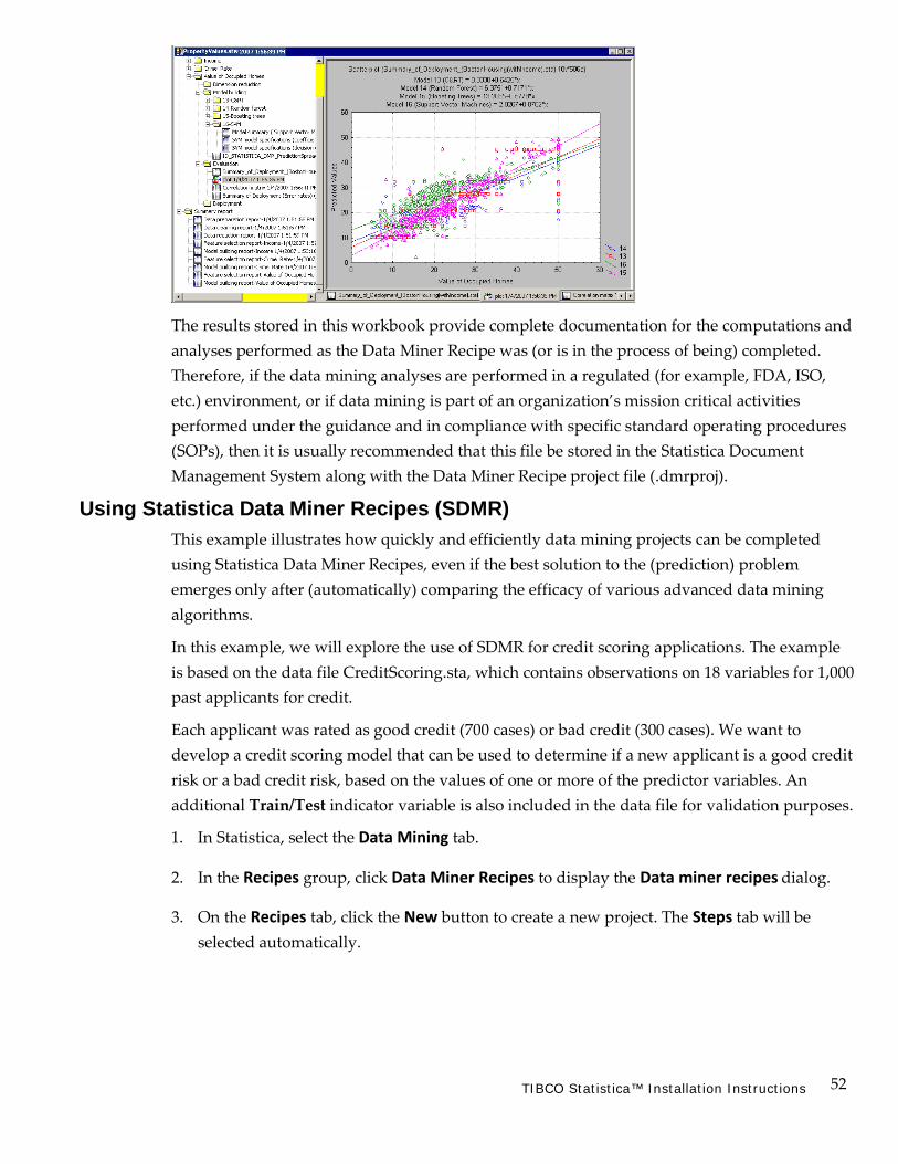
52 TIBCO Statistica™ Installation Instructions
The results stored in this workbook provide complete documentation for the computations and analyses performed as the Data Miner Recipe was (or is in the process of being) completed. Therefore, if the data mining analyses are performed in a regulated (for example, FDA, ISO, etc.) environment, or if data mining is part of an organization’s mission critical activities performed under the guidance and in compliance with specific standard operating procedures (SOPs), then it is usually recommended that this file be stored in the Statistica Document Management System along with the Data Miner Recipe project file (.dmrproj).
Using Statistica Data Miner Recipes (SDMR) This example illustrates how quickly and efficiently data mining projects can be completed using Statistica Data Miner Recipes, even if the best solution to the (prediction) problem emerges only after (automatically) comparing the efficacy of various advanced data mining algorithms.
In this example, we will explore the use of SDMR for credit scoring applications. The example is based on the data file CreditScoring.sta, which contains observations on 18 variables for 1,000 past applicants for credit.
Each applicant was rated as good credit (700 cases) or bad credit (300 cases). We want to develop a credit scoring model that can be used to determine if a new applicant is a good credit risk or a bad credit risk, based on the values of one or more of the predictor variables. An additional Train/Test indicator variable is also included in the data file for validation purposes.
1. In Statistica, select the Data Mining tab.
2. In the Recipes group, click Data Miner Recipes to display the Data miner recipes dialog.
3. On the Recipes tab, click the New button to create a new project. The Steps tab will be selected automatically.

53 TIBCO Statistica™ Installation Instructions
The step-node panel is located in the upper-left area of the Steps tab. It contains four major nodes: Data preparation, Data for analysis, Data redundancy, and Target variable.
Nodes (steps). Each node (or step) can exist in one of four states, depending on whether all required options have been specified. Each state is represented by an icon: a red indicates a wait state, meaning a step cannot be started because it is dependent on a previous step that has not been completed; a yellow indicates a ready state, meaning you are ready to start the step because previous steps have been completed; a green indicates a completed step. Note that you must click the Next step button to change the yellow (ready state) to the green (completed state).
The change will be made only if the step has been successfully completed (such as all required information has been specified). Lastly, if you have opened a data set and selected variables, and you do not want to proceed step by step through all the options, you can select the Configure all steps check box on the Steps tab. The steps will now be represented by a navy icon.
You can select any of the steps and modify the options, or you can leave all options at their defaults. Then, click the Next step arrow, and from the drop-down list, select Run to completion. Statistica Data Miner Recipes will run the analysis and create the model results.
Options tab. The Options tab of Statistica Data Miner Recipes is used to set global options for recipes using very large data files. Options include specifications for sampling and for maximum file size to save in the Project Workbook. Since most of these options are applied to the Data preparation step, they should be set prior to starting work on a new recipe. Modifications to the values on this tab apply only to the current recipe unless you click the Save defaults button.
Data Preparation Connecting data. On the Data preparation tab, click the Open/Connect data file button.

54 TIBCO Statistica™ Installation Instructions
1. In the Select Data Source dialog, click the Files button to browse to and open the CreditScoring.sta data file (located in the Datasets folder installed with Statistica).
2. If the data file is already open, it will be listed in the Open Spreadsheet Documents folder; double-click it to open it, or select it and click the OK button.
3. On the Data preparation tab, click the Select variables button, and in the Select variables dialog, select:
Variable 1 - (Credit Rating) as the Target, categorical variable,
Variables 3, 6, and 14 as Input, continuous predictors
Variables 2, 4-5, 7-13, and 15-18 as Input, categorical predictors, and
Variable 19 - TrainTest as the Testing sample variable.
4. Then, click the OK button.
5. Select the Advanced tab in the Data miner recipes dialog, and select the Use sample data check box.
6. Select the Stratified random sampling option button as the sampling strategy to ensure that
each class of the dependent variable Credit Rating is represented with approximately equal numbers of cases in train and validation sets.
7. Then click the More options button to display the Stratified sampling dialog.
8. Click the Strata variables button, select Credit Rating as the strata variable, and click OK in this dialog and in the Stratified sampling dialog.
9. Click the Next step button for the Data preparation step to ensure that this step has been successfully completed (in the step-node panel next to Data preparation, the yellow changes to a green ).
Data for Analysis After the Data preparation step is completed, the Data for analysis step will be selected automatically.

55 TIBCO Statistica™ Installation Instructions
1. On the Data for analysis tab, click the Select testing sample button, and in the Testing Sample Specifications dialog, select the Variable option button.
2. Verify that the category (value) Train is entered in the Code for training sample field and Test is entered in the Code for testing sample field.
3. Then, click the OK button. The models will be fitted using the training sample and evaluated using the observations in the testing sample. By using observations that did not participate in the model fitting computations, the goodness-of-fit statistics computed for (predicted values derived from) the different data mining models (algorithms) can be used to evaluate the predictive validity of each model and, hence, can be used to compare models and to choose one or more over others.
Descriptive statistics. This step will also compute descriptive statistics for all variables selected in the analysis. Descriptive stats provide useful information about ranges and distributions of the data used for the project.
1. Click the Next step button to ensure that this step is successfully complete.
Data Redundancy Now, the Data redundancy step will be selected. The purpose of this step is to eliminate highly redundant predictors. For example, if the data set contained two measures for weight, one in kilogram the other in pounds, then those two measures would be redundant.
1. On the Data redundancy tab, select the Correlation coefficient option button, and specify the Criterion value as 0.8.
2. Click the Next step button to eliminate the redundant predictors that are highly correlated (r≥0.8). Since there is no redundancy in the data set we are using in this example, a message dialog will be displayed stating this.
3. Click the OK button. The data cleaning and preprocessing for model building is now complete.
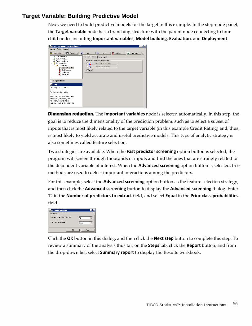
56 TIBCO Statistica™ Installation Instructions
Target Variable: Building Predictive Model Next, we need to build predictive models for the target in this example. In the step-node panel, the Target variable node has a branching structure with the parent node connecting to four child nodes including Important variables, Model building, Evaluation, and Deployment.
Dimension reduction. The Important variables node is selected automatically. In this step, the goal is to reduce the dimensionality of the prediction problem, such as to select a subset of inputs that is most likely related to the target variable (in this example Credit Rating) and, thus, is most likely to yield accurate and useful predictive models. This type of analytic strategy is also sometimes called feature selection.
Two strategies are available. When the Fast predictor screening option button is selected, the program will screen through thousands of inputs and find the ones that are strongly related to the dependent variable of interest. When the Advanced screening option button is selected, tree methods are used to detect important interactions among the predictors.
For this example, select the Advanced screening option button as the feature selection strategy, and then click the Advanced screening button to display the Advanced screening dialog. Enter 12 in the Number of predictors to extract field, and select Equal in the Prior class probabilities field.
Click the OK button in this dialog, and then click the Next step button to complete this step. To review a summary of the analysis thus far, on the Steps tab, click the Report button, and from the drop-down list, select Summary report to display the Results workbook.

57 TIBCO Statistica™ Installation Instructions
These predictors will be further examined using various cutting-edge data mining and machine learning algorithms available in SDMR.
Building models. The Data miner recipes dialog was minimized so that you could see the Results workbook. Click the Data miner recipes button located on the Analysis Bar (in the lower-left corner of the application) to display the dialog again. Now, the Model building node is selected. In this step, you can build a variety of models for the selected inputs. On the Model building tab, C&RT, Boosted tree, and Neural network are selected by default as the models or algorithms that will automatically be tried against the data.
The computations for building predictive models can be performed either locally (on your computer) or on the Statistica Enterprise Server. However, the latter option is available only if you have a valid Statistica Enterprise Server account and you are connected to the server installation at your site. For this example, click the Build model button to perform the computations locally on your computer. This will take a few moments; when finished, click the Next step button to complete this step.
Evaluating and selecting models. Now, the Evaluation node is selected. On the Evaluation tab in the Select model(s) field, ensure that all models are selected (each check box is selected). Click the Evaluate models button to perform the competitive evaluation of models for identifying the best performing model in terms of performance in the validation sample.
Notice that the Boosting Trees model has the minimum error rate of 31.48%. In other words, 68.52% of the cases in the validation sample are correctly predicted by this model. Note that your results may vary slightly because these advanced data mining methods randomly split the data into subsets during training to produce reliable estimates of the error rates.
The following spreadsheet shows the classification performance of the best model on the validation data set. The columns represent the predicted class frequencies, as predicted by the Boosting Trees model, and the rows represent the actual or observed classes in the validation sample.

58 TIBCO Statistica™ Installation Instructions
In this matrix, you can see that this model predicted 68 out of 103 “bad credit risks” correctly, but misclassified 35 of them. This information is usually much more informative than the overall misclassification rate, which simply tells us that the overall accuracy is 68.52%.
Display the Data miner recipes dialog again, and click the Next step button. A message is displayed with instructions to select only one model for deployment. Click OK, and clear the check boxes adjacent to C&RT and Neural network. We will deploy the Boosting Trees model that gave us the best predictive accuracy on the test sample. Now, click the Next step button again.
Deployment The final Deployment step involves using the best model and applying it to new data in order to predict the “good or bad” customers.
This step also provides the option for writing back the scoring information (classification probabilities computed by the best model, predicted classification, etc.) to the original input data file or database. This is extremely useful for deploying models on very large data sets to score databases.
On the Deployment tab, click the Data file for deployment button and open the CreditScoring.sta data file (located in the Datasets folder installed with Statistica). For demonstration purposes, we are using the same data file for deployment of the best model.

59 TIBCO Statistica™ Installation Instructions
Click the Next step button to score this data file using the best model. The scored file with classifications and prediction probabilities (titled Summary of Deployment) is located in the Deployment folder in the project workbook as shown below.
Summary The purpose of this example is to demonstrate the efficiency of the data miner workflow implemented in Statistica Data Miner Recipes. With only a few clicks, the program will take you through the complete analytic process - from the definition of input data and analysis problem, through data cleaning and preparation and model building, all the way to final model selection and deployment.
Even though most of the computational complexities of data mining are resolved automatically in Statistica Data Miner Recipes, which enables you to move from problem definition to a solution very quickly even if you are a novice, the program will apply and try a large number of advanced data mining algorithms and automatically determine which approach is most successful.
Thus, the Statistica Data Miner Recipes methodology and user interface enables you to leverage the largest collection of data mining algorithms in a single package to solve your problems.
Data Management Example 1: Spreadsheet Formulas and Batch Formulas
You can define new variables for Statistica Spreadsheets in terms of other variables, sometimes referred to as variable transformations. Additionally you can verify data, transform data, and recode data on a single variable (as opposed to a set of transformation formulas, such as batch formulas). This is accomplished with spreadsheet formulas.
To access spreadsheet formulas, double-click on a variable header in a Statistica Spreadsheet to display the Variable specification dialog.
60 TIBCO Statistica™ Installation Instructions
The formula is entered into the Long name (label or formula with Functions) field (also called the formula editor) located at the bottom of the dialog. When you enter a long variable name in the formula editor that starts with an equal sign, Statistica recognizes it as a formula and will verify it for formal correctness.
The formula can reference other variables either by name (MEASURE01, TIME), or by absolute variable number using the Vx syntax, where x is the absolute variable number. For example, V3 is variable number 3. V0 has special meaning, and refers to the current case number.
Spreadsheet formulas are evaluated a case (row) at a time. For each case in the spreadsheet, the formula is evaluated, and references to the other variables are substituted with their values from the current case.
In Statistica, random access spreadsheet functions enable the formula to access variable values from other cases. A common example of this is the Lag function, which will reference a variable, and lag it forward or backward a certain number of cases.
The following table lists several spreadsheet formulas and their results.
Formula
Result
=contains(v1, "B12C") Returns 1 if the text “B12C” is found in variable 1. Returns 0 if no match is found.
=(v1+v2+v3)/3 Computes the mean of the first three variables.
=(v0<=10)*1+(v0>10)*2 Recodes cases 1-10 as 1. The other cases are set to 2.
=((v1=1) AND (v2=5))*5 Returns the value of 5 if v1=1 and v2=5, otherwise set to 0.
=student(v4,15)
Returns probability density values of the Student’s t distribution based on the values of v4 and 15 degrees of freedom.
=cusum(v3) Performs a cumulative sum of variable 3.
=v1+v2 Concatenates two text variables: If v1='A' and v2='B', then the result is 'AB'
=vnormal(rnd(1), 50, 3) Generates random numbers from a Normal distribution (µ = 50, σ = 3)
=DTMonth(DTToday) Returns number representing month of the parameter, for example, 3 if it is currently March
=match(v1, 1, 0, 2, 0, v1)
Compares first value to a set of value/result pairs, returning the first result if the corresponding value matches. If no match, then a final default result is used. For example, returns 0 if v1 is 1 or 2, else returns v1.
=trunc((v0-1)/10)
Assigns consecutive integers to the consecutive sets of 10 cases (such as cases number 1 through 10 will be assigned 0, cases number 11-20 will be assigned 1, and so on
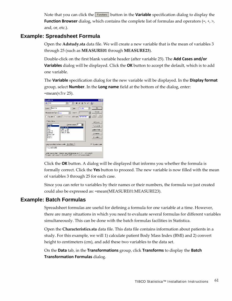
61 TIBCO Statistica™ Installation Instructions
Note that you can click the button in the Variable specification dialog to display the Function Browser dialog, which contains the complete list of formulas and operators (=, +, >, and, or, etc.).
Example: Spreadsheet Formula Open the Adstudy.sta data file. We will create a new variable that is the mean of variables 3 through 25 (such as MEASURE01 through MEASURE23).
Double-click on the first blank variable header (after variable 25). The Add Cases and/or Variables dialog will be displayed. Click the OK button to accept the default, which is to add one variable.
The Variable specification dialog for the new variable will be displayed. In the Display format group, select Number. In the Long name field at the bottom of the dialog, enter: =mean(v3:v 25).
Click the OK button. A dialog will be displayed that informs you whether the formula is formally correct. Click the Yes button to proceed. The new variable is now filled with the mean of variables 3 through 25 for each case.
Since you can refer to variables by their names or their numbers, the formula we just created could also be expressed as: =mean(MEASURE01:MEASURE23).
Example: Batch Formulas Spreadsheet formulas are useful for defining a formula for one variable at a time. However, there are many situations in which you need to evaluate several formulas for different variables simultaneously. This can be done with the batch formulas facilities in Statistica.
Open the Characteristics.sta data file. This data file contains information about patients in a study. For this example, we will 1) calculate patient Body Mass Index (BMI) and 2) convert height to centimeters (cm), and add these two variables to the data set.
On the Data tab, in the Transformations group, click Transforms to display the Batch Transformation Formulas dialog.

62 TIBCO Statistica™ Installation Instructions
The only differences in syntax between the batch transformation formulas and the spreadsheet formulas is the support for multiple formulas in the batch option, and the fact that because the batch formulas are not attached to any specific variable (in fact they can be freely copied from data file to data file), they cannot start with an equal sign, but must have a target variable (for example, v1=... or Measure03=...) so that Statistica knows to which variable each formula should apply.
There is also an option to distribute all batch formulas into the respective variables in the spreadsheet and save them with the data file, effectively replacing the spreadsheet formulas (if there are any).
Following are the calculations used to calculate BMI and to convert Height (in) to centimeters,
Calculation Batch Transformation Dialog Entry
BMI = ('weight (lb)' / 'Height (in)' **2)*703
'Height (cm)' = 'height (in)' *2.54
and the formulas to enter in the Batch Transformation dialog:
In the Formulas field, enter the list of transformation formulas to be applied to the active data spreadsheet. Separate each transformation formula by a return (press ENTER on your keyboard).

63 TIBCO Statistica™ Installation Instructions
Click the OK button in the Batch Transformation Formulas dialog. The Add New Variables? Dialog box will be displayed; click the Yes button to add the two new variables to the Characteristics.sta data file. A message will be displayed to inform you whether the expressions you entered in the Batch Transformation dialog are correct. If they are OK, click Yes to proceed. Statistica calculates the formulas and adds the two variables, BMI and Height (cm), to the spreadsheet.
The options in the Batch Transformation Formulas dialog are particularly well suited (optimized) for transforming large data sets. The formulas will be evaluated one by one, in sequence, so that the results of one transformation in the list can serve as the input for the next. Thus, it is possible to create a new variable with one formula and then use that variable in subsequent formulas.
Click the button in the upper-right corner of the Batch Transformation Formulas dialog to display the Statistica Electronic Manual topic related to these options and links to various other topics containing examples of formulas and syntax rules.
Example 2: Input Data Directly from Excel In addition to using the traditional Statistica spreadsheet, you can open Excel files in a Statistica window and then perform analyses using the Excel file as your data source.
On the Statistica Home tab, in the File group, click the Open arrow and select Open Examples from the drop-down menu to display the Open a Statistica Data File dialog.
From the Files of type drop-down list at the bottom of the dialog, select Excel Files (*.xls;*xlsx;*.xlsm). Double-click the Datasets folder, and then select the Weather report data file, which is an Excel file. Click the Open button, and the Opening file dialog will be displayed.
Click the Open as an Excel Workbook button, and the Excel file will be displayed. Note that when an Excel worksheet is opened in Statistica, the Excel and Statistica menus merge, enabling you to access key functionality for both applications.
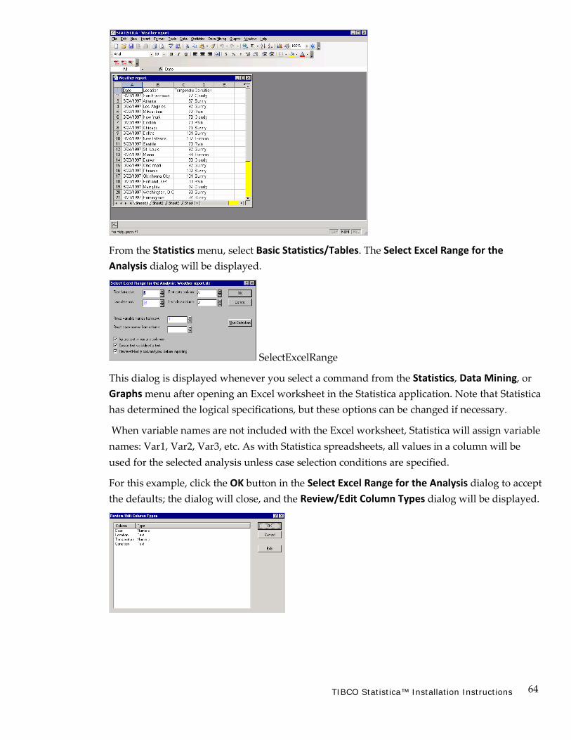
64 TIBCO Statistica™ Installation Instructions
From the Statistics menu, select Basic Statistics/Tables. The Select Excel Range for the Analysis dialog will be displayed.
SelectExcelRange
This dialog is displayed whenever you select a command from the Statistics, Data Mining, or Graphs menu after opening an Excel worksheet in the Statistica application. Note that Statistica has determined the logical specifications, but these options can be changed if necessary.
When variable names are not included with the Excel worksheet, Statistica will assign variable names: Var1, Var2, Var3, etc. As with Statistica spreadsheets, all values in a column will be used for the selected analysis unless case selection conditions are specified.
For this example, click the OK button in the Select Excel Range for the Analysis dialog to accept the defaults; the dialog will close, and the Review/Edit Column Types dialog will be displayed.
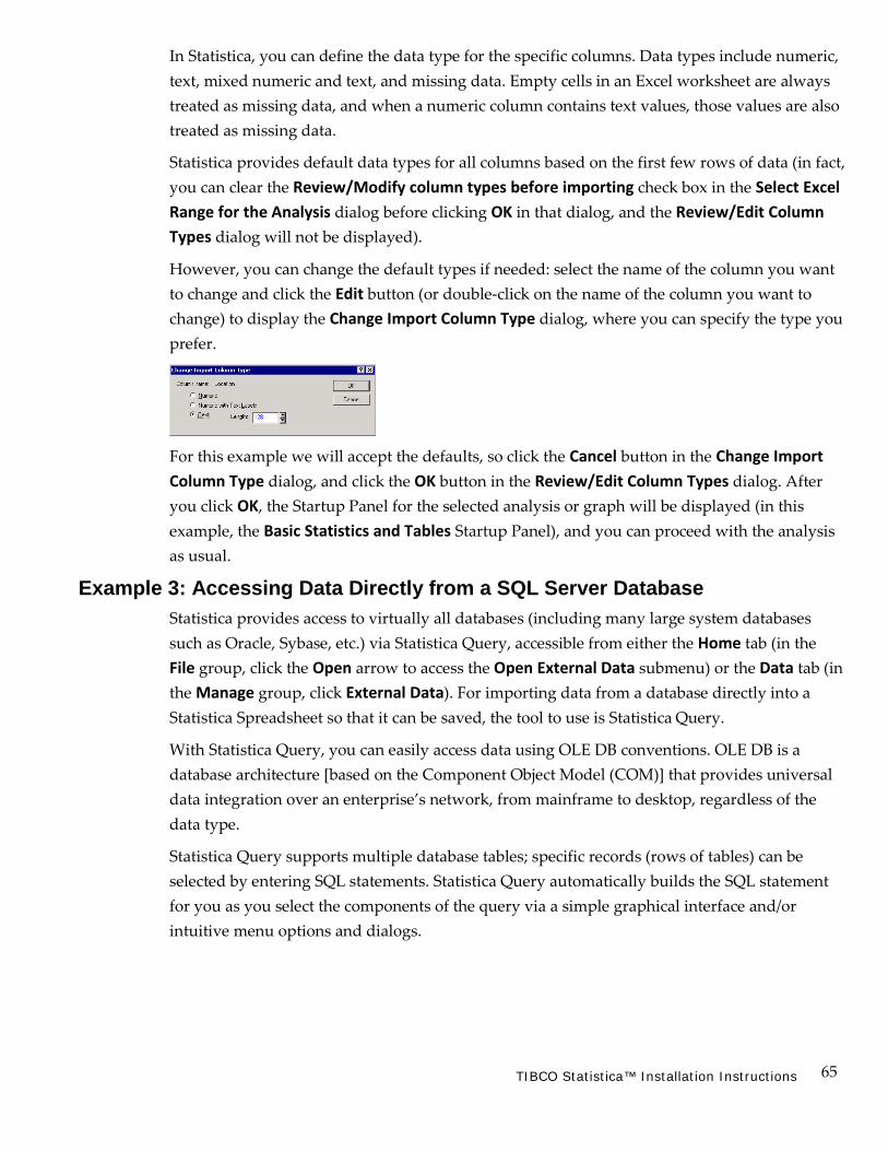
65 TIBCO Statistica™ Installation Instructions
In Statistica, you can define the data type for the specific columns. Data types include numeric, text, mixed numeric and text, and missing data. Empty cells in an Excel worksheet are always treated as missing data, and when a numeric column contains text values, those values are also treated as missing data.
Statistica provides default data types for all columns based on the first few rows of data (in fact, you can clear the Review/Modify column types before importing check box in the Select Excel Range for the Analysis dialog before clicking OK in that dialog, and the Review/Edit Column Types dialog will not be displayed).
However, you can change the default types if needed: select the name of the column you want to change and click the Edit button (or double-click on the name of the column you want to change) to display the Change Import Column Type dialog, where you can specify the type you prefer.
For this example we will accept the defaults, so click the Cancel button in the Change Import Column Type dialog, and click the OK button in the Review/Edit Column Types dialog. After you click OK, the Startup Panel for the selected analysis or graph will be displayed (in this example, the Basic Statistics and Tables Startup Panel), and you can proceed with the analysis as usual.
Example 3: Accessing Data Directly from a SQL Server Database Statistica provides access to virtually all databases (including many large system databases such as Oracle, Sybase, etc.) via Statistica Query, accessible from either the Home tab (in the File group, click the Open arrow to access the Open External Data submenu) or the Data tab (in the Manage group, click External Data). For importing data from a database directly into a Statistica Spreadsheet so that it can be saved, the tool to use is Statistica Query.
With Statistica Query, you can easily access data using OLE DB conventions. OLE DB is a database architecture [based on the Component Object Model (COM)] that provides universal data integration over an enterprise’s network, from mainframe to desktop, regardless of the data type.
Statistica Query supports multiple database tables; specific records (rows of tables) can be selected by entering SQL statements. Statistica Query automatically builds the SQL statement for you as you select the components of the query via a simple graphical interface and/or intuitive menu options and dialogs.
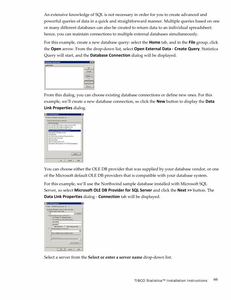
66 TIBCO Statistica™ Installation Instructions
An extensive knowledge of SQL is not necessary in order for you to create advanced and powerful queries of data in a quick and straightforward manner. Multiple queries based on one or many different databases can also be created to return data to an individual spreadsheet; hence, you can maintain connections to multiple external databases simultaneously.
For this example, create a new database query: select the Home tab, and in the File group, click the Open arrow. From the drop-down list, select Open External Data - Create Query. Statistica Query will start, and the Database Connection dialog will be displayed.
From this dialog, you can choose existing database connections or define new ones. For this example, we’ll create a new database connection, so click the New button to display the Data Link Properties dialog.
You can choose either the OLE DB provider that was supplied by your database vendor, or one of the Microsoft default OLE DB providers that is compatible with your database system.
For this example, we’ll use the Northwind sample database installed with Microsoft SQL Server, so select Microsoft OLE DB Provider for SQL Server and click the Next >> button. The Data Link Properties dialog - Connection tab will be displayed.
Select a server from the Select or enter a server name drop-down list.

67 TIBCO Statistica™ Installation Instructions
Then, select the log on option button appropriate to your SQL Server Northwind database installation. Select either the Use Windows NT Integrated security option button, or select the Use a specific user name and password option button and enter a User name and Password in the respective fields.
Next, select Northwind from the Select the database on the server drop-down list.
Click the Test Connection button to attempt a connection to the specified data source. If the connection fails, ensure that the settings are correct. For example, spelling errors and case sensitivity can cause failed connections. If the connection succeeds, click the OK button in the message dialog.
Click OK in the Data Link Properties dialog to display the Add a Database Connection dialog. Enter Northwind in the Name edit box, and click OK.
The Database Connection dialog will be displayed again, with the new Northwind connection defined.
Select this connection, and click OK. The Statistica Query window will be displayed, with all the database tables in the tree view on the left.
Right-click on the Order Details table, and from the shortcut menu, select Add to add the table to the table view pane (the upper-right pane in the Statistica Query window). Then, right-click on the Products table, and add it to the table view pane. Since both tables contain the ProductID field, Statistica Query automatically joins the two tables on this key.

68 TIBCO Statistica™ Installation Instructions
To select the fields to include in the query, right click in the Order Details table in the table view pane, and from the shortcut menu, select Select All Fields. In the Product table, select the ProductName field.
Click the Preview Data tab in the lower-right pane to display a preview of the query.
Click the SQL Statement tab to display the SQL Statement generated by the query.
To return the data to a Statistica Spreadsheet, click the green arrow on the Statistica Query toolbar. The Returning External Data to Spreadsheet dialog will be displayed, where you can control whether the query will be placed into a new or current spreadsheet and adjust other query parameters. Select the New Spreadsheet option button, and click the Run Now button to run the query. If the Connect to OLE DB Provider dialog is displayed, click the OK button. After a few moments, the data is returned to the Statistica Spreadsheet.
Now the data can be analyzed with any of the Statistica tools. Note that the spreadsheet retains the database connection, and you can re-run the query at any time: select the Data tab, and in the Manage group click External Data. Select Refresh Data from the drop-down menu. You can also press F5 on your keyboard when the spreadsheet is open.
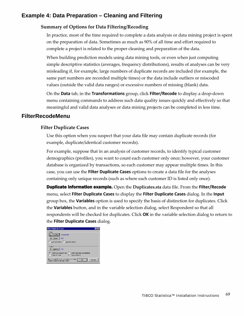
69 TIBCO Statistica™ Installation Instructions
Example 4: Data Preparation – Cleaning and Filtering
Summary of Options for Data Filtering/Recoding
In practice, most of the time required to complete a data analysis or data mining project is spent on the preparation of data. Sometimes as much as 90% of all time and effort required to complete a project is related to the proper cleaning and preparation of the data.
When building prediction models using data mining tools, or even when just computing simple descriptive statistics (averages, frequency distributions), results of analyses can be very misleading if, for example, large numbers of duplicate records are included (for example, the same part numbers are recorded multiple times) or the data include outliers or miscoded values (outside the valid data ranges) or excessive numbers of missing (blank) data.
On the Data tab, in the Transformations group, click Filter/Recode to display a drop-down menu containing commands to address such data quality issues quickly and effectively so that meaningful and valid data analyses or data mining projects can be completed in less time.
FilterRecodeMenu
Filter Duplicate Cases Use this option when you suspect that your data file may contain duplicate records (for example, duplicate/identical customer records).
For example, suppose that in an analysis of customer records, to identify typical customer demographics (profiles), you want to count each customer only once; however, your customer database is organized by transactions, so each customer may appear multiple times. In this case, you can use the Filter Duplicate Cases options to create a data file for the analyses containing only unique records (such as where each customer ID is listed only once).
Duplicate information example. Open the Duplicates.sta data file. From the Filter/Recode menu, select Filter Duplicate Cases to display the Filter Duplicate Cases dialog. In the Input group box, the Variables option is used to specify the basis of distinction for duplicates. Click the Variables button, and in the variable selection dialog, select Respondent so that all respondents will be checked for duplicates. Click OK in the variable selection dialog to return to the Filter Duplicate Cases dialog.

70 TIBCO Statistica™ Installation Instructions
In the Input group box, click the Cases button to display the Spreadsheet Case Selection Conditions dialog, which contains options to select only specified observations or cases for the de-duping operations. In this example, we will filter all the cases, so click the Cancel button in the Spreadsheet Case Selection Conditions dialog.
The Use casenames check box is cleared by default; we will leave this option as is for this example. When this check box is selected, case names are used as one of the bases for distinction, such as Statistica will treat as duplicates any cases that have the same case name (provided the cases match on any other specified variables as well). When the check box is cleared, duplicate case names are ignored.
Clear the Data are sorted check box (because the current data file has not been sorted – when you have an extremely large data file, it is more efficient to sort the data first).
In the Output group box, verify that all variables are selected (ALL will be adjacent to the Variables button). This option is used to select the variables in the input spreadsheet that will be included in the output (filtered) spreadsheet; the default is ALL.
Verify that the Create new spreadsheet check box is selected (the default), and select the Create duplicates spreadsheet check box. Leave the last two options at their defaults: the Preserve order check box is cleared [the new spreadsheets will be sorted by the variable(s) that were selected as the basis of distinction, in this example, Respondent], and the Copy formatting check box is selected. Click OK.
Two new spreadsheets will be generated. One of the spreadsheets is 10v by 51c (10 variables by 51 cases) and contains the respondents from the original spreadsheet excluding the duplications. The other spreadsheet is 10v by 9c and contains the duplicate respondents that were extracted from the original spreadsheet.
Look at the original spreadsheet, Duplicates.sta, and notice that some of the variable headers – Respondent, State, and Colors – are formatted differently. Then look at the two new spreadsheets; the variable headers for Respondent, State, and Colors have the same formatting in all three spreadsheets. Statistica uses sub-setting to create the new spreadsheets and ensures that variable properties of the parent spreadsheet are maintained in the child spreadsheets.
Now, close the two new spreadsheets, but leave the Duplicates.sta spreadsheet open. Notice that it is 10v by 60c. From the Filter/Recode menu, select Filter Duplicate Cases to display the Filter Duplicate Cases dialog again.
In the Input group box, click the Variables button, and in the variable selection dialog, select Respondent and click OK. In the Input group box, clear the Data are sorted check box. In the Output group box, clear the Create new spreadsheet check box. Click OK. The dialog closes and, instead of creating a new spreadsheet with the duplicates excluded, the Duplicates.sta spreadsheet is modified. All duplicate cases are removed from it; it now has 10v by 51c.

71 TIBCO Statistica™ Installation Instructions
Note that the filter duplicate cases functionality does not use case sensitivity (upper-case, lower-case letters) for a comparison of uniqueness, such as if you have two respondents – C. Barrett and C. BARRETT – the second respondent will be excluded.
Filter Sparse Data It is not uncommon that some variables (parameters, or data fields) available for (for example) predictive modeling have very few valid data. For example, in a customer database self- reported (by customers) Income may be recorded; however, very few customers actually volunteered their current incomes, so most of the data (in that field of the database) is blank (or missing). In manufacturing data, a data field may exist to record a specific parameter, but the sensor might be faulty for an extended period of time, recording mostly missing (invalid) data.
Including such sparsely populated (with data) variables in an analysis may lead to erroneous results, or prevent you from building predictive models altogether (depending on how the missing data are handled later in the analyses). Therefore, you may want to identify such sparse variables ahead of time using the Filter Sparse Data options (accessible from the Filter/Recode menu located on the Data tab in the Transformations group), and eliminate them from subsequent consideration.
Process Invariant Variables A similar (to the sparse-data case) data quality issue that often occurs, in particular in industrial manufacturing (process) data, is that some variables (parameters) that are recorded and included in the analyses are invariant, such as all values are the same.

72 TIBCO Statistica™ Installation Instructions
Such variables are not useful for predictive modeling, and the Process Invariant Variables options (accessible from the Filter/Recode menu located on the Data tab in the Transformations group) enable you to identify those variables automatically, and exclude them from further analyses.
Recode Outliers Extreme data values or outliers can greatly affect various analyses and cause poor accuracy of prediction (data mining) models. There is no formal definition of what constitutes an outlier or extreme value, and Statistica’s graphical tools may provide the best way to review data to identify such unusual observations (for example, you could create box plots of the key variables to identify extreme observations and brush or flag them in the data).
To automatically process lists of variables to identify and remove outliers, the Recode Outliers options (accessible from the Filter/Recode menu located on the Data tab in the Transformations group) provide several tests for outliers (approaches for identifying extreme values).
Outliers can be recoded to missing data or to valid data values (for example, to the respective percentile boundary values, etc.).

73 TIBCO Statistica™ Installation Instructions
Process Missing Data Missing data or invalid data values must obviously be dealt with in a manner that is consistent with the goals of the analyses. In some cases, missing or invalid data may themselves provide useful information about a process or variable of interest. For example, in marketing research, it is common that respondents will refuse to provide detailed personal information regarding their health, financial status (for example, savings), etc., and such refusal itself may be correlated with other significant variables of interest (for example, refusal to answer questions related to income may itself be a good indicator of high income, if indeed wealthier individuals in the survey tended not to answer those questions).
The Process Missing Data options (accessible from the Filter/Recode menu located on the Data tab in the Transformations group) enable you to recode missing data flexibly, define multiple missing data values or codes for a single variable (which can then be recoded to the variable missing data code), or just to flag variables that have more than a certain percentage of missing data.
Imputation of Missing Data (k-Nearest Neighbor) It is often not clear how best to recode missing data, and in fact, sometimes by recoding missing data for a particular variable to a specific value (for example, the mean), the final results may be biased.
For example, suppose in a survey all respondents who refuse to report their income tend to be in the higher income bracket. In that case, assigning the mean-income to those individuals (such as recoding missing data for variable Income to the mean income for the whole sample) may yield highly misleading results.
Statistica includes a very efficient method (applicable to very large data sets and databases) for replacing missing data with valid data values that are consistent with the other observations in the sample.

74 TIBCO Statistica™ Installation Instructions
In short, using the MD Imputation options (accessible from the Filter/Recode menu), in a first pass through the data, the k-nearest neighbor algorithm will select a (smaller) sample from all available data. In the second pass through the data file, when missing data are encountered, they are replaced with valid (observed) values found in similar observations in the smaller sample (with respect to all other variables that were selected). So to continue this example, if indeed higher-income respondents are less likely to report this fact, but do report other indicators of high-income (for example, ownership of a luxury car, more square footage of their home, etc.), then the k-nearest neighbor algorithm will accurately assign those individuals (who failed to report their income) to the high-income bracket.
The k-nearest neighbor algorithm is fast and efficient, and provides an effective method for replacing missing data in the input file with “reasonable guesses” based on similar data points in the sample. This approach does not make any particular assumptions about the nature of the relationships between variables (such as require that a model be estimated for each variable to predict missing data values), but simply uses the observed data as the model.
Merge Data Files The Statistica Merge Options dialog enables you to merge two data files either by the variables or by the cases so that you can centralize all of the observations to one table. Select the Data tab, and in the Manage group, click Merge to display the Merge Options dialog.
Click the Help button in the upper-right corner of the dialog to access Help topics describing all the options in this dialog.

75 TIBCO Statistica™ Installation Instructions
Creating Subsets If you have a large spreadsheet, you may want to create a new spreadsheet containing a specified subset of the current spreadsheet. For example, open Boston2.sta. This data set contains over a thousand cases. We want to extract housing tracts with low median prices.
Select the Data tab, and in the Manage group, click Subset to display the Create a Subset dialog.
Click the Cases button to display the Spreadsheet Case Selection Conditions dialog, which contains options to create conditions to define the selection of cases to be considered for the sample.
Select the Enable Selection Conditions check box to activate the options, and then select the Specific, selected by option button in the Include cases group box to specify which cases to include in the analysis. Type v1=‘LOW’ in the Expression text box.
Click the OK button to set the selection conditions and return to the Create a Subset dialog, and click the OK button in this dialog to create the new spreadsheet.
The resultant spreadsheet contains 334 cases (instead of the original 1,012 cases) and all 15 variables from the original spreadsheet. For the PRICE variable, all cases have a value of LOW.
Example 5: Using Statistica ETL (Extract, Transform, and Load) The Statistica ETL (Extract, Transform, and Load) module provides unique capabilities for processing and merging data, in particular, process data that are difficult to manage using standard database tools. ETL automates the process of validating and aligning multiple diverse data sources into a single source suitable for ad-hoc or automated analyses.

76 TIBCO Statistica™ Installation Instructions
ETL offers two options for aligning data: Time-indexed, which aggregates data from multiple data sources based on a date/time stamp variable and aligns data by minute, hour, day, week, month, quarter, or year; and ID-based, which aggregates data from multiple data sources based on an identifier variable and an optional time variable, and optionally aligns data by N equal intervals or N user-specified intervals.
This example illustrates how the ETL module handles stock-related data sets with different time intervals. Stocks are bought and sold at varying prices throughout each day. Microsoft (ticker MSFT) and Oracle (ticker ORCL) are software companies that trade on the NASDAQ electronic stock exchange. In this example, we will compare data sets containing historical stock prices with different date/time stamps. The first set contains daily Microsoft price quotes from NASDAQ, while the second set contains weekly Oracle price quotes from another source.
Open MicrosoftPrices.sta and OraclePrices.sta: on the Home tab in the File group, click the Open arrow. From the drop-down menu, select Open Examples to display the Open a Statistica Data File dialog. Double-click on the Datasets folder, select MicrosoftPrices.sta and OraclePrices.sta, and click the Open button.
Both data files contain the following columns (variables): DATE - the day on which a trade takes place; OPEN - opening price for the day, first trade of the day; HIGH - the highest price of the day; LOW - the lowest price of the day; CLOSE - closing price for the day, last trade of the day; and VOLUME - the daily number of traded shares of a security.
However, they have different date ranges: Microsoft - 10/22/2007-01/04/2008; Oracle - 10/18/2007-12/28/2007. In order to compare the data, the ranges will need to be aligned.
Select the Data tab. In the Manage group, click External Data, and select Time-indexed Process Data from the Extract, Transform, and Load (ETL) submenu. The Statistica Extract, Transform, and Load (ETL): Time-indexed Startup Panel is displayed.
Click the Add data source button to display the Select Data Sources dialog.

77 TIBCO Statistica™ Installation Instructions
Click the Documents button to display the Select Documents dialog. Select the Open Spreadsheets Documents check box to select both data files (MicrosoftPrices.sta and OraclePrices.sta).
Click the OK button in the Select Documents dialog, and then click the OK button in the Select Data Sources dialog. The Statistica Extract, Transform, and Load (ETL): Time-indexed Startup Panel will appear as shown below:
Select MicrosoftPrices.sta in the file list at the top of the dialog, and click the Variables button to display the Select variables dialog. Select DATE from the Date/Time stamp list, and select CLOSE from the Variables list.
Click the OK button to close this dialog and return to the Statistica Extract, Transform, and Load (ETL): Time-indexed Startup Panel.
Now select OraclePrices.sta in the file list. Click the Variables button, and select variable 1 from the Date/Time stamp list and variable 5 from the Variables list, and then click the OK button.
In the Aggregation interval for all data source(s) group box, select the Weekly option button, and change the start from field to Friday.

78 TIBCO Statistica™ Installation Instructions
For additional date/time options, select the Options tab. Select the Filter all input data sources by the following Date/Time check box. To limit the data that is returned from both of the selected data files, enter 11/2/2007 in the Start date field and 12/28/2007 in the End date field. This will return eight weeks of data (Friday to Friday).
Now, click the Results button to merge the data into a spreadsheet.
The two data files are now aligned weekly by date for the range 11/2/2007 to 12/28/2007. The daily closing Microsoft prices are aggregated as means, while the weekly closing Oracle prices are unchanged.
The Results spreadsheet displays date/time stamps as cases names so that they can be used for graphing the aggregated and aligned data.
Select the Graphs tab. In the More group, click 2D and select Line Plots (Variables) to display the 2D Line Plots - Variables dialog.

79 TIBCO Statistica™ Installation Instructions
Click the Variables button, and in the variable selection dialog, select variables 2 and 3. Then, click the OK button. In the 2D Lineplots - Variables dialog, select Multiple for the Graph type, and click the OK button. The following image shows the resultant graph plotting Microsoft and Oracle prices.
Enterprise Installations Example 1: Statistica Enterprise Server – Download/Offload Analyses from/to Servers
Statistica Enterprise Server extends the capabilities of the Statistica platform, turning several standalone workstations into a powerful, enterprise-wide collaborative-intelligence system.
One of the key features of Statistica Enterprise Server’s client-server architecture is that it enables you to utilize server-side resources to run multiple, possibly time-consuming, or repetitive statistical analyses (offload tasks to the server) while at the same time freeing the local system for other tasks that require immediate attention.
This can be achieved using either a Web browser (thin client) or desktop version of Statistica (thick client, Statistica Enterprise Server client).
While the former allows access to Statistica Enterprise Server using only a browser, the latter requires Statistica installation on your computer. Statistica Enterprise Server’s tight integration with the Statistica application provides common user experience and workflow for both client and server-side operations, a generally more feature-rich and responsive user interface, and all the additional components and tools of desktop Statistica.
Offloading an analysis (or a custom script) to Statistica Enterprise Server. First, ensure that Statistica Enterprise Server integration is enabled. Select the Home tab, and in the Tools group click Options to display the Options dialog. In the tree view, select Server/Web.

80 TIBCO Statistica™ Installation Instructions
Select the Enable Statistica Enterprise Server Integration check box. The only required parameter is Statistica Enterprise Server’s network path (and connection settings, if they are different from the default). Ask your network administrator for these values. It is possible to Enable Integrated Login if it is supported and enabled on the server; otherwise you will need to enter your user name and password when logging in to Statistica Enterprise Server.
After specifying the options on this tab, click the OK button.
The Server tab has now been added to the ribbon bar. In the User group, click Log In, and enter your user name and password if requested. Upon successfully establishing a connection, the options on the Server tab will become available.
The Open, Save, and Save As commands in the File group are used to upload a currently open file to the server or download a file and open it locally. There are also explicit options in the Transfer group to Download File to and Upload File from specific folders on the server and the client.
Note: As real-world examples of time- or resource-consuming analyses are usually based on large data sets and/or involve iterative algorithms represented by Statistica components that are not included in all configurations of Statistica, we are deliberately going to use an example that does not require much time to complete.
But even in a situation where a single analysis is quick and not resource-intensive, you might need to run a fairly complicated, time-consuming sequence of tasks, possibly scheduled at certain time intervals.
In this case, the Statistica Enterprise Server scheduling facilities could be used once you have created and uploaded a custom script that represents the required tasks (for example, by combining the macros recorded during a Statistica session).
Now, record a sample analysis macro; for example, complete the steps described in Example 2: ANOVA.

81 TIBCO Statistica™ Installation Instructions
After completing the example, in the ANOVA Results dialog, click the Options button (located at the bottom of the dialog), and from the drop-down list, select Create Macro. In the New Macro dialog, accept all defaults, and click OK. Test the generated macro by running it (press F5) to ensure that it produces results as expected. Click on the macro code window to ensure it has the focus.
Then, on the Server tab in the Tasks group, click Offload to display the Offload a task dialog.
We need to select a task to offload (a script or a Data Miner project) and, optionally, a data set on which the task will operate (the data set could be an optional component since Data Miner projects may have their data sets embedded and macros might explicitly load data sets or not require them at all).
Since there is an open active data set (Adstudy.sta) and an open Statistica Macro (our sample analysis), the default settings of the options in the Offload a task dialog specify to use them for offloading.
Instead, this example will demonstrate how to reference a task and a server-side data set. This option is useful since it gives you the advantage of central server-side storage, which is especially beneficial in the case of large data sets (possibly dynamically updated) that are used by multiple users.
To reference a server-side data set, in the Data Source group box, select the Select data file stored on the server option button to display the Statistica Enterprise Server Repository dialog.
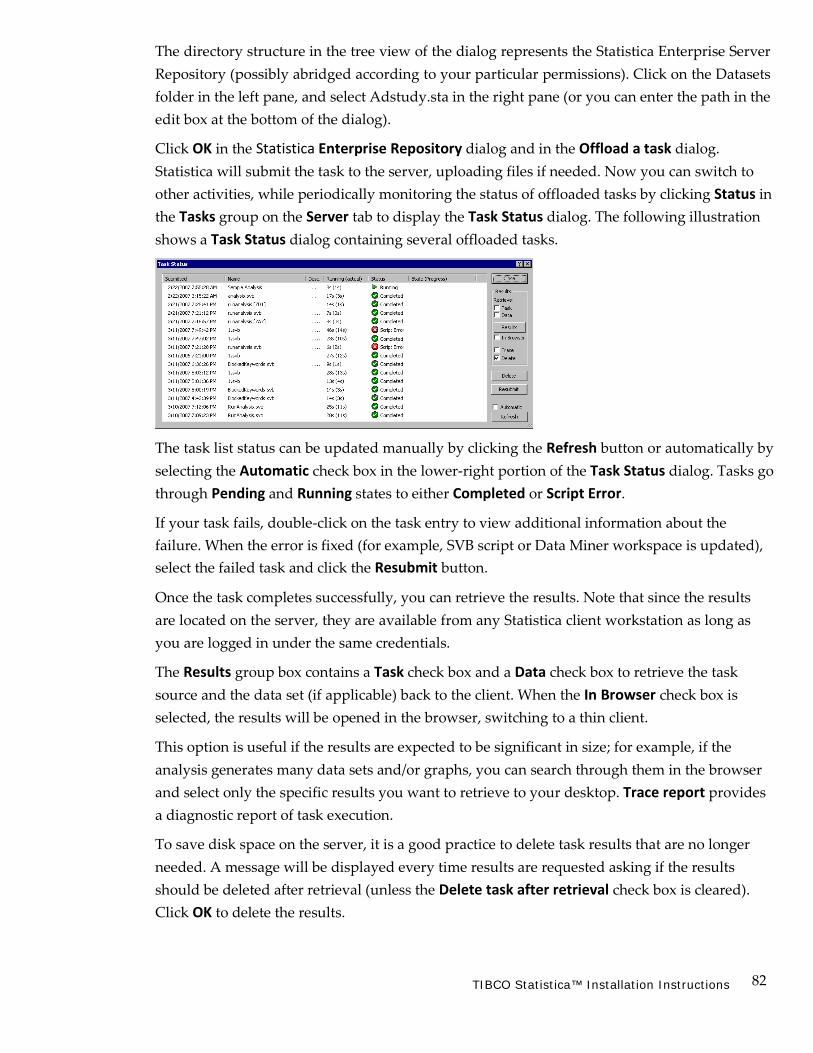
82 TIBCO Statistica™ Installation Instructions
The directory structure in the tree view of the dialog represents the Statistica Enterprise Server Repository (possibly abridged according to your particular permissions). Click on the Datasets folder in the left pane, and select Adstudy.sta in the right pane (or you can enter the path in the edit box at the bottom of the dialog).
Click OK in the Statistica Enterprise Repository dialog and in the Offload a task dialog. Statistica will submit the task to the server, uploading files if needed. Now you can switch to other activities, while periodically monitoring the status of offloaded tasks by clicking Status in the Tasks group on the Server tab to display the Task Status dialog. The following illustration shows a Task Status dialog containing several offloaded tasks.
The task list status can be updated manually by clicking the Refresh button or automatically by selecting the Automatic check box in the lower-right portion of the Task Status dialog. Tasks go through Pending and Running states to either Completed or Script Error.
If your task fails, double-click on the task entry to view additional information about the failure. When the error is fixed (for example, SVB script or Data Miner workspace is updated), select the failed task and click the Resubmit button.
Once the task completes successfully, you can retrieve the results. Note that since the results are located on the server, they are available from any Statistica client workstation as long as you are logged in under the same credentials.
The Results group box contains a Task check box and a Data check box to retrieve the task source and the data set (if applicable) back to the client. When the In Browser check box is selected, the results will be opened in the browser, switching to a thin client.
This option is useful if the results are expected to be significant in size; for example, if the analysis generates many data sets and/or graphs, you can search through them in the browser and select only the specific results you want to retrieve to your desktop. Trace report provides a diagnostic report of task execution.
To save disk space on the server, it is a good practice to delete task results that are no longer needed. A message will be displayed every time results are requested asking if the results should be deleted after retrieval (unless the Delete task after retrieval check box is cleared). Click OK to delete the results.

83 TIBCO Statistica™ Installation Instructions
Once our task completes, we retrieve the results and close the Task Status dialog. Results are equivalent whether run locally or on the server.
Example 2: Using Statistica in Regulated Environments In a regulated environment, analyses conducted for GxP (Good Manufacturing Practices, Good Clinical Practices, Good Laboratory Practices) applications are ones that impact consumer safety such as in clinical trials, manufacturing, and quality control.
When a business conducts analyses for a GxP application, regulatory bodies recommend that the company be able to prove that the results of the validated analysis system (for example, Statistica) are under control. Statistica, through its audit trail and spreadsheet/report locking features, offers the tools you need to meet this regulatory requirement.
In order to meet traceability requirements for GxP applications, there are at least three concerns: 1) control of the input data being submitted to the analysis (such as knowing who made what change, at what time, for what reason; and the old values and new values), 2) control of the results tables and graphs (for example, demonstrate that they were not altered in any way after they were created), and 3) traceability between the version of the input spreadsheet and the results outputs. Statistica provides this information through its Spreadsheet Audit Trails and GxP Reports functionality.
Control of Input Data Enable Audit Trail Logging
Open a Statistica Spreadsheet. Select the Tools tab, click Audit Trail, and select Settings from the drop-down menu. The Spreadsheet Audit Log Settings dialog will be displayed. Select the Enable audit trail logging check box to enable audit trail logging for the current spreadsheet.
When spreadsheet audit trail logging is enabled, the spreadsheet is automatically set to direct mode, such as changes made to the spreadsheet will be immediately written to disk. Thus, when audit trail logging is enabled, changes to the data file cannot be undone.

84 TIBCO Statistica™ Installation Instructions
Select the Require users to enter reason comments for each change check box to require users to explain each change made to the spreadsheet.
The Truncate log button is available only if audit trail logging has previously been specified, and there is a current Spreadsheet Audit Log Viewer attached to the spreadsheet.
Clicking this button will truncate the spreadsheet log and delete all existing entries. You will be prompted to confirm this action before the current entries are deleted. Once the log is truncated, the truncate action will be recorded in the newly truncated log file.
Click OK in the Spreadsheet Audit Log Settings dialog, and audit trail logging will be enabled; in fact, the Enter reason for change dialog will be displayed immediately in order to enter the reason for enabling the logging function. Enter a comment, and click OK.
Now, right-click in the header of the last variable in the spreadsheet, and select Add Variables from the shortcut menu. In the Add Variables dialog, we will accept all defaults, so click OK. The Enter reason for change dialog will be displayed; you must enter a comment and click OK before the change will be made. When audit trail logging is enabled, every change made to the spreadsheet will be documented, and when the Require users to enter reason comments for each change check box is selected, user comments also will be stored and displayed in the Spreadsheet Audit Log Viewer.
Next, on the Tools tab, click Audit Trail and select View Log to display the Spreadsheet Audit Log Viewer.
The log viewer displays a grid of information regarding the audited actions including the sequence number, time of change, the computer used to make the change, user information, the nature of the change, and the reason for the change. Column widths in the log grid can be increased and decreased using standard Windows techniques. The Spreadsheet Audit Trails are saved and embedded into each respective spreadsheet.
Password encryption vs. locking. A spreadsheet can be password encrypted so that it cannot be opened without the correct password. Only users who know the password can open the spreadsheet. Once a password encrypted spreadsheet is opened, it can be modified.
Alternatively, locking a spreadsheet makes portions of the spreadsheet read-only, enabling you to prevent changes to some or all aspects of the spreadsheet. The spreadsheet can be opened by anyone, but locked portions cannot be altered.
Both the password encryption options and spreadsheet locking facilities can be used simultaneously.
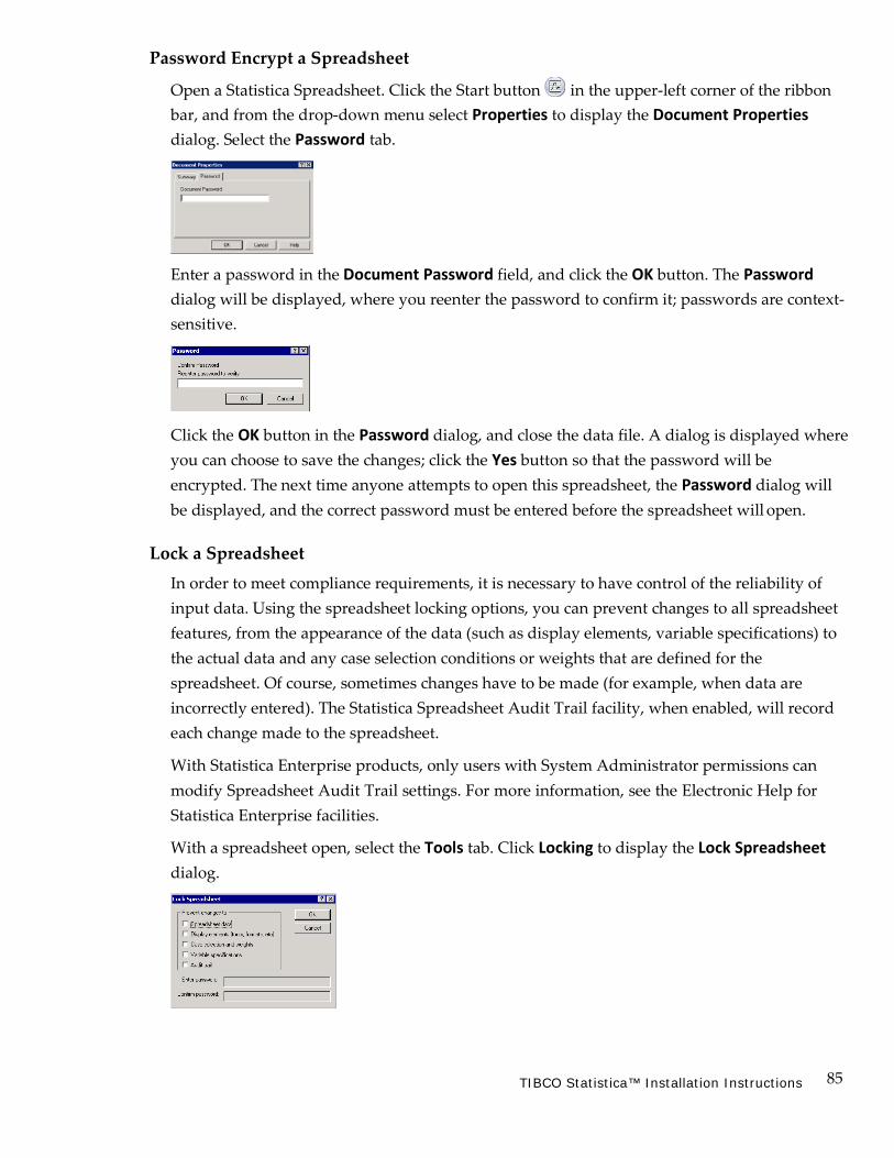
85 TIBCO Statistica™ Installation Instructions
Password Encrypt a Spreadsheet
Open a Statistica Spreadsheet. Click the Start button in the upper-left corner of the ribbon bar, and from the drop-down menu select Properties to display the Document Properties dialog. Select the Password tab.
Enter a password in the Document Password field, and click the OK button. The Password dialog will be displayed, where you reenter the password to confirm it; passwords are context- sensitive.
Click the OK button in the Password dialog, and close the data file. A dialog is displayed where you can choose to save the changes; click the Yes button so that the password will be encrypted. The next time anyone attempts to open this spreadsheet, the Password dialog will be displayed, and the correct password must be entered before the spreadsheet will open.
Lock a Spreadsheet In order to meet compliance requirements, it is necessary to have control of the reliability of input data. Using the spreadsheet locking options, you can prevent changes to all spreadsheet features, from the appearance of the data (such as display elements, variable specifications) to the actual data and any case selection conditions or weights that are defined for the spreadsheet. Of course, sometimes changes have to be made (for example, when data are incorrectly entered). The Statistica Spreadsheet Audit Trail facility, when enabled, will record each change made to the spreadsheet.
With Statistica Enterprise products, only users with System Administrator permissions can modify Spreadsheet Audit Trail settings. For more information, see the Electronic Help for Statistica Enterprise facilities.
With a spreadsheet open, select the Tools tab. Click Locking to display the Lock Spreadsheet dialog.
86 TIBCO Statistica™ Installation Instructions
Here, you can specify which aspects of the spreadsheet that you want to lock. When users try to change a locked feature, a message will be displayed, informing them that the spreadsheet is locked.
Select the Spreadsheet data check box to prevent changes to the actual data contained in the spreadsheet. Users will be unable to change the data values and the missing data code.
They will also be unable to perform any data management operations that affect the spreadsheet (for example, change the data type or the length for text variables). If this check box is cleared, users will be able to edit the data (for example, by updating queries and Spreadsheet Formulas or by simply typing in new values).
Select the Display elements (fonts, formats, etc.) check box to prohibit the modification of fonts and formats used in the spreadsheet. Options for changing the font size, color, type, and style (such as bold, underline) will be dimmed. Additionally, the options for applying spreadsheet layouts (accessible by selecting the Format tab and clicking Layouts in the Spreadsheet group) will be unavailable.
Select the Case selection and weights check box to prevent users from changing case selection conditions and case weights for the locked spreadsheet. Users will not be able to toggle the use of selection conditions or change the currently defined selection conditions.
Most options on the Selection tab of the Spreadsheet Case Selection Conditions dialog will be dimmed; however, options on the other tabs of that dialog (for example, creating subsamples, applying formats to selection conditions) are still available. Options on the Case Weights dialog will be unavailable.
Select the Variable specifications check box to prevent changes to the variable specifications (for example, measurement type, missing data code, display format, long variable name). Users will still be able to view the individual variable specification dialog (accessible by double- clicking the variable header) and the Variable Specifications Editor; however, options for changing these specifications will be dimmed.
Select the Audit trail check box to prevent changes to the audit trail settings. Users will be unable to modify the audit trail settings.
Enter a password to use when locking and unlocking the spreadsheet, confirm the password (which is context sensitive), and click OK. Although a password is not required, it is strongly recommended. If a password is not entered and confirmed, any user can unlock spreadsheet features by simply clearing the selected check boxes. Note that if locks have already been defined, you must enter the correct password before locks can be changed or modified.
Now try making changes in the spreadsheet; a message will be displayed informing you that the operation cannot be completed because the spreadsheet is locked.
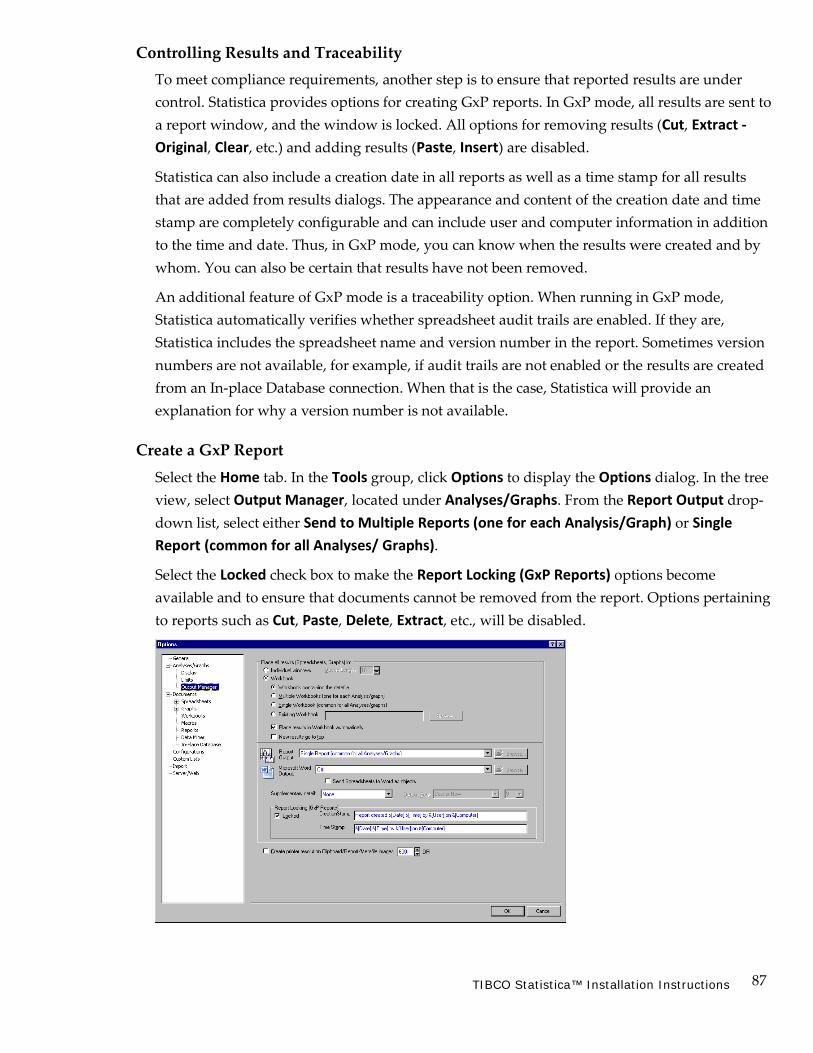
87 TIBCO Statistica™ Installation Instructions
Controlling Results and Traceability To meet compliance requirements, another step is to ensure that reported results are under control. Statistica provides options for creating GxP reports. In GxP mode, all results are sent to a report window, and the window is locked. All options for removing results (Cut, Extract - Original, Clear, etc.) and adding results (Paste, Insert) are disabled.
Statistica can also include a creation date in all reports as well as a time stamp for all results that are added from results dialogs. The appearance and content of the creation date and time stamp are completely configurable and can include user and computer information in addition to the time and date. Thus, in GxP mode, you can know when the results were created and by whom. You can also be certain that results have not been removed.
An additional feature of GxP mode is a traceability option. When running in GxP mode, Statistica automatically verifies whether spreadsheet audit trails are enabled. If they are, Statistica includes the spreadsheet name and version number in the report. Sometimes version numbers are not available, for example, if audit trails are not enabled or the results are created from an In-place Database connection. When that is the case, Statistica will provide an explanation for why a version number is not available.
Create a GxP Report Select the Home tab. In the Tools group, click Options to display the Options dialog. In the tree view, select Output Manager, located under Analyses/Graphs. From the Report Output drop- down list, select either Send to Multiple Reports (one for each Analysis/Graph) or Single Report (common for all Analyses/ Graphs).
Select the Locked check box to make the Report Locking (GxP Reports) options become available and to ensure that documents cannot be removed from the report. Options pertaining to reports such as Cut, Paste, Delete, Extract, etc., will be disabled.

88 TIBCO Statistica™ Installation Instructions
To include a creation stamp at the top of the file, you can accept the default format in the CreationStamp field, or enter your own. The following codes can be used in this field: &[Date], &[Time], &[User], and &[Computer]. Any text you enter will be displayed as is.
To include a time stamp above each object as it is added to the report, you can accept the default format in the Time Stamp field, or enter your own. The following codes can be used in this field: &[Date], &[Time], &[User], and &[Computer].
Click OK in the Options dialog, and now perform any analysis; for example, use Basic Statistics to create a quick Descriptive Statistics summary spreadsheet. When you click the Summary button, the results will be sent to a locked report that lists the creator, date, time, etc., of the analysis.
Example 3: Statistica Enterprise Statistica Enterprise products extend the functionality of Statistica applications by offering collaborative work, central administration, system level customization, and other features necessary when using Statistica applications as part of the enterprise-level computer systems.
Statistica Enterprise Manager is a component of the Statistica Enterprise system that enables users to configure various aspects of the Enterprise system including user administration, system view organization, database connection maintenance, data configurations, and analysis configurations.
For this example, we will:
1. Create a new user
2. Create a new group
a. Assign permissions to the group b.Add the user (see No. 1) to the group
3. Create a system view node
4. Create a new database connection
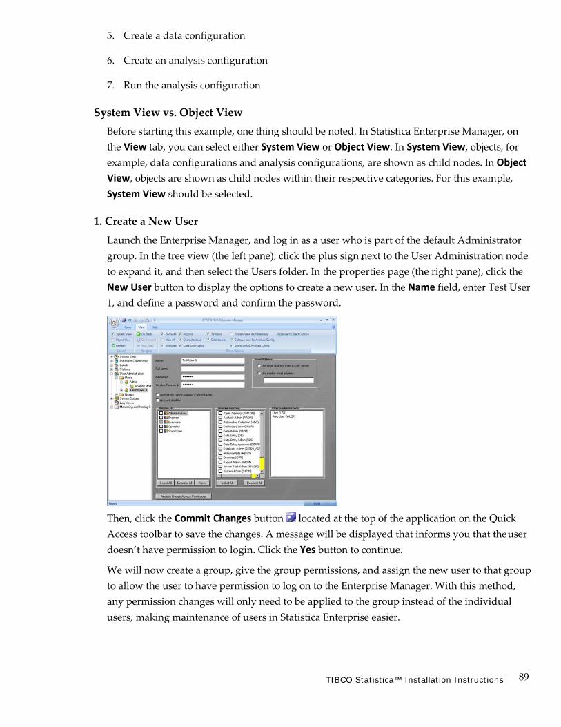
89 TIBCO Statistica™ Installation Instructions
5. Create a data configuration
6. Create an analysis configuration
7. Run the analysis configuration
System View vs. Object View Before starting this example, one thing should be noted. In Statistica Enterprise Manager, on the View tab, you can select either System View or Object View. In System View, objects, for example, data configurations and analysis configurations, are shown as child nodes. In Object View, objects are shown as child nodes within their respective categories. For this example, System View should be selected.
1. Create a New User Launch the Enterprise Manager, and log in as a user who is part of the default Administrator group. In the tree view (the left pane), click the plus sign next to the User Administration node to expand it, and then select the Users folder. In the properties page (the right pane), click the New User button to display the options to create a new user. In the Name field, enter Test User 1, and define a password and confirm the password.
Then, click the Commit Changes button located at the top of the application on the Quick Access toolbar to save the changes. A message will be displayed that informs you that the user doesn’t have permission to login. Click the Yes button to continue.
We will now create a group, give the group permissions, and assign the new user to that group to allow the user to have permission to log on to the Enterprise Manager. With this method, any permission changes will only need to be applied to the group instead of the individual users, making maintenance of users in Statistica Enterprise easier.

90 TIBCO Statistica™ Installation Instructions
2. Create a New Group In the User Administration node, select the Groups folder, and in the properties page, click the New Group button to display the options to create a new group. In the Name field, enter Test Group 1. In the Group Members frame, select the check box adjacent to Test User 1.
This will add the previously created user to the group. In the Group Permissions frame, select the check boxes adjacent to Analysis Admin (AADM) and Web User (WUSR). In the tree view, click the plus sign adjacent to the Test Group 1 node to expand it, and select Analysis modules. In the properties page, click the Select All button to select all of the modules in the Available analysis module(s) list.
This will give users of this group permission to log on to both Web and desktop Statistica and run all of the available analyses and reports.
Click the Commit Changes button to save the changes.
We have now created the necessary user and group security to run analyses and reports. When creating the data, analysis, and report configurations in the next steps, we will assign this group to those objects to allow only users within the group to run them.
3. Create a System View Node Now we will create a System View node to hold this example’s data, analyses, and report configuration. In the tree view, click the plus sign adjacent to the System View node to expand it. Right-click on the Statistica Enterprise folder, and from the shortcut menu, select New Folder. In the Folder name text box in the properties page, enter Test Example 1 as the new folder’s name.
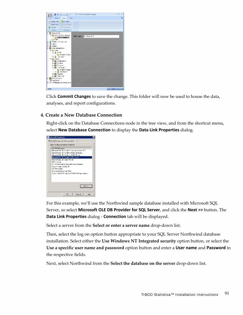
91 TIBCO Statistica™ Installation Instructions
Click Commit Changes to save the change. This folder will now be used to house the data, analyses, and report configurations.
4. Create a New Database Connection Right-click on the Database Connections node in the tree view, and from the shortcut menu, select New Database Connection to display the Data Link Properties dialog.
For this example, we’ll use the Northwind sample database installed with Microsoft SQL Server, so select Microsoft OLE DB Provider for SQL Server, and click the Next >> button. The Data Link Properties dialog - Connection tab will be displayed.
Select a server from the Select or enter a server name drop-down list.
Then, select the log on option button appropriate to your SQL Server Northwind database installation. Select either the Use Windows NT Integrated security option button, or select the Use a specific user name and password option button and enter a User name and Password in the respective fields.
Next, select Northwind from the Select the database on the server drop-down list.
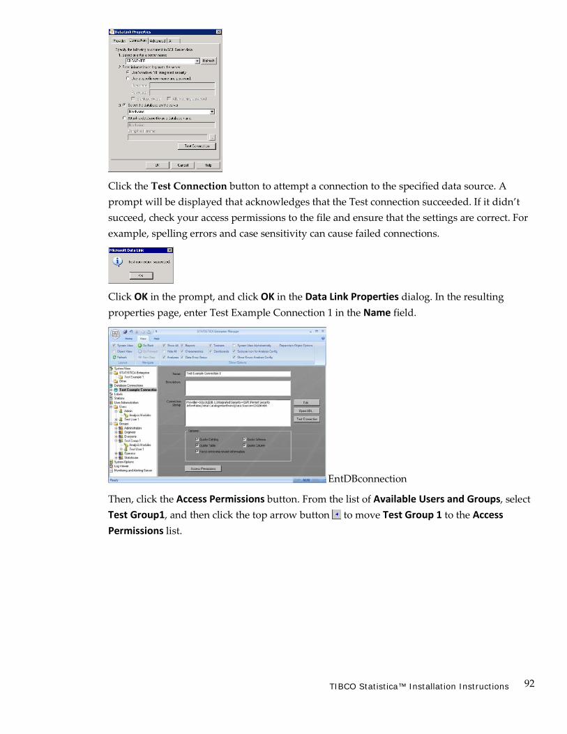
92 TIBCO Statistica™ Installation Instructions
Click the Test Connection button to attempt a connection to the specified data source. A prompt will be displayed that acknowledges that the Test connection succeeded. If it didn’t succeed, check your access permissions to the file and ensure that the settings are correct. For example, spelling errors and case sensitivity can cause failed connections.
Click OK in the prompt, and click OK in the Data Link Properties dialog. In the resulting properties page, enter Test Example Connection 1 in the Name field.
EntDBconnection
Then, click the Access Permissions button. From the list of Available Users and Groups, select Test Group1, and then click the top arrow button to move Test Group 1 to the Access Permissions list.
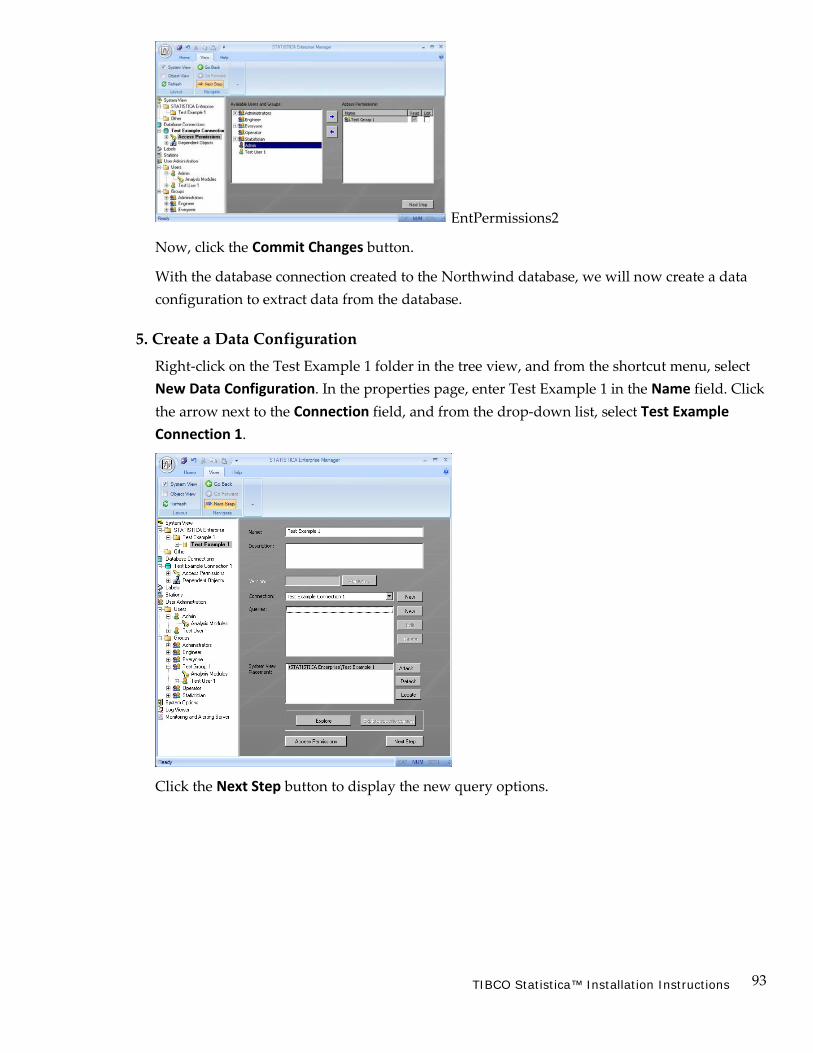
93 TIBCO Statistica™ Installation Instructions
EntPermissions2
Now, click the Commit Changes button.
With the database connection created to the Northwind database, we will now create a data configuration to extract data from the database.
5. Create a Data Configuration Right-click on the Test Example 1 folder in the tree view, and from the shortcut menu, select New Data Configuration. In the properties page, enter Test Example 1 in the Name field. Click the arrow next to the Connection field, and from the drop-down list, select Test Example Connection 1.
Click the Next Step button to display the new query options.

94 TIBCO Statistica™ Installation Instructions
Click the SQL Wizard button to display the New Query dialog, which will open in Statistica.
Drag the Orders table from the left pane into the editor viewer (the upper-right pane), and then select, in the following order, the OrderID, Ship Via, ShipCountry, and Freight fields.
Select the Preview Data tab in the query properties view (lower-right pane) and click the Refresh toolbar button (the red exclamation mark). This will test the query to ensure that values are being retrieved from the defined query.
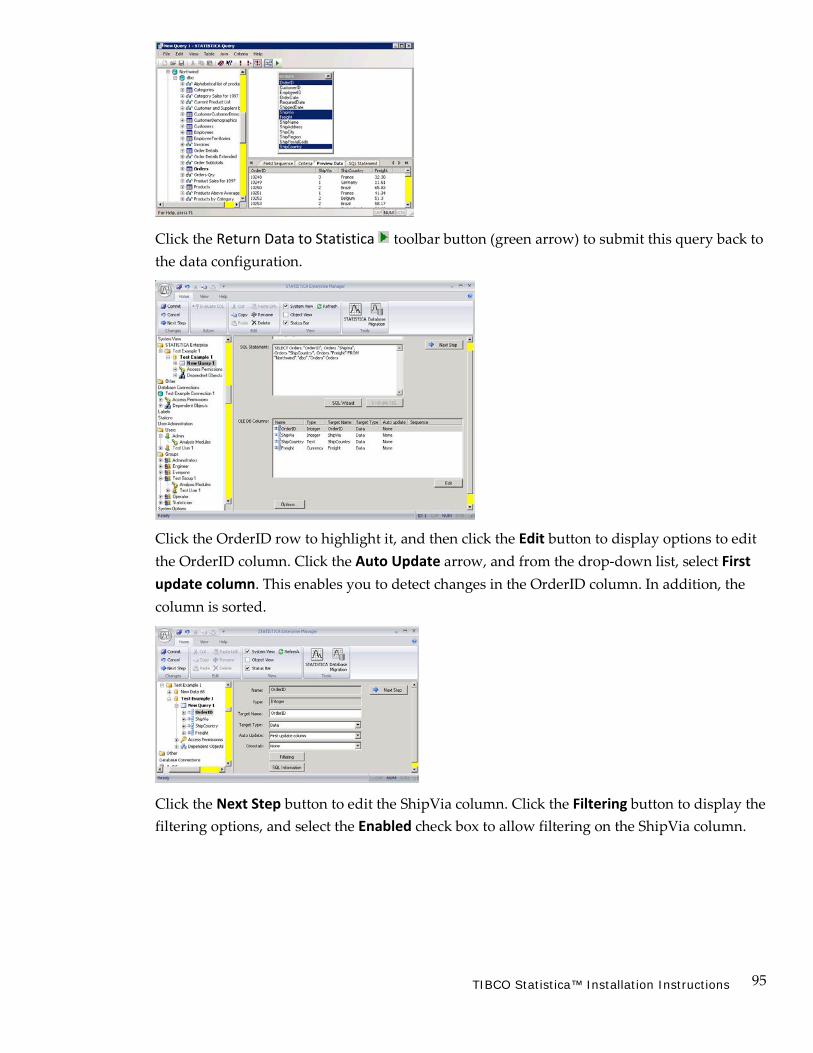
95 TIBCO Statistica™ Installation Instructions
Click the Return Data to Statistica toolbar button (green arrow) to submit this query back to the data configuration.
Click the OrderID row to highlight it, and then click the Edit button to display options to edit the OrderID column. Click the Auto Update arrow, and from the drop-down list, select First update column. This enables you to detect changes in the OrderID column. In addition, the column is sorted.
Click the Next Step button to edit the ShipVia column. Click the Filtering button to display the filtering options, and select the Enabled check box to allow filtering on the ShipVia column.
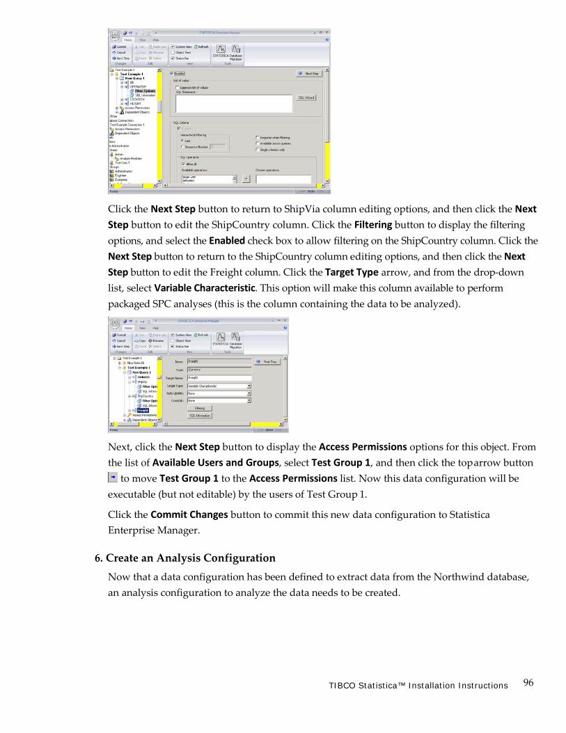
96 TIBCO Statistica™ Installation Instructions
Click the Next Step button to return to ShipVia column editing options, and then click the Next Step button to edit the ShipCountry column. Click the Filtering button to display the filtering options, and select the Enabled check box to allow filtering on the ShipCountry column. Click the Next Step button to return to the ShipCountry column editing options, and then click the Next Step button to edit the Freight column. Click the Target Type arrow, and from the drop-down list, select Variable Characteristic. This option will make this column available to perform packaged SPC analyses (this is the column containing the data to be analyzed).
Next, click the Next Step button to display the Access Permissions options for this object. From the list of Available Users and Groups, select Test Group 1, and then click the top arrow button
to move Test Group 1 to the Access Permissions list. Now this data configuration will be executable (but not editable) by the users of Test Group 1.
Click the Commit Changes button to commit this new data configuration to Statistica Enterprise Manager.
6. Create an Analysis Configuration Now that a data configuration has been defined to extract data from the Northwind database, an analysis configuration to analyze the data needs to be created.
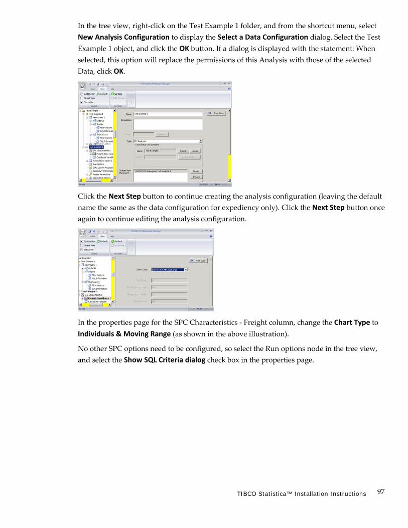
97 TIBCO Statistica™ Installation Instructions
In the tree view, right-click on the Test Example 1 folder, and from the shortcut menu, select New Analysis Configuration to display the Select a Data Configuration dialog. Select the Test Example 1 object, and click the OK button. If a dialog is displayed with the statement: When selected, this option will replace the permissions of this Analysis with those of the selected Data, click OK.
Click the Next Step button to continue creating the analysis configuration (leaving the default name the same as the data configuration for expediency only). Click the Next Step button once again to continue editing the analysis configuration.
In the properties page for the SPC Characteristics - Freight column, change the Chart Type to Individuals & Moving Range (as shown in the above illustration).
No other SPC options need to be configured, so select the Run options node in the tree view, and select the Show SQL Criteria dialog check box in the properties page.
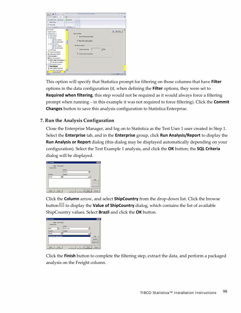
98 TIBCO Statistica™ Installation Instructions
This option will specify that Statistica prompt for filtering on those columns that have Filter options in the data configuration (if, when defining the Filter options, they were set to Required when filtering, this step would not be required as it would always force a filtering prompt when running – in this example it was not required to force filtering). Click the Commit Changes button to save this analysis configuration to Statistica Enterprise.
7. Run the Analysis Configuration Close the Enterprise Manager, and log on to Statistica as the Test User 1 user created in Step 1. Select the Enterprise tab, and in the Enterprise group, click Run Analysis/Report to display the Run Analysis or Report dialog (this dialog may be displayed automatically depending on your configuration). Select the Test Example 1 analysis, and click the OK button; the SQL Criteria dialog will be displayed.
Click the Column arrow, and select ShipCountry from the drop-down list. Click the browse button to display the Value of ShipCountry dialog, which contains the list of available ShipCountry values. Select Brazil and click the OK button.
Click the Finish button to complete the filtering step, extract the data, and perform a packaged analysis on the Freight column.

99 TIBCO Statistica™ Installation Instructions
Custom User Interfaces Note that this simple example illustrates how to enable and run an analysis configuration using the standard Statistica user interface and output components.
However, one of the major strengths of Statistica Enterprise is the ease of creating custom user interfaces (for example, for different categories of users depending on their roles in the organization, expertise, or data access privileges).
You can easily create a customized user interface at any degree of complexity, from highly simplified ones, for example, one that contains only three options:
to very elaborate user interfaces of virtually unlimited flexibility:

100 TIBCO Statistica™ Installation Instructions
Please refer to the Statistica Enterprise documentation (Electronic Manual) for more details and examples.
The Statistica Enterprise Server Option Statistica Enterprise Server provides all of the functionality described in this example and also enables offloading tasks to the server and remote access via a browser interface.
See Appendix A – Statistica Enterprise Server.
101 TIBCO Statistica™ Installation Instructions
Chapter Three: User Interface
102 TIBCO Statistica™ Installation Instructions
General Features Customized Operation
The Statistica system can be controlled in several ways. The following sections summarize the features of the main alternative user interfaces of Statistica:
1. Interactive interface
2. Statistica Visual Basic
3. Web browser-based interfaces
4. Microsoft Office Integration
However, note that:
• Many aspects of these user interfaces do not exclude each other; thus, depending on your specific applications and preferences, you can combine them;
• The customizable Quick Access Toolbar and classic menus can be used to integrate the alternative user interfaces and, for example, to provide quick access to macro (Visual Basic) programs or commonly used files; and
• Almost all features of these alternative user interfaces can be customized (leading to a different appearance and behavior of Statistica); it is generally recommended that you customize your system in order to take full advantage of Statistica’s potential to meet your preferences and optimal requirements of the tasks that you need to accomplish.
Alternative Access to the Same Facilities - Custom Styles of Work Even without any customization, the default settings of Statistica offer alternative user interface means and solutions to achieve the same results. This “alternative access” principle present in every aspect of its user interface enables Statistica to support different styles of work. For example, most of the commonly used tools can be accessed alternatively:
• From the ribbon bar or the classic menus • Via keyboard shortcuts • By using the clickable fields on the status bar • Via the custom Quick Access toolbar (user-defined toolbar with buttons and special
controls, which can include macros and commands) • From the shortcut menus associated with specific objects (cells, workbook icons, parts
of graphs), which are displayed by right-clicking on the item.
It is suggested that you explore the alternative user interface facilities of Statistica before becoming attached to one style or another.

103 TIBCO Statistica™ Installation Instructions
Multiple Analysis Support As mentioned before, you can have several instances of Statistica open at the same time. Each of them can run the same or different types of analyses (traditionally called modules), such as Basic Statistics, Multiple Regression, ANOVA, etc.
Moreover, in one Statistica instance, multiple analyses can be open simultaneously. They can be of the same or a different kind (for example, five Multiple Regressions and two ANOVAs), and each of them can be performed on the same or a different input data file (multiple input data files can be opened simultaneously).
Individual analyses – functional units of your work. In order to facilitate taking advantage of this multitasking functionality, your work with Statistica is organized into functional units called analyses that are represented with buttons on the analysis bar at the bottom of the application window (above the status bar, see the following illustration, where Descriptive Statistics, Cluster Analysis, and Canonical Analysis are running simultaneously). Consecutive buttons are added as you start new analyses. A variety of options are provided to control (and/or permanently configure) this aspect of Statistica.
By default, when you select specific output from a results dialog, the output (a spreadsheet or a graph) is displayed and the dialog is automatically minimized into its respective analysis button at the bottom of the screen. Click that button (or press CTRL+R) to display the dialog again and resume the analysis.
A selection of options pertaining to analysis management are available on the shortcut menu (accessed by right-clicking on an analysis button on the analysis bar) related to each respective analysis button (as shown above).

104 TIBCO Statistica™ Installation Instructions
A useful hint for those with large screens. If you have a large screen, you can turn off the default minimization of the analysis dialogs and take advantage of the fact that most of these dialogs are small and, thus, can remain on the workspace without interfering with the viewing of analysis results. You can adjust this option either for a particular analysis (clear the Auto Minimize command on the analysis button shortcut menu, shown in the previous image), or globally for the entire program [select Analyses/Graphs in the tree pane of the Options dialog (accessible by selecting the Tools tab and clicking Options), and clear the Auto minimize dialogs when displaying output check box].
When you run multiple analyses and the Statistica workspace becomes cluttered, you can hide all windows related to specific analyses (or close them altogether via the analysis button shortcut menu command Close All Analyses). You can also open new Statistica instances, which offers another simple way to organize and manage your work.
Interactive User Interface
Overview Main components of the interactive user interface of Statistica. Although the interactive user interface of Statistica is not the only one available, in most cases it is the easiest and most commonly used. Many components of this user interface can be seen in the Statistica application window.
First, similar to most software programs, tabs, menu bars and various toolbars are displayed at the top of the window. These are customizable and displayed in the most appropriate manner for your tasks.
At the bottom of the window, the analysis bar (containing minimized analysis/graph dialogs) and the status bar are displayed. Additionally, shortcut menus are available when you right- click in appropriate places.
Data files can be displayed in spreadsheets, workbooks, reports, or individual windows. Results spreadsheets or graphs can be displayed in workbooks, reports, or individual windows. Note that additional documents (such as Word or Bitmap images) can also be displayed in spreadsheets, workbooks, or reports. Finally, Statistica Visual Basic code is displayed in macro windows.
Normally you would not simultaneously see all of these facilities and tools at one time. You always have the ability to make the user interface of Statistica as simple or complex as your particular needs and comfort level demand.

105 TIBCO Statistica™ Installation Instructions
Modules. While Statistica offers a variety of statistical and graphical procedures, each procedure can be performed in the same instance of Statistica. This means that, for example, it is possible to calculate residual statistics using options in the Multiple Regression module, then immediately use that output in the Factor Analysis or another exploratory module without first starting another instance of Statistica.
The Flow of Interactive Analysis Startup Panel. When a statistical procedure is selected from the Statistics, Data Mining, or Graphs tabs, its respective Startup Panel is displayed (as shown below; Basic Statistics was selected from the Statistics tab - Base group to display the Basic Statistics and Tables Startup Panel).
Each Startup Panel contains a list of the types of analyses available in that particular module. Clicking anywhere outside the panel automatically minimizes it as a button on the analysis bar. If your system includes a high-resolution screen, you can change this default and keep the consecutive dialogs (in each analysis sequence) displayed on the workspace.
Analysis specification and output selection (results) dialogs. When the desired analysis is selected in the Startup Panel, the analysis specification dialog is displayed, in which you select the variables to be analyzed and other options and features of the task to be performed. Often, these dialogs contain several tabs that group the options, analyses, and/or results in logical categories to make it easier to locate specific features.

106 TIBCO Statistica™ Installation Instructions
In some simple analyses (such as Descriptive Statistics, shown in the illustration above), the analysis specification dialog also serves as an output selection dialog where you can specify the type and format of the output (for example, specific spreadsheets or graphs). Most analyses, however, have a separate analysis specification dialog and results dialog.
Spreadsheet facilities for scenario (what-if) analyses and customized appearance. Statistica provides you with the capability to append supplementary information about variable measurement types and case states to your spreadsheets.
This metadata can be used to create a more comprehensive description of your data set, facilitate what-if types of exploratory analyses, and customize the appearance of cases in graphs.
Case states and brushing. You can assign case states to cases in order to customize the appearance of points in graphical displays, thus making it very easy to identify influential and interesting points.
A wide selection of symbols and colors is available to customize the appearance of selected points. Not only can case states be assigned in the spreadsheet before a graph is created, they can also be assigned interactively in the graph via the Brushing facilities (accessible by clicking the Brushing button in the Customize Graph group on the Edit tab when a graph is displayed).
The case states assigned in the graph propagate back to the spreadsheet. The ability to assign case states in either the spreadsheet or graph further facilitates the exploratory visual analysis of data.
Measurement types and automatic variable pre-screening. The modeling or measurement type of a variable can be explicitly defined in order to indicate what analyses and graphs are appropriate for such a variable. These measurement types will map directly to subsequent analyses and graphs, identifying appropriate variables in each case (for example, variables of type categorical will be present within the list of categorical predictors available in a Factorial ANOVA).

107 TIBCO Statistica™ Installation Instructions
In all variable selection dialogs (such as the one shown above), the Show appropriate variables only option is provided, which enables you to pre-screen or filter variables according to their Measurement Type (specified in the Variable specification dialog, accessible by double- clicking on a variable header in a spreadsheet); if that type is Auto, then the Automatic variable pre-screening and classification options (located in the Analysis/Graph options pane of the Options dialog, accessible by selecting the Tools tab and clicking Options) determine how Statistica will automatically determine the Measurement Type.
Auto filtering (cloaking variables and cases). Filtering (accessible by selecting the Data tab and clicking Auto Filter in the Transformations group) is a quick and easy way to display a specific portion of the data in your spreadsheet without sorting the data or creating a subset. When a variable is filtered, only the values that meet the specified criteria are displayed in the spreadsheet. Cases that do not meet the criteria are hidden from sight but not removed from the spreadsheet (for example, in the spreadsheet shown below, only the cases for GENDER = MALE are displayed).
Although hidden, they are still available for statistical and graphical analyses.
Output. As described in more detail in Chapter 4 – Five Channels for Output From Analyses and as illustrated in Example 1: Correlations (page 11) and Example 2: ANOVA (page 27), the consecutive output spreadsheets and graphs are displayed in workbooks by default. These workbooks can be saved and later reopened, making it easy to return to specific results as needed.
Additionally, you can send all output to an analysis report (see page 120), which produces an easily organized (via the report tree), formatted, and printed report of a specific analysis. You can also choose to send all results, regardless of what analysis it comes from, to a single report. Lastly, the output can be directed to separate windows.
To specify output options for a single analysis or session, click the button in the analysis or graph specification dialog and select Output to display the Analysis/Graph Output Manager dialog.
To access global output options, select the Tools tab. Click Options to display the Options dialog, and select Output Manager. Or, select the Home tab and click Options in the Tools group. For more information, see the Electronic Manual.
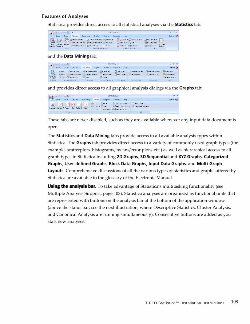
108 TIBCO Statistica™ Installation Instructions
Features of Analyses Statistica provides direct access to all statistical analyses via the Statistics tab:
and the Data Mining tab:
and provides direct access to all graphical analysis dialogs via the Graphs tab:
These tabs are never disabled, such as they are available whenever any input data document is open.
The Statistics and Data Mining tabs provide access to all available analysis types within Statistica. The Graphs tab provides direct access to a variety of commonly used graph types (for example, scatterplots, histograms, means/error plots, etc.) as well as hierarchical access to all graph types in Statistica including 2D Graphs, 3D Sequential and XYZ Graphs, Categorized Graphs, User-defined Graphs, Block Data Graphs, Input Data Graphs, and Multi-Graph Layouts. Comprehensive discussions of all the various types of statistics and graphs offered by Statistica are available in the glossary of the Electronic Manual
Using the analysis bar. To take advantage of Statistica’s multitasking functionality (see Multiple Analysis Support, page 103), Statistica analyses are organized as functional units that are represented with buttons on the analysis bar at the bottom of the application window (above the status bar, see the next illustration, where Descriptive Statistics, Cluster Analysis, and Canonical Analysis are running simultaneously). Consecutive buttons are added as you start new analyses.

109 TIBCO Statistica™ Installation Instructions
Minimizing dialogs (and a hint for users with large screens). Depending on your preferences, you can choose to minimize all analysis dialogs when you select another window in Statistica or another application. By default the Auto Minimize command is selected; however, when your screen is large enough to accommodate several windows, it is recommended that you clear this command.
This keeps the analysis dialogs on screen while the respective output created from these dialogs is produced, thus enabling you to use the dialogs as “toolbars” from which output can be selected. See page 104 for information on how to adjust this command.
Continuing analyses/graphs. It is easy to continue an analysis or graph (such as to change the focus to the current dialog for a particular analysis). Select the Tools tab, click Analysis Bar, and select Resume from the drop-down menu; or press CTRL+R; or click the analysis/graph button on the analysis bar. When multiple analyses are running, you can also select the specific analysis from the Select Analysis/Graph submenu (as shown in the next illustration).

110 TIBCO Statistica™ Installation Instructions
Hiding windows. To further facilitate the organization of windows from various analyses, you can hide all windows associated with a particular analysis when that analysis is deselected: select the Tools tab, click Analysis Bar, and from the Options submenu, select Hide on Deselect. By default, this command is not selected. Note that this command only applies when the results are sent to individual windows; see the discussion of the Output Manager for more details on managing output from analyses. In addition, there is a command on the Home tab in the Windows group to close all document windows: click Close All (or press CTRL+L on your keyboard), and a command on the Tools tab to close all analyses: click Analysis Bar and select Close All Analyses from the drop-down menu.
Bringing windows to the top. On the Tools tab click Analysis Bar, and from the Options submenu select Bring to Top on Select to activate (bring to the top of Statistica) all windows associated with a particular analysis when that analysis is selected, replacing whatever dialogs were on top.
This command also facilitates the organization of individual windows from various analyses. By default, this command is selected. Note that this command only applies when the results are sent to individual windows; see the discussion of the Output Manager for more details on managing output from analyses.
Hiding the summary box. By default, a summary box is located at the top of certain results dialogs (such as Multiple Regression Results) and contains basic summary information about the analysis. You can hide an individual summary box by clicking the button in the lower- right corner of the summary box. You can also suppress the display of all summary boxes globally by selecting the Tools tab, clicking Analysis Bar, and selecting Hide Summary Box from the Options submenu.
Document Types Statistica uses seven principal document types:
• Workbooks • Spreadsheets (multimedia tables) • Reports • Graphs • Macros (Statistica Visual Basic programs) Statistica Project Files • Data Miner Recipes Project Files (see page 51)
Using these seven document types, you can manage data of various types, perform data entry and analyses, generate graphs of the highest quality, develop custom applications of any degree of complexity, and create custom-formatted reports.
You can quickly access the most recently used documents. Click the Statistica Start menu (in the lower-left corner of the screen) and select Documents.
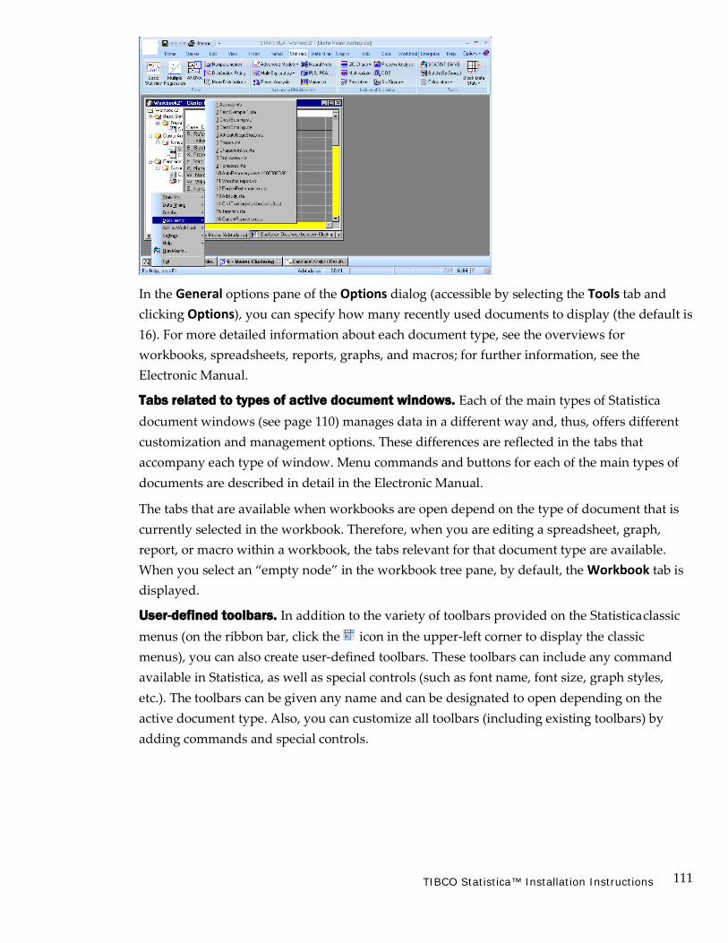
111 TIBCO Statistica™ Installation Instructions
In the General options pane of the Options dialog (accessible by selecting the Tools tab and clicking Options), you can specify how many recently used documents to display (the default is 16). For more detailed information about each document type, see the overviews for workbooks, spreadsheets, reports, graphs, and macros; for further information, see the Electronic Manual.
Tabs related to types of active document windows. Each of the main types of Statistica document windows (see page 110) manages data in a different way and, thus, offers different customization and management options. These differences are reflected in the tabs that accompany each type of window. Menu commands and buttons for each of the main types of documents are described in detail in the Electronic Manual.
The tabs that are available when workbooks are open depend on the type of document that is currently selected in the workbook. Therefore, when you are editing a spreadsheet, graph, report, or macro within a workbook, the tabs relevant for that document type are available. When you select an “empty node” in the workbook tree pane, by default, the Workbook tab is displayed.
User-defined toolbars. In addition to the variety of toolbars provided on the Statistica classic menus (on the ribbon bar, click the icon in the upper-left corner to display the classic menus), you can also create user-defined toolbars. These toolbars can include any command available in Statistica, as well as special controls (such as font name, font size, graph styles, etc.). The toolbars can be given any name and can be designated to open depending on the active document type. Also, you can customize all toolbars (including existing toolbars) by adding commands and special controls.

112 TIBCO Statistica™ Installation Instructions
To create a toolbar (or edit an existing one) use the options on the Toolbars tab of the Customize dialog, accessible by selecting Customize from the Tools menu. Customizing a toolbar is as easy as dragging commands from the dialog to the toolbar, as shown in the illustration below.
Shapes and locations of toolbars can be easily adjusted (for example, all toolbars can be docked or free floating). All of these options make it possible for you to create unique toolbars that provide you with a very specialized user interface. The Electronic Manual includes simple-to- follow, step-by-step instructions on how to make customizations. Specifically, see Create a New Toolbar in the Electronic Manual for more details.
The Quick Access toolbar located at the top of the ribbon bar can be customized as well; see Customize Quick Access Toolbar in the Electronic Manual.
User-defined menus. Customizing the classic menus is equally easy and can be performed using the Menu tab of the Customize dialog (see the Electronic Manual for details).
Statistica Visual Basic and Controlling Statistica from Other Applications
The industry standard Statistica Visual Basic language (integrated into Statistica) provides an alternative user interface to the entire functionality of Statistica, and it offers incomparably more than just a supplementary application programming language that can be used to write custom extensions.
Statistica Visual Basic takes full advantage of the object model architecture of Statistica and can be used to access programmatically every aspect and virtually every detail of the functionality of Statistica.
113 TIBCO Statistica™ Installation Instructions
Even the most complex analyses and graphs can be recorded into Visual Basic macros and later be run repeatedly or edited and used as building blocks of other applications. Statistica Visual Basic adds an arsenal of more than 14,000 new functions to the standard comprehensive syntax of Visual Basic, thus comprising one of the largest and richest development environments available. For more information on Statistica Visual Basic, see Chapter 8
Controlling Statistica from other applications. One of the features that makes the Statistica Visual Basic environment so powerful is the ability to integrate and manipulate various applications and their environments within a single macro. For example, you can record or write a Statistica Visual Basic program that computes predictions via the Statistica Time Series module and execute that program from within an Excel spreadsheet or a Word document. The exchange of information between different applications is accomplished by exposing those applications to the Visual Basic programs as Objects. So, for example, you can run statistical analyses in the Statistica Basic Statistics module from a Visual Basic program in Excel by declaring inside the program an object of type Statistica.Application.
Once an object has been created, the Visual Basic program then has access to the properties and methods contained in that object. Properties can be mostly thought of as functions, methods can be mostly thought of as subroutines that perform certain operations or computations inside the respective application object. You can call Statistica procedures directly from many other applications and programming languages (for example, C++, Java, and others).
Web Browser-Based User Interface: Statistica Enterprise Server
In addition to the two basic types of user interfaces described in the previous sections, the entire Statistica family of products also optionally offers a browser-based user interface, where all interactions with the application involving querying databases, data management operations, data analysis, or data mining, as well as generating reports and collaborative work, can be performed without having any Statistica application installed on the local computer, using only a browser. This alternative user interface requires that a Client-Server version of the respective Statistica application be installed.

114 TIBCO Statistica™ Installation Instructions
Statistica Enterprise Server is a highly scalable, enterprise-level, fully Web-enabled data analysis and database gateway application system that is built on distributed processing technology and fully supports multi-tier Client-Server architecture configurations. Statistica Enterprise Server exposes the analytic, query, reporting, and graphics functionality of Statistica through easy-to-use, interactive, standard Web interfaces. Alternatively, it enables users of the desktop version (“thick client”) to offload computationally intensive analytics and database operations to the Server. It is offered as a complete, ready-to-install application with an interactive, Internet browser-based (“point-and-click”) user interface (“thin client”) that makes it possible for users to interactively create data sets, run analyses, and review output. However, Statistica Enterprise Server is built using open architecture and includes .NET-compatible development kit tools (based entirely on industry standard syntax conventions such as VB Script, C++/C#, HTML, Java, and XML) that enables IT department personnel to customize all main components of the system or expand it by building on its foundations, for example, by adding new components and/or company-specific analytic or database facilities.
As mentioned, Statistica Server is provided with an Internet browser-based user interface (in the form of simple-to-navigate and easy-to-use dialogs) enabling you to specify analyses and review results.
However, tools are provided to customize these dialogs and easily set up new user interfaces or to add new functions. For example, a simple dialog with only three buttons can be created in the browser, and clicking each button will run a series of analyses and generate a detailed report. Statistica Enterprise Server applications add a new dimension and an endless array of possibilities to the entire line of Statistica Data Analysis, Data Mining, and Quality Control/Six Sigma software.
The system is compatible with all major Web server software platforms (for example, UNIX Apache, and Microsoft IIS), works in both Microsoft .NET and Sun/Java environments, and does not require any changes to the existing firewall and Internet/Intranet security systems
For more information, please refer to Appendix A – Statistica Enterprise Server.
Microsoft Office integration If Microsoft Office is installed on the same machine as Statistica, Excel spreadsheets can be opened directly within Statistica and used as a data source for analyses, and Word documents can be used as a destination for reports (see page115; see also page 123).
Excel as a data source. Statistica can open Excel documents in the Statistica workspace through the standard Open dialog. When an Excel workbook is selected, a dialog will be displayed that enables you to import the file into a standard Statistica Spreadsheet or to keep the document in Excel form, such as as an Excel window within Statistica.

115 TIBCO Statistica™ Installation Instructions
Once the Excel document is opened, you have access to all the menus and toolbars that Excel supports. Thus, you can edit and update formulas, change the formatting, copy/paste, drag/drop – everything that you would normally do if you were within the Excel application.
The main strength in Excel integration is that the Excel documents can be used as a data source for analyses. Simply have the Excel document window selected when starting an analysis, and the analysis will source from the Excel document.
When initially running the analysis, Statistica will display a dialog in which you can specify what range of the Excel document should be used as the data source and if a particular row or column is to be used as variable names or case names. These settings are assigned to the Excel document so you will only need to specify them once.
Not only can Statistica use the Excel file as a data source, but auto updating can be specified as well. If you create an auto-updating graph and then change the Excel file by entering new data or re-evaluating formulas, the graph will also be updated.
Word as a report destination. You can also open and edit Word documents within the Statistica workspace. Word documents can be opened using the standard Open dialog, and when performing statistical analyses or creating graphs, output can being directed to a Word document. Any output that can be directed to a Statistica Report is capable of being directed to a Word document.
As with Excel, when the Word document is open, you have access to all the toolbars and menus that are supported within the Word application. You can perform any formatting and editing that Word supports within its application.
When sending spreadsheet analytical results to Word, Statistica will take advantage of Word’s table editing facility and convert the spreadsheet into a table. For multi-page spreadsheets, you can control where to break the rows and columns.
These spreadsheets will be broken by columns such as will be allowed without exceeding the page width. All rows for a given set of columns will be rendered before the next set of spreadsheet columns is rendered in the Word document. This solution enables the presentation of spreadsheets in Word that are natively editable in Word, display the entire contents of the spreadsheet, and print and paginate correctly.

116 TIBCO Statistica™ Installation Instructions
Chapter Four Six Channels for Output from Analyses

117 TIBCO Statistica™ Installation Instructions
Overview
When you perform an analysis, Statistica generates output in the form of multimedia tables (spreadsheets) and graphs. There are six basic channels to which you can direct all output:
1. Statistica Workbooks (page 118)
2. Stand-alone Windows (page 119)
3. Reports (page 120)
4. Microsoft Word (page 123)
5. The Web (page 124)
6. SharePoint or Statistica Document Management System (SDMS) (page 129)
The first four output channels listed above are controlled by the options in the Output Manager (accessible by selecting Output Manager from the Start button drop-down menu located in the upper-left corner of the ribbon bar, see page 20 for further details on both the global Output Manager in the Options dialog and the Analysis/Graph Output Manager dialog). There are a number of ways to output to the Web, depending on the version of Statistica you have. SharePoint is accessible from within Statistica, and SDMS is an additional product available from Statistica.
These means for output can be used in many combinations (for example, a workbook and report simultaneously) and can be customized in a variety of ways. Also, all output objects (spreadsheets and graphs) placed in each of the output channels can contain other embedded and linked objects and documents, so Statistica output can be hierarchically organized in a variety of ways. Each of the Statistica output channels has its unique advantages, as described in the following sections. More comprehensive overviews of each of the document types associated with the respective channels of output are included in Chapter 5 - Statistica Documents.
The auto save and recovery features. All Statistica documents (such as input spreadsheets, workbooks, reports, and macros) that accumulate the results of your work (for example, data entry, editing, or output collection) over an extended period of time support the Auto Save feature, which is configurable in the General options pane of the Options dialog (accessible by selecting the Tools tab and clicking Options).
This facility will automatically save the contents of your work periodically (for example, every 10 minutes) and, thus, give you the option to retrieve data that otherwise could be lost in case of a power outage or a system failure.

118 TIBCO Statistica™ Installation Instructions
1. Statistica Workbooks Workbooks are the default way of managing output (for more information). Each output document (for example, a Statistica Spreadsheet or Graph, as well as a Word or Excel document) is stored as a tab in the workbook.
Documents can be organized into hierarchies of folders or document nodes (by default, one is created for each new analysis) using a tree view, in which individual documents, folders, or entire branches of the tree can be flexibly managed.
For example, selections of documents can be extracted (for example, drag-copied or drag- moved) to a report window or to the application workspace (such as the Statistica application background where they will be displayed in stand-alone windows). Entire branches can be placed into other workbooks in a variety of ways in order to build specific folder organization, etc.
Technically speaking, workbooks are ActiveX document containers (see page 184 for information on ActiveX technology, see also the Electronic Manual). Workbooks are compatible with a variety of foreign file formats (for example, Office documents) that can be easily inserted into workbooks and in-place edited.
User notes and comments in workbooks. Workbooks offer powerful options to efficiently manage even extremely large amounts of output, and they may be the best output handling solution for both novices and advanced users. It might appear that one possible drawback is that user comments (for example, notes) and supplementary information cannot be as transparently inserted into the “stream” of the workbook output as they can in traditional, word processor style reports, such as Statistica Reports (see the next section). However, note that:
• All Statistica documents can easily be annotated, both a) directly, by typing text into graphs, tables, and reports, and b) indirectly, by entering notes into the Comments box of the Document Properties dialog (accessed by selecting Properties from the Start
button drop-down menu located in the upper-left corner of the ribbon bar), and

119 TIBCO Statistica™ Installation Instructions
• Formatted documents with notes and comments (in the form of text files, Statistica Report documents, WordPad or word processor documents, etc.) can easily be inserted anywhere in the hierarchical organization of output in workbooks. Moreover, such summary notes or comment documents can be made nodes for groups of subordinate objects to which the note is related to further enhance their organization.
Saving workbooks as Web pages. Workbooks can be saved as *.html (Web) files by selecting Save As on the Home tab in the File group from the Save menu, and in the Save As dialog, choosing Web Page (*.htm; *.html) from the Save as type drop-down list. Saving as a Web page will create an *.html file in the specified directory that can be opened with standard internet browsers such as Microsoft Internet Explorer. When saving the workbook as a Web page, Statistica also creates a subdirectory that contains all the images referenced by the Web page.
The Web page output contains an .html-based tree control that enables you to navigate and display the various workbook images, similar to the actual workbook.
2. Stand-Alone Windows Statistica output documents can also be directed to a queue of stand-alone windows; the Queue Length can be controlled in the Output Manager options pane of the Options dialog (accessible by selecting the Tools tab and clicking Options).
standalone2.bmp

120 TIBCO Statistica™ Installation Instructions
The clear disadvantage of this output mode is its total lack of organization and its natural tendency to clutter the application workspace (some procedures can generate hundreds of tables or graphs with a click of the button).
One of the advantages of this way of handling output is that you can easily custom arrange these objects within the Statistica application workspace (for example, to create multiple, easy to identify “reference documents” to be compared to the new output). However, note that in order to achieve that effect, you do not need to configure the output ahead of time and generate a large number of (mostly unwanted) separate windows that can clutter the workspace. Instead, individual, specific output objects directed to and stored in the other two channels (workbooks and reports) can easily be dragged out from their respective tree views onto the application workspace as needed.
3. Reports When performing an analysis, the ultimate goal is to create meaningful output in order to gain an understanding of the data. The manner in which the output is produced is important as well. Statistica offers a variety of methods to produce reports that accommodate the diverse needs of users.
Statistica Reports Statistica Reports (for more information, see page 143) offer a more traditional way of handling output where each object (for example, a Statistica Spreadsheet or Graph, or an Excel spreadsheet) is displayed sequentially in a word processor style document.
However, the technology behind this simple editor offers you very rich functionality. For example, like the workbook (see Statistica Workbooks, page 118), the Statistica Report is also an ActiveX container (for information on ActiveX technology, see page 184 or the Electronic Manual) where each of its objects (not only Statistica Spreadsheets and Graphs, but also any other ActiveX-compatible documents, for example, Excel spreadsheets) remains active, customizable, and in-place editable.
121 TIBCO Statistica™ Installation Instructions
The obvious advantages of this way of handling output (more traditional than the workbook) are the ability to insert notes and comments in between the objects as well as its support for the more traditional way of quick scrolling through and reviewing the output to which some users may be accustomed (for example, the editor supports variable speed scrolling).
Also, only the report output includes and preserves the record of the supplementary information, which contains a detailed log of the options specified for the analyses (for example, selected variables and their labels, long names, etc., depending on the level of supplementary information specified in the Output Manager, see page 21).
The obvious drawback, however, of these traditional reports is the inherent flat structure imposed by their word processor style format, although that is what some users or certain applications may favor.
Reports from Workbooks When you have a Statistica Workbook containing analyses output, you may decide you want to transfer it to a report.
Open a Statistica Workbook and select all of the files, such as select the first file, press the SHIFT
key on your keyboard, and select the last file. Then, click Add to Report on the Home tab in the Output group. All the files in the workbook will be duplicated in a Statistica Report.
RTF (Rich Text Format) Reports RTF (Rich Text Format) is a Microsoft standard method of encoding formatted text and graphics for easy transfer between applications. When reports are saved in Rich Text Format (*.rtf), all file formatting is preserved so that it can be read and interpreted by other RTF- compatible applications (for example, Word).
The Statistica Report format (.str) adheres to RTF conventions; however, saving reports in the default Statistica Report format ensures that the reports will be opened in Statistica, giving you complete access to the report tree.
In order to open a Statistica report in an RTF-compatible application, open the report, select the Home tab, click the Save arrow, and select Save As from the drop-down menu to display the Save As dialog. From the Save as type drop-down list, select Rich Text Files (*.rtf), enter a name in the File name field, and click the Save button. You can then open the file in any RTF- compatible application.

122 TIBCO Statistica™ Installation Instructions
Acrobat (PDF) Reports PDF is the acronym for Portable Document Format; it is the industry-standard format for storing textual and graphical data. PDF offers a graphically rich appearance and structure that makes it ideal for presentation purposes. Additionally, PDF documents can be viewed in both image and textual mode, such as you can either select data as a formatted image or as regular text.
PDF is platform independent, and most operating systems offer free PDF viewing applications (for example, Adobe Acrobat on Windows and Ghostscript on Linux).
PDF has been approved as an acceptable document storage format for regulated environments according to the FDA’s 21 CFR Part 11.
To save a Statistica Report as a PDF file, open the report, select the Home tab, and then select Save As PDF from the Save menu. The Output Options dialog will be displayed, where you can choose whether to output spreadsheets as Objects (as they are sized in the report window) or Full-sized Spreadsheets (on separate pages).
If you always want to output spreadsheets in the same manner, select the Use the current setting and do not display this dialog again check box. Click the OK button to close the Output Options dialog and display the Save report as PDF dialog. Use the Save in field to select the appropriate location in which to save the document, enter a name in the File name field, and click the Save button. Statistica Reports, Spreadsheets, and Graphs can all be saved in PDF format.
Note that these are not simplified PDF files (representing compressed bitmaps of the respective document page images) but full-featured PDF files that support such operations as selective copying of text information.
HTML Reports
You may want to post a Statistica Report or Workbook on the Internet for others to review. With Statistica, you can save reports and workbooks in HTML (an acronym for HyperText Markup Language) format. HTML uses tags to identify elements of the document, such as text or graphics.
Open a Statistica Report or Workbook, and select Save As from the Save menu (located on the Home tab in the File group) to display the Save As dialog. From the Save as type drop-down list, select Web Page (*.html; *.htm) to save the file with an *.htm extension.
Note that graphs in the report or workbook are saved as *.png files in the same folder as the HTM file. You can save graphs as JPG files, instead. To do this, click Options (on the Home tab in the Tools group) to display the Options dialog. Select either Reports or Workbooks in the tree view, according to which document you intend to send to an .htm document, select the JPEG format option button in the Export HTML images as group box, and click OK.
123 TIBCO Statistica™ Installation Instructions
4. Microsoft Word With Statistica, you can also route output directly to Word via the Office Integration features. When Word is open within Statistica, Word toolbars and menus are also available through standard Active X Document interfaces technology. In Statistica, you can perform any formatting and editing that Word supports in its application.
When sending spreadsheet analytical results to Word, Statistica will take advantage of Word’s table editing facility, and convert the spreadsheet to a table. For multi-page spreadsheets, you can control where to break the rows and columns. These spreadsheets will be broken by columns such as will be allowed without exceeding the page width. All rows for a given set of columns will be rendered before the next set of spreadsheet columns is rendered in the Word document. This solution enables the presentation of spreadsheets in Word that are natively editable in Word, displays the entire contents of the spreadsheet, and prints and paginates correctly.
As with standard Statistica Reports (see page 120), Word documents can store and preserve the record of supplementary information (for example, selected variables, long names, etc.).
To send output to a Word document, use the options in the Output Manager (accessible by
selecting Output Manager from the Start button drop-down menu located in the upper-left corner of the ribbon bar; or by selecting the Home tab, clicking Options in the Tools group, and selecting Output Manager in the Options dialog tree view). In the Microsoft Word Output drop-down list, select either Multiple Word documents (one for each analysis/graph), Common Word document (one shared for all analyses/graphs), or [Select File] to browse to a preexisting Word document.
Although Word documents do not provide the navigational tree of a Statistica Workbook or Report, the advantages in sending output to Word documents are many. By sending results to a Word document, you have all the word processing features of Word available. For example, you can attach templates to create customized documents, add tables of content and indices, track changes, etc.
When inserting a large spreadsheet into a Word document, Statistica automatically detects how many variables can fit on each page and partitions the spreadsheet into several Word tables. If the spreadsheet uses case names, those names will be the first column in each table.
Additional benefits of sending results to a Word document include increased printing functionality (for example, printing to files, manual duplex) and the ability to save results as Web pages.

124 TIBCO Statistica™ Installation Instructions
5. Output to the Web
Knowledge Portal
Statistica Enterprise Server Reports, or any Statistica Reports (see HTML Reports, page 122), can be distributed through the Knowledge Portal. The Knowledge Portal enables you to publish Statistica documents (spreadsheets, graphs, reports, or workbooks) to the Internet. Users with limited Knowledge Portal permissions can then view those documents. You can control who can access these documents by setting permissions on the documents and directories using standard Statistica Enterprise Server repository tools.
To publish content in the Knowledge Portal, first create a directory in the Statistica Enterprise Server repository in the Portal folder: log on to the Statistica Enterprise Server as a user with Administrator rights, and from the File menu, select My Directory Operations to display the My Directory dialog; the content will look similar to the following illustration.
To create a folder in the Portal directory to contain your reports, select the Portal folder, and then click the Create button to display the Explorer User Prompt dialog. In the edit field, enter the new directory name of Sample Portal Folder, and click OK. A dialog will be displayed confirming that the directory /Portal/Sample Portal Folder was created. Click the Show My Directory button, and you will be returned to the My Directory dialog. Select the Show Empty Directories check box, and then click the Refresh button. Expand the Portal directory by clicking the + next to that folder, and the new Sample Portal Folder will be displayed.
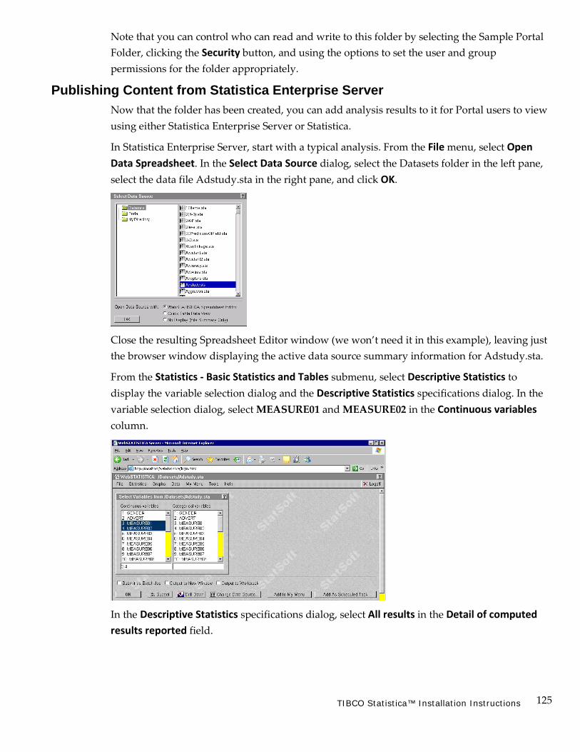
125 TIBCO Statistica™ Installation Instructions
Note that you can control who can read and write to this folder by selecting the Sample Portal Folder, clicking the Security button, and using the options to set the user and group permissions for the folder appropriately.
Publishing Content from Statistica Enterprise Server Now that the folder has been created, you can add analysis results to it for Portal users to view using either Statistica Enterprise Server or Statistica.
In Statistica Enterprise Server, start with a typical analysis. From the File menu, select Open Data Spreadsheet. In the Select Data Source dialog, select the Datasets folder in the left pane, select the data file Adstudy.sta in the right pane, and click OK.
Close the resulting Spreadsheet Editor window (we won’t need it in this example), leaving just the browser window displaying the active data source summary information for Adstudy.sta.
From the Statistics - Basic Statistics and Tables submenu, select Descriptive Statistics to display the variable selection dialog and the Descriptive Statistics specifications dialog. In the variable selection dialog, select MEASURE01 and MEASURE02 in the Continuous variables column.
In the Descriptive Statistics specifications dialog, select All results in the Detail of computed results reported field.

126 TIBCO Statistica™ Installation Instructions
Click OK to display the results for this analysis, consisting of several spreadsheets and graphs.
WebStat2
Now, to publish this page so that other users can see it from the Knowledge Portal, click the Publish button in the upper-right portion of the window. The Publish Destination dialog will be displayed. Here you can select the Sample Portal Folder that you created. You also can control who can have access to this particular page by selecting the I want to define who can access this output page check box.

127 TIBCO Statistica™ Installation Instructions
Click the Next button, and the page will be saved to the selected destination.
Now, when a Knowledge Portal user logs on, they will see the new Sample Portal Folder in their output browser, from which they can select the newly added Descriptive Statistics page.
Publishing Content from Statistica Desktop Applications With the Statistica Enterprise Server integration feature of desktop Statistica, you can also publish Statistica documents (spreadsheets, graphs, reports, and workbooks) to the Knowledge Portal directly from within the Statistica application.
The first step is to enable Statistica Enterprise Server integration. Select the Home tab, and in the Tools group click Options to display the Options dialog. Select Server/Web in the tree view, and in the options pane, select the Enable Statistica Enterprise Server Integration check box.
Then, specify the URL of the Statistica Enterprise Server and any optional custom configuration settings that may have been defined by your system administrator when installing Statistica Enterprise Server. In the following illustration, Statistica Enterprise Server has been installed on serverx23; the information in your dialog will be different depending on where Statistica Enterprise Server is installed on your network.
After you click the OK button in the Options dialog, note that there is a now a Server tab displayed in Statistica next to the Home tab. The only command on the Server tab that is available initially is Log In; select that command. If you have enabled integrated log in (and your Windows account is enabled on the Statistica Enterprise Server), you will be logged in automatically. Otherwise, you will be prompted for a Statistica Enterprise Server user name and password. Once you have logged in, the other commands are available on the Server tab.
Now, we will create an analysis and upload the results to the Knowledge Portal. Open the Adstudy.sta data file: select the Home tab, click the Open arrow, and select Open Examples from the drop-down menu; in the Open a Statistica Data File dialog, double-click on the Datasets folder, and then double-click on the Adstudy.sta file to open that spreadsheet for use in Statistica.

128 TIBCO Statistica™ Installation Instructions
Next, select the Statistics tab, and in the Base group, click Basic Statistics to display the Basic Statistics and Tables Startup Panel. Select Descriptive statistics.
Click OK to display the Descriptive Statistics dialog.
To ensure that all the output from this analysis will be sent to a workbook, click the Options button on the right side of the dialog, and from the drop-down list, select Output. In the Analysis/Graph Output Manager, verify that the Workbook option button is selected in the Place all results (Spreadsheets, Graphs) in group box. Then click OK to return to the Descriptive Statistics dialog.
Click the Variables button to display the variable selection dialog, select MEASURE01 and MEASURE02, and click OK to return to the Descriptive Statistics dialog. On the Quick tab, click the Summary: Statistics button to send those results to the workbook.
The Descriptive Statistics dialog will be minimized so you can see the results; restore it by clicking the Descriptive Statistics button on the Analysis Bar in the lower-left of the screen. Now click the Histograms button to generate histograms for each selected variable. The analysis dialog is minimized again, and the workbook should look as follows.
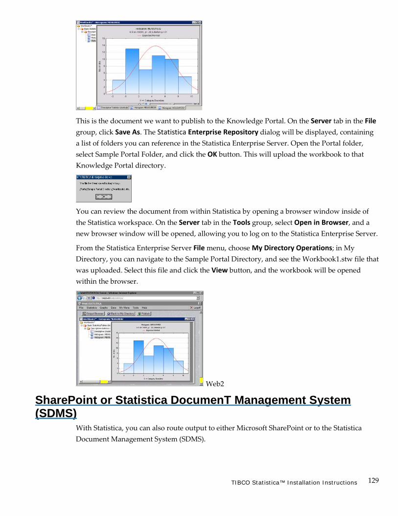
129 TIBCO Statistica™ Installation Instructions
This is the document we want to publish to the Knowledge Portal. On the Server tab in the File group, click Save As. The Statistica Enterprise Repository dialog will be displayed, containing a list of folders you can reference in the Statistica Enterprise Server. Open the Portal folder, select Sample Portal Folder, and click the OK button. This will upload the workbook to that Knowledge Portal directory.
You can review the document from within Statistica by opening a browser window inside of the Statistica workspace. On the Server tab in the Tools group, select Open in Browser, and a new browser window will be opened, allowing you to log on to the Statistica Enterprise Server.
From the Statistica Enterprise Server File menu, choose My Directory Operations; in My Directory, you can navigate to the Sample Portal Directory, and see the Workbook1.stw file that was uploaded. Select this file and click the View button, and the workbook will be opened within the browser.
Web2
SharePoint or Statistica DocumenT Management System (SDMS)
With Statistica, you can also route output to either Microsoft SharePoint or to the Statistica Document Management System (SDMS).
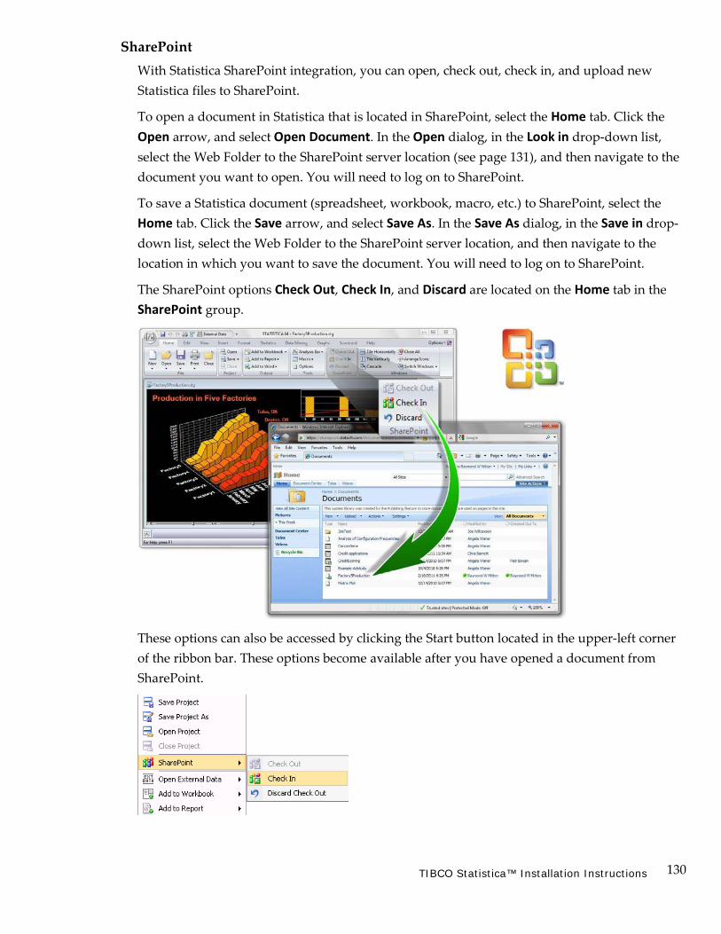
130 TIBCO Statistica™ Installation Instructions
SharePoint With Statistica SharePoint integration, you can open, check out, check in, and upload new Statistica files to SharePoint.
To open a document in Statistica that is located in SharePoint, select the Home tab. Click the Open arrow, and select Open Document. In the Open dialog, in the Look in drop-down list, select the Web Folder to the SharePoint server location (see page 131), and then navigate to the document you want to open. You will need to log on to SharePoint.
To save a Statistica document (spreadsheet, workbook, macro, etc.) to SharePoint, select the Home tab. Click the Save arrow, and select Save As. In the Save As dialog, in the Save in drop- down list, select the Web Folder to the SharePoint server location, and then navigate to the location in which you want to save the document. You will need to log on to SharePoint.
The SharePoint options Check Out, Check In, and Discard are located on the Home tab in the SharePoint group.
These options can also be accessed by clicking the Start button located in the upper-left corner of the ribbon bar. These options become available after you have opened a document from SharePoint.
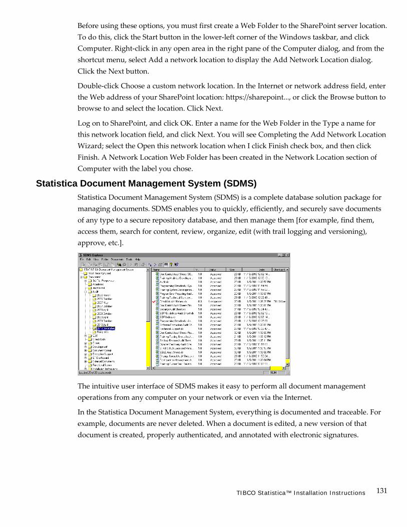
131 TIBCO Statistica™ Installation Instructions
Before using these options, you must first create a Web Folder to the SharePoint server location. To do this, click the Start button in the lower-left corner of the Windows taskbar, and click Computer. Right-click in any open area in the right pane of the Computer dialog, and from the shortcut menu, select Add a network location to display the Add Network Location dialog. Click the Next button.
Double-click Choose a custom network location. In the Internet or network address field, enter the Web address of your SharePoint location: https://sharepoint..., or click the Browse button to browse to and select the location. Click Next.
Log on to SharePoint, and click OK. Enter a name for the Web Folder in the Type a name for this network location field, and click Next. You will see Completing the Add Network Location Wizard; select the Open this network location when I click Finish check box, and then click Finish. A Network Location Web Folder has been created in the Network Location section of Computer with the label you chose.
Statistica Document Management System (SDMS) Statistica Document Management System (SDMS) is a complete database solution package for managing documents. SDMS enables you to quickly, efficiently, and securely save documents of any type to a secure repository database, and then manage them [for example, find them, access them, search for content, review, organize, edit (with trail logging and versioning), approve, etc.].
The intuitive user interface of SDMS makes it easy to perform all document management operations from any computer on your network or even via the Internet.
In the Statistica Document Management System, everything is documented and traceable. For example, documents are never deleted. When a document is edited, a new version of that document is created, properly authenticated, and annotated with electronic signatures.

132 TIBCO Statistica™ Installation Instructions
Authorized users can be required to explicitly check out the documents from the repository and check the new versions into the repository with notes and documentation regarding the nature and purpose of the edits.
SDMS is specifically designed to ensure compliance with FDA 21 CFR Part 11 regulations and Sarbanes-Oxley legislation, as well as ISO 9000, 9001, 14001 documentation requirements.
Statistica Document Management System seamlessly integrates with all Statistica products, from desktop and network versions, to enterprise-wide installations such as Statistica Enterprise Server-based worldwide installations or Statistica Enterprise/QC (for process analysis and quality control/improvement). SDMS can also be used as a stand-alone system.
SDMS is highly configurable, and its functionality is compatible with other applications, so the system can be customized to accommodate your specific tasks and can be integrated seamlessly into existing systems for data and doc
133 TIBCO Statistica™ Installation Instructions
Chapter Five Statistica Documents
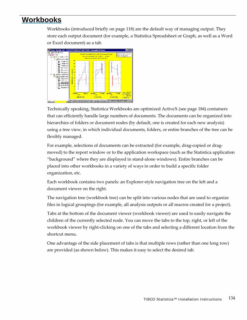
134 TIBCO Statistica™ Installation Instructions
Workbooks Workbooks (introduced briefly on page 118) are the default way of managing output. They store each output document (for example, a Statistica Spreadsheet or Graph, as well as a Word or Excel document) as a tab.
Technically speaking, Statistica Workbooks are optimized ActiveX (see page 184) containers that can efficiently handle large numbers of documents. The documents can be organized into hierarchies of folders or document nodes (by default, one is created for each new analysis) using a tree view, in which individual documents, folders, or entire branches of the tree can be flexibly managed.
For example, selections of documents can be extracted (for example, drag-copied or drag- moved) to the report window or to the application workspace (such as the Statistica application “background” where they are displayed in stand-alone windows). Entire branches can be placed into other workbooks in a variety of ways in order to build a specific folder organization, etc.
Each workbook contains two panels: an Explorer-style navigation tree on the left and a document viewer on the right.
The navigation tree (workbook tree) can be split into various nodes that are used to organize files in logical groupings (for example, all analysis outputs or all macros created for a project).
Tabs at the bottom of the document viewer (workbook viewer) are used to easily navigate the children of the currently selected node. You can move the tabs to the top, right, or left of the workbook viewer by right-clicking on one of the tabs and selecting a different location from the shortcut menu.
One advantage of the side placement of tabs is that multiple rows (rather than one long row) are provided (as shown below). This makes it easy to select the desired tab.
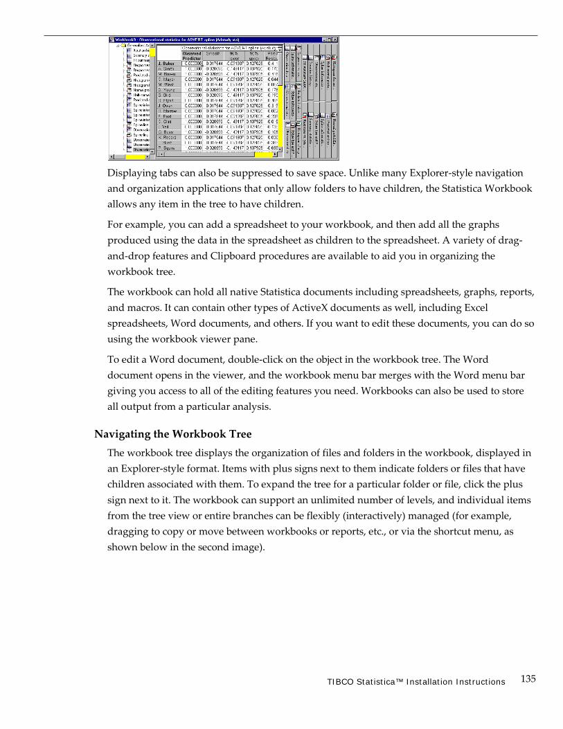
135 TIBCO Statistica™ Installation Instructions
Displaying tabs can also be suppressed to save space. Unlike many Explorer-style navigation and organization applications that only allow folders to have children, the Statistica Workbook allows any item in the tree to have children.
For example, you can add a spreadsheet to your workbook, and then add all the graphs produced using the data in the spreadsheet as children to the spreadsheet. A variety of drag- and-drop features and Clipboard procedures are available to aid you in organizing the workbook tree.
The workbook can hold all native Statistica documents including spreadsheets, graphs, reports, and macros. It can contain other types of ActiveX documents as well, including Excel spreadsheets, Word documents, and others. If you want to edit these documents, you can do so using the workbook viewer pane.
To edit a Word document, double-click on the object in the workbook tree. The Word document opens in the viewer, and the workbook menu bar merges with the Word menu bar giving you access to all of the editing features you need. Workbooks can also be used to store all output from a particular analysis.
Navigating the Workbook Tree The workbook tree displays the organization of files and folders in the workbook, displayed in an Explorer-style format. Items with plus signs next to them indicate folders or files that have children associated with them. To expand the tree for a particular folder or file, click the plus sign next to it. The workbook can support an unlimited number of levels, and individual items from the tree view or entire branches can be flexibly (interactively) managed (for example, dragging to copy or move between workbooks or reports, etc., or via the shortcut menu, as shown below in the second image).

136 TIBCO Statistica™ Installation Instructions
To select a workbook item for review or editing, simply locate the file in the workbook tree and click on its associated icon. The document will be displayed in the workbook viewer pane.
You can also navigate through the children of the currently selected node using the navigation tabs available (by default) at the bottom of the workbook viewer. You can easily move these navigation tabs to the top, right, or left of the workbook viewer by right-clicking on one of the tabs and selecting a different location from the shortcut menu or selecting the appropriate command from the Workbook tab, Tools group, Tab Control menu. Note that tabs at the top and bottom of the viewer scroll sideways, while multiple rows of tabs are used when tabs are placed to the left or right of the viewer.
Items in the tree are identified by the icon next to them. The folder icon represents a folder that can contain a variety of documents and subfolders. The folder icon with a red arrow on it indicates that the script that produced the results in that folder has been attached to the folder.
This enables Statistica to rerun or resume the analysis (for more details, see Chapter 8 – Statistica Visual Basic). The spreadsheet, report, macro, and graph icons represent Statistica Spreadsheet, Report, Macro, and Graph documents, respectively. The Data Miner icon represents a Data Miner workspace.
All non-Statistica documents are represented by their respective document icons. For example, Word documents are represented by the Word icon, and Excel spreadsheet files are represented by the Excel spreadsheet icon.
Commands for inserting, extracting, renaming, and removing items from the workbook tree are available from the workbook tree shortcut menu (accessed by right-clicking anywhere in the tree).
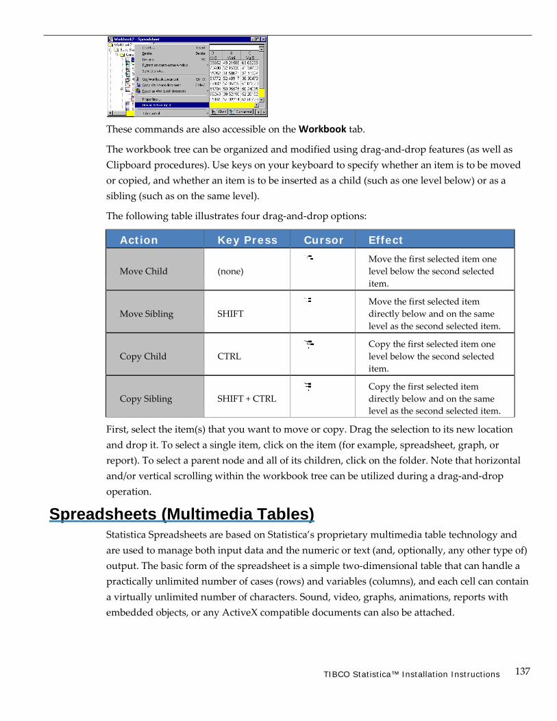
137 TIBCO Statistica™ Installation Instructions
These commands are also accessible on the Workbook tab.
The workbook tree can be organized and modified using drag-and-drop features (as well as Clipboard procedures). Use keys on your keyboard to specify whether an item is to be moved or copied, and whether an item is to be inserted as a child (such as one level below) or as a sibling (such as on the same level).
The following table illustrates four drag-and-drop options:
Action Key Press Cursor Effect
Move Child
(none)
Move the first selected item one
level below the second selected item.
Move Sibling
SHIFT
Move the first selected item
directly below and on the same level as the second selected item.
Copy Child
CTRL
Copy the first selected item one
level below the second selected item.
Copy Sibling
SHIFT + CTRL
Copy the first selected item
directly below and on the same level as the second selected item.
First, select the item(s) that you want to move or copy. Drag the selection to its new location and drop it. To select a single item, click on the item (for example, spreadsheet, graph, or report). To select a parent node and all of its children, click on the folder. Note that horizontal and/or vertical scrolling within the workbook tree can be utilized during a drag-and-drop operation.
Spreadsheets (Multimedia Tables) Statistica Spreadsheets are based on Statistica’s proprietary multimedia table technology and are used to manage both input data and the numeric or text (and, optionally, any other type of) output. The basic form of the spreadsheet is a simple two-dimensional table that can handle a practically unlimited number of cases (rows) and variables (columns), and each cell can contain a virtually unlimited number of characters. Sound, video, graphs, animations, reports with embedded objects, or any ActiveX compatible documents can also be attached.

138 TIBCO Statistica™ Installation Instructions
Because Statistica Spreadsheets can also contain macros and any user-defined user interface, these multimedia tables can be used as a framework for custom applications (for example, with a list box of options or a series of buttons placed in the upper-left corner), self-running presentations, animations, simulations, etc.
Data file layout in spreadsheets. Statistica data are organized into cases and variables. If you are unfamiliar with this notation, you can think of cases as the equivalent of records in a database management program (or rows of a spreadsheet), and variables as the equivalent of fields (or columns of a spreadsheet). Each case consists of a set of values of variables, and the first column in the file can (optionally) contain names of cases.
The spreadsheet window comprises several basic components.
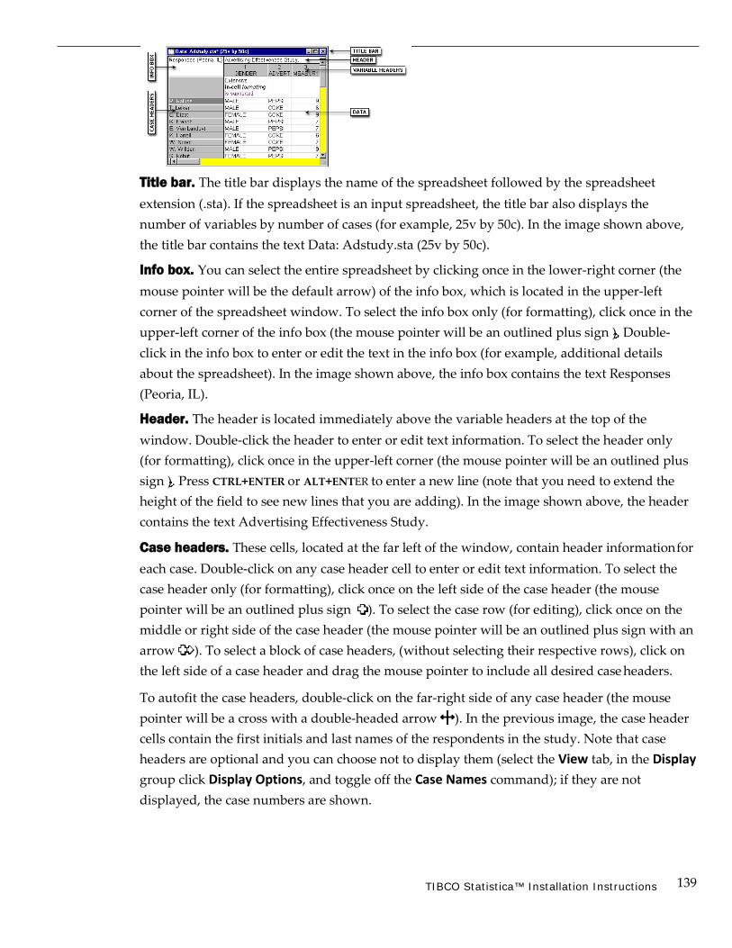
139 TIBCO Statistica™ Installation Instructions
Title bar. The title bar displays the name of the spreadsheet followed by the spreadsheet extension (.sta). If the spreadsheet is an input spreadsheet, the title bar also displays the number of variables by number of cases (for example, 25v by 50c). In the image shown above, the title bar contains the text Data: Adstudy.sta (25v by 50c).
Info box. You can select the entire spreadsheet by clicking once in the lower-right corner (the mouse pointer will be the default arrow) of the info box, which is located in the upper-left corner of the spreadsheet window. To select the info box only (for formatting), click once in the upper-left corner of the info box (the mouse pointer will be an outlined plus sign ). Double- click in the info box to enter or edit the text in the info box (for example, additional details about the spreadsheet). In the image shown above, the info box contains the text Responses (Peoria, IL).
Header. The header is located immediately above the variable headers at the top of the window. Double-click the header to enter or edit text information. To select the header only (for formatting), click once in the upper-left corner (the mouse pointer will be an outlined plus sign ). Press CTRL+ENTER or ALT+ENTER to enter a new line (note that you need to extend the height of the field to see new lines that you are adding). In the image shown above, the header contains the text Advertising Effectiveness Study.
Case headers. These cells, located at the far left of the window, contain header information for each case. Double-click on any case header cell to enter or edit text information. To select the case header only (for formatting), click once on the left side of the case header (the mouse pointer will be an outlined plus sign ). To select the case row (for editing), click once on the middle or right side of the case header (the mouse pointer will be an outlined plus sign with an arrow ). To select a block of case headers, (without selecting their respective rows), click on the left side of a case header and drag the mouse pointer to include all desired case headers.
To autofit the case headers, double-click on the far-right side of any case header (the mouse pointer will be a cross with a double-headed arrow ). In the previous image, the case header cells contain the first initials and last names of the respondents in the study. Note that case headers are optional and you can choose not to display them (select the View tab, in the Display group click Display Options, and toggle off the Case Names command); if they are not displayed, the case numbers are shown.

140 TIBCO Statistica™ Installation Instructions
Variable headers. These cells, located at the top of each column, contain header information for each variable. To display details about an individual variable, double-click on the variable header cell.
To select the variable header only (for formatting) click once in the upper portion of the variable header (the mouse pointer will be an outlined plus sign ). To select the variable column (for editing) click once in the lower portion of the variable header (the mouse pointer will be an outlined plus sign with an arrow ).
To autofit the variable column, double-click on the right side of the variable header (the mouse pointer will be a cross with a double-headed arrow ). In the previous image, the first two variable header cells contain the text GENDER and ADVERT. You have the option to change how the variable header cells display information so that they show the column number associated with the variable, the variable long name, and/or an abbreviation of the display types for the variables in the spreadsheet. Each of these options is available on the View tab in the Display group; click Variable Headers.
Data (and in-cell formatting options). The remainder of the spreadsheet contains data that pertain to the cases and variables and any optional attached or linked objects (multimedia objects, macros, custom user interface). Text in cells can be of practically unlimited length (in most Statistica configurations it is limited to 1,000 characters to protect against inadvertent pasting of unwanted large amounts of data into one cell). Text in cells can be extensively formatted including wrapping the text, different fonts, and font attributes.
Input vs. Output Spreadsheets Statistica offers the ability to open and use many spreadsheets at the same time, allowing you to work with several different input data files simultaneously. In addition to storing data, Statistica uses spreadsheets to display the numeric output from its analyses. Because Statistica makes no distinction in the features supported for an input spreadsheet (from which Statistica retrieves its data) and an output spreadsheet (where the results of an analysis are displayed), it is easy to use the results of one analysis as input data for further analyses.
Any spreadsheet opened from a disk file is automatically treated as an input spreadsheet, and any number of input spreadsheets can be open at a time. To avoid confusion, however, an output spreadsheet (containing the results of an analysis) is not automatically available as input data for analysis. It must first be designated as an input spreadsheet before being used for further analyses. Additionally, input spreadsheets report the number of variables and cases for that spreadsheet in the title bar. For example, if Exp.sta (88v by 48c) is in the title bar, it is an input spreadsheet; if Exp.sta is in the title bar, it is not an input spreadsheet.

141 TIBCO Statistica™ Installation Instructions
To designate an output spreadsheet as an input spreadsheet, select the spreadsheet (such as ensure the spreadsheet has the focus). Then, on the Data tab in the Mode group, select the Input check box. Now you can begin an analysis, and Statistica will use the data from the specified input spreadsheet for the analysis. Note that if you switch back to another spreadsheet that has previously been designated as an input spreadsheet, it can still be used for analyses as well.
In a workbook, only one spreadsheet can be selected for analyses at a time, even if the workbook contains several input spreadsheets. This spreadsheet is called the Active Input spreadsheet, and its icon (in the workbook tree) is framed in red.
By default, when an output spreadsheet is designated as an input spreadsheet, Statistica automatically selects it as the Active Input spreadsheet. To select another input spreadsheet for active input, select the Active Input check box on the Workbook tab in the Items group, or select Use as Active Input from the workbook tree shortcut menu.
It is also possible to leave a stand-alone spreadsheet open but designate it as unavailable for analysis. To do this, select the spreadsheet, and clear the Input check box on the Data tab in the Mode group. Now Statistica automatically defaults to the most recently selected input spreadsheet for analysis, ignoring all spreadsheets that are not designated as input spreadsheets.
Statistica Spreadsheet OLE DB Provider In addition to using spreadsheets as data sources for analyses in Statistica, spreadsheets can also supply data to other database-aware applications by using the Statistica OLE DB Provider for Statistica Spreadsheets. This OLE DB driver is installed with Statistica, and allows read- only access to data in Statistica Spreadsheets using the industry-standard Structured Query Language (SQL). You can access the OLE DB Provider at any point the system allows you to choose a database connection, using the standard Microsoft Data Link Properties.

142 TIBCO Statistica™ Installation Instructions
To access this functionality, select the Data tab. In the Manage group, click External Data and from the drop-down list, select Create Query. In the Database Connection dialog, click the New button to display the Data Link Properties dialog, where you select Statistica OLE DB Provider for Statistica Spreadsheets.
Click the Next button to display the Connection tab.
The Data Source field specifies the directory path where the spreadsheet is located. When creating the query, you can choose individual spreadsheet files within that directory. The following example uses Statistica Query, and has defined a connection to the Spreadsheet OLE DB, specifying the path of the Statistica Examples folder. Each spreadsheet within the folder shows up as a potential table.
These spreadsheets can be referenced in FROM clauses, specific variable names selected as fields in SELECT clauses, and cases defined with WHERE clauses. Joins between multiple spreadsheets are supported as well, using standard JOIN clauses.

143 TIBCO Statistica™ Installation Instructions
Using the StatSoft OLE DB Provider for Statistica Spreadsheets enables you to provide Statistica Spreadsheet data to any application (including Statistica itself) that can use the industry-standard OLE DB interface for querying data.
Reports Reports (briefly introduced on page 119) in Statistica offer a more traditional way of handling output (compared to workbooks) as each object (for example, a Statistica Spreadsheet or Graph, or an Excel spreadsheet) is displayed sequentially in a word processor style document.
However, the technology behind this simple report offers you rich functionality. For example, like the workbook, each Statistica Report is also an ActiveX (see page 184) container where each of its objects (not only Statistica Spreadsheets and Graphs, but also any other ActiveX- compatible documents, for example, Word documents) is active, customizable, and in-place editable. Reports are stored in the STR file format, which is a Statistica extension of the Microsoft RTF (Rich Text Format, *.rtf) format. STR files share the RTF formatting information and additionally they include the tree view information (which cannot be stored in the standard RTF files). Report files are by default saved with the file name extension *.str, but they can also be saved as standard RTF files (in which case the tree information will not be preserved).
144 TIBCO Statistica™ Installation Instructions
The obvious advantages of this way of handling output (more traditional than the workbook) are the ability to insert notes and comments “in between” the objects as well as its support for the more traditional way of quickly scrolling through and reviewing the output to which some users may be accustomed.
Also, only the report output includes and preserves a record of the supplementary information, which contains a detailed log of the options specified for the analyses (for example, selected variables and their labels, long names, etc., depending on the level of supplementary information specified in the Output Manager, see page 21).
The obvious drawback, however, of these traditional reports is the inherent flat structure imposed by their word processor style format, though that is what some users of certain applications may favor.
Navigating the Report Tree The report tree displays the organization of files in the report. The files are displayed in an Explorer-style format; however, unlike workbooks that can support any number of levels, the report supports only one level of files.
You can embed any type of Statistica document in a report, including spreadsheets, graphs, and analyses. In addition to Statistica document types, you can embed other types of ActiveX/OLE objects in a report, including Excel spreadsheets, Word documents, bitmap images, and others.
To edit one of these types of embedded documents, double-click on the document. The file opens in the viewer, and the report toolbar merges with the toolbar from the embedded file’s native application, giving you access to all of the editing features you need.
Items in the tree are identified by the icon next to them. The spreadsheet, macro, and graph icons represent Statistica Spreadsheet, Macro, and Graph documents, respectively. The
Data Miner icon represents a Data Miner workspace. All non-Statistica documents are represented by their document icons. For example, Word documents are represented by the Word icon, and Excel spreadsheet files are represented by the Excel spreadsheet icon.
The report tree can be organized and modified using drag-and-drop features as well as Clipboard procedures.
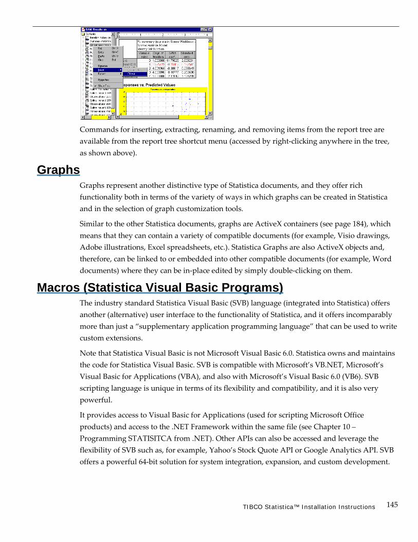
145 TIBCO Statistica™ Installation Instructions
Commands for inserting, extracting, renaming, and removing items from the report tree are available from the report tree shortcut menu (accessed by right-clicking anywhere in the tree, as shown above).
Graphs Graphs represent another distinctive type of Statistica documents, and they offer rich functionality both in terms of the variety of ways in which graphs can be created in Statistica and in the selection of graph customization tools.
Similar to the other Statistica documents, graphs are ActiveX containers (see page 184), which means that they can contain a variety of compatible documents (for example, Visio drawings, Adobe illustrations, Excel spreadsheets, etc.). Statistica Graphs are also ActiveX objects and, therefore, can be linked to or embedded into other compatible documents (for example, Word documents) where they can be in-place edited by simply double-clicking on them.
Macros (Statistica Visual Basic Programs) The industry standard Statistica Visual Basic (SVB) language (integrated into Statistica) offers another (alternative) user interface to the functionality of Statistica, and it offers incomparably more than just a “supplementary application programming language” that can be used to write custom extensions.
Note that Statistica Visual Basic is not Microsoft Visual Basic 6.0. Statistica owns and maintains the code for Statistica Visual Basic. SVB is compatible with Microsoft’s VB.NET, Microsoft’s Visual Basic for Applications (VBA), and also with Microsoft’s Visual Basic 6.0 (VB6). SVB scripting language is unique in terms of its flexibility and compatibility, and it is also very powerful.
It provides access to Visual Basic for Applications (used for scripting Microsoft Office products) and access to the .NET Framework within the same file (see Chapter 10 – Programming STATISITCA from .NET). Other APIs can also be accessed and leverage the flexibility of SVB such as, for example, Yahoo’s Stock Quote API or Google Analytics API. SVB offers a powerful 64-bit solution for system integration, expansion, and custom development.

146 TIBCO Statistica™ Installation Instructions
Statistica Visual Basic takes full advantage of the object model architecture of Statistica and is used to access programmatically every aspect and virtually every detail of the functionality of Statistica. Even the most complex analyses and graphs can be recorded into Visual Basic macros and later be run repeatedly or edited and used as building blocks of other applications. Statistica Visual Basic adds an arsenal of more than 14,000 new functions to the standard comprehensive syntax of Visual Basic, thus comprising one of the largest and richest development environments available.
Statistica Macros can be saved in several formats, depending on how you intend to use them. You can also copy them to the Clipboard and paste them into other programs or documents.
Statistica Visual Basic is discussed in more detail in Chapter 8.
Statistica Projects When performing statistical analyses and working with Statistica documents, you will often have many different windows open, and even different analyses in different stages of progress. Statistica provides a means for saving your workspace, including any analyses in progress. You can close Statistica at any point during an analysis, and when you later re-open the project, the previously opened files and in-process analyses will be restored.
To save a Statistica Project, select the Home tab, click the Save arrow in the Project group, and select Save Project As to display the Save Statistica Project dialog.

147 TIBCO Statistica™ Installation Instructions
In this dialog, specify the path and file name of the Statistica Project file (a project’s extension is .spf). You can also specify what items to include in the project. All Statistica document types can be selected (Spreadsheets, Graphs, Workbooks, Macros, Reports, Data Miner projects, In- Place Database projects, Analyses, and Analysis results). For those Statistica documents that are already stored on disk, you have the option to either Link to the existing document file, or to store a copy of the document within the Statistica Project file (Embed the document in the project).
In addition to Statistica documents, project files will also save all in-progress analyses. The project file will store the recorded scripts that are automatically created when every analysis is run. When the project is re-opened, the scripts for the analyses are re-run against the original data and the analyses dialogs are made visible again in exactly the state they were when the project file was saved.
Project files are a convenient way to send in-progress analysis steps and results back and forth between users if you elect to embed the saved documents in the project file. One user can run analyses to a certain point, and then save the project file and pass it to another user, who can open the project file and continue exactly where the first user stopped the analyses.
Unless you configure it otherwise, Statistica will automatically display a prompt asking if you want to save a project file when quitting the program, and will automatically re-open the last- saved project file when starting. Thus, Statistica makes it easy to quit for the day and start the next session right where you left off.
Note that a project is a state of an instance of Statistica. Thus, projects are not like other documents in that you cannot open more than one project in a single instance of Statistica. A different (second) project can be opened in a second instance of Statistica.

148 TIBCO Statistica™ Installation Instructions
Chapter Six Graphs
149 TIBCO Statistica™ Installation Instructions
Overview The most common application of graphs is to efficiently present and communicate information (typically, numerical data). However, graphical techniques also provide powerful analytical tools for the exploration of data and verification of hypotheses.
A broad selection of graphics options. Statistica includes a comprehensive selection of graphical methods for both data analysis and the presentation of results. All graphs in Statistica include a broad selection of built-in, interactive analytic techniques and extensive customization tools that enable you to interactively control virtually all aspects of the display.
Also, flexible graphics management facilities are available that are used to integrate various graphical displays and to build dynamic links between applications (for example, using OLE- Object Linking and Embedding).
Comprehensive support for Visual Basic and other languages. Statistica graphical options can also be accessed programmatically (using built-in Statistica Visual Basic or other compatible languages), which creates practically unlimited possibilities for producing highly customized graphical displays.
These custom graphs can later be permanently added to Statistica’s user interface (for example, assigned to buttons on toolbars or added to the menus).
General categories of graphs. The Statistica system offers a variety of methods in which graphs can be requested or defined.
They complement each other, providing a high level of integration between numbers (such as raw data, intermediate results, or final results) and graphical displays. For example, specialized graphs can be requested as part of the automatic output from statistical procedures, but they can also be requested via integrated tools to visualize virtually any combination of numbers (and/or labels) that are displayed or generated by Statistica.
Customization of Graphs Interactive graph customization. The customization options in Statistica graphics include hundreds of features and tools that can be used to adjust every detail of the display and associated data processing. However, these options are arranged in a hierarchical manner, so those used most often are accessible directly via shortcuts by double-clicking or right-clicking on the respective element of the graph.
Permanent settings and automation options. The initial (default) settings of all of these features can be easily adjusted so that even the default appearance and behavior of Statistica graphs will match your specific needs and/or will require very little intervention on your part. Following are some of the ways to make these adjustments:

150 TIBCO Statistica™ Installation Instructions
1. Options dialog. Perhaps the most straightforward way to adjust the default appearance of graphs is by modifying the graph options in the Options dialog (select the Tools tab and click Options). Most commonly used settings can be easily adjusted there (select Display or Settings, located under Graphs), and the results will be reflected in the default styles (see number 2 below) that will be used by the system and as such, they will be automatically saved in the Statistica configuration file (for example, different settings can be used for different projects).
2. Graph style system. All of the numerous features that affect the appearance of the graph (from as elementary as the color of the font in the footnote to as general as the global features of the graph document) can be saved as individual “styles.” These styles can be given custom names and later be reapplied using simple shortcuts (such as pressing a specific key combination or clicking a button on a custom toolbar). An intelligent system internally manages these thousands of styles and their combinations in Statistica and helps you achieve your customization objectives with a minimum amount of effort. All user-defined or modified styles will be saved automatically in the Statistica configuration file (for example, different sets or systems of styles can be used for different projects).
3. User-defined graphs. New types of graphs can be defined in a variety of ways and can be added to the menus, dialogs, or toolbars. If a custom graph that you intend to use repeatedly is not built from scratch but is based on one of the Graphs menu graphs and is produced by some combination of the existing graph customization options, then adding it to the Graphs menu as a new type of graph is as simple as clicking the Add As User-defined Graph to Menu button on the Options 2 tab of the graph specification dialog. All user-defined graph specifications will be saved automatically in the Statistica configuration file (for example, different sets of custom graphs can be used for different projects).
4. Statistica Visual Basic. Finally, note that there are no limits to how “deeply customized” your Statistica custom graphs can be, because Statistica Visual Basic (with all its powerful custom drawing tools as well as the Statistica-based library of graphics procedures) can be used to produce virtually any graphics or multimedia output supported by the contemporary computer hardware. Those custom developed displays or multimedia output can be assigned to Statistica toolbars, menus, or dialogs and become a permanent part of “your” Statistica application.
The default settings of most graphs offered in Statistica follow the established conventions that are either explicitly described in the literature on statistical and technical graphing, or they represent standards that are commonly accepted by major scientific journals (for example, SCIENCE). However, practically all default settings of Statistica can be customized to meet specific requirements of unusual applications (see page 149). Statistica’s graphics facilities were designed to play the role of flexible tools, capable of producing effects that go far beyond established patterns and templates.

151 TIBCO Statistica™ Installation Instructions
In addition to a comprehensive selection of standard statistical and technical graphs, Statistica includes numerous unique types of graphs and graph customization facilities. The Graph Options dialog, accessible by double-clicking in the background of a graph, or selecting the Tools tab and clicking Graph in the Options group, contains options that address all of the relevant customizable features for a particular graph. The options are grouped in clusters containing logically related items, and are an all-inclusive “superset” of graph shortcut options accessed by double-clicking specific graph features.
Located at the bottom of graphs, you’ll find the interactive graphics controls (see the next illustrations), which enable you to adjust the transparency of the plot areas and markers, and to scroll and pan in order to interactively scale the graph. More controls are located in 3D graphs to enable interactive rotation. Click the wrench icon adjacent to the sliders to display the Graph Options dialog.
Left: 2D Graph
Below: Enlarged image of Panning (scaling), Scrolling, and Transparency Controls

152 TIBCO Statistica™ Installation Instructions
Left: Plot Area Transparency Control circled; making plot areas transparent allows portions of the plot to overlap while still being visible
Left: 3D Graph; Rotation Controls circled
Below: Enlarged image of Rotation and Transparency Controls
While Statistica statisticians designed most of the graph customization options, it is important to say that Statistica users have played a significant role in their creation. In fact, the selection of graphics options included in Statistica is the result of input from thousands of users who provided their comments in response to Statistica’s inquiries. Many unique facilities of Statistica Graphs were introduced in response to users’ ideas and requests. We at Statistica are very grateful for the input from our users.
As mentioned previously (and discussed in detail on page 156), there are various methods to specify Statistica Graphs. You could say that these methods represent different types of interfaces between numbers and graphs.
For example, the numbers represented in a pie chart can simply depict values of a spreadsheet column (for example, variable Sales) in the consecutive cases of the spreadsheet (for example, cases labeled: Year 2008, Year 2009, Year 2010, ..., etc.).

153 TIBCO Statistica™ Installation Instructions
The numbers in a similar pie chart, however, can represent results of calculations. For example, the slices of the pie can represent relative frequencies of observations that belong to certain categories calculated by one of the histogram or frequency categorization procedures (for example, numbers of years when the Sales were below $10 million, between $10 and $20 million, and above $20 million).
Regardless of the method that was used to create a graph (such as regardless of where the numbers represented in the graph were obtained or how they were calculated), all Statistica Graph customization and multigraphics management facilities can be used to change the appearance of the graph or integrate it with other graphs or documents.

154 TIBCO Statistica™ Installation Instructions
Also, all integrated analytic facilities that are accessible from within graphs in Statistica (such as function fitting, smoothing, rotation, brushing, analytical zooming, etc.) are available and can be applied to the graph regardless of the source of the numbers in the graph or the method that was used to create it.
The graph editing facilities offered in Statistica enable you to create not only highly customized scientific and technical publication-ready displays:
and precise drawings:

155 TIBCO Statistica™ Installation Instructions
but also presentation-quality diagrams, posters, business charts, and other displays:
that are designed to communicate information in an effective and attractive manner.
Graphs that are saved into files or that in any other way have been temporarily detached from the Statistica application (for example, copied to the Clipboard or linked to a document in another application) are complete “objects” (technically speaking, ActiveX objects, see page 184) that contain not only all customization features and other embedded objects, but also all data that are necessary to continue editing all aspects of the display or the analysis of its contents (fitting, smoothing, etc.).
156 TIBCO Statistica™ Installation Instructions
Because Statistica Graphs are ActiveX objects, they can easily be linked to or embedded in other compatible documents (for example, Excel or Word documents), where they can be in-place edited by double-clicking on them. Statistica Graphs are also ActiveX containers and, therefore, can contain a wide variety of embedded or linked documents such as Visio drawings, Adobe illustrations, Excel spreadsheets, or Word documents. Moreover, Statistica supports hierarchies of embedded objects up to four levels, which means that it can manage “documents containing documents, containing documents, which contain documents.”
General Categories of Graphs In addition to the specialized statistical graphs that are available from the output dialogs in all statistical procedures (see page 163), there are two general categories or classes of graphs both accessible from the Graphs tab, shortcut menus, and the Statistica Start button menu:
• Input data graphs (Graphs of Input Data, see page 157) and Graphs menu graphs, (see page 160) and
• Graphs of Block Data (see page 158).
The most important difference between these two general categories lies in the data that the graph types utilize for generating plots.
Input data graphs. Graphs of Input Data and their expanded version on the Graphs tab produce statistical summaries or other representations of the raw data in the current input data spreadsheet (typically for all the variables, or for subsets if case selection conditions are used).
If graphs of this general category are produced using a shortcut menu from within a spreadsheet of results that does not contain the actual data (for example, a correlation matrix), Statistica will still reach to the respective input (raw) data to produce the graph (for example, a scatterplot of the variables identified by the selected cell in the correlation matrix from which the shortcut menu was opened).
Graphs of Block Data. Graphs of Block Data, however, are entirely independent of the concept of input data or data file. They provide a general tool to visualize numeric values in the currently selected block of any spreadsheet (which can contain values from custom defined subsets of numerical output or arbitrarily selected subsets of raw data).
Common features of the two categories of graphs. These two general categories of graphs offer the same customization options and the same selection of types of graphs. For example, you can create the same highly specialized categorized ternary graph from the input (raw) data set and from a custom defined block of values representing results of a particular test.
These two general categories of graphs will be briefly discussed in the next two sections, followed by a section on the Graphs tab, which contains an exhaustive selection of all graphs from the first category (input data graphs, often referred to as Graphs menu graphs), as well as access to Graphs of Block Data and other options.
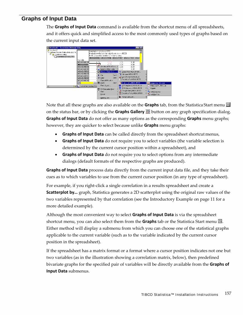
157 TIBCO Statistica™ Installation Instructions
Graphs of Input Data The Graphs of Input Data command is available from the shortcut menu of all spreadsheets, and it offers quick and simplified access to the most commonly used types of graphs based on the current input data set.
Note that all these graphs are also available on the Graphs tab, from the Statistica Start menu on the status bar, or by clicking the Graphs Gallery button on any graph specification dialog. Graphs of Input Data do not offer as many options as the corresponding Graphs menu graphs; however, they are quicker to select because unlike Graphs menu graphs:
• Graphs of Input Data can be called directly from the spreadsheet shortcut menus, • Graphs of Input Data do not require you to select variables (the variable selection is
determined by the current cursor position within a spreadsheet), and • Graphs of Input Data do not require you to select options from any intermediate
dialogs (default formats of the respective graphs are produced).
Graphs of Input Data process data directly from the current input data file, and they take their cues as to which variables to use from the current cursor position (in any type of spreadsheet).
For example, if you right-click a single correlation in a results spreadsheet and create a Scatterplot by… graph, Statistica generates a 2D scatterplot using the original raw values of the two variables represented by that correlation (see the Introductory Example on page 11 for a more detailed example).
Although the most convenient way to select Graphs of Input Data is via the spreadsheet shortcut menu, you can also select them from the Graphs tab or the Statistica Start menu . Either method will display a submenu from which you can choose one of the statistical graphs applicable to the current variable (such as to the variable indicated by the current cursor position in the spreadsheet).
If the spreadsheet has a matrix format or a format where a cursor position indicates not one but two variables (as in the illustration showing a correlation matrix, below), then predefined bivariate graphs for the specified pair of variables will be directly available from the Graphs of Input Data submenus.

158 TIBCO Statistica™ Installation Instructions
Otherwise, such as when the current cursor position indicates only one variable as in a table of descriptive statistics (as shown in the next illustration), and if you select any of the bivariate graphs in the menu, Statistica will prompt you to select the second variable. For example, if you select Scatterplot by, the Select second variable dialog will be displayed, where you specify by which variable Measure05 is going to be plotted.
If more than one variable is indicated by a highlighted section (such as when a block is selected), then the Graphs of Input Data menu will apply to the first selected variable.
When generating Graphs of Input Data, Statistica takes into account the current case selection and weighting conditions for the variables that are being plotted. Note, however, that the case selection or weighting conditions need to be specified for the current spreadsheet (such as via the Tools tab Selection Conditions - Edit options and the Tools tab Weight options) and not just “locally” for an analysis (such as selected from the respective analysis/graph specification dialogs using the and buttons). The latter conditions will be ignored by the Graphs of Input Data.
Graphs of Block Data Unlike Graphs of Input Data, Graphs of Block Data use the currently selected (continuous) block of data in the active spreadsheet to specify input data for the graph.
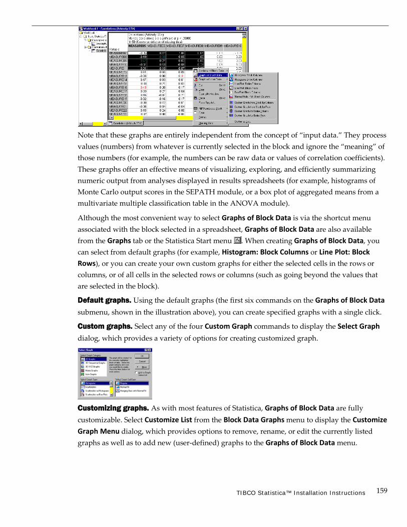
159 TIBCO Statistica™ Installation Instructions
Note that these graphs are entirely independent from the concept of “input data.” They process values (numbers) from whatever is currently selected in the block and ignore the “meaning” of those numbers (for example, the numbers can be raw data or values of correlation coefficients). These graphs offer an effective means of visualizing, exploring, and efficiently summarizing numeric output from analyses displayed in results spreadsheets (for example, histograms of Monte Carlo output scores in the SEPATH module, or a box plot of aggregated means from a multivariate multiple classification table in the ANOVA module).
Although the most convenient way to select Graphs of Block Data is via the shortcut menu associated with the block selected in a spreadsheet, Graphs of Block Data are also available from the Graphs tab or the Statistica Start menu . When creating Graphs of Block Data, you can select from default graphs (for example, Histogram: Block Columns or Line Plot: Block Rows), or you can create your own custom graphs for either the selected cells in the rows or columns, or of all cells in the selected rows or columns (such as going beyond the values that are selected in the block).
Default graphs. Using the default graphs (the first six commands on the Graphs of Block Data submenu, shown in the illustration above), you can create specified graphs with a single click.
Custom graphs. Select any of the four Custom Graph commands to display the Select Graph dialog, which provides a variety of options for creating customized graph.
Customizing graphs. As with most features of Statistica, Graphs of Block Data are fully customizable. Select Customize List from the Block Data Graphs menu to display the Customize Graph Menu dialog, which provides options to remove, rename, or edit the currently listed graphs as well as to add new (user-defined) graphs to the Graphs of Block Data menu.
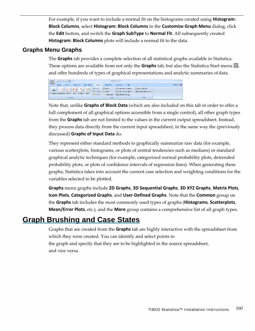
160 TIBCO Statistica™ Installation Instructions
For example, if you want to include a normal fit on the histograms created using Histogram: Block Columns, select Histogram: Block Columns in the Customize Graph Menu dialog, click the Edit button, and switch the Graph SubType to Normal Fit. All subsequently created Histogram: Block Columns plots will include a normal fit to the data.
Graphs Menu Graphs The Graphs tab provides a complete selection of all statistical graphs available in Statistica. These options are available from not only the Graphs tab, but also the Statistica Start menu , and offer hundreds of types of graphical representations and analytic summaries of data.
Note that, unlike Graphs of Block Data (which are also included on this tab in order to offer a full complement of all graphical options accessible from a single control), all other graph types from the Graphs tab are not limited to the values in the current output spreadsheet. Instead, they process data directly from the current input spreadsheet, in the same way the (previously discussed) Graphs of Input Data do.
They represent either standard methods to graphically summarize raw data (for example, various scatterplots, histograms, or plots of central tendencies such as medians) or standard graphical analytic techniques (for example, categorized normal probability plots, detrended probability plots, or plots of confidence intervals of regression lines). When generating these graphs, Statistica takes into account the current case selection and weighting conditions for the variables selected to be plotted.
Graphs menu graphs include 2D Graphs, 3D Sequential Graphs, 3D XYZ Graphs, Matrix Plots, Icon Plots, Categorized Graphs, and User-Defined Graphs. Note that the Common group on the Graphs tab includes the most commonly used types of graphs (Histograms, Scatterplots, Mean/Error Plots, etc.), and the More group contains a comprehensive list of all graph types.
Graph Brushing and Case States Graphs that are created from the Graphs tab are highly interactive with the spreadsheet from which they were created. You can identify and select points in the graph and specify that they are to be highlighted in the source spreadsheet, and vice versa.

161 TIBCO Statistica™ Installation Instructions
In addition to selecting points in graphs and spreadsheets, you can identify properties of a case in a spreadsheet that will be used when the graph is created from that data. These properties include the point marker style and color, and whether the point is to be excluded from the graph and/or fit calculations.
To start brushing within a graph, click the brushing button on the Edit tab in the Customize Graph group, or right-click in the background of a graph and select Show Brushing from the shortcut menu to display the Brushing dialog, which is shown in the illustration to the right.
With the default Selection Brush, which is Simple, you can draw a rectangle on the graph to select the points contained in the rectangle. The following illustration demonstrates this for the example data set Adstudy.sta, with a 2D scatterplot of MEASURE01 by MEASURE02.
Note that the upper-left three points have been selected by the brushing tool, which highlights the points in the graph as well as the corresponding cases in the spreadsheet from which the graph was created.
Alternatively, instead of using the Brushing facilities, you can select cases in the spreadsheet (click on the far-left side of the case name) and the corresponding points will be marked in the graph, as shown in the following illustration, where the first five cases in the Adstudy.sta spreadsheet have been selected.
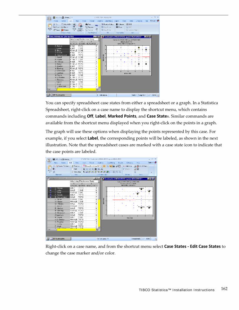
162 TIBCO Statistica™ Installation Instructions
You can specify spreadsheet case states from either a spreadsheet or a graph. In a Statistica Spreadsheet, right-click on a case name to display the shortcut menu, which contains commands including Off, Label, Marked Points, and Case States. Similar commands are available from the shortcut menu displayed when you right-click on the points in a graph.
The graph will use these options when displaying the points represented by this case. For example, if you select Label, the corresponding points will be labeled, as shown in the next illustration. Note that the spreadsheet cases are marked with a case state icon to indicate that the case points are labeled.
Right-click on a case name, and from the shortcut menu select Case States - Edit Case States to change the case marker and/or color.

163 TIBCO Statistica™ Installation Instructions
Note that the selection of points is available for graph types other than Scatterplots. For histograms, brushing/selecting a histogram bar will select the corresponding points to that bar in the spreadsheet. The same is true of the boxes in box plots.
Using case states and brushing and selecting points is particularly useful with the Hidden and Excluded case states options. First, to make these options available, display the Options dialog (select the Tools tab and click Options), and in the tree view select Navigation / Defaults (located under Spreadsheets). Clear the Combine Excluded and Hidden Case States into Off state check box, and click the OK button.
Then, select the Data tab, and in the Cases group click Cases. From the Case States submenu, select Hidden to mark a case as hidden, such as the case will not be visible in graphs, but will be used in analyses. You can also right-click on a case name, and from the shortcut menu select Case States - Edit Case States to display the Case State dialog, where you can select the Hidden check box.
Select Excluded to mark a case as excluded, such as the case will not be used in the computations; however, the case will be displayed in most graph types. The case point marker is displayed, but the case is removed from computations. The Excluded case state also works in conjunction with spreadsheet selection conditions; any case that has the Excluded case state set will be treated as if the case were excluded by selection conditions. Therefore, using graph brushing and case states is a convenient tool to interactively remove outliers and then rerun analyses with the points removed.
When the Combine Excluded and Hidden Case States into Off state check box is selected in the Options dialog - Navigation / Defaults options pane, the Hidden and Excluded options are replaced with the Off option. Select Off to mark a case as Hidden and Excluded; the point will be excluded from computations and from graphs.
Other Specialized Graphs In addition to the standard selection of Graphs of Input Data, Graphs of Block Data, and Graphs menu graphs, other specialized statistical graphs that are related to a type of analysis (for example, cluster analysis results) are accessible directly from results dialogs (such as the dialogs that contain output options from the current analysis).
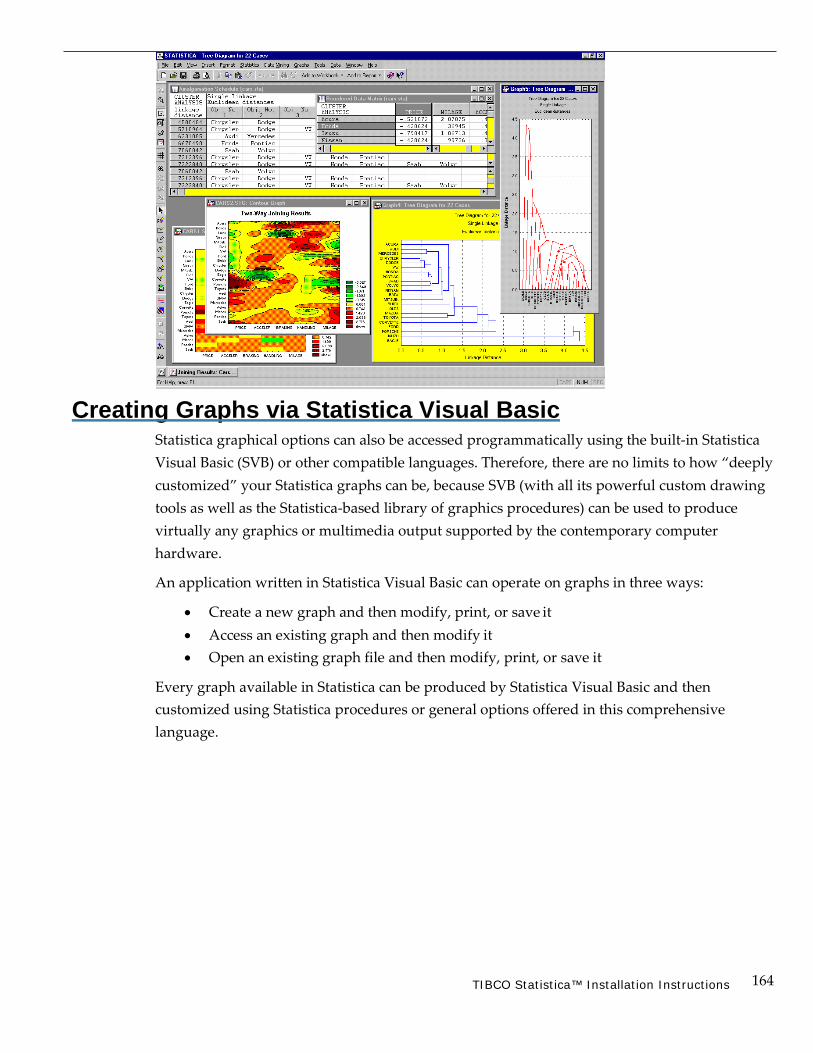
164 TIBCO Statistica™ Installation Instructions
Creating Graphs via Statistica Visual Basic Statistica graphical options can also be accessed programmatically using the built-in Statistica Visual Basic (SVB) or other compatible languages. Therefore, there are no limits to how “deeply customized” your Statistica graphs can be, because SVB (with all its powerful custom drawing tools as well as the Statistica-based library of graphics procedures) can be used to produce virtually any graphics or multimedia output supported by the contemporary computer hardware.
An application written in Statistica Visual Basic can operate on graphs in three ways:
• Create a new graph and then modify, print, or save it • Access an existing graph and then modify it • Open an existing graph file and then modify, print, or save it
Every graph available in Statistica can be produced by Statistica Visual Basic and then customized using Statistica procedures or general options offered in this comprehensive language.

165 TIBCO Statistica™ Installation Instructions
As with all other functions in Statistica Visual Basic, functions to access the graphics library of Statistica can be easily incorporated into Statistica Visual Basic programs via a hierarchically organized Function Browser. It contains short descriptions of all functions and options that can be inserted directly into the source code of your program (such as into the Statistica Visual Basic Editor, see page 175).

166 TIBCO Statistica™ Installation Instructions
Chapter Seven Customizing Statistica
167 TIBCO Statistica™ Installation Instructions
Customizing Statistica
Statistica offers the flexibility of fully customizable user interfaces and supports the necessary adjustment of the standard user interface to better suit your specific needs. In fact, Statistica anticipates your needs in that it remembers various choices as you make them. For example, if you launch an analysis from the Advanced tab on an analysis specification dialog, the Advanced tab will be selected (instead of the Quick tab) the next time you display that dialog.
Practically all aspects of the user interface can be customized starting with such elementary controls as the classic menus, Quick Access toolbar, and the keyboard. The process for customizing these screen components is quick and straightforward (for example, see the illustration of customizing the toolbar on page 111). You can set both global and local customizations for graphs, spreadsheets, workbooks, reports, etc., and maintain different configurations of Statistica (for a single user as well as for network users). You can also define entirely new user interfaces (see pages 111 and 112).
Customization of the Interactive User Interface As mentioned before, Statistica contains facilities to define entirely new user interfaces (see page 111), including the Internet browser-based user interfaces (see page 113). However, practically all aspects of the default, interactive user interface can also be adjusted easily in a variety of ways. For example, you can add to the default options, simplify them, or keep changing them as your needs change.
Depending on the requirements of the tasks to be performed, as well as your personal preferences for particular “modes” of work (and aesthetic choices), you can suppress all icons, toolbars, status bars, long menus, workbook facilities, drag-and-drop facilities, dynamic (automatic) links between graphs and data, 3D effects in tables, and 3D effects in dialog boxes; request “bare-bones” sequential output with simple, paper-white spreadsheets and monochrome graphs; and set the system to automatically maintain no more than one simple report at a time.
Or alternatively, you can define elaborate local and global toolbars; take full advantage of all special tools and controls, icons, toolbars, macros (for example, assign particular tasks to specific new classic menu commands, the Quick Access toolbar, or keys), elaborate multimedia tables, workbook facilities, and drag-and-drop facilities; establish multiple dynamic (automatic) links between graphs and data and internal links between graphical objects; customize the output windows with colors, special fonts, and highlights; adjust the default graph styles and their display modes; and send the results to separate hierarchically organized workbooks to create an elaborate, multi-layered data analysis environment that facilitates the exploration of complex data files and allows you to compare different aspects of the output.
168 TIBCO Statistica™ Installation Instructions
Customization of Documents There is a variety of comprehensive, specialized tools to customize the layout and operation of Statistica documents (see Chapter 5 – Statistica Documents). For example, Statistica has a comprehensive system of managing defaults of every aspect of graphs and combining customizations into hierarchically organized “styles.” Similarly, you can create custom layouts and formats for spreadsheets (multimedia tables) and even customize events (for example, what happens when you double-click on a table).
Local vs. Permanent Customizations Many aspects of the appearance of Statistica can be adjusted from both the View and Tools tabs. Each of these two methods, however, has a different function.
View tab. The changes specified on the View tab affect the current appearance of Statistica (for example, hides the Status Bar) or the current document window (for example, spreadsheet grid lines).
Options dialog. The options available in the Options dialog (select the Tools tab and click Options) are used to adjust the permanent program defaults (discussed in more detail in the next section). Note, however, that the global options that are applicable to documents of a particular type (for example, a graph or a spreadsheet) will not change the current document. Instead, they will only be stored as program defaults that will affect the creation of the next (such as new) document of the respective type.
For example, if you change the Default Spreadsheet Layout in the Navigation / Defaults options pane of the Options dialog, you will see the new Spreadsheet Layout applied only when you create a new spreadsheet. However, these defaults will not affect any previously saved files because those spreadsheets are displayed with the specific appearance with which they were saved (use the options on the View tab to customize the existing objects).
General Defaults Customization of the general system defaults. The general default settings of Statistica can be adjusted with the options in the Options dialog (select the Tools tab and click Options). They control:
• The general aspects of the behavior of Statistica (such as maximizing Statistica on startup, workbook and report facilities, file locations, custom lists, etc.),
• The way in which the output is produced (for example, in workbooks, reports, etc.), • The general appearance of the application window (icons, toolbars, etc.), and • The appearance of document windows.
The General options pane of the Options dialog is shown in the next illustration.

169 TIBCO Statistica™ Installation Instructions
All these and other general settings are accessible regardless of the type of document that is currently active (for example, a spreadsheet or a graph).
Switching between alternative sets of defaults (configurations). Options are provided in the Configurations options pane of the Options dialog that enable you to maintain “libraries” of settings and switch between them for different projects (or users).
Graph Customization Interactive graph customization. The customization options in Statistica graphics include hundreds of features and tools that can be used to adjust every detail of the display and associated data processing. These options are arranged in a hierarchical manner, so those used most often are accessible directly via shortcuts by double-clicking or right-clicking on a specific element of the graph.
Permanent settings and automation options. The initial (default) settings of all graph features can be easily adjusted so that even the default appearance and behavior of Statistica Graphs will match your specific needs and/or will require very little intervention on your part. Various aspects of Statistica Graphs can be permanently adjusted by using:
1. the Options dialog (select the Tools tab and click Options),
2. the comprehensive system of graph styles,
3. user-defined graphs, and
4. Statistica Visual Basic.

170 TIBCO Statistica™ Installation Instructions
There are no limits to how deeply customized your Statistica custom graphs can be, because Statistica Visual Basic (with all its powerful custom drawing tools as well as the Statistica-based library of graphics procedures) can be used to produce virtually any graphics or multimedia output supported by contemporary computer hardware. Those custom developed displays or multimedia output can be assigned to Statistica toolbars, menus, or dialogs and become a permanent part of “your” Statistica application.
Maintaining Different Configurations of Statistica Statistica stores all program settings when you exit the program, and restores them the next time you start the application. You can create different configurations of these settings by using the options in the Configurations options pane of the Options dialog (select the Tools tab and click Options). With the configuration manager, you can save the current program state into a new or existing configuration, or you can restart Statistica using a different configuration. Other options include the ability to import or export configurations to a separate file so they can be shared among Statistica installations.
Customized Configurations for Individual Users on a Network The same principle described in the previous paragraph applies to network installations of Statistica. On a network, Statistica is installed in only one location (on a server), but each user can still configure Statistica differently because the setting configuration information is stored locally. Note that you need to choose Network Installation in the Statistica Setup program in order to install it properly on a non-local drive (network server). Note that a network version of Statistica is necessary to ensure its reliable operation when used by more than one user at a time or even one user if Statistica is not installed on the local system.

171 TIBCO Statistica™ Installation Instructions
Chapter Eight Statistica Visual Basic
172 TIBCO Statistica™ Installation Instructions
The Statistica Visual Basic (SVB) language (integrated into Statistica) is compatible with the industry standards and provides another user interface to the functionality of Statistica, and it offers incomparably more than just a “supplementary application programming language” that can be used to write custom extensions.
Note that Statistica Visual Basic is not Microsoft Visual Basic 6.0. Statistica owns and maintains the code for Statistica Visual Basic. SVB is compatible with Microsoft’s VB.NET, Microsoft’s Visual Basic for Applications (VBA), and also with Microsoft’s Visual Basic 6.0 (VB6). SVB scripting language is unique in terms of its flexibility and compatibility, and it is also very powerful. It provides access to Visual Basic for Applications (used for scripting Microsoft Office products) and access to the .NET Framework within the same file.
Other APIs can also be accessed and leverage the flexibility of SVB such as, for example, Yahoo’s Stock Quote API or Google Analytics API. SVB offers a powerful 64-bit solution for system integration, expansion, and custom development.
SVB takes full advantage of the object model architecture of Statistica and is used to access programmatically every aspect and virtually every detail of the functionality of Statistica.
Even the most complex analyses and graphs can be recorded into Visual Basic macros and later be run repeatedly or edited and used as building blocks of other applications. SVB adds an arsenal of more than 14,000 new functions to the standard comprehensive syntax of Visual Basic, thus comprising one of the largest and richest development environments available.
Applications for Statistica Visual Basic programs. Statistica Visual Basic programs can be used for a wide variety of applications, from simple macros recorded to automate a specific (repeatedly used) sequence of tasks, to elaborate custom analytic systems combining the power of optimized procedures of Statistica with custom developed extensions featuring their own user interface. When properly licensed, scripts for analyses developed this way can be integrated into larger computing environments or executed from within proprietary corporate software systems or Internet or intranet portals.
SVB programs can also be attached to virtually all important “events” in a Statistica analysis such as opening or closing files, clicking on cells in spreadsheets, etc.; in this manner, the basic user interface of Statistica can be highly customized for specific applications (for example, for data entry operations, etc.).
Several scripting languages are included in Statistica. You can select from SVB, Enhanced SVB, Statistica Visual Basic.NET, or R.
Enhanced Statistica Visual Basic is a superset of Statistica Visual Basic, and includes additional features. Statistica Visual Basic.NET features direct, native access to .NET Assemblies, such as not through COM Interop as would be required from standard SVB.
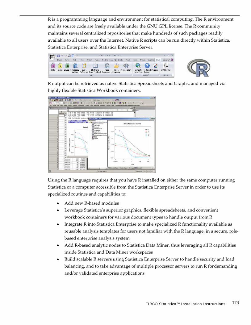
173 TIBCO Statistica™ Installation Instructions
R is a programming language and environment for statistical computing. The R environment and its source code are freely available under the GNU GPL license. The R community maintains several centralized repositories that make hundreds of such packages readily available to all users over the Internet. Native R scripts can be run directly within Statistica, Statistica Enterprise, and Statistica Enterprise Server.
R output can be retrieved as native Statistica Spreadsheets and Graphs, and managed via highly flexible Statistica Workbook containers.
Using the R language requires that you have R installed on either the same computer running Statistica or a computer accessible from the Statistica Enterprise Server in order to use its specialized routines and capabilities to:
• Add new R-based modules • Leverage Statistica’s superior graphics, flexible spreadsheets, and convenient
workbook containers for various document types to handle output from R • Integrate R into Statistica Enterprise to make specialized R functionality available as
reusable analysis templates for users not familiar with the R language, in a secure, role- based enterprise analysis system
• Add R-based analytic nodes to Statistica Data Miner, thus leveraging all R capabilities inside Statistica and Data Miner workspaces
• Build scalable R servers using Statistica Enterprise Server to handle security and load balancing, and to take advantage of multiple processor servers to run R for demanding and/or validated enterprise applications
174 TIBCO Statistica™ Installation Instructions
Recording Statistica Visual Basic (svb) Macros (Programs)
Analysis Macros, Master (Log) Macros, and Keyboard Macros Statistica provides a comprehensive selection of facilities for recording macros, such as Statistica Visual Basic (SVB) programs, to automate repetitive work or to be used as a means to automatically generate programs for further editing and modification. The macro programs recorded by these facilities can be saved to be run “as is,” or they can be used as the “building blocks” for more complex and highly customized Visual Basic application programs. Analysis Macros and Master Macros follow the identical syntax and can later be modified, but because of the different ways in which each of them is created, they offer distinctive advantages and disadvantages for specific applications.
Analysis macros. Simple Analysis Macros automatically record the settings, selections, and chosen options for a specific analysis. Note that the term “analysis” in Statistica denotes one task selected either from the Statistics, Data Mining, or Graphs tabs and can be very small and simple (for example, one scatterplot requested from the Graphs tab), or very elaborate (for example, a complex structural equation modeling analysis selected by choosing that option from the Statistics tab, and involving hundreds of output documents).
After selecting any of the statistical options from the Statistics or Data Mining tabs or graphics options from the Graphs tab, all actions such as variable selections, option settings, etc., are recorded “behind the scenes”; at any time you can transfer this recording (such as the Visual Basic code for that macro) to the Visual Basic Editor window. The Create Macro command is available from every analysis dialog via the drop-down menu displayed by clicking the Options button or the shortcut menu accessed by right-clicking the analysis button when the analysis is minimized.
Master macros (logs). You can record a Master Macro or Master Log of an entire session, which can consist of one or many analyses. This recording will “connect” analyses performed with various analysis options from the Statistics, Data Mining, and/or Graphs tabs. However, unlike simple Analysis Macros, you can turn the recording of Master Macros on and off.
The Master Macro recording will begin when you turn on the recording [select the Tools tab, click Macro, and select Start Recording Log of Analyses (Master Macro)], and it will end when you stop the recording (click Macro, and select Stop Recording). In between these actions, all file selections and data management operations are recorded, as are the analyses and selections for the analyses, in the sequence in which they were chosen.
Keyboard macros. This type of macro recording stores the sequences of keyboard input. When you select the Tools tab, click Macro, and select Start Recording Keyboard Macro, Statistica will record the actual keystrokes entered via the keyboard.
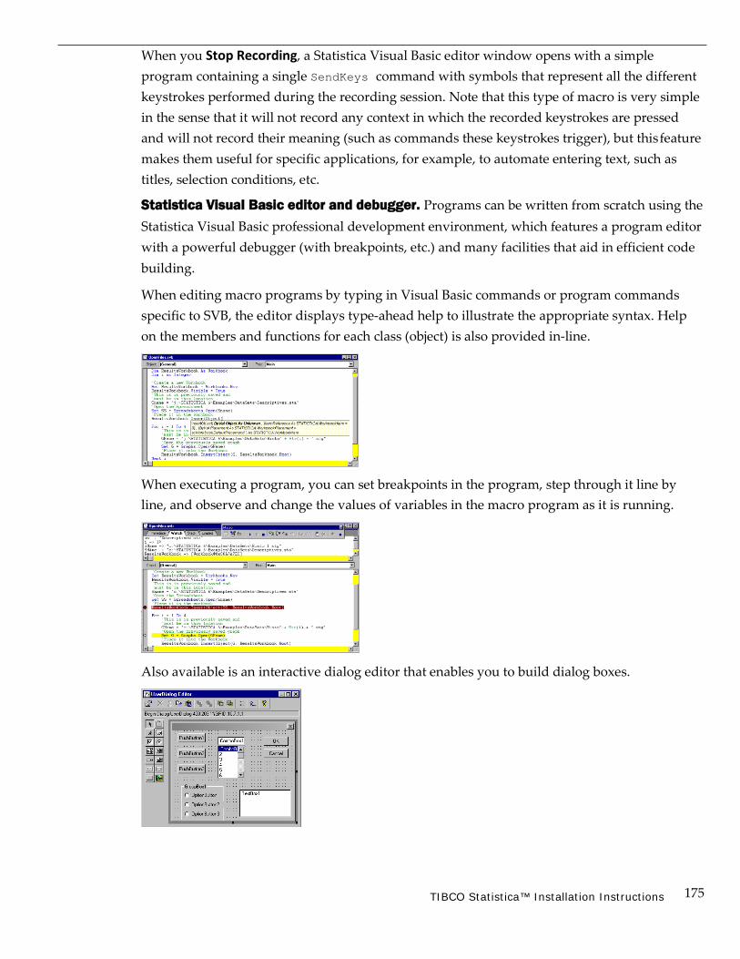
175 TIBCO Statistica™ Installation Instructions
When you Stop Recording, a Statistica Visual Basic editor window opens with a simple program containing a single SendKeys command with symbols that represent all the different keystrokes performed during the recording session. Note that this type of macro is very simple in the sense that it will not record any context in which the recorded keystrokes are pressed and will not record their meaning (such as commands these keystrokes trigger), but this feature makes them useful for specific applications, for example, to automate entering text, such as titles, selection conditions, etc.
Statistica Visual Basic editor and debugger. Programs can be written from scratch using the Statistica Visual Basic professional development environment, which features a program editor with a powerful debugger (with breakpoints, etc.) and many facilities that aid in efficient code building.
When editing macro programs by typing in Visual Basic commands or program commands specific to SVB, the editor displays type-ahead help to illustrate the appropriate syntax. Help on the members and functions for each class (object) is also provided in-line.
When executing a program, you can set breakpoints in the program, step through it line by line, and observe and change the values of variables in the macro program as it is running.
Also available is an interactive dialog editor that enables you to build dialog boxes.

176 TIBCO Statistica™ Installation Instructions
To summarize, Statistica Visual Basic is not only a powerful programming language, but it represents a very powerful, professional programming environment for developing simple macros as well as complex custom applications.
Visual Basic from other applications. SVB programs can also be developed by enhancing Visual Basic programs created in other applications (for example, Excel) by calling Statistica functions and procedures.
Executing Statistica Visual Basic Programs Statistica Visual Basic programs can be executed from within Statistica, but because of the industry standard compatibility of SVB, you can also execute its programs from any other compatible environment (for example, Excel, Word, or a stand-alone Visual Basic language). In practice, you would typically call Statistica functions from Visual Basic in another application.
Note, however, that when you run an SVB program or attempt to call Statistica functions from any other application, all calls to the Statistica specific functions (as opposed to the generic functions of MS Visual Basic) will be executed only if the respective Statistica libraries are present on the computer where the execution takes place. That is, you must be a licensed user of the respective Statistica libraries of procedures. Note that this large library of Statistica functions (more than 14,000 procedures) is transparently accessible not only to Visual Basic, but also to calls from any other compatible programming language or environment, such as C/C++, C#, or Delphi.
Performance of Statistica Visual Basic programs. While the obvious advantages of Visual Basic (compared to other languages) are its ease of use and familiarity to a very large number of computer users, the possible drawback of Visual Basic programs is that they do not perform as fast as applications developed in lower-level programming languages (such as C).
However, that potential problem does not apply to SVB applications, especially those that rely mostly on executing calls to Statistica’s analytic, graphics, and data management procedures. These procedures fully employ Statistica technology and perform at a speed comparable to running the respective procedures in Statistica directly.
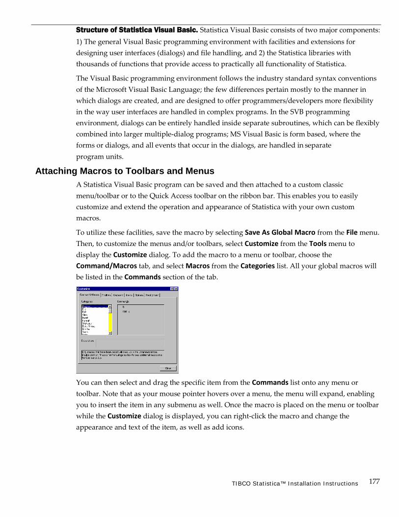
177 TIBCO Statistica™ Installation Instructions
Structure of Statistica Visual Basic. Statistica Visual Basic consists of two major components: 1) The general Visual Basic programming environment with facilities and extensions for designing user interfaces (dialogs) and file handling, and 2) the Statistica libraries with thousands of functions that provide access to practically all functionality of Statistica.
The Visual Basic programming environment follows the industry standard syntax conventions of the Microsoft Visual Basic Language; the few differences pertain mostly to the manner in which dialogs are created, and are designed to offer programmers/developers more flexibility in the way user interfaces are handled in complex programs. In the SVB programming environment, dialogs can be entirely handled inside separate subroutines, which can be flexibly combined into larger multiple-dialog programs; MS Visual Basic is form based, where the forms or dialogs, and all events that occur in the dialogs, are handled in separate program units.
Attaching Macros to Toolbars and Menus A Statistica Visual Basic program can be saved and then attached to a custom classic menu/toolbar or to the Quick Access toolbar on the ribbon bar. This enables you to easily customize and extend the operation and appearance of Statistica with your own custom macros.
To utilize these facilities, save the macro by selecting Save As Global Macro from the File menu. Then, to customize the menus and/or toolbars, select Customize from the Tools menu to display the Customize dialog. To add the macro to a menu or toolbar, choose the Command/Macros tab, and select Macros from the Categories list. All your global macros will be listed in the Commands section of the tab.
You can then select and drag the specific item from the Commands list onto any menu or toolbar. Note that as your mouse pointer hovers over a menu, the menu will expand, enabling you to insert the item in any submenu as well. Once the macro is placed on the menu or toolbar while the Customize dialog is displayed, you can right-click the macro and change the appearance and text of the item, as well as add icons.

178 TIBCO Statistica™ Installation Instructions
Running Macros from a command line. With Statistica, you can execute SVB programs from the command line by using the /RunMacro= command line parameter. The syntax is:
statist.exe /RunMacro=macroname
where “macroname” is the file name of the macro. If a full path is not specified, Statistica will attempt to run the macro from the application’s currently selected directory (which is Windows default behavior).
If the macro does not make the application or any document visible (through the Application.Visible = True, or similar document properties), the STATISITCA instance will automatically shut down when complete. If the application is made visible, the application will remain visible after the macro completes, and you will need to shut down the program.
Example: Recording an Analysis This example illustrates how to record an analysis into a script that can be executed to re-run the analysis. Then the script will be edited and combined with another script to create a customized script that can run analyses on demand. Additionally, this example shows how you can use attached scripts to auto-update and re-run analyses from results workbooks.
Start by opening the example Adstudy data set. Select the Home tab, click the Open arrow, and select Open Examples to display the Open a Statistica Data File dialog. Double-click on the Datasets file, and then open the Statistica data set Adstudy.sta.
Then, select the Statistics tab. In the Base group, click Basic Statistics to display the Basic Statistics and Tables Startup Panel. Select Descriptive statistics.
Click the OK button to display the Descriptive Statistics dialog.
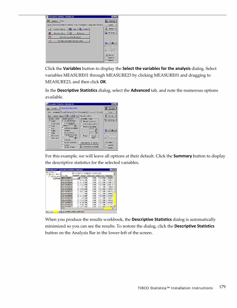
179 TIBCO Statistica™ Installation Instructions
Click the Variables button to display the Select the variables for the analysis dialog. Select variables MEASURE01 through MEASURE23 by clicking MEASURE01 and dragging to MEASURE23, and then click OK.
In the Descriptive Statistics dialog, select the Advanced tab, and note the numerous options available.
For this example, we will leave all options at their default. Click the Summary button to display the descriptive statistics for the selected variables.
When you produce the results workbook, the Descriptive Statistics dialog is automatically minimized so you can see the results. To restore the dialog, click the Descriptive Statistics button on the Analysis Bar in the lower-left of the screen.
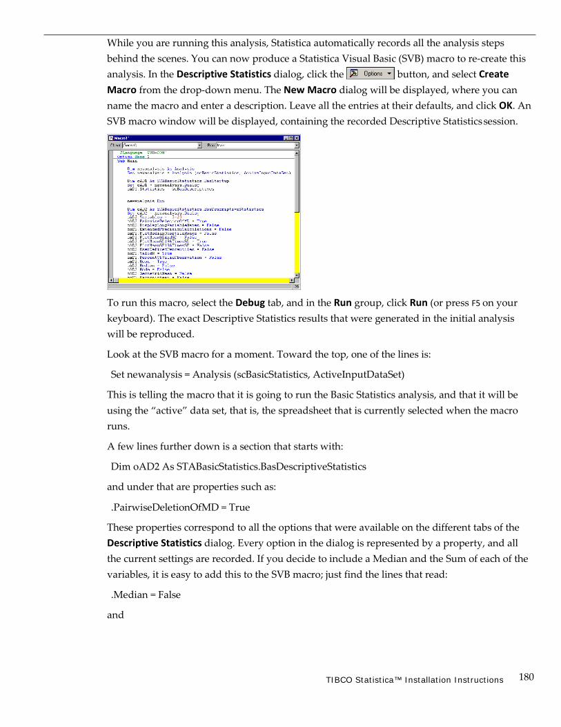
180 TIBCO Statistica™ Installation Instructions
While you are running this analysis, Statistica automatically records all the analysis steps behind the scenes. You can now produce a Statistica Visual Basic (SVB) macro to re-create this analysis. In the Descriptive Statistics dialog, click the button, and select Create Macro from the drop-down menu. The New Macro dialog will be displayed, where you can name the macro and enter a description. Leave all the entries at their defaults, and click OK. An SVB macro window will be displayed, containing the recorded Descriptive Statistics session.
To run this macro, select the Debug tab, and in the Run group, click Run (or press F5 on your keyboard). The exact Descriptive Statistics results that were generated in the initial analysis will be reproduced.
Look at the SVB macro for a moment. Toward the top, one of the lines is:
Set newanalysis = Analysis (scBasicStatistics, ActiveInputDataSet)
This is telling the macro that it is going to run the Basic Statistics analysis, and that it will be using the “active” data set, that is, the spreadsheet that is currently selected when the macro runs.
A few lines further down is a section that starts with:
Dim oAD2 As STABasicStatistics.BasDescriptiveStatistics
and under that are properties such as:
.PairwiseDeletionOfMD = True
These properties correspond to all the options that were available on the different tabs of the Descriptive Statistics dialog. Every option in the dialog is represented by a property, and all the current settings are recorded. If you decide to include a Median and the Sum of each of the variables, it is easy to add this to the SVB macro; just find the lines that read:
.Median = False
and

181 TIBCO Statistica™ Installation Instructions
.Sum = False
and change these to:
.Median = True
and
.Sum = True
Now, run the macro again by pressing F5. A new results spreadsheet will be added to the workbook, this time with new columns of Median and Sum:
Let’s keep the macro window open and start a new analysis on the same sample data set. Select the Adstudy spreadsheet to bring it to the front. Select the Graphs tab, and in the More group, click 2D. Select Normal Probability Plots to display the Normal Probability Plots dialog.
Click the Variables button, and in the Select Variables for Probability Plot dialog, select variables MEASURE01 through MEASURE03. Click OK to close this dialog, and click OK in the Normal Probability Plots dialog. Three Probability Plot graphs will be placed in the results workbook, one for each of the three variables that were selected.

182 TIBCO Statistica™ Installation Instructions
The steps of the Probability Plot analysis were recorded just as they were for the Descriptive Statistics analysis. To create a new macro with these steps, bring the Normal Probability Plot dialog to the front by clicking that button on the Analysis Bar in the lower-left of the screen, click the button, and select Create Macro from the drop-down menu. In the New Macro dialog, click OK, and a new SVB Macro window is opened with the recorded Probability Plot script.
As with the Descriptive Statistics analysis, all the options selected in the Probability Plot dialog are specified as properties within the macro. For instance, to change this from a Normal Probability Plot to a Half Normal Probability Plot, locate the following line:
.GraphType = scProbNormal
and change it to:
.GraphType = scProbHalfNormal
Also, let’s expand the variables to include variable MEASURE04. To do this, find the following line:
.Variables = "3-5"
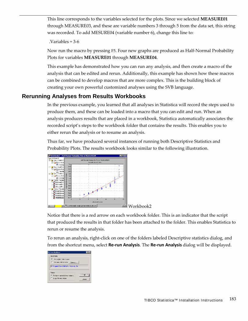
183 TIBCO Statistica™ Installation Instructions
This line corresponds to the variables selected for the plots. Since we selected MEASURE01 through MEASURE03, and these are variable numbers 3 through 5 from the data set, this string was recorded. To add MESURE04 (variable number 6), change this line to:
.Variables = 3-6
Now run the macro by pressing F5. Four new graphs are produced as Half-Normal Probability Plots for variables MEASURE01 through MEASURE04.
This example has demonstrated how you can run any analysis, and then create a macro of the analysis that can be edited and rerun. Additionally, this example has shown how these macros can be combined to develop macros that are more complex. This is the building block of creating your own powerful customized analyses using the SVB language.
Rerunning Analyses from Results Workbooks In the previous example, you learned that all analyses in Statistica will record the steps used to produce them, and these can be loaded into a macro that you can edit and run. When an analysis produces results that are placed in a workbook, Statistica automatically associates the recorded script’s steps to the workbook folder that contains the results. This enables you to either rerun the analysis or to resume an analysis.
Thus far, we have produced several instances of running both Descriptive Statistics and Probability Plots. The results workbook looks similar to the following illustration.
Workbook2
Notice that there is a red arrow on each workbook folder. This is an indicator that the script that produced the results in that folder has been attached to the folder. This enables Statistica to rerun or resume the analysis.
To rerun an analysis, right-click on one of the folders labeled Descriptive statistics dialog, and from the shortcut menu, select Re-run Analysis. The Re-run Analysis dialog will be displayed.

184 TIBCO Statistica™ Installation Instructions
Here you can choose to Use original data source or Use new data source. The latter option gives you the powerful ability to create templates that can then be applied to new data sources. In addition to specifying the data source, you can choose to Replace current folder contents or Output to new folder. In this example, leave the defaults, and click OK. You will see that the contents of the folder are briefly deleted and then added again as the analysis is rerun.
One purpose for this feature is the ability to update/rerun results from complex analyses if new data is entered into the spreadsheet. For instance, if the data in the open data file Adstudy.sta has been changed and the analysis is rerun, the new results will be calculated with the new data.
The resume analysis functionality enables you to bring an analysis back to the point before the results were generated, allowing you to select different options or continue an analysis in progress.
Right-click the same Descriptive statistics dialog folder, and from the shortcut menu, select Resume Analysis. The Resume Analysis dialog will be displayed. This dialog also contains options to specify the input data source (original or new). The Output options for the new results are to Output to current folder (as if this is just an extension of the previous analysis) or Output to new folder (as if this is a brand new analysis).
Leave the defaults as they are, and click OK. The Descriptive Statistics dialog will be displayed, with all the options set to what was used when the selected output was created. Since the default was to Output to current folder, clicking the Summary button will generate new output to the same folder.
ACTIVEX Objects and Documents (A Technical Note) The term ActiveX is used in different contexts, and its definitions stress different aspects of that concept. Its use within Statistica, however, can be grouped into two general categories: ActiveX objects and ActiveX documents.
ActiveX objects. An ActiveX object is what was once referred to as an OLE (Object Linking and Embedding) object. At its heart is the Microsoft COM (Component Object Model) technology that makes it possible for objects to be accessed in a uniform manner.

185 TIBCO Statistica™ Installation Instructions
Through the use of standard protocols, objects created in one application can be stored and edited in a different application. To support this functionality, the containing object needs to be an ActiveX object client, and the application that initially created the object needs to be an ActiveX object server. Statistica is both. As an ActiveX object client, Statistica allows you to embed and link objects from other applications in spreadsheets, graphs, and reports. As an ActiveX object server, it allows you to embed and link spreadsheets and graphs into other applications.
ActiveX documents. ActiveX documents take the ActiveX controls one step further, in that they allow entire documents to be embedded into other applications. An ActiveX document container allows other application documents to be used within it, and an ActiveX document server allows its documents to be used within any ActiveX document container.
Again, Statistica does both. Statistica Workbooks are ActiveX document containers, and allow documents from other ActiveX servers to be displayed within the workbook. Examples of this are Word and Excel; these documents can be used directly from within a Statistica Workbook. Similarly, Statistica Spreadsheets, Graphs, and Reports are ActiveX document servers, and they also can be placed within any ActiveX document container such as Microsoft Internet Explorer.
Office integration and ActiveX documents. The ActiveX document technology has special application with Word and Excel documents. Statistica can open these particular documents natively in their own windows within the Statistica workspace. This “Office integration”
enables you to use Excel documents as data sources and Word documents as reports for analyses. When the documents are open in the Statistica window, the appropriate menus and toolbars for Excel/Word are available for use.
186 TIBCO Statistica™ Installation Instructions
Chapter Nine Statistica Query

187 TIBCO Statistica™ Installation Instructions
This chapter includes a brief overview of Statistica Query, a flexible tool for accessing data from external databases. It also includes information on retrieving data from OLAP Cube providers such as MS OLE DB Provider for Analysis Services or SAP Business Warehouse MDX.
Overview Statistica Query is used to access data easily from a wide variety of databases (including many large system databases such as Oracle, MS SQL Server, Sybase, etc.) using Microsoft’s OLE DB conventions. OLE DB is a powerful database technology that provides universal data integration over an enterprise’s network, from mainframe to desktop, regardless of the data type. OLE DB offers a more generalized and more efficient strategy for data access than the older ODBC conventions because it allows access to more types of data and is based on the Component Object Model (COM).
Statistica Query supports multiple database tables; specific records (rows of tables) can be selected by entering SQL statements, which Statistica Query automatically builds for you as you select the components of the query via a simple graphical interface and/or intuitive menu options and dialogs.
Therefore, an extensive knowledge of SQL is not necessary in order for you to create advanced and powerful queries of data in a quick and straightforward manner. Multiple queries based on one or many different databases can also be created to return data to an individual spreadsheet, and you can maintain connections to multiple external databases simultaneously.
Statistica Query: Quick Step-by-Step Instructions The steps necessary to retrieve external data via Statistica Query are outlined below:
1. Select the Home tab. In the File group, click the Open arrow. Select Open External Data - Create Query to display the Database Connection dialog. (You can also select the Data tab. In the Manage group, click External Data and select Create Query to display the Database Connection dialog.) In this dialog, select a predefined database connection (the provider, data source location, and advanced settings of the server or directory on which the data resides).
Note that if you have not already created the database connection, you can do so by clicking the New button in the Database Connection dialog. The Data Link Properties dialog will be displayed, which will guide you through a step-by-step wizard to create a database connection. For specific documentation when you are using the Data Link Properties dialog, press the F1 key on your keyboard to display the Microsoft Data Link Help®.

188 TIBCO Statistica™ Installation Instructions
2. After you have selected a database connection and clicked the OK button in the Data Link Properties dialog, you will have access to Statistica Query in which you can create a SQL statement by specifying the desired tables, fields, joins, criteria, etc. (via the Table, Join, and Criteria menus) to be included in your query.
3. Once you have specified a query, select Return Data to Statistica from the File menu. The Returning External Data to Spreadsheet dialog will be displayed, in which you can specify the name of the query, where you want Statistica Query to put the data that the query returns, and additional options.
In-Place Processing of Data on Remote Servers (the IDP Technology Option)
The query facilities (described in the previous sections), when offered as part of the enterprise versions of Statistica are additionally enhanced by options to process data from remote servers in-place, that is, without having to import them and create a local data file. This In-Place Database Processing (IDP) technology is particularly useful for processing extremely large data files where it can produce significant performance gains and enable Statistica users to process data files that exceed the storage capacity of the local device or even the Statistica Enterprise Server.
Technical note. The IDP technology is based on distributed processing architecture, where the queries are performed on the server side (using the server CPU resources) and the respective records sent to the Statistica computer where they are simultaneously (asynchronously) processed as they become available.
189 TIBCO Statistica™ Installation Instructions
OLAP CUBES OLAP (On-Line Analytic Processing) is a generic term for a system that provides efficient access to summary data about very large databases. Unlike ordinary relational databases, which organize data as a set of well-defined, two-dimensional tables, an OLAP data warehouse represents data at many levels of detail in multi-dimensional data sets known as cubes.
When a Statistica user wants to perform an analysis against data from an OLAP Cube, the data must be reduced to a two-dimensional form – cases and variables – that can be represented in a Statistica spreadsheet. The Statistica Query tool provides a graphical, drag-and-drop interface for specifying the dimensions and levels of detail that will be extracted from the cube to feed into the query. The “MDX” (Multi-Dimensional eXpressions) mode is triggered automatically when an OLAP data source is selected.
Customers who require OLAP integration will usually have sophisticated database support technicians through their in-house information technology department who can help design these queries. Because the configuration of the dimensions in an OLAP cube is determined by the customer’s database administrators, Statistica can provide only limited assistance in this area.
Large Database Files Statistica products are designed for large-scale analytics; consequently, they integrate well with database systems designed for managing very large amounts of data, such as Teradata and others. For example, Statistica can both extract data for analysis from Teradata, and it can also score results directly inside Teradata through deployment code created by Statistica Data Miner and applied to the Teradata as a user-defined function, which significantly accelerates processing of large amounts of data.

190 TIBCO Statistica™ Installation Instructions
Chapter Ten Programming Statistica from .NET

191 TIBCO Statistica™ Installation Instructions
Virtually every aspect of Statistica is exposed as a set of COM interfaces that are registered on a machine when Statistica is installed. Since .NET-based languages cannot communicate with COM directly, a wrapper class called the COM Interop can be utilized to integrate the Statistica libraries into your .NET project. The COM Interop layer is created automatically by the
Visual Studio .NET IDE when you import a COM interface. The COM Interop layer handles all of the details regarding interacting with the COM libraries in .NET. With the COM Interop layer in place, the Statistica COM interfaces behave like any other .NET object.
Adding the Statistica Object Library into Your .NET Project The .NET Interop layer is created automatically by adding the desired Statistica COM interfaces into your .NET project. Statistica Object Library is the base Statistica COM library. To add the Statistica Object Library to a .NET project, first select the desired .NET project in Solution Explorer, and then select Add Reference from the shortcut menu (accessed by right- clicking on the .NET project).
The Add Reference dialog will be displayed. Select the COM tab. From the Component Name list, select Statistica Object Library, and click OK.
At this point, the necessary COM Interop library is created automatically. Under the project References node, you will now see the entry Statistica.
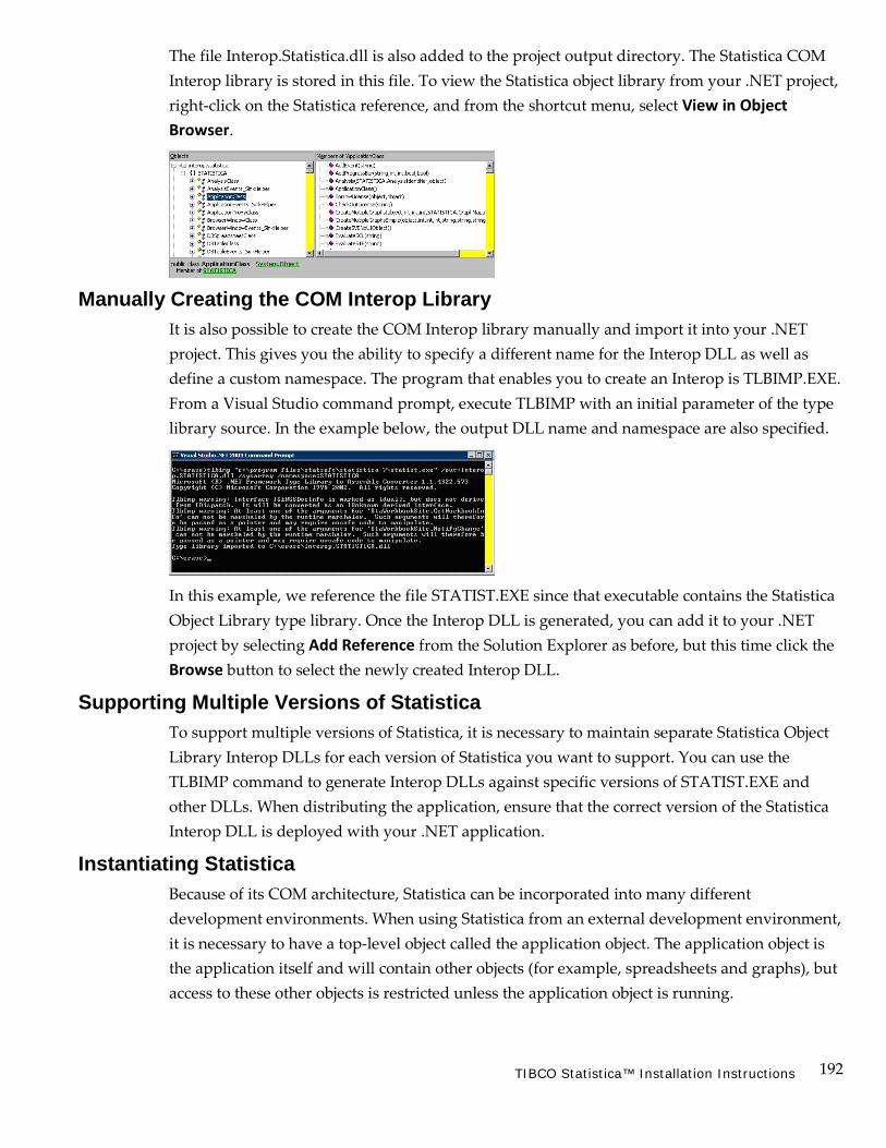
192 TIBCO Statistica™ Installation Instructions
The file Interop.Statistica.dll is also added to the project output directory. The Statistica COM Interop library is stored in this file. To view the Statistica object library from your .NET project, right-click on the Statistica reference, and from the shortcut menu, select View in Object Browser.
Manually Creating the COM Interop Library It is also possible to create the COM Interop library manually and import it into your .NET project. This gives you the ability to specify a different name for the Interop DLL as well as define a custom namespace. The program that enables you to create an Interop is TLBIMP.EXE. From a Visual Studio command prompt, execute TLBIMP with an initial parameter of the type library source. In the example below, the output DLL name and namespace are also specified.
In this example, we reference the file STATIST.EXE since that executable contains the Statistica Object Library type library. Once the Interop DLL is generated, you can add it to your .NET project by selecting Add Reference from the Solution Explorer as before, but this time click the Browse button to select the newly created Interop DLL.
Supporting Multiple Versions of Statistica To support multiple versions of Statistica, it is necessary to maintain separate Statistica Object Library Interop DLLs for each version of Statistica you want to support. You can use the TLBIMP command to generate Interop DLLs against specific versions of STATIST.EXE and other DLLs. When distributing the application, ensure that the correct version of the Statistica Interop DLL is deployed with your .NET application.
Instantiating Statistica Because of its COM architecture, Statistica can be incorporated into many different development environments. When using Statistica from an external development environment, it is necessary to have a top-level object called the application object. The application object is the application itself and will contain other objects (for example, spreadsheets and graphs), but access to these other objects is restricted unless the application object is running.
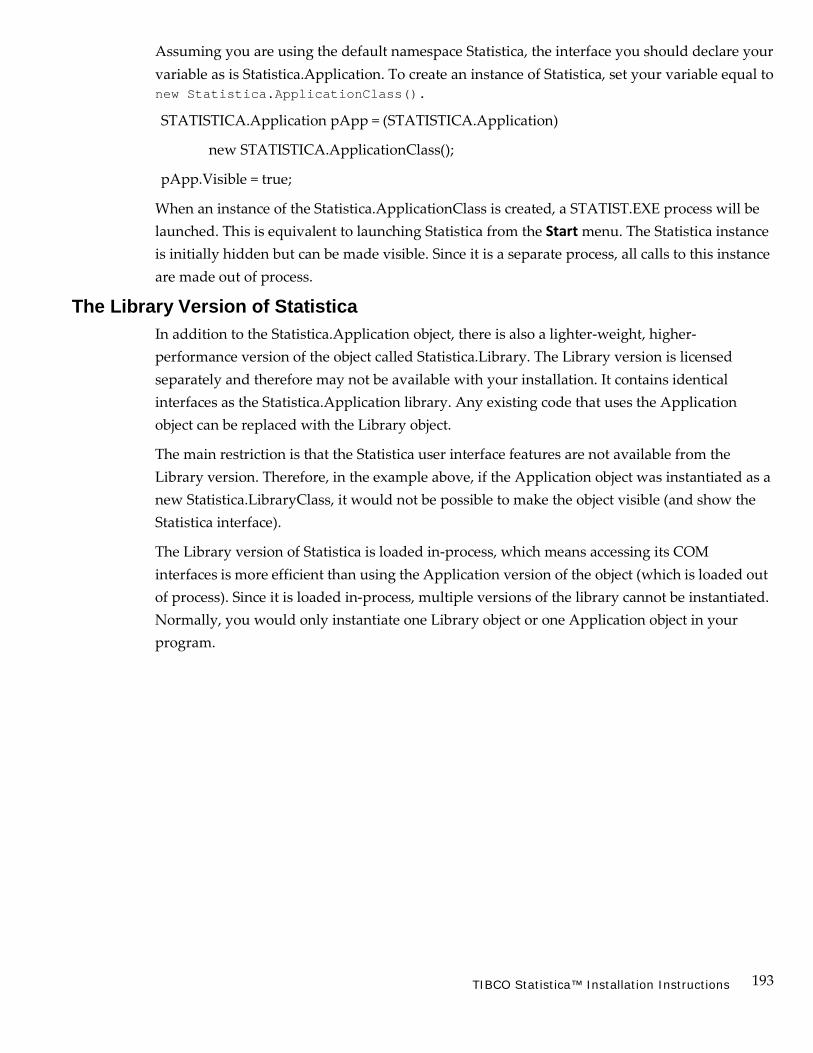
193 TIBCO Statistica™ Installation Instructions
Assuming you are using the default namespace Statistica, the interface you should declare your variable as is Statistica.Application. To create an instance of Statistica, set your variable equal to new Statistica.ApplicationClass().
STATISTICA.Application pApp = (STATISTICA.Application)
new STATISTICA.ApplicationClass();
pApp.Visible = true;
When an instance of the Statistica.ApplicationClass is created, a STATIST.EXE process will be launched. This is equivalent to launching Statistica from the Start menu. The Statistica instance is initially hidden but can be made visible. Since it is a separate process, all calls to this instance are made out of process.
The Library Version of Statistica In addition to the Statistica.Application object, there is also a lighter-weight, higher- performance version of the object called Statistica.Library. The Library version is licensed separately and therefore may not be available with your installation. It contains identical interfaces as the Statistica.Application library. Any existing code that uses the Application object can be replaced with the Library object.
The main restriction is that the Statistica user interface features are not available from the Library version. Therefore, in the example above, if the Application object was instantiated as a new Statistica.LibraryClass, it would not be possible to make the object visible (and show the Statistica interface).
The Library version of Statistica is loaded in-process, which means accessing its COM interfaces is more efficient than using the Application version of the object (which is loaded out of process). Since it is loaded in-process, multiple versions of the library cannot be instantiated. Normally, you would only instantiate one Library object or one Application object in your program.
194 TIBCO Statistica™ Installation Instructions
Appendix A Statistica Enterprise Server
195 TIBCO Statistica™ Installation Instructions
Statistica Enterprise Server is a highly scalable, enterprise-level, fully Web-enabled data analysis and database gateway application system that is built on distributed processing technology and fully supports multi-tier Client-Server architecture configurations. Statistica Enterprise Server exposes the analytic, query, reporting, and graphics functionality of Statistica through easy-to-use, interactive, standard Web interfaces. Alternatively, it enables users of the desktop version (thick client) to offload computationally intensive analytics and database operations to the Server. It is offered as a complete, ready-to-install application with an interactive, Internet browser-based (point-and-click) user interface (thin client) that makes it possible for users to interactively create data sets, run analyses, and review output.
However, Statistica Enterprise Server is built using open architecture and includes .NET- compatible development kit tools (based entirely on industry standard syntax conventions such as VB Script, C++/C#, HTML, Java, and XML) that enables IT department personnel to customize all main components of the system or expand it by building on its foundations, for example, by adding new components and/or company-specific analytic or database facilities.
As mentioned, Statistica Enterprise Server is provided with an Internet browser-based user interface (in the form of simple-to-navigate and easy-to-use dialogs) enabling you to specify analyses and review results. However, tools are provided to customize these dialogs and easily set up new user interfaces or to add new functions. For example, a simple dialog with only three buttons can be created in the browser, and clicking each button will run a series of analyses and generate a detailed report. Statistica Enterprise Server applications add a new dimension and an endless array of possibilities to the entire line of Statistica Data Analysis, Data Mining, and Quality Control/Six Sigma software.
The system is compatible with all major Web server software platforms (for example, UNIX Apache, and Microsoft IIS), works in both Microsoft .NET and Sun/Java environments, and does not require any changes to the existing firewall and Internet/Intranet security systems.
A Broad Choice of Analytic Facilities and Configurations
The Statistica Enterprise Server system is offered as a complete solution that includes the analytic functionality of any Statistica product or any combination of products, from Statistica Base to Data Miner applications.
The minimum installation of Statistica Enterprise Server software includes the analytic functionality of Statistica Base and a license for 5 concurrent users (minimum).
Customers can either order a specific version of Statistica Enterprise Server including the analytic functionality that they require (for example, Statistica Base for 10 users), or they can add the Enterprise Server functionality (as described in this section) to some or all of the seats of the currently licensed Statistica product (for example, add the Enterprise Server functionality to 20 out of 50 existing licenses of Statistica Enterprise).
196 TIBCO Statistica™ Installation Instructions
Functionality and Applications: The Advantages of Statistica Enterprise Server
A powerful, enterprise-wide collaborative-intelligence system. Another important way to take advantage of the Statistica Enterprise Server functionality is to use it as the core and natural extension of any of the Statistica enterprise systems (for example, Statistica Data Miner applications).
Specifically, Statistica Enterprise Server can act as the core of an enterprise-wide network system that enables the participants to work collaboratively and quickly share results (reports), as well as scripts of analyses or queries. User or group permissions (see the Technical Note on page 203) can be used by the administrators to manage access of specific groups of users to specific data or reports. The accessibility of its tools makes Statistica Enterprise Server a perfect system to facilitate collaborative projects of employees who are telecommuting or traveling.
Advantages of distributed processing, and multi-tier Client-Server architecture. Users will benefit not only from the collaborative work tools but also the options to offload the computationally intensive or time-consuming tasks to the server computers. Specifically, because the most powerful multiprocessor CPUs (and/or clusters of computers) are usually used as servers, users can offload computationally intensive tasks, and, for example, run in the background queries that will scan terabytes of data on remote servers and perform time-consuming, long sequences of analyses or reports, while keeping the end users’ computers completely free to do other tasks. Because of its distributed processing architecture, Statistica Enterprise Server scales in a highly efficient manner to take advantage of multi-processor CPUs and/or multiple computers and, therefore, users can take full advantage of multi-tier Client-Server architecture, where:
• Tier 1 is the user interface on the client computer (a plain browser or Statistica thick client, see Statistica Client, page 197),
• Tier 2 is the Statistica Enterprise Server software and the implementation of the “business intelligence” that it may contain (specific queries, scripts of custom/proprietary analyses, etc.), and
• Tier 3 is Statistica databases (for example, Statistica Data Warehouse) or other corporate repositories of data.
In the desktop version of Statistica, all computations are performed on the local computer, and resources of other computers are used only in the case when the In-Place Database Processing (IDP), see page 188, interface to external databases is established. IDP is a technology that reads data asynchronously directly from remote database servers (using distributed processing if supported by the server), and bypasses the need to “import” data and create a local copy of the data set. Records of data are retrieved and sent to the Statistica computer asynchronously by the CPU of the database server, while Statistica simultaneously processes them using the CPU of the local computer.
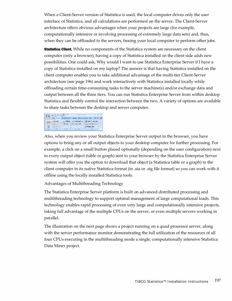
197 TIBCO Statistica™ Installation Instructions
When a Client-Server version of Statistica is used, the local computer drives only the user interface of Statistica, and all calculations are performed on the server. The Client-Server architecture offers obvious advantages when your projects are large (for example, computationally intensive or involving processing of extremely large data sets) and, thus, when they can be offloaded to the servers, freeing your local computer to perform other jobs.
Statistica Client. While no components of the Statistica system are necessary on the client computer (only a browser), having a copy of Statistica installed on the client side adds new possibilities. One could ask, Why would I want to use Statistica Enterprise Server if I have a copy of Statistica installed on my laptop? The answer is that having Statistica installed on the client computer enables you to take additional advantage of the multi-tier Client-Server architecture (see page 196) and work interactively with Statistica installed locally while offloading certain time-consuming tasks to the server machine(s) and/or exchange data and output between all the three tiers. You can run Statistica Enterprise Server from within desktop Statistica and flexibly control the interaction between the two. A variety of options are available to share tasks between the desktop and server computer.
Also, when you review your Statistica Enterprise Server output in the browser, you have options to bring any or all output objects to your desktop computer for further processing. For example, a click on a small button placed optionally (depending on the user configuration) next to every output object (table or graph) sent to your browser by the Statistica Enterprise Server system will offer you the option to download that object (a Statistica table or a graph) to the client computer in its native Statistica format (in .sta or .stg file format) so you can work with it offline using the locally installed Statistica tools.
Advantages of Multithreading Technology
The Statistica Enterprise Server platform is built on advanced distributed processing and multithreading technology to support optimal management of large computational loads. This technology enables rapid processing of even very large and computationally intensive projects, taking full advantage of the multiple CPUs on the server, or even multiple servers working in parallel.
The illustration on the next page shows a project running on a quad processor server, along with the server performance monitor demonstrating the full utilization of the resources of all four CPUs executing in the multithreading mode a single, computationally intensive Statistica Data Miner project.
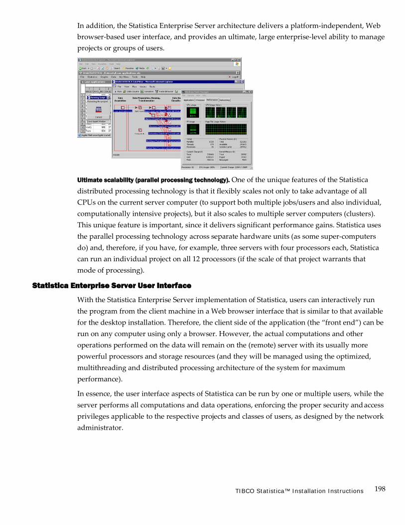
198 TIBCO Statistica™ Installation Instructions
In addition, the Statistica Enterprise Server architecture delivers a platform-independent, Web browser-based user interface, and provides an ultimate, large enterprise-level ability to manage projects or groups of users.
Ultimate scalability (parallel processing technology). One of the unique features of the Statistica distributed processing technology is that it flexibly scales not only to take advantage of all CPUs on the current server computer (to support both multiple jobs/users and also individual, computationally intensive projects), but it also scales to multiple server computers (clusters). This unique feature is important, since it delivers significant performance gains. Statistica uses the parallel processing technology across separate hardware units (as some super-computers do) and, therefore, if you have, for example, three servers with four processors each, Statistica can run an individual project on all 12 processors (if the scale of that project warrants that mode of processing).
Statistica Enterprise Server User Interface
With the Statistica Enterprise Server implementation of Statistica, users can interactively run the program from the client machine in a Web browser interface that is similar to that available for the desktop installation. Therefore, the client side of the application (the “front end”) can be run on any computer using only a browser. However, the actual computations and other operations performed on the data will remain on the (remote) server with its usually more powerful processors and storage resources (and they will be managed using the optimized, multithreading and distributed processing architecture of the system for maximum performance).
In essence, the user interface aspects of Statistica can be run by one or multiple users, while the server performs all computations and data operations, enforcing the proper security and access privileges applicable to the respective projects and classes of users, as designed by the network administrator.

199 TIBCO Statistica™ Installation Instructions
Statistica Enterprise Server offers a straightforward user interface supporting a selection of interactive data analysis, data mining, quality control, database management, database query, and graph customization operations.
After logging on to the Statistica Enterprise Server system,
you can select a data source (a data set or a live database connection),
review and edit the data in the interactive Spreadsheet Editor,
select the analysis to be performed using the standard menu system (or a shortcut in the user- defined My Menu),

200 TIBCO Statistica™ Installation Instructions
select variables and specify optional analysis parameters,
and interactively review the output.
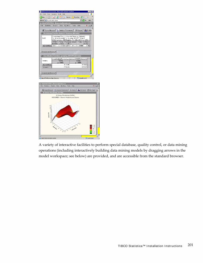
201 TIBCO Statistica™ Installation Instructions
A variety of interactive facilities to perform special database, quality control, or data mining operations (including interactively building data mining models by dragging arrows in the model workspace; see below) are provided, and are accessible from the standard browser.

202 TIBCO Statistica™ Installation Instructions
In addition to these built-in, straightforward user-interface facilities, Statistica Enterprise Server also includes a toolkit that enables users to customize the user interface and develop custom applications with specifically predefined functionality, packaged in a way that matches the requirements of their specific applications.
Compatibility with Industry Standards

203 TIBCO Statistica™ Installation Instructions
The unsurpassed compatibility with industry standards is another in the long list of unique advantages of Statistica Enterprise Server.
Statistica Enterprise Server can be deployed on any of the popular Web server platforms (for example, a UNIX-based Apache or IIS), and therefore, it will conform to the existing local security protocols (fire walls) as required by the corporate client.
Statistica Enterprise Server uses advanced proprietary technology developed at Statistica to ensure its high performance and scalability (for example, multiple, multiprocessor Statistica Enterprise Server computers working in a distributed processing environment). This technology is built on Statistica’s years of experience providing high performance, scalable enterprise systems to major corporations in the United States and around the world. However, Statistica Enterprise Server is still based on the industry standard communication protocols (for example, XML) to ensure 1) its platform independence, 2) smooth transition to future technologies, and 3) ease of customization by the client. Note that the ease of customization is additionally boosted by the fact that only the industry standard syntax conventions (such as VB script, C++, HTML, and XML) are used to customize, configure, and define all the specific analytic operations and all output in Statistica Enterprise Server.
Architecture of the System (A Technical Note)
Although the general design uses two computers in a typical configuration, the Web server (for example, a UNIX-based Apache system) and at least one Statistica Enterprise Server (optionally scalable to multiple Statistica Enterprise Servers),
in many cases, Statistica Enterprise Server could be installed on the same machine if desired (when IIS is used as the Web host):

204 TIBCO Statistica™ Installation Instructions
The design allows for a flexible, generic Web server implementation by using a standard scripting language on the Web server. The purpose of the Web server is to package requests from the user (received from a browser), send these to the Statistica Enterprise Server, and then process responses from the Statistica Enterprise Server for display to the users (on their browsers).
Communication between the Web server and the Statistica Enterprise Server is accomplished through technology based on the industry standard XML conventions. The system is fully customizable, and for customers who want to develop their own modifications or extensions of this (ready-to-deploy) system, it provides development tool kit facilities allowing modification of all aspects of both the scripts that are being executed by Statistica (on the Statistica Enterprise Server side) and the appearance of the user interface exposed to the end users on the (browser-based) thin client side. Only the most standard, commonly known tools (such as VB or XML/HTML) are used to customize or expand the system.
The actual Web page definitions and Statistica scripts to be executed are stored in a designated Repository Facility on the Statistica Enterprise Server, and they are managed in a queue-like fashion. The system also includes a highly optimized Distributed Processing Manager that handles the incoming processing load and distributes it optimally over multiple threads of Statistica and multiple Statistica Enterprise Server computers.
The Statistica Enterprise Server software system also includes the Statistica Visual Basic Web Extensions. These extensions to the SVB language enable the script writer to either let the system display the resulting graphs and spreadsheets on the automatically generated (output) Web pages, or customize the appearance of the generated output pages by adding HTML directives as appropriate.
Security and authentication is a key design feature in the Statistica Enterprise Server application system. At the beginning of the session, users “sign on” to the system with their user name and password. System administrators are able to control access to data sources and scripts based either on user or group permissions.
The highest level of the access privilege allows advanced users (or administrators) to execute virtually arbitrary scripts (for example, in order to perform system administration or maintenance operations). This level requires a designated (highest) access privilege because, due to the general nature and power of the Statistica Visual Basic language, it gives access (to the authorized users) to all resources on the network.
Note that this system can be integrated with the “traditional” (such as non-Web-based) Statistica concurrent network or a Statistica enterprise system authentication scheme.

205 TIBCO Statistica™ Installation Instructions
Competitive Advantages
The competitive advantages of Statistica Enterprise Server applications start with the complete list of unique features of Statistica itself. Further, unlike the competing products, we offer a complete application (a “solution”) with a Web-based user interface and not merely a “development kit” (although the development kit facilities are also available to extend or customize the system). Also, we do not require that a specific Web server software be installed first (which may or may not comply with the client’s security standards and other policies). Finally, our system is controlled by industry standard VB scripts, C++, HTML, and XML that can be easily modified by users or system administrators. In addition, our distributed processing and multithreading technology delivers performance and system responsiveness that is not matched by any competing products.
Knowledge Portal
A designated Knowledge Portal application is optionally available that enables users to effectively and securely distribute organized sets of output documents over the Web. It offers support for workgroups of users (each with different access privileges, and thus access to different parts of the database of output documents), intuitive tree-view organization of available materials, and options to broadcast documents updated on the Web server in real time.
Statistica Enterprise Server Demo Movie
How does Statistica Enterprise Server work? Visit Statistica’s Web site, http://statistica.io/, to view an informative presentation of the unique features of Statistica described here. The movie also includes a step-by-step example application.