tick size change in the wholesale foreign exchange marketrgencay/jarticles/ticksizefx.pdf · tick...
TRANSCRIPT
Tick Size Change in the Wholesale
Foreign Exchange Market
Soheil Mahmoodzadeh∗, Ramazan Gencay
October 1, 2014
Department of Economics, Simon Fraser University, BC, Canada.
Abstract
This paper studies the changes in the spread, market depth and market efficiency that are dueto the lower minimum tick size (which was changed from a pip to a decimal pip) in the ElectronicBroking Services (EBS) interbank foreign exchange (FX) market. Coupled with the lower tick size,the composition of the traders and their order placement strategies have given an opportunity tohigh frequency traders (HFTs) to implement the sub-penny jumping strategy to front-run manualtraders. Our analysis shows that the lower tick size enabled HFTs to be more aggressive in thesub-penny jumping strategy. We show by difference-in-difference (DID) regression that the spreadas a liquidity cost was reduced after the tick size change. Furthermore, the benefit of the reductionin the spread was mostly absorbed by the HFTs, whereas the manual traders faced wider spreads.More strikingly, the market depth was reduced significantly after the introduction of decimal pippricing. There was no distinctive change in the arbitrage opportunities as a sign of market efficiency.
JEL classification: F31; G14; G15.
Keywords: Foreign Exchange Market; Tick Size; Market Microstructure
∗Corresponding author: Soheil Mahmoodzadeh ([email protected]). We are thankful to Alain Chaboud, AlecSchmidt and the participants in the seminars at Simon Fraser University. Ramazan Gencay ([email protected]) grate-fully acknowledges financial support from the Natural Sciences and Engineering Research Council of Canada and theSocial Sciences and Humanities Research Council of Canada. The remaining errors are ours.
1. Introduction
We study changes in market quality that are due to the lower minimum tick size in the EBS market
and the role of high-frequency traders (HFTs). EBS is the leading interbank FX market, and it
is used mainly to trade the major currency pairs EUR/USD, USD/JPY, EUR/JPY, USD/CHF, and
EUR/CHF in units of millions. In March 2011, EBS decided to reduce the tick size from a pip to a
decimal pip on major currency pairs. The tick size is the minimum price movement which plays an
important role in financial markets.1 As an example, if the tick size is a pip equal to 0.0001 and
the EUR/USD best bid is 1.39940, then a buyer could improve this price by placing an order with
the price of 1.39950. However, if the tick size is a decimal pip 0.00001, the buyer could also place
an order with the price of 1.39941.2 The decision to shift to decimal pip pricing was mainly driven
by the competitive environment to match some smaller trading platforms to attract more HFTs.
To find the minimum tick size changes from 2009 to 2013 in the EBS market, we have analyzed
approximately 800 gigabytes of millisecond limit order book (LOB) data. Figure 1 illustrates the
tick size changes in this time span. For instance, the tick size was a pip (4 decimal points) for the
EUR/USD until March 2011. Then, it was reduced to a decimal pip (5 decimal points), and finally,
it changed to a half-pip (4.5) in September 2012. Half-pip pricing is a special case of decimal pip
pricing in which the fifth digit could be only “0” or “5”. Figure 1 indicates a general pattern from
pip to decimal pip and then reverting back to a half-pip over a two-year period.
The original change to decimal pip pricing on EBS began in September 2010 with the less
active currency pairs, presumably to test the reactions of the market participants. In October 2010,
EBS reduced the tick size of the next group of most commonly traded currency pairs: EUR/GBP,
GBP/USD, and USD/CAD. Finally, EBS reduced the tick size of the five major currency pairs to
decimal pip pricing in March 2011. This move caused controversial debates by the two main types
of traders. Although decimal pip was welcomed by HFTs, manual traders believed that HFTs
already had an unfair advantage, which was enhanced by the smaller tick size. When EBS shifted
to decimal pip pricing to attract more HFTs, it took the view that it risked losing more business
by continuing it. As a consequence, we observed the reversal to half-pip pricing for most currency
pairs in September 2012.
1On June 2014, the Securities and Exchange Commission (SEC) ordered a plan to implement a targeted one yearpilot program that will widen the tick size for certain small capitalization stocks. The SEC plans to assess whethertick size changes would improve market quality.
2The pip (decimal pip) tick size is 2 (3) decimal points when the local currency is JPY.
1
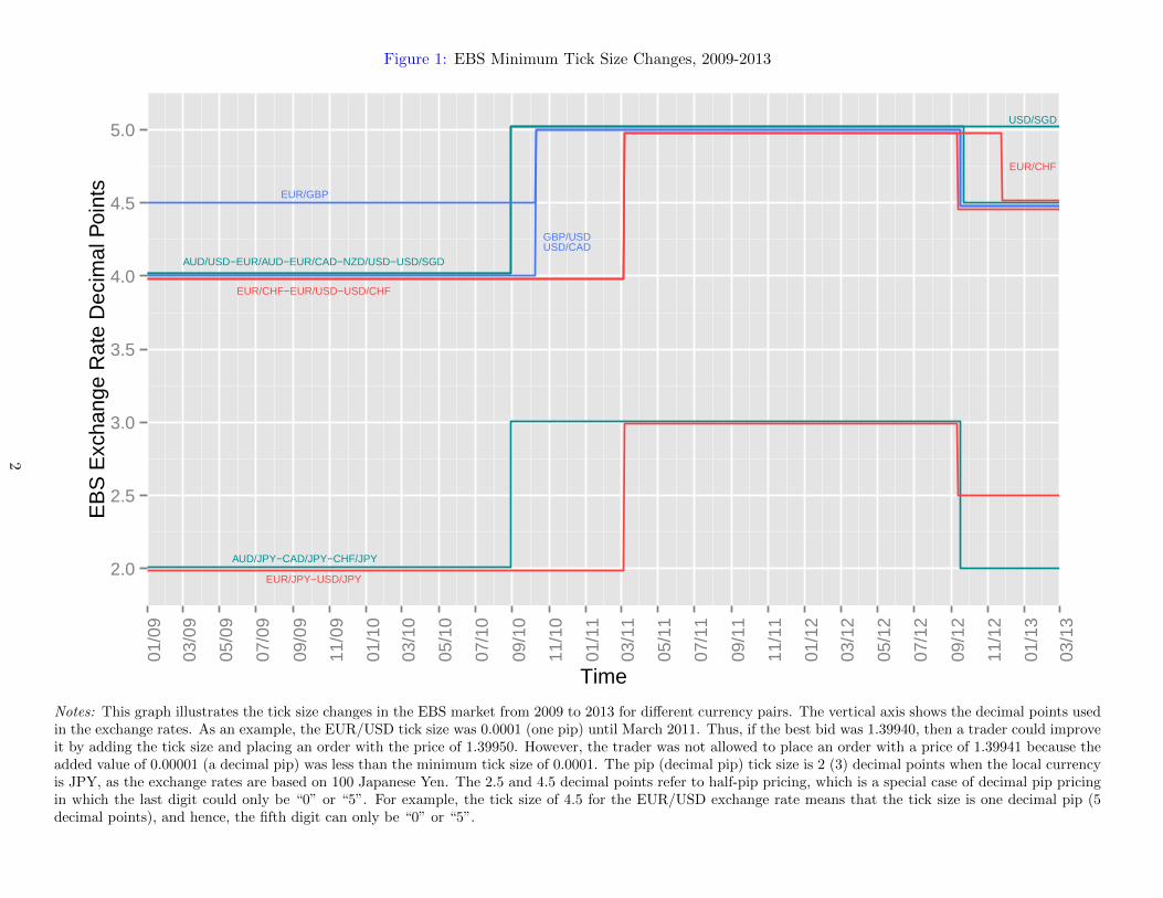
Figure 1: EBS Minimum Tick Size Changes, 2009-2013
AUD/USD−EUR/AUD−EUR/CAD−NZD/USD−USD/SGD
USD/SGD
AUD/JPY−CAD/JPY−CHF/JPY
GBP/USDUSD/CAD
EUR/GBP
EUR/CHF−EUR/USD−USD/CHF
EUR/CHF
EUR/JPY−USD/JPY2.0
2.5
3.0
3.5
4.0
4.5
5.001
/09
03/0
9
05/0
9
07/0
9
09/0
9
11/0
9
01/1
0
03/1
0
05/1
0
07/1
0
09/1
0
11/1
0
01/1
1
03/1
1
05/1
1
07/1
1
09/1
1
11/1
1
01/1
2
03/1
2
05/1
2
07/1
2
09/1
2
11/1
2
01/1
3
03/1
3
Time
EB
S E
xcha
nge
Rat
e D
ecim
al P
oint
s
Notes: This graph illustrates the tick size changes in the EBS market from 2009 to 2013 for different currency pairs. The vertical axis shows the decimal points usedin the exchange rates. As an example, the EUR/USD tick size was 0.0001 (one pip) until March 2011. Thus, if the best bid was 1.39940, then a trader could improveit by adding the tick size and placing an order with the price of 1.39950. However, the trader was not allowed to place an order with a price of 1.39941 because theadded value of 0.00001 (a decimal pip) was less than the minimum tick size of 0.0001. The pip (decimal pip) tick size is 2 (3) decimal points when the local currencyis JPY, as the exchange rates are based on 100 Japanese Yen. The 2.5 and 4.5 decimal points refer to half-pip pricing, which is a special case of decimal pip pricingin which the last digit could only be “0” or “5”. For example, the tick size of 4.5 for the EUR/USD exchange rate means that the tick size is one decimal pip (5decimal points), and hence, the fifth digit can only be “0” or “5”.
2
We study how the structure of the EBS market permitted HFTs to implement the sub-penny
jumping strategy to take advantage of the lower tick size.3 In the EBS market, manual traders
usually place large orders and do not cancel them very often. HFTs use this information by trading
in front and on the same side of the manual traders by improving the price by the smallest possible
amount (the tick size). We call this quote matching strategy sub-penny jumping.4 Sub-penny
jumpers try to extract the option values of the manual traders’ orders. Once a sub-penny jumper
(these traders are HFTs) trades in front of a manual trader, he is protected from serious losses on
his position because in the event of an adverse price movement, the sub-penny jumper limits his
losses by trading with the manual trader. However, if there is a favorable price move, the sub-
penny jumper profits to the full extent of the price changes. Therefore, the gains of the sub-penny
jumper may be unlimited on the upside and bounded on the downside. The sub-penny jumper
profits at the expense of the manual trader by taking liquidity that otherwise would have gone to
the manual trader. In addition to sub-penny jumping, order anticipation strategies are also used
for front-running by HFTs.
Then, we discuss the effects of the tick size change on spreads, market depths and arbitrage op-
portunities. Using the difference-in-difference estimators, we find that as a measure of the liquidity
cost, the spread becomes smaller after the introduction of decimal pip pricing. However, we argue
that due to the implementation of the sub-penny jumping strategy by HFTs, manual traders would
be pushed back in the limit order book and face higher spreads compared to HFTs. Therefore, the
spread is not a sufficient criterion for market quality after the tick size change. The analysis of the
limit order book indicates that the market depth decreased after the tick size change. Liquidity
providers prefer depth because there will be a sufficient volume of pending orders, preventing a
large order from significantly moving the price. We also find that there was no strong difference in
the number of arbitrage opportunities before and after the tick size change.
The remainder of the paper is organized as follows: Section 2 provides a brief literature re-
view, Section 3 describes the data and the EBS market, Section 4 presents sub-penny jumping, Sec-
tion 5 provides empirical evidence for the existence of sub-penny jumping, Section 6 discusses the
effect of the tick size reduction on market quality, and Section 7 concludes.
3Sub-penny jumping is a type of front-running strategy in which the sub-penny jumper trades in front and on thesame side of a large, patient trader.
4Quote matching has been called penny jumping after using the decimal format since 2001 in U.S. security markets.We use the term “sub-penny jumping” because the tick size is smaller than a penny in the EBS market.
3

2. Literature Review
There are only a few papers that study the tick size change in the interbank foreign exchange
market. Using confidential data from EBS, Schmidt (2012) documents that manual traders did not
use decimal pip pricing very often after the tick size change. He also provides the taxonomy of the
types of EBS customers and their order placement features. Lallouache and Frederic (2014) analyze
the data distributions of EUR/USD and USD/JPY and report the price clustering at prices ending
in “0” and “5” after March 2011. They argue that “automated” traders take price priority by
submitting limit orders one tick ahead of clusters. However, they do not provide insight as to why
these traders take such a priority. The common observation that emerges from these two papers is
that the EBS market’s microstructure changed significantly after the introduction of decimal pip
pricing. However, the reasons for this change and the consequences remain unresolved.
The literature on the tick size change in security markets is controversial with respect to the
effects of the tick size change. Bessembinder (2000) finds that spreads are reduced when the tick
size is lower. The findings of Jones and Lipson (2001) and Goldstein and Kavajecz (2000) reveal
that the spread is not a sufficient criterion for market quality. Bessembinder (2003) finds that both
spreads and intraday return volatility decreased after decimalization. The reduction for quoted
spreads was stronger in the heavily traded large-capitalization NASDAQ stocks. On the Kuala
Lumpur Stock Exchange, where the tick size increases with the price, Chung et al. (2005) find that
stocks that are subject to greater tick sizes have wider spreads and less quote clustering. Bourghelle
and Declerck (2004) show that the tick size change generated neither a lower liquidity provision
for large trades nor a change in the spread on the Paris Bourse Ahn et al. (2007) find that the
spread declined significantly after the Tokyo Stock Exchange (TSE) introduced a change in tick
sizes for stocks traded within certain price ranges. Reductions in spreads are larger for stocks with
larger tick size reductions and higher trading activity. Bacidore et al. (2001) show that the quoting
intensity and cancellation rates of limit orders increased after switching to decimal pricing. Chung
and Chuwonganant (2002) discover that the number of quote revisions increased dramatically after
the minimum tick size reduction. Lastly, Cai et al. (2008) conclude that there is no general effect
of a tick size reduction on the TSE because the trading volume, the number of shares traded, and
the average trade size react differently.5
5The controversies have led to theoretical studies about the choice of a suitable minimum tick size, Harris (1994),Anshuman and Kalay (1998), Cordella and Foucault (1999), Alexander and Zabotina (2005), Kadan (2006), andAscioglu et al. (2010).
4
3. Data Description and Market Structure
Banks usually trade currencies with each other on two wholesale electronic trading platforms,
namely, EBS and Thomson Reuters. The decision whether to use EBS or Reuters is usually driven
by the currency pair. In practice, EBS is the leading liquidity provider for EUR/USD, USD/JPY,
EUR/JPY, USD/CHF and EUR/CHF, and Reuters is the primary trading venue for commonwealth
and emerging market currencies. The data set used in this study is the EBS level 5 limit order
book, which includes 10 levels of “Quotes” (buy, sell) and “Deal” records at 100 milliseconds each.
Orders are submitted in units of millions of the base currency. Currently, the available transaction
data provided by EBS do not have dealer identifications or characteristics. To analyze the effect of
the minimum tick size change in March 2011, we have chosen the data from May 2011 to October
2011, as the share of the EBS customers using decimal pips mostly stabilized starting in May
2011. We excluded thin weekend trading periods and holidays because the liquidity may have been
extremely limited. We controlled for daylight savings time (summer) and standard time (winter).
Similar conventions were adopted by Andersen et al. (2003) and Chaboud et al. (2004).
In this section, we provide information about the EBS market. We explain the structure of the
EBS market and our analysis, which is based on the EUR/USD currency pair. The other major
currency pairs USD/JPY, USD/CHF, EUR/CHF, and EUR/JPY are mostly similar to EUR/USD.6 We
will discuss the distribution of the EBS customers, their fill ratio, the volume distribution and their
reactions to the introduction of decimal pip pricing. The information in this section is necessary to
gain an understanding of our analysis of the sub-penny jumping strategy, which we believe changed
the EBS market’s microstructure.
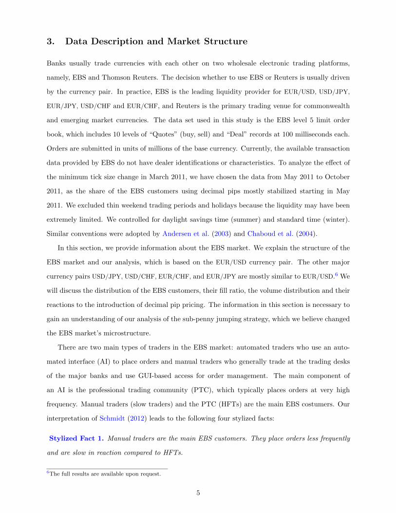
There are two main types of traders in the EBS market: automated traders who use an auto-
mated interface (AI) to place orders and manual traders who generally trade at the trading desks
of the major banks and use GUI-based access for order management. The main component of
an AI is the professional trading community (PTC), which typically places orders at very high
frequency. Manual traders (slow traders) and the PTC (HFTs) are the main EBS costumers. Our
interpretation of Schmidt (2012) leads to the following four stylized facts:
Stylized Fact 1. Manual traders are the main EBS customers. They place orders less frequently
and are slow in reaction compared to HFTs.
6The full results are available upon request.
5
Manual traders compose approximately 75% of all EBS costumers in EUR/USD, for example,
whereas the PTC comprises 16.6% of the customers for the same currency pair. Although manual
traders are the main EBS costumers, they place only 3.7% of the daily orders for EUR/USD, and
the PTC places 61.6% of all orders.
Stylized Fact 2. Manual traders typically place large orders in the order book, whereas HFTs
place smaller orders.
Comparisons of the order sizes reveal that the PTC typically uses an order size of one million
and almost never uses an order size exceeding four million for the EUR/USD currency pair. In
contrast, manual traders place large orders, for example, approximately 5% of the orders submitted
by manual traders reach the size of ten million. Such separation in the order sizes permits us to
identify the manual traders and the PTC.
Stylized Fact 3. Manual traders do not typically cancel their orders, which is in contrast to
HFTs; therefore, manual traders have a high fill ratio.
The fill ratio is defined as the ratio of the dealt quotes to the submitted quotes. This ratio
is more than 50% for the manual traders and approximately 7% for the PTC. The high fill ratio
for the manual traders means that they typically do not cancel their orders, whereas the HFTs do
cancel more often, leading to their low fill ratio. All EBS costumers should meet the minimum fill
ratio of 3% since July 2012.
Stylized Fact 4. Manual traders usually place orders at prices ending in “0”.
In the period under study, manual traders did not widely use decimal pip pricing. Approximately
80% of the manual traders used decimal pip pricing in less than 20% of their orders. Simultaneously,
less than 2% of manual traders used decimal pips for more than 80% of their orders. In contrast,
AI traders have adopted decimal pip pricing very well: more than 50% of AI traders used decimal
pip pricing in more than 80% percent of their orders, and approximately12% of them used decimal
pips in less than 20% of their orders.
The following statement is our first hypothesis regarding the manual traders’ order placement
strategy.
Hypothesis 1. Manual traders typically place large orders at prices ending in “0” and do not
cancel their orders very often.
6
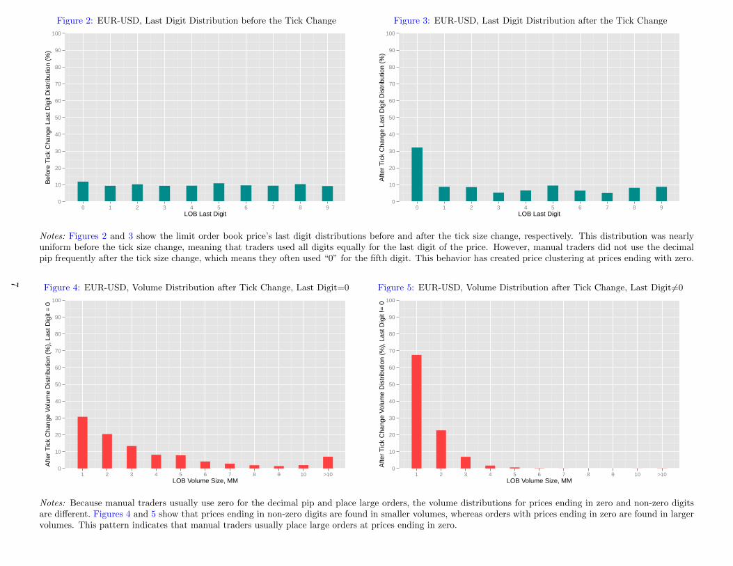
Figure 2: EUR-USD, Last Digit Distribution before the Tick Change
0
10
20
30
40
50
60
70
80
90
100
0 1 2 3 4 5 6 7 8 9LOB Last Digit
Bef
ore
Tic
k C
hang
e La
st D
igit
Dis
trib
utio
n (%
)
Figure 3: EUR-USD, Last Digit Distribution after the Tick Change
0
10
20
30
40
50
60
70
80
90
100
0 1 2 3 4 5 6 7 8 9LOB Last Digit
Afte
r T
ick
Cha
nge
Last
Dig
it D
istr
ibut
ion
(%)
Notes: Figures 2 and 3 show the limit order book price’s last digit distributions before and after the tick size change, respectively. This distribution was nearlyuniform before the tick size change, meaning that traders used all digits equally for the last digit of the price. However, manual traders did not use the decimalpip frequently after the tick size change, which means they often used “0” for the fifth digit. This behavior has created price clustering at prices ending with zero.
Figure 4: EUR-USD, Volume Distribution after Tick Change, Last Digit=0
0
10
20
30
40
50
60
70
80
90
100
1 2 3 4 5 6 7 8 9 10 >10LOB Volume Size, MM
Afte
r T
ick
Cha
nge
Vol
ume
Dis
trib
utio
n (%
), L
ast D
igit
= 0
Figure 5: EUR-USD, Volume Distribution after Tick Change, Last Digit6=0
0
10
20
30
40
50
60
70
80
90
100
1 2 3 4 5 6 7 8 9 10 >10LOB Volume Size, MM
Afte
r T
ick
Cha
nge
Vol
ume
Dis
trib
utio
n (%
), L
ast D
igit
!= 0
Notes: Because manual traders usually use zero for the decimal pip and place large orders, the volume distributions for prices ending in zero and non-zero digitsare different. Figures 4 and 5 show that prices ending in non-zero digits are found in smaller volumes, whereas orders with prices ending in zero are found in largervolumes. This pattern indicates that manual traders usually place large orders at prices ending in zero.
7
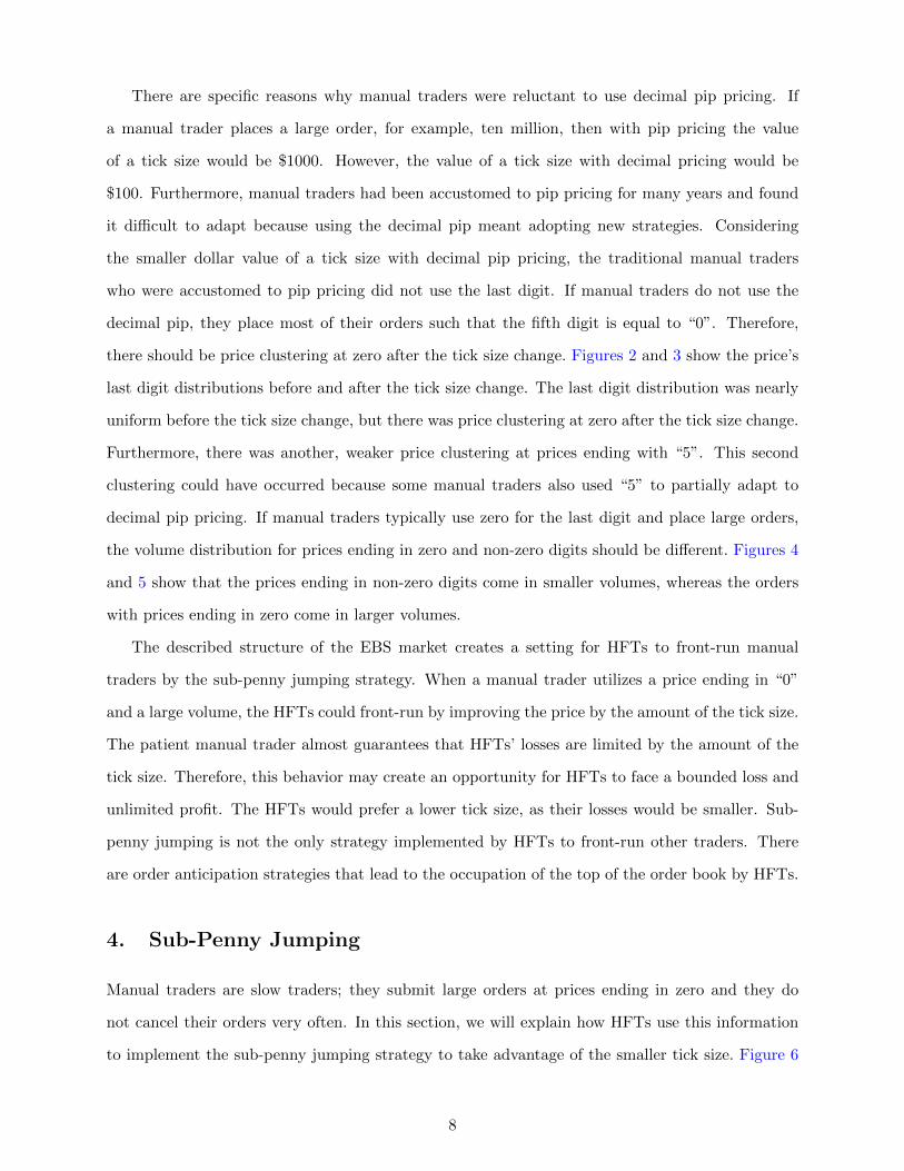
There are specific reasons why manual traders were reluctant to use decimal pip pricing. If
a manual trader places a large order, for example, ten million, then with pip pricing the value
of a tick size would be $1000. However, the value of a tick size with decimal pricing would be
$100. Furthermore, manual traders had been accustomed to pip pricing for many years and found
it difficult to adapt because using the decimal pip meant adopting new strategies. Considering
the smaller dollar value of a tick size with decimal pip pricing, the traditional manual traders
who were accustomed to pip pricing did not use the last digit. If manual traders do not use the
decimal pip, they place most of their orders such that the fifth digit is equal to “0”. Therefore,
there should be price clustering at zero after the tick size change. Figures 2 and 3 show the price’s
last digit distributions before and after the tick size change. The last digit distribution was nearly
uniform before the tick size change, but there was price clustering at zero after the tick size change.
Furthermore, there was another, weaker price clustering at prices ending with “5”. This second
clustering could have occurred because some manual traders also used “5” to partially adapt to
decimal pip pricing. If manual traders typically use zero for the last digit and place large orders,
the volume distribution for prices ending in zero and non-zero digits should be different. Figures 4
and 5 show that the prices ending in non-zero digits come in smaller volumes, whereas the orders
with prices ending in zero come in larger volumes.
The described structure of the EBS market creates a setting for HFTs to front-run manual
traders by the sub-penny jumping strategy. When a manual trader utilizes a price ending in “0”
and a large volume, the HFTs could front-run by improving the price by the amount of the tick size.
The patient manual trader almost guarantees that HFTs’ losses are limited by the amount of the
tick size. Therefore, this behavior may create an opportunity for HFTs to face a bounded loss and
unlimited profit. The HFTs would prefer a lower tick size, as their losses would be smaller. Sub-
penny jumping is not the only strategy implemented by HFTs to front-run other traders. There
are order anticipation strategies that lead to the occupation of the top of the order book by HFTs.
4. Sub-Penny Jumping
Manual traders are slow traders; they submit large orders at prices ending in zero and they do
not cancel their orders very often. In this section, we will explain how HFTs use this information
to implement the sub-penny jumping strategy to take advantage of the smaller tick size. Figure 6
8
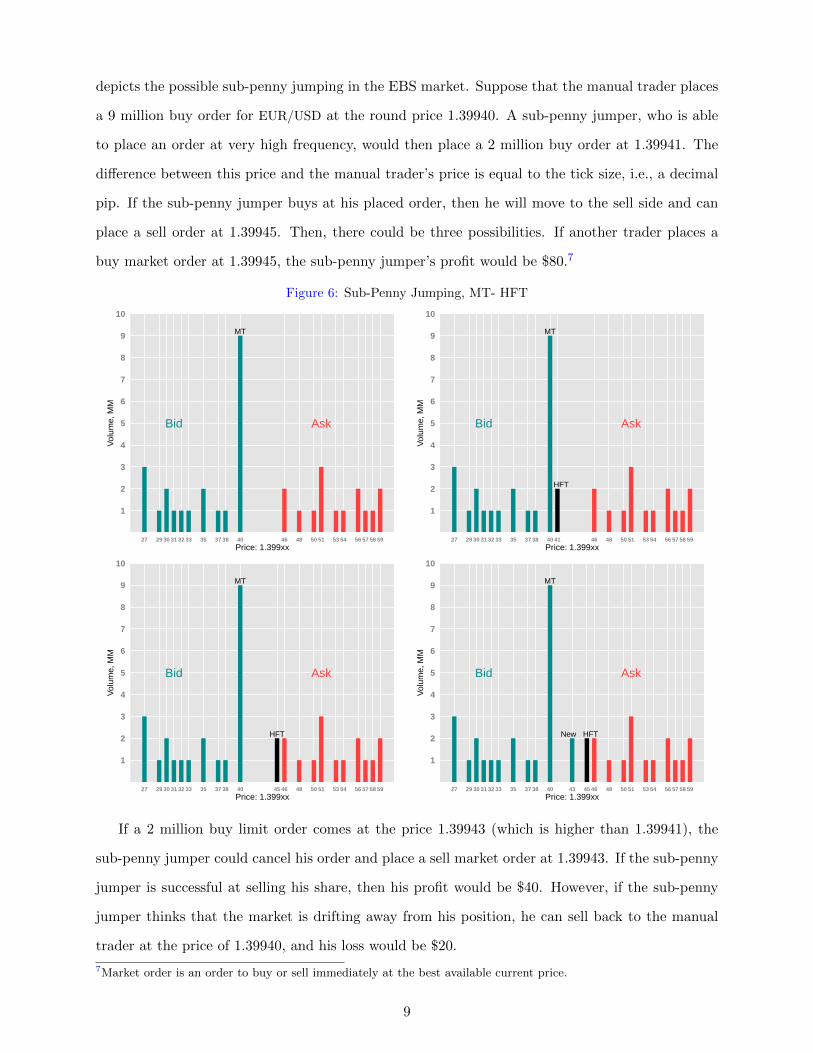
depicts the possible sub-penny jumping in the EBS market. Suppose that the manual trader places
a 9 million buy order for EUR/USD at the round price 1.39940. A sub-penny jumper, who is able
to place an order at very high frequency, would then place a 2 million buy order at 1.39941. The
difference between this price and the manual trader’s price is equal to the tick size, i.e., a decimal
pip. If the sub-penny jumper buys at his placed order, then he will move to the sell side and can
place a sell order at 1.39945. Then, there could be three possibilities. If another trader places a
buy market order at 1.39945, the sub-penny jumper’s profit would be $80.7
Figure 6: Sub-Penny Jumping, MT- HFT
Bid Ask
MT
1
2
3
4
5
6
7
8
9
10
27 29 30 31 32 33 35 37 38 40 46 48 50 51 53 54 56 57 58 59
Price: 1.399xx
Vol
ume,
MM
Bid Ask
MT
HFT
1
2
3
4
5
6
7
8
9
10
27 29 30 31 32 33 35 37 38 40 41 46 48 50 51 53 54 56 57 58 59
Price: 1.399xx
Vol
ume,
MM
Bid Ask
MT
HFT
1
2
3
4
5
6
7
8
9
10
27 29 30 31 32 33 35 37 38 40 45 46 48 50 51 53 54 56 57 58 59
Price: 1.399xx
Vol
ume,
MM
Bid Ask
MT
New HFT
1
2
3
4
5
6
7
8
9
10
27 29 30 31 32 33 35 37 38 40 43 45 46 48 50 51 53 54 56 57 58 59
Price: 1.399xx
Vol
ume,
MM
If a 2 million buy limit order comes at the price 1.39943 (which is higher than 1.39941), the
sub-penny jumper could cancel his order and place a sell market order at 1.39943. If the sub-penny
jumper is successful at selling his share, then his profit would be $40. However, if the sub-penny
jumper thinks that the market is drifting away from his position, he can sell back to the manual
trader at the price of 1.39940, and his loss would be $20.
7Market order is an order to buy or sell immediately at the best available current price.
9
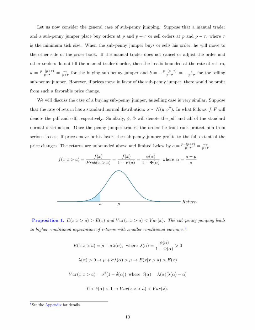
Let us now consider the general case of sub-penny jumping. Suppose that a manual trader
and a sub-penny jumper place buy orders at p and p + τ or sell orders at p and p − τ , where τ
is the minimum tick size. When the sub-penny jumper buys or sells his order, he will move to
the other side of the order book. If the manual trader does not cancel or adjust the order and
other traders do not fill the manual trader’s order, then the loss is bounded at the rate of return,
a = p−(p+τ)p+τ = −τ
p+τ for the buying sub-penny jumper and b = −p−(p−τ)p−τ = − τ
p−τ for the selling
sub-penny jumper. However, if prices move in favor of the sub-penny jumper, there would be profit
from such a favorable price change.
We will discuss the case of a buying sub-penny jumper, as selling case is very similar. Suppose
that the rate of return has a standard normal distribution: x ∼ N(µ, σ2). In what follows, f, F will
denote the pdf and cdf, respectively. Similarly, φ, Φ will denote the pdf and cdf of the standard
normal distribution. Once the penny jumper trades, the orders he front-runs protect him from
serious losses. If prices move in his favor, the sub-penny jumper profits to the full extent of the
price changes. The returns are unbounded above and limited below by a = p−(p+τ)p+τ = −τ
p+τ .
f(x|x > a) =f(x)
Prob(x > a)=
f(x)
1− F (a)=
φ(α)
1− Φ(α)where α =
a− µσ
µa Return
Proposition 1. E(x|x > a) > E(x) and V ar(x|x > a) < V ar(x). The sub-penny jumping leads
to higher conditional expectation of returns with smaller conditional variance.8
E(x|x > a) = µ+ σλ(α), where λ(α) =φ(α)
1− Φ(α)> 0
λ(α) > 0→ µ+ σλ(α) > µ→ E(x|x > a) > E(x)
V ar(x|x > a) = σ2(1− δ(α)) where δ(α) = λ(α)[λ(α)− α]
0 < δ(α) < 1→ V ar(x|x > a) < V ar(x).
8See the Appendix for details.
10
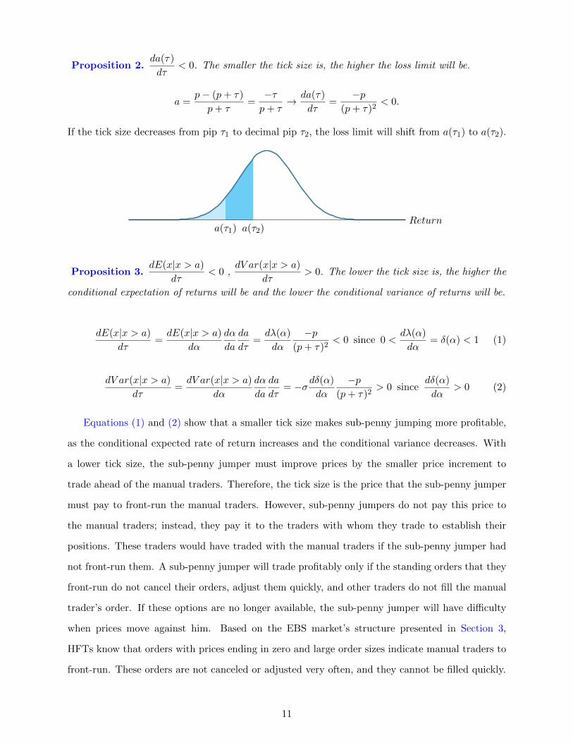
Proposition 2.da(τ)
dτ< 0. The smaller the tick size is, the higher the loss limit will be.
a =p− (p+ τ)
p+ τ=−τp+ τ
→ da(τ)
dτ=
−p(p+ τ)2
< 0.
If the tick size decreases from pip τ1 to decimal pip τ2, the loss limit will shift from a(τ1) to a(τ2).
a(τ2)a(τ1)Return
Proposition 3.dE(x|x > a)
dτ< 0 ,
dV ar(x|x > a)
dτ> 0. The lower the tick size is, the higher the
conditional expectation of returns will be and the lower the conditional variance of returns will be.
dE(x|x > a)
dτ=dE(x|x > a)
dα
dα
da
da
dτ=dλ(α)
dα
−p(p+ τ)2
< 0 since 0 <dλ(α)
dα= δ(α) < 1 (1)
dV ar(x|x > a)
dτ=dV ar(x|x > a)
dα
dα
da
da
dτ= −σdδ(α)
dα
−p(p+ τ)2
> 0 sincedδ(α)
dα> 0 (2)
Equations (1) and (2) show that a smaller tick size makes sub-penny jumping more profitable,
as the conditional expected rate of return increases and the conditional variance decreases. With
a lower tick size, the sub-penny jumper must improve prices by the smaller price increment to
trade ahead of the manual traders. Therefore, the tick size is the price that the sub-penny jumper
must pay to front-run the manual traders. However, sub-penny jumpers do not pay this price to
the manual traders; instead, they pay it to the traders with whom they trade to establish their
positions. These traders would have traded with the manual traders if the sub-penny jumper had
not front-run them. A sub-penny jumper will trade profitably only if the standing orders that they
front-run do not cancel their orders, adjust them quickly, and other traders do not fill the manual
trader’s order. If these options are no longer available, the sub-penny jumper will have difficulty
when prices move against him. Based on the EBS market’s structure presented in Section 3,
HFTs know that orders with prices ending in zero and large order sizes indicate manual traders to
front-run. These orders are not canceled or adjusted very often, and they cannot be filled quickly.
11
5. Sub-Penny Jumping, Deal and Quote Distributions
Because manual traders were reluctant to use decimal pip pricing, there is a price clustering of
quotes in all limit order book levels at prices ending in zero. Furthermore, if a buying manual
trader places an order with a price ending with “0” (e.g., 1.39940), then the buying sub-penny
jumper who wants to front-run the manual trader should place an order with a price ending with
“1” (1.39941). If there are other sub-penny jumpers, they would place their orders with prices
ending with “2”, “3” and etc. However, greater distance from “0” means less expected profit;
therefore, we would expect a decreasing distribution of the number of orders for the buy side of
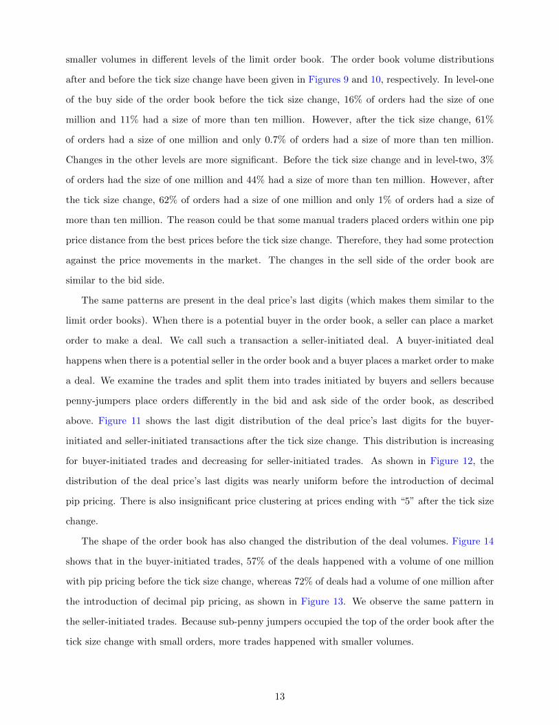
the limit order book in all levels. Figure 7 shows such distributions for the ten levels of the order
book with different last digits. For example, at the level-one buy side of the limit order book, 28%
of orders have the last digit “0” and only approximately 2.5% of the orders have the last digit “9”.
The shape of the distributions in other levels of the bid side are similar to the shape of the level-one
distribution.
If a sub-penny jumper improves upon the order of a manual trader by one tick while bidding, he
would place an order with the last digit of “1”. However, if the HFT improves the manual trader’s
price (e.g., 1.39940) on the ask side, he should place a price ending with “9” (1.39939). Therefore,
we would expect an increasing distribution (excluding “0”) for all levels of the sell side of the limit
order book. For example, from Figure 7 we see that approximately 28% of the orders have the last
digit “0”, but only approximately 2.7% of the orders have the last digit “1”. This ratio starts to
rise and reaches 19.5% for orders with the last digit “9”. The shape of the distributions in other
levels of the ask side are similar to the shape of the level-one distribution. As shown in Figure 8,
the distributions of orders were almost uniform before the tick size change for both the bid and ask
sides. Distributions after the tick size change also show weaker price clustering at prices ending
with “5”. It seems that some manual traders placed such orders to adopt decimal pip pricing
partially without the complexity of using all digits. However, the volume sizes used with this digit
are small and there was no opportunity for HFTs to front-run the digit “5”.
Volume distributions also give us information about the consequences of the sub-penny jumping
strategy in the limit order book. When HFTs front-run manual traders, they secure their positions
by placing orders of smaller volumes. We know from Section 3 that HFTs typically use one million
orders and almost never use an order size exceeding four million. As a result, we should observe
12
smaller volumes in different levels of the limit order book. The order book volume distributions
after and before the tick size change have been given in Figures 9 and 10, respectively. In level-one
of the buy side of the order book before the tick size change, 16% of orders had the size of one
million and 11% had a size of more than ten million. However, after the tick size change, 61%
of orders had a size of one million and only 0.7% of orders had a size of more than ten million.
Changes in the other levels are more significant. Before the tick size change and in level-two, 3%
of orders had the size of one million and 44% had a size of more than ten million. However, after
the tick size change, 62% of orders had a size of one million and only 1% of orders had a size of
more than ten million. The reason could be that some manual traders placed orders within one pip
price distance from the best prices before the tick size change. Therefore, they had some protection
against the price movements in the market. The changes in the sell side of the order book are
similar to the bid side.
The same patterns are present in the deal price’s last digits (which makes them similar to the
limit order books). When there is a potential buyer in the order book, a seller can place a market
order to make a deal. We call such a transaction a seller-initiated deal. A buyer-initiated deal
happens when there is a potential seller in the order book and a buyer places a market order to make
a deal. We examine the trades and split them into trades initiated by buyers and sellers because
penny-jumpers place orders differently in the bid and ask side of the order book, as described
above. Figure 11 shows the last digit distribution of the deal price’s last digits for the buyer-
initiated and seller-initiated transactions after the tick size change. This distribution is increasing
for buyer-initiated trades and decreasing for seller-initiated trades. As shown in Figure 12, the
distribution of the deal price’s last digits was nearly uniform before the introduction of decimal
pip pricing. There is also insignificant price clustering at prices ending with “5” after the tick size
change.
The shape of the order book has also changed the distribution of the deal volumes. Figure 14
shows that in the buyer-initiated trades, 57% of the deals happened with a volume of one million
with pip pricing before the tick size change, whereas 72% of deals had a volume of one million after
the introduction of decimal pip pricing, as shown in Figure 13. We observe the same pattern in
the seller-initiated trades. Because sub-penny jumpers occupied the top of the order book after the
tick size change with small orders, more trades happened with smaller volumes.
13
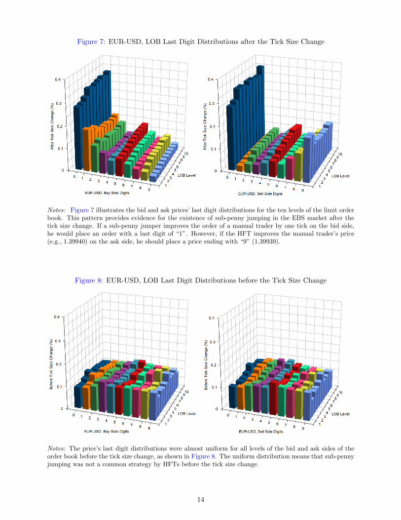
Figure 7: EUR-USD, LOB Last Digit Distributions after the Tick Size Change
Notes: Figure 7 illustrates the bid and ask prices’ last digit distributions for the ten levels of the limit orderbook. This pattern provides evidence for the existence of sub-penny jumping in the EBS market after thetick size change. If a sub-penny jumper improves the order of a manual trader by one tick on the bid side,he would place an order with a last digit of “1”. However, if the HFT improves the manual trader’s price(e.g., 1.39940) on the ask side, he should place a price ending with “9” (1.39939).
Figure 8: EUR-USD, LOB Last Digit Distributions before the Tick Size Change
Notes: The price’s last digit distributions were almost uniform for all levels of the bid and ask sides of theorder book before the tick size change, as shown in Figure 8. The uniform distribution means that sub-pennyjumping was not a common strategy by HFTs before the tick size change.
14
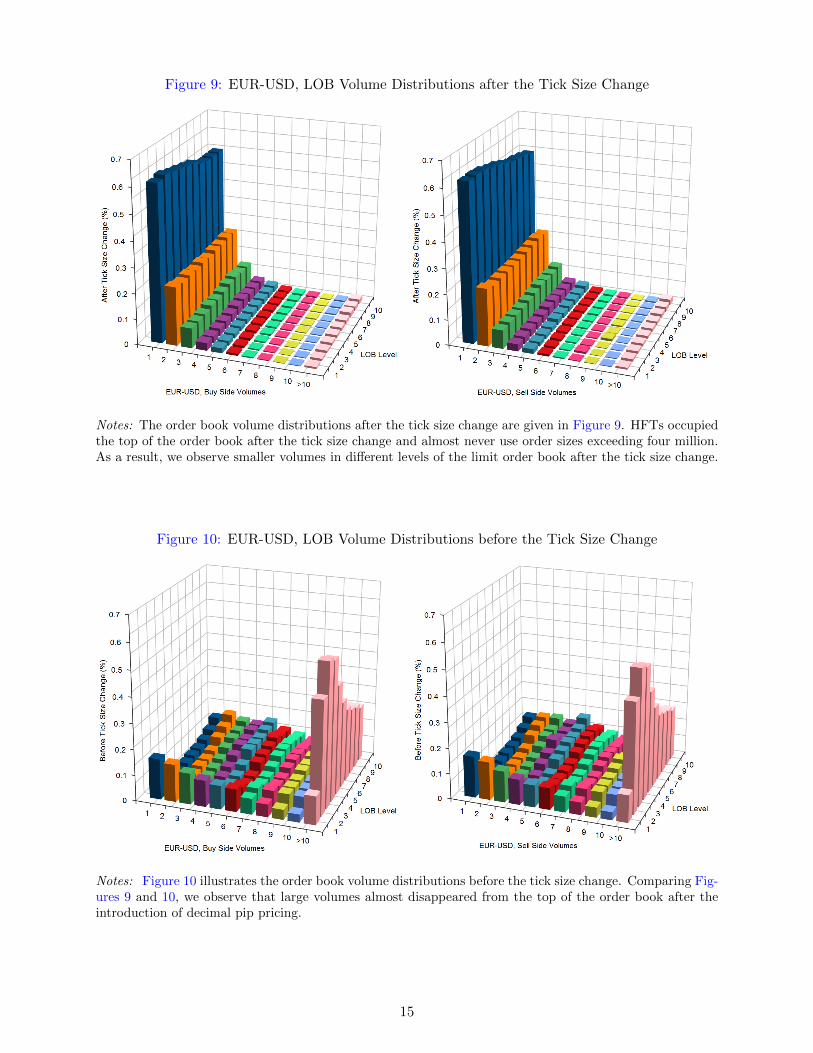
Figure 9: EUR-USD, LOB Volume Distributions after the Tick Size Change
Notes: The order book volume distributions after the tick size change are given in Figure 9. HFTs occupiedthe top of the order book after the tick size change and almost never use order sizes exceeding four million.As a result, we observe smaller volumes in different levels of the limit order book after the tick size change.
Figure 10: EUR-USD, LOB Volume Distributions before the Tick Size Change
Notes: Figure 10 illustrates the order book volume distributions before the tick size change. Comparing Fig-ures 9 and 10, we observe that large volumes almost disappeared from the top of the order book after theintroduction of decimal pip pricing.
15
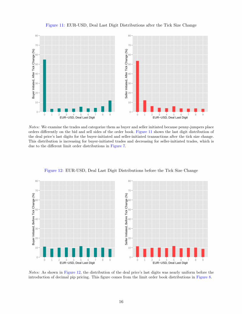
Figure 11: EUR-USD, Deal Last Digit Distributions after the Tick Size Change
0
10
20
30
40
50
60
70
80
0 1 2 3 4 5 6 7 8 9EUR−USD, Deal Last Digit
Buy
er In
itiat
ed, A
fter
Tic
k C
hang
e (%
)
0
10
20
30
40
50
60
70
80
0 1 2 3 4 5 6 7 8 9EUR−USD, Deal Last Digit
Sel
ler
Initi
ated
, Afte
r T
ick
Cha
nge
(%)
Notes: We examine the trades and categorize them as buyer and seller initiated because penny-jumpers placeorders differently on the bid and sell sides of the order book. Figure 11 shows the last digit distribution ofthe deal price’s last digits for the buyer-initiated and seller-initiated transactions after the tick size change.This distribution is increasing for buyer-initiated trades and decreasing for seller-initiated trades, which isdue to the different limit order distributions in Figure 7.
Figure 12: EUR-USD, Deal Last Digit Distributions before the Tick Size Change
0
10
20
30
40
50
60
70
80
0 1 2 3 4 5 6 7 8 9EUR−USD, Deal Last Digit
Buy
er In
itiat
ed, B
efor
e T
ick
Cha
nge
(%)
0
10
20
30
40
50
60
70
80
0 1 2 3 4 5 6 7 8 9EUR−USD, Deal Last Digit
Sel
ler
Initi
ated
, Bef
ore
Tic
k C
hang
e (%
)
Notes: As shown in Figure 12, the distribution of the deal price’s last digits was nearly uniform before theintroduction of decimal pip pricing. This figure comes from the limit order book distributions in Figure 8.
16
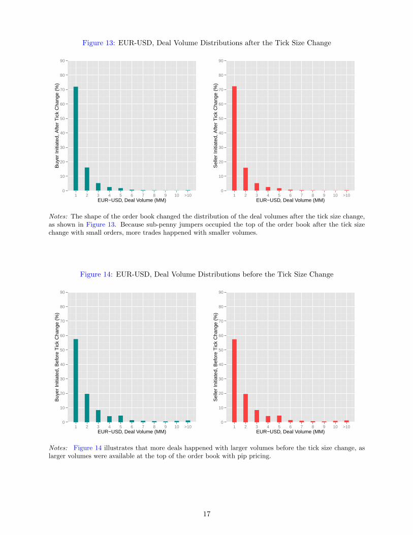
Figure 13: EUR-USD, Deal Volume Distributions after the Tick Size Change
0
10
20
30
40
50
60
70
80
90
1 2 3 4 5 6 7 8 9 10 >10EUR−USD, Deal Volume (MM)
Buy
er In
itiat
ed, A
fter
Tic
k C
hang
e (%
)
0
10
20
30
40
50
60
70
80
90
1 2 3 4 5 6 7 8 9 10 >10EUR−USD, Deal Volume (MM)
Sel
ler
Initi
ated
, Afte
r T
ick
Cha
nge
(%)
Notes: The shape of the order book changed the distribution of the deal volumes after the tick size change,as shown in Figure 13. Because sub-penny jumpers occupied the top of the order book after the tick sizechange with small orders, more trades happened with smaller volumes.
Figure 14: EUR-USD, Deal Volume Distributions before the Tick Size Change
0
10
20
30
40
50
60
70
80
90
1 2 3 4 5 6 7 8 9 10 >10EUR−USD, Deal Volume (MM)
Buy
er In
itiat
ed, B
efor
e T
ick
Cha
nge
(%)
0
10
20
30
40
50
60
70
80
90
1 2 3 4 5 6 7 8 9 10 >10EUR−USD, Deal Volume (MM)
Sel
ler
Initi
ated
, Bef
ore
Tic
k C
hang
e (%
)
Notes: Figure 14 illustrates that more deals happened with larger volumes before the tick size change, aslarger volumes were available at the top of the order book with pip pricing.
17
6. The Effects of the Lower Tick Size on Market Quality
6.1. Spread
Spread is one of the measures of liquidity costs. Spread is defined as the difference between the
best bid and the best asking price in the limit order book. In this section, we study the effects of
introduction of decimal pip pricing on the spread. Figure 15 shows the one-hour frequency spread
of the EUR/USD exchange rates for 2011. In the graph, each dot is a one-hour average spread and
there are 24 observations in each day. We have excluded the weekend, holidays and negative or zero
spread.9 When EBS changed the tick size from pip pricing to decimal pip pricing in March 2011,
there was a significant draw down in the spread. Therefore, we will test the following hypothesis
regarding the spread:
Hypothesis 2. Decimal pip pricing made the bid-ask spread narrower in EBS market.
To test the effects of the lower tick size on the spread, we use difference-in-difference (DID)
estimation. DID is typically used to identify the effects of a specific policy intervention or treatment.
The idea behind the DID approach is that if an intervention has an effect, the difference between the
unaffected group (the control group) and the group directly affected by the intervention (treatment
group) should change after the policy intervention. Then, one compares the difference in outcomes
between the two groups before and after the intervention. We chose EUR/USD as the treatment
group. The best control group in our case would be the same currency pair in the Reuters market
on the condition that the spread for EUR/USD in Reuters was not affected by the tick size change in
the EBS market. Unfortunately, we do not have access to this data set. Our next best options for
the control group are the busiest non-major currency pairs in the EBS market, namely, EUR/GBP,
AUD/USD and GBP/USD. We chose the same number of days before March 2011 (before the tick
change) and after May 2011 (after the tick change). The share of the EBS customers using decimal
pip mostly stabilized starting in May 2011. Our selected control groups were not affected directly by
the tick size change, as the tick size did not change for these currency pairs in the time span under
consideration. Moreover, we have not found any evidence that the control groups were affected
even indirectly by this change; if they were, they could not be used as control groups.10
9If there is no bilateral credit between a buyer and a seller at the top of the limit order book, the trade does nothappen and the spread could be negative or zero.
10If the HFTs moved activities from the control groups to the treatments groups to implement sub-penny jumping,the control groups would have been affected indirectly by the tick size change. We checked the deals and the stateof the limit order book of these control groups and did not find significant changes from January 2011 to July 2011.
18
Assuming that the treatment effect is stationary over time, we define the DID model by
St = β0 + β1P + β2T + β3PT + εt (3)
where T is a binary treatment variable that is equal to one for the EUR/USD and zero for the
control group. P is the binary post-treatment indicator, and it is equal to one after the tick size
change and zero before the change. T controls for the permanent differences between the treatment
and control groups, and β2 should capture this variation. Similarly, P controls for trends common
to both the control and treatment groups, and β1 will capture this variation. The variation that
remains is captured by β3. Conditional means corresponding to the four combinations of T and P
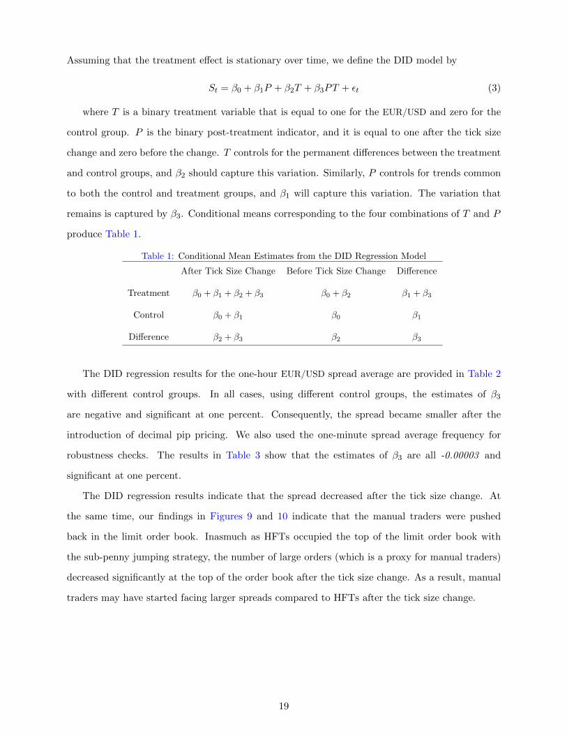
produce Table 1.
Table 1: Conditional Mean Estimates from the DID Regression Model
After Tick Size Change Before Tick Size Change Difference
Treatment β0 + β1 + β2 + β3 β0 + β2 β1 + β3
Control β0 + β1 β0 β1
Difference β2 + β3 β2 β3
The DID regression results for the one-hour EUR/USD spread average are provided in Table 2
with different control groups. In all cases, using different control groups, the estimates of β3
are negative and significant at one percent. Consequently, the spread became smaller after the
introduction of decimal pip pricing. We also used the one-minute spread average frequency for
robustness checks. The results in Table 3 show that the estimates of β3 are all -0.00003 and
significant at one percent.
The DID regression results indicate that the spread decreased after the tick size change. At
the same time, our findings in Figures 9 and 10 indicate that the manual traders were pushed
back in the limit order book. Inasmuch as HFTs occupied the top of the limit order book with
the sub-penny jumping strategy, the number of large orders (which is a proxy for manual traders)
decreased significantly at the top of the order book after the tick size change. As a result, manual
traders may have started facing larger spreads compared to HFTs after the tick size change.
19
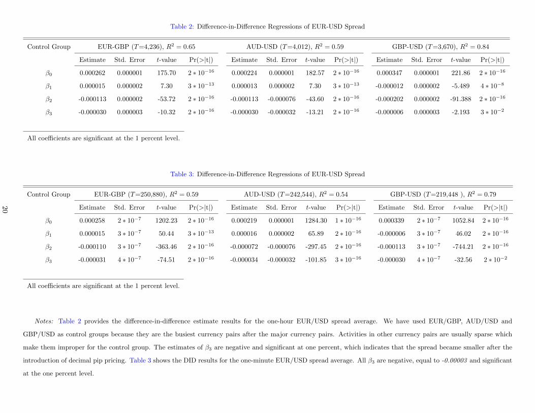
Table 2: Difference-in-Difference Regressions of EUR-USD Spread
Control Group EUR-GBP (T=4,236), R2 = 0.65 AUD-USD (T=4,012), R2 = 0.59 GBP-USD (T=3,670), R2 = 0.84
Estimate Std. Error t-value Pr(>|t|) Estimate Std. Error t-value Pr(>|t|) Estimate Std. Error t-value Pr(>|t|)
β0 0.000262 0.000001 175.70 2 ∗ 10−16 0.000224 0.000001 182.57 2 ∗ 10−16 0.000347 0.000001 221.86 2 ∗ 10−16
β1 0.000015 0.000002 7.30 3 ∗ 10−13 0.000013 0.000002 7.30 3 ∗ 10−13 -0.000012 0.000002 -5.489 4 ∗ 10−8
β2 -0.000113 0.000002 -53.72 2 ∗ 10−16 -0.000113 -0.000076 -43.60 2 ∗ 10−16 -0.000202 0.000002 -91.388 2 ∗ 10−16
β3 -0.000030 0.000003 -10.32 2 ∗ 10−16 -0.000030 -0.000032 -13.21 2 ∗ 10−16 -0.000006 0.000003 -2.193 3 ∗ 10−2
All coefficients are significant at the 1 percent level.
Table 3: Difference-in-Difference Regressions of EUR-USD Spread
Control Group EUR-GBP (T=250,880), R2 = 0.59 AUD-USD (T=242,544), R2 = 0.54 GBP-USD (T=219,448 ), R2 = 0.79
Estimate Std. Error t-value Pr(>|t|) Estimate Std. Error t-value Pr(>|t|) Estimate Std. Error t-value Pr(>|t|)
β0 0.000258 2 ∗ 10−7 1202.23 2 ∗ 10−16 0.000219 0.000001 1284.30 1 ∗ 10−16 0.000339 2 ∗ 10−7 1052.84 2 ∗ 10−16
β1 0.000015 3 ∗ 10−7 50.44 3 ∗ 10−13 0.000016 0.000002 65.89 2 ∗ 10−16 -0.000006 3 ∗ 10−7 46.02 2 ∗ 10−16
β2 -0.000110 3 ∗ 10−7 -363.46 2 ∗ 10−16 -0.000072 -0.000076 -297.45 2 ∗ 10−16 -0.000113 3 ∗ 10−7 -744.21 2 ∗ 10−16
β3 -0.000031 4 ∗ 10−7 -74.51 2 ∗ 10−16 -0.000034 -0.000032 -101.85 3 ∗ 10−16 -0.000030 4 ∗ 10−7 -32.56 2 ∗ 10−2
All coefficients are significant at the 1 percent level.
Notes: Table 2 provides the difference-in-difference estimate results for the one-hour EUR/USD spread average. We have used EUR/GBP, AUD/USD and
GBP/USD as control groups because they are the busiest currency pairs after the major currency pairs. Activities in other currency pairs are usually sparse which
make them improper for the control group. The estimates of β3 are negative and significant at one percent, which indicates that the spread became smaller after the
introduction of decimal pip pricing. Table 3 shows the DID results for the one-minute EUR/USD spread average. All β3 are negative, equal to -0.00003 and significant
at the one percent level.
20
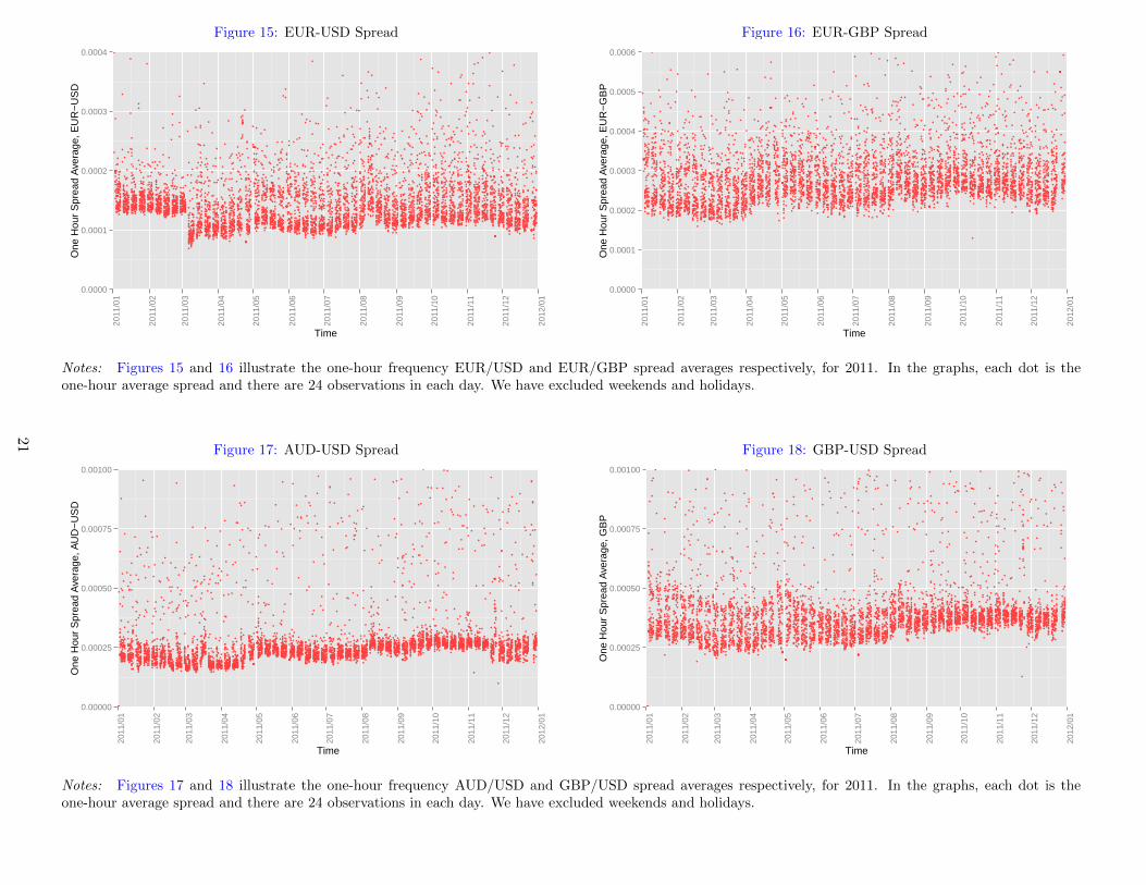
Figure 15: EUR-USD Spread
0.0000
0.0001
0.0002
0.0003
0.0004
2011
/01
2011
/02
2011
/03
2011
/04
2011
/05
2011
/06
2011
/07
2011
/08
2011
/09
2011
/10
2011
/11
2011
/12
2012
/01
Time
One
Hou
r S
prea
d A
vera
ge, E
UR
−U
SD
Figure 16: EUR-GBP Spread
0.0000
0.0001
0.0002
0.0003
0.0004
0.0005
0.0006
2011
/01
2011
/02
2011
/03
2011
/04
2011
/05
2011
/06
2011
/07
2011
/08
2011
/09
2011
/10
2011
/11
2011
/12
2012
/01
Time
One
Hou
r S
prea
d A
vera
ge, E
UR
−G
BP
Notes: Figures 15 and 16 illustrate the one-hour frequency EUR/USD and EUR/GBP spread averages respectively, for 2011. In the graphs, each dot is theone-hour average spread and there are 24 observations in each day. We have excluded weekends and holidays.
Figure 17: AUD-USD Spread
0.00000
0.00025
0.00050
0.00075
0.00100
2011
/01
2011
/02
2011
/03
2011
/04
2011
/05
2011
/06
2011
/07
2011
/08
2011
/09
2011
/10
2011
/11
2011
/12
2012
/01
Time
One
Hou
r S
prea
d A
vera
ge, A
UD
−U
SD
Figure 18: GBP-USD Spread
0.00000
0.00025
0.00050
0.00075
0.00100
2011
/01
2011
/02
2011
/03
2011
/04
2011
/05
2011
/06
2011
/07
2011
/08
2011
/09
2011
/10
2011
/11
2011
/12
2012
/01
Time
One
Hou
r S
prea
d A
vera
ge, G
BP
Notes: Figures 17 and 18 illustrate the one-hour frequency AUD/USD and GBP/USD spread averages respectively, for 2011. In the graphs, each dot is theone-hour average spread and there are 24 observations in each day. We have excluded weekends and holidays.
21
6.2. Market Depth
Market depth is the amount available in the limit order book. This quantity could also be inter-
preted as the size an order must reach to move the market’s best available price by a given amount.
Generally, traders prefer a deep market because a large order is needed to move the best price.
We have analyzed both the bid and ask sides of the market to find the EUR/USD market depth of
0.0001 and 0.0002 for 2011. Figure 19 shows the daily averages of the buy side depth. Each circle
shows which order size is necessary to move the best price by 0.0001, and each triangle shows a
market depth of 0.0002. For example, orders of $15-$20 million were necessary to move the best
bid by 0.0001 before the tick size change in March 2011. However, an overall order size of $10-
$15 million was sufficient after the introduction of decimal pip pricing. Figure 19 shows that the
introduction of decimal pip pricing reduced the market depth after the tick size change. Figure 20
reveals similar results for the ask side of the order book.
There are two reasons why the market depth worsened after the introduction of decimal pip
pricing. Firstly, the HFTs implemented the sub-penny jumping strategy and occupied the top of
the order book with smaller volumes. Furthermore, because manual traders have not welcomed
the decimal pip, if they were not successful in placing an order in an available price ending in zero,
they would move to the next price ending in zero. As a result of this order placement strategy,
manual traders have not used the best available slots of the limit order book. These changes have
led to less deep order books.
6.3. Arbitrage Opportunities
If markets were perfectly efficient, there would be no arbitrage opportunities. In this section, we
study the EBS market’s efficiency based on the daily number of arbitrage opportunities. The mini-
mum tick size changed for the five major currencies in March 2011. The combinations of these cur-
rency pairs could create two opportune situations for triangular arbitrage, namely, (EURUSD ,
EURJPY ,
USDJPY )
and (EURUSD ,
EURCHF ,
USDCHF ). EBS defines the currencies based on the base and local currencies, and C1
C2
denotes the amount of local currency C2 required to buy (or sell) one unit of the base currency
C1. If we consider triangular arbitrage with profit greater than 1 basis point (0.0001), then we
need to check Equations (4a) to (5b) to find the arbitrage opportunities. Superscript b denotes the
buy (bid) quote and superscript s denotes the sell (offer) quote. For example, in Equation (4a),
an arbitrageur could initially sell USD and buy EUR. At the next step, the arbitrageur could sell
22
his EUR to buy JPY and finally, the arbitrageur would buy USD and sell JPY. Figure 21 shows
the daily number of arbitrage opportunities for the EUR/USD, EUR/JPY, and USD/JPY in 2011.
There is no strong difference between the daily number of arbitrage opportunities before and after
the tick size change. We observe the same situation for the EUR/USD, EUR/CHF, and USD/CHF
exchanges in Figure 22.
(PEUR/USD
b ∗ PUSD/JPYb )/PEUR/JPY
s ≥ 1.0001 (4a)
PEUR/JPY
b /(PEUR/USD
s ∗ PUSD/JPYs ) ≥ 1.0001 (4b)
(PEUR/USD
b ∗ PUSD/CHFb )/PEUR/CHF
s ≥ 1.0001 (5a)
PEUR/JPY
b /(PEUR/CHF
s ∗ PUSD/CHFs ) ≥ 1.0001 (5b)
Overall, the minimum tick size change had no significant effect on the market efficiency. In
addition, the structure of the EBS market makes it very difficult to take advantage of any arbitrage
opportunity. In the EBS market, orders are usually submitted in units of millions of the base
currency. The minimum volume size is the smallest amount (V ) of the base currency that can be
traded. Orders must have a size of KV, where K is a positive integer. As a result of this structure,
an arbitrageur faces the problem of leftovers if he wants to engage in triangular arbitrage. In the
second step of our previous example, the arbitrageur should buy KV units of JPY, which are not
necessarily equal to the exact amount of his EUR holdings.
23
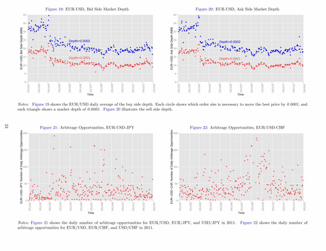
Figure 19: EUR-USD, Bid Side Market Depth
Depth=0.0001
Depth=0.0002
0
5
10
15
20
25
30
35
40
2011
/01
2011
/02
2011
/03
2011
/04
2011
/05
2011
/06
2011
/07
2011
/08
2011
/09
2011
/10
2011
/11
2011
/12
2012
/01
Time
EU
R−
US
D, B
id S
ide
Dep
th (
MM
)
Figure 20: EUR-USD, Ask Side Market Depth
Depth=0.0001
Depth=0.0002
0
5
10
15
20
25
30
35
40
2011
/01
2011
/02
2011
/03
2011
/04
2011
/05
2011
/06
2011
/07
2011
/08
2011
/09
2011
/10
2011
/11
2011
/12
2012
/01
Time
EU
R−
US
D, A
sk S
ide
Dep
th (
MM
)
Notes: Figure 19 shows the EUR/USD daily average of the buy side depth. Each circle shows which order size is necessary to move the best price by 0.0001, andeach triangle shows a market depth of 0.0002. Figure 20 illustrate the sell side depth.
Figure 21: Arbitrage Opportunities, EUR-USD-JPY
0
50
100
150
200
2011
/01
2011
/02
2011
/03
2011
/04
2011
/05
2011
/06
2011
/07
2011
/08
2011
/09
2011
/10
2011
/11
2011
/12
2012
/01
Time
EU
R−
US
D−
JPY,
Num
ber
of D
aily
Arb
itrag
e O
ppor
tuni
ties
Figure 22: Arbitrage Opportunities, EUR-USD-CHF
0
50
100
150
200
2011
/01
2011
/02
2011
/03
2011
/04
2011
/05
2011
/06
2011
/07
2011
/08
2011
/09
2011
/10
2011
/11
2011
/12
2012
/01
Time
EU
R−
US
D−
CH
F, N
umbe
r of
Dai
ly A
rbitr
age
Opp
ortu
nitie
s
Notes: Figure 21 shows the daily number of arbitrage opportunities for EUR/USD, EUR/JPY, and USD/JPY in 2011. Figure 22 shows the daily number ofarbitrage opportunities for EUR/USD, EUR/CHF, and USD/CHF in 2011.
24
7. Conclusions
EBS is the main interdealer market for the currency pairs EUR/USD, USD/JPY, EUR/JPY,
USD/CHF, and EUR/CHF. EBS decided to change the tick size, i.e., the minimum price improve-
ment, from pip pricing (four decimal points) to decimal pip pricing (five decimal points) for quoted
prices in March 2011. This decision has changed the EBS market’s microstructure significantly.
Our analysis shows that the EBS market’s structure enabled the high frequency traders to front-run
manual traders by the sub-penny jumping strategy. Manual traders typically place large orders in
the order book at prices ending in “0”, and they usually do not cancel their orders. Using this
information, HTFs place orders in front of manual traders by improving prices by the amount of
the minimum tick size. Once the sub-penny jumper trades, the orders he front-runs protect him
from serious losses on his position. If the price moves in his favor, the sub-penny jumper profits to
the full extent of the price changes. Therefore, the returns are unbounded for HFTs on one side
and limited on the other side.
We also show that the lower tick size helped HFTs be more aggressive in sub-penny jumping.
There is evidence from the data that supports our analysis of sub-penny jumping in the EBS
market. The distribution of the deal prices’ last digit is increasing for buyer-initiated deals and
is decreasing for seller-initiated deals. Using difference-in-difference regression, we find that the
spread as a liquidity cost decreased after the introduction of decimal pip pricing. However, due
to the implementation of the sub-penny jumping strategy by HFTs, manual traders were pushed
back in the order book and might face larger spreads. The market depth decreased after the tick
size change on both the bid and ask sides. HFTs use sub-penny jumping with smaller orders,
and manual traders have not used decimal pip pricing. These factors have led to shallower market
depth. Furthermore, there was no distinctive impact of the tick size change on the market efficiency
through triangular arbitrage opportunities.
25
Appendix A. Appendix
Suppose that the rate of return that the sub-penny jumper faces has a standard normal distribution:
x ∼ N(µ, σ2). In what follows, f, F will denote the pdf and cdf, respectively. Similarly, φ, Φ will
denote the pdf and cdf of the standard normal distribution.
f(x) =1√
2πσ2e−
12σ2
(x−µ)2 , φ(z) =1√2πe−
12z2
φ′(z) = −zφ(z) and φ(−z) = φ(z). The associated cumulative distribution function is
Φ(z) = Pr(Z ≤ z) =
∫ z
−∞φ(t)dt
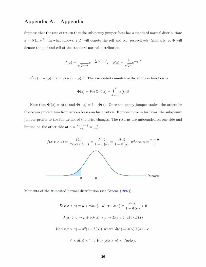
Note that Φ′(z) = φ(z) and Φ(−z) = 1 − Φ(z). Once the penny jumper trades, the orders he
front-runs protect him from serious losses on his position. If prices move in his favor, the sub-penny
jumper profits to the full extent of the price changes. The returns are unbounded on one side and
limited on the other side at a = p−(p+τ)p+τ = −τ
p+τ .
f(x|x > a) =f(x)
Prob(x > a)=
f(x)
1− F (a)=
φ(α)
1− Φ(α)where α =
a− µσ
µa Return
Moments of the truncated normal distribution (see Greene (1997)):
E(x|x > a) = µ+ σλ(α), where λ(α) =φ(α)
1− Φ(α)> 0
λ(α) > 0→ µ+ σλ(α) > µ→ E(x|x > a) > E(x)
V ar(x|x > a) = σ2(1− δ(α)) where δ(α) = λ(α)[λ(α)− α]
0 < δ(α) < 1→ V ar(x|x > a) < V ar(x).
26
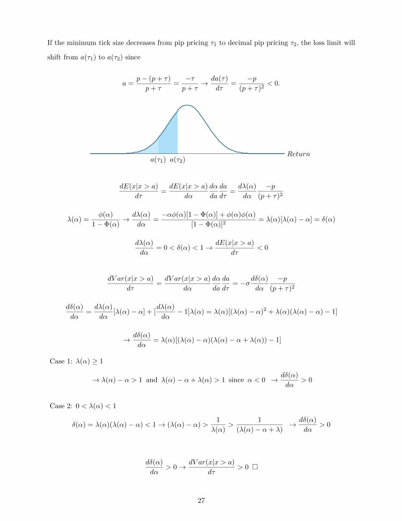
If the minimum tick size decreases from pip pricing τ1 to decimal pip pricing τ2, the loss limit will
shift from a(τ1) to a(τ2) since
a =p− (p+ τ)
p+ τ=−τp+ τ
→ da(τ)
dτ=
−p(p+ τ)2
< 0.
a(τ2)a(τ1)Return
dE(x|x > a)
dτ=dE(x|x > a)
dα
dα
da
da
dτ=dλ(α)
dα
−p(p+ τ)2
λ(α) =φ(α)
1− Φ(α)→ dλ(α)
dα=−αφ(α)[1− Φ(α)] + φ(α)φ(α)
[1− Φ(α)]2= λ(α)[λ(α)− α] = δ(α)
dλ(α)
dα= 0 < δ(α) < 1→ dE(x|x > a)
dτ< 0
dV ar(x|x > a)
dτ=dV ar(x|x > a)
dα
dα
da
da
dτ= −σdδ(α)
dα
−p(p+ τ)2
dδ(α)
dα=dλ(α)
dα[λ(α)− α] + [
dλ(α)
dα− 1]λ(α) = λ(α)[(λ(α)− α)2 + λ(α)(λ(α)− α)− 1]
→ dδ(α)
dα= λ(α)[(λ(α)− α)(λ(α)− α+ λ(α))− 1]
Case 1: λ(α) ≥ 1
→ λ(α)− α > 1 and λ(α)− α+ λ(α) > 1 since α < 0 → dδ(α)
dα> 0
Case 2: 0 < λ(α) < 1
δ(α) = λ(α)(λ(α)− α) < 1→ (λ(α)− α) >1
λ(α)>
1
(λ(α)− α+ λ)→ dδ(α)
dα> 0
dδ(α)
dα> 0→ dV ar(x|x > a)
dτ> 0 �
27
References
Ahn, H.-J., J. Cai, K. Chan, and Y. Hamao (2007). Tick size change and liquidity provision on the
Tokyo stock exchange. Journal of the Japanese and International Economics 21, 173–194.
Alexander, K. and T. Zabotina (2005). Is it time to reduce the minimum tick sizes of the E-Mini
futures? Journal of Futures Markets 25, 79–104.
Andersen, T., T. Bollerslev, D. Francis.X., and V. Clara (2003). Micro effects of macro announce-
ments: Real-time price discovery in foreign exchange. American Economic Review 93, 38–62.
Anshuman, V. R. and A. Kalay (1998). Market making with discrete prices. Review of Financial
Studies 11, 81–109.
Ascioglu, A., C. Comerton-Forde, and T. H. McInish (2010). An examination of minimum tick
sizes on the Tokyo stock exchange. Japan and the World Economy 22, 40–48.
Bacidore, J., R. Battalio, and R. Jennings (2001). Changes in order characteristics, displayed
liquidity and execution quality on the NYSE around the switch to decimal pricing. Working
paper, NYSE .
Bessembinder, H. (2000). Tick size, spreads, and liquidity: An analysis of NASDAQ securities
trading near ten dollars. Journal of Financial Intermediation 9, 213–239.
Bessembinder, H. (2003). Trade execution costs and market quality after decimalization. The
Journal of Financial and Quantitative Analysis 38, 747–777.
Bourghelle, D. and F. Declerck (2004). Why markets should not necessarily reduce the tick size.
Journal of Banking and Finance 28, 373–398.
Cai, J., Y. Hamaob, and R. Y. Ho (2008). Tick size change and liquidity provision for Japanese
stock trading near ¥1000. Japan and the World Economy 20, 19–39.
Chaboud, A. P., S. V. Chernenko, E. Howorka, R. S. Krishnasami Iyer, D. Liu, and J. H. Wright
(2004). The high-frequency effects of U.S. macroeconomic data releases on prices and trading
activity in the global interdealer foreign exchange market. Board of Governors of the Federal
Reserve System, International Finance Discussion Papers Number 823.
28
Chung, K. H. and C. Chuwonganant (2002). Tick size and quote revisions on the NYSE. Journal
of Financial Markets 5, 391–410.
Chung, K. H., K. A. Kim, and P. Kitsabunnarat (2005). Liquidity and quote clustering in a market
with multiple tick sizes. Journal of Financial Research 28, 177–195.
Cordella, T. and T. Foucault (1999). Minimum price variations, time priority and quote dynamics.
Journal of Financial Intermediation 8, 141–173.
Goldstein, M. A. and K. A. Kavajecz (2000). Eighths, sixteenths, and market depth: Changes in
tick size and liquidity provision on the NYSE. Journal of Financial Economics 56, 125–149.
Greene, W. H. (1997). Econometric Analysis, New York: Macmillan, 3rd edition.
Harris, L. E. (1994). Minimum price variations, discrete bid-ask spreads, and quotation sizes. The
Review of Financial Studies 7, 149–178.
Jones, C. M. and M. L. Lipson (2001). Sixteenths: Direct evidence on institutional execution costs.
Journal of Financial Economics 59, 253–278.
Kadan, O. (2006). So who gains from a small tick size? Journal of Financial Intermediation 15,
32–66.
Lallouache, M. and A. Frederic (2014). Tick size reduction and price clustering in a FX order book.
SSRN: http://ssrn.com/abstract=2297292 .
Schmidt, A. B. (2012). Ecology of the modern institutional spot FX: The EBS market in 2011.
SSRN: http://ssrn.com/abstract=1984070 .
29