n

Tiller, Ben (2016) Surface acoustic wave streaming in a PDMS microfluidic system: effect of frequency and fluid geometry & A remote ultrasonic glucose sensor. PhD thesis. http://theses.gla.ac.uk/7670/

Copyright and moral rights for this thesis are retained by the author A copy can be downloaded for personal non-commercial research or study, without prior permission or charge

This thesis cannot be reproduced or quoted extensively from without first obtaining permission in writing from the Author

The content must not be changed in any way or sold commercially in any format or medium without the formal permission of the Author

When referring to this work, full bibliographic details including the author, title, awarding institution and date of the thesis must be given

Glasgow Theses Service http://theses.gla.ac.uk/

theses@gla.ac.uk

Surface Acoustic Wave Streaming in a PDMS Microfluidic System: Effect of

Frequency and Fluid Geometry

&

A Remote Ultrasonic Glucose Sensor

Ben Tiller

A thesis submitted in the fulfilment of the requirements for the Degree of Doctor of Philosophy

School of Engineering

College of Science and Engineering

University of Glasgow

February 2016

ii

Abstract

This thesis describes two separate projects. The first is a theoretical and

experimental investigation of surface acoustic wave streaming in microfluidics.

The second is the development of a novel acoustic glucose sensor. A separate

abstract is given for each here.

Optimization of acoustic streaming in microfluidic channels by SAWs

Surface Acoustic Waves, (SAWs) actuated on flat piezoelectric substrates

constitute a convenient and versatile tool for microfluidic manipulation due to

the easy and versatile interfacing with microfluidic droplets and channels. The

acoustic streaming effect can be exploited to drive fast streaming and pumping

of fluids in microchannels and droplets (Shilton et al. 2014; Schmid et al. 2011),

as well as size dependant sorting of particles in centrifugal flows and vortices

(Franke et al. 2009; Rogers et al. 2010). Although the theory describing acoustic

streaming by SAWs is well understood, very little attention has been paid to the

optimisation of SAW streaming by the correct selection of frequency. In this

thesis a finite element simulation of the fluid streaming in a microfluidic

chamber due to a SAW beam was constructed and verified against micro-PIV

measurements of the fluid flow in a fabricated device. It was found that there is

an optimum frequency that generates the fastest streaming dependent on the

height and width of the chamber. It is hoped this will serve as a design tool for

those who want to optimally match SAW frequency with a particular microfluidic

design.

An acoustic glucose sensor

Diabetes mellitus is a disease characterised by an inability to properly regulate

blood glucose levels. In order to keep glucose levels under control some

diabetics require regular injections of insulin. Continuous monitoring of glucose

has been demonstrated to improve the management of diabetes (Zick et al.

2007; Heinemann & DeVries 2014), however there is a low patient uptake of

continuous glucose monitoring systems due to the invasive nature of the current

technology (Ramchandani et al. 2011). In this thesis a novel way of monitoring

glucose levels is proposed which would use ultrasonic waves to ‘read’ a

iii subcutaneous glucose sensitive-implant, which is only minimally invasive. The

implant is an acoustic analogy of a Bragg stack with a ‘defect’ layer that acts as

the sensing layer. A numerical study was performed on how the physical

changes in the sensing layer can be deduced by monitoring the reflection

amplitude spectrum of ultrasonic waves reflected from the implant. Coupled

modes between the skin and the sensing layer were found to be a potential

source of error and drift in the measurement. It was found that by increasing the

number of layers in the stack that this could be minimized. A laboratory proof of

concept system was developed using a glucose sensitive hydrogel as the sensing

layer. It was possible to monitor the changing thickness and speed of sound of

the hydrogel due to physiological relevant changes in glucose concentration.

iv

Table of Contents

Abstract ...................................................................................... ii

Acknowledgement ......................................................................... vii

Author’s Declaration ..................................................................... viii

Chapter 1 Introduction and motivations .............................................. 1

1.1 Development of an acoustic based glucose sensor .......................... 1

Diabetes mellitus ...................................................................... 1

The need to improve current glucose sensing technology ...................... 4

Continuous glucose monitoring; current on the mark technology ............. 5

Glucose measurement in the interstitial fluid .................................... 6

The foreign body response ........................................................... 6

Problems with current CGM technology ........................................... 7

Alternative sensors that made it to market ....................................... 8

Alternative methods of continuous glucose monitoring that did not make it to market ............................................................................... 8

A novel concept for glucose sensing based on ultrasonic waves. ............. 13

1.2 Surface acoustic wave streaming in microfluidics: effect of frequency and fluid length scale .................................................................. 15

Introduction to microfluidics ....................................................... 15

Introduction to SAW microfluidics ................................................. 16

Outline and motivation of the acoustic streaming study described in this thesis. .................................................................................. 19

Chapter 2 Background theory ......................................................... 23

2.1 Fundamentals of acoustics in different materials .......................... 23

Acoustics in solids .................................................................... 23

Rayleigh waves ....................................................................... 28

Leaky surface waves ................................................................. 31

Lamb waves ........................................................................... 32

2.2 Transmission and reflection of acoustic waves in layered media ........ 33

A single boundary .................................................................... 33

Reflections at many boundaries ................................................... 35

2.3 Piezoelectricity and ultrasonic transducers ................................. 38

Piezoelectricity ....................................................................... 39

Inter-digitated transducers for SAW generation ................................. 40

Thickness mode transducers ........................................................ 41

KLM equivalent circuit for transducer modelling ................................ 42

v

2.4 Acoustic streaming .............................................................. 45

Acoustic streaming background .................................................... 45

An example of acoustic streaming by a plane wave. ........................... 46

Chapter 3 Materials and methods ..................................................... 48

3.1 SAW experiments. ............................................................... 48

Fabrication and design of IDTs. .................................................... 48

Fabrication of PDMS microchambers .............................................. 51

Experimental set-up and channel network design. ............................. 52

Laser Doppler vibrometer measurements ........................................ 54

PIV measurements ................................................................... 54

3.2 Ultrasonic glucose sensor experiments ....................................... 57

Details of ultrasonic transducer used in experiments .......................... 58

Details of experiments with acoustic layered systems ......................... 59

Fabrication of hydrogel ............................................................. 60

Optical measurements of hydrogel thickness .................................... 61

3.3 Details of COMSOL simulations ................................................ 62

Streaming from Leaky SAWs – sound field in fluid domain ..................... 63

Streaming from Leaky SAWs – fluid flow simulation ............................ 65

Acoustic waves in elastic and fluid materials .................................... 65

Chapter 4 Development of SAW streaming simulation ............................. 68

4.1 Development of the sound field and body force equations. .............. 69

4.2 Vibrometer measurements ..................................................... 77

Amplitude of SAW beam in PDMS chamber ....................................... 78

Amplitude of SAW beam in the tunnel ............................................ 81

Chapter 5 SAW streaming in a PDMS chamber, effect of frequency. ............ 84

5.1 Micro PIV measurements of fluid streaming compared with simulation results. ................................................................................... 84

5.1.1 Comparison of streaming magnitudes ................................... 92

5.2 Impact of measurement error ................................................. 94

5.3 Conclusions ....................................................................... 97

5.4 Effect of frequency on streaming magnitudes for different chamber geometries ............................................................................... 97

Power loss due to PDMS wall ...................................................... 101

5.5 Conclusions and outlook ....................................................... 102

Limitations of the simulation ...................................................... 102

Conclusions........................................................................... 104

Chapter 6 A first step towards an ultrasonic glucose sensor. .................... 105

6.1 Introduction and overview .................................................... 105

6.2 Acoustic reflections from a layered system ‘1D case’. ................... 108

vi

6.2.1 The simplest case .......................................................... 108

KLM model and skin layer .......................................................... 114

Porosity ............................................................................... 120

6.3 Incidence angle ................................................................. 123

6.4 Conclusions ...................................................................... 128

Chapter 7 A second step towards an ultrasonic glucose sensor ................. 130

7.1 Introduction and Overview .................................................... 130

Boronic acid as a glucose sensor .................................................. 130

Glucose sensing with boronic acid incorporated hydrogels ................... 131

Glucose sensing polymer solutions using boronic acid ......................... 132

Alternative glucose sensing molecules ........................................... 133

Ultrasonic characterisation of hydrogels ........................................ 133

7.2 Model verification experiments .............................................. 134

Single liquid layer system .......................................................... 134

Multiple layers structure. .......................................................... 140

7.3 Glucose sensitive hydrogel experiments .................................... 144

Fabrication and experimental method ........................................... 144

Group delay and thickness measurements ...................................... 145

Group delay measurements........................................................ 147

Sound velocity fitting ............................................................... 148

Effect of glucose addition on resonance position .............................. 148

Response of hydrogel over time .................................................. 150

7.4 Conclusion ....................................................................... 152

Chapter 8 Wider perspectives and future work .................................... 155

8.1 Further steps towards an in vivo acoustic glucose sensor ................ 155

8.2 Acoustic Bragg-stacks as sensors in general ................................ 156

8.3 PDMS tunnel concept ........................................................... 158

8.4 SAW streaming in microfluidic channels .................................... 158

Alternatives to PDMS ............................................................... 158

SAW induced boundary streaming ................................................ 158

List of References ........................................................................ 160

vii

Acknowledgement

Firstly I would like to thank my supervisor, professor Jon Cooper for his wise

guidance without whom this work would not have been possible. I would also like

to thank various members of the biomedical research team who have

contributed their knowledge and advice, to Julian Rebound and Rab Wilson, the

SAWsome, SAW, SAWsperts, who shaped and influenced my thinking in

immeasurably. Also to Andrew Glidle for sitting each one of my internal vivas

and keeping me on the straight and narrow. Thanks also to everyone who work

on level 8, it has made for a lovely working environment to be among such great

people.

On a more personal level I would also like to thank Mahuta Bala for many games

of chess, Emrah Kaplan for informative conversations and Niall Geoghegan for

great banter. The biomedical football group should also get a special mention,

although one is sometimes confused as to what is on show – sport or comedy it

has all helped to alleviate stress and for this I am thankful.

Lastly my sincerest thanks and love go to my family, without whose constant

support and love I would not even have graduated with a degree, let alone finish

a thesis. My love and thanks to all of you. To my Grandparents especially, who

have literally kept me afloat financially, I feel as if you have part-funded this

thesis.

Very very lastly I would like to thank my girlfriend Elske Thaden, whose support

and love has kept me afloat emotionally. I love you.

viii

Author’s Declaration

I declare that, except where explicit reference is made to the contribution of

others, that this dissertation is the result of my own work and has not been

submitted for any other degree at the University of Glasgow or any other

institution.

Chapter 4 page 1

Chapter 1 Introduction and motivations

Two different applications of using Ultrasonics to interact with materials at the

micro-scale are investigated in this thesis. A numerical and experimental study

on acoustic streaming in microfluidic channels by Rayleigh surface acoustic

waves (SAWs), and a novel acoustic glucose sensor. These are both individual

projects in their own right, however they are also connected in that they are

both examples of the exploitation of acoustic waves at the sub-millimetre length

scale, and therefore have potential overlap in future small scale applications.

This introduction starts in section 1.1 with a background to diabetes and its

management, and then goes on to examine the current state of glucose sensing

technology and the areas where improvement is needed. The subject of this

thesis, a remote acoustic glucose sensor concept, is then introduced as a

potential solution for some of these problems.

In section 1.2 the other half of this thesis is introduced, SAW induced streaming

in a microfluidic chamber. This starts with a brief introduction to microfluidics

and then explains why fluid actuation by SAWs plays an important role in various

microfluidics applications. The subject of this thesis on SAW streaming in PDMS

microfluidics is then placed into context with this work.

1.1 Development of an acoustic based glucose sensor

This section starts with an introduction to the disease Diabetes mellitus, the

severity of the disease, the need for better monitoring of glucose levels and the

enormous effort that has gone into development of a continuous blood glucose

monitoring system.

Diabetes mellitus

As of 2011 an estimated 340 million people worldwide suffer from diabetes

mellitus, (Danaei et al. 2011) a disease where the body has an impaired or total

inability to properly regulate glucose concentrations in the blood. Prolonged

periods of high blood glucose levels are associated with a wide range of macro

and micro vascular diseases such as nephropathy, stroke, coronary artery disease

Chapter 1 page 2 and retinopathy, (Shaw & Cummings 2012) through these associated

complications, diabetes is estimated to kill 3.96 million people per year (Roglic

& Unwin 2010). Diabetic retinopathy affects 87-98% of diabetics after 30 years of

having the disease and 2% of all diabetics are blind (Shaw & Cummings 2012).

Treatment of Diabetes cost the UK Nation Health Service approximately £23.7

billion in direct costs in the year 2010/2011, 10% of total health resource

expenditure. This has been projected to increases to £39.8 billion by the year

2035/2036 due to the increasing prevalence of the disease (Hex et al. 2012).

There is currently no cure for diabetes and instead it is managed by using various

different strategies to control blood-glucose levels, ranging from diet control to

regular injections of insulin. There is a strong consensus that better

management of the disease can be achieved through improved monitoring of

blood glucose levels which would then reduce the likelihood of a patient

developing the chronic diseases described above (Oliver et al. 2009).

In healthy subjects the body automatically regulates the concentration of

glucose in the blood using the hormones insulin and glucagon. Insulin triggers the

liver, adipose and muscle tissues to take up glucose and store it as glycogen

lowering blood glucose levels. Glucagon serves as the antagonist of insulin in

that it encourages break down of glycogen in the liver into glucose which is then

released in the blood stream. The alpha and beta cells of the pancreas which

secrete these hormones are responsible for controlling overall glucose

concentrations via the controlled release of these hormones (Norman & Litwack

1997). Normal blood glucose levels lie within the range 4.4-6.1 mmol L-1. After a

meal these will temporarily increase as extra glucose is introduced into the

bloodstream, in response the pancreas releases more insulin in order to bring the

glucose levels under control. In diabetic patients the body cannot control

glucose levels appropriately and without treatment much higher glucose

concentrations (hyperglycaemia) are typical.

Diabetes is classified into two main types. Patients with type 1 cannot make

insulin because the beta cells that produce it are progressively destroyed by an

autoimmune disorder (Watkins 2004). Type 1 diabetes affects 10-15% of all

diabetics and is the most severe form of diabetes (Ekoe et al. 2008). These

patients need regular bolus injections of insulin to survive. These injections are

Chapter 1 page 3 timed to mimic natural insulin release in the body and can involve the use of

several different types of insulin which have a different rate of action on glucose

concentration. Intermediate and long acting insulin analogs are used to mimic

the background levels of insulin in the body while short acting insulin is used at

meal times to mimic the prandial release of insulin immediately after a meal

(Zazworksky et al. 2006).

85-90% of diabetics have type 2 diabetes (Ekoe et al. 2008). In patients with type

2 diabetes there is either an impaired ability to secrete insulin or a resistance to

its action and is due to a combination of genetic and environmental factors such

as over consumption of food (Watkins 2004). In the last half century there has

been a huge increase in the numbers of people with type 2 diabetes worldwide,

due in large to part the dramatic increases in obesity. The total number of

people with diabetes in Europe has roughly doubled since 1970 (Ekoe et al.

2008). Management of type 2 diabetes depends on severity, as the disease tends

to get worse over time. Initially glucose levels can be managed through an

appropriate diet and exercise regime, however over time oral medications

designed to lower blood glucose levels such as metaformin and secretagogues as

well as direct insulin injections become necessary to maintain glycaemic control

(Nathan et al. 2009).

For type 1 and some type 2 diabetics regular insulin injections are necessary,

however determination of the amount of insulin to inject can be difficult to

manage. A post meal injection of insulin requires a measurement of pre-meal

glucose levels along with a calculation of the total carbohydrate and sugar

content of the meal. A danger is over estimation of the insulin dose which can

lead to a crash in glucose levels and midday hypoglycaemia. Nocturnal

hypoglycaemia can also be a recurring problem for some diabetics where sleep

prevents awareness of the crash in glucose levels (Zazworksky et al. 2006). This

can be extremely serious because hypoglycaemia can ultimately lead to coma

and death since the brain relies on glucose as its only fuel source. Intensive

insulin therapy can reduce the development of long term complications however

this requires greater involvement from the patient to properly monitor blood

glucose levels and administer insulin, which can lead to an increased risk of

Chapter 1 page 4 hypoglycaemia (The diabetes control and complication trial research group 1993)

(Uk prospective diabetes study group 1998).

The need to improve current glucose sensing technology

Crucial to the improved management of diabetes is therefore the accurate and

regular monitoring of blood glucose levels so as to inform appropriate insulin

doses and warn against the onset of hypoglycaemia. There has been a gigantic

effort by various different research groups over the last 30 years to improve the

current state of glucose sensing technology. In spite of this the dominant method

of patient self-monitoring is still based on extracting a drop of blood from the

finger in order to measure glucose levels (Aggidis et al. 2015). On the one hand

this is a highly evolved technology and provides a very accurate, reliable and

specific measurement of glucose concentration. A droplet of blood is extracted,

usually from the finger-tip and applied to a disposable test-strip which is then

‘read’ by a device which displays the glucose concentration. However on the

other hand extraction of the blood droplet is painful to the patient, and each

individual measurement requires the use of a fresh test strip which limits to the

sensible number of measurements than can be made throughout the day. A

significant issue with this is missing periods of hypoglycaemia that occur

between measurements and in the absence of monitoring capability such as at

night or while the patient is driving (Aggidis et al. 2015).

There are currently 5 companies that dominate the market for finger prick style

glucose meters, Roche 24%, Lifescan 20%, Bayer 13%, Abbot 11% and Beijing

Yicheng 32% (Aggidis et al. 2015). These companies produce a range of different

devices that work on very similar fundamental principles using an

electrochemical method to detect glucose via redox reactions initiated with an

immobilised enzyme such as glucose oxidase or glucose dehydrogenase (Aggidis

et al. 2015).

A method that is able to continuously monitor glucose levels should therefore

have a significant advantage for patients in the management of their disease.

This has been backed up by numerous studies that suggest continuous glucose

monitoring in type 1 diabetics improves glycaemic control due to easier

identification of post prandial and sleeping hypoglycaemia, as well as in patients

Chapter 1 page 5 who cannot feel the onset of hypoglycaemia (Diabetes Research in Children

Network Study Group et al. 2009; Denis et al. 2009; Pickup et al. 2011;

Heinemann & DeVries 2014) In type 2 diabetics who require daily insulin

injections continuous glucose monitoring has also been observed to improve

glycaemic control and reduce incidences of hypoglycaemia, especially at night

(Zick et al. 2007). There is also a study that suggests an improvement in

glycaemic control for type 2 diabetics who are not on daily insulin injections due

to the improvement in the quality of the information that continuous glucose

monitoring provides over time point measurements i.e. trends in glucose levels

due to exercise, meals and insulin injections. This group forms the majority of

those with type 2 diabetes (Vigersky et al. 2012).

Another possibility continuous glucose monitoring opens up is the realisation of a

closed loop insulin delivery system, or ‘artificial pancreas’. Where a continuous

glucose monitoring system is linked to an insulin pump and informs automatic

injections insulin (Lodwig et al. 2014).

Continuous glucose monitoring; current on the mark technology

Continuous glucose monitoring (CGM) devices have been commercially available

for patient self-monitoring since 1999 when Mini-Med released a system based on

an electrochemical assay exploiting the redox reaction between glucose and

glucose oxidase (Mastrototaro 2000). This worked by percutaneous implantation

of an electrode under the skin in the form a needle. The sensing needle had a

relatively short life-span and needed replacement every three days. Daily

calibration steps using finger stick measurements as a comparison were also

required due to significant sensor drift caused by foreign body resistance to the

implant and enzyme instability (Oliver et al. 2009).

At the time of writing, all the available continuous glucose monitoring systems

on the UK market follow this fundamental principle of glucose sensing, i.e. using

an enzymatic electrode inserted into the skin. In the UK this amounts to seven

continuous glucose monitoring systems available for purchase from three

different companies, Abbott, Dexcom and Medtronics. Improvements in this

technology since 1999 have so far been largely incremental and have involved

improving selectivity by restricting access to the electrode from electroactive

Chapter 1 page 6 compounds which can cause false signals. Another problem with these sensors is

known as the oxygen deficit, which is the fact that oxygen is present in much

lower quantities than glucose in the interstitial fluid: oxygen is required in the

reaction catalysed by glucose oxidase that converts glucose to gluconic acid and

hydrogen peroxide. These problems have been addressed by introduction of

membranes which limit the transport of glucose to the electrode, readjusting

the ratio between glucose and oxygen at the electrode (Gifford 2013). However

for most of the sensors on the market the fundamental difficulties still largely

remain, i.e. the need for frequent calibration, a short sensor lifetime (slightly

increased to approx. 12-14 days) and the pain and irritation caused by a

percutaneous implant (Freckmann et al. 2015). The exception is the FreeStyle

Libre (Abbott Diabetes Care, Almeda CA) which was introduced in 2014 and has

the significant advantage that in that it only requires factory calibration,

thereby eliminating the hassle of daily finger stick calibrations throughout its 14

day lifetime (Wang & Lee 2015). Recent clinical trials have shown good stability

and accuracy over this time period (Bailey et al. 2015).

Glucose measurement in the interstitial fluid

The percutaneous electrochemical sensors described above do not measure

blood glucose levels directly but rather glucose levels in the interstitial fluid.

The interstitial fluid bathes the tissue cells of the body and acts as the medium

between the blood supply and tissue cells. A healthy human adult contains

around 12-15 litres of interstitial fluid (Ebah 2012). Nutrients such as glucose can

permeate from blood capillaries into the interstitial fluid and glucose

concentrations in the interstitial fluid are therefore correlated with blood

glucose levels, however glucose changes in the interstitial fluid tend to lag

behind changes in the blood. This lag time varies with the physical state of the

patient and the rate of concentration changes, however under normal conditions

when glucose levels are not rapidly changing(e.g. due to exercise) the lag time

ranges between 5 and 10 minutes (Nichols et al. 2013).

The foreign body response

The foreign body response is an important factor for any glucose sensing

implanted device since the inflammation, encapsulation and attempts at

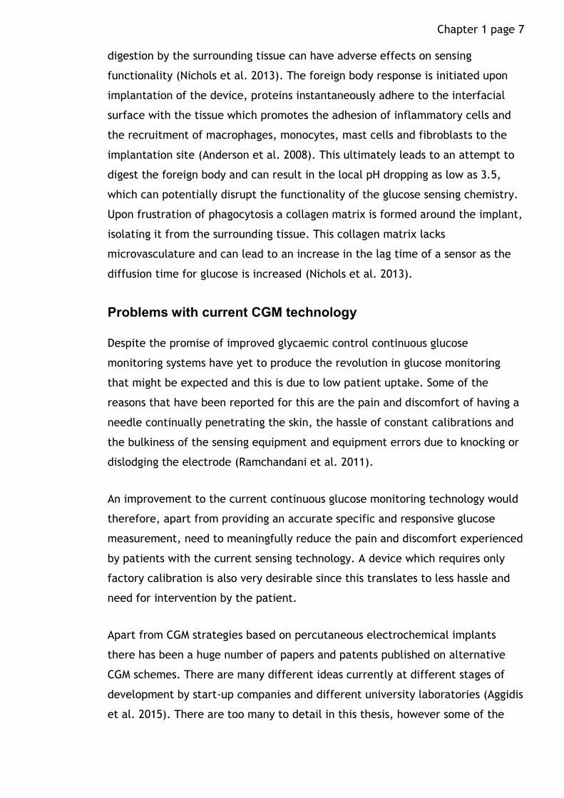
Chapter 1 page 7 digestion by the surrounding tissue can have adverse effects on sensing

functionality (Nichols et al. 2013). The foreign body response is initiated upon

implantation of the device, proteins instantaneously adhere to the interfacial

surface with the tissue which promotes the adhesion of inflammatory cells and

the recruitment of macrophages, monocytes, mast cells and fibroblasts to the

implantation site (Anderson et al. 2008). This ultimately leads to an attempt to

digest the foreign body and can result in the local pH dropping as low as 3.5,

which can potentially disrupt the functionality of the glucose sensing chemistry.

Upon frustration of phagocytosis a collagen matrix is formed around the implant,

isolating it from the surrounding tissue. This collagen matrix lacks

microvasculature and can lead to an increase in the lag time of a sensor as the

diffusion time for glucose is increased (Nichols et al. 2013).

Problems with current CGM technology

Despite the promise of improved glycaemic control continuous glucose

monitoring systems have yet to produce the revolution in glucose monitoring

that might be expected and this is due to low patient uptake. Some of the

reasons that have been reported for this are the pain and discomfort of having a

needle continually penetrating the skin, the hassle of constant calibrations and

the bulkiness of the sensing equipment and equipment errors due to knocking or

dislodging the electrode (Ramchandani et al. 2011).

An improvement to the current continuous glucose monitoring technology would

therefore, apart from providing an accurate specific and responsive glucose

measurement, need to meaningfully reduce the pain and discomfort experienced

by patients with the current sensing technology. A device which requires only

factory calibration is also very desirable since this translates to less hassle and

need for intervention by the patient.

Apart from CGM strategies based on percutaneous electrochemical implants

there has been a huge number of papers and patents published on alternative

CGM schemes. There are many different ideas currently at different stages of

development by start-up companies and different university laboratories (Aggidis

et al. 2015). There are too many to detail in this thesis, however some of the

Chapter 1 page 8 most prominent areas of current development and interesting failed attempts

are now discussed.

Alternative sensors that made it to market

The GlucoWhatch (Cygnus Inc., Red-Wood City, CA, USA) was available for a

short time-between 2001 and 2008. This used a trans-dermal method called

reverse iontophoresis to extract interstitial fluid from the skin noninvasively i.e.

without breaking the skin. The fluid could then be interrogated via the usual

electrochemical method. Unfortunately there were severe technical drawbacks,

the most important being the absence of functionality when sweat was present

on the skin and reported skin irritation (Oliver et al. 2009).

Another device that made it to market was the PENDRA (Pendragon medical Ltd,

Zurich Switzerland) which was released in European markets in 2004. This

indirectly measured glucose concentration by impedance spectroscopy at the

skin. Changes in impedance are related to sodium and potassium gradients,

which are correlated to glucose concentration. However the device proved to be

very inaccurate and was withdrawn (Mcgarraugh 2009).

Alternative methods of continuous glucose monitoring that did not make it to market

There are a wide variety of different continuous glucose monitoring methods

that have been reported but as of yet have not made it to market or are still in

development. These roughly fall into a few subcategories dependant on the

underlying principle.

Non-invasive techniques

Non-invasive techniques aim to develop a continuous glucose sensor that does

not cause the patient as much and pain and irritation as electro-chemical

sensors where a needle continuously breaks the skin.

Optical spectroscopic methods

A wide variety of methods have been tried based on using light to sense glucose

concentration in the skin. Near-Infrared diffusion spectroscopy is a technique

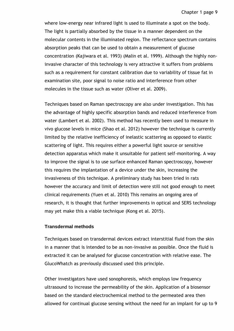
Chapter 1 page 9 where low-energy near infrared light is used to illuminate a spot on the body.

The light is partially absorbed by the tissue in a manner dependent on the

molecular contents in the illuminated region. The reflectance spectrum contains

absorption peaks that can be used to obtain a measurement of glucose

concentration (Kajiwara et al. 1993) (Malin et al. 1999). Although the highly non-

invasive character of this technology is very attractive it suffers from problems

such as a requirement for constant calibration due to variability of tissue fat in

examination site, poor signal to noise ratio and interference from other

molecules in the tissue such as water (Oliver et al. 2009).

Techniques based on Raman spectroscopy are also under investigation. This has

the advantage of highly specific absorption bands and reduced interference from

water (Lambert et al. 2002). This method has recently been used to measure in

vivo glucose levels in mice (Shao et al. 2012) however the technique is currently

limited by the relative inefficiency of inelastic scattering as opposed to elastic

scattering of light. This requires either a powerful light source or sensitive

detection apparatus which make it unsuitable for patient self-monitoring. A way

to improve the signal is to use surface enhanced Raman spectroscopy, however

this requires the implantation of a device under the skin, increasing the

invasiveness of this technique. A preliminary study has been tried in rats

however the accuracy and limit of detection were still not good enough to meet

clinical requirements (Yuen et al. 2010) This remains an ongoing area of

research, it is thought that further improvements in optical and SERS technology

may yet make this a viable technique (Kong et al. 2015).

Transdermal methods

Techniques based on transdermal devices extract interstitial fluid from the skin

in a manner that is intended to be as non-invasive as possible. Once the fluid is

extracted it can be analysed for glucose concentration with relative ease. The

GlucoWhatch as previously discussed used this principle.

Other investigators have used sonophoresis, which employs low frequency

ultrasound to increase the permeability of the skin. Application of a biosensor

based on the standard electrochemical method to the permeated area then

allowed for continual glucose sensing without the need for an implant for up to 9

Chapter 1 page 10 hours (Chuang et al. 2004). Like the GlucoWhatch this would presumably suffer

from similar problems due to interference from sweat.

Semi-invasive techniques, subcutaneous implants

A variety of strategies based on fully implanted devices that monitor glucose

levels in the interstitial fluid have also been suggested for glucose sensing. This

is argued as an improvement on the ‘wired’ electrochemical sensors because the

skin is not continuously broken once the device has been implanted. One of the

challenges with this strategy is the need for a wireless communication method

that can operate through the skin. Another issue is the foreign body response to

the implant which, as with the ‘wired’ sensors can increase lag time and affect

sensor stability.

Radio frequency transmission

Fully implanted electrochemical sensors containing transmitters to send glucose

measurements via radio waves have been tried (Gilligan et al. 2004). These

have been implanted into pigs and were able to monitor glucose for up to 520

days (Gough et al. 2010). However batteries are required to power the

transmitter and this greatly increases the footprint of the implant, which

increases the invasiveness and complexity of implantation.

Fluorescence techniques

Fluorescence techniques based on measuring the fluorescence intensity of a

subcutaneously implanted device sensitive to glucose have also been tried. This

raises problems of biocompatibility of the molecules and signal strength, since

the florescence needs to be detected through the skin which significantly

absorbs light in the visible wavelength(Nichols et al. 2013). Recently hydrogels

containing a fluorescent molecule sensitive to glucose have been investigated as

in-vivo glucose sensors in mice (Heo et al. 2011; Shibata et al. 2010). These were

able to track glucose over a period of 140 days by measuring the fluorescence

intensity. However miniaturization of the equipment required for exciting and

detecting the fluorescence intensity is not currently possible to a size

appropriate for a personalized device for continuous monitoring (Nichols et al.

2013).

Chapter 1 page 11

Infrared scattering

Skin is highly absorbing in the visible and higher frequency electromagnetic

spectrum however at infrared frequencies scattering and absorption by the skin

is greatly reduced. A potential strategy exploiting this has been described in,

(Vezouviou & Lowe 2015) where a sensing concept was developed measuring the

near-infrared reflection spectrum from a hydrogel patterned with gold

nanoparticles. The hydrogel changes volume with glucose concentrations and

therefore the spacing between the lines of gold nanoparticles changes, which

causes a shift in the peak diffraction wavelength.

Glucose sensitive Hydrogels

Many sensing strategies have been proposed using glucose sensitive hydrogels to

monitor glucose levels. There are many different ways glucose sensitive

hydrogels can be incorporated into an overall continuous glucose sensing

strategy, most proposals fall under the semi-invasive strategy where the

hydrogel is implanted in some form and reacts to changing glucose

concentrations in the interstitial fluid.

Hydrogels are hydrophilic chains of one or more monomers that have been cross-

linked together in a polymerisation reaction. Due to their hydrophilic properties

these networks can absorb large quantities of water in between the polymer

chains which results in a soft gel like substance that keeps its shape. The

crosslinks hold the network together, stop the water from flowing away and the

polymer chains from dissolving. Hydrogels can be as much as 90-95 % water and

have elastic properties similar to body tissue. For this reason hydrogels are of

great interest in bioengineering for their biocompatible and swelling properties

(Ulijn et al. 2007).

They can also form a scaffold on which to do biochemical sensing by

incorporating chemically sensitive molecules in the chain network of the

hydrogel. Analytes can diffuse through the porous hydrogel network and react

with the sensing molecules causing a physical change either in florescence or the

chemical potential of the hydrogel leading to swelling/contraction. Glucose

sensitive hydrogels have been realised by incorporating glucose sensing

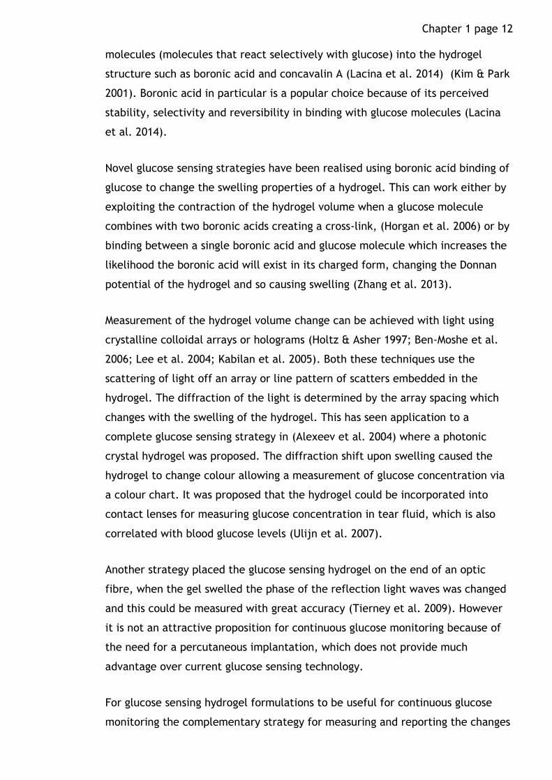
Chapter 1 page 12 molecules (molecules that react selectively with glucose) into the hydrogel

structure such as boronic acid and concavalin A (Lacina et al. 2014) (Kim & Park

2001). Boronic acid in particular is a popular choice because of its perceived

stability, selectivity and reversibility in binding with glucose molecules (Lacina

et al. 2014).

Novel glucose sensing strategies have been realised using boronic acid binding of

glucose to change the swelling properties of a hydrogel. This can work either by

exploiting the contraction of the hydrogel volume when a glucose molecule

combines with two boronic acids creating a cross-link, (Horgan et al. 2006) or by

binding between a single boronic acid and glucose molecule which increases the

likelihood the boronic acid will exist in its charged form, changing the Donnan

potential of the hydrogel and so causing swelling (Zhang et al. 2013).

Measurement of the hydrogel volume change can be achieved with light using

crystalline colloidal arrays or holograms (Holtz & Asher 1997; Ben-Moshe et al.

2006; Lee et al. 2004; Kabilan et al. 2005). Both these techniques use the

scattering of light off an array or line pattern of scatters embedded in the

hydrogel. The diffraction of the light is determined by the array spacing which

changes with the swelling of the hydrogel. This has seen application to a

complete glucose sensing strategy in (Alexeev et al. 2004) where a photonic

crystal hydrogel was proposed. The diffraction shift upon swelling caused the

hydrogel to change colour allowing a measurement of glucose concentration via

a colour chart. It was proposed that the hydrogel could be incorporated into

contact lenses for measuring glucose concentration in tear fluid, which is also

correlated with blood glucose levels (Ulijn et al. 2007).

Another strategy placed the glucose sensing hydrogel on the end of an optic

fibre, when the gel swelled the phase of the reflection light waves was changed

and this could be measured with great accuracy (Tierney et al. 2009). However

it is not an attractive proposition for continuous glucose monitoring because of

the need for a percutaneous implantation, which does not provide much

advantage over current glucose sensing technology.

For glucose sensing hydrogel formulations to be useful for continuous glucose

monitoring the complementary strategy for measuring and reporting the changes

Chapter 1 page 13 in the hydrogel is also important. Furthermore the hydrogel has to be placed so

that it is continuously exposed to the bodily changes in glucose levels. Strategies

based on the diffraction of light such as crystalline colloidal arrays and

holograms etc, would face problems of how to take the measurement through

the skin without recourse to a percutaneous implantation.

A novel concept for glucose sensing based on ultrasonic waves.

This thesis explores a novel concept for continuous glucose sensing that uses

ultrasonic waves to communicate wirelessly with a potentially implantable

glucose sensing device. In this scheme an ultrasonic transducer sends signals

across the skin to a device that has been subcutaneously implanted and

measures the reflections from the device. The implant is designed in such a way

that the ultrasonic reflection spectrum can be used to infer the interstitial

glucose concentration. This had been done using an acoustically analogous

version of a Fabry-Perot stack that consists of alternating plane parallel layers.

The reflection coefficient from such a stack can be engineered to have sharp

resonances due to constructive and destructive interference of ultrasonic

reflections between the layers within the stack. The frequency positon of these

resonances depend of the physical properties of the layers, i.e. the thickness

and speed of sound. By linking the physical properties of one of these layers with

glucose concentration an alternative strategy for continuous glucose monitoring

could be realised. Changes in the mechanical properties of a layer are linked to

glucose concentrations by incorporating a boronic acid based hydrogel as one of

the layers in the stack. The volumetric changes in the hydrogel are measured as

changes in the frequency positon of a resonance peak.

The advantages inherent in such a method would be the non-invasiveness of a

subcutaneous implant as opposed to a percutaneous one and no requirement for

an in-vivo power supply or on board circuitry such an induction coils etc.

Furthermore the use of boronic acid based hydrogels provides a stable selective

and potentially accurate method for sensing glucose concentrations, which might

have some advantage over enzyme based sensing methods which can suffer from

denaturation and degradation (Kotanen et al. 2012).

Chapter 1 page 14

Outline of the glucose sensing chapters in the thesis

In this thesis the results from a computational and experimental study on the

feasibility of the glucose sensing concept describe above is presented. The flow

of information is as follows. In chapter 2 (background theory), the equations

used to simulate acoustic reflections in layered media are described. The basic

theory of acoustic waves is also described. In chapter 3 (materials and methods),

the fabrication protocol for the hydrogel and layered structures used in the

experiments are described. The details of a COMSOL simulation used to model

the reflection from a layered structure at an angle is described. Chapter 6 then

presents the results of a series of simulations which investigates the principles

for how a layered stack should be fabricated. It is shown that measurement

errors can occur from changes in the physical properties of the skin tissue

between the transducer and the implant and also changes in the incidence angle

of the acoustic beam relative to the implant. A solution for these based on a

reference measurement and the proper design of the layered stack is suggested.

Chapter 7 investigates the measurement of a prototype acoustic layered stack

where one of the physical properties of the layers is systematically changed.

This is first investigated in a controlled way using different concentrations of

salt water as one of the layers. This experiment demonstrates the potential

accuracy of this measurement. A glucose sensitive polyacrylamide hydrogel is

then incorporated as one of the acoustic layers. This hydrogel contracts with

increasing glucose concentration and the contraction leads to a change in the

thickness and speed of sound in the hydrogel layer. It is shown that

physiologically relevant glucose concentrations can in principle be measured

using this technique.

Chapter 1 page 15

1.2 Surface acoustic wave streaming in microfluidics: effect of frequency and fluid length scale

This section introduces microfluidics as an important concept in bio-medical

engineering. The application of SAWs for actuating and pumping in microfluidics

is then introduced. Then the subject of this thesis, a numerical and

experimental study on SAW streaming in microfluidic chambers is introduced and

the motivation for doing the work is explained.

Introduction to microfluidics

Microfluidics is the study of the control and manipulation of fluids on the sub

mm length scale. This has largely been made possible by the adoption of MEMs

fabrication technologies developed in the semiconductor industry to create

devices that can be used to control and manipulate fluids (Sackmann et al.

2014). These usually take the form of networks of channels with length scales on

the order of 1-1000 µm that a fluid sample can be induced to move through. The

ability to manipulate tiny volumes of fluid leads to many exciting possibilities for

the medical and biological sciences. Chemical assays can be performed using

only tiny sample volumes, potentially reducing the cost of reagents. The

potential scalability is also greatly increased with the prospect of performing

multiple parallel assays from one sample on a small microfluidic device. One

example is the detection of HIV and Syphilis via an ELISA assay performed on a

portable and cheap microfluidic chip (Chin et al. 2011). Furthermore since

feature sizes can be fabricated on the length scale of cells, microfluidics has

also proven to be a useful tool for cell manipulation and control. For example

circulating tumour cells have been isolated from a whole blood sample using a

microfluidic device (Nagrath et al. 2007; Stott et al. 2010).

Initially microfluidic devices were manufactured from the same materials used in

the semi-conductor industry, silicon and glass. However these had significant

limitations like complex bonding protocols, inflexibility and in the case of silicon

opacity (Sackmann et al. 2014). In 1998 Whiteside pioneered the use of PDMS, a

flexible, elastic and importantly transparent polymer to create microfluidic

channels (Duffy et al. 1998). PDMS as a material has a number of advantages in

that it is relatively easy to pattern fluid channels into it, it is transparent which

Chapter 1 page 16 makes it compatible with various microscopy techniques, its surface chemistry

can be tuned to be either hydrophilic or hydrophobic and it can be bonded

(reversibly or irreversibly) to glass coverslips and other substrates including

itself. Due to these advantages PDMS has become a very popular material in

many microfluidics applications (Sackmann et al. 2014).

Introduction to SAW microfluidics

Recently there has been a growing interest in using surface acoustic waves (SAW)

to perform different processing steps in microfluidic systems. SAW devices

provide an attractive platform for integration with microfluidics because of their

small size, easy incorporation within a PDMS microchannel system and easy

digital integration. There is a rich array of different physical effects that can be

elicited with SAW technology which makes it a potentially multipurpose tool for

fluid and cell handling.

SAWs are actuated on flat piezoelectric substrates where an alternating electric

field is applied to a shaped metal electrode called an IDT. The electric field at

the IDT creates deformations in the substrate along the fingers of the IDT which

constructively interfere with each other to produce surface waves that

propagate away from the IDT. A fluid placed in the path of these surface waves

will absorb some of the energy of the SAWs as they pass along the interface

between the SAW substrate and the fluid. The absorbed energy takes the form of

a longitudinal pressure wave that propagates into the fluid at the Rayleigh

angle. These pressure waves can cause fast streaming and this fact can be

exploited in droplets and fluids in microfluidic channels placed in the path of the

SAW beam.

Chapter 1 page 17

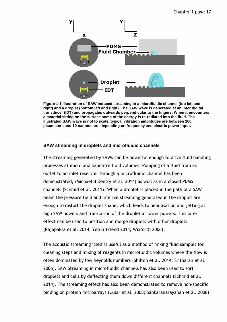
Figure 1-1 Illustration of SAW induced streaming in a microfluidic channel (top left and right) and a droplet (bottom left and right). The SAW wave is generated at an inter digital transducer (IDT) and propagates outwards perpendicular to the fingers. When it encounters a material sitting on the surface some of the energy is re-radiated into the fluid. The Illustrated SAW wave is not to scale, typical vibration amplitudes are between 100 picometers and 10 nanometers depending on frequency and electric power input.

SAW streaming in droplets and microfluidic channels

The streaming generated by SAWs can be powerful enough to drive fluid handling

processes at micro and nanolitre fluid volumes. Pumping of a fluid from an

outlet to an inlet reservoir through a microfluidic channel has been

demonstrated, (Michael B Dentry et al. 2014) as well as in a closed PDMS

channels (Schmid et al. 2011). When a droplet is placed in the path of a SAW

beam the pressure field and internal streaming generated in the droplet are

enough to distort the droplet shape, which leads to nebulisation and jetting at

high SAW powers and translation of the droplet at lower powers. This later

effect can be used to position and merge droplets with other droplets

(Rajapaksa et al. 2014; Yeo & Friend 2014; Wixforth 2006).

The acoustic streaming itself is useful as a method of mixing fluid samples for

cleaning steps and mixing of reagents in microfluidic volumes where the flow is

often dominated by low Reynolds numbers (Shilton et al. 2014; Sritharan et al.

2006). SAW Streaming in microfluidic channels has also been used to sort

droplets and cells by deflecting them down different channels (Schmid et al.

2014). The streaming effect has also been demonstrated to remove non-specific

binding on protein microarrays (Cular et al. 2008; Sankaranarayanan et al. 2008).

Chapter 1 page 18 Flow patterns in fluid samples can be controlled by choosing the positon of the

saw beam relative to the fluid. By only irradiating half a droplet with a SAW

beam centrifugal flows can be set up the droplet which can be used sort particle

and cells based on size and density (Rogers et al. 2010). A similar process of size

dependent particle capture using a streaming vortex created by a SAW beam is

possible inside a microfluidic channel (Franke et al. 2009). Fast acoustic

streaming leads to heating of the droplet, and SAWs have also been used to drive

the heat cycles required to perform PCR on a droplet (Guttenberg et al. 2005).

Standing SAW acoustophoresis

Another tool available with SAWs is the so called ‘acoustophoretic’ effect where

particles, cells or droplets suspended in a medium with a standing wave feel an

acoustic radiation force that can push them to either the node or anti-node of

the standing wave. The direction they move in depends on their physical

properties and this can be used to separate cells and particles of different types

(Nam et al. 2011). Standing waves are usually achieved on the SAW format by

placing two identical IDTs parallel with each other, the two SAWs from each IDT

then cross paths and interfere, causing the standing waves. Separation of cells

based on their physical properties has been demonstrated with this format (Ai et

al. 2013) (Ding et al. 2014) by using two pairs of parallel IDTs at right angle to

each other the standing wave field becomes a square array of nodes and

antinodes, allowing for the possibility of patterning suspended materials in a two

dimension pattern on a surface (Wood et al. 2009). By using chirped IDTs, where

the frequency of the SAW beam can be altered, it is possible to move the

position of the nodes and anti-nodes, which has allowed workers to develop

acoustic tweezers, which can precisely position and move single cells and

particles (Ding et al. 2012).

SAWs as a multipurpose toolbox

The different processes that SAWs can drive can be combined together to create

a unique fluid processing platform in microfluidics where SAWs can be seen as a

multipurpose toolbox, with many different applications. For example SAWs have

Chapter 1 page 19 been used to perform the subsequent mixing and cleaning steps in an

immunoassay by first mixing the reagents together in a droplet and then

‘cleaning’ i.e. displacement of the droplet from the antibody spot removing any

unbound material (Bourquin et al. 2011).

Another example is the lysis of cells in a droplet by the powerful centrifugal

streaming generated by a SAW and the analysis of the contents using PCR, with

SAWs providing the heating cycles (Reboud et al. 2012).

Outline and motivation of the acoustic streaming study described in this thesis.

The use of SAWs to perform steps in a microfluidic workflow has been

extensively studied and has produced many potentially important applications

due to the rich array of physical effects that can be caused by SAWs. Perhaps

the most fruitful of these has been the acoustic streaming effect. Many of the

applications that rely on acoustic streaming are limited by the streaming

velocity magnitudes generated by the SAW, for example the pumping of fluids

around a closed channel network (Schmid et al. 2011) or the size dependant

particle capture demonstrated by (Franke et al. 2009) and recently (Collins et

al. 2016). In the later case, the maximum streaming velocity achievable sets a

lower limit on the minimum size particles that can be captured for a particular

set-up, or the through channel flow rate against which particles can be

effectively captured. In the former case, pumping of fluids through a

microfluidic channel could lead to potentially important applications for fluid

handling in microfluidics workflows, however again a major factor on whether

such a scheme will be effective depends in part on the magnitude of the

streaming flows that can be generated.

Driving SAWs with ever higher electrical input powers eventually leads to the

cracking of the piezoelectric substrate or the corruption of the IDT, or to

unwanted heating of the fluid, and dictates the upper limit on the flow velocity

for a given set-up. Further improvements to the flow velocity can be sought by

trying to optimize the SAW device design, for which a key factor should be the

choice of frequency. It makes intuitive sense that the choice of SAW frequency

could play an important role, since the attenuation coefficient of a leaky SAW

Chapter 1 page 20 scales with the frequency. The greater the attenuation, the greater the energy

in the wave that is lost to the fluid over a certain distance. This should have a

particularly important implication in typical microfluidic geometries since the

fluid length scale is often much smaller than the attenuation lengths at the

frequencies that are typically chosen in SAW microfluidics, for example the

attenuation length of a 30 MHz compression wave in water at 25°C is ~44 mm, a

full two to three orders of magnitude greater than typical microfluidic length

scales. It would not be surprising if most of the energy delivered by the leaky

SAW is simply lost to the fluid as the beam refracts out into the PDMS roof.

There are however, very few systematic investigations of leaky SAW streaming at

different frequencies and fluid geometries. (Shilton et al. 2014) have

investigated the mixing efficiency of a range of SAW frequencies from 20-1107

MHz in different droplet volumes down to 6 nl. They found that the mixing half-

life was related to droplet size and the leaky SAW attenuation wavelength.

Efficient mixing in nano-litre droplets could be achieved by using ultra-high

frequencies.

In the work of (Michael B. Dentry et al. 2014), a combination of micro PIV and

vibrometer measurements were used to quantitatively investigate the streaming

produced by leaky SAWs in an unbounded fluid medium for a range of

frequencies from 20 - 900 MHz. Importantly, the vibrometer measurements

allowed them to make a quantitative comparison between theory and

experiment as it measured the amplitude and profile of the SAW beams used in

the experiment. They used an adaption of a streaming jet first proposed by

(Lighthill 1978) to model the streaming flow induced by the SAW. Although this

was able to explain their data well it is not immediately clear how a restricting

geometry might affect the magnitude of the streaming flows, especially when

the size of the geometry is much less than the length of the jet.

(M Alghane et al. 2012) have looked at SAW induced streaming in micro-droplets,

being especially interested in mixing efficiency. They used the finite element

method to simulate the streaming flows in a micro-droplet for different

frequencies of leaky SAW and different sized droplets. This was combined with

observations of streaming flows in micro-droplets where the mixing of a dye was

used to infer the streaming patterns in the droplet. They suggested an optimum

Chapter 1 page 21 frequency for streaming which scaled inversely with the leaky SAW length. In a

different paper, (M. Alghane et al. 2012) they also investigate SAW streaming

when a glass slide was placed on top of the droplet, made level with a glass

spacer of a known thickness. They used this experiment to investigate the

scaling effect of SAW streaming at different gap heights. They suggested that

the optimum streaming velocity was proportional to 𝐻

𝑎𝑠 where 𝐻 is the height of

the cavity and 𝛼𝑠𝑎𝑤 is the attenuation length of the leaky SAW wave. However, a

limitation of the simulation was the expression used for the sound field in the

droplet which ignored the viscous damping effects of the droplet itself. This

leads to a scaling relationship between attenuation of the sound beam and

frequency which is rather unintuitive considering the difference between the

attenuation of a SAW beam and the attenuation of a compression wave in water

(Collins et al. 2016; Michael B. Dentry et al. 2014).

In this thesis a better equation for the SAW induced sound field in the fluid was

used to derive the body force used in the FEM flow simulation. This equation

included both the attenuation of the leaky SAW as it propagated along the fluid

solid boundary and the viscous damping of the angled field radiated by the SAW

as it propagated through the fluid, as has been described in (Frommelt et al.

2008). Inclusion of both attenuation coefficients lead to a different scaling

relationship between frequency and flow and novel conclusions, it was found

that there is an optimum frequency for driving the fastest streaming which

depends on both the width and the height of the fluid. In order to ensure the

simulation corroborated with reality, a quantitative comparison with

experimental measurements of the flows produced by different frequencies of

SAW beam was also performed.

The information flow for this aspect of the thesis is structured as follows:

Outline of the SAW streaming chapters in the thesis

In chapter 2 (background theory) the theory of acoustics, surface acoustic waves

and acoustic streaming and is outlined. In chapter 3 (materials and methods) the

protocols for fabricating the PDMS chambers and SAW IDTs are described. The

experimental procedures involved in measuring the streaming flows in a PDMS

microfluidic chamber using a micro PIV system and a laser Doppler vibrometer

Chapter 1 page 22 are also discussed. In chapter 4 the development of the simulation for the

acoustic streaming is described. In chapter 5 the simulation is compared with

the experimental measurements for different frequencies of SAW beam. The

simulation is then used to find the optimum frequency for streaming in different

microfluidic geometries.

Chapter 4 page 23

Chapter 2 Background theory

This thesis deals with both bulk and surface acoustic waves that travel in both

elastic and fluid mediums. Therefore, the equations that govern acoustic waves

in both these material mediums are introduced here.

2.1 Fundamentals of acoustics in different materials

Acoustics in solids

Acoustic waves are deformations within material media that oscillate in time

and space. These internal deformations cause reactive forces that in turn

influence the future deformation state of the material. It is therefore the

particular relationship between stress and strain in a given material that lays the

foundation for understanding and describing acoustic wave phenomena.

At one extreme, there are elastic solids, in these substances all the atoms are

bound together by strong chemical bonds and exhibit a resistive force which is

linearly related to an applied deformation. When the force maintaining the

deformation is released, the resistive force acts to restore the material to its

original shape, this relationship is called Hooke’s Law. In three dimensions there

are quite a large number of different directions a material might be deformed

and in the most general case a stiffness constant is used to relate each spatially

distinct deformation with the resulting strain. This can be written succinctly

using tensor notation.

𝜎𝑖𝑗 = 𝑐𝑖𝑗𝑘𝑙휀𝑘𝑙 2-1

Where 𝑖, 𝑗, 𝑘, 𝑙 = 1,2, 3 and the Einstein summation convention is used. A thorough

development can be found in (B.A.Auld 1973a). 𝜎𝑖𝑗 is a three by three matrix

describing all the possible components of stress, and 휀𝑖𝑗, similarly describes the

strain components. 𝑐𝑖𝑗𝑘𝑙 is called the stiffness tensor, its elements are called

elastic coefficients and describe the relationship between one stress and strain

Chapter 2 page 24 component. There are nine different possible components of deformation, two

shear components and one tensile component in each spatial dimension. That

makes the stiffness tensor a 4th rank tensor with 81 elements. Many of these are

interrelated or zero however, and it can be shown that there are only 21

possible independent terms for any real material medium (B.A.Auld 1973a). The

number of terms is reduced further by considering the symmetry of the material,

for an isotropic material this reduces to just two independent terms, one which

relates shear stress with deformation and the other which relates compressional

stress.

In truth no real materials are truly elastic, and Hooke’s law is used as an

approximation which is appropriate for small material deformations only. For

most acoustics applications the deformation is small enough that the solid

materials can be said to be obeying Hooke’s law.

A general equation of motion that describes the deformation state of an elastic

object over time can be derived by inserting equation 2-1 into Newton’s second

law which leads to the classical wave equation (B.A.Auld 1973a; Morgan 2007),

𝜌𝑠

𝜕2𝑢𝑖

𝜕𝑡2= 𝑐𝑖𝑗𝑘𝑙

𝜕2𝑢𝑘

𝜕𝑋𝑗𝜕𝑋𝑖. 2-2

Here, 𝐮 is the displacement field of the material in the three spatial dimensions

represented by 𝑋1 = 𝑋, 𝑋2 = 𝑌, 𝑋3 = 𝑍 and also time, 𝑡. Given an initial

deformation state and boundary conditions, this equation describes the

deformation of the material through time.

For an unbounded isotropic medium it is possible to show that there are two

distinct solutions to equation 2-2 for a sinusoidal plane wave which obeys the

form (Morgan 2007),

𝐮 = 𝐮𝟎𝑒

(𝑖(𝜔𝑡−𝐤∙𝐗)) 2-3

Where 𝐤 = (𝑘𝑋 , 𝑘𝑌, 𝑘𝑍) is the wave vector and gives the propagation direction of

the wave, ω is the angular frequency and 𝐮𝟎 is a constant vector that describes

Chapter 2 page 25 the polarisation of the wave. One solution is for compression waves where the

propagation direction is parallel with the displacement direction so

𝐊 = ±𝐮𝟎

|𝐤|

|𝐮𝟎| 2-4

and the phase velocity is then

𝑉𝑙 = √

𝜆+2𝜇

𝜌 2-5

Where and are the Lamé coefficients. Both and are directly related to

the elastic coefficients in the stiffness tensor. is also called the modulus of

rigidity and directly relates a shear stress to the resulting shear deformation.

The other solution is for shear waves, when the propagation direction is

perpendicular to the displacement, the velocity is then

𝑉𝑡 = √

𝜇

𝜌 2-6

The wave vectors are related to the propagation velocity,

1

|𝐤𝐥|=𝑉𝑙𝜔

2-7

for longitudinal waves and

1

|𝐤𝐭|=𝑉𝑡𝜔

2-8

for transverse waves. Where 2𝜋

|𝐤𝐭| and

2𝜋

|𝐤𝐥| are the wavelengths for the transverse

and longitudinal waves respectively. These are the only solutions for sinusoidal

plane waves in isotropic materials obeying Hooke’s Law, which propagate in any

direction in the material. They are referred to as pure modes, because the

polarization of the wave is either perpendicular to the propagation direction or

Chapter 2 page 26 parallel to it, they are often referred to as bulk waves to distinguish them from

surface waves which propagate along the interface between two different

materials.

The case is a little more complex for anisotropic materials since the stiffness of

the material is now dependent on the direction of the applied stress, so the

velocity of any allowed wave modes may also vary depending on the direction of

the propagation, to make matters even more complex the restriction for

isotropic materials that the propagation direction of the wave must always be

normal or parallel to the displacement is not necessarily the case for anisotropic

materials, so that quasi-longitudinal and quasi-shear waves are possible. These

wave modes are really a mixture of both shear and longitudinal displacements,

however the naming is based on whether the longitudinal or shear displacements

predominate.

Acoustics in fluids

At the other end of the material spectrum there are perfect Newtonian fluids

which do not have strong chemical bonds between the constituent atoms or

molecules meaning that the material can flow and does not necessarily return to

its original shape when a stress is released.

In this case the stress and strain are related using Newton’s viscosity law (Morse

& Ingard 1968),

𝜎𝑖𝑗 = (𝐏 − (𝜆 −2

3𝜇)∇ ∙ 𝐮) 𝛿𝑖𝑗 − 𝜇 (

𝜕𝑢𝑖𝜕𝑋𝑗

+𝜕𝑢𝑗𝜕𝑋𝑖

)

2-9

Here 𝜎𝑖𝑗 is again the stress component as in equation 2-1. 𝑢𝑖 is a component of

velocity and 𝐏 is the pressure of the fluid at rest. The kronecker delta 𝛿𝑖𝑗

specifies that 𝛿𝑖𝑗 = 1 if 𝑖 = 𝑗 and is zero otherwise. 𝜇 is a physical property of the

fluid and is called the shear viscosity. 𝜆 is the second coefficient of viscosity,

and along with 2

3𝜇 it relates volumetric changes, ∇ ∙ 𝐮 with stress.

Chapter 2 page 27 The equation of motion for a Newtonian fluid can be derived by considering

Newton’s second law on an infinitesimally small volume of fluid (Morse & Ingard

1968) which leads to the Navier-Stokes equation,

𝐴𝜌𝑓 (∂𝐮

∂𝑡+ (𝐮 ∙ ∇)𝐮) = −∇𝐏 + (𝜆 +

4

3𝜇) ∇∇ ∙ 𝐮 − 𝜇∇ × ∇ × 𝐮

2-10

When considering acoustic waves in fluids it is useful to make simplifying

assumptions since the full Navier-Stokes equation is hard to solve in the most

general cases. Under assumptions that are often valid for many acoustic

applications the equation of motion for plane compression waves in fluids

follows an identical form to elastic solids,

𝐴∂2𝐏

∂t2= (𝜅𝑡𝜌)∇

2𝐏

2-11

Where 𝜅𝑡 is the isothermal compressibility, 𝜅𝑡 =1

𝜌𝑓(𝜕𝜌𝑓

𝜕𝐏)𝑇

which relates pressure

and density changes, this is usually reasonable for fluids such as water because

of its high thermal conductivity (Morse & Ingard 1968). This is derived assuming

small amplitude waves where the convective acceleration term, (𝐮 ∙ ∇)𝐮 can be

neglected. It also neglects viscosity and thermal effects, a pure longitudinal

disturbance is also assumed so ∇ × 𝐮 = 0.

In this equation the bulk compressibility of the fluid is analogous to the stiffness

constant for elastic solids, i.e. under compressive forces the fluid behaves like

an elastic solid. For a compression wave in a fluid the speed of sound is then

Chapter 2 page 28

𝑉𝑓 = √1

𝜅𝑡𝜌𝑓

2-12

Including viscosity effects leads to an extra term in the wave equation that

describes the energy lost due to the viscous damping of the fluid.

It can also be shown from equation 2-10 that shear waves cannot propagate far

in a fluid. Solutions when ∇ ∙ 𝐮 = 0 and ∇ × 𝐮 ≠ 0 can be shown to produce

diffusive waves that attenuate very quickly into the fluid. Therefore a fluid can

only support propagating longitudinal waves, and these will propagate at the

same speed in any direction.

Rayleigh waves

The foundations of acoustic wave theory have now been described, however this

has been restricted to the case of a wave travelling in a single material medium

and this neglects the influence of boundary layers on acoustic wave propagation.

Most notably there is a whole class of wave modes that can propagate along a

material boundary, this is distinctly different from the bulk waves described

previously because these waves decay exponentially with distance away from

the boundary and are therefore called surface acoustic waves or SAW for short.

The simplest case, that of an isotropic material medium that occupies a half-

space extending infinitely for 𝑋3 < 0, with a vacuum for 𝑋3 > 0 was first

considered by Lord Rayleigh in 1885 (Rayleigh 1885). A diagram is shown in

Figure 2-1.

Chapter 2 page 29

Figure 2-1 A half-space, an elastic medium exists below 𝐗𝟑 = 𝟎 with a vacuum above.

In this case the boundary is described as free, meaning that there is no stress

across the boundary (𝜎33 = 𝜎32 = 𝜎31 = 0). The particle displacements for a

Rayleigh wave can be derived by considering a solution form that describes a

wave propagating along the surface and decaying with depth into the material,

𝑢𝑖 = 𝛽𝑖𝑒

[𝑘𝛼𝑖𝑋3+𝑖𝑘[𝑋2−𝑉𝑠𝑎𝑤𝑡]] 2-13

Here, particle displacement components are assumed to be restricted to the

sagittal plane, which is the plane parallel to the direction of propagation, so

01 u . i is an amplitude factor and i expresses the decay of the surface wave

with depth into the material. 𝑘 =𝜔

𝑉𝑠𝑎𝑤 and 𝑉𝑠𝑎𝑤 are the wave number and

velocity of the Rayleigh SAW respectively. By substituting equation 2-13 into

equation 2-2 it is possible to derive an expression for the speed of the wave as

(Luthi 2007; Morgan 2007)

Chapter 2 page 30

𝛾4 − 8𝛾4 + 8𝛾2 [3 − 2(𝑉𝑡2

𝑉𝑙2)] − 16 [1 − (

𝑉𝑡2

𝑉𝑙2)] = 0 2-14

Where 𝛾 =𝑉𝑠𝑎𝑤

𝑉𝑡 and 𝑉𝑡, 𝑉𝑙 are the bulk transverse and longitudinal wave

velocities respectively. From equation 2-14 it is possible to show that the

Rayleigh wave velocity is always slower than the transverse velocity. This

solution describes an elliptically polarised wave which decays exponentially with

depth.

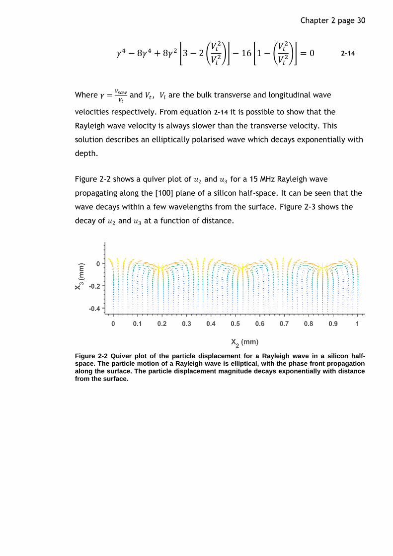
Figure 2-2 shows a quiver plot of 𝑢2 and 𝑢3 for a 15 MHz Rayleigh wave

propagating along the [100] plane of a silicon half-space. It can be seen that the

wave decays within a few wavelengths from the surface. Figure 2-3 shows the

decay of 𝑢2 and 𝑢3 at a function of distance.

Figure 2-2 Quiver plot of the particle displacement for a Rayleigh wave in a silicon half-space. The particle motion of a Rayleigh wave is elliptical, with the phase front propagation along the surface. The particle displacement magnitude decays exponentially with distance from the surface.

Chapter 2 page 31

Figure 2-3 Parallel and tangential particle displacements as a function of distance from the surface. The Majority of the energy contained within a Rayleigh is with a few wavelengths of the surface.

For Rayleigh waves on anisotropic materials the case is similar to bulk waves in

that the phase speed of the Rayleigh wave will also depend on propagation

direction along the surface. Furthermore, for most propagation directions it will

not be a pure, elliptically polarised wave, but will have a small component of

particle motion perpendicular to the sagittal plane. As with the bulk wave

equivalent these are called pseudo Rayleigh waves (Campbell & Jones 1968;

Dransfeld & Salzmann 1970).

Leaky surface waves

When 𝑋3 > 0 is occupied by a fluid the Rayleigh wave solution must be

considered both in the elastic and also the fluid medium. The form of the

equations for the Rayleigh wave in the solid medium are the same as equation

2-13 (Campbell & Jones 1969), except with addition of an attenuation factor for

the propagation of the Rayleigh wave. Such a wave is often called a ‘leaky’

surface wave due to the energy that is lost during propagation. In this case the

surface wave is losing energy to the fluid medium due to the excitation of

compressional waves and viscous damping inside the fluid.

Chapter 2 page 32 This can be considered in two parts, the transverse component of the SAW will

cause a longitudinal pressure wave to propagate into the fluid due to the

periodic density changes produced in the fluid at the boundary (Dransfeld &

Salzmann 1970) (Arzt et al. 1967). The direction of propagation of this wave will

be at the Rayleigh angle, 𝑉𝑓

𝑉𝑠𝑎𝑤= sin 𝜃𝑅. The attenuation of the leaky SAW due to

this compression wave is given by

𝛼𝑠𝑎𝑤 =

𝜌𝑓𝑉𝑓𝜌𝑠𝑉𝑠𝑎𝑤𝜆

cm−1 2-15

Here 𝜆 is the wavelength of the Rayleigh SAW . There will also be some

attenuation due to the longitudinal component of the SAW which imposes an

oscillating shearing force on the fluid. The attenuation of the SAW wave due to

this motion is (Dransfeld & Salzmann 1970)

𝛼𝑠 =

(𝜌𝑓𝜂𝜔3

2 )1/2

4𝜋2𝜌𝑠𝑉𝑠𝑎𝑤2

cm−1 2-16

It can be easily verified that 𝛼𝑠𝑎𝑤 ≫ 𝛼𝑠 and usually 𝛼𝑠 is ignored in analysis of

leaky surface waves in microfluidics e.g. (M. Alghane et al. 2012) (Michael B

Dentry et al. 2014).

Lamb waves

When the acoustic medium is a plate rather than a half-space (i.e. it occupies

the space between −ℎ

2< 𝑋3 <

ℎ

2 there are now two no-stress boundary

conditions across the top and bottom of the plate. Solutions for the wave

equation in this system are dispersive, i.e. at different frequencies the wave will

travel at different phase velocities and there can be multiple solutions (wave

modes) for a given frequency. These are known as Lamb waves after Horace

Lamb who first derived them (Lamb 1917). The Lamb wave dispersion equations

relate the Lamb wave phase velocities for a given frequency and thickness of

plate, (Rose 2014)

Chapter 2 page 33

tan (𝑞ℎ2 )

tan (𝑝ℎ2 )

= −4𝑘2𝑝𝑞

(𝑞2 − 𝑘2)2

2-17

tan (

𝑞ℎ2 )

tan (𝑝ℎ2 )

= −(𝑞2 − 𝑘2)2

4𝑘2𝑝𝑞

2-18

Where 𝑝2 =𝜔2

𝑉𝑙2 − 𝑘

2 and 𝑞2 =𝜔2

𝑉𝑡2 − 𝑘

2 with 𝑉𝑙 and 𝑉𝑡 being the longitudinal and

transverse bulk wave velocities in the medium. 𝑘 =𝜔

𝑉𝑙 where 𝑉𝑙 is the phase

velocity of the lamb wave and ℎ is the thickness of the plate. Solutions of

equation 2-17 determine the allowed wave velocities for symmetric Lamb wave

modes, and solutions of equation 2-18 determine the allowed wave velocities for

anti-symmetric wave modes.

2.2 Transmission and reflection of acoustic waves in layered media

The acoustic glucose sensor part of this thesis deals with wave reflections from a

device consisting of many layers of alternating acoustic impedance contrast. In

order to understand this, a model for acoustic reflections between all of the

layers is required. This section first introduces the theory of acoustic reflections

at a material interface. A method for calculating the total reflection and

transmission when there are many different material interfaces, the

transmission matrix method is then described.

A single boundary

In general an acoustic plane wave that is incident on a material boundary

between two isotropic, elastic mediums will partially reflect and refract at the

boundary. In addition, the reflected and refracted wave energy may take the

form of both a shear wave and a longitudinal wave.

In the general case it is appropriate to impose boundary conditions for the

particle deformation at 𝑋3 = 0 as (Ewing & Jardetzky 1957; B.A.Auld 1973b)

Chapter 2 page 34

𝐮 = 𝐮′

2-19

𝛔 ∙ 𝐧 = 𝛔′ ∙ 𝐧

2-20

These impose continuity of velocity and stress normal to the boundary. Where 𝐮

is the particle velocity for the medium inhabiting 𝑋3 < 0 and 𝐮′ for 𝑥3 > 0.

Snell’s law then applies for the refracted and reflected waves, so

1

𝑉𝑙sin𝜗𝑙 =

1

𝑉𝑡sin𝜗𝑡 =

1

𝑉𝑙′sin𝜗𝑙′ =

1

𝑉𝑡′sin𝜗𝑡′

2-21

The amplitude of the reflected and refracted waves can be derived by writing

the particle velocity fields in each medium as the sum of all reflected, refracted

and incident waves. Then by inserting these into the boundary conditions a set

of four equations is obtained. This can be solved to find the wave amplitudes for

each reflected and refracted wave using Cramer’s rule as described for example

in (B.A.Auld 1973b).

When a longitudinal wave is normally incident on a boundary, (𝜗𝑙 = 0) there are

no reflected or transmitted shear waves since the particle velocity is normal to

the boundary. The reflected and refracted compression waves will also

propagate with 𝜗𝑙 = 𝜗𝑙′ = 0. In this case there is a simple expression for the

reflection coefficient

𝛤 =

𝜌′𝑉𝑙′−𝜌𝑉𝑙

𝜌′𝑉𝑙′+𝜌𝑉𝑙 2-22

Where 𝛤 is the ratio of the incident and reflected wave amplitudes, and called

the reflection coefficient and 𝜌′ 𝑉𝑙′ are density and wave velocity for the

incidence medium and similarly 𝜌 𝑉𝑙 are for transmission medium. The

transmission coefficient is

𝑇 =

2𝜌𝑉𝑙′𝜌𝑉𝑙 + 𝜌′𝑉𝑙′

2-23

Chapter 2 page 35

The product 𝜌𝑉𝑙 is often referred to as the characteristic acoustic impedance

and represented in equations with the symbol 𝑍𝑖𝑚𝑝.

When one side of the half-space is replaced with a fluid the scattering equations

are somewhat simplified because the fluid cannot support a shear wave and 𝑉𝑡 →

0, correspondingly the shear stress at the boundary must be zero from the

boundary conditions above. For the case of an incident compression wave in the

fluid a refracted shear and compression wave can be excited in the solid, as well

as a reflected compression wave in the fluid. The reflection and refraction

coefficients can be expressed exactly as in (Ewing & Jardetzky 1957). Again

when the incident compression wave is normal to the boundary i.e. 𝜗𝑙 = 0, there

are no scattered shear waves and the reflected and refracted compression waves

obey the reflection and transmission coefficients in equation 2-22 and 2-23.

Reflections at many boundaries

When there is more than one parallel boundary the number of reflected and

refracted waves in each medium contains rapidly more terms. For example

consider an isotropic elastic solid plate with plane parallel sides suspended in a

water bath. A compression wave in the fluid medium is incident on the left side

of the plate so that 𝜗𝑙 = 0. In this case there are no shear waves generated and

all the reflected and refracted waves propagate normal to the boundary, with

reflection coefficients obeying equations 2-22 and 2-23. The sum of all the

waves on the left hand side of the plate is therefore the sum of the incident

wave, the reflection from the first boundary with the solid, the transmission

through the first boundary which reflects off the second boundary comes back

and transmits through the first boundary, and so on to infinity. This can be

expressed as, (Brekhovskikh 1960)

𝛤12+𝑇12𝑇21𝛤23𝑒2𝑖𝑘2𝑑∑[𝛤23𝛤21𝑒

2𝑖𝑘2𝑑]𝑛

∞

𝑛=0

2-24

Chapter 2 page 36

Where 𝛤12 , 𝛤23 , 𝛤21 and 𝑇12, 𝑇21 are the reflection coefficients and transmission

coefficients for the boundaries between regions 1 2 and 3 where region 1 are 3

are the water to the left and right side of the plate and region 2 is the elastic

plate. 𝑑 is the thickness of the plate and 𝑘2 is the wavenumber in the plate. The

effective reflection coefficient of the two boundaries taken together will simply

be the ratio of the incident wave with equation 2-24,

𝛤 =

𝛤23 + 𝛤12𝑒2𝑖𝑘2𝑑

1 + 𝛤23𝛤12𝑒2𝑖𝑘2𝑑

2-25

For a plate of half wavelength thickness where

𝑑 = 𝑚𝜆

2 , i. e. 2𝑘2𝑑 = 2𝜋𝑚, 𝑚 = 1,2,… 2-26

equation 2-25 becomes 𝛤 = 0, i.e. it is as if the plate is not there at all and the

wave energy is completely transmitted. For an oblique incidence a similar case

for complete transmission exists, except this time 2𝑘2𝑑𝑐𝑜𝑠𝜗2 = 2𝜋𝑚

(Brekhovskikh 1960).

The chain matrix technique can be used to find the reflection and transmission

coefficient for a system of n parallel layers. This was first applied to acoustic

wave propagation in layered media by (Thomson 1950). This method uses a

transfer matrix to relate the stress and displacements at the top of a layer with

those at the bottom. For the simplest case of a normally incident wave in a ‘1D’

layered structure there can only be two compression waves, one going forwards

and one going backwards. In this case the particle velocity and stress fields can

be reduced to one direction component normal to the layers, say the 𝑋

direction. Then if the particle velocity and stress at the bottom of one layer are

known then they can be deduced at the top using the transfer matrix, (Oakley

1997)

[𝜎𝑋𝑢𝑋] = [

cosh (𝑘𝑙) 𝑍sinh(𝑘𝑙)

sinh (𝑘𝑙)

𝑍𝑖𝑚𝑝cosh (𝑘𝑙)

] [𝜎𝑋+𝑙𝑢𝑋+𝑙

] 2-27

Chapter 2 page 37

Where 𝑘 Is the wavenumber, 𝑙 is the thickness of the layer, Zimp is the acoustic

impedance of the layer 𝜎𝑋 is the stress at the layer boundary and 𝑢𝑋 is the

particle velocity at the layer boundary. [𝜎𝑋𝑢𝑋] then becomes the input for the next

layer, for which a propagation matrix relates the top and bottom. The transfer

matrix for an arbitrary number of layers can then be coupled together to get a

single matrix for the whole system. For example a two layer system would be

[𝜎𝑙1𝑢𝑙1] = [

cosh (𝑘1𝑙1) 𝑍𝑙1sinh(𝑘1𝑙1)

sinh (𝑘1𝑙1)

𝑍𝑖𝑚𝑝1cosh (𝑘1𝑙1)

] [

cosh (𝑘2𝑙2) 𝑍2sinh(𝑘2𝑙2)

sinh (𝑘2𝑙2)

𝑍𝑖𝑚𝑝2cosh (𝑘2𝑙2)

] [𝜎2+𝑙𝑢2+𝑙

]

2-28

Additional layers simply result in additional multiplication steps. This can be

reduced to one single transfer matrix,

[𝜎𝑙1𝑢𝑙1] = [

𝑚11 𝑚12

𝑚21 𝑚22] [𝜎𝑛+𝑙𝑢𝑛+𝑙

]

2-29

Where 𝑛 refers to the ‘nth’ layer or the last layer in the system. Wave

attenuation through each layer can be included by specifying a complex

wavenumber, e.g. 𝑘 = 𝑖𝛼 +2𝜋

𝜆𝑋 (Oakley 1997).

The effective reflection coefficient from all the layers can be then calculated,

assuming a wave incident from infinity (from a non-reflecting medium) on the

layers (Oakley 1997)

𝑅 =

𝑍𝑖𝑚𝑝0 − 𝑍𝑖𝑚𝑝𝑀𝑍𝑖𝑚𝑝0 + 𝑍𝑖𝑚𝑝𝑀

2-30

Where 𝑍𝑖𝑚𝑝0 is the acoustic impedance of the medium the acoustic wave is

incident on and

𝑍𝑖𝑚𝑝𝑀 =

𝑍𝑖𝑚𝑝𝑓𝑚22 −𝑚12

𝑚11 − 𝑍𝑖𝑚𝑝𝑓𝑚21 2-31

Chapter 2 page 38

Where 𝑍𝑖𝑚𝑝𝑓 is the acoustic impedance of the final medium. The phase and

group delay of the reflected waves can also be calculated,

𝜑 = cos−1 (

𝑅𝑒(𝑅)

√𝑅𝑒(𝑅)2+𝐼𝑚(𝑅)2)

2-32

𝜏𝑔(𝜔) = −

𝑑𝜑(𝜔)

𝑑𝜔

2-33

Where 𝜑 and 𝜏𝑔stand for phase and group delay respectively.

This method assumes plane wave propagation and is ‘1D’ in the sense that it

allows for variation only in the one dimension along the layers. The chain matrix

technique can also be extended to two dimensions, which then includes the

effect of incidence angle and propagating shear waves. This greatly increases

the complexity of the transfer matrix, which now has to describe the

propagation of four waves, two compression and two shear waves travelling in

opposite directions (Lowe 1995).

2.3 Piezoelectricity and ultrasonic transducers

Two different types of ultrasonic transducer are used in this thesis to create the

ultrasonic fields of interest. Both of these methods rely on the piezoelectric

effect to transduce an electric field into an acoustic field. The theory of this is

therefore introduced here first. Then there is a brief introduction to

interdigitated transducers that were used here to generate surface acoustic

waves. After this thickness mode ultrasonic transducers that were used in this

thesis to create a plane longitudinal wave for the acoustic glucose sensor

experiments are introduced. A KLM equivalent circuit model of a thickness mode

ultrasonic transducer was used to model the output from the transducer used in

these experiments. The theory of this also is developed here.

Chapter 2 page 39

Piezoelectricity

Piezoelectricity is a feature of a class of materials where an electric field in the

material is generated by the initiation of a deformation. The reverse is also true,

i.e. an applied electric field will produce a mechanical deformation. The origin

of the piezoelectric effect is in the particular microscopic distribution of charges

in the material, a macroscopic deformation changes the spatial distribution of

these charges with can lead a change in the electric field across the material. An

asymmetric charge distribution can lead to piezoelectricity in materials however

a symmetric charge distribution can never lead to piezoelectricity. For this

reason piezoelectric materials must always be anisotropic materials.

For infinitesimally small changes in mechanical and electrical loads a simplified

set of linear equations can be used to describe the motion of piezoelectric

materials. This is usually reasonable when considering acoustic waves generated

by a transducer etc. Equation 2-1 can then be rewritten as, (Yang 2005)

𝜎𝑖𝑗 = 𝑐𝑖𝑗𝑘𝑙𝐸 휀𝑘𝑙 − 𝑒𝑘𝑖𝑗𝐸𝑘

2-34

Here ijklEc is the stiffness tensor at a constant electric field E. kije is called the

piezoelectric tensor which relates the resulting stress from an applied electric

field. The electric displacement must also be rewritten as

𝐷𝑖 = 𝜉𝑖𝑗

𝜀 𝐸𝑗 + 𝑒𝑖𝑗𝑘𝑙휀𝑗𝑘 2-35

Where 𝜉𝑖𝑗𝜀 is the permittivity tensor for constant strain. The equation of motion

becomes

𝜌𝑑2𝑢𝑖𝑑𝑡2

= 𝑒𝑘𝑖𝑗𝜕2𝜑

𝜕𝑋𝑗𝜕𝑋𝑘+∑𝐶𝑖𝑗𝑘𝑙

𝐸𝜕2𝑢𝑘𝜕𝑋𝑗𝜕𝑋𝑙

𝑙

2-36

Where a quasi-static approximation for the electric field is used since electric

disturbances travel much faster than mechanical ones. If the material is an

insulator then ∇ ∙ 𝐷 = 0 and the electric potential 𝜑 can be written in terms of 𝐮

Chapter 2 page 40

휀𝑖𝑗𝑠

∂2𝜑

∂𝑋𝑖 ∂𝑋𝑗=∑eljk

∂2𝑢𝑗∂𝑋𝑖 ∂𝑋𝑘

k

2-37

Finding the acoustic wave solutions for piezoelectric materials involves solving

these four equations for 1u 2u 3u and 𝜑. For an acoustic wave propagating

through the material there is now an accompanying electric potential which

must also take a waveform so that for the case of Rayleigh surface waves

propagating on a piezoelectric half space the particle displacements will have

the same form as equation 2-13 and the electric potential will similarly be

𝜑 = 𝛽4𝑒

−𝑘𝛼4𝑋3+𝑖𝑘(𝑋1−𝑉𝑠𝑎𝑤𝑡) 2-38

Inter-digitated transducers for SAW generation

Piezoelectric materials provide the ability to create an interface between

electric and acoustic waves which allows for the generation and detection of

acoustic signals using electronics. Depending on the direction of the applied

field relative to the material different acoustic waves modes can be excited. A

common method for exciting and detecting Rayleigh waves is via the use of an

inter-digitated transducer or IDT for short (White & Voltmer 1965). An IDT is a

pattern of inter-locking fingers as shown in Figure 2-4 which is usually applied as

a thin metal film deposited onto the surface of a piezoelectric material.

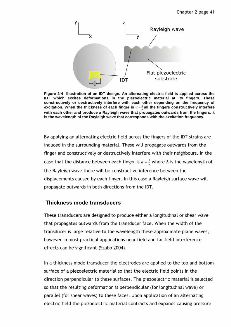
Chapter 2 page 41

Figure 2-4 Illustration of an IDT design. An alternating electric field is applied across the IDT which excites deformations in the piezoelectric material at its fingers. These constructively or destructively interfere with each other depending on the frequency of

excitation. When the thickness of each finger is 𝒅 =𝝀

𝟒 all the fingers constructively interfere

with each other and produce a Rayleigh wave that propagates outwards from the fingers. 𝝀 is the wavelength of the Rayleigh wave that corresponds with the excitation frequency.

By applying an alternating electric field across the fingers of the IDT strains are

induced in the surrounding material. These will propagate outwards from the

finger and constructively or destructively interfere with their neighbours. In the

case that the distance between each finger is 𝑑 =𝜆

4 where λ is the wavelength of

the Rayleigh wave there will be constructive inference between the

displacements caused by each finger. In this case a Rayleigh surface wave will

propagate outwards in both directions from the IDT.

Thickness mode transducers

These transducers are designed to produce either a longitudinal or shear wave

that propagates outwards from the transducer face. When the width of the

transducer is large relative to the wavelength these approximate plane waves,

however in most practical applications near field and far field interference

effects can be significant (Szabo 2004).

In a thickness mode transducer the electrodes are applied to the top and bottom

surface of a piezoelectric material so that the electric field points in the

direction perpendicular to these surfaces. The piezoelectric material is selected

so that the resulting deformation is perpendicular (for longitudinal wave) or

parallel (for shear waves) to these faces. Upon application of an alternating

electric field the piezoelectric material contracts and expands causing pressure

Chapter 2 page 42 waves to propagate through the material. When frequency of the electric field

coincides with,

𝑓 =

𝑚𝑉

2𝑑

2-39

Where 𝑑 is the thickness of the transducer and 𝑉 is the speed of sound in the

piezoelectric element, and 𝑚 = 1,3,5, … etc, there is a peak in the output of the

transducer. This is the condition for the waves propagating through the

transducer to all constructively interfere with each other (Szabo 2004).

KLM equivalent circuit for transducer modelling

The electrical response of a thickness mode transducer can be effectively

described using an equivalent circuit model. This describes the transducer as a

series of elements in an electric delay line with the acoustic part modelled using

equivalent analogous elements. This was first introduced by (Mason 1969) and

then further developed by (Krimholtz et al. 1970). Each element is represented

by a transfer matrix analogous with the transfer matrices used to model acoustic

wave reflections. Figure 2-5 illustrates the equivalent circuit model.

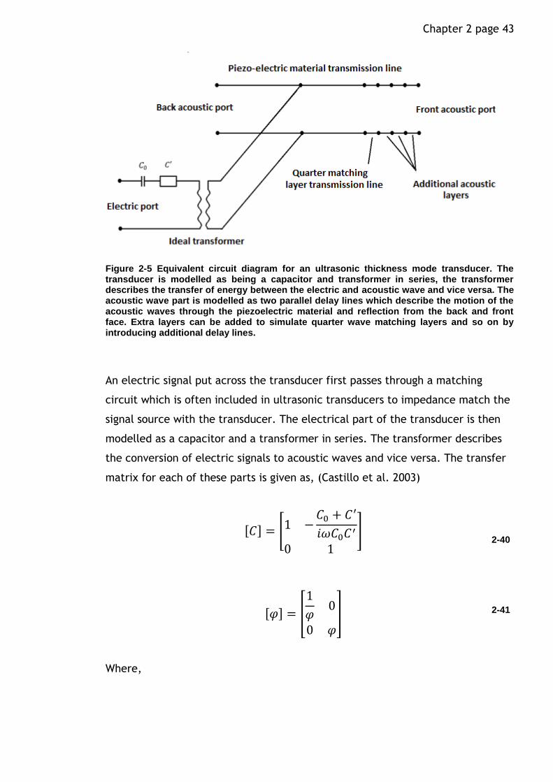
Chapter 2 page 43

Figure 2-5 Equivalent circuit diagram for an ultrasonic thickness mode transducer. The transducer is modelled as being a capacitor and transformer in series, the transformer describes the transfer of energy between the electric and acoustic wave and vice versa. The acoustic wave part is modelled as two parallel delay lines which describe the motion of the acoustic waves through the piezoelectric material and reflection from the back and front face. Extra layers can be added to simulate quarter wave matching layers and so on by introducing additional delay lines.

An electric signal put across the transducer first passes through a matching

circuit which is often included in ultrasonic transducers to impedance match the

signal source with the transducer. The electrical part of the transducer is then

modelled as a capacitor and a transformer in series. The transformer describes

the conversion of electric signals to acoustic waves and vice versa. The transfer

matrix for each of these parts is given as, (Castillo et al. 2003)

[𝐶] = [1 −𝐶0 + 𝐶

′

𝑖𝜔𝐶0𝐶′

0 1

]

2-40

[𝜑] = [

1

𝜑0

0 𝜑]

2-41

Where,

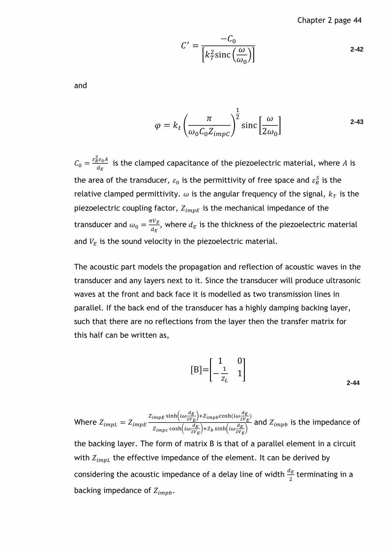
Chapter 2 page 44

𝐶′ =−𝐶0

[𝑘𝑇2sinc (

𝜔𝜔0)]

2-42

and

𝜑 = 𝑘𝑡 (𝜋

𝜔0𝐶0𝑍𝑖𝑚𝑝𝐶)

12

sinc [𝜔

2𝜔0]

2-43

𝐶0 =𝜀𝑅𝑆𝜀0𝐴

𝑑𝐸 is the clamped capacitance of the piezoelectric material, where 𝐴 is

the area of the transducer, 휀0 is the permittivity of free space and 휀𝑅𝑆 is the

relative clamped permittivity. 𝜔 is the angular frequency of the signal, 𝑘𝑇 is the

piezoelectric coupling factor, 𝑍𝑖𝑚𝑝𝐸 is the mechanical impedance of the

transducer and 𝜔0 =𝜋𝑉𝐸

𝑑𝐸, where 𝑑𝐸 is the thickness of the piezoelectric material

and 𝑉𝐸 is the sound velocity in the piezoelectric material.

The acoustic part models the propagation and reflection of acoustic waves in the

transducer and any layers next to it. Since the transducer will produce ultrasonic

waves at the front and back face it is modelled as two transmission lines in

parallel. If the back end of the transducer has a highly damping backing layer,

such that there are no reflections from the layer then the transfer matrix for

this half can be written as,

[B]=[

1 0

−1

𝑍𝐿1]

2-44

Where 𝑍𝑖𝑚𝑝𝐿 = 𝑍𝑖𝑚𝑝𝐸𝑍𝑖𝑚𝑝𝐸 sinh(𝑖𝜔

𝑑𝐸2𝑉𝐸

)+𝑍𝑖𝑚𝑝𝑏cosh (𝑖𝜔𝑑𝐸2𝑉𝐸

)

𝑍𝑖𝑚𝑝𝑐 cosh(𝑖𝜔𝑑𝐸2𝑉𝐸

)+𝑍𝑏 sinh(𝑖𝜔𝑑𝐸2𝑉𝐸

) and 𝑍𝑖𝑚𝑝𝑏 is the impedance of

the backing layer. The form of matrix B is that of a parallel element in a circuit

with 𝑍𝑖𝑚𝑝𝐿 the effective impedance of the element. It can be derived by

considering the acoustic impedance of a delay line of width 𝑑𝐸

2 terminating in a

backing impedance of 𝑍𝑖𝑚𝑝𝑏.

Chapter 2 page 45 The transfer matrix for the front half of the transducer layer is just

[𝑇1] =

[ cosh (𝑖𝜔

𝑑𝐸2𝑉𝐸

) −𝑍𝑖𝑚𝑝𝐸sinh (𝑖𝜔𝑑𝐸2𝑉𝐸

)

−sinh (𝑖𝜔

𝑑𝐸2𝑉𝐸

)

𝑍𝑖𝑚𝑝𝐸cosh (𝑖𝜔

𝑑𝐸2𝑉𝐸

)]

2-45

Similar transfer matrices can be written for other acoustic layers, for example a

quarter wave matching layer, by replacing 𝑑𝐸 with the layer thickness and 𝑉𝐸

and 𝑍𝑖𝑚𝑝𝐸 with the velocity and impedance of the layer. Reflection and

transmission coefficients of the transducer can then be deduced for the

transducer in an exactly similar method to that described in equation 2-28, i.e.

the transfer matrices are multiplied together and the coefficients deduced from

the input and output impedance, the input impedance now being the electric

impedance of the electric input port. Damping can also be included by using a

complex wave vector as in the acoustic analogy.

2.4 Acoustic streaming

The section introduces the theory behind acoustic streaming focusing especially

on streaming due to leaky SAWs.

Acoustic streaming background

As discussed previously fluids have the capacity to flow and permanently change

shape when deformed, which distinguishes them from elastic solid materials.

This leads to different equations describing the motion of a fluid through time,

i.e. the Navier Stokes equation. In turn this leads to different acoustic

phenomena, for example shear waves in a fluid are diffusive, and decay within a

very short distance. Another example of the differences between fluids and

solids is the acoustic streaming phenomena that can exist in fluids. In this case

an acoustic beam in the fluid or on the boundary between the fluid and another

material can produce a steady flow.

The physical origins of acoustic streaming can be derived analytically using the

method of successive approximations to solve the Navier-Stokes equation

Chapter 2 page 46 (Nyborg 1965). The equation is first solved for the sound field in the fluid,

assuming a sinusoidal velocity field. Then an additional term which is assumed to

be a time constant streaming velocity is added and the Navier stokes equation is

solved again. The velocity, pressure and density are described by,

𝐩 = 𝐩𝟎 + 𝐩𝟏 + 𝐩𝟐

𝜌 = 𝜌0 + 𝜌1 + 𝜌2

𝐮 = 𝐮𝟎 + 𝐮𝟏 + 𝐮𝟐

2-46

The zero order term refers to the properties of the fluid at rest, where 𝑢0 is zero

and 𝜌0 and 𝑝0 are the hydrostatic pressure and density. The first order term

describes the sound field which will oscillate with frequency 𝜔. The second

order term is the steady streaming component and is therefore time

independent. This method is only accurate when 𝐮𝟐 ≪ 𝐮𝟏 and this restricts the

analysis to small amplitude sound waves – slow streaming.(Friend & Yeo 2011). It

can be shown that the body force on the fluid due to the sound field is then,

𝐅𝐛 = 𝜌0⟨𝐮𝟏 ∙ ∇𝐮𝟏 + 𝐮𝟏∇ ∙ 𝐮𝟏⟩ 2-47

From equation 2-47 different streaming phenomena can be described depending

on what kind of sound field and boundary conditions act on the fluid.

An example of acoustic streaming by a plane wave.

A plane wave propagating through a boundless fluid is possibly the simplest to

consider. Assuming a sound field of the form, (Nyborg 1965)

𝑢𝑋 = 𝐴𝑒−𝛼𝑋cos (𝜔𝑡 − 𝑘𝑋)

2-48

Where the particle velocity is confined to one axis and the vector notation has

been dropped, 𝛼 represents the attenuation coefficient of the wave and 𝐴 is the

initial velocity amplitude. The body force on the fluid can then be calculated as,

Chapter 2 page 47 𝐹𝑏 = 𝜌0𝛼𝐴

2𝑒−2𝛼𝑋

2-49

Which points in the direction of propagation of the sound beam, with magnitude

proportional to 𝛼 and the initial amplitude of the particle velocity, 𝐴. This is

often called Eckhart streaming or bulk streaming as it is found within the bulk of

fluids where 𝑢1 can be described as above.

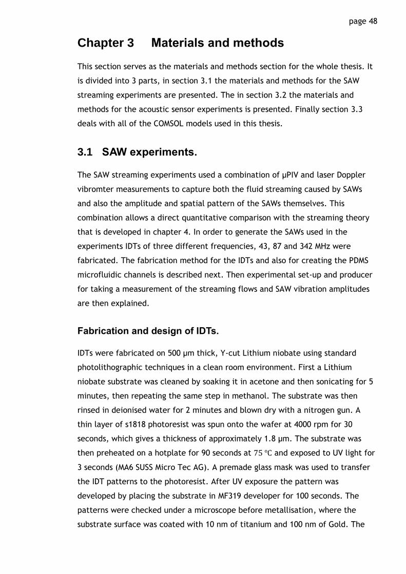
Chapter 3 page 48

Chapter 3 Materials and methods

This section serves as the materials and methods section for the whole thesis. It

is divided into 3 parts, in section 3.1 the materials and methods for the SAW

streaming experiments are presented. The in section 3.2 the materials and

methods for the acoustic sensor experiments is presented. Finally section 3.3

deals with all of the COMSOL models used in this thesis.

3.1 SAW experiments.

The SAW streaming experiments used a combination of µPIV and laser Doppler

vibromter measurements to capture both the fluid streaming caused by SAWs

and also the amplitude and spatial pattern of the SAWs themselves. This

combination allows a direct quantitative comparison with the streaming theory

that is developed in chapter 4. In order to generate the SAWs used in the

experiments IDTs of three different frequencies, 43, 87 and 342 MHz were

fabricated. The fabrication method for the IDTs and also for creating the PDMS

microfluidic channels is described next. Then experimental set-up and producer

for taking a measurement of the streaming flows and SAW vibration amplitudes

are then explained.

Fabrication and design of IDTs.

IDTs were fabricated on 500 μm thick, Y-cut Lithium niobate using standard

photolithographic techniques in a clean room environment. First a Lithium

niobate substrate was cleaned by soaking it in acetone and then sonicating for 5

minutes, then repeating the same step in methanol. The substrate was then

rinsed in deionised water for 2 minutes and blown dry with a nitrogen gun. A

thin layer of s1818 photoresist was spun onto the wafer at 4000 rpm for 30

seconds, which gives a thickness of approximately 1.8 μm. The substrate was

then preheated on a hotplate for 90 seconds at 75 ℃ and exposed to UV light for

3 seconds (MA6 SUSS Micro Tec AG). A premade glass mask was used to transfer

the IDT patterns to the photoresist. After UV exposure the pattern was

developed by placing the substrate in MF319 developer for 100 seconds. The

patterns were checked under a microscope before metallisation, where the

substrate surface was coated with 10 nm of titanium and 100 nm of Gold. The

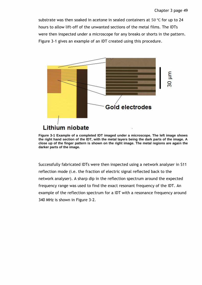
Chapter 3 page 49 substrate was then soaked in acetone in sealed containers at 50 ℃ for up to 24

hours to allow lift-off of the unwanted sections of the metal films. The IDTs

were then inspected under a microscope for any breaks or shorts in the pattern.

Figure 3-1 gives an example of an IDT created using this procedure.

Figure 3-1 Example of a completed IDT imaged under a microscope. The left image shows the right hand section of the IDT, with the metal layers being the dark parts of the image. A close up of the finger pattern is shown on the right image. The metal regions are again the darker parts of the image.

Successfully fabricated IDTs were then inspected using a network analyser in S11

reflection mode (i.e. the fraction of electric signal reflected back to the

network analyser). A sharp dip in the reflection spectrum around the expected

frequency range was used to find the exact resonant frequency of the IDT. An

example of the reflection spectrum for a IDT with a resonance frequency around

340 MHz is shown in Figure 3-2.

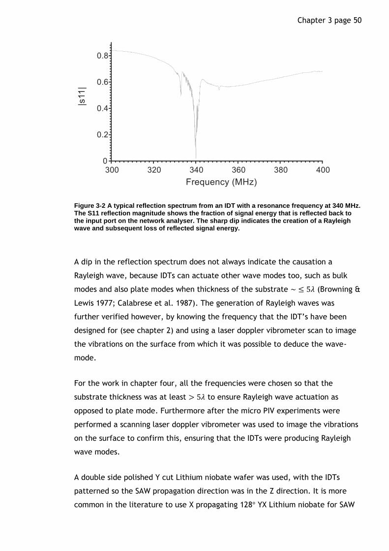
Chapter 3 page 50

Figure 3-2 A typical reflection spectrum from an IDT with a resonance frequency at 340 MHz. The S11 reflection magnitude shows the fraction of signal energy that is reflected back to the input port on the network analyser. The sharp dip indicates the creation of a Rayleigh wave and subsequent loss of reflected signal energy.

A dip in the reflection spectrum does not always indicate the causation a

Rayleigh wave, because IDTs can actuate other wave modes too, such as bulk

modes and also plate modes when thickness of the substrate ~ ≤ 5𝜆 (Browning &

Lewis 1977; Calabrese et al. 1987). The generation of Rayleigh waves was

further verified however, by knowing the frequency that the IDT’s have been

designed for (see chapter 2) and using a laser doppler vibrometer scan to image

the vibrations on the surface from which it was possible to deduce the wave-

mode.

For the work in chapter four, all the frequencies were chosen so that the

substrate thickness was at least > 5𝜆 to ensure Rayleigh wave actuation as

opposed to plate mode. Furthermore after the micro PIV experiments were

performed a scanning laser doppler vibrometer was used to image the vibrations

on the surface to confirm this, ensuring that the IDTs were producing Rayleigh

wave modes.

A double side polished Y cut Lithium niobate wafer was used, with the IDTs

patterned so the SAW propagation direction was in the Z direction. It is more

common in the literature to use X propagating 128° YX Lithium niobate for SAW

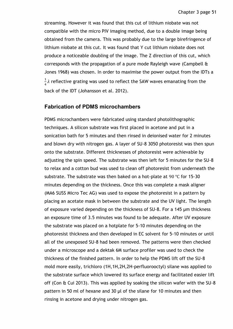
Chapter 3 page 51 streaming. However it was found that this cut of lithium niobate was not

compatible with the micro PIV imaging method, due to a double image being

obtained from the camera. This was probably due to the large birefringence of

lithium niobate at this cut. It was found that Y cut lithium niobate does not

produce a noticeable doubling of the image. The Z direction of this cut, which

corresponds with the propagation of a pure mode Rayleigh wave (Campbell &

Jones 1968) was chosen. In order to maximise the power output from the IDTs a

1

4𝜆 reflective grating was used to reflect the SAW waves emanating from the

back of the IDT (Johansson et al. 2012).

Fabrication of PDMS microchambers

PDMS microchambers were fabricated using standard photolithographic

techniques. A silicon substrate was first placed in acetone and put in a

sonication bath for 5 minutes and then rinsed in deionised water for 2 minutes

and blown dry with nitrogen gas. A layer of SU-8 3050 photoresist was then spun

onto the substrate. Different thicknesses of photoresist were achievable by

adjusting the spin speed. The substrate was then left for 5 minutes for the SU-8

to relax and a cotton bud was used to clean off photoresist from underneath the

substrate. The substrate was then baked on a hot-plate at 90 ℃ for 15-30

minutes depending on the thickness. Once this was complete a mask aligner

(MA6 SUSS Micro Tec AG) was used to expose the photoresist in a pattern by

placing an acetate mask in between the substrate and the UV light. The length

of exposure varied depending on the thickness of SU-8. For a 145 μm thickness

an exposure time of 3.5 minutes was found to be adequate. After UV exposure

the substrate was placed on a hotplate for 5-10 minutes depending on the

photoresist thickness and then developed in EC solvent for 5-10 minutes or until

all of the unexposed SU-8 had been removed. The patterns were then checked

under a microscope and a dektak 6M surface profiler was used to check the

thickness of the finished pattern. In order to help the PDMS lift off the SU-8

mold more easily, trichloro (1H,1H,2H,2H-perfluorooctyl) silane was applied to

the substrate surface which lowered its surface energy and facilitated easier lift

off (Con & Cui 2013). This was applied by soaking the silicon wafer with the SU-8

pattern in 50 ml of hexane and 30 μl of the silane for 10 minutes and then

rinsing in acetone and drying under nitrogen gas.

Chapter 3 page 52 The PDMS microchambers were then made by mixing the silicone elastomer base

in a 1:10 ratio with the curing agent before depositing in a desiccator to degass

for 15 minutes. The mixture was then carefully poured onto patterns and left to

cure for 4 hours in a 70 °C oven. The cured PDMS with the microfluidic patterns

was then cut out using a scalpel. An inlet well and an outlet well were punched

into the PDMS using a disposable biopsy dermal punch.

In order to get a fluid sample into the microchannels the PDMS was first placed

onto the lithium niobate and aligned with the IDT and SAW beam propagation

path. The PDMS and lithium niobate formed a weak reversible bond, which was

just enough to keep a fluid contained within the microchannel structure without

leaking. Since the PDMS was naturally hydrophobic it was placed in an oxygen

plasma asher for 30 seconds at 30 W (Bodas & Khan-Malek 2007). This made the

PDMS more hydrophilic where it was in contact with the oxygen plasma, i.e. the

channels and the outer edges of the PDMS but not the part in contact with the

lithium niobate. This allowed a fluid sample to wick along the microchannels but

not leak by seeping in between the PDMS and lithium niobate. This method was

considered preferable over permanent bonding of the PDMS to the substrate

which is the common method in the literature because it allowed the IDT to be

reused after the experiment (Destgeer et al. 2013; Luong et al. 2010).

Experimental set-up and channel network design.

The channel network design and the path of the SAW beam relative to the

channel network is shown in Figure 3-3. This shows the experimental set-up

before a fluid sample has been inserted at the inlet well, where PDMS is

indicated by the transparent grey region. Once the fluid had been inserted it

flowed from the inlet to outlet well through the square shaped chamber, a thin

100 µm thick wall stopped it from penetrating the dry channel indicated on the

diagram. The PIV measurements were performed in the square shaped chamber

which had dimensions of 400 by 400 by 150 µm (X, Y, Z).

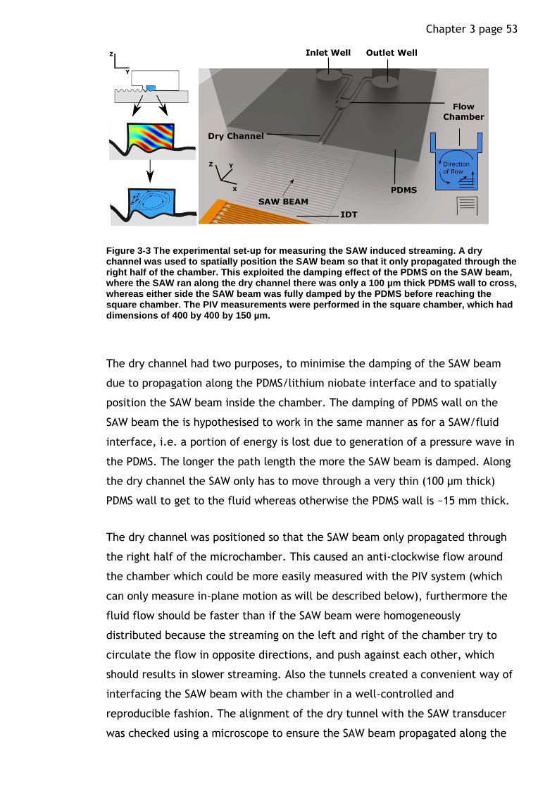
Chapter 3 page 53

Figure 3-3 The experimental set-up for measuring the SAW induced streaming. A dry channel was used to spatially position the SAW beam so that it only propagated through the right half of the chamber. This exploited the damping effect of the PDMS on the SAW beam, where the SAW ran along the dry channel there was only a 100 µm thick PDMS wall to cross, whereas either side the SAW beam was fully damped by the PDMS before reaching the square chamber. The PIV measurements were performed in the square chamber, which had dimensions of 400 by 400 by 150 µm.

The dry channel had two purposes, to minimise the damping of the SAW beam

due to propagation along the PDMS/lithium niobate interface and to spatially

position the SAW beam inside the chamber. The damping of PDMS wall on the

SAW beam the is hypothesised to work in the same manner as for a SAW/fluid

interface, i.e. a portion of energy is lost due to generation of a pressure wave in

the PDMS. The longer the path length the more the SAW beam is damped. Along

the dry channel the SAW only has to move through a very thin (100 µm thick)

PDMS wall to get to the fluid whereas otherwise the PDMS wall is ~15 mm thick.

The dry channel was positioned so that the SAW beam only propagated through

the right half of the microchamber. This caused an anti-clockwise flow around

the chamber which could be more easily measured with the PIV system (which

can only measure in-plane motion as will be described below), furthermore the

fluid flow should be faster than if the SAW beam were homogeneously

distributed because the streaming on the left and right of the chamber try to

circulate the flow in opposite directions, and push against each other, which

should results in slower streaming. Also the tunnels created a convenient way of

interfacing the SAW beam with the chamber in a well-controlled and

reproducible fashion. The alignment of the dry tunnel with the SAW transducer

was checked using a microscope to ensure the SAW beam propagated along the

Chapter 3 page 54 tunnel. The PDMS slab was repositioned if the alignment was off by more than

1°.

Laser Doppler vibrometer measurements

A laser Doppler vibrometer (LDV, Polytec Inc) was used to measure the

amplitude of the SAWs used in the micro PIV experiments. This worked by

measuring the Doppler shift of a laser beam focussed onto a spot on the surface.

By scanning along the surface a profile of the SAW beam could be put together,

the SAWs could effectively be ‘imaged’. Since relatively high frequency SAWs

were used in the streaming study, corresponding to short wavelengths, a 50 X

objective lens was used to focus the laser beam tightly enough to spatially

resolve the vibrations.

PIV measurements

Particle image velocimetry (PIV) is a method which can be used to obtain

quantitative information about the flow velocity field of a fluid. Tracer

particles, which will move with the fluid are imaged at different times and the

velocity of the particles deduced from the distance they have travelled between

each frame. PIV is a widely used technique and different technical arrangements

and considerations are necessary for the wide variety of different length scales

that there is interest in measuring over.

Efforts to investigate fluid flow in microfluidic structures have necessarily led to

the use of small particles and microscopy to properly resolve the flow. In turn

these require florescence techniques and high powered pulsed lasers to be able

to image the particles and capture fast flows (above 1 mms-1) with a sufficient

time resolution (Meinhart et al. 1999).

A micro PIV imaging system from TSI was used to measure the leaky SAW flows.

A transparent Lithium niobate wafer with the microchamber positioned on top

was placed over a microscope objective and a high power pulsed laser was used

to image a focal plane in the chamber. A high frame rate camera captured

images of the particles in the flow. Insight 4G was used to coordinate the laser

pulsing and the camera trigger and calculate the flow velocities. The laser

Chapter 3 page 55 pulsing was timed so that the time period for each frame on the camera

coincided with a laser pulse. A pair of frames then shows the position of

particles at the time of each laser pulse.

The flow fields were calculated by comparing the position of particles between a

pair of images. The image is split up into a square grid where particle

displacement in each square of the grid (interrogation spot) was compared

between the frames. A correlation technique was then used calculate the flow

velocity in each spot, see (Raffel & Wereley 2007) for more details on this

technique. The size of the interrogation spot needs to be big enough that there

are sufficient number particles in the spot to make an accurate measurement

and yet small enough that the spatial variation in the fluid flow over the spot is

not unacceptably large. There are some basic rules of thumb for selecting the

size of the interrogation spot. There should be at least 10 particles in the

interrogation spot. The total particle displacement should be no more than 0.25

times the integration spot length to ensure that no too many particles leave the

spot. The total out of plane particle displacement should be no more than 0.25

times the correlation depth (discussed in next few paragraphs). The fluid flow

velocity in the interrogation spot can be assumed to be invariant.

For measuring microfluidic flows achieving sufficient particle density can be

quite difficult in practice. An ensemble correlation technique can be used to

improve the accuracy of a measurement when low-particle seeding density is

unavoidable. This averages the correlation of many pairs of images to improve

the total number of particles in each interrogation spot. An ensemble correlation

of at least 20 image pairs were used in this work to ensure there were enough

particles in each spot, while the frame and laser pulse rate was adjusted so that

the total particle displacement was not too large.

1 μm diameter fluorescent polymer microspheres (Bangs Laboratories Inc) were

used as the tracer particles. These were found to give a reasonable fluorescent

signal for their size. Smaller particles were found to be very difficult to image at

the faster frame rate required when imaging the SAW flows at higher input

powers. Polymer microspheres also have a very similar density to water so they

move with the flow of the water faithfully. The response time for a particle

Chapter 3 page 56 subjected to a step change in the local fluid velocity can be calculated from

(Raffel & Wereley 2007)

𝜏𝑝 =𝑑𝑝2𝜌

18𝜇 3-1

Where 𝑑𝑝 is the particle diameter, 𝜌 is the density and 𝜇 is the dynamic viscosity

of the fluid. This gives an estimate of how much the particle will lag behind the

fluid. For the spheres used in this work 𝜏𝑝~10−8 s, much smaller than the time

scales for any realistic Leaky SAW induced flow.

It is not possible to image out of plane motion with this technique, however it is

possible to image the in plane motion at different depths in the chamber by

adjusting the focal positon of the objective lens. This way slices of the flow field

at different depths in the chamber can be observed. The correlation depth is

defined as the distance from the focal plane where a particle will contribute less

than 1% to the overall correlation function, based on considering the depth of

field of the objective lens. The depth of correlation is given by (Raffel &

Wereley 2007),

𝛿𝑐𝑔 =3𝑛𝜆0

𝑁𝐴2 3-2

A Nikon 10X CFI plan Fluor objective was used as the objective lens, this gives a

depth of correlation of 𝛿𝑐𝑔 = 23 μm.

It is known that SAW streaming flows in droplets take a few hundred milliseconds

to come to equilibrium after the SAW beam is first applied. (Alghane 2013) In

order to check how long it takes to come to equilibrium in the microchambers,

images were recorded before and after SAW application at different input

powers. Figure 3-4 shows the mean velocity in the chamber against time. When

the SAW beam is activated the flow rapidly rises to an equilibrium over a period

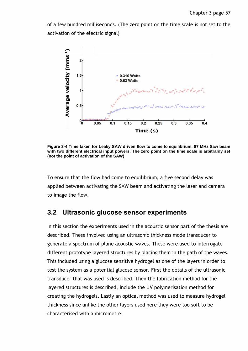
Chapter 3 page 57 of a few hundred milliseconds. (The zero point on the time scale is not set to the

activation of the electric signal)

Figure 3-4 Time taken for Leaky SAW driven flow to come to equilibrium. 87 MHz Saw beam with two different electrical input powers. The zero point on the time scale is arbitrarily set (not the point of activation of the SAW)

To ensure that the flow had come to equilibrium, a five second delay was

applied between activating the SAW beam and activating the laser and camera

to image the flow.

3.2 Ultrasonic glucose sensor experiments

In this section the experiments used in the acoustic sensor part of the thesis are

described. These involved using an ultrasonic thickness mode transducer to

generate a spectrum of plane acoustic waves. These were used to interrogate

different prototype layered structures by placing them in the path of the waves.

This included using a glucose sensitive hydrogel as one of the layers in order to

test the system as a potential glucose sensor. First the details of the ultrasonic

transducer that was used is described. Then the fabrication method for the

layered structures is described, include the UV polymerisation method for

creating the hydrogels. Lastly an optical method was used to measure hydrogel

thickness since unlike the other layers used here they were too soft to be

characterised with a micrometre.

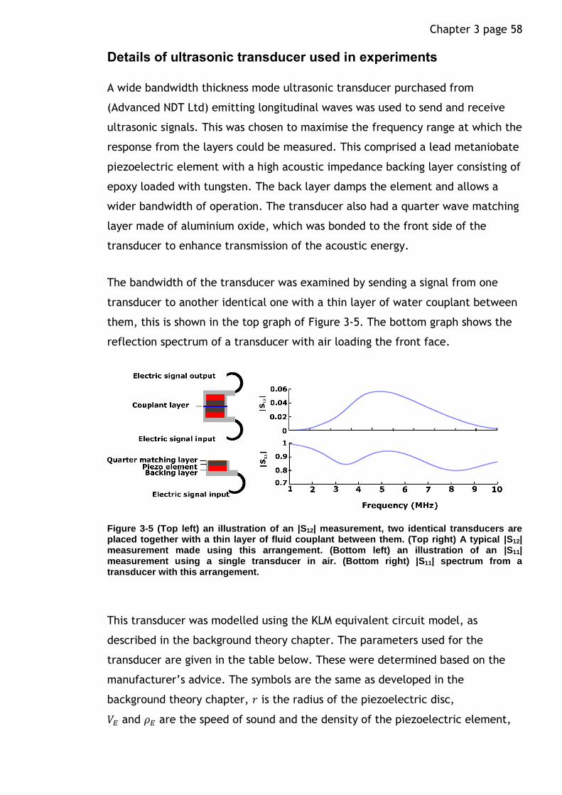
Chapter 3 page 58

Details of ultrasonic transducer used in experiments

A wide bandwidth thickness mode ultrasonic transducer purchased from

(Advanced NDT Ltd) emitting longitudinal waves was used to send and receive

ultrasonic signals. This was chosen to maximise the frequency range at which the

response from the layers could be measured. This comprised a lead metaniobate

piezoelectric element with a high acoustic impedance backing layer consisting of

epoxy loaded with tungsten. The back layer damps the element and allows a

wider bandwidth of operation. The transducer also had a quarter wave matching

layer made of aluminium oxide, which was bonded to the front side of the

transducer to enhance transmission of the acoustic energy.

The bandwidth of the transducer was examined by sending a signal from one

transducer to another identical one with a thin layer of water couplant between

them, this is shown in the top graph of Figure 3-5. The bottom graph shows the

reflection spectrum of a transducer with air loading the front face.

Figure 3-5 (Top left) an illustration of an |S12| measurement, two identical transducers are placed together with a thin layer of fluid couplant between them. (Top right) A typical |S12| measurement made using this arrangement. (Bottom left) an illustration of an |S11| measurement using a single transducer in air. (Bottom right) |S11| spectrum from a transducer with this arrangement.

This transducer was modelled using the KLM equivalent circuit model, as

described in the background theory chapter. The parameters used for the

transducer are given in the table below. These were determined based on the

manufacturer’s advice. The symbols are the same as developed in the

background theory chapter, 𝑟 is the radius of the piezoelectric disc,

𝑉𝐸 and 𝜌𝐸 are the speed of sound and the density of the piezoelectric element,

Chapter 3 page 59

𝑘𝑇 is the piezo-electric coupling factor, 휀𝑅𝑆 is the clamped relative permittivity,

𝑉𝑚 and 𝜌𝑚 are the speed of sound and density in the matching layer and 𝑄𝐸 is a

measure of the mechanical loss in the transducer, 𝑄𝐸 = 4.343 (2𝜋𝑓

𝑉𝐸𝛼𝐸).

Property

r 10 mm

𝒅𝑬 2.4 x10-4 m

𝜺𝑹𝑺 2.655x10-9 Fm-1

𝒌𝑻 0.35

𝑽𝑬 3050 ms-1

𝝆𝑬 6200 kgm-3

𝑸𝑴 15

𝑪𝒎 2914 ms-1

𝝆𝒎 3710 kgm-3

Table 1 Parameter values used to model the ultrasonic transducers in the experiments. These were set using guidance from the manufacturer apart from the properties of aluminium oxide which were taken from (Wachtman & LAM 1959)

Details of experiments with acoustic layered systems

The acoustic reflecting layers were fabricated using spacers to hold a number of

silicon wafers or glass coverslips apart with magnets applied top and bottom to

keep the structure together. UV curable glue was then applied carefully to the

sides and UV light was applied to cure the glue. The spacers were then removed,

this is illustrated in Figure 3-6. The thickness of the spacers and layers was

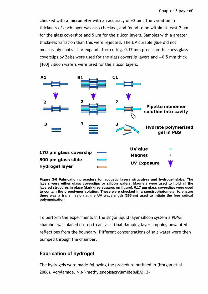
Chapter 3 page 60 checked with a micrometer with an accuracy of ±2 µm. The variation in

thickness of each layer was also checked, and found to be within at least 2 µm

for the glass coverslips and 5 µm for the silicon layers. Samples with a greater

thickness variation than this were rejected. The UV curable glue did not

measurably contract or expand after curing. 0.17 mm precision thickness glass

coverslips by Zeiss were used for the glass coverslip layers and ~0.5 mm thick

[100] Silicon wafers were used for the silicon layers.

Figure 3-6 Fabrication procedure for acoustic layers strucutres and hydrogel slabs. The layers were either glass coverslips or silicon wafers. Magnets were used to hold all the layered strucures in place (dark grey squares on figure). 0.17 µm glass coverslips were used to contain the prepolymer solution. These were checked in a spectrophotometer to ensure there was a transmission at the UV wavelength (365nm) used to intiate the free radical polymerisation.

To perform the experiments in the single liquid layer silicon system a PDMS

chamber was placed on-top to act as a final damping layer stopping unwanted

reflections from the boundary. Different concentrations of salt water were then

pumped through the chamber.

Fabrication of hydrogel

The hydrogels were made following the procedure outlined in (Horgan et al.

2006). Acrylamide, N,N’-methylenebisacrylamide(MBA), 3-

Chapter 3 page 61 Acrylamidophenylboronic acid(3-APB) and 3-

acrylamidopropyltrimethylammonium chloride (ATMA) were mixed in molar

percentages of 73/3/12/12 respectively. 2,2-demthoxy-2-phenylacetophenone

(DMPA) was then dissolved in dimethyl sulfoxide (DMSO) at a concentration of 2%

(w/v). The monomer mixture was added to the solution so that there was a ratio

of 1:2.21 (w/v) of monomers to solvent. The solutions were then stored in sealed

containers away from light. To create the hydrogels, two glass slides treated

with trichloro (1H,1H,2H,2H-perfluorooctyl) silane were placed apart by a

spacer, the solution was then pipetted into the gap and the whole structure was

exposed to UV radiation for 30 minutes using a (UV KUB 1 KLOE). This uses LEDs

to emit cold UV radiation at 365nm wavelength. After polymerisation the glass

slides were removed and the polymerised hydrogel slab was hydrated and

washed several times to remove the DMSO before being immersed in PBS solution

at PH 7.4 and left for 24 hours to equilibrate.

The DMPA acts as the initiator of a free radical chain polymerisation of the

acrylamide, 3APB, MBA and ATMA monomers. The reaction is initiated by

exposing the solution to UV light which leads to fragmentation of the DMPA into

radicals which are able to react with a monomer by breaking open its double

carbon bond. The unpaired electron is transferred to the end of the two-

molecule chain which is in turn is able to break open and bond with another

monomer, with the unpaired electron again transferred to the end of the chain.

Over a number of steps a long chain of monomers is formed and continues to

grow until the reaction is terminated by reaction with another radical for

example the end of another growing chain (Ravve 2000).

Optical measurements of hydrogel thickness

The hydrogel samples were very soft and consequently their thickness could not

be determined using a micrometer. Instead thickness measurements of the

hydrogels were carried out using a microscope to image the hydrogel samples

from the side. A spirit level was used to ensure the hydrogel slabs and the

microscope camera were aligned correctly. The sample thickness was then

determined by converting the measured pixel thickness of the image. A

calibration was performed before hand using solid flat materials such as glass

and silicon that could be also measured with the micrometer. Figure 3-7 shows a

Chapter 3 page 62 graph of the calibration curve created using different thickness of substrate. The

width of the errorbars is the standard deviation of five repeat measurements.

Figure 3-7 Calibration curve for microscope thickness measurements. The gradient was found to be 0.5787 µm pixel-1 using a least square fit of the data. The mean absolute error

was 5.8 𝛍𝐦.

The x axis is the thickness measured using a micrometer and the y axis shows the

pixel thickness from the microscope image. This was measured using imagej. A

least squares fit found the micro meter to pixel ratio as 0.58 µm pixel-1.

Measurement accuracy was estimated by finding the mean absolute error which

was 5.8 µm.

3.3 Details of COMSOL simulations

COMSOL 3.5 was used to create three separate simulations in this thesis.

In the SAW streaming investigation COMSOL was used to create two separate

simulations. Firstly it was used to simulate the sound field that a leaky SAW

radiated into a fluid. This was used as a verification step, to check that an

analytical expression of the sound field correctly matched this simulation. In a

separate simulation the streaming in a microfluidic volume due to a SAW was

Chapter 3 page 63 also modelled using COMSOL. This simulation solved the Navier Stokes equation,

where an expression for the body force on the fluid was used to describe the

influence of the SAW. The body force was derived from the analytical expression

for the sound field using Nyborg’s streaming equations, as described in chapter

four.

COMSOL was also used to model the acoustic reflection spectrum from a layered

structure at an angle to the acoustic beam, that was of interest in the acoustic

sensor part of the thesis. The details of these three simulations are presented

below, but firstly a brief introduction to COMSOL and the FEM method is given.

COMSOL Multiphysics 3.5 (Comsol Inc n.d.) is a software package that can be

used to solve a wide variety of different physics based problems. After the user

specifies the geometry, material properties and the physical equations governing

the problem, COMSOL uses the finite element method to solve the equations

over the whole geometry specified by the user. COMSOL has a large of set of

predefined equations already built in that can be used to simulate common

physical problems such as acoustic waves and fluid dynamics among others. A

particular advantage of COMSOL is that different physical equations can be

coupled together, allowing simulation of more complex systems.

COMOSL uses the finite element method to find a solution to the partial

differential equations governing the physics of the system. This involves

discretizing the overall geometry into small regions where the variables of

interest can be estimated with simpler algebraic equations. The problem is

solved by finding a solution that satisfies all these equations to within a given

error tolerance. The more regions, or elements a problem has the longer it takes

to solve, however the more accurate the solution becomes.

Streaming from Leaky SAWs – sound field in fluid domain

Fluid flow caused by leaky SAW vibrations was simulated in 3 parts. The first

part was to find an expression for the sound field in the fluid. A simple

improvement to the equations in the literature was introduced to properly

model the attenuation of the sound beam, this is described in detail in chapter

four. To verify this and also show the significance a simulation of the sound field

Chapter 3 page 64 in the fluid was written in COMSOL. The final step was a simulation of the fluid

flow due to the sound field which was done using COMSOL by solving the

incompressible Navier Stokes equation.

The sound field in a fluid due to a leaky SAW propagating along one of the

boundaries was simulated using the pressure acoustic application mode in 2D.

Mesh density, geometry and boundary conditions

The 2D geometry was set as a rectangular shape in the sagittal plane of the

leaky SAW beam, with the physical properties set to water, and the Leaky SAW

vibration propagating along the bottom boundary. This was incorporated by

choosing a normal acceleration boundary condition along the boundary, (i.e. the

acceleration component perpendicular to the boundary) the normal acceleration

of a leaky SAW wave propagating along the surface is,

𝛼𝑛 = 𝑒(−𝑘𝑌−𝛼𝑠𝑎𝑤𝑌) 3-3

Where 𝑘𝑌 =2𝜋𝑓

𝑉𝑠𝑎𝑤 and 𝛼𝑠𝑎𝑤 is the attenuation coefficient of the leaky SAW beam.

It is not necessary to include the component of the leaky SAW parallel to the

fluid domain as this does not have a large effect on the sound field in the fluid

outside of the viscous boundary layer, which for the MHz frequencies used in

SAW devices is just a few nanometers thick. (Vanneste & Buhler 2010).

The other boundary conditions were set to impedance match the fluid layer

using the impedance boundary condition. This was found to be effective for

eliminating reflections back into the fluid domain.

The mesh density was set so that the wavelength at each frequency was at least

10 times bigger than the minimum element size.

Physical properties and solution settings

The fluid domain was set as water at 20 ℃. A general damping factor was added

to the water to properly simulate the attenuation of the sound beam as it

Chapter 3 page 65 propagates through the fluid domain (see background theory chapter). The

solver parameters were set to time-harmonic analysis.

Streaming from Leaky SAWs – fluid flow simulation

COMSOL was also used to simulate fluid streaming induced by leaky SAWs. The

compressible Navier Stokes equation application mode in 3D was selected to do

this.

Mesh density, geometry and boundary conditions

For comparison with experiment the geometry was set to the same dimensions

as the PDMS chamber which was 400 by 400 by 145 µm. The height of the

chamber was determined using a dektak on the finished PDMS su-8 mold. No-slip

boundary conditions were imposed on all of the walls.

An appropriate mesh density was set by systematically increasing the mesh

density from very coarse to very fine and observing the differences in the

solution. The mesh density was then chosen by a trade-off between accuracy

and solution time. The maximum element size was set as 20 µm with all the

other values kept at the default settings.

Body force and solution settings

An analytical expression for the body force acting on the fluid was used to

describe the action of the sound-field on the fluid flow (see chapter four). The

analysis type was set to stationary and a parametric solver was used to vary the

frequency in the body force expression. The linear system solver was set to

BiCGSTab, the preconditioner was set to incomplete LU. The drop tolerance was

set to 5x10-4.

Acoustic waves in elastic and fluid materials

COMSOL (Comsol Inc n.d.) can be used to model pressure fields and mechanical

deformations in different materials such as elastic solids and pure liquids. Two

different application modes are required to model acoustic waves in a system

containing elastic solid and fluid mediums.

Chapter 3 page 66 The pressure acoustics application mode solves the classical wave equation for a

fluid, (see background theory chapter) i.e. it is assuming the material medium

acts like a Newtonian fluid. The stress-strain application mode solves the

equation of motion for an elastic solid. Different application modes can be used

depending on the number of dimensions required. The plane strain application

for example, models the stresses and strains over a two dimensional domain,

assuming that are no out of plain strain components. Both of these application

modes are of-course operating under the assumptions of the underlying

equations, i.e. a continuous material medium, based on either Hook’s law or

Newton’s viscosity law.

A further important consideration comes from the choice of the element size,

which has to be small enough to properly resolve the wavelengths in the domain.

A rule of thumb is to have about 10-12 degrees of freedom per wavelength

(Comsol Inc n.d.). This results in rather dense meshes which can take a long time

to solve for large problems.

COMSOL simulation of transmission properties in layered media consisting of both elastic and fluid mediums.

The purpose of this simulation was to investigate the transmission and reflection

of an angled sound beam on the acoustic layered structure that is investigated as

a potential acoustic sensing platform in chapter 6. A series of parallel sided

layers are stacked onto of each other, alternating between solid and liquid

layers.

The simulation was built following the method described in the COMSOL

mulitphysics database titled “Acoustic transmission loss through periodic elastic

strucutres”. In this method periodic boundary conditions are used to reduce the

geometric size of the domains and speed up computation time. This effectively

makes the simulation that of an acoustic stack that is infinitely wide in the

direction parallel with the layer boundaries.

Mesh density, geometry and boundary conditions

When modelling acoustic wave interactions between liquid and solid media,

different equations must be used in each domain. These are coupled by

Chapter 3 page 67 boundary conditions at the interface. The pressure acoustics application module

was used for the fluid domain and the plain strain application mode was used for

the elastic solid domain.

The interaction between the fluid and solid domain were simulated by

expressing the load of the fluid on the solid as the normal component of

pressure in the fluid. The effect of the solid domain on the fluid was expressed

using the normal acceleration boundary condition. Perfect matching layers were

used at the top and bottom of the simulation to damp any reflections from the

edges of the simulation. Periodic boundary conditions were imposed on the

sides. The minimum element size of the mesh in both domains was set to at

least one tenth of the wavelength in the fluid domain.

Physical properties and solution settings

The physical properties of the fluid domain was set to water at 20 ℃ and the

solid domain was set to that of an isotropic elastic solid having a Young’s

modulus of 169.98 GPa and a density of 2330 kgm-3. This is the speed of sound of

silicon in the [100] direction, which was the material choice used in the 1D

scattering matrices of the investigation, however an isotropic elastic solid was

chosen here to keep the analysis simple.

The simulation was solved using the time harmonic and frequency domain solvers

using a parametric sweep of the frequency or incidence angle of the ultrasonic

beam. The transmission and reflection coefficients were calculated by solving

for the absolute pressure at the start and end boundaries for the incident and

outgoing waves and dividing by the width of the boundary.

page 68

Chapter 4 Development of SAW streaming simulation

This chapter discusses the development of a simulation that can accurately

predict the streaming in an arbitrary microfluidic chamber due to a leaky SAW

wave of arbitrary frequency. The workflow is shown in Figure 4-1, it involves a

two-step approach. First an expression for the sound field radiated into the fluid

by the SAW is developed. Then the body force on the fluid is derived using

equation 2-47 which links the body force with the sound field as described in the

background theory chapter (Nyborg 1958). The final body force expression is

then used in the 3D COMSOL flow simulation which solves the incompressible

Navier-Stokes equation.

It is tempting to try to simulate the whole system (sound field and streaming) in

one seamless coupled physics simulation, however the simulation of the sound

field in 3D at the very high frequencies of interest here comes with a large

computation cost, luckily the flow simulation is much faster to run. This is why

instead only the fluid flow is simulated using FEM simulation, with influence of

the acoustic field included by the expression for the body force. This semi-

numerical method for modelling SAW streaming was also used in the work of

(Alghane 2013).

In order to check the sound field expression a less computationally expensive 2D

simulation of the sound field was used to compare and further develop the

expressions used in the flow simulation. Many other 2D simulations of the sound

field radiated into the fluid by a SAW have been performed using various

different numerical methods with results that agree qualitatively with those

found here, for example (Vanneste & Buhler 2010). The novelty here was to use

this as a gold standard by which to judge the analytical expression. The

analytical expression used here was very similar to that found in (Frommelt et

al. 2008) and (Collins et al. 2016) however the 2-D simulations made clear that a

small improvement could be made by including the anechoic corner (as coined

by (Destgeer et al. 2015)).

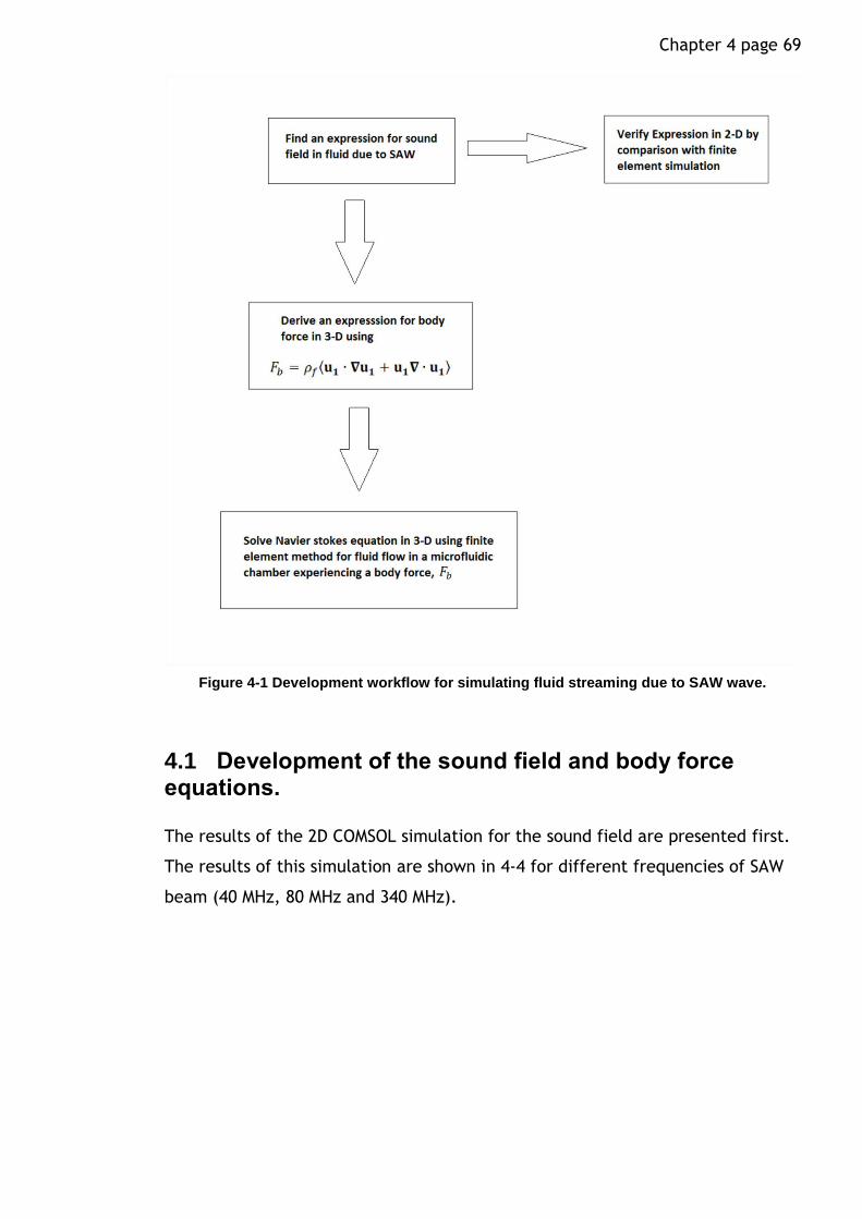
Chapter 4 page 69

Figure 4-1 Development workflow for simulating fluid streaming due to SAW wave.

4.1 Development of the sound field and body force equations.

The results of the 2D COMSOL simulation for the sound field are presented first.

The results of this simulation are shown in 4-4 for different frequencies of SAW

beam (40 MHz, 80 MHz and 340 MHz).

Chapter 4 page 70

Figure 4-2 COMSOL simulation results of the sound field radiated into a fluid by a leaky SAW propagation along the bottom boundary from left to right. (Top left) Illustration of the geometry, the SAW propagates along the bottom boundary starting at the origin, the fluid domain is rectangular and starts at the origin extending for Z >0 and Y >0. (Top right) Pressure field generated at 40 MHz (Bottom left) Pressure field generated at 80 MHz. (Bottom right) Pressure field generated at 340 MHz.

The top left illustration shows the SAW vibration in relation to the fluid, where

the SAW propagates along the bottom boundary from left to right and attenuates

according to 𝛼𝑠𝑎𝑤. The colour graphs show the pressure field generated in the

fluid, this takes the form of an angled plane wave, albeit with some additional

interference patterns. The angle of propagation is the Rayleigh angle,

determined by 𝜃𝑅 = 𝑠𝑖𝑛−1 (𝑉𝑓

𝑉𝑆𝐴𝑊). As the frequency increases from 40 to 340 MHz

the attenuation length of the SAW beam decreases proportionally with the

frequency, this consequently means that the sound field does not penetrate so

far in the fluid along the Y direction. The beam penetrates much further into the

depth of the fluid, where the attenuation length is governed by the viscous

damping of the fluid, which for frequencies below 500 MHz is comparatively

longer. The frequency scaling of the sound field is governed by these two

attenuation coefficients however they scale with frequency differently. The

attenuation of a leaky SAW and a compression wave in a viscous fluid can be

written as,

Chapter 4 page 71

𝛼𝑠𝑎𝑤 =

𝜌𝑓𝑉𝑓𝜌𝑠𝑉𝑆𝐴𝑊𝜆𝑆𝐴𝑊

4-1

𝛼𝑓 =

𝑏𝜔2

2𝜌𝑓𝑉𝑓3

4-2

Where 𝛼𝑓 is the attenuation of a compression wave propagating through water

(Michael B. Dentry et al. 2014). Where 𝑏 = (4

3𝜇 + 𝜇′) and 𝜇′ is the bulk viscosity

of the fluid and 𝜇 is the shear viscosity, 𝛼𝑠𝑎𝑤 is the well known attenuation

length for a fluid loaded leaky SAW,(Cheeke & Morisseau 1982). Figure 4-1

compares the attenuation length of 𝛼𝑠𝑎𝑤 and 𝛼𝑓 as a function of frequency. The

attenuation length of the leaky SAW varies with 1

𝑓 and is significantly shorter

than the compression wave, which varies as 1

𝑓2 .

Figure 4-3 Comparison of attenuation lengths of a water loaded leaky SAW (red line) and a compression wave (blue line) propagating through water as a function of frequency. The leaky SAW attenuation length is calculated according to equation 4-1. The attenuation length for a compression wave is calculated from equation 4-2.

Chapter 4 page 72 An expression for the radiated sound field must therefore be in the form of an

angled compression wave that attenuates due to viscous damping of the fluid

and also the attenuation of the SAW. A description for this has been attempted

several times in the literature with varying degrees of success, the next section

discusses the different approaches that have been used and further adds to the

accuracy of the expression.

Most previous workers start with an expression for a compression wave

propagating at the Rayleigh angle in the Y-Z plane. This can be described using,

𝑢𝑌 = 𝐴𝑦𝑒

𝑖𝜔𝑡𝑒−𝑖𝑘𝑌𝑌𝑒−𝑖𝑘𝑍𝑍 4-3

𝑢𝑍 = 𝐴𝑧𝑒𝑖𝜔𝑡𝑒−𝑖𝑘𝑌𝑌𝑒−𝑖𝑘𝑍𝑍

4-4

Where 𝑢𝑌 and 𝑢𝑍 are the Y and Z components of the fluid particle velocity, 𝐴𝑌

and 𝐴𝑍 are amplitude factors and 𝑘𝑌 and 𝑘𝑍 are the complex wavenumbers in

the Y and Z direction. The Z axis is set as normal to the SAW beam propagation

(i.e. the depth into the fluid) and the Y axis is parallel with the propagation

direction. The real parts of the wavenumbers describe the wavelength and

propagation direction of the wave, while the imaginary parts describe the

attenuation of the sound field.

To correctly describe the SAW radiated sound field both the viscous damping of

the fluid and attenuation of the SAW beam must be included in how the

wavenumbers in equations 4-3 and 4-4 are written. A simulation for SAW

streaming in micro-droplets was developed by (Alghane 2013) in which the body

force was derived by first considering the sound field in the drop. Unfortunately,

as has been pointed by other authors this description did not include the

frequency dependant viscous damping of the fluid but only the damping

coefficient of the SAW (Collins et al. 2016; Michael B. Dentry et al. 2014). This

turns out to be very important for accurately describing the scaling of SAW

streaming in restricted fluid volumes.

A more accurate method for describing the sound field using a ray tracing

approximation has also be tried (Frommelt et al. 2008). Using this method each

point along the vibrating surface is described as emitting a beam into the fluid

Chapter 4 page 73 which propagates at the Rayleigh angle and attenuates according to the viscous

damping of the fluid. The initial amplitude of each beam at the surface is

determined by the attenuation of the SAW to get to that point. This is illustrated

in Figure 4-4, to determine the attenuation of the sound field at a point P in the

fluid, a line of distance D is drawn from the point back to the surface at the

Rayleigh angle, then another line of distance S is drawn back to the meeting

point of the SAW and fluid. The total attenuation from the initial acoustic

energy is then 𝑒−𝑆𝛼𝑠𝑎𝑤𝑒−𝐷𝛼𝑓.

Figure 4-4 Illustration of the trigonometric reasoning used to derive the sound field in the fluid. The SAW travels from left to right, meeting the fluid at the origin where it attenuates as

𝜶𝒔𝒂𝒘

Chapter 4 page 74 Following trigonometric arguments this sound field can described in terms of the

Y and Z direction as,

𝑢𝑌 = 𝜔𝐴tan(θ)𝑒𝑖(𝜔𝑡−𝑘𝑌𝑌−𝑘𝑍𝑍)𝑒(−|𝑌−𝑍tan(𝜃𝑅)|𝛼𝑠𝑎𝑤)−𝑍𝑐𝑜𝑠

−1(𝜃𝑅)𝛼𝑓

4-5

𝑢𝑍 = 𝜔𝐴𝑒𝑖(𝜔𝑡−𝑘𝑌𝑌−𝑘𝑍𝑍)𝑒(−|𝑌−𝑍tan(𝜃𝑅)|𝛼𝑠𝑎𝑤)−𝑍cos

−1(𝜃𝑅)𝛼𝑓

4-6

Where 𝑘𝑌 = |𝐤|sin(𝜃𝑅) and 𝑘𝑍 = |𝐤|cos(𝜃𝑅) are the real parts of the wave

number in the Y and Z directions with |𝐤| =2𝜋𝑓

𝑉𝑓 and 𝜃𝑅 = sin−1(

𝑣𝑓

𝑣𝑆𝐴𝑊) is the

Rayleigh angle. The amplitude is rewritten arguing that it is reasonable to write,

𝐴𝑍 = 𝐴𝑌tan (𝜃𝑅), where 𝐴𝑌 is initial displacement amplitude of the SAW. 𝐴𝑌 can

then be substituted into equation 4-5, and the subscript dropped.

This equation is written slightly differently to (Frommelt et al. 2008) in order to

make it compatible with the COMSOL interface, a very similar equation can also

be found in (Collins et al. 2016)). These equations should correctly account for

the attenuation of the sound beam due to both the attenuation of the leaky SAW

and the attenuation with propagation into the fluid. At the fluid substrate

interface the fluid particle velocity is equal to the leaky SAW velocity, and

therefore attenuates with 𝛼𝑠, however as the wave propagates out from the

substrate it will attenuate with 𝛼𝑓. The attenuation factor at (𝑍 = 0) reduces to

attenuation of the SAW beam.

A comparison of equation 4-5 with the COMSOL (Comsol Inc n.d.) simulation

results for a 342 MHz SAW wave with an initial amplitude of 87 picometers is

shown in Figure 4-5. The left hand figure is 𝑢𝑍 described by equation 4-5. The

right hand figure is again the COMSOL(Comsol Inc n.d.) simulation for a 342 MHz

SAW wave. The colour scale is the same for both figures so that a comparison

can be made.

Chapter 4 page 75

Figure 4-5 Comparison of Z component of velocity field between (right) the COMSOL(Comsol

Inc n.d.) simulation and (left) Equation 4-5. The Colour scale on the right is for both figures. The SAW propagates along the bottom (Y) axis.

To further clarify the quantitative differences a cross section at Z=100 μm of

the Y component of the velocity field is shown in Figure 4-6.

Figure 4-6 Cross section of uY at Z= 100 μm. The blue line shows the predictions from

equation 4-5 and the red lines shows the simulation results.

From Figure 4-5 and Figure 4-6 it can be seen that equations 4-5 and 4-6 give an

accurate account of the sound field attenuating correctly along the length of the

beam, however the top left hand corner of the chamber where there is no

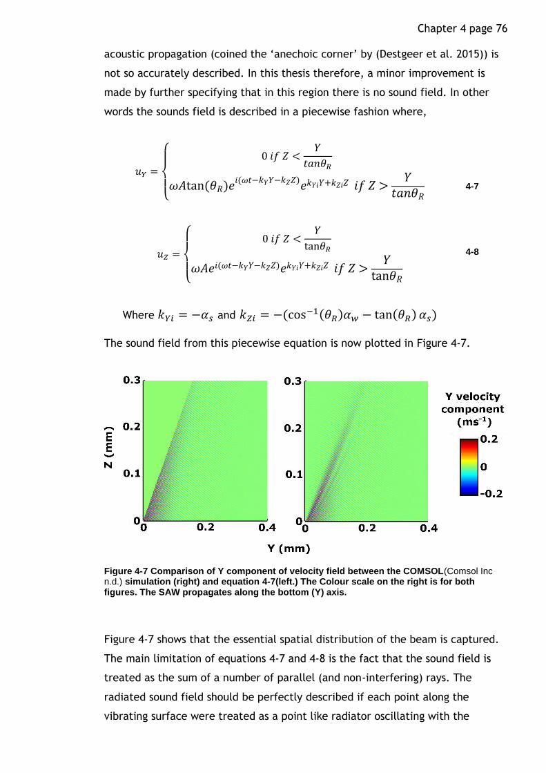
Chapter 4 page 76 acoustic propagation (coined the ‘anechoic corner’ by (Destgeer et al. 2015)) is

not so accurately described. In this thesis therefore, a minor improvement is

made by further specifying that in this region there is no sound field. In other

words the sounds field is described in a piecewise fashion where,

𝑢𝑌 =

{

0 𝑖𝑓 𝑍 <

𝑌

𝑡𝑎𝑛𝜃𝑅

𝜔𝐴tan (𝜃𝑅)𝑒𝑖(𝜔𝑡−𝑘𝑌𝑌−𝑘𝑍𝑍)𝑒𝑘𝑌𝑖𝑌+𝑘𝑍𝑖𝑍 𝑖𝑓 𝑍 >

𝑌𝑡𝑎𝑛𝜃𝑅

4-7

𝑢𝑍 =

{

0 𝑖𝑓 𝑍 <

𝑌

tan𝜃𝑅

𝜔𝐴𝑒𝑖(𝜔𝑡−𝑘𝑌𝑌−𝑘𝑍𝑍)𝑒𝑘𝑌𝑖𝑌+𝑘𝑍𝑖𝑍 𝑖𝑓 𝑍 >𝑌

tan𝜃𝑅

Where 𝑘𝑌𝑖 = −𝛼𝑠 and 𝑘𝑍𝑖 = −(cos−1(𝜃𝑅)𝛼𝑤 − tan(𝜃𝑅) 𝛼𝑠)

4-8

The sound field from this piecewise equation is now plotted in Figure 4-7.

Figure 4-7 Comparison of Y component of velocity field between the COMSOL(Comsol Inc n.d.) simulation (right) and equation 4-7(left.) The Colour scale on the right is for both figures. The SAW propagates along the bottom (Y) axis.

Figure 4-7 shows that the essential spatial distribution of the beam is captured.

The main limitation of equations 4-7 and 4-8 is the fact that the sound field is

treated as the sum of a number of parallel (and non-interfering) rays. The

radiated sound field should be perfectly described if each point along the

vibrating surface were treated as a point like radiator oscillating with the

Chapter 4 page 77 amplitude of the SAW at that point. The sum of the fields radiated by each point

would then be the field as shown by the numerical simulation, and should also

describe the interference patterns see in the numerical simulation. Such a

description would be a near impossible task to perform however. So equations

4-7 and 4-8 are probably about as good a description of the sound field as is

possible to reach. They have not been derived from the underlying equations of

motion but rather they are based on intuitive reasoning about the attenuation of

the beam.

With the sound field described by equations 4-7 and 4-8 the body force on the

fluid can be calculated using the streaming equations described in chapter two.

These are,

𝐹𝑌 = 𝜌𝑓(tan(𝜃𝑟)𝑘𝑌𝑖 + 𝑘𝑍𝑖)𝐴2𝜔2tan(θR)𝑒

2(𝑘𝑌𝑖+𝑘𝑍𝑖)

𝐹𝑧 = 𝜌𝑓(tan(𝜃𝑟)𝑘𝑌𝑖 + 𝑘𝑍𝑖)𝐴2𝜔2𝑒2(𝑘𝑌𝑖+𝑘𝑍𝑖)

4-9

4.2 Vibrometer measurements

So far the body force description has been confined to two dimensions (defined

as Y and Z here). In order to properly describe the variation in the amplitude of

the SAW beam in the third dimension 𝐴 in equation 4-9 can be rewritten as a

function of the X direction. This was chosen by best fitting a curve to the SAW

beam amplitudes measured by the vibrometer.

Figure 4-8 shows an illustration of the PDMS microchambers used in the

streaming experiments. The SAW beam propagates outwards from the IDT until it

encounters the PDMS slab, where it is either damped by the PDMS or allowed to

propagate through the dry channel (beam tunnel). A vibrometer scan of an 87

MHz SAW propagating across the chamber is shown on the left. The effect of the

beam tunnel is clearly evident, with the SAW beam amplitude much greater on

the right hand side of the chamber.

Chapter 4 page 78

X

Y

Amplitude of SAW beam in PDMS chamber

The vibrometer measurements presented in the following section were all taken

after the corresponding micro PIV measurements with the PDMS channel

structure remaining in position on the surface. The chamber was flushed with

clean DI water to remove the florescent beads used in the PIV measurement and

then allowed to dry. The SAW velocity amplitudes were measured along the

position where the SAW beam first makes contact with the fluid. This is the

bottom right hand corner of the PDMS chamber in Figure 4-9.

Figure 4-9 shows some examples of SAW waves in the chamber for 342 and 87

MHz beam, with an illustration of the chamber structure superimposed on-top

for clarity. The colour scale indicates displacement magnitude.

Figure 4-8 Right shows an illustration of the PDMS chamber design used in the experiments in this chapter. A SAW beam is generated at an IDT and then propagates along the substrate surface. At the boundary with the PDMS it is spatially filtered by the Beam tunnel over a distance of 15mm. It then travels across the PDMS chamber causing fluid streaming. The chamber was 0.4 by 0.4 mm in the X-Y plane and 0.145 mm in the Z plane (pointing normal to the page). Left shows a vibrometer scan of the SAW beam in the chamber superimposed onto a sketch of the chamber with the inlet and outlet visible.

Chapter 4 page 79

Figure 4-9 Vibrometer scans of the leaky SAW waves inside the dry PDMS chambers. An illustration of the chambers has been superimposed over the top so the positioning of the SAW beam relative to the microchamber is clear. The scan shows an instantaneous value of the displacement magnitude.

This shows that the beam is confined to the right hand side of the chamber in

both cases. The 87 MHz beam exhibits more wave spreading as it propagates

through the micro-chamber.

An example cross section of the SAW beam just as it enters the micro-chamber

for 43 and 342 MHz is given in Figure 4-10 and Figure 4-11 respectively. The axis

labelled X follows from the coordinate system used in the previous section,

where the origin is placed at the bottom left hand corner of the chamber. The

legends show the electrical power inputs to the IDT. The SAW velocity axis shows

the SAW particle velocity for each X position. Each data point on the figure is

the average of 3 measurements and the error bars are the standard deviation of

these measurements.

One way of putting this information into the simulation is to fit the vibrometer

data to an analytical function. Equation 4-9 can then be modified by replacing

Chapter 4 page 80 the amplitude constant with something that varies as a function of the x axis.

For the 87 and 43 MHz beams a Gaussian function was fitted i.e.

𝐹 = 𝐴𝑒

−(𝑥−𝑏𝐶)2

4-10

Where a, b and c are chosen to fit the data. The profiles fit this function with a

root mean square error of at least less than 10% of the maximum amplitude of

the Gaussian profile, which is close to the typical standard deviation for each

data point.

Figure 4-10 Beam profile in the chamber for 43 MHz SAW wave at different input powers.

The 342 MHz SAW beam used in the PIV measurements is less well described with

a single Gaussian function and was instead described using a double Gaussian

function. An example is given in Figure 4-12.

Chapter 4 page 81

Figure 4-11 Beam profile in Chamber for the 342 MHz SAW wave at different input powers.

Figure 4-12 Example of Gaussian fit against measured beam profile at 1 W for the 342 MHz SAW beam

Amplitude of SAW beam in the tunnel

The SAW beam was also measured in the tunnel directly before entering the

chamber. By comparing the amplitude of the SAW beam in the tunnel and in the

chamber the attenuation of the SAW beam as it propagates through the PDMS

wall separating these two regions can be estimated. If the SAW leaks energy into

the PDMS in the same manner as a fluid, one might expect it to attenuate as

Chapter 4 page 82

𝛼𝑝𝑑𝑚𝑠 =𝜌𝑝𝑑𝑚𝑠𝑐𝑝𝑑𝑚𝑠𝜌𝑠𝑉𝑅𝜆𝑆𝐴𝑊

4-11

Where 𝜌𝑝𝑑𝑚𝑠 and 𝑐𝑝𝑑𝑚𝑠 are the density and the speed of sound in 𝑝𝑑𝑚𝑠

respectively. The attenuation coefficient of the PDMS can then be calculated

from the measurements by using,

𝛼 = −1

𝑌𝑙𝑛 (

𝐴(𝑦)

𝐴(0)) 4-12

In this equation 𝐴(0) is the initial amplitude of the SAW beam and 𝑌 is the

propagation distance. The thickness of the PDMS wall in this experiment was 100

μm. Since the beam is Gaussian shaped each point is compared with its

counterpart on the other side of the wall, with the overall measured attenuation

coefficient being the average of all these points.

𝛼𝑝𝑑𝑚𝑠 and the measured 𝛼 are plotted in Figure 4-13 as a function of frequency.

The width of the error bars is the standard deviation of the attenuation

measured for all the data points in the SAW beam cross section.

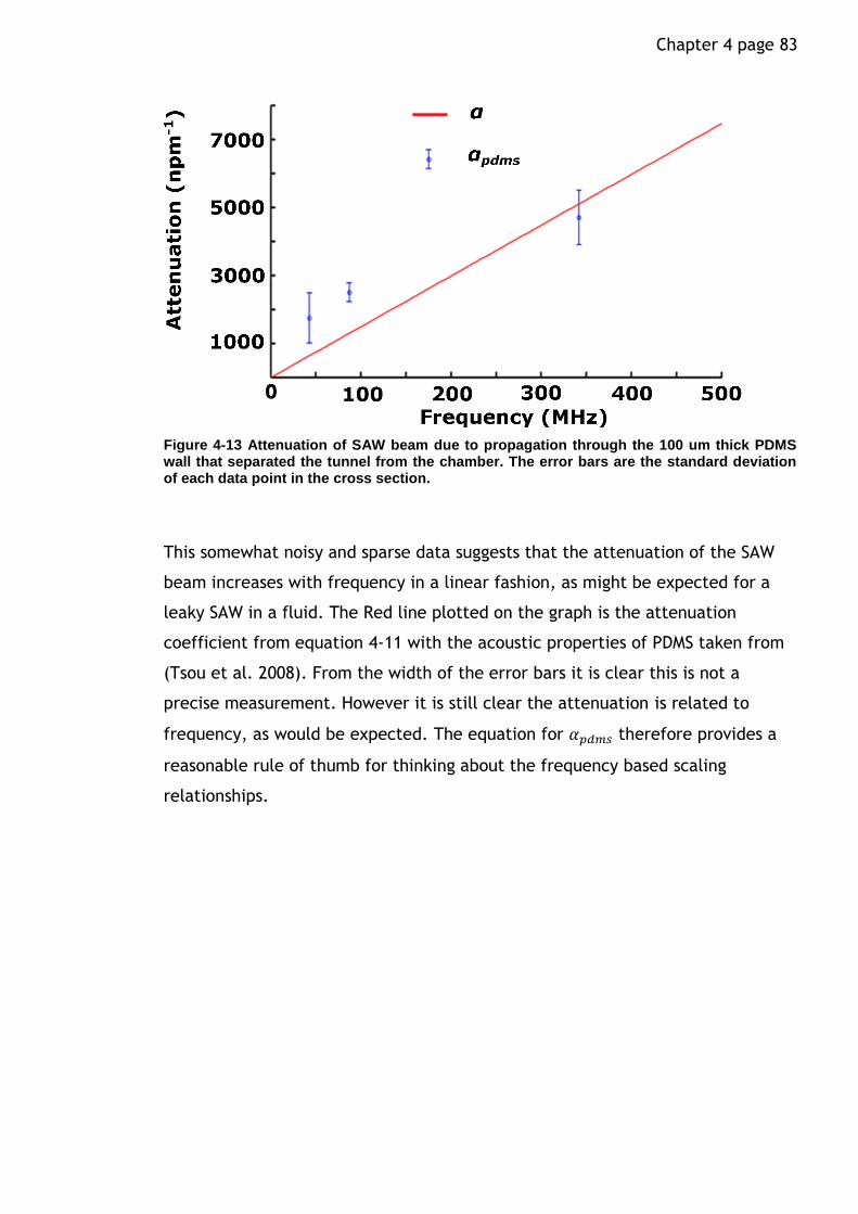
Chapter 4 page 83

Figure 4-13 Attenuation of SAW beam due to propagation through the 100 um thick PDMS wall that separated the tunnel from the chamber. The error bars are the standard deviation of each data point in the cross section.

This somewhat noisy and sparse data suggests that the attenuation of the SAW

beam increases with frequency in a linear fashion, as might be expected for a

leaky SAW in a fluid. The Red line plotted on the graph is the attenuation

coefficient from equation 4-11 with the acoustic properties of PDMS taken from

(Tsou et al. 2008). From the width of the error bars it is clear this is not a

precise measurement. However it is still clear the attenuation is related to

frequency, as would be expected. The equation for 𝛼𝑝𝑑𝑚𝑠 therefore provides a

reasonable rule of thumb for thinking about the frequency based scaling

relationships.

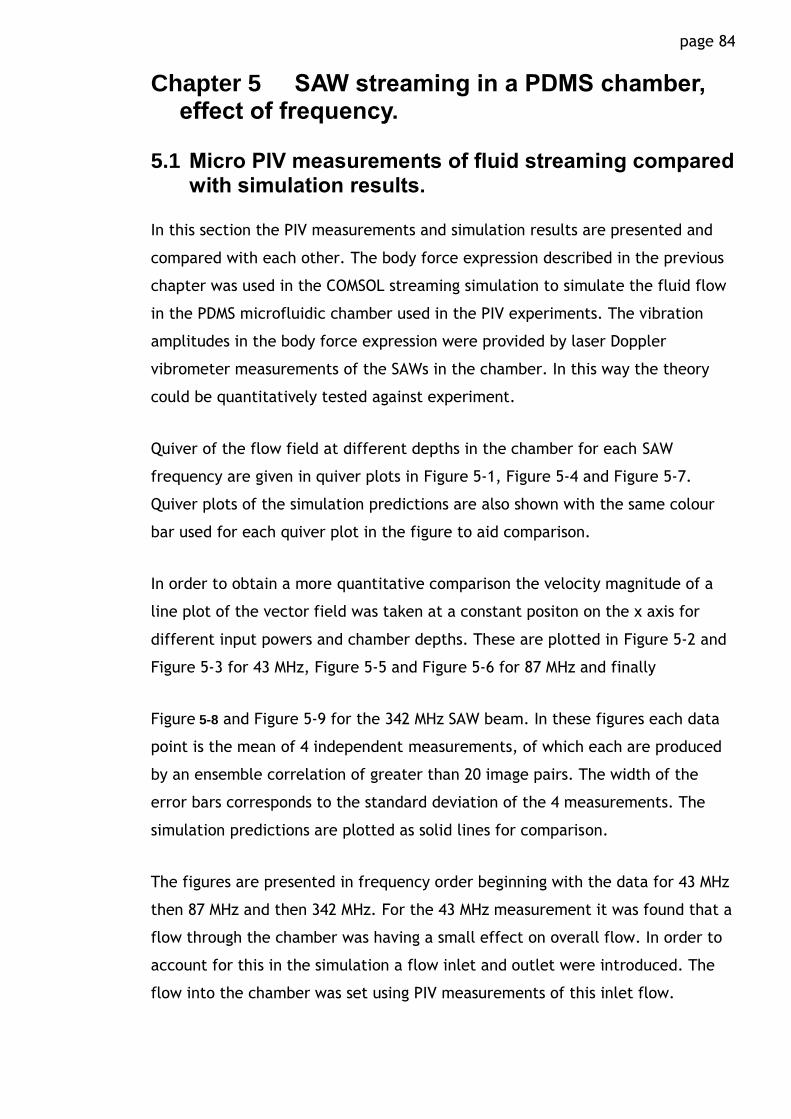
page 84

Chapter 5 SAW streaming in a PDMS chamber, effect of frequency.

5.1 Micro PIV measurements of fluid streaming compared with simulation results.

In this section the PIV measurements and simulation results are presented and

compared with each other. The body force expression described in the previous

chapter was used in the COMSOL streaming simulation to simulate the fluid flow

in the PDMS microfluidic chamber used in the PIV experiments. The vibration

amplitudes in the body force expression were provided by laser Doppler

vibrometer measurements of the SAWs in the chamber. In this way the theory

could be quantitatively tested against experiment.

Quiver of the flow field at different depths in the chamber for each SAW

frequency are given in quiver plots in Figure 5-1, Figure 5-4 and Figure 5-7.

Quiver plots of the simulation predictions are also shown with the same colour

bar used for each quiver plot in the figure to aid comparison.

In order to obtain a more quantitative comparison the velocity magnitude of a

line plot of the vector field was taken at a constant positon on the x axis for

different input powers and chamber depths. These are plotted in Figure 5-2 and

Figure 5-3 for 43 MHz, Figure 5-5 and Figure 5-6 for 87 MHz and finally

Figure 5-8 and Figure 5-9 for the 342 MHz SAW beam. In these figures each data

point is the mean of 4 independent measurements, of which each are produced

by an ensemble correlation of greater than 20 image pairs. The width of the

error bars corresponds to the standard deviation of the 4 measurements. The

simulation predictions are plotted as solid lines for comparison.

The figures are presented in frequency order beginning with the data for 43 MHz

then 87 MHz and then 342 MHz. For the 43 MHz measurement it was found that a

flow through the chamber was having a small effect on overall flow. In order to

account for this in the simulation a flow inlet and outlet were introduced. The

flow into the chamber was set using PIV measurements of this inlet flow.

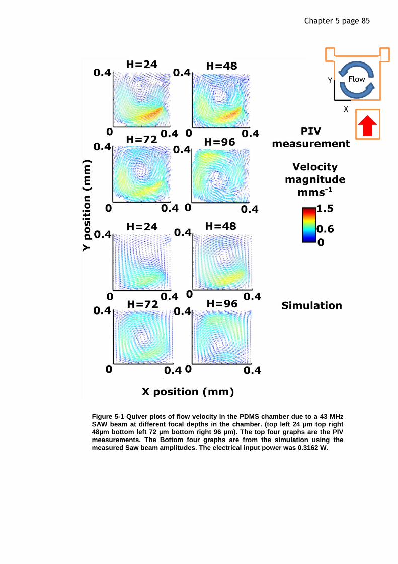
Chapter 5 page 85

X

Figure 5-1 Quiver plots of flow velocity in the PDMS chamber due to a 43 MHz SAW beam at different focal depths in the chamber. (top left 24 µm top right 48µm bottom left 72 µm bottom right 96 µm). The top four graphs are the PIV measurements. The Bottom four graphs are from the simulation using the measured Saw beam amplitudes. The electrical input power was 0.3162 W.

Flow Y

Chapter 5 page 86

Figure 5-2 Velocity magnitude for 43 MHz SAW beam along X=0.2 mm at a depth of 72 μm at different electrical input powers. The width of the error bars is the standard deviation of 4 independent PIV measurements. The line plot shows the in plane velocity magnitude from the simulation.

Figure 5-3 Velocity magnitude for 43 MHz SAW beam along X=0.2 mm with an electrical input power of 0.3162 W. Each plot is a different depth in the chamber. (top left 24 µm top right 48µm bottom left 72 µm bottom right 92 µm) The width of the error bars are the standard deviation of 4 independent PIV measurements.

Chapter 5 page 87

Figure 5-4 Quiver plots of flow velocity in the PDMS chamber due to an 87 MHz SAW beam at different focal depths in the chamber. (top left 24 µm top right 48 µm bottom left 72 µm bottom right 96 µm). The top four graphs are the PIV measurements. The Bottom four graphs are from the simulation using the measured SAW beam amplitudes.

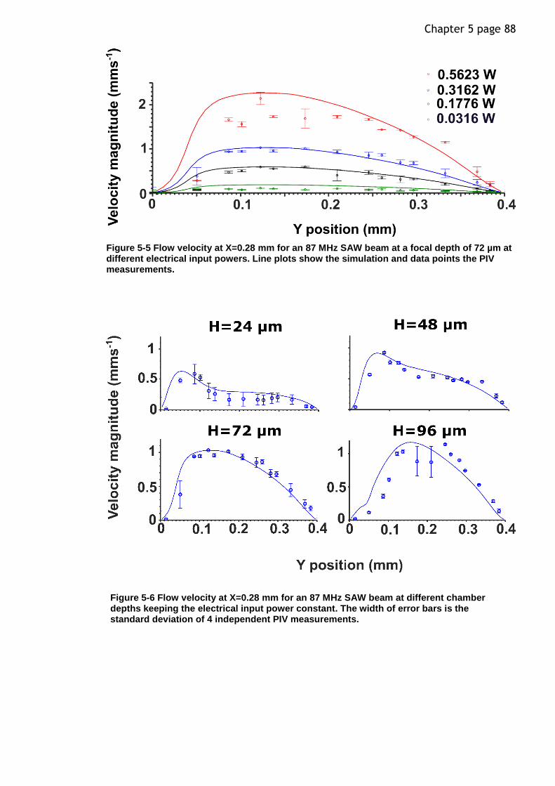
Chapter 5 page 88

Figure 5-6 Flow velocity at X=0.28 mm for an 87 MHz SAW beam at different chamber depths keeping the electrical input power constant. The width of error bars is the standard deviation of 4 independent PIV measurements.

Figure 5-5 Flow velocity at X=0.28 mm for an 87 MHz SAW beam at a focal depth of 72 µm at different electrical input powers. Line plots show the simulation and data points the PIV measurements.

Chapter 5 page 89

Figure 5-7 quiver plots of flow velocity in the PDMS chamber due to a 342 MHz SAW beam at different focal depths in the chamber, (top left 24 µm top right 48 µm bottom left 72 µm bottom right 96 µm). The top four graphs are the PIV measurements. The Bottom four graphs are from the simulation using the measured SAW beam amplitudes.

Chapter 5 page 90

Figure 5-8 Flow velocity at X=0.2 mm for a 342 MHz SAW beam at different input powers. The focal depth in the chamber is 48 μm. The width of the error bars is the standard deviation of 4 independent PIV measurements

Figure 5-9 Flow velocity at X=0.2 mm for a 342 MHz SAW beam at different focal depths in the chamber keeping the input power constant at 0.1 W. The width of the error bars is the standard deviation of 4 independent PIV measurements.

Chapter 5 page 91

The quiver plots show the in plane streaming at different focal depths in the

chamber. At a focal depth of 24 µm, the fluid is being pushed away from the

substrate surface in the bottom right hand corner of the chamber by the body

force on fluid. This is observed in the PIV measurements as a ‘sink’ like area

where the fluid is being dragged upwards and the surrounding fluid is rushing in

to replace it. Further away from the substrate surface an anti-clockwise fluid

vortex is observed, due to the spatial anisotropy of the SAW beam, which

propagates only through the right half of the chamber. Near the roof of the

chamber the upwards motion of the fluid is deflected and there are again

regions where the fluid is pushed further downwards into the chamber that

appear as ‘sink’ like regions.

For the 342 MHz SAW beam there is a large spatial variation in the streaming

magnitude with much faster streaming found close to the point at which the

beam enters the chamber. This makes sense, since the attenuation length at 342

MHz is ~0.2 mm, half the length of the chamber. The 87 MHz and 43 MHz SAW

beams exhibit a much greater spatial homogeneity of streaming magnitudes

across the chamber due to the larger attenuation lengths of the SAW beams.

This is further demonstrated in Figure 5-10 where the sound beam generated by

a 43 and 342 MHz SAW beam are compared with a cross sectional slice of the

streaming flows calculated by the simulation. A 3D Plot of the streamlines in the

chamber has been included underneath for comparison. It is clear there is good

agreement between the simulation and the measurements in terms of the

direction and shape of the fluid flows, however there is some underestimation of

the velocity magnitudes for the 43 MHz and 342 MHz SAW beams.

Chapter 5 page 92

Figure 5-10 Comparison of the streaming flows generated by different frequencies of SAW beam. The initial SAW velocity amplitude has been kept constant for each frequency. (top left and right) shows a cross section of the pressure field along Y and Z at 43 MHz and 342 MHz. (Middle left and right) Colour plot of velocity magnitude for the same spatial cross-section. The white arrows show the direction of flow. Note the different colour scales for each plot, the right plot is ~10 times greater for the same initial SAW velocity amplitude. (Bottom left and right) Streamlines of the flow in 3D over the whole microchamber. The colour plot slice shows how the above cross-sections fit into the chamber.

5.1.1 Comparison of streaming magnitudes

Figure 5-11 shows the mean in plane streaming velocity as a funciton of the

intial SAW beam velocity amplitude for each frequency. Each graph shows the

average streaming velocity at a different focal depth in the chamber. There are

two errorbars plotted showing the standard deviation in the streaming velocity

and also the SAW particle velocity measurements.

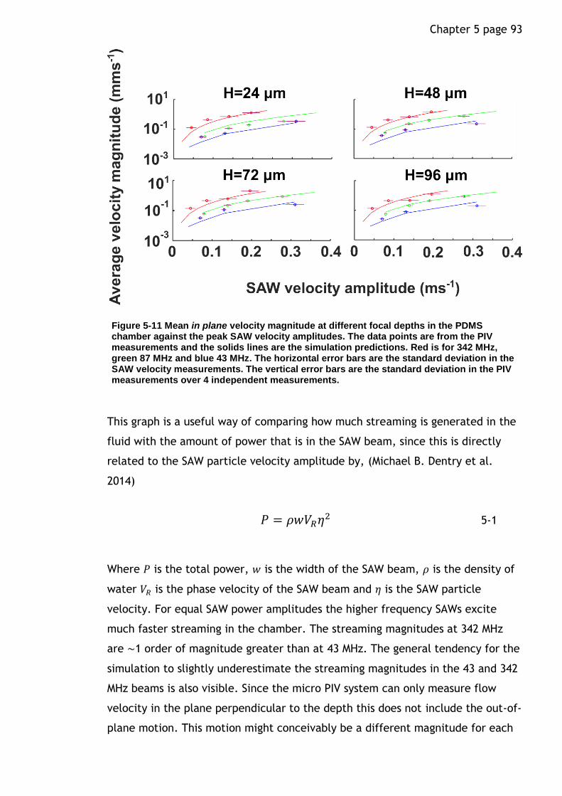
Chapter 5 page 93

This graph is a useful way of comparing how much streaming is generated in the

fluid with the amount of power that is in the SAW beam, since this is directly

related to the SAW particle velocity amplitude by, (Michael B. Dentry et al.

2014)

𝑃 = 𝜌𝑤𝑉𝑅𝜂2 5-1

Where 𝑃 is the total power, 𝑤 is the width of the SAW beam, 𝜌 is the density of

water 𝑉𝑅 is the phase velocity of the SAW beam and 𝜂 is the SAW particle

velocity. For equal SAW power amplitudes the higher frequency SAWs excite

much faster streaming in the chamber. The streaming magnitudes at 342 MHz

are ~1 order of magnitude greater than at 43 MHz. The general tendency for the

simulation to slightly underestimate the streaming magnitudes in the 43 and 342

MHz beams is also visible. Since the micro PIV system can only measure flow

velocity in the plane perpendicular to the depth this does not include the out-of-

plane motion. This motion might conceivably be a different magnitude for each

Figure 5-11 Mean in plane velocity magnitude at different focal depths in the PDMS chamber against the peak SAW velocity amplitudes. The data points are from the PIV measurements and the solids lines are the simulation predictions. Red is for 342 MHz, green 87 MHz and blue 43 MHz. The horizontal error bars are the standard deviation in the SAW velocity measurements. The vertical error bars are the standard deviation in the PIV measurements over 4 independent measurements.

Chapter 5 page 94

frequency so this is a limitation of this comparison. Another limitation is it was

difficult to exactly control the widths of the SAW beam in the chamber between

frequencies. However the data presented is sufficient to validate the utility of

the simulation, which can now be used to make a more ideal comparison

between frequencies.

5.2 Impact of measurement error

The results show very good qualitative agreements between the simulation flow

and the measured PIV flow. However there is some difference between the

velocity magnitudes. At 43 MHz there is some under estimation of the velocity

magnitudes for the 0.1 W input power of between 50 and 100%. For the 87 MHz

results there is excellent agreement between the simulation and the PIV

measurements, however the results for the 342 MHz transducer also show some

under estimation of the observed velocity magnitudes for parts of the velocity

field which were as a much as 25% for the 24 and 48 μm depth height. Since

there is not a consistent difference between the simulation and experiment, it

seems likely this is due to measurement error.

There are three main sources of measurement error that could have an influence

on the observed and simulated fluid flow. Errors due to the PIV measurements,

errors due to the vibrometer measurements and errors in the simulation due to

either incorrect physical properties or due to the approximate analytical

expression for the fluid body force.

The main source of error in the physical properties used in the simulation would

be due to temperature differences. The measurements were performed at room

temperature which was ~ 20±3 °C while the simulation parameters were set at

20 °C. A possible source of error could come from the heating of the water in

the chamber by the SAW beam. Although it is possible to measure the

temperature of the water before insertion, it is difficult to assess the

temperature of the water in the chamber due to the potential heating impact of

the SAW beam, this creates a possible uncertainty in the measurement. To

assess the impact of temperature on the measurement the simulation was run

for values of attenuation, propagation velocity, viscosity and density at different

temperatures. A cross sectional velocity profile is plotted in Figure 5-12.

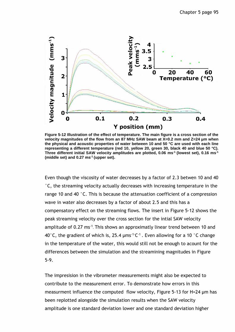
Chapter 5 page 95

Figure 5-12 Illustration of the effect of temperature. The main figure is a cross section of the velocity magnitudes of the flow from an 87 MHz SAW beam at X=0.2 mm and Z=24 μm when the physical and acoustic properties of water between 10 and 50 °C are used with each line representing a different temperature (red 10, yellow 20, green 30, black 40 and blue 50 °C). Three different initial SAW velocity amplitudes are plotted, 0.06 ms-1 (lowest set), 0.16 ms-1

(middle set) and 0.27 ms-1 (upper set).

Even though the viscosity of water decreases by a factor of 2.3 betwen 10 and 40

°C, the streaming velocity actually decreases with increasing temperature in the

range 10 and 40 °C. This is because the attenuation coefficient of a compression

wave in water also decreases by a factor of about 2.5 and this has a

compensatory effect on the streaming flows. The insert in Figure 5-12 shows the

peak streaming velocity over the cross section for the intial SAW velocity

amplitude of 0.27 ms-1. This shows an approximatly linear trend between 10 and

40°C, the gradient of which is, 25.4 µms-1◦C-1 . Even allowing for a 10 °C change

in the temperature of the water, this would still not be enough to acount for the

differences between the simulation and the streamining magnitudes in Figure

5-9.

The impresision in the vibrometer measurements might also be expected to

contribute to the measurement error. To demonstrate how errors in this

measurment influence the computed flow velocity, Figure 5-13 for H=24 µm has

been replotted alongside the simulation results when the SAW velocity

amplitude is one standard deviation lower and one standard deviation higher

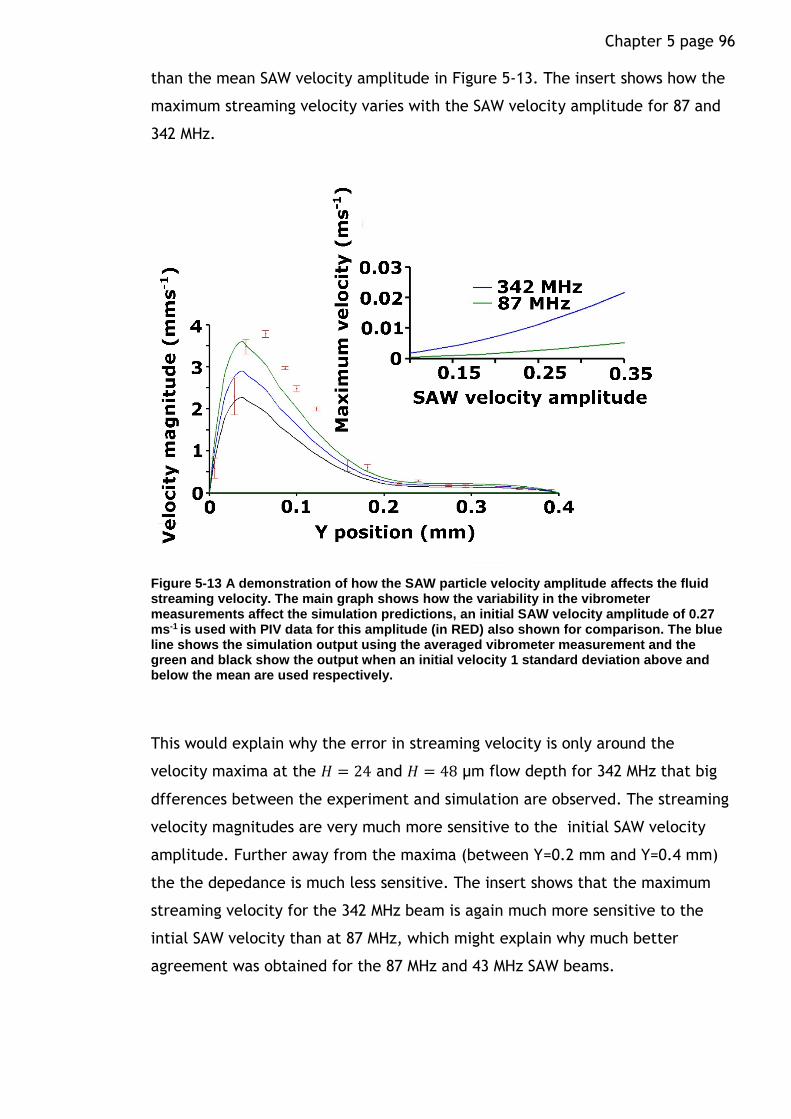
Chapter 5 page 96

than the mean SAW velocity amplitude in Figure 5-13. The insert shows how the

maximum streaming velocity varies with the SAW velocity amplitude for 87 and

342 MHz.

Figure 5-13 A demonstration of how the SAW particle velocity amplitude affects the fluid streaming velocity. The main graph shows how the variability in the vibrometer measurements affect the simulation predictions, an initial SAW velocity amplitude of 0.27 ms-1 is used with PIV data for this amplitude (in RED) also shown for comparison. The blue line shows the simulation output using the averaged vibrometer measurement and the green and black show the output when an initial velocity 1 standard deviation above and below the mean are used respectively.

This would explain why the error in streaming velocity is only around the

velocity maxima at the 𝐻 = 24 and 𝐻 = 48 μm flow depth for 342 MHz that big

dfferences between the experiment and simulation are observed. The streaming

velocity magnitudes are very much more sensitive to the initial SAW velocity

amplitude. Further away from the maxima (between Y=0.2 mm and Y=0.4 mm)

the the depedance is much less sensitive. The insert shows that the maximum

streaming velocity for the 342 MHz beam is again much more sensitive to the

intial SAW velocity than at 87 MHz, which might explain why much better

agreement was obtained for the 87 MHz and 43 MHz SAW beams.

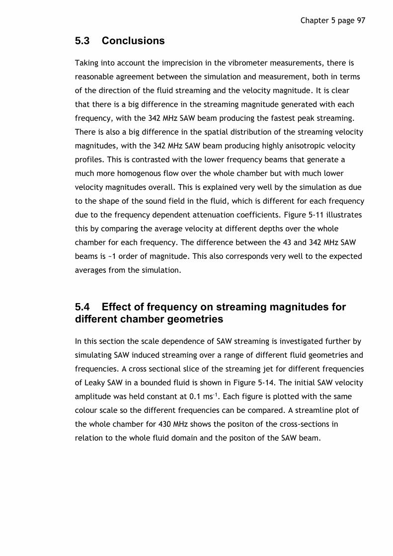
Chapter 5 page 97

5.3 Conclusions

Taking into account the imprecision in the vibrometer measurements, there is

reasonable agreement between the simulation and measurement, both in terms

of the direction of the fluid streaming and the velocity magnitude. It is clear

that there is a big difference in the streaming magnitude generated with each

frequency, with the 342 MHz SAW beam producing the fastest peak streaming.

There is also a big difference in the spatial distribution of the streaming velocity

magnitudes, with the 342 MHz SAW beam producing highly anisotropic velocity

profiles. This is contrasted with the lower frequency beams that generate a

much more homogenous flow over the whole chamber but with much lower

velocity magnitudes overall. This is explained very well by the simulation as due

to the shape of the sound field in the fluid, which is different for each frequency

due to the frequency dependent attenuation coefficients. Figure 5-11 illustrates

this by comparing the average velocity at different depths over the whole

chamber for each frequency. The difference between the 43 and 342 MHz SAW

beams is ~1 order of magnitude. This also corresponds very well to the expected

averages from the simulation.

5.4 Effect of frequency on streaming magnitudes for different chamber geometries

In this section the scale dependence of SAW streaming is investigated further by

simulating SAW induced streaming over a range of different fluid geometries and

frequencies. A cross sectional slice of the streaming jet for different frequencies

of Leaky SAW in a bounded fluid is shown in Figure 5-14. The initial SAW velocity

amplitude was held constant at 0.1 ms-1. Each figure is plotted with the same

colour scale so the different frequencies can be compared. A streamline plot of

the whole chamber for 430 MHz shows the positon of the cross-sections in

relation to the whole fluid domain and the positon of the SAW beam.

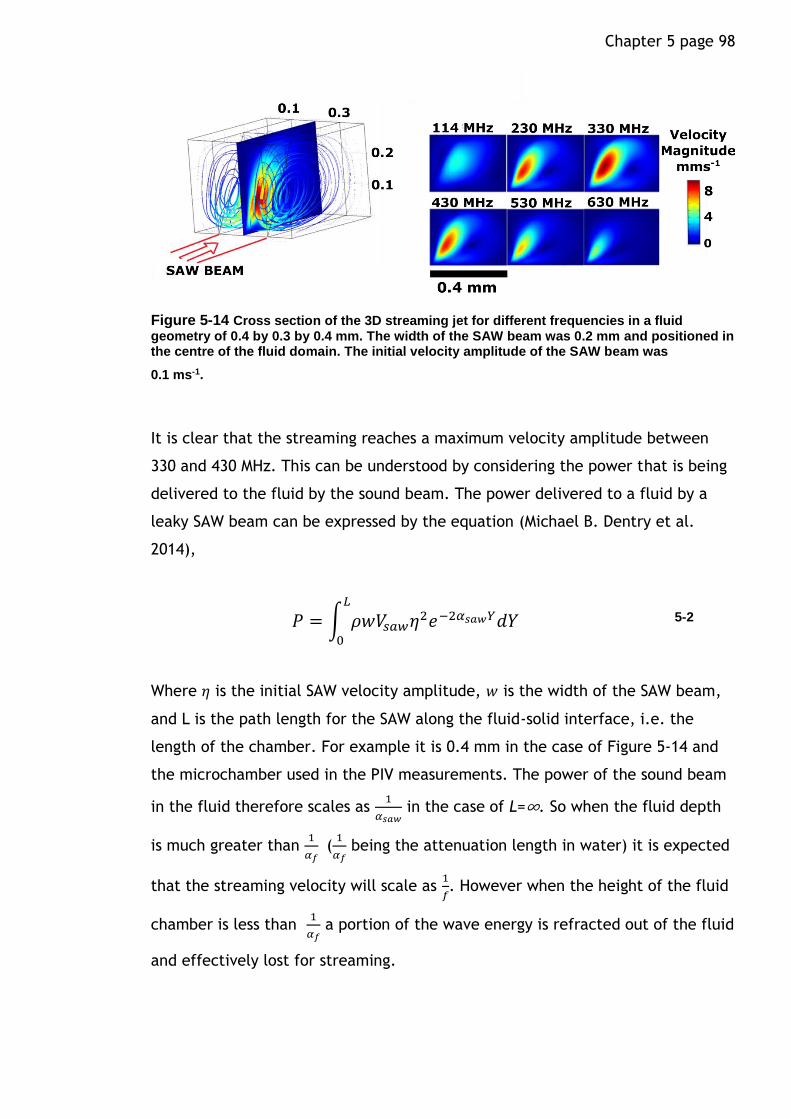
Chapter 5 page 98

Figure 5-14 Cross section of the 3D streaming jet for different frequencies in a fluid geometry of 0.4 by 0.3 by 0.4 mm. The width of the SAW beam was 0.2 mm and positioned in the centre of the fluid domain. The initial velocity amplitude of the SAW beam was

0.1 ms-1.

It is clear that the streaming reaches a maximum velocity amplitude between

330 and 430 MHz. This can be understood by considering the power that is being

delivered to the fluid by the sound beam. The power delivered to a fluid by a

leaky SAW beam can be expressed by the equation (Michael B. Dentry et al.

2014),

𝑃 = ∫ 𝜌𝑤𝑉𝑠𝑎𝑤𝜂2𝑒−2𝛼𝑠𝑎𝑤𝑌𝑑𝑌

𝐿

0

5-2

Where 𝜂 is the initial SAW velocity amplitude, 𝑤 is the width of the SAW beam,

and L is the path length for the SAW along the fluid-solid interface, i.e. the

length of the chamber. For example it is 0.4 mm in the case of Figure 5-14 and

the microchamber used in the PIV measurements. The power of the sound beam

in the fluid therefore scales as 1

𝛼𝑠𝑎𝑤 in the case of L=∞. So when the fluid depth

is much greater than 1

𝛼𝑓 (

1

𝛼𝑓 being the attenuation length in water) it is expected

that the streaming velocity will scale as 1

𝑓. However when the height of the fluid

chamber is less than 1

𝛼𝑓 a portion of the wave energy is refracted out of the fluid

and effectively lost for streaming.

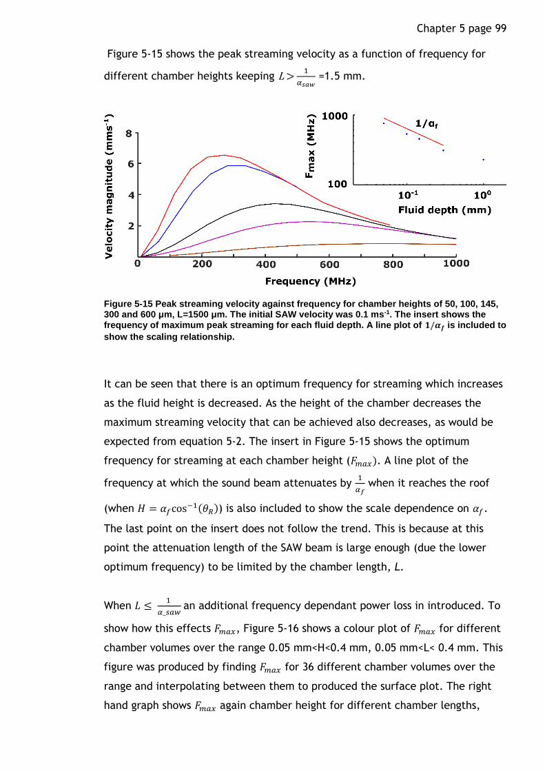
Chapter 5 page 99

Figure 5-15 shows the peak streaming velocity as a function of frequency for

different chamber heights keeping L > 1

𝛼𝑠𝑎𝑤 =1.5 mm.

Figure 5-15 Peak streaming velocity against frequency for chamber heights of 50, 100, 145, 300 and 600 μm, L=1500 μm. The initial SAW velocity was 0.1 ms-1. The insert shows the frequency of maximum peak streaming for each fluid depth. A line plot of 𝟏/𝜶𝒇 is included to

show the scaling relationship.

It can be seen that there is an optimum frequency for streaming which increases

as the fluid height is decreased. As the height of the chamber decreases the

maximum streaming velocity that can be achieved also decreases, as would be

expected from equation 5-2. The insert in Figure 5-15 shows the optimum

frequency for streaming at each chamber height (𝐹𝑚𝑎𝑥). A line plot of the

frequency at which the sound beam attenuates by 1

𝛼𝑓 when it reaches the roof

(when 𝐻 = 𝛼𝑓cos−1(𝜃𝑅)) is also included to show the scale dependence on 𝛼𝑓.

The last point on the insert does not follow the trend. This is because at this

point the attenuation length of the SAW beam is large enough (due the lower

optimum frequency) to be limited by the chamber length, L.

When 𝐿 ≤ 1

𝛼_𝑠𝑎𝑤 an additional frequency dependant power loss in introduced. To

show how this effects 𝐹𝑚𝑎𝑥, Figure 5-16 shows a colour plot of 𝐹𝑚𝑎𝑥 for different

chamber volumes over the range 0.05 mm<H<0.4 mm, 0.05 mm<L< 0.4 mm. This

figure was produced by finding 𝐹𝑚𝑎𝑥 for 36 different chamber volumes over the

range and interpolating between them to produced the surface plot. The right

hand graph shows 𝐹𝑚𝑎𝑥 again chamber height for different chamber lengths,

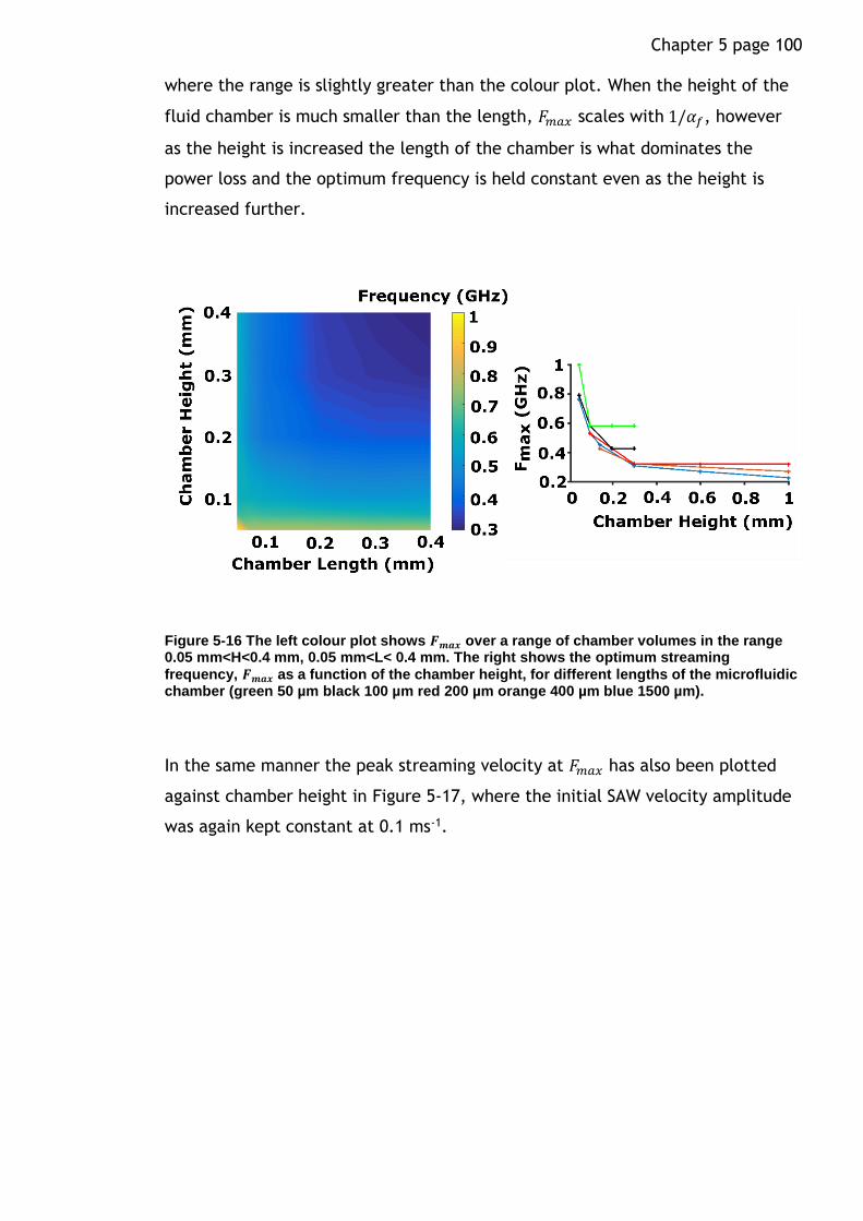
Chapter 5 page 100

where the range is slightly greater than the colour plot. When the height of the

fluid chamber is much smaller than the length, 𝐹𝑚𝑎𝑥 scales with 1/𝛼𝑓, however

as the height is increased the length of the chamber is what dominates the

power loss and the optimum frequency is held constant even as the height is

increased further.

Figure 5-16 The left colour plot shows 𝑭𝒎𝒂𝒙 over a range of chamber volumes in the range 0.05 mm<H<0.4 mm, 0.05 mm<L< 0.4 mm. The right shows the optimum streaming

frequency, 𝑭𝒎𝒂𝒙 as a function of the chamber height, for different lengths of the microfluidic chamber (green 50 µm black 100 µm red 200 µm orange 400 µm blue 1500 µm).

In the same manner the peak streaming velocity at 𝐹𝑚𝑎𝑥 has also been plotted

against chamber height in Figure 5-17, where the initial SAW velocity amplitude

was again kept constant at 0.1 ms-1.

Chapter 5 page 101

Figure 5-17 The left colour plot shows the peak streaming velocity over the range 0.05 mm<H<0.4 mm, 0.05 mm<L< 0.4 mm, the initial SAW amplitude velocity was kept constant at

0.1 ms-1. The right hand graph shows the peak streaming velocity for 𝑭𝒎𝒂𝒙 against chamber height for different chamber lengths (blue 1500 µm red 200 µm black 100 µm green 50 µm).

The maximum streaming velocities achievable are constrained by the fluid

geometry, with peak flow velocity greatly deteriorating as the chamber height

and length are decreased.

Power loss due to PDMS wall

There is also another consideration which is the additional power loss of the SAW

beam along the path before it gets to the fluid chamber. This depends on the

particular set-up but it is hard to imagine when the beam won’t have to travel

across some sort of barrier to get to the fluid. In this study the SAW beam had to

travel across a 0.1 mm thick PDMS wall to get to the fluid. Since this attenuation

is also frequency dependent, it will have an influence on the optimum choice of

frequency and microfluidic geometry. Assuming an attenuation coefficient of

𝛼𝑝𝑑𝑚𝑠 (from the previous chapter) a more realistic simulation would be start

with an initial SAW velocity of 0.1 ms-1 attenuate that by 𝜂 = 𝜂0𝑒−𝛼𝑝𝑑𝑚𝑠𝑑 and

then use 𝜂 as the SAW velocity amplitude in the body force calculation.

Figure 5-18 shows the peak streaming velocity against frequency for a PDMS

micro chamber with a height of 0.3 mm and a length of 0.4 mm after the SAW

beam has crossed different thicknesses of PDMS wall.

Chapter 5 page 102

Figure 5-18 Peak streaming velocity in a chamber of L=0.4 mm and height=0.3 mm when the SAW beam has to initially cross a PDMS wall to get to the fluid. The SAW beam loses a portion of its energy to the wall resulting in slower streaming velocities, since the portion of energy lost to the PDMS wall is frequency dependent this effects the optimum frequency for streaming.

5.5 Conclusions and outlook

Limitations of the simulation

The streaming theory that has been used here is really just the Eckart or ‘bulk’

stremaing detailed in chapter 2. There are two other forms of acoustic

streaming that might contribute to the overall flow. One is due to the vibration

of the leaky SAW itself, which can cause boundary streaming parralel with the

surface. The vibration of leaky SAWs is particulary unusual, as first pointed out

by (Bradley 1996) in that the boundary vibration is spatiotemporaly varible, as

opposed the well studied boundary streaming from rectilinear vibrations of bulk

mode resonators (Hamilton et al. 2003; Lei et al. 2013). (Bradley 1996) showed

that this leads the unique possibility of a slip flow parallel with the boundary.

This has been investigated further by (Vanneste & Buhler 2010) who have

modelled the streaming due to a leaky SAW from both the Eckart and the leaky

SAW boundary in the sagital plane (i.e in two dimentions, parallel with the SAW

propagation and with depth into the fluid). They found that the bulk streaming

was 3-4 orders of magnitude greater when the fluid depth was two orders of

magnitude greater than the wavelength, therefore dominating the overall fluid

Chapter 5 page 103

velocity field. They compared this to when the height was reduced to 10

wavelengths and found that the boundary streaming contributions remained the

same whereas the bulk streaming was greatly reduced, althought still 10 times

greater in magnitude. It is important to point out that this is theoretical only

and there has been no systematic experimental observations of the boundary

streaming occuring from leaky SAWs. It appears from (Vanneste & Buhler 2010)

that one would only expect to see this flow in instances where the fluid

geometry is sufficiently small. Which is not the case for experiments performed

in this thesis.

The other possibility is that as the sound beam grazes the PDMS wall it should

produce boundary streaming at the wall (Nyborg 1965; Chun P & Taylor G 1989).

The relative contribution of this boundary layer streaming against the bulk

streaming again depends on the lengh scale of the microfluidc geometry.

(Frampton et al. 2003) has investigated this theoretically for a plane acoustic

wave in a microfluidic channel with a special interest in the relative

contributions from the buk streaming and boundary layer streaming to the

overall flow. Similar to the leaky SAW vibrations, as the length of the channel

decreases the boundary layer streaming becomes increasingly important. This is

because the magnitude of the bulk streaming scales with the channel length

whereas the bondary layer streaming is independent of the channel size.

In the experimental fluid geometry considered in this chapter contributions from

boundary layer streaming should be neglegable since the height and length of

the chamber are at least 4 times greater than the wavelength in the case of 43 a

MHz and 38 times in the case the 342 MHz SAW beams. In the general case, the

simulation that has been built in this chapter should be sufficiently accurate

only when Eckart streaming dominates the fluid flow. This should be the case

when the fluid length scale is at least five times greater than the wavelength of

the compression wave in the fluid.

In this study the possibility of scattering of the acoustic waves from the walls

and roof of the PDMS chamber have also been ignored to make the analysis

simple. This is considered to be justified, because the PDMS, having an acoustic

impedance similar to water should not strongly reflect waves back into the

chamber.

Chapter 5 page 104

Conclusions

In conclusion, a compuational simulation capable of describing streaming by

leaky SAWs in small fluid geometries was tested again experimental observations

of streaming flows in a microchamber in this chapter. There was good agreement

between the observations and the simulation.

The computational simulation was then used to investigate the relationship

between frequency and streaming velocity for different chamber dimensions. It

was found that as the chamber dimensions decrease the optimum frequency for

streaming increases, dependent on both the length and the height of the

chamber. It was found that for typical microfluidic length scales of 10~100 μm

the optimum frequency for streaming should be 2-3 times greater than is

typicaly used in the literature. It was also found that as the chamber dimensions

become small, the maximum streaming velocity acheivable is greatly reduced.

This information should be useful for the optimal design of SAW streaming in

potential applications such as particle sorting (Franke et al. 2009) and efficient

low Reynolds number mixing.

page 105

Chapter 6 A first step towards an ultrasonic glucose sensor.

6.1 Introduction and overview

In this chapter the physical principles of how an ultrasonic glucose sensing

system based on reflections from a subcutaneous implant might work are

discussed in detail. The basic physical principles are first introduced by

simulating the acoustic reflection spectrum from a one dimensional stack of

layers, this was done using the transfer matrix method described in the

background theory chapter. Then a more complete model based on the KLM

equivalent circuit model is used to simulate the measured response from a

system including the transducers and the skin layer. This makes it possible to

predict the interaction between a transducer and the layered structure. To

consider the effect of incidence angle, a 2D FEM simulation of the acoustic

scattering in both the fluid and solid domains was created (Comsol Inc n.d.).

The theory of acoustic plane wave reflections from different arrangements of

layered acoustic media have been very thoroughly studied over a wide variety of

different research interests. Theoretical expressions have been derived for the

reflection coefficient from single elastic plates immersed in a liquid (Fiorito et

al. 1979) and liquid layers (Überall 1964) as well as many techniques to

investigate the reflection coefficient from a series of layers. A popular and

versatile method is the transmission matrix technique (Lowe 1995) which can be

extended to investigating layers of both liquid and elastic material (Cervenka &

Pascal Challande 1991) and also porous layers (Allard et al. 1993). Examples of

experiments measuring the ultrasonic reflection coefficient from different layers

of elastic plates in water can be found in (Lenoir 1992) and (Folds & Loggins

1977).

The reflection spectrum of ultrasonic waves from layered media has been given

considerable attention from many different branches of work focusing on

achieving solutions to different engineering problems. In ultrasonic non-

destructive testing (NDT), embedded layers which are too thin to be properly

resolved with time of flight measurements have been characterised using the

Chapter 6 page 106

spectrum of reflected waves. This was first investigated in (Pialucha et al. 1989)

who looked at the reflection spectrum from a single metal plate in a water bath.

The ultrasonic reflection spectrum has been used to measure the thickness of a

lubricant film between two metal plates. Measurement of the thickness of the

lubricant film was possible down to 10 μm by examining the resonance frequency

of the liquid layer (Dwyer-Joyce et al. 2003). The reflection spectrum from a

more complex 3 layered structure consisting of a thin adhesive layer between

two metal plates in a water bath has also been thoroughly investigated with the

interest being able to infer the thickness and acoustic impedance of a bond joint

(Hanneman & Kinra 1992).

Recently there has also been much interest in phononic crystals, because of

their potential use as waveguides (Wilson et al. 2011) (Otsuka et al. 2013),

frequency filters (Lee et al. 2013) (Benchabane et al. 2006) and as sensors

(Lucklum et al. 2012) (Ke et al. 2011). Phononic crystals are metamaterials that

have a spatial periodicity in their acoustic impedance, this could form 1D, 2D or

3D patterns (Yang et al. 2004). A particularly interesting feature of phononic

crystals is that they can be engineered to produce wide frequency bands in

which wave propagation through the structure is completely prohibited. By

introducing defects into this pattern (a layer where the pattern is broken) it is

possible to create very sharp single transmission peaks in the stop band, the

frequency of which is very sensitive to the properties of the defect layer (Wu et

al. 2009).

It has been argued that these sharp resonances can be exploited as sensing

platforms where the defect layer in a finite phononic pattern becomes the

‘sensing’ layer. Changes in the physical properties of this layer alter the

frequency position of the transmission peak (Ke et al. 2011; Lucklum et al. 2012;

Lucklum & Li 2009; Wang 2010). The rationale behind this is the exploitation of

the very sharp transmission peak that is created in the middle of the stop band

by the defect layer. If this defect layer is a fluid for example it could form the

basis for a chemical sensing strategy.

In this work these ideas serve as the inspiration for an acoustic system that could

sense changes in glucose concentration by using ultrasonic waves to interrogate

the physical state of a glucose sensitive implant. Figure 6-1 shows a schematic of

Chapter 6 page 107

the in vivo system that is the eventual aim of this work. An alternating electric

signal is sent to an ultrasonic transducer where part of the signal is converted to

ultrasonic pressure waves which propagate through the layered system. A series

of reflections and refractions through all the different materials in the medium

eventually lead to a fraction of the total acoustic energy being reflected back to

the transducer. The possible inclusion of an additional layered structure could

be used as a reference measurement.

Figure 6-1 An Illustration of the ultrasonic sensing concept. An ultrasonic transducer emits a spectrum of plane pressure waves through the skin which reflect off the implant and records the amplitude or the phase of the reflections, which will be dependent on the mechanical properties of the implanted device. The device contains an acoustic layer that changes its acoustic impedance properties based on glucose concentration. A static structure is used as a reference measurement. The image is intended as a conceptual aid, and is not literal.

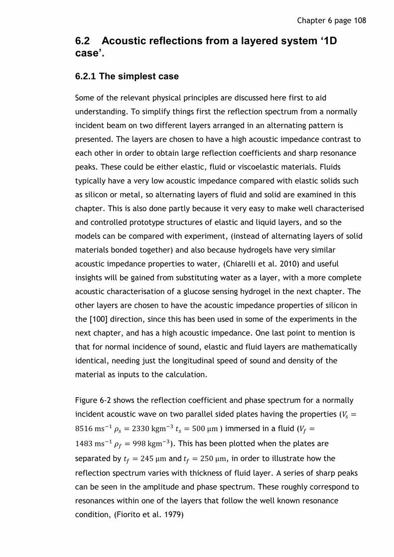
Chapter 6 page 108

6.2 Acoustic reflections from a layered system ‘1D case’.

6.2.1 The simplest case

Some of the relevant physical principles are discussed here first to aid

understanding. To simplify things first the reflection spectrum from a normally

incident beam on two different layers arranged in an alternating pattern is

presented. The layers are chosen to have a high acoustic impedance contrast to

each other in order to obtain large reflection coefficients and sharp resonance

peaks. These could be either elastic, fluid or viscoelastic materials. Fluids

typically have a very low acoustic impedance compared with elastic solids such

as silicon or metal, so alternating layers of fluid and solid are examined in this

chapter. This is also done partly because it very easy to make well characterised

and controlled prototype structures of elastic and liquid layers, and so the

models can be compared with experiment, (instead of alternating layers of solid

materials bonded together) and also because hydrogels have very similar

acoustic impedance properties to water, (Chiarelli et al. 2010) and useful

insights will be gained from substituting water as a layer, with a more complete

acoustic characterisation of a glucose sensing hydrogel in the next chapter. The

other layers are chosen to have the acoustic impedance properties of silicon in

the [100] direction, since this has been used in some of the experiments in the

next chapter, and has a high acoustic impedance. One last point to mention is

that for normal incidence of sound, elastic and fluid layers are mathematically

identical, needing just the longitudinal speed of sound and density of the

material as inputs to the calculation.

Figure 6-2 shows the reflection coefficient and phase spectrum for a normally

incident acoustic wave on two parallel sided plates having the properties (𝑉𝑠 =

8516 ms−1 𝜌𝑠 = 2330 kgm−3 𝑡𝑠 = 500 μm ) immersed in a fluid (𝑉𝑓 =

1483 ms−1 𝜌𝑓 = 998 kgm−3). This has been plotted when the plates are

separated by 𝑡𝑓 = 245 μm and 𝑡𝑓 = 250 μm, in order to illustrate how the

reflection spectrum varies with thickness of fluid layer. A series of sharp peaks

can be seen in the amplitude and phase spectrum. These roughly correspond to

resonances within one of the layers that follow the well known resonance

condition, (Fiorito et al. 1979)

Chapter 6 page 109

𝐹𝑓𝑚 =

𝑚𝑉𝑓2𝑡𝑓

6-1

or

𝐹𝑆𝑚 =

𝑚𝑉𝑠2𝑡𝑆

6-2

Where 𝑉𝑓 and 𝑡𝑓 are thickness and phase velocity in the fluid layer and 𝑉𝑠 and 𝑡𝑠

are the phase velocity and thickness in the plates and m is an integer. This is the

condition for perfect interference of the reflected waves, i.e. the superposition

of the successive reflected waves from the front and the back end of the plate,

for a single plate immersed in a fluid with a normal incidence of sound these

equations are exact, however where there are multiple layers these are rules of

thumb rather than absolutes as the exact position of each resonance is weakly

dependent on the properties of all the layers. The resonance at 𝐹𝑠1, for example

corresponds with the first plate layer. The resonance for the second plate layer

is shifted either up or down by the interference from the layers in front of it.

This is why there are two semi-overlapping peaks close to the 𝐹𝑠1 given by

equation 6-2.

Figure 6-2 The Reflection coefficient (top) and phase spectrum (bottom) are plotted against frequency for a simple three layer structure consisting of two silicon layers in water as illustrated on the left using the chain matrix technique with no reflection boundary

conditions. This has been for plotted for 𝑻𝒇 = 𝟐𝟒𝟓 and 𝟐𝟓𝟎 μm to show how this changes

the position of the peaks. The incident wave comes in from infinity from the left.

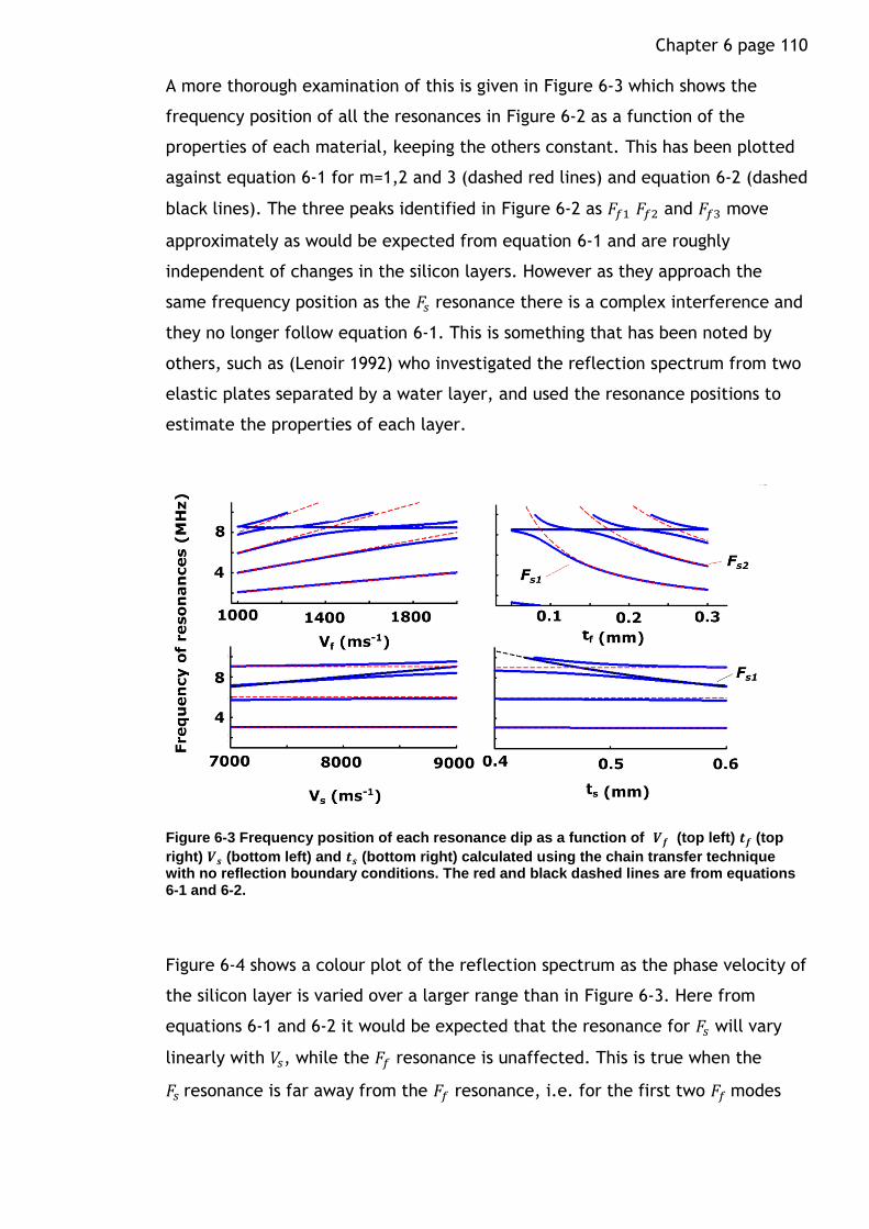
Chapter 6 page 110

A more thorough examination of this is given in Figure 6-3 which shows the

frequency position of all the resonances in Figure 6-2 as a function of the

properties of each material, keeping the others constant. This has been plotted

against equation 6-1 for m=1,2 and 3 (dashed red lines) and equation 6-2 (dashed

black lines). The three peaks identified in Figure 6-2 as 𝐹𝑓1 𝐹𝑓2 and 𝐹𝑓3 move

approximately as would be expected from equation 6-1 and are roughly

independent of changes in the silicon layers. However as they approach the

same frequency position as the 𝐹𝑠 resonance there is a complex interference and

they no longer follow equation 6-1. This is something that has been noted by

others, such as (Lenoir 1992) who investigated the reflection spectrum from two

elastic plates separated by a water layer, and used the resonance positions to

estimate the properties of each layer.

Figure 6-3 Frequency position of each resonance dip as a function of 𝑽𝒇 (top left) 𝒕𝒇 (top

right) 𝑽𝒔 (bottom left) and 𝒕𝒔 (bottom right) calculated using the chain transfer technique with no reflection boundary conditions. The red and black dashed lines are from equations 6-1 and 6-2.

Figure 6-4 shows a colour plot of the reflection spectrum as the phase velocity of

the silicon layer is varied over a larger range than in Figure 6-3. Here from

equations 6-1 and 6-2 it would be expected that the resonance for 𝐹𝑠 will vary

linearly with 𝑉𝑠, while the 𝐹𝑓 resonance is unaffected. This is true when the

𝐹𝑠 resonance is far away from the 𝐹𝑓 resonance, i.e. for the first two 𝐹𝑓 modes

Chapter 6 page 111

when 𝑉𝑠 > 8000 ms−1. However as 𝑉𝑠 decreases there is a strong interaction

between the two resonances.

Figure 6-4 Colour plot of the reflection spectrum as a function of the speed of sound in the silicon layer. As the 𝑭𝒔resonance approaches an 𝑭𝒇 resonance a complicated interaction

occurs. As 𝑭𝒔 increases the 𝑭𝒇 resonances approach the values given by equation 6-1.

The acoustic impedance contrast between the two layers affects the width of

the resonances, with a high contrast leading to sharper resonances. This is

demonstrated in Figure 6-5 where the impedance of the silicon layer is varied

while keeping the phase velocity constant.

Figure 6-5 Reflection spectrum as acoustic impedance of the silicon layer is varied, keeping the phase velocity constant. The resonances get sharper as the acoustic impedance contrast increases.

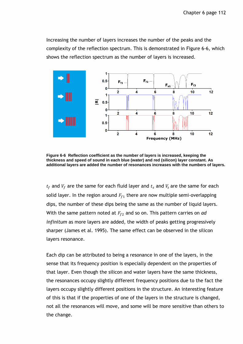
Chapter 6 page 112

Increasing the number of layers increases the number of the peaks and the

complexity of the reflection spectrum. This is demonstrated in Figure 6-6, which

shows the reflection spectrum as the number of layers is increased.

Figure 6-6 Reflection coefficient as the number of layers is increased, keeping the thickness and speed of sound in each blue (water) and red (silicon) layer constant. As additional layers are added the number of resonances increases with the numbers of layers.

𝑡𝑓 and 𝑉𝑓 are the same for each fluid layer and 𝑡𝑠 and 𝑉𝑠 are the same for each

solid layer. In the region around 𝐹𝑓1 there are now multiple semi-overlapping

dips, the number of these dips being the same as the number of liquid layers.

With the same pattern noted at 𝐹𝑓2 and so on. This pattern carries on ad

infinitum as more layers are added, the width of peaks getting progressively

sharper (James et al. 1995). The same effect can be observed in the silicon

layers resonance.

Each dip can be attributed to being a resonance in one of the layers, in the

sense that its frequency position is especially dependent on the properties of

that layer. Even though the silicon and water layers have the same thickness,

the resonances occupy slightly different frequency positions due to the fact the

layers occupy slightly different positions in the structure. An interesting feature

of this is that if the properties of one of the layers in the structure is changed,

not all the resonances will move, and some will be more sensitive than others to

the change.

Chapter 6 page 113

This is demonstrated in more detail in Figure 6-7, where the position of the dips

as the properties of the middle liquid layer is varied and is shown for when there

are 3 liquid layers and 4 solid layers (i.e. the middle graph in Figure 6-6). The

red dashed lines are again from equation 6-1, following the change in either 𝐶𝑙

or 𝑇𝑙. The green dashed lines are also from equation 6-1 where 𝐶𝑙 and 𝑇𝑙 are kept

constant, as in the other water layers. The black dashed lines are again from

equation 6-2. As the properties of the middle layer change a corresponding dip

that follows equation 6-1 can be seen (close to the red dashed line), however

two dips (very close together) remain relatively unmoved, closely described by

equation 1.1 (green dashed line) with 𝐶𝑙 = 1483 ms−1 and 𝑇𝑙 = 250 μm.

Figure 6-7 Position of the resonance peaks for 3 water layers between 4 silicon layers as a

function of 𝑪𝒍 (left) and 𝑻𝒍 (right) in the middle liquid layer. When the resonance frequency of the middle liquid layer is close to the frequency positon of the other layer resonance there is an interaction between the two resonances.

The last few pages give some insight into the possible use of these structures for

sensing changes in one of the layers. Firstly, sharp resonances can be engineered

in the reflection spectrum by using stacked layers of high acoustic impedance

contrast. The frequency position of these resonances will be governed by

equations 6-1 and 6-2, i.e. they can be used to sense changes in the physical

properties of a layer.

Chapter 6 page 114

An important implication is that as the layer thickness decreases the minimum

frequency that can be used for sensing increases. When the layer is imbedded in

a lossy medium it may be more desirable to use low frequencies, since acoustic

attenuation in different mediums scale unfavourably with frequency.

When the resonances from two different layers are close enough to each other in

the frequency spectrum there is an interaction between them that is

complicated and cannot be described using a simple intuitive equation as in

equations 6-1 and 6-2. In this region it becomes very hard to distinguish between

each resonance, and changes in either layer can affect the positon of both

resonances. This coupling of the resonances presents a potential problem for

sensing due to the fact that changes in another layer could affect the

measurement. A way around this might be to engineer the structure so that the

sensing layer resonance is far enough away from other layer resonances in the

frequency spectrum that they do not interact. In the case of a subcutaneous

implant however, it is shown next that this is quite difficult.

KLM model and skin layer

In order to build things further, a model for a transducer is introduced into the

arrangement. This is used to investigate the reflections between the transducer

and the implant via the skin, as a more complete model should include the

transducer and the medium between transducer and implant.

The KLM equivalent circuit model described in the background theory chapter

provides a way of accurately modelling the transduction of an electric signal into

an acoustic wave and vice versa by a piezoelectric element. Including this in the

1D acoustic layer model allows one to go from an electric signal placed across

the transducer to the acoustic transduction of the signal and then the acoustic

reflections and refractions in all the layers (Szabo 2004).

In this section the parameters for a lead metaniobate (𝑃𝑏𝑁𝑏2𝑂6) transducer are

used since this is the transducer that is used in the majority of experiments in

this and the next chapter. The parameters values used for this transducer can be

found the materials and methods chapter. This model is also compared with

experiment in the next chapter.

Chapter 6 page 115

A layer to represent the skin is also introduced between the transducer and the

first silicon layer. The acoustic properties of skin are taken from (Szabo 2004)

(𝜌𝑠𝑘 = 998 kgm−3 𝑉𝑠𝑘 = 1730 ms−1). The thickness has been set as 𝑡𝑠𝑘 = 1.8 mm

which is the typical thickness of human skin (Raj 2002). The simulated reflection

spectrum when the skin layer is introduced between the transducer and implant

is shown in Figure 6-8.

Figure 6-8 (top) Simulated reflection coefficient as measured at the electric input port for a transducer with a 1.8 mm skin layer in between the transducer and the implant chip.

Numerous additional resonances are introduced into the spectrum from the

strong standing wave reflections generated between the transducer face and the

first silicon layer which, like the other layers follow the rule of thumb

𝐹𝑠𝑘𝑚 =𝑚𝑉𝑠𝑘

2𝑡𝑠𝑘, where 𝑉𝑠𝑘 is the phase velocity in the skin and 𝑡𝑠𝑘 is the propagation

distance between the transducer and the skin. The reason that there are so

many is because of the relatively large thickness which shortens the distance in

the frequency spectrum between each mode.

Chapter 6 page 116

The task now is to determine whether it is possible to measure from the

spectrum of the reflected waves, a change in the sensing layer without

interference from changes in any of the other layers. If the implant layers and

the transducer can be built such that they do not change over time, then the

problem is reduced to changes in the skin layer. This might well be expected to

be non-stable, for example knocking the transducer a little, or changes in the

tissue structure due to the foreign body response, or changes in the incidence

angle of the ultrasonic waves, flow and or evaporation of any ultrasonic couplant

used between the transducer and the skin layer etc.

The reflection spectrum as a function of changes in the acoustic properties of

either the skin layer or the water layer are plotted in Figure 6-9 and Figure 6-10

for a 3 layered structure with the same parameters as in Figure 6-8.

Figure 6-9 Colour plot of the magnitude of the reflection coefficient as a function of the phase velocity (left) and thickness (right) of the water layer. The layered system is the same as in Figure 6-8.

As would be expected the resonance peaks due to the skin layer are rather

insensitive to changes in the water layer. It can be seen when the resonance in

the water layer is not close to one of the resonances in the skin layer, it behaves

according to equation 6-1. However as it approaches the frequency position of

one of the other resonances a switch over occurs and in this region it is very

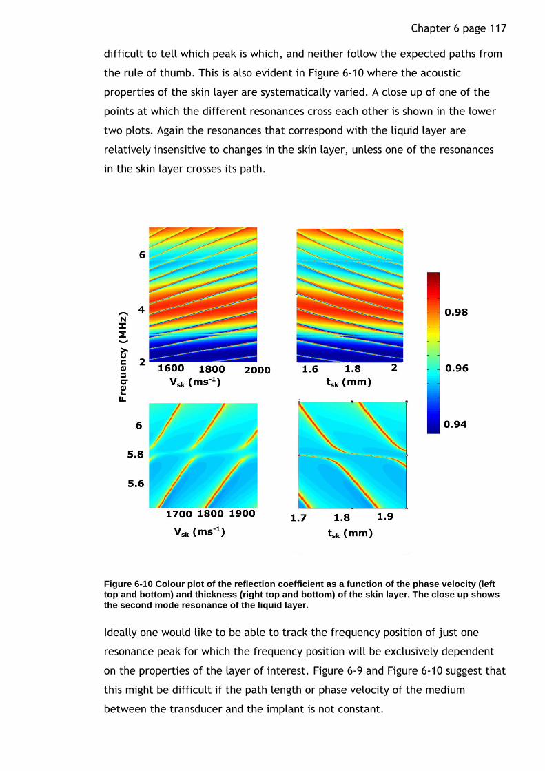
Chapter 6 page 117

difficult to tell which peak is which, and neither follow the expected paths from

the rule of thumb. This is also evident in Figure 6-10 where the acoustic

properties of the skin layer are systematically varied. A close up of one of the

points at which the different resonances cross each other is shown in the lower

two plots. Again the resonances that correspond with the liquid layer are

relatively insensitive to changes in the skin layer, unless one of the resonances

in the skin layer crosses its path.

Figure 6-10 Colour plot of the reflection coefficient as a function of the phase velocity (left top and bottom) and thickness (right top and bottom) of the skin layer. The close up shows the second mode resonance of the liquid layer.

Ideally one would like to be able to track the frequency position of just one

resonance peak for which the frequency position will be exclusively dependent

on the properties of the layer of interest. Figure 6-9 and Figure 6-10 suggest that

this might be difficult if the path length or phase velocity of the medium

between the transducer and the implant is not constant.

Chapter 6 page 118

A solution of this is to embed the sensing layer inside a larger number of layers

as with the 7 layered structures in Figure 6-6. The resonances due to the middle

liquid layer are then much less sensitive to the changes in the skin layer. Figure

6-11 shows a comparison between the reflection spectrum from a 3 and 7 layer

structure as a function of the phase velocity or thickness of the skin layer. The

thickness and impedance of the layered structures are the same as for Figure 6-6

but with the sensing layer set to 150 μm thick (middle layer for the 7 layer

system). For this thickness one expects a resonance at ~4.9 MHz from equation

6-1. The frequency scales on each figure are the same to facilitate comparison.

Figure 6-11 (top left and right) show color plots of the reflecton spectrum in the vicinity of

the 𝑭𝒇𝟏 (𝒕𝒇 = 𝟏𝟓𝟎 𝛍𝐦) resonance for the 3 layer structure as a funciton of the thickness and

phase velocity of the skin layer respectivly. (bottom left and right) show the reflecton

spectrum in the vicinity of the 𝑭𝒇𝟏 resonance for the middle liquid layer of a 7 layer

strucutre as a funciton of the thickness and phase velocity of the skin layer.

The 𝐹𝑓1 peak in the 7 layered system is very sharp as would be expected from

Figure 6-6. Its frequency position is also much less sensitive to the changes in

the skin layer. This is investigated further in Figure 6-12, where the top three

figures show the peak position as a function of the middle liquid layer thickness

for a 3, 7 and 11 layer system using the same material properties as in Figure

6-11. The data points are the maximum and minimum positions of the 𝐹𝑓1

resonance over a variation in skin thickness between 1.3 and 2.3 mm. This is

plotted against equation 6-1 for clarity. The difference between the maximum

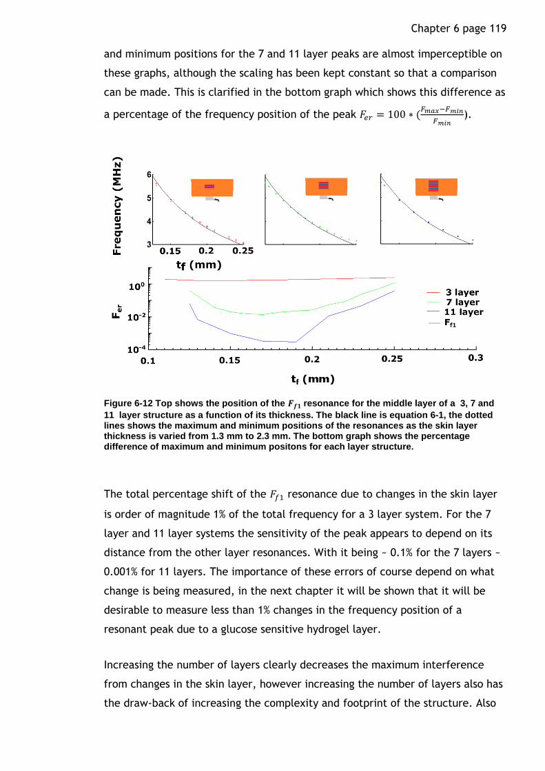
Chapter 6 page 119

and minimum positions for the 7 and 11 layer peaks are almost imperceptible on

these graphs, although the scaling has been kept constant so that a comparison

can be made. This is clarified in the bottom graph which shows this difference as

a percentage of the frequency position of the peak 𝐹𝑒𝑟 = 100 ∗ (𝐹𝑚𝑎𝑥−𝐹𝑚𝑖𝑛

𝐹𝑚𝑖𝑛).

Figure 6-12 Top shows the position of the 𝑭𝒇𝟏 resonance for the middle layer of a 3, 7 and

11 layer structure as a function of its thickness. The black line is equation 6-1, the dotted lines shows the maximum and minimum positions of the resonances as the skin layer thickness is varied from 1.3 mm to 2.3 mm. The bottom graph shows the percentage difference of maximum and minimum positons for each layer structure.

The total percentage shift of the 𝐹𝑓1 resonance due to changes in the skin layer

is order of magnitude 1% of the total frequency for a 3 layer system. For the 7

layer and 11 layer systems the sensitivity of the peak appears to depend on its

distance from the other layer resonances. With it being ~ 0.1% for the 7 layers ~

0.001% for 11 layers. The importance of these errors of course depend on what

change is being measured, in the next chapter it will be shown that it will be

desirable to measure less than 1% changes in the frequency position of a

resonant peak due to a glucose sensitive hydrogel layer.

Increasing the number of layers clearly decreases the maximum interference

from changes in the skin layer, however increasing the number of layers also has

the draw-back of increasing the complexity and footprint of the structure. Also

Chapter 6 page 120

the diffusion path length for the glucose to get to the sensing layer is increased.

This is turn requires that the layers be thinner, which in turn pushes up the

resonance frequencies. The problem with this is that ultrasonic attenuation is

frequency dependent and therefore there will be a point at which reflections

will no longer be detectable over the signal noise.

The next section examines the effect of porosity on the physical properties of

the structure.

Porosity

A general theory of acoustic waves in porous media was first initiated in a series

of papers by Biot (Biot 1962; Biot 1956b; Biot 1956a). This theory has been

applied most widely in geomechanics where it has been used to describe

acoustic wave propagation and attenuation in porous rocks and sediments such

as the ocean bottom (Tokuo 1983). However the theory has also been found to

be widely applicable to many different materials such as gels (Johnson 1982)

consolidated and unconsolidated media (Johnson & Plona 1982) and cancellous

bone (Hosokawa 2005) among others. The most striking consequence of Biot’s

theory is the presence of a third propagating wave mode in a porous material.

This is often referred to as the ‘slow wave’ and is a compression wave, existing

alongside a ‘fast’ compression wave and a shear wave.

The consequences of the theory in the ‘stiff frame’ limit are perhaps the most

important to consider for this thesis, since it is in this limit that the highest

acoustic impedance materials will lie, with unconsolidated and limp frames

tending to be support much lossier waves and these would intuitively be

expected to produce wider, weaker resonances (Johnson et al. 1994). The stiff

frame limit refers to when the porous medium consists of a consolidated,

homogenous elastic frame saturated with a fluid where the bulk and shear

moduli of the frame are much greater than that of the fluid(Johnson & Plona

1982). In the stiff frame limit the fast and slow compression waves can be

interpreted as effectively being separate waves in the fluid (slow) and solid

(fast) parts of the medium. In this limit, the phase velocity expression for each

wave mode is relatively simple,

Chapter 6 page 121

𝑉(𝑓𝑎𝑠𝑡) = (𝐾𝑏 +

43𝑁

(1 − 𝜙)𝜌𝑠 + (1 − 𝛼−1)𝜙𝜌𝑓

)

6-3

𝑉(𝑠𝑙𝑜𝑤) = (𝑉𝑓

√𝛼)

6-4

Where 𝐾𝑏 and 𝑁 are the bulk and shear moduli of the drained elastic frame, 𝜌𝑠

and 𝜌𝑓 are the density of the solid frame and the fluid and 𝛼 is called the

tortuosity and can be interpreted as a measure of the amount of fluid that is

dragged along by the oscillations of the stiff frame (Johnson & Plona 1982). In

the high frequency limit (where the pore size is greater than the viscous skin

depth given by (2𝜂

𝜌𝑓𝜔)

1

2) this is determined by the pore geometry and is a real

valued number greater than 1. As an example it has been measured for sintered

glass beads of varying porosities where it was roughly 𝛼 ∝ 𝜙−1

2 (Johnson et al.

1982). In the low frequency limit viscous effects dominate in the pore and the

slow wave is diffusive. In this limit the fluid in the pores still contributes an

extra factor to the attenuation of the fast and shear waves, which then acts a

bit like a visco-elastic plate (Belloncle et al. 2003).

To properly describe reflection and transmission from a series of layers, some of

them porous, it is necessary to go back the boundary conditions at the interface

between the porous layer and its neighbour (Deresiewicz & Skalak 1963). These

depend of the type of porosity, particularly whether the pores are ‘open’ or

‘closed’ or somewhere in between (Gurevich & Schoenberg 1999). Also the

transmission matrices derived in chapter 2 must be modified to include an

account of the slow wave, and this results in a 4 by 4 transmission matrix when

only considering normal incidence and 6 by 6 matrix when include angled

incidence (and the possible creation of shear waves). For example see, (Allard et

al. 1993).

Chapter 6 page 122

The transmission coefficient of sound through a slab of poroelastic material has

been studied by quite a number of different authors. Theoretical studies of the

reflection properties of water saturated porous glass plate have been performed

in (Belloncle et al. 2003), who showed that in the low frequency limit, where

the slow wave is diffusive, the reflection coefficient resembles that of a

viscoelastic plate. For the higher frequency limit there are extra resonance

modes in the dispersion curve that behave like that of a liquid layer (Franklin et

al. 2010). These exist alongside more recognisable Lamb modes of a viscoelastic

plate.

Recently the use of ultrasound for the characterization of electrochemically

etched porous silicon wafers has received some interest (Da Fonseca et al. 1995;

Bustillo et al. 2014). This has involved measuring the ultrasonic reflection and

transmission spectrum of an electrochemically etched silicon wafer and relating

this back to the porosity of the wafer. These authors were able to reproduce the

reflection spectrum for porous silicon without considering the additional slow

wave mode. None mention a reason in the text, but presumably they are in the

low frequency limit, with diffusive slow waves, since the pores sizes are

typically between 10 and 100 nm. In these works the compression and shear

wave velocity were fitted to a simple empirical model (Da Fonseca et al. 1995),

𝑉𝑙 = 𝑉𝑙𝑜(1 − 𝜙)𝑘 6-5

𝑉𝑠 = 𝑉𝑠0(1 − 𝑃)𝑚 6-6

Where 𝑉𝑙 and 𝑉𝑠 are the longitudinal and shear phase velocity of the porous

silicon, 𝜙 is the porosity, and 𝑘 and 𝑚 are parameters that were determined by

fitting to the empirical data.

Clearly, the particular properties of a porous layer greatly affect its behaviour.

When designing a porous layer for use in the sensing system under investigation

here, it would be desirable to maximise porosity without compromising on the

ability to measure sharp resonances from one of the liquid/hydrogel layers.

Furthermore, interference from the slow wave resonances, which will occupy a

Chapter 6 page 123

similar frequency position because of their similar phase velocity would be very

undesirable due to the interference coupling. Therefore it is likely that the most

appropriate porous material will be ones operating ideally in the low frequency

limit, i.e. where the pore size is much smaller than the viscous skin depth, to

eliminate slow wave interference. This would require typical pore sizes of

around 1-100 nm at MHz frequencies. The effect of increasing porosity would be

to decrease the effective impedance of the material, which will widen and

weaken the resonance peaks of interest, which is undesirable and in the extreme

will make it impossible to accurately measure the position of the resonances. So

there is trade off required between porosity and acoustic impedance contrast.

6.3 Incidence angle

A ‘2D’ COMSOL model is used to examine the reflection as a function of the

incidence angle of the ultrasonic beam. When the incident wave is not normal to

the layered structure a portion of the wave will excite shear waves in the elastic

layers as well as longitudinal waves. When the thickness of these layers is less

than a few wavelength the wave modes of the elastic layers are properly

described as lamb waves (Fiorito et al. 1979).

The transmission resonances in the plate now no longer obey equation 6-2 since

at the boundary there are two overlapping waves modes (shear and

longitudinal). Instead, when there is a large acoustic impedance ratio between

the plate and the fluid, the transmission resonances occur approximately when

the trace velocity of the incident wave on the plate (𝑉𝑓

sin (𝜃)) is equal to the phase

velocity of one of the lamb wave modes for the freely vibrating plate (Freedman

1982), i.e. when

𝑉𝑝 =

𝑉𝑓sin (𝜃)

6-7

Where 𝑐𝑝 is the phase velocity of one of lamb wave modes. The allowed wave

modes for a given frequency and plate thickness can be found by finding

solutions of the lamb waves dispersion equations in the background theory.

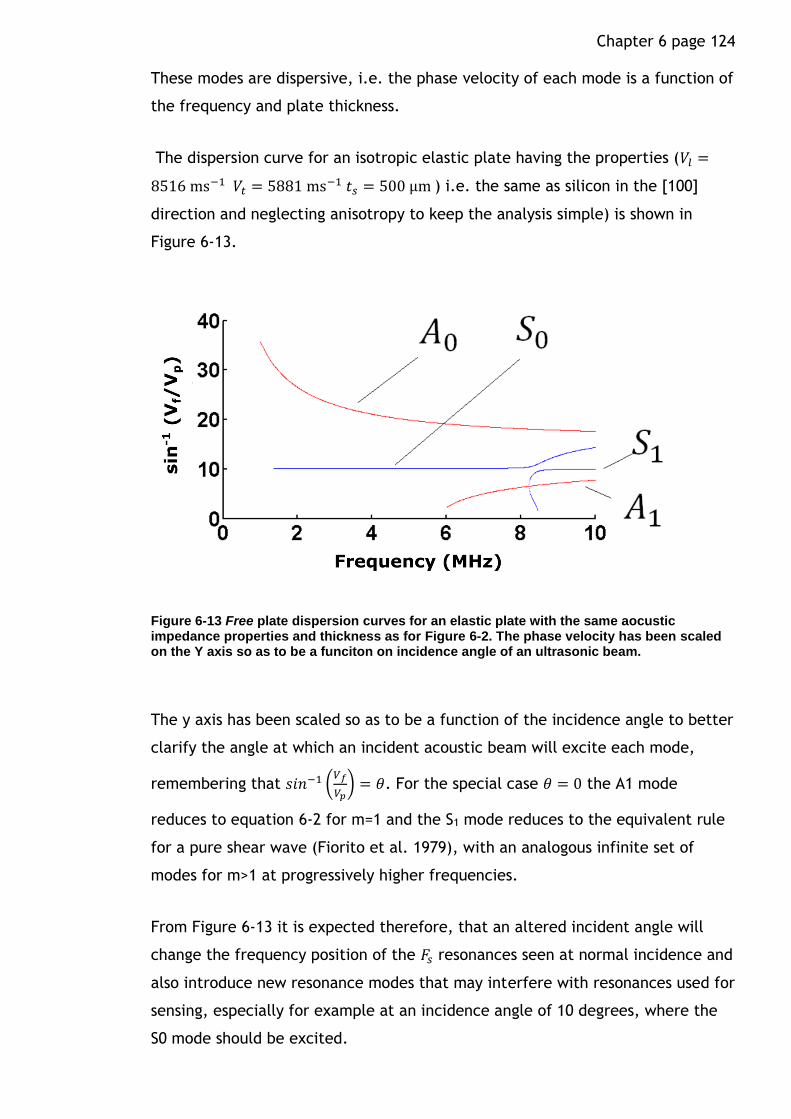
Chapter 6 page 124

These modes are dispersive, i.e. the phase velocity of each mode is a function of

the frequency and plate thickness.

The dispersion curve for an isotropic elastic plate having the properties (𝑉𝑙 =

8516 ms−1 𝑉𝑡 = 5881 ms−1 𝑡𝑠 = 500 μm ) i.e. the same as silicon in the [100]

direction and neglecting anisotropy to keep the analysis simple) is shown in

Figure 6-13.

Figure 6-13 Free plate dispersion curves for an elastic plate with the same aocustic impedance properties and thickness as for Figure 6-2. The phase velocity has been scaled on the Y axis so as to be a funciton on incidence angle of an ultrasonic beam.

The y axis has been scaled so as to be a function of the incidence angle to better

clarify the angle at which an incident acoustic beam will excite each mode,

remembering that 𝑠𝑖𝑛−1 (𝑉𝑓

𝑉𝑝) = 𝜃. For the special case 𝜃 = 0 the A1 mode

reduces to equation 6-2 for m=1 and the S1 mode reduces to the equivalent rule

for a pure shear wave (Fiorito et al. 1979), with an analogous infinite set of

modes for m>1 at progressively higher frequencies.

From Figure 6-13 it is expected therefore, that an altered incident angle will

change the frequency position of the 𝐹𝑠 resonances seen at normal incidence and

also introduce new resonance modes that may interfere with resonances used for

sensing, especially for example at an incidence angle of 10 degrees, where the

S0 mode should be excited.

Chapter 6 page 125

Exact analytical expressions exist for the transmission and reflection coefficients

of a single immersed elastic plate (Fiorito et al. 1979). An example of the

reflection coefficient as a function of frequency and incident angle is shown in

Figure 6-14 for the same elastic plate in as in Figure 6-13 using these equations.

Figure 6-14 Reflection coefficient from a single isotropic elastic plate immersed in a fluid with the same impedance properties as in Figure 6-13. The coupling of the Lamb waves modes shown in Figure 6-13 is clearly recognisable as dips in the reflection spectrum.

As would be expected the position of the reflection minima follow the dispersion

curves of Figure 6-13, with a wide variation in their widths. The 𝑆0 and 𝐴1 modes

for example are extremely sharp.

Attention is now turned to the reflection coefficient from a series of elastic

plates immersed in a fluid. The COMSOL(Comsol Inc n.d.) model described in the

materials and methods section was used to calculate the reflection coefficient

from an angled incident beam. Figure 6-15 shows the reflection coefficient as a

function of frequency and incidence angle for two isotropic elastic plates with

the same properties and arrangement as in Figure 6-2. The top graph shows a

coarse plot of the reflection coefficient up 𝜃 = 21°. The 𝐴0, 𝐴1 and 𝑆1 modes can

be clearly seen. The resonances due to the fluid layer are also visible, and are

also clearly a function of theta. These resemble resonance modes from a free

liquid layer (Fiorito et al. 1986).

Chapter 6 page 126

Since the 𝑆0 mode is very sharp, it is not well resolved in the top figure, to show

its influence on the fluid resonances a zoomed in region at around 𝜃 = 10° is

shown on the right hand graph. This shows the displacement of the fluid layer

resonances as the lamb wave mode approaches the fluid layers resonances.

Beyond 𝜃 = 21° it would be expected that there are no more Lamb wave modes

that can interfere with the fluid layer resonances, the fluid layer resonances

themselves might be expected to still exist, however the peaks become

progressively sharper and are much harder to resolve without a very fine

frequency sweep. The bottom figure shows the reflection spectrum for an

incidence angle of 24 degrees as an example.

Figure 6-15 Reflection coefficient from a 3 layer structure as in Figure 6-2 as a function of incidence angle and frequency. Top shows the modulus of the reflection coefficient up to 𝜽 = 𝟐𝟎°, the middle shows a finer sweep around 𝜽 = 𝟏𝟎. 𝟎𝟗° in order to properly resolve the

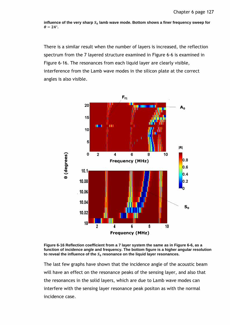
Chapter 6 page 127

influence of the very sharp 𝑺𝟎 lamb wave mode. Bottom shows a finer frequency sweep for 𝜽 = 𝟐𝟒°.

There is a similar result when the number of layers is increased, the reflection

spectrum from the 7 layered structure examined in Figure 6-6 is examined in

Figure 6-16. The resonances from each liquid layer are clearly visible,

interference from the Lamb wave modes in the silicon plate at the correct

angles is also visible.

Figure 6-16 Reflection coefficient from a 7 layer system the same as in Figure 6-6, as a function of incidence angle and frequency. The bottom figure is a higher angular resolution

to reveal the influence of the 𝑺𝟎 resonance on the liquid layer resonances.

The last few graphs have shown that the incidence angle of the acoustic beam

will have an effect on the resonance peaks of the sensing layer, and also that

the resonances in the solid layers, which are due to Lamb wave modes can

interfere with the sensing layer resonance peak positon as with the normal

incidence case.

Chapter 6 page 128

A problem to solve therefore is being able to properly distinguish between

changes in incidence angle and changes in the properties of the sensing layer. A

solution could be to include a reference system alongside the chemically

sensitive layer structure that could be used to first determine incidence angle.

The reference system could for example be another layered structure that is

insensitive to change in glucose concentration. The reflections from both of

these structures could be measured simultaneously by designing them such that

the resonances used for evaluation do not overlap.

6.4 Conclusions

This chapter has investigated how a layered structure of different materials

could be used as a remote sensing device, using ultrasonic waves to

communicate wirelessly with the device and a transducer. Using a layered stack

holds some promise because of the sharp transmission resonances that can be

generated and measured in the reflection spectrum. Changes in the frequency

positon of these resonances imply physical changes (thickness, sound speed) that

occur in one or more of the layers. The particular focus of this thesis is to

investigate how this physical system might be exploited as a subcutaneous

glucose sensor where the separation medium between the transducer and the

implant is the dermis. Since the dermis acts like another, albeit a very thick

layer in the system it has the potential to influence the measurement,

furthermore changes in the impedance or thickness of this layer would be

expected to change the position of the sensing layer resonances.

The impact of this depends on the required sensitivity of the device and also the

actual physical potential for changes in the separation medium over long period

of time. This seems quite likely, since even small, sub-millimetre changes in the

path-length (perhaps from movement of the implant or drying any couplant) can

be significant. However, it also depends on how the measurement is taken, if

this is simply measuring the position of the first mode resonance in the sensing

layer then there is certainly the potential for error in the measurement.

In this case, if the required sensitivity equated to measurement changes in the

frequency positon of the resonances to less than 1% the 3 layer structure

investigated in this chapter might not be sufficient. It has been shown in this

Chapter 6 page 129

chapter that adding more layers would greatly improve this, however it

increases the complexity.

Another potential problem is not just the movement of the implant, but

rotation, which will affect the angle of the layers relative to the beam. This will

also have influence the frequency positon of the sensing layer resonance. A

possible solution for this is to include a reference measurement from a static

layer structure where only the incidence angle could influence the positions of

one of its layer resonances.

An alternative to these measures might be to try and make use of the full

reflection spectrum rather than just monitoring the frequency position of one or

more resonance ‘peaks’. Authors working on problems falling under the Non-

destructive testing umbrella have used variations on an ‘inverse’ method to

deduce multiple properties from a measured reflection/transmission spectrum

by fitting it to a suitable model. For example (Yapura et al. 2004) were able to

infer all the thicknesses and impedances of a water immersed layered structure

consisting of 3 bonded metal layers, only needing to know the density of each

layer in advance. However for accurate results they needed to have a spectrum

wide enough to include at least 6 of the resonances.

This chapter has explored in some detail how ultrasonic waves might be used to

measure mechanical changes such as thickness, or acoustic impedance via

transmission resonances in a purposely design layered stack. In the next chapter

a way to make the link between a mechanical change and a chemical change is

examined by introducing a chemical sensitive hydrogel as one of the layers. This

link would open the way to the possible use of this structure as a chemical

sensor.

130

Chapter 7 A second step towards an ultrasonic glucose sensor

7.1 Introduction and Overview

The purpose of this chapter is to investigate whether the physical changes in a

glucose sensitive hydrogel could be measured using the ultrasonic reflection

spectrum from a system of layers with one of them being the hydrogel. There

are many different formulations in the literature on glucose sensitive hydrogels

that might be appropriate for incorporation into an acoustic sensor, in this

chapter a hydrogel which is known to contract as a function of glucose

concentration was investigated. A model system where the hydrogel layer was

replaced with a fluid layer was also investigated and compared with the

equivalent circuit model that was detailed in the previous chapter.

The hydrogel that was used in the experiments in this chapter followed the

formulation described in (Horgan et al. 2006), this is based on a polyacrylamide

hydrogel that has a derivative of boronic acid, 3-acrylamidophenylboronic acid

incorporated into it. This has been detailed in the materials and methods

chapter. There are many variations on this theme that have been proposed so

firstly a review of some of the different formulations is given.

Boronic acid as a glucose sensor

Boronic acid is a weak Lewis acid that can exist in aqueous solution in either an

uncharged trigonal state or a charged tetrahedral state (Cambre & Sumerlin

2011). The proportion existing in the charged tetrahedral form is dependent on

the pka of the boronic acid. It is known that boronic acids can bind with 1,2 and

1,3 cis-diols (for example glucose) reversibly through the formation of a boronic

acid diester (Lorand & Edwards 1959). The pka of the boronic acid diester is

usually lower than free boronic acid and can lead to an increased number of

charged boronate groups (James et al. 1996).

Chapter 7 page 131

Glucose sensing with boronic acid incorporated hydrogels

When a boronic acid moiety is incorporated into a hydrogel the reaction with

glucose can be exploited to produce swelling of the hydrogel due to the increase

of the Donnan potential (Ancla et al. 2011). This concept forms the basis of

many glucose sensing strategies, which monitor the volumetric changes of these

hydrogels to infer glucose concentration. Most of these use phenylboronic acid

containing moieties, where addition of various substituents on the phenyl ring

allows the pka to be tuned so that these polymers can be used at physiologically

relevant pH (Wiskur et al. 2001).

Apart from the 1:1 binding of 1 glucose molecule to 1 boronate, there is also the

possibility of 2:1 binding of one glucose to two boronic acid groups at the same

time, utilising both pairs of hydroxyl groups on the glucose molecule (Alexeev et

al. 2004) (Horgan et al. 2006) (Pan et al. 2008). Here the 2:1 binding mechanism

acts like an extra cross-link which causes shrinking of the hydrogel. This has the

unfortunate effect of making the swelling behaviour of most boronic acid based

hydrogels competitive between the 1:1 binding and 2:1 binding, where the

dominant binding mechanism depends on both the concentration of boronic acid

molecules and the glucose concentration. For polymers with high concentrations

of PBA or 5-amino-2-flurophenyloronic acid (5A 2FPBA) 2:1 binding was found to

be favoured in (Ben-Moshe et al. 2006). This has also been confirmed in a

systematic study investigating twenty chemically distinct phenybronoic acids

(Zhang et al. 2013). However it was found for phenybronoic acids exhibiting fast

response kinetics 2:1 binding was favoured at low glucose concentrations and 1:1

binding at high (and still physiologically relevant) glucose concentrations. This

was evident through swelling of the hydrogel. This non-linear behaviour is

obviously undesirable since it leads to the same hydrogel volume for two

different glucose concentrations.

An interesting strategy to overcome this used a volume resetting agent

incorporated into the hydrogel to pre-crosslink the hydrogel so that addition of

glucose could only lead to the formation of 1:1 bonds. PVA polymer chains were

used as the volume resetting agent, which contain 1,3 diols, these have lower

affinities for PBA than the 1,2 diols on glucose, so the glucose can displace the

Chapter 7 page 132

PVA and form 1:1 bonds. This resulted in a hydrogel with a linear relationship

with glucose up to 60 mmol L-1 with low hysteresis (Zhang et al. 2014).

Another problem is specificity for glucose, boronic acid can bind with other

molecules present in the body such as other types of sugar and lactate which

also produce swelling of the hydrogel. Fortunately glucose is the only saccharide

in the blood in significant quantities, the next two being fructose and galactose

with concentrations of less than 0.1 mmol L-1 (Kawasaki et al. 2004; Horgan et

al. 2006). However lacate is present in sufficient quantities in the blood to

affect the hydrogel swelling (Kabilan et al. 2005).

A solution which has been tried by various different authors is to incorporate a

cationic monomer into the hydrogel matrix (Alexeev et al. 2003) (Tierney et al.

2009) (Horgan et al. 2006). Introduction of (3-

acrylamidopropyl)trimethylammonium chloride (ATMA) as the cationic monomer

was found to eliminate the interference from lactate and other sachardies for

appropriate mol% mixtures of monomer constituents (Horgan et al. 2006). This is

hypothesised to work by charge neutralisation stabilisation, introduction of a

cationic monomer in close proximity to the boronate group stabilizes its charged

form, reducing the swelling effect of 1:1 binding. This favours the contracting

effect of 2:1 binding and since lactate, fructose and galactose do not have a pair

of cis-diols to undergo 2:1 binding the swelling effect of these molecules is

greatly reduced.

Glucose sensing polymer solutions using boronic acid

Other strategies have used boronic acid binding to change the viscosity of a

polymer solution, with the first reported in (Kitano et al. 1991). A contemporary

example of this strategy can be found in (Li et al. 2009) which used 3-

acrylamidophenylboronic acid incorporated into polyacrylamide chains dissolved

in phosphate buffer saline at Ph 7.4. The addition of glucose formed cross-links

between the polymer chains increasing the viscosity. This polymer solution has

been incorporated into an overall device proposed for subcutaneous continuous

glucose monitoring which uses a semi-permeable membrane to keep the polymer

chains contained within the device while allowing glucose to diffuse through the

membrane (Huang et al. 2013).

Chapter 7 page 133

Alternative glucose sensing molecules

Apart from boronic acid, concanavalin A (Miyataa et al. 1996) and glucose

oxidase (Holtz & Asher 1997) have also been investigated as molecular receptors

for mechanically changing a hydrogel/polymer solution. However while these

proteins are highly specific to glucose the potential for denaturation limits the

longevity of these sensors (Zahnley 1981) (Cambre & Sumerlin 2011). There are

also toxicity concerns with concanavalin A (Li et al. 2009).

A polyacrylamide hydrogel containing 3-APB and ATMA has been selected for this

study due to its demonstrated specificity for glucose (Horgan et al. 2006). This

hydrogel contracts with increasing glucose concentrations as more cross-links

(2:1 binding reaction) are created.

Ultrasonic characterisation of hydrogels

The acoustic properties of hydrogels have been studied by a number of authors,

which has useful insights for this study. They key points are briefly described in

this section.

Biot’s theory of acoustic wave propagation in poroelastic media has also been

applied to gels, for example see (Johnson 1982) (Chiarelli et al. 2010). Due to

the typically very small pores sizes of gels the theory can usually be applied at

its low frequency limit, i.e. the fast and shear wave modes will propagate,

however the slow wave is diffusive (see section on porosity in the last chapter).

Since hydrogels usually have very high water contents (80-90% w/w) the phase

velocity of the wave is usually close that of water.

Observations of acoustic wave velocity and attenuation for poly (2-hydroxyethyl

methacrylate)(HEMA) hydrogels undergoing water sorption has been reported in

(Maffezzoli et al. n.d.) in which the phase velocity is observed to decrease from

3300 ms-1 when dry to 1600 ms-1 when swollen. The attenuation was also

observed to be lower in the swollen state. Ultrasonic measurements on

poly(vinyl alcohol) (PVA) have also been reported in (Surry et al. 2004;

Fromageau et al. 2007). As the PVA hydrogel is put through successive freeze-

thaw cycles it becomes more cross-linked and the water content is reduced.

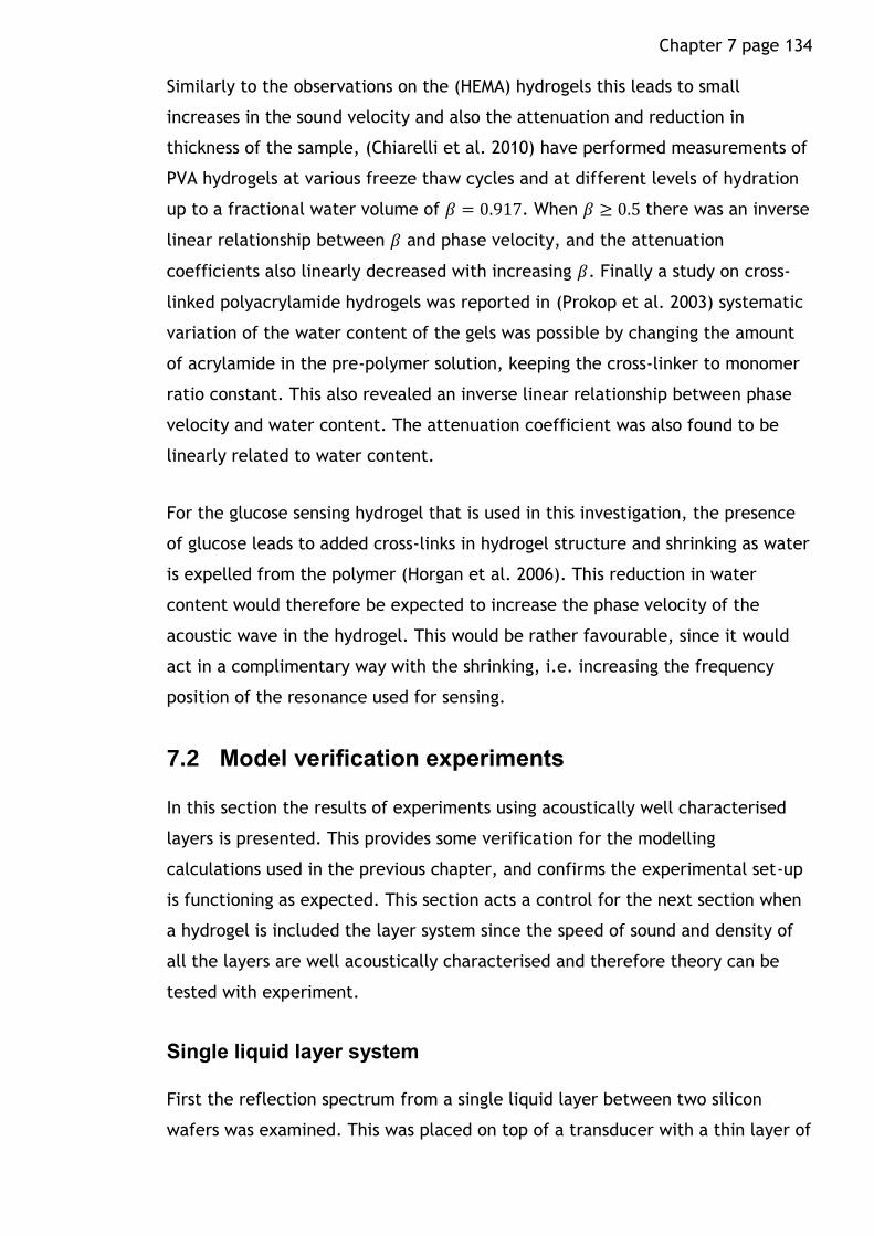
Chapter 7 page 134

Similarly to the observations on the (HEMA) hydrogels this leads to small

increases in the sound velocity and also the attenuation and reduction in

thickness of the sample, (Chiarelli et al. 2010) have performed measurements of

PVA hydrogels at various freeze thaw cycles and at different levels of hydration

up to a fractional water volume of 𝛽 = 0.917. When 𝛽 ≥ 0.5 there was an inverse

linear relationship between 𝛽 and phase velocity, and the attenuation

coefficients also linearly decreased with increasing 𝛽. Finally a study on cross-

linked polyacrylamide hydrogels was reported in (Prokop et al. 2003) systematic

variation of the water content of the gels was possible by changing the amount

of acrylamide in the pre-polymer solution, keeping the cross-linker to monomer

ratio constant. This also revealed an inverse linear relationship between phase

velocity and water content. The attenuation coefficient was also found to be

linearly related to water content.

For the glucose sensing hydrogel that is used in this investigation, the presence

of glucose leads to added cross-links in hydrogel structure and shrinking as water

is expelled from the polymer (Horgan et al. 2006). This reduction in water

content would therefore be expected to increase the phase velocity of the

acoustic wave in the hydrogel. This would be rather favourable, since it would

act in a complimentary way with the shrinking, i.e. increasing the frequency

position of the resonance used for sensing.

7.2 Model verification experiments

In this section the results of experiments using acoustically well characterised

layers is presented. This provides some verification for the modelling

calculations used in the previous chapter, and confirms the experimental set-up

is functioning as expected. This section acts a control for the next section when

a hydrogel is included the layer system since the speed of sound and density of

all the layers are well acoustically characterised and therefore theory can be

tested with experiment.

Single liquid layer system

First the reflection spectrum from a single liquid layer between two silicon

wafers was examined. This was placed on top of a transducer with a thin layer of

Chapter 7 page 135

water acting as a couplant layer between the silicon and the transducer face. It

was found through experimentation and simulation that the boundary conditions

at the top silicon surface (i.e. the reflectivity) and also the thickness of the

couplant layer could affect the positon of the resonance peaks so these had to

be controlled in the following way. Firstly a flow cell was created using PDMS so

that the impedance of the medium on the top surface of the silicon layer could

be controlled (i.e. as that of water) the PDMS roof also acted to damp most of

the transmitted wave and minimize reflections. This also allowed the fluid in the

layers to be changed without having to move the set-up, as different fluid

concentrations could be pumped through the flow cell. This helped to keep the

thickness of the couplant layer well controlled. A further precaution of waiting

for the position of the resonance peak to come to equilibrium before starting an

experiment also helped to minimize interference from the changes in thickness

of the couplant layer. The thickness of each layer has been listed in the table in

the appendix section of this chapter, measured with a micrometer. The wave

velocities in the silicon layers were the same as in the previous chapter and the

wave velocity in the water was determined by first noting the temperature and

using the velocity formulae found in (Millero 1978). The parameters for the

transducer were as stated in the materials and methods chapter. An illustration

has been placed to the left of the figures to show the sequential order of the

layers and the boundary conditions. The thickness of the couplant layer was

chosen so that there was the best fit with the data. In the experiment where the

fluid properties in the flow chamber were systematically changed by adding

different concentrations of NaCl, this was performed once at the start and kept

constant for the rest of the experiment.

An example of the reflection magnitude and group delay seen at the electric

signal input across the lead metaniobate transducer has been shown in Figure

7-1 along with the KLM model predictions and the simpler acoustic transmission

model that does not include the electrical part of the transducer.

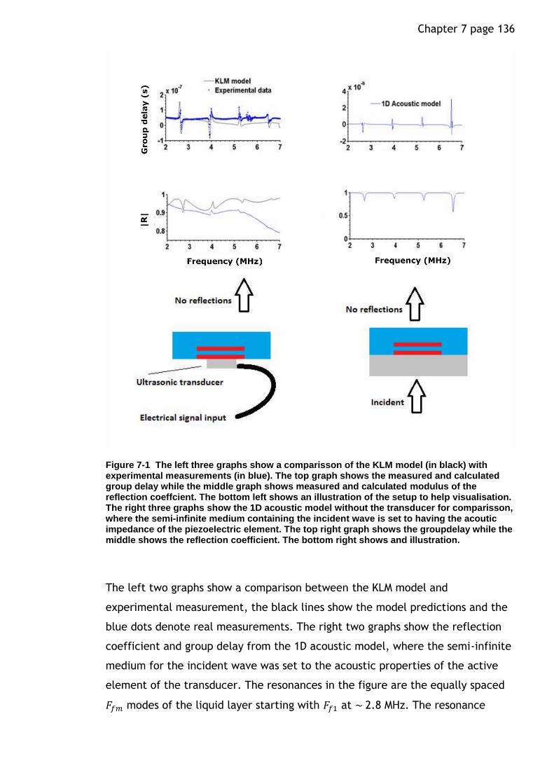
Chapter 7 page 136

Figure 7-1 The left three graphs show a comparisson of the KLM model (in black) with experimental measurements (in blue). The top graph shows the measured and calculated group delay while the middle graph shows measured and calculated modulus of the reflection coeffcient. The bottom left shows an illustration of the setup to help visualisation. The right three graphs show the 1D acoustic model without the transducer for comparisson, where the semi-infinite medium containing the incident wave is set to having the acoutic impedance of the piezoelectric element. The top right graph shows the groupdelay while the middle shows the reflection coefficient. The bottom right shows and illustration.

The left two graphs show a comparison between the KLM model and

experimental measurement, the black lines show the model predictions and the

blue dots denote real measurements. The right two graphs show the reflection

coefficient and group delay from the 1D acoustic model, where the semi-infinite

medium for the incident wave was set to the acoustic properties of the active

element of the transducer. The resonances in the figure are the equally spaced

𝐹𝑓𝑚 modes of the liquid layer starting with 𝐹𝑓1 at ~ 2.8 MHz. The resonance

Chapter 7 page 137

modes corresponding to the silicon plates start at about 8 MHz and so are not

within the range of the plotted spectrum.

Although both models correlate very well with the measured reflection and

group delay spectrum, and so either could be used to think about how a layered

system might be used as a sensor, the KLM model gives a more meaningful and

direct comparison with the experimental data, since it is the reflection of an

electrical wave that is being measured. The magnitude and shape of the dips

and peaks that show the position of the resonances is also predicted with more

accuracy. This is an interesting point since the simple acoustic model predicts

simple well behaved symmetric dips in the reflection spectrum, what is actually

seen is more complex than this due to the coupling of the acoustic and electrical

parts of the system.

For example, it can be seen from the reflection coefficient at the transducer

that the resonances are superimposed on-top of the reflection spectrum of the

transducer and its quarter wave-matching layer. The centre frequency of the

bandwidth for the transducer used in this experiment was 3.5 MHz and it can be

seen that further from the bandwidth the magnitude of the resonances becomes

smaller, as would be expected since less of the electric signal is converted to an

acoustic wave and hence less energy is transmitted through the layer structure.

The difference in the slope of the reflection magnitude between the KLM model

and the experimental measurements suggests a frequency dependent loss

mechanism in the transducer, possibly from the matching network or losses in

the cable. This slope is also evident when there are no layers in front of the

transducer, so it is not a loss mechanism due the acoustic reflections.

Since the resonances of interest have much sharper gradients than the

background slope of the transducer reflections, differentiating the reflection or

phase spectrum with respect to frequency can help to remove some of the

background slope. This can be seen in the group delay plots on the right hand

side of Figure 7-1, with a similar looking plot for the gradient of the magnitude

of the reflection coefficient.

Chapter 7 page 138

The group delay spectrum for a liquid layer gap of 3452 μm and 5502 μm is

shown in Figure 7-2. The top two graphs show the experimental measurements

and below shows the predictions from the KLM model.

Figure 7-2 (Top left and right) Measured group delay for a 345 and 550 μm liquid layer thickness. (Bottom left and right) modelled group delay for a 345 and 550 μm liquid layer thickness.

All these resonances again correspond with the 𝐹𝑓𝑚 modes of the liquid layer.

Again there is very good correlative agreement with the model, with the

exception of the observed peak at ~5.5 MHz which is not predicted in the model.

This peak was observed to also be present with only a single silicon wafer on the

transducer and is probably due some of the energy in the transducer being

converted to a shear wave.

By adding different concentrations of sodium chloride the speed of sound in the

fluid layer could be systematically altered (see materials and methods chapter).

Figure 7-3 shows an example of the position of the 𝐹𝑓2 resonance in the 345 μm

liquid gap structure at just above 4 MHz over time as the concentration of the

sodium chloride was increased. The vertical lines show the time point at which a

new concentration of sodium chloride was introduced, (see materials and

methods chapter).

Chapter 7 page 139

Figure 7-3 Position of the 𝑭𝒇𝟐for the 345 μm liquid layer gap as the concentration of sodium

chloride is systematically increased. The vertical lines show the time point when a new salt concentration was introduced. The insert shows the position of the resonance peak at equilibrium for each concentration against the KLM model predictions.

The position of the resonance was determined by taking the absolute value of

the differential of the group delay spectrum to remove the background slope of

the signal. Lower and upper and half-maximum positons were then determined

for the peak, the average positon between these two points was taken as the

measurement. The errorbars were set as the width of the resonance at half-

maximum.

A small difference of ~15-30 kHz is evident between the measurement and the

KLM model predictions. However this is within the measurement error for the

thickness of the layers (2 μm). The total change in the fluid sound velocity over

this range was 3.14%. Considering a minimum detectable change to be the half-

maximum width of the resonance, the accuracy of this method can be estimated

as that needed to change the frequency positon by that much. The minimum

sound velocity change would then be ±10 ms-1, ~0.6% of the velocity of DI water.

The linear relationship in Figure 7-3 is what would be expected from using the

rule of thumb discussed in the previous chapter for resonances at oblique

incidence angle, so long as the resonance is far enough away from other

resonances in the spectrum. This has not been plotted on the insert in Figure

7-3, however it gives an identical gradient as the KLM model prediction, however

shifted down significantly.

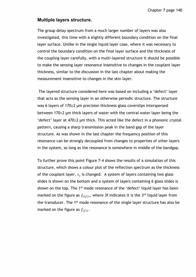
Chapter 7 page 140

Multiple layers structure.

The group delay spectrum from a much larger number of layers was also

investigated, this time with a slightly different boundary condition on the final

layer surface. Unlike in the single liquid layer case, where it was necessary to

control the boundary condition on the final layer surface and the thickness of

the coupling layer carefully, with a multi-layered structure it should be possible

to make the sensing layer resonance insensitive to changes in the couplant layer

thickness, similar to the discussion in the last chapter about making the

measurement insensitive to changes in the skin layer.

The layered structure considered here was based on including a ‘defect’ layer

that acts as the sensing layer in an otherwise periodic structure. The structure

was 6 layers of 1702 μm precision thickness glass coverslips interspersed

between 1702 μm thick layers of water with the central water layer being the

‘defect’ layer at 4702 μm thick. This acted like the defect in a phononic crystal

pattern, causing a sharp transmission peak in the band gap of the layer

structure. As was shown in the last chapter the frequency position of this

resonance can be strongly decoupled from changes to properties of other layers

in the system, so long as the resonance is somewhere in middle of the bandgap.

To further prove this point Figure 7-4 shows the results of a simulation of this

structure, which shows a colour plot of the reflection spectrum as the thickness

of the couplant layer, 𝑡𝑐 is changed. A system of layers containing two glass

slides is shown on the bottom and a system of layers containing 6 glass slides is

shown on the top. The 1st mode resonance of the ‘defect’ liquid layer has been

marked on the figure as 𝑓(3𝑓)1, where 3f indicates it is the 3rd liquid layer from

the transducer. The 1st mode resonance of the single layer structure has also be

marked on the figure as 𝑓(𝑓)1.

Chapter 7 page 141

Figure 7-4 KLM simulation of Group delay spectrum as a function of couplant layer thickness for 1 liquid layer system, (bottom) and 6 liquid layer system as described in the text. (top)

Over a range of 0 to 50 μm couplant thickness, there is a 1 kHz shift in the

position of the 𝑓(3𝑓)1 resonance from the 6 layer structure however there is a

change of 325 kHz in the single liquid layer structure.

Since with a six layer structure the couplant thickness does not have to be

controlled so rigorously, it is possible to monitor the changes in the sensing layer

without the need for controlling the thickness of the couplant layer or the

impedance of the final (non reflecting) layer. This allows for a much simpler

experimental set-up without the need for a flow chamber. A typical reflection

spectrum measurement and simulation prediction for this structure are shown in

Figure 7-5.

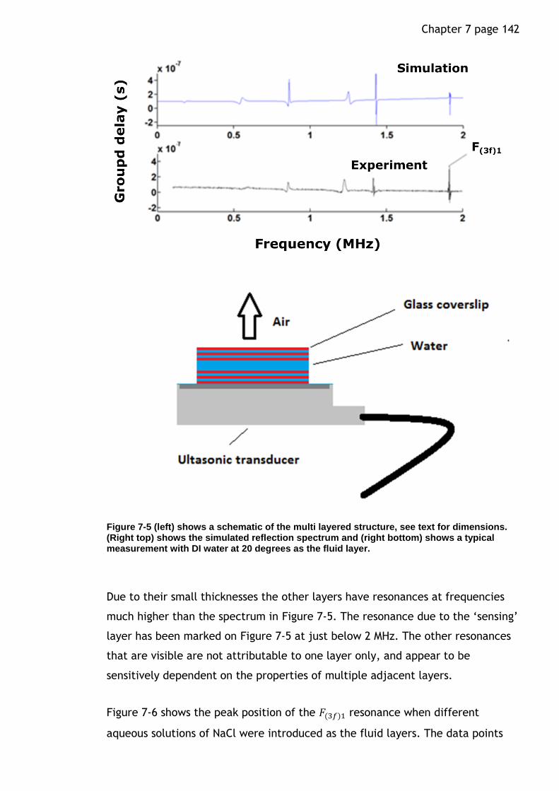
Chapter 7 page 142

Figure 7-5 (left) shows a schematic of the multi layered structure, see text for dimensions. (Right top) shows the simulated reflection spectrum and (right bottom) shows a typical measurement with DI water at 20 degrees as the fluid layer.

Due to their small thicknesses the other layers have resonances at frequencies

much higher than the spectrum in Figure 7-5. The resonance due to the ‘sensing’

layer has been marked on Figure 7-5 at just below 2 MHz. The other resonances

that are visible are not attributable to one layer only, and appear to be

sensitively dependent on the properties of multiple adjacent layers.

Figure 7-6 shows the peak position of the 𝐹(3𝑓)1 resonance when different

aqueous solutions of NaCl were introduced as the fluid layers. The data points

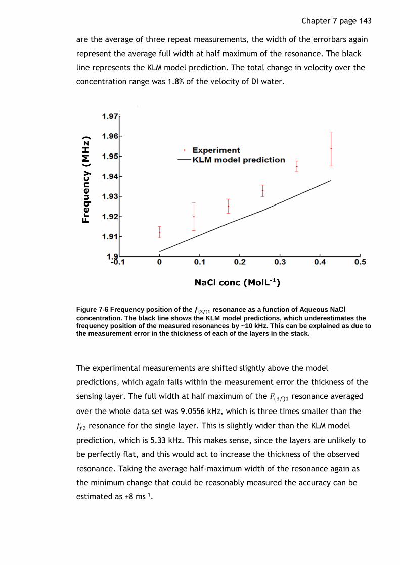
Chapter 7 page 143

are the average of three repeat measurements, the width of the errorbars again

represent the average full width at half maximum of the resonance. The black

line represents the KLM model prediction. The total change in velocity over the

concentration range was 1.8% of the velocity of DI water.

Figure 7-6 Frequency position of the 𝒇(𝟑𝒇)𝟏 resonance as a function of Aqueous NaCl

concentration. The black line shows the KLM model predictions, which underestimates the frequency position of the measured resonances by ~10 kHz. This can be explained as due to the measurement error in the thickness of each of the layers in the stack.

The experimental measurements are shifted slightly above the model

predictions, which again falls within the measurement error the thickness of the

sensing layer. The full width at half maximum of the 𝐹(3𝑓)1 resonance averaged

over the whole data set was 9.0556 kHz, which is three times smaller than the

𝑓𝑓2 resonance for the single layer. This is slightly wider than the KLM model

prediction, which is 5.33 kHz. This makes sense, since the layers are unlikely to

be perfectly flat, and this would act to increase the thickness of the observed

resonance. Taking the average half-maximum width of the resonance again as

the minimum change that could be reasonably measured the accuracy can be

estimated as ±8 ms-1.

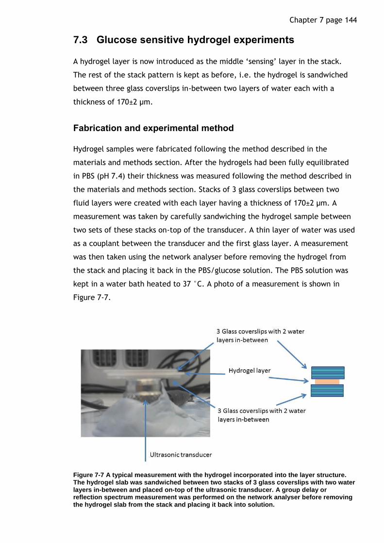
Chapter 7 page 144

7.3 Glucose sensitive hydrogel experiments

A hydrogel layer is now introduced as the middle ‘sensing’ layer in the stack.

The rest of the stack pattern is kept as before, i.e. the hydrogel is sandwiched

between three glass coverslips in-between two layers of water each with a

thickness of 170±2 µm.

Fabrication and experimental method

Hydrogel samples were fabricated following the method described in the

materials and methods section. After the hydrogels had been fully equilibrated

in PBS (pH 7.4) their thickness was measured following the method described in

the materials and methods section. Stacks of 3 glass coverslips between two

fluid layers were created with each layer having a thickness of 170±2 μm. A

measurement was taken by carefully sandwiching the hydrogel sample between

two sets of these stacks on-top of the transducer. A thin layer of water was used

as a couplant between the transducer and the first glass layer. A measurement

was then taken using the network analyser before removing the hydrogel from

the stack and placing it back in the PBS/glucose solution. The PBS solution was

kept in a water bath heated to 37 °C. A photo of a measurement is shown in

Figure 7-7.

Figure 7-7 A typical measurement with the hydrogel incorporated into the layer structure. The hydrogel slab was sandwiched between two stacks of 3 glass coverslips with two water layers in-between and placed on-top of the ultrasonic transducer. A group delay or reflection spectrum measurement was performed on the network analyser before removing the hydrogel slab from the stack and placing it back into solution.

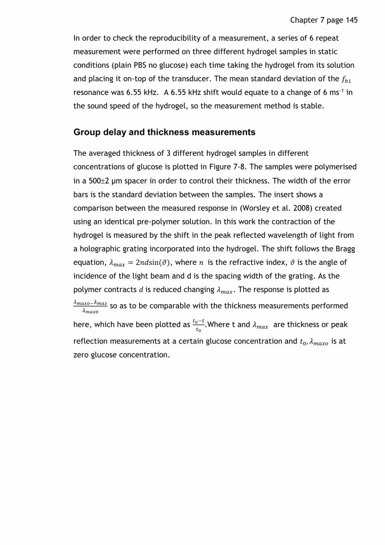
Chapter 7 page 145

In order to check the reproducibility of a measurement, a series of 6 repeat

measurement were performed on three different hydrogel samples in static

conditions (plain PBS no glucose) each time taking the hydrogel from its solution

and placing it on-top of the transducer. The mean standard deviation of the 𝑓ℎ1

resonance was 6.55 kHz. A 6.55 kHz shift would equate to a change of 6 ms-1 in

the sound speed of the hydrogel, so the measurement method is stable.

Group delay and thickness measurements

The averaged thickness of 3 different hydrogel samples in different

concentrations of glucose is plotted in Figure 7-8. The samples were polymerised

in a 5002 μm spacer in order to control their thickness. The width of the error

bars is the standard deviation between the samples. The insert shows a

comparison between the measured response in (Worsley et al. 2008) created

using an identical pre-polymer solution. In this work the contraction of the

hydrogel is measured by the shift in the peak reflected wavelength of light from

a holographic grating incorporated into the hydrogel. The shift follows the Bragg

equation, 𝜆𝑚𝑎𝑥 = 2𝑛𝑑sin(𝜗), where 𝑛 is the refractive index, 𝜗 is the angle of

incidence of the light beam and d is the spacing width of the grating. As the

polymer contracts 𝑑 is reduced changing 𝜆𝑚𝑎𝑥. The response is plotted as

𝜆𝑚𝑎𝑥𝑜−𝜆𝑚𝑎𝑥

𝜆𝑚𝑎𝑥0 so as to be comparable with the thickness measurements performed

here, which have been plotted as 𝑡0−𝑡

𝑡0.Where t and 𝜆𝑚𝑎𝑥 are thickness or peak

reflection measurements at a certain glucose concentration and 𝑡0, 𝜆𝑚𝑎𝑥𝑜 is at

zero glucose concentration.

Chapter 7 page 146

Figure 7-8 (Main figure) Average thickness of 3 hydrogel samples initially polymerised in a

500 2 μm thick cavity between two glass coverslips. The error bars are the standard deviation of the thicknesses of the hydrogel samples. (Insert) Response of hydrogel samples (red dots) compared with measurements from (Worsley et al. 2008) (blue squares) where an identical hydrogel pre-polymer solution was used.

After polymerisation and replacement of the DMSO solvent with PBS the

thickness of the hydrogel swells by ~ 50% from the initial 500 μm. The

diminishing thickness change with increasing concentration of glucose is in

reasonable agreement with observations made by other workers using the same

polymer formulation (Horgan et al. 2006) (Worsley et al. 2008), which as

previously indicated, is due to the increased number of cross-links between

different boronate groups as they bind with glucose. A similar inverse power law

relationship between swelling and cross-link density has been observed for

polyacrylamide hydrogels copolymerised with another cationic monomer,

[(methacrylamido)propyl]trimethylammonium chloride (MAPTAC) in aqueous salt

concentrations (Hooper et al. 1990). The comparison in the insert has to be

taken carefully as there is an assumption that the measured response reported in

(Worsley et al. 2008) is only dependent on the distance between the light

scatterers and not the refractive index change of the hydrogel. However

refractive index change is not expected to have a large effect of the

measurement (Horgan et al. 2006). This comparison provides reasonably good

evidence that the hydrogel samples were fabricated correctly and functioning as

expected.

Chapter 7 page 147

Group delay measurements

By combining the ultrasonic group delay spectrum measurement with thickness

measurements of the hydrogel the sound speed in the hydrogel could be inferred

by adjusting the polymer sound velocity parameters in the KLM model, all other

parameters describing the layers in the stack being fixed by measurement.

Measurement uncertainty was estimated by matching the velocity of the

hydrogel when the thicknesses of the other layers were increased or decreased

by the measurement tolerance of each layer.

An example of a measured group delay spectrum compared with a fitted

simulation prediction is shown in Figure 7-9 for a 706±7.5 μm thick hydrogel

sample in plain PBS solution at 37°C. The first 4 resonance modes for the

hydrogel layer have been marked on the figure. The 1𝑠𝑡 mode resonances of the

170 μm thick water layers are situated in the region between 4.5 and 5 MHz.

Figure 7-9 (Top) Example of a typical measured group delay spectrum with a hydrogel layer introduced as the sensing layer. (Bottom) KLM simulation where the phase velocity of the hydrogel layer in the simulation has been fitted so that the frequeny positon of the resonances agree with experiment. The fitted sound velocity was 1548± 12 ms-1.

Chapter 7 page 148

Sound velocity fitting

The fitted sound velocity was 1548±12 ms-1, this is a sensible value, considering

the proportion of water in the hydrogel. The weight fraction of the polymer

monomers to DMSO in the pre-polymer solution was 34%, furthermore upon

polymerisation and hydration the hydrogel swelled significantly as the water

replaces DMSO in the hydrogel, increasing the weight fraction of the solvent still

further (see Figure 7-8). It is therefore not surprising that the sound velocity in

the hydrogel is close to that of water. Sound velocity measurements of

Polyacrylamide hydrogel have also been performed in (Prokop et al. 2003), with

very similar results (for hydrogels with 81% w/w the speed was measured as

1568±2 ms-1).

Effect of glucose addition on resonance position

In Figure 7-10 the frequency positon of the 𝑓ℎ1 resonance for hydrogel samples

that have come to equilibrium in PBS solutions containing different

concentrations of glucose is plotted. The hydrogel samples were initially

polymerised in a 500 μm thick cavity. Each data point is the average of two

different samples and the error bars are the width of the standard deviation.

Chapter 7 page 149

Figure 7-10 Frequency position of 𝒇𝒉𝟏resonance as a function of glucose concentration in

PBS soluiton (Ph 7.4) at 𝟑𝟕 ℃. Each data point is the average measured position of 2 different hydrogel samples. Each samples was left overnight to come to equilibrium.

In contrast to the thickness measurements and the measurements from other

researchers (Horgan et al. 2006; Worsley et al. 2008) (see Figure 7-8) the

resonance position as a function of frequency is almost linear up to 10 mmol L-1.

This change in the frequency positon of the 𝑓ℎ1 resonance cannot be accounted

for by the thickness changes in the hydrogel alone, which would predict the

resonance position at 10 mmol L-1 glucose concentration as being 1.701 MHz.

This implies there is also a change in the sound speed of the hydrogel. Density

changes (not counting the effect it has on the hydrogel sound velocity) can be

ignored since the density difference between water and the hydrogel chains is

very small, and this has a negligibly small effect on the frequency position of the

resonance. For example in (Prokop et al. 2003) changing the water content of a

polyacrylamide hydrogel from 87 to 76% resulted in a 2.73% change in the

density, which only amounts to a change of 5 kHz in the frequency position of

the 𝑓ℎ1 resonance.

Using the averaged thickness of the hydrogel samples in Figure 7-8 at 10 mmol L-

1 the sound velocity in the hydrogel at 10 mmol L-1 was inferred as 1582± 12 ms-

Chapter 7 page 150

1, which is an increase of 34 ms-1 on the zero glucose velocity. This makes good

sense considering the changes that are expected to be happening inside the

hydrogel as the glucose concentration is increased from 0-10 mmol L-1. As new

crosslinks are formed between the glucose and boronate groups the elastic

resistance to swelling increases and some of the water is expelled from the

hydrogel. This has the effect of increasing the speed of sound since the effective

elasticity of the hydrogel increases due to the reduction in water content.

Response of hydrogel over time

In order to measure the response of the hydrogel samples to a change in ambient

glucose concentration the group delay of the samples was measured over time. A

reference measurement was first made in PBS (pH 7.4) containing no glucose at

37 ℃. The samples were then placed in a 50 ml PBS solution and 10 mmol L-1 α-

D-glucose was added immediately before the hydrogels were inserted. The

frequency position of the 𝑓ℎ1 resonance was measured at short time intervals

until the hydrogel had come to equilibrium. The samples were then left over

night and checked in the morning to ensure that they had fully come to

equilibrium. The samples were then placed back in zero glucose PBS and the

frequency position of the 𝑓ℎ1 resonance was measured at short time intervals

until it had stopped changing once again. This step was repeated for glucose

concentrations of 5 and 2.5 mmol L-1.

The change in the frequency position of the 𝑓ℎ1 resonance has been plotted in

Figure 7-11 for different changes in the glucose concentration. The left-hand

graph shows the measured response due to stated increases in glucose

concentration and the right hand shows the response to decreases. Each data

point is the average of two samples and the error-bars are the standard

deviation.

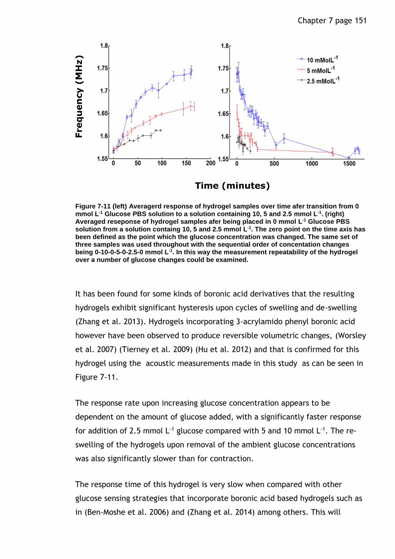
Chapter 7 page 151

Figure 7-11 (left) Averagerd response of hydrogel samples over time afer transition from 0 mmol L-1 Glucose PBS solution to a solution containing 10, 5 and 2.5 mmol L-1. (right) Averaged reseponse of hydrogel samples afer being placed in 0 mmol L-1 Glucose PBS solution from a solution containg 10, 5 and 2.5 mmol L-1. The zero point on the time axis has been defined as the point which the glucose concentration was changed. The same set of three samples was used throughout with the sequential order of concentation changes being 0-10-0-5-0-2.5-0 mmol L-1. In this way the measurement repeatability of the hydrogel over a number of glucose changes could be examined.

It has been found for some kinds of boronic acid derivatives that the resulting

hydrogels exhibit significant hysteresis upon cycles of swelling and de-swelling

(Zhang et al. 2013). Hydrogels incorporating 3-acrylamido phenyl boronic acid

however have been observed to produce reversible volumetric changes, (Worsley

et al. 2007) (Tierney et al. 2009) (Hu et al. 2012) and that is confirmed for this

hydrogel using the acoustic measurements made in this study as can be seen in

Figure 7-11.

The response rate upon increasing glucose concentration appears to be

dependent on the amount of glucose added, with a significantly faster response

for addition of 2.5 mmol L-1 glucose compared with 5 and 10 mmol L-1. The re-

swelling of the hydrogels upon removal of the ambient glucose concentrations

was also significantly slower than for contraction.

The response time of this hydrogel is very slow when compared with other

glucose sensing strategies that incorporate boronic acid based hydrogels such as

in (Ben-Moshe et al. 2006) and (Zhang et al. 2014) among others. This will

Chapter 7 page 152

undoubtedly be partly due to the large thickness of the hydrogels slabs which

were ~ 700 μm thick.

The diffusion coefficient of glucose through a similar hydrogel configuration

without a cationic monomer, ( i.e. acrylamide, MBA, 5 amino-2-

fluorophenylboronic acid) has been measured as similar to diffusion in water

~3x10-6 cm2 s-1, (Ben-Moshe et al. 2006), which makes intuitive sense since

hydrogels are mainly water, this indicates that it is not diffusion of glucose that

forms the rate limiting factor (since for the hydrogel considered here

𝑡𝑑~𝑥2

2𝐷~337.5s). However, once the change in the number of cross-links has

occurred the hydrogel has to swell or contract. This requires the passage of

water molecules into or out of the hydrogel. A possibility is that a hydrophilic

polymer chain matrix creates a resistance to the passage of water through the

hydrogel which in turn effectively limits the response rate. Obviously making the

hydrogel thinner will increase the response rate. Another way might be to

incorporate hydrophobic units into the polymer chains. This is has been tried

with (n-hexyl acrylate) which increased the swelling kinetics by 2-3 times

depending on the amount of (n-hexyl acrylate) that was added. (Ben-Moshe et

al. 2006)

7.4 Conclusion

An acoustic method for measuring the volumetric changes in a glucose sensitive

hydrogel has been presented. The changes in frequency positon of the hydrogel

layer for physiologically relevant glucose concentrations were large enough to be

accurately monitored with this method. This was mainly due to the contraction

of the hydrogel although a small change in the sound speed of the hydrogel also

contributed to the measured change. The ISO 15197 accuracy standards for a

self-monitoring blood glucose device are currently that a measurement must be

within ±15% of reference glucose levels ≥ 5.55 mmol L-1 and within ± 0.83 mmol

L-1 for reference glucose levels ≤ 5.55 mmol L-1. (Aggidis et al. 2015) In the case

of this hydrogel, the technique is clearly capable of measuring glucose

concentration to within the required accuracy.

Chapter 7 page 153

The response time of the hydrogel was clearly far too slow. This is undoubtedly

partly due to the large thickness of the hydrogel used here. The large thickness

was required so that the hydrogel had enough mechanical strength to bear the

constant stacking and unstacking between the glass layers required for each

measurement. The intended next step is to make these layers porous so that

glucose can diffuse through the layers, enabling a permeant structure to be

made. The hydrogel layer could then be made to be much thinner. A limitation

on the layers thicknesses might then be due to the required ultrasonic

frequencies. As the layers get thinner, the resonance modes will move to higher

frequencies and there will be a point when the attenuation of the ultrasonic

signal through the skin and in the implant becomes too large to detect the

reflected signal. The ultrasonic attenuation of human skin is between 2-3.1

dBcm-1 MHz-1 varying between subjects based on age and sex. (Guittet et al.

1999). The ultrasonic attenuation of a polyacrylamide hydrogel depends on the

w/w of acrylamide to water and also temperature. It is much less than the

attenuation due to the skin, at 37 °C in a 15% acrylamide gel the attenuation of a

5 MHz ultrasonic wave was measured as 0.4 dB cm-1. It should be realistic then

to reduce the thickness of the layers to a least 100 µm where the cavity mode

frequency would be around 7.5 MHz, which would equate to a round trip

attenuation due to the skin of approximately 10 dB.

The hydrogel studied in this work changes its volumetric properties due to

changes in the elasticity of the hydrogel brought about by crosslinking. Changes

in the ambient pressure might be expected to also have an effect on the

contraction and swelling behaviour of the hydrogel. This could take the form of

periodic/temporal applications of pressure due to local muscle contraction,

exercise, sleeping on or knocking the implant etc, or it could take the form of

slowly varying mechanical forces due to the foreign body response or migration

of the implant. For example the collagen matrix that forms around an implant

can generate contractile forces that are enough to rupture breast implants and

bend and fracture subcutaneously implanted polystyrene discs. (Helton et al.

2011)

A way around this problem could be simply to add more reference parts to the

implant. In the previous chapter the idea of placing a reference layer system

Chapter 7 page 154

that is insensitive to glucose was suggested as a way of inferring incidence angle.

A similar stack could be applied to infer the mechanical pressure on the implant,

then a measurement would involve a two-step calibration process based on first

inferring incidence angle from a reference stack that is insensitive to mechanical

pressure and glucose concentration. Then the ambient mechanical is inferred

pressure based on a stack which possibly would contain the same hydrogel

without the glucose sensing molecule, 3-acrylamidophenylbornic acid.

𝜃FF

155

Chapter 8 Wider perspectives and future work

8.1 Further steps towards an in vivo acoustic glucose sensor

The work presented in the last two chapters demonstrates the plausibility of this

method for in-vivo sensing, however the practical details of how such a system

could be built have not yet been fully realised. The most important missing

component is the appropriate selection of a porous material that can act as the

high acoustic impedance layer from the acoustic point of view, and also allow

the timely diffusion of an analyte through to the sensing layer from the sensing

point of view. The requirements on this material are quite stringent, it must

have a very high acoustic impedance to ensure sharp resonances, and yet it must

also be porous enough to allow fast mass transport. These two features

contradict each other, and make selection of an appropriate porous material non

trivial. One possibility might be electrochemically etched silicon wafers, which

have cylindrical pores with a typical diameter between 10-100 nm. (Bustillo et

al. 2014) Silicon would be a good choice because of its high acoustic impedance,

and ease of manipulation using MEMs fabrication technology.

Using a contractible hydrogel as the sensing layer may not, with hindsight have

been the best choice, partly because of the slow response kinetics but also

because of the potential problems that would be encountered due to fluctuating

ambient mechanical pressure on the implant due to daily life. A much better

strategy might be to look at a glucose sensitive layer that changes its sound

speed upon glucose concentration rather than its thickness, allowing the

thickness of the layer to be rigidly controlled. For example the glucose sensing

fluid described in (Li et al. 2009) could be a much better choice. This also uses

3-acrylamidophenylboronic acid incorporated into polyacrylamide chains,

however this time the chains are not cross-linked together and will dissolve in

PBs at physiologically relevant pH. Addition of glucose again causes cross-links to

form between the boronic acids, which increases the viscosity of the fluid. This

has been incorporated into a MEMs fabricated viscosity sensor, which utilises a

porous membrane that traps the polymer chains inside the sensing region and

allows diffusion of glucose molecules through the membrane. It is reasonable to

Chapter 8 page 156

hypothesize that the speed of sound will be a function of the number of cross-

links, since this has been observed for other cross-linking solutions such as

cellulose (Lionetto et al. 2005). The question would be whether the change in

sound speed with number of crosslinks would be large enough to sense changes

physiologically relevant glucose concentrations.

8.2 Acoustic Bragg-stacks as sensors in general

Apart from the implantable glucose sensing concept explored in the last two

chapters, there might be potential for alternative sensing applications using the

idea of an acoustic Bragg cell which is ‘read’ remotely by a transducer. A

particularly attractive feature of this is the separation of the transducer and the

sensing structure. This could perhaps lead to applications for sensing in

environments that are hard to reach, such as in pipes or bioreactors or on the

seabed for example.

Another possibility might be in chemical sensing for diagnostic and biological

technology, where the ability to separate the wet chemistry from the

transducer/resonator could be advantageous as it allows a cheap disposable

sensing part while preserving the transducer which could be reused many times,

unlike thickness shear mode resonators or SAW wave sensors for example.

Incidentally, shear mode resonators are well known as being highly sensitive to

changes in mass on the surface of the crystal, and can detect surface binding of

proteins and cells (Kaspar et al. 2000). This is in fact governed by the same

equation as the rule of thumb equations seen in chapter 6, i.e. 𝑓 =𝑣

2𝑑 where v is

the sound speed of the crystal resonator and d is the thickness. When a layer of

molecules bind to the surface, they change the thickness, which in turn changes

the resonant frequency. The reason for the extreme sensitivity is the high

quality factor of the resonance, i.e. extremely sharp resonance peaks which

allow minute changes in resonant frequency to be resolved. Longitudinal bulk

resonators have the disadvantage of coupling into the fluid sample, which

lessons the Q factor. On the other hand the use of a layered acoustic material

makes a sensitive longitudinal wave chemical sensor more plausible since this

sharpens the resonance. Then even with the damping effect of a fluid it could be

possible to measure nm scale thickness changes in a layer. Figure 8-1 shows the

Chapter 8 page 157

group delay from different layered stacks where the thickness of the middle

layer is changed by 10 nm (from 12 to 12.01 µm) for a 3 and 11 layered stack.

Adding more layers continuous to sharpen the resonances and improve the

sensitivity further.

Figure 8-1 An example of an acoustic layer arrangement that could sense thickness changes of ~ 10 nm. In the illustration the red layers are high acoustic impedance (Z=19 MRayl) and the blue layers and low acoustic (1.5 MRayl) the grey region represents a broad bandwidth thickness mode transducer that has a central frequency of 75 MHz. The left graph shows the group delay around the 1st mode resonance for a 3 layers structure as shown on the illustration beneath when the middle layer is 12 and 12.01 µm. It is clear that the width of the resonance is far too wide to resolve the frequency shift. The right graph shows the group delay around the 1st mode resonance of an 11 layer stack. The resonance is sharp enough here to just resolve a thickness change of 10 nm.

158

8.3 PDMS tunnel concept

An interesting feature of the SAW streaming work that was described in this

thesis is the PDMS tunnels, which were used to spatially filter the SAW beam.

This allows a fine degree of control of the streaming flows inside the flow

chamber by careful positioning of the tunnel. This may have interesting

applications, for example creating flow vortices to trap particles against a

sheath flow. SAW waves have also been used to drive heating of samples for

PCR, and it might be interesting if it were possible to spatially pinpoint the SAW

heating effect and possible heat multiple samples at the same time.

8.4 SAW streaming in microfluidic channels

Alternatives to PDMS

PDMS is an attractive material to create microchannel networks because of its

relative ease of fabrication, transparency and convenient bonding properties.

This is true for research laboratories, but there are problems for use in

commercialised products because high throughput methods of manufacture such

as injection molding, rolling or embossing are not possible with PDMS (Sackmann

et al. 2014). Higher rigidity materials such as thermoplastics can be used, and in

the past etched silicon and glass have also be investigated. These materials have

a much higher rigidity, and it would be interesting how this affects the scale

dependency of SAW streaming. A pressure wave generated in a fluid in a silicon

or glass channel would strongly scatter off the walls of the channel. The

streaming body force would then be the superposition of the reflected waves

and the original refracted SAW beam. It is possible that efficient streaming could

then driven at lower frequencies as less of the beam energy is lost due to

refraction out of the fluid volume.

SAW induced boundary streaming

Apart from the bulk Eckart streaming, SAWs can produce boundary streaming

due to the motion of the vibration of the boundary itself. It is not trivial to

observe this streaming phenomena directly since it is often hundreds of times

159

smaller in magnitude than the Eckart streaming produced by SAWs. However it

would be interesting to perform a quantitative study of this type of streaming

and test this with the mathematical models that have been built, e.g. (Vanneste

& Buhler 2010). One method to do this might be to make a very small

microfluidic channel geometry such that the Eckart streaming is greatly reduced

and the boundary streaming can be observed. In recent work SAWs have been

shown to be able to remove non-specifically bound proteins from surface which

could be important for cleaning and reuse of chemically active surface in bio-

sensing (Sankaranarayanan et al. 2008). SAW generated boundary streaming

might play a role in the removal mechanism and therefore would be interesting

to study further.

160

List of References

Aggidis, A.G.A., Newman, J.D. & Aggidis, G.A., 2015. Investigating pipeline and

state of the art blood glucose biosensors to formulate next steps. Biosensors

and Bioelectronics, 74, pp.243–262. Available at:

http://linkinghub.elsevier.com/retrieve/pii/S095656631530169X.

Ai, Y., Sanders, C.K. & Marrone, B.L., 2013. Separation of Escherichia coli

Bacteria from Peripheral Blood Mononuclear Cells Using Standing Surface

Acoustic Waves. Analytical chemistry, 85(19), pp.9126–9134. Available at:

http://www.pubmedcentral.nih.gov/articlerender.fcgi?artid=3789253&tool=

pmcentrez&rendertype=abstract.

Alexeev, V.L. et al., 2003. High Ionic Strength Glucose-Sensing Photonic Crystal.

Anal. Chem., 75(10), pp.2316–2323.

Alexeev, V.L. et al., 2004. Photonic crystal glucose-sensing material for

noninvasive monitoring of glucose in tear fluid. Clinical chemistry, 50(12),

pp.2353–60. Available at: http://www.ncbi.nlm.nih.gov/pubmed/15459093

[Accessed March 14, 2013].

Alghane, M. et al., 2012. Frequency effect on streaming phenomenon induced by

Rayleigh surface acoustic wave in microdroplets. Journal of Applied Physics,

112(8), pp.0–12.

Alghane, M. et al., 2012. Scaling effects on flow hydrodynamics of confined

microdroplets induced by Rayleigh surface acoustic wave. Microfluidics and

Nanofluidics, 13(6), pp.919–927. Available at:

http://link.springer.com/10.1007/s10404-012-1010-y [Accessed May 14,

2013].

Alghane, M.M., 2013. Surface Acoustic Wave Streaming In A Microfluidic System.

PhD thesis.

161

Allard, J.-F. et al., 1993. Reciprocity and antireciprocity in sound transmission

through layered materials including elastic and porous media. Wave Motion,

17(4), pp.329–335.

Ancla, C. et al., 2011. Designed glucose-responsive microgels with selective

shrinking behavior. Langmuir, 27(20), pp.12693–12701.

Anderson, J.M., Rodriguez, A. & Chang, D.T., 2008. Foreign body reaction to

biomaterials. Seminars in Immunology, 20(2), pp.86–100.

Arzt, R.M., Salzmann, E. & Dransfeld, K., 1967. Elastic surface waves in quartz

at 316 MHz. Applied Physics Letters, 10(5), pp.165–167.

B.A.Auld, 1973a. Acoustic Fields and Waves in Solids Volume 1, John Wiley and

Sons.

B.A.Auld, 1973b. Acoustics and Waves in solids Volume 2, John Wiley and Sons.

Bailey, T. et al., 2015. The Performance and Usability of a Factory-Calibrated

Flash Glucose Monitoring System. Diabetes Technology & Therapeutics,

17(11), p.150714062940004. Available at:

http://online.liebertpub.com/doi/10.1089/dia.2014.0378.

Belloncle, G. et al., 2003. Normal modes of a poroelastic plate and their relation

to the reflection and transmission coefficients. Ultrasonics, 41(3), pp.207–

216. Available at:

http://linkinghub.elsevier.com/retrieve/pii/S0041624X03000957.

Benchabane, S. et al., 2006. Evidence for complete surface wave band gap in a

piezoelectric phononic crystal. Physical Review E, 73(6), p.065601. Available

at: http://link.aps.org/doi/10.1103/PhysRevE.73.065601 [Accessed March

12, 2013].

Ben-Moshe, M., Alexeev, V.L. & Asher, S. a., 2006. Fast responsive crystalline

colloidal array photonic crystal glucose sensors. Analytical Chemistry,

78(14), pp.5149–5157.

162

Biot, M., 1956a. Theory of propagation of Elastic Waves in a Fluid Saturated

Porous Solid 1. Low-Frequency Range. Acoustical Society of America, 28(2),

pp.168–178.

Biot, M., 1956b. Theory of Propagation of Elastic Waves in a Fluid-Saturated

Porous Solid. 2. Higher Frequency range. Acoustical Society of America,

28(2), pp.179–191.

Biot, M. a., 1962. Generalized Theory of Acoustic Propagation in Porous

Dissipative Media. The Journal of the Acoustical Society of America, 34(9A),

p.1254.

Bodas, D. & Khan-Malek, C., 2007. Hydrophilization and hydrophobic recovery of

PDMS by oxygen plasma and chemical treatment—An SEM investigation.

Sensors and Actuators B: Chemical, 123(1), pp.368–373. Available at:

http://linkinghub.elsevier.com/retrieve/pii/S0925400506006113.

Bourquin, Y. et al., 2011. Integrated immunoassay using tuneable surface

acoustic waves and lensfree detection. Lab on a chip, 11(16), pp.2725–30.

Available at: http://www.ncbi.nlm.nih.gov/pubmed/21725557 [Accessed

May 14, 2013].

Bradley, C.E., 1996. Acoustic streaming field structure : The influence of the

radiator. The Journal of the Acoustical Society of America, 100(3), pp.1399–

1408.

Brekhovskikh, L., 1960. Waves in Layered Media, Academic Press Inc.

Browning, T.I. & Lewis, M.F., 1977. New family of bulk-acoustic-wave devices

employing interdigital transducers. Electronics Letters, 13(5), p.128.

Bustillo, J. et al., 2014. Ultrasonic characterization of electrochemically etched

porous silicon. Japanese Journal of Applied Physics, 53(6).

Calabrese, G.S., Wohltjen, H. & Roy, M.K., 1987. Surface acoustic wave devices

as chemical sensors in liquids. Evidence disputing the importance of

163

Rayleigh wave propagation. Analytical Chemistry, 59(6), pp.833–837.

Available at: http://pubs.acs.org/doi/abs/10.1021/ac00133a010.

Cambre, J.N. & Sumerlin, B.S., 2011. Biomedical applications of boronic acid

polymers. Polymer, 52(21), pp.4631–4643. Available at:

http://linkinghub.elsevier.com/retrieve/pii/S0032386111006495 [Accessed

April 4, 2013].

Campbell, J. & Jones, W.R., 1968. A Method for Estimating Optimal Crystal Cuts

and Propagation Directions for Excitation of Piezoelectric Surface Waves.

IEEE Transactions on Sonics and Ultrasonics, 15(4).

Campbell, J.J. & Jones, W.R., 1969. Propagation of Surface Waves at the

Boundary Between a Piezoelectric Crystal and a Fluid Medium. IEEE

Transactions on Sonics and Ultrasonics.

Castillo, M., Acevedo, P. & Moreno, E., 2003. KLM model for lossy piezoelectric

transducers. Ultrasonics, 41(8), pp.671–679.

Cervenka, P. & Pascal Challande, 1991. A new and efficient algorithm to

compute the exact reflection and transmission factors for plane waves in

layered absorbing media (liquids and solids). The Journal of the Acoustical

Society of America, 89, pp.1579–1589.

Cheeke, J.D.N. & Morisseau, P., 1982. Attenuation of Rayleigh waves on a

LiNbO3 crystal in contact with a liquid4He bath. Journal of Low

Temperature Physics, 46(3-4), pp.319–330.

Chiarelli, P. et al., 2010. High frequency poroelastic waves in hydrogels. The

Journal of the Acoustical Society of America, 127(3), pp.1197–1207.

Chin, C.D. et al., 2011. Microfluidics-based diagnostics of infectious diseases in

the developing world. Nature medicine, 17(8), pp.1015–1019. Available at:

http://dx.doi.org/10.1038/nm.2408.

Chuang, H., Taylor, E. & Davison, T.W., 2004. Clinical evaluation of a continuous

164

minimally invasive glucose flux sensor placed over ultrasonically permeated

skin. Diabetes technology & therapeutics, 6(1), pp.21–30. Available at:

http://www.ncbi.nlm.nih.gov/pubmed/15000766.

Chun P, L. & Taylor G, W., 1989. Near-boundary streaming around a small sphere

due to two orthogonal standing waves. Acoustical Society of America, 85(3),

pp.1081–1088.

Collins, D., Ma, Z. & Ai, Y., 2016. Highly Localized Acoustic streaming and Size

Selective Submicrometer Particle Concentration Using High Frequency

Microscale Focused Acoustic Fields. Analytical chemistry, 88, pp.5513–5522.

Comsol Inc, Comsol Multiphysics 3.5. Available at: http://www.comsol.com/.

Con, C. & Cui, B., 2013. Effect of mold treatment by solvent on PDMS molding

into nanoholes. Nanoscale research letters, 8(1), p.394. Available at:

http://www.ncbi.nlm.nih.gov/pubmed/24059263.

Cular, S. et al., 2008. Removal of Nonspecifically Bound Proteins on Microarrays

Using Surface Acoustic Waves. IEEE Sensors Journal, 8(3), pp.314–320.

Danaei, G. et al., 2011. National, regional, and global trends in fasting plasma

glucose and diabetes prevalence since 1980: Systematic analysis of health

examination surveys and epidemiological studies with 370 country-years and

2·7 million participants. The Lancet, 378(9785), pp.31–40. Available at:

http://dx.doi.org/10.1016/S0140-6736(11)60679-X.

Denis, R. et al., 2009. Incremental Value of Continuous Glucose Monitoring When

Starting Pump Therapy in Patients With Poorly Controlled Type 1 Diabetes.

Diabetes Care, 32(12), pp.2245–2250.

Dentry, M.B., Friend, J.R. & Yeo, L.Y., 2014. Continuous flow actuation between

external reservoirs in small-scale devices driven by surface acoustic waves.

Lab on a chip, 14(4), pp.750–8. Available at:

http://www.ncbi.nlm.nih.gov/pubmed/24336764.

165

Dentry, M.B., Yeo, L.Y. & Friend, J.R., 2014. Frequency effects on the scale and

behavior of acoustic streaming. Physical Review E, 89(1), pp.1–11.

Deresiewicz, H. & Skalak, R., 1963. On uniqueness in dynamic poroelasticity.

Seismol soc, 53, pp.783–788.

Destgeer, G. et al., 2013. Continuous separation of particles in a PDMS

microfluidic channel via travelling surface acoustic waves (TSAW). Lab on a

chip, 13(21), pp.4210–6. Available at:

http://www.ncbi.nlm.nih.gov/pubmed/23982077.

Destgeer, G. et al., 2015. Microchannel anechoic corner for size-selective

separation and medium exchange via traveling surface acoustic waves.

Analytical Chemistry, 87(9), pp.4627–4632.

Diabetes Research in Children Network Study Group et al., 2009. Prolonged use

of continuous glucose monitors in children with type 1 diabetes on

continuous subcutaneous insulin infusion or intensive multiple-daily

injection therapy. Pediatric diabetes, 10(2), pp.91–96. Available at:

http://dx.doi.org/10.1111/j.1399-5448.2008.00476.x.

Ding, X. et al., 2014. Cell separation using tilted-angle standing surface acoustic

waves. Proceedings of the National Academy of Sciences, 111, pp.12992–

12997. Available at:

http://www.ncbi.nlm.nih.gov/pubmed/25157150\nhttp://www.pnas.org/cg

i/doi/10.1073/pnas.1413325111.

Ding, X. et al., 2012. On-chip manipulation of single microparticles, cells, and

organisms using surface acoustic waves. Proceedings of the National

Academy of Sciences, 109(28). Available at:

http://www.pubmedcentral.nih.gov/articlerender.fcgi?artid=3396524&tool=

pmcentrez&rendertype=abstract [Accessed March 6, 2013].

Dransfeld, K. & Salzmann, E., 1970. 4 – Excitation, Detection, and Attenuation of

High-Frequency Elastic Surface Waves. In Physical Acoustics: volume 7. pp.

219–272. Available at:

166

http://www.sciencedirect.com/science/article/pii/B9780123956675500106.

Duffy, D.C. et al., 1998. Rapid prototyping of microfluidic systems in

poly(dimethylsiloxane). Analytical Chemistry, 70(23), pp.4974–4984.

Dwyer-Joyce, R.S., Drinkwater, B.W. & Donohoe, C.J., 2003. The measurement

of lubricant-film thickness using ultrasound. Proceedings of the Royal

Society A: Mathematical, Physical and Engineering Sciences, 459(2032),

pp.957–976. Available at: http://eprints.whiterose.ac.uk/169/.

Ebah, L.M., 2012. Extraction and Analysis of Interstitial Fluid , and

Characterisation of the Interstitial Compartment in Kidney Disease. PhD

Thesis.

Ekoe, J. et al., 2008. The Epidemiology of Diabetes Mellitus 2nd ed., Wiley

Blackwell.

Ewing, M. & Jardetzky, W., 1957. Elastic waves in Layered Media, New York:

McGraw-Hill.

Fiorito, R., Madigosky, W. & Herbert, U., 1979. Resonance theory of acoustic

waves interaction with an elastic plate. The Journal of the Acoustical

Society of America, 66(6), pp.1857–1866.

Fiorito, R., Madigosky, W. & Uberall, H., 1986. An exact resonance

decomposition of the acoustic transmission and reflection coefficients of a

fluid layer. The Journal of the Acoustical Society of America, 79(2), pp.222–

229.

Folds, D.L. & Loggins, C.., 1977. Transmission and reflection of ultrasonic waves

in layered media. Acoustical Society of America, 62, pp.1102–1109.

Da Fonseca, R.J.M. et al., 1995. Acoustic investigation of porous silicon layers.

Journal of Materials Science, 30(1), pp.35–39.

Frampton, K.D., Martin, S.E. & Minor, K., 2003. The scaling of acoustic streaming

for application in micro-fluidic devices. Applied Acoustics, 64(7), pp.681–

167

692. Available at:

http://linkinghub.elsevier.com/retrieve/pii/S0003682X03000057 [Accessed

March 13, 2013].

Franke, T. et al., 2009. Sorting of solid and soft objects in vortices driven by

surface acoustic waves. In Proc. SPIE. Available at:

http://proceedings.spiedigitallibrary.org/proceeding.aspx?articleid=780660.

Franklin, H., Derible, S. & Popa, C., 2010. Expansions of reflected-transmitted

signals to estimate the slow wave strength in fluid-saturated porous layers.

The Journal of the Acoustical Society of America, 128(3), p.1073. Available

at:

http://scitation.aip.org/content/asa/journal/jasa/128/3/10.1121/1.346381

6.

Freckmann, G. et al., 2015. Performance Evaluation of Three Continuous

Glucose Monitoring. , 7(4), pp.842–853.

Freedman, A., 1982. On the “Overlapping Resonances” concept acoustic

transmission through an elastic plate 1: an en examination of properties.

Journal of Sound And Vibration, 82(2), pp.181–195.

Friend, J. & Yeo, L.Y., 2011. Microscale acoustofluidics: Microfluidics driven via

acoustics and ultrasonics. Reviews of Modern Physics, 83(2), pp.647–704.

Available at: http://link.aps.org/doi/10.1103/RevModPhys.83.647 [Accessed

March 1, 2013].

Fromageau, J. et al., 2007. Estimation of polyvinyl alcohol cryogel mechanical

properties with four ultrasound elastography methods and comparison with

gold standard testings. IEEE Transactions on Ultrasonics, Ferroelectrics, and

Frequency Control, 54(3), pp.498–508.

Frommelt, T. et al., 2008. Flow patterns and transport in Rayleigh surface

acoustic wave streaming: combined finite element method and raytracing

numerics versus experiments. Ieee Transactions on Ultrasonics

Ferroelectrics and Frequency Control, 55(10), pp.2298–2305.

168

Gifford, R., 2013. Continuous glucose monitoring: 40 years, what we’ve learned

and what's next. ChemPhysChem, 14, pp.2032–2044.

Gilligan, B.C. et al., 2004. Feasibility of continuous long-term glucose monitoring

from a subcutaneous glucose sensor in humans. Diabetes technology &

therapeutics, 6(3), pp.378–386. Available at:

http://www.ncbi.nlm.nih.gov/pubmed/15198842.

Gough, D. a et al., 2010. Function of an implanted tissue glucose sensor for more

than 1 year in animals. Science translational medicine, 2(42), pp.42–53.

Guittet, C. et al., 1999. In vivo high-frequency ultrasonic characterization of

human dermis. IEEE Transactions on Biomedical Engineering, 46(6), pp.740–

746.

Gurevich, B. & Schoenberg, M., 1999. Interface conditions for Biot’s equations of

poroelasticity. The Journal of the Acoustical Society of America, 105(5),

pp.2585–2589.

Guttenberg, Z. et al., 2005. Planar chip device for PCR and hybridization with

surface acoustic wave pump. Lab on a Chip, 5(3), p.308. Available at:

http://xlink.rsc.org/?DOI=b412712a.

Hamilton, M.F., Ilinskii, Y. a & Zabolotskaya, E. a, 2003. Acoustic streaming

generated by standing waves in two-dimensional channels of arbitrary

width. The Journal of the Acoustical Society of America, 113(1), pp.153–

160.

Hanneman, S.E. & Kinra, V.K., 1992. A New Technique for Ultrasonic

Nondestructive Evaluation of Adhesive Joints: Part I. Theory. In SEM Spring

Conference on Experimental Mechanics. pp. 323–331.

Heinemann, L. & DeVries, J.H., 2014. Evidence for continuous glucose

monitoring: sufficient for reimbursement? Diabetic Medicine, 31(2), pp.122–

125. Available at: http://doi.wiley.com/10.1111/dme.12341.

169

Helton, K., Ratner, B. & Wisnieewski, N., 2011. Biomechanics of the Sensor-

Tissue Interface-Effects of Motion, Pressure, and Design on Sensor

Performance and the Foreign Body Respose- Part 1 Theoretical Framework.

Journal of Diabetes Science and Technology, 5(3), pp.632–646.

Heo, Y.J. et al., 2011. Long-term in vivo glucose monitoring using fluorescent

hydrogel fibers. Proceedings of the National Academy of Sciences of the

United States of America, 108(33), pp.13399–13403. Available at:

http://www.pubmedcentral.nih.gov/articlerender.fcgi?artid=3158145&tool=

pmcentrez&rendertype=abstract [Accessed March 1, 2013].

Hex, N. et al., 2012. Estimating the current and future costs of Type 1 and Type

2 diabetes in the UK, including direct health costs and indirect societal and

productivity costs. Diabetic Medicine, 29(7), pp.855–862. Available at:

http://doi.wiley.com/10.1111/j.1464-5491.2012.03698.x.

Holtz, J.H. & Asher, S. a, 1997. Polymerized colloidal crystal hydrogel films as

intelligent chemical sensing materials. Nature, 389, pp.829–832.

Hooper, H.H. et al., 1990. Swelling equilibria for positively ionized

polyacrylamide hydrogels. Macromolecules, 23(4), pp.1096–1104. Available

at: http://pubs.acs.org/doi/abs/10.1021/ma00206a031.

Horgan, A.M. et al., 2006. Crosslinking of phenylboronic acid receptors as a

means of glucose selective holographic detection. Biosensors &

bioelectronics, 21(9), pp.1838–45. Available at:

http://www.ncbi.nlm.nih.gov/pubmed/16414255 [Accessed March 13,

2013].

Hosokawa, a, 2005. Simulation of ultrasound propagation through bovine

cancellous bone using elastic and Biot’s finite-difference time-domain

methods. The Journal of the Acoustical Society of America, 118(3 Pt 1),

pp.1782–1789.

Hu, R., Stevenson, A.C. & Lowe, C.R., 2012. An acoustic glucose sensor.

Biosensors and Bioelectronics, 35(1), pp.425–428. Available at:

170

http://linkinghub.elsevier.com/retrieve/pii/S0956566312001054 [Accessed

May 14, 2013].

Huang, X. et al., 2013. A MEMS differential affinity sensor for continuous glucose

detection. Journal of Micromechanics and Microengineering, 13(1), pp.1–10.

James, R. et al., 1995. Sonic bands, bandgaps, and defect states in layered

structures- Theory and experiment. Acoustical Society of America, 97(4),

pp.2041–2047.

James, T.D., Sandanayake, K.R. a S. & Shinkai, S., 1996. Saccharide sensing with

molecular receptors based on boronic acid. Angew Chem Int Ed Engl, 35,

pp.1910–1922. Available at: http://dx.doi.org/10.1002/anie.199619101.

Johansson, L. et al., 2012. Surface acoustic wave-induced precise particle

manipulation in a trapezoidal glass microfluidic channel. Journal of

Micromechanics and Microengineering, 22(2).

Johnson, D.L., 1982. Elastodynamics of gels. The Journal of Chemical Physics,

77(3), p.1531. Available at:

http://link.aip.org/link/?JCP/77/1531/1&Agg=doi.

Johnson, D.L. et al., 1982. Tortuosity and acoustic slow waves. Physical Review

Letters, 49(25), pp.1840–1844.

Johnson, D.L. & Plona, T.J., 1982. Acoustic slow waves and the consolidation

transition. The Journal of the Acoustical Society of America, 72, pp.556–

565.

Johnson, D.L., Plona, T.J. & Kojima, H., 1994. Probing porous media with first

and second sound. II. Acoustic properties of water-saturated porous media.

Journal of Applied Physics, 76(1), p.115. Available at:

http://scitation.aip.org/content/aip/journal/jap/76/1/10.1063/1.358438.

Kabilan, S. et al., 2005. Holographic glucose sensors. Biosensors and

Bioelectronics, 20(8), pp.1602–1610. Available at:

171

http://linkinghub.elsevier.com/retrieve/pii/S0956566304003185.

Kajiwara, K. et al., 1993. Noninvasive Measurement of Blood Glucose

Concentrations by Analysing Fourier Transform Infra-Red Absorbance Spectra

Through Oral Mucosa. Kyoto World Congress Supplement, 17-22.

Kaspar, M. et al., 2000. Thickness shear mode resonators. J Anal Chem, 366,

pp.602–610.

Kawasaki, T. et al., 2004. Postprandial Plasma Fructose Level Is Associated With

Retinopathy in Patients with Type 2 Diabetes. Metabolism, 53(5), pp.583–

588.

Ke, M., Zubtsov, M. & Lucklum, R., 2011. Sub-wavelength phononic crystal liquid

sensor. Journal of Applied Physics, 110(2).

Kim, J.J. & Park, K., 2001. Modulated insulin delivery from glucose-sensitive

hydrogel dosage forms. Journal of Controlled Release, 77(1-2), pp.39–47.

Available at:

http://www.sciencedirect.com/science/article/pii/S0168365901004473.

Kitano, S. et al., 1991. Glucose-responsive complex formation between poly

(viny1 alcohol) and poly(N-vinyl-2-pyrrolidone) with pendent phenylboronic

acid moieties. Makromol. Chem. Rapid Commun., 12, pp.227–233.

Kong, K. et al., 2015. Raman spectroscopy for medical diagnostics - From in-vitro

biofluid assays to in-vivo cancer detection. Advanced drug delivery reviews,

89, pp.121–134. Available at:

http://www.sciencedirect.com/science/article/pii/S0169409X15000447.

Kotanen, C.N. et al., 2012. Implantable enzyme amperometric biosensors.

Biosensors and Bioelectronics, 35(1), pp.14–26. Available at:

http://dx.doi.org/10.1016/j.bios.2012.03.016.

Krimholtz, R., Leedom, D.A. & Matthaei, G.L., 1970. New equivalent circuits for

elementary piezoelectric transducers. Electronics Letters, 6(13), pp.398–

172

399.

Lacina, K., Skládal, P. & James, T.D., 2014. Boronic acids for sensing and other

applications - a mini-review of papers published in 2013. Chemistry Central

Journal, 8, pp.1–17.

Lamb, H., 1917. On Waves in an Elastic Plate. Proceedings of the Royal Society

A: Mathematical, Physical and Engineering Sciences, 93(648).

Lambert, J.L. et al., 2002. Measurement of aqueous glucose in a model anterior

chamber using Raman spectroscopy. Journal of Raman Spectroscopy, 33(7),

pp.524–529.

Lee, I.K. et al., 2013. One-dimensional broadband phononic crystal filter with

unit cells made of two non-uniform impedance-mirrored elements. AIP

Advances, 3(2). Available at:

http://link.aip.org/link/AAIDBI/v3/i2/p022105/s1&Agg=doi [Accessed May

18, 2013].

Lee, M. et al., 2004. Glucose-Sensitive Holographic Sensors for Monitoring

Bacterial Growth porated into a thin , acrylamide hydrogel film bearing the.

Analytical Chemistry, 76(19), pp.5748–5755. Available at:

http://pubs.acs.org/doi/abs/10.1021/ac049334n.

Lei, J., Glynne-Jones, P. & Hill, M., 2013. Acoustic streaming in the transducer

plane in ultrasonic particle manipulation devices. Lab on a chip, 13(11),

pp.2133–43. Available at: http://www.ncbi.nlm.nih.gov/pubmed/23609455.

Lenoir, O., 1992. Acoustic scattering from an immersed plane multilayer:

Application to the inverse problem. The Journal of the Acoustical Society of

America, 91(2), p.601.

Li, S. et al., 2009. Development of Boronic Acid Grafted Random Copolymer

Sensing Fluid for Continuous Glucose Monitoring. Biomacromolecules, 10(1),

pp.113–118. Available at: http://pubs.acs.org/doi/abs/10.1021/bm8009768.

173

Lighthill, J., 1978. Acoustic streaming. Journal of Sound And Vibration, 61(3),

pp.391–418.

Lionetto, F., Sannino, A. & Maffezzoli, A., 2005. Ultrasonic Monitoring of the

network formation in Superabsorbent Cellulose based Hydrogels. Polymer,

46, pp.1796–1803.

Lodwig, V. et al., 2014. What Are the Next Steps in Continuous Glucose

Monitoring? Journal of Diabetes Science and Technology , 8 (2 ), pp.397–402.

Available at: http://dst.sagepub.com/content/8/2/397.abstract.

Lorand, J.P. & Edwards, J.O., 1959. Polyol Complexes and Structure of the

Benzeneboronate Ion. Journal of Organic Chemistry, 268(6), pp.769–774.

Lowe, M.J.S., 1995. Matrix Techniques for Modeling Ultrasonic-Waves in

Multilayered Media. Ieee Transactions on Ultrasonics Ferroelectrics and

Frequency Control, 42(4), pp.525–542. Available at: <Go to

ISI>://A1995RJ07400007.

Lucklum, R., Ke, M. & Zubtsov, M., 2012. Two-dimensional phononic crystal

sensor based on a cavity mode. Sensors and Actuators B: Chemical, 171-172,

pp.271–277. Available at:

http://linkinghub.elsevier.com/retrieve/pii/S0925400512003267 [Accessed

March 15, 2013].

Lucklum, R. & Li, J., 2009. Transmission properties of 1D and 2D phononic

crystal sensors. 2009 IEEE International Ultrasonics Symposium, pp.1154–

1157. Available at:

http://ieeexplore.ieee.org/lpdocs/epic03/wrapper.htm?arnumber=5441627.

Luong, T.-D., Phan, V.-N. & Nguyen, N.-T., 2010. High-throughput micromixers

based on acoustic streaming induced by surface acoustic wave. Microfluidics

and Nanofluidics, 10(3), pp.619–625. Available at:

http://www.springerlink.com/index/10.1007/s10404-010-0694-0 [Accessed

March 11, 2013].

174

Luthi, B., 2007. Physical Acoustics in the Solid State, Springer.

Maffezzoli, A. et al., Ultrasonic Characterization of the Kinetics of Water

Sorption in Hydrogels. , 55(1 999), pp.149–155.

Malin, S.F. et al., 1999. Noninvasive prediction of glucose by near-infrared

diffuse reflectance spectroscopy. Clinical Chemistry, 45(9), pp.1651–1658.

Mason, W.P., 1969. Equivalent electromechanical representation of trapped

energy transducers. Proceedings of the IEEE, 57(10), pp.1723–1734.

Available at:

http://ieeexplore.ieee.org/lpdocs/epic03/wrapper.htm?arnumber=1449317.

Mastrototaro, J.J., 2000. The MiniMed continuous glucose monitoring System.

Diabetes Technology and Therapeutics, 2(SUPPL. 1), pp.S13–S18. Available

at: http://www.scopus.com/inward/record.url?eid=2-s2.0-

0034491295&partnerID=40&md5=f5fb101c0cde3cda552b4b52ba8e0982.

Mcgarraugh, G., 2009. The Chemistry of Commercial Continous Glucose Monitors.

Diabetes technology & therapeutics, 11, pp.17–24.

Meinhart, C.D., Wereley, S.T. & Santiago, J.G., 1999. PIV measurements of a

microchannel flow. Experiments in Fluids, 27, pp.414–419.

Millero, J., 1978. Speed of sound in NaCl, MgCl2 , Na2SO4, and MgSO4 aqueous

solutions as functions of concentration , temperature , and pressure The

relative speeds. The Journal of the Acoustical Society of America, 63(6),

pp.1795–1800.

Miyataa, T. et al., 1996. Preparation of poly ( 2-glucosyloxyethyl methacrylate )

- concanavalin A complex hydrogel and its glucose-sensitivity.

Bioengineering, 1146, pp.1135 –1146.

Morgan, D., 2007. Surface Acoustic Wave Filters, Elsevier Ltd.

Morse & Ingard, 1968. Theoretical Acoustics, MacGraw-Hill.

175

Nagrath, S. et al., 2007. Isolation of rare circulating tumour cells in cancer

patients by microchip technology. Nature, 450(7173), pp.1235–1239.

Available at: http://www.nature.com/doifinder/10.1038/nature06385.

Nam, J., Lim, H. & Shin, S., 2011. Manipulation of microparticles using surface

acoustic wave in microfluidic systems: a brief review. Korea-Australia

Rheology Journal, 23(4), pp.255–267. Available at:

http://link.springer.com/article/10.1007/s13367-011-0031-5\.

Nathan, D.M. et al., 2009. Medical Management of Hyperglycemia in Type 2

Diabetes: A Consensus Algorithm for the Initiation and Adjustment of

Therapy: A consensus statement of the American Diabetes Association and

the European Association for the Study of Diabetes. Diabetes Care, 32(1),

pp.193–203. Available at:

http://care.diabetesjournals.org/cgi/doi/10.2337/dc08-9025.

Nichols, S.P. et al., 2013. Biocompatible materials for continuous glucose

monitoring devices. Chemical reviews, 113(4), pp.2528–49. Available at:

http://dx.doi.org/10.1021/cr300387j.

Norman, A. & Litwack, G., 1997. Hormones, Elsevier.

Nyborg, W.L., 1965. Acoustic streaming. In W. P. Mason, ed. Phyiscal Acoustics:

Volume 2. Academic Press Inc., pp. 265–331. Available at:

http://dx.doi.org/10.1016/B978-0-12-395662-0.50015-1.

Nyborg, W.L., 1958. Acoustic Streaming near a Boundary. J. Acoust. Soc. Am.,

30(4), pp.329–339.

Oakley, C.G., 1997. Calculation of ultrasonic transducer signal-to-noise ratios

using the KLM model. IEEE Transactions on Ultrasonics, Ferroelectrics, and

Frequency Control, 44(5), pp.1018–1026.

Oliver, N.S. et al., 2009. Glucose sensors: a review of current and emerging

technology. Diabetic medicine : a journal of the British Diabetic

Association, 26(3), pp.197–210. Available at:

176

http://www.ncbi.nlm.nih.gov/pubmed/19317813 [Accessed March 4, 2013].

Otsuka, P.H. et al., 2013. Broadband evolution of phononic-crystal-waveguide

eigenstates in real- and k-spaces. Scientific reports, 3, p.3351. Available at:

http://www.nature.com/srep/2013/131127/srep03351/full/srep03351.html

.

Pan, X., Yang, X. & Lowe, C.R., 2008. Evidence for a cross-linking mechanism

underlying glucose-induced contraction of phenylboronate hydrogel. Journal

of Molecular Recognition, 21(4), pp.205–209.

Pialucha, T., Guyott, C.C.H. & Cawley, P., 1989. Amplitude spectrum method

for the measurement of phase velocity. Ultrasonics, 27(5), pp.270–279.

Pickup, J.C., Freeman, S.C. & Sutton, A.J., 2011. Glycaemic control in type 1

diabetes during real time continuous glucose monitoring compared with self

monitoring of blood glucose: meta-analysis of randomised controlled trials

using individual patient data. Bmj, 343(jul07 1), pp.d3805–d3805. Available

at: http://www.bmj.com/cgi/doi/10.1136/bmj.d3805.

Prokop, A.F. et al., 2003. Polyacrylamide gel as an acoustic coupling medium for

focused ultrasound therapy. Ultrasound in Medicine & Biology, 29(9),

pp.1351–1358. Available at:

http://linkinghub.elsevier.com/retrieve/pii/S0301562903009797.

Raffel, W. & Wereley, K., 2007. Particle Image Velocimetry a practical guide,

Springer.

Raj, B., 2002. High frequency ultrasonic characterization of human skin in vivo.

Rajapaksa, A. et al., 2014. Enabling practical surface acoustic wave nebulizer

drug delivery via amplitude modulation. Lab on a chip, 14(11), pp.1858–65.

Available at: http://www.ncbi.nlm.nih.gov/pubmed/24740643.

Ramchandani, N. et al., 2011. Real-life utilization of real-time continuous

glucose monitoring: the complete picture. Journal of diabetes science and

177

technology, 5(4), pp.860–70. Available at:

http://www.pubmedcentral.nih.gov/articlerender.fcgi?artid=3192591&tool=

pmcentrez&rendertype=abstract.

Ravve, A., 2000. Principles of polymer chemistry, Springer.

Rayleigh, Lord, 1885. On waves propagated along the plane surface of an elastic

solid. Proc London Math Soc, 17, pp.4–11.

Reboud, J. et al., 2012. Shaping acoustic fields as a toolset for microfluidic

manipulations in diagnostic technologies. Proceedings of the National

Academy of Sciences, 109(38), pp.15162–15167. Available at:

http://eprints.gla.ac.uk/70780/.

Rogers, P.R., Friend, J.R. & Yeo, L.Y., 2010. Exploitation of surface acoustic

waves to drive size-dependent microparticle concentration within a droplet.

Lab on a chip, 10(21), pp.2979–85. Available at:

http://www.ncbi.nlm.nih.gov/pubmed/20737070.

Roglic, G. & Unwin, N., 2010. Mortality attributable to diabetes: Estimates for

the year 2010. Diabetes Research and Clinical Practice, 87(1), pp.15–19.

Rose, J., 2014. Ultrasonic Guided Waves in Solid Media, Cambridge university

press.

Sackmann, E.K., Fulton, A.L. & Beebe, D.J., 2014. The present and future role

of microfluidics in biomedical research. Nature, 507(7491), pp.181–9.

Available at:

http://www.nature.com/nature/journal/v507/n7491/pdf/nature13118.pdf\

nhttp://www.ncbi.nlm.nih.gov/pubmed/24622198.

Sankaranarayanan, S. et al., 2008. Flow induced by acoustic streaming on

surface-acoustic-wave devices and its application in biofouling removal: A

computational study and comparisons to experiment. Physical Review E,

77(6). Available at: http://link.aps.org/doi/10.1103/PhysRevE.77.066308

[Accessed March 27, 2013].

178

Schmid, L. et al., 2011. Novel surface acoustic wave (SAW)-driven closed PDMS

flow chamber. Microfluidics and Nanofluidics, 12(1-4), pp.229–235.

Available at: http://www.springerlink.com/index/10.1007/s10404-011-

0867-5 [Accessed March 6, 2013].

Schmid, L., Weitz, D.A. & Franke, T., 2014. Sorting drops and cells with

acoustics: acoustic microfluidic fluorescence-activated cell sorter. Lab on a

Chip, 14(19), pp.3710–3718. Available at:

http://pubs.rsc.org/en/content/articlehtml/2014/lc/c4lc00588k.

Shao, J. et al., 2012. In Vivo Blood Glucose Quantification Using Raman

Spectroscopy. PLoS ONE, 7(10), p.e48127. Available at:

http://dx.plos.org/10.1371/journal.pone.0048127.

Shaw, K. & Cummings, M., 2012. Diabetes: Chronic Complications, wiley-

Blackwell.

Shibata, H. et al., 2010. Injectable hydrogel microbeads for fluorescence-based

in vivo continuous glucose monitoring. Proceedings of the National Academy

of Sciences, 107(42), pp.17894–8. Available at:

http://www.pubmedcentral.nih.gov/articlerender.fcgi?artid=2964191&tool=

pmcentrez&rendertype=abstract [Accessed March 4, 2013].

Shilton, R.J. et al., 2014. Nanoliter-droplet acoustic streaming via ultra high

frequency surface acoustic waves. Advanced Materials, 26(29), pp.4941–

4946.

Sritharan, K. et al., 2006. Acoustic mixing at low Reynold’s numbers. Applied

Physics Letters, 88(5). Available at:

http://link.aip.org/link/APPLAB/v88/i5/p054102/s1&Agg=doi [Accessed

March 6, 2013].

Stott, S.L. et al., 2010. Isolation of circulating tumor cells using a microvortex-

generating herringbone-chip. Proceedings of the National Academy of

Sciences, 107(35), pp.18392–7. Available at:

http://www.pnas.org/cgi/doi/10.1073/pnas.1012539107\nhttp://www.pub

179

medcentral.nih.gov/articlerender.fcgi?artid=2972993&tool=pmcentrez&rend

ertype=abstract.

Surry, K.J.M. et al., 2004. Poly(vinyl alcohol) cryogel phantoms for use in

ultrasound and MR imaging. Physics in Medicine and Biology, 49(24),

pp.5529–5546. Available at: http://stacks.iop.org/0031-

9155/49/i=24/a=009?key=crossref.acd5da02e67e83a593a1c8e566175cca.

Szabo, T., 2004. Diagnostic ultrasound imaging, Elsvier.

The diabetes control and complication trial research group, 1993. The Effect of

Intensive Treatment of Diabetes on Development and Progresion of Long

Term Complications in Insulin dependent Diabetes Mellitus. N eng J med,

pp.977–986.

Thomson, W.T., 1950. Transmission of elastic waves through a stratified solid

medium. Journal of Applied Physics, 21(2), pp.89–93.

Tierney, S., Volden, S. & Stokke, B.T., 2009. Glucose sensors based on a

responsive gel incorporated as a Fabry-Perot cavity on a fiber-optic readout

platform. Biosensors & bioelectronics, 24(7), pp.2034–9. Available at:

http://www.ncbi.nlm.nih.gov/pubmed/19062267 [Accessed May 3, 2013].

Tokuo, Y., 1983. Acoustic propagation in the ocean with a poro-elastic bottom.

The Journal of the Acoustical Society of America, 73, pp.1587–1596.

Tsou, J.K. et al., 2008. Role of ultrasonic shear rate estimation errors in

assessing inflammatory response and vascular risk. Ultrasound in medicine &

biology, 34(6), pp.963–72. Available at:

http://www.pubmedcentral.nih.gov/articlerender.fcgi?artid=2476929&tool=

pmcentrez&rendertype=abstract [Accessed May 14, 2013].

Überall, H., 1964. Scattering from fluid and elastic layers. Reflexion ET

Refraction, 2, pp.207–211.

Uk prospective diabetes study group, 1998. Intensive blood-glucose control with

180

sulphonylureas or insulin compared with conventional treatment and risk of

complications in patients with type 2 diabetes (UKPDS 33). Lancet,

352(9131), pp.837–853.

Ulijn, R. V et al., 2007. Bioresponsive hydrogels. , 10(4), pp.40–48.

Vanneste, J. & Buhler, O., 2010. Streaming by leaky surface acoustic waves.

Proceedings of the Royal Society A: Mathematical, Physical and Engineering

Sciences, 467(2130), pp.1779–1800. Available at:

http://rspa.royalsocietypublishing.org/cgi/doi/10.1098/rspa.2010.0457

[Accessed April 30, 2013].

Vezouviou, E. & Lowe, C.R., 2015. A near infrared holographic glucose sensor.

Biosensors and Bioelectronics, 68, pp.371–381. Available at:

http://linkinghub.elsevier.com/retrieve/pii/S0956566315000159.

Vigersky, R. et al., 2012. Short- and Long-Term Effects of Real-Time Continous

Glucose Monitoring in Patients With Type 2 Diabetes. Diabetes Care, 35,

pp.32–38.

Wachtman, J.. & LAM, D.., 1959. Young’s Modulus of Various Refratory Materials

as a Function of Temperature. Journal of The american Ceramic Society,

42(5), pp.254–260.

Wang, H.-C. & Lee, A.-R., 2015. Recent developments in blood gluocse senors.

Journal of Food and Drug Analysis, 23, pp.191–200.

Wang, X., 2010. Theory of resonant sound transmission through small apertures

on periodically perforated slabs. Journal of Applied Physics, 108(6).

Watkins, P., 2004. Diabetes and its management, Blackwell Publishing.

White, R.M. & Voltmer, F.W., 1965. Direct Piezoelectric Coupling To Surface

Elastic Waves. Applied Physics Letters, 7(12), p.314. Available at:

http://link.aip.org/link/APPLAB/v7/i12/p314/s1&Agg=doi [Accessed March

6, 2013].

181

Wilson, R. et al., 2011. Phononic crystal structures for acoustically driven

microfluidic manipulations. Lab on a chip, 11(2), pp.323–8. Available at:

http://www.ncbi.nlm.nih.gov/pubmed/21057690 [Accessed March 6, 2013].

Wiskur, S.L. et al., 2001. pK(a) values and geometries of secondary and tertiary

amines complexed to boronic acids-implications for sensor design. Organic

letters, 3(9), pp.1311–1314.

Wixforth, A., 2006. Acoustically Driven Programmable Microfluidics for Biological

and Chemical Applications. Journal of the Association for Laboratory

Automation, 11(6), pp.399–405. Available at:

http://jla.sagepub.com/lookup/doi/10.1016/j.jala.2006.08.001.

Wood, C.D. et al., 2009. Formation and manipulation of two-dimensional arrays

of micron-scale particles in microfluidic systems by surface acoustic waves.

Applied Physics Letters, 94(5), p.054101. Available at:

http://scitation.aip.org/content/aip/journal/apl/94/5/10.1063/1.3076127.

Worsley, G.J. et al., 2007. Continuous Blood Glucose Monitoring with a Thin-Film

Optical Sensor. Clinical Chemistry, 53(10), pp.1820–1826. Available at:

http://www.clinchem.org/cgi/doi/10.1373/clinchem.2007.091629.

Worsley, G.J. et al., 2008. Measurement of glucose in blood with a

phenylboronic acid optical sensor. Journal of diabetes science and

technology, 2(2), pp.213–20. Available at:

http://www.pubmedcentral.nih.gov/articlerender.fcgi?artid=2771504&tool=

pmcentrez&rendertype=abstract.

Wu, L.-Y., Wu, M.-L. & Chen, L.-W., 2009. The narrow pass band filter of

tunable 1D phononic crystals with a dielectric elastomer layer. Smart

Materials and Structures, 18. Available at: http://stacks.iop.org/0964-

1726/18/i=1/a=015011?key=crossref.da8e76cf751acc8b8690b05d4662c152

[Accessed May 14, 2013].

Yang, J., 2005. An introduction to the theory of piezoelectricity, Springer.

Available at:

182

http://books.google.es/books/about/An_Introduction_to_the_Theory_of_Pi

ezoel.html?id=68MkjgvXwYwC&pgis=1.

Yang, S. et al., 2004. Focusing of Sound in a 3D Phononic Crystal. Physical

Review Letters, 93(2). Available at:

http://link.aps.org/doi/10.1103/PhysRevLett.93.024301 [Accessed March

15, 2013].

Yapura, C.L., Kinra, V.K. & Maslov, K., 2004. Measurement of six acoustical

properties of a three-layered medium using resonant frequencies. The

Journal of the Acoustical Society of America, 115(1), pp.57–65.

Yeo, L.Y. & Friend, J.R., 2014. Surface Acoustic Wave Microfluidics. Annual

Review of Fluid Mechanics, 46(1), pp.379–406. Available at:

http://www.annualreviews.org/doi/abs/10.1146/annurev-fluid-010313-

141418.

Yuen, J.M. et al., 2010. Transcutaneous glucose sensing by surface-enhanced

spatially offset Raman spectroscopy in a rat model. Analytical Chemistry,

82(20), pp.8382–8385.

Zahnley, J.C., 1981. Effects of Manganese and Calcium on Conformational

Stability of Concanavalin A: A Differential Scanning Calorimetric Study.

Joumal of inorganic Biochemistry, 78, pp.67–78.

Zazworksky, D., Bolin, J. & Gaubeca, V., 2006. Handbook of Diabetes

Managment, Springer.

Zhang, C., Cano, G.G. & Braun, P. V., 2014. Linear and fast hydrogel glucose

sensor materials enabled by volume resetting agents. Advanced Materials,

pp.5678–5683.

Zhang, C., Losego, M.D. & Braun, P. V., 2013. Hydrogel-based glucose sensors:

Effects of phenylboronic acid chemical structure on response. Chemistry of

Materials, 25(15), pp.3239–3250.

183

Zick, R. et al., 2007. Comparison of continuous blood glucose measurement with

conventional documentation of hypoglycemia in patients with Type 2

diabetes on multiple daily insulin injection therapy. Diabetes technology &

therapeutics, 9(6), pp.483–92. Available at:

http://www.ncbi.nlm.nih.gov/pubmed/18034602.

184