tim davidson disseration (force measurement system)
TRANSCRIPT

University of Southern Queensland
Faculty of Engineering & Surveying
Improving the Aerodynamic Force Measurement System
for the USQ Gun Tunnel
A dissertation submitted by
Timothy Davidson
in fulfilment of the requirements of
ENG4112 Research Project
towards the degree of
Bachelor of (Engineering, Mechanical)
Submitted: October, 2004

Abstract
The accurate landing of entry capsules on other planets and moons depends on accurate
knowledge of the aerodynamic behavior of the landing vehicle. The problem is that at
the hypersonic speeds that are experienced by entry capsules during atmospheric entry,
it is very hard to predict the capsule’s behavior.
This project, The Measurement of Entry Capsule Aerodynamic Force Coefficient aims
to improve the original aerodynamic force measurement system that is used in the
University of Southern Queensland Gun Tunnel.
After an analysis of the previous method of force measurement and a review of other
force measurement systems a new system was designed for the Gun Tunnel. This will
allow for the prediction of normal and axial forces on an entry capsule model, as well
as the location of the centre of pressure.
The first test run of this project aimed to identify the aerodynamic forces acting on
the Japanese, MUSES-C Entry Capsule during a Mach 7 flow in the USQ Gun Tunnel.
During this test only the axial force was measured. This force was then compared to a
prediction based on a Newtonian Flow model.

University of Southern Queensland
Faculty of Engineering and Surveying
ENG4111/2 Research Project
Limitations of Use
The Council of the University of Southern Queensland, its Faculty of Engineering and
Surveying, and the staff of the University of Southern Queensland, do not accept any
responsibility for the truth, accuracy or completeness of material contained within or
associated with this dissertation.
Persons using all or any part of this material do so at their own risk, and not at the
risk of the Council of the University of Southern Queensland, its Faculty of Engineering
and Surveying or the staff of the University of Southern Queensland.
This dissertation reports an educational exercise and has no purpose or validity beyond
this exercise. The sole purpose of the course pair entitled “Research Project” is to
contribute to the overall education within the student’s chosen degree program. This
document, the associated hardware, software, drawings, and other material set out in
the associated appendices should not be used for any other purpose: if they are so used,
it is entirely at the risk of the user.
Prof G Baker
Dean
Faculty of Engineering and Surveying

Certification of Dissertation
I certify that the ideas, designs and experimental work, results, analyses and conclusions
set out in this dissertation are entirely my own effort, except where otherwise indicated
and acknowledged.
I further certify that the work is original and has not been previously submitted for
assessment in any other course or institution, except where specifically stated.
Timothy Davidson
001122275
Signature
Date

Acknowledgments
Thanks to Dr David Buttsworth for providing this topic and the guidance and time
that he gave. I would also like to thank Dr Ahmed Sharifian for his input and all of
my family and friends for their patience and continued support.
Timothy Davidson
University of Southern Queensland
October 2004

Contents
Abstract i
Acknowledgments iv
List of Figures xi
List of Tables xiv
Nomenclature xv
Chapter 1 Introduction 1
1.1 Importance of Testing . . . . . . . . . . . . . . . . . . . . . . . . . . . . 1
1.1.1 Muses-C Re-entry Capsule . . . . . . . . . . . . . . . . . . . . . 2
1.2 Overview of the Dissertation . . . . . . . . . . . . . . . . . . . . . . . . 3
Chapter 2 Hypersonic Flow and Aerodynamic Forces 4
2.1 Chapter Overview . . . . . . . . . . . . . . . . . . . . . . . . . . . . . . 4
2.2 Flow Categories . . . . . . . . . . . . . . . . . . . . . . . . . . . . . . . . 5

CONTENTS vi
2.2.1 Disturbance Effects . . . . . . . . . . . . . . . . . . . . . . . . . . 5
2.2.2 Hypersonic Flow . . . . . . . . . . . . . . . . . . . . . . . . . . . 7
2.3 Predicting Forces caused by Hypersonic Flow . . . . . . . . . . . . . . . 9
2.4 Chapter Summary . . . . . . . . . . . . . . . . . . . . . . . . . . . . . . 12
Chapter 3 Hypersonic Aerodynamic Force Measurement 13
3.1 Chapter Overview . . . . . . . . . . . . . . . . . . . . . . . . . . . . . . 13
3.2 Types of Testing Facilities . . . . . . . . . . . . . . . . . . . . . . . . . . 14
3.2.1 Shock Tubes . . . . . . . . . . . . . . . . . . . . . . . . . . . . . 14
3.2.2 Arc-heated Test Facilities . . . . . . . . . . . . . . . . . . . . . . 15
3.2.3 Ballistic Free Flight Ranges . . . . . . . . . . . . . . . . . . . . . 15
3.2.4 Hypersonic Wind Tunnels . . . . . . . . . . . . . . . . . . . . . . 16
3.3 The USQ Gun Tunnel . . . . . . . . . . . . . . . . . . . . . . . . . . . . 16
3.3.1 Facility Layout . . . . . . . . . . . . . . . . . . . . . . . . . . . . 16
3.3.2 Gun Tunnel Operation . . . . . . . . . . . . . . . . . . . . . . . . 17
3.4 Force Measurement Systems . . . . . . . . . . . . . . . . . . . . . . . . . 19
3.4.1 Calibration . . . . . . . . . . . . . . . . . . . . . . . . . . . . . . 21
3.5 The USQ Force Measurement System . . . . . . . . . . . . . . . . . . . 22
3.5.1 Measurement of Strain . . . . . . . . . . . . . . . . . . . . . . . . 23
3.6 Chapter Summary . . . . . . . . . . . . . . . . . . . . . . . . . . . . . . 25

CONTENTS vii
Chapter 4 Analysis of Original System 26
4.1 Chapter Overview . . . . . . . . . . . . . . . . . . . . . . . . . . . . . . 26
4.2 Original Results . . . . . . . . . . . . . . . . . . . . . . . . . . . . . . . . 26
4.2.1 Expected Results . . . . . . . . . . . . . . . . . . . . . . . . . . . 28
4.3 Bench testing of original system . . . . . . . . . . . . . . . . . . . . . . . 28
4.3.1 Method . . . . . . . . . . . . . . . . . . . . . . . . . . . . . . . . 28
4.3.2 Summary of Results . . . . . . . . . . . . . . . . . . . . . . . . . 30
4.4 Use of Piezoelectric Strain Gauges . . . . . . . . . . . . . . . . . . . . . 31
4.4.1 Material Properties . . . . . . . . . . . . . . . . . . . . . . . . . . 32
4.4.2 Problems with Piezoelectric Strain Gauges . . . . . . . . . . . . 33
4.5 Required Areas of Improvement . . . . . . . . . . . . . . . . . . . . . . . 33
4.6 Chapter Summary . . . . . . . . . . . . . . . . . . . . . . . . . . . . . . 35
Chapter 5 Improvement of the existing System 36
5.1 Chapter Overview . . . . . . . . . . . . . . . . . . . . . . . . . . . . . . 36
5.2 Method of Improvement . . . . . . . . . . . . . . . . . . . . . . . . . . . 36
5.2.1 Improving the Frequency Response . . . . . . . . . . . . . . . . . 36
5.2.2 Improving the Damping Properties . . . . . . . . . . . . . . . . . 39
5.2.3 Improving the Piezoelectric Output . . . . . . . . . . . . . . . . 40
5.2.4 Accurately Determining the Centre of Pressure . . . . . . . . . . 41
5.3 Design of the New System . . . . . . . . . . . . . . . . . . . . . . . . . . 42

CONTENTS viii
5.3.1 Frequency Prediction . . . . . . . . . . . . . . . . . . . . . . . . . 43
5.3.2 Piezoelectric Accuracy . . . . . . . . . . . . . . . . . . . . . . . . 44
5.4 Bench Testing the New System . . . . . . . . . . . . . . . . . . . . . . . 46
5.4.1 Initial Calibration of Piezoelectric Films . . . . . . . . . . . . . . 46
5.4.2 Expected Piezoelectric Output . . . . . . . . . . . . . . . . . . . 47
5.4.3 Frequency Response . . . . . . . . . . . . . . . . . . . . . . . . . 48
5.5 Chapter Summary . . . . . . . . . . . . . . . . . . . . . . . . . . . . . . 50
Chapter 6 Test Run Setup 51
6.1 Chapter Overview . . . . . . . . . . . . . . . . . . . . . . . . . . . . . . 51
6.2 Measurement Setup . . . . . . . . . . . . . . . . . . . . . . . . . . . . . 52
6.2.1 Oscilloscope . . . . . . . . . . . . . . . . . . . . . . . . . . . . . . 52
6.2.2 Charge amplifier . . . . . . . . . . . . . . . . . . . . . . . . . . . 53
6.3 Connection of piezoelectric films . . . . . . . . . . . . . . . . . . . . . . 53
6.3.1 Protection from Flow Effects . . . . . . . . . . . . . . . . . . . . 54
6.4 Problems . . . . . . . . . . . . . . . . . . . . . . . . . . . . . . . . . . . 54
6.5 Chapter Summary . . . . . . . . . . . . . . . . . . . . . . . . . . . . . . 56
Chapter 7 Results and Discussion 57
7.1 Chapter Overview . . . . . . . . . . . . . . . . . . . . . . . . . . . . . . 57
7.2 Flow Quality . . . . . . . . . . . . . . . . . . . . . . . . . . . . . . . . . 57

CONTENTS ix
7.3 Measured Results . . . . . . . . . . . . . . . . . . . . . . . . . . . . . . . 58
7.3.1 Piezoelectric Response . . . . . . . . . . . . . . . . . . . . . . . . 60
7.4 Finding the Aerodynamic Force . . . . . . . . . . . . . . . . . . . . . . . 61
7.4.1 Calibration . . . . . . . . . . . . . . . . . . . . . . . . . . . . . . 61
7.4.2 Force Calculation . . . . . . . . . . . . . . . . . . . . . . . . . . . 63
7.5 Expected Results . . . . . . . . . . . . . . . . . . . . . . . . . . . . . . . 64
7.5.1 Sources of Error . . . . . . . . . . . . . . . . . . . . . . . . . . . 64
7.6 Chapter Summary . . . . . . . . . . . . . . . . . . . . . . . . . . . . . . 67
Chapter 8 Conclusions and Further Work 68
8.1 Achievement of Project Objectives . . . . . . . . . . . . . . . . . . . . . 68
8.2 Further Work . . . . . . . . . . . . . . . . . . . . . . . . . . . . . . . . . 69
References 71
Appendix A Project Specification 73
Appendix B System Drawings 75
B.1 Original Drawings . . . . . . . . . . . . . . . . . . . . . . . . . . . . . . 76
B.2 Improved component . . . . . . . . . . . . . . . . . . . . . . . . . . . . . 87
Appendix C Calculations 89
C.1 Force Prediction . . . . . . . . . . . . . . . . . . . . . . . . . . . . . . . 90

CONTENTS x
C.2 frequency prediction calculations . . . . . . . . . . . . . . . . . . . . . . 92
C.3 Calibration . . . . . . . . . . . . . . . . . . . . . . . . . . . . . . . . . . 95
C.4 Calculating the Aerodynamic Force from Measured Strains . . . . . . . 97
Appendix D Source Code 100
D.1 Loadwavestar2 . . . . . . . . . . . . . . . . . . . . . . . . . . . . . . . . 101
D.2 smo . . . . . . . . . . . . . . . . . . . . . . . . . . . . . . . . . . . . . . 102

List of Figures
2.1 Disturbance Effects . . . . . . . . . . . . . . . . . . . . . . . . . . . . . . 6
2.2 Particle motion in Newtonian Flow . . . . . . . . . . . . . . . . . . . . . 8
2.3 Variation of stagnation pressure coefficient with M . . . . . . . . . . . . 10
2.4 Nomenclature for spherically blunted cones . . . . . . . . . . . . . . . . 11
3.1 Example of diaphragms . . . . . . . . . . . . . . . . . . . . . . . . . . . 17
3.2 Diagram of Gun Tunnel layout . . . . . . . . . . . . . . . . . . . . . . . 18
3.3 Single-component stress-wave force-balance . . . . . . . . . . . . . . . . 20
3.4 The existing mounting arrangement . . . . . . . . . . . . . . . . . . . . 22
3.5 System description . . . . . . . . . . . . . . . . . . . . . . . . . . . . . . 23
4.1 Results of the previous Force Measurement System . . . . . . . . . . . . 27
4.2 Rate of decay of oscillation measured by the logarithmic decrement . . . 30
4.3 Cross section of piezoelectric strain gauge. (Smith p .7) . . . . . . . . . 32
5.1 Graph showing the effect that changing the mass of the model has on
the frequency of the system . . . . . . . . . . . . . . . . . . . . . . . . . 37

LIST OF FIGURES xii
5.2 Graph showing the effect that changing the length of the cantilever has
on the frequency of the system. . . . . . . . . . . . . . . . . . . . . . . . 38
5.3 Location of the centre of pressure . . . . . . . . . . . . . . . . . . . . . . 42
5.4 New system setup (with piezoelectric strain gauges) . . . . . . . . . . . 43
5.5 Sketch of how the system will be modelled for natural frequency prediction 44
5.6 Graph used for calibration of piezoelectric films . . . . . . . . . . . . . . 47
5.7 The frequency response of the system . . . . . . . . . . . . . . . . . . . 49
5.8 The frequency response of the system with tape connection . . . . . . . 49
6.1 Location of BNC connection on test section wall . . . . . . . . . . . . . 53
6.2 Wires protected from flow region . . . . . . . . . . . . . . . . . . . . . . 54
7.1 Graph showing average pressure during force measurement . . . . . . . 58
7.2 Results of strain measurement system for the test run . . . . . . . . . . 59
7.3 Smooth results of test run . . . . . . . . . . . . . . . . . . . . . . . . . . 59
7.4 Graph of response of piezoelectric films to pressure changes . . . . . . . 60
7.5 Example of calibration data . . . . . . . . . . . . . . . . . . . . . . . . . 61
7.6 Graph used to determine sensitivity of first Piezo film . . . . . . . . . . 62
7.7 Graph used to determine sensitivity of second Piezo film . . . . . . . . . 62
B.1 The new I-beam cantilever . . . . . . . . . . . . . . . . . . . . . . . . . . 88
C.1 Cross section of the I-Beam cantilever . . . . . . . . . . . . . . . . . . . 93

LIST OF FIGURES xiii
C.2 Diagram of calibration setup . . . . . . . . . . . . . . . . . . . . . . . . 95

List of Tables
3.1 Performance parameters of the Gun Tunnel . . . . . . . . . . . . . . . . 19
4.1 Expected forces in high pressure Gun Tunnel test (at Mach 7) . . . . . . 28
4.2 Summary of Initial Bench Testing . . . . . . . . . . . . . . . . . . . . . . 31
5.1 Effect of alternative materials on the natural frequency . . . . . . . . . . 39
5.2 Important values for calibration of a piezoelectric strain gauge . . . . . 47
7.1 Data from calibration of no. 1 Piezo film . . . . . . . . . . . . . . . . . . 63
7.2 Data from calibration of no. 2 Piezo film . . . . . . . . . . . . . . . . . . 63
7.3 Forces measured for Low pressure test run . . . . . . . . . . . . . . . . . 63
7.4 Forces expected for low pressure test run . . . . . . . . . . . . . . . . . . 64

Nomenclature
A Area (m2)
c Speed of sound in a medium ((m/s)
CA Axial force coefficient
CN Normal force coefficient
Cpt2 Stagnation point pressure coefficient
E Modulus of Elasticity (Pa)
f Frequency (Hz)
F Force (N)
I Moment of inertia (m4)
l Length (m)
M Mach number; Moment(Nm)
m Mass(kg)
P Pressure (Pa)
Q Charge output (Coulombs)
r Cross-sectional radius
RB Base radius (m)
RN Nose radius (m)
t Time (s)
U or V Velocity (m/s)
α Angle of attack
ε Strain
ρ Density (kg/m3)
σ Stress (Pa)

Nomenclature xvi
Subscripts
0 Stagnation conditions
1 or ∞ Free stream conditions
2 Properties immediately downstream of the shock wave

Chapter 1
Introduction
This project, Improving the Aerodynamic Force Measurement System aims to improve
the existing aerodynamic force measurement system that is used in the University of
Southern Queensland Gun Tunnel. The extension of the existing method will allow for
the measurement of normal and axial forces on an entry capsule model, as well as the
location of the centre of pressure.
The accurate landing of entry capsules on other planets and moons depends on accurate
knowledge of the aerodynamic behavior of the landing vehicle. The problem is that at
the hypersonic speeds that are experienced by entry capsules during atmospheric entry,
it is very hard to predict their behavior. This means that to land within ten kilometers
of an expected destination is a very good result.
As part of this project the aerodynamic forces on the MUSES-C re-entry capsule will
be identified, through testing in the USQ Gun Tunnel. The results will be compared
with analytical simulations of the vehicle performance.
1.1 Importance of Testing
As an aircraft or entry vehicle moves through the Earth’s atmosphere it is subject to a
number of forces caused by aerodynamic effects. Therefore, to successful design these

1.1 Importance of Testing 2
aircraft it is very important that imposed forces can be predicted so the behavior of
the entry capsule when it approaches the earth can be understood.
This is where facilities such as the USQ Gun Tunnel are of use. The testing a scale
models in controlled conditions is a cost effective way of simulating model behavior
before and actual prototype is constructed.
In 2001,fourth year project student, Justin Terhorst, carried out work on the existing
system. The model that he used for testing was the Japanese entry capsule, Muses-C.
Therefore it would be sensible to use this model initially for testing.
1.1.1 Muses-C Re-entry Capsule
To give an indication of the applications of this project, the Muses-C re-entry mission
will be described.
Muses-C is an asteroid return mission managed by the institute of Space and Astronau-
tical Science (ISAS). Muses-C Was launched in December 2002 on an asteroid return
mission which aims to travel 290 million kilometers, take a small sample and then return
to the earth’s surface. It is expected to return to Earth in 2007. In an application such
as this, if the forces upon entry can be accurately predetermined, then the accuracy of
the landing can be increased. It must be realised that as soon as the capsule separates
from the main spacecraft it cannot be steered, therefore its aerodynamic performance
must be accurately modelled . The re-entry of Muses-C will rely solely on aerodynamic
stability for a controlled decent and has a landing footprint of 65km by 20km.
The re-entry capsule which is 40cm diameter × 20cm deep an weighs 25kg and will
enter the Earth’s atmosphere at a velocity of over 12 km/s. This project will aim to
measure the forces acting on a scale model of this re-entry capsule during hypersonic
flight.

1.2 Overview of the Dissertation 3
1.2 Overview of the Dissertation
This dissertation is organized as follows:
Chapter 2 gives a basic background on the importance of hypersonic flow and associ-
ated phenomena. This chapter emphasises the importance of aerodynamic forces
in aircraft design and how the forces on a re-entry capsule can be estimated.
Chapter 3 presents a broad overview of how aerodynamic forces are measured at
hypersonic speeds. This includes a description of different testing facilities and
various force measurement systems. The USQ Gun Tunnel and force measure-
ment system are also described in this.
Chapter 4 analyses the performance of the original USQ force measurement system.
After reviewing the results of this system, the problem areas are identified.
Chapter 5 identifies ways of improving the force measurement system. In this chapter
the improved system is developed and bench tested. The systems performance is
also analysed.
Chapter 6 describes the setup of the first low pressure test run. This details the
settings for the electrical equipment and highlights some of the problems that
were experienced.
Chapter 7 contains all results from the test run combined with the calibration for this
test. These results are analysed and are used to calculate the aerodynamic forces
that are acting on the model. These forces are then compared to a theoretical
prediction and conclusions are draw about the accuracy of the system.
Chapter 8 concludes the dissertation and suggests further work that would be reqi-
ured to improve and validate the results that are obtained through measurements
taken in the USQ Gun Tunnel.

Chapter 2
Hypersonic Flow and
Aerodynamic Forces
2.1 Chapter Overview
As any body moves through a fluid it will be subject to a number of forces. The
magnitude of these forces is dependent on a number of factors which include.
• Fluid Properties.
• Body shape and size, and importantly
• the relative speed of the body to the flow.
In the design of re-entry vehicles and high speed aircraft the identification of these
forces experimentally and analytically is a critical part of the whole process. In the
testing of these models it is essential to create a similar type of flow to what would be
experienced during atmospheric entry.
This chapter will give a brief background on the theory behind hypersonic flow and
how it is important in the testing of scale model re-entry capsules.
2.2 Flow Categories 5
2.2 Flow Categories
As a body moving through a fluid increases in velocity, the effect it has on the sur-
rounding air will change and the forces will increase dramatically, particularly as the
body approaches the speed of sound, or Mach 1. The Mach number can be defined as
the speed of the body relative to the speed of sound in a particular medium.
M =V
c(2.1)
Generally flows can be described as subsonic where (M < 1) or supersonic, (M > 1).
Flow fields that exhibit both subsonic and supersonic characteristics (usually between
M 0.9 & M 1.2) can be termed transonic (Fox 1998, p. 599). The other flow regime that
is of particular interest to this report is Hypersonic Flow, where the speed increases
above Mach five (M < 5). It is important to distinguish between these flow regimes as
the aerodynamic effect on an object varies greatly depending on the flow regime. For
example, the aerodynamics at hypersonic speed are even different to those at supersonic
speeds.
2.2.1 Disturbance Effects
The aerodynamic effects associated with subsonic and supersonic speeds are very dif-
ferent. This can be illustrated by comparing at the affect of the moving body on the
surrounding air in subsonic and supersonic flow.
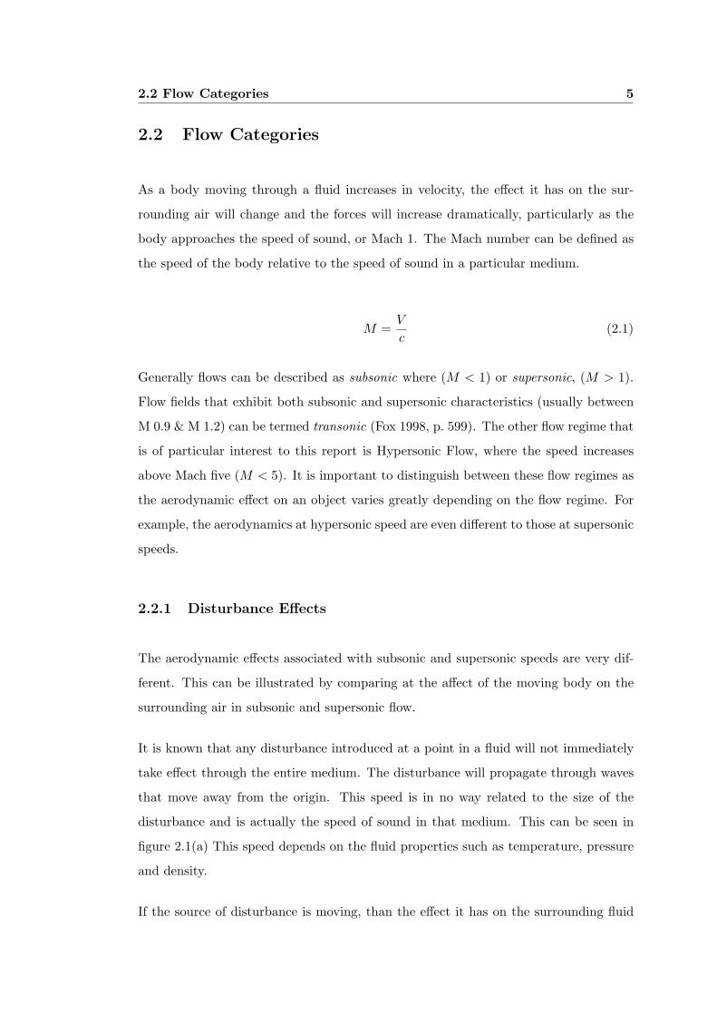
It is known that any disturbance introduced at a point in a fluid will not immediately
take effect through the entire medium. The disturbance will propagate through waves
that move away from the origin. This speed is in no way related to the size of the
disturbance and is actually the speed of sound in that medium. This can be seen in
figure 2.1(a) This speed depends on the fluid properties such as temperature, pressure
and density.
If the source of disturbance is moving, than the effect it has on the surrounding fluid
2.2 Flow Categories 6
will vary depending on its velocity. If the source is moving at a velocity less than
the speed of sound (M < 1), waves will still propagate away from the source in all
directions at the speed of sound (as illustrated by figure 2.1(b)). As the speed of the
source increases towards M1 these waves will become concentrated to a narrow region
in front of the disturbance source (shown by figure 2.1(c)).
Figure 2.1: Disturbance Effects(Duncan 1974, p. 159)
However, when the speed becomes greater than Mach 1, all of the spherical waves

2.2 Flow Categories 7
produced by the disturbance are swept downstream of the source. If the flow is steady,
the disturbance waves will lie within a circular cone (known as a Mach Cone) where
the source is at the apex (figure 2.1(d)). Outside of this cone, the fluid will remain
unaffected. The edges of the mach cone where the disturbance effect is concentrated
are known as Mach Waves.
When the velocity of the disturbance is supersonic, it presents a front of very rapid,
almost discontinuous compression to the oncoming fluid which is know as a Shock Wave
(Duncan 1974). In crossing a ’shock’ there is a rapid increase in pressure, a rapid rise
in the density and temperature of the fluid and a fall in velocity. This one of the
important phenomena associated with Supersonic and hypersonic flow. In fact, the
process of change over a shock wave is so rapid and the thickness of the wave is so
small that it is often treated as a discontinuity in the flow.
2.2.2 Hypersonic Flow
Hypersonic flow is defined as ”the regime where certain flow phenomena become pro-
gressively more important as the Mach Number is increased to higher values” (John
D. Anderson 1989, p. 13). Duncan (1974) describes Hypersonic flow as flow past a body
at sufficiently high Mach numbers that is characterised by the fact that the leading edge
shock waves lie close to the body surface. In some cases this can be as low as Mach
3, but as a rule of thumb is generally above Mach 5. Hypersonic flow is differentiated
by the way that the flow pattern undergoes little change with an increase in Mach
Number.
For a given flow deflection (or flow over a body), the density increase across the shock
wave becomes progressively larger as the flow speed increases. At these higher densities,
the mass flow behind the shock can more easily squeeze through a smaller area resulting
in a small distance between the shock wave and the body. This flowfield between the
shock wave and the hypersonic body is know as the shock layer. Some important
characteristics associated with hypersonic flow are:
• The shock waves are close to the body, (therefore thin shock wave theory can be
2.2 Flow Categories 8
used).
• Hypersonic flow creates high temperatures.
• There will be viscous interaction between the fluid and body.
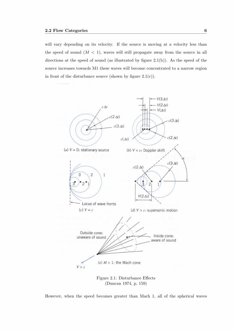
In Hypersonic Theory, for flow over simple shapes, it can be assumed that the speed and
direction of the gas particles in the freestream will remain unchanged until such time as
they strike the solid that is exposed to the flow. This flow model is termed Newtonian
Flow. In this flow model the normal component of the momentum of the approach-
ing particle is cancelled out, whereas the tangential component of the momentum is
conserved. This is illustrated by figure 2.2 where only the tangential component of
the velocity (U∞, t) is conserved, not the normal component (U∞, n) . Because energy
cannot be destroyed, the kinetic energy that is lost by the particles through contact
with the body is in turn released causing high temperatures at the contact surface.
Figure 2.2: Particle motion in Newtonian Flow(Bertin 1994, p. 6)
By using the momentum equation and the Newtonian flow model, the local pressure
on the body can be determined in terms of the pressure coefficient.
Pressure coefficient (Cp) (Bertin 1994, p. 6)
Cp =pw − p∞12ρ∞U2∞
= 2 sin2 θb = 2 cos2 φ (2.2)

2.3 Predicting Forces caused by Hypersonic Flow 9
Where number 2 represents the stagnation point pressure coefficient, Cpt2, for New-
tonian Flow (Bertin, p.6). (The stagnation point pressure coefficient relates to the
pressure at the point on the body where the fluid has zero velocity). This pressure
coefficient could then be used to calculate the normal and axial force coefficients. In
these equations the local body slope (relative to the flow) is represented by θb
Alternatively the equation can be written (Bertin 1994, p .279)
Cp = Cpt2 sin2 θb = Cpt2 cos2 φ (2.3)
This is termed Modified Newtonian Flow. For the modelling of flow over blunt bodies
the modified newtonian equation ( 2.3) is considerably more accurate than the standard
equation( 2.2) .
The ability to test in hypersonic flow in the USQ Gun Tunnel is very important as the
behaviour of the fluid in hypersonic flow is physically different from that in in subsonic
and even supersonic flow. (This can be further illustrated by comparing hypersonic
vehicles to subsonic aircraft.)
While the focus of this project is to actually measure aerodynamic forces in a controlled
environment, it is also important that the forces on a particular body in hypersonic
flow can be predicted whether this be analytically, or through computational methods.
2.3 Predicting Forces caused by Hypersonic Flow
There are various methods of predicting the forces that will act on a model during
hypersonic flow. One analytical method that will be suitable for this application as
mentioned previously is the modified Newtonian flow model.
In order to calculate the forces acting on the re-entry capsule the pressure distribution
must be calculated using the stagnation point pressure coefficient Cpt2 (Bertin p.287),
2.3 Predicting Forces caused by Hypersonic Flow 10
Cpt2 =[pt2
p1− 1
]2
γM21
(2.4)
Where the ratio of pressures pt2
p1can be found using (Bertin 1994, p. 288). This is the
ratio of the pressure difference across the shock wave.
pt2
p1=
[(γ + 1)M2
1
2
] γγ+1 [
γ + 12γM2
1 − (γ − 1)
] 1γ−1
(2.5)
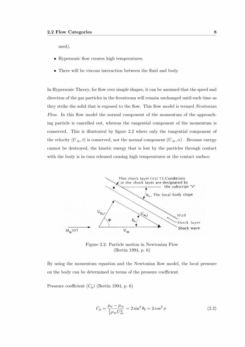
This pressure coefficient can also be checked using the graph in figure 2.3.
Figure 2.3: Variation of stagnation pressure coefficient with M(John D. Anderson 1989, p. 55)
The stagnation point pressure coefficient can then be used to determine the force co-
efficients (Bertin 1994, p. 468-470). The force coefficient equations (2.6 & 2.7) are
dependent on the body shape and angle of attack. The nomenclature for these equa-
tions for blunt bodies (similar to MUSES-C) can be seen in figure 2.4.
Normal Force Coefficient:

2.3 Predicting Forces caused by Hypersonic Flow 11
CN = 2Cp,t2
(RN
RB
)2
0.25 sinα cosα cos4 θc + sin α cosα sin θc cos θc×((RB/RN )−cos θc
tan θccos θc + ((RB/RN )−cos θc)2
2 tan θc
)
(2.6)
Axial Force Coefficient:
CA = 2Cpt2
(RN
RB
)2
(0.25 cos2 α(1− sin4 θc) + 0.125 sin2 α cos4 θc)+
tan θc(cos2 α sin2 θc + 0.50 sin2 α cos2 θc)×((RB/Rn)−cos θc
tan θccos θc + ((RB/RN )−cos θc)2
2 tan θc
)
(2.7)
Figure 2.4: Nomenclature for spherically blunted cones(Bertin 1994, p. 465)
Finally, by using the equations below the actual forces on the model can be predicted.
In this case, r is represented by RB.
FN = CNρ1U21 Πr2 (2.8)
FA = CAρ1U21 Πr2 (2.9)

2.4 Chapter Summary 12
2.4 Chapter Summary
This chapter has given a brief overview of the phenomenon associated with the various
flow regimes, in particular hypersonic flow.
It has also given an introduction to aerodynamic Forces and outlined how to estimate
the aerodynamic forces acting on the a blunt body (such as the Muses-C spacecraft).
Chapter 3
Hypersonic Aerodynamic Force
Measurement
3.1 Chapter Overview
In the design of aircraft it is important that the theoretical and computational predic-
tions (that have already been discussed) can be combined with an experimental testing
program.
Only real flight tests on a full scale model can create a completely accurate picture of
vehicle behaviour. However it is obvious that these tests can only occur after extensive
design, development, construction and therefore considerable cost. For this reason, the
majority of of experimental information is obtained from ground based testing facilities.
Since complete simulations of a flowfield cannot be recorded at ground based facilities,
it is important that the objectives of the tests are clearly outlined. Some common aims
of testing include; (Bertin 1994)
1. Obtaining data to define the aerodynamic forces and moments or heat trans-
fer distributions for configurations whose complex flowfields resist computational
modeling .
3.2 Types of Testing Facilities 14
2. Obtaining detailed data to be used in developing computational flow models (code
validation).
3. Determine measurements of parameters, such as heat transfer and drag that can
be compared to computed solutions.
Just as there are a numerous reasons for conducting hypersonic tests, there are a
number of different types of testing facilities. This chapter will describe some of the
major types of testing facilities and look at the different ways that aerodynamic forces
are measured. It will also include a brief description of the USQ Gun Tunnel and the
system that was employed to measure aerodynamic forces in hypersonic flows.
3.2 Types of Testing Facilities
There are a number of different types of testing facilities that can be used to replicate
the aerothermodynamic environment of re-entry capsules. The type of facility, due
to the differences in the flows created, can have a large bearing on how aerodynamic
forces will be measured at that facility. Four main types of ground based hypersonic
testing facilities are; Shock Tubes, Arc Heated test Facilities, Hypersonic win tunnels
and Ballistic free-flight ranges. These are outlined below.
3.2.1 Shock Tubes
A Shock Tube facility is one where a shock wave passes through a test gas, creating a
high-pressure/ high temperature environment (Bertin 1994).
This type of facility can be divided into two sections that are initially divided by a
diaphragm. One of the sections, know as the ”driver” section is filled with a gas at a
high pressure. The other section is filled with the ”driven” gas at a low pressure. As
the diaphragm bursts under the high pressure, the motion of the driver gas causes a
shock wave to move through the driven section creating the test flow.
One of the important features of this type of system is that the test time that is created

3.2 Types of Testing Facilities 15
can be as small as fractions of a millisecond. They are not very useful for the testing
of scale models.
3.2.2 Arc-heated Test Facilities
In an arc-heated test facility, the test gas is passed through a high-power electric arc
(inside a pressure vessel) and then through a converging/diverging nozzle. This creates
supersonic flow, and while the impact pressure and enthalpy that are created are similar
to re-entry conditions, the Mach number is generally low.
Arc-heated facilities are important because they can be used to
• Prevent condensation of the test gas during expansion to hypersonic Mach num-
bers
• To replicate the physical and chemical transformation of air for the study of
aerothermodynamics.
• To investigate the internal physical and Chemical changes of materials caused by
interaction with the high temperature environment.
Arc-heated test facilities can provide relatively high stagnation pressures for test times
greater than a minute.
3.2.3 Ballistic Free Flight Ranges
Range facilities allow for the free flight testing of a subscale model in a controlled
environment. This is done by shooting the model at hypersonic velocities through a
long range tank. The test gas can also be easily changed to simulate the entry of
different atmospheres.
The problem with free flight ranges is that often it is difficult to obtain experimental
measurements. In addition to this, the large accelerations that are experienced in

3.3 The USQ Gun Tunnel 16
testing mean that the model must be relatively small and simple to cope with the large
stresses that would be imposed.
3.2.4 Hypersonic Wind Tunnels
In hypersonic wind tunnels, a test gas is accelerated from a reservoir (at rest) through
a converging/ diverging nozzle creating hypersonic speeds in the test section. The
acceleration may be assumed to be isentropic.
Hypersonic wind tunnels are often categorised by their run time. Impulse facilities have
a run time of 1s or less. Intermittent tunnels have run times that range from a few
second to several minutes and Continuous tunnels can run for hours.
Obviously, as the run time of the wind tunnel decreases it becomes harder to take accu-
rate measurements of aerodynamic forces because the model will not meet equilibrium.
The accuracy of wind tunnel testing also relies heavily on the quality of the flow.
Hypersonic Wind tunnels are the area of most interest to this report as they have
similar characteristics to the USQ Gun Tunnel which has a run time of 25ms.
3.3 The USQ Gun Tunnel
The function of the USQ gun tunnel is to produce hypersonic airflow under controlled
conditions. The USQ gun tunnel is capable of producing an 80mm diameter flow, at
speeds of up to Mach 7 during a 25ms test time.
3.3.1 Facility Layout
The USQ Gun tunnel is located at the University of Southern Queensland (Toowoomba)
campus in the ’S Block’ basement.
For descriptive purposes, the Gun Tunnel can be divided into three main sections (this
3.3 The USQ Gun Tunnel 17
can be seen in figure 3.2).
1. Reservoir Section (Driver section at high pressure)
2. The tunnel and converging/ diverging nozzle (driven section)
3. The test section and dump tank (initially at low pressure)
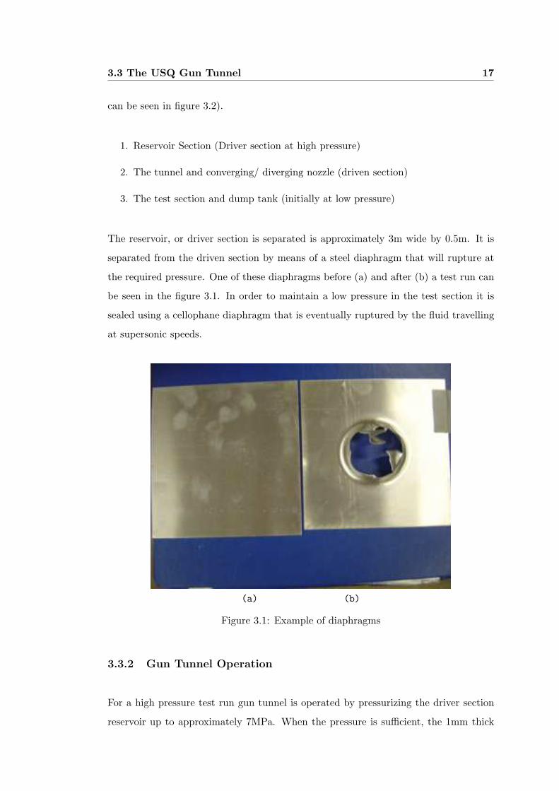
The reservoir, or driver section is separated is approximately 3m wide by 0.5m. It is
separated from the driven section by means of a steel diaphragm that will rupture at
the required pressure. One of these diaphragms before (a) and after (b) a test run can
be seen in the figure 3.1. In order to maintain a low pressure in the test section it is
sealed using a cellophane diaphragm that is eventually ruptured by the fluid travelling
at supersonic speeds.
(a) (b)
Figure 3.1: Example of diaphragms
3.3.2 Gun Tunnel Operation
For a high pressure test run gun tunnel is operated by pressurizing the driver section
reservoir up to approximately 7MPa. When the pressure is sufficient, the 1mm thick

3.3 The USQ Gun Tunnel 18
steel diaphragm will rupture allowing the lightweight plastic piston to travel at super-
sonic speeds (with a shock wave travelling in front of it) down the tunnel, compressing
the air in front of it. The tunnel section is approximately 5 meters long and 100 mm
in diameter. The fluid is then forced through a converging diverging nozzle, which
restricts the flow diameter to 80mm. At the exit of this nozzle is where the fluid is
accelerated to velocities of Mach 7 for a run time of up to 25 milliseconds. At the end
of the process the air finishes in the dump tank, which is depressurised at the end of
the run.
Figure 3.2: Diagram of Gun Tunnel layout
During each test, the stagnation pressure of the flow is measured using a pressure
transducer located at the nozzle. Not only is this important for the theoretical force
calculations, it also gives and indication of the quality of the flow.
The performance of the Gun Tunnel under high pressure operating conditions can be
seen in table 3.1. In this table, free flow conditions describe the actual flow conditions
that the model is exposed to. The free flow temperature is very low due to the isentropic
expansion that takes place in the nozzle to create hypersonic flow.

3.4 Force Measurement Systems 19
Performance Parameter ValueMach Number(M) 7Stagnation Pressure(Po) 6 MPaStagnation Temperature(T0) 750 KFree Flow Pressure 1.45 KPaFree Flow temperature 68.4 KInitial Density 28.9 kg/m3
Free Flow Density 0.0753 kg/m3
Free Flow Velocity 1150 m/sPressure Behind the Shock Wave 92.1 kPaStagnation Point Pressure Coefficient (Cpt2) 1.82
Table 3.1: Performance parameters of the Gun Tunnel
3.4 Force Measurement Systems
There are a number of different ways that forces on re-entry capsules can be measured
in ground based test facilities. The method of measurement often depends on the
performance of the facility itself, but can also depend on the type and accuracy of the
data required.
One thing that all impulse facilities have in common is that because of the sudden
impact of the aerodynamic forces on the model, the entire system will begin to oscillate
at its natural frequency. In a wind tunnel with a reasonable run time, the useful test
time would begin after these oscillations had been damped out. However in facilities
like the USQ Gun Tunnel with very short test times it is almost impossible to damp
out the oscillations and find the steady state. Also, the inertia forces of the oscillating
model and balance can add to the aerodynamic forces and moments.
In the past, measurement of aerodynamic forces in short duration test facilities has
been restricted because of the time that it takes for the model to reach equilibrium
with its support mechanisms. Force balances often rely on damping mechanisms or
filters to reduce the effects of the vibrations that are caused by the sudden impact of
the aerodynamic force (Mee 2003). Unfortunately at times the test time of the flow may
be too short to damp out these vibrations and in some cases the period of oscillation
of the model can be longer than the actual test time.

3.4 Force Measurement Systems 20
A number of techniques can be used to fix this problem. The natural frequency of
the system can be increased by making the force balance very stiff and the model very
light. Another option is to use accelerometers that can be placed on the model to detect
vibrations and compensate for the strain signals from the force balance. Alternatively
the model could be connected with flexible supports and its acceleration measured.
This can then be taken one step further and the model be allowed to ’fly free’ during
the test. This removes the effect of the support mechanism that decreases the natural
frequency of the system. In the case of the free flying model, the natural frequency
would be set only by the model size and the speed of the stress waves in the structure
of the model (Mee 2003).
A method was developed to measure the acceleration of a free flying model in a shock
tunnel (Storkmann 1998). The model was controlled by a mounting support that
releases the model just before the onset of the flow. During the test there are no
connecting parts between the model and the support system. The support system
does not cause the model to accelerate. The forces are then determined from the
accelerations and inertia matrix of the model using Newton’s Law. In this test it is
essential to have the model equipped with at least six accelerometers. Hence this would
be a very expensive system to set up.
The method that Mee used for force measurement in impulse test facilities involved the
connection of the model to a long hollow sting (Storkmann 1998). The setup hangs
in the wind tunnel from two shielded wires that can freely move in the flow direction.
In this case the stress waves that are introduced into the system are measured, rather
than the acceleration. The setup can be seen in figure 3.3.
Figure 3.3: Single-component stress-wave force-balance(Mee 2003)

3.4 Force Measurement Systems 21
An alternative method has been used in the SR3 wind tunnel. The SR3 wind tunnel
generates hypersonic nitrogen flows for a continuous run time. Hence it will not expe-
rience may of the difficulties associated with impulse facilities, however it is still worth
investigating. The force balance that is used in this case is connected by two wires
and utilizes three dynamometers to take measurements. This system allows for the
measurement of drag, lift pitching moment and centre of pressure with good accuracy.
Unfortunately this does not address the problem of the oscillation of the model because
the measurements at the SR3 wind tunnel can be taken over a few seconds.
A force balance that is similar in nature to the one at USQ was designed by Jessen
and Gronig (this is described in (Storkmann 1998)). They use a strain gauge balance
that is designed to work without any acceleration compensation. The balance is part
of the sting (or mounting arrangement) and is essentially independent of the model. In
this case, no acceleration gauges would be needed inside the model. This system can
be calibrated statically with high accuracy and achieves a high natural frequency in
excess of 1kHz.
After examining this system and its test results it is concluded in (Storkmann 1998),
that it is possible to determine aerodynamic loads without without compensation for
the inertia forces caused by the oscillation of the model and support system. That
is, provided the measurement time is longer than the lowest natural frequency of the
system-model balance. If the system is optimised in terms of weight and moment of
inertia to give a higher natural frequency, it will give more reliable measurements.
3.4.1 Calibration
In his paper, Mee discusses the calibration of force balances for hypersonic test facilities.
This calibration can be performed either by a hung weight test (that will be descried
in chapter 5), a self weight test, or a hammer pulse test. All these techniques have the
same underlying principle; by applying a know load, the response of the system can be
modeled.
An important point that is Mee makes is that calibrations should be performed when
3.5 The USQ Force Measurement System 22
the model is mounted in the test tunnel. This way, the characteristics of the tunnel
mounting arrangement can be included in the model response.
3.5 The USQ Force Measurement System
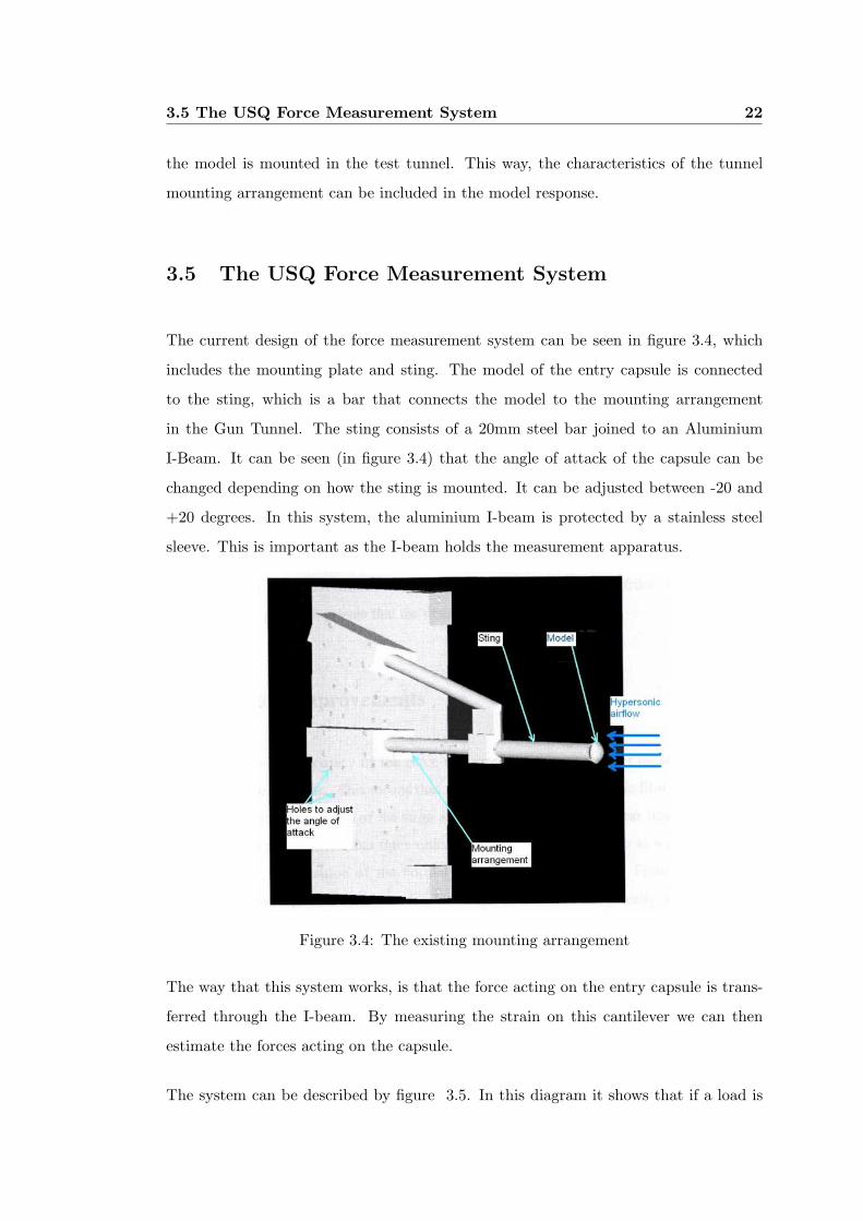
The current design of the force measurement system can be seen in figure 3.4, which
includes the mounting plate and sting. The model of the entry capsule is connected
to the sting, which is a bar that connects the model to the mounting arrangement
in the Gun Tunnel. The sting consists of a 20mm steel bar joined to an Aluminium
I-Beam. It can be seen (in figure 3.4) that the angle of attack of the capsule can be
changed depending on how the sting is mounted. It can be adjusted between -20 and
+20 degrees. In this system, the aluminium I-beam is protected by a stainless steel
sleeve. This is important as the I-beam holds the measurement apparatus.
Figure 3.4: The existing mounting arrangement
The way that this system works, is that the force acting on the entry capsule is trans-
ferred through the I-beam. By measuring the strain on this cantilever we can then
estimate the forces acting on the capsule.
The system can be described by figure 3.5. In this diagram it shows that if a load is
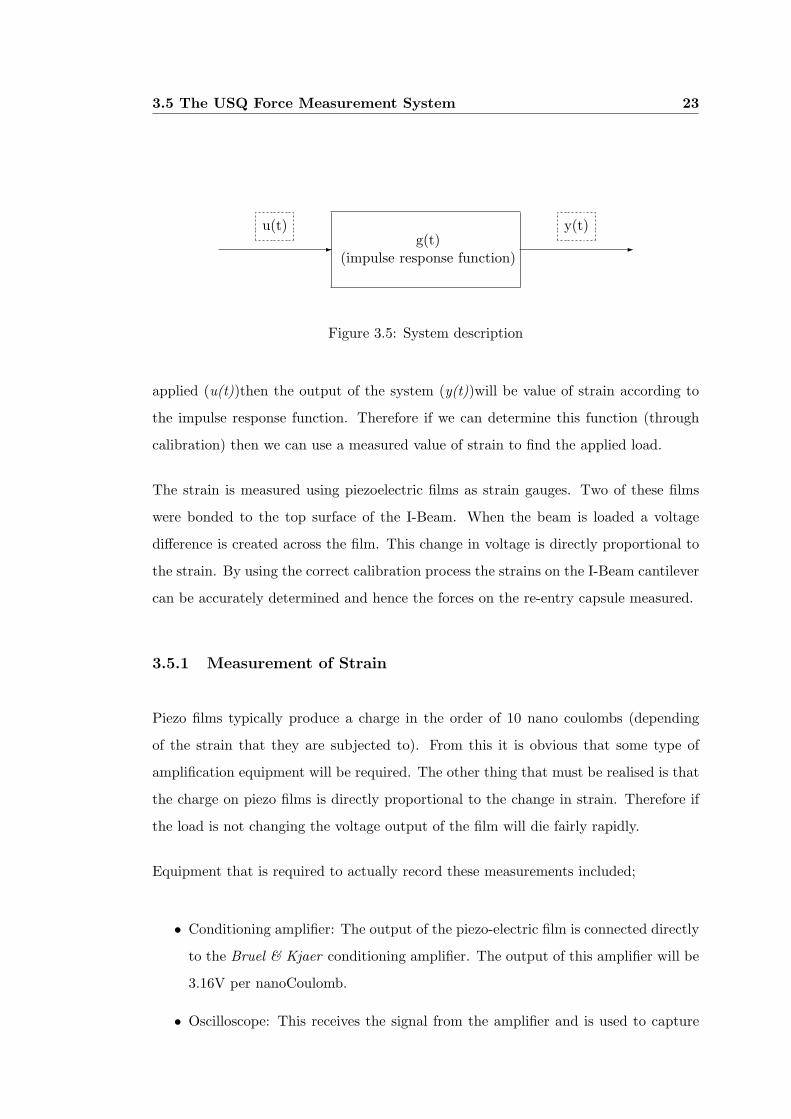
3.5 The USQ Force Measurement System 23
- g(t)(impulse response function)
-
u(t) y(t)
Figure 3.5: System description
applied (u(t))then the output of the system (y(t))will be value of strain according to
the impulse response function. Therefore if we can determine this function (through
calibration) then we can use a measured value of strain to find the applied load.
The strain is measured using piezoelectric films as strain gauges. Two of these films
were bonded to the top surface of the I-Beam. When the beam is loaded a voltage
difference is created across the film. This change in voltage is directly proportional to
the strain. By using the correct calibration process the strains on the I-Beam cantilever
can be accurately determined and hence the forces on the re-entry capsule measured.
3.5.1 Measurement of Strain
Piezo films typically produce a charge in the order of 10 nano coulombs (depending
of the strain that they are subjected to). From this it is obvious that some type of
amplification equipment will be required. The other thing that must be realised is that
the charge on piezo films is directly proportional to the change in strain. Therefore if
the load is not changing the voltage output of the film will die fairly rapidly.
Equipment that is required to actually record these measurements included;
• Conditioning amplifier: The output of the piezo-electric film is connected directly
to the Bruel & Kjaer conditioning amplifier. The output of this amplifier will be
3.16V per nanoCoulomb.
• Oscilloscope: This receives the signal from the amplifier and is used to capture

3.5 The USQ Force Measurement System 24
the data from the test run.
• Wavestar computer software: This takes the data from the oscilloscope and com-
piles it in tabular form. This allows for further analysis of the results

3.6 Chapter Summary 25
3.6 Chapter Summary
This chapter gave and overview of why ground based testing is important and looked
into various hypersonic test facilities. It also gave an overview of some existing hyper-
sonic force measurement systems.
In this section, an description was given of the USQ Gun Tunnel and how aerodynamic
forces are measured at hypersonic speeds in this facility.

Chapter 4
Analysis of Original System
4.1 Chapter Overview
In order to improve the existing force measurement system that is employed in the USQ
Gun Tunnel, it is important to know how the system works. Before any improvements
can be made, the system must be analysed to identify any problems and areas that
require modification.
This chapter will look at the results of the initial system and describe the ways that
these could be improved.
4.2 Original Results
The results that were obtained from previous measurements from a high pressure test
run (at Mach 7) in the Gun Tunnel, with an angle of attack of 10 degrees indicate
normal forces of 0.927N and Axial forces of 72.9N (Terhorst 2001).
As there are only two strain gauges, one located at the front of the I-Beam and one at
the back hence only two unknown variables can be found. Therefore, with the current
system, the position at which the forces will act on the model must be estimated when

4.2 Original Results 27
calculating the normal and axial forces. This location where the forces are assumed to
act is known as the centre of pressure.
As previously mentioned when the forces are determined for the entry capsule there
is not one steady force (or voltage) that is measured. Instead the whole system will
oscillate at the natural frequency of the arrangement. This means that an average
value of the force must be taken over a period of time. The time span where there is a
constant pressure exerted in which to take measurements will be 25ms at best.
The test run used by Terhorst(2001) to obtain his measurements provided good flow
conditions for 20ms. However the force measurement system provided useful measure-
ments for only 4 milliseconds, (from 23 milliseconds to 27 milliseconds) as can be seen
in figure 4.1). After this period the output is less useful and appears to be affected by
resonance or a second lower frequency. This may be improved by some type of damping
system. The frequency of the system in the hypersonic flow was determined to be 500
Hz (Terhorst 2001, pg. 81).
Figure 4.1: Results of the previous Force Measurement System
4.3 Bench testing of original system 28
4.2.1 Expected Results
The theoretical values obtained for these forces were 8.2185 N in the normal direction
and 78.3808N in the Axial direction. This can be compared to the measure values of
0.927N in the normal direction and 72.9N in the axial. From this data it can be seen
that the force prediction is reasonably accurate in the axial direction, however the error
associated with measuring normal forces is significant.
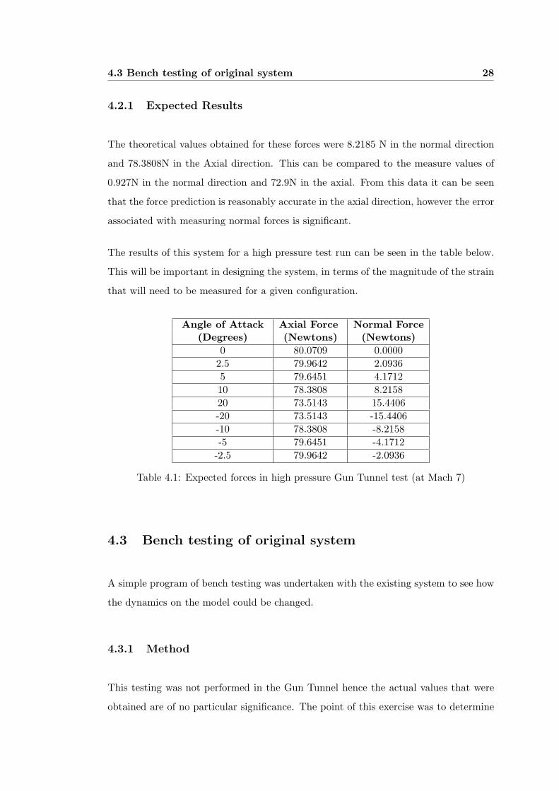
The results of this system for a high pressure test run can be seen in the table below.
This will be important in designing the system, in terms of the magnitude of the strain
that will need to be measured for a given configuration.
Angle of Attack Axial Force Normal Force(Degrees) (Newtons) (Newtons)
0 80.0709 0.00002.5 79.9642 2.09365 79.6451 4.171210 78.3808 8.215820 73.5143 15.4406-20 73.5143 -15.4406-10 78.3808 -8.2158-5 79.6451 -4.1712
-2.5 79.9642 -2.0936
Table 4.1: Expected forces in high pressure Gun Tunnel test (at Mach 7)
4.3 Bench testing of original system
A simple program of bench testing was undertaken with the existing system to see how
the dynamics on the model could be changed.
4.3.1 Method
This testing was not performed in the Gun Tunnel hence the actual values that were
obtained are of no particular significance. The point of this exercise was to determine

4.3 Bench testing of original system 29
how the natural frequency and damping properties of the sting/model system changed
as certain modifications were made.
For these tests the sting was clamped to a bench using two G-clamps. The model was
excited by being gently struck with a rigid object. The response of the system was
observed through the oscilloscope.
The original configuration was compared to a system where the I-beam was damped by
oil. Different methods of joining the back of the model to the protective sheath were
tested. These included Blu-Tac, tape and cardboard. All of these modifications were
an attempt to improve the original system which had no damping mechanism.
For each test the natural frequency was determined and the damping ratio calculated.
The most convenient way to determine the amount of damping present in the system
is to measure the rate of decay of free oscillations. Obviously, the more damping there
is, the larger the rate of decay. The natural logarithm of the ratio of two successive
amplitudes is know as the logarithmic decrement, δ. This can be determined using
equation 4.1, where X1Xn
is the ratio of the amplitude of oscillations over n cycles.
By using the experimental values,(an example of which can be seen in figure 4.2) and
equations 4.1 and 4.2 (W.T.Thomson 1988, p .33) we can determine the damping
factor, ζ. The ideal system would be critically damped, ζ = 1. However, from the
existing results of the measurement system, it is obvious that the existing system is
underdamped, meaning ζ < 1.
δ =1n
ln(X1
Xn) (4.1)
ζ =1√
1 + (2π/δ)2(4.2)

4.3 Bench testing of original system 30
Figure 4.2: Rate of decay of oscillation measured by the logarithmic decrement(W.T.Thomson 1988, p. 33)
4.3.2 Summary of Results
A summary of the results of bench testing of the existing system can be seen in table 4.2.
From this data it can be seen that there is a clear trend.
• As the damping of the system is increased the damped natural frequency is re-
duced.
This is shown by equation 4.3 where an increase in ζ would cause the damped natural
frequency to decrease.
ωd = ωn
√1− ζ2 (4.3)
While the natural frequency is reduced significantly, the value of the damping factor
remains quite low. Even with the addition of the oil damping, the system is still far
from being critically damped.
It must be noted that when the protective sheath was filled with oil, a second lower
natural frequency (≈ 250Hz) became obvious. This is important because it is the

4.4 Use of Piezoelectric Strain Gauges 31
lowest natural frequency of the system that is important when trying to increase the
accuracy of measurements (Chapter 3.4). The oil appeared to damp out the higher
frequency vibrations.
Fluid surrounding Sealing Method Natural Frequency Damping FactorI-Beam (Hz)
Air - 500 0.02Air Blu-Tac 416 0.03Oil - 263* 0.09Oil Blu-Tac 250 ??Oil Tape 240 0.14
Table 4.2: Summary of Initial Bench Testing
During this testing it became obvious that the piezo-electric films were susceptible to
interference. At times the output was effected by mains power (in the form of a 50 Hz
frequency) and even the movement of bodies around the model. This is one area that
would need to be addressed as it could have significant effect on the results.
4.4 Use of Piezoelectric Strain Gauges
The accuracy of the films has a large bearing on the accuracy of the force measurement
system as a whole. Therefore it is important to understand the limitations and possible
sources of error when using this equipment.
The use of piezoelectric films as strain gauges for the USQ Gun Tunnel has a number
of advantages. They can be easily cut to any size and bonded using commercially
available adhesives. More importantly, they are small and very light and can therefore
be attached to the system without effecting its dynamic properties or the motion of
the device. Piezo films also have a high mechanical strength and impact resistance.
Combined with this they have high stability, resisting most chemicals, moisture and
ultra violet radiation.
Piezoelectric films also have a wide frequency range (0.001 Hz - 1GHz) and large dy-
namic range suitable for measuring strains from 0.1 µε to 800 µε.
4.4 Use of Piezoelectric Strain Gauges 32
4.4.1 Material Properties
Piezoelectric films are polymer films based on polyvinylidene fluoride (PVDF) that have
piezoelectric properties that enable them to be used as electromechanical transducers.
They are particularly useful as dynamic strain sensors
The actual strain gauge is formed from a piece of this piezo film (20 - 50microns thick)
that has been metalised, and uniaxially oriented.
The piezoelectric films that have been used at USQ have a piezoelectric strain constant
of 69 × 10−3C/m2. This can be used to estimate the charge that will be created by a
certain strain.
Charge, Q = Area of F ilm× Strain× constant (4.4)
It has been shown that piezoelectric films exhibit a linear response to strains of up to
800 µε.
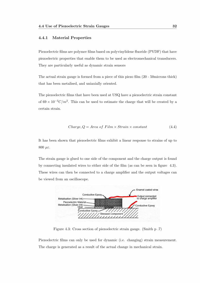
The strain gauge is glued to one side of the component and the charge output is found
by connecting insulated wires to either side of the film (as can be seen in figure 4.3).
These wires can then be connected to a charge amplifier and the output voltages can
be viewed from an oscilloscope.
Figure 4.3: Cross section of piezoelectric strain gauge. (Smith p .7)
Piezoelectric films can only be used for dynamic (i.e. changing) strain measurement.
The charge is generated as a result of the actual change in mechanical strain.

4.5 Required Areas of Improvement 33
4.4.2 Problems with Piezoelectric Strain Gauges
While the use of piezoelectric films as strain gauges offers a number of advantages,
there are also a few problems. These include,
• High sensitivity to changes in temperature: This must be considered, particularly
if the film is exposed to the flow stream.
• Can be sensitive to electromagnetic radiation/interference (EMI): This may be-
come a problem if the output level of the films becomes too small.
• AC Mains interference can be a problem with unshielded devices.
In order to improve the accuracy of results, these problems must be considered.
4.5 Required Areas of Improvement
From the analysis of the system it can be seen that there are a number of areas that
require improvement in order to increase the accuracy of the forces measured.
The first problem that has been identified is that the centre of pressure needs to be
identified through measurement, rather than estimation. This would reduce some of
the errors associated with the force calculation.
Secondly, the natural frequency of the model needs to be improved to increase the
number of oscillations in the measurement period. Ideally the natural frequency should
be above 1kHz. This value was achieved by Jessen and Gronig (see chapter 3.4) and
should be acceptable.
In addition to these improvements it would be desirable to improve the damping prop-
erties of the system. As it was seen in the initial bench testing, the system was under-
damped (table 4.2).
It was also noted that the piezoelectric films used for strain measurement were suscep-

4.5 Required Areas of Improvement 34
tible to background interference and were very sensitive to changes in temperature. In
order to get the most out of this system it is crucial that the effect of these external
influences are minimised.

4.6 Chapter Summary 35
4.6 Chapter Summary
This chapter has examined the current results of the USQ force measurement system
and compared them to expected outcomes. Some simple bench testing was undertaken
to characterise the dynamics of the original system. At the same time the original
system was modified to try and improve damping properties and natural frequency.
Using the gathered information conclusions were drawn about the required areas of
improvement.
These were:
1. The centre of pressure must be identified.
2. The natural frequency of the system must be increased.
3. The damping properties of the system should be improved.
4. The accuracy of the piezoelectric films should be improved through the reduction
of background interference.

Chapter 5
Improvement of the existing
System
5.1 Chapter Overview
This chapter will look at how to improve the USQ force measurement system in the
ways that were identified in chapter 4. These improvements will then be implemented
in the new design of the USQ Force measurement System which will be bench tested
to ensure the accurate measurement of strain in the cantilever.
5.2 Method of Improvement
5.2.1 Improving the Frequency Response
Some simple methods are to:
Decrease the mass of the model and/or cantilever. This might be done by using different
materials or reducing the amount of material used in the sting. Lighter metals or fiber
composites could be investigated. The effect of change in mass on the natural frequency
of the cantilever system can be seen in figure 5.1, where a 50 percent reduction in the
5.2 Method of Improvement 37
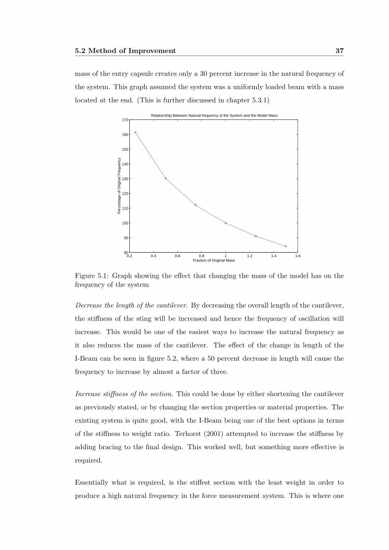
mass of the entry capsule creates only a 30 percent increase in the natural frequency of
the system. This graph assumed the system was a uniformly loaded beam with a mass
located at the end. (This is further discussed in chapter 5.3.1)
0.2 0.4 0.6 0.8 1 1.2 1.4 1.680
90
100
110
120
130
140
150
160
170
Fraction of Original Mass
Per
cent
age
of O
rigin
al F
requ
ency
Relationship Between Natural frequency of the System and the Model Mass
Figure 5.1: Graph showing the effect that changing the mass of the model has on thefrequency of the system
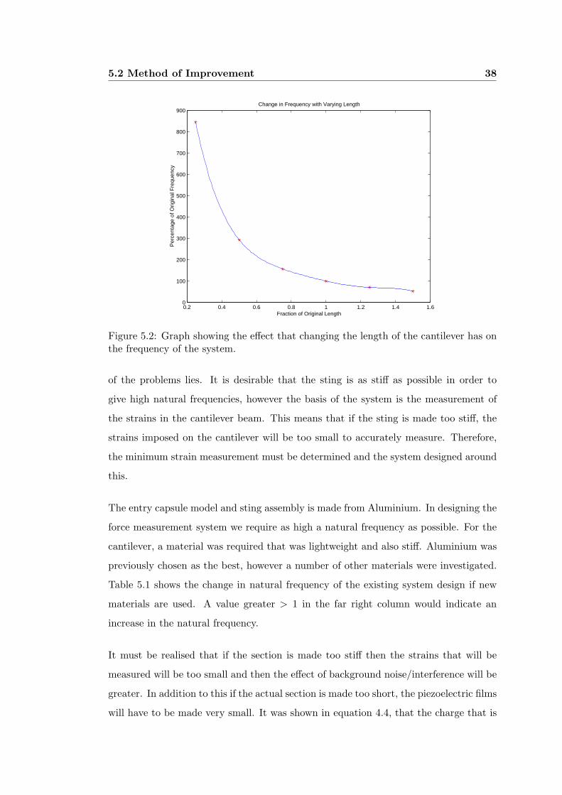
Decrease the length of the cantilever. By decreasing the overall length of the cantilever,
the stiffness of the sting will be increased and hence the frequency of oscillation will
increase. This would be one of the easiest ways to increase the natural frequency as
it also reduces the mass of the cantilever. The effect of the change in length of the
I-Beam can be seen in figure 5.2, where a 50 percent decrease in length will cause the
frequency to increase by almost a factor of three.
Increase stiffness of the section. This could be done by either shortening the cantilever
as previously stated, or by changing the section properties or material properties. The
existing system is quite good, with the I-Beam being one of the best options in terms
of the stiffness to weight ratio. Terhorst (2001) attempted to increase the stiffness by
adding bracing to the final design. This worked well, but something more effective is
required.
Essentially what is required, is the stiffest section with the least weight in order to
produce a high natural frequency in the force measurement system. This is where one
5.2 Method of Improvement 38
0.2 0.4 0.6 0.8 1 1.2 1.4 1.60
100
200
300
400
500
600
700
800
900Change in Frequency with Varying Length
Per
cent
age
of O
rigin
al F
requ
ency
Fraction of Original Length
Figure 5.2: Graph showing the effect that changing the length of the cantilever has onthe frequency of the system.
of the problems lies. It is desirable that the sting is as stiff as possible in order to
give high natural frequencies, however the basis of the system is the measurement of
the strains in the cantilever beam. This means that if the sting is made too stiff, the
strains imposed on the cantilever will be too small to accurately measure. Therefore,
the minimum strain measurement must be determined and the system designed around
this.
The entry capsule model and sting assembly is made from Aluminium. In designing the
force measurement system we require as high a natural frequency as possible. For the
cantilever, a material was required that was lightweight and also stiff. Aluminium was
previously chosen as the best, however a number of other materials were investigated.
Table 5.1 shows the change in natural frequency of the existing system design if new
materials are used. A value greater > 1 in the far right column would indicate an
increase in the natural frequency.
It must be realised that if the section is made too stiff then the strains that will be
measured will be too small and then the effect of background noise/interference will be
greater. In addition to this if the actual section is made too short, the piezoelectric films
will have to be made very small. It was shown in equation 4.4, that the charge that is

5.2 Method of Improvement 39
Material Density,ρ Modulus of Natural Frequency compared(kg/m3) Elasticity,E (Pa) Frequency,fn (Hz) to aluminium ( fn
fn(A))
Aluminium 2700 7.00× 10¹⁰ 744.81 1.0000Steel 7700 2.07× 10¹¹ 759.83 1.0186Titanium Alloy 4400 1.14× 10¹¹ 745.94 1.0015Brass 8300 1.10× 10¹¹ 533.51 0.7163Zinc Alloy 6600 8.30× 10¹⁰ 519.69 0.6978
Table 5.1: Effect of alternative materials on the natural frequency
produced by the piezoelectric strain gauge is directly proportional to its area. Hence
the use of smaller films would lead to a smaller charge output. This would increase the
effect of background noise.
From the information presented here, it can be seen that the most logical way to increase
the natural frequency of the system is to reduce the length of the aluminium I-Beam.
By changing materials there is no real advantage gained. The reduction of the mass
of the model would cause some increase in natural frequency, however the reduction
in the length of the cantilever appears to be the best option. If its length is halved,
the natural frequency should be approximately increased by a factor of three almost
(figure 5.2).
5.2.2 Improving the Damping Properties
The improvement of the damping properties of the sting will help to give clearer results
which will in turn make analysis easier.
Simple experiments were performed on the existing model to calculate the damping
factor, which was in the order of 10−3. A critically damped system has a damping
factor of one, which indicates the current system in extremely under-damped and there
is significant room for improvement. The damping properties could be improved by
connecting the back of the entry capsule model to the protective sleeve with a flexible
connection.
Another method is to fill the protective sleeve with oil, which would be sealed at the
5.2 Method of Improvement 40
back of the entry capsule. This would mean the entire I-Beam was submerged in oil.
It was shown that this did increase damping, but not significantly. This would have to
be set up very carefully to ensure the surrounding fluid does not affect the strain gauge
measurements. The use of oil might also offer some advantages in terms of reducing
the heating effects on the strain gauges.
Bench testing revealed that while the use of oil as a damping mechanism did increase
the damping factor in comparison to the undamped system, it didn’t offer any real
advantage to the system. This was because the damping factor still remained quite
low. If anything, the addition of the oil would cause problems in trying to keep the
system sealed. Leaking would be a problem where the wires exit the protective sheath.
There will be some type of flexible connection between the model and protective sleeve
(probably electrical tape). This may improve damping properties slightly, but its pri-
mary use is be to prevent any of the flow getting to the piezo films. Hence this would
also eliminate any temperature effects. This is an improvement on the original system,
and will help to esure that the piezoelectric films are not influenced by temperature
changes during the test.
5.2.3 Improving the Piezoelectric Output
As was noted earlier the piezoelectric films were susceptible to interference. This prob-
lem was compounded by the fact that the power for S-Block runs through the basement
where the Gun Tunnel is located. With the existing system, the films were bonded to
the sting using a conductive epoxy. This meant that there was a very large metal area
that was connected to the piezoelectric films that also had the ability to increase the
amount of interference that was received.
Initially an attempt was made to improve the piezoelectric film application procedure.
The idea of this was to make the piezo film and its wires a discreet system, such that
it was glued to the I-Beam but in no way electrically connected. This would hopefully
reduce the amount of interference that could influence the measurements. The basic
procedure that was followed was:
5.2 Method of Improvement 41
1. Bond wires to both sides of the Piezoelectric film using a conductive (silver based)
epoxy.
2. Cover the conductive epoxy on the underside with tape to prevent electrical con-
tact with the stressed member.
3. Then bond the piezoelectric film to the stressed member using araldite.
The idea with this was that the araldite would prevent a connection between the film
and the I-Beam. However this was not the case and contact was still made. This could
probably be prevented by applying tape to the entire underside of the piezoelectric film,
but this would compromise the strength of the bond between the film and the stressed
member.
The other option was to shield the device. This was investigated during the bench
testing where aluminium foil was used to shield the wires and the sting/model system.
It did make a considerable difference, but when moved to S-Block the 50Hz frequency
of the mains power was still an issue. However once the model was actually mounted in
the test section of the Gun Tunnel, the problem was removed. Presumably the 10mm
thick steel that forms the test section acted as a shield.
This means that while the attempt to improve the application procedure of piezoelectric
strain gauges didn’t succeed, accurate measurements can still be taken provided the
model is either shielded with aluminium foil or preferably is mounted in the Gun Tunnel.
5.2.4 Accurately Determining the Centre of Pressure
When estimating the force acting on a surface due to a certain flow, the pressures and
shear stress over the surface can be integrated over that surface to give a resultant force
(R). This force can be assumed to act at the centre of pressure of the model. Figure
5. shows a typical location of the centre of pressure (cp) with the Normal(N) and
axial(A) components of the resultant force (R). The location of the centre of pressure
is described by xcp and ycp. This diagram shows a pointed cone body shape, however
the priciple is the same for blunted bodies like MUSES-C.

5.3 Design of the New System 42
Figure 5.3: Location of the centre of pressure(Bertin 1994, p. 442)
One major area of improvement is to modify the force measurement system so that
the centre of pressure location can be determined and the normal and axial forces are
predicted accurately.
The simplest way to do this is to use more strain gauges. The addition of an extra film
on the underside of the I-Beam would allow for the centre of pressure to be identified,
however a fourth strain gauge would be ideal. This would allow for the identification
of the exact location of the centre of pressure.
5.3 Design of the New System
Taking into account the required areas of improvement and the various ways to make
these improvements, a new system was designed. This adopted the features of the old
system, but with a few simple changes.
• The length of the Aluminium I-beam was reduced by 40mm. This is approxi-
mately half of the original length and should lead to a significant increase in the
natural frequency of the system. The new component is shown in frigure B.1.
• Four Piezoelectric films were applied to be used as strain gauges. These piezo
films are roughly the same size of as the original ones (10×20mm) and are located
on the top and bottom of the aluminium I-beam.

5.3 Design of the New System 43
• The protective sheath was changed to a suitable length and will be connected
to the model using electrical tape to reduce any flow effects on the piezoelectric
strain gauges.
The new system setup can be seen in figure 5.4. (The protective sleeve has not been
put on in this picture to allow the position of the strain gauges to be seen.)
Figure 5.4: New system setup (with piezoelectric strain gauges)
5.3.1 Frequency Prediction
With the new system specified it is important that its natural frequency is modeled to
ensure it will be suitable.
An appropriate way to do this is to tread the system as a uniformly loaded beam with
a mass located at the end (see figure 5.5).
The frequency for this system can be modelled by looking at the effect of the model
and the beam separately.
The cantilever I-beam will be looked at first. The frequency of the cantilever beam is
calculated using equation 5.1 (W.T.Thomson 1988, p. 302)
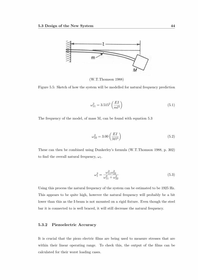
5.3 Design of the New System 44
(W.T.Thomson 1988)
Figure 5.5: Sketch of how the system will be modelled for natural frequency prediction
ω211 = 3.5152
(EI
ml3
)(5.1)
The frequency of the model, of mass M, can be found with equation 5.3
ω222 = 3.00
(EI
Ml3
)(5.2)
These can then be combined using Dunkerley’s formula (W.T.Thomson 1988, p. 302)
to find the overall natural frequency, ω1.
ω21 =
ω211ω
222
ω211 + ω2
22
(5.3)
Using this process the natural frequency of the system can be estimated to be 1925 Hz.
This appears to be quite high, however the natural frequency will probably be a bit
lower than this as the I-beam is not mounted on a rigid fixture. Even though the steel
bar it is connected to is well braced, it will still decrease the natural frequency.
5.3.2 Piezoelectric Accuracy
It is crucial that the piezo electric films are being used to measure stresses that are
within their linear operating range. To check this, the output of the films can be
calculated for their worst loading cases.
5.3 Design of the New System 45
It was previously stated that the piezoelectric output would measure stains as small as
0.1 microstrain. This lower limit is set by the noise from the piezoelectric element and
its hardware. This value of strain can be applied to the new system to determine the
accuracy to which forces can be measured.
For this calculation, the piezoelectric films closest to the model will be used as these
will record the smallest values of strain. This is due to the smaller bending moment at
the closer strain gauges which is associated with any normal force. It was found that a
normal force of 0.14N would produce the minimum value 0.1 microstrain.
The system will also be checked for the axial force that would be required to generate
0.1 microstrain. The force needed for the minimum strain measurement is 0.45N which
is larger than the force required in the normal direction. It can be seen from this, that
the force measurement system will at best measure forces to an accuracy of 0.45N. This
should be acceptable.
It was also noted previously that the piezoelectric films would behave linearly up to
800 microstrain. Therefore we must check that in the maximum loading conditions this
value of strain is not reached. The largest strains will be experienced at the largest
angle of attack due to increased bending stresses. It was estimated that at an angle of
attack of 20 degrees during a high pressure run, the forces present would be:
• Normal Force = 15.4 N
• Axial Force = 73.5 N
This can be considered as the worst load case, in which the maximum stresses will exist
at the piezoelectric films at the rear of the I-Beam (furthest away from the model). The
stresses that will be experienced here will be approximately 3.5MPa which will cause
a strain of 50µε. This is well below the maximum value of strain.
These calculations show that relationship between the applied force and the piezoelec-
tric output will remain linear during high pressure hypersonic tests in the USQ Gun
Tunnel. The system will also support larger models without reaching the maximum
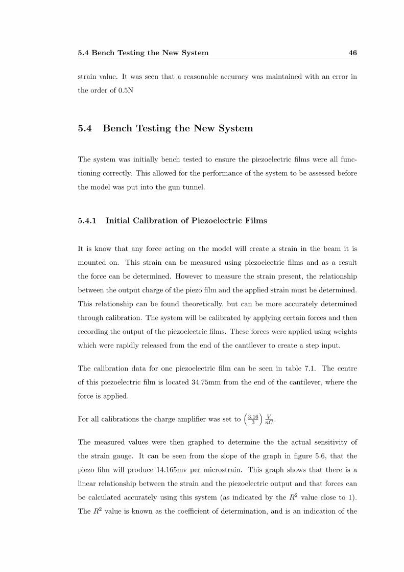
5.4 Bench Testing the New System 46
strain value. It was seen that a reasonable accuracy was maintained with an error in
the order of 0.5N
5.4 Bench Testing the New System
The system was initially bench tested to ensure the piezoelectric films were all func-
tioning correctly. This allowed for the performance of the system to be assessed before
the model was put into the gun tunnel.
5.4.1 Initial Calibration of Piezoelectric Films
It is know that any force acting on the model will create a strain in the beam it is
mounted on. This strain can be measured using piezoelectric films and as a result
the force can be determined. However to measure the strain present, the relationship
between the output charge of the piezo film and the applied strain must be determined.
This relationship can be found theoretically, but can be more accurately determined
through calibration. The system will be calibrated by applying certain forces and then
recording the output of the piezoelectric films. These forces were applied using weights
which were rapidly released from the end of the cantilever to create a step input.
The calibration data for one piezoelectric film can be seen in table 7.1. The centre
of this piezoelectric film is located 34.75mm from the end of the cantilever, where the
force is applied.
For all calibrations the charge amplifier was set to(
3.163
)VnC .
The measured values were then graphed to determine the the actual sensitivity of
the strain gauge. It can be seen from the slope of the graph in figure 5.6, that the
piezo film will produce 14.165mv per microstrain. This graph shows that there is a
linear relationship between the strain and the piezoelectric output and that forces can
be calculated accurately using this system (as indicated by the R2 value close to 1).
The R2 value is known as the coefficient of determination, and is an indication of the

5.4 Bench Testing the New System 47
Mass Force Stress Strain ×106 Measured Voltage(kg) (N) (MPa) (mV)
0.0000 0.000 0.000 0.000 00.6160 6.043 0.968 13.83 1981.1200 10.99 1.760 25.15 3601.6160 15.85 2.540 36.28 5242.1200 20.80 3.332 47.60 664
Table 5.2: Important values for calibration of a piezoelectric strain gauge
strength of the linear relationship between strain and the output voltage. A perfect
corellation would have an R2 value of 1.0.
Figure 5.6: Graph used for calibration of piezoelectric films
This process was repeated for all four piezoelectric films and all exhibited similar prop-
erties. Even though the sensitivity of some of the films was different, the degree of
accuracy was much the same with a very strong linear relationship between strain and
measured voltage.
5.4.2 Expected Piezoelectric Output
The expected sensitivity of the piezoelectric films can be calculated using equation 4.4.
For a value of 1µε with the piezo film area of 2× 10⁻⁴m2 the expected charge will be.

5.4 Bench Testing the New System 48
Charge = 1E−6 × 2× 10−4 × 69× 10−3
= 1.38e−11 Coulombs
= 0.0138 nC
Because the charge amplifier is set to(
3.163
)VnC , the voltage that will be produced by
this charge is;
V oltage =(
3.163
)× charge
= 0.0145V
= 14.5 mV
Therefore the piezoelectric films should produce 14.5 mVµε . This is very close to the
results that were found during the calibration of the first piezoelectric film. The sen-
sitivity of the other piezoelectric films were;11.0mVµε ,14.9mV
µε ,16.9mVµε . These also are
reasonably close to the expected values.
This initial bench testing has shown that the Piezoelectric films are working accurately
and are producing charges very close to the theoretical values.
5.4.3 Frequency Response
The natural frequency of the new system was also tested. This test was performed in
the USQ Gun Tunnel.
In the first case (see figure 5.7) the natural frequency was seen to be approximately
1.1kHz.
When the model was taped to the protective sheath the frequency remained virtually
unchanged. Figure 5.8 shows the frequency response of the model with tape connection

5.4 Bench Testing the New System 49
−0.01 −0.005 0 0.005 0.01 0.015 0.02−2500
−2000
−1500
−1000
−500
0
500Natural Frequency of the Model (with no tape)
Pie
zo O
utpu
t (m
V)
Time (s)
Figure 5.7: The frequency response of the system
−0.01 −0.005 0 0.005 0.01 0.015 0.02−400
−200
0
200
400
600
800
1000Natural Frequency of the model (with tape)
Pie
zo O
utpu
t (m
V)
Time (s)
Figure 5.8: The frequency response of the system with tape connection

5.5 Chapter Summary 50
5.5 Chapter Summary
This chapter has given an overview the new design of the force measurement system
and the factors that were taken into consideration when designing this system.
Calculations were also performed to ensure the piezoelctric films would be exposed to
strains within their linear operating range.
The perfomance of this system was tested to ensure it had improved as required. The
main improvement was that the natural frequency has increased to approximately
1.1kHz from the original value of 500Hz.
The changes to the USQ Force measurement system include:
• The I-beam was modified to increase the natural frequency
• Additional piezoelectric films were added to allow for the identification of the
centrof of pressure
• Tape was used to seal the isolate the piezoelectric films(within the protective
sleeve)from the flow.
The accuracy of the system was checked though calibration and was seen to be quite
good with a variation in the sensitivity of the piezoelectric film of less than 2%.

Chapter 6
Test Run Setup
6.1 Chapter Overview
For the first test run the model will be exposed to the flow at zero angle of attack.
Thus only axial forces will be experienced by the model. While this will not assess the
systems ability to measure normal forces, it will provide insight into the accuracy of the
piezoelectric films in the Gun Tunnel operation. Because of the nature of axial loading,
all strain gauges should experience the same strain and therefore should predict the
same value of force.
This test will be conducted at lower pressures of approximately 3MPa. This will create
smaller forces than a high pressure test run, but will importantly still be operating at
Mach 7.
This chapter will give an overview of how the force measurement system will be set up
for the first low pressure test run. The settings of electrical equipment will be described.
In addition to this, insight will be given into the problems that were experienced while
setting up for the test run.

6.2 Measurement Setup 52
6.2 Measurement Setup
When setting up the force measurement system in the Gun Tunnel the sting was first
positioned, then all wires were connected. When this was done, the response of all of
the piezoelectric films was checked. Finally the protective sheath was slid into position
and the model was screwed onto the end of the cantilever. Again the films were checked
again to ensure all were functioning properly.
To assist with the testing procedure, the amplifier and oscilloscope had to be positioned
to allow for easy operation. For testing in the USQ Gun Tunnel, the charge amplifier
was positioned on top of the dump tank (close to the test section) and was connected
to the oscilloscope using coaxial cable. The oscilloscope was positioned near the barrel
of the Gun Tunnel, where it could be connected to the computer by serial cable.
For any test run, it is important that all measurement devices are set to record maxi-
mum detail for greater accuracy without missing any of the signal.
6.2.1 Oscilloscope
The voltage was be set to 1 Volt per division. This may be a little too large, but
will ensure that all of the data is recorded. It must be realised that if the voltage
being measured goes outside the set range of the oscilloscope, the missing data cannot
be retrieved. Because the number of tests that can be performed is limited, we must
ensure that this does not happen.
The oscilloscope will be set to a time scale of 2.5ms per division. This will allow for
the measurement of the full 25ms run time.
It is also vital that the oscilloscope is triggered to start recording at exactly the right
time. The oscilloscope will be triggered externally by means of the pressure transducer.
The oscilloscope must also be set to trigger only once (single trigger) to ensure that
the data is not overwritten if it is re-triggered.

6.3 Connection of piezoelectric films 53
6.2.2 Charge amplifier
The charge amplifier was set to produce(
3.163
)V per nanocoulomb. It has the capacity
for four separate channels.
Input to the charge amplifier is through a microdot connection. The output of the
amplifier is through BNC plugs, all of which are located on the back of the unit.
The amplifier had the option of battery operation, but was connected through mains
power due to problems with the battery.
6.3 Connection of piezoelectric films
In order to connect the piezoelectric films to the to the conditioning amplifier, the
enamel coated wires that were connected to the strain gauge were soldered to BNC
plugs located inside the wall of the test section. A connection was then made from
these plugs to the amplifier (as can be seen in figure 6.1). This means that the test
section remains completely sealed during the test.
Figure 6.1: Location of BNC connection on test section wall
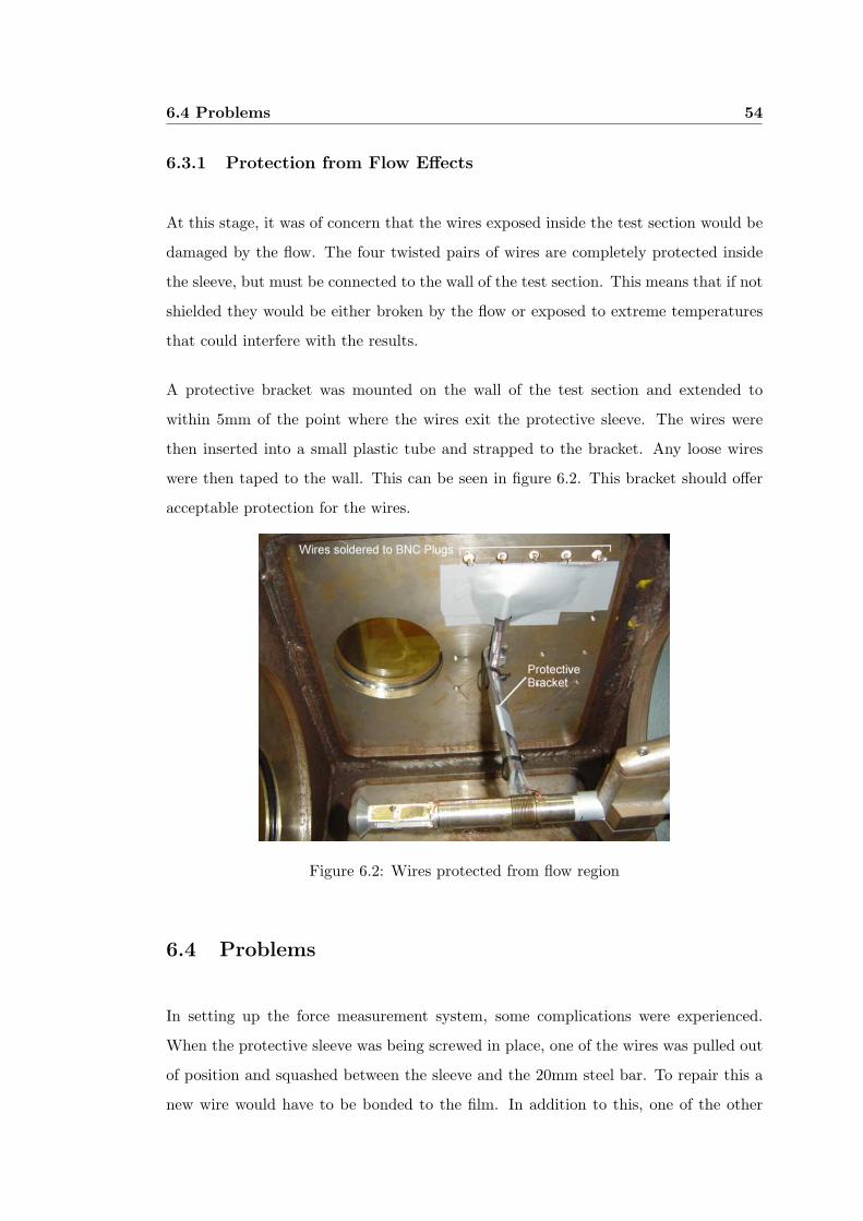
6.4 Problems 54
6.3.1 Protection from Flow Effects
At this stage, it was of concern that the wires exposed inside the test section would be
damaged by the flow. The four twisted pairs of wires are completely protected inside
the sleeve, but must be connected to the wall of the test section. This means that if not
shielded they would be either broken by the flow or exposed to extreme temperatures
that could interfere with the results.
A protective bracket was mounted on the wall of the test section and extended to
within 5mm of the point where the wires exit the protective sleeve. The wires were
then inserted into a small plastic tube and strapped to the bracket. Any loose wires
were then taped to the wall. This can be seen in figure 6.2. This bracket should offer
acceptable protection for the wires.
Figure 6.2: Wires protected from flow region
6.4 Problems
In setting up the force measurement system, some complications were experienced.
When the protective sleeve was being screwed in place, one of the wires was pulled out
of position and squashed between the sleeve and the 20mm steel bar. To repair this a
new wire would have to be bonded to the film. In addition to this, one of the other

6.4 Problems 55
piezoelectric films ceased to work for unknown reasons.
Under normal circumstances, this problem could be fixed in a couple of days, how-
ever due to time constraints, the test was performed with only two piezoelectric films
working. This is not critical for a test with zero angle of attack.

6.5 Chapter Summary 56
6.5 Chapter Summary
This chapter has given a detailed description of the setup for the force measurement
system in the USQ Gun Tunnel. This included not only the physical setup, but also
the settings of the electrical equipment. In addition to this, the aims of the testing
have been outlined.

Chapter 7
Results and Discussion
7.1 Chapter Overview
This chapter will present the results of the low pressure test run. Theses results will
be used to calculate the forces on the model. These forces will then be compared to a
theoretical prediction based on the measured pressure.
7.2 Flow Quality
The first thing to examine with the test run is the output of the pressure transducer.
This will give an indication of the time period where the forces can be measured.
Obviously the forces on the model will only simulate atmospheric re-entry when the
pressure is relatively steady.
The pressure that was measured can be seen in figure 7.1. In this graph the red line
represents the pressure. The region of steady flow was determined by visual inspection
and is between the two vertical black lines. between these lines (in black) is a least
squares fit to the pressure data. The average value of this function is the pressure value
that will be used for the average pressure calculations.
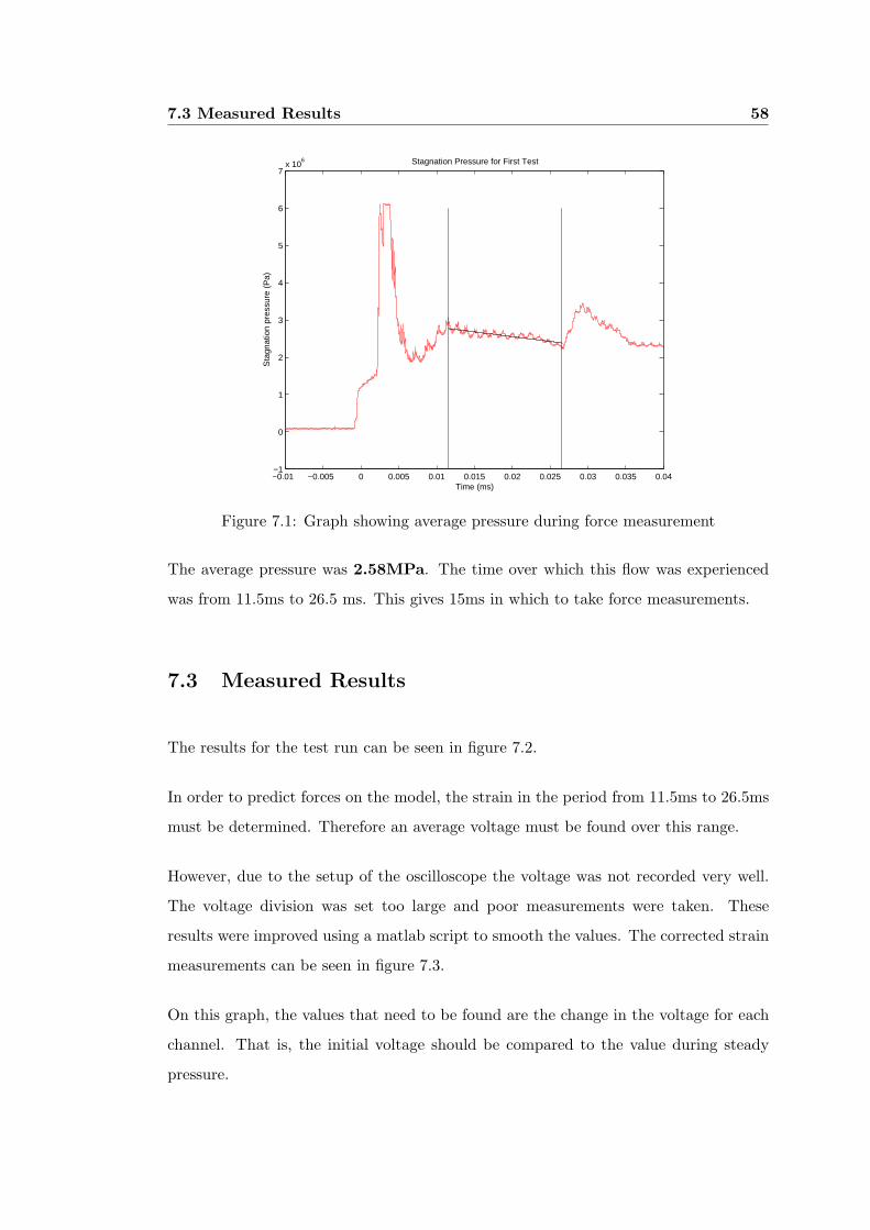
7.3 Measured Results 58
−0.01 −0.005 0 0.005 0.01 0.015 0.02 0.025 0.03 0.035 0.04−1
0
1
2
3
4
5
6
7x 10
6
Time (ms)
Sta
gnat
ion
pres
sure
(P
a)
Stagnation Pressure for First Test
Figure 7.1: Graph showing average pressure during force measurement
The average pressure was 2.58MPa. The time over which this flow was experienced
was from 11.5ms to 26.5 ms. This gives 15ms in which to take force measurements.
7.3 Measured Results
The results for the test run can be seen in figure 7.2.
In order to predict forces on the model, the strain in the period from 11.5ms to 26.5ms
must be determined. Therefore an average voltage must be found over this range.
However, due to the setup of the oscilloscope the voltage was not recorded very well.
The voltage division was set too large and poor measurements were taken. These
results were improved using a matlab script to smooth the values. The corrected strain
measurements can be seen in figure 7.3.
On this graph, the values that need to be found are the change in the voltage for each
channel. That is, the initial voltage should be compared to the value during steady
pressure.

7.3 Measured Results 59
−10 −5 0 5 10 15 20 25 30 35 40−200
−100
0
100
200
300
400
Time (ms)
Out
put (
mV
)
Voltage output from Low Pressure Test
piezo film #2peizo film #1
Figure 7.2: Results of strain measurement system for the test run
−10 −5 0 5 10 15 20 25 30 35 40−100
−50
0
50
100
150
Time (ms)
Out
put (
mV
)
Smoothed output from Low Pressure Test
piezo film #2peizo film #1
Figure 7.3: Smooth results of test run

7.3 Measured Results 60
The change in voltage for channel one is: 59.83mV
The change in voltage for channel two is: 38.87mV
From examination of the results, the natural frequency was determined to be approxi-
mately 500Hz. This is significantly lower than the 1.1kHz that was expected.
7.3.1 Piezoelectric Response
To check the response of the piezoelectric films and ensure that the measurement was
triggered at the right time, it would be helpful to plot the strain measurement on the
same axis as the pressure printout. Figure 7.4 shows that the films triggered at the
right time and even picked up small fluctuations in pressure towards the end of the run.
This graph is not drawn to scale and was only used to check the piezoelectric response.
Figure 7.4: Graph of response of piezoelectric films to pressure changes

7.4 Finding the Aerodynamic Force 61
7.4 Finding the Aerodynamic Force
7.4.1 Calibration
The system was calibrated after the test in the USQ Gun Tunnel, without changing
the setup. This means that the calibration will give and accurate indication of the
piezoelectric sensitivity during the test run. An example of the measurements recorded
during calibration can be seen in figure.
−10 −5 0 5 10 15 20
0
100
200
300
400
500
Callibration Plot for 1000g Mass
Pie
zo O
utpu
t (m
V)
Time (ms)
Figure 7.5: Example of calibration data
On this graph, the rapid change in voltage indicates the point where the masses were
released. The value that needs to be calculated is the total change in voltage when the
masses are cut. By doing this for a number of different masses, the sensitivity of the
piezoelectric films can be found quite accurately. A summary of the calibration results
can be seen in table 7.1 for the first piezoelectric film and table 7.2 for the second.
This data was then graphed to get the average value of sensitivity. This can in figures 7.6
and 7.7.

7.4 Finding the Aerodynamic Force 62
Figure 7.6: Graph used to determine sensitivity of first Piezo film
Figure 7.7: Graph used to determine sensitivity of second Piezo film

7.4 Finding the Aerodynamic Force 63
Hanging Mass Expected Strain Measured Voltage Sensitivity(kg) (µε) (mV) mV/µε
0.0000 0.000 0.000 na0.6179 13.874 182.0 13.121.1159 25.056 322.7 12.881.6179 36.327 459.7 12.652.1159 47.509 631.0 13.28
Table 7.1: Data from calibration of no. 1 Piezo film
Hanging Mass Expected Strain Measured Voltage Sensitivity(kg) (µε) (mV) mV/µε
0.0000 0.000 0.000 na0.6179 4.2918 38.794 9.041.1159 7.7510 75.052 9.681.6179 11.239 103.57 9.222.1159 14.6971 143.60 9.77
Table 7.2: Data from calibration of no. 2 Piezo film
From this calibration it has been that;
• The sensitivity of piezoelectric film 1 = 13.03 mVµε
• The sensitivity of piezoelectric film 2 = 9.56 mVµε
7.4.2 Force Calculation
Using the sensitivities from the calibration, the strain in the cantilever can be calcu-
lated. From this strain, the axial force during the test run can be determined. A
summary of the calculations can be seen in table 7.3.
Piezoelectric Sensitivity Voltage change Strain Axial Forcefilm (mV/µε) (mV) (µε) (mV)1 9.56 59.83 4.592 20.572 13.03 38.87 4.067 18.22
Table 7.3: Forces measured for Low pressure test run
This show that the piezoelectric films predicted forces of 18.22N and 20.57N. While

7.5 Expected Results 64
these values should be identical, the difference is quite small and considering all the
possible sources of error, are acceptable.
7.5 Expected Results
By modeling the flow with the improved Newtonian flow model, the forces on the model
can be predicted. The expected forces were calculated using a stagnation pressure of
2.58 MPa (with equations 2.6 and 2.7) and can be seen in table 7.4. It would be
expected that the model experienced forces of 34.3 N in the axial direction and 0 N in
the normal direction.
Angle of attack Axial Force Normal Force(degrees) (N) (N)
0.0 34.335 0.0002.5 34.285 0.8985.0 34.133 1.78910 33.532 3.53220 31.211 6.621
Table 7.4: Forces expected for low pressure test run
Based on this information it would appear that there is significant error, either in
the force measurement or in the theoretical calculation. A force measurement of 34.3
Newtons was expected when an average value of 19.4 Newtons was measured. This is
an error of 43% from the expected value.
It was seen that he natural frequency was significantly lower than was expected and
lower than was measured in the test under the same conditions. The frequency that
was determined earlier was 1.1kHz compared to the 500Hz that was seen in the low
pressure test.
7.5.1 Sources of Error
The error in results indicates that there is an inaccuracy in either in the measurements
taken, or the prediction of aerodynamic forces is inaccurate.

7.5 Expected Results 65
The errors that could be associated with force measurement system include;
Inaccurate calibration. The calibration accuracy could be effected by the position
at which the force is applied for each test. However this is unlikely to lead to
errors of the magnitude that are currently present. It is unlikely that the position
at which the force is applied would be out by more than 1 mm. This would not
cause an error of 43%.
Errors associated with piezoelectric films. These could include background noise
and heating effects. This type of error would probably not lead to errors as sig-
nificant as those that have been experienced, particularly when the piezoelectric
films are well protected.
Poor measurements. The raw data required significant smoothing, this may have
given an inaccurate picture of the piezoelectric response. This could account for
the discrepancy in the frequencies that were encountered in the test run.
Inaccurate calculations. The calculations based on the Modified Newtonian Flow
regime could be inaccurate for this situation. Isentropic flow was assumed through-
out the Gun Tunnel. Therefore it is possible that the calculations of the free flow
properties of the fluid differ from the actual conditions .
It is extremely unlikely that the temperature effects of the flow could have influenced the
results as the piezoelectric films were completely sealed from the external environment.
An important fact in determining the source of error is that both of the piezoelectric
films predicted very similar forces. It is therefore possible that the measured value is
correct and the theoretical predictions are inaccurate. However, more testing and CFD
analysis would be required to substantiate this.
Further investigation would require that more testing be completed, particularly at
different angles of attack. This would enable better conclusions to be drawn about the
performance of the system and the identification of sources of error. Ideally, computa-
tional fluid dynamics (CFD) should be used to analyse the behaviour of the model in

7.5 Expected Results 66
a Mach 7 flowfield. This would give some indication of whether the theoretical model
of the forces on the re-entry capsule is correct.

7.6 Chapter Summary 67
7.6 Chapter Summary
This chapter gave a summary of the results of the first low pressure test run with
the improved force measurement system. Results from the testing and subsequent
calibration of the system indicated that the forces acting on the model were quite
different from what was expected.
From the results, the reasons for the discrepancy could not be identified. It is possible
though that the theoretical prediction could be inaccurate.

Chapter 8
Conclusions and Further Work
The majority of the objectives for this project were met, however due to time constrains
a full testing program was not completed. Because of this, the effectivness of the
improvement of the force measurement system could not be fully determined.
8.1 Achievement of Project Objectives
The following objectives have been addressed:
Review the work done by a previous 4th year project student. The project work
from 2001, of project student Justin Terhorst, was reviewed in chapter 4. This
gave insight into the workings of the USQ force measurement system. The results
of this system were analysed to find the areas that needed improvement.
Review other aerodynamic force measurement techniques. Other aerodynamic
force measurement systems were reviewed to establish the problems that are as-
sociated with measuring forces in short duration hypersonic test facilities. This
gave guidelines of how to improve the accuracy of force measurement systems.
Perform experiments on existing balance to characterise its dynamics. Experiments
were performed on the existing system to establish how the behaviour of the sys-
tem could be improved. Chapter 4 describes the bench testing that was performed

8.2 Further Work 69
to determine how the natural frequency and damping of the system were affected
by certain modifications.
Develop an engineering model for the dynamics of the (proposed) technique.
The dynamic behaviour of the proposed system was modelled in chapter 5. The
natural frequency was predicted and checks were made to ensure the piezoelectric
films would operate within normal operating range under all conditions.
Design an improved system. After all background information was considered, the
improved system was designed. This was manufactured in the USQ workshop.
Bench test the new system for dynamic characteristics. The new system was
bench tested outside of the gun tunnel to see if it had improved as expected. The
graphs of these initial tests can be seen in chapter 5 and show a marked increase
in natural frequency.
Obtain experimental data on the new system when operated in the gun tunnel.
After the initial testing indicated the improved system would function correctly,
a single low pressure test was conducted.
Analyse results and compare with analytical predictions for different body shapes.
The results were analysed and the predicted forces were compared to theoreti-
cal calculations. Unfortunately there was discrepancy in these results. Different
body shapes were not tested due to a lack of time, however the system could
easily support large models that carry greater aerodynamic forces without any
changes.
8.2 Further Work
The first thing that would be required of anyone continuing this project, would be
to conduct further Gun Tunnel tests with all four piezoelectric strain gauges working.
These tests should be at an angle of attack greater that zero to test the system’s ability
to measure normal forces as well as axial forces.
Another valuable exercise would be to simulate the flow across the re-entry capsule using

8.2 Further Work 70
Computational Fluid Dynamics (CFD). If the forces on the model could be estimated
with CFD, the results could then be compared to the experimental and analytical values
to give a better idea of the system performance.
It would also be beneficial to develop a method of application for piezoelectric films,
that could help to reduce noise levels and the effects of external power sources.
Even though little testing has taken place on the improved force measurement system,
it is expected that forces will be measured reasonably accurately in both normal and
axial directions.

References
Allgre, J. (1997), ‘Aerodynamic forces and moments for a re-entry module’, Spacecraft
and Rockets 34(2), 182–185.
Balachandran, B. (2004), Vibrations, Bill Stenquist, Belmont, USA.
Bertin, J. J. (1994), Hypersonic Aerothermodynamics, AIAA Education Series, Ameri-
can Institute of Aeronautics and Astronautics, Inc., Washington, DC.
Duncan, W. J. (1974), Mechanics of Fluids, second edn, Edward Arnold, Port Mel-
bourne, Australia, pp. 459–496.
Fox, R. W. (1998), Introduction to Fluid Mechanics, fifth edn, John Wiley & sons, New
York.
John D. Anderson, J. (1989), Hypersonic and High Temperature Gas Dynamics, Aero-
nautical and Aerospace Engineersing, McGraw-Hill, Boston, Massachusetts.
Mee, D. (2003), ‘Dynamic calibration of force balaces for impulse hypersonic facilities’,
Shock Waves 12, 443–455.
Smith, A. L. (n.d.), The application and performance of piezoelectric film as a dynamic
strain sensor, Technical report, University of Queensland.
Storkmann, V. (1998), ‘Force measurements in hypersonic impusle facilities’, AIAA
36(3), 342–348.
Terhorst, J. P. (2001), Aerodynamic force measurement system for the usq gun tunnel,
Beng dissertation, University of Southern Queensland.

REFERENCES 72
W.T.Thomson (1988), Theory of Vibratoin with Applications, third edn, Allen & Unwin,
London.

Appendix A
Project Specification
The project specification is always Appendix A. It will be inserted on the following
page when you collate the final document.

74

Appendix B
System Drawings
This Appendix will contain Drawings of the existing force measurement system as well
as modified components

B.1 Original Drawings 76
B.1 Original Drawings
All original Drawings are from Terhorst (2001).

B.1 Original Drawings 77
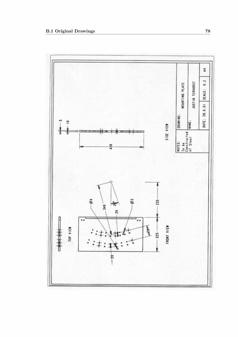
B.1 Original Drawings 78

B.1 Original Drawings 79

B.1 Original Drawings 80
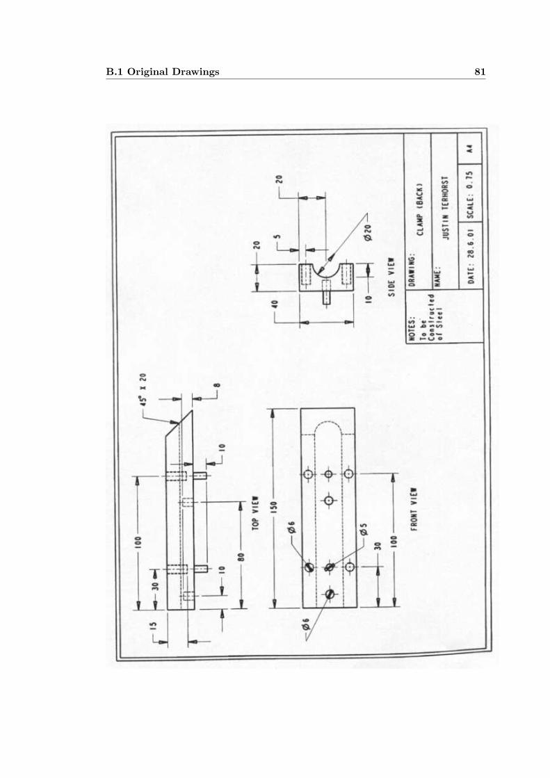
B.1 Original Drawings 81

B.1 Original Drawings 82
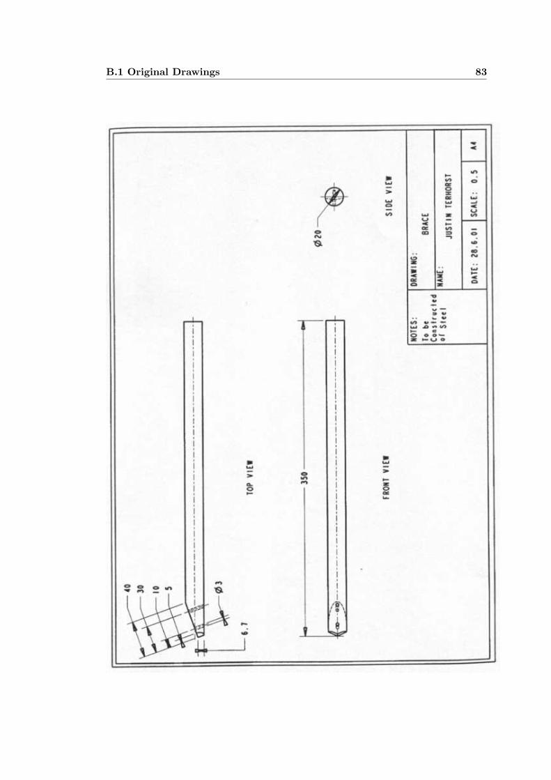
B.1 Original Drawings 83

B.1 Original Drawings 84

B.1 Original Drawings 85

B.1 Original Drawings 86

B.2 Improved component 87
B.2 Improved component
This is the modified I-Beam.

B.2 Improved component 88
Figure B.1: The new I-beam cantilever

Appendix C
Calculations
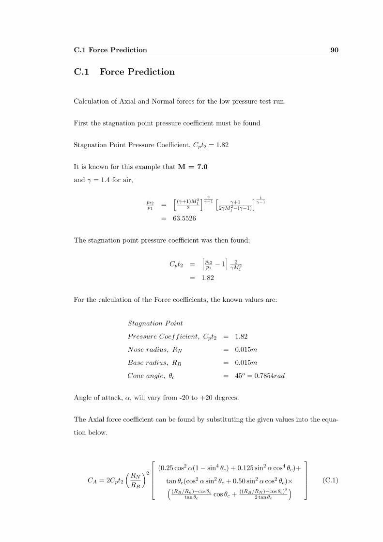
C.1 Force Prediction 90
C.1 Force Prediction
Calculation of Axial and Normal forces for the low pressure test run.
First the stagnation point pressure coefficient must be found
Stagnation Point Pressure Coefficient, Cpt2 = 1.82
It is known for this example that M = 7.0
and γ = 1.4 for air,
pt2
p1=
[(γ+1)M2
12
] γγ−1
[γ+1
2γM21−(γ−1)
] 1γ−1
= 63.5526
The stagnation point pressure coefficient was then found;
Cpt2 =[
pt2
p1− 1
]2
γM21
= 1.82
For the calculation of the Force coefficients, the known values are:
Stagnation Point
Pressure Coefficient, Cpt2 = 1.82
Nose radius, RN = 0.015m
Base radius, RB = 0.015m
Cone angle, θc = 45o = 0.7854rad
Angle of attack, α, will vary from -20 to +20 degrees.
The Axial force coefficient can be found by substituting the given values into the equa-
tion below.
CA = 2Cpt2
(RN
RB
)2
(0.25 cos2 α(1− sin4 θc) + 0.125 sin2 α cos4 θc)+
tan θc(cos2 α sin2 θc + 0.50 sin2 α cos2 θc)×((RB/Rn)−cos θc
tan θccos θc + ((RB/RN )−cos θc)2
2 tan θc
)
(C.1)

C.1 Force Prediction 91
The normal Force can be found by substituting the given forces into the equation below.
CN = 2Cp,t2
(RN
RB
)2
0.25 sinα cosα cos4 θc + sin α cosα sin θc cos θc×((RB/RN )−cos θc
tan θccos θc + ((RB/RN )−cos θc)2
2 tan θc
)
(C.2)
The values for the force coefficients can be seen in the table below. Only angles of
attack of 0 to 20 degrees have been looked at, as the force coefficient of α = −20o
would simply be the negative of α = +20o.
Angle of attack Axial Force Normal Force
(degrees) Coefficient Coefficient
0.0 1.1375 0.0000
2.5 1.1358 0.0297
5.0 1.1308 0.0593
10 1.1109 0.1167
20 1.0340 0.2194
To find the forces the density and velocity in the free stream must be determined. It
has been assumed that the flow that takes place in the Gun Tunnel is isentropic.
Must first find density at stagnation conditions;
To = 750K
Rair = 287
Po = 2.58MPa
(from pressure transducer measurement)
ρo = PoRTo
= 2.58×10⁶
287×750
= 11.986kg/m3
assuming isentropic change,

C.2 frequency prediction calculations 92
ρ0
ρ1= 383.32
ρ1 = 0.031233kg/m3
and
T0T1
= 10.8
T1 = 69.44 K
To find the free stream velocity now,
U1 = M ×√RT1γ
= 7×√287× 69.44× 1.4
= 1169.29m/s
Now the Forces can be determined from using the free stream values just found
FN = CNρ1U21 ΠR2
B (C.3)
FA = CAρ1U21 ΠR2
B (C.4)
The table of calculated forces can be seen below.
Angle of attack Axial Force Normal Force
(degrees) (N) (N)
0.0 34.335 0.000
2.5 34.285 0.898
5.0 34.133 1.789
10 33.532 3.532
20 31.211 6.621
C.2 frequency prediction calculations
This will show how the natural frequency of the cantilever was estimated.

C.2 frequency prediction calculations 93
First though, the section properties of the cantilever must be found. The cross section
of the I-beam cantilever can be seen below.
Figure C.1: Cross section of the I-Beam cantilever
The second moment of Inertia , I
For a rectangle, Ixx = bh3
12
where b = breadth and h = height
For an I-beam of this size,
I = 12×123
12 − 10×83
12
= 1.013× 10⁻⁹m4
= 1301.33mm4
Now that this is known, we can model the model and sting as a mass on a uniformly
loaded beam. This can be seen in figure 5.5.
The values important to this system are.

C.2 frequency prediction calculations 94
Mass of model, M = 0.016 kg
Ealuminium = 7× 10¹⁰Pa
Length of Cantilever, l = 0.047m
Cross− sectional area,Acs = 6.4× 10⁻⁵m2
Density of Aluminium, ρal = 2710kg/m3
Therefore the mass of the cantilever is,
mc = 0.08152 kg
The frequency of the cantilever, w11 is
ω211 = 3.5152
(EIml3
)
= 3.5152(
7×1010×1.013×10−9
0.08152×0.0473
)
= 1.329797× 10+9
The frequency of the model, w22 is;
ω222 = 3.00
(EIMl3
)
= 3.00(
7×1010×1.013×10−9
0.016×0.0473
)
= 1.645065× 10+8
These can then be combined
ω21 = ω2
11ω222
ω211+ω2
22
= (1.329797×10+9)2×(1.645065×10+8)2
(1.329797×10+9)2+(1.645065×10+8)2
= 1.4640× 10+8
ω1 = 12099.4283 rad/s
= 1925.7 Hz
The Natural frequency of the Cantilever mass system was estimated to be 1925.7Hz.

C.3 Calibration 95
C.3 Calibration
This will outline the calibration process by which the sensitivity of the piezoelectric
films was estimated.
The system was calibrated by applying known masses to the end of the cantilever. A
schematic diagram of this can be seen in the figure below. In this figure, the location
of the centres of the piezoelectric films are represented by yellow dots.
Figure C.2: Diagram of calibration setup
The masses that were applied and their corresponding forces are;
Mass Force
(kg) (N)
0.0000 0.000
0.6179 6.061
1.1159 10.95
1.6179 15.87
2.1159 20.76
The 1.1159kg mass will be used as an example of how to determine the strain in the
cantilever.
Will first examine piezoelectric film #1.

C.3 Calibration 96
It can be seen from the figure that the distance from the line of action of the force to
the piezo film is 34.75mm.
d1 = 34.75mm
F = 10.95 N
The bending moment at the centre of piezo 1 is;
M = F × d1
= 10.95× 34.75mm
= 380.40 Nmm
The bending moment can then be used to find the stress at the piezoelectric film.
σ = M×yI
= 380.4×61301.33
= 1.7538 MPa
For Aluminium, E = 7× 10⁴MPa
The relationship between modulus of elasticity (E), stress and strain is;
E = σε
ε = σE
= 1.75387×104
= 2.506× 10−5 = 25.06× 10−6
= 25.06µε
Using the piezoelectric properties of the film which were described in chapter ref{chap:improvement
we can calculate the expected output charge.
Known values: Area of film, Af = 2× 10⁻⁴
Piezoelectric strain constant,C = 69× 10−3
Strain = 25.06× 10⁻⁶

C.4 Calculating the Aerodynamic Force from Measured Strains 97
Charge,Q = 25.06E−6 × 2× 10−4 × 69× 10−3
= 3.458× 10⁻¹⁰ Coulombs
= 0.0138 nC
Assuming the amplifier output is (3.16/3.00)V/nC, this would produce a voltage of
364.24 mV.
The measured value was 322.7 mv (which was not far from expected). This is of no
significance to the calibration but indicates everything is on the right track.
Based on these measurements the sensitivity of the piezoelectric film would be;
Sensitivity = mVµε
= 322.725.06
= 12.88mVµε
This process must be repeated for all of the different masses and both piezoelectric
films. The results of the calibration are summarised in the body of the report.
The sensitivity of piezoelectric film 1 is 13.03 mV/µε.
The sensitivity of piezoelectric film 2 is 9.56 mV/µε
C.4 Calculating the Aerodynamic Force from Measured
Strains
This show the process that was used to calculate the axial forces on the model.
We know that the cross sectional area of the I-beam is 64mm2
For piezo 1 a voltage change of 59.83mV was recorded during the test run.
therefore the strain is;
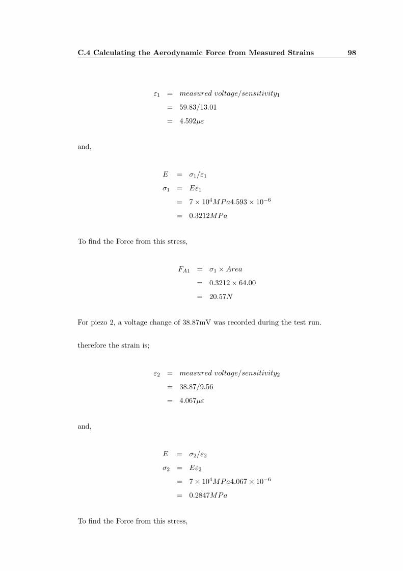
C.4 Calculating the Aerodynamic Force from Measured Strains 98
ε1 = measured voltage/sensitivity1
= 59.83/13.01
= 4.592µε
and,
E = σ1/ε1
σ1 = Eε1
= 7× 10⁴MPa4.593× 10−6
= 0.3212MPa
To find the Force from this stress,
FA1 = σ1 ×Area
= 0.3212× 64.00
= 20.57N
For piezo 2, a voltage change of 38.87mV was recorded during the test run.
therefore the strain is;
ε2 = measured voltage/sensitivity2
= 38.87/9.56
= 4.067µε
and,
E = σ2/ε2
σ2 = Eε2
= 7× 10⁴MPa4.067× 10−6
= 0.2847MPa
To find the Force from this stress,

C.4 Calculating the Aerodynamic Force from Measured Strains 99
FA2 = σ1 ×Area
= 0.2847× 64.00
= 18.22N
The forces found, were: 18.22N and 20.57N. These should be the same, so an average
value will be used.
FA = 19.4N

Appendix D
Source Code

D.1 Loadwavestar2 101
This Appendix contains two matlab scripts
• Loadwavestar2.mat : Used to transform text file from Wavestar to a matrix for
analysis in matlab.
• smo.mat : Used to smooth the raw data that was obtained from the test run.
D.1 Loadwavestar2
This script was written by David Buttsworth.
It allows the data from the oscilloscope that has been saved as a text file by wavestar
to be used in matlab
Inputs: File name, number of rows in text file and number of columns in text file.
Output: Saves the data in a matrix that can be graphed in matlab.
function data=load_wavestar_2(file_name,nrows,ncolumns);
fid=fopen(file_name);
fscanf(fid,’%s’,ncolumns)for i=1:nrows,
ifor j=1:ncolumns,
num1=fscanf(fid,’%f’,1);char1=fscanf(fid,’%s’,1);if char1==’m’,
data(i,j)=num1*1e-3;fscanf(fid,’%s’,1);
elseif char1==’u’,data(i,j)=num1*1e-6;fscanf(fid,’%s’,1);
elseif char1==’n’,data(i,j)=num1*1e-9;fscanf(fid,’%s’,1);
elsedata(i,j)=num1;
endend
end
st=fclose(fid);

D.2 smo 102
D.2 smo
This script was written by Dr David Buttsworth.
This is a moving average filter. At each data point, the data is smoothed over N points
forwards and backwards of that point.
Inputs: Data series and the number of smoothing points (N)
Outputs: Smoothed data series
function new=smo(old,N);%% new=smo(old,N);% Moving average filter. At each point in the% series, the data is smoothed over N points% forwards and backwards of the that point.%% David Buttsworth% October 2002
len=length(old); new=old; for i=1:N,new(1:len-i)=new(1:len-i)+old(1+i:len);new(i+1:len)=new(i+1:len)+old(1:len-i);
end; new=new/(2*N+1);