timberwolf3.2 : al new standard cell placement and global...

TimberWolf3.2 : AL New Standard Cell Placement

and Global Routing Package

Carl Sechen and1 Albert0 Sangiovanni-Vincentelli

Department of EECS Umversity of California

Berkeley. California 94720

Abstract

Timbern-olf3.2 is a new standard cell placement and global routing package. The placement and global routing proceed over 3 distinct stages. The general combinatorial optimization technique known as simulated annealing is used during the first two stages of the placement. In the first stage, TimberWolf3.2 places the cells such that the total estimated interconnect cost is minimized. During the second stage, TimberWolf3.2 iinserts feed through cells as required and the minimization of the total estimated interconnect cost proceeds again in the manner of simulated annealing. The second stage comes to a close following a global routing step. in which the number of wiring tracks needed is accurately estimated. During the third and final stage, local changes are made to the placement whenever such changes result in a reduction in the number of wiring tracks required. TimberWolf3.2 has achieved area savings ranging from 15 to 75% in experiments on numerous industrial circuits.

1. Introduction

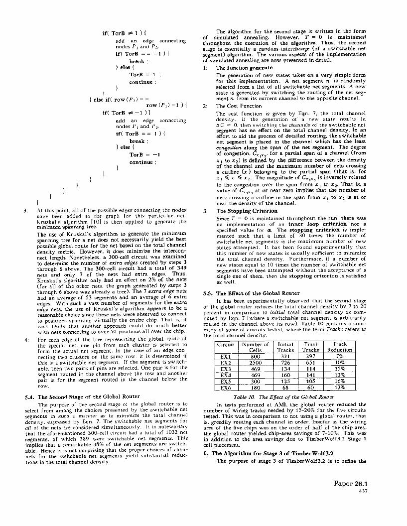
The standard cell layout style is such that the cells are usually arranged in horizontal rows with pads placed around the periphery of the chip. Furthermore, macro blocks may be present on the chip. An example of such a standard cell layout is shown in Fig. 1. The main objectives in standard cell layout are to maximize the performance of the chip (for example. keep- ing the nets as short as possible) and then to minimize the area of the chip. Most of the placement algorithms developed for standard cell placement use aa the objective function the sum of the estimated net lengths. Following the placement. the circuit must then be globally routed in which the ob’ective is to minimize the height of the horizontal channels (’ between the rows>.

Previous placement methodologies were either: (1) h4anual placement. which generally results in area and performance efficiency for small circuits. However, for very large circuits, not only is the design time prohibitively long, but the area and performance suffer. (2) Automatic placement. which has generally resulted in relatively poor area efficiency (in comparison to manual placement) and furthermore, the algorithms used have usually not had the amount of flexibility and extensibility desired by the users.

Extensions and modifications of the general combinatorial optimization technique known as simulat;d annealing [l] were used in an earlier version of TimberWolf. TimberWolfll.0 [2] [3]. in which the above placement drawbacks were addressed. Relatively few global routers for the standard cell layout style have been previously reported.

This paper presents TimberWolf3.2. a new standard cell placement and global routing package. in which numerous algorithmic additions and enhancements were made to the earlier version of TimberWolf1.0. In particular. the standard cell global router is now an integral part of the general placement procedure. Additional flexibilitv was also added to TimberWolf3.2.

The placement ant1 global rourmg now proceed over three dls- tinct stages. In the first stage, TimberWolf3.2 places the cells such that the total estimated interconnect cost is minimized. This stage of the placement is performed using simulated annealing. In the second stage of the placement, TimberWoif3.2 inserts feed-through cells as required and the minimization of the total estimated interconnect cost proceeds again in the manner of simulated annealing. The second stage comes to a close following a global routing step. in which the number of wiring tracks needed is accurately estimated. During the third and final stage. local changes are made to the placement should such a change lead to a reduction in the number of wiring tracks required.

The TimberWolf3.2 package handles standard cell circuit configurations in which the standard cells are arranged in horizontal rows and where as many as 11 macro blocks are permitted on the chip. Furthermore, the pads are placed around the periphery of the chip. Feed through cells are inserted as neces- sary in order to complete the global routing. Furthermore, Tim- berWolf3.2 utilizes uncommitted feed throughs built in to the standard cells whenever possible to avoid the addition of a feed-through cell.

Results on industrial circuits versus numerous automatic and manual layout methods showed that TimberWolf3.2 yielded area savings ranging from 15 to 75%. For all circuits tested, the global router portion of stage 2 reduced the number of wiring tracks needed by an additional 7 to 16% in comparison 6 stage 1 alone. Furthermore, the combination of the nlobal router of stage 2 and stage 3 resulted in wiring track Teductions ranging f;om 15 to 23% in comparison to stage 1 alone. TimberWolf3.2 also features critical-net weighting for performance-driven placement.

- -

The organization of the paper is such that Section 2 briefly reviews the basic simulated annealing algorithm. In Section 3. general TimberWolf3.2 methodology-details are presented. In Section 4. the algorithm for the first stage of the standard cell placement and global routing program is described. Section 5 presents the algorithmic details for stage 2, including the standard cell global router. Next. Section 6 presents the placement-refinement algorithm of stage 3. A summary of the experimental results is presented in Section 7. Finally. Section 8 is devoted to concluding remarks.

2. The Basic Simulated Annealing Algorithm

Simulated annealing has been proposed by Kirkpatrick et al. [l] as an effective method for the determination of global minima of combinatorial optimization problems involving many degrees of freedom. Its basic feature is the possibility of explor- ing the configuration space of the optimization problem allowing hiL2 climbing moves, i.e., the acceptance of new conligurations of the problem which increase the cost. These moves are controlled by a parameter, in analogy with temperature in the annealing process, and are less and less likely towards the end of the process.

Paper 26.1 432

23rd Design Automation Conference

0738-100X/86/0000/0432$01.00 01986 IEEE

Theoretical investigations of the simulated annealing optimization technique have been reported by our research group [4] [S] [6] and elsewhere [7] [g]. The generic structure of the simulated annealin reported earlier [2] f

algorithm as used in TimberWolf3.2 was 31. The following function reviews the gen-

era1 structure of simulated annealing.

AlgorithmStructure( jo *To > f T =T,,: X = jo; whiZe( “stopping criterion” is not satisfied ) {

whiZe( ‘inner loop criterion” is not satisfied > { j = generate{ X > ; if( accept(c(j) .c(X) .T )(

x=j;

cal span of the bounding box of the pins comprising the net. The total estimated interconnect length (TEIL) is quantified by the sum over all nets of the horizontal span plus the vertical span of the net. The total estimated interconnect cost (TEIC) is given by the sum over all nets of: (1) the horizontal span of the net times the horizontal weighting factor for the net, and (2) the vertical span of the net times the vertical weighting factor for the net.

4. The Algorithm for Stage 1 of TimberWolf3.2

This section presents the algorithmic details and results for the first stage of TimberWolf3.2. The purpose of stage 1 is to find a placement of the standard cells such that the TEIC is minimized. A simulated annealing algorithm is employed.

T = update( T > : 1

The acceptance of a new state j is determined by accept, whose structure is shown below.

accept(c(j),c(i).T 11 AC =c(j>-c(i):

; =f( AC .T ); r = random( 0 , 1 ) ; ifC r <y 1 f

returd 1 ) ; ) eke 1

returrd 0 ) : 1

The simulated annealing algorithm described above is characterized by (1) the generation function generate, (2) the acceptance function accept, (3) the updating function update. (4) the inner loop criterion and (5) the stopping criterion. The acceptance function is governed by the function f shown below.

f(Ac.

It is possible to vary the shape of f by adjusting the control parameter T , called temperature. The updating rule for T is given below.

T,,,. = cxt Told > * Told , 0 < Q < 1 TimberWolf3.2 uses several implementations of simulated

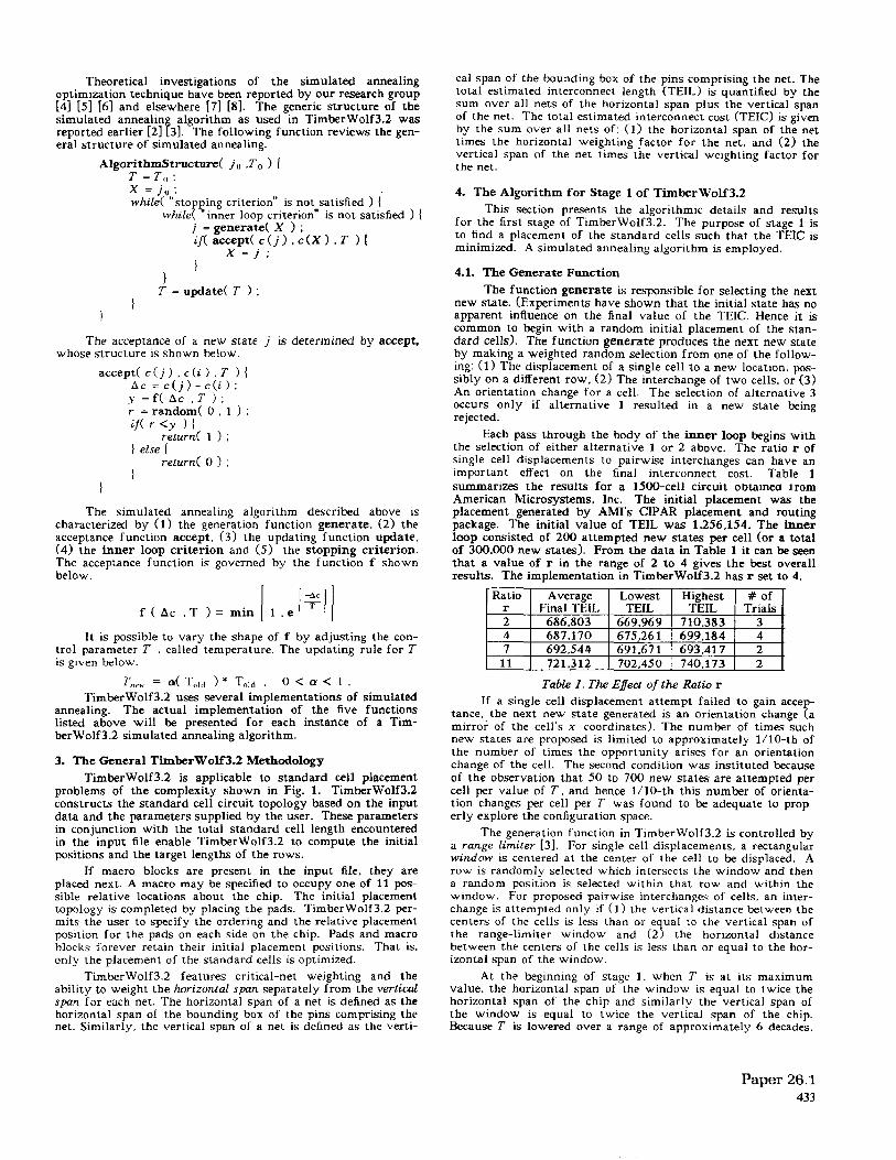
Table 1. The Efect of the Ratio r

annealing. The actual implementation of the five functions listed above will be presented for each instance of a Tim- berWolf3.2 simulated annealing algorithm.

3. The General TimberWolf3.2 Methodology

TimberWolf3.2 is applicable to standard cell placement problems of the complexity shown in Fig. 1. TimberWolf3.2 constructs the standard cell circuit topology based on the input data and the parameters supplied by the user. These parameters in conjunction with the total standard cell length encountered in the input file enable TimberWolf3.2 to compute the initial positions and the target lengths of the rows.

If a single cell displacement attempt failed to gain acceptance, the next new state generated is an orientation change (a mirror of the cell’s x coordinates). The number of times such new states are proposed is limited to approximately l/10-th of the number of times the opportunity arises for an orientation change of the cell. The second condition was instituted because of the observation that 50 to 700 new states are attempted per cell per value of T. and hence l/10-th this number of orientation changes per cell per T was found to be adequate to prop- erly explore the configuration space.

If macro blocks are present in the input file. they are placed next. A macro may be specified to occupy one of 11 possible relative locations about the chip. The initial placement topology is completed by placing the pads. TimberWolf3.2 per- mits the user to specify the ordering and the relative placement position for the pads on each side on the chip. Pads and macro blocks forever retain their initial placement positions. That is. only the placement of the standard cells is optimized.

The generation function in TimberWolf3.2 is controlled by a range limiter [3]. For single cell displacements. a rectangular window is centered at the center of the cell to be displaced. A row is randomly selected which intersects the window and then a random position is selected within that row and within the window. For proposed pairwise interchanges of cells. an interchange is attempted only if (1) the vertical distance between the centers of the cells is less than or equal to the vertical span of the range-limiter window and (2) the horizontal distance between the centers of the cells is less than or equal to the horizontal span of the window.

TimberWolf3.2 features critical-net weighting and the At the beginning of stage 1. when 7’ is at its maximum ability to weight the horizontal span separately from the vertical value, the horizontal span of the window is equal to twice the span for each net. The horizonta1 span of a net is defined as the horizontal span of the bounding box of the pins comprising the

horizontal span of the chip and similarly the vertical span of the window is equal to twice the vertical span of the chip.

net. Similarly, the vertical span of a net is defined as the verti- Because T is lowered over a range of approximately 6 decades,

4.1. The Generate Function

The function generate is responsible for selecting the next new state. (Experiments have shown that the initial state has no apparent influence on the final value of the TEIC. Hence it is common to begin with a random initial placement of the standard cells). The function generate produces the next new state by making a weighted random selection from one of the following: (1) The displacement of a single cell to a new location, pos- sibly on a different row. (2) The interchange of two cells. or (3) An orientation change for a cell. The selection of alternative 3 occurs only if alternative 1 resulted in a new state being rejected.

Each pass through the body of the inner loop begins with the selection of either alternative 1 or 2 above. The ratio r of single cell displacements to pairwise interchanges can have an important effect on the final interconnect cost. Table 1 summarizes the results for a 1500-cell circuit obtamea worn American Microsystems, Inc. The initial placement was the placement generated by AMI’s CIPAR placement and routing package. The initial value of TEIL was 1.256.154. The Inner loop consisted of 200 attempted new states per cell (or a total of 300.000 new states>. From the data in Table 1 it can be seen that a value of r in the range of 2 to 4 gives the best overall results. The implementation in TimberWolf3.2 has r set to 4.

50

Paper 26.1 433

and because it was desired to have the window size shrink slowly, the horizontal and vertical window spans were made proportional to the (base 10) logarithm of the value of T The actual formulae controlling the respective window dimensions are shown below:

windowX 2

= + . xspan loglo( e T 1 (1)

windowY 2

= i . yspan 1ogJ ET 1

windowX where the maximum permitted value of - 1s xspan

and the minimum value for windowX 2

2 was chosen to be 3 (in

the spatial units of the input file).

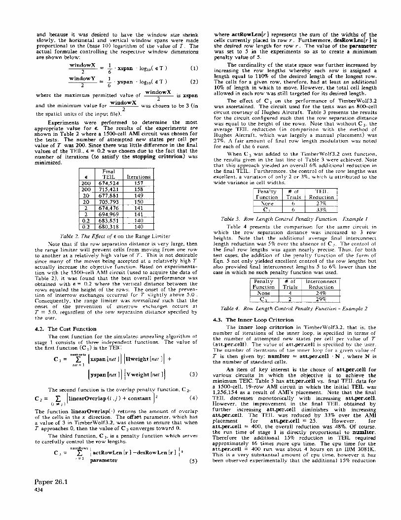
Experiments were performed to determine the most appropriate value for a The results of the experiments are shown in Table 2 where a 1500-cell AMI circuit was chosen for the tests. The number of attempted new states per cell per value of T was 200. Since there was little difference in the final values of the TEIL. E = 0.2 was chosen due to the fact that the number of iterations (to satisfy the stopping criterion) was minimized.

Table 2. The Effecr of E on the Range Limiter

?Gote that if the row separation distance is very large, then the range limiter will prevent cells from moving from one row

to another at a relatively high value of T. This is not desirable since many of the moves being accepted at a relatively high T actually increase the objective function. Based on experimenta- tion with the 1500~cell AM1 circuit (used to acquire the data of Table 2). it was found that the besr overall performance was obtained with c = 0.2 where the verlical distance between the rows equaled the height of the rows. The onset of the preven- rion of interrow exchanges occurred for T slightly above 5.0 Consequently. the range limiter was normalized such that the onset of the prevention of interrow exchanges occurs at T = 5.0. regardless of the row separation distance specified by rhc user.

4.2. The Cost Function

The cost function for the simulated annealing algorithm of stage 1 consists of three independent functions. The value of the first function (C 1) is the TEIC.

C 1 = nlz: [xspn [net I 1 [ Hweight [net ] ] +

I yspan [net I II

Vweight [net I I

The second function is the overlap penalty function, C 2.

C 2 = (4) ( I

5, ) [ linearOverlap (i , j 1 + constant ] *

The function linearOverlap returns the amount of overlap of the cells in the x direction. The offset parameter. which has a value of 3 in TimberWolf3.2. was chosen to ensure that when i” approaches 0, then the value of C 2 converges toward 0.

The third function, Cs. is a penalty function which serves to carefully control the row lengths.

numRows , c3= c

I , actRowLen [r 1 -desRoaLen [r I , *

’ =I parameter (5)

where actRowLen[r] represents the sum of the widths of the cells currently placed in row r Furthermore, desRowLen[r ] is the desired row length for row r . The value of the parameter was set to 5 in the experiments so as to create a minimum penalty value of 5.

The cardinality of the state space was further increased by increasing the row lengths whereby each row is assigned a length equal to 110% of the desired length of the longest row. The cells for a given row. therefore, had at least an additional 10% of length in which to move. However. the total cell length allowed in each row was still targeted for its desired length.

The effect of CJ on the performance of TimberWolf3.2 was ascertained. The circuit used for the tests was an SOO-cell circuit courtesy of Hughes Aircraft. Table 3 presents the results for the circuit configured such that the row separation distance was equal to the height of the rows. Note that without C3, the average TEIL reduction (in comparison with the method of Hughes Aircraft, which was largely a manual placement) was 27%. A fair amount of final row length modulation was noted for each of the 6 runs.

When C3 was added to the TimberWolf3.2 cost function, the results given in the last line ol Table 3 were achieved. Note that this approach yielded an overall 6% additional reduction in the final TEIL. Furthermore. the control of the row lengths was excellent. a variation of only 2 or 3%, which is attributed to the wide variance in cell widths.

# of TEIL Trials Reduction

0 27% 6 33%

Table 3. Row Length Control Penalty Function - Example I

Table 4 presents the comparison for the same circuit in which the row separation distance was increased IO 3 row heights. Note that the additional average final interconnect length reduction was 5% over the absence of C.>. The control of the final row lengths was again nearly precise. Thus. for both test cases. the addition of the penalty function of the form of Eqn. 5 not only yielded excellent control of the row lengths but also provided final interconnect lengths 5 to 6% lower than the case in which no such penalty function was used.

Table 4. Row Length Control Penalty Function - Example 2

4.3. The Inner Loop Criterion

The inner loop criterion in TimberWolf3.2. that is. the number of iterations of the inner loop, is specified in terms of the number of attempted new states per cell per value of T (att.per.cell). The value of att.per.cell is specified by the user. The number of iterations of the inner loop for a given value of T is then given by: numiter = att.per.cell N , where N is the number of standard cells.

An item of key interest is the choice of att.per.cell for various circuits in which the objective is to achieve the minimum TEIC. Table 5 has att.per.cell vs. final TEIL data for a MOO-cell. 19-row AMI circuit in which the initial TEIL was 1.256.154 as a result of AMI’s placement. Note that the final TEIL decreases monotonically with increasing att.per.cell. However. the improvement in the final TEIL obtained by further increasing att.per.cell diminishes with increasing att.per.cell. The TEIL was reduced by 33% over the AMI placement for att.per.celI = 25. However, for att.pez.cell = 400, the overall reduction was 48%. Of course. the run time of stage 1 is directly proportional to numiter. Therefore the additional 15% reduction in TEIL required approximately 16 times more cpu time. The cpu time for the att.per.cell = 400 run was about 4 hours on an IBM 3081K. This is a very substantial amount of cpu time, however it has been observed experimentally that the additional 15% reduction

Paper 26.3 434

in TEIL often yields an additional final chip area reduction much as 10 to 15%. From this standpoint, the additiona time is almost invariably a good trade off.

/ att.oer.cell # of trials Ave. Final

of as .l cpu

Table 5. ,?flect oj att.per.cell on rhe Final TEIL - Example I Table 6 has att.per.cell vs. final TEIL data for an SOO-cell

Hughes Aircraft circuit in which the initial TEIL was 2.408.206 as a result of their manual placement. Again the final TEIL decreases monotonically with increasing att.per.cell. Further- more, it is again observed that the improvement in the final TEIL obtained by further increasing att.per.cell diminishes with increasing att.per.ce.11. The TEIL was reduced by 9% over the Hughes placement for att.per.cell = 100. However, for att.per.cell = 400, the overall reduction was 24%. That is, for a four-fold increase in the cpu time, the final TEIL was reduced an additional 15%.

1 att.Der.cell 1 # of trials 1 Ave. Final [

Table 6. Effect of att.per.cell on the Final TEIL - Example 2

4.4. The Control of T

The function update (T ) is expressed by

T,,,,.. = a( T”,,, ) T,,,# 0 < a < 1 (0) where a versus T,, for the TimberWolf3.2 implementation is shown in Table 7. The entries in the first column indicate the smallest value of T for which the corresponding entry in the second column (a> is valid. That for 40.000 < T < 4.000.000. a is set to O.iZi, for 20.000 < T < 40.000. (I is set to 0.84. and so on. Using the cooling schedule of Table 7, 117 iterations are required to reduce T < 0.1 (that is. to satisfy the stopping criterion) given that the initial value of T = T, = 4.000,OOO.

The strategy used in TimberWolf3.2 was based on the following: (1) Allow 3 to 5 iterations in which virtually every new state was accepted and where T is reduced quite rapidly from iteration to iteration. (2) Having left the high T regime, reduce T in such a manner that AC is approximately the same from iteration to iteration. (3) When T is reduced below 1.5. then reduce T very rapidly so as to firmly converge to a local minimum of the cost function

Table -. The TimberWnlf3.2 Cooling Schedule (Y vs. T

4.5. The Stopping Criterion

The implementarion of the stopping criterion in Tim- berWolf3.2 IS very straight forward. .&s it w-as noted that AC

approaches 0 as T falls below 0.1, TimberWolf3.2 automati- cally terminates its simulated annealing algorithm as soon as an iteration for T < 0.1 was performed.

4.6. The Effects of Net Weighting

The effects of the TimberWolf3.2 net-weighting capability will be demonstrated via some examples. Table 8 has data for an SOO-cell Hughes Aircraft circuit in which the initial estimated interconnect length was i-996.252 as a result of their manual placement. The number of attempted new states per cell per value of T was 400. The third column in the table represents the total number of feed-through cells which had to be added in order to complete the detailed routing. The fourth column represents the horizontal, or x -directed, component of the TEIL (H-TEIL). total estimated horizontal interconnect length. The row separation distance was the same for the three trials shown in the table.

Table 8. Effe~ls of Net Weighting

Note that if the vertical weighting factor is reduced relative to the horizontal weighting factor (row 2 in Table 8) then the H-TEIL is reduced as expected. If a greater percentage of the TEIL is in the vertical direction, as it is for this case. then it would be expected that the number of feed-through cells required would increase. In fact, the second row of Table 8 confirms this. Similarly, if the vertical weighting factor is increased relative to the horizontal weighting factor (row 3 in Table 8) then the H-TEIL is increased as expected. If a smaller percentage of the TEIL is in the vertical direction, as it is for this case. then it would be expected that the number of feed- through cells required would decrease. This again is confirmed by the third row of Table 8.

Hence. there is an inverse relationship between the number of feed-through cells required and the H-TEIL. This can be viewed as a trade off of horizontal chip width (the effect of the feed throughs) versus vertical chip height (the effect of additional wiring in the horizontal channels). As an example, for double-metal technology., most of the required feed-through paths can be accomplished by the use of the built-in feeds of the standard cells. In this case it would be wise to trade off H- TElL for the additional feed-through path requirements. That is. the latter will not increase the chip width for double metal technology and the former will reduce chip height.

Table 9 has data for a 2700-cell, double-metal AMI circuit in which the original chip area was 6912 miZs* as a result of their automatic placement and routing. The row separation distance equaled the height of the rows.

Table 9. Eflects of Net Weighting on a Double Metal Circuit

The entries of Table 9 were obtained with the row separation distance equal to the height of the rows. The first row of Table 9 represents a TimberWolf3.2 placement in which the vertical net weighting factor was 0.10 times the horizontal factor. The chip area reduction was 48%. However. tens of thousands of feed-through paths were required, and not nearly that many built-in feed throughs were available. Consequently. on the order of 10 thousand feed-through cells had to be added, which added a considerable amount to the final chip width. Also, when a feed-through path was required in a row after most of the built-in feed throughs were exhausted for that row. the search for the remaining paths resulted in very long hor-

Paper 26.1 435

izontal wire runs.

The vertical net weighting factor was increased to 0.4 of the horizontal for the next trial as shown in the second row. This relative weighting scheme resulted in a final chip area which was a 63% reduction in comparison to the AM1 placement. For the third trial. the vertical net weighting factor was reduced a bit to 0.3. Note that the final chip area reduction was also more impressive. now 66%.

The final run was repeated with the vertical net weighting factor of 0.3. however, the number of attempted new states per cell per value of T was increased to 800. This resulted in the best placement obtained for this circuit. Note that the final chip area reduction was 70% over the AMI placement and the number of actual feed-through cells which had to be inserted decreased from 13,789 to 1925.

5. The Algorithms for Stage 2 of TimberWolf3.2

This section describes the algorithms for stage 2 of Tim- berWolf3.2. which includes the global router. As ?’ is reduced below To. the standard cells are no longer permitted to switch rows. This is due to the fact that the vertical span of the range limiter window has been reduced to an amount less than the center-to-center spacing between the rows. At this point, the TimberWolf3.2 program enters the first uart of staae 2. which ” continues the simulated annealing portion of the placement methodology.

Before continuing with.the simulated annealing. the feed- through path requirements are ascertained and then (either built-in feeds are selected or actual feed-through cells are inserted to create the required path. Riext. the cells for each row are sorted according to the location of the x-coordinate of their centers. The celis for each row are then re-placed side-by-side starting from the left edge of the respective row.

5.1. Generation of States for Stage 2 Simulated Annealing

routing in the channels. For t‘wo layers 01 mterconnect. the YACRZ channel router [9] consistently routes channels at density or within one track of density. Hence, the minimization of the total channel density results in the minimization of the total number of wiring tracks required.

An internally-connected (electrically-equivalent) group of pins is referred to as a pin cluster. The location of the pin cluster in the n direction is the average of the x locations of the constituent pins. A portion of a net which must connect two pin clusters is referred to as a net segmenr. It often arises that a pin cluster from one cell must. be connected to a pin cluster from another cell on the same row. If each cluster has a pin on the top of the cell as well as a pin on rhe bottom of the cell. then this net segment is defined as being switchable. That is, a switchable net segment can be routed in the channel above the row or in the channel below the row to which the cells belong. The decision as to which channel to route the switchable net segment is based on the minimization of Eqn. 7.

The TimberWolf3.2 global router performs the optimization in two stages. This section presents the details of the algorithm for stage 1. The purpose of this stage is to generate ner segments for each net such thar the total Manhattan interconnect length is minimized. -Also. for switchable net segmenrs. two possible segments are determined. The function row(P 1. where P is a specific pin cluster, returns the row number to which the cluster belongs. Each net is individually subjected to the following four steps (of stage 1).

1: The pin clusters for the net are determined. Furthermore, the average x coordinate of the constituent-pin locations is ascertained for each pin cluster. Next, the pin clusters are sorted by their average x coordinate. and are inserted in a first-in, first-out queue Q.

2: for( : : 1 I TorB = 0 :

The generation of states function (generate) takes on a somewhat different form during stage 2. For every iteration of the inner loop. the following 5 steps are completed: (1) Ran- domlv select a cell A amongst all the standard cells and feed- through cells. (2) The next step is to find the left neighbor. L . of the selected cell (A ) if such a neighbor exists. (3) Next. find the right neighbor, R. of the selecte; cell A if such a neighbor exists. (4) If L is null. then the next new state attempted is an interchange of cells A and R. On the other hand, if R is null, then the next new state attempted is an interchange of cells A and L. If neither L nor R ii null. one of them”is ranaomly selected to be interchanged with A. If this new state is not accepted. then the next new state is generated by inLerchanging A with the other neighbor. (5) The next new state attempted is generated by proposing an orientation change for cell A.

/* Set the top or bottom flag variable TorB to 0. TorB is set to 1 if an edge was formed between pin cluster PI and a pin cluster Pz where row (P,> = row (I”,) + 1. Similarly, TorB is set to -1 if an edge was formed between pin cluster P, and a pin cluster p, where row (P2) = row (P,) -1. */

P1=poplQ); /* Select the leftmost unexamined pin cluster PI by popping the queue Q */

if(Pl== null ){

break : ) else 1

fort ; ; 1 {

5.2. The Cost Function for Stage 2 Simulated Annealing

Since cells do not change rows during stage 2 and since no cell overlapping is ever present during! this stage. the cost function for St&e j simulated annealing is much s<mpler. Th- cost function consists only of the C, term as shown in Eqn. 3 of Section 4.2

5.3. The First Stage of the Global Router

At this point, TimberWolf3.2 has placed rhe standard cells such that a local minimum in the TEIC is achieved. The gaal of the global router is to select pairs of pins for interconnection such that the total number of wiring tracks required (that is. the height of the chip) is minimized. Note that the width of zhe chip 1s largely fixed, insofar as the maximum roe, span is already de&mined. A good approximation of the number of wiring tracks required is the total channel density (tot(,%an- Dens):

Find the nearest pin P2 to the right of P, such that row(P,) is equal to one of the (three) elements in the following set: i row(Pd . row(P,) + 1 , row (PI) -1 1. This is accomplished by

examining (not popping) each remaining element of the queue Q. in order, until either an element is found whose row belongs to the set. or until all remaining elements of the queue have been examined.

if( P, = = null 1 (

break : I else I

if( row (P,) = = row (PII > {

if( TorB = = 0 ) (

connect nodes P, and P, wirh an edge.

totCbanDens = oil L ,sdmsity [ than 1 (7) break ;

where density [ than I is the density of channel than . Note I that the global router described here is applicable to standard 1 else if( row (P,) = = cell circuits which have two layers of interconnect available for row(P1l + 1) 1

Paper 26.1 436

3:

4:

5.4.

if( TorB f 1 ) 1

add an edge connecting nodes PI and Pz. if( TorB == -1 ) {

break : 1 else 1

TorB = 1 :

continue ; I

I 1 else if( row(P2) = =

row (PII -1 > ( if(TorB f-l 11

add an edge connectmg nodes PI and P2.

if( TorB = = 1 > 1

break : 1 else 1

TorB = -1

continue : I

I I ’

I

1

At this point. all of the aossible edges connecting the nodes have been added to tge graph ” for this parlkular net. krruskal‘s algorithm [IO] is then applied to generaLe Ihe minimum spanrim* tree.

The use of Kruskal’s algorithm to generate the minimum spanning tree for a net does not necessarily yield the best possible global route for the net based on the total channel density metric. However. it does minimize the interconnect length. Nonetheless, a 300-cell circuit was examined to determine the number of extra edges created by steps 3 through 6 above. The 300-cell circuit had a total of 349 nets and only 7 of the nets had extra edges. Thus, Kruskal’s algorithm only had an effect on 2% of the nets (for all of the other nets, the graph generated by steps 3 through 6 above was already a tree). The 7 extra edge nets had an average of 53 segments and an average of 6 extra edges. With such a vast number of segments for the enCra edge nets, the use of Kruskal’s algorithm appears to be a reasonable choice since these nets were observed to connect to positions spanning virtually the entire chip. That is. it isn’t likely that another approach could do much better with nets connecting to over 50 positions all over the chip.

For each edge of the tree representing the global route of the specific net, one pin from each cluster is selected to form the actual net segment. In the case of an edge connecting two clusters on the same row. it is determined if this is a switchable net segment. If the segment is switchable. then two pairs of pins are selected. One pair is for the segment routed in the channel above the row and another pair is for the segment routed in the channel below the row.

The Second Stage of the Global Router

The purpose of the second stage of the global router is to select from among the choices presented by the swllchable net segments in such a manner as to minimize the total channel denslry. expressed by Eqn. 7. The switchable net segments for all of the nets are considered simultaneously. It is noteworthy that the aforementioned 300-cell circuit had a total of 1032 net segments, of which 389 were switchable net segments. This implies that a remarkable 38% of the net segments are switchable. Hence it is not surprising that the proper choices of channels for the switchable net segments yield substantial reductions in the total channel density.

The algorithm for the second stage is written in the form of simulated annealing. However, T = 0 is maintained throughout the execution of the algorithm. Thus, the second stage is essentially a random-interchange (of a switchable net segment) algorithm. The various aspects of the implementation of simulated annealing are now presented in detail.

1: The function generate The generation of new states takes on a very simple form for this implementation. A net segment n is randomly selected from a list of all switchable net segments. A new state is generated by switching the routing of the net segment n from its current channel to the opposite channel.

2: The Cost Function

The cost function is given by Eqn. 7. the total channel density. If the generation of a new state results in AC = 0. then switching the channels of the switchable net segment has no effect on the total channel density. In an effort to aid the process of detailed routing, the switchable net segment is placed in the channel which has the least congestion along the span of the net segment. The degree of congestion. C, Ix 2, for a partial span of a channel (from x 1 to x 2) is defined by the difference between the density of the channel and the maximum number of nets crossing a cutline (n) belonging to the partial span (that is. for x L d x d x2. The magnitude of C,,,* is inversely related to the congestion over the span from x 1 to x2. That is. a value of C, 1X ? at or near zero implies that the number of nets crossing a cutline in the span from x1 to x2 is at or near the density of the channel.

3: The Stopping Criterion Since T = 0 is maintained throughout the run. there was no implementation of an inner loop criterion nor a specified value for a. The stopping criterion is imple- mented such that a limit of 30 times the number of switchable net segments is the maximum number of new states attempted. It has been found experimentally that this number of new states is usually sufficient to minimize the total channel density. Furthermore, if a number of new states equal to 10 times the number of switchable net segments have been attempted without the acceptance of a single one of them, then the stopping criterion is satisfied as well.

55. The Effect of the Global Router

It has been experimentally observed that the second stage of the global router reduces the total channel density by 7 to 20 percent in comparison to inizial total channel density as com- puted by Eqn. 7 (where a switchable net segment is arbitrarily routed in the channel above its row). Table 10 contains a summary of some of circuits tested, where the term Tracks refers to the total channel density.

Table IO. The Effect of the Global Router

In tests performed at AMI. the global router reduced the number of wiring tracks needed by 15-20s for the five circuits tested. This was in comparison to not using a global router. that is. greedily routing each channel in order. Insofar as the wiring area of the five chips was on the order of half of the chip area. the global router yielded chip-area savings of 7-100/c. This was in addition to the area savings due to TimberWolf3.2 Stage 1 cell placement.

6. The Algorithm for Stage 3 of TimberWolf3.2 The purpose of stage 3 of TimberWolf3.2 is to refine the

Paper 26.1 43-l

standard cell placement such that the total channel density is minimized. A simulated annealing type algorithm is usszd for stage 3. However. note that at the end of stage 2 of Tim- berwolf. T has been reduced to nearly zero. Consequently. T = 0 is maintained throughout the stage 3 simulated annealing algorithm.

The generation of states function (generate) has a form which is identical to the function generate of stage 2. That is, randomly selected cells are interchanged with their neighboring cells and the effect on the total channel density is noted. If the change in the total channel density is less than or equal to 0, then the new state is retained. Similarly, new states are generated by mirroring cell’s x coordinates. Again. if the change in the total channel density is less than or equal to 0. then the new state is retained.

The cost function is again given by Eqn. 7,. the total channel density. For‘each new state generated. the nets connected to the cell or cells involved in the new sZate generation must be completely re-global routed. These nets must be subjected to stage 1 of the global router. All of the nets of the circuit are then subjected to stage 2 of the global router. where the optimum choice of channel is made for each switchable net segment. Note that nets other than those subjected to stage I must be re-subjected to stage 2 since many of them had their positions chosen based on the positions of the moved nets.

The stopping criterion for stage 2 of the global router is altered somewhat. In particular, a limit of 5 times the number of switchable net segments is the maximum number of new states attempted for stage 2 of the global router. Furthermore. if a number of new states equal to 1.5 times the number of switchable net segments have been atlempted without the acceptance of a single one of them. then the stopping criterion is satisfied as well.

After the conclusion of the second stage of the global router. the new value of the total channel density is compared to the previous value. If the new value is less than or equal to the previous, then the interchange of cells or cell orientaLion change is accepted.

6.1. Other Simulated Annealing Details

Since T = 0 is maintained throughout stage 3 of Tim- berWolf3.2. no implementation of an inner loop criterion nor a specified value for CY. The stopping criterion is satisfied if a number of new states equal to a user-supplied parameter times the number of standard cells and feed-through cells have been attempted without having observed a reduction in the total channel density. From experiments conducted on stage 3 of TimberWolf3.2. a parameter value of 2.0 appears to minimize the total channel density.

6.2. The Effect of Stage 3 of TimberWolf3.2

It has been experimentally observed that stage 3 of Tim- berWolf3.2 reduces the total channel density by 4 to 15 percent in comparison to rhe total channel densIt:, at the end of stage 2 of TimberWolf3.2 (thal IS. followInS the optimued global routing of the TimberWolf3.2 placement achieved by mimmiza- tion of the total estimated interconnect cost). Table 11 contains a summary of some of the circuits tested. where the term Tmcks refers to the total channel density. The user-supplied parameter for the stopping criterion was 2.0 for the examples shown in the table. It is apparent from the table that the reduction in the total channel density as a result of stage 3 is quite substantial.

Initial Circuit Number of Tracks Final Track

Cells after Tracks 1 Reduction

Table Il. The Effect of Stage 3 of TimberWdf3.1?

7. Summary of the Experimental Results

The performance of the TimberWolf3.2 standard cell placement and global routing package was compared to several existing industrial .and commercially available packages. including comparisons to manual placements. The initial testing was accomplished with the aid of an interface to the CIPAR standard cell placement and routing package developed by AMI. Comparisons of sta e 1 of TimberWolf3.2 with CIPAR were published earlier [21 31 B

7.1. TimberWolf3.2 Comparisons with the Global Router

Later tests were performed using both stages 1 and 2 of TimberWolf3.2. The global router portion of TlmberU’olf3.2 was also interfaced to the CIPAR placement and rouling package developed by AMI. For the largest circuit (2700-cell CktF). the global router reduced the area by another 8% this was achieved after the cell placement based on the minimization of the total estimated interconnect cost. A tolal area savings of 75% was achieved for CktF’ when both the TimberWolf3.2 placement optimization and the global rouler (stages 1 and 2) were applied. The results are summarized in Table 12. showing the additional area reductions due to use of the global router and also the overall area reductions as a result of using both Tim- berWolf3.2 placement and global routing (that is, the use of stages 1 and 2). Note that the cpu time for the global router is quite modest.

-

EL

Global CPU Router Final Time

Circuit # Cells Area Chip Area VAX 780 Reduction Reduction in Mins

CktF 2700 8% 75% 2 CktG 1500 8% 45% 1 CktA 1500 6.1% 34% 1 CktB 1000 6% 35% 0.5 ~

Table 13. Global Router Result Y for A MI Circuit J

7.2. TimberWolf3.2 Comparisons Including Stage 3

The TimberWolf3.2 placement and global routing package was compared with another commercially developed placement

ro ram rd.

which was based. in part, on the min-cut algorithm Two double-metal technology circuits were selected for

comparison. The first consisted of 2500 cells and 2 macro blocks. The second contained 469 cells. The results are shown in Table 13. Note that for the larger (2500-cell) circuit, Tim- berWolf3.2 produced a total channel density which is 36% smaller than that produced by the commercial placement package.. For this circuit. TimberWolf3.2 required 35% fewer feed- through paths. including 75% fewer actual feed-through cells. Furthermore. the TimberWolf3.2 placement had a total estimated interconnect length which was 37% smaller. Tim- berWolf3.2 required approximately 15 hours of cpu time on an IBM 3081); to achieve the results for the larger circuit shown in Table 13.

For the smaller (46!J-cell) circuit. TimberWolf3.2 produced a total channel density which is 23% smaller rhan that produced by the commercial placement package. l:or this circuit, Timber1Volf3.2 required 18% fewer feed-through paths. including a 100% reduction in the actual feed-through cells required. Furthermore, the TlmberWolf3.2 placement had a total estimated interconnect length which was 17% smaller. TimberWolf3.2 required less than one hour of CPU time on an IBM 3081K to achieve the results for the smaller circuit shown in Table 13.

8. Conclusions

The TimberWolf3.2 standard cell placement and routing package has been shown to provide substantial chip area savings in comparison to existing standard cell layout methods. Tim- berWolf3.2 is written in the C programming language. The package is currently available through the industrial liason program at the Univ. of California at Berkeley. TimberWolf3.2 is an integral part of the ThunderBird standard cell layout system 1121 which was recently developed at Berkelev. ThunderBird

Paper 26.1 438

combines TimberWolf3.2 with the YACR2 [9] channel router. Future research will be directed towards algorithmic improve- ments which will reduce the run time of the TimberWolf3.2 package. For example, an implementation of a parallel simulated annealing algorithm is being developed.

9. Acknowledgements The authors would like to thank American Microsystems.

IIW.. especially ES. Kirk, for allowing the interf’ace of TimberWolf3.2 to the CIPAR system and for providmg test circuits. The authors would also like to thank Hughes Aircraft Co.. particularly C.P. Hsu, for supplying test circuits. In addition. thanks are extended to Intel Corp.. particularly S. Nachtsheim, for supplying test circuits and for supplying computer time on an IBM 3081K. Finally. the authors would like to thank Cry- stal Semiconductor Corp.. particularly M. Callahan. W. Howard. and D. Gibson. for providing many test circuits. The authors would like to acknowledge the support of the MICRO Project of the State of Calif.. Gould-AMl. and the Hughes Air- craft Co.

Table 13. Results of TimberWolf3.2 vs. Commercial Placement Package

8. References

1. S. Kirkpatrick, C. Geiatt and M. Vecrhi. Optimization by Simulated Annealing, Scienca 220, 4598 (May 13, 1983). 671- 680.

2. C. Sechen and A. Sangiovanni-Vincentelli, The TimberWolf Placement and Routing Package, Proc. 1984 Custom Integrated Circuits Conference, Rochester, New York, May 1984.

3. C. Sechen and A. Sangiovanni-Vincentelli. ‘The TimberWolf Placement and Routing Package, IEEE Journal o./ S&d-State Circuits 20, 2 (April 19851, 510.

4. D. Mitra, F. Romeo and A. Sangiovanni-Vincentelli, Convergence and Finite-Time Behavior of Simulated Annealing, Proc. 24th Conf. on Decision and Control, Ft. Lauderdale. FL.. December 1985.

5. F. Romeo and A. Sangiovanni-Vincentelli, Probabiltiic Hill Climbing Algorithms: Properties and Applications, Computer Sciences Press, Chapel Hill, N.C., 1985.

6. F. Romeo, C. Sechen and A. Sangiovanni-Vincentelli, Simulated Annealing Research at Berkeley, Rot. 1984 IEEE International Conf. on Computer Design, Port Chester, New York, October 1984.

I. D. Geman and S. Geman, Stochastic Relaxation, Gibbs Distributions, and the Bayesian Restoration of Images, IEEE Trans. Pattern AnaZysis and Machine Intelligence 6 (1984), ?21- 741.

a. M. Lundy and A. Mew, Convergence of the Annealing Algorithm, Simulated Annealing Workshop, Yorktown Heights, April 1984.

9. .I. Reed, A. Sangiovanni-Vincentelli and A. Santamauro, A New Symbolic Channel Router: YACR2, IEEE Trans. on CAD 4 (July 1985). 208.

10. J. Kruskal, On the Shortest Spanning Subtree of a Graph and the Traveling Salesman Problem, Proc. Amer. Math SC. 7, 1 (19561, 48-50.

11. B. Kernighan and S. Lin, An Efficient Procedure for Partitioning Graphs, Bell System Technical Journal, February 1970, 291-307.

12. D. Braun, C. Sechen and A. Sangiovanni-Vincentelli, ThunderBird: A Complete Standard-Cell Layout System, Proc. 1986 Custom Inregrated Circuits Conference, Rochester, New York, May 12-14, 1986.

Figure 1. The Generalized Standard Cell Layout Style

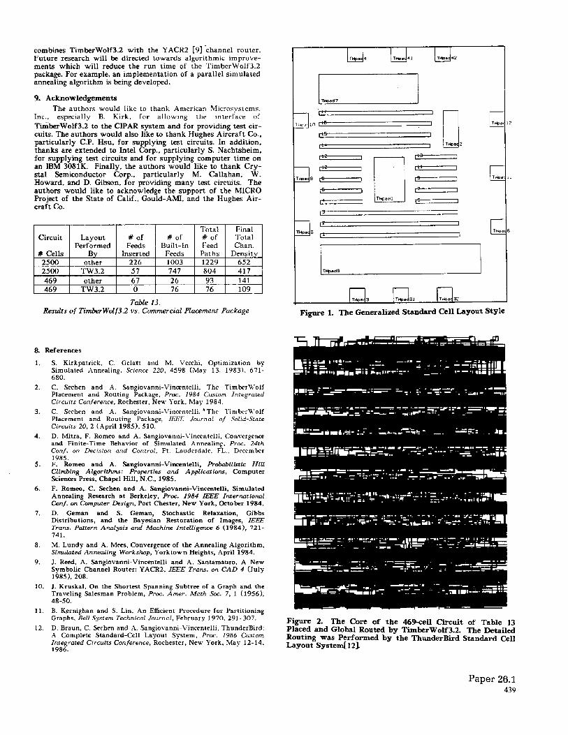
Figure 2. The Core of the 469~~11 Circuit of Table 13 Placed and Global Routed by TimberWolf3.2. The Detailed Routing was Performed by the ThunderBird Standard Cell Layout Systen$lZJ.

Paper 26.1 439

timberwolf3.2 : al new standard cell placement and global...

Documents