TIME AND INCOME IN TRAVEL DEMANDTowards a microeconomic activity framework.

Sergio R. Jara-DíazUniversidad de Chile, Casilla 228-3, Santiago, Chile

Fax (56-2) 6712799 e-mail: jaradiaz@tamarugo.cec.uchile.cl

Abstract

In the first part of this chapter, the microeconomic theory behind discrete mode choice models issummarized, and presently used specifications of modal utility are analyzed with particularemphasis on the role of time and income. Recent theoretical developments are illustrated withempirical results. The framework is then expanded to account for all dimensions of urban travel; todo this, the evolution of time related theories of consumer behavior is synthesized and the need tounderstand travel as part of a general activity framework is highlighted.

TIME AND INCOME IN TRAVEL DEMANDTowards a microeconomic activity framework.

Sergio R. Jara-DíazUniversidad de Chile

1.- INTRODUCTION.

Understanding urban travel demand is nearly like understanding life itself. The day has twenty fourhours, and travel time usually consumes a substantial proportion of the truly uncommitted time. Ingeneral, individuals would rather be doing something else than riding a bus or driving a car, eitherat home, at work, or somewhere else. Accordingly, travelers would like to diminish the number oftrips, to travel to closer destinations and to reduce travel time for a given trip. But such behaviorseems more a consequence than an isolated phenomenon.

On the other hand, most of the relevant characteristics of travelers are obtained through theestimation of discrete choice models within the random utility paradigm. The main objective of thispaper is to summarize the microeconomic foundations of discrete (mode) choice models, withemphasis on the role of time and income. The central idea is to highlight both the genesis andproperties of such models, which means to accept the interpretation of results in terms ofeconomically meaningful constructs as the marginal utility of income or the subjective value of time.This will be shown to have important consequences in the correct specification of such models.

The second objective of the paper is to expand the framework in order to encompass all traveldecisions. To achieve this, the evolution of time related theories of consumer behavior issynthesized; the need to understand travel as part of a general activity framework is highlighted.

2.- DISCRETE CHOICES IN TRAVEL DEMAND.

Disaggregate choice models are the most popular type of travel demand models. The mostimportant element is the (alternative-specific) utility level, usually represented through a linearcombination of cost and characteristics of each alternative, and socio-economic variables for eachgroup of individuals. Under this approach the analyst is assumed to know, for each individual type,which variables determine the level of non-random utility associated to each discrete alternative.This poses many questions regarding model specification: the structure of decisions, thedistribution of the unknown portion of utility, functional form of the observable part, type and formof variables that should be used, and criteria to decide which group of individuals will be regardedas "alike".

The choice of the word utility to describe the equation that represents the level of satisfactionassociated to each alternative, is not casual. It is borrowed from the terminology inmicroeconomics, a discipline that provides a theoretical framework to understand and specifychoice models. The objective in this section is to expose the foundations of this approach in orderto understand the role of income, time, characteristics, preferences, etc. Two caveats should bemade. First, the primary sources of utility will not be examined (i.e. the psychological mechanismsthat make consumption or actions pleasurable). Secondly, and in order to avoid confusion, it isimportant to stress that what is called utility to describe an alternative in discrete choice models, isin fact a conditional indirect utility function that already includes the role of the constraints faced bythe individual as well as a first level of decisions. Thus, although the genesis of direct preferencesare not analyzed, the formation of alternative specific utility levels (e.g. modal) is in the center ofthe following synthesis.

2.1 Quality and income in discrete choice.

The traditional microeconomic framework for consumer's behaviour is stated in terms of a bundleof continuous goods X which are chosen by the individual in an attempt to obtain the maximumlevel of satisfaction, within all possible bundles allowed by his/her purchasing power. After theformalization of Lancaster (1966), who introduced the notion of goods characteristics as theprimary source of utility, the level of satisfaction could be stated in terms of those characteristics(flavor, nutrient, warmth, beauty); accordingly, the problem of choice can be understood properlyaccounting for the fact that characteristics can be obtained through the purchase of market goods,which in turn require money.

There is a relevant type of consumer's decision which can be faced with a slight modification of thepreceding framework: discrete choices. Such a problem arises when the decision to acquire oneunit of a certain generic good (e.g. a car, fruit, a trip) is followed by the choice of a specific type(e.g. a car model, a fruit type, a mode). Then the consumer can be viewed as choosing both theamount of continuous goods and one of the discrete alternatives (mode), each one described by avector jQ containing its qualitative characteristics. Formally (adapting from Mc Fadden, 1981),

an individual is assumed to behave as if

subject to

where Pi and Xi are the price and quantity of good i respectively , jc is the cost of using mode j ,

I is money income and M is the set of alternatives.

x, jjU(X,Q )Max (1)

∑ ≤∈

i i jP X + c I

j M(2)

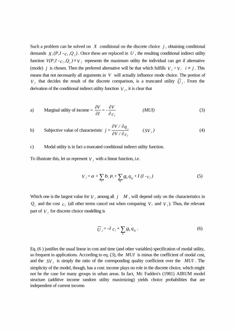
Such a problem can be solved on X conditional on the discrete choice j , obtaining conditionaldemands i j jX (P,I -c ,Q ) . Once these are replaced in U , the resulting conditional indirect utility

function V(P,I -c ,Q ) Vj j j≡ represents the maximum utility the individual can get if alternative

(mode) j is chosen. Then the preferred alternative will be that which fulfills j iV >V i j∀ ≠ . This

means that not necessarily all arguments in V will actually influence mode choice. The portion ofjV that decides the result of the discrete comparison, is a truncated utility jU . From the

derivation of the conditional indirect utility function jV , it is clear that

a) Marginal utility of income = ∂∂

∂∂

VI

= -V

c j

(MUI) (3)

b) Subjective value of characteristic j =V / q

V / cj

j

∂ ∂∂ ∂

(SV )j (4)

c) Modal utility is in fact a truncated conditional indirect utility function.

To illustrate this, let us represent jV with a linear function, i.e.

Which one is the largest value for jV among all j M∈ , will depend only on the characteristics in

jQ and the cost jc (all other terms cancel out when comparing iV and jV ). Thus, the relevant

part of jV for discrete choice modelling is

Eq. (6 ) justifies the usual linear in cost and time (and other variables) specification of modal utility,so frequent in applications. According to eq. (3), the MUI is minus the coefficient of modal cost,and the jSV is simply the ratio of the corresponding quality coefficient over the MUI . The

simplicity of the model, though, has a cost: income plays no role in the discrete choice, which mightnot be the case for many groups in urban areas. In fact, Mc Fadden's (1981) AIRUM modelstructure (additive income random utility maximizing) yields choice probabilities that areindependent of current income.

ji

i ik

k kj jV = + P + q + (I -c )α β γ λ∑ ∑ (5)

j jk

k kjU = - c + qλ γ∑ . (6)

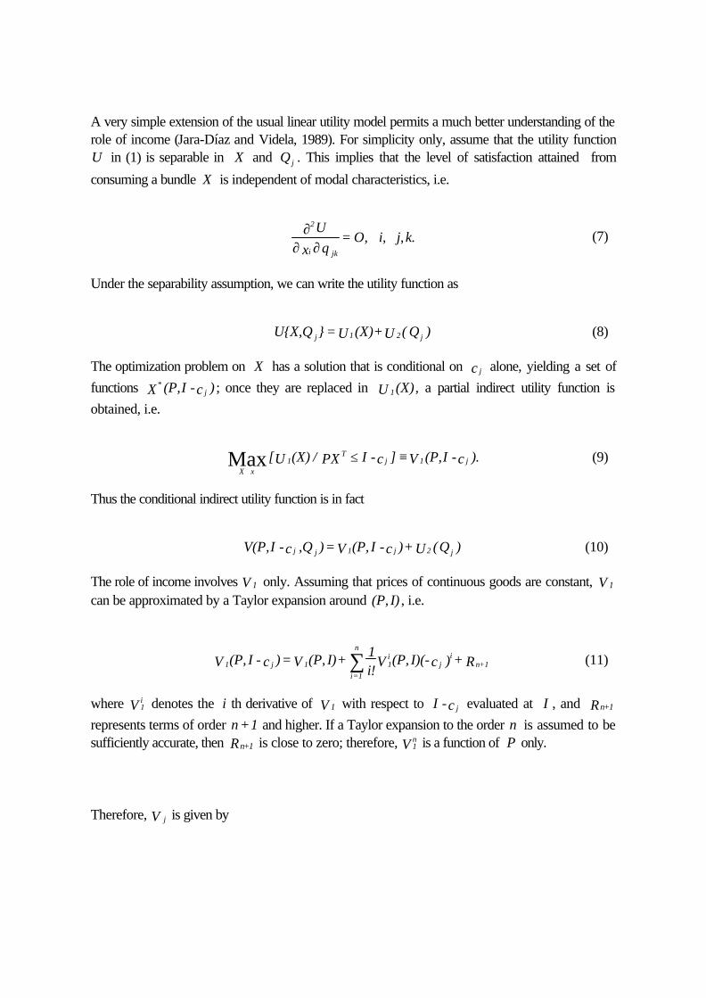
A very simple extension of the usual linear utility model permits a much better understanding of therole of income (Jara-Díaz and Videla, 1989). For simplicity only, assume that the utility functionU in (1) is separable in X and jQ . This implies that the level of satisfaction attained from

consuming a bundle X is independent of modal characteristics, i.e.

Under the separability assumption, we can write the utility function as

The optimization problem on X has a solution that is conditional on jc alone, yielding a set of

functions *jX (P,I -c ) ; once they are replaced in 1U (X), a partial indirect utility function is

obtained, i.e.

Thus the conditional indirect utility function is in fact

The role of income involves 1V only. Assuming that prices of continuous goods are constant, 1Vcan be approximated by a Taylor expansion around (P, I) , i.e.

where 1iV denotes the i th derivative of 1V with respect to I -c j evaluated at I , and n+1R

represents terms of order n+1 and higher. If a Taylor expansion to the order n is assumed to besufficiently accurate, then n+1R is close to zero; therefore, 1

nV is a function of P only.

Therefore, jV is given by

2

i jk

U

x q= O, i, j, k.∂

∂ ∂∀ ∀ (7)

U{X,Q } = U (X)+U ( Q )j 1 2 j (8)

X x1

Tj 1 j[U (X) / PX I -c ] V (P,I -c ).

∈≤ ≡Max (9)

V(P,I -c ,Q )= V (P, I -c )+ U (Q )j j 1 j 2 j (10)

1 j 1i=1

n

1i

ji

n+1V (P, I - c )= V (P, I)+ 1i!

V (P, I)(- c ) + R∑ (11)

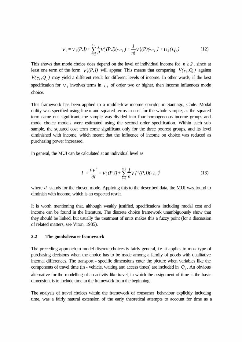
This shows that mode choice does depend on the level of individual income for n 2≥ , since atleast one term of the form 1

iV (P, I) will appear. This means that comparing V(c ,Q )i i against

V(c ,Q )j j may yield a different result for different levels of income. In other words, if the best

specification for jV involves terms in jc of order two or higher, then income influences mode

choice.

This framework has been applied to a middle-low income corridor in Santiago, Chile. Modalutility was specified using linear and squared terms in cost for the whole sample; as the squaredterm came out significant, the sample was divided into four homogeneous income groups andmode choice models were estimated using the second order specification. Within each subsample, the squared cost term come significant only for the three poorest groups, and its leveldiminished with income, which meant that the influence of income on choice was reduced aspurchasing power increased.

In general, the MUI can be calculated at an individual level as

where d stands for the chosen mode. Applying this to the described data, the MUI was found todiminish with income, which is an expected result.

It is worth mentioning that, although weakly justified, specifications including modal cost andincome can be found in the literature. The discrete choice framework unambiguously show thatthey should be linked, but usually the treatment of units makes this a fuzzy point (for a discussionof related matters, see Viton, 1985).

2.2 The goods/leisure framework

The preceding approach to model discrete choices is fairly general, i.e. it applies to most type ofpurchasing decisions when the choice has to be made among a family of goods with qualitativeinternal differences. The transport - specific dimensions enter the picture when variables like thecomponents of travel time (in - vehicle, waiting and access times) are included in jQ . An obvious

alternative for the modelling of an activity like travel, in which the assignment of time is the basicdimension, is to include time in the framework from the beginning.

The analysis of travel choices within the framework of consumer behaviour explicitly includingtime, was a fairly natural extension of the early theoretical attempts to account for time as a

j 1i=1

n-1

1i

ji

1n

jn

2 jV = V (P,I)+ 1i!

V (P,I)(- c ) +1n!

V (P)(- c ) +U (Q )∑ (12)

λ= VI

= V (P,I)+ 1i!

V (P, I)(- c )*

11

i=1

n -1

1i+1

di∂

∂ ∑ (13)

"requisite" for goods consumption (reviewed in the next section). By 1970, Gronau adaptedBecker's (1965) theory to model mode choice including both time and money constraints, showingthat the (discrete) decision depended on something that now we would call modal utility, whichwas a weighted sum of cost and travel time (see Gronau, 1986).

One of the most popular microeconomic approaches specifically aimed at understanding modechoice, some years later introduced modal travel time it and cost ic as variables that influenceutility through the impact on goods consumption G and leisure time L . This goods/leisure trade-off approach (Train and Mc Fadden, 1978) can be summarized as follows, for the case of a singletrip in a given O-D pair

subject to

i M,∈

where W is working time, w is wage rate, E is income from other sources and τ is totalavailable time. By virtue of equation (15), working more (increasing W ) means consuming more(G ) reducing leisure (L ), and vice versa. Thus, the trade-off between goods and leisure issynthesized by W . As in the previous problem, represented by equations (1) and (2), this can besolved in two steps, using W as a "pivot", replacing G and L as functions of W from (15) and(16) in (14 ). Then the optimal value for W can be found conditional on mode choice (i.e. on icand it ), which yields a conditional demand for working time *W as a function of w,E - ci andτ - t i . If this is replaced back in the utility function, a conditional indirect utility iV is obtained.Giving U the Cobb-Douglas form K G L1-β β , the result is

Again, mode choice is decided by comparison among iV , i M∀ ∈ . For a given individual, thisapproach yields choices commanded by the maximum value of -c / w - ti i or -c - wti i .

It should be noted that what we have called the truncated conditional indirect utility function iU , in

the case of equation (17) corresponds to an expression of the form

MaxU(G, L) (14)

G + c = wW + Ei (15)

L+W + t =i τ (16)

i1- 1-

i-

iV = K(1 - ) [w ( - t )+ w (E - c )].β β τβ β β β (17)

i1-

i-

iU = K w t - K w c′ ′β β (18)

which is again linear in cost and time. Note that when β → 0 , then ′K = K and choice isdetermined by -c - wti i ; when β → 1 , then ′K = K and choice follows the maximum of- t - c / wi i . This is the origin of the popular cost over income specification of modal utility, inwhich income is in fact a proxy for the wage rate.

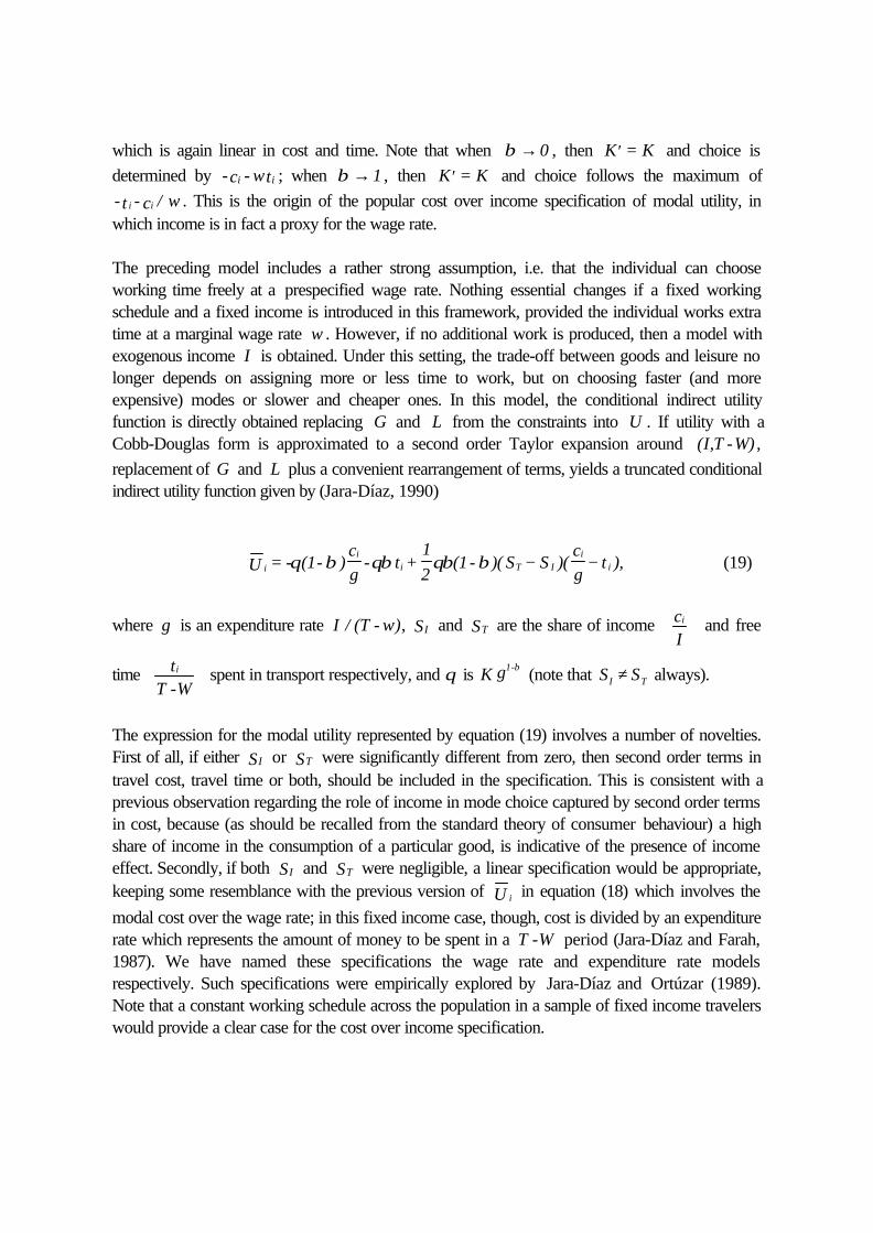
The preceding model includes a rather strong assumption, i.e. that the individual can chooseworking time freely at a prespecified wage rate. Nothing essential changes if a fixed workingschedule and a fixed income is introduced in this framework, provided the individual works extratime at a marginal wage rate w . However, if no additional work is produced, then a model withexogenous income I is obtained. Under this setting, the trade-off between goods and leisure nolonger depends on assigning more or less time to work, but on choosing faster (and moreexpensive) modes or slower and cheaper ones. In this model, the conditional indirect utilityfunction is directly obtained replacing G and L from the constraints into U . If utility with aCobb-Douglas form is approximated to a second order Taylor expansion around (I,T -W) ,replacement of G and L plus a convenient rearrangement of terms, yields a truncated conditionalindirect utility function given by (Jara-Díaz, 1990)

where g is an expenditure rate I / (T - w), IS and TS are the share of income icI

and free

time itT -W

spent in transport respectively, and θ is K g1-β (note that S SI T≠ always).

The expression for the modal utility represented by equation (19) involves a number of novelties.First of all, if either IS or TS were significantly different from zero, then second order terms intravel cost, travel time or both, should be included in the specification. This is consistent with aprevious observation regarding the role of income in mode choice captured by second order termsin cost, because (as should be recalled from the standard theory of consumer behaviour) a highshare of income in the consumption of a particular good, is indicative of the presence of incomeeffect. Secondly, if both IS and TS were negligible, a linear specification would be appropriate,keeping some resemblance with the previous version of iU in equation (18) which involves the

modal cost over the wage rate; in this fixed income case, though, cost is divided by an expenditurerate which represents the amount of money to be spent in a T -W period (Jara-Díaz and Farah,1987). We have named these specifications the wage rate and expenditure rate modelsrespectively. Such specifications were empirically explored by Jara-Díaz and Ortúzar (1989).Note that a constant working schedule across the population in a sample of fixed income travelerswould provide a clear case for the cost over income specification.

ii

i T Ii

iU = - (1- )cg

- t +12

(1- )( S S )(cg

t ),θ β θβ θβ β − − (19)

The generalized expenditure rate model represented by equation (19) helps clarifying an importantpoint regarding the stratification of travelers for model estimation. Imagine that a traditional modechoice model with linear utility is specified with the usual cost over income and time variables;assume as well that individuals in the sample have similar preferences (i.e. same K and β) buttrips involve a variety of travel distances (or travel time). This means that individuals in the samplewould have different values for ST and , therefore, different coefficients for cost and time accordingto eq. (19). Therefore, different linear models should be estimated for individuals traveling shortand long distances. In other words, the sample should be stratified according to distance.

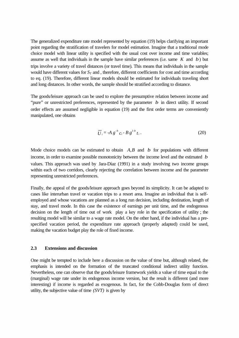
The goods/leisure approach can be used to explore the presumptive relation between income and“pure” or unrestricted preferences, represented by the parameter β in direct utility. If secondorder effects are assumed negligible in equation (19) and the first order terms are convenientlymanipulated, one obtains

Mode choice models can be estimated to obtain A,B and β for populations with differentincome, in order to examine possible monotonicity between the income level and the estimated βvalues. This approach was used by Jara-Díaz (1991) in a study involving two income groupswithin each of two corridors, clearly rejecting the correlation between income and the parameterrepresenting unrestricted preferences.

Finally, the appeal of the goods/leisure approach goes beyond its simplicity. It can be adapted tocases like interurban travel or vacation trips to a resort area. Imagine an individual that is self-employed and whose vacations are planned as a long run decision, including destination, length ofstay, and travel mode. In this case the existence of earnings per unit time, and the endogenousdecision on the length of time out of work play a key role in the specification of utility ; theresulting model will be similar to a wage rate model. On the other hand, if the individual has a pre-specified vacation period, the expenditure rate approach (properly adapted) could be used,making the vacation budget play the role of fixed income.

2.3 Extensions and discussion

One might be tempted to include here a discussion on the value of time but, although related, theemphasis is intended on the formation of the truncated conditional indirect utility function.Nevertheless, one can observe that the goods/leisure framework yields a value of time equal to the(marginal) wage rate under its endogenous income version, but the result is different (and moreinteresting) if income is regarded as exogenous. In fact, for the Cobb-Douglas form of directutility, the subjective value of time (SVT) is given by

i-

i1-

iU = -A g c - B g tβ β . (20)

which is nearly proportional to the expenditure rate when ic and it are negligible compared toincome and leisure time respectively; in fact, to a first order approximation, SVT is equal tog / (1 - )β β from the first part of equation (19). Note that, for a given income level, a person thatworks less has a lower value of time. This explains empirical results like those obtained by Batesand Roberts (1986) regarding the low SVT for retired individuals. Also, note that SVT increaseswith it , which means that the (marginal) subjective valuation of travel time increases with triplength. This is an important point as some claim that one more minute in a short trip should beperceived as more valuable than one more minute in a long one; this fallacy ignores the fact thatwhat is valuable to an individual is leisure time, which is the complement of it . Thus, what mattersis the perception of one minute relative to leisure, which diminishes as leisure increases, orincreases with it .

In applied work, any version of the alternative-specific utility functions introduced here, includesic divided by some form of income (e.g. wage rate, income itself or expenditure rate), all

components of travel time, other (modal) characteristics, socio-economic indexes, etc. Eachvariable has a parameter such that the MUI and jSV are easily calculated using equations (3)

and (4) respectively. As discussed, the SVT under the original version of the goods/leisure trade-off framework is equal to the wage rate, but this is rarely the result in empirical work, in which theratio of the travel time coefficient over the cost/wage coefficient is usually less than one (a resulttheoretically supported by Gronau, 1986). This is related with the formulation of the trade-offmodel, in wich the absolute perception of time is captured by the multiplier of the correspondingconstraint, which is the same for all activities included in L , for work and for travel. Thus, theprice of time is equal for all activities and equal to the wage rate. The case would be different ifrestrictions regarding time were identified beyond equation (16). One possibility is that of minimumtime requirements, like those identified by Truong and Hensher (1985). On the other hand, a ratiosignificantly greater than one has also been obtained (Jara-Díaz and Ortúzar, 1989). In this lattercase, an expenditure rate approach would accept such values as a possibility, as shown inequation (21), where β β/ (1 - ) can take any positive value within the interval 0 1≤ ≤β . Notethat β represents the importance of time in direct utility, which means that individuals with a largeabsolute perception of time could reveal a high SVT if the fixed income, fixed working schedule,is the relevant one.

So far, it seems as if the main issue for the correct specification of (modal) utility is the role ofincome, its endogeneity or exogeneity, depending on whether paid working hours are decided ornot by the individual. In fact, time plays a key role which will be exposed in the next section.

SVT =1-

I - cT -W - t

i

i

ββ

(21)

3.- FROM CONSUMPTION TO ACTIVITIES: THE HISTORY OF TIMERELATED MICROECONOMIC THEORY.

From a microeconomic viewpoint, modeling urban travel demand means introducing time andspace in consumer theory. For a given location pattern, an individual has to choose what goods tobuy and what activities to perform, potentially including leisure, work and transportation. The roleof time began to be discussed with special emphasis from 1965 to 1972 in the economic literature.The traditional framework to model consumer behaviour sees individuals as trying to achieve thehighest level of satisfaction given the constraints that each one faces. As the level of satisfactionwas assumed to be dependent on the amount of goods consumed only, the natural constraint wasthat of a limited purchasing power. The need to understand the labor market made it mandatory tointroduce time as an important element in that framework, as the consumer was assumed to face achoice between work and non-work time. The emphasis, of course, was on the relation betweenwage and the willingness to work (labor supply). In this context, an activity which is essentiallytime consuming as travel was also of interest. In this section, the consumer theories involving theassignment of time are reviewed and discussed, in order to facilitate the integration between thetheory of urban travel with the general theory of time allocation.

3.1 The allocation of time

Becker (1965 ) brought attention to the fact that market goods X are not consumed as they arebought, but they have to be transformed into "basic commodities" Z , which require time to beprepared. Thus, as satisfaction comes from Z , and each iZ depends upon goods consumption

iX and preparation time iT , then utility should be seen as U(X,T) . In Becker's model, income isessentially an endogenously determined variable, as the individual decides how many hours W towork at a pre-specified wage rate w . Thus, two constraints appear originally in his formulation:the traditional budget constraint which relates expenses in market goods with income wW , and anew time constraint which states that working hours plus

i

iT∑ should be equal to total available

time. However, Becker turns the two constraints into one by noting that "time can be convertedinto goods by using less time at consumption and more at work" (pp. 496-497). The resultingconstraint is stated in money terms where a full price for each generalized good iZ appears; thisfull price encompasses the expenses on the necessary market goods, plus a time cost given by

iwT which represents the value of forgone income, i.e. the amount of money the individual wouldearn if he/she assigned iT to work more (see Table 1). Both Johnson (1966) and Oort (1969)used the new time constraint in order to model and understand trip generation and the role oftravel time respectively; both, however, included work time in utility.

A few years later, DeSerpa (1971) developed a model that resembles Becker's, as both goodsand time are included as arguments in utility; however, the approach features importantdifferences. The first one deals with the inclusion of all time components in the utility function inaddition to goods, particularly working time which was explicitly excluded from the previous

framework. The second difference is the addition of a series of constraints reflecting minimum timerequirements for the consumption of each good. DeSerpa's notation is not the most appropriate,as reflected by the need to introduce a number of observations to explain potential limitations ofthe model (e.g. the concept of pure time commodities, a work commodity, and negative prices).Although he makes no reference to the concept of "basic commodities", consumption time isintroduced in utility together with goods; later on, the consumption of each good is called an"activity". The income and time constraints are presented as independent equations, and the role ofthe minimum required consumption time is highlighted as the source of the positive valuation of areduction in iT only if the corresponding constraint is active, which means that the individualwould have liked to spend less time on it.

The first microeconomic model dealing with activities as a central issue was formulated by Evans(1972). Here, the primary source of satisfaction is the type of activity performed, and its measureis the amount of time iT assigned to that particular activity within a period. Thus, in essence,Evans introduced U(T) as an apparently simple departure from the classical goods consumptionmodel; however, activities are costly because they require goods to be actually performed. Thus,market goods are inputs which are necessary to develop activities and, in turn, goods are thesource of the activity cost. What DeSerpa had called pure time activities are allowed to exist inEvans framework simply as a particular case; their cost can be either positive (the individual pays)or negative (the individual is paid). If Q is a matrix containing the input of goods at a certain rateper unit time which are required for each activity, then QT is the vector of goods that has to bebought in order to be able to do the activities contained in T . Thus, the budget constraint is in factrelated to QT . On the other hand, activities will be interdependent in general. This is taken intoaccount by Evans introducing a matrix J that represents links among activity times.

The relation X = QT is the first explicit introduction of a transformation function that turnsactivities into goods and viceversa, which was implicitly expressed both in Becker’s model (the

ijb coefficients in Table 1) and in DeSerpa’s (the ia coefficients). For Evans, the amount of time

to be assigned to each activity is the basic variable, the source of direct utility and the originalsource of both expenses and income. Accordingly, his model is stated in terms of the vector Tonly, as shown in Table 1. For completeness, it should be mentioned that Michael and Becker(1973) further elaborated on the role of the "household production function" Z(X,T) , alongdifferent lines.

3.2 Discussion

As seen, time evolved in consumption theory from a secondary role to a central one in a shortperiod. However, today the basic approach to model consumer behaviour still rests on the idea ofgoods consumption as the primary source of direct utility. From our brief account, though, it seemsthat the fundamental role assigned by Evans to activity time allocation generates a more generaland meaningful framework. If one looks at Table 1 trying to make a synthesis, there are three key

issues to discuss. The first one is the relation between goods and time. Such a relation is fairlygeneral in both Becker’s and Evans’ models through a matrix of fixed coefficients ( ijb in the first

one and Q in the second). The second issue is the presence (or absence) of working time W inthe direct utility function. Unlike Becker, who explicitly leave them out, both DeSerpa and Evansinclude working hours as a direct source of utility. This is an important matter, as including workinghours in utility would make Becker’s synthesis of income and time constraints into one, a mistake,because W could not be used as a pivot variable since the utility level would be affected. This isspecifically pointed out by Evans, and it has previously been highlighted by Johnson (1966) andOort (1969) in their independent departures from Becker’s approach. In fact, Evans criticizesboth Johnson and Oort for not introducing other time related restrictions as, for example, minimumtime required to perform an activity (DeSerpa’s model is not mentioned by Evans). If no timerestrictions are accounted for, the value of time would be equal for all activities because time is adjusted accordingly. And this leads to the third issue, which is more ample than specific minimumtime requirements: the interrelation among activities. This is explicit in Evans’ model only, althoughDe Serpa introduces a related idea which, as explained here, is somewhat related to the idea of atransformation function representing the relation between goods and time. This interrelation is thesource of the relative importance of different activities from an analytical viewpoint; as thisdifferential perception of activities is in fact observed, omitting such a constraint would yielderroneous models.

Thus, starting with time as an addition to commodity consumption in the microeconomic theory ofconsumer behaviour, we find an approach like Evans’, which encompasses all dimensions of theproblem. The striking fact is that his model can be stated in terms of activity times only, as shownin Table 1. Can this model be converted into a goods consumption model? It appeared aspossible, according to the conversion of times T into goods X , i.e. T = Q X-1 . But even if this isdone, the two other constraints still remain: the total time constraint, and a set of linked-activitytype constraints. The resulting commodity consumption model is, therefore, a different one.

On the other hand, and with a different purpose, time played a very important role in what today iscalled home economics. In Gronau's (1986) review, the original formulation of Becker's (1965)time allocation model was generalized to include a "work activity" nZ that enters utility directly;furthermore, the conditions for time to be converted into money are unambiguously established(including an endogenous labor supply and no effect of nZ on U ). This analysis is particularlyinteresting, as the iZ 's are clearly associated with activities, which becomes evident not only in thetreatment of work but in an example where a trip is a necessary ingredient in the production of a“visit”. As two modes are assumed available for the trip, that example is illuminating in tworespects: first, a discrete mode choice model is the outcome and, second, Becker's final goods Zare directly defined as activities. It seems like all roads lead to Rome.

An appropriate view of individual behaviour from a microeconomic perspective should rest onactivities as the primary source of utility, a view that has received some support in the economic

behaviour literature within the last decade (e.g. Juster, 1990 ; Winston, 1987). This implieslooking at goods as means that are necessary to actually realize a set of activities. Doing thisrequires the introduction of a conversion or transformation function that turns activity times intogoods and vice versa. A relation among activity times themselves seems to be necessary as well.This means that introducing time in a microeconomic framework goes beyond the addition of atime constraint. Moreover, time should not be seen as the number of minutes necessary to eitherprepare a final good or consume a market commodity; it is the direct source of utility by means ofits assignment to activities. Note that this apparently innocent change of perspective moves thingsin a different direction. First, the primary result of a consumer model would be activity “demand”functions (as opposed to market demands for goods) and, second, if a U(X,T) type of utility wastaken as a correct formulation, an explanation should be given for the presence of X (as opposedto that of T ). Note that one possible explanation would be the qualitative content of a certain typeof activity, i.e. the marginal utility of activity i could be dependent on the type and amount ofgoods used, making 2

i jU / T X∂ ∂ ∂ different from zero; note also that this would depend solely

on the degree of detail used to describe an activity (e.g. dinning versus dinning elegantly).

4.- TOWARDS A SYNTHESIS: A MICROECONOMIC TRAVEL-ACTIVITIESMODEL

So far, the microeconomic basis for discrete choice models has been summarized, and the time-related theories of consumer behavior have been explored and analyzed. Here follows an attemptat a constructive synthesis.

4.1 Travel choice and time allocation theory

In their original form, both the goods/leisure approach (Train and McFadden, 1978) and Becker'stime allocation model yield the same value of time: the wage rate. This should be no surprise, as inboth cases three conditions concur : income is endogenously determined by freely choosingworking hours, these do not affect direct utility, and no constraints besides income and timebudgets are included. Although they look different and their utilities have different foundations,both models are in fact conceptually the same; it should be recalled, however, that X and T inBecker's model are the inputs to obtain the basic commodities Z , and both are vectors , asopposed to G and L in Train and McFadden's, which are aggregates.

The preceding argument makes Gronau's (1986) extension a relevant one, as he includes a workcommodity in the direct utility, as well as a potentially given labor supply, making Becker's modela particular case. By association, a generalized version of the goods/leisure model can beconstructed, simply replacing W in equation (16) by F vW +W representing fixed and variable(endogenously decided) working hours respectively, and putting W = W v and E = I (fixedincome) in equation (15). Such a model still would be lacking work in direct utility. However, both

the wage rate and expenditure rate specifications could be obtained as particular cases, using vWas pivot; if vW results with a positive value, the wage rate approach holds, and a zero value(corner solution) implies an expenditure rate model. Note that the endogeneity of marginal workinghours is something that can be observed.

The literature shows some attempts to formulate and interpret mode choice models according tothe general frameworks previously developed to approach time allocation. One example of this isthe work by Truong and Hensher (1985), later improved by Bates (1987). They try to translateboth Becker's and DeSerpa's general frameworks into (discrete) mode choice formulations. Dueto the presence of DeSerpa's technical constraints regarding minimum time requirements, theyshow that the conditional indirect (modal) utility should have a mode-specific time coefficient; thiscoefficient should be generic if mode choice was derived from Becker's framework. Thisdifference is also influenced by the fact that travel time does not enter direct utility in the so-calledBecker type model, while it does appear explicitly in DeSerpa's counterpart. In both cases theTHB formulation follows the goods-leisure approach which, as we have seen, is in fact Becker's.However, as goods and "activities" in DeSerpa's are also vectors explicitly written as such, asworking time is not adjustable, and as additional time constraints appear, interpreting DeSerpa'sutility arguments X and T as goods and leisure seems a misuse.

In the preceding paragraphs, the possibility of both building a more general framework for traveldecisions and linking this with the theories of time allocation, has been highlighted. But there is abasic issue to be solved: the arguments in direct utility. Here, the so-called "final commodities" Zseems more an excuse to plug X and T in utility than anything else. In fact, Z is never definedwith enough precision with the exception of Gronau (1986), who eventually calls them "activities".On the other hand, Evans (1972) argues in favour of time devoted to activities as the basicquantifiable source of utility.

For Becker, T is time to prepare the final commodities (which is the reason why W is left out ofutility); for DeSerpa, T is consumption time; for Train and McFadden, the aggregate source ofutility is leisure; Truong and Hensher include travel time in direct utility in the so-called DeSerpamodel. As particularly emphasized by Evans (1972), Bates (1987) and Gronau (1986), includingor not an activity time in direct utility plays a key role in the interpretation of a model. In analyticalterms, the behavior represented by the corresponding first order conditions for optimality, mightinclude or not include a marginal utility of time assigned to the particular activity in question. Thebasic point is whether the individual level of satisfaction can change only because of transfersamong leisure, work and travel, through the time constraint with an impact on purchasing power,or also due to direct pleasure or displeasure.

It seems that there has been an emphasis on keeping as arguments in utility only those elementswhich are believed to increase satisfaction (e.g. leisure, goods). Somehow the idea of non-leisureactivities as direct arguments has been postponed, in spite of the previous examples anddiscussions. To test whether a variable should enter U , the problem can be restated as follows: if

everything else is kept constant, would a change in that variable induce a change in satisfaction?Under this question, all variables that act through other variables in U should not belong to U(as, for instance, income). Thus, work and travel time should indeed be included; generically,goods should not, as they require the assignment of time to their use. Even if some goods arebought for the pleasure of acquiring, satisfaction is realized in the act of buying; if it is a piece ofart, satisfaction is experienced by the act of admiring or by enhancing an action (either at work orat ease). Thus, all particularly identifiable activities should enter U , as separate entities. The onlyjustification for X in U would be a generic description of the activities (e.g. having a morecomfortable bed increases the satisfaction of sleeping as a grossly described activity).

In short, what to use as an argument in direct utility, what constraints should be considered, andwhat is fixed or what is variable, are key decisions to propose a framework aimed at the modellingand understanding of travel decisions. The elements of the problem have been explored, and theyseem to be enough to make a concrete proposal.

4.2 A unified model for travel and activities1

After looking at the microeconomics of mode choice models and the time allocation literature, aunified model can be proposed. There are three basic elements. First, the source of utility is thetime devoted to each activity, including all activities (sleep, eat, talk, travel, work, and so on);second, market goods and services are needed to participate in the different activities, and theyare the source of expenses; finally, besides time and income budget constraints, there are objetiverelations among T and X (feasible T for given X , necessary X for given T ), and among the

iT 's themselves (e.g. activities which require other activities).

From the preceding discussion, a model of travel choices can be looked at as a time allocationproblem, recognizing that utility is directly derived from what the individual does (activities) whichrequires goods that are costly. Formally,

subject to

i

i v F

j=1

B

i M

ij ijT W W t =+ + +j

∑ ∑ ∑∈

δ τ (23)

F(X,T,W ,W ,t) 0F r ≥ (24)

1 This section reproduces the essence of the model in Jara-Díaz (1994).

T,W ,{m},BF v

v

U(T,W ,W ,t)Max (22)

i d

id idj=1

B

i M

ij ij F vP X + c = I + wWj

∑∑ ∑ ∑∈

δ (25)

B = B(X) , (26)

where

T : vector of activity times iT in period τt : vector of travel times ijt in period τB : number of trips in period τ

ijδ : 1 if mode i is used in trip j; 0 otherwise.

F : technical transformation function that converts activities into goods andvice versa; it includes the interrelations among activities.

idX : amount of good i bought in zone d in period τidP : price of good i in zone d .

jM : set of modes available for trip j .

In this model, goods can be bought in different locations, at potentially different prices. Asresidence and work places are given, the number of trips is only sensitive to the choice of X , arelation which appears as eq. (26). This can be viewed as the result of a network related sub-problem (e.g. optimal number of trips given X ). Note that the transformation function (24) is notBecker's Z(X,T) , but Evans' implicit functions X -QT = O and ′ ≤J T O .

The given variables are F F ij ij idW ,I ,t ,c , ,Pτ and w , while the decision variables are

{T },{ },{ X },Wi ij id vδ and B . The solution for B is the generation model, the solution for X is

the distribution model, and the solution for δ is the mode choice model. Note that this formulationis not compatible with the goods-leisure framework. As discussed earlier, ∑ iT = L and∑ id idP X = G . Because of the technical relation between goods and activities, there is an implicitrelation between G and L which has a straightforward interpretation : goods consumptionrequire L and vice versa, which is a missing assumption in both Becker and Train - McFaddenmodels.

Let us see how the model develops when analyzing mode choice in the case of one trip k, which isthe prevailing modelling approach in the field. All other trip decisions will be assumed as given, i.e.number of trips B , destinations (which are one of the dimensions in X ), and all other modechoices. The new problem is

X,T,W i MF v 1 ik B

v, k

U(T,W ,W ,t ,....t ,...t )∈

Max (27)

subject to

ii v F

j kj ikT W W t t =∑ + + +∑ +

≠τ (28)

F(X,T,W ,V ,t) 0F r ≥ (29)

∑≠∑i ij k

j ik F vP X + c + c I +W = , (30)

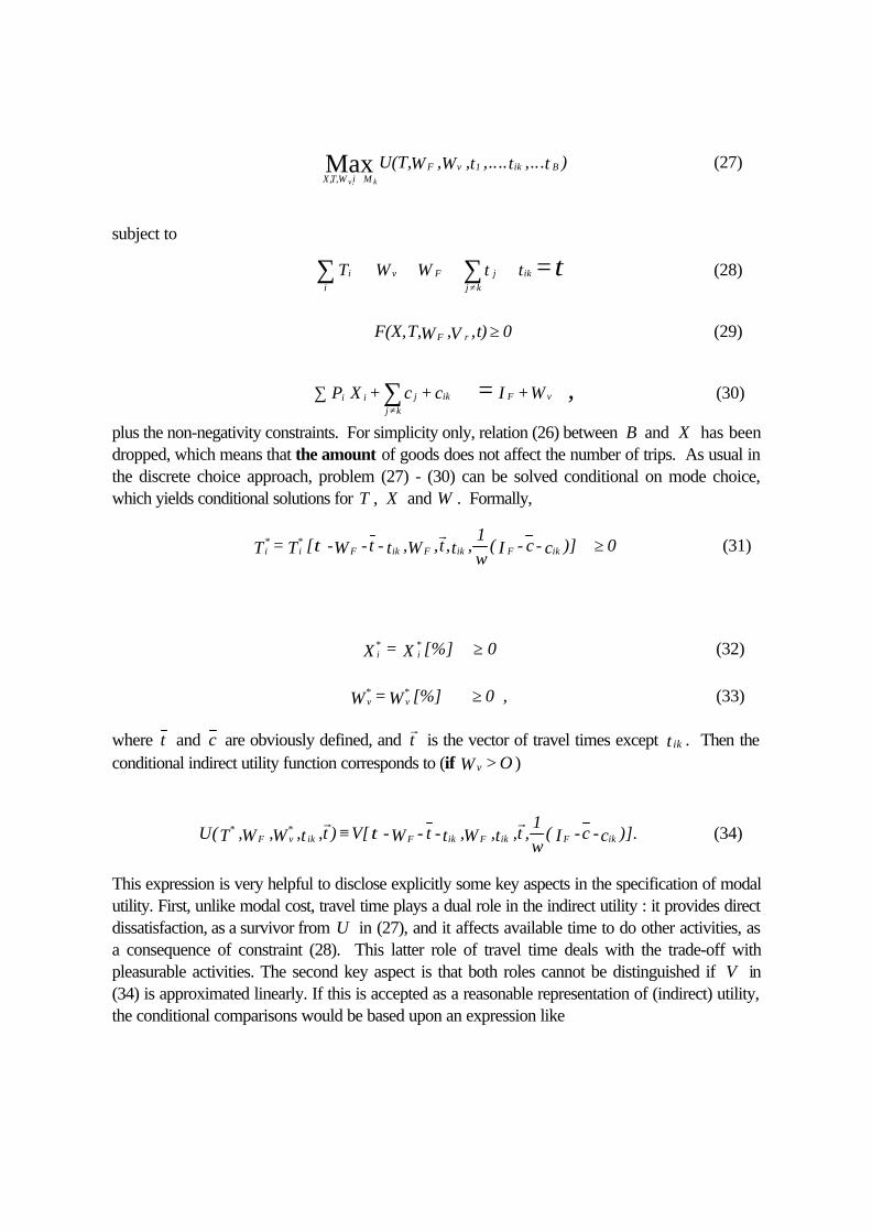
plus the non-negativity constraints. For simplicity only, relation (26) between B and X has beendropped, which means that the amount of goods does not affect the number of trips. As usual inthe discrete choice approach, problem (27) - (30) can be solved conditional on mode choice,which yields conditional solutions for T , X and W . Formally,

where t and c are obviously defined, and rt is the vector of travel times except ikt . Then the

conditional indirect utility function corresponds to (if vW > O )

This expression is very helpful to disclose explicitly some key aspects in the specification of modalutility. First, unlike modal cost, travel time plays a dual role in the indirect utility : it provides directdissatisfaction, as a survivor from U in (27), and it affects available time to do other activities, asa consequence of constraint (28). This latter role of travel time deals with the trade-off withpleasurable activities. The second key aspect is that both roles cannot be distinguished if V in(34) is approximated linearly. If this is accepted as a reasonable representation of (indirect) utility,the conditional comparisons would be based upon an expression like

0[%] X=X *i

*i ≥ (32)

v*

v*W = W [%] 0 ,≥ (33)

i*

i*

F ik F ik F ikT = T [ -W -t - t ,W ,t ,t ,1w

( I - c - c )] 0τr

≥ (31)

U(T ,W ,W ,t ,t ) V[ -W - t - t ,W ,t ,t ,1w

( I -c -c )]. *F v

*ik F ik F ik F ik

r r≡ τ (34)

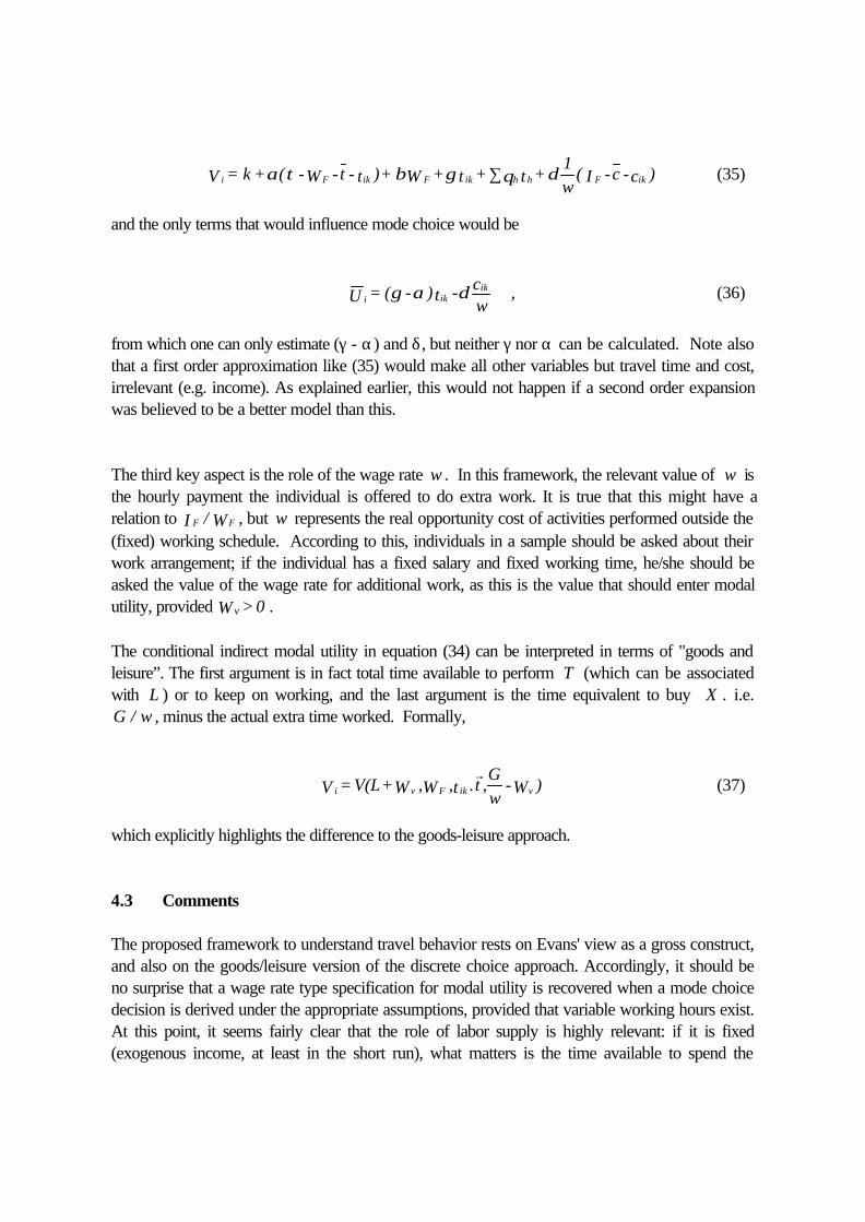
and the only terms that would influence mode choice would be

from which one can only estimate (γ - α) and δ, but neither γ nor α can be calculated. Note alsothat a first order approximation like (35) would make all other variables but travel time and cost,irrelevant (e.g. income). As explained earlier, this would not happen if a second order expansionwas believed to be a better model than this.

The third key aspect is the role of the wage rate w . In this framework, the relevant value of w isthe hourly payment the individual is offered to do extra work. It is true that this might have arelation to F FI / W , but w represents the real opportunity cost of activities performed outside the(fixed) working schedule. According to this, individuals in a sample should be asked about theirwork arrangement; if the individual has a fixed salary and fixed working time, he/she should beasked the value of the wage rate for additional work, as this is the value that should enter modalutility, provided vW > 0 .

The conditional indirect modal utility in equation (34) can be interpreted in terms of "goods andleisure”. The first argument is in fact total time available to perform T (which can be associatedwith L ) or to keep on working, and the last argument is the time equivalent to buy X . i.e.G / w , minus the actual extra time worked. Formally,

which explicitly highlights the difference to the goods-leisure approach.

4.3 Comments

The proposed framework to understand travel behavior rests on Evans' view as a gross construct,and also on the goods/leisure version of the discrete choice approach. Accordingly, it should beno surprise that a wage rate type specification for modal utility is recovered when a mode choicedecision is derived under the appropriate assumptions, provided that variable working hours exist.At this point, it seems fairly clear that the role of labor supply is highly relevant: if it is fixed(exogenous income, at least in the short run), what matters is the time available to spend the

i F ik F ik h h F ikV = k + ( -W -t - t )+ W + t + t +1w

( I -c -c )α τ β γ θ δ∑ (35)

i ikik

U = ( - ) t - cw

,γ α δ (36)

i v F ik vV = V(L+W ,W ,t .t ,Gw

-W )r

(37)

money, while if it is variable (endogenous income), marginal adjustments make the wage rate a keyvariable. Some additional properties of the travel model are

(a) travel and activities time allocation are decisions that pertain to the same class;(b) the interrelations among activities, and those between activities and goods, make it difficult

to accept continuous analytical solutions because of minimum required durations and thepresence of durable goods ;

(c) the subjective value of each activity can be different;(d) if income is relatively small, choices in the time space can be very limited because of the

relations between goods and activities, which can make the time constraint irrelevant ;(e) if income is relatively large, a number of activities are open for consideration because the

necessary goods and services could be acquired. This could make the income constraintirrelevant.

An approach like the one presented here puts the emphasis on time allocation and, therefore, onthe perception of time. The decisions on what to do within a time frame become the relevantphenomenon to investigate. Part of this deals with the analysis of labour supply (how much towork), but understanding individual time allocation as a whole requires a very deep look at humanactivities. Maybe analyzing travel decisions does not require understanding the profound motivesbehind the search for richness, fame or power, but the influence of dominant social values isindeed relevant when studying the structure of daily activities. This should redirect researchtowards the identification of socially induced activities, telecommunication, or the relationsbetween prices and uses of goods (e.g. in addition to the "do I have money" question, add the "doI have extra time to use it", or "what will I stop doing in order to use this"). Thus, acquiring cableTV, having a compact disc player in the car or playing soccer with the neighbors, becomesomething relevant to understand and model. On the other hand, there is a need to understandactivity choice when income is small enough to rule out the acquisition of leisure goods (e.g. toys, gadgets) or the admission to leisure activities (e.g. movies, sports). It might well be that we arefacing the emergence of two social “classes” : those that still have money when the day ends, andthose that still have day when they run out of money.

Needless to say, the aggregate trends on social behaviour, the role of technology and socialvalues, or social idiosyncracy, seem essential to understand travel. Along these lines, the highsubjective valuation of time in Santiago (Chile) previously mentioned, has been examined from theviewpoint of the absolute perception of time. A detailed survey on chilean students showedperceptions which are closer to individuals in the U.S.A. than in Brazil, regarding punctuality,coordination of activities, synchronization, and so on. The conclusion was that the high valuation oftime relative to income revealed by the travel demand models could well be the result of timeperceptions which are highly influenced by the life style in the developed world (Jara-Díaz andRomero, 1992).

The activity-travel framework presented here has also been used to provide a microeconomicbasis to understand residential location (Jara-Díaz, Martínez and Zurita, 1994). One of the nicest

results was the analytical deduction of a term that represents accessibility, associated to eachlocation, which combines the utility obtained from performing activities in different locations withthe generalized cost to reach those places.

5.- CONCLUSIONS.

Consumer theory essentially provides a framework to describe economic behaviour. Within thisframework, the concept of utility function has been instrumental to model demand for goods andservices and to model labour supply. Here, the individual is looked at as if such a function ismaximized. Although travel demand has also benefited from this framework, it seemed necessaryto make a revision of the specific manner in which the general framework has been adapted tounderstand and model urban transport users' behaviour. In this article, travel choices have beenexamined from the perspective of consumer theory, in an attempt to unveil the specific role of thedifferent elements which are part of users' decisions.

Discrete choices, the goods/leisure framework and time related theories of behaviour have beenexposed and examined. From this analysis of the microeconomic foundations of models related totrip decisions, some issues have been clearly established. First is the question about the sources ofdirect utility; starting from goods consumed and going through the concept of basic commodities,consumption time appeared as a necessary item to realize utility. After this modest beginning,time devoted to activities emerged as the basic source of satisfaction, and it is goods that shouldbe looked at as means to an end. Once this is accepted, every single minute in a period should beconsidered. This means, among other things, that both working and travel times are variables thatshould enter utility just as all other activities. Thus, time cannot be converted into money (throughmore work) without altering utility, which makes the fusion of income and time constraints amistake.

On the other hand, the traditional time and income budget constraints are not enough to completethe picture of individual behavior, as market goods and activity times are interrelated (as well asactivities themselves). The addition of a set of technical constraints is necessary to strengthen thefact that certain activities which would be omitted otherwise, are performed. This is a point raisedoriginally by DeSerpa (1971) and Evans (1972), introduced later in the discrete choice literatureby Troung and Hensher (1985). It is a fact, though, that no explicit reference to a transformationfunction has been made so far within the context of mode choice. This needs revision anddiscussions, and Evans' contribution seems to be the best departure point.

It is somewhat surprising to realize that little discussion has taken place regarding the variables indirect utility. In fact, goods and services seemed a reasonable choice until the recognition of a timeconstraint. The introduction of such a constraint implies a relation between goods and activitiesthat cannot be overlooked. Furthermore, once this has been firmly established, identifying theassignment of time to activities as the basic source of satisfaction seems evident. However, thisgives urban travel a different status.

According to Gronau (1986) and Jara-Díaz and Romero (1992), activities related to personalcare (eating, sleeping and other biological needs) consumes in average a little more than elevenhours daily. A normal working schedule would leave something like four hours for discretionaryactivities on a working day. Time assigned to mandatory urban travel can consume a relevant partof this potentially uncommitted time. Thus, understanding travel demand means understandingactivities.

This suggests the convenience of combining the urban travel demand framework with the elementsand analysis of the home economics literature. In fact, in this literature the role of travel has beenhighlighted already. "The shadow price of time affects customer's choice of the optimumcombination of time and market inputs and the decision whether to participate in market work ornot. The imputation of this shadow price is therefore based on the observation of choices wheretime is traded for goods, and the choice concerning labor force participation. Unfortunately, mostoften in situations where goods are traded for time, the amount of time saved is unrecorded"..."One of the few exceptions is the field of transportation " (Gronau, 1986, pp. 292). In this quote,emphasis reveal a goods-leisure point of view; the explanation lies in the type of problemsaddressed in the home economics literature, particularly those pertaining to (domestic) daily life.The individual can make a choice among buying frozen food (which requires a microwave oven),cooking, hiring somebody to cook, or dining out; in essence, this is a choice involving quality,money and... time. And it is true that the trade-offs are difficult to establish because of lack ofrecorded information. It would be desirable indeed to collect and analyze such information inorder to be able to model and understand travel choice as well as goods consumption and activitypatterns.

Although a framework does not necessarily translates immediately into an operational model,implementation should be kept in mind. For example, an activity-travel model as the one proposedhere, yields conditional demands for goods, work and activities as intermediate results whenmodelling mode choice (see eqs. 31 to 33), which turn into unconditional ones if choice isobserved. All variables are potentially known, and a system of equations could be estimated.Undoubtedly, there has been a historical emphasis on market demand for goods, which hasblurred the activity oriented approaches (maybe the present universal trend towards the "I have notime" syndrome, will reverse the situation).

For synthesis, understanding travel behaviour requires understanding the conditions which shapeindividuals' decisions to engage in different patterns of activities. The (relatively new) theory ofhome production should be looked at as belonging to the same family of urban travel theory. Itshould be remembered, though, that economics does not explore the motives behind perceptions;this belongs to the field of psychology.

ACKNOWLEDGEMENTS

This research was partially funded by FONDECYT, Chile. The first version of the activity-travelmodel was presented at the 7th. IATBR Conference in Valle Nevado, Chile (Jara-Díaz, 1994);comments and feedback by the participants are gratefully acknowledged.

REFERENCES

Bates, J.(1987) Measuring travel time values with a discrete choice model : a note. TheEconomic Journal. 97, 493 - 498.

Bates, J.and M. Roberts (1986) Value of time research : summary of methodology and findings. PTRC Summer Annual Meeting.

Becker, G. (1965) A theory of the allocation of time. The Economic Journal 75, 493 - 517.

DeSerpa, A. (1971) A theory of the economics of time. The Economic Journal 81, 828 - 846.

Evans, A. (1972) On the theory of the valuation and allocation of time. Scottish Journal ofPolitical Economy, February, 1-17.

Gronau, R. (1986) Home production - a survey. In Handbook of Labor Economics, Vol. 1, O.Ashenfelter and R. Layard, eds. North Holland, 273 - 304.

Jara-Díaz, S. R, (1990) Valor subjetivo del tiempo y utilidad marginal del ingreso en modelos departición modal. Apuntes de Ingeniería 39, 41 - 50.

Jara-Díaz, S. R, (1991) Income and taste in mode choice models: are they surrogates?Transportation Research 25B, 341 - 350.

Jara-Díaz, S. R, (1994) A general micro-model of users’ behavior: the basic issues. 7th.International Conference on Travel Behavior, Preprints Vol. 1, 91 - 103. Valle Nevado,Chile.

Jara-Díaz, S.R. and M. Farah (1987) Transport demand and user's benefits with fixed income :the goods / leisure trade - off revisited. Transportation Research 21B, 165 - 170.

Jara-Díaz, S. R, F. Martínez and I. Zurita (1994) A microeconomic framework to understandresidential location. Proceedings Seminar H, 22nd. European Transport Forum, U. ofWarwick, 115 - 128.

Jara-Díaz, S. R, and J. de D. Ortúzar (1989) Introducing the expenditure rate in the estimation ofmode choice models. Jornal of Transport Economics and Policy 23, September, 293 - 308.

Jara-Díaz, S.R. and C. Romero (1992) Valoración subjetiva del tiempo: transporte, trabajo yocio en Santiago. En Tecnología y Modernidad en Latinoamérica, E. Sabrovsky, comp.Hachette, Santiago.

Jara-Díaz, S. R. and J. Videla (1989) Detection of income effect in mode choice : theory andapplication. Transportation Research 23B, 393 - 400.

Johnson, B. (1966) Travel time and the price of leisure. Western Economic Journal, Spring,135 - 145.

Juster, F.T. (1990) Rethinking utility theory. The Journal of Behavioral Economics, 19, 155-179.

Lancaster, K. (1966) A new approach to consumer theory. Journal of Political Economy. 74,132 - 157.

McFadden, D. (1981) Econometric models of probabilistic choice. In Structural Analysis ofDiscrete Data with Econometric Applications , C. Manski and D. McFadden, eds. MITPress, Cambridge, MA.

Michael, R, and G. Becker (1973) On the new theory of consumer behavior. Swedish Journalof Economics 75, 378 - 396.

Oort, C. (1969) The evaluation of travelling time. Journal of Transport Economics and Policy,September, 279 - 286.

Train, K. and D. McFadden (1978) The goods / leisure trade-off and disaggregate work tripmode choice models. Transportation Research 12, 349 - 353.

Truong, P. and D. Hensher (1985) Measurement of travel time values and opportunity cost from adiscrete - choice model. The Economic Journal 95, 438 - 451.

Viton, P. (1985) On the interpretation of income variables in discrete choice models. EconomicLetters 17, 203 - 206.

Winston, G.C. (1987) Activity Choice : a new approach to economic behavior. Journal ofEconomic Behavior and Organization 8, 567 - 585.

Table 1. Time related theories of consumer behavior

Framework

ElementTraditional Becker '65 Johnson '66 Oort ’69 De Serpa '71 Evans '72

Utility

Incomeconstraint

Timeconstraint

Technicalconstraint

U(X)

′ ≤P X I

___

___

U[Z(X,T ) ](1)

( )i,j

j ij iP b + T w = w∑ τ

included inincome

implicit inincome

U(B,G,W,L)

G + cB = wW

W + L+ tB =τ

___

U(W,L,tt,I)

I = wW

W + L+ tt =τ

___

U(X,T )(2)

′ ≤P X I

∑ iT =τ

i i iT a X≥

U(T)

′P QT = O

∑ iT =τ

JT O

(X = QT)

≤

(1) T does not include working time(2) X can include “pure time” comodities