time-constrained scheduling of large pipelined datapaths

Journal of Systems Architecture 51 (2005) 665–687

www.elsevier.com/locate/sysarc

Time-constrained scheduling of large pipelined datapaths

Peter Arato, Zoltan Adam Mann *, Andras Orban

Department of Control Engineering and Information Technology, Budapest University of Technology and Economics,

Magyar Tudosok korutja 2., 1117 Budapest, Hungary

Received 23 May 2003; received in revised form 21 May 2004; accepted 17 February 2005

Available online 8 April 2005

Abstract

This paper addresses the most crucial optimization problem of high-level synthesis: scheduling. A formal framework

is described that was tailored specifically for the definition and investigation of the time-constrained scheduling problem

of pipelined datapaths. Theoretical results are presented on the complexity of the problem. Moreover, two new heuristic

algorithms are introduced. The first one is a genetic algorithm, which, unlike previous approaches, searches the space of

schedulings directly. The second algorithm realizes a heuristic search using constraint logic programming methods. The

performance of the proposed algorithms has been evaluated on a set of benchmarks and compared to previous

approaches.

� 2005 Elsevier B.V. All rights reserved.

Keywords: Scheduling; High-level synthesis; Allocation; Pipeline; Genetic algorithm; Constraint logic programming

1. Introduction

In order to cope with the growing complexity ofchip design, high-level synthesis (HLS, [15,6]) has

been proposed, which aims at automatically

designing the optimal hardware structure from

the high-level (yet formal) specification of a sys-

tem. A high-level specification may be e.g. a

1383-7621/$ - see front matter � 2005 Elsevier B.V. All rights reserv

doi:10.1016/j.sysarc.2005.02.001

* Corresponding author.

E-mail addresses: [email protected] (P. Arato), zoltan.

[email protected] (Z. Adam Mann), [email protected]

(A. Orban).

description in a third-generation programming

language such as C or pseudo-code. The optimal-

ity criteria may differ according to the particularapplication. In the time-constrained case, the most

important aspects are: hardware cost, chip size,

heat dissipation, and energy consumption.

We consider pipeline systems which are of great

importance because pipeline processing can boost

the performance of algorithms that are otherwise

difficult to parallelize. For instance in many signal

processing applications pipeline processing is usedto improve the most important performance

measure: throughput.

ed.

mailto:[email protected]

mailto:zoltan. [email protected]



666 P. Arato et al. / Journal of Systems Architecture 51 (2005) 665–687

The previous work on scheduling and allocation

in HLS is reviewed in Section 2. However, the fol-

lowing problems and weaknesses can be identified

in the case of most previous approaches:

• Mostly resource-constrained scheduling has

been addressed. Even in the works that dealt

with time-constrained scheduling, the problem

was often solved by reducing it to a set of

resource-constrained scheduling problems, and

few direct approaches to time-constrained

scheduling have been presented. However,

time-constrained scheduling is very importantfor many real-time applications, in which tim-

ing constraints on latency and/or restart time

are given in advance. Also in hardware–soft-

ware co-design [3,5], which has gained signifi-

cant importance in recent years, the precise

resource constraints on hardware components

are usually not known in advance, but rather

behavioral and time constraints are given.• The complexity of the problem was not studied

formally in most works. This is very important

because there are many different flavors of the

scheduling/allocation problem, some of which

are NP-hard, but some are polynomially solv-

able. Some authors talk about the �NP-hard

nature� of the scheduling problem (e.g. [19]),

but few theoretical contributions have beenmade.

• Also, few efforts have been made to investigate

the complexity of scheduling and allocation sep-

arately. This has lead to the misbelief that allo-

cation is an easy problem and thus it can be

solved as a part of scheduling to calculate the

objective function. However, as it turns out,

allocation is easy only for non-pipeline systems.For pipeline systems, it is NP-hard.

• The algorithms presented in the literature were

tested on graphs with some dozens of vertices.

However, real design problems often consist

of several hundred vertices. This also means

that exact methods are not appropriate for

real-world problems. Generally, the asymptotic

complexity of the presented algorithms was notinvestigated either. From the reported test

results, the behavior of the algorithms on real-

world problems can hardly be inferred.

In this paper, we investigate the problem of

time-constrained scheduling of large datapaths.

Two new scheduling algorithms are presented.The first one is a genetic algorithm (GA),

which—in contrast to previous approaches—is a

direct application of GA to the scheduling prob-

lem, i.e. GA is not only used to generate good

node orders for a list scheduler. The second algo-

rithm is based on constraint logic programming

(CLP), and it is an enhanced list scheduler in

which the trade-off between speed and efficiencycan be tuned. It is different from previously sug-

gested CLP-based methods in that it also specifies

a heuristic search strategy instead of relying on the

built-in exhaustive search of the CLP engine.

We implemented the new algorithms and inte-

grated them into the HLS tool PIPE [6]. Beside

calculating their asymptotic running time, we have

run several empirical tests on large benchmarkproblems. For comparison, an enhanced version

of the force-directed scheduler was also run on

the benchmarks. We chose this modified force-di-

rected scheduler, because it was shown in [6] that

it outperformed other scheduling algorithms that

are suitable for our scheduling model. However,

our tests show that the two new algorithms almost

always produce better results, and often even inshorter running time.

The rest of the paper is organized as follows.

Previous work is presented in Section 2. Section

3 introduces the formal model of the problem

and explains its most important characteristics.

Sections 4 and 5 present the new algorithms. In

Section 6 the empirical evaluation of the new algo-

rithms is described. Section 7 concludes the paper,and the proofs of the theorems can be found in the

appendix.

2. Previous work

In recent years, many scheduling approaches

have been suggested, both optimal and heuristic.Optimal scheduling algorithms have been typically

based on integer linear programming (ILP). For

instance [20] presents an ILP model for resource-

constrained scheduling, but since it takes much

too long to schedule even small graphs with this

P. Arato et al. / Journal of Systems Architecture 51 (2005) 665–687 667

method, it also presents another algorithm, based

on a set of ILP models, that performs significantly

better in practical cases.

Optimal scheduling algorithms based on con-

straint logic programming (CLP) have been sug-gested in [25,29]. These methods make use of a

CLP engine which guarantees that the specified

constraints will be maintained throughout the

search. The search procedure is typically the

built-in branch-and-bound procedure of the CLP

engine, which is a smart, but exhaustive search

strategy. Kuchcinski [25] also supports partial

branch-and-bound.A different optimal method was suggested in

[41], based on bipartite graph matching and

branch-and-bound, for problems that are con-

strained both in time and in resources. This meth-

od was found superior in performance to previous

exact approaches.

Nevertheless, scheduling is NP-hard in general

(the complexity of the problem will be studiedthoroughly in this paper), so that the applicability

of exact scheduling algorithms is restricted to only

small problem instances. In order to handle bigger

problem instances, heuristic scheduling algorithms

have been proposed.

The most popular heuristic schedulers are the

list schedulers because of their low running time.

For instance, Koster and Gerez [22] describe a listscheduler for a scheduling model that is very sim-

ilar to ours. It starts from a set of resources that is

surely a lower bound on the required resources. It

then takes the nodes one after another in a heuris-

tic order, and checks if it can schedule the node

using the given resources. If this is possible, it

schedules the node in the first possible time slot,

and continues. Otherwise it augments the set of re-sources and restarts.

Although list schedulers are fast, they are in

many cases not sufficient because their performance

depends heavily on the node order, and very often

they give disappointing results. Therefore, some

works have tried to use list schedulers together with

another heuristic which aims at finding good node

orders for the list scheduler. Heijligers and Jess[19] investigate such solutions for the time-con-

strained scheduling of non-pipeline systems. It pre-

sents and evaluates four different algorithmvariants

(one of them is taken from [43]), in which the node

order of the list scheduler is optimized using a genet-

ic algorithm. A similar approach is presented in [1],

in which tabu search is used for the optimization of

the node order of the list scheduler.A more complex approach, that is nevertheless

similar in its base idea, is the system in [8,36]. It

deals with the resource-constrained case, what is

more, it assumes that a full description of the tar-

get architecture including available communica-

tion links is known, so that scheduling includes

not only allocation of functional units, but also

that of communication links, as well as messagerouting on the communication links. The solution

is the interplay of three different heuristics: a ge-

netic algorithm optimizes the node order of a gree-

dy scheduler (which is more complex than typical

list schedulers), but the greedy scheduler has only

an abstract, simplified view on the target architec-

ture. The detailed allocation and routing is gener-

ated using a third heuristic, which has all theinformation about the target architecture.

Another popular algorithm is the force-directed

scheduler, which was originally proposed in [35],

and used and enhanced in many later works, e.g.

[32,6,40,2]. Although force-directed scheduling is

just a special list scheduling algorithm, it is much

more complex than standard list schedulers, and

also it has been reported to produce far better re-sults. The force-directed scheduler tries to schedule

approximately the same number of concurrent

nodes for each time cycle, using a probabilistic ap-

proach. It is called force-directed because it always

makes modifications proportional to the deviation

from the optimum, resembling the law of Hooke in

mechanics.

Path-based resource-constrained scheduling ispresented in [30]. This approach takes in each iter-

ation a new path which is not yet fully scheduled,

and schedules it using an algorithm for finding lon-

gest paths in a directed acyclic graph. This method

contains as special case several other algorithms

including list scheduling.

Rotation scheduling [10] is a method for the

minimization of restart time for data flow graphs(DFGs) with loops and inter-iteration dependen-

cies through registers. The main idea of the

algorithm is a technique called retiming, which is


used to move the boundary between iterations.

Using retiming, some intra-iteration dependencies

can be eliminated, which can lead to a shorter

restarting period.

Another interesting approach is described in[37], called rephasing. It aims at decreasing both

latency and area by changing the phase of delay

elements in the control data flow graph (CDFG).

Thus, it is explicitly determined, in which time step

the state variables are refreshed, instead of assum-

ing that each state variable value is available from

the beginning of the iteration, and has to be

refreshed by the end of the iteration.A somewhat different scheduling model is inves-

tigated in [31]. This work aims at improving design

robustness against estimation errors by a special

scheduling approach, called slack-oriented sched-

uling. The slack of a node is the amount of time

by which its duration can increase without violat-

ing consistency constraints. The aim of this work is

to schedule the nodes in such a way that the over-all slack is maximized. Another work to handle

uncertainty in scheduling is presented in [9,42].

However, a completely different solution is given,

based on fuzzy logic. Namely, the duration of

the operations is given as fuzzy numbers, and fuz-

zy operations are used to calculate the sum of the

durations. This fuzzy approach is combined with

rotation scheduling to obtain a scheduler thatcan handle imprecise data. Unbounded delay oper-

ations were considered in [23,24].

Another related scheduling model is that of reg-

ister-constrained scheduling [11], which is actually

an enhanced resource-constrained model, which

also takes registers into account, not only func-

tional units. In this case, it makes sense to move

some data from registers to memory, with auto-matically inserting load/store operations.

Scheduling of control-flow intensive applica-

tions is considered in [27]. This approach starts

from a CDFG, and presents a heuristic scheduler

that performs loop unrolling implicitly. Haynal

and Brewer [18] present a method to schedule a

DFG with loops by applying model checking algo-

rithms to find the minimal cycle length. States arerepresented using a reduced ordered binary decision

diagram (ROBDD), taking into account potential

dependencies between subsequent iterations. This

is accomplished by encoding the parity of the itera-

tion for each operation. The edges of the state ma-

chine are marked with the set of operations that can

be executed simultaneously during that state transi-

tion. The task is to find a shortest cycle in this statemachine that executes all operations.

Our previous work includes [28], where the ba-

sic definitions of our HLS model have already

been defined; this paper extends and sometimes

modifies this previous model (e.g. the notion of

allocation has changed). Furthermore, in [4] we

published the first version of our genetic schedul-

ing algorithm. This work can be regarded as anextension of [4]: the genetic algorithm has been im-

proved (e.g. fitness function), another scheduling

algorithm has been invented and a more thorough

comparison has been given.

3. Definitions and notations

In this paper, we use the model of [6], in which

the system is specified with a so-called elementary

operation graph (EOG), which is an attributed

data flow graph. Its nodes represent elementary

operations (EOs). An EO might be e.g. a simple

addition but it might also be a complex function

block. The edges of the EOG represent data

flow—and consequently precedences—betweenthe operations. The system is assumed to work

synchronously and each EO has a given duration

(determined by its type).

A pipeline system is characterized by two num-

bers: latency, denoted by L, is the time needed to

process one data item, while restart time, denoted

by R (also called iteration interval), is the period of

time before a new data item is introduced into thesystem. Generally R 6 L. Thus, non-pipeline sys-

tems can be regarded as a marginal case of pipeline

systems, with R = L. If a large amount of data has

to be processed, then minimizing R at the cost of a

reasonable increase in L or hardware cost is an

important objective of HLS.

In addition to the EOG, the restart time and the

latency are also given as input for HLS in the time-constrained case.Arato et al. [6] describe algorithms

to transform the EOG so that the given time con-

straints can be met. Afterwards, time-constrained


scheduling is performed, i.e. the starting times of the

EOs are determined, and allocation, in which they

are allocated in physical processing units (PUs).

PU types are associated with a cost (whichmay cap-

ture e.g. area, energy consumption etc.), and thecost of the solution is measured by the sum of the

costs of the needed PUs.

To sum up: the used model supports pipeline

operation, multi-cycle operations, weighted costs,

timing constraints specified in advance. Also, mul-

tiple EO types can be mapped to the same PU

type. On the other hand, only datapath synthesis

is considered, i.e. control structures are not sup-ported directly. (For the handling of conditional

branches during datapath synthesis, see [34].)

There is one more important characteristic of

this model that is not present in other scheuduling

models. In order to avoid hazards a priori, it is as-

sumed that an EO has to hold its outputs constant

during the operation of its direct successors (which

might be implicit buffers if no real EO is scheduleddirectly after it). Therefore the busy time of an EO

(i.e. the time it keeps a PU busy) is the sum of its

duration and that of its longest direct successor.

Now these notions will be defined formally.

Definition 1. Let EO_TYPE denote the finite set

of all possible EO types. dur : EO TYPE ! N

specifies the duration of EOs of a given type.

Definition 2. An elementary operation graph (EOG)

is a 4-tuple:EOG = (G, type,L,R), whereG = (V,E)

is a directed acyclic graph (its nodes are EOs, the

edges represent data flow), type: V ! EO_TYPEis a function specifying the types of the EOs, L spec-

ifies the maximal latency of the system, and R is the

restart time. The number of EOs is denoted by n.

Note that Lmust not be smaller than the sum of

the execution times on any execution path from

input to output.

Definition 3. The duration (execution time) of anEO is: d(EO) = dur(type(EO)).

Fig. 1 shows an example EOG calculating the

roots of a quadratic equation. This EOG was gen-erated from the code segment on the right side of

the figure. This example will guide through the

whole article to visualize the used notions. In this

example EO_TYPE = {mul,add, sub,neg, sqrt,div},

and the function dur is specified as in Table 1.

Hence e.g. d(mul1) = 8, d(sub1) = 4 etc.

The following axioms [6] provide a possible

description of the correct operation of the system:

Axiom 1. EOj must not start its operation until all

of its direct predecessors (i.e. all EOis, for which

(EOi,EOj) 2 E), have ended their operation.

Axiom 2. The inputs of EOi must be constant

during the total time of its operation (d(EOi)).

Axiom 3. EOi may change its output during the

total time of its operation (d(EOi)).

Axiom 4. The output of EOi remains constant

from the end of its operation to its next invocation.

We denote the ASAP (as soon as possible) and

ALAP (as late as possible) starting times of the EOsby asap : V ! N and alap : V ! N, respectively.

Definition 4. The mobility domain of an EO is:

mobðEOÞ ¼ ½asapðEOÞ; alapðEOÞ� \N. The start-

ing time of an EO is denoted by s(EO).

The mobility domain is the set of possible start-

ing times from which the scheduler has to choose,

i.e. s(EO) 2 mob(EO).

Now consider again the example of Fig. 1. Boldarrows indicate edges belonging to one of the lon-

gest paths. This implies that the minimum latency

is 42. Assuming that L = 42, the length of the

mobility domain of the nodes on a longest path

is 0, the mobility domain of other nodes are mob

(mul2) = [0,8],mob(mul3) = [0,26], mob(neg1) = [0,

26]. If one increased the latency to L = 42 + d,d 2 N, all mobility domains would increase withd (ASAP will be the same, and ALAP will increase

with d).

Definition 5. A scheduling r assigns to every EOi astarting time sr(EOi) 2 mob(EOi). The EOG

together with the scheduling r is called a scheduled

EOG, denoted by EOGr.

Definition 6. A valid scheduling is a scheduling

that fulfills the above four axioms.

b

mul2

add1

neg1

double a,b,c;

double x1,x2;

x1=(–b–sqrt (b*b–4*a*c)) / (2*a);x2=(–b+sqrt (b*b–4*a*c)) / (2*a);

c

mul4

a

mul1

mul3

const_4const_2

x2

div2

x1

div1

sub1

sqrt1

sub2

Fig. 1. The EOG calculating the roots of a quadratic equation.

Table 1

Example durations

Type Duration

add, sub, neg 4

mul, div 8

sqrt 10


Proposition 1. Not every scheduling is valid.

Proof. In the example of Fig. 1 let L = 43. It can

be easily calculated that mob(mul1) = [0,1] and

mob(mul4) = [8,9]. However, if mul1 were started

in cycle 1 and mul4 were started in cycle 8, this

would violate the axioms, since mul4 needs the

result of mul1. h

Consequently, the starting times of the EOs can-

not be chosen arbitrarily in their mobility domains,

but the axioms have to be assured explicitly.

Remark 1. The scheduling defined by the ASAP

starting times is valid. Similarly, the scheduling

defined by the ALAP starting times is also valid.

Definition 7. Let R denote the set of all schedu-

lings, and R 0 � R the set of all valid schedulings.

Fixing an objective function Obj : R ! R, wecan now define the general scheduling problem:

Definition 8. The General Scheduling Problem

(GSP) consists of finding a valid scheduling r 2 R 0

for a given EOG that maximizes Obj over R 0.

The only remaining question concerning the def-

inition of the scheduling problem is: how to choose

the objective function Obj? The most logical choicewould be: Obj0(r) = �htheminimumnumberofPUs

required torealizeEOGri. (The minus sign is caused

by the fact that GSP tries to maximize Obj.)


Remark 2. It is straight-forward to assign weights

to the PU types, and calculate the weighted sum of

the required PUs. Although our tool supports this,

we present here the theoretical model without

weights for the sake of simplicity.

In the rest of this section we explain why this

obvious choice is inappropriate and find an alter-

native objective function.

Clearly, EOs whose operation does not overlapin time, can be realized in the same PU. This de-

pends on the restart time and the scheduling

(and thus Obj0 is really a function of r). More pre-

cisely it depends on the busy time of each opera-

tion. The consequence of Axioms 2 and 3 is that

if EOj uses the output of EOi, then EOi should

hold its output stable until the finish of EOj, hence

EOi is busy during the whole d(EOi) + d(EOj) per-iod. This can be reduced using a buffer to store the

result of EOi and EOj can read this buffer after-

wards. In this case EOi is busy only in its real oper-

ation time and during the writing of the buffer,

which is considered to be one clock cycle. Note,

that in this case EOi and EOj must not be sched-

uled directly after each other, because the buffer

must be written. To sum up: the busy time is deter-mined by the longest successor scheduled directly

after the EO, which can also be a buffer.

Definition 9. Let Dr(EOi) be the set of directsuccessors of EOi scheduled directly after it, i.e.

Dr(EOi) := {EOj: (EOi,EOj) 2 E and s(EOj) =

s(EOi) + d(EOi)}. The busy time interval of an EO is:

busyðEOiÞ¼

½sðEOiÞ;sðEOiÞþdðEOiÞþ1�

if DrðEOiÞ¼ ;

sðEOiÞ;sðEOiÞþdðEOiÞþ maxDrðEOiÞ

dðEOjÞ� �

otherwise

8>>>>>>><>>>>>>>:

Definition 10. Two closed intervals [x1,y1] and

[x2,y2] intersect modulo R, iff $z1 2 [x1,y1] andz2 2 [x2,y2], such that z1 � z2 (mod R).

Definition 11. Let PU_TYPE denote the finite set

of all possible PU types. j:EO_TYPE ! PU_

TYPE is a function that specifies which PU type

can execute a given EO type.

A PU type might execute different EOs, e.g. an

ALU can realize all the arithmetic operations.

Definition 12. EOi and EOj are called compatible

iff j(type(EOi)) = j(type(EOj)) and busy(EOi) and

busy(EOj) do not intersect modulo R. Otherwise

they are called incompatible (sometimes also called

concurrent).

It can be proven (see [6]) that this is indeed a

compatibility relation, moreover, two EOs can be

realized in the same PU iff they are compatible.

Note that if EOj is started immediately after EOi

has finished, then they are incompatible. Most re-lated works define the compatibility slightly differ-

ently: they use the operation interval instead of the

busy time interval. However, to schedule two

dependent operations directly after each other is

not realistic, because it can cause hazards. In our

approach these hazards are a priori eliminated [6].

Now we are ready to define the allocation prob-

lem formally.

Definition 13. An allocation is a mapping between

the EOs and the PUs so that the PUs are able to

execute the EOs mapped to them and each PU has

at most one EO to execute in each time step.Formally an allocation is a function a : V !PU TYPE �N with the following characteristics:

(i) If a(EOi) = (pu,k), then j(type(EOi)) = pu

(pu 2 PU TYPE; k 2 N).

(ii) If EOi,EOj 2 a�1(pu,k), then busy(EOi) and

busy(EOj) do not intersect modulo R

(pu 2 PU TYPE; k 2 N).

k means the kth copy of the PU.

The aim of allocation is to calculate the mini-mum number of PUs required for a given sche-

dule, i.e. to calculate Obj0 is equal to solving the

allocation problem.

Proposition 2. In the special case when pipelineprocessing is not allowed (R = L), the allocation

problem can be solved in polynomial time.

Proof. Based on EOGr, we can define a new undi-

rected graph G 0 = (V 0,E 0), called the concurrency

graph (or conflict graph) of EOGr. V0 = V, but


the edges have a different meaning: (EOi,EOj) 2 E 0

iff EOi and EOj are incompatible in EOGr.

Let Vt be the set of EOs that can be realized by

PU type t. It can be seen easily that finding a

realization of EOGr[Vt] (the induced subgraph ofEOGr by Vt) corresponds to a vertex coloring of

G 0[Vt]. Consequently, calculating Obj0 in G 0[Vt]

means calculating its chromatic number.

If pipeline processing is not allowed, then G 0[Vt]

is an interval graph, and the chromatic number of

interval graphs can be found in polynomial time

[17]. Clearly, all types can be handled this way,

independently of each other. (However, it is nottrue that G 0 itself would be an interval graph, but

rather a set of interval graphs, between which all

edges are present.) h

Proposition 3. The allocation problem of pipeline

systems is NP-hard, even if only EOGs with a sin-

gle type and no edges are considered.

Proof. Because of pipeline processing, the class of

possible G 0s is not that of interval graphs, but that

of circular arc graphs, for which finding the chro-

matic number is NP-hard. (For a proof, see

[16].) h

Therefore, we settled for another objective func-

tion, namely the number of compatible pairs (i.e.,

the number of edges in the complement of the con-

currency graph). We had two reasons for this: (i)

Calculating the number of compatible pairs

(NCP) is much easier than calculating the number

of required PUs; and (ii) The above two numberscorrelate significantly, i.e. if the NCP is high, this

usually results in a lower number of required PUs.

We have already seen that it is difficult to calcu-

late the number of required PUs. On the other

hand, the CONCHECK algorithm [6] can determine

the compatibility of two EOs in Oð1Þ steps, and

so the NCP of EOGr can be calculated in Oðn2Þtime.

Now we will formally elaborate on claim (ii).

Intuitively it seems to be logical that the chromatic

number of graphs with many edges is higher than

that of graphs with few edges, but this is not

always true. However, it is true in a statistical

sense.

Definition 14. Let Gn;M denote the set of all

graphs with n vertices and M edges. This can be

regarded as a probability space, in which every

graph has the same probability. Gn;p denotes the

set of all graphs with n vertices, provided with thefollowing probability structure: every edge is

present with probability p, independently from

the others.

Definition 15. Let Q be a graph property (that is,

a set of graphs). We say that Q is almost sure with

respect to Gn,p, iff limn!1ProbðG 2 Q j G 2 Gn;pÞ ¼1. (The same notion with respect to Gn,M is simi-larly defined.)

It is known [7], that the chromatic number

vðGÞ ¼ Hn

logdn

� �

is almost sure with respect to Gn,p, where d = 1/(1 � p). Our aim is to reason about Gn,M.

Definition 16. The graph property Q is said to be

convex, iff (G1 2 Q, G2 2 Q, V(G1) = V(G) =

V(G2), E(G1) � E(G) � E(G2)) ) G 2 Q.

It is also known [14] that if Q is almost sure in

Gn;p, and Q is convex, then Q is also almost sure in

Gn;M , where M ¼ p � n2

� �(i.e. the expected num-

ber of edges).

Clearly, the property that ‘‘v(G) equals a given

value’’ is convex, so we can write with the appro-

priate p and M values:

vðGÞ ¼ Hn

logdn

� �¼ H

nln n

ln1

1� M

n

2

!

0BBBBBB@

1CCCCCCA

is almost sure in Gn,M.

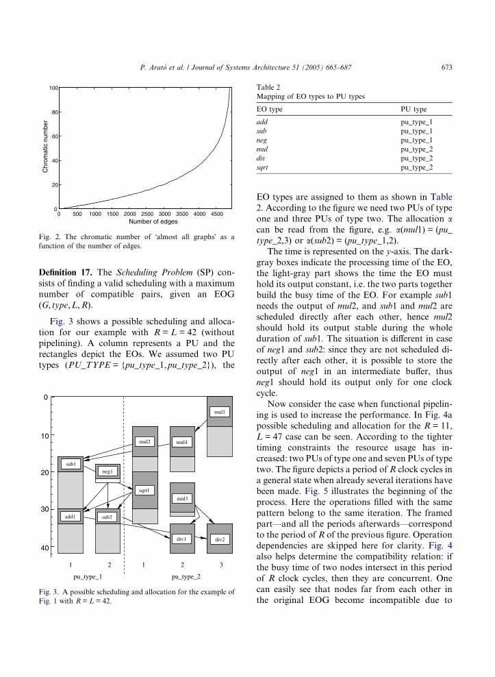
It can be seen easily that this function is monot-

onously increasing in the number of edges. This

can also be seen in Fig. 2 for n = 100.

This shows that maximizing the NCP almost

surely induces solutions requiring fewer PUs.Now we can define the special version of the

above general scheduling problem which we are

concerned with:

0

20

40

60

80

100

0 500 1000 1500 2000 2500 3000 3500 4000 4500

Chr

omat

ic n

umbe

r

Number of edges

Fig. 2. The chromatic number of �almost all graphs� as a

function of the number of edges.

Table 2

Mapping of EO types to PU types

EO type PU type

add pu_type_1

sub pu_type_1

neg pu_type_1

mul pu_type_2

div pu_type_2

sqrt pu_type_2


Definition 17. The Scheduling Problem (SP) con-

sists of finding a valid scheduling with a maximum

number of compatible pairs, given an EOG

(G, type,L,R).

Fig. 3 shows a possible scheduling and alloca-

tion for our example with R = L = 42 (without

pipelining). A column represents a PU and therectangles depict the EOs. We assumed two PU

types (PU_TYPE = {pu_type_1,pu_type_2}), the

0

10

20

30

40

pu_type_1 pu_type_2

sqrt1

mul2 mul4

mul3

div1 div2

mul1

add1

sub1neg1

sub2

2 1 2 31

Fig. 3. A possible scheduling and allocation for the example of

Fig. 1 with R = L = 42.

EO types are assigned to them as shown in Table

2. According to the figure we need two PUs of type

one and three PUs of type two. The allocation acan be read from the figure, e.g. a(mul1) = (pu_

type_2,3) or a(sub2) = (pu_type_1,2).

The time is represented on the y-axis. The dark-

gray boxes indicate the processing time of the EO,

the light-gray part shows the time the EO musthold its output constant, i.e. the two parts together

build the busy time of the EO. For example sub1

needs the output of mul2, and sub1 and mul2 are

scheduled directly after each other, hence mul2

should hold its output stable during the whole

duration of sub1. The situation is different in case

of neg1 and sub2: since they are not scheduled di-

rectly after each other, it is possible to store theoutput of neg1 in an intermediate buffer, thus

neg1 should hold its output only for one clock

cycle.

Now consider the case when functional pipelin-

ing is used to increase the performance. In Fig. 4a

possible scheduling and allocation for the R = 11,

L = 47 case can be seen. According to the tighter

timing constraints the resource usage has in-creased: two PUs of type one and seven PUs of type

two. The figure depicts a period of R clock cycles in

a general state when already several iterations have

been made. Fig. 5 illustrates the beginning of the

process. Here the operations filled with the same

pattern belong to the same iteration. The framed

part—and all the periods afterwards—correspond

to the period of R of the previous figure. Operationdependencies are skipped here for clarity. Fig. 4

also helps determine the compatibility relation: if

the busy time of two nodes intersect in this period

of R clock cycles, then they are concurrent. One

can easily see that nodes far from each other in

the original EOG become incompatible due to

pu_type_1 pu_type_2

0

2

4

6

8

10

1 2 1 2 3 4 5 6 7

mul3

sub2

mul1

sqrt1

mul4

neg1

mul2

sub1

add1

mul4div2 div1mul3

div2 div1

Fig. 4. A possible scheduling and allocation for the example of Fig. 1 with R = 11 and L = 47.


pipelining, e.g. mul1 and div1. Note that to reach a

restart time of 11 clock cycles each operation

should have a busy time not greater than 11, thus

the scheduler did not schedule long dependent

operations after each other, but rather buffers wereinserted between them to reduce the busy time.

Now that we have defined the scheduling prob-

lem, we can present one of the main theoretic con-

tributions of the paper:

Theorem 1. SP is NP-hard.

The proof can be found in Appendix A. This re-

sult shows that it is infeasible to strive for a perfectsolution for large inputs. Rather, we have imple-

mented two different heuristic scheduling methods,

which are presented in the next sections.

4. Genetic scheduling algorithm

In this section we propose an heuristic schedul-ing method based on genetic algorithms [13,21]. In

general, a genetic algorithm starts with an initial

population of individuals representing the (appro-

ximate) solutions of the problem. After that, in

each iteration a new population is generated from

the previous one using the genetic operations:

recombination, mutation and selection. So in each

step there are two populations. The new popula-

tion is first partially filled using recombination

(usually there is a predefined recombination rate,

rr), then the rest using selection. Mutation is then

used on some individuals of the new population(their number is defined by the mutation rate, mr).

The scheduling problem is a good candidate for

applying a genetic algorithm. The applicability of

genetic algorithms requires that the solutions of

the optimization problem can be represented by

means of a vector with meaningful components:

this is the condition for recombination to work

on the actual features of a solution. Fortunately,there is an obvious vector representation in the

case of the scheduling problem: genes are the start-

ing times of the elementary operations. That is, the

individual corresponding to scheduling r is

xr = (sr(EO1), . . . , sr(EOn)).

Identifying the state space is not this straight-

forward. The question is whether non-valid

schedulings should be permitted. Since non-validschedulings cannot be realized, it seems to be log-

ical at first glance to work with valid schedulings

only. Unfortunately, there are two major draw-

backs to this approach. First, this may constrain

efficiency severely. Namely, it may be possible to

get from a valid individual to a much better valid

individual by genetic operations through a couple

Fig. 5. The first couple of iterations for the schedule of Fig. 4.


of non-valid individuals, whereas it may not be

possible, or perhaps only in much more steps to

get to it through valid ones only. In such a case,

if non-valid individuals are not permitted, onewould hardly arrive to the good solution. An

example for such a situation is shown in Appendix

B.

The other problem is that it is hard to guarantee

that genetic operations do not generate non-valid

individuals even from valid ones. This holds for

both mutation and recombination. Thus, if non-

valid individuals are not permitted, the recombina-tion operation cannot be used in the form of cross-

over. Rather, it should be defined as averaging.

But this method does not help to maintain variety

in the population so it can cause degeneration. In

the case of mutation it seems that the only way

to guarantee validity is to immediately get rid of

occasional invalid mutants. However, this would

contradict the principle of giving every individualthe possibility to propagate its characteristics.

For these reasons we decided to permit any

individual (between ASAP and ALAP) in the pop-

ulation, not only valid ones. That is, the state

space is fðx1; . . . ; xnÞ 2 Nn : asapi 6 xi 6 alapi ð16 i 6 nÞg and the population always contains N

such individuals. Of course the scheduler must

produce a valid scheduling at the end. In orderto guarantee this, there must be valid individuals

in the initial population and the fitness function

must be chosen in such a way that it punishes

invalidity. Moreover, the best-so-far valid schedul-

ing is also stored separately, and can be returned at

any time.

Remark 3. Because of the above problems, it was

stated in [8] that genetic algorithms cannot be

applied directly to scheduling. However, as can be

seen, this is indeed possible.

If only valid individuals were allowed, the fit-

ness would be equal to NCP. Since non-valid indi-

viduals are also allowed, but they should be

motivated to be less and less invalid, the fitness

has a second component (beside NCP), which isa measure of invalidity, namely the number of col-

lisions (NoC), i.e. the number of precedence rules

(edges of the EOG) that are corrupted. So the fit-

ness is monotonously increasing in the number of

compatible pairs and monotonously decreasing in

the number of collisions. In choosing the appropri-

ate fitness function one can have two different

strategies:1. To motivate the individuals towards validity

has the highest priority, i.e. any increase in NCP

cannot compensate the smallest increase in NoC.

This strategy would imply a fitness function:

f1 ¼NCP

maxNCP�NoC ð1Þ

where maxNCP denotes the maximal possible

NCP value. Decreasing the number of collisions

corresponds to a big improvement because it

increases the fitness by 1. Increasing the NCP


corresponds to a small step: it increases the fitness

by 1/maxNCP. This means that decreasing the

number of collisions by 1 is worth more than

any increase in the NCP. Thus, valid individuals

are surely preferred over invalid ones.2. An alternative strategy might be to allow the

compensation of the increase of NoC by a suffi-

cient increase in NCP:

f2 ¼NCP

maxNCP� l �NoC

where l has a value smaller than 1. The smaller lis, the easier it is to compensate the increase of

NoC by the increase of NCP. The question is what

should l depend on and how.

Obviously an increase of NoC is the worst if it

was previously 0, i.e. a valid individual has become

invalid by that. An increase from, say, 7–8 is less

important, thus l should be decreasing in NoC.A logical choice would be (to also avoid the divi-

sion by zero): l(NoC) = 1/(1 + c Æ NoC), where c

is a constant.

Another observation concerning l is that it

should depend on the grade of pipelining, i.e. on

the L/R value. Namely, if R is small compared to

L, then there are lots of incompatible pairs and

decreasing their number tends to increase the num-ber of collisions, i.e. it is hard to find valid individ-

uals. In order to avoid this, an increase in the

number of collisions is only acceptable if there is

a significantly large increase in the number of com-

patible pairs. On the other hand, if R is not much

smaller than L, then it is not necessary to be that

strict, since a lot of valid individuals can be found.

l should reflect this:

lðNoC;R; LÞ ¼ LR� 1

1þ c �NoC

hence the fitness function:

f2 ¼NCP

maxNCP� L

R� 1

1þ c �NoC

� ��NoC ð2Þ

We implemented and tested both (1) and (2) as fit-

ness function.In order to be sure that we get a valid schedul-

ing at the end, some valid individuals must be

placed into the initial population. (The fitness

function will make sure that they will not be re-

placed by invalid ones.) It seems to be a good idea

to have several valid individuals in the initial pop-

ulation so that computational power is not wasted

on individuals with many collisions. Now the ques-

tion is how to generate those valid individuals?

Two valid schedulings are known in advance:ASAP and ALAP. (See Remark 1 in Section 3.)

It can be proven that any weighted average of

two valid schedulings is also valid:

Theorem 2. Let the starting time of the nodes in thefirst valid scheduling be: v1, v2, . . . , vn and in the

second w1,w2, . . . ,wn. Then for arbitrary 0 6 k 6 1,

the scheduling

bkw1 þ ð1� kÞv1c; . . . ; bkwn þ ð1� kÞvncis also valid.

(The proof can be found in Appendix A.) This

way, additional valid individuals can be generated.

Suppose that Z valid individuals are needed

(Z = [vr Æ N], where vr is the ratio of valid individ-uals in the initial population). Then individual i

(i = 0, . . . ,Z � 1) has the form

asap þ ðalap � asapÞ � iZ � 1

where asap = (asap(EO1),. . .,asap(EOn)), alap =

(alap(EO1),. . .,alap(EOn)) and the operations are

defined component-wise.Of course this method will not always generate

Z different individuals. It has the advantage

though that it is very simple and the generated

individuals are homogeneously varied between

the two extremes ASAP and ALAP. So it is likely

that subsequent mutations and recombinations

will generate very different valid individuals from

these.As genetic operations, mutation, recombination

and selection are used. Mutation is done in the

new population; each individual is chosen with

the same probability. Selection is realized as filling

some part of the new population with the best indi-

viduals of the old population. This is done by first

sorting the individuals according to their fitness

with quick sort and then simply taking the firstones. Thus, selection takes on average OðN logNÞsteps. Recombination is realized as cross-over:

from two individuals of the old population two

new individuals are generated as illustrated in

Fig. 6. Recombination of two individuals.

Table 3

Time complexity of each task in one iteration of the GA

Selection OðN logNÞRecombination OðnN logNÞMutation OðNÞCalculating the fitness Oðn2NÞ


Fig. 6. The roulette method is used for choosing

the individuals to recombinate.

The aim of the roulette method is to choose an

individual with a probability distribution propor-

tional to the fitness values. It is realized as follows.Assume that the fitness (f) is always positive (if

not, this can be guaranteed by adding a sufficiently

large constant to it) and let the individuals be de-

noted as I0, . . . , IN�1. Let F i ¼Pi�1

j¼0f ðIjÞ (1 6

i 6 N); F0 = 0. Choose an arbitrary number

0 < m < FN. Suppose that m lies in the interval

[Fj,Fj+1) (clearly, there is exactly one such inter-

val). Then the chosen individual is Ij.Since the length of the [Fj,Fj+1) interval is equal

to f(Ij), individuals are indeed chosen with proba-

bilities proportional to their fitness. The method

is called roulette because the intervals may be visu-

alized on a roulette wheel, with the roulette ball

finishing in them with probabilities proportional

to their sizes.

Building the Fi values requires OðNÞ time, butthis has to be done only once in an iteration.

The last step, namely finding the interval contain-

ing m, can be accelerated significantly as compared

to the obvious linear search. Since the Fi values are

monotonously increasing, binary search can be

used, requiring only OðlogNÞ steps. Since cN indi-

viduals are chosen (where c = 2 Æ rr), the whole

process requires OðNÞ þ cNOðlogNÞ ¼ OðN logNÞtime.

Optimization can be made more efficient by

means of a large population, but the scheduler

must give only one solution at the end. However,

there may be dozens of valid individuals with a

high objective value in the last population. So we

choose the best valid individuals and run the allo-

cation process on all of them. Then the best one ischosen (in terms of used PUs and not compatible

pairs anymore) as output.

According to previous notations let N denote

the size of the population, let n denote the number

of vertices in the EOG and let m denote the num-

ber of iterations of the GA. The time complexity of

each task of an iteration can be seen in Table 3.

The time complexity of the whole algorithm is

Oðmn2N þ mnN logNÞ, which is quadratic in the

size of the input, assuming that m and N are con-

stant. Also note that if n � logN then the first

term is the dominant one.

5. CLP-based scheduling algorithm

In this section our second scheduling algorithm

will be introduced. The CCLS (Compatibility

Controlled List Scheduling) is a member of list

scheduling algorithms (see Section 2). The advan-tage of these methods is their speed, while the ma-

jor disadvantage is that they examine only a minor

part of the search space.

Our method realizes a good compromise. In-

stead of taking every node in the EOG one by

one as in the traditional list scheduling procedure,

we form groups of size grp ð1 6 grp; grp 2 NÞfrom the nodes and optimize these groups sepa-rately. In each step the next group according to a

heuristic order is considered and the nodes within

this group are fixed to their optimal place consid-

ering the aspect of the whole group. This is deter-

mined with exhaustive search, i.e. all possible valid

starting time combinations of the nodes in the

group are evaluated. After the fixation the group

will be unchanged during the rest of the algorithm.With this change we advert more possibilities in

the search space, but we still go through the nodes

only once, so the algorithm remains reasonably

fast. Naturally the effectiveness of the algorithms

significantly depends on the value of grp. If

grp = 1 we obtain the original list scheduling as a

marginal case; if grp = n, then the whole state

space will be scanned. By changing the value of


grp we can exactly adjust the trade-off between

effectiveness and required time.

Apparently this is a realization of a monotone

local search, so the algorithm finds a better state

in every step. It also has the property that if thereis not enough time to wait until the end of the

algorithm, it can be interrupted at any time and

it will still produce a fairly good result.

The criterion of optimality among the possible

schedulings in the current group is the NCP. In

order to determine the NCP in a given state of

the algorithm, every EO has to be fixed, i.e. the

starting time of each node should be exactly spec-ified. As a consequence, we need an initial schedul-

ing to be able to start the algorithm; we used the

ALAP scheduling which is guaranteed to be valid

(see Remark 1 in Section 3). In a general step of

the algorithm we consider all the possible schedu-

lings of the current group and choose the best

according to the NCP. Thus, we consider in every

step a set of concrete, valid schedulings. The algo-rithm terminates when every EO has once been

optimized.

Because of non-recurrent optimization, the

order of the nodes may have large effect on the

quality of the final scheduling. One logical idea

would be to put the neighboring nodes into one

group because they are likely to influence each

other and the distant ones in different groups be-cause they are almost independent. Unfortunately

this is only true in sequential processing but in

pipeline mode far nodes also affect each other.

So we used another approach: the order of the

nodes is determined by a heuristic derived from

former engineer experience. The main idea of the

heuristic can expressively be summarized as: make

the big decisions as late as possible. (For othernode orders, see e.g. [1,36].) Technically it means

that we assign to every node a number k 2 N

which indicates the loss of freedom by fixing that

particular node. We order the nodes based on k,that is from the �least significant� to the �most

important� one. The value of k depends on two fac-

tors: the size of the mobility domain and the dura-

tion of the given node. Obviously we loose a bigamount of freedom by fixing a node with large

mobility. A long operation is likely to be concur-

rent with many other nodes, so it is a big decision

where to place it. So k has to be monotonously

increasing in both of its parameters. We chose

therefore: k(EOi) = jmob(EOi)j Æ d(EOi), i 2 {1,

. . . ,n}.The biggest problem in the implementation of

the outlined algorithm is that the fixation of a

node can affect other nodes� mobility domain,

and these changes have to be updated continu-

ously in every step of the algorithm. By changing

the starting time of a node, the precedences defined

by the elementary operation graph can be violated.

To correct this error, some of its neighbors may

have to be rescheduled as well, so the shift of anode can result in a chain of other moves through

the constraints, until we can decide whether the

original step was allowed or not. To update all

the changed mobility domains is quite a difficult

task in a traditional programming language like

C. That is why we utilized the resorts of logic pro-

gramming, the CLP(FD) (Constraint Logic Pro-

gramming Finite Domain) library of SICStusProlog 3.8.4 to be exact.

The CLP(FD) library of SICStus handles finite

domain integer variables. A set of possible integer

values should be assigned to every variable, that

forms the starting domain of the variable. Further-

more we can define a set of constraints that must

be held between the variables. The inductive mech-

anism of Prolog guarantees that all the definedconstraints will be held through the whole comput-

ing procedure. For more details please refer to

[33].

The task of scheduling is to determine the start-

ing time s(EOi) of each node. Therefore we order a

constraint variable S(EOi) to every node EOi in the

EOG (i 2 {1, . . . ,n}) that denotes the starting time

of that node. The initial domain of the variables isobviously the closed [asap(EOi),alap(EOi)]

interval.

We need to define appropriate constraints on

these variables to find a valid scheduling: we have

to define the conditions that adjacent nodes in the

elementary operation graph should be run sequen-

tially. Let us assume that (EOi,EOj) 2 E. The fol-

lowing constraint expresses that EOj should bestarted only after finishing EOi: S(EOi) +

d(EOi) 6 S(EOj). This kind of constraint is defined

for every edge in the EOG.


Our next aim is to specify a set of constraints

that given a valid scheduling automatically calcu-

late the value of NCP. The calculation of NCP,

i.e. the implementation of the CONCHECK algorithm

Algorithm 1. The CCLS algorithm

for i := 1 to n dodomain(S(EOi)) := mob(EOi);

end for

add_edge_constraints( ); {define a constraint for each dependecy in the EOG}

add_busy_time_constraints( ); {define constraints setting the busy time variables provided all

nodes have been scheduled}

add_concurrence_constraints( ); {define constraints on the number of compatible node pairs

depending on the current partial schedule}

sort_nodes_by_lambda( );while $ unscheduled EO do

group := next_group_to_schedule( ); {select a group of unscheduled EOs according to the ordering}

schedule_group(group); {find the best scheduling of the group with an exhaustive search}

end while

is far from straight-forward. We introduced Bool-

ean variables Bij representing the compatibility of

each node pair. CONCHECK is implemented as a

set of constraints which set Bij according to the

particular scheduling. NCP can then be calculated

asP

i;j2V Bij. The problem is that CONCHECK itself is

quite complex, so its formulation using CLP is

hard and requires a huge number of constraints.Moreover, CONCHECK uses the busy times of the

EOs, the determination of which again requires a

large number of constraints.

After all the constraints have been defined, the

CLP engine makes sure that they will not be hurt.

The last (but most time-consuming) step is to

search for the optimum, or at least for better and

better objective values in the constrained statespace. Prolog provides a default search mechanism

which is based on branch-and-bound. Most previ-

ous works used this built-in method, however, this

was too slow for our larger test cases, so we used

the CCLS algorithm instead. Algorithm 1 gives a

Pascal-style pseudo-code of our CLP scheduler.

The algorithm performs n/grp optimization

steps, and scans at most maxmobgrp states in eachstep, where maxmob is the maximum of the mobil-

ity of the nodes. In each state, the calculation of

the NCP takes Oðn2Þ time. So the total time is

O n3 � maxmobgrpgrp

� �.

6. Experimental results

Our goal was to achieve better results than

state-of-the-art schedulers dealing with the time-

constraint scheduling problem. The force-directed

scheduler of [6] was found superior to previous ap-

proaches in this problem domain, so we took this

scheduler as reference. Our results can be com-pared to other schedulers to a limited extent only,

since our model contains some important modifi-

cations compared to standard approaches. The

most important is the utilization of busy time,

which is crucial in our model: it guarantees the

hazard-free operation of the designed circuit. We

would like to illustrate this problem on an exam-

ple: an attempt of a comparison with the recentTLS scheduler [1].

The largest benchmark that TLS was tested on

is the data flow graph of the inverse discrete cosine

transform (IDCT) which has 46 EOs: 16 multipli-

cations and 30 additions/subtractions. We adopted

the assumptions of [1] that additions and subtrac-

tions can be mapped to ALUs and last 1 cycle,

whereas multiplications are mapped to multipliersand take 2 cycles. The minimum latency of the

1 In our implementation this means that 60–70% of the new

population will be generated by recombination.2 This means that 10–20% of the individuals will mutate in

one position.


system is 7 cycles. An example run of our genetic

scheduler with R = 4 and L = 10 resulted in a solu-

tion that required 14 ALUs and 16 multipliers.

The first problem is that TLS is not a time-con-

strained scheduler, and hence it cannot be run withthe same time limits to compare the resource

usage. The only meaningful comparison can be

achieved by running TLS with the resource con-

straint of 14 ALUs and 16 multipliers. From [1]

it is clear that TLS yields R = 3 and L = 7 for this

resource constraint. Therefore it seems that TLS is

clearly better than our genetic scheduler since it of-

fers lower R and L values for the same set of re-sources. However, this is due to our concept of

busy times. Namely, the average execution time

of a node in IDCT is 1.348; the average busy time

in the schedule found by our genetic scheduler is

2.174. Therefore, the duration of the nodes became

longer by a factor of 1.613 on average. On the

other hand, R grew only by a factor of 1.333 and

L grew only by a factor of 1.429. So in this respect,the relative performance of our genetic scheduler

was better than that of TLS.

Because of these problems, we persisted in the

comparison with the force-directed scheduler of

[6]. The algorithms were tested on three

benchmarks:

• Fast Fourier transformation (FFT, [12]), 25EOs.

• IDEA cryptographic algorithm [26], 116 EOs.

• RC6 cryptographic algorithm [38], 328 EOs.

Note that the last two benchmarks are signifi-

cantly larger than the common benchmarks of

the literature where mostly examples of some doz-

ens of EOs are used.The genetic algorithm can be configured with

seven parameters: size of the population, recombi-

nation rate, mutation rate, rate of valid individuals

in the initial population, number of steps (genera-

tions), restart time, latency (only for the second

version of the fitness function). The aim of the first

test series was to configure the five internal param-

eters of the genetic scheduler. In the comparativetest cases these values are already fixed.

A small calculation should illustrate the diffi-

culty of testing. Assuming that we only try three

values for each parameter on the three benchmark

problems with the two versions of the objective

function results in 37 Æ 3 Æ 2 13000 executions.

We implemented a TCL script to coordinate the

test cases, used 4–8 computers simultaneouslyand this way we managed to complete the tests

in two weeks. Most computers were working with

Pentium II processors on Debian GNU/Linux.

Testing the CCLS algorithm was easier, since

fewer parameters had to be taken into consider-

ation: only the ideal value of grp had to be deter-

mined during testing.

Fig. 7 illustrates the influence of changing theparameters within the test case RC6 R = 10

L = 211. We gave each configuration in the form

(broken into five lines because of space con-

straints): N � mr � rr � m � vr. Obviously the

two versions show different behavior, so selecting

the appropriate objective function has significant

effect on the quality of the result. Generally the

first version had better results, but there wereexceptions where the second version was more

effective. Therefore we kept both versions in the

comparative tests.

Concerning only the number of steps, it can be

derived from the diagram that after 100 steps we

generally get the same results as after 300 or 500

steps. Another interesting observation is that

increasing the size of the population from 150 to300 leads sometimes to worse results, however,

the best result has been reached with a population

of 300 individuals. It can be seen that changing the

mutation and recombination rate affects rather

irregularly the number of used processors. The

best recombination rate1 was around 0.3–0.35,

the mutation rate2 was in the range of 0.1–0.2.

Producing some initial valid individuals resultedin better figures, but this ratio should be relatively

small, around 10%.

In the next test series the size of the population

is 300, the number of iterations is 150, the recom-

bination rate is 0.32, the mutation rate is 0.15, and

Fig. 7. The effect of different configurations on the result of the genetic scheduler. The x-axis shows different configurations, while the

y-axis shows the corresponding number of required PUs.


the rate of valid individuals in the initial popula-

tion is 0.1.The summary of the results concerning the

number of required processors can be seen in

Table 4. It can be seen that the new algorithms

have reached the previous results in every case,

moreover, in most tests they could improve them.

This improvement is often remarkable, for exam-

ple in the FFT R = 20 L = 30 test the genetic algo-

rithm could reduce the number of allocated PUs to55%. Apparently the genetic algorithm can cope

with bigger tests as well, since it could lessen the

required number of processors from 23 to 15 in

Table 4

The required number of processors

Problem Force-directed

FFT R = 20 L = 20 9

FFT R = 20 L = 30 11

IDEA R = 10 L = 316 75

IDEA R = 100 L = 268 17

IDEA R = 100 L = 278 16

IDEA R = 200 L = 268 13

IDEA R = 268 L = 268 6

IDEA R = 278 L = 278 8

IDEA R = 50 L = 268 25

IDEA R = 50 L = 278 29

RC6 R = 10 L = 201 210

RC6 R = 10 L = 211 23

RC6 R = 100 L = 201 25

RC6 R = 201 L = 201 13

the RC6 R = 10 L = 211 case. Another interesting

observation is that by increasing the latency from201 to 211 in the RC6 R = 10 test we could reduce

the number of PUs to approximately 10% of its

previous value!

The results of CCLS are also relatively good, in

the IDEA R = 278 L = 278 test this algorithm has

achieved the best result. The optimal value of grp

is around three.

Table 5 shows the running times for the resultsof Table 4. Since the algorithms have been imple-

mented in different programming languages and

tested on different computers, the running times

Genetic v1 Genetic v2 CCLS

9 9 9

6 7 7

74 74 74

15 15 16

15 16 16

10 11 11

6 6 6

7 7 6

25 25 26

23 23 25

207 207 208

15 15 17

23 23 24

11 11 11

Table 5

Running times

Problem Force-directed (s) Genetic v1 (s) Genetic v2 (s) CCLS (s)

FFT R = 20 L = 20 0.99 1.27 0.51 3.99

FFT R = 20 L = 30 2.91 13.22 11.34 29.78

IDEA R = 10 L = 316 51.1 98.24 93.76 503.22

IDEA R = 100 L = 268 56.29 54.18 51.72 312.07

IDEA R = 100 L = 278 1779.3 49.77 26.12 687.25

IDEA R = 200 L = 268 158.08 432.55 32.31 564.15

IDEA R = 268 L = 268 118.68 28.74 57.88 95.22

IDEA R = 278 L = 278 1149.11 9.14 8.55 737.18

IDEA R = 50 L = 268 37.14 28.3 10.71 550.02

IDEA R = 50 L = 278 519.61 315.12 882.59 1022.32

RC6 R = 10 L = 201 165.67 17.79 35.83 845.60

RC6 R = 10 L = 211 1069.23 1984.02 1101.48 2336.67

RC6 R = 100 L = 201 399.73 50.28 54.23 761.09

RC6 R = 201 L = 201 1661.60 247.70 249.31 2072.17


reflect only the order of magnitude. It is also

important to note that in practice, the running

time is typically not critical, the number of re-

quired PUs is more important. During a typical

design procedure, the scheduler is invoked a cou-

ple of times only, so it is acceptable if it can finish

in a few hours. Both algorithms are far below this

limit.It is not unequivocal to decide which of the ge-

netic and the force-directed algorithm is faster.

Surprisingly, there were test cases providing signif-

icant differences in favor of both algorithms. On

the other hand, the genetic algorithm often found

a relatively good solution quite fast and it took

much more time to reach the slightly better final

result. In other words: if we stop the genetic algo-rithm much earlier, it is likely to give a solution

that is only one PU worse than the best one.

7. Conclusion

In our research we focused on the time-con-

strained scheduling problem of HLS. We have pre-sented two new scheduling algorithms and tested

their performance on large industrial benchmarks.

The empirical results show that both algorithms

could effectively minimize the cost of the designed

system compared to the force-directed scheduler,

which was previously found superior to other ap-

proaches on the given problem domain. Further-

more the genetic algorithm proved to be

unexpectedly fast, but CCLS also provided reason-

able running times.

As future research, it should be investigated

how the new scheduling algorithms could be used

in other domains, such as instruction scheduling

or project planning.

Acknowledgments

The work of the authors was supported by the

grants OTKA T030178, T043329, and T042559.

The work of Zoltan Adam Mann and Andras

Orban was also supported by a grant of Timber

Hill LLC and by the PRCH Student Science Foun-dation. We would also like to thank Gabor Simo-

nyi for pointing us to some useful literature.

Appendix A. Proof of the theorems

Theorem 1. The scheduling problem as defined in

Section 3 is NP-hard.

Proof. We show a Karp-reduction of the 3-SAT

problem to this problem.Suppose we have a Boolean satisfiability prob-

lem with variables xl of the form F = (y11 +

y12 + y13)(y21 + y22 + y23) � � � (yt1 + yt2 + yt3) where


yij stands for either some xl or :xl. (If both xl and

:xl occur in the same term, then we can neglect

that term, because it has always the value 1.) Now

let us construct an EOG from this satisfiability

problem. First make two nodes for each variablexl: one for xl and one for :xl. The mobility range

of these variables is the [1,2] interval. If one of

these nodes is scheduled for the first time cycle,

this means that the corresponding variable has the

value 0, otherwise the value 1. The nodes corre-

sponding to xl and :xl will have the same type so

that they are guaranteed to have different values in

an optimal schedule.Now take one term of the conjunction:

yi1 + yi2 + yi3. There are already three nodes cor-

responding to the variables; now we construct six

more as shown in Fig. 8.

Here the same symbol means the same PU type,

whereas different symbols mean different PU types.

The mobility range of nodes A, B and C is the [0,1]

interval, for D it is [0, 0] and for E and F[1,1].The value of the term should be 1, i.e. at least

one of the variables yi1, yi2, yi3 should have the

value 1. If all of them have the value 0 (which is the

bad case) then we have the situation of Fig. 8(a)

with eight compatible pairs (concerning the type

denoted by circles). If, on the other hand, at least

one of the variables has the value 1, then one of the

nodes A, B, C may be scheduled in cycle 1, makingthe NCP 9 (see Fig. 8(b)). It can also be seen that

the NCP cannot be more than 9.

So the reduction works as follows. First, we

create the EOG using the rules just described.

Suppose that there are v variables and t terms.

Then we ask if the optimal number of compatible

pairs is v + 9t. More than this is not possible

Fig. 8. The EOG belonging to a term of the 3-SAT formula:

because the number of compatible pairs corre-

sponding to the variables is at most v and the

number of compatible pairs corresponding to the

terms is at most 9t. If the answer is yes, then

the optimal schedule provides the solution of thesatisfiability problem. If not, then this means that

the satisfiability problem cannot be solved.

So we have shown a Karp-reduction of a well-

known NP-complete problem to our problem.

This means that it is NP-hard. h

Theorem 2. Let the starting time of the nodes in the

first valid scheduling be: v1, v2, . . . , vn and in the sec-ond w1,w2, . . . ,wn. Then for arbitrary 0 6 k 6 1, the

bkw1 þ ð1� kÞv1c; . . . ; bkwn þ ð1� kÞvncscheduling is also valid.

Proof. In order to prove the validity of a schedul-

ing, we have to check whether the precedencesdefined in the EOG hold. Obviously it is enough

to show that an arbitrary pair of nodes connected

in the EOG will be scheduled correctly.

Let (i, j) 2 E. Since the two original schedulings

are correct, vi + di 6 vj and wi + di 6 wj hold. It

follows that: di 6 min(vj � vi,wj � wi) =: d Intro-

ducing the ui := bkwi + (1 � k)vic notation, we haveto prove that ui + di 6 uj holds. It is enough toshow that

uj � ui P d ð3ÞExpressively it means that in the new scheduling

the distance of the ith and jth node should be at

least the minimum of the distances in the two ori-

ginal schedulings. In the following part we prove

(3).

(a) eight compatible pairs and (b) nine compatible pairs.

(a) (b) (c)

Fig. 9. The possible arrangements of the EOs in the different schedulings: (a) vj P wj, (b) vj 6 wj and Di 6 Dj, and (c) vj 6 wj and

Di > Dj.


Without the loss of generality we can assume

that vi 6 wi. Depending on the relationship of thevalues of vi, vj, wi, wj we distinguish the following

cases. Every case is illustrated by a subfigure in

Fig. 9. In each figure the same symbols belong to

nodes of the same scheduling.

1. vj P wj (Fig. 9(a)). In this case d = wj � wi andjust using that vi 6 ui 6 wi and wj 6 uj 6 vj it

follows that uj � ui P wj � wi = d what our

objective was.

2. vj < wj. Let us introduce the following nota-

tions: Di := wi � vi and Dj := wj � vj.

(a) Di 6 Dj (Fig. 9(b)). It follows immediately

that kDi 6 kDj, and so bkDic 6 bkDjc. The

conditions imply that: d = vj � vi and sinceui = vi + bkDic and uj = vj + bkDjc therefore

uj � ui = vj + bkDjc � vi � bkDic P d. So it

is a valid scheduling.

(b) Di > Dj (Fig. 9(c)). Similarly to the previous

case: kDi > kDj meaning that bkDic P bkDjc.Now d = wj � wi and ui = wi � (Di � bkDic)and uj = wj � (Dj � bkDjc). On the other

hand it follows from the condition Di > Dj

that (1 � k)Di > (1 � k)Dj. If we do not

decrease the left-hand side of this inequality

it still holds: Di � bkDic > Dj � kDj. As the

left side is an integer, Di � bkDic PDj � bkDjc also holds. Bringing everyth-ing to the left-hand side: (Di � bkDic) �(Dj � bkDjc)P 0. So uj � ui = wj � (Dj

� bkDjc) � (wi � (Di � bkDic)) = wj � wi +

(D i � bkD ic) � (D j � bkD jc) P wj � wi = dwhich proves the claim. h

Remark 4. Since the validity of schedulings is

defined by linear inequalities, the set of valid

schedulings is a convex polyhedron [39]. Therefore

it is obvious that the convex combination of two

points in the polyhedron is also inside the polyhe-

dron. So the actual result of this theorem is that

the rounded convex combination is also inside the

polyhedron.

Appendix B. An example of the usefulness of invalidindividuals

In Section 4 it was mentioned that not allowing

invalid individuals would constrain the efficiency

of the genetic algorithm heavily, because some-

times an optimal valid individual can be reached

from valid individuals easier through invalid ones

than through valid ones only. Now an example is

A1

D4

B2

E5 C3

A B C D E

B D E

E

E

A C

A B C D

A B C D

A B C D E

F

F

F

F

F

F

F

Fig. 10. Example EOG.


shown, in which this is really the case: we show a

concrete population, from which the optimal

scheduling can be reached using two recombina-

tions if invalid individuals are also allowed; how-

ever, this is not possible if invalid individuals arenot allowed. Consider the EOG in Fig. 10.

Suppose the operation is not pipelined (R = L).

There are six types of elementary operations, la-

belled as A, B, C, D, E, F. To each EO type there

is a PU type that can only realize that particular

EO type. Each EO takes one clock cycle, and the

latency is L = 9. There are five nodes whose start-

ing time is not fixed; they are numbered from 1 to5. Their mobility domains are: mob1 = [0,6],

mob2 = [0,6], mob3 = [0,7], mob4 = [1,7], mob5 =

[1,7].

The population consists of three individuals,

namely (clearly it is sufficient to specify the starting

times of the five mobile operations): x = (2,3,1,

4,4), y = (1,5,2,2,6), z = (1,4,1,3,5).

All of them are valid individuals. The optimalscheduling would be the following: opt = (2,3,2,

3,5). To see this, note that the nodes in the �col-

umn� containing the five fixed �A�s of the EOG

guarantee that the optimal position for node 1 is

clock cycle 2, similarly and independent from node

1, it is the �column� containing the five fixed �B�sthat guarantees that the optimal position for node2 is clock cycle 3 and so on.

The optimal individual can be combined from

the current population in one way only: the first

two genes of x, the third gene of y and the fourth

and fifth gene of z have to be combined. Since

three different pieces have to be assembled, this re-

quires at least two recombinations, one cutting

between the second and third gene and one cut-ting between the third and fourth gene. This

yields the following two possibilities to reach opt

from the current population with two recombi-

nations:

1. First x and y are recombinated, cutting between

the second and third gene. The result is:

u = (2,3,2,2,6), v = (1,5,1,4,4). After that, u

and z are recombinated, cutting between the

third and the fourth gene.

2. First y and z are recombinated, cutting between

the third and the fourth gene. The result is:

s = (1,5,2,3,5), t = (1,4,1,2,6). After that, s

and x are recombinated, cutting between the

second and third gene.

In both cases the intermediatory individual

(u in the first scenario and s in the second) is

invalid. This proves the usefulness of invalid

individuals.

References

[1] I. Ahmad, M.K. Dhodhi, F.M. Ali, TLS: a tabu search

based scheduling algorithm for behavioral synthesis of

functional pipelines, The Computer Journal 43 (2) (2000)

152–166.

[2] C. Akturan, M.F. Jacome, CALiBeR: a software pipelin-

ing algorithm for clustered embedded VLIW processors, in:

Proceedings of ICCAD, 2001, pp. 112–118.

[3] P. Arato, S. Juhasz, Z.A. Mann, A. Orban, D. Papp,

Hardware/software partitioning in embedded system

design, in: Proceedings of the IEEE International Sympo-

sium on Intelligent Signal Processing, 2003.

[4] P. Arato, Z.A. Mann, A. Orban, Genetic scheduling

algorithm for high-level synthesis, in: Proceedings of the


IEEE 6th International Conference on Intelligent Engi-

neering Systems, 2002.

[5] P. Arato, Z.A. Mann, A. Orban, Algorithmic aspects of

hardware/software partitioning, ACM Transactions on

Design Automation of Electronic Systems 10 (1) (2005)

136–156.

[6] P. Arato, T. Visegrady, I. Jankovits, High-level Synthesis

of Pipelined Datapaths, John Wiley & Sons, Chichester,

United Kingdom, 2001.

[7] B. Bollobas, The chromatic number of random graphs,

Combinatorica 8 (1) (1988) 49–55.

[8] E. Bonsma, S. Gerez, A genetic approach to the overlapped

scheduling of iterative data-flow graphs for target archi-

tectures with communication delays, in: Proceedings of the

ProRISC Workshop on Circuits, Systems and Signal

Processing, 1997.

[9] C. Chantrapornchai, S. Tongsima, E.H.-M. Sha, Imprecise

task schedule optimization, in: Proceedings of the Interna-

tional Conference on Fuzzy Systems, 1997.

[10] L.-F. Chao, A.S. LaPaugh, E.H.-M. Sha, Rotation sched-

uling: a loop pipelining algorithm, in: Design Automation

Conference, 1993, pp. 566–572.

[11] F. Chen, S. Tongsima, E.H.-M. Sha, Register-constrained

loop scheduling for optimizing time and memory opera-

tions, in: Proceedings of the IEEE Workshop on Signal

Processing Systems (SiPS), 1998.

[12] J.W. Cooley, J.W. Tukey, An algorithm for the machine

calculation of complex Fourier series, Mathematics of

Computation (1965) 297–301.

[13] L. Davis, Handbook of Genetic Algorithms, Van Nostran

Reinhold, 1991.

[14] M. Daws. Probabilistic combinatorics, part III. http://

members.tripod.com/matt_daws/maths/pc.ps, 2001. Based

on the lectures of Dr. Thomason, Cambridge University.

[15] D. Gajski, High-level Synthesis, Kluwer Academic

Publishers, 1992.

[16] M.R. Garey, D.S. Johnson, G.L. Miller, C.H. Papadim-

itriou, The complexity of coloring circular arcs and chords,

SIAM Journal on Algebraic and Discrete Methods 2 (1)

(1980) 216–227.

[17] M.Ch. Golumbic, Algorithmic Graph Theory and Perfect

Graphs, Academic Press, New York, 1980.

[18] S. Haynal, F. Brewer, Representing and scheduling looping

behavior symbolically, in: IEEE International Conference

on Computer Design, 2000.

[19] M.J.M. Heijligers, J.A.G. Jess, High-level synthesis sched-

uling and allocation using genetic algorithms based on

constructive topological scheduling techniques, in: Pro-

ceedings of ICEC-95, 1995.

[20] K. Ito, T. Iwata, H. Kunieda, An optimal scheduling

method for parallel processing system of array architec-

ture, in: Asia and South Pacific Design Automation

Conference, ASP-DAC �97, 1997, pp. 447–454.[21] W. Kinnebrock, Optimierung Mit Genetischen Und Sele-

ktiven Algorithmen, Oldenburg, 1994.

[22] M. Koster, S.H. Gerez, List scheduling for iterative

dataflow graphs, in: Proceedings of the Groningen Infor-

mation Technology Conference for Students, 1995, pp.

123–130.

[23] D. Ku, G. De Micheli, Constrained resource sharing and

conflict resolution in Hebe, Integration: the VLSI Journal

12 (2) (1991) 131–166.

[24] D. Ku, G. De Micheli, Relative scheduling under timing

constraints: algorithms for high-level synthesis of digital

circuits, Technical Report CSL-TR-91-477, Stanford, 1991.

[25] K. Kuchcinski, An approach to high-level synthesis using

constraint logic programming, in: Proceedings of the 24th

Euromicro Conference, Workshop on Digital System

Design, 1998.

[26] X. Lai, J.L. Massey, S. Murphy, Markov ciphers and

differential cryptanalysis, Lecture Notes in Computer

Science 547 (1991) 17–38.

[27] G. Lakshminarayana, K.S. Khouri, N.K. Jha, Wavesched:

a novel scheduling technique for control-flow intensive

behavioral descriptions, in: Proceedings of ICCAD �97,1997, pp. 244–250.

[28] Z.A. Mann, A. Orban, Optimization problems in system-

level synthesis, in: Proceedings of the 3rd Hungarian–

Japanese Symposium on Discrete Mathematics and Its

Applications, 2003.

[29] I. Markhof, High-level-synthesis by constraint logic pro-

gramming, in: GI/ITG-Workshop �Anwendung formaler

Methoden im Systementwurf�, 1994.[30] S.O. Memik, E. Bozorgzadeh, R. Kastner, M. Sarrafzadeh,

A super-scheduler for embedded reconfigurable systems,

in: Proceedings of ICCAD 2001, 2001.

[31] S.O. Memik, A. Srivastava, E. Kursun, M. Sarrafzadeh,

Algorithmic aspects of uncertainty driven scheduling, in:

Proceedings of the IEEE International Symposium on

Circuits and Systems (ISCAS), 2002.

[32] M.C. Molina, J.M. Mendıas, R. Hermida, High-level

synthesis of multiple-precision circuits independent of

data-objects length, in: Proceedings of the 39th Conference

on Design Automation, ACM Press, 2002, pp. 612–615.

[33] Swedish Institute of Computer Science, SICS Quintus

Prolog Manual, 1999.

[34] A. Orban, Z.A. Mann, P. Arato, Time-constrained design

of pipelined control-intensive systems, Periodica Polytech-

nica, Series Electrical Engineering, in press.

[35] P.G. Paulin, J.P. Knight, Force-directed scheduling for the

behavioural synthesis of ASICs, IEEE Transations on

Computer Aided Design 22 (1989).

[36] Poiesz, S.H. Gerez, E.R. Bonsma, Generation, genetic

optimization and VHDL-based verification of detailed

iterative static schedules for multiprocessor systems, in:

Proceedings of the ProRISC 10th Annual Workshop on

Circuits, Systems and Signal Processing, 1999.

[37] M. Potkonjak, M. Srivastava, Behavioral optimization

using the manipulation of timing constraints, IEEE

Transactions on Computer-Aided Design of Integrated

Circuits and Systems 17 (10) (1998).

[38] R.L. Rivest, M.J.B. Robshaw, R. Sidney, Y.L. Yin, The

RC6 block cipher. Available from: <http://theory.lcs.

mit.edu/rivest/rc6.pdf>.

http://members.tripod.com/matt_daws/maths/pc.ps

http://members.tripod.com/matt_daws/maths/pc.ps

http://theory.lcs.mit.edu/rivest/rc6.pdf

http://theory.lcs.mit.edu/rivest/rc6.pdf


[39] A. Schrijver, Theory of Linear and Integer Programming,

Wiley, 1998.

[40] J. Seo, T. Kim, P.R. Panda, An integrated algorithm for

memory allocation and assignment in high-level synthesis,

in: Proceedings of DAC �02, 2002, pp. 608–611.[41] A.H. Timmer, J.A.G. Jess, Exact scheduling strategies

based on bipartite graph matching, in: Proceedings of

EDAC�95, 1995, pp. 42–47.[42] S. Tongsima, Ch. Chantrapornchai, N. Passos, E.H.-M.

Sha, Probabilistic list scheduling: an algorithm for pro-

ducing initial schedules for probabilistic rotation schedul-

ing, Technical Report TR 96-16, University of Notre

Dame, 1996.

[43] N. Wehn, M. Held, M. Glesner, A novel scheduling/

allocation approach for datapath synthesis based on

genetic paradigms, in: Proceedings of the IFIP TC10/

WG10.5 Workshop on Logic and Architecture Synthesis,

1990, pp. 47–56.

Peter Arato received the MSc degree in

Electrical Engineering from the Tech-

nical University of Budapest in 1965

and the PhD degree in 1975. He

received the DSc degree from the

Hungarian Academy of Sciences in

1985. He has been elected as Corre-

sponding Member of the Hungarian

Academy of Sciences in 2001. Since

then he has been a full Professor and

since 1988 he has been the Head of

Department of Control Engineering and Information Tech-

nology at the Faculty of Electrical Engineering and Informatics

of the Budapest University of Technology and Economics

(former name: Technical University of Budapest). Since 2001 he

has been the Dean of the Faculty. In 1990–1991 he served as a

visiting professor at the University of Karlsruhe, Germany, in

Digital Systems and Logic Synthesis. He directed or partici-

pated in numerous nation-wide and international research

projects and designs. The results have been presented at many

conferences and published in proceedings or international

journals. His main research interests focus on high-level syn-

thesis, system-level synthesis and hardware/software co-design.

Zoltan Adam Mann is a PhD candidate

at the Department of Control Engi-

neering and Information Technology

at the Budapest University of Tech-

nology and Economics. He received an

MSc in computer science from Buda-

pest University of Technology and

Economics. His research interests

include high-level synthesis, software

engineering, and algorithmic problems

in hardware–software co-design. He is

a member of the IEEE and the IEEE Computer Society.

Andras Orban is a PhD candidate at

the Department of Control Engineer-

ing and Information Technology at the

Budapest University of Technology

and Economics. He received an MSc in

computer science from Budapest Uni-

versity of Technology and Economics.

His research interests include compo-

nent-based software engineering, high-

level synthesis and algorithmic prob-

lems in hardware–software co-design.

time-constrained scheduling of large pipelined datapaths

Documents