time-dependent viscoelastic properties of oldroyd-b fluid ... · promising numerical technique in...
TRANSCRIPT

© 2017 The Korean Society of Rheology and Springer 137
Korea-Australia Rheology Journal, 29(2), 137-146 (May 2017)DOI: 10.1007/s13367-017-0015-1
www.springer.com/13367
pISSN 1226-119X eISSN 2093-7660
Time-dependent viscoelastic properties of Oldroyd-B fluid studied by
advection-diffusion lattice Boltzmann method
Young Ki Lee, Kyung Hyun Ahn* and Seung Jong Lee
Institute of Chemical Processes, School of Chemical and Biological Engineering, Seoul National University, Seoul 08826, Republic of Korea
(Received February 18, 2017; final revision received April 2, 2017; accepted April 9, 2017)
Time-dependent viscoelastic properties of Oldroyd-B fluid were investigated by lattice Boltzmann method(LBM) coupled with advection-diffusion model. To investigate the viscoelastic properties of Oldroyd-Bfluid, realistic rheometries including step shear and oscillatory shear tests were implemented in wide rangesof Weissenberg number (Wi) and Deborah number (De). First, transient behavior of Oldroyd-B fluid wasstudied in both start up shear and cessation of shear. Stress relaxation was correctly captured, and calculatedshear and normal stresses agreed well with analytical solutions. Second, the oscillatory shear test was imple-mented. Dynamic moduli were obtained for various De regime, and they showed a good agreement withanalytical solutions. Complex viscosity derived from dynamic moduli showed two plateau regions at bothlow and high De limits, and it was confirmed that the polymer contribution becomes weakened as Deincreases. Finally, the viscoelastic properties related to the first normal stress difference were carefullyinvestigated, and their validity was confirmed by comparison with the analytical solutions. From this study,we conclude that the LBM with advection-diffusion model can accurately predict time-dependent visco-elastic properties of Oldroyd-B fluid.
Keywords: rheology, viscoelastic fluid, Oldroyd-B, lattice Boltzmann method, advection-diffusion model
1. Introduction
Since its introduction two decades ago, the lattice Boltz-
mann method (LBM) has been extensively used as a
promising numerical technique in computational fluid
dynamics (CFD) (Aidun and Clausen, 2010; Succi, 2001).
Unlike the conventional CFD methods based on contin-
uum mechanics, the LBM models the mesoscopic dynam-
ics of fluids. Due to its kinetic nature, it has more
adaptability in modeling complex systems, where the clas-
sical CFD could be rarely applied; for example, the flow
in porous media (Ginzburg et al., 2015; Molaeimanesh
and Akbari, 2015), modeling of complex fluids such as
particulate suspensions (Gross et al., 2014; Kromkamp et
al., 2006; Kulkarni and Morris, 2008; Ladd, 1994; Lee et
al., 2015), liquid crystals (Denniston et al., 2001; Maren-
duzzo et al., 2007), and amphiphilic fluids (Love et al.,
2003; Saksena and Coveney, 2009).
Recently, polymeric liquids have also been extensively
studied in LBM framework. There have been several
efforts to correctly capture the effect of fluid elasticity by
modifying the equilibrium distribution (Qian and Deng,
1997) or by adding a Maxwell-like force to the system
(Ispolatov and Grant, 2002). The Jeffreys model was also
applied in LBM framework (Giraud et al., 1998; Lalle-
mand et al., 2003). However, all of them considered par-
tial elastic effect only and did not reproduce the viscoelastic
constitutive equation such as the Oldroyd-B or FENE-P
models which are widely used in polymer rheology (Bird
et al., 1987).
More recently, two novel LBM methods which accu-
rately describe the constitutive equations for polymeric
liquids were newly introduced. Onishi et al. (2005) pro-
posed an LBM model, in which the viscoelastic stress was
evaluated as a net effect of the motion of polymer chains,
and their dynamics was modeled at the mesoscopic level
based on Fokker-Planck equation. Even though their study
was limited to simple shear flow, the viscoelastic behavior
of Oldroyd-B fluid was correctly captured. A different
type of model, which was developed on the basis of mod-
ified advection-diffusion LBM was also introduced by
Malaspinas et al. (2010). The main idea of this scheme is
to compute each component of the conformation tensor by
its own distribution function set. By this approach, any
constitutive equation of the same form (including Olr-
doyd-B and FENE-P models) can easily be considered in
LBM framework.
In spite of a few studies on polymeric liquids, the time-
dependent viscoelastic properties have rarely been explored
by LBM. A simulation study of the viscoelastic properties
of polymeric liquid was carried out by Onishi et al.
(2005), but it was only verified for step shear test. For
oscillatory shear test, they reported only a phase shift
observed in shear stress signal without any quantitative
analysis. With Malaspinas et al. (2010)’s LBM model,
much less study was done for the time-dependent visco-*Corresponding author; E-mail: [email protected]

Young Ki Lee, Kyung Hyun Ahn and Seung Jong Lee
138 Korea-Australia Rheology J., 29(2), 2017
elastic properties of polymeric liquids. Even though it was
validated by several benchmark problems such as Taylor-
Green vortex decay, the four roll mill, and the Poiseuille
flow, the tests were limited only to the system in which
non-transient extra force is imposed; for example, con-
stant shear force (four rolls mill) and constant gravita-
tional acceleration (Poiseuille flow). In other words, the
reliability of this algorithm has never been checked with
extra forces (or flows) which are time dependent.
The goal of the present study is to assess advection-dif-
fusion LBM as a tool to investigate time-dependent vis-
coelastic properties of Oldroyd-B fluid, which is known to
obey the characteristics of Boger fluid (Boger, 1977; James,
2009). The advection-diffusion LBM has never been
applied to the study of viscoelastic properties of polymer
solutions under realistic rheometry frameworks such as
step shear and oscillatory shear flows. In addition, this
algorithm was not verified yet for the systems with time-
dependent extra forces as mention above. In this sense,
oscillatory shear flow can be a good benchmark problem
to show more potential of this algorithm. As far as we are
concerned, the rigorous study by LBM has never been
performed for time-dependent viscoelastic properties
(dynamic moduli, complex viscosity, and normal stress
differences) of polymeric liquids. Therefore, this study has
a significance as the first report, which strictly analyzes
the rheological properties of polymeric liquids in LBM
framework.
This paper is organized as follows. Details of back-
ground theories and numerical methods are introduced in
Section 2, and the simulation results are provided in Sec-
tion 3. In Section 3.1, the rheological properties of Old-
royd-B fluid are introduced in the step shear flow. Time
evolution of polymer stress and its shear rate dependency
are discussed. In Section 3.2, we focus on the dynamic
viscoelastic properties under the oscillatory shear flow.
Dynamic moduli and viscoelastic properties related to the
first normal stress difference are carefully investigated,
and their utility is explained from the theoretical basis.
Finally, conclusions are drawn in Section 4.
2. Theory and Numerical Methods
2.1. Oldroyd-B modelIn the present work, we are interested in the rheology of
incompressible viscoelastic fluids, which is often charac-
terized by the Oldroyd-B model (Bird et al., 1987). This
constitutive equation considers the contribution of poly-
mer chains in Newtonian solvent, and has been widely
applied to study the viscoelastic flow behavior of polymer
solutions. In the Oldroyd-B model, the polymer molecules
are modeled by two beads connected by a linear spring,
and the interaction between polymer molecules and sol-
vent is considered by the drag force exerted on the beads.
The deformation of polymer molecules is determined by
two competing processes, namely the stretching by the
velocity gradient and the relaxation by the elasticity of the
polymer chains. The flow is governed by the continuity
and momentum balance equations.
, (1)
. (2)
The symbols ρ, u, p, and ηs are the density, the velocity,
the pressure, and the solvent viscosity. The rate of defor-
mation tensor is given by , where the
superscript “T” denotes the transpose. Here, σp is the
polymer stress obtained from the constitutive equation.
The Oldroyd-B model is written in terms of the confor-
mation tensor C, which is a statistical indicator of the ori-
entation of polymer chains, and the relation between the
polymer stress and the conformation tensor can be
described by the following equations.
, (3)
. (4)
Here, ηp is the dynamic viscosity of the polymer and λ1
is its relaxation time.
2.2. Lattice Boltzmann methodIn the present study, the lattice Boltzmann method (LBM)
(Aidun and Clausen, 2010; Succi, 2001) was adopted as a
solver for viscoelastic fluids. The Navier-Stokes equations
were considered by a classical LBM scheme (He and Luo,
1997), and it was coupled with viscoelastic stress tensor
obtained from the Oldroyd-B model. To solve this con-
stitutive equation, a modified advection-diffusion LBM
scheme (Malaspinas et al., 2010) was adopted.
In LBM, macroscopic dynamics is described by the lat-
tice Boltzmann equation (LBE) which is an approximated
and discretized form of the Boltzmann equation. The
LBM introduces virtual particles which are the packets of
mesoscopic particles and the evolution of these particles
(so called probability distribution function) is described by
streaming and collision steps. In the streaming step, the
probability distribution function is propagated with the lat-
tice velocity vector ci to the next neighbor lattice node.
This process is described by the left-hand side of Eq. (5),
where x is the position of the lattice node at time t, ci is
the discrete lattice velocity, and fi is the distribution func-
tion for i direction.
∇ u⋅ = 0
∂tu + u ∇⋅( )u = 1
ρ---∇ pI– 2ηsD σp+ +( )⋅
D = ∇u ∇u( )T+( )/2
σp = ηp
λ1
----- C I–( )
dC
dt------- =
1
λ1
-----– C I–( ) + C ∇u⋅ ∇u( )T+ C⋅

Time-dependent viscoelastic properties of Oldroyd-B fluid studied by advection-diffusion lattice Boltzmann method
Korea-Australia Rheology J., 29(2), 2017 139
. (5)
After the streaming step, the probability distribution func-
tion is determined at each lattice node by the collision pro-
cess, which is described by the right-hand side of Eq. (5).
In this study, Bhatnagar-Gross-Krook (BGK) collision
operator (Qian et al., 1992) was used, in which the
momentum conservation is constrained by the equilibrium
distribution, , which is given by Eq. (6). The equilib-
rium distribution can be derived by the truncated form of
the Maxwell distribution, which is known as a good
approximation for small Mach numbers (He and Luo,
1997).
. (6)
In this study, the D2Q9 lattice model is used which is
designed to consider nine direction velocities in two-
dimensional (2D) space (Succi, 2001). The speed of sound
can be described by , where and
are the lattice spacing and time step, respectively. t is
the dimensionless relaxation time of the solvent, and it
is directly connected to the kinematic viscosity by
(Qian et al., 1992). Direction dependent
weight coefficients wi and the lattice velocity ci are given
in Table 1.
To impose the external force F in the system, Guo's
forcing scheme (Guo et al., 2002) was adopted, and it can
be incorporated to Eq. (7).
. (7)
The macroscopic properties of the solvent such as the
density ρ and the velocity u are derived by the zeroth and
first velocity moments of the distribution function fi, and
they are given by Eqs. (8) and (9).
, (8)
. (9)
In addition, the solvent stress can be calculated by Eq.
(10), where is pressure (Krüger et al., 2009).
. (10)
To solve the Oldroyd-B constitutive equation, the advec-
tion-diffusion LBM (D2Q5) is adopted (Malaspinas et al.,
2010). The main idea of this scheme is to compute each
component of the conformation tensor Cαβ by its own dis-
tribution function set hαβ. The governing equation can be
derived as follows.
(11)
where ϕ is the relaxation parameter of the advection-dif-
fusion scheme and Gαβ is the source term (for αβ com-
ponents), which depends on the constitutive equation.
Here, the velocity u is obtained by classic LBM part,
given in Eq. (9). It has been reported that the accuracy of
the advection-diffusion LBM strongly depends on ϕ. In
the present work, this value was set to ϕ = 0.51, and reli-
able results could be obtained for all simulation condi-
tions. Detailed validation is provided in Appendix.
The equilibrium distribution function, is given by
Eq. (12).
(12)
where cl is a scaling factor ( ), and wi,2 are
the weight coefficients. The weight coefficients, wi,2 and
the lattice velocity ξi are presented in Table 2.
The conformation tensor Cαβ is computed by Eq. (13).
. (13)
The source term Gαβ is determined according to the con-
stitutive equation, and for Oldroyd-B model, it is given by
Eq. (14). Here, we note that no summation convention is
applied in Eqs. (11)-(14).
fi x ciΔt, t Δt+ +( ) − fi x, t( ) = 1
τ---– fi x, t( ) − f i
eqx, t( )[ ]
+ 11
2τ-------–⎝ ⎠
⎛ ⎞FiΔt
f ieq
f ieq
x( ) = wiρ 1ci u⋅
cs
2----------
ci u⋅( )2
2cs
4----------------
u u⋅
2cs
2---------–+ +
cs = 1/3Δx/Δt Δx Δt
ν = cs
2τ 1/2–( )Δt
Fi = wi
ci u–
cs
2-----------
ci u⋅( )
cs
4--------------+ ci F⋅
ρ = i∑ fi
ρu = i∑ fici +
F
2---Δt
p = cs
2ρ
σs,αβ = p– I − 1τ
2---–⎝ ⎠
⎛ ⎞ i∑ fi f i
eq–( )cαicβi
hiαβ x ξiΔt, t Δt+ +( ) −hiαβ x,t( ) = 1
ϕ---– hiαβ x,t( ) hiαβ
eq– Cαβ, u( )[ ]
+ 11
2ϕ-------–⎝ ⎠
⎛ ⎞Gαβ
Cαβ
---------hiαβ
eqCαβ, u( )
hiαβ
eq
hiαβ
eqCαβ, u( ) = wi 2, Cαβ 1
ξi u⋅
cl
2----------+⎝ ⎠
⎛ ⎞
cl = 1/ 3Δx/Δt
Cαβ = i∑ hiαβ +
Gαβ
2---------
Table 1. Weight coefficients, wi and the lattice velocity ci in D2Q9 lattice model.
i = 0 i = 1 i = 2 i = 3 i = 4 i = 5 i = 6 i = 7 i = 8
wi 4/9 1/9 1/9 1/9 1/9 1/36 1/36 1/36 1/36
ci (0, 0) (1, 0) (0, 1) (−1, 0) (0, −1) (1, 1) (−1, 1) (−1, −1) (1, −1)
Table 2. Weight coefficients, wi,2 and the lattice velocity xi in the
D2Q5 lattice model.
i = 0 i = 1 i = 2 i = 3 i = 4
wi,2 1/3 1/6 1/6 1/6 1/6
ξi (0, 0) (1, 0) (0, 1) (−1, 0) (0, −1)

Young Ki Lee, Kyung Hyun Ahn and Seung Jong Lee
140 Korea-Australia Rheology J., 29(2), 2017
. (14)
Finally, the polymer stress σp is calculated by Eq. (3)
after conformation tensor Cαβ is obtained, and it is again
used in Eqs. (5) and (7) as an external forcing term F
(= ) to solve the velocity field of the solution.
3. Results and Discussion
3.1. Step shear testFirst, step shear flow was applied. The stress develop-
ment and its relaxation were carefully investigated in two-
dimensional (2D) channel flow. The simulation parame-
ters were set as described below (all variables are denoted
in lattice units, LU). Dimensionless relaxation time of the
solvent was set as τ = 1.0 (kinematic viscosity of solvent,
νs = 1/6), and kinematic viscosity of polymer was νp = 2/
3. Eventually, total kinematic viscosity of fluid ν0 = νs + νp
was used, and the relative kinematic viscosity was defined
as β = νs/ν0 = 1/5. The density of fluid was ρ = 1, and the
total dynamic viscosity of the fluid corresponded to η0 =
ρν0 = ν0. Polymer relaxation time was set as λ1 (λ) = 105,
and retardation time was defined by λ2 = βλ1. These mate-
rial properties correspond to polymer solution which has
properties of ν0 = 5 × 10⁻⁶ m2/s, λ1 = 5/3 s, and λ2 = 5/6 s
(in lattice unit length and unit time scale; Δx = 10 μm and
Δt = 1/6 × 10−4 s, respectively), and these are very similar
to the properties of the Boger fluid used in experiments
(Nam et al., 2010). The size of the simulation domain was
100 × 102 (width × height, including wall nodes). The
channel height was 100, based on the parameter set given
above, which is very close to the usual gap size of 1 mm
in the rotational rheometer. Shear rate was set as = 10−7
and 10−6, which corresponds to the Weissenberg number
(Wi = ) 0.01 and 0.1 respectively. The moving wall
boundary condition was used in both upper and lower
walls to impose Couette flow, and the periodic boundary
condition was applied to the flow direction. For moving
wall boundary condition, the halfway bounce-back
method (Nguyen and Ladd, 2002) was used with addi-
tional treatment in advection-diffusion part (details can be
found in Malaspinas et al., 2010).
For Oldroyd-B model, the transient stress in simple
shear flow can be derived analytically. With definitions of
flow direction 1, and shear gradient direction 2, the poly-
mer contribution of stress tensor for shear (σp,12) and for
normal (σp,11) could be derived as follows.
, (15)
. (16)
Transient shear stresses σp,12 at two different shear rates
(Wi = 0.01 and Wi = 0.1) are plotted in Fig. 1a. Both
stresses increase, and they reach the steady state at t larger
than 3λ. Even though different levels are observed for two
shear rates, the results exactly match with the analytical
solution given by Eq. (15). The normal stresses σp,11 are
plotted in Fig. 1b. They also show similar transient behav-
ior with σp,12, and are in good agreement with the analyt-
ical solution given in Eq. (16).
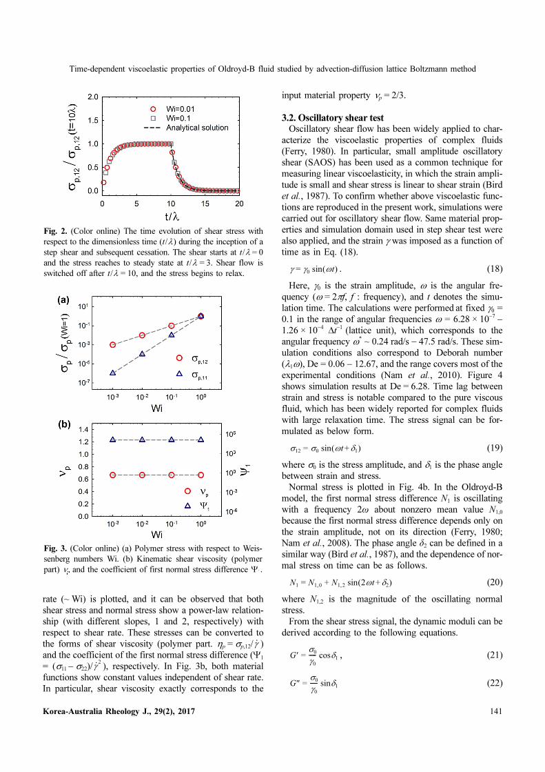
Stress relaxation after cessation of shear flow was also
investigated. At first, shear flow was applied in the same
manner to the previous test. Shearing was stopped after
shear stress reached steady state (t = 10λ), and stress
relaxation was observed (Fig. 2). In this test, the relaxation
behavior was the same for both Wi = 0.01 and Wi = 0.1
when the stress and time are normalized. For Oldroyd-B
fluids, stress relaxation can be predicted by the analytical
solution (Eq. (17)), and the simulation agrees well with
the predictions regardless of Wi.
. (17)
Oldroyd-B fluid (or Boger fluid) does not show any
shear rate dependency in shear viscosity (Boger, 1977),
and this Newtonian behavior is also reflected in our sim-
ulation. In Fig. 3a, the polymer stress with respect to shear
G = 1
λ1
-----– C I–( ) + C ∇u⋅ ∇u( )T+ C⋅
∇ σp⋅
γ·
λ1γ·
σp 12, t( ) = σp 21, t( ) = ηpγ· 1 e
t/λ1
–
–( )
σp 11, t( ) = 2ηpλ1γ·2
1 et/λ
1–
–( ) + 2ηpλ1γ·2
tet/λ
1–
σp 12, t( ) = σp 12, t0( )et t
0–( )/λ
1–
Fig. 1. (Color online) Transient behavior of polymer stress at Wi
= 0.01 and 0.1. (a) Time evolution of σp,12. (b) Time evolution of
σp,11. Black dashed lines are the analytical solutions obtained by
Eqs. (15) and (16). The stress was normalized by the reference
value (analytical solution for Wi = 0.1 at t = 10λ).
Time-dependent viscoelastic properties of Oldroyd-B fluid studied by advection-diffusion lattice Boltzmann method
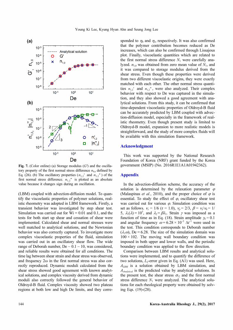
Korea-Australia Rheology J., 29(2), 2017 141
rate (~ Wi) is plotted, and it can be observed that both
shear stress and normal stress show a power-law relation-
ship (with different slopes, 1 and 2, respectively) with
respect to shear rate. These stresses can be converted to
the forms of shear viscosity (polymer part. ηp = σp,12/ )
and the coefficient of the first normal stress difference (Ψ1
= (σ11 − σ22)/ ), respectively. In Fig. 3b, both material
functions show constant values independent of shear rate.
In particular, shear viscosity exactly corresponds to the
input material property νp = 2/3.
3.2. Oscillatory shear testOscillatory shear flow has been widely applied to char-
acterize the viscoelastic properties of complex fluids
(Ferry, 1980). In particular, small amplitude oscillatory
shear (SAOS) has been used as a common technique for
measuring linear viscoelasticity, in which the strain ampli-
tude is small and shear stress is linear to shear strain (Bird
et al., 1987). To confirm whether above viscoelastic func-
tions are reproduced in the present work, simulations were
carried out for oscillatory shear flow. Same material prop-
erties and simulation domain used in step shear test were
also applied, and the strain γ was imposed as a function of
time as in Eq. (18).
. (18)
Here, γ0 is the strain amplitude, ω is the angular fre-
quency (ω = 2πf, f : frequency), and t denotes the simu-
lation time. The calculations were performed at fixed γ0 =
0.1 in the range of angular frequencies ω = 6.28 × 10⁻⁷−
1.26 × 10⁻⁴ Δt−1 (lattice unit), which corresponds to the
angular frequency ω* ~ 0.24 rad/s − 47.5 rad/s. These sim-
ulation conditions also correspond to Deborah number
(λ1ω), De = 0.06 − 12.67, and the range covers most of the
experimental conditions (Nam et al., 2010). Figure 4
shows simulation results at De = 6.28. Time lag between
strain and stress is notable compared to the pure viscous
fluid, which has been widely reported for complex fluids
with large relaxation time. The stress signal can be for-
mulated as below form.
(19)
where σ0 is the stress amplitude, and δ1 is the phase angle
between strain and stress.
Normal stress is plotted in Fig. 4b. In the Oldroyd-B
model, the first normal stress difference N1 is oscillating
with a frequency 2ω about nonzero mean value N1,0
because the first normal stress difference depends only on
the strain amplitude, not on its direction (Ferry, 1980;
Nam et al., 2008). The phase angle δ2 can be defined in a
similar way (Bird et al., 1987), and the dependence of nor-
mal stress on time can be as follows.
(20)
where N1,2 is the magnitude of the oscillating normal
stress.
From the shear stress signal, the dynamic moduli can be
derived according to the following equations.
, (21)
(22)
γ·
γ·2
γ = γ0 sin ωt( )
σ12 = σ0 sin ωt δ1+( )
N1 = N1 0, + N1 2, sin 2ωt δ2+( )
G′ = σ0
γ0
----- cosδ1
G″ = σ0
γ0
----- sinδ1
Fig. 3. (Color online) (a) Polymer stress with respect to Weis-
senberg numbers Wi. (b) Kinematic shear viscosity (polymer
part) νp and the coefficient of first normal stress difference Ψ1.
Fig. 2. (Color online) The time evolution of shear stress with
respect to the dimensionless time (t/λ) during the inception of a
step shear and subsequent cessation. The shear starts at t/λ = 0
and the stress reaches to steady state at t/λ = 3. Shear flow is
switched off after t/λ = 10, and the stress begins to relax.

Young Ki Lee, Kyung Hyun Ahn and Seung Jong Lee
142 Korea-Australia Rheology J., 29(2), 2017
where G' and G'' are the storage modulus and the loss
modulus.
In Fig. 5a, the dynamic moduli are plotted as a function
of Deborah number (De). At low Deborah number (De <
1), both storage modulus and loss modulus increase with
slopes 2 and 1, respectively, and they coincide at De ~ 1.
At higher Deborah number (De > 1), the storage modulus
shows a plateau, while the loss modulus keeps on increas-
ing with De. This means that the solvent contribution
becomes more dominant for De > 1. In small strain ampli-
tude region, the dynamic moduli of Oldroyd-B fluids can
be derived as follows, and our simulation corresponds
well with the analytical solution.
, (23)
. (24)
The complex viscosity can also be obtained as in Eq.
(25).
. (25)
As shown in Fig. 5b, the complex viscosity shows two
plateau regions. At low De limit (De < 0.1), the complex
viscosity shows the first plateau, which corresponds to η0.
With the increase in De, it shows shear thinning behavior,
and eventually reaches a secondary plateau (De ~ 10),
which corresponds to ηs. This result means that the poly-
mer contribution becomes relatively weak as De increases,
and it corresponds to the well-known rheological charac-
teristics of Boger fluids (Nam et al., 2010).
A popular way to show the response of a viscoelastic
fluid upon the oscillatory shear is to plot a closed loop of
stress versus strain or stress versus rate of strain, namely
Lissajous plot. In the Lissajous plot, an elliptical curve is
observed in the linear viscoelastic regime, while non-ellip-
tical shape is observed in the nonlinear viscoelastic regime
G′ ω( ) = η0ωλ1 λ2–( )ω
1 λ1
2ω
2+
-----------------------
G″ ω( ) = η0ω1 λ+ 1λ2ω
2
1 λ1
2ω
2+
------------------------
η*ω( ) =
G′2 ω( ) G″2ω( )+
ω-------------------------------------------
Fig. 5. (Color online) (a) Dynamic moduli and (b) complex vis-
cosity obtained by LBM simulation (symbols) and theoretical
prediction (lines). They are plotted as a function of Deborah
number (λ1ω). The parameter sets are η0 = 5/6, β = 1/5, λ1= 105,
and λ2 = βλ1. Cross-over point of dynamic moduli corresponds to
De = 1, and the plateau modulus (GN) is observed at high De. η0
and ηs correspond to the complex viscosity at low De limit and
at high De limit, respectively.
Fig. 4. (Color online) (a) Sinusoidal input shear strain of ampli-
tude γ0 = 0.1 at angular frequency ω = 6.28 × 10⁻⁵ Δt−1
(De = 6.28) produces sinusoidal total shear stress. The total
shear stress (black solid line) is plotted together with polymer
stress (red dot). Time lag between stress and strain is clearly
observed, which is defined as the phase angle δ1. (b) The first
normal stress difference oscillates with an angular frequency 2ω
with a nonzero mean value (N1,0).

Time-dependent viscoelastic properties of Oldroyd-B fluid studied by advection-diffusion lattice Boltzmann method
Korea-Australia Rheology J., 29(2), 2017 143
(Hyun et al., 2011). This trend in the Lissajous curve is
well reproduced through our simulation. In Fig. 6, stress
(shear and normal stress difference) versus strain is plot-
ted. At low De (De = 0.06), both total shear stress σ12 and
polymer shear stress σp,12 maintain ellipsoidal shape, but
the curves change to non-elliptical shape as De increases.
The area inside of the Lissajous plot provides information
on the relative contribution of polymer phase in the fluid.
The smaller area is observed for polymer stress than total
shear stress, and the more reduced area is clearly observed
as De increases. This can be interpreted as a reduced con-
tribution of polymers at large strain amplitude, which also
corresponds to the trend of the complex viscosity in Fig.
5b. Contrast to the shear stress σ12, the first normal stress
difference N1 does not show elliptic curve at all, and their
phase angle δ2 also shows quite different behavior from δ1.
In our simulation, δ2 decreases with De, and it shows
minus (−) values after De ~ 1. On the other hand, δ1 is
always positive. In addition, N1 vs strain curve changes its
shape after De ~ 1 (convex to concave), which corresponds
to experiments with Boger fluid (Nam et al., 2010).
In the small amplitude oscillatory shear (SAOS) limit,
the first normal stress difference N1 can be reformulated as
follows. n1,0 can be defined in terms of zero mean value of
N1 (N1,0) and strain amplitude γ0, which corresponds to the
storage modulus G' of Oldroyd-B fluid (Bird et al., 1987;
Ferry, 1980).
. (26)
The other quantities ( and ) can also be related
to the normal stress difference, and they are co-related
with phase angle (Nam et al., 2008;
Nam et al., 2010).
, (27)
. (28)
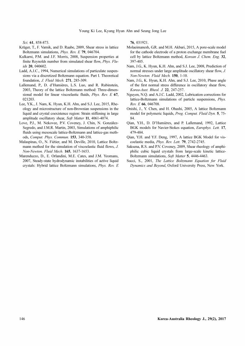
The characteristics of and are clearly reflected
in our simulation. In Fig. 7a, G' obtained from shear stress
and n1,0 derived from normal stress are plotted together.
Even though they are obtained from different material
functions, both results are well coincided with each other,
and moreover, they correspond well with analytical solu-
tions.
Finally, the quantities and are plotted in Fig.
7b. With respect to De, the slope of is 3 at low De,
while it becomes −1 at high De. The slope of shows
a sudden decrease after increasing with the slope of 2. At
higher De, a sudden increase is captured with an increase
of De, and eventually, it reaches a plateau. These obser-
vations not only follow theoretical predictions (Eqs. (27)
and (28)), but also coincide to the reported rheological
behavior of Boger fluids (Nam et al., 2010).
4. Conclusions
Time-dependent viscoelastic properties of Oldroyd-B
fluids were investigated by the lattice Boltzmann method
n1 0, = N1,0/γ 0
2 = G′ ω( )
n1 2, ′ n1 2, ″
δ2 = tan1–
n1 2, ′/n1 2, ″( )
n1,2′ = N1 2, cosδ2/γ 0
2 = G″ ω( )−
1
2---G″ 2ω( )
n1,2″ = N1 2, cosδ2/γ 0
2 = G– ′ ω( )+
1
2---G′ 2ω( )
n1,2′ n1,2″
n1,2′ n1,2″n1,2′
n1,2″
Fig. 6. (Color online) Lissajous plots: stress versus strain. The shear stress and the first normal stress difference are represented for
various Deborah numbers (De = λ1ω), and the curves are normalized by their amplitudes. The simulation parameters are η0 = 1/6, β
= 1/5, λ1 = 105, and λ2 = βλ1.
Young Ki Lee, Kyung Hyun Ahn and Seung Jong Lee
144 Korea-Australia Rheology J., 29(2), 2017
(LBM) coupled with advection-diffusion model. To quan-
tify the viscoelastic properties of polymer solutions, real-
istic rheometry was adopted in LBM framework. Firstly, a
transient behavior was investigated by step shear test.
Simulation was carried out for Wi = 0.01 and 0.1, and the
tests for both start up shear and cessation of shear were
implemented. Calculated shear and normal stresses were
well matched to analytical solutions, and the Newtonian
behavior was also correctly captured. To investigate more
complex viscoelastic properties of the fluid, simulation
was carried out in an oscillatory shear flow. The wide
range of Deborah number, De ~ 0.1 − 10, was considered,
and reliable results were obtained for all conditions. The
time lag between shear strain and shear stress was observed,
and frequency 2ω in the first normal stress was also cor-
rectly reproduced. Dynamic moduli calculated from the
shear stress showed good agreement with known analyt-
ical solutions, and complex viscosity derived from dynamic
moduli also correctly followed the general behavior of
Oldroyd-B fluid. Complex viscosity showed two plateau
regions at both low and high De limits, and they corre-
sponded to η0 and ηs, respectively. It was also confirmed
that the polymer contribution becomes reduced as De
increases, which can also be confirmed through Lissajous
plot. Finally, viscoelastic quantities which are related to
the first normal stress difference N1 were carefully ana-
lyzed. n1,0 was obtained from zero mean value of N1, and
it was compared to storage modulus derived from the
shear stress. Even though these properties were derived
from two different viscoelastic origins, they were exactly
matched with each other. The other normal stress quanti-
ties and , were also analyzed. Their complex
behavior with respect to De was captured in the simula-
tion, and they also showed a good agreement with ana-
lytical solutions. From this study, it can be confirmed that
time-dependent viscoelastic properties of Oldroyd-B fluid
can be accurately predicted by LBM coupled with advec-
tion-diffusion model, especially in the framework of real-
istic rheometry. Even though present study is limited to
Oldroyd-B model, expansion to more realistic models is
straightforward, and the study of more complex fluids will
be available with this simulation framework.
Acknowledgment
This work was supported by the National Research
Foundation of Korea (NRF) grant funded by the Korea
government (MSIP) (No. 2016R1E1A1A01942362).
Appendix
In the advection-diffusion scheme, the accuracy of the
solution is determined by the relaxation parameter ϕ
(Malaspinas et al., 2010), and the proper choice of ϕ is
essential. To study the effect of ϕ, oscillatory shear test
was carried out for various ϕ. Simulation condition was
set as follows. νs = 1/6 (τ = 1.0), νp = 2/3, β = νs/ν0 = 1/
5, λ1(λ) = 105, and λ2 = βλ1. Strain γ was imposed as a
function of time as in Eq. (18). Strain amplitude γ0 = 0.1
and angular frequency ω = 6.28 × 10⁻⁵ Δt−1 were used in
the test. This condition corresponds to Deborah number
(λ1ω), De = 6.28. The size of the simulation domain was
100 × 102. The moving wall boundary condition was
imposed in both upper and lower walls, and the periodic
boundary condition was applied to the flow direction.
Comparison between LBM results and analytical solu-
tions were implemented, and to quantify the difference of
two solutions, L2-error given in Eq. (A1) was used. Here,
ALBM is a solution obtained by LBM simulation, and
AAnalytical is the predicted value by analytical solutions. In
the present test, the shear stress σ12 and the first normal
stress difference N1 were analyzed. The analytical solu-
tions for each rheological property were obtained by solv-
ing Eqs. (19)-(28).
n1,2′ n1,2″
Fig. 7. (Color online) (a) Storage modulus (G') and the oscilla-
tory property of the first normal stress difference n1,0 defined by
Eq. (26). (b) The oscillatory properties ( and ) of the
first normal stress difference. is plotted as an absolute
value because it changes sign during an oscillation.
n1 2, ′ n1 2, ″n1 2, ″

Time-dependent viscoelastic properties of Oldroyd-B fluid studied by advection-diffusion lattice Boltzmann method
Korea-Australia Rheology J., 29(2), 2017 145
. (A1)
In the test, L2-error was measured in the time range ωt
= 0~π/4, and it was discretized as the total number of bins
N = 250 in the analysis.
In Fig. A1, time evolution of the stress signal is plotted
for various ϕ (ϕ = 0.9, ϕ = 0.6, and ϕ = 0.51). At ϕ = 0.9,
inaccurate solutions are clearly captured in both σ12 and
N1. Discrepancies between LBM simulation and analytical
solutions are observed not only in the maximum peak but
also in phase angle, and with a decrease of ϕ, more accu-
rate solutions are obtained. To quantify solution depen-
dency for the parameter ϕ, L2-errors of σ12 and N1 are
analyzed (Fig. A2). In case of shear stress, at ϕ = 0.9,
error (σ12) = 9.45 × 10⁻²; at ϕ = 0.6, error (σ12) = 5.38 ×
10−2; at ϕ = 0.51, error (σ12) = 1.14 × 10⁻². In case of the
first normal stress difference, at ϕ = 0.9, error (N1) = 2.78
× 10−1; at ϕ = 0.6, error (N1) = 1.12 × 10⁻¹; at ϕ = 0.51,
error (N1) = 1.46 × 10⁻². In the test limit, large error was
captured in N1 than σ12 (about 200%), and the error dif-
ference between two properties becomes reduced with the
decrease in ϕ (from 300% at ϕ = 0.9 to 130% at ϕ = 0.51).
In both cases, a more accurate solution was obtained as ϕ
decreased, and finally the most accurate solution was con-
firmed at ϕ = 0.51.
References
Aidun, C.K. and J.R. Clausen, 2010, Lattice-Boltzmann method
for complex flows, Annu. Rev. Fluid Mech. 42, 439-472.
Bird, R.B., C.F. Curtiss, R.C. Armstrong, and O. Hassager, 1987,
Dynamics of Polymeric Liquids, Vol.2: Kinetic Theory, 2nd
ed.,
Wiley, New York.
Boger, D.V., 1977, A highly elastic constant-viscosity fluid, J.
Non-Newton. Fluid Mech. 3, 87-91.
Denniston, C., E. Orlandini, and J.M. Yeomans, 2001, Lattice
Boltzmann simulations of liquid crystal hydrodynamics, Phys.
Rev. E 63, 056702.
Ferry, J.D., 1980, Viscoelastic Properties of Polymers, 3rd ed.,
Wiley, New York.
Ginzburg, I., G. Silva, and L. Talon, 2015, Analysis and improve-
ment of Brinkman lattice Boltzmann schemes: Bulk, boundary,
interface. Similarity and distinctness with finite elements in
heterogeneous porous media, Phys. Rev. E 91, 023307.
Giraud, L., D. d’Humières, and P. Lallemand, 1998, A lattice
Boltzmann model for Jeffreys viscoelastic fluid, Europhys.
Lett. 42, 625-630.
Gross, M., T. Krüger, and F. Varnik, 2014, Rheology of dense
suspensions of elastic capsules: Normal stresses, yield stress,
jamming and confinement effects, Soft Matter 10, 4360-4372.
Guo, Z., C. Zheng, and B. Shi, 2002, Discrete lattice effects on
the forcing term in the lattice Boltzmann method, Phys. Rev. E
65, 046308.
He, X. and L.S. Luo, 1997, Lattice Boltzmann model for the
incompressible Navier-Stokes equation, J. Stat. Phys. 88, 927-
944.
Hyun, K., M. Wilhelm, C.O. Klein, K.S. Cho, J.G. Nam, K.H.
Ahn, S.J. Lee, R.H. Ewoldt, and G.H. McKinley, 2011, A
review of nonlinear oscillatory shear tests: Analysis and appli-
cation of large amplitude oscillatory shear (LAOS), Prog.
Polym. Sci. 36, 1697-1753.
Ispolatov, I. and M. Grant, 2002, Lattice Boltzmann method for
viscoelastic fluids, Phys. Rev. E 65, 056704.
James, D.F., 2009, Boger fluids, Annu. Rev. Fluid Mech. 41, 129-
142.
Kromkamp, J., D. van den Ende, D. Kandhai, R. van der Sman,
and R. Boom, 2006, Lattice Boltzmann simulation of 2D and
3D non-Brownian suspensions in Couette flow, Chem. Eng.
error A( ) = 1
N----
i 1=
N
∑Ai LBM, Ai Analytical,–
Ai Analytical,
-----------------------------------------2
Fig. A2. (Color online) The L2-error for the stresses with respect
to ϕ. (a) Result for σ12. (b) Result for N1.
Fig. A1. (Color online) Time evolution of stress signal (De =
6.25). (a) Simulation results for shear stress σ12. (b) Simulation
results for the first normal stress difference N1. Red circle and
blue square denote analytical solutions of σ12 and N1, respec-
tively. Here, each property was normalized by reference value
σ12,ref (the maximum value of σ12 obtained by analytical solution).
Young Ki Lee, Kyung Hyun Ahn and Seung Jong Lee
146 Korea-Australia Rheology J., 29(2), 2017
Sci. 61, 858-873.
Krüger, T., F. Varnik, and D. Raabe, 2009, Shear stress in lattice
Boltzmann simulations, Phys. Rev. E 79, 046704.
Kulkarni, P.M. and J.F. Morris, 2008, Suspension properties at
finite Reynolds number from simulated shear flow, Phys. Flu-
ids 20, 040602.
Ladd, A.J.C., 1994, Numerical simulations of particulate suspen-
sions via a discretized Boltzmann equation. Part I. Theoretical
foundation, J. Fluid Mech. 271, 285-309.
Lallemand, P., D. d’Humières, L.S. Luo, and R. Rubinstein,
2003, Theory of the lattice Boltzmann method: Three-dimen-
sional model for linear viscoelastic fluids, Phys. Rev. E 67,
021203.
Lee, Y.K., J. Nam, K. Hyun, K.H. Ahn, and S.J. Lee, 2015, Rhe-
ology and microstructure of non-Brownian suspensions in the
liquid and crystal coexistence region: Strain stiffening in large
amplitude oscillatory shear, Soft Matter 11, 4061-4074.
Love, P.J., M. Nekovee, P.V. Coveney, J. Chin, N. González-
Segredo, and J.M.R. Martin, 2003, Simulations of amphiphilic
fluids using mesoscale lattice-Boltzmann and lattice-gas meth-
ods, Comput. Phys. Commun. 153, 340-358.
Malaspinas, O., N. Fiétier, and M. Deville, 2010, Lattice Boltz-
mann method for the simulation of viscoelastic fluid flows, J.
Non-Newton. Fluid Mech. 165, 1637-1653.
Marenduzzo, D., E. Orlandini, M.E. Cates, and J.M. Yeomans,
2007, Steady-state hydrodynamic instabilities of active liquid
crystals: Hybrid lattice Boltzmann simulations, Phys. Rev. E
76, 031921.
Molaeimanesh, G.R. and M.H. Akbari, 2015, A pore-scale model
for the cathode electrode of a proton exchange membrane fuel
cell by lattice Boltzmann method, Korean J. Chem. Eng. 32,
397-405.
Nam, J.G., K. Hyun, K.H. Ahn, and S.J. Lee, 2008, Prediction of
normal stresses under large amplitude oscillatory shear flow, J.
Non-Newton. Fluid Mech. 150, 1-10.
Nam, J.G., K. Hyun, K.H. Ahn, and S.J. Lee, 2010, Phase angle
of the first normal stress difference in oscillatory shear flow,
Korea-Aust. Rheol. J. 22, 247-257.
Nguyen, N.Q. and A.J.C. Ladd, 2002, Lubrication corrections for
lattice-Boltzmann simulations of particle suspensions, Phys.
Rev. E 66, 046708.
Onishi, J., Y. Chen, and H. Ohashi, 2005, A lattice Boltzmann
model for polymeric liquids, Prog. Comput. Fluid Dyn. 5, 75-
84.
Qian, Y.H., D. D’Humières, and P. Lallemand, 1992, Lattice
BGK models for Navier-Stokes equation, Europhys. Lett. 17,
479-484.
Qian, Y.H. and Y.F. Deng, 1997, A lattice BGK Model for vis-
coelastic media, Phys. Rev. Lett. 79, 2742-2745.
Saksena, R.S. and P.V. Coveney, 2009, Shear rheology of amphi-
philic cubic liquid crystals from large-scale kinetic lattice-
Boltzmann simulations, Soft Matter 5, 4446-4463.
Succi, S., 2001, The Lattice Boltzmann Equation for Fluid
Dynamics and Beyond, Oxford University Press, New York.