UNIVERSITI PUTRA MALAYSIA

TIME DOMAIN REFLECTOMETRY COMPUTATIONAL TECHNIQUE USING AGILENT VEE

NUR SHARIZAN MOHAMED DAN

IPM 2007 4

TIME DOMAIN REFLECTOMETRY COMPUTATIONAL TECHNIQUE

USING AGILENT VEE

By

NUR SHARIZAN MOHAMED DAN

Thesis Submitted to the School of Graduate Studies, Universiti Putra Malaysia, in Fulfilment of the Requirements for the Degree of Master of Science

October 2007

To My Family, Friends and The Beloved.

ii

Abstract of thesis presented to the Senate of Universiti Putra Malaysia in fulfilment of the requirement for the degree of Master of Science

TIME DOMAIN REFLECTOMETRY COMPUTATIONAL TECHNIQUE USING AGILENT VEE

By

NUR SHARIZAN MOHAMED DAN

October 2007

Chairman : Zulkifly Abbas, PhD Institute : Institute of Mathematical Research This thesis describes the time domain reflectometry computational technique to locate

discontinuities in transmission line using Agilent VEE version 6. The reflection

coefficient measurement data were transformed from frequency domain into time

domain using Fast Fourier Transform (FFT) technique. Measurements were done on

waveguides and coaxial cable using HP 8720B network analyzer. The vector network

analyzer (VNA) has a time domain capability where transformation from frequency to

time domain data is realized using chirp z-transform (CZT) which can be utilized to

locate short circuit discontinuities. Unfortunately, the VNA is heavy, bulky and an

expensive way of simulating time domain reflectometry measurement. The frequency-

to-time measurement option is not a readily built in feature but needs to be purchased

before it is included in the VNA in which it comes at a higher cost for end user.

Additionally, frequency-to-time measurement option of the VNA has limited capability

iii

with only selected transformation algorithm, window and gating method. This motivates

the transformation using computer software instead of VNA to transform data, thus, the

development of transformation software.

All the measurements and calculations were implemented using transformation software

developed using Agilent VEE version 6. The analysis on resolution was done and

parameters that affects the resolution; number of points and frequency range, was

analyzed. The transformation software transforms frequency domain data to time

domain. The peaks in the measurement data represent discontinuity in the test

components/devices. Measurements were done on combinations of well define

components which includes WR-90 waveguides and RG402 coaxial cable. The

performance of the transformation software was tested by comparing the results with

true physical measurement of the devices. The results show that the reflection coefficient

obtained from the software is in good agreement with the VNA in terms of the location

of discontinuity with both VNA and transformation software having ≈5% deviation with

the true physical value. The transformation software results are as reliable as the VNA.

This transformation software is flexible, cheap and easy to use. It is ready to be

incorporated into mobile computer and can be used with any frequency domain

measurement device.

iv

Abstrak tesis yang dikemukakan kepada Senat Universiti Putra Malaysia sebagai memenuhi keperluan untuk ijazah Master Sains

TEKNIK PENGIRAAN PANTULAN DOMAIN MASA MENGGUNAKAN AGILENT VEE

Oleh

NUR SHARIZAN MOHAMED DAN

Oktober 2007

Pengerusi : Zulkifly Abbas, PhD Institute : Institute Penyelidikan Matematik Tesis ini memperihalkan tentang teknik pengiraan pantulan domain masa untuk

menentukan ketidakselanjaran dalam garis pancaran menggunakan Agilent VEE versi 6.

Data ukuran pekali pantulan ditukar bentuk dari domain frekuensi ke domain masa

dengan menggunakan teknik Jelmaan Fourier Cepat (FFT). Pengukuran dilakukan ke

atas pandugelombang dan kabel sepaksi menggunakan Penganalisis Rangkaian Vektor

(VNA) HP 8720B. VNA mempunyai kebolehan pengukuran dalam domain masa untuk

menentukan ketidakselanjaran dimana penukaran data dari bentuk domain frekuensi ke

domain masa dilakukan dengan menggunakan algoritma Jelmaan Z Chirp (CZT).

Walaubagaimanapun, VNA adalah mesin yang berat, besar dan merupakan cara yang

mahal untuk mensimulasikan pengukuran teknik pantulan domain masa. Pilihan

pengukuran domain frekuensi ke domain masa merupakan satu pilihan yang perlu dibeli

sebelum ia disertakan bersama VNA dengan harga yang lebih mahal. Di samping itu,

v

pilihan ukuran domain frekuensi ke domain masa VNA adalah terhad dengan hanya

mempunyai transformasi terpilih dan cara tetingkap dan pepintu tertentu sahaja. Ini

memberi ilham untuk menggunakan perisian komputer untuk melakukan transformasi

bagi menggantikan transformasi data menggunakan VNA.

Kesemua ukuran dan kiraan telah dilakukan dengan menggunakan perisian transformasi

yang diprogram menggunakan Agilent VEE 6. Analisis resolusi telah dijalankan dan

parameter yang boleh mempengaruhi resolusi; bilangan titik dan julat frekuensi, telah

dikaji. Perisian transformasi berjaya menukarkan data domain frekuensi ke domain

masa. Puncak dalam data pengukuran mewakili ketidakselanjaran dalam komponen/alat

yang diuji. Ukuran telah dijalankan ke atas kombinasi komponen yang diketahui ciri-

cirinya termasuk pandugelombang siri WR-90 dan kabel sepaksi siri RG402. Prestasi

perisian transformasi telah diuji melalui perbandingan keputusan dengan ukuran fizikal

sebenar komponen. Keputusan menunjukan pekali pantulan yang diperolehi dari perisian

transformasi dan VNA adalah dari segi penentuan ketidakselanjaran adalah memuaskan

dan kedua-dua keputusan VNA dan perisian transformasi mempunyai pembezaan

sebanyak ≈ 5 % dengan nilai fizikal sebenar. Keputusan perisian transformasi adalah

setanding VNA. Perisian transformasi ini boleh diubah, murah dan mudah untuk

digunakan. Ia juga sedia digunakan bersama komputer mudah alih atau sebarang alat

ukuran domain frekuensi.

vi

ACKNOWLEDGEMENTS

Alhamdulillah, many thanks and praises be with God Almighty for all the blessings

rained upon this life.

My greatest thanks to Dr. Zulkifly Abbas whose kind enough to provide supervision

until the completion of this thesis. Thank you for your supervision, guidance and words

of wisdom.

To my parents, Mohamed Dan b. Jantan and Amelia Yow bt. Abdullah, whom I cannot

live without; it’s never too old to learn something new. My deepest gratitude for

everything.

My warm wishes and thanks to the members of Electromagnetic Lab and friends in

UPM, thank you for your help and support. This journey would’ve been down the

boredom road if it wasn’t for you guys.

Lastly, to the beloved; you gave me courage, you brought me happiness, you brought

sorrows I never imagine I could feel but you also pour me your love and brighten the

night skies with your stars. Even if we could never be together, you are always in a

special place deep inside this wretched heart. A thousand thank you won’t do justice, but

it’s the only thing I could offer; thank you.

vii

viii

This thesis was submitted to the Senate of Universiti Putra Malaysia and has been accepted as fulfilment of the requirement for the degree of Master of Science. The members of the Supervisory Committee were as follows: Zulkifly Abbas, PhD Lecturer Institute of Mathematical Research Universiti Putra Malaysia. (Chairman) Kaida Khalid, PhD Professor Faculty of Science Universiti Putra Malaysia. (Member)

________________________________

AINI IDERIS, PhD Professor and Dean School of Graduate Studies Universiti Putra Malaysia Date: 22 January 2008

ix

DECLARATION

I hereby declare that the thesis is based on my original work except for quotations and citations which have been duly acknowledged. I also declare that it has not been previously or concurrently submitted for any other degree at UPM or other institutions.

________________________________

NUR SHARIZAN MOHAMED DAN

Date: 6 November 2007

x

TABLE OF CONTENTS Page DEDICATION ii ABSTRACT iii ABSTRAK v ACKNOWLEDGEMENTS vii APPROVAL viii DECLARATION x LIST OF TABLES xiii LIST OF FIGURES xiv LIST OF ABBREVIATIONS xix CHAPTER 1 INTRODUCTION 1 - 1

1.1 An Overview of the Determination of Material Discontinuities 1 - 2 1.1.1 Technology and Application in Determination of

Material Discontinuities 1 - 3 1.1.2 Vector Network Analyzer 1 - 5

1.2 Problem Statement 1 - 6 1.3 Objectives 1 - 7

1.4 The Scope of Thesis 1 - 8 2 LITERATURE REVIEW 2 - 1 2.1 Introduction to the Time Domain Reflectometry ` 2 - 2

2.1.1 The Time Domain Reflectometry 2 - 6 2.1.2 Time Domain Measurement using Vector Network

Analyzer 2 - 8 2.2 Frequency-to-Time Domain Transformation 2 - 9

2.2.1 Review of Frequency-to-Time Domain Transformation 2 - 10 3 THEORY OF TIME DOMAIN TRANSFORMATION

TECHNIQUE 3 - 1 3.1 Principle of Time Domain Reflectometry Technique 3 - 2 3.1.1 Propagation on Transmission Line 3 - 3 3.1.2 Locating Mismatches and Analyzing Reflections 3 - 6 3.1.3 Discontinuities on the Line 3 - 10 3.1.4 Multiple Discontinuities 3 - 12 3.2 The Vector Network Analyzer 3 - 14 3.2.1 The HP 9720B VNA Measurement 3 - 14

xi

3.2.2 Vector Network Analyzer Frequency-to-Time Domain Measurement 3 - 15

3.3 Theory of Frequency-to-Time Domain Transformation 3 - 24 3.3.1 Fast Fourier Transform (FFT) 3 - 24

3.4 FFT in MATLAB 3 - 30 4 METHODOLOGY 4 - 1

4.1 Frequency-to-Time Domain Software Development 4 - 2 4.1.1 Software Development Using Agilent VEE 4 - 4 4.1.2 MATLAB® Scripts in Transformation Software 4 - 17

4.2 Measurement Setup for Reflection Measurement 4 - 21 4.3 Setup for Performance Testing of Frequency-to-Time

Transformation Software 4 - 22 5 ANALYSIS OF TRANSFORMATION OF FREQUENCY

DOMAIN DATA TO TIME DOMAIN 5 - 1 5.1 Frequency-to-Time Domain Transformation 5 - 1 5.2 Effect of Transformation Parameters 5 - 2 5.2.1 Resolution Analysis 5 - 4

5.2.2 Magnitude Analysis 5 - 33 5.3 Analysis of Frequency-to-Time Domain Transformation

Software 5 - 41 5.3.1 Analysis on Number of Points 5 - 42 5.3.2 Analysis on Frequency Range 5 - 51

5.4 Performance Testing of Frequency-to-Time Transformation Software 5 - 59

6 CONCLUSION AND SUGGESTION 6 - 1 6.1 Conclusion 6 - 1 6.2 Main Contributions 6 - 2 6.3 Recommendations for Further Work 6 - 3 6.3.1 Software Feature Enhancement 6 - 3

6.3.2 Software Incorporated Into a Standalone System 6 - 4 6.3.3 Other Applications 6 - 4

REFERENCES R - 1 APPENDICES A - 1 BIODATA OF THE AUTHOR V - 1

xii

LIST OF TABLES

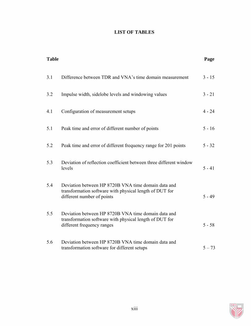
Table Page 3.1 Difference between TDR and VNA’s time domain measurement 3 - 15

3.2 Impulse width, sidelobe levels and windowing values 3 - 21

4.1 Configuration of measurement setups 4 - 24

5.1 Peak time and error of different number of points 5 - 16

5.2 Peak time and error of different frequency range for 201 points 5 - 32

5.3 Deviation of reflection coefficient between three different window levels 5 - 41

5.4 Deviation between HP 8720B VNA time domain data and transformation software with physical length of DUT for different number of points 5 - 49

5.5 Deviation between HP 8720B VNA time domain data and transformation software with physical length of DUT for different frequency ranges 5 - 58

5.6 Deviation between HP 8720B VNA time domain data and transformation software for different setups 5 – 73

xiii

LIST OF FIGURES

Figure Page 1.1 The HP 8720B VNA 1 - 6

2.1 Simplified block diagram of a basic FDR setup 2 - 4

2.2 Simplified block diagram of a generalized VNA setup 2 - 5

2.3 Simplified block diagram of a basic TDR setup 2 - 6

3.1 Voltage vs time at a particular point on a mismatched transmission line driven with a step of height Ei 3 - 3

3.2 The classical model for a transmission line 3 - 3

3.3 TDR displays for typical loads (a) Open circuit termination )( ∞=LZ 3 - 7

(b) Short circuit termination )0( =LZ 3 - 7 (c) Line terminated in oL ZZ 2= 3 - 8

(d) Line terminated in oL ZZ21

= 3 - 8

3.4 Oscilloscope displays for various complex ZL 3 - 9

3.5 Intermediate positions along a transmission line 3 - 11

3.6 Equivalent representation 3 - 11

3.7 Special case of series R-L circuit 3 - 11

xiv

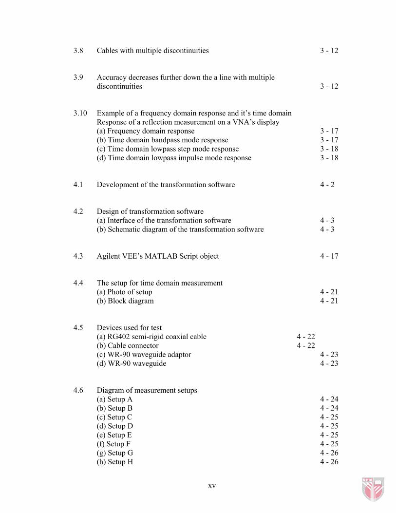
3.8 Cables with multiple discontinuities 3 - 12

3.9 Accuracy decreases further down the a line with multiple discontinuities 3 - 12

3.10 Example of a frequency domain response and it’s time domain Response of a reflection measurement on a VNA’s display (a) Frequency domain response 3 - 17 (b) Time domain bandpass mode response 3 - 17

(c) Time domain lowpass step mode response 3 - 18 (d) Time domain lowpass impulse mode response 3 - 18

4.1 Development of the transformation software 4 - 2

4.2 Design of transformation software (a) Interface of the transformation software 4 - 3 (b) Schematic diagram of the transformation software 4 - 3

4.3 Agilent VEE’s MATLAB Script object 4 - 17

4.4 The setup for time domain measurement (a) Photo of setup 4 - 21

(b) Block diagram 4 - 21

4.5 Devices used for test (a) RG402 semi-rigid coaxial cable 4 - 22 (b) Cable connector 4 - 22 (c) WR-90 waveguide adaptor 4 - 23

(d) WR-90 waveguide 4 - 23

4.6 Diagram of measurement setups (a) Setup A 4 - 24

(b) Setup B 4 - 24 (c) Setup C 4 - 25 (d) Setup D 4 - 25 (e) Setup E 4 - 25 (f) Setup F 4 - 25 (g) Setup G 4 - 26 (h) Setup H 4 - 26

xv

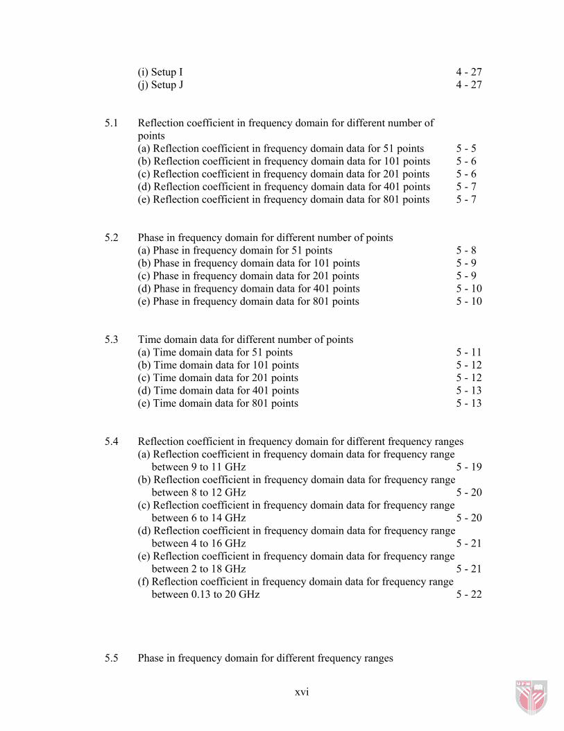
(i) Setup I 4 - 27 (j) Setup J 4 - 27

5.1 Reflection coefficient in frequency domain for different number of points

(a) Reflection coefficient in frequency domain data for 51 points 5 - 5 (b) Reflection coefficient in frequency domain data for 101 points 5 - 6

(c) Reflection coefficient in frequency domain data for 201 points 5 - 6 (d) Reflection coefficient in frequency domain data for 401 points 5 - 7 (e) Reflection coefficient in frequency domain data for 801 points 5 - 7

5.2 Phase in frequency domain for different number of points (a) Phase in frequency domain for 51 points 5 - 8 (b) Phase in frequency domain data for 101 points 5 - 9 (c) Phase in frequency domain data for 201 points 5 - 9 (d) Phase in frequency domain data for 401 points 5 - 10 (e) Phase in frequency domain data for 801 points 5 - 10

5.3 Time domain data for different number of points (a) Time domain data for 51 points 5 - 11 (b) Time domain data for 101 points 5 - 12 (c) Time domain data for 201 points 5 - 12 (d) Time domain data for 401 points 5 - 13 (e) Time domain data for 801 points 5 - 13

5.4 Reflection coefficient in frequency domain for different frequency ranges (a) Reflection coefficient in frequency domain data for frequency range between 9 to 11 GHz 5 - 19 (b) Reflection coefficient in frequency domain data for frequency range between 8 to 12 GHz 5 - 20 (c) Reflection coefficient in frequency domain data for frequency range between 6 to 14 GHz 5 - 20 (d) Reflection coefficient in frequency domain data for frequency range between 4 to 16 GHz 5 - 21 (e) Reflection coefficient in frequency domain data for frequency range between 2 to 18 GHz 5 - 21 (f) Reflection coefficient in frequency domain data for frequency range between 0.13 to 20 GHz 5 - 22

5.5 Phase in frequency domain for different frequency ranges

xvi

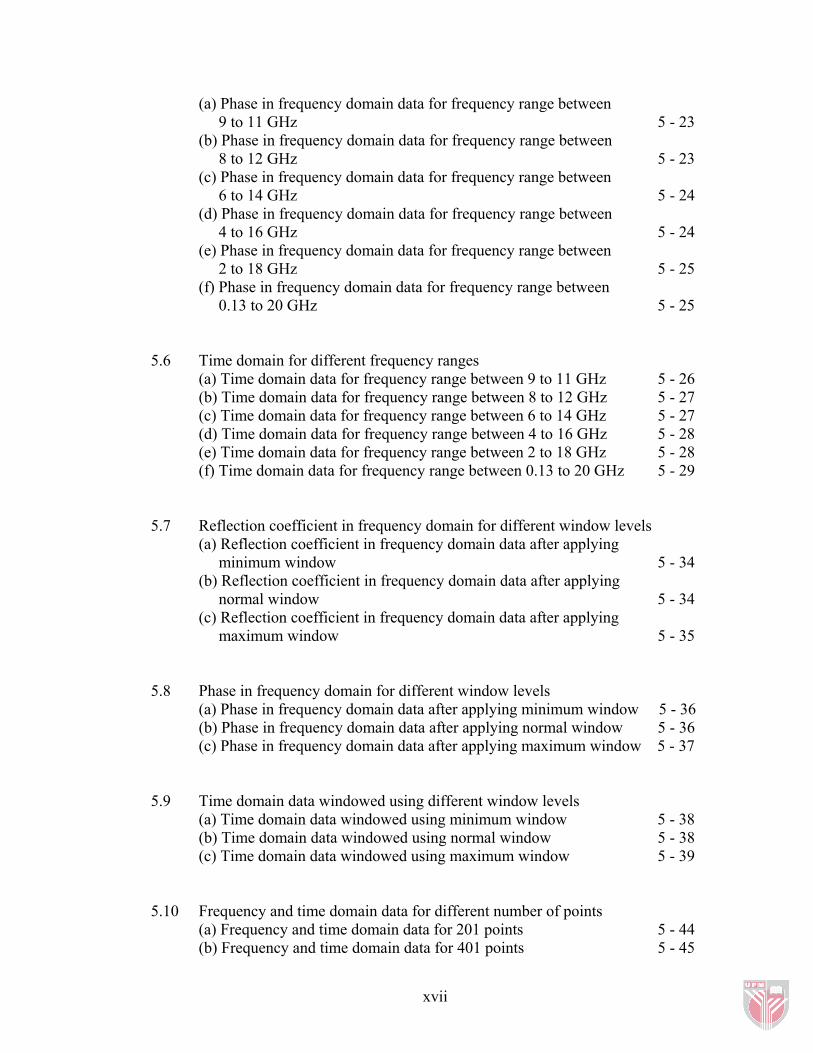
(a) Phase in frequency domain data for frequency range between 9 to 11 GHz 5 - 23 (b) Phase in frequency domain data for frequency range between 8 to 12 GHz 5 - 23 (c) Phase in frequency domain data for frequency range between 6 to 14 GHz 5 - 24 (d) Phase in frequency domain data for frequency range between 4 to 16 GHz 5 - 24 (e) Phase in frequency domain data for frequency range between 2 to 18 GHz 5 - 25 (f) Phase in frequency domain data for frequency range between 0.13 to 20 GHz 5 - 25

5.6 Time domain for different frequency ranges (a) Time domain data for frequency range between 9 to 11 GHz 5 - 26 (b) Time domain data for frequency range between 8 to 12 GHz 5 - 27 (c) Time domain data for frequency range between 6 to 14 GHz 5 - 27 (d) Time domain data for frequency range between 4 to 16 GHz 5 - 28 (e) Time domain data for frequency range between 2 to 18 GHz 5 - 28 (f) Time domain data for frequency range between 0.13 to 20 GHz 5 - 29

5.7 Reflection coefficient in frequency domain for different window levels (a) Reflection coefficient in frequency domain data after applying minimum window 5 - 34 (b) Reflection coefficient in frequency domain data after applying normal window 5 - 34 (c) Reflection coefficient in frequency domain data after applying maximum window 5 - 35

5.8 Phase in frequency domain for different window levels (a) Phase in frequency domain data after applying minimum window 5 - 36 (b) Phase in frequency domain data after applying normal window 5 - 36 (c) Phase in frequency domain data after applying maximum window 5 - 37

5.9 Time domain data windowed using different window levels (a) Time domain data windowed using minimum window 5 - 38 (b) Time domain data windowed using normal window 5 - 38 (c) Time domain data windowed using maximum window 5 - 39

5.10 Frequency and time domain data for different number of points (a) Frequency and time domain data for 201 points 5 - 44 (b) Frequency and time domain data for 401 points 5 - 45

xvii

(c) Frequency and time domain data for 801 points 5 - 46 (d) Frequency and time domain data for 1601 points 5 - 47

5.11 Frequency and time domain for different frequency ranges (a) Frequency and time domain data for frequency range between 9 to 11 GHz 5 - 52 (b) Frequency and time domain data for frequency range between 8 to 12 GHz 5 - 53 (c) Frequency and time domain data for frequency range between 6 to 14 GHz 5 - 54 (d) Frequency and time domain data for frequency range between 4 to 16 GHz 5 - 55 (e) Frequency and time domain data for frequency range between 2 to 18 GHz 5 - 56 (f) Frequency and time domain data for frequency range between 0.13 to 20 GHz 5 - 57

5.12 Frequency and time domain data for different setup configurations (a) Frequency and time domain data for setup A 5 - 60 (b) Frequency and time domain data for setup B 5 - 61 (c) Frequency and time domain data for setup C 5 - 62 (d) Frequency and time domain data for setup D 5 - 63 (e) Frequency and time domain data for setup E 5 - 64 (f) Frequency and time domain data for setup F 5 - 65 (g) Frequency and time domain data for setup G 5 - 66 (h) Frequency and time domain data for setup H 5 - 67 (i) Frequency and time domain data for setup I 5 - 68 (j) Frequency and time domain data for setup J 5 - 69

LIST OF ABBREVIATIONS

xviii

α attenuation constant in radians per unit length

β phase constant in radians per unit length

c velocity of light

D length

∆f the spacing between frequency data points

rε dielectric constant.

inE or incident voltage iE

rE reflected voltage

γ complex propagation constant

inI incident current

Γ reflection coefficient

| | magnitude reflection coefficient Γ

t two-trip time

fv velocity factor

vp velocity of propagation

ω angular velocity in radians per second

C capacitance

G admittance

L inductance

R resistance

T transit time from monitoring point to the

mismatch and back again

Zin input impedance

xix

Zo characteristic impedance

LZ load impedance

ADC Analog-to-Digital Converter

Agilent VEE Agilent Visual Engineering Environment

CZT Chirp z-transform

DC Direct Current

DFT Discrete Fast Fourier Transform

FDR Frequency Domain Reflectometry

FFT Fast Fourier Transform

HPIB Hewlett-Packard5 Interface Bus

IFFT Inverse Fast Fourier Transform

MATLAB Matrix Laboratory

RF Radio Frequency

SNR Signal-to-Noise Ratio

SWR Standing Wave Ratio

TDR Time Domain Reflectometry

VNA Vector Network Analyzer

VSWR Voltage Standing Wave Ratio

xx

CHAPTER 1

INTRODUCTION

Time Domain Reflectometry (TDR) is a remote sensing electrical measurement

technique that is nondestructive and has been used for many years to determine the

spatial location and nature of various objects. It is utilized to determine the

characteristics of transmission lines by observing reflected waveforms. It is an extension

of an earlier technique in which reflections from an electrical pulse were monitored to

locate faults/discontinuities and to determine the characteristics of power transmission

lines.

An early form of TDR that most people are familiar with is radar and was largely

developed as the result of World War II radar research. However, there is a lacked in

necessary instrumentation to make full use of TDR. With the advent of commercial TDR

research oscilloscopes in the early 1960's, it became feasible to test this new technology.

Today, TDR technology is the "cutting edge" methodology for many diverse

applications.

1.1 An Overview of the Determination of Material Discontinuities

Material discontinuity is defined as the tangible substance that goes into the makeup of a

physical object lacking in connection or continuity. Translating it into a more physical

term, it is the difference in impedance which causes a mismatch in connectivity or

continuity of the material or object under test or of measurement. In the following

subtopics the issue pertaining material discontinuities, its application and technology is

discussed.

Material discontinuity can take into many forms in the world of science and technology.

It is the change in electrical properties of a substance, the impedance difference or

mismatch in a material or simply a disconnected electrical wire or a change of chemical

property in a pure alloy.

In technological point of view, this can be applied to engineering, geographical and even

agricultural industry. For example, in engineering field, this analogy applies to fault

locating technique where faults in cable, cracks in pipes, walls of building and even

roads need to be detected to prevent further damage. In geographical field, the study of

terrain, archeological excavation and even vegetation area has a need in recognition

technique. For the agriculture industry, there is a need for moisture content measurement

for soil and even rubber milk. For a noninvasive and nondestructive testing technique,

the microwave method can be applied.

1 - 2

1.1.1 Technology and Application in Determination of Material Discontinuities

The TDR is widely used for its accuracy and is one of the many nondestructive testing

for locating fault. It transmits a fast rise time pulse along the conductor. If the conductor

is of uniform impedance and properly terminated, the entire transmitted pulse will be

absorbed in the far-end termination and no signal will be reflected back to the TDR.

However, where impedance discontinuities exist, each discontinuity will create an echo

that is reflected back to the reflectometer (hence the name). Increases in the impedance

create an echo that reinforces the original pulse while decreases in the impedance create

an echo that opposes the original pulse. The resulting reflected pulse measured at the

output/input to the TDR is displayed or plotted as a function of time and, since the speed

of signal propagation is relatively constant for a given transmission medium, can be read

as a function of cable length. This is similar in principle to radar.

Because of this sensitivity to impedance variations, a TDR is often used to verify cable

impedance characteristics, splice and connector locations and associated losses, and

estimate cable lengths, as every nonhomogenity in the impedance of the cable will

reflect some signal back in the form of echoes.

The TDR techniques have been utilized in many fields. It is used to determine soil

moisture water content in porous media, where over the last two decades substantial

advances have been made; including in soils, grains and food stuffs, and in sediments.

The key to TDR’s success is its ability to accurately determine the permittivity

1 - 3

(dielectric constant) of a material from wave propagation, and the fact that there is a

strong relationship between the permittivity of a material and its water content.

TDR has also been utilized to monitor slope movement in a variety of geotechnical

settings including highway cuts, rail beds, and open pit mines. In stability monitoring

applications using TDR, a coaxial cable is installed in a vertical borehole passing

through the region of concern. The electrical impedance at any point along a coaxial

cable changes with deformation of the insulator between the conductors. A brittle grout

surrounds the cable to translate earth movement into an abrupt cable deformation that

shows up as a detectable peak in the reflectance trace.

TDR equipment are commonly used for in-place testing of very long cable runs, where it

is impractical to dig up or remove what may be a kilometers-long cable. They are

indispensable for preventive maintenance of telecommunication lines, as they can reveal

growing resistance levels on joints and connectors as they corrode, and increasing

insulation leakage as it degrades and absorbs moisture long before either leads to

catastrophic failures. Using a TDR, it is possible to pinpoint a fault to within feet or

inches.

In labs and research centers, TDR technique is incorporated in measurement equipment

called ‘Vector Network Analyzer’ (VNA). It makes measurement by sweeping

frequencies over a device under test (DUT) and transforms it into time domain using the

time domain option available in the equipment.

1 - 4