time domain stability margin assessment · time domain stability margin assessment keith clements...

Time Domain Stability Margin Assessment

Keith Clements∗

The baseline stability margins for NASA’s Space Launch System (SLS) launch vehiclewere generated via the classical approach of linearizing the system equations of motionand determining the gain and phase margins from the resulting frequency domain model.To improve the fidelity of the classical methods, the linear frequency domain approachcan be extended by replacing static, memoryless nonlinearities with describing functions.This technique, however, does not address the time varying nature of the dynamics ofa launch vehicle in flight. An alternative technique for the evaluation of the stability ofthe nonlinear launch vehicle dynamics along its trajectory is to incrementally adjust thegain and/or time delay in the time domain simulation until the system exhibits unstablebehavior. This technique has the added benefit of providing a direct comparison betweenthe time domain and frequency domain tools in support of simulation validation.

Contents

I Background 2A Gain and Phase Explanation . . . . . . . . . . . . . . . . . . . . . . . . . . . . . . . . . . . . 2B Gain and Phase Margins . . . . . . . . . . . . . . . . . . . . . . . . . . . . . . . . . . . . . . . 3

II Introduction 5

IIIStability Margin Assessment Method 6A Rigid Body Gain Margin . . . . . . . . . . . . . . . . . . . . . . . . . . . . . . . . . . . . . . . 7B Rigid Body Phase Margin . . . . . . . . . . . . . . . . . . . . . . . . . . . . . . . . . . . . . . 8C Aero Gain Margin . . . . . . . . . . . . . . . . . . . . . . . . . . . . . . . . . . . . . . . . . . 9D Time Points Analyzed . . . . . . . . . . . . . . . . . . . . . . . . . . . . . . . . . . . . . . . . 10E Variables Assessed . . . . . . . . . . . . . . . . . . . . . . . . . . . . . . . . . . . . . . . . . . 10

IV Results 13

V Significant Findings 16A AAC Recovery of Gain-Unstable Systems . . . . . . . . . . . . . . . . . . . . . . . . . . . . . 16B Degradation Associated with Gimbal Limiting . . . . . . . . . . . . . . . . . . . . . . . . . . . 17C Aero Gain Margin Assessment . . . . . . . . . . . . . . . . . . . . . . . . . . . . . . . . . . . 20

VI Conclusions 21

∗Control System Analyst, ERC, Inc., Jacobs ESSSA Group, Huntsville, AL, [email protected]

1 of 22

American Institute of Aeronautics and Astronautics

https://ntrs.nasa.gov/search.jsp?R=20160013364 2020-03-18T21:37:20+00:00Z

I. Background

Before delving into the details of time domain stability margin assessment, an overview of the conceptsof gain and phase margin will be discussed.

A. Gain and Phase Explanation

A standard control system accepts an input signal, manipulates the signal in some way, then outputs theresult. During the manipulation of the input signal, the amplitude can potentially be modified. The ratioof the magnitude of the output/input signals is called the gain. The gain is often expressed in dB, which isdone by performing the operation: 20*log10(gain). Figure 1 below shows an example of what this would looklike. In this example, the ratio of the peaks is 2, so the gain is 2. The gain in dB would be 20*log(2) = 6.02 dB.

The output can also experience a ”lag” or ”delay” as a result of the manipulation of the input signal.This is known as the phase. The phase is usually expressed in degrees. This is done by finding the time de-lay induced by the control system (in seconds) and using the formula: phase = 360×frequency×delay. Figure2 below shows an example of a phase shift. The phase of the system in this example is 360(1/6.28)(-1.57) =-90◦.

Figure 1. Example of Gain

2 of 22


Figure 2. Example of Phase

B. Gain and Phase Margins

A physical system can have a number of uncertainties associated with it. For large systems (like a rocket),many uncertainties can arise. The gain margin dictates how much extra gain modification can occur before asystem goes unstable, and the phase margin is how much extra phase lag can occur before a system becomesunstable. An instability occurs when the gain of the system reaches 0 dB (or greater) at the same time thatthe phase reaches -180 degrees. The gain and phase margins are built into the system in order to preventinstabilities due to any modeling uncertainties when the real system is built (for SLS, minimum phase marginis 30 deg and minimum gain margin is 6 dB).

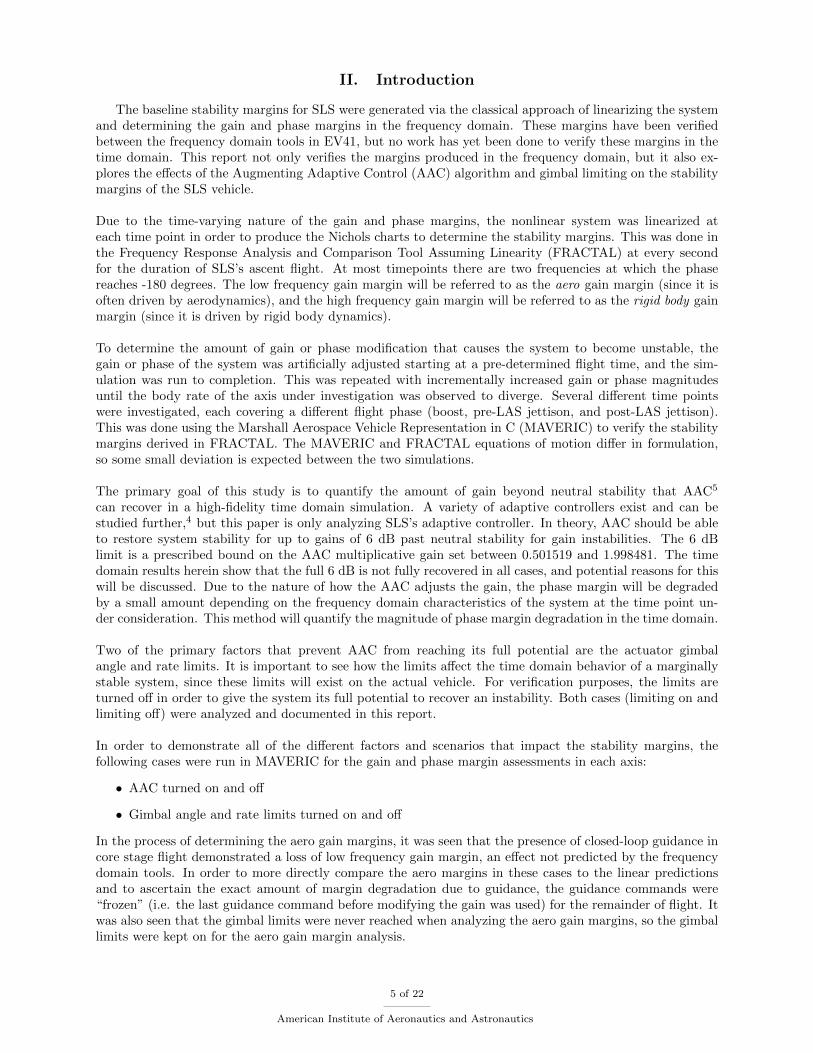
There are a few frequency-domain tools that can be used to identify these gain and phase margins. Twoof the most common are Bode Plots and Nichols Charts2 . A Bode plot consists of two plots: gain vs.frequency and phase vs. frequency. The gain margin is found by finding the frequency at which the phasereaches -180 degrees, then taking the negative of the gain value at that frequency. The phase margin is foundby finding the frequency at which the gain reaches 0 dB, then subtracting the corresponding phase at thatfrequency from 180 degrees. This is shown graphically in Figure 3 and more information can be found inthe references. The tool of choice in the Control Systems Design and Analysis Branch (EV41) at MSFC isthe Nichols Chart. This is simply a combination of the gain and phase components of the Bode Plot whichresults in a plot of gain vs. phase. The gain and phase margins can be easily found by finding the y andx intercepts of this plot, respectively. The “crossover frequency” will be used to convert time delays to aphase degradation in this paper. This is the frequency at which the gain reaches 0 dB (the frequency usedfor calculating the phase margin).

An example of a simulated system, 100s3+11s2+38s+40 vs. a real system, 150

s3+10s2+27s+18 is shown in Figures3 and 4. The gain and phase margins are highlighted on each of these plots. The “real” and “simulated”curves illustrate the importance of building in the gain and phase margins to the control system design. Ifthe difference between the simulated model and the real system are different enough, an instability has thepotential to occur in the real system.

3 of 22


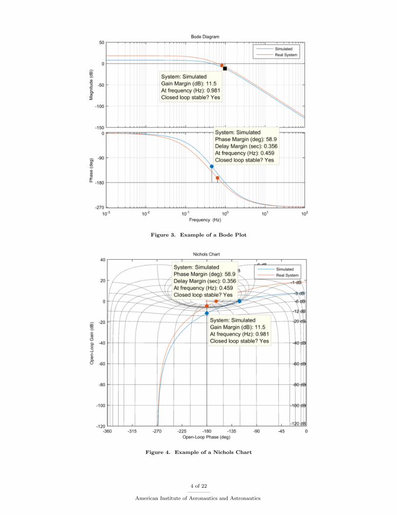
Figure 3. Example of a Bode Plot

Figure 4. Example of a Nichols Chart

4 of 22


II. Introduction

The baseline stability margins for SLS were generated via the classical approach of linearizing the systemand determining the gain and phase margins in the frequency domain. These margins have been verifiedbetween the frequency domain tools in EV41, but no work has yet been done to verify these margins in thetime domain. This report not only verifies the margins produced in the frequency domain, but it also ex-plores the effects of the Augmenting Adaptive Control (AAC) algorithm and gimbal limiting on the stabilitymargins of the SLS vehicle.

Due to the time-varying nature of the gain and phase margins, the nonlinear system was linearized ateach time point in order to produce the Nichols charts to determine the stability margins. This was done inthe Frequency Response Analysis and Comparison Tool Assuming Linearity (FRACTAL) at every secondfor the duration of SLS’s ascent flight. At most timepoints there are two frequencies at which the phasereaches -180 degrees. The low frequency gain margin will be referred to as the aero gain margin (since it isoften driven by aerodynamics), and the high frequency gain margin will be referred to as the rigid body gainmargin (since it is driven by rigid body dynamics).

To determine the amount of gain or phase modification that causes the system to become unstable, thegain or phase of the system was artificially adjusted starting at a pre-determined flight time, and the sim-ulation was run to completion. This was repeated with incrementally increased gain or phase magnitudesuntil the body rate of the axis under investigation was observed to diverge. Several different time pointswere investigated, each covering a different flight phase (boost, pre-LAS jettison, and post-LAS jettison).This was done using the Marshall Aerospace Vehicle Representation in C (MAVERIC) to verify the stabilitymargins derived in FRACTAL. The MAVERIC and FRACTAL equations of motion differ in formulation,so some small deviation is expected between the two simulations.

The primary goal of this study is to quantify the amount of gain beyond neutral stability that AAC5

can recover in a high-fidelity time domain simulation. A variety of adaptive controllers exist and can bestudied further,4 but this paper is only analyzing SLS’s adaptive controller. In theory, AAC should be ableto restore system stability for up to gains of 6 dB past neutral stability for gain instabilities. The 6 dBlimit is a prescribed bound on the AAC multiplicative gain set between 0.501519 and 1.998481. The timedomain results herein show that the full 6 dB is not fully recovered in all cases, and potential reasons for thiswill be discussed. Due to the nature of how the AAC adjusts the gain, the phase margin will be degradedby a small amount depending on the frequency domain characteristics of the system at the time point un-der consideration. This method will quantify the magnitude of phase margin degradation in the time domain.

Two of the primary factors that prevent AAC from reaching its full potential are the actuator gimbalangle and rate limits. It is important to see how the limits affect the time domain behavior of a marginallystable system, since these limits will exist on the actual vehicle. For verification purposes, the limits areturned off in order to give the system its full potential to recover an instability. Both cases (limiting on andlimiting off) were analyzed and documented in this report.

In order to demonstrate all of the different factors and scenarios that impact the stability margins, thefollowing cases were run in MAVERIC for the gain and phase margin assessments in each axis:

• AAC turned on and off

• Gimbal angle and rate limits turned on and off

In the process of determining the aero gain margins, it was seen that the presence of closed-loop guidance incore stage flight demonstrated a loss of low frequency gain margin, an effect not predicted by the frequencydomain tools. In order to more directly compare the aero margins in these cases to the linear predictionsand to ascertain the exact amount of margin degradation due to guidance, the guidance commands were“frozen” (i.e. the last guidance command before modifying the gain was used) for the remainder of flight. Itwas also seen that the gimbal limits were never reached when analyzing the aero gain margins, so the gimballimits were kept on for the aero gain margin analysis.

5 of 22


III. Stability Margin Assessment Method

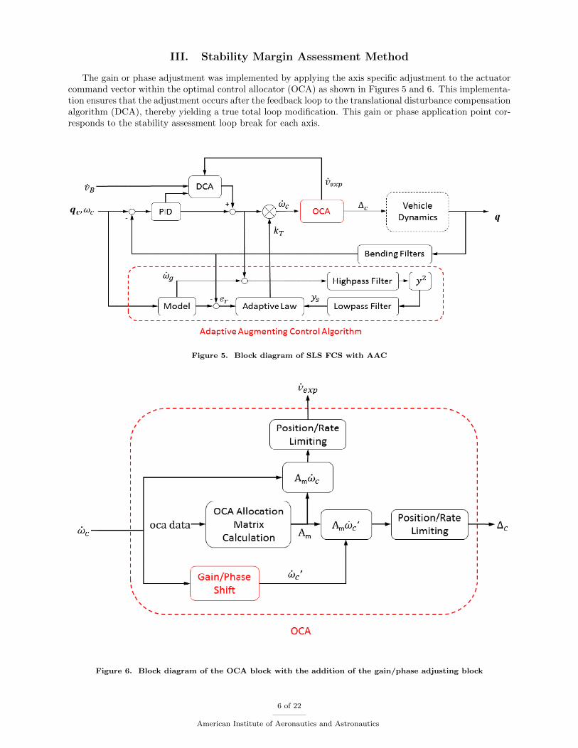
The gain or phase adjustment was implemented by applying the axis specific adjustment to the actuatorcommand vector within the optimal control allocator (OCA) as shown in Figures 5 and 6. This implementa-tion ensures that the adjustment occurs after the feedback loop to the translational disturbance compensationalgorithm (DCA), thereby yielding a true total loop modification. This gain or phase application point cor-responds to the stability assessment loop break for each axis.

Figure 5. Block diagram of SLS FCS with AAC

Figure 6. Block diagram of the OCA block with the addition of the gain/phase adjusting block

6 of 22


A. Rigid Body Gain Margin

Using the time history of stability margins derived from the baseline linearization approach, the time do-main derived stability margins were determined via multiple time domain simulations in which axis-specificincremental gain adjustments were made to the nominal system about the expected neutral stability point.The baseline stability margin time histories were used to shift the gain up to the frequency-domain valuesaround the zero margin point such that a precise amount of expected instability was maintained throughoutflight. When assessing the gain margins, the gain was applied starting at the time point under consideration,thereafter following the variation in the margin found in the linear analysis. Figure 7 shows an example ofthe incremental gain application, and Figure 8 shows an array of time domain simulations for the exampletime point. Note: numbers on many of the plots in this report were deleted in order to comply with ITARregulations. The general trends can be used to understand the concepts.

Figure 7. Example of the applied gains in the time domain

7 of 22


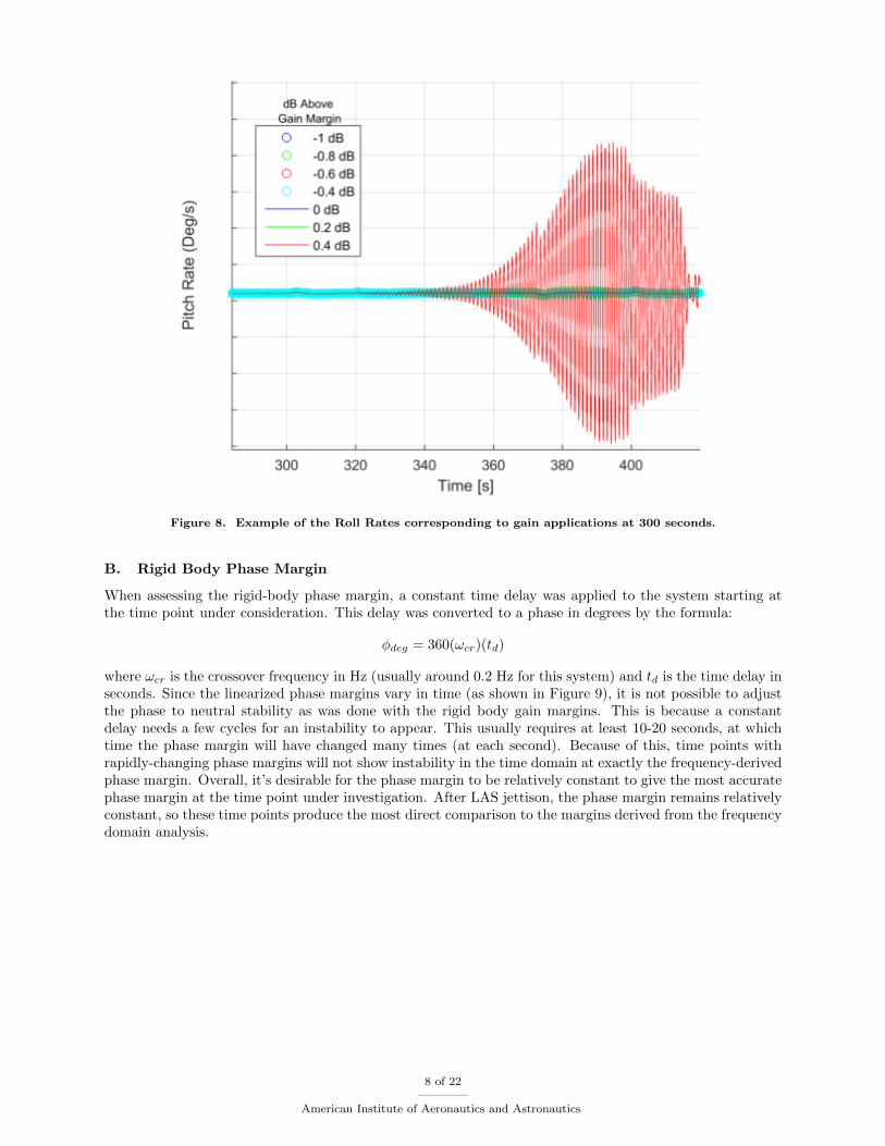
Figure 8. Example of the Roll Rates corresponding to gain applications at 300 seconds.

B. Rigid Body Phase Margin

When assessing the rigid-body phase margin, a constant time delay was applied to the system starting atthe time point under consideration. This delay was converted to a phase in degrees by the formula:

φdeg = 360(ωcr)(td)

where ωcr is the crossover frequency in Hz (usually around 0.2 Hz for this system) and td is the time delay inseconds. Since the linearized phase margins vary in time (as shown in Figure 9), it is not possible to adjustthe phase to neutral stability as was done with the rigid body gain margins. This is because a constantdelay needs a few cycles for an instability to appear. This usually requires at least 10-20 seconds, at whichtime the phase margin will have changed many times (at each second). Because of this, time points withrapidly-changing phase margins will not show instability in the time domain at exactly the frequency-derivedphase margin. Overall, it’s desirable for the phase margin to be relatively constant to give the most accuratephase margin at the time point under investigation. After LAS jettison, the phase margin remains relativelyconstant, so these time points produce the most direct comparison to the margins derived from the frequencydomain analysis.

8 of 22


Figure 9. FRACTAL baseline phase margins

C. Aero Gain Margin

The baseline stability margin time histories were used to shift the gain down to various values around thezero margin point such that a precise amount of expected instability was maintained throughout flight.When assessing the aero gain margins, the gain was applied starting at the time point under consideration,thereafter following the variation in the margin found in the linear analysis. Figure 10 shows the baselinemargins FRACTAL. Due to the quickly varying nature of the boost phase aero gain margin and the muchslower time constant of the corresponding instability, initial attempts at identifying the aero margin in boostphase proved inconclusive. Only aero gain margins in the core stage of flight after SRB separation aredocumented herein. Note that in this exo-atmospheric region of flight, the aero margin not actually definedby aerodynamics but by other more constant system dynamics and so is sometimes referred to as the “lowfrequency gain margin”.

9 of 22


Figure 10. FRACTAL Baseline Aero Gain Margins

D. Time Points Analyzed

The time domain simulations were repeated for several operating points and for a range of gain and phaseoffsets in the vicinity of the expected margins found from the linear analysis. The operating points werechosen to assess the three main phases of flight. The operating points were at 70 seconds during boost stageflight, 140 seconds (for phase and aero gain margins only), 180 sec (for rigid body gain margins only), and300 seconds during core stage flight after LAS jettison. These were chosen to capture the dynamics of eachflight regime.

For each time point, the gain was varied in 0.2 dB steps, and the delay was applied in 0.02 second in-crements (50 Hz frame delay). For each time point, the stability margin was found through a numericalassessment of the time domain results. The metrics and method for assessment of instability depends uponthe type of stability margin being verified and the configuration of the system.

E. Variables Assessed

In order to determine the first simulation that displays unstable behavior, a set of variables was createdto fully assess the instabilities. The legend of the gain margin figures shown below show the magnitude ofinstability, that is, the amount beyond the gain margin for the time point under consideration. This formatwill be used for the gain margin differences throughout this report.

• Body Rates (p, q, or r): These are the main indicators of instability. If the axis under investigationdisplays divergent oscillations in its body rate, it is said to be unstable. Figure 11 shows an exampleof the roll rate during an instability applied to the x-axis. It is clear that the first unstable case is4.6 dB above neutral stability as shown by the diverging roll rate. The body rate in the axis underinvestigation is the primary variable for determining stability, so this is always the deciding factor indetermining the first unstable simulation. The variables were evaluated manually by finding the firstsimulation to show a truly diverging body rate.

10 of 22


• Max engine saturation ratio: This variable measures the maximum of the ratio of the commandedgimbal angles to that of the actual gimbal angles. If the max engine saturation ratio is larger thanone, the system has reached gimbal angle saturation. For cases with gimbal limits enabled, this willlikely lead to an instability. For cases with gimbal limits off, divergent behavior of this variable isindicative of an instability. Figure 12 shows an example of the max engine saturation ratio variablethat corresponds to the instability in Figure 11.

• Adaptive Gain: For cases with AAC enabled, this variable is a good indicator of instability. If theadaptive gain is saturated (either 2.0 or 0.5), it is no longer improving the performance of the system.If this is the case for long enough (usually about 10-15 seconds), the system will often become unstable.Although this is not always the instability point, it is a good way to hone in on the instability pointwhen looking at vehicle dynamics. Figure 13 shows an example of the adaptive gain associated with theinstability in Figure 11. It is easy to see that the first unstable case is 4.6 dB above neutral stability,since that is the first simulation that shows saturation in the adaptive gain.

Figure 11. Roll Rate for Rigid Body Gain Adjustments Applied at 300 seconds (Limits On, AAC On)

11 of 22


Figure 12. Engine Saturation Ratio for Rigid Body Gain Adjustments Applied at 300 seconds (Limits On,AAC On)

Figure 13. Roll Adaptive Gain for Rigid Body Gain Adjustments Applied at 300 seconds (Limits On, AACOn)

12 of 22


IV. Results

The method described in the previous section was applied to the 4 configurations in which AAC wasenabled or disabled and limits to gimbal angle and rate commands issued by the controller were enabled ordisabled. Note that the cases with the gimbal limits disabled were only used to assess rigid gain and phasemargin as the aero gain margin cases were observed in all cases to avoid control saturation.

Since AAC is expected to increase gain margins by 6 dB, the baseline gain margin with AAC enabledare the same curves as with AAC disabled but with an additional 6 dB. There is no exact expected shift inphase margin with AAC enabled; therefore, only the baseline phase margin with AAC disabled is shown inthese figures.

When AAC is disabled, the stability margins demonstrate close agreement between the time domain sim-ulations and the linear predictions. This match provides credibility to the methods and tools used addingsignificant confidence in the basic flight control design. While the tabular results show discrepancies betweenthe baseline and time domain derived phase margins during boost stage, this can be attributed to the rapidvariation in phase margin during the highly dynamic region of flight.

With AAC enabled, the gain margins are always increased, the extent limited by various factors madeevident in the sections that follow. The systems with phase margins near neutral stability were found todemonstrate some degradation when AAC was enabled. This expected consequence of AAC, the context forits acceptance, and the exact extent of degradation will be provided in the following results.

Figure 14 shows the rigid body gain margins in the time domain. It is clear that AAC adds extra gainmargin to the system. It can also be seen that the gimbal limits constrain any additional amount of rigidbody gain margin provided by the inclusion of AAC, especially in core phase.

Figure 15 shows the rigid phase margins in the time domain. For many of the time points with AACoff, additional phase lag (time delay) beyond the linear prediction of neutral stability was required to showinstability. However, the majority of time points with AAC enabled experience a degraded phase margin.The magnitude of this effect is a function of the shape of the Nichols chart. In general, it can be seen thatthe limiting doesn’t affect these margins as much as the rigid body gain margins since the slowly divergingnature of the instabilities takes time to reach command saturation. During boost phase, the phase marginsare changing very quickly. Because it takes at least 10-20 seconds for a phase instability to be realized in thetime domain, the margins calculated in the time domain can be significantly different from those calculatedin the frequency domain.

Figure 16 below shows the aero gain margins in the time domain, with guidance commands frozen startingat the time point under consideration. Due to the low magnitude and low frequency nature of these insta-bilities, it was difficult to determine the exact magnitude of each aero gain instability. With this in mind,the results below show that AAC increases the aero gain margin over the entire flight regime.

13 of 22


Figure 14. Time domain derived rigid gain margins

Figure 15. Time domain derived phase margins

14 of 22


Figure 16. Time domain derived aero gain margins

Tables 1 and 2 below show the data in the previous figures in tabular form. Note that the phase marginsare omitted to comply with ITAR regulations.

Table 1. Time Domain Derived Stability Margins – AAC Disabled

Margin Axis LimitsTime (sec)

70 140 180 300

Rigid Gain Margin Difference(dB)

RollOn 0.2 - 0 0

Off 0 - 0 0

PitchOn 0.2 - 0 -0.2

Off 0 - 0 -0.2

YawOn 0.2 - 0.2 0

Off 0.2 - 0 0

Aero Gain Margin Difference (dB)

Roll Off N/A -1 - 0.8

Pitch Off N/A 2 - 2

Yaw Off N/A -1 - 0.8

15 of 22


Table 2. Time Domain Derived Stability Margins – AAC Enabled

Margin Axis LimitsTime (sec)

70 140 180 300

Rigid Gain Margin Difference(dB)

RollOn 3.2 - 4.6 4.6

Off 4.6 - 3.6 5.8

PitchOn 4.2 - 3 4.8

Off 4.6 - 3.8 6

YawOn 3.8 - 4.4 4.6

Off 5 - 3.6 6

Aero Gain Margin Difference (dB)

Roll Off N/A 7 - 2

Pitch Off N/A 7 - 2

Yaw Off N/A 7 - 4.4

V. Significant Findings

A. AAC Recovery of Gain-Unstable Systems

A primary goal of this study was to observe the ability of AAC to recover gain-unstable systems. Across allcases tested, the gain margins from instability was increased by at least 4 dB in the MAVERIC time domain.Figures 17 - 18 show an example of AAC recovering the full 6 dB of rigid gain margin.

Figure 17. Pitch Body Rate for Rigid Body Gain Adjustments Applied at 300 seconds (Limits Off, AAC Off)

16 of 22


Figure 18. Pitch Body Rate for Rigid Body Gain Adjustments Applied at 300 seconds (Limits Off, AAC On)

B. Degradation Associated with Gimbal Limiting

Intuitively, it makes sense that a system will become unstable at lower magnitudes of gain or phase degra-dation if limits are applied to the command gimbal angles and command gimbal rates than it would if therewere no limits applied. An example of this can be seen in figures 18 and 19. In Figure 18, the system hasno limits applied, and it recovers the full 6 dB of gain margin; however, in Figure 19, limits are applied, andthe system only recovers 4.8 dB of gain margin.

17 of 22


Figure 19. Pitch Body Rate for Gain Adjustments Applied at 300 seconds (Limits On, AAC On)

The degradation associated with limiting is almost exclusively seen in the rigid body gain instabilities.This is likely due to the rapid divergence of these instabilities resulting from the low damping of the controlresponse near its second phase crossover. In some cases, the rigid phase margins are slightly affected by thegimbal limiting, but most cases show little to no degradation owing primarily to the very lightly dampedresponse of the system without phase margin. For example, Figures 20 - 21. The two plots show very littlevariation because the gimbal limits are rarely reached in the presence of the phase instabilities.

18 of 22


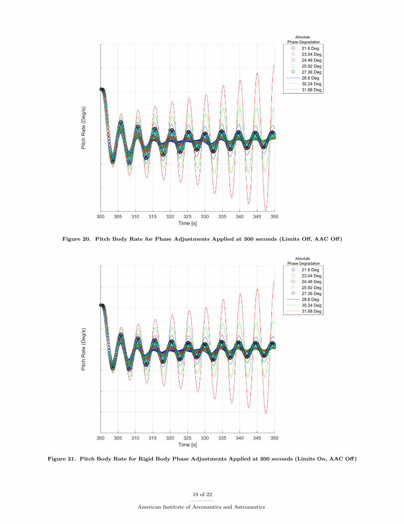
Figure 20. Pitch Body Rate for Phase Adjustments Applied at 300 seconds (Limits Off, AAC Off)

Figure 21. Pitch Body Rate for Rigid Body Phase Adjustments Applied at 300 seconds (Limits On, AAC Off)

19 of 22


C. Aero Gain Margin Assessment

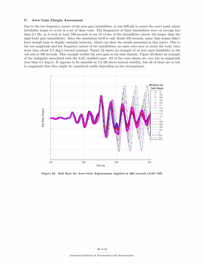
Due to the low frequency nature of the aero gain instabilities, it was difficult to assess the exact point whereinstability began to occur in a lot of these tests. The frequencies of these instabilities were on average lessthan 0.1 Hz, so it took at least 100 seconds to see 10 cycles of the instabilities (about 10x longer than therigid body gain instabilities). Since the simulation itself is only about 450 seconds, many time points didn’thave enough time to display unstable behavior, which can skew the results presented in this report. Due tothe low amplitude and low frequency nature of the instabilities, no cases were seen to excite the body ratesmore than about 0.5 deg/s beyond nominal. Figure 22 shows an example of an aero gain instability in theroll axis at 300 seconds. This example verifies the aero gain in the time domain. Figure 23 shows an exampleof the ambiguity associated with the AAC enabled cases. All of the cases shown are very low in magnitude(less than 0.1 deg/s). It appears to be unstable at 5.2 dB above neutral stability, but all of these are so lowin magnitude that they might be considered stable depending on the circumstance.

Figure 22. Roll Rate for Aero Gain Adjustments Applied at 300 seconds (AAC Off)

20 of 22


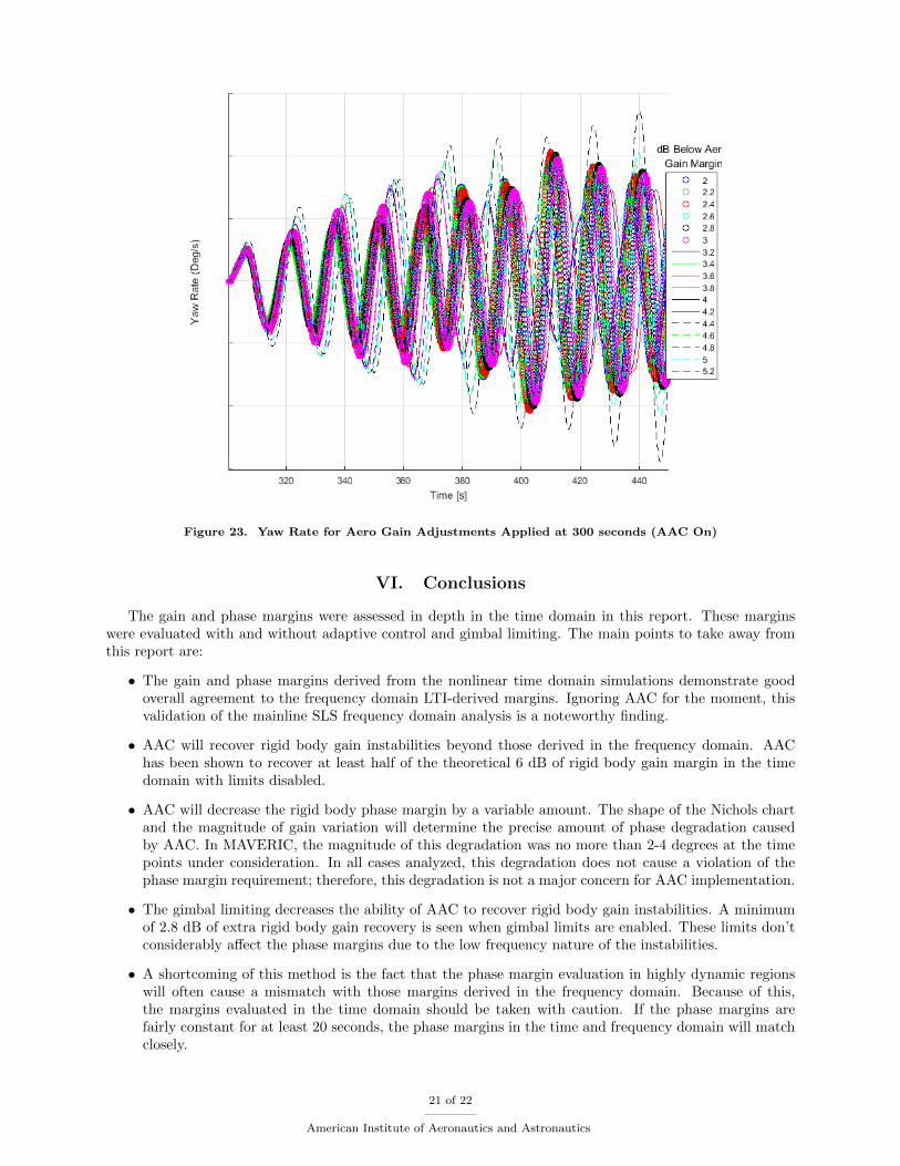
Figure 23. Yaw Rate for Aero Gain Adjustments Applied at 300 seconds (AAC On)

VI. Conclusions

The gain and phase margins were assessed in depth in the time domain in this report. These marginswere evaluated with and without adaptive control and gimbal limiting. The main points to take away fromthis report are:

• The gain and phase margins derived from the nonlinear time domain simulations demonstrate goodoverall agreement to the frequency domain LTI-derived margins. Ignoring AAC for the moment, thisvalidation of the mainline SLS frequency domain analysis is a noteworthy finding.

• AAC will recover rigid body gain instabilities beyond those derived in the frequency domain. AAChas been shown to recover at least half of the theoretical 6 dB of rigid body gain margin in the timedomain with limits disabled.

• AAC will decrease the rigid body phase margin by a variable amount. The shape of the Nichols chartand the magnitude of gain variation will determine the precise amount of phase degradation causedby AAC. In MAVERIC, the magnitude of this degradation was no more than 2-4 degrees at the timepoints under consideration. In all cases analyzed, this degradation does not cause a violation of thephase margin requirement; therefore, this degradation is not a major concern for AAC implementation.

• The gimbal limiting decreases the ability of AAC to recover rigid body gain instabilities. A minimumof 2.8 dB of extra rigid body gain recovery is seen when gimbal limits are enabled. These limits don’tconsiderably affect the phase margins due to the low frequency nature of the instabilities.

• A shortcoming of this method is the fact that the phase margin evaluation in highly dynamic regionswill often cause a mismatch with those margins derived in the frequency domain. Because of this,the margins evaluated in the time domain should be taken with caution. If the phase margins arefairly constant for at least 20 seconds, the phase margins in the time and frequency domain will matchclosely.

21 of 22


• Another shortcoming of this method is that fact that it is difficult to pinpoint the exact magnitudeof instability when assessing the aero gain margins. Because of this, the aero gain margins presentedin this report should be taken with some uncertainty. In any case, the magnitude and frequency ofthese instabilities is very low; therefore, the instabilities will not have a significant effect on missionperformance and objectives.

Acronyms

AAC Augmenting Adaptive ControlDCA Disturbance Compensation AlgorithmFCS Flight Control SystemFRACTAL Frequency Response Analysis and Comparison Tool Assuming LinearityLAS Launch Abort SystemMAVERIC Marshall Aerospace VEhicle Representation in CMSFC Marshall Space Flight CenterOCA Optimal Control AllocatorSLS Space Launch System

Acknowledgments

Thanks to John Wall and the EV41 controls team for help with several technical aspects of this report.Thanks to Tannen VanZwieten and the NESC team at MSFC for giving detailed feedback on the results ofthis report.

References

1Brogan, William L,Modern Control Theory, 3rd Edition, 1991.2Nise, Norman, Control Systems Engineering, Wiley Publishing, Chesapeake, 2015.3Orr, Jeb S., Wall, John H., and VanZwieten, Tannen; Space Launch System Ascent Flight Control Design, 2013.4Ioannou, Petros, Sun, Jing Robust Adaptive Control, Dover, 2012.5Wall, John H., Orr, Jeb S., and VanZwieten, Tannen; Space Launch System Implementation of Adaptive Augmenting

Control, AAS 2014.

22 of 22


time domain stability margin assessment · time domain stability margin assessment keith clements...

Documents