Time Evolution of States for Open Quantum Systems.

The quadratic case∗

Didier Robert

Abstract

Our main goal in this paper is to extend to any system of coupled quadratic Hamiltonianssome properties known for systems of quantum harmonic oscillators related with the BrownianQuantum Motion model. In a first part we get a rather general formula for the purity (or thelinear entropy) in a short time approximation. For this formula the quadratic assumption is notnecessary, more general Hamiltonians can be considered.In a second part we establish a master equation (or a Fokker-Planck type equation) for thetime evolution of the reduced matrix density for bilinearly coupled quadratic Hamiltonians. TheHamiltonians and the bilinear coupling can be time dependent.Moreover we give an explicit formula for the solution of this master equation so that the timeevolution of the reduced density at time t is written as a convolution integral for the reduceddensity at initial time t0 = 0, with a Gaussian kernel, for 0 ≤ t < tc where tc ∈]0,∞] is a criticaltime. Reversibility is lost for t ≥ tc.

1 Introduction

The general setting considered here is a quantum system (S) interacting with an environment (E). Thetotal system (S)∪(E) is supposed to be an isolated quantum system and we are interested in dynamicalproperties of (S) alone, which is an open system because of its interactions with (E). In particularduring the time evolution the energy of (S) is not preserved and its evolution is not determined by aSchrodinger or Liouville-von Neumann equation unlike for the total system (S) ∪ (E).The Hilbert space of the total system (S)∪(E) is the tensor productH = HS⊗HE i and its HamiltonianH is decomposed as follows:

H = HS ⊗ I + I⊗ HE︸ ︷︷ ︸H0

+HI = H0 + V (1.1)

(S)∪(E) is isolated by assumption and its evolution obeys the Schrodinger (or Liouville-von Neumann)equation with the Hamiltonian H.All Hamiltonians here are self -adjoint operators on their natural domain, H and HI = V are definedin H, HS in HS , HE in HE . Moreover most of the results stated here are valid when the Hamiltoniansare time dependent, assuming that their propagators exist as unitary operators in the correspondingHilbert space.Quantum observables are denoted with a hat accent, the corresponding classical observables (alsonamed Wigner function or Weyl-symbols) are written by erasing the hat.We don’t give here more details concerning the domains, these will be clear in the applications.

∗This work was supported by the French Agence Nationale de la Recherche, NOVESOL project, ANR 2011,BS0101901

iWhen the spaces are infinite dimensional we mean here that HS ⊗HE is the Hilbert tensor product (completion ofthe algebraic tensor product).

1

2

We assume that the interacting potential V has the following form

V =∑

1≤j≤m

Sj ⊗ Ej (1.2)

where Sj and Ej are self-adjoint operators in HS , HE respectively.Recall that a density matrix ρ is a positive class trace operator with trace one (trρ = 1). ρ is a

state of the total system (S)∪ (E) in the Hilbert space H. The time evolution of ρ obeys the followingLiouville-von Neumann equation:

˙ρ = i−1[H, ρ], ρ : t 7→ ρ(t) (1.3)

Time derivatives are denoted by a dot, [·, ·] denotes the commutator of two observables.We assume that for t = 0 the system and the environment are decoupled :

ρ(0) = ρS(0)⊗ ρE(0), ρS,E(0) are density matrices in HS,E (1.4)

and the state ρS(0) of the system is pure i.e is an orthogonal projector on a unit vector ψ of HS . Anon pure state will be called a mixed state. A density matrix ρS is a mixed state if and only if ρS hasan eigenvalue λ, such that 0 < λ < 1.If ρ is a pure state then ρ = Πψ, ψ ∈ H, ‖ψ‖ = 1 where Πψ(η) = 〈ψ, η〉ψ.

The general problem for open systems is to describe the evolution ρS(t) of the density matrix of thesystem (S). In particular an important physical question is: when the state ρS(t) is pure or mixed?To decide if a state is pure or not we consider the purity function

pur(t) = trS(ρS(t)2)

The function S`(t) = 1 − pur(t) is called the linear entropy. The Boltzman-von Neumann entropy isSBN = −trS(ρS log ρS).We clearly have 0 ≤ pur(t) ≤ 1. It is not difficult to see that ρS(t) is pure if and only if pur(t) = 1.With our assumption, 0 is a maximum for pur so we have pur(0) ≤ 0 and if pur(0) < 0 then for0 < t < ε, ρS(t) is a mixed state for ε small enough.For isolated (closed) systems, if the initial state is pure then it stays pure at every time, as it can beeasily seen using equation (1.3).So our first step in this paper is to compute pur(0). In particular for a large class of models, includingthe Quantum Brownian Motion, we shall prove that pur(0) < 0 so for these models the state of thesystem becomes very quickly decoherent and entangled with the environment.Our second goal is to compute the time evolution ρS(t) of the state of the system. We know thatρS(t) does not satisfy a Liouville- von Neumann equation because the system is open.We shall prove that for any time dependent quadratic systems, ρS(t) obeys an exact ”master equation”similar to a Fokker-Planck type equation, with time dependent coefficients, and from this equationwe can get an explicit formula for ρS(t).This could be a first step for more general systems in the semi-classical regime .

Let us recall a mathematical definition for ρS(t) and related properties and notations.This can be done by introducing partial trace (or relative trace) over the environment for a state ρ ofthe global system.

Definition 1.1 Let A be a class-trace operator in HS ⊗HE. We denote trEA the unique trace-classoperator on HS satisfying, for every bounded operator B on HS,

trS

((trEA)B

)= tr

(A(B ⊗ IE)

)(1.5)

3

We have denoted “tr” the trace in the total space H, trS,E the trace in HS,E respectively.

Of course we have the ”Fubini property”: trS(trEA) = trA. Moreover trE(B ⊗ C) = B · (trEC) if Band C are trace class operators in HS and HE respectively.If ρ is a density matrix in H then trE ρ is a density matrix in HS , called the reduced density matrixor the reduced state.From (1.5) we can compute the matrix element of trEA by the formula

〈ψ, (trEA)ϕ〉 = tr(A(Πψ,ϕ ⊗ IE)

), ∀ψ,ϕ ∈ HS .

The partial trace was introduced in quantum mechanics to explain quantum phenomena like entan-glement and decoherence (see [19, 20] for more details).

Let Ψ ∈ HS⊗HE , Ψ =∑

1≤j≤N

ψj ⊗ ηj . Ψ is a pure state in H = HS⊗HE . Let us compute the partial

trace of ΠΨ in HE . Applying Definition 1.1 we easily get

trE(ΠΨ) =∑

1≤j,k≤N

〈ηj , ηk〉Πψj ,ψk (1.6)

where Πψj ,ψk is the rank one operator in HS : Πψj ,ψk(ϕ) = 〈ψj , ϕ〉ψk.Decoherence means in particular that there exists a (non-orthonormal) basis ηj such that |〈ηj , ηk〉|becomes very small for j 6= k, so that trE(ΠΨ) is very close to

∑1≤j≤N

pjΠψj (pj = 〈ηj , ηj〉) hence

quantum interferences for the system (S) are lost.Formula (1.5) is an operator version of Fubini integration theorem as we can see in the Weyl quanti-zation setting.Let HS = L2(Rd) , HE = L2(RN ). Denote z = (x, ξ) ∈ R2d, u = (y, η) ∈ R2N , A = σwA the Weylsymbol of A in the Schwartz space S(R2(d+N)) (see [6] for more details) then the Weyl symbol of trEAis

σw(trEA)(z) = (2π)−N∫R2N

A(z, u)du. (1.7)

Our main applications here concern the Weyl-quadratic case where :

• HS , HE are quadratic Hamiltonians (generalized harmonic oscillators) respectively in the phasespaces R2d, R2N .

• HS , HE are quantum Hamiltonians (Weyl quantization of HS respectively HE) in L2(Rd) re-spectively L2(RN ).

• ρS is the projector on ψ ∈ S(Rd).

• ρE is a Gaussian with 0 means.

• Sj resp. Ej are linear forms on R2d resp. R2N (bilinear coupling).

In applications one consider thermal equilibrium states for environment: ρE = Z(β)−1e−βKE where

KE is a quadratic form, positive-definite and β = 1T , T > 0 is the temperature, Z(β) = tr(e−βKE ).

In this setting it is possible to find the exact time dependent master equation satisfied by ρS(t), as weshall see in the second part of this paper (ρE can be any environment state) and to solve this equationwhen the classical dynamics of the total system (S) ∪ (E) is known.

Let us remark that there exists a general formula, called Kraus formula, giving the time evolution

of the reduced system: ρS(t) = trE(U(t)ρ(0)U∗(t)) where ρ(0) = ρS(0)⊗ ρE(0) and U(t) = e−itH (see[20, 3]):

ρS(t) =∑j,`

Kj,`(t)ρS(0)Kj,`(t)∗ (1.8)

where the Kraus operators Kj,`(t) depends on ρE(0 and U(t). But the operators Kj,`(t) are notexplicitly known, so formula (1.8) is not easy to use to get properties of ρS(t).

4

2 A general computation

Our goal in this section is to give a local formula in time for the purity when the system (S) is in apure state.

It is easier here to consider the interaction formulation of quantum mechanics to ”eliminate” the

”free” (non-interacting) evolution: U0(t) = e−itH0 . In this section we consider the general settingdescribed in the introduction. In particular we assume that the interaction Hamiltonian V has theshape (1.2). As it is well known the time evolution (1.3) is given by the Schrodinger evolution

ρ(t) = U(t)ρ(0)U(t)∗, U(t) = e−itH .

For simplicity we assume here that all Hamiltonians are time independent but the results are alsovalid if H,Sj , Ej are time dependent. In this case we have U(t) = U(t, 0) where 0 is the initial time.Some technical assumptions are necessary to get rigorous results.

Let us denote Sp(H) the Schatten class of linear operators in the HilbertH such that∑j≥1

λj(|A|)p < +∞,

where |A| = (A∗A)1/2 and λj(|A|) is the eigenvalues series of |A|. For properties of Schatten classessee [14]. In particular S1(H) is the trace class space and S2(H) is the Hilbert-Schmidt space. Ourgeneral assumptions are the following.(GSE). There exist self-adjoint operators in H, K0 and K1 such that K1 is bounded, K0 is positivewith a bounded inverse K−1

0 in the Hilbert-Schmidt space S2(H) and such that

ρ(0) = K−10 K2

1K−10 .

(Ham)k. For all j ≤ k (k ∈ N), HjK−10 is in the Hilbert-Schmidt space S2(H).

Lemma 2.1 If assumptions (GSE) and (Ham)k are satisfied then t 7→ ρ(t) is Ck smooth in time t,from R into the trace class Banach space S1(H)

The proof is standard and is left to the reader.It is easier here to consider the interaction formulation of quantum mechanics to ”eliminate” the

”free” (non-interacting) evolution: U0(t) = e−itH0 Introduce the inter-acting evolution

ρ(I)(t) = U0(t)∗ρ(t)U0(t),

(1.3) becomes˙ρ(I) = i−1[V (t), ρ(I)], (2.9)

whereV (t) = U0(t)∗V U0(t) =

∑1≤j≤m

Sj(t)⊗ Ej(t),

with Sj(t) = eitHS Sje−itHS and Ej(t) = eitHE Eje

−itHE . The usefull fact here is that the shape of the

interaction V (t) is the same for all t ∈ R (1.2).Let us denote by Dom(K) the domain of the self-adjoint operator K and introduce the followingassumptions on ρS(0) and ρE(0).

(S) ρS(0) is a pure state: ρS(0) = ΠψS with ψS ∈⋂

1≤j≤m

Dom(Sj) and for any 1 ≤ j′ ≤ m,

Sj′ψS ∈⋂

1≤j≤m

Dom(Sj).

(E) For any `, `′ in 1, · · · ,m, the following operators are trace class in the Hilbert space HE :Ej ρE(0), Ej ρE(0)Ej′ , Ej′Ej ρE(0).We easily see that

ρ(I)S (t) := trE(ρ(I)(t)) = eitHS ρS(t)e−itHS .

5

We want to consider the purity pur(t) = trS(ρIS(t)2). We shall use now the simpler notation r(t) =

ρ(I)S (t).

Using cyclicity of the trace and assumption (Ham)2 we have

pur(t) = 2trS(r(t) ˙r(t)) (2.10)

pur(t) = 2(

trS(r(t)¨r(t)) + trS( ˙r(t))2)

(2.11)

We have, at time t = 0,

˙r(0) = i−1trE [V , ρS ⊗ ρE ], (2.12)

¨r(0) = i−1trE [˙V, ρS ⊗ ρE ]− trE [V , [V , ρS ⊗ ρE ]]. (2.13)

Lemma 2.2 Assume that conditions (GSE), (Ham)2 for H and H0, (S) and (E) are satisfied andthat trE(ρE(0)Ej) = 0 for every 1 ≤ j ≤ m. Then we have ˙r(0) = 0.

Proof. For simplicity we denote ρE = ρE(0), ρS = ρS(0). Using the splitting assumption on V wehave

[V , ρS ⊗ ρE ] =[ ∑

1≤j≤m

Sj ⊗ Ej , ρS ⊗ ρE]

(2.14)

=∑

1≤j≤m

Sj ρS ⊗ Ej ρE − ρSSj ⊗ ρEEj (2.15)

So taking the E-trace we have

trE([V , ρS ⊗ ρE ]) =∑

1≤j≤m

[Sj , ρS ]trE(ρEEj)

Lemma 2.3 Under the assumptions of Lemma 2.2 we have

trS

(trE [

˙V, ρS ⊗ ρE ]ρS

)= 0 (2.16)

Proof. This follows from the definition of the relative trace trE and cyclicity of the trace.We have

trS

(trE [

˙V, ρS ⊗ ρE ]ρS

)= tr

([˙V, ρS ⊗ ρE ]ρS ⊗ 1

)This is 0 because ρS ⊗ ρE and ρS ⊗ 1 commute. Finally, using the identity

[V , [V , ρ]] = V 2ρ+ ρV 2 − 2V ρV

with the same argument as in Lemma 2.2 we get the following proposition:

Proposition 2.4 Under the conditions of Lemma 2.2 we have

pur(0) = −4tr(V ρV (ρ⊥S ⊗ I)

)(2.17)

with ρ = ρS ⊗ ρE and ρ⊥S = I− ρS where ρS,E = ρS,E(0).

In particular if there exist u, v ∈ Range(ρ⊥S ⊗ I) such that 〈u, (V ρ(0)V )v〉 6= 0 then pur(0) < 0 andthere exists t0 > 0 such that ρS(t) is a mixed state for 0 < t < t0.

6

The formula (2.17) can be written in a more suggestive form, using the decomposition of V to separatethe contributions of the system and its environment. The result is

pur(0) = −4∑

1≤j,j′≤m

(trS(ρSSj′ Sj)− trS(ρSSj′ ρSSj)

)trE(ρEEj′Ej) (2.18)

This formula has the following statistical interpretation, introducing the quantum covariance matrices:

Γ(S)j′,j = trS(ρSSj′ Sj)− trS(ρSSj′ ρSSj), Γ

(E)j′,j = trE(ρEEj′Ej) (2.19)

so we havepur(0) = −4trRm(Γ(S)(Γ(E))>). (2.20)

Then we get a short time asymptotic expansion using Taylor formula

pur(t) = 1 +pur(0)

2t2 +O(t3), t 0.

So if from formula (2.20) we can infer that pur(0) < 0 then we get that ρS(t) is a mixed state fort > 0 small enough. The formula (2.17) is obtained under rather general conditions. We shall see inthe next section that these conditions are satisfied for the Weyl quadratic model and in particular forquantum Brownian model.Let us give here more general examples.Assume that the covariance matrix of ρE(0) is diagonal : trE(ρE(0)EjEj′) = δj,j′dj then we havefrom the formula (2.18)

pur(0) = −4∑

1≤j≤m

(‖SjψS‖2 − 〈ψS , SjψS〉2

)dj . (2.21)

Hence if there exists j0 such that dj0 > 0 and ψS is not an eigenfunction of Sj0 then pur(0) < 0.Let us give more explicit conditions on Schrodinger Hamiltoninans to satisfy conditions (GSE),

(Ham)2, (S) and (E).Consider Hamiltonians: HS = −4x + VS(x), HE = −4y + VE(y), x ∈ Rd, y ∈ RN .

H0 = HS + HE , H = H0 + V (x, y).

The interaction potential V is supposed such that: V (x, y) =∑

1≤j≤m

Sj(x)Ej(y), Assumming

• ψS ∈ S(Rd), ρE(0) ∈ S(R2N )

• VS , VE , Sj , Ej are C2 smooth and their derivatives have at most polynomial growth at infinity.

• H0 and H are self-adjoint (unbounded) operators in L2(R(d+N)).

Under these conditions the assumptions of Lemma 2.2 are satisfied.

3 Application to the quadratic case

We consider here the Weyl-quadratic case described in the introduction (all Hamiltonians are nowsupposed to be quadratic).We use the following basic property of Weyl quantization in Rd: If A,B are Weyl symbols such thatB is in the Schwartz space S(Rd) and A is a polynomial (or like a polynomial) then we have

trL2(Rd)(AB) = (2π)−d∫R2d

A(z)B(z)dz.

7

Let us compute pur(0) using formula (2.19) and the Weyl symbols.Note that 2π−dρS(z)dz and (2π)−NρE(u)du are quasi-probabilities laws denoted by πS(z)dz andπE(u)du respectively.Here we assume that ρS(0) is a pure state ψS ∈ S(Rd) and the Weyl symbol (Wigner function) is inS(R2N ). We can compute

trS(ρSSj′ ρSSj) = 〈ψ0, Sjψ0〉〈ψ0, Sj′ψ0〉

= (

∫R2d

πS(z)Sj(z)dz)(

∫R2d

πS(z)Sj′(z)dz). (3.22)

Let us introduce the commutators

sj′j = [Sj′ , Sj ], ej′j = [Ej′ , Ej ]

We have

trS(ρSSj′ Sj) =

∫R2d

πS(z)Sj′(z)Sj(z)dz +1

2isj′j

trE(ρEEj′Ej) =

∫R2N

πE(u)Ej′(u)Ej(u)du+1

2iej′j . (3.23)

Then we get

pur(0) = −4∑j,j′

(∫R2d

πS(z)Sj′(z)Sj(z)dz

− (

∫R2d

πS(z)Sj(z)dz)(

∫R2d

πS(z)Sj′(z)dz)

)+∑j,j′

sj′jej′j . (3.24)

Let us introduce the classical (symmetric) covariance matrices

Σ(S)jj′ =

∫R2d

πS(z)Sj′(z)Sj(z)dz − (

∫R2d

πS(z)Sj(z)dz)(

∫R2d

πS(z)Sj′(z)dz)

and

Σ(E)jj′ =

∫R2N

πE(u)Ej′(u)Ej(u)du.

So we get

pur(0) = −4trR2m(Σ(S)Σ(E)) +∑

1≤j,j′≤m

sj′jej′j . (3.25)

We remark that in formula (3.25) r.h.s the first term is classical and the second term is a quantumcorrection qc which vanishes if the coupling between the system and its environment is only in position(or momentum) variables ( as it is usually in the literature).

Assume now that Sj(z) = zj and Ej(u) =∑

1≤`≤2N

Gj,`u`, where 1 ≤ j ≤ 2d. Gj,` is a 2d × 2N

matrix with real coefficients. With these notations we have for the quantum correction

qc =∑

1≤j,j′≤2d

sj′jej′j = trR2d(JSGJEG>) (3.26)

where JS , JE are respectively the matrix of the canonical symplectic form in R2d and R2N : σS(z, z′) =z · JSz′, σE(u, u′) = u · JEu′ (the scalar products are denoted by a dot.For the ”classical part ” we have

−4trR2m(Σ(S)Σ(E)) = −4tr(G>CovρSGCovρE ) (3.27)

8

where G> is the transposed of the matrix G.So we have proved the formula:

pur(0) = −4trR2d(CovπSGCovπEG>) + trR2d(JSGJEG

>) (3.28)

where Covπ is the covariance matrix for the quasi-probability π (the Wigner function of a pure stateψ is non negative if and only if ψ is a Gaussian by the Hudson theorem [6]).

Remark 3.1 From the formula (3.28) we get the following inequality

trR2d(JSGJEG>) ≤ 4trR2d(CovπSGCovπEG

>) (3.29)

where ρS is a pure state, ρE is a centered mixed state, G is a real 2d× 2N matrix.We shall see later that (3.29) countains the uncertainty Heisenberg inequality.

In the physicist literature [5, 3, 10] the following example is often considered: a quantum oscil-lator system is coupled with a bath of oscillators in a thermal equilibrium by their position vari-ables. This is known as the Quantum Brownian Motion model. So we choose d = 1, ρE = ρτ,E ,

V (z, u) = x ·∑

1≤j≤N

cjyj .

c1, · · · , cN are real numbers, z = (x, ξ) ∈ R2, u = (y, η) ∈ R2N and ρE = ρτ,E where

ρτ,E(u) = (2τ)N exp

−τ ∑1≤j≤2N

u2j

τ is related to the temperature T by the formula τ = tanh(T−1) (taking the Boltzmann constantk = 1). So we have 0 < τ < 1.With these parameters we get

pur(0) = −2

τ(c21 + · · ·+ c2N )Covx,x(ψ0) , (3.30)

where Covx,x(ψ0) =∫R x

2|ψ0(x)|2dx − (∫R x|ψ0(x)|2dx)2. If the oscillators of the bath have different

temperatures T1, · · · , TN then the result is

pur(0) = −2(c21τ1

+ · · ·+ c2NτN

)Covx,x(ψ0)

where τj = tanh(T−1j ).

In particular we get that pur(0) < 0 if cj0 6= 0 for some j0, hence ρS(t) is a mixed state for 0 < t ≤ t0,t0 > 0 small enough.A more general bilinear coupling is

V (x, ξ; y, η) = x ·

∑1≤j≤N

cjyj +∑

1≤j≤N

cj+Nηj

+ ξ ·

∑1≤j≤N

djyj +∑

1≤j≤N

dj+Nηj

The quantum correction qc is obtained by the formula:

qc = 2(d1cN+1 + · · · dNc2N )− 2(c1dN+1 + · · · cNd2N )

Assume for simplicity that cj = 0 for j ≥ N+2 and dj = 0 for j ≥ 2. Then we find after computations:

pur(0) = −2

τ

((c21 + · · ·+ c2N + c2N+1)Covx,x(ψ0)

+ 2c1d1Covx,ξ(ψ0) + d21Covξ,ξ(ψ0)

)+ 2cN+1d1︸ ︷︷ ︸

quantum correction

(3.31)

So we see a new quantum correction appears when the coupling mixes positions and momenta variables.

9

Remark 3.2 In formula (3.31) we can see that if Covx,ξ(ψ0) = 0ii then pur(0) can decrease orincrease with the coefficient d1 compared to the case d1 = 0.Consider the particular case c1 = · · · cN = 0. Then we see easily that pur(0) ≤ 0 is equivalent to theHeisenberg inequality.

Remark 3.3 In the above computations we have assumed that the Planck constant ~ is one. We canrewrite formula (3.28) including ~ in Weyl quantization and we find

pur(0) = −4~−2trR2N (G>CovπSGCovπE ) + trR2dJSGJEG>) (3.32)

As it is expected the ”decoherence time” becomes smaller and smaller when ~ → 0. The quantumcorrection has a meaning only when ~ is not too small.

Remark 3.4 The environment state ρτ,E is non-negative if and only τ ≤ 1. It is enough to provethat for N = 1. By an holomorphic extension argument in τ we can see that ρτ,E is negative on the

subspace of L2(R) spanned by the odd Hermite functions ψ2k+1 where (− d2

dx2 + x2)ψk = (2k + 1)ψk.

Let us prove this. Denote β = β(τ) = arg tanh(τ), and Hosc = 12

(− d2

dx2 + x2)

.

By the Mehler formula the Weyl symbol of e−βHosc is

1

cosh(β/2)e−(tanh(β/2)(x2+ξ2)

The thermal state at temperature T = 1β is defined as

Tβ =e−βHosc

tr(e−βHosc).

Its Weyl symbol is

Tβ(x, ξ) =1

2tanh(β/2)e− tanh(β/2)(x2+ξ2).

Let us denote Wk(x, ξ) the Wigner function of ψk. So we have

〈ψk, e−βHoscψk〉 =1

cosh(β)

∫R2

e− tanh(β)(x2+ξ2)Wk(x, ξ)dxdξ = ek+1/2)β (3.33)

Using an holomorphic extension in the variable τ , for τ > 1, we have

β(τ) = log

(τ + 1

τ − 1

)+iπ

2

Hence we get

〈ψk, ρτ,Eψk〉 =(−1)k(τ − 1)k

2π(τ + 1)k+1, ∀τ > 1. (3.34)

So if τ > 1 ρτ,E is negative on ψk for k odd.

We can apply these results to give a simple proof that the state the system (S) is corollated with theenvironment (E) for any t > 0 small enough. Here we assume that both ρS(0) and ρE(0) are Gaussianpure states. A more general result will be given in Proposition 4.15.

Corollary 3.5 Let ρ(t) = U(t) (ρS(0)⊗ ρE(0))U∗(t) be the time evolution of (S)∪ (E). Assume thatpur(0) 6= 0 (see formula (3.28)). Then there exists ε > 0 such that for every t ∈]0, ε] we have

ρ(t) 6= ρS(t)⊗ ρE(t). (3.35)

iithe covariance is computed using the Wigner function of ψ0

10

Proof. We shall prove (3.35) by contradiction. Assume that there exists a sequence of times tn > 0,lim

n→+∞tn = 0 such that

ρ(tn) = ρS(tn)⊗ ρE(tn).

Let us remark that if such a decomposition exists then necessarily we have ρS(tn) = trE(ρ(tn)) andρE(tn) = trS(ρ(tn)).For t = tn we have

tr(ρ(t)2) = trS(ρS(t)2)trE(ρE(t)2)

From the above result applied to (S) and (E) we have

tr(ρ(t)2) = (1− cSt2 +O(t3))(1− cEt2 +O(t3)) = 1− (cS + cE)t2 +O(t3)

where all the constants cS , cE are positive. So we get a contradiction because tr(ρ(t)2) = tr(ρ(0)2) isindependent on t. In [8] the authors proved for the quantum Brownian motion that is possible to find a Gaussian initialstate of the system and a temperature T of the environment such that ρ(t) is not entangled for alltimes in [0,+∞[.

Remark 3.6 If in the previous corollary ρE(0) is a mixed state and if the linear entropy of ρE(t) isincreasing in a neighborhood of 0 then ρ(t) 6= ρS(t)⊗ ρE(t) for 0 < t < t0 for some t0 > 0.This is proved by the method used in the proof of Corollary 3.5.

4 The master equation in the Weyl-quadratic case

4.1 General quadratic Hamiltonians

In this section we find a time dependent partial differential equation (often called the master equation)satisfied by the reduced density matrix ρS of the open system (S). Moreover this equation can besolved explicitly using the well known characteristics method.We extend here to any quadratic Hamiltonians with arbitrary bilinear coupling, several results provedin many places [17, 15, 13, 10] for the quantum Brownian motion model with bilinear position coupling.Our results are inspired by the paper [10] but do not use the path integral methods as in the papersquoted above. Another difference is that in our case the number N of degrees of freedom for theenvironment is fixed and finite and the number d of degree of freedom for the system is also finite andarbitrary.There exist many papers in the physicist literature concerning exact or approximated master equationfor the quantum Brownian motion model (see the Introduction and References in [10]).Here we assume that HS and HE are quadratic Weyl symbols of HS and HE respectively. We denoteΦt0 the Hamiltonian flow generated by H0 and Φt the Hamilton flow generated by H = H0 + V . Vis a bilinear coupling between the system and the environment : V (z, u) = z ·Gu where G is a linearmap from R2N in R2d (note that the coupling can mix positions and momenta variables).Recall that R2d (resp. R2N ) is the classical phase space of the system (resp. the environment).Ψt = Φ−t0 Φt is the interacting flow in the global phase space R2(d+N). The phase space of the globalsystem is identified to the direct sum R2d ⊕ R2N and in this decomposition the flows are representedby 4 matrix blocks.

Ψt =

(Ψtii Ψt

ie

Ψtei Ψt

ee

)The ”free” evolution is diagonal

Ψt0 =

(ΦtS 00 ΦtE

)and the interacting classical Hamiltonian is

HI(t, z, u) = V (t, z, u) = z ·G(t)u, where G(t) = (ΦtS)> ·G · ΦtE .

11

The classical interacting evolution is given by the equation

Ψt = J∇2z,uV (t)Ψt, with J =

(JS 00 JE

),

where ∇2z,uV (t) is the Hessian matrix in variables (z, u) ∈ R2d × R2N .

So for the block components of the interacting dynamics we have

Ψtii = JSG(t)Ψt

ei, Ψtie = JSG(t)Ψt

ee (4.36)

Ψtei = JEG(t)>Ψt

ii, Ψtee = JEG(t)>Ψt

ie. (4.37)

Because all the Hamiltonians considered here are quadratic (eventually time dependent) they generatewell defined quantum dynamics in Hilbert spaces L2(Rn) where n = d (system (S)), n = N (environ-ment (E)) and n = d+N (global system (S) ∪ (E)).

Recall the notations U(t) = e−itH , U0(t) = e−itH0 US(t) = e−itHS , UE(t) = e−itHE . We haveU0(t) = US(t)⊗ UE(t) and the quantum interacting dynamics UI(t) = U0(t)∗U(t).

At time t = 0 we assume that ρ(0) = ρS(0)⊗ ρE(0) where ρS (resp. ρE) is a density matrix in theHilbert space HS = L2(Rd) (resp. in HE = L2(RN ).ρ, ρS , ρE are the Weyl symbols (i.e the Weyl-Wigner functions, with ~ = 1, of the correspondingdensity matrices).The coefficients of the quadratic forms HS , HE , V may be time dependent. In this case U(t) meansU(t, 0) where U(t, s) is the propagator solving

i∂

∂tU(t, s) = HU(t, s), U(s, s) = IH.

It is well known that for quadratic Hamiltonians, every mixed state ρ of (S)∪(E) propagates accordingthe classical evolution (see [6] for details)

ρ(t) := U(t)ρ(0)U(t)∗, ρ(t,X) = ρ(0,Φ−tX), X ∈ R2(d+N) (4.38)

Our aim is to compute ρS(t) = trE(ρ(t)). The Weyl symbol of ρS(t) is given by the following integral

ρS(t, z) =

∫R2N

ρ(t, z, u)du (4.39)

In particular if ρ(0) is Gaussian in all the variables X = (z, u) ∈ R2d ×R2N then ρS(t, z) is Gaussianin z. Nevertheless a direct computation on the formula (4.39) seems not easy to perform, so a differentstrategy will be used.

4.2 Gaussian mixed states

Let us consider a very useful class of matrix densities with Gaussian symbols; they are called Gaussianmixed states. For the reader convenience we recall here some well known results.

Definition 4.1 A density matrix ρ in the Hilbert space L2(Rn) is said Gaussian if its Weyl symbol ρis a Gaussian ρΓ,m where Γ is the covariance matrix (positive-definite 2n× 2n matrix) and m ∈ R2d

the mean of ρ. So we have

ρΓ,m(z) = cΓe−12 (z−m)·Γ−1(z−m), z = (x, ξ) ∈ R2n (4.40)

where cγ = det(Γ)−1/2.

Gaussian density matrices are parametrized by their means m and their covariance matrices Γ wherewe have, as usual

m =

∫R2n

zρΓ,m(z)dz, Γj,k =

∫R2n

zjzkρΓ,m(z)dz.

12

As we have seen in Remark 3.4, some condition is needed on the covariance matrix Γ such that (4.40)defines a density matrix (i.e a non negative operator). This condition is a version of the Heisenberguncertainty principle (see a proof in the Appendix). Here J is the matrix of the symplectic for onRn × Rn and X = (x, ξ) ∈ R2n.

Proposition 4.2 ρΓ,m(X) defines a density matrix if and only if Γ + iJ2 ≥ 0, or equivalently, if andonly if the symplectic eigenvalues of Γ are greater than 1

2 .Moreover, up to a conjugation by a unitary metaplectic transform in L2(Rn), ρΓ,0 is a product of onedegree of freedom thermal states Tβ (Remark 3.4).ρΓ,m(X) determines a pure state if and only if 2Γ is positive and symplectic or equivalently 2Γ = FF>

where F is a linear symplectic transformation.

From these results we can compute the purity (hence the linear entropy) and the von Neumann entropyof Gaussian states.For the purity we have the straightforward computation:

pur(ρΓ,m) = (2π)−n

∫R2d

ρΓ,m(z)2dz = 2−n(detΓ)−1/2. (4.41)

Concerning the von Neumann entropy we begin by the computation for thermal states with n = 1and temperature T = 1

β . For simplicity we compute with the Neper logarithm “ln”. We have

ρτ = Z(β)−1e−βHosc

where τ = tanh(β/2) and ln(e−βHosc) = −βHosc. Then we have

−tr(ρτ lnρτ ) =β

Z(β)(tr(Hosce

−βHosc) + ln(Z(β))

Recall that Z(β) = 12 sinh(β/2) . So we compute

tr(Hosce−βHosc) = − ∂

∂βtr(e−βHosc) =

coshβ

2(sinhβ)2

and we get

SBN (ρτ ) =β

2 tanh(β/2)+ ln(eβ/2 − e−β/2).

With the parameter τ we get finally the formula:

SBN (ρτ ) =1

ln2

(1− τ

2τln

(1 + τ

1− τ

)− ln

(2τ

1 + τ

))(4.42)

The parameter τ is related with the linear entropy:

S`(ρτ ) = 1− Z(2β)

Z(β)2= 1− τ, (4.43)

These formulas were obtained in [1].Let us denote E(τ) the r.h.s in (4.42). Using Proposition 4.2 and additivity of the von Neumannentropy, we get the following formula for a general Gaussian state with covariance matrix Γ:

SBN (ρΓ,m) =∑

1≤j≤n

E(τj) (4.44)

where τ1, · · · , τn are the positive symplectic eigenvalues of Γ−1

2 (see Appendix for more details).

13

4.3 Time evolution of reduced mixed states

Here we state and prove the main results of this section. It is convenient to work in the interactingsetting. Recall that we have

ρ(I)S (t) = U∗S(t)ρS(0)US(t)), (4.45)

ρ(I)S (t, z) = ρS(t,ΦtSz) (4.46)

Theorem 4.3 Let tc > 0 be the largest time tc such that Ψtii is invertible for every t ∈ [0, tc[. Assume

that the environment density matrix ρE(0) is a Gaussian with means mE. Then there exist two time-dependent 2d× 2d matrices A(I)(t), B(I)(t), and a time dependent vector v(I)(t) ∈ R2d such that for

t ∈ [0, tc[ and for every ρS(0) in S(R2d), the Weyl symbol ρ(I)S (t, z) of the interacting evolution ρ

(I)S (t)

of the system (S) satisfies the following master equation (Fokker-Planck type equation):

∂

∂tρ

(I)S (t, z) = (A(I)(t)∇z) · zρ(I)

S (t, z) + (B(I)(t)∇z) · ∇zρ(I)S (t, z)

+v(I)(t) · ∇zρ(I)S (t, z). (4.47)

Moreover we have the following formula to compute A(I)(t), B(I)(t)

A(I)(t)> = −JSG(t)Ψtei(Ψ

tii)−1 (4.48)

B(I)(t) =L(t) + L(t)>

2, where (4.49)

L(t) = JS ·G(t)(Ψtee −Ψt

ei(Ψtii)−1Ψt

ie

)CovρE (Ψt

ie)> (4.50)

v(I)(t) = −JSG(t)ΨteemE (4.51)

Proof. In this proof (and only here) we shall erase the upper index (I) for the interacting dynamics.Taking the partial trace in the equation (1.3) we have

ρS(t, z) =

∫R2N

V (t), ρ(t)(z, u)du

For simplicity we shall assume that mE = 0. It is not difficult to take this term into account.The Poisson bracket is in the variables (z, u) but due to integration in u we have only to consider thePoisson bracket in z. Hence we get

ρS(t, z) = −∫R2N

JSG(t)u · ∇zρ(t, z, u)du (4.52)

where ρ(t, z, u) = ρ(0,Ψ−t(z, u)).Denote by f(ζ) the Fourier transform of f in the variable z. Then we have

˜ρS(t, ζ) = iζ ·∫R2(d+N)

JSG(t)uρ(0,Ψ−t(z, u)e−iz·ζdzdu

Now let us perform the symplectic change of variable (z′, u′) = Ψ−t(z, u). Then we get, using thesplitting assumption at t = 0,

˜ρS(t, ζ) = iζ ·∫R2(d+N)

dz′du′JSG(t)(Ψteiz′ + Ψt

eeu′)ρS(z′)ρE(u′)e−iζ·(Ψ

tiiz′+Ψtieu

′). (4.53)

Let us denote ϕ = Ψtiiz′ + Ψt

ieu′ and using the equality

i(Ψtii)−1∇ζe−iζ·ϕ = (z′ + (Ψt

ii)−1Ψt

ieu′)e−iζ·ϕ

14

we get

˜ρS(t, ζ) = −ζ · JSG(t)Ψtei(Ψ

tii)−1∇ζ ρS(t, ζ)

−iζ ·∫R2(d+N)

dz′du′JSG(t)Ψtei(Ψ

tii)−1Ψt

ie(u′)ρE(u′)ρS(z′)e−iζ·ϕ

+iζ ·∫R2(d+N)

dz′du′JSG(t)(Ψteeu′)ρE(u′)ρS(z′)e−iζ·ϕ (4.54)

To absorb the linear terms in u′ we use that ρE is a Gaussian, ρE = cΛe−1/2u·Λu, where Λ is positive-definite 2N × 2N matrix and cΛ a normalization constant. So we have Λ−1∇uρE(u) = uρE(u), andintegrating by parts we have

˙ρS(t, ζ) = −ζ ·A(I)(t)>∇ζ ρS(t, ζ)− (ζ · L(t)ζ)ρS(t, ζ). (4.55)

We get (4.47) by inverse Fourier transform.We can deduce a master equation for the state ρS(t) of the system (S):

Corollary 4.4 With the notations of Theorem 4.3, the reduced density matrix for the system satisfiesthe following master equation

∂

∂tρS(t, z) = HS , ρS(t)(z) + (A(t)∇z) · zρS(t, z) + (B(t)∇z) · ∇zρS(t, z)

+v(t) · ∇zρS(t, z), for t ∈ [0, tc[. (4.56)

where A(t), B(t) and v(t) are given by formulas (4.48) with Ψt = Φt (replacing the interactingdynamics by the complete dynamics and G(t) by G(0) = G).

Proof. Recall that ρ(t, z) = ρ(I)(t,Φ−tS (z))iii. So the change of variables z 7→ Φ−tS z gives easily theresult.

Remark 4.5 ρS(t, z) is of course well defined for every time t ∈ R but the coefficients of the masterequation (4.47) may have singularity at t = tc as we shall see in examples. We shall give below aphysical interpretation of tc.A consequence is that ρS(0) 7→ ρS(t) is not always a group of operators.

Let us give a lower bound for the critical time tc = inft > 0, det(Φtii) = 0.Denote γ = ‖G‖ (it is a measure of the strength of the interaction) and f(t) = ‖ΦtS‖+ ‖ΦtE‖.

Proposition 4.6 If supt≥0

f(t) < +∞ then there exists c > 0 such that tc ≥ cγ .

If there exist C, δ > 0 such that f(t) ≤ Ceδt for every t > 0 then there exists C1 ∈ R such thattc ≥ 1

δ log( 1γ ) + C1. The constants δ and C1 are independant of γ.

Proof. It is enough to work in the interaction representation. Using interacting time evolution Ψt forthe total classical system (S) ∪ (E), we get

‖Ψt − I‖ ≤ γ∫ t

0

f(s)ds+ γ

∫ t

0

f(s)‖Ψs − I‖ds

Denote F (t) =∫ t

0f(t)ds. Using the Gronwall Lemma and integrating by parts we get

‖Ψt − I‖ ≤ γF (t) +γ3

6F (t)3eγF (t) (4.57)

From the inequality (4.57) we easily get the Proposition.

iiiIf the Hamiltonians are time dependent, we have to replace Φ−tS by Φ

(0,t)S

15

Remark 4.7 The coefficients of the equation (4.47) are related with the first and second moments ofthe reduced density matrix ρS(t). Let us denote

m(I)j (t) =

∫R2d

zjρ(I)S (t, z)dz, µ

(I)jk (t) =

∫R2d

zjzkρ(I)S (t, z)dz.

From (4.47) we get

m(I)(t) = −(A(I)(t)>m(I)(t), where m(I)(t) = (m(I)1 (t), · · · ,m(I)

2d (t)) (4.58)

Computing directly from (4.52) we get

m(I)j (t) = −

∫R2d+N

zjJSG(t)u · ∇zρ(t, z, u)dudz = (JSG(t)Ψteim

(I)(0))j . (4.59)

So using (4.36) we getm(I)(t) = Ψt

iim(I)(0). (4.60)

From (4.58) and (4.60) we get again (4.48).Computations of the second moments, using equation (4.47), gives

µ(I)(t) = 2B(I)(t)− (A(I),>(t)µ(I)(t) + µ(I)(t)A(I),>(t)). (4.61)

As above we can also compute directly using (4.52) and (4.36)

µ(I)(t) = Ψtiiµ

(I)(0)(Ψtii)> + Ψt

ieµE(0)(Ψtie)>. (4.62)

Using that µ(I)(t) is symmetric we get

µ(I)(t) =d

2dt

(Ψtiiµ

(I)(0)(Ψtii)> + Ψt

ieµE(0)(Ψtie)>)

(4.63)

µ(I)(t) =1

2

(Ψtiiµ

(I)(0)(Ψtii)> + Ψt

ieµE(0)(Ψtie)>). (4.64)

where µE(0) is the second moments matrix of ρE(0).

Remark 4.8 We can get again the formula (3.28) from (4.47). We have ρS(0) = 0 and

ρS(0) = A(I)(0)∇zρS · zρS + B(I)(0)∇zρS · ∇zρS .

So we getA(I)(0) = −JSGJEG>, B(I)(0) = −JSGCovρEG

>JS

and

trS(¨ρS(0)ρS(0)) =1

2trR2d(A(I)(0)) + (2π)−d

∫R2d

B(I)(0)∇zρS · ∇zρSdz,

which coıncides with formula (3.28) in this particular case.

Remark 4.9 Suppose that the initial state of the total system (S) ∪ (E) is Gaussian:

ρ(0, z, u) = cΓe−(1/2)Γ−1(z,u)·(z,u), cΓ > 0 is a normalization constant. Then we have the followingdirect computation for ρS(t, z).We get first the Fourier transform:

ρS(t, ζ) = e−(1/2)Γ(t)(ζ,0)·(ζ,0)

where Γ(t) = (Φt)Γ(Φt)>. Using inverse Fourier transform we have

ρS(t, z) = cΓ,te−(1/2)Γ−1

S (t)z·z (4.65)

16

where ΓS(t) is the matrix of the positive-definite quadratic form ζ 7→ Γ(t)(ζ, 0) · (ζ, 0) on R2d and

cΓ,t = (2π)−d det1/2 Γt.We can see on this example what is the meaning of critical times tc.

Assume that Γ = ΓS ⊕ ΓE where ΓS,E are positive-definite quadratic forms on R2d respectively R2N

and let us introduce the following quadratic forms on R2d.

Qt(ζ, ζ) = Γ((Φtii)>ζ, (Φtei)

>ζ) · ((Φtii)>ζ, (Φtei)>ζ)

We have Q0(ζ, ζ) = ΓSζ · ζ and

Qt(ζ, ζ) = Γ(SΦtii)

>ζ · (Φtii)>ζ + ΓE(Φtei)>ζ · (Φtei)>ζ (4.66)

We see from (4.66) that the initial state ρS(0) cannot be recovered from its evolution at time tc: onlythe restriction of Q0 to (ker Φii)

⊥ is recovered from Qtc . The physical interpretation is that a part ofinformation contained in ρS(tc) has escaped in the environment represented here by ΓE.

We shall see now that the master equation (4.47) can be easily solved by the characteristics method

after a Fourier transform. As in the proof of the Theorem 4.3, ρ(I)S (t, ζ) denotes the Fourier transform

of ρ(I)S (t).

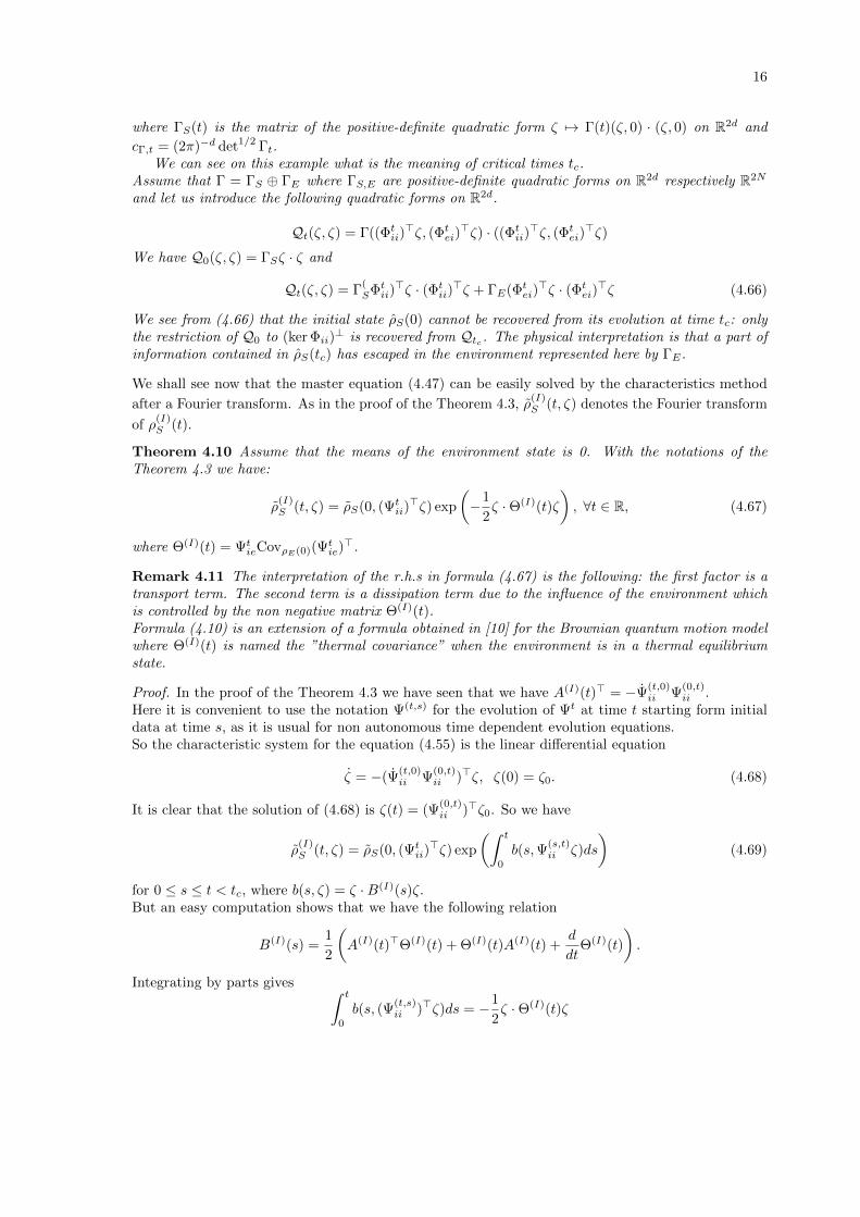
Theorem 4.10 Assume that the means of the environment state is 0. With the notations of theTheorem 4.3 we have:

ρ(I)S (t, ζ) = ρS(0, (Ψt

ii)>ζ) exp

(−1

2ζ ·Θ(I)(t)ζ

), ∀t ∈ R, (4.67)

where Θ(I)(t) = ΨtieCovρE(0)(Ψ

tie)>.

Remark 4.11 The interpretation of the r.h.s in formula (4.67) is the following: the first factor is atransport term. The second term is a dissipation term due to the influence of the environment whichis controlled by the non negative matrix Θ(I)(t).Formula (4.10) is an extension of a formula obtained in [10] for the Brownian quantum motion modelwhere Θ(I)(t) is named the ”thermal covariance” when the environment is in a thermal equilibriumstate.

Proof. In the proof of the Theorem 4.3 we have seen that we have A(I)(t)> = −Ψ(t,0)ii Ψ

(0,t)ii .

Here it is convenient to use the notation Ψ(t,s) for the evolution of Ψt at time t starting form initialdata at time s, as it is usual for non autonomous time dependent evolution equations.So the characteristic system for the equation (4.55) is the linear differential equation

ζ = −(Ψ(t,0)ii Ψ

(0,t)ii )>ζ, ζ(0) = ζ0. (4.68)

It is clear that the solution of (4.68) is ζ(t) = (Ψ(0,t)ii )>ζ0. So we have

ρ(I)S (t, ζ) = ρS(0, (Ψt

ii)>ζ) exp

(∫ t

0

b(s,Ψ(s,t)ii ζ)ds

)(4.69)

for 0 ≤ s ≤ t < tc, where b(s, ζ) = ζ ·B(I)(s)ζ.But an easy computation shows that we have the following relation

B(I)(s) =1

2

(A(I)(t)>Θ(I)(t) + Θ(I)(t)A(I)(t) +

d

dtΘ(I)(t)

).

Integrating by parts gives ∫ t

0

b(s, (Ψ(t,s)ii )>ζ)ds = −1

2ζ ·Θ(I)(t)ζ

17

and formula (4.67) follows.

It is not difficult to go back to the evolution of ρS using a change of variable and to the timeevolution of ρS(t) using inverse Fourier transform.

Corollary 4.12 Under the conditions of Theorem 4.10 we have the following formula

ρS(t, ζ) = ρS(0, (Φtii)>ζ) exp

(−1

2ζ ·Θ(t)ζ

), (4.70)

with Θ(t) = ΦtieCovρE (Φtie)>.

In particular if ρ(0) is a Gaussian state with covariance matrix ΓS(0) then ρS(t) is a Gaussian statewith the following covariance matrix ΓS(t)

ΓS(t) = ΦtiiΓS(0)(Φtii)> + ΦtieΓE(0)(Φtie)

>, ∀t ∈ R, (4.71)

where ΓE(0) = CovρE is the initial covariance of the environment.

The formula (4.70) is related with Remark 4.7 where we have computed the second moments matrix

of ρ(I)S (t).

As far as Φtii is invertible we see from (4.70) that the time evolution of ρS is reversible but this is nomore true for t ≥ tc.From formula (4.70) we get an explicit representation formula for the reduced density of the systemas a convolution integral:

Corollary 4.13 With the notations of Corollary 4.12, we have

ρ(I)S (t, z) = c

(I)S (t)

∫R2d

ρS(0,Ψ(0,t)ii z′) exp

(−1

2(z − z′) ·Θ(I)(t)−1(z − z′)

)dz′,

ρS(t, z) = cS(t)

∫R2d

ρS(0,Φ(0,t)ii z′) exp

(−1

2(z − z′) ·Θ(t)−1(z − z′)

)dz′. (4.72)

where c(I)S (t) = (2π)−d/2 det(Ψt

ii)−1 det

(Θ(I)(t)

)−1/2and

cS(t) = (2π)−d/2 det(Φtii)−1 det (Θ(t))

−1/2.

If det(Φtii) = 0 or if det((Φtie(Φtie)>) = 0, integrals in (4.72) are defined as convolutions of distribu-

tions.

Formula (4.72) shows clearly the damping influence of the environment on the system because Θ(t)is a positive matrix under our assumptions. If Θ(t) is degenerated then the Fourier transform ofexp

(− 1

2ζ ·Θ(t)ζ)

is a distribution supported in some linear subspace VS of R2d where the dampingtakes place.We can deduce an exact formula for the linear entropy S`(t) if ρS(0) is a Gaussian state.First, using the Plancherel formula we have

S`(t) = 1− (2π)−d∫R2d

(ρS(t, z))2dz

= 1− (2π)−3d

∫R2d

|ρS(t, ζ)|2dζ (4.73)

= 1− (2π)−d∫R2d

exp(−ζ ·Θ(t)ζ)|ρS(0, (Φtii)>ζ)|2dζ (4.74)

If ρS(0) is a Gaussian state we have

S`(t) = 1− det (ΓS(t))−1/2

(4.75)

where ΓS(t) is given by the formula (4.71).

18

Remark 4.14 We have seen in this section that we can compute the quantum evolution of a reducedsystem when the classical evolution of the blocks Φtii and Φtie of the total system (S)∪ (E) are known.It is hopeless to get general explicit formulas for these blocks, but this is possible in the particularcase of two oscillators (Appendix A). For a bath of N oscillators, 1 < N < +∞ the problem seemsdifficult (see Appendix B). For continuous distribution of oscillators many (non rigorous) results wereobtained concerning the Quantum Brownian Motion model (see references).

Let us close this section by giving a simple sufficient condition to get correlations between states ofthe system (S) and the environment (E). If ρ is a state of the total system (S)∪ (E) we say that (S)and (E) are uncorrelated if ρ = ρS ⊗ ρE . Note that this decomposition is unique and ρS,E = trE,S ρ.In decoherence theory [8] more difficult notions are also considered: separability and entanglement.

ρ is separable if there exists a decomposition ρ =∑j

pj ρSj ⊗ ρEj where

∑j

pj = 1, pj ≥ 0, ρSj , ρEj are

pure states respectively in HS , HE . If ρ is not separable it is said that ρ is entangled.

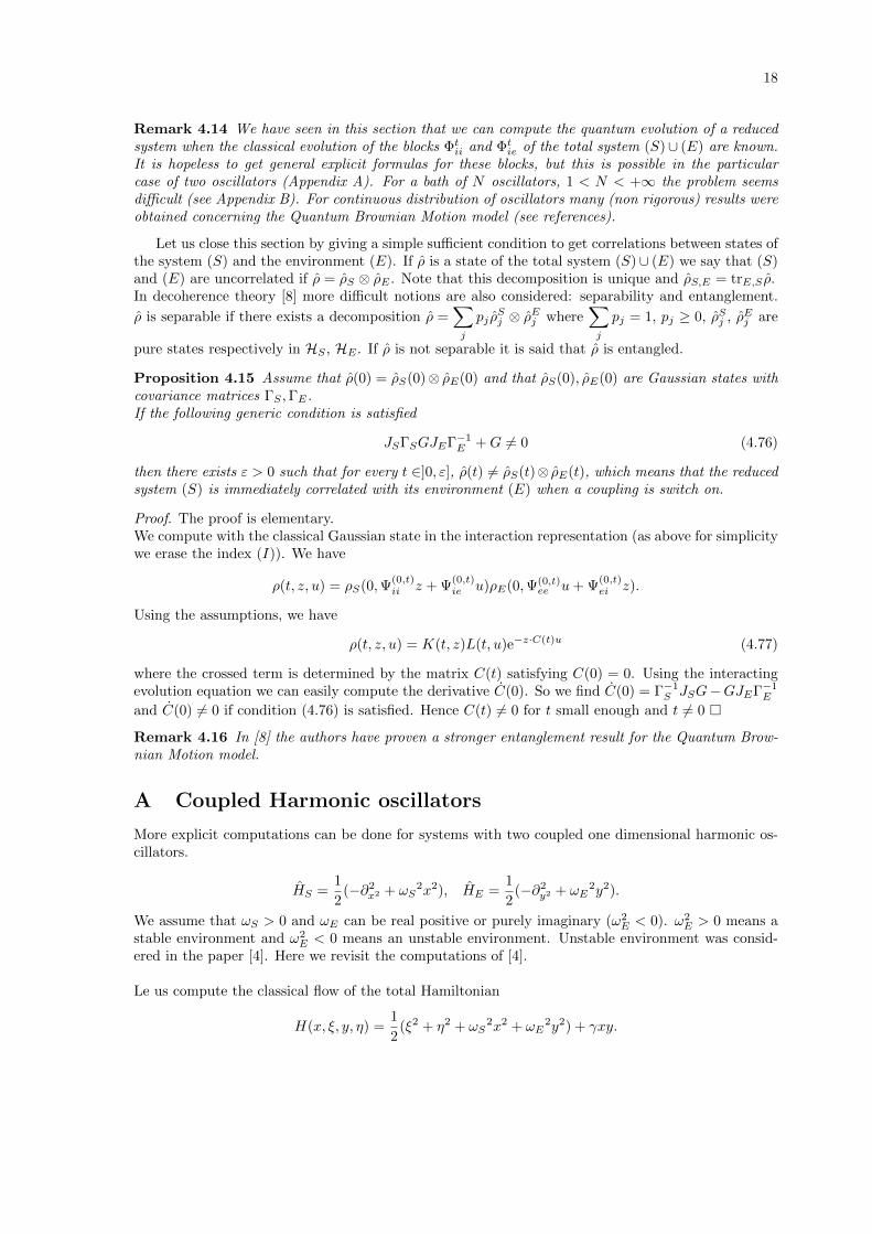
Proposition 4.15 Assume that ρ(0) = ρS(0)⊗ ρE(0) and that ρS(0), ρE(0) are Gaussian states withcovariance matrices ΓS ,ΓE.If the following generic condition is satisfied

JSΓSGJEΓ−1E +G 6= 0 (4.76)

then there exists ε > 0 such that for every t ∈]0, ε], ρ(t) 6= ρS(t)⊗ ρE(t), which means that the reducedsystem (S) is immediately correlated with its environment (E) when a coupling is switch on.

Proof. The proof is elementary.We compute with the classical Gaussian state in the interaction representation (as above for simplicitywe erase the index (I)). We have

ρ(t, z, u) = ρS(0,Ψ(0,t)ii z + Ψ

(0,t)ie u)ρE(0,Ψ(0,t)

ee u+ Ψ(0,t)ei z).

Using the assumptions, we have

ρ(t, z, u) = K(t, z)L(t, u)e−z·C(t)u (4.77)

where the crossed term is determined by the matrix C(t) satisfying C(0) = 0. Using the interactingevolution equation we can easily compute the derivative C(0). So we find C(0) = Γ−1

S JSG−GJEΓ−1E

and C(0) 6= 0 if condition (4.76) is satisfied. Hence C(t) 6= 0 for t small enough and t 6= 0

Remark 4.16 In [8] the authors have proven a stronger entanglement result for the Quantum Brow-nian Motion model.

A Coupled Harmonic oscillators

More explicit computations can be done for systems with two coupled one dimensional harmonic os-cillators.

HS =1

2(−∂2

x2 + ωS2x2), HE =

1

2(−∂2

y2 + ωE2y2).

We assume that ωS > 0 and ωE can be real positive or purely imaginary (ω2E < 0). ω2

E > 0 means astable environment and ω2

E < 0 means an unstable environment. Unstable environment was consid-ered in the paper [4]. Here we revisit the computations of [4].

Le us compute the classical flow of the total Hamiltonian

H(x, ξ, y, η) =1

2(ξ2 + η2 + ωS

2x2 + ωE2y2) + γxy.

19

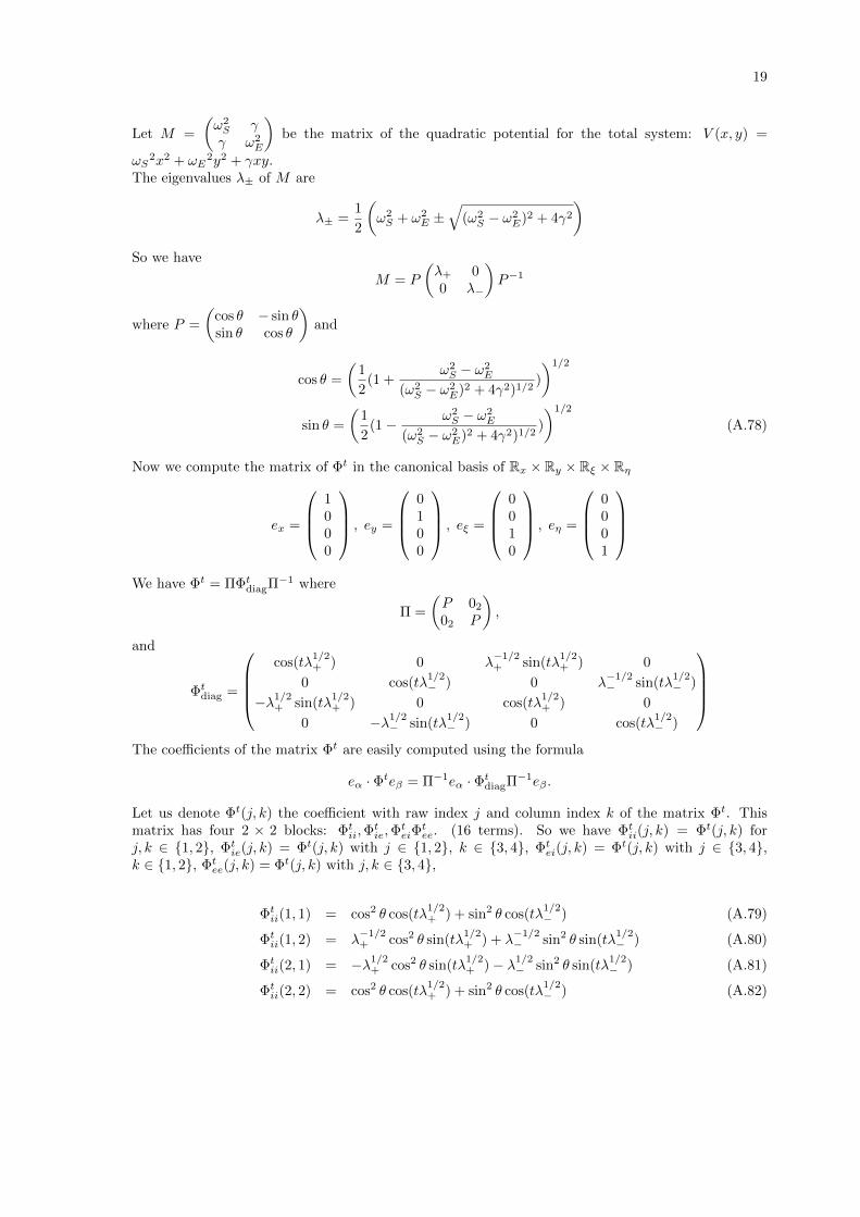
Let M =

(ω2S γγ ω2

E

)be the matrix of the quadratic potential for the total system: V (x, y) =

ωS2x2 + ωE

2y2 + γxy.The eigenvalues λ± of M are

λ± =1

2

(ω2S + ω2

E ±√

(ω2S − ω2

E)2 + 4γ2

)So we have

M = P

(λ+ 00 λ−

)P−1

where P =

(cos θ − sin θsin θ cos θ

)and

cos θ =

(1

2(1 +

ω2S − ω2

E

(ω2S − ω2

E)2 + 4γ2)1/2)

)1/2

sin θ =

(1

2(1− ω2

S − ω2E

(ω2S − ω2

E)2 + 4γ2)1/2)

)1/2

(A.78)

Now we compute the matrix of Φt in the canonical basis of Rx × Ry × Rξ × Rη

ex =

1000

, ey =

0100

, eξ =

0010

, eη =

0001

We have Φt = ΠΦtdiagΠ−1 where

Π =

(P 02

02 P

),

and

Φtdiag =

cos(tλ

1/2+ ) 0 λ

−1/2+ sin(tλ

1/2+ ) 0

0 cos(tλ1/2− ) 0 λ

−1/2− sin(tλ

1/2− )

−λ1/2+ sin(tλ

1/2+ ) 0 cos(tλ

1/2+ ) 0

0 −λ1/2− sin(tλ

1/2− ) 0 cos(tλ

1/2− )

The coefficients of the matrix Φt are easily computed using the formula

eα · Φteβ = Π−1eα · ΦtdiagΠ−1eβ .

Let us denote Φt(j, k) the coefficient with raw index j and column index k of the matrix Φt. Thismatrix has four 2 × 2 blocks: Φtii,Φ

tie,Φ

teiΦ

tee. (16 terms). So we have Φtii(j, k) = Φt(j, k) for

j, k ∈ 1, 2, Φtie(j, k) = Φt(j, k) with j ∈ 1, 2, k ∈ 3, 4, Φtei(j, k) = Φt(j, k) with j ∈ 3, 4,k ∈ 1, 2, Φtee(j, k) = Φt(j, k) with j, k ∈ 3, 4,

Φtii(1, 1) = cos2 θ cos(tλ1/2+ ) + sin2 θ cos(tλ

1/2− ) (A.79)

Φtii(1, 2) = λ−1/2+ cos2 θ sin(tλ

1/2+ ) + λ

−1/2− sin2 θ sin(tλ

1/2− ) (A.80)

Φtii(2, 1) = −λ1/2+ cos2 θ sin(tλ

1/2+ )− λ1/2

− sin2 θ sin(tλ1/2− ) (A.81)

Φtii(2, 2) = cos2 θ cos(tλ1/2+ ) + sin2 θ cos(tλ

1/2− ) (A.82)

20

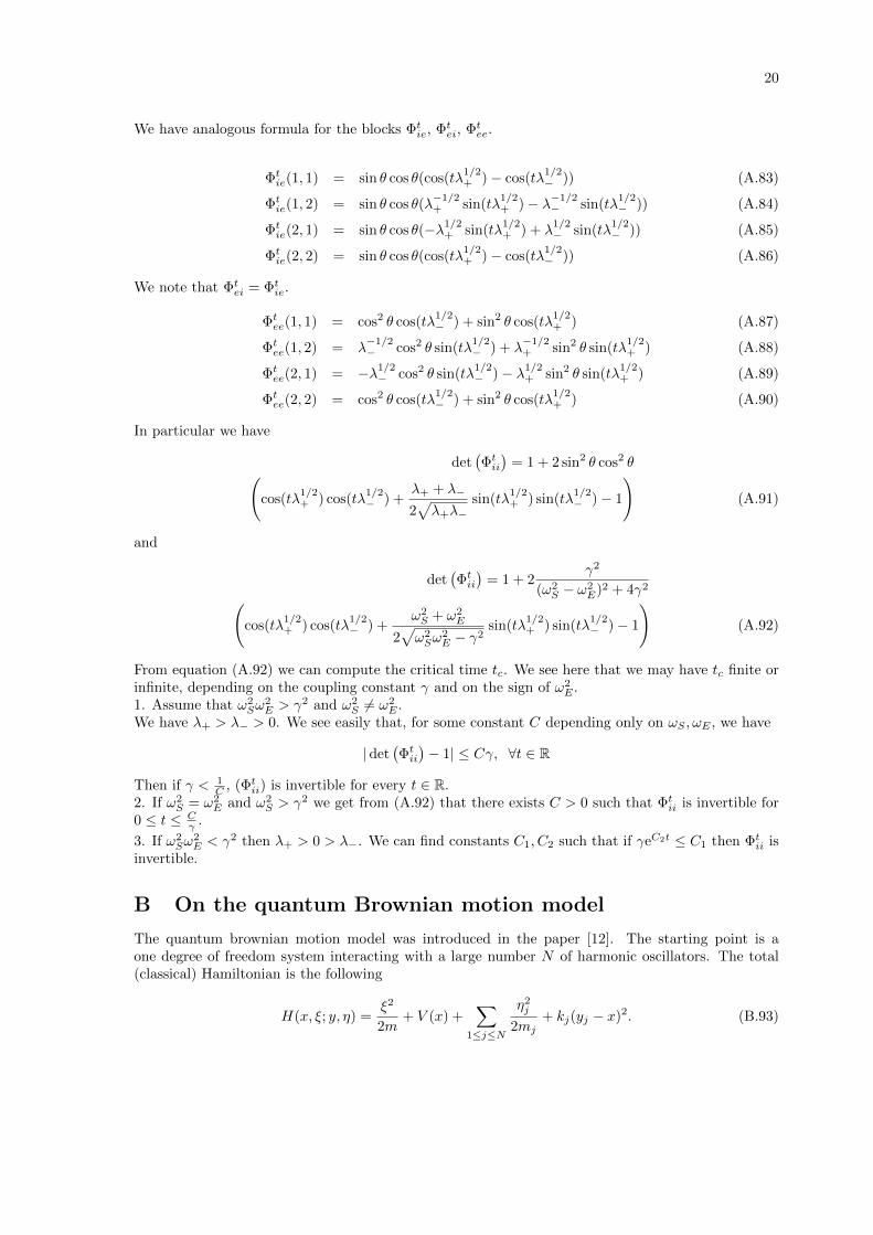
We have analogous formula for the blocks Φtie, Φtei, Φtee.

Φtie(1, 1) = sin θ cos θ(cos(tλ1/2+ )− cos(tλ

1/2− )) (A.83)

Φtie(1, 2) = sin θ cos θ(λ−1/2+ sin(tλ

1/2+ )− λ−1/2

− sin(tλ1/2− )) (A.84)

Φtie(2, 1) = sin θ cos θ(−λ1/2+ sin(tλ

1/2+ ) + λ

1/2− sin(tλ

1/2− )) (A.85)

Φtie(2, 2) = sin θ cos θ(cos(tλ1/2+ )− cos(tλ

1/2− )) (A.86)

We note that Φtei = Φtie.

Φtee(1, 1) = cos2 θ cos(tλ1/2− ) + sin2 θ cos(tλ

1/2+ ) (A.87)

Φtee(1, 2) = λ−1/2− cos2 θ sin(tλ

1/2− ) + λ

−1/2+ sin2 θ sin(tλ

1/2+ ) (A.88)

Φtee(2, 1) = −λ1/2− cos2 θ sin(tλ

1/2− )− λ1/2

+ sin2 θ sin(tλ1/2+ ) (A.89)

Φtee(2, 2) = cos2 θ cos(tλ1/2− ) + sin2 θ cos(tλ

1/2+ ) (A.90)

In particular we have

det(Φtii)

= 1 + 2 sin2 θ cos2 θ(cos(tλ

1/2+ ) cos(tλ

1/2− ) +

λ+ + λ−

2√λ+λ−

sin(tλ1/2+ ) sin(tλ

1/2− )− 1

)(A.91)

and

det(Φtii)

= 1 + 2γ2

(ω2S − ω2

E)2 + 4γ2(cos(tλ

1/2+ ) cos(tλ

1/2− ) +

ω2S + ω2

E

2√ω2Sω

2E − γ2

sin(tλ1/2+ ) sin(tλ

1/2− )− 1

)(A.92)

From equation (A.92) we can compute the critical time tc. We see here that we may have tc finite orinfinite, depending on the coupling constant γ and on the sign of ω2

E .1. Assume that ω2

Sω2E > γ2 and ω2

S 6= ω2E .

We have λ+ > λ− > 0. We see easily that, for some constant C depending only on ωS , ωE , we have

|det(Φtii)− 1| ≤ Cγ, ∀t ∈ R

Then if γ < 1C , (Φtii) is invertible for every t ∈ R.

2. If ω2S = ω2

E and ω2S > γ2 we get from (A.92) that there exists C > 0 such that Φtii is invertible for

0 ≤ t ≤ Cγ .

3. If ω2Sω

2E < γ2 then λ+ > 0 > λ−. We can find constants C1, C2 such that if γeC2t ≤ C1 then Φtii is

invertible.

B On the quantum Brownian motion model

The quantum brownian motion model was introduced in the paper [12]. The starting point is aone degree of freedom system interacting with a large number N of harmonic oscillators. The total(classical) Hamiltonian is the following

H(x, ξ; y, η) =ξ2

2m+ V (x) +

∑1≤j≤N

η2j

2mj+ kj(yj − x)2. (B.93)

21

where x, ξ are the coordinates of the system, y = (y1, · · · , yN ) and η = (η1, · · · , ηN ) are the coordinatesfor the environment. The environment consists in N harmonic oscillators and the system is connectedto each oscillator by a spring with constant kj > 0. This model is a particular case of quadratic systems

considered in section 4. if V (x) =ω2S

2 x2. The Hamiltonian can be splitted as H = HS + HE + HI

where

HS =ξ2

2m+ V (x) +

1

2(∑

1≤j≤N

kj)x2 (B.94)

HE =1

2

∑1≤j≤N

η2j

mj+ kjy

2j

(B.95)

HI = −2x(∑

1≤j≤N

kjyj) (B.96)

The classical evolution for the Hamiltonian is not explicitly given for N > 1 (we have got explicitformula in Appendix A if N = 1). It can be seen that the time evolution of the position x of thesystem satisfies the following equation [11], assuming mj = 1 for simplicity:

mx(t) +

∫ t

0

K(t− s)x(s)ds+ V ′(x(t)) +K(t)x(0) = F (t) (B.97)

where

K(t) =∑

1≤j≤N

kj cos(√kjt) (B.98)

F (t) =∑

1≤j≤N

yj(0) cos(√kjt) + ηj(0) sin(

√kjt) (B.99)

The difficulty here is that equation (B.97) is not an ODE because of the integral term.In [12, 11] the authors considered a large N limit, and a continuous distribution of oscillators, suchthat (B.97) is transformed into a stochastic differential equation where the integral term is replacedby the damping term γx(t) where γ is a damping constant (Langevin equation).

C Gaussian density matrices

We shall give here a proof of Proposition 4.2. This is consequence of a particular case of the followingWilliamson theorem (see [23] and [2] Appendix 6).

Theorem C.1 Let Γ be a positive non degenerate linear transformation in R2N . Then there exists alinear symplectic transformation S and positive real numbers λ1, · · · , λN such that

S>ΓSej = λjej , and S>ΓSej+N = λjej+N (C.100)

for 1 ≤ j ≤ N , where e1, · · · , eN , · · · , e2N is the canonical basis of R2N .

in [21] the authors gave a simple proof that we recall here. Recall the following known lemma

Lemma C.2 Let A be a non degenerate antisymmetric linear mapping in R2N . Then there exists anorthonormal basis v1, v

∗1 , · · · , vN , v∗N of R2N and positive real numbers ν1, · · · , νN, such that

Avj = νjv∗j , Av∗j = −νjvj .

22

Proof of Lemma C.2 . We proceed by induction on N . This is is obvious for N = 1.Assume N ≥ 2. Let ν1 be an eigenvalue of the symmetric matrix A2, A2v1 = ν1v1, ‖v1‖ = 1. Wecan choose a vector v∗1 and a ∈ R such that Av1 = −av∗1 and ‖v∗1‖ = 1. Then we have easily thatv1 · v∗1 = 0 and if P is the plane spanned by v1, v

∗1 then P and P⊥ are invariant by A. So we can

apply the induction assumption to A acting in P⊥ and the Lemma is proved. Proof of Theorem C.1. Consider the antisymmetric matrix A = Γ−1/2JΓ−1/2. Using Lemma C.2 wecan find an orthogonal matrix R and a diagonal matrix Ω = diagν1, ν2, · · · , νN, νj > 0, 1 ≤ j ≤ Nsuch that

R>Γ−1/2JΓ−1/2R =

(0 Ω−Ω 0

)Denote B =

(Ω−1/2 0

0 Ω−1/2

)and S = Γ−1/2RB. We get easily that S>ΓS = B2 and S>JS = J so

the proof of the Theorem C.1 follows. The N real numbers λj in Theorem C.1 are the symplectic eigenvalues of Γ. Using that S> = −JS−1Jwe see that JΓ is diagonalizable with eigenvalues ±λj , 1 ≤ j ≤ N and that λ1, · · · , λN are theeigenvalues (with multiplicities) of |JΓ| = (−JΓ2J)1/2.Proof of Proposition 4.2 We can assume assume that m = 0 and we denote ρΓ = ρΓ,0.We use the symplectic normal form for Γ given by Theorem C.1. Let R(S) be the metaplectic unitaryoperator associated with S (see for example [6]). Hence we have

R(S)∗ρΓR(S) = ρS>ΓS = ρτ1 ⊗ ρτ1 · · · ⊗ ρτN ,

where the τj are the symplectic eigenvalues of Γ−1

2 . So ρΓ is a density matrix if and only if we have0 ≤ τj ≤ 1 for 1 ≤ j ≤ d (Remark 3.4). This condition means that the symplectic eigenvalues of 2Γare greater than 1 or equivalently that 2Γ + iJ ≥ 0.We have already seen that if ρΓ is a pure state then we have 2Γ = F>F with F symplectic. Converselyif 2Γ = F>F then ρΓ is the Wigner function of a squeezed state R(F )ϕ0, ϕ0 being the standardGaussian (for details see [6]).

Gaussian states are thermal states for positive non degenerate quadratic Hamiltonians and con-versely. This can be proved as follows.Let H(u) = 1

2u · Λ where Λ is a positive non degenerate linear transformation in R2N . We considersymplectic coordinates for u: yj = u · ej and ηj = u · ej+N , 1 ≤ j ≤ N .Using Theorem C.1 we have H(u) = H∆(Su) where S is a symplectic linear transformation and

H∆(u) =∑

1≤j≤N

λju2j , uj = (xj , ξj) ∈ R2. Applying the metaplectic transformation we have H =

R(S)H∆R(S)∗ and

e−βH = R(S)e−βH∆R(S)∗

From the Melher formula for the harmonic oscillator the Weyl symbol W∆ of e−βH∆ is

W∆(y, η) =∏

1≤j≤N

exp(− tanh(βλj)(y

2j + η2

j ))

cosh(βλj)

so the Weyl symbol W of e−βH is given by

W (y, η) = W∆(S−1(y, η)).

This proves that e−βH

tre−βHis a Gaussian state. More explicit results are given in [7, 16].

References

[1] G.S. Agarwal: Entropy, the Wigner Distribution Function, and the Approach to Equilibrium ofa System of Coupled Harmonic Oscillators Phys. Rev. A 3, 828 (1971)

23

[2] V. Arnold: Mathematical Methods in Classical Mechanics Springer, Berlin-Heidelberg (1997)

[3] H.P. Breuer and F. Petruccione: The Theory of open quantum systems, Clarendon Press Oxford(2002).

[4] R. Blume-Kohout and W.H. Zurek: Decoherence form chaotic environment: an upside down”oscillator” as a model Phys. Rev. A 68, 032104 (2003).

[5] A.O. Caldeira and A.J. Leggett : Influence of damping on quantum interference: An exactlysoluble model Phys. Rev. , A31, p. 1059-1066 (1985)

[6] M. Combescure and D. Robert: Coherent states and applications in Mathematical Physics,Springer-Verlag (2012).

[7] I. Derezinski: Some remarks on Weyl pseudodifferential operators. Journees EDP, Saint Jean deMonts, expose XII, 1-14 (1993).

[8] J. Eisert and M. B. Plenio: Quantum and Classical Correlations in Quantum Brownian MotionPhys. Rev. Letters, Vol.89, No.13, 137902, p. 1-4 (2002)

[9] R. P. Feynman and F.L. Vernon: The theory of a general quantum system interacting with alinear dissipative system, Annals of physics, 24 p. 118-173 (1963).

[10] C. H. Fleming, B. L. Hu and A. Roura: Exact analytical solutions to the master equation ofBrownian motion for a general environment arXiv:1004.1603v2[quant-ph] (2010) and Ann. Phys.Vol.326, Issue 5, p.1207-1258 (2011)

[11] G.W. Ford and M. Kac: On the Quantum Langevin Equation Journal of Statistical Physics, Vol.46, Nos. 5/6, (1987)

[12] G.W. Ford, M. Kac and P.Mazur: Statistical Mechanics of Assemblies of Coupled Oscillators J.Math. Phys. 6 p.504-515 (1965)

[13] G.W. Ford and R.F. O’Connell: Exact solution of the Hu-Paz-Zhang master equation Phys. Rev.D, Vol. 64, 105020 1-13 (2001)

[14] I. Gohberg and M. G. Krein: Introduction to the theory of linear non self-adjoint operators inHilbert spaces ”Nauka” Moscow, (1965); English translation, Amer.Math. Soc.., Providence, R.I(1969)

[15] J.J. Halliwell and T. Yu: Alternative derivation of the Hu-Paz-Zhang master equation of quantumBrownian motion Phys. Rev. D 53, p.2012-2019 (1996)

[16] L. Hormander: Symplectic classification of quadratic forms, and general Mehler formulasMath. Z, 219, 413-449 (1995)

[17] B.L. Hu, J.P. Paz and Y. Zhang: Quantum Brownian motion in a general environment: Exactmaster equation with nonlocal dissipation and colored noise Phys. Rev. D 45, p.2843-2861 (1992)

[18] K. Hornberger:Introduction to Decoherence, Entangement and Decoherence Lecture Notes inPhysics, Vol. 768 p. 221-276 (2009)

[19] M.A. Nielsen and I.L. Chuang: Quantum computation and quantum information, CambridgeUniversity Press (2000).

[20] M. Schlosshauer: Decoherence and the quantum-to-classical transition, Springer-Verlag (2007).

24

[21] R. Simon, S. Chaturvedi and V. Srinivasan: Congruences and canonical forms for a positivematrix: application to Schweinler-Wigner extremum principle J. Math. Phys. 40, p.3632-3643(1999)

[22] R. Simon, E.C.G. Susarshan and N. Mukada: Gaussian Wigner distributions : a complete char-acterization Phys. Rev. A 36 p. 3868-3873, (1987)

[23] J. Williamson: On algebraic problem concerning the normal forms of linear dynamical systemsAmer. J. of Math. 58, N.1, p.141-163, (1936)

Departement de Mathematiques, Laboratoire Jean Leray, CNRS-UMR 6629Universite de Nantes, 2 rue de la Houssiniere, F-44322 NANTES Cedex 03, FranceE-mail adress: didier.robert@univ-nantes.fr