Time-optimal trajectory planning for landing onto moving platforms

Botao HuGraduate Research Assistant

Rensselaer PolytechnicInstitute

Troy, NY, USA

Sandipan MishraAssociate Professor

Rensselaer PolytechnicInstitute

Troy, NY, USA

ABSTRACTIn this paper, an algorithm for time-optimal trajectory generation is developed for landing a 6 degree-of-freedom(DOF) quadrotor onto a moving platform (with tilt, heave and pitch). The overall control architecture has a standardguidance-and-tracking control inner-outer loop structure. The outer loop (guidance control) solves the time-optimaltrajectory generation problem. Instead of directly solving the time-optimal control problem, the proposed method re-formulates this into a nonlinear programming problem that transforms the constraints on the original system dynamicsand inputs onto constraints on the system states. This transformation is based on the differential flatness propertyof the quadrotor dynamics. The proposed method is computationally efficient and can also incorporate the collisionavoidance constraints. We further demonstrate that this time-optimal problem can be resolved at periodic intervals (ifdisturbances and unmodeled dynamics deviate the quadrotor from the optimal trajectory). For the inner loop, a tra-jectory tracking controller is also designed that can deal with system uncertainties and external disturbances that mayaffect the quadrotor’s dynamics. Simulation and experimental results show the effectiveness of the proposed method.

INTRODUCTION

There has been growing interest in Vertical Taking Off andLanding (VTOL) autonomous aerial vehicles (AAVs) for a va-riety of applications, including aerial imaging, surveillance,and law enforcement. One important capability for suchAAVs is autonomous landing onto either a stationary or mov-ing platform (Refs. 1–4). However, autonomous landing ontoa platform (such as a ship deck on sea or a moving target) isoften difficult because of the stringent constraints on safety,collision avoidance, soft contact requirements, and limitedlanding time. Therefore, a proper landing trajectory that mini-mizes the total time-to-land and satisfies the safety constraintsshould be generated in real-time prior to executing such a ma-neuver.

In our earlier work, (Refs. 5,6), we demonstrated the design ofsuch time-optimal landing paths when the platform was hor-izontal and only translated in the vertical direction. (Ref. 7)presented an algorithm for time-optimal trajectory design thatexploited decoupled dynamics in the x and z directions. How-ever, if the platform is tilting in addition to movement in thehorizontal and vertical directions, the trajectory generationproblem is more challenging because the horizontal and ver-tical dynamics are coupled and thus the decoupled trajectorygeneration approach (as in (Ref. 7)) is not applicable.

In this paper, we address the more general trajectory gen-

Presented at the AHS International 73rd Annual Forum &Technology Display, Fort Worth, Texas, USA, May 9–11, 2017.Copyright c© 2017 by AHS International, Inc. All rights reserved.

x position (m)

-3 -2 -1 0 1 2 3

z po

sitio

n (m

)

0

1

2

3

4

5

Time optimal maneuver

moving

fixed

Tim

e (s

)

0

0.2

0.4

0.6

0.8

1

1.2

Fig. 1: Trajectories for time-optimal landing onto stationaryand moving platforms. The trajectory on the left illustrateslanding onto a fixed platform. The trajectory on the right il-lustrates landing onto an oscillating and tilting platform. Thegreen bar represents the platform position.

eration problem to generate a time-optimal trajectory for a6-DOF quadrotor landing onto a 3-DOF platform (with theheave, pitch and roll, which are selected because they are typ-ically more important than the lateral motion and the yaw mo-tion).

In general, an optimal control problem must be solved to ob-tain the time-optimal landing trajectory. One approach to-wards this goal is to directly solve the optimal control prob-lem. This approach, as demonstrated in (Refs. 8, 9), is time-

1

consuming because the quadrotor dynamics are nonlinear andfurthermore it is difficult to incorporate collision avoidanceconstraints into the optimal control problem. Another ap-proach using model predictive control was proposed by Ngo(Ref. 3). The authors demonstrated the performance of the al-gorithm through simulation of a full-scale helicopter modellanding onto a ship deck. The algorithm used a surrogatecost to penalize the time-to-land, instead of directly penal-izing time-to-land. The time-optimality of the algorithm wasthus not verifiable.

In contrast, (Ref. 10) used the differential flatness propertyof the quadrotor dynamics to transform the original optimalcontrol problem into a nonlinear programming problem andgenerate a point-to-point time-optimal maneuver trajectory.This trajectory generation method was shown to be compu-tationally efficient and could incorporate the obstacle avoid-ance constraints. This approach provides an elegant mecha-nism for transforming the constraints on the system input anddynamics onto the system states, which ultimately decreasesthe computational complexity of the problem through suitableparameterization. However, this algorithm did not accountfor time-varying platform motion as a terminal state constraintand thus is not directly applicable for landing onto a movingplatform.

However, inspired by (Ref. 10), this paper develops a time-optimal landing trajectory generation method for a 6-DOFquadrotor landing onto a heaving, rolling and pitching plat-form. The general idea behind the proposed method is to for-mulate a nonlinear programming problem that uses the systemstates as the optimization variables (instead of the input) usingdifferential flatness. The advantages of the proposed the tra-jectory generation method are that it can directly incorporatethe time-varying motion of the platform and collision avoid-ance constraints during the landing maneuver. This paper isan extension of the method presented in our recent submis-sion (Ref. 11), where a simplified quadrotor model (3-DOF)was used to generate a time-optimal landing trajectory (Fig.1 shows the time-optimal trajectories for landing onto a sta-tionary platform and a heaving and pitching 2-DOF platformbased on method presented in (Ref. 11)). We further demon-strate that the proposed method can be used in real-time (anditeratively be solved at each time-step in a model predictivemanner since the computation times are sufficiently small).

We first present the 6-DOF quadrotor dynamics model andformulate the time-optimal trajectory generation problem. Wethen describe a mechanism to reformulate this problem usingdifferential flatness into a computationally efficient structure.A tracking (inner loop) controller is then proposed for track-ing this time-optimal trajectory. Simulation and experimentalresults are then presented to validate the proposed algorithms.Finally, we conclude with challenges, future directions, andextensions for this work.

Fig. 2: Schematic of the quadrotor and the platform prior tolanding. The quadrotor has six degrees of freedom and theplatform has three degrees of freedom.

DYNAMICAL MODEL AND PROBLEMFORMULATION

In this section, we first present the 6-DOF system dynamicsmodel for a quadrotor and then formulate the time-optimallanding problem as a constrained optimization problem.

6-DOF Quadrotor model

We model the quadrotor as a 6-DOF rigid body, as shown inFig. 2. Denote the inertial frame as I, the body frame as B; andthe system state as xxx = (pppT , pppT ,θθθ T ,ΩΩΩT )T , where the vectorppp= (x,y,z)T is the position and ppp= (x, y, z)T is the velocity ofthe quadrotor in the inertial frame. The vector θθθ = (α,β ,γ)T

contains the roll, pitch and yaw Euler angles. The vector ΩΩΩ =(p,q,r)T is the angular velocity about the body frame bases.The system input is denoted as uuu = (T,τx,τy,τz)

T where T isthe thrust and τx,τy,τz are the torques around the body framebases. The dynamics of the system can be described by:

mppp = R(α,β ,γ)

00T

− 0

0mg

IΩΩΩ =−ΩΩΩ× IΩΩΩ+

τxτyτz

, (1)

where m is the mass of the quadrotor, g is the gravitationalacceleration and I is the inertia matrix. R(α,β ,γ), the rotationmatrix corresponding to the body frame B with respect to theinertial frame I, is a function of the Euler angles. The rotationis described on a Z-Y-X ordering. The operator ‘×’ denotesthe cross product. The angular velocity ΩΩΩ = (p,q,r)T can berepresented as a function of the first order derivatives of theEuler angles θθθ = (α, β , γ)T . The rotation matrix R and theangular velocity ΩΩΩ can be represented as:

R =

cβcγ cγsαsβ − cαsγ sαsγ + cαcγsβ

cβ sγ cαcγ + sαsβ sγ cαsβ sγ− cγsα

−sβ cβ sα cαcβ

ΩΩΩ =

1 0 −sβ

0 cα cβ sα

0 −sα cαcβ

θθθ .

(2)

2

quadrotordynamics

platformmotion

xd

platformstate

x∗

desiredstate

desiredinput

u∗

feedback

feedforwardcontrol

controltrajectorygeneration

mapping

uinput

p

p

θΩ

xquadrotorstate

guidancecontrol

trackingcontrol

control structure

x∗

Fig. 3: Schematic of the proposed control architecture. The control architecture consists of two modules in the dashed box. Theguidance control module outputs the reference trajectory and the tracking control module generates the thrust command for thequadrotor.

‘c’ and ‘s’ are shorthand forms of cosine and sine functions.All the Euler angles are constrained to a feasible set. Theconstraints on the Euler angles can be represented as:αmin

βminγmin

≤ θθθ ≤

αmaxβmaxγmax

. (3)

Control architecture

Fig. 3 shows the cascade two-loop structure of the proposedalgorithm. The outer loop is the guidance control where thetime-optimal landing trajectory xxx∗ is first generated based onthe platform state xxxd and the quadrotor state xxx. Then the gen-erated optimal reference trajectory is used to obtain a refer-ence input uuu∗. The inner loop is a standard Model ReferenceAdaptive Controller (MRAC) (Ref. 12), which takes in thereference trajectory xxx∗ and the state of the quadrotor xxx andgenerates a control command uuu that achieves robust trajectorytracking performance.

Problem formulation

We first focus on the design of the trajectory generation block(outer loop). The objective of this trajectory generation blockis to create an optimal trajectory for the quadrotor to landonto a translating and tilting platform (with a known but time-dependent trajectory) within the smallest possible time, t f .

Denote xxxd(·) = (pppTd , pppT

d ,θθθTd ,ΩΩΩ

Td )

T ∈ ℜ12 as the state of theplatform. pppd = (xd ,yd ,zd)

T is the platform position, θθθ d =(αd ,βd ,γd)

T as the Euler angles of the platform and ΩΩΩd =(pd ,qd ,rd)

T as the angular velocity of the platform. Let t f bethe final (as yet unknown) time, xxx0 as the initial state for thequadrotor. Denote xxxd(t f ) as the state of the platform at thefinal time. The time-optimal quadrotor landing problem canbe formulated as an optimal control problem as (4):

argminuuu(t),t f

J = t f

s.t xxx = f (xxx,uuu), xxx ∈ℜ6

xxx(t = 0) = xxx0xxx(t = t f ) = xxxd(t f ) ∈ℜ6

ggg(xxx(t)) ∈ GGG, ∀t ∈ [0, t f ]uuumin ≤ uuu(t)≤ uuumax, ∀t ∈ [0, t f ]

(4)

ggg(xxx) captures the (safety and feasibility) constraints includingthe Euler angle limits, obstacle avoidance constraints and thecollision avoidance constraints. The exact definitions of theconstraints will be introduced in the following section.

The problem described above is a standard time-optimal con-trol formulation. Direct solution of this problem is typicallytime-consuming, as was pointed out in (Ref. 7). Therefore, wereformulate the problem into a nonlinear programming prob-lem that is computationally tractable for real-time implemen-tation, as follows.

TIME-OPTIMAL TRAJECTORYGENERATION ALGORITHM

In this section, we describe the time-optimal trajectory gener-ation algorithm and a force/torque mapping scheme that gen-erates the ideal (feedforward) input, based on the differentialflatness property of the quadrotor dynamics.

Differentially flat systems

We briefly recall the differential flatness property of a dynam-ical system. A detailed explanation of differentially flat sys-tems can be found in (Ref. 13).

Definition: Given a system xxx = f (xxx,uuu), a flat output yyy is de-fined as a function of the derivatives of the state and systeminput:

yyy = φ(xxx,uuu, uuu, · · · ,uuu(i)). (5)

The system is called differentially flat if the system state andsystem input can be represented by the derivatives of the sys-tem flat output, i.e.,

xxx = φx(yyy, yyy, yyy, · · · ,yyy( j))

uuu = φu(yyy, yyy, yyy, · · · ,yyy( j−1)).(6)

It is straightforward to show that the dynamics for this 6-DOFquadrotor model represented in (1) is indeed differentiallyflat (Ref. 14) . Choosing the flat output as yyy = (pppT ,ΩΩΩT )T ,the input for this system can be represented as a function ofderivatives of the flat output as shown below.

3

Denote xxxa as the augmented system state and it is defined as:

xxxa = (pppT , pppT ,θθθ T , θθθT, pppT ,ΩΩΩT ,ΩΩΩ

T)T (7)

xxxa is a vector of flat output and derivatives. The inputs for thesystem can be represented by function ψ1(xxx) and ψ2(xxx) as:0

0T

= ψ1(xxxa) = R−1(mppp+

00

mg

)τxτyτz

= ψ2(xxxa) = IΩΩΩ+ΩΩΩ× IΩΩΩ

. (8)

The inputs, namely ψ1(xxxa), ψ2(xxxa) are constrained to theirfeasible ranges respectively. The constraints on the input uuucan thus be represented as : 0

0Tmin

≤ ψ1(xxxa)≤

00

Tmax

τxminτyminτzmin

≤ ψ2(xxxa)≤

τxmaxτymaxτzmax

. (9)

Remark: The key benefit of using the differentially flat prop-erty is that we can avoid the integration of the nonlinear dy-namics, as mentioned in (Ref. 10).

Trajectory generation

Based on the new constraints (9) extracted above, we nowdescribe time-optimal trajectory generation algorithm. Theidea is to reformulate the original optimal control problem de-scribed in (4) into a nonlinear programming problem that ismore amenable to numerical solution in real time on-the-fly.

Cost function For time-optimallanding, the objective func-tion to be minimized is the total time to land. The cost func-tion is thus defined same as defined in (4) as: min J = t f .

Optimization variables Although the original system dy-namics (1) for optimization are continuous, for numericaltractability, the system dynamics are discretized into N seg-ments. The number of segments, N, is chosen and fixed apriori. A proper selection of N is the result of the trade-off be-tween the accuracy and the computational time necessary forthe numerical solution of the problem. In the RESULTS sec-tion of this paper, a simulation result that shows the trade-offbetween the accuracy and the computational time is presentedand a proper number of segments are selected. The samplingtime ts for each segment can be calculated from the total time:

ts =t f

N−1(10)

The discretized state variable Xk represents the state variablesat k-th sampling time. The elements in Xk are:

Xk = (pppTk , pppT

k , pppTk ,θθθ

Tk , θθθ

Tk ,ΩΩΩ

Tk ,ΩΩΩ

Tk )

T ∈ℜ21 (11)

Optimization constraints The constraints in general may beclassified into two categories, namely, the discretized kine-matics constraints and system-level constraints. The latter setof constraints may vary for different cases and typically in-clude collision avoidance, actuator limits, state bounds, etc.Here, we present formulations of typical constraints.

1. Discretized kinematics constraints: based on the systemdiscretization, the discretized state variable X(k) mustsatisfy the following constraints:

pppk+1pppk+1θθθ k+1ΩΩΩk+1

−

pppk + pppkts + pppkt2s2

pppk + pppktsθθθ k + θθθ ktsΩΩΩk + ΩΩΩkts

=

0003000300030003

∀k = 1,2, · · · ,N−1

(12)

2. System input constraints: based on (9), the constraints onuuu can be expressed as constraints on the system states: 0

0Tmin

≤ ψ1(Xk)≤

00

Tmax

τxminτyminτzmin

≤ ψ2(Xk)≤

τxmaxτymaxτzmax

∀k = 1,2, · · · ,N

(13)

3. Initial and final state constraints: the initial state and thefinal state of the quadrotor must match the given initialstate xxx0 and the platform final state xxxd(t f ) respectively.The constraints that enforce these are:[

pppT1 pppT

1 θθθT1 θθθ

T1 ΩΩΩ

T1

]T− xxx0 = 00015[

pppTN pppT

N θθθTN θθθ

TN ΩΩΩ

TN

]T− xxxd(t f ) = 00015

(14)It should be noted that the platform final state xxxd(t f ) canbe time varying if the platform motion can be explicitlyexpressed as a function of total time t f .

4. Bounds on the state variables: some elements of the op-timization variable Xk may be bounded to enforce statebounds or input limits, etc. These bounds on Xk are typ-ically linear constraints. Examples include (1) the totaltime t f is positive, (2) the Euler angles should be smallenough to justify the small angle assumption from (3) forall k = 1,2, · · · ,N. These constraints are written as

0≤ t f ,αminβminγmin

≤ θθθ k ≤

αmaxβmaxγmax

,∀k = 1,2, · · · ,N

(15)

Formulation of the optimization problem With the defini-tion of the optimization variables, constraints and cost func-tions, a new formulation of the optimization problem (4) may

4

now be constructed. By stacking the constraints describedpreviously and denote the constraint function as g(Xk), theoptimization problem (4) can now be written as

argminXk,t f

J = t f

s.t gmin ≤ g(Xk, t f )≤ gmax,∀k = 1,2, · · · ,N.(16)

Remark: The optimization problem can then be modeled (us-ing CasADi (Ref. 15)) and solved (with Ipopt (Ref. 16)) usingstandard NLP solvers.

Choice of initial guess for optimization In the previoussubsection, a nonlinear programming problem was formu-lated. Usually an accurate initial feasible guess is necessaryto solve such a (typically nonconvex) nonlinear programmingproblem. Here, we have used a randomized approach to gen-erate a set of initial guesses.

Generating the reference trajectory The solution of theoptimization problem above generates the optimal state tra-jectory, XXX∗ =

[X∗1 X∗2 · · · X∗k · · · X∗N

]∈ ℜ21N , which is

the state variable at each sampling time. For the k−th sample,the optimal solution is X∗k

X∗k =[

ppp∗tk ppp∗Tk ppp∗Tk θθθ∗Tk θθθ

∗Tk ΩΩΩ

∗Tk ΩΩΩ

∗Tk

]k = 1,2, · · · ,N

(17)

X∗k contains the optimal reference state trajectory xxx∗. The ref-erence state at k−th sampling time is denoted as

xxx∗ =[ppp∗Tk ppp∗Tk θθθ

∗Tk ΩΩΩ

∗Tk]∈ℜ

12 (18)

Generating the optimal input (force/torque) In the previ-ous subsection, the state reference trajectory was generatedbased on the solution of the optimization problem XXX∗. Basedon the differential flatness property of the quadrotor dynam-ics, the ideal reference input uuu∗ can then be obtained. Themapping from the state to the force and torque input is givenby (8). By replacing the state with the solution from the pre-vious subsection, the optimal input uuu∗ can be calculated:

T ∗ =[0 0 1

]ψ1(xxxX∗k

)τ∗xτ∗yτ∗z

= ψ2(xxxX∗k)

uuu∗ =[T ∗ τ∗x τ∗y τ∗z

]T(19)

It should be noted that uuu∗ is the ideal input. If there are ex-ternal disturbances or system uncertainties, directly applyingthe ideal input uuu∗ without any feedback stabilization or distur-bance rejection will not guarantee good tracking performance.

TRACKING CONTROL (INNER LOOP)DESIGN

Thus far we have generated a suitable time-optimal referencetrajectory xxx∗ and the corresponding input uuu∗. In this section,a tracking control algorithm is described that generates thecontrol input uuu based on the reference input to track the ref-erence trajectory. The proposed trajectory tracking controllerconsists of a feedback and a feedforward controller, describedbelow.

Feedback controller design The feedback controller is astandard linear quadratic regulator (LQR). It is based on lin-earized system dynamics, as in (Ref. 17). The linear dynamicscan be written as

xxx = Axxx+BuuuA ∈ℜ12×12,B ∈ℜ12×4 (20)

The feedback controller is of the form

u f b = K(xxx∗− xxx), (21)

where K is obtained from a standard LQR design. The refer-ence state is as obtained in the previous section.

Feedforward controller design A model reference adaptivecontroller (MRAC) similar to (Ref. 12) is used as the feedfor-ward inner loop controller, to account for uncertainty in thesystem model. The control law is

u f f = δδδηηη = Kxxxx+Kruuu∗

δδδ =[Kx Kr

],η =

[xxxuuu∗

]Kx ∈ℜ4×12,Kr ∈ℜ4×4

(22)

The matrix δδδ is a matrix of time-varying adaptive parameters.The vector ηηη is the vector of system state xxx and system refer-ence input uuu∗. The classical adaptive law is given by

Kx = ΓxBT PexxxT

Kr = ΓrBT Peuuu∗T (23)

where Γx and Γr are diagonal, positive definite matrices ofadaptive gains, e = xxx∗− xxx is the model tracking error. P isthe positive definite solution of the Lyapunov equation AT P+PA =−Q where Q any positive definite matrix of compatibledimension.

RESULTS

Experimental setup

We now briefly describe the experimental setup shown in Fig.4. The set up consists of a central computer, a quadrotor,a platform and a motion capture system. A Hummingbirdquadrotor from the Ascending Technology is used for the ex-perimental validation. The platform has heave, roll, and pitchdegrees of freedom. The heave motion is generated by a step

5

quadrotor

platform

xd

x∗

u∗ trackingcontrol

guidancecontrol

u

p

p

θΩ

x

computer

motioncapture

x, xd

Fig. 4: Schematic of the setup for quadrotor landing exper-iments. In this setup, the computer sends the control com-mands to the quadrotor. The position and orientation of thequadrotor and the platform are captured by the motion cap-ture system and fed back to the computer at 100 Hz.

Number of segmentations0 50 100 150 200

com

puta

tiona

l tim

e (s

)

0

1

2

3

4

5Trade off between computational time and accuracy

time

time-to-land

time-

to-la

nd (

s)

0.74

0.75

0.76

0.77

0.78

0.79

Fig. 5: Plot of trade-off between the accuracy and the totaltime as the number of segments N is increased. The dashedline shows the computational time required to solve the time-optimal problem and the solid time shows the total time-to-land. The total time-to-land converges to an optimal (min-imum) value, and the computational time increases signifi-cantly if N is larger than 185.

motor and the roll/pitch motion are generated using two servomotors. Several infrared markers are attached to the quadrotorand the platform. The position and orientation of these mark-ers are captured by the motion capture system and sent to thecomputer. The trajectory generation algorithm and the track-ing control algorithm are implemented on MATLAB on thisLinux computer. The generated control commands are thensent wirelessly to the quadrotor at 100Hz update rate.

For simulation results, we use the quadrotor model parameterspresented in (Ref. 18). The feasible system input set is definedas follows:

1 N ≤ T ≤ 30 N−8 Nm≤ τx ≤ 8 Nm−8 Nm≤ τy ≤ 8 Nm−8 Nm≤ τz ≤ 8 Nm

(24)

The roll, pitch and yaw Euler angles are all bounded within[−π

2 ,π

2 ] rad.

Choice of number of segments N

In this subsection, we first perform a series of simulations tochoose the best number of segments N for the trajectory gen-eration algorithm. Figure 5 shows the computation time andfinal time for various choices of the number of segments N.The initial position of the quadrotor was (0 m,0 m,2 m). Thefinal state xxxd(t f ) is defined as

pppd(t f ) = (1 m,1 m,sin(t f ) m)pppd(t f ) = (0 m/s,0 m/s,cos(t f ) m/s)θθθ d(t f ) = (−0.6sin(t f ) rad,0.6sin(t f ) rad,0 rad).

(25)

With a larger N, the computational time (blue dashed line) in-creases, while the optimal total time-to-land (brown solid line)reduces and converges to a minimum value, which is the trueoptimal time-to-land. It is interesting to note that the compu-tational time increases significantly after N > 185 except forsome outliers. Therefore, we use N = 185 as the ideal seg-ment number in the following simulations. Furthermore, wenote that for N = 185, the optimization problem can be solvedin less than 1 second, therefore opening up the possibility forreal-time implementation.

Simulation of time-optimal landing onto a heaving-rolling-pitching platform

In this simulation, a time-optimal trajectory is designed for aquadrotor landing onto a heaving, rolling and pitching plat-form. The quadrotor initial position is (0 m,0 m,2 m). Theplatform motion xxx(t f ) is defined as:

pppd(t f ) = (1 m,1 m,sin(t f ) m)pppd(t f ) = (0 m/s,0 m/s,cos(t f ) m/s)θθθ d(t f ) = (−0.6sin(t f ) rad,0.6sin(t f ) rad,0 rad).

(26)

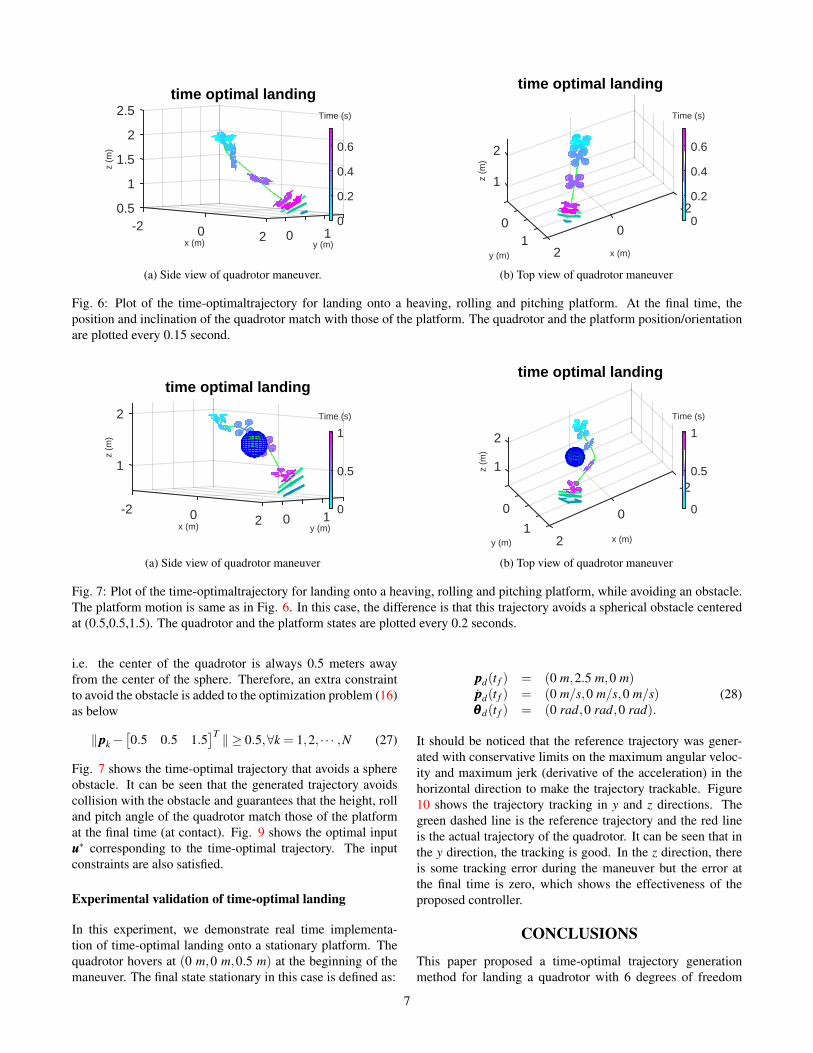
Fig. 6 illustrates a plot of the time-optimal landing maneuver,(a) is the side view while (b) shows the top view. It can be seenfrom both the side view and the top view figures that at thefinal time instant of the maneuver, the quadrotor lands on theplatform with the height, roll angle and pitch angle matchingthat of the platform. The total time for the maneuver is 0.75seconds. Fig. 8 shows the corresponding optimal input for thislanding maneuver. It can be seen that the inputs are within thefeasible bounds defined in (24).

Simulation of time-optimal landing with collision avoid-ance

In this simulation, in addition to landing onto a platform withsame motion defined in (28), there is a spherical obstacle cen-tered at (0.5 m,0.5 m,1.5 m) with a radius of 0.25 meter. Weassume that a safety distance from the center of the quadrotorto the surface of the sphere of 0.25 meter must be maintained,

6

y (m)1

time optimal landing

020x (m)

-2

2.5

0.5

1

1.5

2

z (m

)Time (s)

0

0.2

0.4

0.6

(a) Side view of quadrotor maneuver.

-2

time optimal landing

x (m)

0

21

y (m)

0

2

1z (m

)

Time (s)

0

0.2

0.4

0.6

(b) Top view of quadrotor maneuver

Fig. 6: Plot of the time-optimaltrajectory for landing onto a heaving, rolling and pitching platform. At the final time, theposition and inclination of the quadrotor match with those of the platform. The quadrotor and the platform position/orientationare plotted every 0.15 second.

1y (m)

time optimal landing

02x (m)0-2

2

1

z (m

)

Time (s)

0

0.5

1

(a) Side view of quadrotor maneuver

-2

time optimal landing

x (m)

0

21

y (m)

0

1

2

z (m

)

Time (s)

0

0.5

1

(b) Top view of quadrotor maneuver

Fig. 7: Plot of the time-optimaltrajectory for landing onto a heaving, rolling and pitching platform, while avoiding an obstacle.The platform motion is same as in Fig. 6. In this case, the difference is that this trajectory avoids a spherical obstacle centeredat (0.5,0.5,1.5). The quadrotor and the platform states are plotted every 0.2 seconds.

i.e. the center of the quadrotor is always 0.5 meters awayfrom the center of the sphere. Therefore, an extra constraintto avoid the obstacle is added to the optimization problem (16)as below

‖pppk−[0.5 0.5 1.5

]T ‖ ≥ 0.5,∀k = 1,2, · · · ,N (27)

Fig. 7 shows the time-optimal trajectory that avoids a sphereobstacle. It can be seen that the generated trajectory avoidscollision with the obstacle and guarantees that the height, rolland pitch angle of the quadrotor match those of the platformat the final time (at contact). Fig. 9 shows the optimal inputuuu∗ corresponding to the time-optimal trajectory. The inputconstraints are also satisfied.

Experimental validation of time-optimal landing

In this experiment, we demonstrate real time implementa-tion of time-optimal landing onto a stationary platform. Thequadrotor hovers at (0 m,0 m,0.5 m) at the beginning of themaneuver. The final state stationary in this case is defined as:

pppd(t f ) = (0 m,2.5 m,0 m)pppd(t f ) = (0 m/s,0 m/s,0 m/s)θθθ d(t f ) = (0 rad,0 rad,0 rad).

(28)

It should be noticed that the reference trajectory was gener-ated with conservative limits on the maximum angular veloc-ity and maximum jerk (derivative of the acceleration) in thehorizontal direction to make the trajectory trackable. Figure10 shows the trajectory tracking in y and z directions. Thegreen dashed line is the reference trajectory and the red lineis the actual trajectory of the quadrotor. It can be seen that inthe y direction, the tracking is good. In the z direction, thereis some tracking error during the maneuver but the error atthe final time is zero, which shows the effectiveness of theproposed controller.

CONCLUSIONS

This paper proposed a time-optimal trajectory generationmethod for landing a quadrotor with 6 degrees of freedom

7

time (s)0 0.2 0.4 0.6

thru

st (

N)

0

20

40input thrust

time (s)0 0.2 0.4 0.6to

rque

(m

/s)

-10

0

10torque 1

time (s)0 0.2 0.4 0.6to

rque

(m

/s)

-10

0

10torque 2

time (s)0 0.2 0.4 0.6

torq

ue (

m/s

)

-10

0

10torque 3

Fig. 8: Plot of input for the time-optimal trajectory shownin Fig. 6. All the inputs satisfy the constraints for feasi-bility.

time (s)0 0.2 0.4 0.6 0.8

thru

st (

N)

0

20

40input thrust

time (s)0 0.2 0.4 0.6 0.8to

rque

(m

/s)

-10

0

10torque 1

time (s)0 0.2 0.4 0.6 0.8to

rque

(m

/s)

-10

0

10torque 2

time (s)0 0.2 0.4 0.6 0.8

torq

ue (

m/s

)-10

0

10torque 3

Fig. 9: Plot of input for the time-optimaltrajectory shownin Fig. 7. All the inputs satisfy the constraints for feasi-bility.

time (s)

0 0.5 1 1.5 2 2.5

y po

sitio

n (m

)

0

0.5

1

1.5

2

2.5

3y tracking

actualreference

(a) y direction tracking

time (s)

0 0.5 1 1.5 2 2.5

z po

sitio

n (m

)

0

0.2

0.4

0.6

0.8

1z tracking

actualreference

(b) z direction tracking

Fig. 10: Plot of the quadrotor trajectory landing onto a stationary ground. The dashed line is the reference trajectory and thered line is the actual tracking trajectory.

8

onto a heaving, rolling and pitching platform. The time-optimal control problem is transformed into a nonlinear pro-gramming problem by applying the differential flatness prop-erty of the quadrotor dynamics, which improves the compu-tational tractability. A trajectory tracking controller based onthe Model Reference Adaptive Control is designed to trackthe reference trajectory in a real experiment. Simulation andexperimental results show the effectiveness of the proposedtrajectory generation method. We demonstrate real-time im-plementation of the system

Author contact: Botao Hu hub2@rpi.edu; Sandipan Mishramishrs2@rpi.edu.

ACKNOWLEDGMENT

This work was funded by Office of Naval Research underaward N00014-16-1-2705.

REFERENCES1Sanchez-Lopez, J. L., Saripalli, S., and Campoy, P., “Au-

tonomous ship board landing of a VTOL UAV,” American He-licopter Society 69th Forum, 2013.

2Horn, J. F., Tritschler, J., and He, C., “Autonomous ControlModes and Optimized Path Guidance for Shipboard Landingin High Sea States,” Technical report, DTIC Document, 2014.

3Ngo, T. D., Constrained control for helicopter shipboardoperations and moored ocean current turbine flight control,Ph.D. thesis, Dept of Aerospace Eng., Virginia PolytechnicInst, Blacksburg, VA, 2016.

4Holmes, W. and Langelaan, J., “Autonomous ship-boardlanding using monocular vision,” 72nd American HelicopterSociety Forum, May 17 2016.

5Hu, B., Lu, L., and Mishra, S., “Fast, safe and precise land-ing of a quadrotor on an oscillating platform,” American Con-trol Conference, 2015., July 2015.

6Hu, B., Lu, L., and Mishra, S., “A control architecture forfast and precise autonomous landing of a VTOL UAV onto anoscillating platform,” AHS 71st Auunal Forum, May 2015.

7Hehn, M. and DAndrea, R., “Real-time trajectory gen-eration for quadrocopters,” IEEE Transactions on Robotics,Vol. 31, (4), 2015, pp. 877–892.

8Hehn, M., Ritz, R., and DAndrea, R., “Performance bench-marking of quadrotor systems using time-optimal control,”Autonomous Robots, Vol. 33, (1-2), 2012, pp. 69–88.

9Lai, L.-C., Yang, C.-C., and Wu, C.-J., “Time-OptimalControl of a Hovering Quad-Rotor Helicopter,” Journal of In-telligent and Robotic Systems, Vol. 45, (2), 2006, pp. 115–135.

10Van Loock, W., Pipeleers, G., and Swevers, J., “Time-optimal quadrotor flight,” Proc. of the 2013 European ControlConference (ECC), 2013.

11Hu, B. and Mishra, S., “A time-optimal trajectory genera-tion algorithm for quadrotor landing onto a moving platform,”American Control Conference, 2017., under review.

12Dydek, Z., Annaswamy, A., and Lavretsky, E., “Adap-tive Control of Quadrotor UAVs: A Design Trade StudyWith Flight Evaluations,” Control Systems Technology, IEEETransactions on, Vol. 21, (4), July 2013, pp. 1400–1406.

13Fliess, M., Levine, J., Martin, P., and Rouchon, P., “Flat-ness and defect of non-linear systems: introductory theoryand examples,” International journal of control, Vol. 61, (6),1995, pp. 1327–1361.

14Loock, W. V., Pipeleers, G., Diehl, M., Schutter, J. D.,and Swevers, J., “Optimal Path Following for DifferentiallyFlat Robotic Systems Through a Geometric Problem Formu-lation,” IEEE Transactions on Robotics, Vol. 30, (4), Aug2014, pp. 980–985.doi: 10.1109/TRO.2014.2305493

15Andersson, J., A General-Purpose Software Frameworkfor Dynamic Optimization, PhD thesis, Arenberg DoctoralSchool, KU Leuven, Department of Electrical Engineer-ing (ESAT/SCD) and Optimization in Engineering Center,Kasteelpark Arenberg 10, 3001-Heverlee, Belgium, October2013.

16Wachter, A. and Biegler, L., “On the Implementation ofa Primal-Dual Interior Point Filter Line Search Algorithmfor Large-Scale Nonlinear Programming,” Mathematical Pro-gramming, Vol. 106, (1), 2006, pp. 25–57.

17Mellinger, D., Michael, N., and Kumar, V., “Trajectorygeneration and control for precise aggressive maneuvers withquadrotors,” The International Journal of Robotics Research,Vol. 31, (5), 2012, pp. 664–674.

18Debrouwere, F., Van Loock, W., Pipeleers, G., Dinh, Q. T.,Diehl, M., De Schutter, J., and Swevers, J., “Time-optimalpath following for robots with convex–concave constraints us-ing sequential convex programming,” IEEE Transactions onRobotics, Vol. 29, (6), 2013, pp. 1485–1495.

9