t sinusoidal signal

TIME RESPONSE

Introduction

Time response of a control system is a study on how the output variable changes

when a typical test input signal is given to the system. The commonly test input

signals are those of step functions, impulse functions, ramp functions and sinusoidal

functions.

The time response of a control system

consists of two parts: the transient response

and the steady-state response. Transient

response is the manner in which the system

goes form initial state to the final (desired)

state. Steady-state response is the

behaviour in which the system output

behaves as the time approaches infinity.

step signal

t impulse signal

t ramp signal

transient state

t

steady-state

Differential Mathematical Model

The models derived in the previous chapter are in the form of differential equations

and the time responses of these models are the respective differential equation

solutions. Laplace transform is usually used to solve the differential equation.

Generally, the differential equation is written as:

with the initial conditions 1

1 )0(.....)0(),0( −

−

n

n

dtyd

dtdyy and n > m.

EXAMPLE I

Derive the differential equation for the translational system shown below:

ubdtdub....

dtudbya

dtdya....

dtyda

dtyd

0m

m

m01n

1n

1nn

n

+++=++++ −

−

−

m

k

xo

c

xi

Laplace Transform

Definition:

where s = σ + jϖ which is a complex variable

Laplace transform and inverse Laplace transformation is written as:

or

Linearly,

Hence,

∫∞

−==0

stf(t)dteF(s)f(t)L

EXAMPLE II

Produce the Laplace transform for f(t) = 1 which is also known as unit step.

EXAMPLE III

Produce the Laplace transform for f(t) = e-at .

EXAMPLE IV

Produce the Laplace transform for f(t) = at .

However, it is not always necessary to derive the Laplace transform of f(t) each time.

Laplace transform tables can conveniently be used to find the transform of a given

function f(t). The table below shows Laplace transforms of time functions that

frequently appear in linear control analysis.

Let

LAPLACE TRANSFORM PAIRS

f ( t ) , t > 0 F(s)

Laplace definition, y(t)

unit impulse pada t = 0

1

unit step u(t)

unit ramp t

polynomial

, n=1, 2, 3,….

exponent e-αt

sine wave

cosine wave

damped sine wave e-αtsinβt

damped cosine wave e-αtcos βt

first differentiation

second differentiation

nth differentiation

EXAMPLE V

Find the time response; xo(t), for a unit-step input with initial state xo(0) = 0.

xi C=1

xo

K = 1

Time Response – Laplace Transform Application

The use of Laplace transform in solving differential equations is easy and is done with

the aid of Laplace transform table. The differential equation is first transformed into

Laplace form with all variable initial conditions taken into consideration. The Laplace

form equation is an ordinary algebraic equation which can easily been solved. The

time response is obtained by mean of inversing the Laplace transformation of the

output variable. Partial-fraction expansion technique is normally used beforehand to

assist in simplifying the solution. The advantage of the partial-fraction expansion

approach is that the individual terms are very simple functions which can easily been

solved using the inverse Laplace table.

EXAMPLE I

Find the time response, xo(t), for unit-step input, xi(t) = 1, with initial conditions xo(0)

= 0 dan 0(0)xo =& . Take ratio of 2mk= and 3

mc= .

m

k

xo

c

xi

Remainder Theorem

Partial fraction can be solved using Remainder Theorem. (The Remainder Theorem

can also be used for solving complex roots).

i.e.

EXAMPLE II

Solve:

t2

2

12e6ydtdy5

dtyd

=++ ; dengan y(0) = 2 dan 1(0)y =&

∑ −==

)s(sA

D(s)N(s)Y(s)

i

i

)s(sD(s)N(s)A ii −=

s = si

EXAMPLE III

Solve:

2)1)(ss(s23s(s)Xo ++

+=

EXAMPLE IV

Solve:

5)2ss(s5(s)X 2o ++

=

Time Response – First Order System

Classification of Control System

Control system is classified according to a certain definition at which the performance

of the control system can be predicted. Consider the unity feedback control system

shown below.

The open-loop transfer function is define as kG(s), and in general can be written as:

or

where n > m.

System classification is done according to::

1. Order :- highest order of s at the denominator

2. Rank :- (n – m) ≥ 1

3. Class/Type :- l – highest order of s at the numerator

u + _ k G(s)

y

)....)....()(().....).....()(()( 2

21

221

fessdsdsscbssasaskskG l ++++

++++′=

∑

∑−

=

=

−−−−

−−

−−

=

++++++++++′

=

ln

k

kk

l

m

k

kk

lnln

lnln

l

mm

mm

sBs

sAK

BsBsBsBsBsAsAsAsAsAk

skG

0

0

012

21

1

012

21

1

)....()....(

)(

numerator

denominator

EXAMPLE I

Determine the order, rank and class of a system with the following open-loop transfer

functions:

a. s3s3ss

2sG(s) 234 ++++

=

b. 1)2)(s(ss

1G(s) 3 ++=

c. 4)s2)(s(s

1ssG(s) 2

2

+++++

=

First-Order System

In general, a first-order system is represented by:

where K is the system gain.

Examples of First-Order

Xi(s) Xo(s)

s1 TK+

qi qo T

Ct Rt

xi C

xo

K

When system gain K = 1, the time response for first-order system with unit-step input

can be obtained as follow:

EXAMPLE I

The transfer function which relates input voltage, v, and output torque, τ, of a DC

motor is represented by a first order transfer function. A time response test with a 6

volt input voltage resulting in a steady-state output torque of 20 N-cm and it took 0.4

seconds to reach 12.6 N-cm. Find the transfer function of the motor.

Time Response – Second-Order System

Second-Order System

Generally, a second-order system is represented by the transfer function shown below:

where K is the system gain, ωn is undamped natural frequency and ξ is damping ratio.

The values of these parameters determine the response of second-order systems and

are also the design parameters.

Example of second-order system

u y2n

2 ss ωξωω

++ n2K 2

n

xi

K

C xo

m

When gain K = 1, time response of second-order system for a unit-step input can be

obtained as follows:

where,

damped natural frequency, 21 ξ−ω=ω nd

and

phase shift,

ξξ−

−=α −2

1 1tan

)tsin(e1

11y(t) dt

2n α+ω

ξ−−= ξω−

t

y(t)

1

Effect of Damping Ratio on the Time Response of Second-Order System

a. Over damped, ξ > 1

b. Undamped, ξ = 0

c. Damped, 0 < ξ < 1

t

y(t)

t

y(t)

1

Among common behavioural indicators to be looked for are:

i. how fast the system response towards an input

ii. how does the system oscillates

iii. how long does it takes to reach the final value

These indicators can be translated into the following parameters of a second-order

system,

a. rise time, tr

- the time the output response takes to rise from 0% to 100%

( )

d

21

2n

21

r

1tan

1

1tan

t

ωξξ−

−π=

ξ−ω

⎥⎥⎦

⎤

⎢⎢⎣

⎡

⎟⎟

⎠

⎞

⎜⎜

⎝

⎛

ξξ−

−π

=

−

−

t

y(t)

1

Mp

2%

tr t1 t2 ts

b. peak time

- the time of individual peak of the time response.

2

n

11

tξ−ω

π= , 2

n

21

3tξ−ω

π= , 2

n

31

5tξ−ω

π=

c. overshoot

- showing the overshoot value, the difference between the first peak and the

steady state value in percentage.

Percentage of overshoot, %100eM21/

p ×=⎟⎠⎞⎜

⎝⎛ ξ−ξπ−

d. settling time, ts

- time needed for the output to reach and stay within an acceptable output

limit (the acceptable output limit is normally between 2% to 5% of the final

value).

acceptable limit = 2

tξω

ξ1e sn

−

−

for limit of 2%,

n

s ξω4t ≈

e. damped natural frequency, ωd

2nd ξ1ωω −=

EXAMPLE I

The transfer function of a second-order system is

determine the gain, undamped natural frequency and damping ratio of this system.

EXAMPLE II

A second-order system has an undamped natural frequency of ωn = 12 rad/s and

damping ratio of ξ = 0.2. Find the damped natural frequency, the first and second

peak, and percentage of overshoot.

93ss18

uy

2 ++=

EXAMPLE III

A second-order system is shown in the Figure below. For a proportional control value

of Kp = 20, determine the natural frequency, percentage of overshoot and settling time

for the system if the input is a unit-step.

u + _ Kp 1)1)(0.2s(s

1.2++

y

61

EXAMPLE IV

A unity feedback system is shown in the Figure below. Determine the gain K and the

appropriate value of parameter p as such the following specification can be met:

“Fastest response with percentage of overshoot less than 5% and settling time less

than 4 seconds.”

u + _ p)s(s

K+

y

The Effectiveness of a Feedback System

When designing a feedback system, the effectiveness of the design in achieving its

desired objective has to be measured. The effectiveness of the system is measured by

looking at its response at steady state.

The effectiveness of a feedback system can be determined by referring to the steady

state error. For example, consider the feedback system shown below:

The relationship between the error and the input can be written as follow:

e(s) = u(s) – Hy(s)

or e(s) = u(s)GH11

+

Since we only interested in the response at steady-state, the complete solution of the

system is not necessary. The solution at steady-state can be acquired easily using the

Final Value Theorem.

Final Value Theorem

The Final Value Theorem is defined as:

or

.u(s)GH(s)1slime

0sss +=

→

+ _

G(s)

H(s)

u(s) y(s)e(s)

[s.e(s)]limf(t)lime0stss

→∞→==

It can be clearly been seen that the steady-state error of a control system depends on

the type of input, u(s) and open-loop transfer function, GH(s).

For unit-step, unit-ramp and unit-parabolic input, the steady state error can be written

as the followings:

1. Step input 2. Ramp input 3. Parabolic input

u(t) = 1, u(s) = 1/s u(t) = t, u(s) = 1/s2 u(t) = t2, u(s) = 1/s3

Where kp is known as displacement error constant

kv is known as velocity error constant

ka is known as acceleration error constant

The open-loop transfer function GH(s) determines the class or type of a system. The

following Table shows the steady state error for different classes of system.

Class 0 Class 1 Class 2

Step input

pk+11

0

0

Ramp input

∞ vk1

0

Parabolic input

∞

∞ ak1

EXAMPLE I

Calculate the displacement error constant and steady-state error for a system with the

following open-loop transfer function:

EXAMPLE II

Find out the error constants for the system shown below.

2010)(+

=s

sGH

R(s) + _ 3

4K + ss 1610s1

23 ++

C(s)

Control Action

For a control engineer, his/her ultimate objective is to design a controller which is

able to fulfil the design specification of the system. The specification includes the

steady-state error, overshoot, rise time and settling time. The controller input normally

is the error between the input and the output, e(s) as shown below.

One of the control strategies usually used is the PID (proportional-integral-derivative)

controller where its transfer function is given by the following equation:

)s

KsKK(e(s)m(s)(s)G i

dpc ++==

a. Proportional Action, P

For proportional control, P, only the proportional gain, Kp is used to improve the

system performance. Here, the error signal itself is used as the basis of control. For a

class 0, the steady-state error cannot be eliminated. Proportional control function is

given by:

m(t) = Kp.e(t)

the controller transfer function is

pc Ke(s)m(s)(s)G ==

+ _

G(s) u(s) y(s) e(s)

Gc(s) m(s)

controller process

b. Integral control Action, I

The output of integral control is proportional to the integration of the controller input

(i.e. integration of error):

∫=t

0i dte(t)Km(t)

the transfer function of this controller is,

where Ki is known as the integral gain. The integral action will remove the steady-

state error of class 0 system.

c. Derivative Control Action, D

The derivative controller is used to establish errors which move towards zero. It can

also predict the error and taking action before the error occurs.

dtdeKm(t) d=

or its transfer function,

The integral and derivative controllers are normally not used alone. It is usually

combined together with the proportional controller to produce a better control action.

d. Proportional and Integral Control Action (PI)

The proportional and integral controller function is given by:

sK

e(s)m(s)(s)G i

c ==

sKe(s)m(s)(s)G dc ==

)sT

11(e(s)m(s)(s)G

ic +== pK

where,

Ti = Kp/Ki

e. Proportional and Derivative Control Action, PD

In this application both error and its derivative signals are used as the basis of

controlling. Derivative controller action responses to the rate of error change, hence, it

provides stronger signal for faster error change. The derivative controller predicts the

large error and does the correction before the error occurs. At steady state the rate of

error change is zero, thus, the derivative controller has no effect on the steady-state

error. The proportional and derivative control action is given by,

where,

Td = Kd/Kp

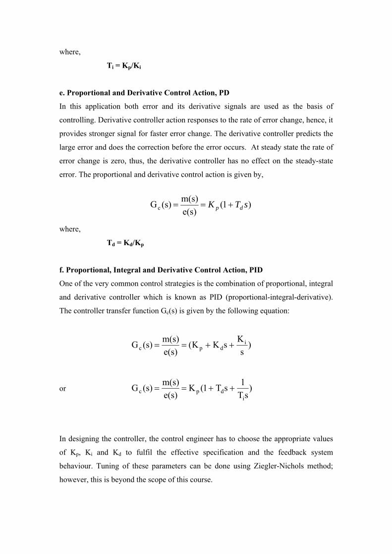
f. Proportional, Integral and Derivative Control Action, PID

One of the very common control strategies is the combination of proportional, integral

and derivative controller which is known as PID (proportional-integral-derivative).

The controller transfer function Gc(s) is given by the following equation:

)s

KsKK(e(s)m(s)(s)G i

dpc ++==

or )sT

1sT1(Ke(s)m(s)(s)G

idpc ++==

In designing the controller, the control engineer has to choose the appropriate values

of Kp, Ki and Kd to fulfil the effective specification and the feedback system

behaviour. Tuning of these parameters can be done using Ziegler-Nichols method;

however, this is beyond the scope of this course.

)1(e(s)m(s)(s)Gc sTK dp +==

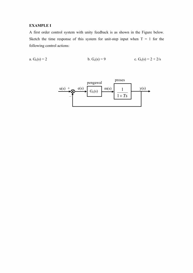
EXAMPLE I

A first order control system with unity feedback is as shown in the Figure below.

Sketch the time response of this system for unit-step input when T = 1 for the

following control actions:

a. Gc(s) = 2 b. Gc(s) = 9 c. Gc(s) = 2 + 2/s

+ _ Ts+1

1

u(s) y(s) e(s) Gc(s)

m(s) pengawal

proses