time-scale modification algorithms for music audio signals · 2011-11-03 · when using analogue...
TRANSCRIPT
Saarland University
Faculty of Natural Sciences and Technology IDepartment of Computer Science
Master’s Thesis
Time-Scale Modification Algorithms
for Music Audio Signals
submitted by
Jonathan Driedger
submitted
November 3, 2011
Supervisor / Advisor
Priv.-Doz. Dr. Meinard Muller
Reviewers
Priv.-Doz. Dr. Meinard Muller
Prof. Dr. Michael Clausen

Eidesstattliche Erklarung
Ich erklare hiermit an Eides Statt, dass ich die vorliegende Arbeit selbststandig verfasstund keine anderen als die angegebenen Quellen und Hilfsmittel verwendet habe.
Statement under Oath
I confirm under oath that I have written this thesis on my own and that I have not usedany other media or materials than the ones referred to in this thesis.
Einverstandniserklarung
Ich bin damit einverstanden, dass meine (bestandene) Arbeit in beiden Versionen in dieBibliothek der Informatik aufgenommen und damit veroffentlicht wird.
Declaration of Consent
I agree to make both versions of my thesis (with a passing grade) accessible to the publicby having them added to the library of the Computer Science Department.
Saarbrucken,(Datum / Date) (Unterschrift / Signature)

Acknowledgments
First of all I would like to express my deepest gratitude to my supervisor Meinard Mullerwho gave me the possibility to work on this compelling topic. I never imagined thatwriting my Master’s Thesis could be that fun, and the fact that it was is mainly due tohim. He always found the time to discuss my ongoing work with me and give me goodadvice.
The next person I would like to thank is Peter Grosche. His dedication to help me, and alsoall other students in the Multimedia Information Retrieval and Music Processing group,is incredible. I can not remember a single time he sent me away when I had some sort ofquestion. He was a constant source of inspiration and motivation for me.
Furthermore, I would like to thank my fellow student and dear friend Thomas Pratzlich,who was writing his Master’s Thesis at the same time as I did, for the hours and hoursof discussions and mutual assistance. It was nice to always have somebody to talk aboutthesis-related problems.
I also would like to thank Verena Konz, Nanzhu Jiang and Marvin Kunnemann for proof-reading my thesis and giving me a lot of feedback as well as Zuo Zhe for helping me withmy experiments.
Last but not least I would like to thank my family and especially my partner Julia Hah-nemann for their support throughout the time of writing this thesis.

Abstract
Sound is a phenomenon that lives in manifold dimensions. Besides pitch, volume, timbreand many others, the time is an essential component. In the field of audio signal processingnot only the analysis of these aspects, and in particular the time aspect, but also theirmodification is an important issue. When sound becomes music, time becomes tempo andrhythm. Having the possibility to change the tempo and the rhythm of audio recordingsis extremely helpful for example when a DJ wants to adapt the tempos of two songs. Butwhen using analogue audio media like records or tapes, changing the playback speed of themusic does not only affect the tempo, but also the pitch of the sound. This looks differentin the world of digital audio recordings where algorithms were invented to decouple thetime-scale of audio signals from their pitch. These are typically referred to as time-scalemodification (TSM) algorithms. But although there exists a large variety of differentalgorithmic approaches to the field of TSM of audio recordings, there is no algorithm thatproduces artifact-free results robustly.
The goal of this thesis is therefore to analyze what makes TSM difficult and where ar-tifacts originate from. We investigate two prominent TSM algorithms, one working inthe time-domain (WSOLA) and one working in the frequency-domain (Phase Vocoder).Both algorithms produce their very own artifacts which we analyze and classify. Usingthe example of WSOLA, we show how to overcome a certain class of artifacts that arefrequently produced by time-domain TSM algorithms at transients in audio signals. Toevaluate the quality of different TSM algorithms we present the results of a listeningtest that we performed. Finally we integrate our knowledge about TSM algorithms intoa soundtrack generation system that allows for creating euphonious transitions betweenaudio recordings.

Contents
1 Introduction 1
1.1 Time-Scale Modification of Audio Signals . . . . . . . . . . . . . . . . . . . 1
1.2 Motivating Application . . . . . . . . . . . . . . . . . . . . . . . . . . . . . . 2
1.3 The Connector . . . . . . . . . . . . . . . . . . . . . . . . . . . . . . . . . . 3
1.4 Contribution . . . . . . . . . . . . . . . . . . . . . . . . . . . . . . . . . . . 4
1.5 Thesis Organization . . . . . . . . . . . . . . . . . . . . . . . . . . . . . . . 5
2 Basic Definitions, Notations and Tools 7
2.1 Audio Signals . . . . . . . . . . . . . . . . . . . . . . . . . . . . . . . . . . . 7
2.2 Pitch Features . . . . . . . . . . . . . . . . . . . . . . . . . . . . . . . . . . 8
2.3 Chroma Features . . . . . . . . . . . . . . . . . . . . . . . . . . . . . . . . . 9
2.4 Beat-Synchronous Chroma Features . . . . . . . . . . . . . . . . . . . . . . 11
3 Time-Scale Modification 13
3.1 Introduction . . . . . . . . . . . . . . . . . . . . . . . . . . . . . . . . . . . . 13
3.2 Related Work . . . . . . . . . . . . . . . . . . . . . . . . . . . . . . . . . . . 15
3.3 General Definitions and Remarks . . . . . . . . . . . . . . . . . . . . . . . . 16
4 WSOLA 21
4.1 OLA . . . . . . . . . . . . . . . . . . . . . . . . . . . . . . . . . . . . . . . . 21
4.2 Improvements to OLA - The WSOLA Algorithm . . . . . . . . . . . . . . . 25
4.3 Artifacts . . . . . . . . . . . . . . . . . . . . . . . . . . . . . . . . . . . . . . 29
5 Phase Vocoder 35
5.1 Short Time Fourier Transform . . . . . . . . . . . . . . . . . . . . . . . . . 35
5.2 Phase Vocoder Pipeline . . . . . . . . . . . . . . . . . . . . . . . . . . . . . 37
5.3 Phase Propagation . . . . . . . . . . . . . . . . . . . . . . . . . . . . . . . . 38
5.4 Modifications for a simple implementation . . . . . . . . . . . . . . . . . . . 41
5.5 Artifacts . . . . . . . . . . . . . . . . . . . . . . . . . . . . . . . . . . . . . . 44
6 Transient Preserving WSOLA 47
6.1 Anchor Points . . . . . . . . . . . . . . . . . . . . . . . . . . . . . . . . . . . 47
6.2 Transient Detection . . . . . . . . . . . . . . . . . . . . . . . . . . . . . . . 48
6.3 Transient Preservation . . . . . . . . . . . . . . . . . . . . . . . . . . . . . . 53
6.4 Limitations of the Transient Preservation . . . . . . . . . . . . . . . . . . . 56
7 Listening Test 63
iii

iv CONTENTS
7.1 Test Dataset . . . . . . . . . . . . . . . . . . . . . . . . . . . . . . . . . . . 637.2 Test Setup . . . . . . . . . . . . . . . . . . . . . . . . . . . . . . . . . . . . . 637.3 Results . . . . . . . . . . . . . . . . . . . . . . . . . . . . . . . . . . . . . . . 66
8 The Connector’s Pipeline 718.1 Related Work . . . . . . . . . . . . . . . . . . . . . . . . . . . . . . . . . . . 728.2 Matching . . . . . . . . . . . . . . . . . . . . . . . . . . . . . . . . . . . . . 738.3 Query Pool . . . . . . . . . . . . . . . . . . . . . . . . . . . . . . . . . . . . 768.4 Database . . . . . . . . . . . . . . . . . . . . . . . . . . . . . . . . . . . . . 798.5 Warping . . . . . . . . . . . . . . . . . . . . . . . . . . . . . . . . . . . . . . 798.6 Blending . . . . . . . . . . . . . . . . . . . . . . . . . . . . . . . . . . . . . . 81
9 Future Work 83
A Source Code 85
B Listening Test Questionnaire 87
C Listening Test Comments 89
D The Connector 93
Bibliography 95

Chapter 1
Introduction
1.1 Time-Scale Modification of Audio Signals
Sound is a phenomenon that lives in manifold dimensions. Besides pitch, volume, timbreand many others, the time is an essential component of audio signals. Being able not onlyto analyze but also to modify aspects of sound is an important issue in the field of audiosignal processing. Therefore also the modification of the time aspect, which is generallyreferred to as time-scale modification (TSM) of audio signals, has received a lot of interest.The task is visualized in Figure 1.1. When sound becomes music, time becomes tempo andrhythm. Having the possibility to change the tempo and the rhythm of audio recordings isextremely helpful for example in the field of DJing when a DJ wants to adapt the temposof two songs. But when using analogue audio media like for example records or tapes,changing the playback speed of the music does not only affect the tempo, but also thepitch of the sound.
This looks different in the world of digital audio recordings where algorithms were inventedto decouple the time-scale of audio signals from their pitch. These are typically referredto as TSM algorithms. But although there exists a large variety of different algorithmicapproaches to the field of TSM of audio recordings, there is no algorithm that produces
TSM
Audio recording New time-axis
Time-scale modified audio recording
Figure 1.1. Basic principle of TSM. TSM algorithms allow for modifying the time-scale of anaudio recording according to a given time-axis.
1

2 CHAPTER 1. INTRODUCTION
artifact-free results robustly. In this thesis we therefore analyze and explain the TSMof audio signals in general as well as prominent existing algorithms to better understandwhat makes TSM difficult and where artifacts originate from. In the next sections we fur-thermore propose a novel application that heavily relies on TSM to motivate this detailedanalysis.
1.2 Motivating Application
When the first movies were created at the end of the 19th century, they had no soundtrack.Nevertheless, they were almost always accompanied by musicians to emphasize the images.Nowadays it is almost impossible to imagine media like movies, computer games, TVshows, commercials, slide shows or even theater performances being presented withoutany audible component. But in the same way in which appropriate music can emphasizemoods and emotions, inappropriate music can decrease the quality of motion picturestremendously. Therefore the proper choice of underlaying music is extremely importantin any visual media. But not only the music itself is crucial. For example at a change inthe scenery of a movie the music should adapt to the images, and optimally the change inthe music should be perceived as natural by the audience.
There exist various general approaches for generating soundtracks. The most common oneis the compositorial approach. In a large movie production the music is most commonlycomposed, performed and recorded for this specific movie. The soundtrack is tailoredto the story and any change in the scenery can be handled explicitly by the composer.Although this approach for sure yields the best results, it is extremely expensive since itinvolves a massive amount of creative work by the composer. Furthermore the recordingprocess is labor-intensive and time consuming. Finally the approach is not very flexible.Once the soundtrack is recorded, greater alterations to the movie are virtually impossible.For the same reason it is difficult to apply this approach to other media like for examplecomputer games where no strict time line of events exists. The composer has to designthe music such that it is possible to repeat it over and over again in passages where thescenery does not change and at the same time offer musical transitions that bridge to themusic for the next passage in the storyline of the game.
An other option is the parametric approach. By parameterizing music in terms of harmony,tempo, dynamics, instrumentation and further aspects it is theoretically possible to utilizea synthesizer to produce music that can adapt fast to the shown images by tuning thegiven parameters. In a scene of high tension the parameters could for example be set toproduce loud, fast and percussive music while in the next moment change to soft and quietmusic in a scene of relief. Although this approach is inexpensive and flexible it has shownthat music which is completely computer-generated tends to sound aesthetically not veryappealing to human listeners.
We therefore propose a novel data-driven approach to overcome the shortcomings of thetwo approaches mentioned above. Our core idea builds on the assumption that nowadayslarge music collections that cover a wide range of moods are widely available. From suchcollections suitable audio clips that correspond well to the visual scenes can be chosen andplayed back while accounting for user specifications. Figure 1.2 visualizes our approach.

1.3. THE CONNECTOR 3
Scene 1 Scene 2
Time
Visual data stream
Audio data stream
Audio 1 Audio 2
Audio 1 Audio 2Transition
Naive approach
Our approach
Current playback position
Figure 1.2. Having a collection audio recordings, the goal is to underlay a visual data streamwith fitting music from this collection such that a transition between two recordings is appealing.In the naive approach we simply cut the current audio recording at the end of Scene 1 and appendsome recording that fits Scene 2. But this leads to abrupt breaks in the music. In our approachwe are looking for an optimal recording in the set of all recording that can be used as underlayingmusic for Scene 2 such that we can compute an euphonious transition from the current recordingto the new recording.
The problem is that a simple concatenation of audio recordings does not suffice to createan aesthetically appealing audio data stream since a change from one audio recording tothe next happens abruptly and may therefore be perceived as unpleasant. The goal istherefore to create smooth transitions between two audio recordings that are as pleasantas possible to the ear of the listener.
Blending is a common technique to make the transition between two audio recordings lessabrupt. By overlaying the two audio recordings by a short time and decreasing the volumeof the ending recording until it is finally not perceivable any more while at the same timeincrease the volume of the starting recording from silence to the normal volume, a smoothtransitions between the two recordings is created. Nevertheless, even when blending fromone recording to another one, the transition is often still not acceptable. This is usuallydue to harmonic and rhythmic differences during the transition phase between the tworecordings.
1.3 The Connector
To overcome those issues and to produce harmonically and rhythmically appealing tran-sitions we developed a tool, called the Connector. Its main purpose is to connect audiorecordings in a harmonic and rhythmic sensitive way such that the transition between twoaudio recordings is not, or only slightly noticeable. Its coarse structure is visualized in Fig-ure 1.3. Given to the Connector are the currently playing audio recording along with aregion in this audio recording were we want to switch to another recording. This region iscalled the transition region. In the first stage, the Connector looks for a region in somerecording in a database that has a similar harmonic progression to the transition region.

4 CHAPTER 1. INTRODUCTION
Database
Audio 1 Audio 2
Transition region
Retreived matchQuery
harmonicallysimilar
rhythmicallysynchronized
TSM
Transition
Audio 1 Audio 2
MATCHING
WARPING
BLENDING
Figure 1.3. The three stages of the Connector.
The goal of this step is to assure that during the transition phase the two recordings thatwill be audible at the same time are harmonically related. Having found a match, theConnector rhythmically synchronizes the transition region with the matched region byaligning the beat positions of both regions temporally. This is done to avoid a chaoticsound that would result from overlaying the two regions without any adaptions. To alignthe beat positions, the two audio recordings are warped along the time-axis in a non-linearfashion using TSM algorithms. Since the transition between the two recordings should beaesthetically appealing it is crucial that the applied TSM algorithm introduces as littleaudible artifacts into the audio recordings as possible. At the end of the warping stage thetwo regions can be regarded both harmonically similar and rhythmically synchronized. Inthe last stage the warped audio recordings are finally blended to finish the transition.
1.4 Contribution
The main contribution of this thesis lies in the detailed analysis of different TSM algorithmsand TSM of audio signals in general. Even though TSM techniques have received a lot ofinterest in recent years, non-linear TSM, which plays an essential role in the pipeline ofthe Connector, seems to be a topic that is often avoided in the literature. Furthermorepublications in this field tend to have very diverse notations and definitions. This thesisbuilds a unified theoretical foundation which allows for understanding TSM algorithms indetail and also carefully addresses the topic of non-linear TSM.

1.5. THESIS ORGANIZATION 5
Furthermore we developed and analyzed an improved version of a standard TSM algo-rithm. The quality of this algorithm as well as several other TSM algorithms was evalu-ated by performing a listening test. The results show that our modified algorithm yieldstime-scale modified audio recordings of significantly better quality in many cases than thestandard version of the algorithm.
Finally, as a practical part of this thesis, a first prototype of the Connector as describedin Section 1.3 was implemented in MATLAB.
1.5 Thesis Organization
This thesis is structured as follows. In Chapter 2 we introduce the foundations that arenecessary to work with audio signals on a theoretical level and that are used frequentlythroughout this thesis. Chapter 3 gives a detailed introduction to the field of time-scalemodification of audio signals on an abstract level, while Chapter 4 and Chapter 5 aredevoted to popular TSM algorithms. In Chapter 6 we discuss our new TSM algorithmand explain it in detail. The listening test which we performed to evaluate the quality ofour new algorithm as well as several other TSM algorithms is presented in Chapter 7. Wegive a description of the Connector in its current state and all of its stages in Chapter8 and close this thesis with a brief outline of future work in Chapter 9.
6 CHAPTER 1. INTRODUCTION

Chapter 2
Basic Definitions, Notations and
Tools
The Connector is supposed to be a tool that is capable of producing euphonious tran-sitions from a currently played audio recording to another. To this end, it has to analyze,interpret and modify the audio recording that is currently played as well as the audiorecordings in the database. These are tasks that are not easily manageable by a machineupfront. We first need mathematical formulations of what music, or in general sound, isand how a machine can work with it. As a start, we mathematically define audio signalsin Section 2.1. Afterwards we focus on the harmonic content of audio signals in Sections2.2, 2.3 and 2.4.
Note that throughout this chapter, as well as in this whole thesis we closely follow thenotations and definitions of [33].
2.1 Audio Signals
We begin with the most basic object the Connector has to deal with, the audio signal.
Definition 2.1 An audio signal is a function f : R→ R, where the domain R representsthe time-axis and the range R the amplitude of the sound wave. Since all real-world audiosignals are time-limited with a duration D, we define T = [0, D) ⊂ R as the domain of thetime-limited signal and assume f(t) = 0 for t ∈ R\T . With the domain being R, such anaudio signal is also referred to as continuous-time (CT) signal.
To be able to actually process audio signals with a machine, the signal needs to be trans-formed into a digital representation. To this end we discretize a given CT signal andtherefore turn it into a discrete audio signal.
Definition 2.2 A discrete audio signal, also called discrete-time (DT) signal, is a func-tion x : Z→ R which is defined on a discrete subset of the temporal domain of a CT signal.Since the discrete signal is time-limited as well, we analogously define T ′ = [1 : N ] ⊂ N.
7

8 CHAPTER 2. BASIC DEFINITIONS, NOTATIONS AND TOOLS
0 1 2 3 4 5
−1
0
1
0 1 2 3 4 5
−1
0
1
(a)
(b)
Figure 2.1. (a) A CT signal. Time is given in seconds. (b) The DT version of the CT signalfrom (a) computed by equidistant sampling with a sampling rate of 10 Hz. Time is also given inseconds.
For x being a discrete audio signal we define length(x) = N . Furthermore we definex[a : b] for a, b ∈ T ′ and a ≤ b to be the discrete audio signal that is the fragment of xdefined on z|z ≥ a and z ≤ b.
Note that in fact the range R of a discrete audio signal is also discretized when convertinga CT signal into a DT signal. Nevertheless we will ignore this detail in the following sinceit does not affect our work.
A standard way to convert a CT signal f into a DT signal x is to sample the CT signal atequidistant points, which is known as equidistant sampling. To this end a fixed samplingperiod ps is defined and we compute
x(n) = f(ps · (n− 1)) , (2.1)
for n ∈ Z. The inverse of the sampling period 1ps
is commonly referred to as the samplingrate of the DT signal and denoted by fs.
2.2 Pitch Features
Waveforms are the most common representation of audio signals. They simply encodethe air pressure variations that the human ear perceives as sound. Nevertheless, thisrepresentation hides a lot of information. While temporal events like volume variations arewell perceivable in the waveform, it is for example almost impossible to get any informationabout the frequency content, and therefore harmonic information about the signal fromthe waveform directly. To analyze an audio signal in terms of a certain aspect of sound,and therefore make this aspect accessible and interpretable for a machine, one first has tofind a way to capture and quantify the desired aspect in the signal in a so called feature.In the context of the Connector we are especially interested in the harmonic content ofaudio signals. A common feature to capture this aspect of sound is the pitch feature. Itassigns to each of the 88 MIDI pitches p = 21 to p = 108 that correspond to the keys of astandard piano a value that quantifies how present the corresponding tone is in the audiosignal at a certain point in time.

2.3. CHROMA FEATURES 9
To obtain a pitch feature from an audio signal x we first apply a suitable bandpass filterfor each pitch p to x. This filter passes all frequencies around the center frequency of thecorresponding pitch p while rejecting all other frequencies. By combining all 88 filters weget an array of filters which is called a pitch filter bank. The magnitude response of thisfilter bank yields 88 subband signals xp for p ∈ [21 : 108].
Since we would like to analyze the harmonic content of an audio signal at a high temporalresolution, the audio signal x is typically divided into a sequence of short overlappingsegments,
S = S1, S2, ..., SN , (2.2)
where N is the length of the sequence and it holds that all segments Sn for n ∈ [1 : N ] areof the same length. The final pitch feature is then computed by measuring the short-timemean square power (STMSP) in each of the subband signals xp within each segment Sn.
STMSP (n, p) =∑
k∈Sn
|xp(k)|2 , (2.3)
with n ∈ [1 : N ] and p ∈ [21 : 108]. Figure 2.2 shows an example of a pitch feature.
2.3 Chroma Features
The pitch features introduced in the previous section capture the harmonic content of audiosignals quite well. But in the context of the Connector they have a major drawback.They do not abstract away from the periodic pitch perception of the human auditorysystem. For a human, two tones for which one of them is a multiple in frequency of theother sound similar. We say they have the same “color” or chroma. In western music thesechroma are denoted by C,C♯, D,D♯, E, F, F ♯, G,G♯, A,A♯ and B while adding a numberlabel in case one wants to refer to a certain tone like A1 = 440 Hz and A2 = 880 Hz.Therefore two audio recordings that have a similar chroma progression should also havesimilar feature sequences. This is not always true for the pitch features.
The idea to overcome this problem is therefore to aggregate all pitches that belong to thesame chroma class in a pitch feature vector. The result is a 12-dimensional feature vectorcalled a chroma vector or chroma feature. To increase the robustness against differences insound intensity or dynamics, the chroma vectors are then usually normalized by replacingevery vector v by
v =v
‖v‖1(2.4)
where
‖v‖1 =12∑
i=1
|v(i)| (2.5)
denotes the ℓ1-norm of v. A sequence of chroma features then expresses the relative energydistribution of the underlaying signal within the twelve chroma bands. Chroma features

10 CHAPTER 2. BASIC DEFINITIONS, NOTATIONS AND TOOLS
0 1 2 3 4 5 6 7
−1
0
1
0 1 2 3 4 5 6 7
30
40
50
60
70
80
90
100
10
20
30
40
50
60
70
(b)
(a)
Figure 2.2. (a) The waveform of the first 8 seconds of Beethoven’s 5th Symphony in an orchestralversion. Time is given in seconds. (b) The pitch feature computed from (a). The segments thatwere used to compute the STMSP have a length of 200 ms and overlap by 100 ms.
2.4. BEAT-SYNCHRONOUS CHROMA FEATURES 11
0 1 2 3 4 5 6 7
−1
0
1
0 1 2 3 4 5 6 7C C#D D#E F
F#G
G#A A#B
0.2
0.4
0.6
0.8
(b)
(a)
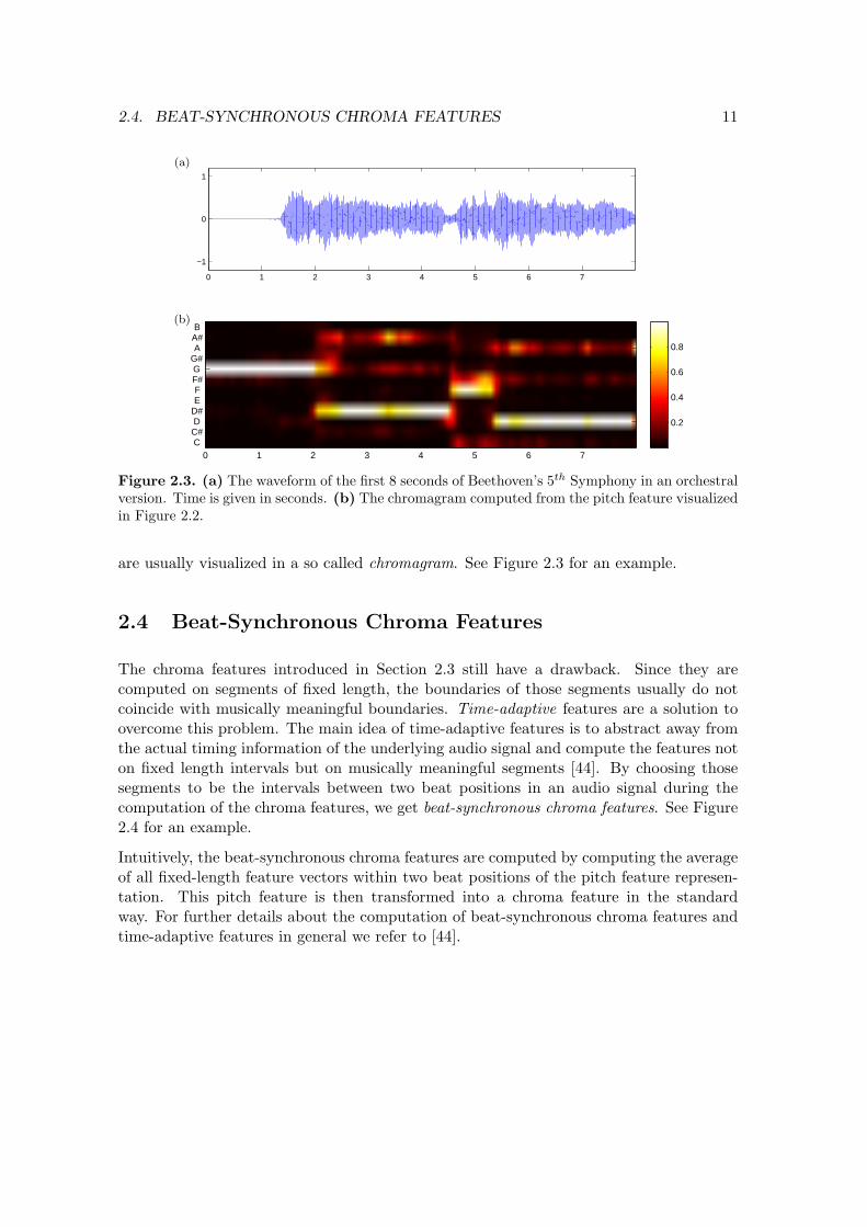
Figure 2.3. (a) The waveform of the first 8 seconds of Beethoven’s 5th Symphony in an orchestralversion. Time is given in seconds. (b) The chromagram computed from the pitch feature visualizedin Figure 2.2.
are usually visualized in a so called chromagram. See Figure 2.3 for an example.
2.4 Beat-Synchronous Chroma Features
The chroma features introduced in Section 2.3 still have a drawback. Since they arecomputed on segments of fixed length, the boundaries of those segments usually do notcoincide with musically meaningful boundaries. Time-adaptive features are a solution toovercome this problem. The main idea of time-adaptive features is to abstract away fromthe actual timing information of the underlying audio signal and compute the features noton fixed length intervals but on musically meaningful segments [44]. By choosing thosesegments to be the intervals between two beat positions in an audio signal during thecomputation of the chroma features, we get beat-synchronous chroma features. See Figure2.4 for an example.
Intuitively, the beat-synchronous chroma features are computed by computing the averageof all fixed-length feature vectors within two beat positions of the pitch feature represen-tation. This pitch feature is then transformed into a chroma feature in the standardway. For further details about the computation of beat-synchronous chroma features andtime-adaptive features in general we refer to [44].

12 CHAPTER 2. BASIC DEFINITIONS, NOTATIONS AND TOOLS
1 2 3 4 5 6 7 8C C#D D#E F
F#G
G#A A#B
0.2
0.4
0.6
0.8
10 20 30 40 50 60C C#D D#E F
F#G
G#A A#B
0.2
0.4
0.6
0.8
0 1 2 3 4 5 6−1
0
1(a)
(b)
(c)
Figure 2.4. (a) The waveform of the first two measures of the song “let it be” from the Beatles.Time is given in seconds and the beat positions are indicated by red bars. (b) The chromagramof the audio signal from (a). The features were computed at a fixed rate of 10 Hz. Again the beatpositions are indicated by red bars. Note that the note boundaries are blurred due to the fixedlength segmentation. (c) The beat-synchronous chromagram computed from the signal from (a)and the beat positions.
Chapter 3
Time-Scale Modification
Time-scale modification is the task of altering the time-scale of audio signals, that meansmaking the tempo of audio recordings faster or slower. In the field of digital signal pro-cessing there exists a large variety of different algorithms that are designed to fulfill thistask. These algorithms are typically referred to as time-scale modification algorithms, orabbreviated by TSM algorithms. While we discuss existing algorithms in Chapters 4, 5and 6 we will address the topic of time-scale modification of DT-audio signals in generalin this chapter. In Section 3.1 we give an introduction to the field of time-scaling of audiosignals. Related work is introduced in Section 3.2 and finally basic definitions as well astechnical remarks are given in 3.3.
3.1 Introduction
The task of manipulating the time-scale of an audio signal is a frequently occurring one.For example in the field of DJing it is often important to have multiple audio clips whichshare the same tempo. A DJ then creates whole songs by overlaying and sequencing thoseclips. For example he could use a drum clip, a bass clip, a melody clip and some effectclips, all played at the same time. But if the drums, the bass and the melody are not onthe same speed level, the result will sound chaotic. He therefore has to take care that thetempos of all simultaneously played clips are the same. But most often audio clips arenot available in different versions for different tempos. The solution is to manipulate thetime-scale of all clips such that they are all on the same speed level.
Another scenario are commercials where an advertising text needs to fit into a predefinedtime frame of mostly 30 or 60 seconds. Since it is extremely difficult for a voice actor tomeet this constraint exactly, the text is most commonly recorded and the speed of theaudio recording is adjusted afterwards such that the length of the recording matches thegiven time. Furthermore, research has shown that the human brain works most efficientlywhen listening to spoken text if the speed of the speaker is about 200 - 300 words perminute [15]. This is the average reading speed of an adult. Unfortunately, the averagerate of speech is in the neighborhood of 100 - 150 words per minute. This fact is usedfrequently in commercials since by speeding up the recorded advertising text one is able
13

14 CHAPTER 3. TIME-SCALE MODIFICATION
to give more information in less time and the faster text is even easier to process by thehuman brain.
These two applications are instances of problems where a simple linear time-scale modifi-cation suffices. For this purpose we can see a TSM algorithm as a method that receivesan audio signal along with some descriptor which describes the intended time-scale mod-ification, in this case a constant time-stretch factor. The time-stretch factor determineshow the time axis of the given audio should be rescaled for the output. For example atime-stretch factor of 2 should yield an audio signal that is twice the length of the audiosignal given to the algorithm. The straightforward approach to realize such a time-scalemodification of an audio signal is to either stretch or compress the waveform of the givenaudio signal, depending on the time-stretch factor. This is done by resampling the givensignal but still interpreting it as a signal sampled at the old sampling rate. Algorithm 1shows how the resampling of a signal can be computed. Unfortunately, this simple ap-proach yields unacceptable results for most applications. When resampling the signal onedoes not only change the time-scale, but also the pitch-scale of the signal at the samerate (see Figure 3.1). The effect is the same as when playing a record or a tape recordingat a higher or lower speed than it is intended to be played. This might be acceptablefor some kinds of audio signals with non-harmonic content, like for example drum beats,where slight changes in the pitch-scale are not directly audible as such. But, for exam-ple, for audio signals containing human voice this leads to the so called chipmunk effect1
which makes the human voice sound completely unnatural and alienated by heighteningor lowering its pitch. In the context of the Connector, the resampling approach is evennot applicable at all since we want to manipulate the time-scale of audio signals that aresimilar in the harmonic sense. A pitch shift destroys this similarity completely.
Algorithm 1: Resampling
Data: DT signal x sampled at a sampling rate fs, time-stretch factor t.Result: DT signal y that is a resampled version of x.begin
z ←− interpolate x to a CT signal;y ←− sample z at a rate of fs · t;
We therefore need TSM algorithms that are capable of changing the time-scale of an audiosignal without altering its pitch-scale. In the optimal case these algorithms should producean audio signal that sounds as if the content of the signal was produced on a differenttime-scale. For example for a musical performance the output should sound as if all themusicians just played at a different tempo.
Historically, the next step towards this goal was to invent the so called Variable SpeechCompression [15]. Having an audio signal, this technique just takes small segments fromthe signal at equidistant positions and either removes them or doubles them. Dependingon the length of those segments and whether they are removed or doubled, the audio signalis more or less shortened or lengthened. This technique was for example implemented incassette recorders. Here, the tape was first played on a higher or lower speed, leading
1http://en.wikipedia.org/wiki/Alvin_and_the_Chipmunks, last consulted in October 2011

3.2. RELATED WORK 15
0 1 2 3 4 5 6 7 8 9 10
−1
0
1
0 1 2 3 4 5 6 7 8 9 10
−1
0
1
x
y
Figure 3.1. The sinusoidal signal x is sampled at a rate of 22050 Hz and has a frequency of1 Hz (the time on the x-axis is given in seconds). By resampling the signal to 44100 Hz we getthe signal y. The length of y is double the length of the signal x, but at the same time also thewavelength of x is doubled. Therefore the frequency of the sinusoidal signal y is 0.5 Hz. It isnot possible to change only the duration of a signal without changing the pitch and vice versa bypurely resampling the signal.
to time-scaled, but pitched signals. Then small segments were recorded from the tape,resampled to pitch them back to their initial pitch and then fed to the output, while eitherskipping certain parts of the tape when increasing the speed or doubling the resampledsegments when slowing the audio down. The quality of time-scaled audio signals producedby variable speech compression was rather good, especially when manipulating the time-scale of speech recordings. But stuttering artifacts were always audible and the approachwas therefore far away from the goal of artifact free time-scale modification. Nevertheless,this technique has a lot in common with one of the first digital TSM algorithms, the OLA(Overlap and Add) technique which we discuss in Chapter 4.
An interesting fact is that pitch-scale modification, which is the task of changing onlythe pitch of an audio signal while the length of the signal is preserved, is actually thesame as time-scale modification. While at the first glance these problems seem unrelated,solving one of them also solves the other. Assume one has a perfect TSM algorithm thatis capable of time-scaling any audio signal without introducing artifacts, but the task isto lower the pitch of an audio signal without altering the length. One starts by usingthe TSM algorithm to shorten the duration of the audio signal without altering its pitch.Afterwards, one uses the naive resampling approach to stretch the shortened signal to itsinitial length again and at the same time lower its pitch. This results in an audio signal,that has the same length as the initial signal but that is lowered on the pitch-scale. Theheightening of the pitch-scale works analogously.
3.2 Related Work
A lot of work has been done and is still ongoing in the field of time-scale modificationof audio signals. The Variable Speech Compression [15] that was briefly introduced inSection 3.1 was one of the first contributions to this field. For modern TSM algorithmsthere exist in principle two main approaches: They either work in the time-domain or in

16 CHAPTER 3. TIME-SCALE MODIFICATION
the frequency-domain.
Algorithms working in the time-domain try, similarly to the Variable Speech Compression,to take small segments from specific positions in the input audio signal and resynthesizethem to a new, time-scale modified version of the input audio signal. Most of these al-gorithms follow a basic scheme, the so called OLA (Overlap and Add) technique. Thistechnique is presented in [36] and is also discussed in detail in Chapter 4. Many highquality TSM algorithms originate from this technique. Examples are the WSOLA algo-rithm (Wave Similarity Overlap and Add) [43], which is also discussed in Chapter 4, theSOLA algorithm (Synchronized Overlap and Add) [37] and the PSOLA algorithm (Pitch-Synchronous Overlap and Add)[32]. These algorithms often suffer from stuttering artifactsat transient regions in audio signals. Therefore the quality of the results can be improvedby giving these transient regions a specialized treatment. An approach to improve thequality of WSOLA can be found in [19] and our own approach is discussed in Chapter 6.
The other family of TSM algorithms works in the frequency-domain. These algorithmsapproach the problem by constructing frequency spectra that correspond to a time-scaledversion of the input audio signal. By transforming these spectra back to the time-domainthey produce the output audio signal. The most prominent algorithm of this family is thePhase Vocoder [14, 1, 9, 10, 42], which is discussed in detail in Chapter 5.
There exist also some hybrid approaches that work partially in the time-, and partially inthe frequency domain. Such algorithms are presented in [25, 18, 11]. A recent and veryintersting approach which combines WSOLA and the Phase Vocoder can be found in [31].
3.3 General Definitions and Remarks
In the context of the Connector, as well as in many other applications it is not sufficientto have a TSM algorithm that only allows for a linear time-scale modification. Often itis necessary to scale the time of an audio signal in a non-linear fashion. For example inthe Connector we want to synchronize the beats of two audio signals. But those beatpositions do not need to be equidistant. In fact, this is not the case in most musicalpieces performed by humans. Not only that unskilled musicians tend to miss the correctbeat position, but also professional musicians often play notes a little bit before or afterthe beat (pushing/lay back) to create certain moods in their music. This is referred toas tempo rubato [23]. Furthermore agogics like ritardando or accelerando (get slower/getfaster) make musicians change the speed of the played piece and therefore the temporaldistance between beats. In such cases a non-linear time-scale modification is necessary tosynchronize the beat positions of two audio recordings.
Modern TSM algorithms are normally capable of handling non-linear time-scale modifi-cations. To this end they get a time-stretch function τ along with the input signal as adescriptor of the intended time-scale manipulation. Intuitively a signal f and a signal gwhich is a time-scale modified version of f with respect to the time-stretch function τshould then satisfy the formula
∀t ∈ [0, T ) : g(τ(t)) = f(t) , (3.1)

3.3. GENERAL DEFINITIONS AND REMARKS 17
where T is the duration of f . This formula states that every single point in time of signalf is mapped to a point in time in g by the time-stretch function τ . Unfortunately theformula does not specify what we intended. Figure 3.2 shows an example of a signal, atime-stretch function and a time-scaled version of the signal which satisfy the formula. Theproblem is that in an audio signal, information about time, pitch, timbre and many otheraspects of sound are mingled together. Formula 3.1 specifies a time-scale manipulationthat manipulates all properties of a signal at once which leads to the same artifacts aswhen speeding up or slowing down the spin of a record according to the time-stretchfunction while playing it, or, in the digital world, the resampling approach discussed inSection 3.1. But our goal is to manipulate only the time axis of an audio signal, withoutchanging any other properties. We therefore have two seemingly contradicting goals. Onthe one hand we want to distort the audio signal temporally on a global scale to achieve theintended time-scale modification, but on the other hand we want to preserve it locally tomaintain aspects like pitch and timbre. To define this property and therefore to overcomethe shortcomings of Equation 3.1 we need a better way to talk about corresponding pointsin time in two signals. We are looking for a relation that allows us to compare the localcontent of two signals at given points in time. Defining such a relation is difficult since it isnot even easy to explain what exactly a point in time in an audio signal is. When we breakit down to the waveform, it is just the displacement in the air pressure at the given time,measured and quantized in the amplitude of the recorded signal. But this informationis not enough to preserve aspects like pitch and timbre of the signal when time-scalemodifying it. The problem is that not a single point in time makes the difference in airpressure that the human ear perceives as sound, but a sequence of different air pressurelevels does. It is therefore necessary that the relation we are looking for does not connectpure points in time, but short time segments.
We now first give the definition of the term time-stretch function.
Definition 3.1 A Time-Stretch Function τ for a CT signal f is a strictly monotonouslyincreasing function τ : [0, T )→ R where T is the duration of f . The domain of τ representsthe time-axis of f and the range the time-axis of a time-scale modified version of f .
To be able to give at least an intuitive definition of what it means that an audio signal fis time-scale modified with respect to a time-stretch function τ we introduce a relation ≈and give it the vague meaning of “similar to”. Note that finding an operational definitionof this relation that describes the desired property perfectly is the same as solving theTSM problem artifact free since we could just use the definition to compute the outputsignal. Therefore building a TSM algorithm is somehow similar to approach the problemof defining this relation.
Definition 3.2 A CT window function w of size ℓ is a function w : R → R such thatw(t) > 0 for all t ∈ T = [− ℓ
2 ,ℓ2) and w(t) = 0 for t ∈ R\T .
Definition 3.3 A CT signal g is a time-scale modified version of a CT signal f withrespect to τ if
∀t ∈ [0, T ) : g(τ(t) + s) · w(s) ≈ f(t+ s) · w(s) ,
where T is the duration of the signal f , w is a window function of window size ℓ ands ∈ (− ℓ
2 ,ℓ2).

18 CHAPTER 3. TIME-SCALE MODIFICATION
Note that in the above definition the relation ≈ relates windowed segments of the twosignals and not single points in time.
Since we want to argue mainly about digital signals we need to adapt the definition to DTsignals.
Definition 3.4 Let x : [1 : N ] → R be a DT signal and τ a time-stretch function fora continous version of x. A Discretized Time-Stretch Function τ of τ for x is a strictlymonotonously increasing function τ : A → [1 : M ] where A ⊆ [1 : N ] 1, N ∈ A and M isthe length of the time-scale modified signal and it holds that
(i) τ(1) = 1
(ii) τ(N) =M
(iii) ∀n ∈ A\1, N : τ(n) = [τ([n]time)]sample
The functions used in (iii) are defined as [n]time = n · ps and [t]sample = round( tps ) whereps is the sampling period of x.
A discretized time-stretch function τ does not need to be defined for all sample positions ofa DT signal x. Nevertheless this is often necessary. We therefore introduce the interpolatedtime-stretch function τ ′.
Definition 3.5 An Interpolated Time-Stretch Function τ ′ of a discretized time-stretchfunction τ for a DT signal x is a monotonously increasing function τ ′ : [1 : N ]→ [1 :M ]where N is the length of x and M is the length of the time-scale modified version of x.The function τ ′ is computed from τ by discrete linear interpolation.
When defining TSM algorithms it is also often necessary to invert the time-stretch function.In the discrete world we therefore have to overcome the problem that the interpolatedtime-stretch function τ ′ is not necessarily strictly monotonously increasing. We define theinverse of an interpolated time-stretch function as follows.
Definition 3.6 An Inverted Interpolated Time-Stretch Function τ ′−1 of an interpolatedtime-stretch function τ ′ for a DT signal x is a monotonously increasing function τ ′−1 :[1 :M ]→ [1 : N ] where N is the length of x and M is the length of the time-scale modifiedversion of x. The function τ ′−1 is computed from τ−1 by discrete linear interpolation.
Finally we adapt Definition 3.3 to the discrete world.
Definition 3.7 A DT window function w of size L is a function w : Z → R such thatw(m) > 0 for all m ∈M = [−⌊L−1
2 ⌋ : ⌊L2 ⌋] and w(m) = 0 for m ∈ Z\M .
Definition 3.8 A DT signal y is a time-scale modified version of a DT signal x withrespect to τ ′ if
∀n ∈ [1 : length(x)] : y(τ ′(n) +m) · w(m) ≈ x(n+m) · w(m) ,
where w is a window function of size L and m ∈ [−⌊L−12 ⌋ : ⌊
L2 ⌋].
3.3. GENERAL DEFINITIONS AND REMARKS 19
0 1 2 3 4 5 6 7 8 9 10
−1
0
1
0 1 2 3 4 5 6 7 8 9100123456789
10
0 1 2 3 4 5 6 7 8 9 10
−1
0
1
(a) (b)
(c)
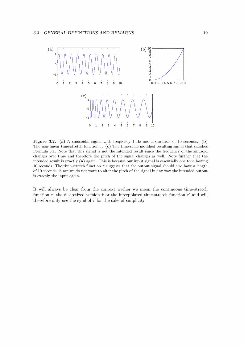
Figure 3.2. (a) A sinusoidal signal with frequency 1 Hz and a duration of 10 seconds. (b)The non-linear time-stretch function τ . (c) The time-scale modified resulting signal that satisfiesFormula 3.1. Note that this signal is not the intended result since the frequency of the sinusoidchanges over time and therefore the pitch of the signal changes as well. Note further that theintended result is exactly (a) again. This is because our input signal is essentially one tone lasting10 seconds. The time-stretch function τ suggests that the output signal should also have a lengthof 10 seconds. Since we do not want to alter the pitch of the signal in any way the intended outputis exactly the input again.
It will always be clear from the context wether we mean the continuous time-stretchfunction τ , the discretized version τ or the interpolated time-stretch function τ ′ and willtherefore only use the symbol τ for the sake of simplicity.
20 CHAPTER 3. TIME-SCALE MODIFICATION

Chapter 4
WSOLA
WSOLA (Wave Similarity Overlap and Add) is a time-domain TSM algorithm from thefamily of OLA algorithms and was first introduced in [43]. In this section we discuss itin detail. We first introduce the basic OLA technique in Section 4.1 and afterwards theimprovements that were done in WSOLA in Section 4.2. Finally we briefly have a look atoccurring artifacts in Section 4.3.
4.1 OLA
The basic OLA technique is very simple and follows roughly the ideas of the VariableSpeech Compression. The main idea of the algorithm is to cut out small segments fromthe input audio and concatenate them by crossfading from one segment to the next toachieve the desired time-scale modification. To be able to describe the technique properlywe first need to introduce some definitions and remarks.
Remark 4.1 We will use window functions massively throughout this chapter. For thesake of convenience we will therefore denote the size of a window function w by wℓ.
Definition 4.1 For x being a DT signal of length N and w being a window function ofsize N , we define
x · w
to be the pointwise multiplication of x and w.
Definition 4.2 A windowed audio segment z from an DT signal x using the windowfunction w around window position p is defined as
z = x[bpw : epw] · w ,
where bpw = p − ⌊wℓ−12 ⌋ is the beginning of the windowed audio segment z in x and epw =
p+ ⌊wℓ2 ⌋ is the end of the windowed audio segment z in x.
21

22 CHAPTER 4. WSOLA
Definition 4.3 Let w be a window function. In a sequence of windows in which allwindows can be described by a shifted version of w and in which all windows are overlappingby a constant factor o we call the distance between the centers of two adjacent windowsthe standard window offset ηwo and compute it as
ηwo = (1− o) · wℓ .
Given to the OLA algorithm are an input signal x, an overlap factor o, a window functionw and a time-stretch function τ . The goal of the algorithm is to produce an audio signaly that is a time-scale modified version of x with respect to τ . The OLA technique realizesthis task by copying audio segments that are windowed using w from the input signal xto the output signal y. It is important that the size of the used window function w islonger than one pitch period of the lowest fundamental frequency contained in the inputsignal x, since a windowed audio segment from x using w should contain harmonicallymeaningful content. In the output these windowed audio segments are overlapped by theconstant overlap factor o and added up, which yields a crossfade from one segment to thenext. This procedure is the origin of the name of the technique (Overlap and Add).
The first step of the OLA technique is to generate a vector of output window positions γ.This vector specifies positions where the windowed audio segments from the input will beplaced in the output. It is fully determined by the length of the output signal y (which byitself is given by the time-stretch function τ), the length of the window function wℓ andthe overlap factor o. This is because it specifies the positions of a sequence of windowsthat are all overlapping by the same factor. Therefore all entries in γ are equidistant anddepend only on wℓ and o. The length of γ is determined by the length of y since no windowposition in γ may exceed the length of y.
Now we can compute γ by
(i) length(γ) = ⌈ length(y)ηwo⌉
(ii) γ(1) = 1(iii) γ(n) = γ(n− 1) + ηwo for n ∈ [2 : length(γ)]
(4.1)
One can now imagine the output signal y as a sequence of slots that need to be filled withwindowed audio segments from the input. The positions of these slots are all equidistantand given by γ. To fill these slots with windowed audio segments such that the outputsignal y is a time-scale modified version of x with respect to the time-stretch function τ ,we construct a vector of input window positions σ which is dependent on τ . It is computedby
σ(n) = τ−1(γ(n)) (4.2)
for all n ∈ [1 : length(γ)]. Every slot in y specified by γ(n) is then filled with the windowedaudio segment at window position σ(n). Figure 4.1 gives a visual example of how the OLAtechnique works.

4.1. OLA 23
0
1
Inpu
t Aud
io
0
1
Out
put A
udio
σ(1) σ(2) σ(3) σ(4) σ(5)
γ(1) γ(2) γ(3) γ(4) γ(5)
ηwo
Figure 4.1. Schematic mechanics of OLA. Signals are symbolized by blue bars. The input signalis windowed at specified positions σ. The resulting windowed segments are then overlapped by aconstant factor o (it holds that γ(n+ 1)− γ(n) is constant, in this case the overlap factor o is 0.5and the standard window offset ηwo therefore is half the window size), added up and copied to theoutput. The example shows how OLA produces a version of the input signal that is speeded up bya constant factor (the windows in the input are sampled equidistantly along the input signal andσ(n+ 1)− σ(n) > γ(n+ 1)− γ(n)).
Mathematically we can describe the synthesis of y as
y(n) =
length(σ)∑k=1
w(n− γ(k)) · x(n− γ(k) + σ(k))
length(σ)∑k=1
w(n− γ(k))
. (4.3)
Intuitively Equation 4.3 simply computes the sum of all windowed audio segments fromthe input signal x that contribute to sample position n in the output signal y. Note thatthe denominator is used to normalize the output y at position n in case the overlappingwindows at position n in the output do not add up to 1. This normalization is importantto avoid amplitude modulations in the output signal y (see Figure 4.2 for an example).In OLA techniques, the overlap factor o is typically set to 0.5 and the window function wusually describes a Hann-window. With these settings the denominator of Equation 4.3is always 1.
From Equation 4.3 we can derive Algorithm 2. Note that the very last step of the algorithmapplies the discussed normalization to the output signal y and is obsolete in case o = 0.5and w being a Hann-window.
By extracting and rearranging small segments with harmonically meaningful content fromthe input audio x, the OLA technique tries to give the relation ≈ that we introduced inChapter 3 the meaning of “harmonically similar to”. The Short Time Fourier Transform

24 CHAPTER 4. WSOLA
0
1
0
0.5
1
1.5
2
0
1
0
0.5
1
1.5
2(a)
(b)
(c)
(d)
Figure 4.2. (a) and (b) The Hann-windows in (b) are overlapped by an overlap factor ofo = 0.5. The plot in (a) shows the pointwise addition of all windows. The summed values areconstantly equal to 1. (c) and (d) The Hann-windows in (d) are overlapped by an overlap factorof o = 7
10 . The plot in (c) shows the pointwise addition of all windows. One can observe thatsummed values are not constant. Note that the function plots shown in (a) and (c) describe exactlythe denominator of Equation 4.3 if we assume that w is the used Hann-window function and thewindow positions resulting from the overlap factors are given in a vector γ.
Algorithm 2: OLA
Data: DT signal x, window function w, overlap factor o, time-stretch function τ .Result: DT y that is a time-scale modified version of x.begin
/* Compute γ */
γ(1) = 1;
for i← 2 to ⌈ length(y)ηwo⌉ do
γ(i)←− γ(i− 1) + ηwo ;
/* Compute σ */
for i← 1 to length(γ) doσ(i)←− τ−1(γ(i));
/* Overlap and Add */
for j ← 1 to length(σ) do
frame←− x[bσ(j)w : e
σ(j)w ] · w;
y[bγ(j)w : e
γ(j)w ]←− y[b
γ(j)w : e
γ(j)w ] + frame;
/* Adjust possible amplitude modulations */
y ←− adjustAmplitude(y, w, o)

4.2. IMPROVEMENTS TO OLA - THE WSOLA ALGORITHM 25
[26] is a tool to analyze the frequency content of a DT signal. It is defined by
X(t, k) =∑
n∈Z
x(t+ n) · w(n) · e−2·π·i·k·n
N , (4.4)
where N is the size of the discrete Fourier Transform, w is a window function of size N , tis the time given in samples and k is the index of the frequency bin with center frequency2·π·kN . Let Xν be defined as
Xν = (X(ν(1), ·), X(ν(2), ·), ..., X(ν(Z), ·)) , (4.5)
where ν is some vector of sample positions of length Z. We can therefore describe theinstantiation of ≈ that OLA is designed to fulfill as
∀n ∈ [1 : length(x)] : y(τ(n) +m) · w(m) ≈ x(n+m) · w(m) :⇔Yν ≈LS Xτ−1(ν)
(4.6)
where ≈LS means “close to” in the least-squares sense, w is a window function of size Land m ∈ [−⌊L−1
2 ⌋ : ⌊L2 ⌋]. Equation 4.6 defines that the harmonic content of the input and
the output signal have to be similar at a given set of pairs of points in time((ν(1), τ−1(ν(1))
),(ν(2), τ−1(ν(2))
), ...,
(ν(Z), τ−1(ν(Z))
)), (4.7)
where the first entry of a pair specifies a point in time in the output signal and the secondentry a point in time in the input signal. If we instantiate ν with γ, OLA fulfills thisdefinition by design since the window positions in OLA are chosen exactly this way (recallthat we calculated σ as σ(n) = τ−1(γ(n)).
The quality of audio signals created with the OLA technique is acceptable as long asthe content of the signal is of a non-harmonic nature like for example speech. But whenit comes to the time-scaling of signals with harmonic content, like for example musicrecordings, the technique introduces a lot of modulation artifacts. These artifacts resultfrom cancellation effects that occur when the phases of the fundamental frequencies of twooverlapping windows in the output do not match. This also introduces most certainly phasejumps (see Figure 4.3) which then lead to a dissonant sound of the output signal. This isof course not acceptable in most scenarios where music should be time-scale manipulated.The reason for the occurring artifacts is that the instantiation of ≈ described in Equation4.6 which OLA fulfills is not sensitive to the phase relationships existing in the the inputsignal x. It is therefore necessary to revise this definition.
4.2 Improvements to OLA - The WSOLA Algorithm
The problem with basic OLA is that the technique is not sensitive to the input signal itself.It just copies windowed audio segments from fixed positions in the input audio signal tofixed positions in the output audio signal. The underlying signal has no influence on the

26 CHAPTER 4. WSOLA
−1
0
1
−1
0
1
x(n)
y(n)
Figure 4.3. The input signal x is a simple sinusoid. The signal is stretched using the OLAtechnique by a factor of 2. OLA is not capable of maintaining the structure of x and introducesmodulation and phase jump artifacts into the output signal y.
algorithm at all. Admittedly the frequency content is maintained locally, but so are thephases of the copied segments. When overlapping those segments, artifacts are introducedin case that the phases do not match. The main idea of high quality TSM algorithmsis therefore to keep only the magnitude spectra similar locally while taking care that nonew phase jumps are introduced (optimally phase jumps that existed in the input signalx should persist in the output signal y) instead of maintaining the similarity of the fullFourier spectra (recall that a Fourier spectrum can be divided into a magnitude spectrumand a phase spectrum since a Fourier spectrum is a vector of complex numbers). Wecan therefore define a new instantiation of ≈ which most modern TSM algorithms aim tofulfill.
∀n ∈ [1 : length(x)] : y(τ(n) +m) · w(m) ≈ x(n+m) · w(m) :⇔(i) |Yν | ≈LS |Xτ−1(ν)|(ii) No new phase jumps are introduced in y
(4.8)
where ν is some vector of samplepositions in y, w is a window function of size L andm ∈ [−⌊L−1
2 ⌋ : ⌊L2 ⌋].
In OLA, the artifacts mainly result from discontinuities in the phase of the fundamentalfrequency of the signal. The basic idea to overcome this issue in most time-domain TSMalgorithms is to give the algorithm some flexibility when it comes to the arrangementof the windows such that the fundamental frequency is maintained as well as possible.WSOLA therefore introduces a position tolerance ∆max for the input window positionsspecified by σ and therefore relaxes the time-stretch function τ . But even though WSOLAtherefore deviates from the given time-stretch function τ , it yields results of much betterquality since audio artifacts are reduced significantly and the tiny deviations from τ canbe neglected in practice. For an example compare Figure 4.3 to Figure 4.4.
We define our new input window position vector as
σrelaxed(k) = σ(k) + ∆k , (4.9)
where k ∈ [1 : length(σ)] and ∆k ∈ [−∆max : ∆max]. The WSOLA synthesis equation

4.2. IMPROVEMENTS TO OLA - THE WSOLA ALGORITHM 27
−1
0
1
−1
0
1
x(n)
y(n)
Figure 4.4. The same input signal as in Figure 4.3 is stretched by a factor of 2 using the WSOLAtechnique. WSOLA is able to maintain the sinusoidal structure of the input signal.
Inpu
t Aud
ioO
utpu
t Aud
io
σ(k − 1) + ∆k−1σ′(k − 1) σ(k) σ′(k)
∆k
∆max
ηwo
maximal similar
γ(k − 1) γ(k)
Figure 4.5. One iteration of the WSOLA algorithm. Like in Figure 4.1 signals are symbolized byblue bars. The windowed audio segment around σ(k − 1) is copied to the output. WSOLA nowfinds an offset ∆k ∈ [−∆max : ∆max] (the borders of the tolerance region are indicated by greenlines) for the next window position σ(k) such that the windowed audio segment around σ(k) +∆k
is maximal similar to the windowed audio segment around the natural progression σ′(k−1). Afterhaving found the offset ∆k the windowed audio segment around σ(k)+∆k is copied to the outputand the process is repeated for the next input window position. Note that for the sake of claritythe input window positions are spaced very far apart in contrast to Figure 4.1.
therefore becomes
y(n) =
length(σ)∑k=1
w(n− γ(k)) · x(n− γ(k) + σ(k) + ∆k)
length(σ)∑k=1
w(n− γ(k))
. (4.10)

28 CHAPTER 4. WSOLA
It remains to show how the ∆k are found. Figure 4.5 visualizes the process while it isexplained in detail in the following. Remember that we want to choose the input windowpositions such that the phase of the fundamental frequency of the input signal is preservedas good as possible. In the optimal case we find an offset ∆k such that when overlappingthe windowed audio segment around σ(k) + ∆k with the windowed audio segment atσ(k − 1) + ∆k−1 we have no cancellation effects at all. Unfortunately, this is in generalonly the case if
σ(k) + ∆k = σ(k − 1) + ∆k−1 + ηwo . (4.11)
In this scenario the distance between the two input window positions is the standardwindow offset ηwo . This is by design of WSOLA also the distance between the centers ofoverlapping windowed audio segments in the output. The overlapping parts of the twowindowed audio segments in the output therefore have exactly the same phase since theyorigin from exactly the same segment in the input signal. We therefore call the sampleposition σ(k − 1) + ∆k−1 + ηwo the natural progression σ′(k − 1) of the sample positionσ(k − 1) + ∆k−1 and generally define it by
σ′(k) = σ(k) + ∆k + ηwo . (4.12)
Note that in case Equation 4.11 holds for all k ∈ [1 : length(σ)] this indicates a time-stretchfunction that is the identity and therefore a global time-stretch factor of 1. In case thetime-stretch function τ is not the identity, the natural progression of σ(k− 1)+∆k−1 willmost probably not lie in the tolerance region [σ(k)−∆max : σ(k)+∆max]. Therefore we arelooking for an offset ∆k ∈ [−∆max : ∆max] such that the windowed audio segment aroundσ(k) + ∆k is as similar as possible to the windowed audio segment around the naturalprogression of σ(k − 1) + ∆k−1. Note that here the term similar indeed means pointwisesimilarity. This offset can therefore be found efficiently by using the cross-correlationmeasure.
The cross-correlation for two DT signals x and y is defined by
(x ∗ y)(n) =∞∑
m=−∞
x(m) · y(n+m) , (4.13)
where x is the complex conjugate of x. Intuitively the measure shifts the signal y by nsamples and computes the sum of the product of x and the shifted y. If a shifted versionof y is similar to x, then positive and negative amplitudes of the two signals are roughlyaligned which yields high values for the product of the two signals and therefore a highvalue of the sum. In contrary, if x is not similar to the shifted version of y, positive andnegative amplitudes will cancel out to a high extend and therefore leave the sum of theproducts small. A peak in the cross-correlation at position n therefore indicates that whenshifting the signal y by −n, the overlapping parts of the signals x and y can be consideredsimilar. In the context of WSOLA we can apply this measure as follows. Having the lastinput window position fixed at σ(k − 1) + ∆k−1 (∆1 is always 0, therefore there alwaysexists a k such that the (k − 1)th window position is already fixed) we are now lookingfor the ∆k such that the windowed audio segments around σ′(k − 1) and σ(k) + ∆k areas similar as possible. In other words we are looking for an offset ∆k ∈ [−∆max : ∆max]
such that x[bσ′(k−1)w : e
σ′(k−1)w ] is as similar as possible to a subsegment of length wℓ in

4.3. ARTIFACTS 29
σ(k)∆k
∆max wℓ ∆max
σ′(k − 1)(a)
(b)
(c)
Figure 4.6. (a) The audio segment around the natural progression of σ(k − 1) + ∆k−1. We can
write it as x[bσ′(k−1)w : e
σ′(k−1)w ]. The position σ(k − 1) + ∆k−1 is the last fixed input window
position. (b) The segment x[bσ(k)w −∆max : e
σ(k)w +∆max]. In this segment we are looking for a
subsegment of length wℓ that is as similar to the segment from (a) as possible. This subsegment,found using the cross-correlation from (c), is marked in red.(c) The cross-correlation of the twosegments. Picking the highest peak from the cross-correlation yields the offset of the segment from(a) to the segment from (b) such that they are as similar as possible. From this offset we cancompute ∆k.
x[bσ(k)w −∆max : e
σ(k)w +∆max]. We now can simply compute the cross-correlation of those
two audio segments. Picking the maximizing index of the cross-correlation yields an offset,and therefore an ∆k, that yields the intended similarity. Figure 4.6 visualizes this process.
Note that the cross-correlation is similar in nature to the convolution and can thereforebe computed efficiently in the frequency domain exploiting that
x ∗ y = x · y , (4.14)
where z is the Fourier spectrum of the signal z.
By using the cross-correlation measure we can finally construct the iterative WSOLAalgorithm (Algorithm 3). Figure 4.5 visualizes one iteration of WSOLA.
4.3 Artifacts
The most typical artifacts occurring in audio signals that were produced by WSOLAare stuttering artifacts. Most often they are audible at transient regions in an audiosignal. Transients are very short, noise-like parts in audio signals that typically originatefrom instrument onsets like for example the stroke of a guitar string or a drum hit. At

30 CHAPTER 4. WSOLA
Algorithm 3: WSOLA
Data: DT signal x, window function w, overlap factor o, time-stretch function τ ,window position tolerance ∆max.
Result: DT y that is a time-scale modified version of x.begin
/* Compute γ */
γ(1) = 1;
for i← 2 to ⌈ length(y)ηwo⌉ do
γ(i)←− γ(i− 1) + ηwo ;
/* Compute σ */
for i← 1 to length(γ) doσ(i)←− τ−1(γ(i));
∆1 ←− 0;for k ← 2 to length(σ) do
/* Overlap and Add */
frame←− x[bσ(k−1)+∆k−1w : e
σ(k)+∆kw ] · w;
y[bγ(k−1)w : e
γ(k−1)w ]←− y[b
γ(k−1)w : e
γ(k−1)w ] + frame;
/* Find next offset */
σ′(k − 1)←− σ(k − 1) + ∆k−1 + ηwo ;
frameAdj ←− x[bσ′(k−1)w : e
σ′(k−1)w ];
frameNext←− x[bσ(k)w −∆max : e
σ(k)w +∆max]
∆k ← getOffsetViaCrossCorrelation(frameAdj,frameNext);
/* Adjust possible amplitude modulations */
y ←− adjustAmplitude(y, w, o)

4.3. ARTIFACTS 31
−1
0
1
−1
0
1
−1
0
1
(a)
(b)
(c)
Figure 4.7. (a) The audio signal of a signal drum hit. The WSOLA input windows for a constanttime-stretch of factor 2 are displayed. (b) The input windows after computing the offsets ∆n forall windows. (c) The resulting audio signal. When listening to the audio signal one hears that thetransient originating from the drum hit is repeated two times. The regions in the signal that arerelated to the repetitions are marked by green boxes.
such positions, a lot of energy is spread all over the frequency spectrum. Especially whenstretching the signal at such a position with a large local time-stretch factor, the density ofinput window positions is high, and therefore this short moment of high energy is containedin several windowed audio segments. When WSOLA copies the windowed audio segmentsto the output, the short burst of energy is audible several times because of the temporalrespacing of the windowed audio segments. Figure 4.7 shows an example of an occurrenceof such a stuttering artifact.
Another interesting artifact occurs in case the wavelength of the fundamental frequencyof the input signal x is at some point larger than the used window length. In this case asingle windowed audio segment does not contain enough information to describe the localcontent of the signal since it is not possible to determine from this windowed audio segmentthe fundamental frequency that is contained in the signal. The task of finding a windowoffset that minimizes phase jumps in the fundamental frequency therefore degenerates tothe task of just keeping the signal locally the same to the input signal. But we alreadysaw that this approach does not yield the intended results and introduces pitch artifactsinto the signal (see Equation 3.1 and Figure 3.2). An example of an instance in which thisartifact occurs can be seen in Figure 4.8.
WSOLA has particular problems when time-scale modifying input signals which are highly

32 CHAPTER 4. WSOLA
0 0.5 1 1.5 2
−1
0
1
0 0.5 1 1.5 2
−1
0
1
x(n)
y(n)
Figure 4.8. The input signal x is a sinusoidal signal with a frequency of 10 Hz, sampled at 22050Hz. The signal is stretched using WSOLA by a factor of 2. The used window length is 2048samples which is slightly less than the wavelength of the sinusoid which is 2205 samples. One cansee that output signal y has a fundamental frequency of 5 Hz and is therefore pitch shifted.
polyphonic, like for example recordings of orchestral music. For such input signals theoutput often soundsmetallic and noisy. This is due to the algorithm’s core idea of choosingthe input window positions such that phase jumps in the fundamental frequency of thesignal are avoided. In case there is more than one fundamental frequency in the inputsignal, only one of them can be preserved properly. The phase continuity of the remainingfundamental frequencies is destroyed and many phase jumps are introduced into the outputsignal what results in the noisy sound.
A forth class of artifacts concerns the timbre of audio signals. The timbre of an instrumentis not only dependent on the overtone spectrum of the sound but also on slight modulationeffects introduced by the instrument. For example the typical sound of a violin has a vibrato(periodic modulation of the pitch of the signal) whereas the sound of a flute is influencedby a tremolo (periodic modulation of the amplitude of the signal). These effects, andespecially the frequency of the modulation, are a natural component of the sound of thoseinstruments. Manipulating the time-scale of a recording containing these instrumentsalso alters the frequency of the vibrato or tremolo effect. As a result the sound of thoseinstruments sounds unnatural (see Figure 4.9).
A related artifact can be observed if an instrument is recorded playing in a wide hall likefor example in a church. The sound of the instrument is reflected on the walls of the halland therefore perceived several times. This effect is called reverb and it is a natural partof our sound perception. In fact the human auditory system is able to estimate the size ofa room based on the reverb of sound sources in the room. Stretching an audio recordingwith noticable reverb for example by a factor of two also doubles the delay times betweenthe sound of the original source and its reverb. When listening to the stretched audiosignal it therefore sounds as if the room in which the audio signal was recorded was largerthan it actually is. These kind of artifacts are not only typical for WSOLA but for anyTSM algorithm.

4.3. ARTIFACTS 33
0 1 2 3 4
0 1 2 3 4
0 1 2 3 4 5 6 7 8
0 1 2 3 4 5 6 7 8
0 1 2 3 4
0 1 2 3 4
0 1 2 3 4 5 6 7 8
0 1 2 3 4 5 6 7 8
(a)
(b)
(c)
(d)
(e)
(f)
(g)
(h)
Figure 4.9. (a) The waveform of a flute playing a single note. (b) The spectrogram related to (a).The tremolo effect of the flute sound manifests itself as equidistant small vertical gaps in the energydistribution. (c) The waveform of a violin playing a single note. (d) The spectrogram relatedto (c). The vibrato effect of the violin sound can be observed as slight temporal pitch vibrationsof a constant frequency. (e) The waveform from (a) stretched using WSOLA by a factor of two.(f) The spectrum related to (e). Note that the fundamental frequency of the signal as well as itsovertone spectrum stayed untouched whereas the gaps in the spectrum that originated from thetremolo were respaced. This leads to a tremolo that is half as fast as in the original signal. (g)The waveform from (c) stretched using WSOLA by a factor of two. (h) The spectrogram relatedto (g). Again note that the frequency content was not altered during the time-scale modificationbut the vibrato is now on half the original tempo.

34 CHAPTER 4. WSOLA

Chapter 5
Phase Vocoder
The most prominent frequency-domain TSM algorithm is the Phase Vocoder [14, 1, 9,10, 42]. It was initially designed to encode the sound of the human voice (therefore theabbreviation vocoder for voice encoder) such that in a communication scenario as littledata as possible needs to be transmitted. Nevertheless, it showed that it was also possibleto alter the time-scale of the encoded signal by manipulating the encoding. The mostimportant tool of the Phase Vocoder is the Short Time Fourier Transform which we discussin Section 5.1. Afterwards we describe the high level pipeline of the algorithm in Section5.2 whereas the core technique of the Phase Vocoder, the so called phase propagation isdiscussed in Section 5.3. Finally in Section 5.4 we develop some modifications to thealgorithm, which are based on the Phase Vocoder implementation of [12], that make theimplementation easier and close with a brief analysis of occurring artifacts in Section 5.5.
5.1 Short Time Fourier Transform
The Short Time Fourier Transform, or short STFT, is an algorithm to analyze a signal interms of frequency composition while at the same time keeping some temporal information,and the most important tool of the Phase Vocoder. We already introduced it briefly inEquation 4.4 but we will restate it here for the sake of convenience. The STFT is definedas
X(t, k) =∑
n∈Z
x(t+ n) · w(n) · e−2·π·i·k·n
N , (5.1)
where t is the analysis instance given in samples, w is the analysis window function, Nis the size of the discrete Fourier Transform and and k is the index of the frequency binwith center frequency 2·π·k
N . In the context of the Phase Vocoder a frequency bin is alsocalled a vocoder channel. Further we define that
Xt = X(t, ·) (5.2)
35

36 CHAPTER 5. PHASE VOCODER
Im
Re∠Q
|Q|
Q
Figure 5.1. The complex value Q = X(t, k) can be seen as a point given in rectangular coordinates(Re(Q), Im(Q)). To get the phase and the magnitude of the partial in vocoder channel with indexk at analysis instance t we change the representation to polar coordinates. We compute the phase
by ∠Q = arctan(
Im(Q)Re(Q)
)and the magnitude |Q| =
√(Re(Q))2 + (Im(Q))2. It always holds that
the phase ∠Q ∈ [−π, π).
is the Fourier spectrum at analysis instance t and
Xν = (Xν(1), Xν(2), ..., Xν(M)) (5.3)
for some vector of analysis instances ν of length M . We write Xν(n) to denote the nth
spectrum in the sequence Xν and Xν(n, k) for its value in the vocoder channel with indexk.
Note thatX(t, k) for some analysis instance t and and vocoder channel index k is a complexvalue. The magnitude |X(t, k)| quantifies how much the partial in the vocoder channelwith center frequency 2·π·k
N contributes to the signal x around the analysis instance t. Itis computed as
|X(t, k)| =√(Re(X(t, k)))2 + (Im(X(t, k)))2 . (5.4)
Furthermore the complex value X(t, k) also encodes the phase of that partial. This phaseis denoted by ∠X(t, k) and can be computed as
∠X(t, k) = arctan
(Im(X(t, k))
Re(X(t, k))
). (5.5)
See Figure 5.1 for an example. The operators | · | and ∠· may also be applied to matriceswhere the application is defined element-wise.
We now come to the inverse of the STFT. Typically the STFT is applied to an audio signalx using a vector of analysis instances α. This yields the sequence of Fourier spectra Xα.

5.2. PHASE VOCODER PIPELINE 37
But in the context of the Phase Vocoder it is very likely that we do not want to apply theinverse Short Time Fourier transform (iSTFT) to Xα directly but to some modificationof it. We therefore generalize the iSTFT. Let Z ∈ CM×N be some sequence of Fourierspectra of length M . Note that Z does not need to be the STFT of any audio signal. Toinvert the STFT we apply the inverse Fourier Transform to each Fourier spectrum in Zand concatenate the resulting audio fragments. We can compute the jth audio fragmentof the output signal y by
yj(n) = Re
(1
N
N−1∑
k=0
Z(j, k) · e2·π·i·k·n
N
). (5.6)
From these partial signals we can construct the output by a simple overlap and add. Toavoid modulation artifacts, a synthesis window w is applied to the signal fragments beforeadding them up. Let β be a vector of synthesis instances given in samples which is oflengthM . The vector β defines where the audio fragments that are computed by Equation5.6 are placed in the output signal.
y(n) =M∑
m=1
w(n− β(m)) · ym(n− β(m) +⌈wℓ2
⌉+ 1) . (5.7)
In case that Z = X(α, k) is the STFT of a signal x for synthesis instances α and it holdsthat α = β, the signal x and the signal y are identical up to minor artifacts introduced bythe used synthesis window w.
5.2 Phase Vocoder Pipeline
Given to the Phase Vocoder are an input signal x together with a time-stretch functionτ . The main idea of the Phase Vocoder is to construct a sequence of appropriate Fourierspectra from x such that applying the iSTFT to this sequence yields the intended time-scalemodification of x. Although it may not appear obvious at first sight, the basic mechanicsof the Phase Vocoder are similar to those of WSOLA: it strives to construct a sequenceof audio fragments from the input signal such that overlap-adding those audio fragmentsyields an output signal that is the time-scale modified input signal. The difference is thatthe Phase Vocoder preserves phase continuity not by small modifications of the fragmentpositions but by manipulating the Fourier spectra of the fragments such that the phasesof consecutive signal fragments match. Nevertheless the basic mechanics of WSOLA andthe Phase Vocoder have a lot in common. Therefore also the internal representations ofthe time-stretch function τ are similar in both algorithms. While WSOLA computes anoutput window position vector γ and an input position vector σ from τ , the Phase Vocoderproduces a vector of synthesis instances β and a vector of analysis instances α. For the

38 CHAPTER 5. PHASE VOCODER
moment the vectors α and β are computed exactly like σ and γ respectively, namely by
(i) length(β) = ⌈ length(y)ηwo⌉
(ii) β(1) = 1(iii) β(n) = β(n− 1) + ηwo for n ∈ [2 : length(β)]
(5.8)
and
α(n) = τ−1(β(n)) (5.9)
for all n ∈ [1 : length(β)]. Note that w describes the analysis window of the STFT in thiscase and the overlap factor o is some fixed constant. Nevertheless we will discuss somechanges to the Phase Vocoder which will simplify its implementation but will also affectthe definitions of α and β in Section 5.4.
The first step of the algorithm is to compute the STFT of x at the analysis instances α.This yields the sequence of frequency spectra Xα. Unfortunately if we now compute theoutput signal y by applying the iSTFT to Xα using the synthesis instances β we run intothe same problems as with the basic OLA technique: by not taking care of the phasesof the partials we get phase jump artifacts in the output. Therefore we have to adjustthe phases of all partials in the Fourier spectra Xα before applying the iSTFT. This stepinvolves a technique called phase propagation which is discussed in detail in Section 5.3.It yields the phase adjusted sequence of Fourier spectra which we denote by X. Finally,applying the iSTFT to X using the synthesis instances β yields the time-scale modifiedoutput signal y. The several stages of the Phase Vocoder are visualized in Figure 5.2.
The Phase Vocoder realizes time-scale modification of audio signals by maintaining localsimilarity of the magnitude spectra of the input and output spectra and at the sametime keeping the phase of all partials of the output signal continuous. It is therefore, likeWSOLA, an approach to fulfill the instantiation of ≈ given in Equation 4.8.
5.3 Phase Propagation
Having a sequence of Fourier spectra Xα we now need to think about how to changethe phases of all the partials in all vocoder channels such that no phase jumps occurwhen copying the audio signal fragments, that result from applying the inverse FourierTransform to the spectra, to the output signal at synthesis instances β. The core idea isthe following: Given a discrete sinusoidal wave with angular frequency ω and phase ϕ atsome sample point n. We now want to know which phase this sinusoidal wave will have atpoint m where m > n. But knowing the frequency ω and the phase ϕ makes this simple.The value (m− n) ·ω gives us the phase increment of the sinusoidal wave from point n topoint m. Therefore the phase of the sinusoidal wave at m will be ϕ+(m−n) ·ω (we needto shift this value to the range of [−π, π) such that it is a valid phase). This is exactlywhat we want to know in the Phase Vocoder: For our first spectrum we do not need toadapt any phases and we can therefore set X(1) = Xα(1). For X(2) we already know

5.3. PHASE PROPAGATION 39
0
1
0
1
α(1) α(2) α(3) α(4) α(5)
Xα
X
β(1) β(2) β(3) β(4) β(5)
STFT using analysis instances α
Phase adaption
iSTFT using synthesis instances β
Figure 5.2. Schematic mechanics of the Phase Vocoder. The blue bars symbolize the audiosignals. The spectrograms Xα and X are schematic. The input signal is windowed at the analysisinstances specified by α. All windowed audio segments are then Fourier transformed. After thephase adjustment all spectra are transformed back to the time-domain using the inverse FourierTransform, windowed and copied to the output at synthesis instances β. The example shows howthe Phase Vocoder produces a version of the input signal that is speeded up by a constant factor.
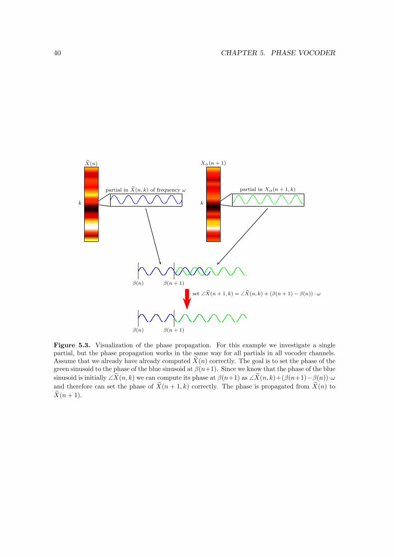
40 CHAPTER 5. PHASE VOCODER
X(n) Xα(n+ 1)
k k
partial in X(n, k) of frequency ω partial in Xα(n+ 1, k)
β(n) β(n+ 1)
β(n) β(n+ 1)
set ∠X(n+ 1, k) = ∠X(n, k) + (β(n+ 1)− β(n)) · ω
Figure 5.3. Visualization of the phase propagation. For this example we investigate a singlepartial, but the phase propagation works in the same way for all partials in all vocoder channels.Assume that we already have already computed X(n) correctly. The goal is to set the phase of thegreen sinusoid to the phase of the blue sinusoid at β(n+1). Since we know that the phase of the blue
sinusoid is initially ∠X(n, k) we can compute its phase at β(n+1) as ∠X(n, k)+(β(n+1)−β(n))·ω
and therefore can set the phase of X(n + 1, k) correctly. The phase is propagated from X(n) to
X(n+ 1).

5.4. MODIFICATIONS FOR A SIMPLE IMPLEMENTATION 41
the magnitude spectrum |X(2)| = |Xα(2)|. To compute ∠X(2) we can proceed exactly asmentioned above for every single vocoder channel k. In this case the points n and m areβ(1) and β(2). This technique is called phase propagation since the phases of a Fourierspectrum in a sequence of Fourier spectra are propagated to the next spectrum in thesequence. The process is visualized in Figure 5.3.
The problem is that we do not know the frequencies of all the partials in the vocoderchannels exactly. Let Ωk = 2·π·k
N be the center frequency of the kth vocoder channel. Apartial lying in a phase vocoder channel with center frequency Ωk not necessarily has thefrequency Ωk by itself. It just has a frequency that is closer to Ωk as to any other centerfrequency of the remaining vocoder channels. We therefore have to estimate the exactfrequencies of all the partials first. To this end we compute the so called heterodyned phase
increment of vocoder channel k at analysis instance α(n) which is denoted by ∆φα(n)k .
∆φα(n)k = ∠Xα(n, k)− ∠Xα(n− 1, k)− (α(n)− α(n− 1)) · Ωk . (5.10)
The term ∠Xα(n, k)−∠Xα(n−1, k) describes the phase increment from analysis instanceα(n− 1) to α(n) that is actually present in the Fourier spectra. The term (α(n)− α(n−1)) · Ωk on the other hand describes the expected phase increment in case the partial invocoder channel k had exactly frequency Ωk. The heterodyned phase increment thereforedescribes the small deviation of the computed phase increment from the phase incrementthat a partial with frequency exactly Ωk would have had. Note that we have to shift the
heterodyned phase increment ∆φα(n)k to the range [−π, π) such that it is a valid phase.
For the sake of simplicity we will denote the shifted version by ∆φk.
From ∆φk we now can compute the actual frequency of the partial that lies in vocoderchannel k at analysis instance α(n). This frequency is called the instantaneous frequencyof the partial at position α(n) and is denoted by ωk(α(n)). Note that dividing a phase ϕby some distance d yields the frequency of the sinusoidal wave that has phase ϕ at d.
ωk(α(n)) = Ωk +∆φk
α(n)− α(n− 1). (5.11)
Finally having estimated the exact frequencies we can apply the phase propagation by
∠X(n, k) = ∠X(n− 1, k) + (β(n)− β(n− 1)) · ωk(α(n)) . (5.12)
5.4 Modifications for a simple implementation
In implementations of the Phase Vocoder it is often convenient to keep the rather complexphase propagation as simple as possible. To this end we can modify the pipeline describedin 5.2 a little bit. Instead of achieving the time-scale modification by spacing the analysisinstances of the STFT differently from the synthesis instances we can also construct acompletely new sequence of Fourier spectra for the output signal from the STFT of theinput signal. The core idea of the new approach, and the reason why the phase propagation

42 CHAPTER 5. PHASE VOCODER
(a)
xα(1) α(2) α(3) α(4) α(5)
Xα Xα(1) Xα(2) Xα(3) Xα(4) Xα(5)
X X(1) X(2) X(3) X(4) X(5)
yβ(1) β(2) β(3) β(4) β(5)
(b)
xα(1) α(2) α(3)
Xα Xα(1) Xα(2) Xα(3)
X X(1) X(2) X(3) X(4) X(5)
yβ(1) β(2) β(3) β(4) β(5)
STFT using α
Respacing and phase adaption
iSTFT using β
STFT using α
Interpolation and phase adaption
iSTFT using β
hop
hop
Figure 5.4. (a) Schematic overview of the standard Phase Vocoder. Note that the vectors α andβ are of the same length. (b) Schematic overview of the modified Phase Vocoder for a simplerimplementation. In opposite to the standard Phase Vocoder the Fourier Spectra for the outputsignal y are not directly computed from the input signal x but interpolated from some spectra thatwere computed at equidistant analysis instances α. Note that therefore the length of the vector ofanalysis instances α is unequal to the length of the vector of synthesis instances β. Note furtherthat all analysis instance and synthesis instances are spaced apart by the same distance hop

5.4. MODIFICATIONS FOR A SIMPLE IMPLEMENTATION 43
becomes simple in the end, is to have equidistant analysis and synthesis instances, allspaced apart by a constant value. This value is called the hop factor and is denotedby hop. Note that therefore the vectors α and β do not need to be of the same lengthany more. In fact whenever the duration of a time-scale modified signal differs fromthe duration of the initial signal their length will also differ. Figure 5.4 visualizes thedifferences between the two Phase Vocoder approaches.
For a given input signal x and a time-stretch function τ we can define
(i) length(α) = ⌈ length(x)hop⌉
(ii) α(1) = 1(iii) α(n) = α(n− 1) + hop for n ∈ [2 : length(α)]
(5.13)
(i) length(β) = ⌈ length(y)hop⌉
(ii) β(1) = 1(iii) β(n) = β(n− 1) + hop for n ∈ [2 : length(β)]
(5.14)
Applying the STFT to the input signal x at analysis instances α yields Xα. Our goalis now to construct from Xα a sequence of Fourier spectra X of length length(β) suchthat when applying the inverse Fourier Transform to X using synthesis instances β weget the desired output signal. We start by first constructing a sequence of Fourier spectraX that has the same magnitude spectrum as X such that it holds that |X| = |X|. Letfxα : [1 : length(x)]→ CN be a function defined as follows.
fxα(t) =t−α(i)
α(i+1)−α(i) ·Xα(i) +α(i+1)−t
α(i+1)−α(i) ·Xα(i+ 1) for α(i) ≤ t ≤ α(i+ 1) . (5.15)
The function fxα assigns to every sample position in x a Fourier spectrum that was com-puted by linear interpolation between the Fourier spectra of x at analysis instances α. Wetherefore can compute
X(n) = fxα(τ−1(β(n))) . (5.16)
The internal encoding of the time-stretch function τ therefore does not lie in the vectorsof analysis and synthesis instances anymore, but in the sequence of Fourier Spectra itself.
Having computed X and knowing that |X| = |X| we now have to take care of the phases∠X. This is again done using the phase propagation technique. Recall that to computethe phase propagation we have to know the exact frequencies of all the partials lyingin the vocoder channels. To compute these exact frequencies we can use the phases oftwo successive Fourier spectra. Unfortunately we can not assume the phases of X to bemeaningful since X was computed by linear interpolation. The only source of reliablephase information is the sequence of Fourier spectra Xα. We therefore assume that allFourier spectra in X that were computed by linear interpolation between Xα(n− 1) andXα(n) have those exact frequencies that can be computed using Xα(n−1) and Xα(n). To

44 CHAPTER 5. PHASE VOCODER
be able to compute those exact frequencies we need to be able to access these two spectragiven the index of a synthesis instance in β. Note that the term
gm = α
(⌈τ−1(β(m))
hop
⌉)(5.17)
yields the index i in α such that α(i) is the biggest entry in α that is smaller than τ−1(β(m))since the difference between two analysis or synthesis instances is by construction alwaysconstantly hop. Furthermore gm + 1 is the index of the smallest entry in α that is largerthan τ−1(β(m)). Therefore we can define
X1(m) = Xα(gm) (5.18)
andX2(m) = Xα(gm + 1) . (5.19)
X1(m) and X2(m) are exactly the two spectra that were used to interpolate X(m).
Finally we can compute the phase propagation as
∠X(n, k) = ∠X(n− 1, k) + hop · ωk(α(n)) (5.12)
= ∠X(n− 1, k) + hop · (Ωk +∆φkhop
) (5.11)
= ∠X(n− 1, k) + hop · Ωk +∆φk= ∠X(n− 1, k) + hop · Ωk
+(∠X2(n, k)− ∠X1(n, k)− hop · Ωk) (5.10)
= ∠X(n− 1, k) + (∠X1(n, k)− ∠X2(n, k))
In other words, whenever we want to calculate the phase ∠X(n) for a magnitude spectrum|X(n)| that was constructing by linear interpolation between two Fourier spectra X1(n)and X2(n) we simply have to add the phase differences ∠X2(n) − ∠X1(n) to the knownphases ∠X(n − 1) (where ∠X(1) = Xα(1),). Note that in the computations above weargued about a single vocoder channel. But since the computations are the same for everyvocoder channel we can do the computations on the whole spectra directly.
We get the time-scale modified output signal y by applying the iSTFT to X using theanalysis instances β. The modified pipeline is visualized in Figure 5.5.
5.5 Artifacts
When listening to audio signals produced by the Phase Vocoder they often sound like ifthe content of the original signal was played in some distance. Percussive elements in thesignal sound hollow and also non percussive parts sound phasy. These artifacts occur notonly when applying large time-stretch factors but immediately when time-scale modifyingthe signal only slightly. The cause of these artifacts lies in the destruction of the verticalphase coherence of the signal. By design, the Phase Vocoder ensures horizontal phase

5.5. ARTIFACTS 45
STFT using synthesis instances α
Interpolation of Spectra
Phase adjustment
iSTFT using synthesis instances β
x
Xα
X
X
y
Figure 5.5. The pipeline of the modified Phase Vocoder. In this example the Phase Vocoder isapplied with a time-stretch factor of 2. Note that the length of X is twice the length of Xα.
coherence, meaning that over the duration of the signal the phases in a vocoder channelare adapted such that there occur no phase jumps in this particular vocoder channel. Butfor the overall sound of the signal also the relations of the phases in the several vocoderchannels at a given point in time are important. These relations are referred to as verticalphase coherence and they are not maintained by the Phase Vocoder. Figures 5.6 andFigure 5.7 show examples how the loss of vertical phase coherence affects an audio signal.

46 CHAPTER 5. PHASE VOCODER
−1
0
1
−1
0
1
−1
0
1
−1
0
1
−1
0
1
−1
0
1
−1
0
1
−1
0
1
f1
f2
f3
fsum
f1
f2
f3
fsum
(a) (b)
Figure 5.6. (a) The three partials f1, f2 and f3 form the signal fsum. The signal fsum has aclear peak structure. (b) The frequencies of the partials f1, f2 and f3 are the same as in (a), butthe phases are slightly modified. The signal fsum lost its peak structure because of the destroyedvertical phase coherence.
0 1 2 3 4
0 1 2 3 4
Figure 5.7. The audio signal of drum beat and its time-scale modified version produced with thePhase Vocoder. The constant time-stretch factor used in this example is 1.01. One can observe thatthe amplitude of the peaks decreased in the time-scale modified version. Note that the amplitude ofthe first beats were only slightly decreased. This is due to the fact that we initialized X(1) = Xα(1)and the deviation from the initial vertical phase coherence is therefore smaller at the beginning ofthe signal.

Chapter 6
Transient Preserving WSOLA
As noted in Section 4.3 stuttering artifacts at transients are a significant cause for audiosignal quality degradation in WSOLA. A method to prevent this kind of degradation is theso called transient preservation. The core idea is to suspend the time-scale modification attransient positions in the audio signal. To compensate for these suspensions the remainingparts of the signal are stretched with a slightly different time-stretch factor. This can bedone by manipulations of the time-stretch function τ . In this chapter we first introducea novel, simple and effective way of representing time-stretch functions in Section 6.1.Afterwards we will discuss the transient preservation process in detail: We start withsome basic transient detection in Section 6.2. Knowing the positions of the transientsin an audio signal we can proceed with the transient preservation by manipulating thetime-stretch function. The process is explained in detail in Section 6.3. Afterwards wewill investigate the limits of transient preservation in Section 6.4.
6.1 Anchor Points
In practical applications it is necessary to have a simple and practical representation ofthe time-stretch function τ as an input for the WSOLA algorithm. We therefore representit by a set of so called anchor points. An anchor point is a pair of two points in timewhere the first entry specifies a point in time in the input audio signal and the secondentry specifies where this point in time should be mapped to in the output audio signal.Between two anchor points the audio signal is modified in a linear fashion. Using anchorpoints is a simple way of expressing piecewise linear time-stretch functions which aresufficient for most applications. For example in the context of the Connector wherewe want to rearrange the beat positions of an audio signal, we have exactly one anchorpoint per beat. The first entry of the anchor point is set to the time of the beat in theinput audio signal and the second entry to the time where the beat should be placed. Anexample can be seen in Figure 6.1.
In fact, also constant time-stretch factors are realized using anchor points. In case ourWSOLA implementation receives a global time-stretch factor t as an input along with anaudio signal x, the implementation just introduces two anchor points: one to synchronize
47

48 CHAPTER 6. TRANSIENT PRESERVING WSOLA
0 1 2 3 4 5 6 7 8−1
0
1
0 1 2 3 4 5 6 7 80123456789
1011
0 1 2 3 4 5 6 7 8 9 10 11−1
0
1
x(n)
y(n)
Anchor points
Figure 6.1. An audio signal x and its time-scale modified version y (time is given in seconds).The non-linear time-scale modification was specified using a set of anchor points. For each beatin x (indicated by red bars) there exists an anchor point that specifies the point in time wherethis beat should be mapped to in the output. Note that the red bars in y mark exactly the beatpositions again.
the beginnings of input and output (this is the anchor point (1, 1) that maps sampleposition 1 in the input to sample position 1 in the output) and one to synchronize theendings (which is (length(x), t · length(x)) since the output should have t times the lengthof the input).
To compute the input position vector σ we interpolate τ from the set of anchor pointsby discrete linear interpolation (recall from Chapter 4 that σ is computed by σ(n) =τ−1(γ(n)). This was defined in Equation 4.2). Note that in principle the anchor pointsform exactly a discretized time-stretch function according to Definition 3.4. To computeσ we then can use the inverted interpolated time-stretch function accoring to Definition3.6.
6.2 Transient Detection
Not every transient in an audio signal causes a stuttering artifact when time-scale ma-nipulating the signal with WSOLA. These artifacts are for example rarely audible whentime-scale modifying a recording of a violin. On the other hand they are almost alwayspresent when stretching the recording of a drum. To find the transients that produce theundesired stuttering artifacts in WSOLA it is therefore necessary to first describe the classof artifact causing transients.
According to our experience the most perceivable stuttering artifacts occur at points inthe signal where some source produces a short, noise like burst of energy. These burstsare then audible several times in the time-scale modified signal what causes the stutteringsound. Sound sources which frequently produce such artifacts are for example drum or

6.2. TRANSIENT DETECTION 49
cymbal hits but also strong onsets of instruments that have a percussive component like apiano. In general we can say that we are looking for strong note onsets of both percussiveand non-percussive instruments. A note onset is the point in an audio signal where theperception of the note starts and it is commonly marks the beginning of a transient. SeeFigure 6.2 for an example. Unfortunately the task of detecting onsets in an audio signal isby far not trivial. A lot of work has been done in this field (for example [20, 2, 5, 4, 27, 7]),but the task of finding all note onsets in an arbitrary audio signal is not solved yet. Thereason for this is that a perfect onset detection algorithm should be able to detect even thesoftest onsets like for example those of softly played violins. This is extremely difficult.Fortunately we do not need a perfect onset detection algorithm. We are only interestedin onsets that are well perceivable as such since stuttering artifacts are not likely to occurat soft note onsets. The task of finding this kind of note onsets is much simpler. We arelooking for massive bursts of energy in the frequency content of the signal. These canbe found by looking for peaks in the sum of the magnitudes of all frequency bands. Wealso feel that the high frequency bands contribute more to noticeable transients than thelow frequency bands and therefore weight the high frequency content more than the lowfrequencies. To this end we combine two standard techniques and apply them to the audiosignal. Let x be the input audio signal. We first introduce the high frequency content ofx [4]
HFCx(n) =
N/2∑
k=2
k · |Xα(n)|2 , (6.1)
where α is a vector of equidistant analysis instances in x of length M , n ∈ [1 : M ] andXα is the Short Time Fourier Transform of x according to the definitions introduced inChapter 5. The high frequency content is a function that describes the instantaneousenergy of the signal at a given point in time while the energy in high frequency bands isweighted more than the energy in low frequency bands.
A standard technique to find bursts of energy in an audio signal is the so called spectraldifference [2]. It is defined by
SDx(n) =
N/2∑
k=1
(|Xα(n)| − |Xα(n− 1)|)2 . (6.2)
In principle SDx(n) computes a simple derivative of every single frequency band and sumsup the values to get a one dimensional function. A burst in energy in the signal means amassive increase of the values in many frequency bands. Therefore the derivative is highin many frequency bands at the same time and SDx(n) yields high values at this point.
Finally we combine the high frequency content with the spectral difference by weight-ing the frequency bands in the spectral difference similar to the high frequency content.We applied a logarithmic compression function to the Fourier spectra to account for the

50 CHAPTER 6. TRANSIENT PRESERVING WSOLA
onset
transient
Figure 6.2. Note onset and transient according to [2].
logarithmic perception of loudness of the human ear.
Dx(n) =
N/2∑
k=1
k · (| log(1 + C ·Xα(n))| − | log(1 + C ·Xα(n− 1)|) (6.3)
with
Dx(1) =
N/2∑
k=1
k · | log(1 + C ·Xα(1))| . (6.4)
We set C = 100 in our experiments. In the function Dx we already have peaks at allthe interesting transient positions in the input signal, but we also have a lot of noise andnegative values that we do not need. The noise comes from smaller energy variations thatdo not originate from transients. The negative values indicate abrupt drops of the energy.Since we want to focus on note onsets, sudden drops of energy are not of interest to us.We therefore introduce a threshold function λ. Let GsDx be a version of Dx smoothed witha Hann-window of a length that is equivalent to s seconds in x. Furthermore, let v be thevalue of the global maximum of Dx. We define λ by
λ(n) = κlocal ·GsDx(n) + κglobal · v , (6.5)
where κlocal, κglobal ∈ R are variables to control the influence of the two parts. Thethreshold function λ is therefore a combination of a local averageGsDx and a global absolutethreshold κ · v. We then compute
Tx(n) = max(0, Dx(n)− λ(n)) . (6.6)
We call the function Tx a novelty curve of the signal x. Figure 6.3 shows the audio signalof a musical scale played on a piano together with its novelty curve.
It is important to notice that our transient detection method is not meant to be a state ofthe art onset detector. Modern onset detectors tend to be very sensitive to the input audiosignal and often yield false positives. Furthermore, they are often capable of detecting

6.2. TRANSIENT DETECTION 51
0 1 2 3 4 5 6 7 8
0 1 2 3 4 5 6 7 8
0 1 2 3 4 5 6 7 8
0 1 2 3 4 5 6 7 8
0 1 2 3 4 5 6 7 8
(a)
(b)
(c)
(d)
(e)
Figure 6.3. (a) The waveform of an audio signal x of a musical scale played on a piano. (b) TheShort Time Fourier Transform Xα for a vector of equidistant analysis instances α. (c) The ShortTime Fourier Transform from (b) with weighted frequency bands and logarithmic scaling applied.(d) The function Dx. The red line indicates the threshold that will be applied. (e) The noveltycurve Tx.

52 CHAPTER 6. TRANSIENT PRESERVING WSOLA
our approach Grosche et al.
Filename Precision Recall Precision Recallcello1 0.333 0.164 0.730 0.885clarinet1 0.200 0.114 0.061 0.086classic2 0.429 0.079 0.388 0.868classic3 0.000 0.000 0.023 0.500distguit1 0.857 0.316 0.875 0.737guitar2 0.880 0.611 0.842 0.889guitar3 0.976 0.732 0.966 1.000jazz2 0.692 0.383 0.821 0.681jazz3 0.838 0.585 0.975 0.736piano1 1.000 0.632 0.950 1.000pop1 0.941 0.593 0.719 0.852rock1 0.875 0.237 0.935 0.729sax1 0.714 0.556 0.136 0.333synthbass1 0.846 0.478 0.905 0.826techno2 0.972 0.625 0.940 0.839trumpet1 0.538 0.125 0.959 0.839violin2 0.750 0.288 0.771 0.877Average 0.697 0.383 0.706 0.746
Table 6.1. Precision/Recall Results. An onset was counted as detected correctly if it lied in atolerance region of 50 ms around the reference onset. Database and reference annotations takenfrom [29].
softer onsets which are not of interest to us since such onsets do not cause stutteringartifacts in WSOLA. Detecting too many erroneous transients (either positions where noonset takes place or the present onset is not artifact causing) can even degenerate theoutput audio quality. The transient preservation is realized by a manipulation of thetime-stretch function (see Section 6.3). A huge amount of erroneously detected transientstherefore leads to a degeneration of the time-stretch function or even to a suppression ofthe correctly detected transients.
We tested our transient detection method on an onset-annotated dataset of 17 short mu-sical excerpts [29] together with a state of the art onset detection algorithm developed byGrosche et al. [20]. A detected onset was classified as correctly detected, or true positive(TP), in case it was located in a 50 ms tolerance region around a reference onset. Other-wise it was classified as false positive (FP). In case no onset was detected for a referenceonset this was considered a false negative (FN). We then computed precision and recallas follows.
Precision =TP
TP + FP, Recall =
TP
TP + FN. (6.7)
The results can be seen in Table 6.1. It shows that the precision of our method is onlyslightly worse than the precision of the state of the art method. The recall on the otherhand is of course lower. Nevertheless, listening tests revealed that most of the missedtransients were not artifact causing. Figure 6.4 shows the detected onsets of both methodsfor an example excerpt.

6.3. TRANSIENT PRESERVATION 53
0 2 4 6 8 10 12 14
Reference
0 2 4 6 8 10 12 14
Our approach
0 2 4 6 8 10 12 14
Grosche et al.
Figure 6.4. Onset detection results for the musical excerpt pop1 from our dataset. The time isgiven in seconds. Vertical lines indicate the onset positions. In the reference we indicated onsetsthat cause stuttering artifacts by red bars and onsets that are unproblematic when time-scalemodifying with WSOLA by blue bars. The classification was done by listening tests. The excerptwas time-scale modified using WSOLA with a global time-stretch factor of 2. Afterwards theartifact causing transient were identified manually. One can see that our approach is capable ofdetecting a large amount of artifact causing transients and at the same time yield only few falsepositives.
6.3 Transient Preservation
Knowing the positions of the transients in the input audio signal x we now can preservethese transients when time-scale modifying x. Recall that given to our WSOLA algorithmis the input signal x together with a set of anchor points that describe the intended time-stretch function τ . The core idea of the transient preservation is to modify the set of anchorpoints, and therefore the time-stretch function τ , such that at transient positions we havea local time-stretch factor of 1, i.e. no time-scale modification. Let p ∈ [1 : length(x)] bethe position of a transient in the input signal. To preserve this transient we insert two newanchor points (n1,m1) and (n2,m2) into the set of anchor points. For these new anchorpoints it holds that
(i) n1 = p− ǫ1(ii) m1 = τ(p)− ǫ1(iii) n2 = p+ ǫ2(iv) m2 = τ(p) + ǫ2(v) n2−n1
m2−m1= 1
(6.8)
with ǫ1, ǫ2 ∈ N (see Figure 6.5). We call the interval [n1 : n2] the transient window anddenote it by Ξ. Intuitively Ξ marks an area around the transient in the input signal. Byusing this technique we can manipulate the time-stretch factor locally but at the same time

54 CHAPTER 6. TRANSIENT PRESERVING WSOLA
(p, τ(p)) (p, τ(p))
(n1,m1)
(n2,m2)
detected transient p detected transient p
ǫ1 ǫ2
ǫ1
ǫ2
(a) (b)
Figure 6.5. (a) A segment of a time-stretch function τ . The anchor points are indicated by redcircles. The position p marks the point in the input audio where a transient was detected. (b) Topreserve the transient at position p two new anchor points (n1,m1) and (n2,m2) are introducedto create a short segment with local time-stretch factor 1 where n1 = p − ǫ1, m1 = τ(p) − ǫ1,n2 = p+ ǫ2 and m2 = τ(p) + ǫ2.
keeping the global time-stretch function intact. Unfortunately, since WSOLA works withwindows of fixed length, it can not guarantee that time-relations specified by the set ofanchor points are realized exactly. Just because there are two anchor points that indicatea very small time-scale modification free segment does not mean that there will actuallybe a time-scale modification free segment in the output signal of WSOLA. To ensure theexistence of such a segment around the transient we have to take care that the two newanchor points are not spaced too close to each other. For the sake of simplicity let us firstconsider the basic OLA scenario neglecting the existence of the window position tolerance∆max. In this scenario we have to ensure that there are at least ⌈ 1
1−o⌉ input windowpositions placed in the interval Ξ where o is the overlap factor of the OLA algorithm. Thisis because in a signal that was constructed by adding up a sequence of windowed audiosegments overlapping by a constant factor o, there are always at most ⌈ 1
1−o⌉ windowedaudio segments that contribute to a given point in the signal. Furthermore, we know thatthe windows that will be placed in the interval Ξ will all be equidistantly spaced apartby the standard window offset ηwo . This is because the local slope of the time-stretchfunction τ is exactly 1 in the interval Ξ by design of the two new inserted anchor points.A slope of 1 indicates that the windows in the input are spaced exactly as the windowsin the output, and the windows in the output are all equidistantly spaced apart by ηwoby design of OLA. Summarizing we have to ensure that there are at least ⌈ 1
1−o⌉ inputwindow positions spaced apart by ηwo lying in the interval Ξ to guarantee the existenceof an interval I ⊆ Ξ in the input signal such that this interval is not time-scale modifiedwhen applying OLA. See Figure 6.6 for an example. Note that since the exact positions ofthe input windows are not only determined by the time-stretch function τ but also by thefixed output position vector γ, the exact position of I in Ξ can not be precisely specifiedupfront. From these requirements we now can compute the minimal distance between n1and n2 and therefore the size of the transient window Ξ.
length(Ξ) = n2 − n1 ≥
⌈1
1− o
⌉· ηwo ≥
1
1− o· ηwo =
1
1− o· (1− o) · wℓ = wℓ . (6.9)

6.3. TRANSIENT PRESERVATION 55
0
1
detected transient
n1 n2
Figure 6.6. In this example we set o = 12 . We therefore need at least 1
1− 1
2
= 2 input window
positions spaced apart by ηwo = (1− 12 ) ·wl =
12 ·wl in the interval Ξ = [n1 : n2] around the detected
transient such that there exists an interval I ⊆ Ξ (blue area) that is not time-scale modified in theoutput.
0
1
detected transient
n1 n2
Figure 6.7. An example where an interval I ⊆ Ξ exists but the detected transient does not lie inI (blue area) and is therefore not preserved.
Equation 6.9 yields a lower bound on the size of the interval Ξ to ensure the existence ofI. Furthermore, the length of the time-scale modification free interval I can be assessedby
length(I) ≥
(⌊n2 − n1ηwo
⌋− 1
)· ηwo (6.10)
since it holds that N windows that are all equidistantly spaced apart byM yield a segmentof length (N − 1) ·M to which only these N windows contribute to. Further, the term⌊ LM ⌋ describes the minimal number of points that lie in a segment of length L in case thepoints are equidistantly spaced apart by M .
At this point we know how large we have to choose Ξ to guarantee the existence of I.Furthermore, we can even estimate the size of I. But we have another problem. Eventhough we can guarantee the existence of the interval I, we do not know its exact positionin the interval Ξ. It is therefore possible that p /∈ I for p being the position of the detectedtransient. See Figure 6.7 for an example. To ensure that a detected transient is always

56 CHAPTER 6. TRANSIENT PRESERVING WSOLA
preserved we have to take care that the time-scale modification free interval I is largeenough and will definitely include p. Therefore we will now construct constraints suchthat fulfilling these constraints guarantees the preservation of the transient.
Recall at this point that we only discussed a transient preservation for the basic OLAtechnique so far. In WSOLA all window positions may shift by the window positiontolerance ∆max. Therefore the whole time-scale modification free segment I may shift bythe same amount. In WSOLA, the subset relationship I ⊆ Ξ = [n1 : n2] therefore has tobe replaced by I ⊂ [n1 −∆max : n2 +∆max]. Note that all other assessments stay valid.To ensure that a detected transient at position p lies in the interval I it therefore has tohold that
p ∈ Q = [n2 +∆max − length(I) : n1 −∆max + length(I)] . (6.11)
The interval Q includes all points q such that q ∈ I is independent of the position of I in[n1 −∆max : n2 +∆max]. We therefore can conclude
p ∈ Q = [n2 +∆max − length(I) : n1 −∆max + length(I)]⇔ p ∈ [p+ ǫ2 +∆max − length(I) : p− ǫ1 −∆max+ length(I)]⇔ p ≥ p+ ǫ2 +∆max − length(I) and p ≤ p− ǫ1 −∆max + length(I)⇔ ǫ2 ≤ length(I)−∆max and ǫ1 ≤ length(I)−∆max
(6.12)
We therefore get the following set of constraints to guarantee the preservation of thetransient
(i) length(Ξ) = length([n1 : n2]) = ǫ1 + ǫ2 ≥ wℓ (6.8), (6.9)(ii) ǫ1 ≤ length(I)−∆max (6.12)(iii) ǫ2 ≤ length(I)−∆max (6.12)
(6.13)
But since we do not know the exact size of I we use the lower bound on I from Equation6.10 to strengthen the constraints.
(i) length(Ξ) = length([n1 : n2]) = ǫ1 + ǫ2 ≥ wℓ (6.8), (6.9)
(ii) ǫ1 ≤ (⌊ length(Ξ)ηwo⌋ − 1) · ηwo −∆max (6.10)
(iii) ǫ2 ≤ (⌊ length(Ξ)ηwo⌋ − 1) · ηwo −∆max (6.10)
(6.14)
6.4 Limitations of the Transient Preservation
To ensure that the segment that is defined by the two new anchor points (n1,m1) and(n2,m2) is indeed time-scale modification free it makes sense to delete any other anchorpoints (n,m) with n1 < n < n2 or m1 < m < m2. This can lead to problems in casetwo transients are close together and an anchor point, that were inserted to preserve theother transient, is deleted. We therefore proceed in an iterative fashion and choose thenext transient that should be preserved by picking the highest peak in the novelty curve

6.4. LIMITATIONS OF THE TRANSIENT PRESERVATION 57
Tx. After having modified the set of anchor points to preserve the just found transient,the indicating peak is removed from the novelty curve and the next highest peak is picked.This process makes sense since the hight of a peak correlates directly to the energy, andtherefore to the loudness of the causing transient and of course stuttering artifacts at aloud transient are more noticeable than the artifacts at a rather unobtrusive transient. Tosave anchor points that were inserted to preserve a transient from being deleted duringthe process we separate the set of anchor points in two parts. Let A be the set of anchorpoints. We define
A = Adeletable ∪Anondeletable , (6.15)
where the sets Adeletable and Anondeletable are disjoint. At the beginning of the transientpreservation process we define Adeletable to be the set of all anchor points that describeτ and Anondeletable = ∅. Whenever we now want to insert new anchor points (n1,m1)and (n2,m2) into the set of anchor points and there exists an anchor point (n′,m′) ∈Anondeletable with n1 < n′ < n2 or m1 < m′ < m2 the current transient is skippedand we proceed with the next transient. Otherwise the new anchor points are added toAnondeletable and we have Anondeletable = Anondeletable ∪ (n1,m1), (n2,m2). In case thereexists an anchor point (n′′,m′′) ∈ Adeletable with n1 < n′′ < n2 or m1 < m′′ < m2 thisanchor point is deleted and we have Adeletable = Adeletable\(n
′′,m′′). This prevents thedegeneration of the time-stretch function τ and ensures that the strongest transients arepreferred during the process. Figure 6.8 shows an example. The procedure is summerizedin Algorithm 4.
Using this technique ensures that the stronger transients are preferred over weaker tran-sients. But at the same time it implies limitations on the number of transients that canbe preserved in an audio signal of a certain length. More precisely, for a given local time-stretch factor ψ and a fixed length of transient windows Ξℓ there exists a minimal distanceδmin between two transient positions such that both transients can be preserved. Thisdistance can be computed as follows
δmin =
Ξℓ + 1 if ψ ≥ 11ψ · Ξℓ + 1 if ψ < 1
(6.16)
The reason for this is the following: Assume we have two transients at positions p′ and p′′
in our input signal and assume further that w.l.o.g. p′ < p′′. To preserve those transientswe want to insert new anchor points (n′1,m
′1), (n
′2,m
′2) for p′ and (n′′1,m
′′1), (n
′′2,m
′′2) for
p′′ into the set of anchor points such that it holds that
(i) n′1 = p′ − ǫ1(ii) m′
1 = τ(p′)− ǫ1(iii) n′2 = p′ + ǫ2(iv) m′
2 = τ(p′) + ǫ2
(v)n′
2−n′
1m′
2−m′
1= 1
(6.17)
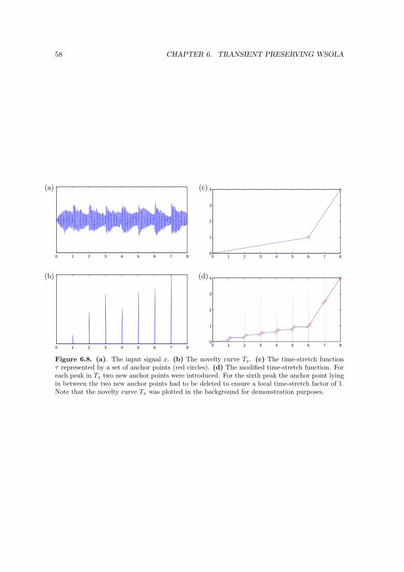
58 CHAPTER 6. TRANSIENT PRESERVING WSOLA
0 1 2 3 4 5 6 7 8
0 1 2 3 4 5 6 7 8
0 1 2 3 4 5 6 7 80
1
2
3
4
0 1 2 3 4 5 6 7 80
1
2
3
4
(a)
(b)
(c)
(d)
Figure 6.8. (a). The input signal x. (b) The novelty curve Tx. (c) The time-stretch functionτ represented by a set of anchor points (red circles). (d) The modified time-stretch function. Foreach peak in Tx two new anchor points were introduced. For the sixth peak the anchor point lyingin between the two new anchor points had to be deleted to ensure a local time-stretch factor of 1.Note that the novelty curve Tx was plotted in the background for demonstration purposes.
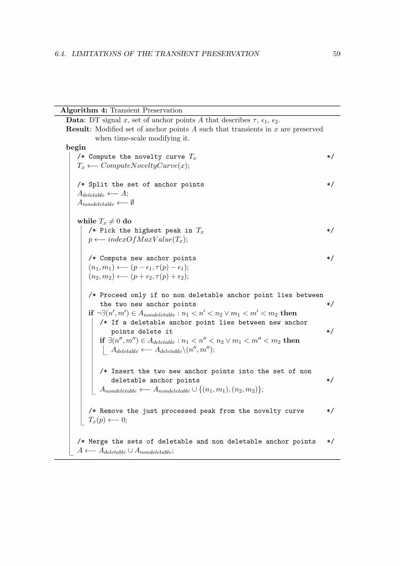
6.4. LIMITATIONS OF THE TRANSIENT PRESERVATION 59
Algorithm 4: Transient Preservation
Data: DT signal x, set of anchor points A that describes τ , ǫ1, ǫ2.Result: Modified set of anchor points A such that transients in x are preserved
when time-scale modifying it.begin
/* Compute the novelty curve Tx */
Tx ←− ComputeNoveltyCurve(x);
/* Split the set of anchor points */
Adeletable ←− A;Anondeletable ←− ∅
while Tx 6= 0 do/* Pick the highest peak in Tx */
p←− indexOfMaxV alue(Tx);
/* Compute new anchor points */
(n1,m1)←− (p− ǫ1, τ(p)− ǫ1);(n2,m2)←− (p+ ǫ2, τ(p) + ǫ2);
/* Proceed only if no non deletable anchor point lies between
the two new anchor points */
if ¬∃(n′,m′) ∈ Anondeletable : n1 < n′ < n2 ∨m1 < m′ < m2 then/* If a deletable anchor point lies between new anchor
points delete it */
if ∃(n′′,m′′) ∈ Adeletable : n1 < n′′ < n2 ∨m1 < m′′ < m2 thenAdeletable ←− Adeletable\(n
′′,m′′);
/* Insert the two new anchor points into the set of non
deletable anchor points */
Anondeletable ←− Anondeletable ∪ (n1,m1), (n2,m2);
/* Remove the just processed peak from the novelty curve */
Tx(p)←− 0;
/* Merge the sets of deletable and non deletable anchor points */
A←− Adeletable ∪Anondeletable;

60 CHAPTER 6. TRANSIENT PRESERVING WSOLA
p′ p′′
δmin = Ξℓ + 1
(n′
1,m′
1)
(n′
2,m′
2)
(n′′
1 ,m′′
1 )
(n′′
2 ,m′′
2 )
Figure 6.9. The minimal distance δmin between transient positions p′ and p′′ such that bothtransients can be preserved in case the local time-stretch factor ψ is greater one. The original time-stretch function τ is indicated by the straight blue line while the time-stretch function resultingfrom the insertion of the new anchor points is indicated by the dashed blue line.
and accordingly for n′′1, m′′1, n
′′2, m
′′2 and p′′. To circumvent that one of the two transients
is skipped during the transient preservation process it has to hold that
(i) n′2 < n′′1 ⇔ p′ + ǫ2 < p′′ − ǫ1 ⇔ Ξℓ < p′′ − p′
(ii) m′2 < m′′
1 ⇔ τ(p′) + ǫ2 < τ(p′′)− ǫ1 ⇔ Ξℓ < τ(p′′)− τ(p′)(6.18)
Note that the difference τ(p′′) − τ(p′) can be computed by ψ · (p′′ − p′) since we assumea constant time-stretch factor and the time stretch function τ is therefore linear. In casethe local time-stretch factor ψ is greater or equal to one we therefore automatically fulfillthe second requirement in Equation 6.18 when fulfilling the first, and the first requirementis fulfilled when p′′ − p′ ≥ Ξℓ + 1. In contrary, in case the local time-stretch factor ψis smaller than one, we fulfill the first requirement automatically whenever fulfilling thesecond which is fulfilled when p′′ − p′ ≥ 1
ψ · Ξℓ + 1. Examples can be seen in Figure 6.9and Figure 6.10.

6.4. LIMITATIONS OF THE TRANSIENT PRESERVATION 61
p′ p′′
δmin = 1ψ
· Ξℓ + 1
(n′
1,m′
1)
(n′
2,m′
2) (n′′
1 ,m′′
1 )
(n′′
2 ,m′′
2 )
Figure 6.10. The minimal distance δmin between transient positions p′ and p′′ such that bothtransients can be preserved in case the local time-stretch factor ψ is smaller one. The original time-stretch function τ is indicated by the straight blue line while the time-stretch function resultingfrom the insertion of the new anchor points is indicated by the dashed blue line.

62 CHAPTER 6. TRANSIENT PRESERVING WSOLA

Chapter 7
Listening Test
To gain further insights into the quality of WSOLA and the transient preservation inWSOLA we performed a listening test. While performing this test we had the followingleading questions:
• How does WSOLA perform on an absolute scale? (In comparison to a perfect time-scale modification algorithm)
• How does WSOLA perform in comparison to other time-scale modification algo-rithms?
• How great is the effect of transient preservation in WSOLA?
In Section 7.1 we describe the dataset we performed the listening test on. The test setupis discussed in 7.2 and results are presented in 7.3.
7.1 Test Dataset
Our test dataset consists of 10 short sonified MIDI files, 4 extracted from the RWCdatabase [17] and 6 created by ourself (see Table 7.1). The files were chosen to covermusic of different styles, instrumentation, tempo and complexity. Furthermore, our self-created files were designed to have a repetitive structure such that possible artifacts occurseveral times and therefore can be better investigated by the listening test participants.All files were sonified using a state-of-the-art MIDI synthesizer.
7.2 Test Setup
From each sonified MIDI file in our test dataset we produced 4 time-scale modified versionswith a global time-stretch factor of two, using different time-scale modification algorithms:
63

64 CHAPTER 7. LISTENING TEST
Name content additional comment length
in
seconds
BASS1 Electric bass. 7.5
BONGO1 Regular beat played on Bongos. 6.2
DRUM1 Rock beat played on a standarddrum-set.
Open Hi-Hat and room reverb. 7.4
FLUTE1 Flute playing a simple melody. Strong natural tremolo at a long note. 6.9
GENRE1 Rock music. Playing instruments: flute,distorted electrical guitar, bass, drums
Polyphone music. Taken from RWCdatabase.
10.6
JAZZ1 Piano (left and right hand) Strong agogics. Taken from RWCdatabase.
13
OWN1 Electronic music. Bass and melodysynthesizer
The melody synthesizer produces sharp,noise-like onsets.
14.7
POP3 Pop music. Playing instruments: flute,piano, bass, steel guitar, quiet drums
Taken from RWC database. 11.1
POP4 Pop-Rock music. Playing instruments:distorted guitar, synthesizer, bass,drums.
Drums play fill-in at the end. Takenfrom RWC database.
9
VIOLIN1 Two violins. Strong vibrato. 10.5
Table 7.1. Short description of the used musical excerpts.
• A free MATLAB implementation of the Phase Vocoder1 similar to the implementa-tion explained in Section 5.4.
• The commercial MPEX4 algorithm2.
• Our implementation of WSOLA.
• Our implementation of the transient preserving WSOLA (TP-WSOLA).
The parameters and settings of the algorithms can be found in Table 7.2.
Since the onset detection itself was not part of the evaluation, we decided to eliminatepossible error sources by extracting all onset positions in the audio signals from the MIDIfiles and therefore skipping the possibly erroneous transient detection step in TP-WSOLA.Additional to the four time-scale modified versions we also produced a sonification of eachMIDI file that had half the tempo of the original version. Since time-scale modificationalgorithms are supposed to produce modifications of audio signals that sound as if therecorded musical piece was initially performed on a different tempo, the half-tempo MIDIsonification can be seen as the best possible result a time-scale modification algorithmcould produce. We decided to present this version along with the time-scale modifiedversions to the test participants to give them a reference on how the perfect result shouldsound. Nevertheless, the half-tempo MIDI reference was not specifically marked as such.
For all the excerpts from our test set the listening test proceeded as follows: The originalaudio recording along with the five time-scaled versions (four algorithm outputs plus thehalf-tempo MIDI reference) in randomized order were presented to the test participants
1http://labrosa.ee.columbia.edu/matlab/pvoc/2http://mpex.prosoniq.com/
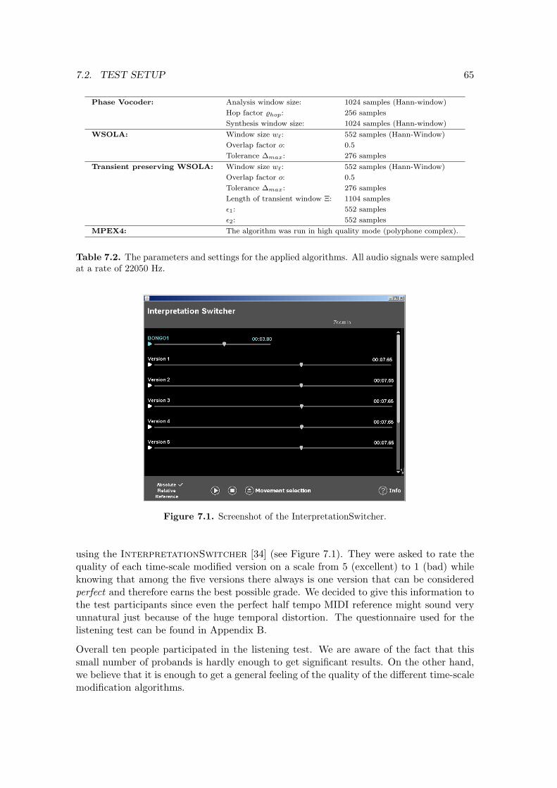
7.2. TEST SETUP 65
Phase Vocoder: Analysis window size: 1024 samples (Hann-window)
Hop factor hop: 256 samples
Synthesis window size: 1024 samples (Hann-window)
WSOLA: Window size wℓ: 552 samples (Hann-Window)
Overlap factor o: 0.5
Tolerance ∆max: 276 samples
Transient preserving WSOLA: Window size wℓ: 552 samples (Hann-Window)
Overlap factor o: 0.5
Tolerance ∆max: 276 samples
Length of transient window Ξ: 1104 samples
ǫ1: 552 samples
ǫ2: 552 samples
MPEX4: The algorithm was run in high quality mode (polyphone complex).
Table 7.2. The parameters and settings for the applied algorithms. All audio signals were sampledat a rate of 22050 Hz.
Figure 7.1. Screenshot of the InterpretationSwitcher.
using the InterpretationSwitcher [34] (see Figure 7.1). They were asked to rate thequality of each time-scale modified version on a scale from 5 (excellent) to 1 (bad) whileknowing that among the five versions there always is one version that can be consideredperfect and therefore earns the best possible grade. We decided to give this information tothe test participants since even the perfect half tempo MIDI reference might sound veryunnatural just because of the huge temporal distortion. The questionnaire used for thelistening test can be found in Appendix B.
Overall ten people participated in the listening test. We are aware of the fact that thissmall number of probands is hardly enough to get significant results. On the other hand,we believe that it is enough to get a general feeling of the quality of the different time-scalemodification algorithms.
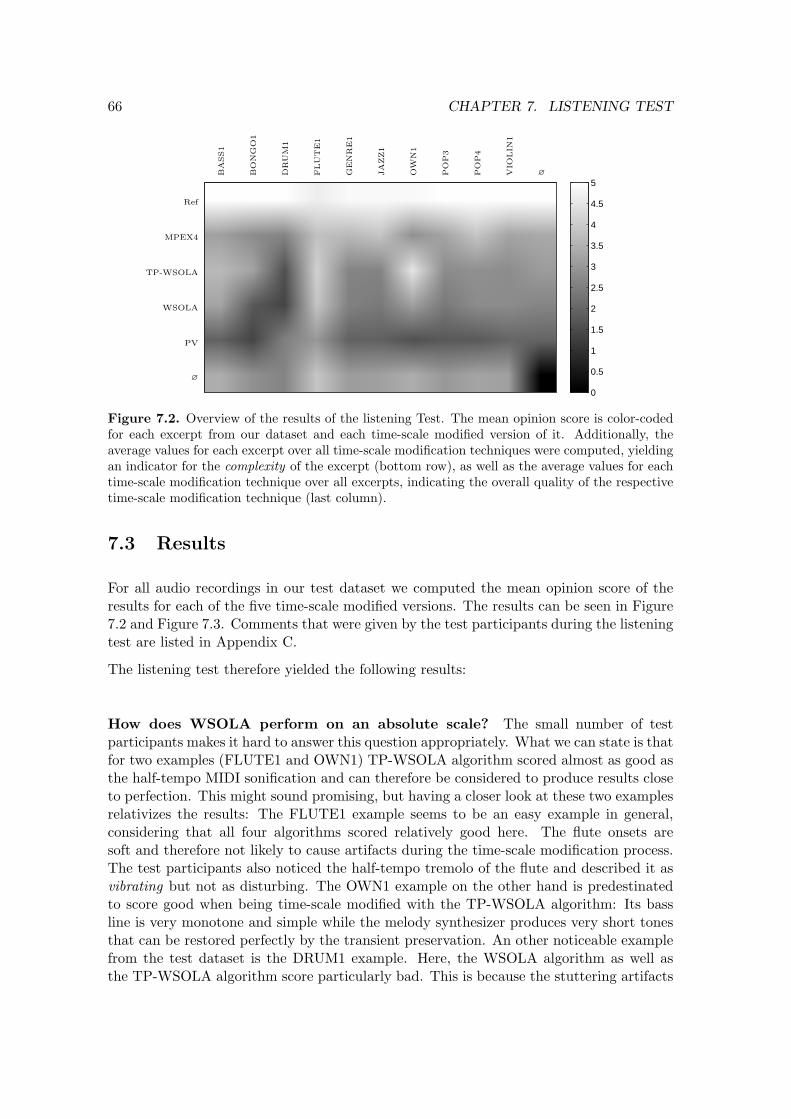
66 CHAPTER 7. LISTENING TEST
0
0.5
1
1.5
2
2.5
3
3.5
4
4.5
5
BASS1
BONGO1
DRUM
1
FLUTE1
GENRE1
JAZZ1
OW
N1
POP3
POP4
VIO
LIN
1
∅
Ref
MPEX4
TP-WSOLA
WSOLA
PV
∅
Figure 7.2. Overview of the results of the listening Test. The mean opinion score is color-codedfor each excerpt from our dataset and each time-scale modified version of it. Additionally, theaverage values for each excerpt over all time-scale modification techniques were computed, yieldingan indicator for the complexity of the excerpt (bottom row), as well as the average values for eachtime-scale modification technique over all excerpts, indicating the overall quality of the respectivetime-scale modification technique (last column).
7.3 Results
For all audio recordings in our test dataset we computed the mean opinion score of theresults for each of the five time-scale modified versions. The results can be seen in Figure7.2 and Figure 7.3. Comments that were given by the test participants during the listeningtest are listed in Appendix C.
The listening test therefore yielded the following results:
How does WSOLA perform on an absolute scale? The small number of testparticipants makes it hard to answer this question appropriately. What we can state is thatfor two examples (FLUTE1 and OWN1) TP-WSOLA algorithm scored almost as good asthe half-tempo MIDI sonification and can therefore be considered to produce results closeto perfection. This might sound promising, but having a closer look at these two examplesrelativizes the results: The FLUTE1 example seems to be an easy example in general,considering that all four algorithms scored relatively good here. The flute onsets aresoft and therefore not likely to cause artifacts during the time-scale modification process.The test participants also noticed the half-tempo tremolo of the flute and described it asvibrating but not as disturbing. The OWN1 example on the other hand is predestinatedto score good when being time-scale modified with the TP-WSOLA algorithm: Its bassline is very monotone and simple while the melody synthesizer produces very short tonesthat can be restored perfectly by the transient preservation. An other noticeable examplefrom the test dataset is the DRUM1 example. Here, the WSOLA algorithm as well asthe TP-WSOLA algorithm score particularly bad. This is because the stuttering artifacts

7.3. RESULTS 67
1
2
3
4
5
Ref
MPEX4
TP−WSOLA
WSOLA PV
BASS1
1
2
3
4
5
Ref
MPEX4
TP−WSOLA
WSOLA PV
BONGO1
1
2
3
4
5
Ref
MPEX4
TP−WSOLA
WSOLA PV
DRUM1
1
2
3
4
5
Ref
MPEX4
TP−WSOLA
WSOLA PV
FLUTE1
1
2
3
4
5
Ref
MPEX4
TP−WSOLA
WSOLA PV
GENRE1
1
2
3
4
5
Ref
MPEX4
TP−WSOLA
WSOLA PV
JAZZ1
1
2
3
4
5
Ref
MPEX4
TP−WSOLA
WSOLA PV
OWN1
1
2
3
4
5
Ref
MPEX4
TP−WSOLA
WSOLA PV
POP3
1
2
3
4
5
Ref
MPEX4
TP−WSOLA
WSOLA PV
POP4
1
2
3
4
5
Ref
MPEX4
TP−WSOLA
WSOLA PV
VIOLIN1
Figure 7.3. Results of the listening test for the half-tempo MIDI reference (Ref), the MPEX4algorithm, TP-WSOLA, WSOLA and the Phase Vocoder (PV). The standard deviation is indicatedby red bars.

68 CHAPTER 7. LISTENING TEST
0 0.5 1 1.5 2 2.5 3
0 0.5 1 1.5 2 2.5 3
0 0.5 1 1.5 2 2.5 3
0 0.5 1 1.5 2 2.5 3
(a)
(b)
(c)
(d)
Figure 7.4. (a) The waveform of the first 3 seconds from the half-tempo MIDI reference ofDRUM1. (b) The spectrogram related to (a). Note the rather long decay phases of the notesresulting from room reverb. (c) The waveform of the first 3 seconds from DRUM1 stretched witha time-scale factor of 2 using TP-WSOLA. (d) The spectrogram related to (c). Note that a lot ofstuttering artifacts are visible in the decay phases of the notes even though the actual onsets arepreserved by the algorithm.
cause an electric and metallic sound of the drums. The stuttering artifacts also occurwhen using TP-WSOLA because of the room reverb in this example (See Figure 7.4).Summarizing we can say that the quality of time-scale modified audio signals producedwith WSOLA strongly depend on the input audio signal.
How does WSOLA perform in comparison to other time-scale modificationalgorithms? For most of the examples in our test dataset WSOLA and TP-WSOLAalgorithm perform slightly worse than the commercial MPEX4 algorithm and slightlybetter than the Phase Vocoder. But unlike MPEX4, which robustly yields rather goodresults for almost any example, the quality of results for WSOLA is much more signaldependent.In this context, it is also important to point out that the commercial MPEX4 and ourMATLAB implementation of WSOLA differ significantly concerning the running time:while our WSOLA implementation takes about one to two seconds to compute the time-scale modification of an audio signal of roughly five seconds with a constant time-stretchfactor of two, the MPEX4 algorithm in its highest quality mode (in which we run thealgorithm for our listening test) needs about 20 seconds.
How great is the effect of transient preservation in WSOLA? We can observethat on average TP-WSOLA scores always better or equal to the standard WSOLA. In

7.3. RESULTS 69
0 0.5 1 1.5
0 0.5 1 1.5 2
0 0.5 1 1.5
0 0.5 1 1.5 2
(a)
(b)
(c)
(d)
Figure 7.5. (a) The waveform of the first 2 seconds from BONGO1 stretched with a time-scalefactor of 2 using WSOLA. (b) The spectrogram related to (a). Note that the stuttering artifactsare visible very well. (c) The waveform of the first 2 seconds from BONGO1 stretched with atime-scale factor of 2 using TP-WSOLA. (d) The spectrogram related to (c). One can observethat the transient preservation reduces stuttering artifacts at transients significantly. This can beseen in the waveform (steep attack phase and steady decay phase with transient preservation) aswell as in the spectrogram (sharper transient regions in the spectrogram).
some cases it even causes huge quality improvements. Examples for this improvements areBONGO1 and OWN1, where TP-WSOLA scores significantly better than the standardWSOLA. Again this is mainly due to the structure of those audio signals. The short bongohits in BONGO1 as well as the short noise-like bursts of the melody synthesizer in OWN1can be restored perfectly by the transient preservation during the time-scale modification.On the other hand, these bursts also cause major stuttering artifacts when time-scalemodifying with the standard WSOLA technique (see Figure 7.5). For other instrumentslike for example the bass in BASS1 the stuttering artifacts are not that well perceivableand the score difference is therefore not that high. For examples like VIOLIN1, where verylittle note onsets occur and the onsets are also rather soft there is virtually no differencebetween the standard WSOLA and its transient preserving version.

70 CHAPTER 7. LISTENING TEST

Chapter 8
The Connector’s Pipeline
The purpose of the Connector is to produce a transition from a given audio recording toanother audio recording in a database that fulfills given constraints. This transition shouldbe as pleasant as possible to the ear of the listener. Of course, pleasant is a very vagueterm in this context. There are extremely many aspects of the audio signals that couldcount towards the quality of a produced transition like harmony, beat progression, genre,timbre, volume or even just the quality of the audio recordings that are used. Furthermore,it is hard to argue about what sounds pleasant to everybody since the same transitionmight sound differently appealing to different people. The Connector therefore focuseson those aspects that are, at least intuitively, generally important when it comes to theeuphony of transitions which are the harmonic progression and the beat. In this chapterwe describe the Connector in its current state.
Given to the Connector are an audio recording for which a transition region is specifiedalong with a set of user defined constraints. The transition region marks the part in theaudio recording where the transition to another audio recording should take place. Likeshown in Figure 1.3, the Connector works in three stages. In the matching stage, theaudio in the transition region is converted into a suitable representation that allows tofind other audio recordings with regions that share a similar harmonic progression in adatabase. Picking the best match that fulfills all constraints specified by the user givesus the audio recording that we will bridge to. The region in this audio recording that issimilar in its harmonic progression to the transition region is referred to as the matchedregion. At this point, the warping stage of the Connector starts. The goal of this stageis to rhythmically synchronize the transition region with the matched region. This is doneby applying TSM algorithms to both regions such that afterwards the beat positions ofboth regions are temporally aligned. The idea of synchronizing the beats while bridgingfrom one audio recording to another originates from the field of DJing. Since the beat isa very important element in danceable music, it allows the DJ to create extremely longaudio recordings that are danceable from the beginning to the end without breaks (seefor example [3]). This continuity is exactly what we want to maintain during a transition.In the last stage of the Connector the two audio recordings are blended by overlayingthe transition region and the matched region and applying a simple crossfade. Since bothregions are now similar in their harmonic progression and rhythmically synchronized, the
71

72 CHAPTER 8. THE CONNECTOR’S PIPELINE
transition should sound euphonious.
This chapter is structured as follows. In Section 8.1 we introduce other work in the fieldof music generation. In Section 8.2 and Section 8.3 we explain the matching process indetail while we discuss the structure of our database in Section 8.4. Finally we have a fewremarks on the warping and the blending stage of the Connector in Sections 8.5 and8.6.
8.1 Related Work
The idea of connecting existing music by creating euphonious transitions to generate newmusic is not a recent one. At the end of the 18th century, Musikalische Wurfelspiele werea popular pastime. In this game a piano player had to compose music by concatenatingmeasures from known pieces that were randomly chosen by the roll of a dice [22, 16].Nowadays this idea has shifted towards the digital world. In times were large amounts ofmusical scores are available in the form of MIDI data, an automated music generation sys-tem based on these files is proposed in [6]. This approach works in the so called symbolicdomain which means that it does not deal with existing audio signals but with some ab-stract representation of music. Music generation in the symbolic domain can be consideredeasier to be handled than music generation in the audio domain since the abstract repre-sentation allows for much more flexibility. Unfortunately to be able to listen to music inthe symbolic domain it either needs to be played by human performers or synthesized by amachine. But since human performances are expensive and synthesized music is typicallyinferior in quality to real world audio recordings, music generation in the symbolic domainis often not an option. But there also exist approaches working in the audio domain. Amodern field in which techniques to concatenate audio recordings in an appealing way arevery important is the field of DJing [3]. While for a DJ the harmonic similarity of twoconnected audio recordings usually plays a minor role, a good rhythmical transition is es-sential. A tool to automate the process of finding good rhythmical transitions between twoaudio recordings automatically is proposed in [24]. The work of [30] comes closest to ourapproach. It describes a framework that allows to concatenate a set of audio recordingsto a single long audio recording. The audio recordings are ordered such that euphonioustransitions between the clips are possible. The positions of the transitions are chosen tomaximize the local harmonic and rhythmic similarity of the two audio recordings. Thework of [45] aims to synthesize a soundtrack for a given visual data stream from a singleaudio recording, the so called example. By linking events in the visual data stream withspecific parts in the example the complete soundtrack can be rendered.
The approach of concatenating audio recordings can even be used to synthesize new soundsrather than complete audio recordings. To this end audio recordings are analyzed andsegmented in short units. This is done for large collections of audio data. The units canthen be used to synthesize target sounds by rearranging them. This technique is calledConcatenative Sound Synthesis and is described in [38, 39, 40, 41].

8.2. MATCHING 73
8.2 Matching
In the first stage of the Connector an audio recording should be found in a database thatis at some point similar in its harmonic progression to the transition region. We thereforefirst need an appropriate representation of audio signals that allows for comparing themin terms of harmonic content. The chroma features introduced in Chapter 2 have shownto capture the desired property very well. They abstract away from instrumentation andtimbre information and are designed to solely focus on the tonal content of the audiosignal. Unfortunately they do not abstract away from timing information since they arecomputed at a fixed rate. Although this is in general a desirable property, in the context oftheConnector this would make the matching process rather complicated. In the simplestcase we can state similarity in harmonic progression if we have two feature sequences ofthe same length and the features can be considered similar pairwise. But assume we wantto compare the feature representation of two interpretations of the same musical piece andassume further that one of the two interpretations was performed at half the tempo of theother. We know that the harmonic progression of both interpretations is exactly the same,but we can not compare the two feature sequences since they are not of the same length.There exist techniques that allow for finding similarities in feature sequences where thecompared sequences do not need to be of the same length (Dynamic Time Warping [33])but these techniques are computationally rather expensive in comparison to the naiveapproach. Furthermore it has shown that not only the harmonic similarity is importantto get euphonious results when blending from one audio recording to another, but alsothe alignment of the beats in both audio recordings. Therefore it is important that theharmonic similarity still exists after the temporal alignment of the beats in the transitionregion and the matched region. The solution to this issue are the beat-synchronous chromafeatures that were also introduced in Chapter 2. Since these features use the musical beat-level as their time axis we can avoid matching techniques like Dynamic Time Warpingand use the naive approach of comparing two feature sequences of the same length bypairwise comparison of the features. Furthermore this also solves the problem of keepingthe harmonic content of two audio recordings similar after the alignment of their beatpositions since by design of the beat-synchronous chroma features two feature sequencesare similar exactly in case the two underlaying audio recordings share a similar harmonicprogression on the beat level.
Note that to compute the beat-synchronous features it is essential to know all beat posi-tions of the underlaying audio recording. These could for example be extracted by usinga beat tracker. Unfortunately the problem of beat tracking is not solved completely so farsince the task is rather hard for some kinds of music like for example violin music [21].Although there already exist a lot of approaches, like for example in [8, 28, 2, 13], thereexists no beat tracker to our knowledge that could reliably predict the beat positions foraudio recordings of all kinds of music. But since we want to work on a large variety ofdifferent musical styles we just avoid this problem for the moment and assume all beatpositions for all audio recordings to be given. We therefore use a fully beat annotateddatabase in which all beat positions of all audio recordings are annotated manually.
The matching technique that we use in the Connector was introduced in [35]. Givena query audio signal, which is the transition region in our case, for which we computed

74 CHAPTER 8. THE CONNECTOR’S PIPELINE
C C#D D#E F
F#G
G#A A#B
C C#D D#E F
F#G
G#A A#B
Q
D
Figure 8.1. Visualization of the task of audio matching. Given a sequence of beat-synchronouschroma vectors Q computed from our query audio signal, we want to find a subsequence of chromavectors in the database D such that the chroma vectors can be considered similar pairwise. For thisexample the database was chose to be extremely small for visualization purposes. The subsequenceof chroma vectors that is most similar to the query sequence is marked by a green box.
beat-synchronous chrome features, our goal is to find a segment in an audio recording froma database that has a similar harmonic progression to our query audio signal on the beatlevel. It is therefore important that the database holds beat-synchronous chroma featuresof all contained audio recordings as well. To this end, we can simply see the databaseas a concatenation of the beat-synchronous chroma features of all audio recordings thatare included in the database. Additionally we keep track of the boundaries in a separatedata-structure. It is therefore possible to map a certain chroma vector in the databaseto a decisive position in a decisive audio recording. We now need to find a sequence ofchroma vectors in the database that can be considered similar to the sequence computedfrom our query audio signal. Figure 8.1 illustrates this task.
The first step towards this goal is to define a distance measure for chroma vectors. Recallthat all chroma vectors we work with are normalized. Therefore the inner product of twochroma vectors ~x and ~y, which is denoted by 〈~x, ~y〉 coincides with the cosine of the anglebetween ~x and ~y and therefore quantizes the distance of ~x and ~y. For this reason we simplydefine our distance measure δ as
δ(~x, ~y) = 1− 〈~x, ~y〉 (8.1)
Note that 〈~x, ~y〉 ∈ [0, 1] and therefore also δ(~x, ~y) ∈ [0, 1]. To extend this distance measureto sequences of features ~X = (~x1, ~x2, ..., ~xL) and ~Y = (~y1, ~y2, ..., ~yL) of the same length Lwe define
δL( ~X, ~Y ) =1
L
L∑
ℓ=1
δ(~xℓ, ~yℓ) (8.2)
Having the query sequence of chroma vectors ~Q = (~q1, ~q2, ...~qM ) and the sequence ofdatabase chroma vectors ~D = (~d1, ~d2, ...~dN ) where M < N we can now define the distance

8.2. MATCHING 75
function ∆ : [1 : n]→ [0, 1] by
∆(i) = δM ((~q1, ~q2, ...~qM ), (~di, ~di+1, ...~di+M−1)) (8.3)
for i ∈ [1 : N −M + 1] and
∆(i) = 1 (8.4)
for i ∈ [N−M+2 : N ]. The value ∆(i) describes the distance between the query sequenceof chroma vectors and the subsequence of database chroma vectors starting with the ith
vector.
Notice that the function ∆ can be computed very easily. This is the case since we cancompute all interesting values of the distance measure δ by a single matrix multiplication.Recall that we can write
Q = (~q1, ~q2, · · · , ~qM ) =
q12,1 q12,M...
...
q2,1 q2,2q1,1 q1,2 · · · q1,M
D = (~d1, ~d2, · · · , ~dN ) =
d12,1 d12,N...
...
d2,1 d2,2d1,1 d1,2 · · · d1,N
(8.5)
where Q ∈ R12×M and D ∈ R12×N . Now we can compute the matrix
C =1
M· (1M×N −QT ·D) (8.6)
where 1M×N ∈ RM×N is the matrix for which all entries are 1. The matrix C has theform
C = 1M ·
1− 〈~qM , ~d1〉 1− 〈~qM , ~dN 〉...
...
1− 〈~q2, ~d1〉 1− 〈~q2, ~d2〉
1− 〈~q1, ~d1〉 1− 〈~q1, ~d2〉 · · · 1− 〈~q1, ~dN 〉
= 1M
δ(~qM , ~d1) δ(~qM , ~dN )...
...
δ(~q2, ~d1) δ(~q2, ~d2)
δ(~q1, ~d1) δ(~q1, ~d2) · · · δ(~q1, ~dN )
(8.7)

76 CHAPTER 8. THE CONNECTOR’S PIPELINE
query
database
~q1
~q2
.
.
.
~qM~d1 ~d2 · · · ~dM ~dM+1 · · · ~dN
∆(1) ∆(2) ∆(3) · · · ∆(N −M + 1)
· · ·
Figure 8.2. An abstract representation of the matrix C. The diagonal lines represent the entriesthat are summed up to get the entries of ∆.
Therefore we have that
M∑k=1
Ck,i+k−1 = 1M ·
M∑k=1
δ(~qk, ~di+k−1) (8.7)
= δM ((~q1, ~q1, ...~qM ), (~di, ~di+1, ...~di+M−1)) (8.2)= ∆(i) (8.3)
(8.8)
This computation is visualized in Figure 8.2. To find the subsequence of chroma vectors inthe database that is maximal similar to the query sequence of chroma vectors we can nowsimply pick the index i in ∆ such that ∆(i) is minimal. The index i then marks the firstvector of the best matching subsequence in the database. Figure 8.3 shows an example ofthe matching process.
8.3 Query Pool
To increase the possibility of finding a match in the database that is very similar in itsharmonic progression to the transition region it is helpful to give the matching processsome degrees of freedom. These degrees of freedom are musically motivated and cantherefore be expressed as modifications of the beat-synchronous chroma features of thetransition region. We separate the degrees of freedom into three subclasses.
The position tolerance allows to temporally shift the transition region by up to a certainamount of beats. This relaxes the constraint on where exactly the transition to anotheraudio recording should take place (see Figure 8.4).
The pitch tolerance accounts for the fact that it is possible to pitch shift every audiorecording in the database by a small amount of semitones without significant audio degra-
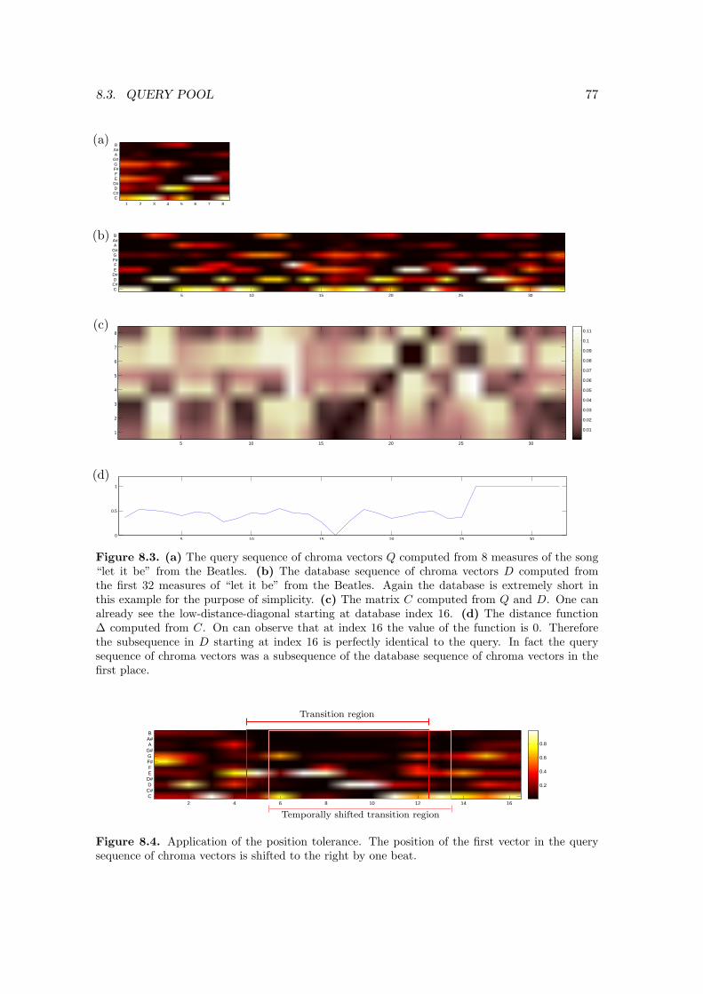
8.3. QUERY POOL 77
5 10 15 20 25 300
0.5
1
5 10 15 20 25 30
1
2
3
4
5
6
7
8
0.01
0.02
0.03
0.04
0.05
0.06
0.07
0.08
0.09
0.1
0.11
5 10 15 20 25 30C C#D D#E F
F#G
G#A A#B
1 2 3 4 5 6 7 8C C#D D#E F
F#G
G#A A#B
(a)
(b)
(c)
(d)
Figure 8.3. (a) The query sequence of chroma vectors Q computed from 8 measures of the song“let it be” from the Beatles. (b) The database sequence of chroma vectors D computed fromthe first 32 measures of “let it be” from the Beatles. Again the database is extremely short inthis example for the purpose of simplicity. (c) The matrix C computed from Q and D. One canalready see the low-distance-diagonal starting at database index 16. (d) The distance function∆ computed from C. On can observe that at index 16 the value of the function is 0. Thereforethe subsequence in D starting at index 16 is perfectly identical to the query. In fact the querysequence of chroma vectors was a subsequence of the database sequence of chroma vectors in thefirst place.
2 4 6 8 10 12 14 16C C#D D#E F
F#G
G#A A#B
0.2
0.4
0.6
0.8
Transition region
Temporally shifted transition region
Figure 8.4. Application of the position tolerance. The position of the first vector in the querysequence of chroma vectors is shifted to the right by one beat.

78 CHAPTER 8. THE CONNECTOR’S PIPELINE
1 2 3 4 5 6 7 8C C#D D#E F
F#G
G#A A#B
1 2 3 4 5 6 7 8C C#D D#E F
F#G
G#A A#B
Transition region Pitch shifted transition region
Figure 8.5. Application of the pitch tolerance. By vertically cyclic shifting the chroma vectorsby one, a match for this modified sequence of chroma vectors that is found in the database isharmonically similar to the transition region if pitched down by one semitone.
1 2 3 4 5 6 7 8C C#D D#E F
F#G
G#A A#B
1 2 3 4C C#D D#E F
F#G
G#A A#B
2 4 6 8 10 12 14 16C C#D D#E F
F#G
G#A A#B
Transition region
Half-time transition region
Double-time transition region
Figure 8.6. Application of the type of meter tolerance. By either expanding the sequence ofchroma vectors by doubling every chroma vector or compressing it by averaging two neighboredchroma vectors it is possible to find harmonically similar matches in the database that have adifferent beat resolution than the original transition region.
dation. To emulate such a pitch shift, chroma vectors of the transition region are simplycyclic shifted vertically by the desired amount of semitones (see Figure 8.5).
The type of meter tolerance allows for changing the beat resolution during the transitionphase to half-time or double-time. This is helpful since the the beat of an audio recordingmay be perceived on different resolutions and is therefore ambiguous. Without the typeof meter tolerance, two recordings that share the exact same harmonic progression cannot be matched in case the beat of the two audio recordings is annotated on differentresolutions. To emulate the different beat resolutions, the sequence of chroma vectors ofthe transition region is either expanded by doubling every single chroma vector (double-time) or compressed by averaging two neighbored chroma vectors (half-time) (see Figure8.6).
By applying these modifications and combinations of them to the original query sequenceof chroma vectors we extend the single query sequence to a query pool. Instead of matchingonly one sequence of chroma vectors with the database, we sequentially match all sequencesin the query pool with the database and pick the one that yielded the match with the

8.4. DATABASE 79
lowest distance value in the end.
8.4 Database
The matching technique described in Section 8.2 needs the database to have the formof a single long sequence of chroma vectors. Therefore the chromagrams of all audiorecordings in the database are concatenated and we keep track of the boundaries in aseparate data structure. Additionally, we store further informations about every includedaudio recording like for example the name of the sound file and the temporal positions ofall beats on which the computation of the beat synchronous chroma features was based.The latter information is very important since the beat synchronous chroma features donot hold any temporal information anymore by themselves.
A problem that might occur when representing the database as a concatenation of thechromagrams of all includes audio recordings is that the subsequence of chroma vectors inthe database that is most similar to the query sequence of chroma vectors might containchroma vectors from two different audio recordings. The solution to this problem is to padthe sequences of chroma vectors of all audio recordings with a sequence of zero-vectorswhich is at least of the same length as the query sequence of chroma vectors. The effectof this zero-pad is visualized in Figure 8.7.
8.5 Warping
Having developed a good TSM algorithm in Chapter 6, we now can use this algorithm torhythmically synchronize the transition region and the matched region. This is done by atemporal alignment of the beat positions of the two audio clips. The goal is therefore tocompute two time-stretch functions τtr for the transition region and τmr for the matchedregion such that when overlaying the results of the time-scale modifications of both audioclips their beat positions are aligned. Figure 8.8 shows an example. Note that both thetransition region as well as the matched region have the same length on the beat level bydesign of the matching process. We define this number of beats to be N . Let the sequenceof beat positions in the transitions region given in seconds be
T = t1, t2, ..., tN (8.9)
and the sequence of beat positions in the matched region
M = m1,m2, ...,mN (8.10)
while it holds that q1 = 0 and m1 = 0. We now have to define a sequence of beat positions
S = s1, s2, ..., sN (8.11)

80 CHAPTER 8. THE CONNECTOR’S PIPELINE
5 10 15 20 25 30 350
0.5
1
5 10 15 20 25 30 35C C#D D#E F
F#G
G#A A#B
5 10 15 20 25 300
0.5
1
5 10 15 20 25 30C C#D D#E F
F#G
G#A A#B
1 2 3 4 5 6 7 8C C#D D#E F
F#G
G#A A#B
audio recording A audio recording B
audio recording A audio recording Bzeropad
(a)
(b)
(c)
(d)
(e)
Figure 8.7. (a) The sequence of query chroma vectors. (b) A sequence of database chromavectors consisting of two audio recordings. The chromagrams are not separated by a zero pad.(c). The distance function ∆ computed from the query chromagram from (a) and the databasechromagram from (b). The subsequence of chroma vectors in the database that is most similar tothe query sequence of chroma vectors (marked by green box in (b)) contains chroma vectors fromtwo different audio recordings. (d) The database chromagram from (b) with a zeropad betweenthe two songs. (e) The distance function ∆ computed from the query chromagram from (a) andthe database chromagram from (d). The zeropad prevents the distance function from having smallvalues at audio recording boundaries.
t1 t2 t3 t4 t5 t6 t7 t8 t9
m1 m2 m3 m4 m5 m6 m7 m8 m9
T
τtr
S
τmr
M
Figure 8.8. An example of the computations of τtr and τmr.

8.6. BLENDING 81
that we can use to define the time-stretch functions τQ and τM by sets of anchor points
τQ = ((t1, s1), (t2, s2), ..., (tN , sN ))τM = ((m1, s1), (m2, s2), ..., (mN , sN ))
(8.12)
The sequence S should be chosen such that the tempo of the transition region smoothlyadapts to the tempo of the matched region. We therefore define
s1 = 0
si = si−1 +N−(i−1)
N · (ti − ti−1) +i−1N · (mi −mi−1) for i ∈ [2 : N ]
(8.13)
The transition region as well as the matched region are then time-scale modified using thetime-stretch functions τtr and τtm respectively.
8.6 Blending
To finish the transition we now overlay the transient region with the matched region andapply a simple blending. Blending is the process of making the transition between twoaudio recordings less abrupt. The simplest kind of blending is the so called crossfade.By decreasing the volume of the transition region until it is finally not perceivable anymore while at the same time increase the volume of the matched region from silence tothe normal volume, a smooth transitions between the two clips is created. Although therealso exist more advanced blending techniques the simple crossfade technique suffices ourneeds.
The whole pipeline of the Connector is summarized in Figure 8.6.

82 CHAPTER 8. THE CONNECTOR’S PIPELINE
C C#D D#E F
F#G
G#A
A#B
C C#D D#E F
F#G
G#A
A#B
C C#D D#E F
F#G
G#A
A#B
C C#D D#E F
F#G
G#A
A#B
C C#D D#E F
F#G
G#A
A#B
C C#D D#E F
F#G
G#A
A#B
C C#D D#E F
F#G
G#A
A#B
MATCHING
WARPING
BLENDING
Transition region
Currently playing audio
Beat annotation Pitch feature
Beat-synchronous chroma feature
Database
Query pool
Best matching audio
Transition region
Matched region
Synthesized result
+
find best match
possibly pitch shift
TSM crossfade
Figure 8.9. Overview of the Connector.

Chapter 9
Future Work
In this thesis, we discussed various time-scale modification algorithms and their applicationto music audio signals. In particular, we analyzed WSOLA as an example of a time-domainalgorithm and the Phase Vocoder as an example of a frequency domain algorithm. Fur-thermore we introduced modifications to the WSOLA algorithm which reduce artifacts inthe algorithm’s output by preserving transients during the time-scale modification process.Although this already increases the quality of WSOLA significantly, we feel that there isstill a lot of room for improvements. As already briefly discussed in Chapter 4, WSOLAoften has problems when time-scale modifying signals of high complexity like for examplerecordings of orchestral music. This kind of audio signals are highly polyphonic due to thepresence of many instruments that play different notes. Therefore numerous fundamentalfrequencies exist in such signals. However, WSOLA is only capable of preserving a singlefundamental frequency. As a consequence, the remaining fundamental frequencies are notpreserved properly and phase jump artifacts are introduced which manifest themselves ina metallic, noise-like sound. An idea to overcome this phenomenon is to split the inputsignal into several subbands prior to the time-scale modification. The subbands are thentime-scale modified seperatly and added up afterwards. Every single subband is of courseless complex than the original input signal. Therefore the time-scale modification of a sin-gle subband should yield significantly less artifacts than the time-scale modification of theoriginal signal and therefore also the sum of all time-scale modified subband signals shouldsuffer less from artifacts. This idea is inspired by the Phase Vocoder which ensures phasecontinuity for a very fine-grained frequency decomposition of the input signal. But thisfine decomposition is also responsible for the loss of vertical phase coherence in the outputsignal which causes the artifacts that are typical for the Phase Vocoder. By choosing thenumber of subbands to be rather low, namely to be in the magnitude of the number offundamental frequencies in the input signal, the loss of vertical phase coherence should beprevented.
On the application side we see a lot of potential in theConnector. For example, althoughour matching technique already yields matches that are of a similar harmonic content asthe transition region, it could be further improved by techniques from the field of chordrecognition. During the matching process, we select matches based on the assumption thatthe similarity of two sequences of chroma vectors yields a strong indication for harmonic
83

84 CHAPTER 9. FUTURE WORK
similarity. But in fact the numerical similarity of the sequences of chroma vectors is noguarantee for a perceptual similarity. For example the major and minor chords for acertain root note only differ in a single chroma value and may therefore be matched. Butchanging the harmony from major to minor during a transition often sounds unpleasant.Furthermore it is likely that the euphony of a transition is not only dependent on theharmonic structure of the transition region, but also on the chord progression on a largerscale.
A further improvement of the Connector can be done in its blending stage. The simplecrossfade that we apply during the transition can be replaced by some more advancedblending technique. Experiments have shown that it is for example sometimes convenientto blend different instruments in an audio signal in a different way or at different pointsin time. To this end, source separation techniques can be applied to the audio signals toget the functionality of an instrument equalizer.
In conclusion, we have seen that time-scale modification is a central topic in audio signalprocessing with various applications such as automated soundtrack generation. In partic-ular, in the context of the Connector, it has shown that time-scale modification needsto be combined with further music analysis and retrieval tasks, including beat tracking,chord recognition, source separation and audio matching. For the future, we plan to fur-ther automate the various components of the Connector and to develop tools that allowusers to easily search for, modify, merge, and generate suitable soundtracks.

Appendix A
Source Code
In this chapter, the header of our MATLAB implementation of TP-WSOLA that wasdescribed in Chapter 6 and that was created during the writing of this thesis is given.
Sample usage:parameter.automatedTransientPreservation = 1;
y = tp_wsola(x, 2, parameter);
%%%%%%%%%%%%%%%%%%%%%%%%%%%%%%%%%%%%%%%%%%%%%%%%%%%%%%%%%%%%%%%%%%%%%%%%%%%
% Name: tp_wsola
% Version: 1.0
% Date: 5.10.2011
% Programmer: J. Driedger ([email protected])
%
% Description:
% tp_wsola is a transient preserving time-scale modification algorithm
% based on the WSOLA algorithm. It is capable of preserving transients
% automatically as well as preserving transients at additionally given
% positions.
%
% Input:
% y = wsola(x,t):
% x: mono / stereo signal (column vector)
% t: either a (n x 2) matrix containing anchor points specified in
% samples or seconds or a constant time-stretch factor.
%
% Optional input arguments:
% y = wsola_core(x,t,parameter):
% parameter.windowSize: specifies the size of the Hann-window that is
% used for input and output.
% parameter.tolerance : specifies the tolerance Delta_max for the input
% window positions.
% parameter.APStyle : Is either ’samples’ or ’seconds’ and specifies
% how the given anchor points are interpreted.
% parameter.samplerate: specifies the samplingrate of the audio.
% parameter.automatedTransientPreservation:
% Should be set to 1 in case transients should be
85

86 APPENDIX A. SOURCE CODE
% detected and preserved automatically.
% parameter.preservedPositions:
% Additional positions of transients that should be
% preserved.
% parameter.transientWindowSize:
% The size of the transient window Xi.
%
% Output:
% y: time-scale midified output signal (mono / stereo)
%%%%%%%%%%%%%%%%%%%%%%%%%%%%%%%%%%%%%%%%%%%%%%%%%%%%%%%%%%%%%%%%%%%%%%%%%%%

Appendix B
Listening Test Questionnaire
The questionnaire that was used for the listening test to rate the quality of differenttime-scale modification algorithms (Section 7).
87

88 APPENDIX B. LISTENING TEST QUESTIONNAIRE
Instructions
The aim of this evaluation is to rate the quality of different audio time-scale modificationtechniques. Time-scale modification algorithms allow us to change the speed on whichan audio recording is played without altering the pitch of the audio. They are intendedto produce versions of an audio recording that sound as if the musical piece was initiallyperformed on a different tempo. In the following we will present you with a couple of dif-ferent audio recordings along with several time-scale modified versions of them which wereproduced using different time-scale modification algorithms. The original audio record-ings were created synthetically and may therefore sound a little unnatural. All modifiedversions are double the length of the original audio recordings. We ask you to rate thequality of the manipulated versions on a scale from 5 (excellent) to 1 (bad). To give youa reference for your evaluation there will always be a version that is simply the originalrecording synthesized on half the tempo. This version can therefore be seen as the resultof a perfect time-scale modification algorithm.You will be able to listen to the original audio recording and the modified versions asoften as you like but it is important that you listen to each audio recording and eachmodification at least once from the beginning to the end. Feel also free to comment oneverything that occurs to you during the listening test.
EXAMPLE
excel-lent
good fair poor bad Comment
5 4 3 2 1
Version 1 ©⊗
© © © something was wrong withthe pitch
Version 2 ©⊗
© © ©
Version 3⊗
© © © © sounded perfect!
Version 4 © © © ©⊗
had nothing to do with theoriginal...
Version 5 © © ©⊗
© beginning was good, butscrewd up at the end
Additional Comments: The quality was in general hard to tell since this example is pretty stupid.

Appendix C
Listening Test Comments
In the following the comments that were given by the listening test participants duringthe listening test are listed.
Name Algorithm Comments
BASS1 MPEX4 slightly wrong notes — slightly stuttering at the beginning but 2ndhalf was good — strange chorus like effect — quick tone changes donot sound well — quite an echo these artifacts
trans. prev. WSOLA artifacts at the beginning/end — slightly wrong notes — slightlystuttering at the beginning but 2nd half was good — at thebeginning of each tone quite some artifacts
WSOLA artifacts in higher pitches — unclean note transitions at the end —slightly stuttering — a little bit vibrating — artifacts — at thebeginning of each tone there were artifacts
Phase Vocoder lower volume? — no clean tones — stuttering — dynamics killed?— higher frequencies cut off — because the sound is vibrating —attacks do not sound well — somehow crumbly
BONGO1 MPEX4 delay effect, small artifacts on higher drums — echo/doubled notes— slight stuttering — strange onset. sounds like after using acompressor — attacks are duplicated — the sound is interesting butnot right
trans. prev. WSOLA higher pitches bad, lower good — slight echo — the beats soundstretched — stretches too long (bongos sound artificial) — thesound lost some corpus — it sounds empty
WSOLA electric sound — stuttering — metallic sound — seems to have noise— attacks are duplicated — doesnt sound like a bongo anymore
Phase Vocoder echo — doubled notes — one additional hit every time like shortdelay — pingpong echo — echo of sound happens — attacks areduplicated — too much echo
DRUM1 MPEX4 still lots of artifacts but sounds more homogeneous than others —stuttering — metallic + wobble — wobbly artifacts — electrodrums, but bad bass drum
trans. prev. WSOLA sounds like a synthesizer at higher drums — vibrating notes —stuttering disturbing sound — sounds like beat-mashed — thedrum noises sound as if they are duplicated — the drum became adistorted mess
WSOLA but sounds funny — metallic — stuttering, disturbing sound —metallic — sound quality too low, too much noise — the drumnoises sound as if they are duplicated — electro!!!
Phase Vocoder sounds like a wet room — sligtly metallic — echoing — echo/delay— a little bit echo but okay — the drum noises sound as if they areduplicated — echo
89

90 APPENDIX C. LISTENING TEST COMMENTS
FLUTE1 MPEX4 onsets sounds a little like a glockenspiel — difference to originalhardly noticableonly at the end — vibrating at the ending note —almost perfect but a bit too long
trans. prev. WSOLA little artifact at the end — difference to original hardly noticable —vibrating at the ending note
WSOLA little artifact at the end + glockenspiel onsets — difference tooriginal hardly noticable only in the beginning — vibrating at theending note —could be the original but the long tone at the endsounds strange
Phase Vocoder artifacts at onsets — doubled onset at each note — chorus —vibrating at the ending note — something is strange
GENRE1 MPEX4 drums bad, rest good — metallic drums — stuttering but betterthan others — wobbling — quite good but the instruments do notseem synchronized
trans. prev. WSOLA good drums at the end replaced by electric guitar — stuttering —duplicated attacks — almost perfect but the guitar at the end isstrange
WSOLA lot of artifacts in snare — metallic drums — stuttering — metallic— duplicated attacks — echo and distortion
Phase Vocoder sounds like wet room — metallic and dull — low volume echo —not much survives here — bass guitar almost gone at the end —unbearable, too many artifacts — completely broken
JAZZ1 MPEX4 still some artifacts — sounds “blurry” — ringing sound pitch? —although it seems strange — some reverb
trans. prev. WSOLA Notes somehow wrong, anoying peeptone — distorted — pitchunstable — weird noise after some of the played notes — noise inthe pitch — ”plastic” sound — too distorted
WSOLA lots of artifacts from onsets — notes somehow wrong —distorted —weird noise after some of the played notes — too much noise in thepitch — duplicated attacks + “plastic” — almost broken, cannotstand the chords
Phase Vocoder wet room honkey tonk effect — echo, metallic — like a distant fogpiano but almost “good” — postnuclear piano — nearly cannot tellthe instrument — sounds like “far away” — sounds like plastic
OWN1 MPEX4 wet room — tretching notes misses the fundamental frequencysomehow — stuttering but slightly better — less echo(?) — butthere are slight artifacts
trans. prev. WSOLA very good you hear that it is the streched version mainly because ofthe first tone (Einschwingphase) and the longer echo — smallshortcomings at the end with the note that gets louder — some newsound at offbeatspitch bends at the end — like 1 with some reverb— there is some artifact, but it is positive (it has a positive effect)
WSOLA lots of artifacts in onsets — stretching notes misses the fundamentalfrequency somehow — stuttering — echo — sound quality is low,also the noise happens more in the end — sounds funny notauthentic but cool
Phase Vocoder echo lower volume — echo sounds weird — much echo! — soundsvery dull — nearly cannot capture the tone hight — empty and echo
POP3 MPEX4 very beginning sounded good and in between — minimal stuttering— piano got chopped — the noise mixed in pitch are quiteannoying — sounds a bit “hollow”
trans. prev. WSOLA good in the middle — metallic, trembling notes — stuttering —piano got chopped — keyboard sounds wierd — the noise mixed inpitch are quite annoying — duplicated attacks — where did theinstruments go?
WSOLA metallic trembling notes — distortion — piano got chopped — thenoise mixed in pitch are quite annoying — duplicated attacks,especially bad with piano — completely broken
Phase Vocoder wet room/lower volume — echo , metallic different — too manyartifacts — empty and falling apart
POP4 MPEX4 slightly metallic — drums bad, rest good — cool reverb — poorvibrato

91
trans. prev. WSOLA distorted guitars — drums worse at end — drums in the end soundwrong — distorted
WSOLA onset artifacts — distorted guitar — guitar doesnt get hurt toomuch — drums at the end noisy — beginning is fine. at the end thedrum sound is pretty noisy — the vibrato visits too many otherscores
Phase Vocoder wet room — echowrong notes — destroyed — sounds dull — soundquality is to low — not clear — broken
VIOLIN1 MPEX4 half tempo vibrato is horrible — vibrato is painfully slow — slightlymetallic — pitch is not clear — pitch? — the vibrato is broken
trans. prev. WSOLA sounds like onsets artifacts all over the piece — metallic half tempovibrato is horrible — distortion — slightly metallic — pitch is notclear — metallic sound — the vibrato is broken and even distorted
WSOLA sounds like onsets artifacts all over the piece but stronger —metallic half tempo vibrato is horrible — distortion — slightlymetallic — plastic — poor vibrato
Phase Vocoder wet room/alters sound — echometallic half tempo vibrato ishorrible — like chorus effect — flanger effect — far away — thisone is just empty and plastic like

92 APPENDIX C. LISTENING TEST COMMENTS

Appendix D
The Connector
We implemented the Connector like described in Chapter 8 as a plugin for the MATLABaudio player developed by Philipp von Styp-Rekowsky [44]. Our implementation offers agraphical user interface that allows for defining all necessary inputs to our tool like theposition and length of the transition region, the several degrees of freedom in the matchingprocess or the utilized database. Figure D.1 shows a screenshot of the tool.
Figure D.1. Screenshot of the Connector.
93

94 APPENDIX D. THE CONNECTOR

Bibliography
[1] D. Barry, D. Dorran, and E. Coyle, Time and pitch scale modification: A real-timeframework and tutorial, in Proceedings of the 11th International Conference on Digital AudioEffects (DAFx-08), 9 2008.
[2] J. P. Bello, L. Daudet, S. Abdallah, C. Duxbury, M. Davies, and M. B. Sandler,A tutorial on onset detection in music signals, IEEE Transactions on Speech and AudioProcessing, 13 (2005), pp. 1035–1047.
[3] D. Cliff, Hang the dj: Automatic sequencing and seamless mixing of dance-music tracks,tech. report, HP Laboratories Bristol, 2000.
[4] N. Collins, A comparison of sound onset detection algorithms with emphasis on psychoa-coustically motivated detection functions, in AES Convention 118, Barcelona, Spain, 2005.
[5] , Using a pitch detector for onset detection, in Proceedings of the International Confer-ence on Music Information Retrieval (ISMIR), London, UK, 2005, pp. 100–106.
[6] D. Cope, Experiments in Musical Intelligence, A-R Editions, Inc., 1996.
[7] N. Degara, A. Pena, M. E. P. Davies, and M. D. Plumbley, Note onset detectionusing rhythmic structure, in Proceedings of the IEEE International Conference on Acoustics,Speech, and Signal Processing (ICASSP), Dallas, TX, USA, 2010, pp. 5526–5529.
[8] S. Dixon, Evaluation of the audio beat tracking system beatroot, Journal of New Music Re-search, 36 (2007), pp. 39–50.
[9] M. Dolson, The phase vocoder: A tutorial, Computer Music Journal, 10 (1986), pp. 14–27.
[10] M. Dolson and J. Laroche, Improved phase vocoder time-scale modification of audio, IEEETransactions on Speech and Audio Processing, 7 (1999), pp. 323–332.
[11] D. Dorran, E. Coyle, and R. Lawlor, Audio time-scale modification using a hybrid time-frequency domain approach, in Proceedings Workshop on Applications of Signal Processing(WASPAA), New Paltz, New York, USA, oct 2005.
[12] D. P. W. Ellis, A phase vocoder in Matlab, 2002. Web resource, last consulted in October2011.
[13] , Beat tracking by dynamic programming, Journal of New Music Research, 36 (2007),pp. 51–60.
[14] J. L. Flanagan and R. M. Golden, Phase vocoder, Bell System Technical Journal, 45(1966), pp. 1493–1509.
[15] H. Friedman, Variable speech, Creative Computing, 9 (1983), p. 122.
[16] L. Gareth, Musimathics: The Mathematical Foundations of Music, Volume 1, The MITPress, 2006.
95

96 BIBLIOGRAPHY
[17] M. Goto, H. Hashiguchi, T. Nishimura, and R. Oka, RWC music database: Popular,classical and jazz music databases, in Proceedings of the International Conference on MusicInformation Retrieval (ISMIR), Paris, France, 2002.
[18] P. Gournay, R. Lefebvre, and P.-A. Savard, Hybrid time-scale modification of audio,in Audio Engineering Society Convention 122, 5 2007.
[19] S. Grofit and Y. Lavner, Time-scale modification of audio signals using enhanced wsolawith management of transients, IEEE Transactions on Audio, Speech & Language Processing,16 (2008), pp. 106–115.
[20] P. Grosche and M. Muller, Extracting predominant local pulse information from mu-sic recordings, IEEE Transactions on Audio, Speech and Language Processing, 19 (2011),pp. 1688–1701.
[21] P. Grosche, M. Muller, and C. S. Sapp, What makes beat tracking difficult? A casestudy on Chopin Mazurkas, in Proceedings of the 11th International Conference on MusicInformation Retrieval (ISMIR), Utrecht, Netherlands, 2010, pp. 649–654.
[22] G. Haupenthal, Geschichte der Wurfelmusik in Beispielen, PhD thesis, Universitat desSaarlandes, 1994.
[23] R. Hudson, Stolen time: the history of tempo rubato, Clarendon paperbacks, ClarendonPress, 1994.
[24] T. Jehan, Creating Music by Listening, PhD thesis, Massachusetts Institute of Technology,2005.
[25] N. Juillerat, S. M. Arisona, and S. Schubiger-Banz, A hybrid time and frequencydomain audio pitch shifting algorithm, in Audio Engineering Society Convention 125, 10 2008.
[26] G. Kaiser, A Friendly Guide to Wavelets, Birkhauser, Boston, 1994.
[27] A. Klapuri, Sound onset detection by applying psychoacoustic knowledge, in Proceedings ofthe IEEE International Conference on Acoustics, Speech, and Signal Processing (ICASSP),Washington, DC, USA, 1999, pp. 3089–3092.
[28] A. P. Klapuri, A. J. Eronen, and J. Astola, Analysis of the meter of acoustic musicalsignals, IEEE Transactions on Audio, Speech and Language Processing, 14 (2006), pp. 342–355.
[29] P. Leveau, L. Daudet, and G. Richard, Methodology and tools for the evaluation ofautomatic onset detection algorithms in music, in Proceedings of the International Conferenceon Music Information Retrieval (ISMIR), Barcelona, Spain, 2004.
[30] H.-L. Lin, Y.-T. Lin, M.-C. Tien, and J.-L. Wu, Music paste: Concatenating musicclips based on chroma and rythm features, in 10th International Society for Music InformationRetreival Conference (ISMIR 2009), 2009, pp. 213–218.
[31] A. Moinet and T. Dutoit, PVSOLA: a phase vocoder with synchronized overlap-add, inProceedings of the 14th International Conference on Digital Audio Effects (DAFx-11), Paris,France, 2011, pp. 269–275.
[32] E. Moulines and F. Charpentier, Pitch-synchronous waveform processing techniques fortext-to-speech synthesis using diphones, Speech Communication, 9 (1990), pp. 453 – 467.
[33] M. Muller, Information Retrieval for Music and Motion, Springer Verlag, 2007.
[34] M. Muller, V. Konz, N. Jiang, and Z. Zuo, A multi-perspective user interface for musicsignal analysis, in Proceedings of the International Computer Music Conference (ICMC),Huddersfield, England, UK, 2011.

BIBLIOGRAPHY 97
[35] M. Muller, F. Kurth, and M. Clausen, Audio matching via chroma-based statisticalfeatures, in Proceedings of the 6th International Conference on Music Information Retrieval(ISMIR), 2005, pp. 288–295.
[36] T. H. Park, Introduction to Digital Signal Processing: Computer Musically Speaking, WorldScientific, 2010.
[37] S. Roucos and A. Wilgus, High quality time-scale modification for speech, in Proceedingsof the IEEE International Conference on Acoustics, Speech, and Signal Processing (ICASSP),Tampa, Florida, USA, 1985, pp. 236–239.
[38] D. Schwarz, A system for data-driven concatenative sound synthesis, in Proceedings of theCOST G-6 Conference on Digital Audio Effects (DAFX-00), Verona, Italy, july 2000.
[39] , The caterpillar system for data-driven concatenative sound synthesis, in Proceedings ofthe 6th International Conference on Digital Audio Effects (DAFX-03), London, UK, september2003.
[40] , Current research in concatenative sound synthesis, in Proceedings of the InternationalComputer Music Conference (ICMC), Barcelona, Spain, september 2005.
[41] , Concatenative sound synthesis: The early years, Journal of New Music Reaserch, 35(2006).
[42] W. A. Sethares, Rhythm and Transforms, Springer Publishing Company, Incorporated,1st ed., 2007.
[43] W. Verhelst and M. Roelands, An overlap-add technique based on waveform similarity(wsola) for high quality time-scale modification of speech, in Proceedings of the IEEE Interna-tional Conference on Acoustics, Speech, and Signal Processing (ICASSP), Minneapolis, USA,1993.
[44] P. von Styp-Rekowsky, Towards time-adaptive feature design in music signal processing,master’s thesis, Saarland University, 2011.
[45] S. Wenger and M. Magnor, Constrained example-based audio synthesis, in Proceedings ofthe 2011 IEEE International Conference on Multimedia and Expo (ICME 2011), Barcelona,Spain, July 2011.

98 BIBLIOGRAPHY