time series analysis. a heuristic primer. class notes for ... · time series analysis. a heuristic...
TRANSCRIPT

Time Series Analysis. A Heuristic Primer.
Class Notes for 12.864 Inference from Data and
Models.
February 13, 2006
Carl Wunsch
Earth, Atmospheric and Planetary Sciences, Massachusetts Institute of Tech-
nology Cambridge MA 02139 USA, Telephone: (617) 253-5937, Fax: (617) 253-4464
E-mail address: [email protected]


Contents
1. Preface v
Chapter 1. Frequency Domain Formulation 1
1. Fourier Transforms and Delta Functions 1
2. Fourier Series and Time-Limited Functions 10
3. The Sampling Theorem 12
4. Discrete Observations 19
5. Aliasing 22
6. Discrete Fourier Analysis 23
7. Identities and Difference Equations 33
8. Circular Convolution 35
9. Fourier Series as Least-Squares 35
10. Stochastic Processes 37
11. Spectral Estimation 55
12. The Blackman-Tukey Method 59
13. Colored Processes 62
14. The Multitaper Idea 68
15. Spectral Peaks 70
16. Spectrograms 73
17. Effects of Timing Errors 74
18. Cross-Spectra and Coherence 74
19. Simulation 82
Chapter 2. Time Domain Methods 85
1. Representations-1 85
2. Geometric Interpretation 88
3. Representations-2 89
4. Spectral Estimation from ARMA Forms 92
iii

iv CONTENTS
5. Karhunen-Loève Theorem and Singular Spectrum Analysis 93
6. Wiener and Kalman Filters 94
7. Gauss-Markov Theorem 99
8. Trend Determination 102
9. EOFs, SVD 103
Chapter 3. Examples of Applications in Climate 109
1. References 110

1. PREFACE v
1. Preface
Time series analysis is a sub-field of statistical estimation methods. It is a mature subject
with a long history and very large literature. For anyone dealing with processes evolving in
time and/or space, it is an essential tool, but one usually given short-shrift in oceanographic,
meteorological and climate courses. It is difficult to overestimate the importance of a zero-
order understanding of these statistical tools for anyone involved in studying climate change,
the nature of a current meter record, or even the behavior of a model.
There are many good textbooks in this field, and the refusal of many investigators to invest
the time and energy to master a few simple elements is difficult to understand. These notes are
not meant to be a substitute for a serious textbook; rather they are intended, partly through a
set of do-it-yourself exercises, to communicate some of the basic concepts, which should at least
prevent the reader from the commonest blunders now plaguing much of the literature. Many
of the examples used here are oceanographic, or climate-related in origin, but no particular
knowledge of these fields is required to follow the arguments.
Two main branches of time series analysis exist. Branch 1 is focussed on methodologies
applied in the time domain (I will use “time” as a generic term for both time or space dimen-
sions) and the second branch employs frequency (wavenumber) domain analysis tools. The two
approaches are intimately related and equivalent and the differences should not be overempha-
sized, but one or the other sometimes proves more convenient or enlightening in a particular
situation. Frequency domain methods employ (mostly) Fourier series and transforms. Algorith-
mically, one can identify two distinct eras: those before and after the (re-) discovery of the Fast
Fourier transform (FFT) algorithm about 1966. For numerical purposes, with some very narrow
exceptions (described later), the pre-FFT computer implementations are now obsolete and there
is no justification for their continued use.
Out of the huge literature on time-series analysis, I would recommend Körner (1988), which
is an outstanding textbook, Bracewell (1978) for its treatment of Fourier analysis leading easily
to sampled data, Percival and Walden (1993) for spectra, and Priestley (1981) as a general
broad reference incorporating both mathematical and practical issues. (Percival and Walden
do not treat coherence, whereas Priestley does). Among the older books (pre-FFT), Jenkins
and Watts (1968) is outstanding and still highly useful for the basic concepts. For time-domain
methods, Box, Jenkins and Reinsel (1994) is generally regarded as the standard. Another
comprehensive text is Hamilton (1994), with a heavy economics emphasis, but covering some
topics not contained in the other books. Study of one or more of these books is essential to
anyone seriously trying to master time series methods.

vi CONTENTS
Additional copies of these notes can be obtained through MIT’s OpenCourseware project
(http://ocw.mit.edu). Please report to me the inevitable remaining errors you may encounter

CHAPTER 1
Frequency Domain Formulation
1. Fourier Transforms and Delta Functions
“Time” is the physical variable, written as t, although it may well be a spatial coordinate.
Let x (t) , y (t) , etc. be real, continuous, well-behaved functions. The meaning of “well-behaved”
is not so-clear. For Fourier transform purposes, it classically meant among other requirements,
that Z ∞
−∞|x (t)|2 <∞. (1.1)
Unfortunately such useful functions as x (t) = sin (2πt/T ) , or
x (t) = H (t) = 0, t < 0
= 1, t ≥ 0 (1.2)
are excluded (the latter is the unit step or Heaviside function). We succeed in including these and
other useful functions by admitting the existence and utility of Dirac δ-functions. (A textbook
would specifically exclude functions like sin (1/t) . In general, such functions do not appear as
physical signals and I will rarely bother to mention the rigorous mathematical restrictions on
the various results.)
The Fourier transform of x (t) will be written as
F (x (t)) ≡ x (s) =
Z ∞
−∞x (t) e−2πistdt. (1.3)
It is often true that
x (t) =
Z ∞
−∞x (s) e2πistds ≡ F−1 (x (s)) . (1.4)
Other conventions exist, using radian frequency (ω = 2πs), and/or reversing the signs in the
exponents of (1.3, 1.4). All are equivalent (I am following Bracewell’s convention).
Exercise. The Fourier transform pair (1.3, 1.4) is written in complex form. Re-write it as
cosine and sine transforms where all operations are real. Discuss the behavior of x (s) when x (t)
is an even and odd function of time.
1

2 1. FREQUENCY DOMAIN FORMULATION
Define δ (t) such that
x (t0) =
Z ∞
−∞x (t) δ (t0 − t) dt (1.5)
It follows immediately that
F (δ (t)) = 1 (1.6)
and therefore that
δ (t) =
Z ∞
−∞e2πistds =
Z ∞
−∞cos (2πst) ds. (1.7)
Notice that the δ−function has units; Eq. (1.5) implies that the units of δ (t) are 1/t so thatthe equation works dimensionally.
Definition. A “sample” value of x (t) is x (tm) , the value at the specific time t = tm.
We can write, in seemingly cumbersome fashion, the sample value as
x (tm) =
Z ∞
−∞x (t) δ (tm − t) dt (1.8)
This expression proves surprisingly useful.
Exercise. With x (t) real, show that
x (−s) = x (s)∗ (1.9)
where ∗ denotes the complex conjugate.
Exercise. a is a constant. Show that
F (x (at)) = 1
|a| x³sa
´. (1.10)
This is the scaling theorem.
Exercise. Show that
F (x (t− a)) = e−2πiasx (s) . (1.11)
(shift theorem).
Exercise. Show that
Fµdx (t)
dt
¶= 2πisx (s) . (1.12)
(differentiation theorem).
Exercise. Show that
F (x (−t)) = x (s)∗ (1.13)
(time-reversal theorem)

1. FOURIER TRANSFORMS AND DELTA FUNCTIONS 3
Exercise. Find the Fourier transforms of cos 2πs0t and sin 2πs0t. Sketch and describe them
in terms of real, imaginary, even, odd properties.
Exercise. Show that if x (t) = x (−t) , that is, x is an “even-function”, then
x (s) = x (−s) , (1.14)
and that it is real. Show that if x (t) = −x (−t) , (an “odd-function”), then
x (s) = x (−s)∗ , (1.15)
and it is pure imaginary.
Note that any function can be written as the sum of an even and odd-function
x (t) = xe (t) + xo (t)
xe (t) =1
2(x (t) + x (−t)) , xo (t) = 1
2(x (t)− x (−t)) . (1.16)
Thus,
x (s) = xe (s) + xo (s) . (1.17)
There are two fundamental theorems in this subject. One is the proof that the transform
pair (1.3,1.4) exists. The second is the so-called convolution theorem. Define
h (t) =
Z ∞
−∞f¡t0¢g¡t− t0
¢dt0 (1.18)
where h (t) is said to be the “convolution” of f with g. The convolution theorem asserts:
h (s) = f (s) g (s) . (1.19)
Convolution is so common that one often writes h = f ∗g. Note that it follows immediately that
f ∗ g = g ∗ f. (1.20)
Exercise. Prove that (1.19) follows from (1.18) and the definition of the Fourier transform.
What is the Fourier transform of x (t) y (t)?
Exercise. Show that if,
h (t) =
Z ∞
−∞f¡t0¢g¡t+ t0
¢dt0 (1.21)
then
h (s) = f (s)∗ g (s) (1.22)
h (t) is said to be the “cross-correlation” of f and g, written here as h = f ⊗ g. Note that
f ⊗ g 6= g ⊗ f.

4 1. FREQUENCY DOMAIN FORMULATION
If g = f, then (1.21) is called the “autocorrelation” of f (a better name is “autocovariance”,
but the terminology is hard to displace), and its Fourier transform is,
h (s) =¯f (s)
¯2(1.23)
and is called the “power spectrum” of f (t) .
Exercise: Show that the Fourier transform and power spectrum of,
Π (t) =
(1, |t| ≤ 1/20, |t| > 1/2. , (1.24)
is
Π(s) =sin (πs)
πs= sinc (s)
Now do the same, using the scaling theorem, for Π (t/T ) . Draw a picture of the power spectrum.
One of the fundamental Fourier transform relations is the Parseval (sometimes, Rayleigh)
relation: Z ∞
−∞x (t)2 dt =
Z ∞
−∞|x (s)|2 ds. (1.25)
Exercise. Using the convolution theorem, prove (1.25).
Exercise. Using the definition of the δ−function, and the differentiation theorem, find theFourier transform of the Heaviside function H (t) . Now by the same procedure, find the Fourier
transform of the sign function,
signum (t) = sgn (t) =
(−1, t < 0
1, t > 0, (1.26)
and compare the two answers. Can both be correct? Explain the problem. (Hint: When using
the differentiation theorem to deduce the Fourier transform of an integral of another function,
one must be aware of integration constants, and in particular that functions such as sδ (s) = 0
can always be added to a result without changing its value.) Solution:
F (sgn (t)) = −iπs
. (1.27)
Often one of the functions f (t), g (t) is a long “wiggily” curve, (say) g (t) and the other, f (t)
is comparatively simple and compact, for example as shown in Fig. 1 The act of convolution in
this situation tends to subdue the oscillations in and other structures in g (t). In this situation
f (t) is usually called a “filter”, although which is designated as the filter is clearly an arbitrary
choice. Filters exist for and are designed for, a very wide range of purposes. Sometimes one

1. FOURIER TRANSFORMS AND DELTA FUNCTIONS 5
−1000 −500 0 500 1000−1.5
−1
−0.5
0
0.5
1
1.5
tf(
t)
(a)
−1000 −500 0 500 10000
0.2
0.4
0.6
0.8
1
t
g(t
)
(b)
−1000 −500 0 500 1000
−100
−50
0
50
100
t
h(t
)=conv(f
,g)
(c)
Figure 1. An effect of convolution is for a “smooth” function to reduce the
high frequency oscillations in the less smooth function. Here a noisy curve (a)
is convolved with a smoother curve (b) to produce the result in (c), where the
raggedness of the the noisy function has been greatly reduced. (Technically
here, the function in (c) is a low-pass filter. No normalization has been imposed
however; consider the magnitude of (c) compared to (a).)
wishes to change the frequency content of g (t) , leading to the notion of high-pass, low-pass,
band-pass and band-rejection filters. Other filters are used for prediction, noise suppression,
signal extraction, and interpolation.
Exercise. Define the “mean” of a function to be,
m =
Z ∞
−∞f (t) dt, (1.28)
and its “variance”,
(∆t)2 =
Z ∞
−∞(t−m)2 f (t) dt. (1.29)
Show that
∆t∆s ≥ 1
4π. (1.30)
This last equation is known as the “uncertainty principle” and occurs in quantum mechanics
as the Heisenberg Uncertainty Principle, with momentum and position being the corresponding
Fourier transform domains. You will need the Parseval Relation, the differentiation theorem,

6 1. FREQUENCY DOMAIN FORMULATION
and the Schwarz Inequality:¯Z ∞
−∞f (t) g (t) dt
¯2≤Z ∞
−∞|f (t)|2 dt
Z ∞
−∞|g (t)|2 dt. (1.31)
The uncertainty principle tells us that a narrow function must have a broad Fourier transform,
and vice-versa with “broad” being defined as being large enough to satisfy the inequality. Com-
pare it to the scaling theorem. Can you find a function for which the inequality is actually
equality?
1.1. The Special Role of Sinusoids. One might legitimately inquire as to why there is
such a specific focus on the sinusoidal functions in the analysis of time series? There are, after
all, many other possible basis functions (Bessel, Legendre, etc.). One important motivation is
their role as the eigenfunctions of extremely general linear, time-independent systems. Define a a
linear system as an operator L (·) operating on any input, x (t) . L can be a physical “black-box”(an electrical circuit, a pendulum, etc.), and/or can be described via a differential, integral or
finite difference, operator. L operates on its input to produce an output:
y (t) = L (x (t) , t) . (1.32)
It is “time-independent” if L does not depend explicitly on t, and it is linear if
L (ax (t) + w (t) , t) = aL (x (t) , t) + L (w (t) , t) (1.33)
for any constant a. It is “causal” if for x (t) = 0, t < t0, L (x (t)) = 0, t < t0. That is, there is
no response prior to a disturbance (most physical systems satisfy causality).
Consider a general time-invariant linear system, subject to a complex periodic input:
y (t) = L ¡e2πis0t¢ . (1.34)
Suppose we introduce a time shift,
y (t+ t0) = L³e2πis0(t+t0)
´. (1.35)
Now set t = 0, and
y (t0) = L¡e2πis0t0
¢= e2πis0t0L ¡e2πi0st=0¢ = e2πis0t0L (1) . (1.36)
Now L (1) is a constant (generally complex). Thus (1.36) tells us that for an input functione2πis0t0 , with both s0, t0 completely arbitrary, the output must be another pure sinusoid–at
exactly the same period–subject only to a modfication in amplitude and phase. This result is
a direct consequence of the linearity and time-independence assumptions. Eq. (1.36) is also a
statement that any such exponential is thereby an eigenfunction of L, with eigenvalue L (1) . It

1. FOURIER TRANSFORMS AND DELTA FUNCTIONS 7
is a very general result that one can reconstruct arbitrary linear operators from their eigenvalues
and eigenfunctions, and hence the privileged role of sinusoids; in the present case, that reduces
to recognizing that the Fourier transform of y (t0) would be that of L which would thereby
be fully determined. (One can carry out the operations leading to (1.36) using real sines and
cosines. The algebra is more cumbersome.)
1.2. Causal Functions and Hilbert Transforms. Functions that vanish before t = 0
are said to be “causal”. By a simple shift in origin, any function which vanishes for t < t0 can
be reduced to a causal one, and it suffices to consider only the special case, t0 = 0. The reason
for the importance of these functions is that most physical systems obey a causality requirement
that they should not produce any output, before there is an input. (If a mass-spring oscillator is
at rest, and then is disturbed, one does not expect to see it move before the disturbance occurs.)
Causality emerges as a major requirement for functions which are used to do prediction–they
cannot operate on future observations, which do not yet exist, but only on the observed past.
Consider therefore, any function x (t) = 0, t < 0. Write it as the sum of an even and odd-
function,
x (t) =
(xe (t) + xo (t) =
12 (x (t) + x (−t)) + 1
2 (x (t)− x (−t))= 0, t < 0,
(1.37)
but neither xe (t) , nor xo (t) vanishes for t < 0, only their sum. It follows from (1.37) that
xo (t) = sgn (t)xe (t) (1.38)
and that
x (t) = (1 + sgn (t))xe (t) . (1.39)
Fourier transforming (1.39), and using the convolution theorem, we have
x (s) = xe (s) +−iπs∗ xe (s) (1.40)
using the Fourier transform for sgn (t) .
Because xe (s) is real, the imaginary part of x (s) must be
Im (x (s)) = xo (s) =−1πs∗ xe (s) = − 1
π
Z ∞
−∞xe (s
0)s− s0
ds0. (1.41)
Re-writing (1.39) in the obvious way in terms of xo (t) , we can similarly show,
xe (s) =1
π
Z ∞
−∞xo (s
0)s− s0
ds0. (1.42)
Eqs. (1.41, 1.42) are a pair, called Hilbert transforms. Causal functions thus have intimately
connected real and imaginary parts of their Fourier transforms; knowledge of one determines the
8 1. FREQUENCY DOMAIN FORMULATION
other. These relationships are of great theoretical and practical importance. An oceanographic
application is discussed in Wunsch (1972).
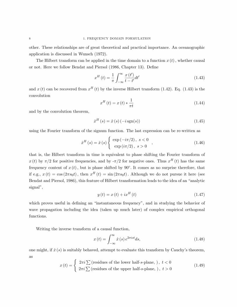
The Hilbert transform can be applied in the time domain to a function x (t) , whether causal
or not. Here we follow Bendat and Piersol (1986, Chapter 13). Define
xH (t) =1
π
Z ∞
−∞x (t0)t− t0
dt0 (1.43)
and x (t) can be recovered from xH (t) by the inverse Hilbert transform (1.42). Eq. (1.43) is the
convolution
xH (t) = x (t) ∗ 1πt
(1.44)
and by the convolution theorem,
xH (s) = x (s) (−i sgn(s)) (1.45)
using the Fourier transform of the signum function. The last expression can be re-written as
xH (s) = x (s)
(exp (−iπ/2) , s < 0exp (iπ/2) , s > 0
, (1.46)
that is, the Hilbert transform in time is equivalent to phase shifting the Fourier transform of
x (t) by π/2 for positive frequencies, and by -π/2 for negative ones. Thus xH (t) has the same
frequency content of x (t) , but is phase shifted by 90◦. It comes as no surprise therefore, thatif e.g., x (t) = cos (2πs0t) , then xH (t) = sin (2πs0t) . Although we do not pursue it here (see
Bendat and Piersol, 1986), this feature of Hilbert transformation leads to the idea of an “analytic
signal”,
y (t) = x (t) + ixH (t) (1.47)
which proves useful in defining an “instantaneous frequency”, and in studying the behavior of
wave propagation including the idea (taken up much later) of complex empirical orthogonal
functions.
Writing the inverse transform of a causal function,
x (t) =
Z ∞
−∞x (s) e2πistds, (1.48)
one might, if x (s) is suitably behaved, attempt to evaluate this transform by Cauchy’s theorem,
as
x (t) =
(2πi
P(residues of the lower half-s-plane, ) , t < 0
2πiP(residues of the upper half-s-plane, ) , t > 0
(1.49)

1. FOURIER TRANSFORMS AND DELTA FUNCTIONS 9
Since the first expression must vanish, if x (s) is a rational function, it cannot have any poles
in the lower-half-s−plane; this conclusion leads immediately so-called Wiener filter theory, andthe use of Wiener-Hopf methods.
1.3. Asymptotics. The gain of insight into the connections between a function and its
Fourier transform, and thus developing intuition, is a very powerful aid to interpreting the
real world. The scaling theorem, and its first-cousin, the uncertainty principle, are part of
that understanding. Another useful piece of information concerns the behavior of the Fourier
transform as |s|→∞. The classical result is the Riemann-Lebesgue Lemma. We can write
f (s) =
Z ∞
−∞f (t) e−2πistdt. (1.50)
where here, f (t) is assumed to satisfy the classical conditions for existence of the Fourier trans-
form pair. Let t0 = t− 1/ (2s) , (note the units are correct) then by a simple change of variablesrule,
f (s) = −Z ∞
−∞f
µt0 +
1
2s
¶e−2πist
0dt0 (1.51)
(exp (−iπ) = −1) and taking the average of these last two expressions, we have,¯f (s)
¯=
¯1
2
Z ∞
−∞f (t) e−2πistdt− 1
2
Z ∞
−∞f
µt+
1
2s
¶e−2πistdt
¯≤ 12
Z ∞
−∞
¯f (t)− f
µt+
1
2s
¶¯dt→ 0, as s→∞ (1.52)
because the difference between the two functions becomes arbitrarily small with increasing |s| .This result tells us that for classical functions, we are assured that for sufficiently large |s|
the Fourier transform will go to zero. It doesn’t however, tell us how fast it does go to zero.
A general theory is provided by Lighthill (1958), which he then builds into a complete analysis
system for asymptotic evaluation. He does this essentially by noting that functions such as
H (t) have Fourier transforms which for large |s| are dominated by the contribution from the
discontinuity in the first derivative, that is, for large s,H (s) → 1/s (compare to signum (t)).
Consideration of functions whose first derivatives are continuous, but whose second derivatives
are discontinuous, shows that they behave as 1/s2 for large |s| ; in general if the n− th derivativeis the first discontinuous one, then the function behaves asymptotically as 1/ |s|n. These are bothhandy rules for what happens and useful for evaluating integrals at large s (or large distances
if one is going from Fourier to physical space). Note that even the δ-function fits: its 0−thderivative is discontinuous (that is, the function itself), and its asymptotic behavior is 1/s0 =
constant; it does not decay at all as it violates the requirements of the Riemann-Lebesgue lemma.

10 1. FREQUENCY DOMAIN FORMULATION
2. Fourier Series and Time-Limited Functions
Suppose x (t) is periodic:
x (t) = x (t+ T ) (2.1)
Define the complex Fourier coefficients as
αn =1
T
Z T/2
−T/2x (t) exp
µ−2πintT
¶dt (2.2)
Then under very general conditions, one can represent x (t) in a Fourier Series:
x (t) =∞X
n=−∞αn exp
µ2πint
T
¶. (2.3)
Exercise. Show that x (t) can be written as a Fourier cosine and sine series:
x (t) =α02+
∞Xn=1
an cos
µ2πnt
T
¶+
∞Xn=1
bn sin
µ2πnt
T
¶and determine an, bn.
The Parseval Theorem for Fourier series is
1
T
Z T/2
−T/2x (t)2 dt =
∞Xn=−∞
|an|2 , (2.4)
and which follows immediately from the orthogonality of the complex exponentials over interval
T.
Exercise. Prove the Fourier Series versions of the shift, differentiation, scaling, and time-
reversal theorems.
Part of the utility of δ−functions is that they permit us to do a variety of calculations whichare not classically permitted. Consider for example, the Fourier transform of a periodic function,
e.g., any x (t) as in Eq. (2.3),
x (s) =
Z ∞
−∞
∞Xn=−∞
αne(2πint/T )e−2πistdt =
∞Xn=−∞
αnδ (s− n/T ) , (2.5)
ignoring all convergence issues. We thus have the nice result that a periodic function has a
Fourier transform; it has the property of vanishing except precisely at the usual Fourier series
frequencies where its value is a δ−function with amplitude equal to the complex Fourier seriescoefficient at that frequency.

2. FOURIER SERIES AND TIME-LIMITED FUNCTIONS 11
Suppose that instead,
x (t) = 0, |t| ≥ T/2 (2.6)
that is, x (t) is zero except in the finite interval −T/2 ≤ t ≤ T/2 (this is called a “time-limited”
function). The following elementary statement proves to be very useful. Write x (t) as a Fourier
series in |t| < T/2, and as zero elsewhere:
x (t) =
( P∞n=−∞ αn exp (2πint/T ) , |t| ≤ T/2
0, |t| > T/2(2.7)
where
αn =1
T
Z T/2
−T/2x (t) exp
µ−2πint
T
¶dt, (2.8)
as though it were actually periodic. Thus as defined, x (t) corresponds to some different, periodic
function, in the interval |t| ≤ T/2, and is zero outside. x (t) is perfectly defined by the special
sinusoids with frequency sn = n/T, n = 0,±1, ... ∞.The function x (t) isn’t periodic and so its Fourier transform can be computed in the ordinary
way,
x (s) =
Z T/2
−T/2x (t) e−2πistdt. (2.9)
and then,
x (t) =
Z ∞
−∞x (s) e2πistds. (2.10)
We observe that x (s) is defined at all frequencies s, on the continuum from 0 to ±∞. If we
look at the special frequencies s = sn = n/T, corresponding to the Fourier series representation
(2.7), we observe that
x (sn) = Tαn =1
1/Tαn. (2.11)
That is, the Fourier transform at the special Fourier series frequencies, differs from the corre-
sponding Fourier series coefficient by a constant multiplier. The second equality in (2.11) is
written specifically to show that the Fourier transform value x (s) , can be thought of as an
amplitude density per unit frequency, with the αn being separated by 1/T in frequency.
The information content of the representation of x (t) in (2.7) must be the same as in (2.10),
in the sense that x (t) is perfectly recovered from both. But there is a striking difference in
the apparent efficiency of the forms: the Fourier series requires values (a real and an imaginary
part) at a countable infinity of frequencies, while the Fourier transform requires a value on the
line continuum of all frequencies. One infers that the sole function of the infinite continuum
of values is to insure what is given by the second line of Eq. (2.7): that the function vanishes
outside |t| ≤ T/2. Some thought suggests the idea that one ought to be able to calculate the

12 1. FREQUENCY DOMAIN FORMULATION
Fourier transform at any frequency, from its values at the special Fourier series frequencies, and
this is both true, and a very powerful tool.
Let us compute the Fourier transform of x (t) , using the form (2.7):
x (s) =
Z T/2
−T/2
∞Xn=−∞
αn exp
µ2πint
T
¶exp (−2πist) dt (2.12)
and assuming we can interchange the order of integration and summation (we can),
x (s) = T∞X
n=−∞αnsin (πT (n/T − s))
πT (n/T − s)
=∞X
n=−∞x (sn)
sin (πT (n/T − s))
πT (n/T − s), (2.13)
using Eq. (2.11). Notice that as required x (s) = x (sn) = Tαn,when s = sn, but in between
these values, x (s) is a weighted (interpolated) linear combination of all of the Fourier Series
components.
Exercise. Prove by inverse Fourier transformation that any sum
x (s) =∞X
n=−∞βnsin (πT (n/T − s))
πT (n/T − s), (2.14)
where βn are arbitrary constants, corresponds to a function vanishing t > |T/2| , that is, atime-limited function.
The surprising import of (2.13) is that the Fourier transform of a time-limited function
can be perfectly reconstructed from a knowledge of its values at the Fourier series frequencies
alone. That means, in turn, that a knowledge of the countable infinity of Fourier coefficients
can reconstruct the original function exactly. Putting it slightly differently, there is no purpose
in computing a Fourier transform at frequency intervals closer than 1/T where T is either the
period, or the interval of observation.
3. The Sampling Theorem
We have seen that a time-limited function can be reconstructed from its Fourier coefficients.
The reader will probably have noticed that there is symmetry between frequency and time
domains. That is to say, apart from the assignment of the sign of the exponent of exp (2πist) ,
the s and t domains are essentially equivalent. For many purposes, it is helpful to use not t, s with
their physical connotations, but abstract symbols like q, r. Taking the lead from this inference,
3. THE SAMPLING THEOREM 13
let us interchange the t, s domains in the equations (2.6, 2.13), making the substitutions t →s, s→ t, T → 1/∆t, x (s)→ x (t) . We then have,
x (s) = 0, s ≥ 1/2∆t (3.1)
x (t) =∞X
m=−∞x (m∆t)
sin (π (m− t/∆t))
π (m− t/∆t)
=∞X
m=−∞x (m∆t)
sin ((π/∆t) (t−m∆t))
(π/∆t) (t−m∆t). (3.2)
This result asserts that a function bandlimited to the frequency interval |s| ≤ 1/2∆t (meaningthat its Fourier transform vanishes for all frequencies outside of this baseband) can be perfectly
reconstructed by samples of the function at the times m∆t. This result (3.1,3.2) is the famous
Shannon sampling theorem. As such, it is an interpolation statement. It can also be regarded
as a statement of information content: all of the information about the bandlimited continuous
time series is contained in the samples. This result is actually a remarkable one, as it asserts
that a continuous function with an uncountable infinity of points can be reconstructed from a
countable infinity of values.
Although one should never use (3.2) to interpolate data in practice (although so-called sinc
methods are used to do numerical integration of analytically-defined functions), the implications
of this rule are very important and can be stated in a variety of ways. In particular, let us write
a general bandlimiting form:
x (s) = 0, s ≥ sc (3.3)
If (3.3) is valid, it suffices to sample the function at uniform time intervals ∆t ≤ 1/2sc (Eq. 3.1is clearly then satisfied.).
Exercise. Let ∆t = 1. x (t) is measured at all times, and found to vanish, except for
t = m = 0, 1, 2, 3 and the values are [1, 2,−1,−1] . Calculate the values of x (t) at intervals∆t/10 from −5 ≤ t ≤ 5 and plot it. Find the Fourier transform of x (t) .
The consequence of the sampling theorem for discrete observations in time is that there is no
purpose in calculating the Fourier transform for frequencies larger in magnitude than 1/(2∆t).
Coupled with the result for time-limited functions, we conclude that all of the information about
a finite sequence of N observations at intervals ∆t and of duration, (N − 1)∆t is contained inthe baseband |s| ≤ 1/2∆t, at frequencies sn = n/ (N∆t) .

14 1. FREQUENCY DOMAIN FORMULATION
There is a theorem (owing to Paley and Wiener) that a time-limited function cannot be
band-limited, and vice-versa. One infers that a truly time-limited function must have a Fourier
transform with non-zero values extending to arbitrarily high frequencies, s. If such a function is
sampled, then some degree of aliasing is inevitable. For a truly band-limited function, one makes
the required interchange to show that it must actually extend with finite values to t = ±∞.
Some degree of aliasing of real signals is therefore inevitable. Nonetheless, such aliasing can
usually be rendered arbitrarily small and harmless; the need to be vigilant is, however, clear.
Irregular Sampling
Eq. (3.2) can be used as the starting point for a discussion of irregular sampling (Freeman,
1965). Suppose one of the samples, at time k∆t is missing, but one has instead, a sample at the
irregular time t = tk which can be anywhere. The question is whether the perfect reconstruction
can still be carried out by substituting the irregular sample for the missing regular one? The
answer is yes, and a new explicit interpolation formula can be constructed (Freeman, 1965).
Having replaced on regular sample with one irregular one, the same substitution can be carried
out indefinitely, and in the limit an arbitrary number of substitutions can take place. In the
limit an arbitrary number of the samples can occur in an arbitrarily small interval, which is
discncerting. Such a limit, however, depends delicately on the assumption of perfect data,
and the result would be extremely noise sensitive. Special cases of sampling theorems are of
interest as well, including so-called “interlaced-sampling” in which a large regular sampling
interval alternates with a smaller one (e.g., Bracewell, 2000).or half the samples are replaced by
measurements of the function derivatives. Some useful results about “jittered” sampling can be
seen in Moore and Thomson (1991), and Thomson and Robinson (1996); an application to an
ice core record is Wunsch (2000).
With real data, that is having measurement noise, a useful and general approach is to employ
the property (taken up below) that a Fourier series is a least-squares fit to the data. One can
then employ all of the machinery available in least-squares for determining resolving power and
uncertainty.
3.1. Tapering, Leakage, Etc. Suppose we have a continuous cosine x (t) = cos (2πp1t/T1) .
Then the true Fourier transform is
x (s) =1
2{δ (s− p1) + δ (s+ p1)} . (3.4)
If it is observed (continuously) over the interval −T/2 ≤ t ≤ T/2, then we have the Fourier
transform of
xΠ (t) = x (t)Π (t/T ) (3.5)

3. THE SAMPLING THEOREM 15
−5 −4 −3 −2 −1 0 1 2 3 4 5−0.4
−0.2
0
0.2
0.4
0.6
0.8
1
s
Figure 2. The function, sinc(sT ) = sin (πsT ) / (πsT ) , (solid line) which is
the Fourier transform of a pure exponential centered at that corresponding fre-
quency. Here T = 1. Notice that the function crosses zero whenever s = m,
which corresponds to the Fourier frequency separation. The main lobe has width
2, while successor lobes have width 1, with a decay rate only as fast as 1/ |s| . Thefunction sinc2 (s/2) (dotted line) decays as 1/ |s|2, but its main lobe appears, bythe scaling theorem, with twice the width of that of the sinc(s) function.
and which is found immediately to be
xΠ (s) =T
2
½sin (πT (s− p1))
(πT (s− p1))+sin (πT (s+ p1))
(πT (s+ p1))
¾(3.6)
The function
sinc (Ts) = sin (πTs) / (πTs) , (3.7)
plotted in Fig. (2), is ubiquitous in time series analysis and worth some study. Note that in
(3.6) there is a “main-lobe” of width 2/T (defined by the zero crossings) and with amplitude
maximum T . To each side of the main lobe, there is an infinite set of diminishing “sidelobes”
of width 1/T between zero crossings. Let us suppose that p1 in (3.4) is chosen to be one of
the special frequencies sn = n/T, T = N∆t, in particular, p1 = p/T. Then (3.6) is a sum
of two sinc functions centered at sp = ±p/T. A very important feature is that each of these
functions vanishes identically at all other special frequencies sn, n 6= p. If we confine ourselves,
as the inferences of the previous section imply, to computing the Fourier transform at only these
special frequencies, we would see only a large value T at s = sp and zero at every other such
frequency. (Note that if we convert to Fourier coefficients by division by 1/T, we obtain the

16 1. FREQUENCY DOMAIN FORMULATION
−10 −8 −6 −4 −2 0 2 4 6 8 10−0.4
−0.2
0
0.2
0.4
0.6
0.8
1
s
p=1.5, T=1
Figure 3. Interference pattern from a cosine, showing how contributions from
positive and negative frequencies add and subtract. Each vanishes at the central
frequency plus 1/T and at all other intervals separated by 1/T.
proper values.) The Fourier transform does not vanish for the continuum of frequencies s 6= sn,
but it could be obtained from the sampling theorem.
Now suppose that the cosine is no longer a Fourier harmonic of the record length. Then
computation of the Fourier transform at sn no longer produces a zero value; rather one obtains
a finite value from (3.6). In particular, if p1 lies halfway between two Fourier harmonics, n/T ≤p1 ≤ (n+ 1) /T , |x (sn)| , |x (sn+1)| will be approximately equal, and the absolute value of theremaining Fourier coefficients will diminish roughly as 1/ |n−m| . The words “approximately”and “roughly” are employed because there is another sinc function at the corresponding negative
frequencies, which generates finite values in the positive half of the s−axis. The analyst willnot be able to distinguish the result (a single pure Fourier frequency in between sn, sn+1) from
the possibility that there are two pure frequencies present at sn, sn+1. Thus we have what is
sometimes called “Rayleigh’s criterion”: that to separate, or “resolve” two pure sinusoids, at
frequencies p1, p2, their frequencies must differ by
|p1 − p2| ≥ 1
T, . (3.8)
or precisely by a Fourier harmonic; see Fig. 3. (The terminology and criterion originate in
spectroscopy where the main lobe of the sinc function is determined by the width, L, of a
physical slit playing the role of T.)
3. THE SAMPLING THEOREM 17
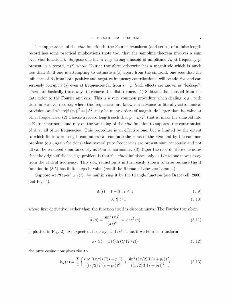
The appearance of the sinc function in the Fourier transform (and series) of a finite length
record has some practical implications (note too, that the sampling theorem involves a sum
over sinc functions). Suppose one has a very strong sinusoid of amplitude A, at frequency p,
present in a record, x (t) whose Fourier transform otherwise has a magnitude which is much
less than A. If one is attempting to estimate x (s) apart from the sinusoid, one sees that the
influence of A (from both positive and negative frequency contributions) will be additive and can
seriously corrupt x (s) even at frequencies far from s = p. Such effects are known as “leakage”.
There are basically three ways to remove this disturbance. (1) Subtract the sinusoid from the
data prior to the Fourier analysis. This is a very common procedure when dealing, e.g., with
tides in sealevel records, where the frequencies are known in advance to literally astronomical
precision, and where|x (sp)|2 ≈¯A2¯may be many orders of magnitude larger than its value at
other frequencies. (2) Choose a record length such that p = n/T ; that is, make the sinusoid into
a Fourier harmonic and rely on the vanishing of the sinc function to suppress the contribution
of A at all other frequencies. This procedure is an effective one, but is limited by the extent
to which finite word length computers can compute the zeros of the sinc and by the common
problem (e.g., again for tides) that several pure frequencies are present simultaneously and not
all can be rendered simultaneously as Fourier harmonics. (3) Taper the record. Here one notes
that the origin of the leakage problem is that the sinc diminishes only as 1/s as one moves away
from the central frequency. This slow reduction is in turn easily shown to arise because the Π
function in (3.5) has finite steps in value (recall the Riemann-Lebesgue Lemma.)
Suppose we “taper” xΠ (t) , by multiplying it by the triangle function (see Bracewell, 2000,
and Fig. 4),
Λ (t) = 1− |t| , t ≤ 1 (3.9)
= 0, |t| > 1 (3.10)
whose first derivative, rather than the function itself is discontinuous. The Fourier transform
Λ (s) =sin2 (πs)
(πs)2= sinc2 (s) (3.11)
is plotted in Fig. 2). As expected, it decays as 1/s2. Thus if we Fourier transform
xΛ (t) = x (t)Λ (t/ (T/2)) (3.12)
the pure cosine now gives rise to
xΛ (s) =T
2
½sin2 ((π/2)T (s− p1))
((π/2)T (s− p1))2 +
sin2 ((π/2)T (s+ p1))
((π/2)T (s+ p1))2
¾(3.13)

18 1. FREQUENCY DOMAIN FORMULATION
−2 −1.5 −1 −0.5 0 0.5 1 1.5 20
0.2
0.4
0.6
0.8
1
1.2
Figure 4. “Tophat”, or Π (t) (solid) and “triangle” or Λ (t/2). A finite record
can be regarded as the product x (t)Π (t/T ) , giving rise to the sinc pattern
response. If this finite record is tapered by multiplying it as x (t)Λ (t/ (2T )) , the
Fourier transform decays much more rapidly away from the central frequency of
any sinusoids present.
and hence the leakage diminishes much more rapidly, whether or not we have succeeded in
aligning the dominant cosine. A price exists however, which must be paid. Notice that the main
lobe of F (Λ (t/ (T/2))) has width not 2/T, but 4/T , that is, it is twice as wide as before, andthe resolution of the analysis would be 1/2 of what it was without tapering. Thus tapering the
record prior to Fourier analysis incurs a trade-off between leakage and resolution.
One might sensibly wonder if some intermediate function between the Π and Λ functions
exists so that one diminishes the leakage but without incurring a resolution penalty as large
as a factor of 2. The answer is “yes”; much effort has been made over the years to finding
tapers w (t), whose Fourier transforms W (s) have desirable properties. Such taper functions
are called “windows”. A common one tapers the ends by multiplying by half-cosines at either
end, cosines whose periods are a parameter of the analysis. Others go under the names of
Hamming, Hanning, Bartlett, etc. windows.
Later we will see that a sophisticated choice of windows leads to the elegant recent theory
of multitaper spectral analysis. At the moment, we will only make the observation that the Λ
taper and all other tapers, has the effect of throwing away data near the ends of the record, a
process which is always best regarded as perverse: one should not have to discard good data for
a good analysis procedure to work.

4. DISCRETE OBSERVATIONS 19
Although we have discussed leakage etc. for continuously sampled records, completely anal-
ogous results exist for sampled, finite, records. We leave further discussion to the references.
Exercise. Generate a pure cosine at frequency s1, and period T1 = 2π/s1. Numerically
compute its Fourier transform, and Fourier series coefficients, when the record length, T =integer
×T1, and when it is no longer an integer multiple of the period.
4. Discrete Observations
4.0.1. Sampling. The above results show that a band-limited function can be reconstructed
perfectly from an infinite set of (perfect) samples. Similarly, the Fourier transform of a time-
limited function can be reconstructed perfectly from an infinite number of (perfect) samples
(the Fourier Series frequencies). In observational practice, functions must be both band-limited
(one cannot store an infinite number of Fourier coefficients) and time-limited (one cannot store
an infinite number of samples). Before exploring what this all means, let us vary the problem
slightly. Suppose we have x (t) with Fourier transform x (s) and we sample x (t) at uniform
intervals m∆t without paying attention, initially, as to whether it is band-limited or not. What
is the relationship between the Fourier transform of the sampled function and that of x (t)? That
is, the above development does not tell us how to compute a Fourier transform from a set of
samples. One could use (3.2) , interpolating before computing the Fourier integral. As it turns
out, this is unnecessary.
We need some way to connect the sampled function with the underlying continuous values.
The δ−function proves to be the ideal representation. Eq. (2.13) produces a single sample attime tm. The quantity,
xIII (t) = x (t)∞X
n=−∞δ (t− n∆t) , (4.1)
vanishes except at t = q∆t for any integer q. The value associated with xIII (t) at that time
is found by integrating it in an infinitesimal interval −ε + q∆t ≤ t ≤ ε + q∆t and one finds
immediately that xIII (q∆t) = x (q∆t) . Note that all measurements are integrals over some time
interval, no matter how short (perhaps nanoseconds). Because the δ−function is infinitesimallybroad in time, the briefest of measurement integrals is adequate to assign a value.1.
Let us Fourier analyze xIII (t) , and evaluate it in two separate ways:
1δ−functions are meaningful only when integrated. Lighthill (1958) is a good primer on handling them. Muchof the book has been boiled down to the advice that, if in doubt about the meaning of an integral, “integrate by
parts”.

20 1. FREQUENCY DOMAIN FORMULATION
(I) Direct sum.
xIII (s) =
Z ∞
−∞x (t)
∞Xm=−∞
δ (t−m∆t) e−2πistdt
=∞X
m=−∞x (m∆t) e−2πism∆t. (4.2)
(II) By convolution.
xIII (s) = x (s) ∗ FÃ ∞Xm=−∞
δ (t−m∆t)
!. (4.3)
What is F ¡P∞m=−∞ δ (t−m∆t)
¢? We have, by direct integration,
FÃ ∞Xm=−∞
δ (t−m∆t)
!=
∞Xm=−∞
e−2πims∆t (4.4)
What function is this? The right-hand-side of (4.4) is clearly a Fourier series for a function
periodic with period 1/∆t, in s. I assert that the periodic function is ∆tδ (s) , and the reader
should confirm that computing the Fourier series representation of ∆tδ (s) in the s−domain,with period 1/∆t is exactly (4.4). But such a periodic δ−function can also be written2
∆t∞X
n=−∞δ (s− n/∆t) (4.5)
Thus (4.3) can be written
xIII (s) = x (s) ∗∆t∞X
n=−∞δ (s− n/∆t)
=
Z ∞
−∞x¡s0¢∆t
∞Xn=−∞
δ¡s− n/∆t− s0
¢ds0
= ∆t∞X
n=−∞x³s− n
∆t
´(4.6)
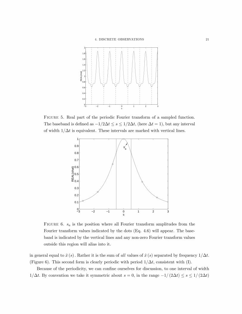
We now have two apparently very different representations of the Fourier transform of a
sampled function. (I) Asserts two important things. The Fourier transform can be computed as
the naive discretization of the complex exponentials (or cosines and sines if one prefers) times
the sample values. Equally important, the result is a periodic function with period 1/∆t. (Figure
5). Form (II) tells us that the value of the Fourier transform at a particular frequency s is not
2Bracewell (1978) gives a complete discussion of the behavior of these othewise peculiar functions. Note that
we are ignoring all questions of convergence, interchange of summation and integration etc. Everything can be
justified by appropriate limiting processes.
4. DISCRETE OBSERVATIONS 21
−3 −2 −1 0 1 2 30
0.2
0.4
0.6
0.8
1
1.2
1.4
1.6
1.8
2
s
RE
AL(
xhat
)
Figure 5. Real part of the periodic Fourier transform of a sampled function.
The baseband is defined as −1/2∆t ≤ s ≤ 1/2∆t, (here ∆t = 1), but any intervalof width 1/∆t is equivalent. These intervals are marked with vertical lines.
−3 −2 −1 0 1 2 30
0.1
0.2
0.3
0.4
0.5
0.6
0.7
0.8
0.9
1
s
RE
AL(
xhat
)
sa
Figure 6. sa is the position where all Fourier transform amplitudes from the
Fourier transform values indicated by the dots (Eq. 4.6) will appear. The base-
band is indicated by the vertical lines and any non-zero Fourier transform values
outside this region will alias into it.
in general equal to x (s) . Rather it is the sum of all values of x (s) separated by frequency 1/∆t.
(Figure 6). This second form is clearly periodic with period 1/∆t, consistent with (I).
Because of the periodicity, we can confine ourselves for discussion, to one interval of width
1/∆t. By convention we take it symmetric about s = 0, in the range −1/ (2∆t) ≤ s ≤ 1/ (2∆t)

22 1. FREQUENCY DOMAIN FORMULATION
which we call the baseband. We can now address the question of when xIII (s) in the baseband
will be equal to x (s)? The answer follows immediately from (4.6): if, and only if, x (s) vanishes
for s ≥ |1/2∆t| . That is, the Fourier transform of a sampled function will be the Fourier
transform of the original continuous function only if the original function is bandlimited and ∆t
is chosen to be small enough such that x (|s| > 1/∆t) = 0. We also see that there is no purposein computing xIII (s) outside the baseband: the function is perfectly periodic. We could use
the sampling theorem to interpolate our samples before Fourier transforming. But that would
produce a function which vanished outside the baseband–and we would be no wiser.
Suppose the original continuous function is
x (t) = A sin (2πs0t) . (4.7)
It follows immediately from the definition of the δ−function that
x (s) =i
2{δ (s+ s0)− δ (s− s0)} . (4.8)
If we choose ∆t < 1/2s0, we obtain the δ−functions in the baseband at the correct frequency.We ignore the δ−functions outside the baseband because we know them to be spurious. But
suppose we choose, either knowing what we are doing, or in ignorance, ∆t > 1/2s0. Then (4.6)
tells us that it will appear, spuriously, at
s = sa = s0 ±m/∆t, |sa| ≤ 1/2∆t (4.9)
thus determining m. The phenomenon of having a periodic function appear at an incorrect,
lower frequency, because of insufficiently rapid sampling, is called “aliasing” (and is familiar
through the stroboscope effect, as seen for example, in movies of turning wagon wheels).
5. Aliasing
Aliasing is an elementary result, and it is pervasive in science. Those who do not under-
stand it are condemned–as one can see in the literature–to sometimes foolish results (Wunsch,
2000). If one understands it, its presence can be benign. Consider for example, the TOPEX/-
POSEIDON satellite altimeter (e.g., Wunsch and Stammer, 1998), which samples a fixed position
on the earth with a return period (∆t) of 9.916 days=237.98 hours (h). The principle lunar semi-
diurnal tide (denoted M2) has a period of 12.42 hours. The spacecraft thus aliases the tide into
a frequency (from 4.9)
|sa| =¯
1
12.42h− n
237.98h
¯<
1
2× 237.98h . (5.1)

6. DISCRETE FOURIER ANALYSIS 23
To satisfy the inequality, one must choose n = 19, producing an alias frequency near sa =
1/61.6days, which is clearly observed in the data. (The TOPEX/POSEIDON orbit was very
carefully designed to avoid aliasing significant tidal lines (there are about 40 different frequencies
to be concerned about) into geophysically important frequencies such as those corresponding to
the mean (0 frequency), and the annual cycle (see Parke, et al., 1987)).
Exercise. Compute the alias period of the principal solar semidiurnal tide of period 12.00
hours as sampled by TOPEX/POSEIDON, and for both lunar and solar semidiurnal tides when
sampled by an altimeter in an orbit which returns to the same position every 35.00 days.
Exercise. The frequency of the so-called tropical year (based on passage of the sun through
the vernal equinox) is st = 1/365.244d. Suppose a temperature record is sampled at intervals
∆t = 365.25d. What is the apparent period of the tropical year signal? Suppose it is sampled
at ∆t = 365.00d (the “common year”). What then is the apparent period? What conclusion do
you draw?
Pure sinusoids are comparatively easily to deal with if aliased, as long as one knows their
origin. Inadequate sampling of functions with more complex Fourier transforms can be much
more pernicious. Consider the function shown in Figure 7a whose Fourier transform is shown
in Figure 7b. When sub-sampled as indicated, one obtains the Fourier transform in Fig. 7c. If
one was unaware of this effect, the result can be devastating for the interpretation. Once the
aliasing has occurred, there is no way to undo it. Aliasing is inexorable and unforgiving; we will
see it again when we study stochastic functions.
6. Discrete Fourier Analysis
The expression (4.2) shows that the Fourier transform of a discrete process is a function of
exp (−2πis) and hence is periodic with period 1 (or 1/∆t for general ∆t). A finite data lengthmeans that all of the information about it is contained in its values at the special frequencies
sn = n/T. If we define
z = e−2πis∆t (6.1)
the Fourier transform is
x (s) =
T/2Xm=−T/2
xmzm (6.2)
We will write this, somewhat inconsistently interchangeably, as x (s) , x¡e−2πis
¢, x (z) where the
two latter functions are identical; x (s) is clearly not the same function as x¡e−2πis
¢, but the
context should make clear what is intended. Notice that x (z) is just a polynomial in z, with

24 1. FREQUENCY DOMAIN FORMULATION
Figure 7. A function (a) with Fourier transform as in (b) is sampled as shown
at intervals ∆t, producing a corrupted (aliased) Fourier transform as shown in
(c). Modified after Press et al. (1992)
negative powers of z multiplying xn at negative times. That a Fourier transform (or series—which
differs only by a constant normalization) is a polynomial in exp (−2πis) proves to be a simple,but powerful idea.
Definition. We will use interchangeably the terminology “sequence”, “series” and “time se-
ries”, for the discrete function xm, whether it is discrete by definition, or is a sampled continuous
function. Any subscript implies a discrete value.
Consider for example, what happens if we multiply the Fourier transforms of xm, ym :
x (z) y (z) =
⎛⎝ T/2Xm=−T/2
xmzm
⎞⎠⎛⎝ T/2Xk=−T/2
ykzk
⎞⎠ =Xk
ÃXm
xmyk−m
!zk = h (z) . (6.3)
That is to say, the product of the two Fourier transforms is the Fourier transform of a new time
series,
hk =∞X
m=−∞xmyk−m, (6.4)
which is the rule for polynomial multiplication, and is a discrete generalization of convolution.
The infinite limits are a convenience–most often one or both time series vanishes beyond a
finite value.
More generally, the algebra of discrete Fourier transforms is the algebra of polynomials. We
could ignore the idea of a Fourier transform altogether and simply define a transform which

6. DISCRETE FOURIER ANALYSIS 25
Figure 8. Relationships between the complex z and s planes.
associates any sequence {xm} with the corresponding polynomial (6.2) , or formally
{xm}←→ Z (xm) ≡T/2X
m=−T/2xmz
m (6.5)
The operation of transforming a discrete sequence into a polynomial is called a z−transform.The z−transform coincides with the Fourier transform on the unit circle |z| = 1. If we regardz as a general complex variate, as the symbol is meant to suggest, we have at our disposal
the entire subject of complex functions to manipulate the Fourier transforms, as long as the
corresponding functions are finite on the unit circle. Fig. 8 shows how the complex s−plane,maps into the complex z−plane, the real line in the former, mapping into the unit circle, withthe upper half-s−plane becoming the interior of |z| = 1
There are many powerful results. One simple type is that any function analytic on the unit
circle corresponds to a Fourier transform of a sequence. For example, suppose
x (z) = Aeaz (6.6)
Because exp (az) is analytic everywhere for |z| < ∞, it has a convergent Taylor Series on the
unit circle
x (z) = A
µ1 + az + a2
z2
2!+ ....
¶(6.7)
and hence x0 = A,x1 = Aa, x2 = Aa2/2!, ...Note that xm = 0,m < 0. Such a sequence,
vanishing for negative m, is known as a “causal” one.

26 1. FREQUENCY DOMAIN FORMULATION
Exercise. Of what sequence is A sin (bz) the z−transform? What is the Fourier Series? Howabout,
x (z) =1
(1− az) (1− bz), a > 1, b < 1? (6.8)
This formalism permits us to define a “convolution inverse”. That is, given a sequence, xm,
can we find a sequence, bm, such that the discrete convolutionXk
bkxm−k =Xk
bm−kxk = δm0 (6.9)
where δm0 is the Kronecker delta (the discrete analogue of the Dirac δ)? To find bm, take the
z−transform of both sides, noting that Z (δm0) = 1, and we haveb (z) x (z) = 1 (6.10)
or
b (z) =1
x (z)(6.11)
But since x (z) is just a polynomial, we can find b (z) by simple polynomial division.
Example. Let xm = 0,m < 0, x0 = 1, x1 = 1/2, x2 = 1/4, xm = 1/8, ... What is its
convolution inverse? Z (xm) = 1 + z/2 + z2/4 + z3/8 + .... So
x (z) = 1 + z/2 + z2/4 + z3/8 + .... =1
1− (1/2) z (6.12)
so b (z) = 1− (1/2) z, with b0 = 1, b1 = −1/2, bm = 0, otherwise.Exercise. Confirm by direct convolution that the above bm is indeed the convolution inverse
of xm.
This idea leads to the extremely important field of “deconvolution”. Define
hm =∞X
n=−∞fngm−n =
∞Xn=−∞
gnfm−n. (6.13)
Define gm = 0,m < 0; that is, gm is causal. Then the second equality in (6.13) is
hm =∞Xn=0
gnfm−n, (6.14)
or writing it out,
hm = g0fm + g1fm−1 + g2fm−2 + .... (6.15)
If time t = m is regarded as the “present”, then gn operates only upon the present and earlier
(the past) values of fk; no future values of fm are required. Causal sequences gn appear, e.g.,
when one passes a signal, fk through a linear system which does not respond to the input before

6. DISCRETE FOURIER ANALYSIS 27
it occurs, that is the system is causal. Indeed, the notation gn has been used to suggest a Green
function. So-called real time filters are always of this form; they cannot operate on observations
which have not yet occurred.
In general, whether a z−transform requires positive, or negative powers of z (or both)
depends only upon the location of the singularities of the function relative to the unit circle. If
there are singularities in |z| < 1, a Laurent series is required for convergence on |z| = 1; if all
of the singularities occur for |z| > 1, a Taylor Series will be convergent and the function will
be causal. If both types of singularities are present, a Taylor-Laurent Series is required and the
sequence cannot be causal. When singularities exist on the unit circle itself, as with Fourier
transforms with singularities on the real s-axis one must decide through a limiting process what
the physics are.
Consider the problem of deconvolving hm in (6.15) from a knowledge of gn and hm, that is
one seeks fk. From the convolution theorem,
f (z) =h (z)
g (z)= h (z) a (z) . (6.16)
Could one find fk given only the past and present values of hm? Evidently, that requires a filter
a (z) which is also causal. Thus it cannot have any poles inside |z| < 1. The poles of a (z) are
evidently the zeros of g (z) and so the latter cannot have any zeros inside |z| < 1. Because g (z)is itself causal, if it is to have a (stable) causal inverse, it cannot have either poles or zeros inside
the unit circle. Such a sequence gm is called “minimum phase” and has a number of interesting
and useful properties (see e.g., Claerbout, 1985).
As one example, consider that it is possible to show that for any stationary, stochastic
process, xn, that one can always write it as
xn =∞Xk=0
anθn−k, a0 = 1
where an is minimum phase and θn is white noise, with < θ2n >= σ2θ. Let n be the present time.
Then one time-step in the future, one has
xn+1 = θn+1 +∞Xk=1
anθn−k.
Now at time n, θn+1 is completely unpredictable. Thus the best possible prediction is
xn+1 = 0 +∞Xk=1
anθn−k. (6.17)

28 1. FREQUENCY DOMAIN FORMULATION
with expected error,
< (xn+1 − xn+1)2 >=< θ2n >= σ2θ.
It is possible to show that this prediction, given an, is the best possible one; no other predictor
can have a smaller error than that given by the minimum phase operator an. If one wishes a
prediction q steps into the future, then it follows immediately that
xn+q =∞Xk=q
akθn+q−k,
< (xn+q − xn+q)2 >= σ2θ
qXk=0
a2k
which sensibly, has a monotonic growth with q. Notice that θk is determinable from xn and its
past values only, as the minimum phase property of ak guarantees the existence of the convolution
inverse filter, bk, such that,
θn =∞Xk=0
bkxn−k, b0 = 1.
Exercise. Consider a z−transformh (z) =
1
1− az(6.18)
and find the corresponding sequence hm when a→ 1 from above, and from below.
It is helpful, sometimes, to have an inverse transform operation which is more formal than
saying “read off the corresponding coefficient of zm). The inverse operator Z−1 is just the CauchyResidue Theorem
xm =1
2πi
I|z|=1
x (z)
zm+1dz. (6.19)
We leave all of the details to the textbooks (see especially, Claerbout, 1985).
The discrete analogue of cross-correlation involves two sequences xm, ym in the form
rτ =∞X
n=−∞xnyn+τ (6.20)
which is readily shown to be the convolution of ym with the time-reverse of xn. Thus by the
discrete time-reversal theorem,
F (rτ ) = r (s) = x (s)∗ y (s) . (6.21)
Equivalently,
r (z) = x
µ1
z
¶y (z) . (6.22)

6. DISCRETE FOURIER ANALYSIS 29
r¡z = e−2πis
¢= Φxy (s) is known as the cross-power spectrum of xn, yn.
If xn = yn, we have discrete autocorrelation, and
r (z) = x
µ1
z
¶x (z) . (6.23)
Notice that wherever x (z) has poles and zeros, x (1/z) will have corresponding zeros and poles.
r¡z = e−2πis
¢= Φxx (s) is known as the power spectrum of xn. Given any r (z) , the so-called
spectral factorization problem consists of finding two factors x (z), x (1/z) the first of which has
all poles and zeros outside |z| = 1, and the second having the corresponding zeros and poles
inside. The corresponding xm would be minimum phase.
Example. Let x0 = 1, x1 = 1/2, xn = 0, n 6= 0, 1. Then x (z) = 1+z/2, x (1/z) = 1+1/ (2z) ,
r (z) = (1 + 1/ (2z)) (1 + z/2) = 5/4 + 1/2 (z + 1/z) . Hence Φxx (s) = 5/4 + cos (2πs) .
Convolution as a Matrix Operation
Suppose fn, gn are both causal sequences. Then their convolution is
hm =∞Xn=0
gnfm−n (6.24)
or writing it out,
h0 = f0g0 (6.25)
h1 = f0g1 + f1g0
h2 = f0g2 + f1g1 + f2g0
...
which we can write in vector matrix form as⎡⎢⎢⎢⎢⎣h0
h1
h2
.
⎤⎥⎥⎥⎥⎦ =⎧⎪⎪⎪⎪⎨⎪⎪⎪⎪⎩
g0 0 0 0 . 0
g1 g0 0 0 . 0
g2 g1 g0 0 . 0
. . . . . .
⎫⎪⎪⎪⎪⎬⎪⎪⎪⎪⎭
⎡⎢⎢⎢⎢⎣f0
f1
f2
.
⎤⎥⎥⎥⎥⎦ ,or because convolution commutes, alternatively as⎡⎢⎢⎢⎢⎣
h0
h1
h2
.
⎤⎥⎥⎥⎥⎦ =⎧⎪⎪⎪⎪⎨⎪⎪⎪⎪⎩
f0 0 0 0 . 0
f1 f0 0 0 . 0
f2 f1 f0 0 . 0
. . . . . .
⎫⎪⎪⎪⎪⎬⎪⎪⎪⎪⎭
⎡⎢⎢⎢⎢⎣g0
g1
g2
.
⎤⎥⎥⎥⎥⎦ ,which can be written compactly as
h =Gf = Fg
30 1. FREQUENCY DOMAIN FORMULATION
where the notation should be obvious. Deconvolution then becomes, e.g.,
f =G−1h,
if the matrix inverse exists. These forms allow one to connect convolution, deconvolution and
signal processing generally to the matrix/vector tools discussed, e.g., in Wunsch (1996). Notice
that causality was not actually required to write convolution as a matrix operation; it was merely
convenient.
Starting in Discrete Space
One need not begin the discussion of Fourier transforms in continuous time, but can begin
directly with a discrete time series. Note that some processes are by nature discrete (e.g.,
population of a list of cities; stock market prices at closing-time each day) and there need
not be an underlying continuous process. But whether the process is discrete, or has been
discretized, the resulting Fourier transform is then periodic in frequency space. If the duration
of the record is finite (and it could be physically of limited lifetime, not just bounded by the
observation duration; for example, the width of the Atlantic Ocean is finite and limits the
wavenumber resolution of any analysis), then the resulting Fourier transform need be computed
only at a finite, countable number of points. Because the Fourier sines and cosines (or complex
exponentials) have the somewhat remarkable property of being exactly orthogonal not only when
integrated over the record length, but also of being exactly orthogonal when summed over the
same interval, one can do the entire analysis in discrete form.
Following the clear discussion in Hamming (1973, p. 510), let us for variety work with the
real sines and cosines. The development is slightly simpler if the number of data points, N, is
even, and we confine the discussion to that (if the number of data points is in practice odd,
one can modify what follows, or simply add a zero data point, or drop the last data point, to
reduce to the even number case). Define T = N∆t (notice that the basic time duration is not
(N − 1)∆t which is the true data duration, but has one extra time step. Then the sines and

6. DISCRETE FOURIER ANALYSIS 31
cosines have the following orthogonality properties:
N−1Xp=0
cos
µ2πk
Tp∆t
¶cos
µ2πm
Tp∆t
¶=
⎧⎪⎨⎪⎩0
N/2
N
,
k 6= m
k = m 6= 0, N/2
k = m = 0, N/2
(6.26)
N−1Xp=0
sin
µ2πk
Tp∆t
¶sin
µ2πm
Tp∆t
¶=
(0
N/2,
k 6= m
k = m 6= 0, N/2(6.27)
N−1Xp=0
cos
µ2πk
Tp∆t
¶sin
µ2πm
Tp∆t
¶= 0. (6.28)
Zero frequency, and the Nyquist frequency, are evidently special cases. Using these orthogonality
properties the expansion of an arbitrary sequence at data points m∆t proves to be:
xm =a02+
N/2−1Xk=1
ak cos
µ2πkm∆t
T
¶+
N/2−1Xk=1
bk sin
µ2πkm∆t
T
¶+aN/22
cos
µ2πNm∆t
2T
¶, (6.29)
where
ak =2
N
N−1Xp=0
xp cos
µ2πkp∆t
T
¶, k = 0, ..., N/2 (6.30)
bk =2
N
N−1Xp=0
xp sin
µ2πkp∆t
T
¶, k = 1, ...N/2− 1. (6.31)
The expression (6.29) separates the 0 and Nyquist frequencies and whose sine coefficients
always vanish; often for notational simplicity, we will assume that a0, aN vanish (removal of the
mean from a time series is almost always the first step in any case, and if there is significant
amplitude at the Nyquist frequency, one probably has significant aliasing going on.). Notice
that as expected, it requires N/2 + 1 values of ak and N/2 − 1 values of bk for a total of Nnumbers in the frequency domain, the same total numbers as in the time-domain.
Exercise. Write a computer code to implement (6.30,6.31) directly. Show numerically that
you can recover an arbitrary sequence xp.
The complex form of the Fourier series, would be
xm =
N/2Xk=−N/2
αke2πikm∆t/T (6.32)
αk =1
N
N−1Xp=0
xpe−2πikp∆t/T . (6.33)

32 1. FREQUENCY DOMAIN FORMULATION
This form follows from multiplying (6.32) by exp (−2πimr∆t/T ) , summing over m and noting
N−1Xm=0
e(k−r)2πim∆t/T =
(N, k = r¡
1− e(2πi(k−r))¢/¡1− e(2πi(k−r)/N)
¢= 0, k 6= r
. (6.34)
The last expression follows from the finite summation formula for geometric series,
N−1Xj=0
arj = a1− rN
1− r. (6.35)
The Parseval Relationship becomes
1
N
N−1Xm=0
x2m =
N/2Xk=−N/2
|αk|2 . (6.36)
The number of complex coefficients αk appears to involve 2 (N/2)+1 = N+1 complex numbers,
or 2N + 2 values, while the xm are only N real numbers. But it follows immediately that if xmare real, that α−k = α∗k, so that there is no new information in the negative index values, andα0, αN/2 = α−N/2 are both real so that the number of Fourier series values is identical. Notethat the Fourier transform values,x (sn) at the special frequencies sn = 2πn/T, are
x (sn) = Nαn, (6.37)
so that the Parseval relationship is modified to
N−1Xm=0
x2m =1
N
N/2Xk=−N/2
|x (sn)|2 . (6.38)
To avoid negative indexing issues, many software packages redefine the baseband to lie in the
positive range 0 ≤ k ≤ N with the negative frequencies appearing after the positive frequencies
(see, e.g., Press et al., 1992, p. 497). Supposing that we do this, the complex Fourier transform
can be written in vector/matrix form. Let zn = e−2πisnt, then⎡⎢⎢⎢⎢⎢⎢⎢⎢⎢⎣
x (s0)
x (s1)
x (s2)
.
x (sm)
.
⎤⎥⎥⎥⎥⎥⎥⎥⎥⎥⎦=
⎧⎪⎪⎪⎪⎪⎪⎪⎪⎪⎨⎪⎪⎪⎪⎪⎪⎪⎪⎪⎩
1 1 1 . 1 .
1 z11 z21 . zN1 .
1 z12 z22 . zN2 .
. . . . . .
1 z1m z2m . zNm .
. . . . . .
⎫⎪⎪⎪⎪⎪⎪⎪⎪⎪⎬⎪⎪⎪⎪⎪⎪⎪⎪⎪⎭
⎡⎢⎢⎢⎢⎢⎢⎢⎢⎢⎣
x0
x1
x2
.
xq
.
⎤⎥⎥⎥⎥⎥⎥⎥⎥⎥⎦. (6.39)
or,
x = Bx, (6.40)

7. IDENTITIES AND DIFFERENCE EQUATIONS 33
The inverse transform is thus just
x = B−1x, (6.41)
and the entire numerical operation can be thought of as a set of simultaneous equations, e.g.,
(6.41), for a set of unknowns x.
The relationship between the complex and the real forms of the Fourier series is found simply.
Let αn = cn + idn, then for real xm, (6.32) is,
xm =
N/2Xn=0
(cn + idn) (cos (2πnm/T ) + i sin (2πnm/T )) + (cn − idn) (cos (2πnm/T )− i sin (2πnm/T ))
=
N/2Xn=0
{2cn cos (2πnm/T )− 2dn sin (2πnm/T )} , (6.42)
so that,
an = 2Re (αn) , bn = −2 Im(αn) (6.43)
and when convenient, we can simply switch from one representation to the other.
Software that shifts the frequencies around has to be used carefully, as one typically re-
arranges the result to be physically meaningful (e.g., by placing negative frequency values in
a list preceding positive frequency values with zero frequency in the center). If an inverse
transform is to be implemented, one must shift back again to whatever convention the software
expects. Modern software computes Fourier transforms by a so-called fast Fourier transform
(FFT) algorithm, and not by the straightforward calculation of (6.30, 6.31). Various versions
of the FFT exist, but they all take account of the idea that many of the operations in these
coefficient calculations are done repeatedly, if the number, N of data points is not prime. I leave
the discussion of the FFT to the references (see also, Press et al., 1992), and will only say that
one should avoid prime N, and that for very large values of N, one must be concerned about
round-off errors propagating through the calculation.
Exercise. Consider a time series xm,−T/2 ≤ m ≤ T/2, sampled at intervals ∆t. It is desired
to interpolate to intervals ∆t/q, where q is a positive integer greater than 1. Show (numerically)
that an extremely fast method for doing so is to find x (s) , |s| ≤ 1/2∆t, using an FFT, to extendthe baseband with zeros to the new interval |s| ≤ q/ (2∆t) , and to inverse Fourier transform
back into the time domain. (This is called “Fourier interpolation” and is very useful.).
7. Identities and Difference Equations
Z−transform analogues exist for all of the theorems of ordinary Fourier transforms.
Exercise. Demonstrate:

34 1. FREQUENCY DOMAIN FORMULATION
The shift theorem: Z (xm−q) = zqx (z) .
The differentiation theorem: Z (xm − xm−1) = (1− z) x (z) . Discuss the influence of a dif-
ference operation like this has on the frequency content of x (s) .
The time-reversal theorem: Z (x−m) = x (1/z) .
These and related relationships render it simple to solve many difference equations. Consider
the difference equation
xm+1 − axm + bxm−1 = pm (7.1)
where pm is a known sequence and a, b are constant. To solve (7.1), take the z−transform of
both sides, using the shift theorem:
1
zx (z)− ax (z) + bzx (z) = p (z) (7.2)
and solving,
xp (z) =p (z)
(1/z − a+ bz). (7.3)
If pm = 0,m < 0 (making pm causal), then the solution (7.3) is both causal and stable only if
the zeros of (1/z − a+ z) lie outside |z| = 1.Exercise. Find the sequence corresponding to (7.3).
Eq. (7.3) is the particular solution to the difference equation. A second order difference
equation in general requires two boundary or initial conditions. Suppose x0, x1 are given. Then
in general we need a homogeneous solution to add to (7.3) to satisfy the two conditions. To
find a homogeneous solution, take xh (z) = Acm where A, c are constants. The requirement that
xh (z) be a solution to the homogeneous difference equation is evidently cm+1−acm+bcm−1 = 0or, c− a+ bc−1 = 0, which has two roots, c±. Thus the general solution is
xm = Z−1 (xp (z)) +A+cm+ +A−cm− (7.4)
where the two constants A± are available to satisfy the two initial conditions. Notice that theroots c± determine also the character of (7.3). This is a large subject, left at this point to thereferences.3
We should note that Box, Jenkins and Reisel (1994) solve similar equations without using
z−transforms. They instead define forward and backwards difference operators, e.g., B (xm) =xm−1,F (xm) = xm+1. It is readily shown that these operators obey the same algebraic rules as
do the z−transform, and hence the two approaches are equivalent.3The procedure of finding a particular and a homogeneous solution to the difference equation is wholly
analogous to the treatment of differential equations with constant coefficients.

9. FOURIER SERIES AS LEAST-SQUARES 35
Exercise. Evaluate (1− αB)−1 xm with |α| < 1.
8. Circular Convolution
There is one potentially puzzling feature of convolution for discrete sequences. Suppose one
has fm 6= 0,= 0, 1, 2, and is zero otherwise, and that gm 6= 0,m = 0, 1, 2, and is zero otherwise.
Then h = f ∗ g is,[h0,h1, h2,h3, h4, h5] = [f0g0, f0g1 + f1g0, f0g2 + f1g1 + f2g0, f1g2 + f2g0, f0g2], (8.1)
that is, is non-zero for 5 elements. But the product f (z) g (z) is the Fourier transform of only a 3-
term non-zero sequence. How can the two results be consistent? Note that f (z) , g (z) are Fourier
transforms of two sequences which are numerically indistinguishable from periodic ones with
period 2. Thus their product must also be a Fourier transform of a sequence indistinguishable
from periodic with period 2. f (z) g (z) is the Fourier transform of the convolution of two periodic
sequences fm, gm, not the ones in Eq. (8.1) that we have treated as being zero outside their
region of definition. Z−1³f (z) g (z)
´is the convolutionof two periodic sequences, and which
have “wrapped around” on each other–giving rise to their description as “circular convolution”.
To render circular convolution identical to Eq. (8.1), one should pad fm, gm with enough zeros
that their lengths are identical to that of hm before forming f (z) g (z) .
In a typical situation however, fm might be a simple filter, perhaps of length 10, and gm
might be a set of observations, perhaps of length 10,000. If one simply drops the five points on
each end for which the convolution overlaps the zeros “off-the-ends”, then the two results are
virtually identical. An extended discussion of this problem can be found in Press et al. (1992,
Section 12.4).
9. Fourier Series as Least-Squares
Discrete Fourier series (6.29) are an exact representation of the uniformly sampled function
if the number of basis functions (sines and cosines) are taken to equal the number, N, of data
points. Suppose we use a number of terms N 0 ≤ N, and seek a least-squares fit. That is, we
would like to minimize
J =T−1Xt=0
⎛⎝xt −[N 0/2]Xm=1
αme2πimt/T
⎞⎠⎛⎝xt −[N 0/2]Xm=1
αme2πimt/T
⎞⎠∗ . (9.1)
Taking the partial derivatives of J with respect to the am and setting to zero (generating the
least-squares normal equations), and invoking the orthogonality of the complex exponentials,
one finds that (1) the governing equations are perfectly diagonal and, (2) the am are given by

36 1. FREQUENCY DOMAIN FORMULATION
precisely (6.29, 6.30). Thus we can draw an important conclusion: a Fourier series, whether
partial or complete, represents a least-squares fit of the sines and cosines to a time series. Least-
squares is discussed at length in Wunsch (1996).
Exercise. Find the normal equations corresponding to (9.1) and show that the coefficient
matrix is diagonal.
Non-Uniform Sampling
This result (9.1) shows us one way to handle a non-uniformly spaced time series. Let x (t)
be sampled at arbitrary times tj . We can write
x (tj) =
[N 0/2]Xm=1
αme2πimtj/T + εj (9.2)
where εj represents an error to be minimized as
J =
jN−1Xj=0
ε2j =
jN−1Xj=0
⎛⎝x (tj)−[N 0/2]Xm=1
αne2πintj/T
⎞⎠⎛⎝x (tj)−[N 0/2]Xm=1
αme2πimtj/T
⎞⎠∗ , (9.3)
or the equivalent real form, and the normal equations found. The resulting coefficient matrix is
no longer diagonal, and one must solve the normal equations by Gaussian elimination or other
algorithm. If the record length and/or N 0 is not too large, this is a very effective procedure.For long records, the computation can become arduous. Fortunately, there exists a fast solution
method for the normal equations, generally called the Lomb-Scargle algorithm (discussed, e.g.,
by Press et al., 1992; an application to intermittent satellite sampling of the earth’s surface can
be seen in Wunsch (1991)). The complexities of the algorithm should not however, mask the
underlying idea, which is just least-squares.
Exercise. Generate a uniformly spaced time series, xt, by specifying the coefficients of its
Fourier series. Using the Fourier series, interpolate xt to generate an irregularly spaced set
of values of x (tj) . Using x (tj) and the normal equations derived from (9.3), determine the
Fourier components. Discuss their relationship to the known ones. Study what happens if the
x (tj) are corrupted by the addition of white noise. What happens if the observation times tjare corrupted by a white noise error? (“White noise” is defined below. For present purposes,
it can be understood as the output of an ordinary pseudo-random number generator on your
computer.)

10. STOCHASTIC PROCESSES 37
10. Stochastic Processes
Basic Probability
Probability theory is a large subject that has developed deep philosophical roots and cor-
responding firmly held differences of opinion about its interpretation. Some of these disputes
are very important, but for our purposes we will think of a probability density as a frequency
function (histogram) in the limit of an infinite number of trials of an experiment as the bin-sizes
go to zero. We assume that such a limit exists, and can be written for a random variable y, as
py (Y ) , where the subscript is the variable, and the argument Y is the values that y can take on
(distinguishing the physical variable, e.g. a temperature, from its numerical value). Sometimes
the subscript is dropped when the meaning is otherwise clear. The use of py (Y ) in practice
means that one is referring to the probability that y lies in the interval Y ≤ y ≤ Y + dY as
py (Y ) dY, that is, lying in some differential interval.
Two very useful probability densities are the uniform one over interval L
py (Y ) =1
L,−L2≤ Y ≤ L
2
= Π (Y/L) (10.1)
and the normal (orP),
py (Y ) =1√2πσ
e−(Y−m)2/(2σ2). (10.2)
The latter is also written G¡m,σ2
¢to denote a normal (Gaussian) density with mean m, and
variance σ2. Both (10.1,10.2) satisfy the necessary requirements, p ≥ 0, andZ ∞
−∞py (Y ) dY = 1. (10.3)
Define a bracket, < . > as the averaging operator with meaning of the integral over all
possible values of the argument times the probability density. Thus,
< y >=
Z ∞
−∞Y py (Y ) dY = m (10.4)
(the mean, or center of mass),
< y2 >=
Z ∞
−∞Y 2py (Y ) dY (10.5)
the second moment,
< (y− < y >)2 >=
Z ∞
−∞(Y − hyi)2 py (Y ) dY = σ2y (10.6)

38 1. FREQUENCY DOMAIN FORMULATION
the variance (second moment about the mean), etc. An important simple result is that if a is
constant (not random), then
hayi = a < y > . (10.7)
Let f (y) be any function of random variable, y. It follows from the frequency function
definition of the probability density, that
< f (y) >=
Z ∞
−∞f (Y ) py (Y ) dY. (10.8)
Eq. (10.7) is evidently a special case. Often it is useful to find the probability density of f
from that of y. We suppose that the function is invertible so that y (f) is known. Then the line
segment dY is mapped into a line-segment dF, by the rule,
dY =dy (F )
dFdF, (10.9)
we have immediately,
pg (F ) dF = py (Y (F ))dy (F )
dFdF. (10.10)
A special case would be f = ay + b, or y = (f − b) /a, dy (F ) /dF = 1/a, and thus
pg (F ) = py ((F − b) /a) /a. (10.11)
If this result is applied to (10.2), we have
pg (F ) =1√2πaσ
e−(F−b−ma)2/(2a2σ2) (10.12)
which is G¡b−ma, a2σ2
¢. Note that by choosing b = m/σ, a = 1/σ, that the new probability
density is G (0, 1)–a standard form that is the one usually tabulated.
If the derivative dy/dF should be zero or infinity, it implies that the mapping from y to f, or
from f to y is not unique, and some care is needed (the differentials are not uniquely mapped).
So consider G (0, 1) ,
py (Y ) =1√2π
e−Y2/2 (10.13)
and suppose ξ = y2. Then clearly the probability that ξ is less than zero is zero, and both ±ymap onto the same value of ξ indicated by,
dy
dξ=1
2y=
1
2√ξ
(10.14)
becoming infinite at ξ = 0. We can deduce therefore that,
pξ (X) =
(1√
2π√Xe−X/2, X ≥ 00, X < 0
. (10.15)

10. STOCHASTIC PROCESSES 39
multiplying by 2 to account for the negative Y contributions, too. Probability density (10.15)
is known as “chi-square with one degree-of-freedom” usually written χ21. “Degrees-of-freedom”
will be defined later. For future reference, note that ify2®= σ2, still with zero mean, then Eq.
(10.15) becomes
pξ (X) =
(1
σ√2π√Xe−X/(2σ
2), X ≥ 00, X < 0
(10.16)
It can become confusing to keep track of mapping functions g (y) which are not unique, and
a more systematic approach than used to find (10.15) is desirable. Introduce the “probability
distribution function”,
Py (Y ) =
Z Y
−∞py¡Y 0¢dY 0, (10.17)
which has the properties, dPy/dY ≥ 0, Py (∞) = 1, dPy/dY = py (Y ) . The interpretation of
Py (Y ) is as the probability that y is less than or equal to Y.
Then for the above case, with ξ = y2 and y being Gaussian,
Pξ (X) = probability thatn−√X ≤ Y ≤
√Xo= Py
³√X´− Py
³−√X´
(10.18)
=
Z √X
−∞1√2π
e−Y2/2dY −
Z −√X
−∞1√2π
e−Y2/2dY. (10.19)
And,
pξ (X) =d
dXPξ (X) =
d
dX
"Z √X
−∞1√2π
e−Y2/2dY −
Z −√X
−∞1√2π
e−Y2/2dY
#(10.20)
=
∙1√
2π√Xe−
12X
¸, X ≥ 0, (10.21)
identical to (10.15). “Leibniz’s rule” for differentiation of a variable upper bound of integra-
tion was used. This approach is quite general, as long as expressions such as (10.18) can be
constructed.
If there are two or more random variables, ξi, i = 1, 2., ...m we can discuss their “joint” or
“multi-variate probability densities”, pξ1ξ2... (Ξ1,Ξ2, ...Ξm) ; these are to be thought of as derived
from the limits of a counting experiment in which ξ1, ξ2.. are measured many times, and then
binned by the values observed. The limit, as the number of such observations goes to infinity
and as the bin size goes to zero, is supposed to exist.
If a joint probability density factors,
pξ1ξ2... (Ξ1,Ξ2, ...Ξm) = pξ1 (Ξ1) pξ2 (Ξ2) ...pξm(Ξm) (10.22)
then the ξi are said to be independent.

40 1. FREQUENCY DOMAIN FORMULATION
Example. The general, m−dimensional joint Gaussian probability density is defined as,
pξ1ξ2... (Ξ1,Ξ2, ...Ξm) = (10.23)
1
(2π)m/2 |R|1/2exp
µ−12(ξ −m)T R−1 (ξ −m)
¶.
Here ξ = [ξ1, ...ξm]T ,
R =
⎧⎪⎪⎪⎪⎪⎪⎪⎨⎪⎪⎪⎪⎪⎪⎪⎩
< (ξ1 −m1) (ξ1 −m1) > < (ξ1 −m1) (ξ2 −m2) > . . < (ξ1 −m1) (ξm −mm) >
< (ξ2 −m2) (ξ1 −m1) > < (ξ2 −m2) (ξ2 −m2) > . . < (ξ2 −m2) (ξm −mm) >
. . . . .
. . . . .
< (ξm −mm) (ξ1 −m1) > < (ξm −mm) (ξ2 −m2) > . . < (ξm −mm) (ξm −mm) >
⎫⎪⎪⎪⎪⎪⎪⎪⎬⎪⎪⎪⎪⎪⎪⎪⎭(10.24)
and |R| is the determinant. R can be written in a variety of ways including
R =
⎧⎪⎪⎪⎪⎪⎪⎪⎨⎪⎪⎪⎪⎪⎪⎪⎩
σ21 σ1σ2ρ12 . . σ1σmρ1m
σ2σ1ρ21 σ22 . . σ2σmρ2m
. . . . .
. . . . .
σmσ1ρm1 σmσ2ρm2 . . σ2m
⎫⎪⎪⎪⎪⎪⎪⎪⎬⎪⎪⎪⎪⎪⎪⎪⎭(10.25)
where the σ2i are the corresponding variances about the mean, and the ρij ≡< (ξi −mi)¡ξj −mj
¢>
/σiσj = ρji are called correlations (discussed below).
The important special case of two normal variables (“bivariate normal”) can be written as
pξ1ξ2 (Ξ1,Ξ2) = (10.26)
1
2πσ1σ2 (1− ρ2)1/2exp
(− 1
2 (1− ρ2)
Ã(Ξ1 −m1)
2
σ21− 2ρ (Ξ1 −m1) (Ξ2 −m2)
σ1σ2+(Ξ2 −m2)
2
σ22
!),
where ρ is defined as ρ =< (ξ1 −m1) (ξ2 −m2) > /σ1σ2, and taken up immediately below.
Other variants of (10.26) are possible.
Exercise. Show that if all ρij = 0, i 6= j, that (10.23) reduces to the product of m-univariate
normal distributions, hence showing that uncorrelated normal variates are also independent.
The joint expectations about the means (moments about the means) are, for two variates,
< ξ01ξ02 >=
Z ∞
−∞
Z ∞
−∞(Ξ1 −m1) (Ξ2 −m2) pξ1ξ2 (Ξ1,Ξ2) dΞ1dΞ2. (10.27)
We will use ξ0i to denote the variable with its mean removed. If ξ01, ξ
02 are independent, it follows
that <ξ01ξ02 >=< ξ01 >< ξ02 >= 0.

10. STOCHASTIC PROCESSES 41
If <ξ01ξ02 >6= 0, (suppressing the prime), then they are said to be “correlated” variables.
This implies that a knowledge of one of them provides some predictive capacity for the other.
We can use the idea of conditional probability, e.g., the probability that ξ2 takes on a particular
value (or range of values) Ξ2 given that ξ1 = Ξ1, which we write as
pξ2|ξ1 (Ξ2|Ξ1) . (10.28)
The textbooks all show that if ξ1, ξ2 are independent pξ2|ξ1 (Ξ2|Ξ1) = pξ2(Ξ2), that is, knowledge
of the value of ξ1 then contains no predictive information about ξ2.More generally, suppose that
we try to predict ξ2 from ξ1 in the form
ξ2 = aξ1 + ε (10.29)
where by definition ε is independent of ξ1. Forming < ξ2ξ1 >= a < ξ21 > + < εξ1 >= a < ξ21 >,
or
a =< ξ2ξ1 >
< ξ21 >, (10.30)
which would vanish if < ξ1ξ2 >= 0. Define the “correlation coefficient”
ρ =< ξ2ξ1 >
< ξ21 >1/2< ξ22 >
1/2. (10.31)
It is straightforward to show that |ρ| ≤ 1. (e.g., Priestley, p. 79) We have,
a = ρ< ξ22 >
1/2
< ξ21 >1/2
, (10.32)
and it follows that the fraction of the variance in ξ2 which is correlated with (predictable by
knowledge of ξ1) is just,
< ξ22 > ρ2 (10.33)
(the “correlated power”), and the part of the variance which is not predictable, is
< ξ22 >¡1− ρ2
¢(10.34)
which is the “uncorrelated power”. If ξ1, ξ2 are independent, they are uncorrelated; if they are
uncorrelated, they need not be independent.
Let there be m random variables ξ1, ...ξm, and suppose we define m new variables η1...ηmwhich are functions of the original variables. Conservation of area rules lead to the conclusion
that if the joint probability density of the ξi is pξ1ξ2...ξm (Ξ1,Ξ2, ...Ξm) , then the joint probability

42 1. FREQUENCY DOMAIN FORMULATION
density for the ηi is
pη1η2... (η1, η2, ..., ηm) = (10.35)
pξ1ξ2...ξm (Ξ1 (η1, ..., ηm) ,Ξ2 (η1, ..., ηm) , ...,Ξm (η1, ..., ηm))∂ (Ξ1,Ξ2, ...,Ξm)
∂ (η1, ..., ηm)
where∂ (Ξ1,Ξ2, ...,Ξm)
∂ (η1, ..., ηm)(10.36)
is the Jacobian of the transformation between the two sets of variables.
In one dimension, the most common and useful transformations are of the form η = aξ+b, a, b
constant. In most cases, we work with canonical probability densities, such that e.g., the mean
is zero, and the variance unity. The linear transformation, with Jacobian a or a−1 permits oneto use these standard densities for random variables with arbitrary means and variances (see Eq.
10.12). All the ideas concerning correlation, predictability and independence are generalizable
to more than two variables, through multiple and partial correlation studies, but these are left
to the references.
Example. Let x, y be two uncorrelated (and hence independent) Gaussian random variables
of zero mean and variance σ2. Define r =px2 + y2 and φ = tan−1 (y/x). We seek the joint
probability density for r, φ, and their univariate probability densities. The joint probability
density function is
px,y (X,Y ) =1
2πσexp
£− ¡X2 + Y 2¢/2σ2
¤.
The Jacobian of the transformation from (x, y) to (r, φ) is just r (Cartesian to polar coordinates).
Then the joint probability density of the new variables is
pr,φ (R,Φ) =R
2πσexp
£−R2/2σ2¤Integrating out the Φ variable over its entire range, −π ≤ φ ≤ π, (Φ doesn’t actually appear),
we have immediately,
pr (R) =R
σexp
¡−R2/2σ2¢ , (10.37)
and by inspection, it must be true that
pφ (Φ) =1
2π.
Thus the phase has a uniform distribution −π ≤ φ ≤ π, and the amplitude and phase are
uncorrelated with each other. Note that the probability density for r is called the “Rayleigh
distribution”.
Exercise. Find the mean and variance of a Rayleigh distributed variable.

10. STOCHASTIC PROCESSES 43
For time series work, the most importantm−dimensional probability density is the Gaussianor normal one (10.23). As the textbooks all show, the normal probability density has several
important special properties. One of them is that it is completely specified by its mean, m, and
covariance matrix, R =©< (ξi −mi)
¡ξj −mj
¢>ª, and that if any pair is uncorrelated, they
are also independent.
Adding Independent Variates. Characteristic Functions
A common problem is to determine the probability density of a sum of variates, e.g., ξ =
ξ1+ξ2+ .... Obtaining the probability density is best done by undertaking a seeming digression.
Consider an arbitrary random variable y with known probability density py (Y ) , and the function
g (y) = eiyt. By (10.8), its expected value is
φy (t) =< eiyt >=
Z ∞
−∞py (Y ) e
iY tdY, (10.38)
that is, up to the absence of a factor of 2π in the numerator of the exponential, the Fourier
transform of py (Y ) . This expected value is clearly a function of t (which should not be inter-
preted as time–its use is merely convention, as is the definition (10.38) without 2π where our
own convention would put it), which we will denote φy (t) , and which is called the “charac-
teristic function”. Now suppose we have two independent random variables y, x. Consider the
characteristic function for w = x+ y,
φw (t) =< ei(x+y)t >=< eixt >< eiyt >=
Z ∞
−∞eiXtpx (X) dX
Z ∞
−∞eiY tpy (Y ) dY, (10.39)
by independence. So
φw (t) = φx (t)φy (t) , (10.40)
that is to say, the product of two Fourier transforms. Because characteristic functions are defined
as Fourier transforms, it follows that the inverse transform is,
pw (W ) =1
2π
Z ∞
−∞φw (t) e
−iWtdt (10.41)
with the 1/2π being necessary because of its absence in the complex exponentials. But by the
convolution theorem (or its very slight re-derivation with this changed convention), we must
have
pw (W ) =
Z ∞
−∞px¡W 0¢ py ¡W −W 0¢ dW 0. (10.42)
The solution generalizes in an obvious way to the sum of an arbitrary number of independent
variables. If px = py, we have φw = φy (t)2 or for the sum of n such variables, φw (t) = φy (t)
n .
The characteristic function of the G (0, 1) Gaussian is readily found to be
φ (t) = e−t2/2, (10.43)

44 1. FREQUENCY DOMAIN FORMULATION
and thus the sum of two G (0, 1) variables would have a characteristic function, e−t2/2e−t2/2 =e−t2 , whose inverse transform is found to be
p (X) =1√2π√2e−X
2, (10.44)
that is to say another Gaussian of zero mean, but variance 2. It follows immediately from (10.43)
that a sum of n - G (0, 1) variables is a new G (0, n) variable. If X is instead the square of a
G¡0, σ2
¢variable, then Eq. (10.44) becomes
p (X) =1√
2π√2σ2
e−X2/σ2 (10.45)
One use of the characteristic function is in its relations to the moments of the corresponding
probability density. Let us suppose φ (t) has a convergent Taylor series about t = 0 :
φ (t) = 1 + tdφ (t)
dt
¯t=0
+t2
2!
d2φ (t)
dt2
¯t=0
+ .... (10.46)
But from (10.38) we can evaluate the successive derivatives:
dφ (t)
dt
¯t=0
=
Z ∞
−∞iY py (Y ) dY = im,
d2φ (t)
dt2
¯t=0
=
Z ∞
−∞(iY )2 py (Y ) dY = i2m2,
d3φ (t)
dt3
¯t=0
=
Z ∞
−∞(iY )3 py (Y ) dY = i3m3, (10.47)
d(n)φ (t)
dt(n)
¯¯t=0
=
Z ∞
−∞(iY )n py (Y ) dY = inmn,
Where mi are the successive moments of the probability density. Thus the successive moments
determine the terms of the Taylor series expansion in (10.46), and hence the probability density
itself. These results can be turned into a statement that a knowledge of all of the moments
mi of a random process is usually equivalent to knowledge of the complete probability density.
Conversely, knowledge of the characteristic function means that all of the moments are readily
generated from its derivatives evaluated at t = 0. (There are probability densities whose moments
are not finite, e.g., the Cauchy, and the argument fails for them.)
The characteristic function generalizes to multivariate probability densities by introduction
of Fourier transforms in several dimensions. Moment generation is achieved by using Taylor
series in several dimensions.
Central Limit Theorems (CLT)

10. STOCHASTIC PROCESSES 45
Consider the sum of n independent variables, ξi,
ξ = ξ1 + ....+ ξn (10.48)
all having the same mean, m1 and variance, σ21, and with the same, but arbitrary, probability
density, p1 (Ξ) . Then
< ξ >= m = nm1, < (ξ −m)2 >= σ2 = nσ21. (10.49)
Define the normalized variable
ξ =ξ −m
σ= ξ1 + ...+ ξn, ξi =
ξi −m1√nσ1
. (10.50)
Suppose that the characteristic function of ξi is φ1 (t) . Then by the shift and scaling theorems of
Fourier transforms, the characteristic function of ξi is φ1 (t) = φ1 (t/ (σ1√n)) exp (−im1t/ (σ1n)) .
Hence the characteristic function for ξ must be
φ (t) = φ1 (t)n =
he−im1t/(σ1
√n)φ1
¡t/¡σ1√n¢¢in
. (10.51)
Now φ1 (t) is evidently the characteristic function of a random variable with zero mean and
variance 1/n. Thus it must be true that (expanding in a Taylor Series), and using (10.46, 10.47),
e−im1t/(σ1√n)φ1
¡t/¡σ1√n¢¢= 1− t2
2n+O
µt3
σ1n3/2
¶. (10.52)
Thus to lowest order, (10.51) is
φ (t) =
µ1− t2
2n
¶n
. (10.53)
Taking the limit as n goes to infinity, and invoking L’Hôpital’s rule on the log of φ (t) , we have
φ (t)→ e−t2/2 (10.54)
Thus in this limit, the probability density for ξ is the inverse tranform of (10.54) and is
p (Ξ) =1√2π
e−Ξ2/2 (10.55)
that is, G (0, 1) . Or, using the scaling and shift theorems,
p (Ξ) =1√
nσ1√2π
e−(Ξ−nm1)2/(2
√nσ1). (10.56)
That is to say, we have shown that sums of large numbers of random variates have a tendency to
become Gaussian, whether or not the underlying probability densities are themselves Gaussian.
Result (10.56) is a special case of the so-called Central Limit Theorem (CLT), which can be
proved under much more general circumstances. There are clearly restrictions that could prevent
46 1. FREQUENCY DOMAIN FORMULATION
the limit (10.54) from being reached, but the CLT is often valid. Note the special case of a sample
average,
m =1
n
nXi=1
ξi, (10.57)
for which it follows immediately that m will have a probability density G¡m,σ2/n
¢.
Exercise. Suppose that p1 (Ξ) = 1/2 {δ (Ξ− 1) + δ (Ξ+ 1)} . Study the behavior of (10.51)as n→∞.What is the limiting probability density of the sum? Hint: use the binomial expansion
on (1/2n)¡eit + e−it
¢n.Stationarity
Consider a G¡0, σ2
¢time series xm such that Rnm =< xnxm > . Given the zero mean, and
specified R, we infer that the joint probability density px1x2...xk is (10.23) with m = 0. Let us
suppose that Rnm depends only upon the time difference τ = n−m, so that Rnm =< xnxn+τ >=
Rτ , independent of n. Such a time series is said to be “stationary in the wide sense”. If it is
also true that all statistics, including all higher moments such as < xnxmxp >, etc. only depend
upon the time interval among the time series elements, the time series is said to be “stationary”
or “stationary in the strict sense”. It is another nice property of normal variates that if they
are stationary in the wide-sense, they are stationary in the strict sense (most readily seen by
observing that in (10.23) R has all of its parameters dependent solely upon τ , and not upon
the absolute time. Hence, the probability density depends only upon τ , as does any statistical
property derived from it. The theory for stationary time series is highly developed, and it is
commonly assumed that one is dealing in nature with stationary processes, but one must be
alert to the potential failure of the assumption.
Sample Estimates
In working with random variables, it is very important to distinguish between a theoretical
value, e.g., the true average, written < y >, or m, and the sample value, such as the sample
average, written as either < y >N or m, where the N subscript indicates that it was based upon
N observations. We use a tilde, ~, to mark an estimate of a variable; estimates are themselves
always random variables (e.g. m) where the parameter itself, m is not.
The usual sample average is
m =< y >N=1
N
NXi=1
yi. (10.58)
A useful property of a sample mean (or estimator of the mean) is that it’s own expected value
should be equal to the true value (this is not always true, and as will be seen, it is not always

10. STOCHASTIC PROCESSES 47
completely desirable.) For example,
< m >=1
N
NXi=1
< yi >=1
N
NXi=1
m = m (10.59)
Such an estimator is said to be unbiased. (If we could average N experimental values in M
separate experiments, the average of the sample averages would be expected to be the true
average.)
It helps to know what is the scatter of an estimate about its true value, so consider the
variance:
< (m−m)2 >=<
"1
N
NXi=1
yi −m
#2>=<
"1
N
NXi=1
(yi −m)
#2> (10.60)
=1
N2
NXi=1
< (yi −m)2 >=Nσ2
N2=
σ2
N(10.61)
so that the standard deviation of a sample mean about the true mean is σ/√N, which is the
famous “square-root of N” rule.
Now consider the sample variance:
σ2 =1
N
NXi=1
(yi − m)2 (10.62)
computed as the sample variance about the sample mean. A little algebra (left as an exercise),
shows that,
< σ2 >=N − 1N
σ2 6= σ2 (10.63)
that is to say, the sample variance is biassed (although it is asymptotically unbiased as N →∞).The bias is readily removed by re-defining
σ2 =1
N − 1NXi=1
(yi − m)2. (10.64)
The origin of the bias in this case is that in (10.62) the N terms being averaged are not indepen-
dent of each other; rather since the sum is taken over the values of yi−m, the last term could be
predicted from the preceding N−1 of them by the requirement that the sample average actuallyis m. Consequently there are only N −1 independent terms (N −1 “degrees-of-freedom”) in thesum.
Consistent Estimators
Data are used to estimate various properties characterizing the statistical population from
which the observation come. For example, the sample mean (10.58), is intended to be a good

48 1. FREQUENCY DOMAIN FORMULATION
estimate of the true average m, from which the data were drawn. Many other properties are
estimated, including the variance and the power density spectrum (defined below). Any estimate
of a property has to be examined for at least two desirable properties: (1) that the average value
of the estimate should be the true value (for an unbiased estimate), at least as the number
of samples becomes large, and (2) that as the number of samples becomes large, the variance
of the sample about its mean value (which one might hope is the true value) ought to go to
zero. Estimators with these two properties are said to be “consistent”. Sometimes however,
demanding an unbiased estimator greatly increases the variance of the estimate, and one may
deliberately permit a bias if the variance can thereby be reduced. The sample mean was shown
above to be unbiased, and by (10.60) its variance about the true value diminishes with N ; hence
it is a consistent estimator. One can also show that σ2 in the form (10.64) is also a consistent
estimator as is the original definition, in the asymptotic limit.
A useful idea in this context is the Chebyschev inequality. Let ξ be any random variable
with true mean m, variance σ2 and second moment < ξ2 >= m2 (that is not taken about the
mean). Then
m2 =
Z ∞
−∞Ξ2p (Ξ) dΞ ≥
µZ −δ
−∞+
Z ∞
δ
¶Ξ2p (Ξ) dΞ (10.65)
≥ δ2µZ −δ
−∞+
Z ∞
δ
¶p (Ξ) dΞ (10.66)
since ξ2 is always greater than or equal to δ2 in the integral. So we have the weak inequalityZ|ξ|>δ
p (Ξ) dΞ ≤ m2
δ2, (10.67)
which we can read as “the probability that |ξ| > δ is less than or equal to m2/δ2.” If we replace
ξ by ξ −m, and then m2 = σ2, we have
prob {|ξ −m| ≥ δ} ≤ σ2
δ2(10.68)
where “prob” denotes “the probability that”. The sense of the inequality can be inverted to
prob {|ξ −m| ≤ δ} ≥ 1− σ2
δ2, (10.69)
which is the Chebyschev inequality. These inequalities in turn lead to the important idea of
“convergence in probability”. ξk (where k is a parameter) is said to converge in probability to c,
as k → ∞, if prob{|ξk − c| ≥ δ} → 0. This is convergence that is “almost surely”, written a.s.,
and differs from ordinary mathematical convergence in being a statement that deviation from
the asymptotic value becomes extremely improbable, but not impossible, in the limit.
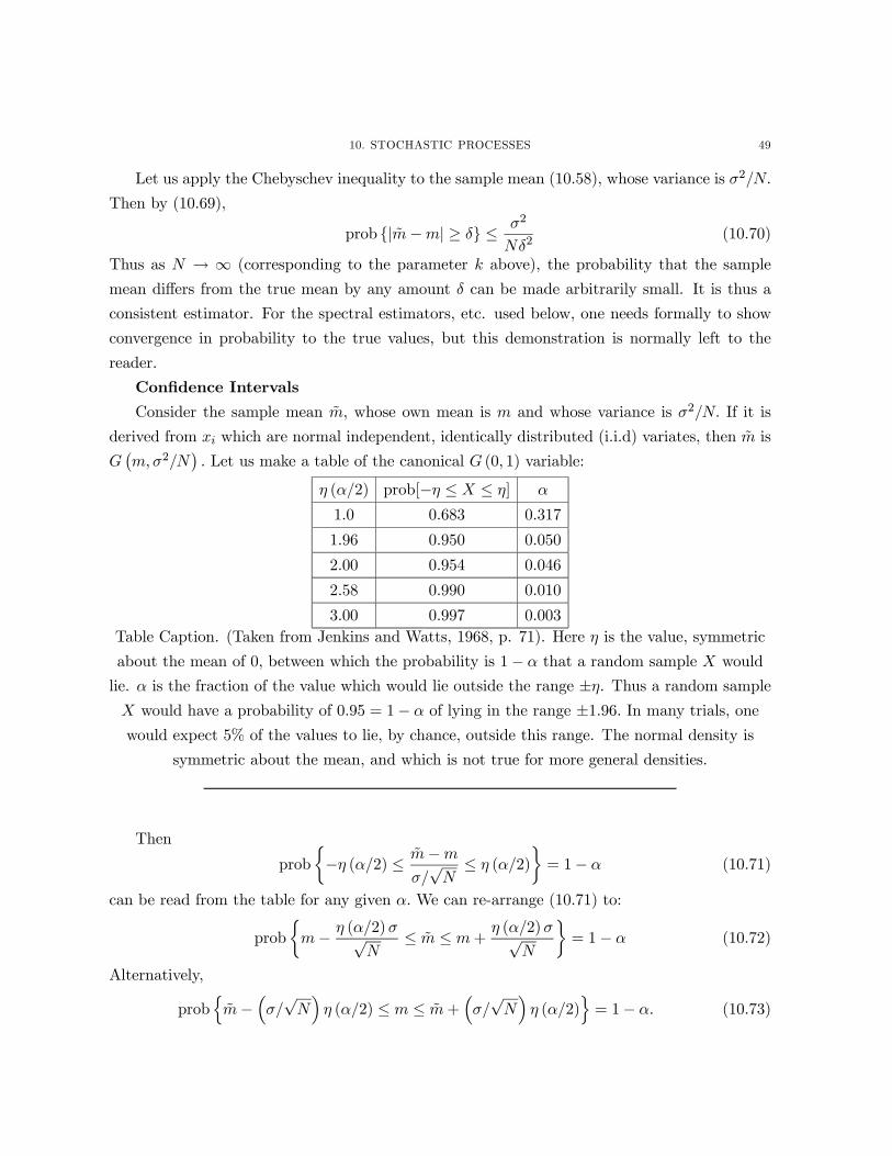
10. STOCHASTIC PROCESSES 49
Let us apply the Chebyschev inequality to the sample mean (10.58), whose variance is σ2/N.
Then by (10.69),
prob {|m−m| ≥ δ} ≤ σ2
Nδ2(10.70)
Thus as N → ∞ (corresponding to the parameter k above), the probability that the sample
mean differs from the true mean by any amount δ can be made arbitrarily small. It is thus a
consistent estimator. For the spectral estimators, etc. used below, one needs formally to show
convergence in probability to the true values, but this demonstration is normally left to the
reader.
Confidence Intervals
Consider the sample mean m, whose own mean is m and whose variance is σ2/N. If it is
derived from xi which are normal independent, identically distributed (i.i.d) variates, then m is
G¡m,σ2/N
¢. Let us make a table of the canonical G (0, 1) variable:
η (α/2) prob[−η ≤ X ≤ η] α
1.0 0.683 0.317
1.96 0.950 0.050
2.00 0.954 0.046
2.58 0.990 0.010
3.00 0.997 0.003Table Caption. (Taken from Jenkins and Watts, 1968, p. 71). Here η is the value, symmetric
about the mean of 0, between which the probability is 1− α that a random sample X would
lie. α is the fraction of the value which would lie outside the range ±η. Thus a random sample
X would have a probability of 0.95 = 1− α of lying in the range ±1.96. In many trials, onewould expect 5% of the values to lie, by chance, outside this range. The normal density is
symmetric about the mean, and which is not true for more general densities.
Then
prob½−η (α/2) ≤ m−m
σ/√N≤ η (α/2)
¾= 1− α (10.71)
can be read from the table for any given α. We can re-arrange (10.71) to:
prob½m− η (α/2)σ√
N≤ m ≤ m+
η (α/2)σ√N
¾= 1− α (10.72)
Alternatively,
probnm−
³σ/√N´η (α/2) ≤ m ≤ m+
³σ/√N´η (α/2)
o= 1− α. (10.73)

50 1. FREQUENCY DOMAIN FORMULATION
0 1 2 3 4 5 6 7 8 9 100
0.2
0.4
0.6
0.8
1
1.2
1.4
1.6
1.8
ν =1
2
4
Figure 9. Probability density for χ2ν , ν = 1, ..., 4. Note growth of long positive
tail as ν increases. m = ν, and σ2 = 2ν. For large ν, χ2ν approaches a normal
probability density. The cases ν = 1, 2 are exceptional in having their maximum
at 0.
This last form is the most useful one: suppose to be specific that α = .05. Then for a sample
mean m obtained from a random variate having variance σ2, the probability is 0.95 that the
true value, m, lies in the interval m±ση (.05/2) . This interval is said to be a 1−α% confidence
interval (here a 95% confidence interval). It clearly diminishes to zero as N →∞.
Consider now a non-symmetric probability density. One that proves very useful to us is the
so-called χ2ν (chi-square with ν degrees-of-freedom),
pξ (X) =1
2ν/2Γ (ν/2)Xν/2−1 exp (−X/2) , X > 0 (10.74)
= 0, X ≤ 0
whose mean is ν, and variance is 2ν. (This probability density describes a variable x =Pν1 ξ
2i ,
where the ξi are independent, G (0, 1) .) It is plotted in fig. 9 for 1 ≤ ν ≤ 4. For present
purposes, we note only that the probability density is non-symmetric about its mean, having a
long tail toward high positive values. Consider the tail at the low end containing a fraction a/2
of the values from a set of random trials, and denote the value X below which this tail falls as
η− (α/2) . Correspondingly, the tail at the high end occupying α/2 of the trial results is to lie
to the right of X = η+ (α/2) . Suppose now that we have a variable ξ which has been estimated

10. STOCHASTIC PROCESSES 51
as ξ and which is thought to be distributed in χ2ν with mean ν and variance 2ν. Then
probnη− (α/2) ≤ ξ ≤ η+ (α/2)
o= 1− α. (10.75)
To employ this in a practical example, consider the sample variance σ2 (10.64) constructed from
N idenditically distributed variables, which are G¡m,σ2
¢. It is easy to show (sketched out
below) that (N −1)σ2/σ2 will be a χ2ν variable with ν = N −1 (it’s expected value is N −1, andits variance is 2(N − 1)). Then setting ξ = (N − 1)σ2/σ2 in (10.75) and rearranging, we obtain
prob½σ2 (N − 1)η+ (α/2)
≤ σ2 ≤ σ2 (N − 1)η− (α/2)
¾= 1− α (10.76)
and the true variance would like between these two (unequal) bounds about σ2. Because η− < η+,
the upper limit of the α% confidence limit will be further above σ2 than the lower limit will be
below (for ν > 2). η± are tabulated in various statistics books or can be calculated from varioussoftware packages. (It is sometimes useful to have the χ2ν distribution for the sum, ξ, of squared
zero-mean Gaussian variates of variance σ2, or:
pξ (X) =1
σ22ν/2Γ (ν/2)
µX
σ2
¶ν/2−1exp
¡−X/¡2σ2
¢¢, X ≥ 0 (10.77)
= 0, X < 0.)
In examining the form (10.73), one might object that σ2 is not likely to be known. This
led Gosset (writing under the famous pseudonym of “Student”) to show that he could find the
probability density of the variable TN−1 =√N (m−m) /σ and which is not dependent upon σ.
The resulting probability density is called Student’s t−distribution. We leave its discussion tothe references (see, e.g., Cramér, 1946, Section 18.2).
White Noise
A white noise process is a stationary time series (sequence) with a uniform in time variance,
zero mean, and in which knowledge of the value at one time θm carries no information about
its value at any other time, including the immediately preceding and following times. That is,
< θmθm0 >= σ2θδmm0 . A sequence of coin flips is such a process. The general terminology is that
these are independent identically distributed variables (or an i.i.d). Often, we will assume that
the values are normally distributed, as in (10.2) with m = 0.

52 1. FREQUENCY DOMAIN FORMULATION
White noise is the simplest possible stochastic process. Let us therefore consider its Fourier
transform or series using the real form (6.29-6.31). The coefficients are
ak =2
N
N−1Xp=0
θp cos
µ2πkp∆t
T
¶, k = 0, ..., N/2, (10.78)
bk =2
N
N−1Xp=0
θp sin
µ2πkp∆t
T
¶, k = 1, ..., N/2− 1. (10.79)
It follows immediately that,
< ak >=< bk >= 0
< a2k >=4
N2<
N−1Xp=0
θp cos
µ2πkp∆t
T
¶N−1Xr=0
θr cos
µ2πkp∆t
T
¶>
=4
N2
XX< θpθr > cos
µ2πkp∆t
T
¶cos
µ2πkr∆t
T
¶=
4
N2
XXδprσ
2θ cos
µ2πkp∆t
T
¶cos
µ2πkp∆t
T
¶=2
Nσ2θ (10.80)
by (6.30). Similarly,
< b2k >=2
Nσ2θ (10.81)
< anbk >= 0 (10.82)
< akan >=< bkbn >=2
Nδknσ
2θ, (10.83)
omitting the zero and Nyquist frequencies. For these frequencies,
< a20 >=< a2N/2 >=4
N. (10.84)
To say this in words: the Fourier transform of a white noise process has zero mean and is
uncorrelated from one frequency to another; the sine and cosine amplitudes are uncorrelated
with each other at all frequencies, and the variance of the sine and cosine components is uniform
with frequency. If the θm are normally distributed, G¡0, σ2θ
¢then it follows immediately that
ak, bk are also normally distributed G¡0, 2σ2θ/N
¢. The Parseval relationship requires
1
N
N−1Xm=0
θ2m =a204+1
2
N/2−1Xm=1
¡a2m + b2n
¢+
a2N/2
4, (10.85)
10. STOCHASTIC PROCESSES 53
here including the mean and Nyquist frequencies. (The true mean is zero, but the actual sample
mean will not be, although it is often set to zero for numerical reasons. Doing so, means that
only N − 1 of the terms on the left in (10.85) would then be independent.) To check this lastequation, we can see if it holds on the average:
1
N
N−1Xm=0
< θ2m >?=
< a20 >
4+1
2
N/2−1Xn=1
<¡a2n + b2n
¢> +
< a2/2N/2 >
4, or,
σ2θ?=
σ2θN+1
2
N/2−1Xn=1
µ2
N+2
N
¶σ2θ +
σ2θN=
σ2θN+1
2
µN
2− 1¶4
Nσ2θ +
σ2θN= σ2θ, (10.86)
as required.
As the record length grows, the numberN, of Fourier coefficients grows linearly, but the mean
square power (1/N)PN−1
m=0 θ2m in (10.85) remains fixed, independent of N. Thus the expected
value of any a2n + b2n is reduced by the factor 1/N to compensate for their growing population.
If one computes the phase of the Fourier series as
φn = tan−1 (bn/an) (10.87)
it is readily seen that φn has a uniform probability density
pφ (Φ) =1
2π. (10.88)
(To see this algebraically, we recognize that if θm are G¡0, σ2θ
¢, an, bn are uncorrelated Gaussian
variables distributed G¡0, σ2θ/2N
¢and hence they are also independent. Because they are
independent, their joint probability density is the product of their identical probability densities:
pan,bn (Ξ1,Ξ2) = pan (Ξ1) pbn (Ξ2) = (10.89)
1
2π¡σ2θ/2N
¢ exp ¡−Ξ21/ ¡σ2θ/2N¢¢ exp ¡−Ξ22/ ¡σ2θ/2N¢¢
We can thus conclude that there is no information content in the phase of a white noise
process. What then is the probability density for a2n, b2n and a2n + b2n? The probability densities
for the first two must be identical, and are thus the densities for the square of a normal variate
with 0 mean and variance σ2θ/2N. Let us use normalized variables so that they have unit variance,
i.e., consider a0n = an/³σθ/√2N´, b0n = bn/
³σθ/√2N´each of which will be G(0, 1). Using the
rule for change of variable we find that,
pa02n (X) = pb02n (X) =X−1/2√2π
exp (−X/2) (10.90)
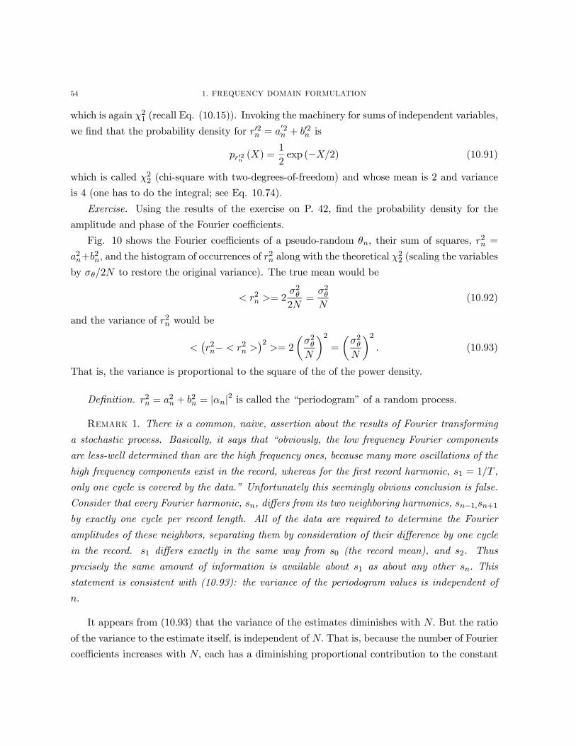
54 1. FREQUENCY DOMAIN FORMULATION
which is again χ21 (recall Eq. (10.15)). Invoking the machinery for sums of independent variables,
we find that the probability density for r02n = a02n + b02n is
pr02n (X) =1
2exp (−X/2) (10.91)
which is called χ22 (chi-square with two-degrees-of-freedom) and whose mean is 2 and variance
is 4 (one has to do the integral; see Eq. 10.74).
Exercise. Using the results of the exercise on P. 42, find the probability density for the
amplitude and phase of the Fourier coefficients.
Fig. 10 shows the Fourier coefficients of a pseudo-random θn, their sum of squares, r2n =
a2n+b2n, and the histogram of occurrences of r
2n along with the theoretical χ
22 (scaling the variables
by σθ/2N to restore the original variance). The true mean would be
< r2n >= 2σ2θ2N
=σ2θN
(10.92)
and the variance of r2n would be
<¡r2n− < r2n >
¢2>= 2
µσ2θN
¶2=
µσ2θN
¶2. (10.93)
That is, the variance is proportional to the square of the of the power density.
Definition. r2n = a2n + b2n = |αn|2 is called the “periodogram” of a random process.
Remark 1. There is a common, naive, assertion about the results of Fourier transforming
a stochastic process. Basically, it says that “obviously, the low frequency Fourier components
are less-well determined than are the high frequency ones, because many more oscillations of the
high frequency components exist in the record, whereas for the first record harmonic, s1 = 1/T ,
only one cycle is covered by the data.” Unfortunately this seemingly obvious conclusion is false.
Consider that every Fourier harmonic, sn, differs from its two neighboring harmonics, sn−1,sn+1by exactly one cycle per record length. All of the data are required to determine the Fourier
amplitudes of these neighbors, separating them by consideration of their difference by one cycle
in the record. s1 differs exactly in the same way from s0 (the record mean), and s2. Thus
precisely the same amount of information is available about s1 as about any other sn. This
statement is consistent with (10.93): the variance of the periodogram values is independent of
n.
It appears from (10.93) that the variance of the estimates diminishes with N. But the ratio
of the variance to the estimate itself, is independent of N. That is, because the number of Fourier
coefficients increases with N, each has a diminishing proportional contribution to the constant

11. SPECTRAL ESTIMATION 55
0 500 1000 1500 2000−4
−2
0
2
4(a)
0 0.1 0.2 0.3 0.4 0.50
0.005
0.01
0.015
FREQUENCY. CPD
|yha
t(s)
|2
(b)
10−4
10−2
100
0
1
2
3
4
5
6x 10
−3
FREQUENCY. CPD
s.*a
bs(y
hat)
2
(c)
0 0.005 0.01 0.0150
50
100
150
200
250
NU
MB
ER
abs(yhat).2
(d)
Figure 10. (a) 2048 numbers from a pseudo-random generator. These approxi-
mate a white noise process. (b) Linear scale periodogram of the values in (a). (c)
Semi-logarithmic scale plot of s |αn|2 in which the multiplication by s compen-
sates for the logarithmic squeezing of the frequencies at the high end. Notice the
visual impression that energy increases with increasing frequency–an artifact
of the plotting method. (d) 30 bin histogram of the values |αn|2 which shouldand do approximate a χ22 variate. The mean (dashed) and median (solid) values
are shown. There is evidently a much greater chance of a value far larger than
the mean to occur than there is for a much smaller one to occur, owing to the
limiting value at zero. But more smaller values below the mean occur than above
the mean of χ22.
record variance (power), and the variability of the estimate as a fraction of the true expected
value remains unchanged even as the record length goes to infinity. This behavior confused
scientists for years.
11. Spectral Estimation
We have seen that the Fourier coefficients (periodogram) of a normal white noise process
are uncorrelated (and thus independent) random variables, whose phase has no information
except that its underlying probability density is uniform. The squares of the absolute values
are distributed in χ22 such that the mean values < a2n + b2n >= σ2θ/N (if one prefers to use the
complex Fourier series, < |αn|2 >= σ2θ/2N, with the understanding that < |αn|2 >=< |α−n|2 >,

56 1. FREQUENCY DOMAIN FORMULATION
that is, half the variance is at negative frequencies, but one could decide to double the power
for positive n and ignore the negative values). Its variance about the mean is given by (10.93).
Suppose we wished to test the hypothesis that a particular time series is in fact white noise.
Figure 10b is so noisy, that one should hesitate in concluding that the Fourier coefficients have
no structure inconsistent with white noise. To develop a quantitative test of the hypothesis, we
can attempt to use the result that <¯α2n¯> should be a constant independent of n. A useful,
straightforward, approach is to exploit the independence of the neighboring Fourier coefficients.
Let us define a power spectral estimate as
Ψν (sn) =1
[ν/2] + 1
n+[ν/4]Xp=n−[ν/4]
|αn|2 (11.1)
where for the moment, ν is taken to be an odd number and [ν/4] means “largest integer in ν/4”.
That is the power spectral estimate is a local average over [ν/2] of the squared Fourier Series
coefficients surrounding frequency sn. Fig. 11a shows the result for a white noise process, where
the average was over 2 local values surrounding sn (4 degrees of freedom). Fig. 11b shows an
average over 6 neighboring frequency estimates (12 degrees-of-freedom). The local averages are
obviously a good deal smoother than the periodogram is, as one expects from the averaging
process. The probability density for the local average Ψν (sn) is evidently that for the sum of
[ν/2] variables, each of which is a χ22 variable. That is, Ψν (sn) is a χ2ν random variable with
ν degrees-of-freedom (2 degrees-of-freedom come from each periodogram value, the sine and
cosine part, or equivalent real and imaginary part, being uncorrelated variables). The mean
< Ψν (sn) >= σ2θ/N and the variance is
<³Ψν (sn)−Ψν (sn)
´2>=
σ4θ2N2ν
, (11.2)
which goes to zero as ν → ∞ for fixed N . Visually, it is much more apparent from Fig. 11
that the underlying Fourier coefficients have a constant value, albeit, some degree of variability
cannot be ruled out as long as ν is finite.
This construct is the basic idea behind spectral estimation. The periodogram is numerically
and visually extremely noisy. To the extent that we can obtain an estimate of its mean value
by local frequency band averaging, we obtain a better-behaved statistical quantity. From the
probability density of the average, we can construct expected variances and confidence limits
that can help us determine if the variances of the Fourier coefficients are actually independent
of frequency.

11. SPECTRAL ESTIMATION 57
10−4
10−2
100
10−1
100
101
s
y−un
its2 /cy
cle/un
it tim
e
(a)
10−4
10−2
100
10−1
100
101
s
(b)
0 200 400 600 800 1000−4
−2
0
2
4
6
8
10
t
y−un
its
(c)
10−4
10−2
100
10−1
100
101
102
s
y−un
its2 /cy
cle/un
it tim
e
(d)
Figure 11. (a) Power density spectral estimate of a white noise process averaged
over 2 frequency bands (4 degrees-of-freedom), and (b) over 6 frequency bands
(12 degrees of freedom). An approximate 95% confidence interval is shown as
obtained from (10.76). (c) Lower curve is the white noise process whose spectra
are shown in (a), (b), and the upper curve is the same white noise (σ2θ = 1) plus
a unit amplitude sine wave, displaced upwards by 5 units. Visually, the presence
of the sine wave is difficult to detect. (d) Power density of upper curve in (c),
making the spectral peak quite conspicuous, and much larger, relative to the
background continuum than the 95% confidence limit.
The estimate (11.1) has one obvious drawback: the expected value depends upon N, the
number of data points. It is often more convenient to obtain a quantity which would be indepen-
dent of N, so that for example, if we obtain more data, the estimated value would not change;
or if we were comparing the energy levels of two different records of different length, it would be
tidier to have a value independent of N. Such an estimate is easily obtained by dividing Ψν (sn)
by 1/N (multiplying by N), to give
Φν (sn) =1
([ν/2] + 1)/N
n+[ν/4]Xp=n−[ν/4]
|αp|2 . (11.3)
This quantity is the called the estimated “power spectral density”, and it has a simple interpre-
tation. The distance in frequency space between the individual periodogram values is just 1/N
(or 1/N∆t if one puts in the sampling interval explicitly). When averaging, we sum the values

58 1. FREQUENCY DOMAIN FORMULATION
over a frequency interval ([ν/2]/N∆t). BecausePn+[ν/4]
p=n−[ν/4] |αn|2 is the fractional power in therange of averaging, Φν (sn) , is just the power/unit frequency width, and hence the power den-
sity. (If one works with the Fourier transform the normalization factors change in the obvious
way.) For a stochastic process, the power density is independent of the data length.
Exercise. Show analytically that the power density for a pure sinusoid is not independent
of the data length.
A very large number of variations can be played upon this theme of stabilizing the pe-
riodogram by averaging. We content ourselves by mainly listing some of them, leaving the
textbooks to provide details.
The average over the frequency band need not be uniform. One may prefer to give more
weight to frequencies towards the center of the frequency band. Let Wn be any set of averaging
weights, then (11.3) can be written very generally as
Φν (sn) =1
([ν/2] + 1) /N
Pn+[ν/4]p=n−[ν/4]Wp |αp|2Pn+[ν/4]
p=n−[ν/4]Wp
, (11.4)
and the bands are normally permitted to overlap. When the weights are uniform, and no
overlap is permitted, they are called the “Daniell” window. When the averaging is in non-
overlapping bands the values of Φν (sn) in neighboring bands are uncorrelated with each other,
asymptotically, as N → ∞. With overlapping bands, one must estimate the expected level ofcorrelation. The main issue is the determination then of ν–the number of degrees-of-freedom.
There are no restrictions on ν being even or odd. Dozens of different weighting schemes have
been proposed, but rationale for the different choices is best understood when we look at the
Blackman-Tukey method, a method now mainly of historical interest.
An alternative, but completely equivalent estimation method is to exploit explicitly the
wide-sense stationarity of the time series. Divide the record up into [ν/2] non-overlapping pieces
of lengthM (Fig. 12) and form the periodogram of each piece¯α(p)n
¯2(The frequency separation
in each periodogram is clearly smaller by a factor [ν/2] than the one computed for the entire
record.) One then forms
Φν (sn) =1
([ν/2] + 1) /M
[ν/2]Xp=1
¯α(p)n
¯2(11.5)
For white noise, it is possible to prove that the estimates in (11.3, 11.5) are identical. One
can elaborate these ideas, and for example, allow the sections to be overlapping, and also to
do frequency band averaging of the periodograms from each piece prior to averaging those from
the pieces. The advantages and disadvantages of the different methods lie in the trade-offs

12. THE BLACKMAN-TUKEY METHOD 59
Figure 12. North component of a current meter record divided into 6 non-
overlapping segments. One computes the periodogram of each segment and av-
erages them, producing approximately 2 degrees of freedom from each segment
(an approximation dependent upon the spectrum not being too far from white).
between estimator variance and bias, but the intent should be reasonably clear. The “method of
faded overlapping segments” has become a common standard practice, in which one permits the
segments to overlap, but multiplies them by a “taper”, Wn prior to computing the periodogram.
(See Percival and Walden).
12. The Blackman-Tukey Method
Prior to the advent of the FFT and fast computers, power density spectral estimation was
almost never done as described in the last section. Rather the onerous computational load
led scientists, as far as possible, to reduce the number of calculations required. The so-called
Blackman-Tukey method, which became the de facto standard, begins with a purely theoretical

60 1. FREQUENCY DOMAIN FORMULATION
idea. Let < xn >= 0. Define the “sample autocovariance”,
R (τ) =1
N
N−1−|τ |Xn=0
xnxn+τ , τ = 0,±1,±2, ...,±N − 1, (12.1)
where as τ grows, the number of terms in the sum necessarily diminishes. From the discrete
convolution theorem, it follows that,
F³R (τ)
´=
N−1Xτ=−(N−1)
R (τ) exp (−2πisτ) = 1
N|x (s)|2 = N |αn|2 (12.2)
Then the desired power density is,
< N |αn|2 >= Φ (s) =N−1X
τ=−(N−1)< R (τ) > exp (−2πisτ) . (12.3)
Consider
< R (τ) >=1
N
N−1−|τ |Xm=0
< xmxm+τ >, τ = 0,±1,±2, ...,±N − 1
=N − |τ |
NR (τ) , (12.4)
by definition of R (τ) . First letting N → ∞, and then τ → ∞, we have the Wiener-Khinchin
theorem:
Φ (s) =∞X
τ=−∞R (τ) exp (−2πisτ) =
∞Xτ=−∞
R (τ) cos (2πsτ) (12.5)
the power density spectrum of a stochastic process is the Fourier transform of the autocovariance.
This relationship is an extremely important theoretical one. (One of the main mathematical
issues of time series analysis is that the limit as T = N∆t → ∞ of the Fourier transform or
series,
αn =1
T
Z T/2
−T/2x (t) exp
µ2πint
T
¶dt, (12.6)
whether an integral or sum does not exist (does not converge) because of the stochastic behavior
of x (t), but the Fourier transform of the autocovariance (which is not random) does exist.). It
is important to recognize that unlike the definition of “power spectrum” used above for non-
random (deterministic) functions, an expected value operation is an essential ingredient when
discussing stochastic processes.
It is very tempting (and many people succumbed) to assert that R (τ)→ R (τ) as N becomes
very large. The idea is plausible because (12.1) looks just like an average. The problem is that
no matter how large N becomes, (12.2) requires the Fourier transform of the entire sample

12. THE BLACKMAN-TUKEY METHOD 61
autocovariance. As the lag τ → N, the number of terms in the average (12.1) diminishes until
the last lag has only a single value in it–a very poor average. While the lag 0 term may
have thousands of terms in the average, the last term has only one. The Fourier transform of
the sample autocovariance includes these very poorly determined sample covariances; indeed
we know from (12.2) that the statistical behavior of the result must be exactly that of the
periodogram–it is unstable (inconsistent) as an estimator because its variance does not diminish
with N.
The origin of this instability is directly derived from the poorly estimated large-lag sample
covariances.4 The Blackman-Tukey method does two things at once: it reduces the variance of
the periodogram, and minimizes the number of elements which must be Fourier transformed.
This is a bit confusing because the two goals are quite different. Once one identifies the large
lag τ values of R (τ) as the source of the statistical instability, the remedy is clear: get rid of
them. One multiplies R (τ) by a “window” wτ and Fourier transforms the result
Φν (s) =τ=N−1X
τ=−(N−1)R (τ)wτ exp (−2πisτ) (12.8)
By the convolution theorem, this is just
Φν (s) = F³R (τ)
´∗ F (wτ ) (12.9)
If wτ is such that its Fourier transform is a local averaging operator, then (12.9) is exactly what
we seek, a local average of the periodogram. If we can select wτ so that it simultaneously has
this property, and so that it actually vanishes for |τ | > M, then the Fourier transform in (12.8)
is reduced from being taken over N -terms to over M << N, that is,
Φν (s) =τ=M−1X
τ=−(M−1)R (τ)wτ exp (−2πisτ) . (12.10)
4Some investigators made the situation much worse by the following plausible argument. For finite τ, the
number of terms in (12.1) is actually not N, but N − |τ | ; .they argued therefore, that the proper way to calculateR (τ) was actually
R1 (τ) =1
N − |τ |N−1−|τ |
n=0
xtxt+τ (12.7)
which would be (correctly) an unbiassed estimator of R (τ) . They then Fourier transformed R1 (τ) instead of R (τ) .
But this makes the situation much worse: by using (12.7) one gives greatest weight to the least well-determined
components in the Fourier analysis. One has traded a reduction in bias for a vastly increased variance, in this
case, a very poor choice indeed. (Bias does not enter if xt is white noise, as all terms of both < R >,< R1 >
vanish except for τ = 0.)

62 1. FREQUENCY DOMAIN FORMULATION
The Blackman-Tukey estimate is based upon (12.9, and 12.10) and the choice of suitable
window weights wτ . A large literature grew up devoted to the window choice. Again, one trades
bias against variance through the value M, which one prefers greatly to minimize. The method
is now obsolete because the ability to generate the Fourier coefficients directly permits much
greater control over the result. The bias discussion of the Blackman-Tukey method is particularly
tricky, as is the determination of ν. Use of the method should be avoided except under those
exceptional circumstances when for some reason only R (τ) is known. (For large data sets, it is
actually computationally more efficient to compute R (τ) , should one wish it, by first forming
Φν (s) using FFT methods, and then obtaining R (τ) as its inverse Fourier transform.)
13. Colored Processes
A complete statistical theory is readily available for white noise processes. But construction
of the periodogram or spectral density estimate of real processes (e.g., Fig. 13) quickly shows
that a white noise process is both uninteresting, and not generally applicable in nature.
For colored noise processes, many of the useful simplifications for white noise break down
(e.g., the zero covariance/correlation between Fourier coefficients of different frequencies). For-
tunately, many of these relations are still asymptotically (as N → ∞) valid, and for finite N,
usually remain a good zero-order approximation. Thus for example, it is commonplace to con-
tinue to use the confidence limits derived for the white noise spectrum even when the actual
spectrum is a colored one. This degree of approximation is generally acceptable, as long as the
statistical inference is buttressed with some physical reasoning, and/or the need for statistical
rigor is not too great. Fortunately in most of the geophysical sciences, one needs rough rules of
thumb, and not rigid demands for certainty that something is significant at 95% but not 99%
confidence.
As an example, we display in Fig. 14 the power density spectral estimate for the current
meter component whose periodogram is shown in Fig. 13. The 95% confidence interval shown is
only approximate, as it is derived rigorously for the white noise case. Notice however, that the
very high-frequency jitter is encompassed by the interval shown, suggesting that the calculated
confidence interval is close to the true value. The inertial peak is evidently significant, relative
to the background continuum spectrum at 95% confidence. The tidal peak is only marginally
significant (and there are formal tests for peaks in white noise; see e.g., Chapter 8 of Priestley).
Nonetheless, the existence of a theory which suggests that there should be a peak at exactly
the observed period of 12.42 hours would convince most observers of the reality of the peak
irrespective of the formal confidence limit. Note however, that should the peak appear at some

13. COLORED PROCESSES 63
0 0.1 0.2 0.3 0.4 0.50
500
1000
1500
2000
|eha
t(s)
|2
FREQUENCY. CPD
(a)
10−4
10−2
100
10−5
100
105
|eha
t(s)
|2
FREQUENCY. CPD
(b)
10−4
10−2
100
0
2
4
6
8
10
FREQUENCY. CPD
s.*a
bs(e
hat)
2
(c)
0 0.1 0.2 0.3 0.4 0.5
10−5
100
105
FREQUENCY. CPD
|eha
t(s)
|2
PERIODOGRAM, w05461e.pmi.mat 11−May−2000 11:57:20 CW
(d)
Figure 13. Periodogram of the zonal component of velocity at a depth of 498m,
27.9◦N,54.9◦W in the North Atlantic, plotted in four different ways. (a) Both
scales are linear. The highest value is invisible, being lost against the y−axis.The rest of the values are dominated by a peak at the local inertial frequency
(f/2π). In (b) a log-log scale is used. Now one sees the entirety of the values, and
in particular the near power-law like behavior away from the inertial peak. But
there are many more frequency points at the high frequency end than there are
at the low frequency end, and in terms of relative power, the result is misleading.
(c) A so-called area-preserving form in which a linear-log plot is made of s |αn|2which compensates the abcissa for the crushing of the estimates at high frequen-
cies. The relative power is proportional to the area under the curve (not so easy
to judge here by eye), but suggesting that most of the power is in the inertial peak
and internal waves (s > f/2π). (d) shows a logarithmic ordinate against linear
frequency, which emphasizes the very large number of high frequency components
relative to the small number at frequencies below f/2π.
unexpected place (e.g., 10 hours) where there is no reason to anticipate anything special, one
would seek a rigorous demonstration of its reality before becoming too excited about it.
Another application of this type of analysis can be seen in Fig. 15, where the power density
spectra of the tide gauge records at two Pacific islands are shown. For many years it had been
known that there was a conspicuous, statistically significant, but unexplained, spectral peak
near 4 days period at Canton Island, which is very near the equator.

64 1. FREQUENCY DOMAIN FORMULATION
10−4
10−2
100
100
102
104
106
CYCLES/DAY
(MM
/S)2 /C
PD
POWER DENSITY SPECTRAL ESTIMATE, W05461e, ~20 d. of f. 05−Sep−2000 16:37:20 CW
M2
0 0.2 0.4 0.6 0.80
2
4
6
8
10x 10
5
CYCLES/DAY
(MM
/S)2 /C
PD
f
0 0.2 0.4 0.6 0.810
0
102
104
106
CYCLES/DAY
MM
2 /CP
D
M2
f
10−4
10−2
100
0
2000
4000
6000
8000
CYCLES/DAY
(MM
/S)2
M2
(a)(b)
(c) (d)
f
Figure 14. Four different plots of a power spectral density estimate for the
east component of the current meter record whose periodogram is displayed in
Fig. 13. There are approximately 20 degrees of freedom in the estimates. An
approximate 95% confidence interval is shown for the two plots with a logarithmic
power density scale; note that the high frequency estimates tend to oscillate
within about this interval. (b) is a linear-linear plot, and (d) is a so-called area
preserving plot, which is linear-log. The Coriolis frequency, denoted f, and the
principal lunar tidal peaks (M2) are marked. Other tidal overtones are apparently
present.
Plotting of Power Density Spectra
Some words about the plotting of spectra (and periodograms) is helpful. For most geo-
physical purposes, the default form of plot is a log-log one where both estimated power density
and the frequency scale are logarithmic. There are several reasons for this (1) many geophysi-
cal processes produce spectral densities which are power laws, s−q over one or more ranges offrequencies. These appear as straight lines on a log-log plot and so are easily recognized. A sig-
nificant amount of theory (the most famous is Kolmogorov’s wavenumber k−5/3 rule, but manyother theories for other power laws exist as well) leading to these laws has been constructed.
(2) Long records are often the most precious and one is most interested in the behavior of
the spectrum at the lowest frequencies. The logarithmic frequency scale compresses the high
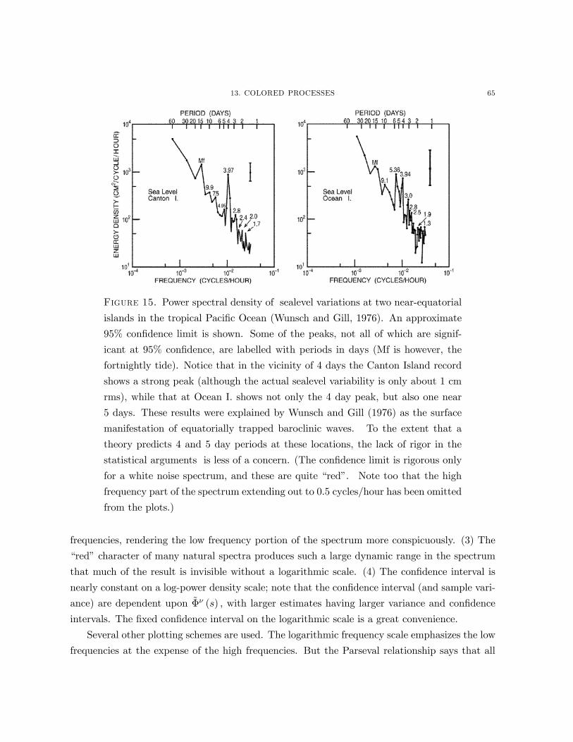
13. COLORED PROCESSES 65
Figure 15. Power spectral density of sealevel variations at two near-equatorial
islands in the tropical Pacific Ocean (Wunsch and Gill, 1976). An approximate
95% confidence limit is shown. Some of the peaks, not all of which are signif-
icant at 95% confidence, are labelled with periods in days (Mf is however, the
fortnightly tide). Notice that in the vicinity of 4 days the Canton Island record
shows a strong peak (although the actual sealevel variability is only about 1 cm
rms), while that at Ocean I. shows not only the 4 day peak, but also one near
5 days. These results were explained by Wunsch and Gill (1976) as the surface
manifestation of equatorially trapped baroclinic waves. To the extent that a
theory predicts 4 and 5 day periods at these locations, the lack of rigor in the
statistical arguments is less of a concern. (The confidence limit is rigorous only
for a white noise spectrum, and these are quite “red”. Note too that the high
frequency part of the spectrum extending out to 0.5 cycles/hour has been omitted
from the plots.)
frequencies, rendering the low frequency portion of the spectrum more conspicuously. (3) The
“red” character of many natural spectra produces such a large dynamic range in the spectrum
that much of the result is invisible without a logarithmic scale. (4) The confidence interval is
nearly constant on a log-power density scale; note that the confidence interval (and sample vari-
ance) are dependent upon Φν (s) , with larger estimates having larger variance and confidence
intervals. The fixed confidence interval on the logarithmic scale is a great convenience.
Several other plotting schemes are used. The logarithmic frequency scale emphasizes the low
frequencies at the expense of the high frequencies. But the Parseval relationship says that all

66 1. FREQUENCY DOMAIN FORMULATION
Figure 16. Power density spectral estimate for pseudorandom numbers (white
noise) with about 12 degrees-of-freedom plotted in three different ways. Upper
left figure is a log-log plot with a single confidence limit shown, equal to the
average for all frequencies. Upper right is a linear plot showing the upper and
lower confidence limits as a function of frequency, which is necessary on a linear
scale. Lower left is the area-preserving form, showing that most of the energy on
the logarithmic frequency scale lies at the high end, but giving the illusion of a
peak at the very highest frequency.
frequencies are on an equal footing, and one’s eye is not good at compensating for the crowding
of the high frequencies. To give a better pictorial representation of the energy distribution, many
investigator’s prefer to plot sΦν (s) on a linear scale, against the logarithm of s. This is sometimes
known as an “area-preserving plot” because it compensates the squeezing of the frequency scale
by the multiplication by s (simultaneously reducing the dynamic range by suppression of the
low frequencies in red spectra). Consider how this behaves (Fig. 16) for white noise. The log-log
plot is flat within the confidence limit, but it may not be immediately obvious that most of the
energy is at the highest frequencies. The area-preserving plot looks “blue” (although we know
this is a white noise spectrum). The area under the curve is proportional to the fraction of
the variance in any fixed logarithmic frequency interval, demonstrating that most of the record
energy is in the high frequencies. One needs to be careful to recall that the underlying spectrum

13. COLORED PROCESSES 67
−6 −5 −4 −3 −2 −1 0
x 106
2
2.5
3
3.5
4
4.5
5
5.5Tiedemann ODB659, δ18O, raw 09−Jun−2000 16:47:43 CW
δ18O
YEARS BP
Figure 17. Time series from a deep-sea core (Tiedemann, et al., 1994). The
time scale was tuned under the assumption that the Milankovitch frequencies
should be prominent.
is constant. The confidence interval would differ in an obvious way at each frequency. A similar
set of plots is shown in Fig. (14) for a real record.
Beginners often use linear-linear plots, as it seems more natural. This form of plot is perfectly
acceptable over limited frequency ranges; it becomes extremely problematic when used over the
complete frequency range of a real record, and its use has clearly distorted much of climate
science. Consider Fig. 17 taken from a tuned ocean core record (Tiedemann, et al., 1994) and
whose spectral density estimate (Fig. 19) is plotted on linear-linear scale.
One has the impression that the record is dominated by the energy in the Milankovitch peaks
(as marked; the reader is cautioned that this core was “tuned” to produce these peaks and a
discussion of their reality or otherwise is beyond our present scope). But in fact they contain
only a small fraction of the record variance, which is largely invisible solely because of the way
the plot suppresses the lower values of the much larger number of continuum estimates. Again
too, the confidence interval is different for every point on the plot.
As one more example, Fig. 20 shows a power density spectrum from altimetric data in
the Mascarene Basin of the western Indian Ocean. This and equivalent spectra were used to
confirm the existence of a spectral peak near 60 days in the Mascarene Basin, and which is
absent elsewhere in the Indian Ocean.
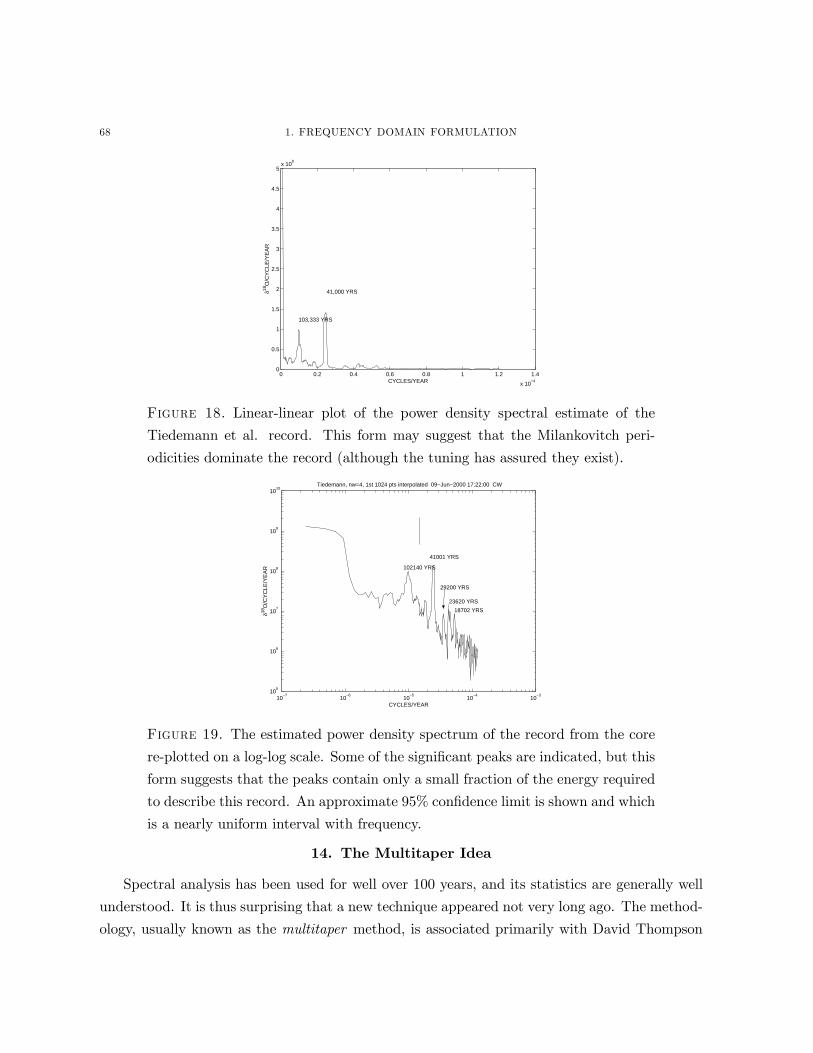
68 1. FREQUENCY DOMAIN FORMULATION
0 0.2 0.4 0.6 0.8 1 1.2 1.4
x 10−4
0
0.5
1
1.5
2
2.5
3
3.5
4
4.5
5x 10
8
CYCLES/YEAR
δ18O
/CY
CLE
/YE
AR
103,333 YRS
41,000 YRS
Figure 18. Linear-linear plot of the power density spectral estimate of the
Tiedemann et al. record. This form may suggest that the Milankovitch peri-
odicities dominate the record (although the tuning has assured they exist).
10−7
10−6
10−5
10−4
10−3
105
106
107
108
109
1010
CYCLES/YEAR
δ18O
/CY
CLE
/YE
AR
Tiedemann, nw=4, 1st 1024 pts interpolated 09−Jun−2000 17:22:00 CW
102140 YRS
41001 YRS
23620 YRS
18702 YRS
29200 YRS
Figure 19. The estimated power density spectrum of the record from the core
re-plotted on a log-log scale. Some of the significant peaks are indicated, but this
form suggests that the peaks contain only a small fraction of the energy required
to describe this record. An approximate 95% confidence limit is shown and which
is a nearly uniform interval with frequency.
14. The Multitaper Idea
Spectral analysis has been used for well over 100 years, and its statistics are generally well
understood. It is thus surprising that a new technique appeared not very long ago. The method-
ology, usually known as the multitaper method, is associated primarily with David Thompson

14. THE MULTITAPER IDEA 69
10−4
10−3
10−2
10−1
105
106
107
108
109
CYCLES/DAY
CM2 /CY
CLE/D
AY
multitaper estimate of power density spectrum 07−Jun−2000
Figure 20. Power density spectra from altimetric data in the western Mascarene
Basin of the Indian Ocean. The result shows (B. Warren, personal communica-
tion, 2000) that an observed 60 day peak (arrow) in current meter records also
appears conspicuously in the altimetric data from the same region. These same
data show no such peak further east. As described earlier, there is a residual alias
from the M2 tidal component at almost exactly the observed period. Identifying
the peak as beng a resonant mode, rather than a tidal line, relies on the narrow
band (pure sinusoidal) nature of a tide, in contrast to the broadband character
of what is actually observed. (Some part of the energy seen in the peak, may
however be a tidal residual.)
of Bell Labs, and is discussed in detail by Percival and Walden (1993). It is probably the best
default methodology. There are many details, but the basic idea is not hard to understand.
Thompson’s approach can be thought of as a reaction to the normal tapering done to a time
series before Fourier transforming. As we have seen, one often begins by tapering xm before
Fourier transforming it so as to suppress the leakage from one part of the spectrum to another.
As Thompson has noted however, this method is equivalent to discarding the data far from
the center of the time series (setting it to small values or zero), and any statistical estimation
procedure which literally throws away data is unlikely to be a very sensible one–real information
is being discarded. Suppose instead we construct a series of tapers, call them w(i)m , 1 ≤ i ≤ P in
such as way thatN−1Xm=0
w(i)m w(j)m = δij (14.1)

70 1. FREQUENCY DOMAIN FORMULATION
that is, they are orthogonal tapers. The first one w(1)m may well look much like an ordinary taper
going to zero at the ends. Suppose we generate P new time series
y(i)m = xmw(i)m (14.2)
Because of the orthogonality of the w(i)m , there will be a tendency for
N−1Xm=0
y(i)m y(j)m ≈ 0, (14.3)
that is, to be uncorrelated. The periodograms¯α(i)k
¯2will thus also tend to be nearly uncorre-
lated and if the underlying process is near-Gaussian, will therefore be nearly independent. We
therefore estimate
Φ2P (s) =1
P
PXi
¯α(i)k
¯2(14.4)
from these nearly independent periodograms.
Thompson showed that there was an optimal choice of the tapers w(i)m and that it is the set
of prolate spheroidal wavefunctions (Fig. 21). For the demonstration that this is the best choice,
and for a discussion of how to compute them, see Percival and Walden (1993) and the references
there to Thompson’s papers. (Note that the prolate spheroidal wave functions are numerically
tricky to calculate, and approximating sinusoids do nearly as well; see McCoy et al., 1998, who
also discuss a special problem with the estimates near zero frequency)
15. Spectral Peaks
Pure sinusoids are very rare in nature, generally being associated with periodic astronomical
phenomena such as tides, or the Milankovitch forcing in solar insolation. Thus apart from
phenomena associated with these forcings, deterministic sinusoids are primarily of mathematical
interest. To the extent that one suspects a pure “tone” in a record not associated with an
astronomical forcing, it would be a most unusual, not-to-say startling, discovery. (These are
called “line spectra”.) If you encounter a paper claiming to see pure frequency lines at anything
other than at the period of an astronomical phenomenon, it’s a good bet that the author doesn’t
know what he is doing. (Many people like to believe that the world is periodic; mostly it isn’t.)
But because both tides and Milankovitch responses are the subject of intense interest in
many fields, it is worth a few comments about line spectra. We have already seen that unlike
a stochastic process, the Fourier coefficients of a pure sinusoid do not diminish as the record
length, N, increases (alternatively, the Fourier transform value increases with N, while for the

15. SPECTRAL PEAKS 71
0 5 10 15 20 25 30 35−0.4
−0.3
−0.2
−0.1
0
0.1
0.2
0.3
0.4
Figure 21. First 4 discretized prolate spheroidal wave functions (also known
as Slepian sequences) used in the multitaper method for a data duration of 32.
Methods for computing these functions are described in detail by Percival and
Walden (1993) and they were found here using a MATLAB toolbox function.
Notice that as the order increases, greater weight is given to data near the ends
of the observations.
stochastic process they remain fixed in rms amplitude). This behavior produces a simple test
of the presence of a pure sinusoid: double (or halve) the record length, and determine whether
the Fourier coefficient remains the same or changes.
Much more common in nature are narrow-band peaks, which represent a relative excess
of energy, but which is stochastic, and not a deterministic sinusoid. A prominent example is
the peak in the current meter spectra (Fig.14) associated with the Coriolis frequency). The
ENSO peak in the Southern Oscillation Index (Wunsch, 1999) is another example, and many
others exist. None of these phenomena are represented by line spectra. Rather they are what
is sometimes called “narrow-band” random processes. It proves convenient to have a common
measure of the sharpness of a peak, and this measure is provided by what electrical engineers call
Q (for “quality factor” associated with a degree of resonance). A damped mass-spring oscillator,
forced by white noise, and satisfying an equation like
md2x
dt2+ r
dx
dt+ kx = θ (t) (15.1)
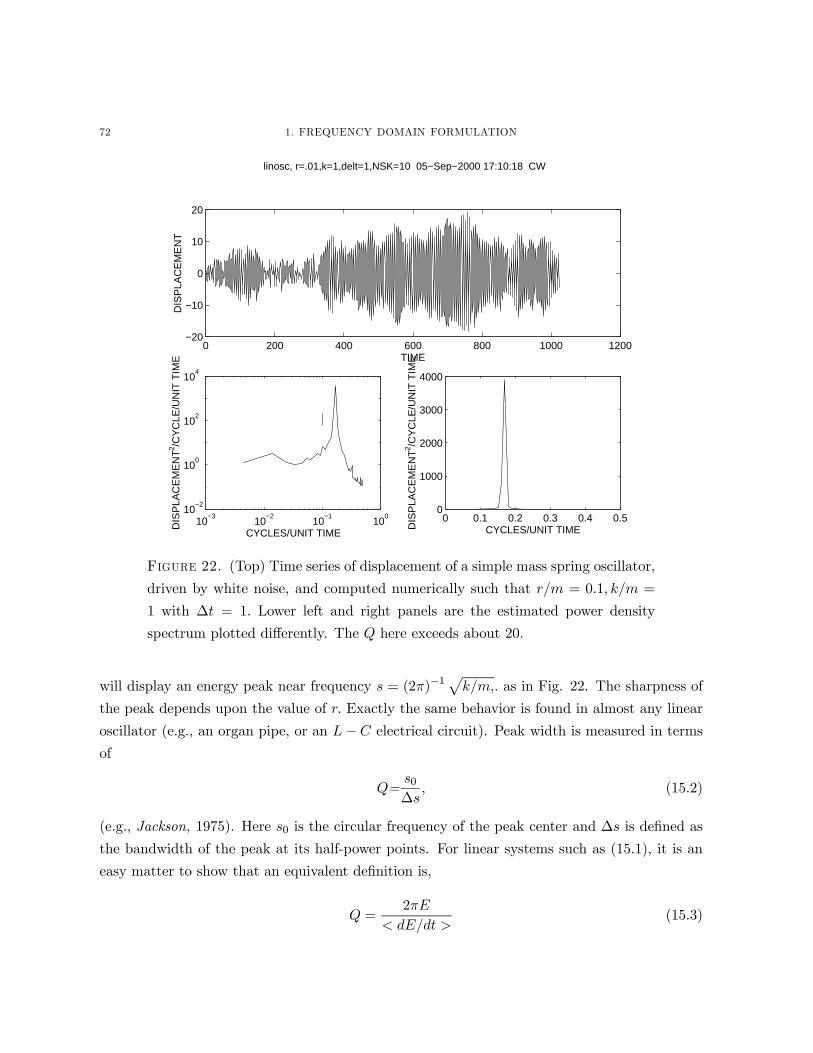
72 1. FREQUENCY DOMAIN FORMULATION
0 200 400 600 800 1000 1200−20
−10
0
10
20
TIME
DIS
PLA
CE
ME
NT
0 0.1 0.2 0.3 0.4 0.50
1000
2000
3000
4000
CYCLES/UNIT TIMEDIS
PLA
CE
ME
NT2 /C
YC
LE/U
NIT
TIM
E
10−3
10−2
10−1
100
10−2
100
102
104
linosc, r=.01,k=1,delt=1,NSK=10 05−Sep−2000 17:10:18 CW
CYCLES/UNIT TIME
DIS
PLA
CE
ME
NT2 /C
YC
LE/U
NIT
TIM
E
Figure 22. (Top) Time series of displacement of a simple mass spring oscillator,
driven by white noise, and computed numerically such that r/m = 0.1, k/m =
1 with ∆t = 1. Lower left and right panels are the estimated power density
spectrum plotted differently. The Q here exceeds about 20.
will display an energy peak near frequency s = (2π)−1pk/m,. as in Fig. 22. The sharpness of
the peak depends upon the value of r. Exactly the same behavior is found in almost any linear
oscillator (e.g., an organ pipe, or an L− C electrical circuit). Peak width is measured in terms
of
Q=s0∆s
, (15.2)
(e.g., Jackson, 1975). Here s0 is the circular frequency of the peak center and ∆s is defined as
the bandwidth of the peak at its half-power points. For linear systems such as (15.1), it is an
easy matter to show that an equivalent definition is,
Q =2πE
< dE/dt >(15.3)

16. SPECTROGRAMS 73
where here E is the peak energy stored in the system, and < dE/dt > is the mean rate of energy
dissipated over one cycle. It follows that for (15.1),
Q =2πs0r
(15.4)
(Jackson, 1975; Munk and Macdonald, 1960, p. 22). As r diminishes, the resonance is greater
and greater, ∆s→ 0, < dE/dt >→ 0, and Q→∞, the resonance becoming perfect.
Exercise. Write (15.1) in discrete form; calculate numerical xm for white noise forcing, and
show that the power density spectrum of the result is consistent with the three definitions of Q.
Exercise. For the parameters given in the caption of Fig. 22, calculate the value of Q.
Values of Q for the ocean tend to be in the range of 1 − 20 (see, e.g., Luther, 1982). Thelowest free elastic oscillation of the earth (first radial mode) has a Q approaching 10,000 (the
earth rings like a bell for months after a large earthquake), but this response is extremely unusual
in nature and such a mode may well be thought of as an astronomical one.
A Practical Point
The various normalizations employed for power densities and related estimates can be con-
fusing if one, for example, wishes to compute the rms amplitude of the motion in some fre-
quency range, e.g., that corresponding to a local peak. Much of the confusion can be evaded
by employing the Parseval relationship (2.4). First compute the record variance, σ2, and form
the accumulating sum Φd (sn) =Pn
k=1
¡a2k + b2k
¢, n ≤ [N/2] , assuming negligible energy in
the mean. Then the fraction of the power lying between any two frequencies, n, n0, must be³Φd (sn)− Φd (s0n)
´/Φd
¡s[N/2]
¢; the root-mean-square amplitude corresponding to that energy
is Ãr³Φd (sn)− Φd (s0n)
´/Φd
¡s[N/2]
¢!σ/√2, (15.5)
and the normalizations used for Φ drop out.
16. Spectrograms
If one has a long enough record, it is possible to Fourier analyze it in pieces, often overlapping,
so as to generate a spectrum which varies with time. Such a record, usually displayed as a contour
plot of frequency and time is known as a “spectrogram”. Such analyses are used to test the
hypothesis that the frequency content of a record is varying with time, implying a failure of the
stationarity hypothesis. The inference of a failure of stationarity has to be made very carefully:
the χ2ν probability density of any spectral estimate implies that there is expected variability
of the spectral estimates made at different times, even if the underlying time series is strictly

74 1. FREQUENCY DOMAIN FORMULATION
stationary. Failure to appreciate this elementary fact often leads to unfortunate inferences (see
Hurrell, 1995 and the comments in Wunsch, 1999).
The need to localize frequency structure in a time-or space-evolving record is addressed
most generally by wavelet analysis. This comparatively recent development is described and
discussed at length by Percival and Walden (2000) but often conventional spectrogram analysis
is completely adequate (if seemingly less sophisticated).
17. Effects of Timing Errors
The problem of errors in the sampling times tm, whether regularly spaced or not, is not a
part of the conventional textbook discussion, because measurements are typically obtained from
instruments for which clock errors are normally quite small. But for instruments whose clocks
drift, but especially when analyzing data from ice or deep ocean cores, the inability to accurately
date the samples is a major problem. A general treatment of clock error or “timing jitter” may
be found in Moore and Thomson (1991) and Thomson and Robinson (1996), with a simplified
version applied to ice core records in Wunsch (2000).
18. Cross-Spectra and Coherence
Definitions
“Coherence” is a measure of the degree of relationship, as a function of frequency, between
two time series, xm, ym. The concept can be motivated in a number of ways. One quite general
form is to postulate a convolution relationship,
ym =∞X−∞
akxm−k + nm (18.1)
where the residual, or noise, nm, is uncorrelated with xm, < nmxp >= 0. The ak are not random
(they are “deterministic”). The infinite limits are again simply convenient. Taking the Fourier
or z−transform of (18.1), we have
y = ax+ n. (18.2)
Multiply both sides of this last equation by x∗ and take the expected values
< yx∗ >= a < xx∗ > + < nx∗ > (18.3)
where < nx∗ >= 0 by the assumption of no correlation between them. Thus,
Φyx (s) = a (s)Φxx (s) , (18.4)
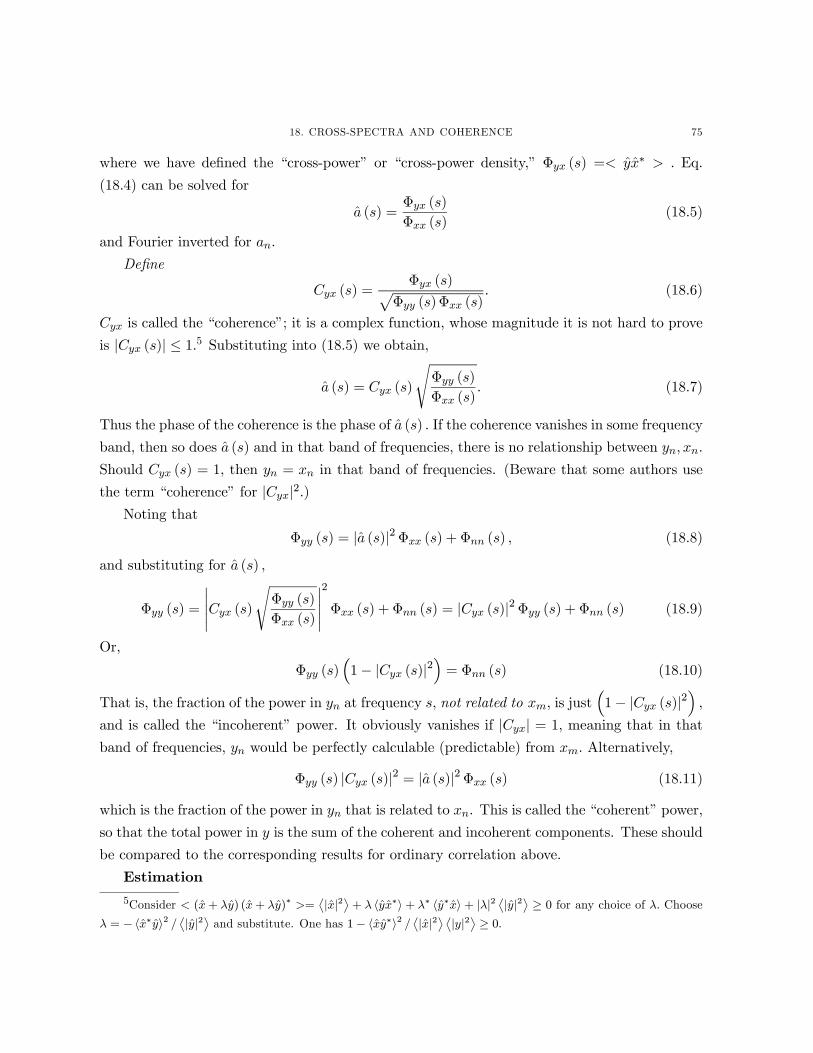
18. CROSS-SPECTRA AND COHERENCE 75
where we have defined the “cross-power” or “cross-power density,” Φyx (s) =< yx∗ > . Eq.
(18.4) can be solved for
a (s) =Φyx (s)
Φxx (s)(18.5)
and Fourier inverted for an.
Define
Cyx (s) =Φyx (s)p
Φyy (s)Φxx (s). (18.6)
Cyx is called the “coherence”; it is a complex function, whose magnitude it is not hard to prove
is |Cyx (s)| ≤ 1.5 Substituting into (18.5) we obtain,
a (s) = Cyx (s)
sΦyy (s)
Φxx (s). (18.7)
Thus the phase of the coherence is the phase of a (s) . If the coherence vanishes in some frequency
band, then so does a (s) and in that band of frequencies, there is no relationship between yn, xn.
Should Cyx (s) = 1, then yn = xn in that band of frequencies. (Beware that some authors use
the term “coherence” for |Cyx|2.)Noting that
Φyy (s) = |a (s)|2Φxx (s) + Φnn (s) , (18.8)
and substituting for a (s) ,
Φyy (s) =
¯¯Cyx (s)
sΦyy (s)
Φxx (s)
¯¯2
Φxx (s) + Φnn (s) = |Cyx (s)|2Φyy (s) + Φnn (s) (18.9)
Or,
Φyy (s)³1− |Cyx (s)|2
´= Φnn (s) (18.10)
That is, the fraction of the power in yn at frequency s, not related to xm, is just³1− |Cyx (s)|2
´,
and is called the “incoherent” power. It obviously vanishes if |Cyx| = 1, meaning that in thatband of frequencies, yn would be perfectly calculable (predictable) from xm. Alternatively,
Φyy (s) |Cyx (s)|2 = |a (s)|2Φxx (s) (18.11)
which is the fraction of the power in yn that is related to xn. This is called the “coherent” power,
so that the total power in y is the sum of the coherent and incoherent components. These should
be compared to the corresponding results for ordinary correlation above.
Estimation
5Consider < (x+ λy) (x+ λy)∗ >= |x|2 + λ hyx∗i+ λ∗ hy∗xi+ |λ|2 |y|2 ≥ 0 for any choice of λ. Chooseλ = − hx∗yi2 / |y|2 and substitute. One has 1− hxy∗i2 / |x|2 |y|2 ≥ 0.

76 1. FREQUENCY DOMAIN FORMULATION
As with the power densities, the coherence has to be estimated from the data. The pro-
cedure is essentially the same as estimating e.g., Φxx (s) . One has observations xn, yn. The
Φxx (s) , Φyy (s) are estimated from the products x (sn) x (sn)∗, etc. as above. The cross-power
is estimated from products y (sn) x (sn)∗ ; these are then averaged for statistical stability in the
frequency domain (frequency band-averaging) or by prior multiplication of each by one of the
multitapers, etc., and the sample coherence obtained from the ratio
Cνyx (s) =
Φνyx (s)qΦνyy (s) Φ
νxx (s)
. (18.12)
Exercise. Let yn = xn + (1/2)xn−1 + θn, where θn is unit variance white noise. Find,
analytically, the coherence, the coherent and incoherent power as a function of frequency and
plot them.
The Blackman-Tukey method would estimate Φνyx (s) via the Fourier transform of the trun-
cated (windowed) sample cross-covariance:
Φνyx (s) = FÃwτ1
N
N−1Xn=0
xnyn+τ
!,
in a complete analogy with the computation by this method of Φνxx (s) , etc. Again, the method
should be regarded as primarily of historical importance, rather than something to be used
routinely today.
Cνyx (s) is a somewhat complicated ratio of complex random variates and it is a problem to
estimate its probability density. As it is a complex quantity, and as the magnitude,¯C (s)
¯, and
phase, φ (s) , have different physical characteristics, the probability densities are sought for both.
The probability density for the amplitude of the sample coherence was studied and tabulated by
Amos and Koopmans (1962). As this reference is not so easily obtained, a summary of the results
are stated here. One has to consider two time series for which the true coherence magnitude, at
frequency s is denoted γ. Then note first, the estimate (18.12) is biassed. For example, if γ = 0
(no coherence), the expected value¯DCνyx (s)
E¯> 0. That is, the sample coherence for two truly
incoherent time series is expected to be greater than zero with a value dependent upon ν. As
ν →∞, the bias goes to zero. More generally, if the coherence is finite,¯< Cν
yx (s) >¯> γ, there
is a tendency for the sample coherence to be too large.
The reasons for the bias are easy to understand. Let us suppose that the cross-power and
auto-power densities are being estimated by a local frequency band averaging method. Then
consider the calculation of Φνyx (s) , as depicted in Fig. 23 under the assumption that γ = 0.

18. CROSS-SPECTRA AND COHERENCE 77
−2 −1.5 −1 −0.5 0 0.5 1 1.5 2−2.5
−2
−1.5
−1
−0.5
0
0.5
1
1.5
2
2.5
Figure 23. The coherence calculation involves summing vectors to produce a
dominant direction (determined by the coherence phase) and amplitude deter-
mined by the degree of coherence. Here the true coherence γ = 0, and ν = 8
random vectors are being summed. That they would sum to a zero-length vector
is very improbable. As ν →∞, the expected length would approach zero.
One is averaging a group of vectors in the complex plane of varying magnitude and direction.
Because the true coherence is zero, the theoretical average should be a zero magnitude vector.
But for any finite number ν of such vectors, the probability that they will sum exactly to zero
is vanishingly small. One expects the average vector to have a finite length, producing a sample
coherence Cνyx (s) whose magnitude is finite and thus biassed. The division by
qΦνyy (s) Φ
νxx (s)
is simply a normalization to produce a maximum possible vector length of 1.
In practice of course, one does not know γ, but must use the estimated value as the best
available estimate. This difficulty has led to some standard procedures to reduce the possibility
of inferential error. First, for any ν, one usually calculates the bias level, which is done by using
the probability density
pC (Z) =2¡1− γ2
¢νΓ (ν)Γ (ν − 1)Z
¡1− Z2
¢ν−2 ∞Xk=0
γ2kΓ2 (ν + k)Z2k
Γ2 (k + 1)(18.13)
for the sample coherence amplitude for γ = 0 and which is shown in Fig. 24 for ν = 8. A
conventional procedure is to determine the value C0 below which¯Cνyx (s)
¯will be confined 95%
of the time. C0 is the “level of no significance” at 95% confidence. What this means is that
for two time series, which are completely uncorrelated, the sample coherence will lie below this
value about 95% of the time, and one would expect, on average for about 5% of the values to
lie (spuriously) above this line. See Fig. 25. Clearly this knowledge is vital to do anything with
a sample coherence.

78 1. FREQUENCY DOMAIN FORMULATION
0 0.1 0.2 0.3 0.4 0.5 0.6 0.7 0.8 0.9 10
0.5
1
1.5
2
2.5
Coherence coefficient
PD
F
PDF of Coherence coeff. for n = 8 γ = 0
Figure 24. Probability density for the sample coherence magnitude, |Cyx (s)| ,when the true value, γ = 0 for ν = 8. The probability of actually obtaining a
magnitude of zero is very small, and the expected mean value is evidently near
0.3.
If a coherence value lies clearly above the level of no significance, one then wishes to place an
error bound on it. This problem was examined by Groves and Hannan (1968; see also Hannan,
1970). As expected, the size of the confidence interval shrinks as γ → 1 (see Fig. 26).
The probability density for the sample coherence phase depends upon γ as well. If γ = 0,
the phase of the sample coherence is meaningless, and the residual vector in Fig. 23 can point
in any direction at all–a random variable of range ±π. If γ = 1, then all of the sample vectorspoint in identical directions, the calculated phase is then exactly found, and the uncertainty
vanishes. In between these two limits, the uncertainty of the phase depends upon γ, diminishing
as γ → 1. Hannan (1970) gives an expression for the confidence limits for phase in the form (his
p. 257, Eq. 2.11): ¯sinhφ (s)− φ (s)
i¯≤∙
1− γ2
(2ν − 2) γ2¸t2ν−2 (α) . (18.14)
Here t2ν−2 (α) is the α% point of Student’s t−distribution with 2ν − 2 degrees of freedom. Analternative approximate possibility is described by Jenkins and Watts (1968, p. 380-381).
Exercise. Generate two white noise processes so that γ = 0.5 at all frequencies. Calculate
the coherence amplitude and phase, and plot their histograms. Compare these results to the
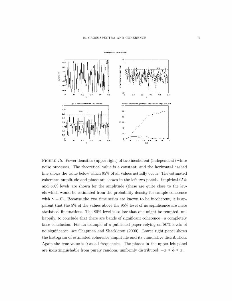
18. CROSS-SPECTRA AND COHERENCE 79
Figure 25. Power densities (upper right) of two incoherent (independent) white
noise processes. The theoretical value is a constant, and the horizontal dashed
line shows the value below which 95% of all values actually occur. The estimated
coherence amplitude and phase are shown in the left two panels. Empirical 95%
and 80% levels are shown for the amplitude (these are quite close to the lev-
els which would be estimated from the probability density for sample coherence
with γ = 0). Because the two time series are known to be incoherent, it is ap-
parent that the 5% of the values above the 95% level of no significance are mere
statistical fluctuations. The 80% level is so low that one might be tempted, un-
happily, to conclude that there are bands of significant coherence–a completely
false conclusion. For an example of a published paper relying on 80% levels of
no significance, see Chapman and Shackleton (2000). Lower right panel shows
the histogram of estimated coherence amplitude and its cumulative distribution.
Again the true value is 0 at all frequencies. The phases in the upper left panel
are indistinguishable from purely random, uniformly distributed, −π ≤ φ ≤ π.

80 1. FREQUENCY DOMAIN FORMULATION
Figure 26. (from Groves and Hannan, 1968). Lower panel displays the power
density spectral estimates from tide gauges at Kwajalein and Eniwetok Islands in
the tropical Pacific Ocean. Note linear frequency scale. Upper two panels show
the coherence amplitude and phase relationship between the two records. A
95% level-of-no-significance is shown for amplitude, and 95% confidence intervals
are displayed for both amplitude and phase. Note in particular that the phase
confidence limits are small where the coherence magnitude is large. Also note
that the confidence interval for the amplitude can rise above the level-of-no-
significance even when the estimated value is itself below the level.
expected probability densities for the amplitude and phase of the coherence when γ = 0. (You
may wish to first read the section below on Simulation.)
Figure 27 shows the coherence between the sealevel record whose power density spectrum
was depicted in Fig. 15 (left) and atmospheric pressure and wind components. Wunsch and Gill
(1976) use the resulting coherence amplitudes and phases to support the theory of equatorially
trapped waves driven by atmospheric winds.

18. CROSS-SPECTRA AND COHERENCE 81
Figure 27. Coherence between sealevel fluctuations and atmospheric pressure,
north wind and eastwind at Canton Island. An approximate 95% level of no
significance for coherence magnitude is indicated. At 95% confidence, one would
expect approximately 5% of the values to lie above the line, purely through
statistical fluctuation. The high coherence at 4 days in the north component of
the wind is employed by Wunsch and Gill (1976, from whom this figure is taken)
in a discussion of the physics of the 4 day spectral peak.
The assumption of a convolution relationship between time series is unnecessary when em-
ploying coherence. One can use it as a general measure of phase stability between two time
series. Consider for example, a two-dimensional wavefield in spatial coordinates r =(rx, ry) and
represented by
η (r,t) =Xn
Xm
anm cos (knm·r− σnmt− φnm) (18.15)
where the anm are random variables, uncorrelated with each other. Define y (t) = η (r1, t) ,
x (t) = η (r2, t) . Then it is readily confirmed that the coherence between x, y is a function of
∆r = r1−r2, as well as σ and the number of wavenumbers knm present at each frequnecy. The

82 1. FREQUENCY DOMAIN FORMULATION
coherence is 1 when ∆r = 0, and with falling magnitude with growth in |∆r| . The way in whichthe coherence declines with growing separation can be used to deduce the number and values of
the wavenumbers present. Such estimated values are part of the basis for the deduction of the
Garrett and Munk (1972) internal wave spectrum.
19. Simulation
In an age of fast computers, and as a powerful test of one’s understanding, it is both useful
and interesting to be able to generate example time series with known statistical properties.
Such simulations can be done both in the frequency and time domains (next Chapter). Suppose
we have a power spectral density, Φ (s)–either a theoretical or an estimated one, and we would
like to generate a time series having that spectral density.
Consider first a simpler problem. We wish to generate a time series of length N, having a
given mean, m, and variance σ2. There is a trap here. We could generate a time series having
exactly this sample mean, and exactly this sample variance. But if our goal is to generate a
time series which would be typical of an actual physical realization of a real process having
this mean and variance, we must ask whether it is likely any such realization would have these
precise sample values. A true coin will have a true (theoretical) mean of 0 (assigning heads as
+1, and tails as -1). If we flip a true coin 10 times, the probability that there will be exactly
5 heads and 5 tails is finite. If we flip it 1000 times, the probability of 500 heads and tails is
very small, and the probability of “break-even” (being at zero) diminishes with growing data
length. A real simulation would have a sample mean which differs from the true mean according
to the probability density for sample means for records of that duration. As we have seen above,
sample means for Gaussian processes have a probability density which is normal G¡0, σ2/N
¢.
If we select each element of our time series from a population which is normal G (0, σ) , the
result will have a statistically sensible sample mean and variance. If we generated 1000 such
time series, we would expect the sample means to scatter about the true mean with probability
density, G¡0, σ2/N
¢.
So in generating a time series with a given spectral density, we should not give it a sample
spectral density exactly equal to the one required. Again, if we generated 1000 such time series,
and computed their estimated spectral densities, we could expect that their average spectral
density would be very close to the required one, with a scattering in a χ2ν distribution. How
might one do this? One way is to employ our results for the periodogram. Using
yq =
[T/2]Xn=1
an cos
µ2πnq
T
¶+
[T/2]−1Xn=1
bn sin
µ2πnq
T
¶. (19.1)

19. SIMULATION 83
0 200 400 600 800 1000−100
−50
0
50
100
150SIMULATED TIME SERIES S−2
TIME
x \h
at
10−4
10−2
100
100
102
104
106
108
Theoretical and Estimated (Multitaper) Power Density Spectrum
FREQUENCY
PO
WE
R /U
NIT
FR
EQ
UE
NC
Y
Figure 28. A simulated time series with power density proportional to s−2.Although just a “red-noise” process, the eye seems to see oscillatory patterns
that are however, ephemeral.
an, bn are generated by a Gaussian-random number generator G (0,Φ (sn)) such that < an >=<
bn >= 0, < a2n >=< b2n >= Φ (s = n/T ) /2, < anam >=< bnbm >= 0,m 6= n, < anbm >= 0.
The requirements on the an, bn assure wide-sense stationarity. Confirmation of stationarity, and
that the appropriate spectral density is reproduced can be simply obtained by considering the
behavior of the autocovariance < ytyq > (see Percival and Walden, 1993). A unit time step,
t = 0, 1, 2, ... is used, and the result is shown in Figure 28.
(This result is rigorously correct only asymptotically as T →∞, or for white noise. The rea-
son is that for finite record lengths of strongly colored processes, the assumption that
hanan0i = hbnbn0i = 0, etc., is correct only in the limit (e.g., Davenport and Root, 1958)).


CHAPTER 2
Time Domain Methods
Time domain methods do not employ any form of transform space to describe a time series
(although it is commonly the case that one can best understand their structures by analyzing
them in the frequency domain). The names most associated with these techniques are Wiener,
and Box and Jenkins. As with the frequency domain methods, one can begin the discussion in
continuous time and it was one of Wiener’s great contributions to show how to deal with that
case. But continuous time representations raise all sorts of complex mathematical issues that
disappear when a time series is made discrete, and so for present purposes, we will begin with
the discrete case of a uniformly sampled time series xt.
1. Representations-1
As with Fourier methods, much of the purpose of these methods is to find efficient represen-
tations of stochastic processes whose interpretation can lead to physical insights. For notational
simplicity, we will assume that ∆t = 1. Consider the simple rule (actually a difference equation
of similar form to (7.1) above),
xm+1 = axm + θm (1.1)
where a is a constant and θm is a zero-mean white noise process of variance σ2θ. Starting with
x0 = 0, (1.1) permits simple generation of realizations of xm depending upon the particular run
of random numbers θm (Fig. 28). We can compute the autocovariance of xm :
R (0) =< x2m >=< (axm−1 + θm−1)2 >= a2R (0) + σ2θ (1.2)
where we used < xm−1θm−1 >= 0, and the assumption that the time-series was wide-sense
stationary (< x2m−1 >=< x2m >= R (0)). So,
R (0) =σ2θ
(1− a2). (1.3)
Evidently, there would be a problem if a = 1, and in fact, |a| < 1 proves to be necessary for thetime-series to be stationary. Similarly,
R (1) =< xm+1xm >=< (axm + θm+1)xm >= aR (0) . (1.4)
85

86 2. TIME DOMAIN METHODS
Exercise. Find R (2) , ..., R (m) for xt in (1.1).
If one knew R (0) and R (1), Eqs. (1.3, 1.4) would fully determine a, σ2θ and they in turn
fully determine everything there is to know about it. Before asking how one might determine
R (0) , R (1) , let us ask where an equation such as (1.1) might arise?
Consider a simple differential system
dx (t)
dt= Ax (t) + g (t) (1.5)
where A is constant and θ is any externally imposed forcing. Equations like this are used
to describe, e.g., a local change in a heat content anomaly, x (t) , as the result of conduction
from a reservoir, heat loss by radiation, and external sources g. Forming simple one-sided time
differences, (1.5) becomes
x (m∆t+∆t) = ∆t (A+ 1)x (m∆t) +∆tg (m∆t) (1.6)
or,
xm+1 = ∆t(A+ 1)xm +∆tgm (1.7)
which is of the form (1.1) with a = ∆t (A+ 1) . Two types of problem exist. In one, gm is
known, and one seeks a; in the other type, gm = θm is unknown and believed to be a white noise
process..
In the second type of problem one has observations of xt and the question is what the best
estimates of a, σ2θ are. Let us try least-squares by minimizing,
J =N−1Xm=0
(xm+1 − axm)2 . (1.8)
The argument here would be that (1.1) can be regarded as an equation which forecasts xm+1from xm, and minimizing the unpredictable part, θm, would give the best possible forecast
system. The normal equations for (1.8) are just one equation in one unknown,
aN−1Xm=0
x2m =N−2Xm=0
xm+1xm. (1.9)
Divide both sides of this equation by N,and we see that it can be written as
aR (0) = R (1) , (1.10)
where we recognize
1
N
N−1Xm=0
x2m, (1.11)

1. REPRESENTATIONS-1 87
as an estimate of the true autocovariance R (0) , and similarly for R (1) . Given the resulting
estimate of a, call it a, one can substitute into (1.8) and compute the estimate σ2θ.
A more general form of the representation of a time-series is,
xm+1 = a1xm + a2xm−1 + ...+ aMxm−M+1 + θm+1, (1.12)
which is called an “autoregressive process of order M” or AR(M), so that (1.1) is an AR(1)
process. To determine the coefficients ai we can proceed again by least-squares, to find the
minimum of
J =N−1Xm=0
(xm+1 − a1xm − a2xm−1 − ...− aMxm−M+1)2 (1.13)
and forming the normal equations,
a1R (0) + a2R (1) + a3R (2) + ..+ aM R (M − 1) = R (1)
a1R (1) + a2R (0) + a3R (1) + ..+ aM R (M − 2) = R (2)
... (1.14)
a1R (M − 1) + a1R (M − 2) + a3R (M − 3) .+ .+ aM R (0) = R (M)
where we used R (−k) = R (k) . Equations (1.14) are usually known as the Yule-Walker equa-
tions. Solving them produces an estimate of the vector of unknowns a = [a1, ...aM ]T and the
value of J is the estimate of σ2θ. If (1.14) is written in matrix form
Ra = b (1.15)
one sees that R is a covariance matrix having the special property that all diagonals have the
same values:
R =
⎧⎪⎪⎪⎪⎪⎪⎪⎨⎪⎪⎪⎪⎪⎪⎪⎩
R (0) R (1) R (2) . R(M − 1)R (1) R (0) R (1) . R(M − 2)R (2) R (1) R (0) . R(M − 3). . . . .
R (m− 1) R(m− 2) R(m− 3) . R (0)
⎫⎪⎪⎪⎪⎪⎪⎪⎬⎪⎪⎪⎪⎪⎪⎪⎭(1.16)
A matrix with constant diagonals is called “Toeplitz”, and the special form of (1.15) permits the
system of equations to be solved without a matrix inversion, using an extremely fast recursive
algorithm called the Levinson (or sometimes, Levinson-Derber) algorithm. This possibility is
less important today than it was in the days before fast computers, but if M is extremely large,
or very large numbers of systems have to be solved, the possibility can remain important.

88 2. TIME DOMAIN METHODS
If gm is a known time-series, one can proceed analogously by minimizing via least-squares,
the objective function
J =N−1Xm=0
(xm+1 − axm − gm)2 (1.17)
with respect to a. Higher order generalizations are obvious, and details are left to the reader.
2. Geometric Interpretation
There is a geometric interpretation of the normal equations. Let us define vectors (of nomi-
nally infinite length) as
xr =
"...xr−1, xr−1, xr,
↑xr+1, xr+2,...
#T(2.1)
θr =
"...θr−1, θr−1, θr,
↑θr+1, θr+2,...
#T(2.2)
where the arrow denotes the time origin (these vectors are made up of the elements of the time
series, “slid over” so that element r lies at the time origin). Define the inner (dot) products of
these vectors in the usual way, ignoring any worries about convergence of infinite sums. Let us
attempt to expand vector xr in terms of M− past vectors:xr = a1xr−1 + a2xr−2 + ...+ aM xr−M + εr (2.3)
where εr is the residual of the fit. Best fits are found by making the residuals orthogonal to the
expansion vectors:
xTr−i (xr − a1xr−1 − a2xr−2 − ...− aM xr−M) = 0, 1 ≤ i ≤M (2.4)
which produces, after dividing all equations by N , and taking the limit as N →∞,
a1R (0) + a2R (1) + ...+ aMR (M − 1) = R (1) (2.5)
a1R (1) + a2R (0) + ...+R(M − 2) = R(2) (2.6)
..., (2.7)
that is precisely the Yule-Walker equations, but with the theoretical values of R replacing the
estimated ones. One can build this view up into a complete vector space theory of time series
analysis. By using the actual finite length vectors as approximations to the infinite length ones,
one connects this theoretical construct to the one used in practice. Evidently this form of time
series analysis is equivalent to the study of the expansion of a vector in a set of (generally
non-orthogonal) vectors.

3. REPRESENTATIONS-2 89
3. Representations-2
An alternative canonical representation of a time series is
xm =MXk=0
akθm−k, (3.1)
(M can be infinite), which called a moving average process of orderM (an MA(M)). Here again
θt is zero-mean white noise of variance σ2θ. Notice that only positive indices ak exist, so that
xm involves only the past values of θk. We can determine these ak by the same least-squares
approach of minimizing an error,
J =N−1Xm=0
Ãxm −
MXk=0
akθm−k
!2, (3.2)
and leading to a set of normal equations, again producing a Toeplitz matrix. As with the AR
problem, the real issue is deciding how large M should be.
Exercise. Derive the normal equations for (3.2) and for J =<³xm −
PMk=0 akθm−k
´2> .
Various theorems exist to show that any stationary discrete time series can be represented
with arbitrary accuracy as either an MA or AR form. Given one form, it is easy to generate the
other. Consider for example (3.1). We recognize that xm is being represented as the convolution
of the finite sequence ak with the sequence θm. Taking the Fourier (or z) transform of xmproduces,
x (z) = a (z) θ (z) (3.3)
or,
θ (z) =x (z)
a (z). (3.4)
Assuming that a (z) has a stable, causal, convolution inverse, such that b (z) = 1/a (z) , we can
write, by taking the inverse transform of (3.4)
θm =LX
k=0
bkxm−k (3.5)
Normalizing b0 = 1, by dividing both sides of the last equation, we can recognize that (3.5) is
in exactly the form of (1.12).
Exercise. Convert the moving average process xm = θm − 1/3θm−1 + 1/4θm−2 into an ARprocess. What order is the AR process?

90 2. TIME DOMAIN METHODS
Because of the reciprocal nature of the vectors a,b in the AR and MA forms, it is generally
true that a finite length a generates a formally infinite length b, and vice-versa (although in
practice, one may well be able to truncate the formally infinite representation without signif-
icant loss of accuracy). The question arises as to whether a combined form, usually called an
autoregressive-moving-average process (or ARMA), might produce the most efficient represen-
tation? That is, one might try to represent a given time series as
xm − a1xm−1 − a2xm−2 − ...− aNxm−N = θt + b1θm−1 + ...+ bMθm−M (3.6)
in such a way that the fewest possible coefficients are required. Taking the z transform of both
sides of (3.6), we obtain
x (z) a (z) = θ (z) b (z) (3.7)
(defining a0 = b0 = 1). One can again use least-squares in either time or frequency domains.
The major issues are once again the best choice of M,N and this problem is discussed at length
in the various references.
Exercise. An ARMA is given as
xm − 12xm−1 = θm − 1
8θm−1 (3.8)
Convert it to (a) an AR, and (b) a MA.
If one has the simplest AR,
xm = axm−1 + θm (3.9)
and takes its Fourier or z-transform, we have
x (z) (1− az) = θ (z) (3.10)
and dividing
x (z) =θ (z)
1− az(3.11)
The Taylor Series about the origin is
x (z) = θ (x)¡1 + az + az2 + az3 + ...
¢(3.12)
which converges on |z| = 1 if and only if |a| < 1 and the corresponding MA form is
xm =∞Xk=0
akθm−k (3.13)
3. REPRESENTATIONS-2 91
where the magnitude of the contribution from the remote past of θm diminishes to arbitrarily
small values. If we nonetheless take the limit a→ 1, we have a process
xm =∞Xk=0
θm−k (3.14)
with an apparent infinite memory of past random forcing. Note that the AR equivalent of (3.14)
is simply
xm = xm−1 + θm (3.15)
–a more efficient representation.
This last process is not stationary and is an example of what is sometimes called an ARIMA
(autoregressive integrated moving average).
Exercise: Show that the process (3.14 or 3.15) has a variance which grows with time.
Despite the non-stationarity, (3.15) is a very simple rule to implement. The resulting time
series has a number of very interesting properties, some of which are described by Wunsch (1999)
and Stephenson et al. (2000) including some discussion of their applicability as a descriptor of
climate change.
Exercise. Using a pseudo-random number generator, form a 10,000 point realization of
(3.15). Calculate the mean and variance as a function of sample length N. How do they behave?
What is the true mean and variance? Find the power density spectrum of the realization and
describe it. Compare the results to realizations from (3.9) with a = 0.9999, 0.99, 0.9 and describe
the behaviors of the sample averages and variance with sample length and the changes in the
spectrum.
Exercise. We can generalize the various representations to vector processes. Let
xm = [x1 (m) , x2 (m) , ...xL (m)]T
be a vector time series of dimension L. Then a vector MA form is
xm =KXk=0
Ak θm−k, (3.16)
where the Ak are matrices, and θm are vectors of white noise elements. Find the normal
equations for determining Ak and discuss any novel problems in their solution. Discuss the
question of whether the Ak should be square matrices or not. Define a vector AR form, and
find the normal equations. What might the advantages be of this approach over treating each
of the scalar elements xj (m) on its own?

92 2. TIME DOMAIN METHODS
4. Spectral Estimation from ARMA Forms
Suppose that one has determined the ARMA form (3.6). Then we have
x (z) =θ (z) b (z)
a (z)(4.1)
or setting z = exp (−2πis) ,
< x (exp(−2πis))x (exp(−2πis))∗ >= Φ (s) =
¯b (exp (−2πis))
¯2|a (exp (−2πis))|2σ
2θ. (4.2)
If a, b are short sequences, then the calculation in (4.2) of the power density spectrum of the time
series can be done essentially analytically. In particular, if b = 1, so that one has a pure AR, the
result is called the “all-pole” method, the power density spectrum being completely determined
by the positions of the zeros of a (z) in the complex z plane. Under some circumstances, e.g.,
when the time series is made up of two pure frequencies differing in frequency by ∆s in the
presence of a white noise background, separation of the two lines can be achieved even if the
record length is such that ∆s < 1/T that is, in violation of the Rayleigh criterion. This
possibility and related considerations lead to what is commonly known as maximum entropy
spectral estimation.
Exercise. Let xm = sin (2πs1m)+sin (2πs2m)+θm,m = 0, 1, ...N. Find an AR representation
of xm and use it to calculate the corresponding power density spectrum.
A considerable vogue developed at one time involving use of “exotic” methods of spectral
representation, including, especially the maximum entropy method. Over time, the fashion has
nearly disappeared because the more astute users recognized that maximum entropy etc. meth-
ods are dangerous: they can give seemingly precise and powerful results apparently unavailable
in the Fourier methods. But these results are powerful precisely because they rely upon the
accuracy of the AR or ARMA etc. model. The sensitivity of e.g., (4.2) to the zero positions
in a (z) means that if the pure pole representation is not the correct one, the appearance of
spectral peaks may be spurious. The exotic methods began to fade with the realization that
many apparent peaks in spectra were the result of an incorrect model. Tukey (1984) and others,
have characterized ARMA-based methods as “covert”, meaning that they hide a whole series of
assumptions, and recommend reliance instead on the “overt” or non-parametric Fourier methods
which are robust and hide nothing. This is good advice except for individuals who know exactly
what they are doing. (Percival and Walden discuss these various methods at length.)

5. KARHUNEN-LOÈVE THEOREM AND SINGULAR SPECTRUM ANALYSIS 93
5. Karhunen-Loève Theorem and Singular Spectrum Analysis
The N ×N, R matrix in Eq. (1.16) is square and symmetric. It is an important result of
linear algebra that such matrices have an orthogonal decomposition
R = VΛVT (5.1)
where Λ is a diagonal matrix, diag{λi} of the eigenvalues of R and V is the matrix of eigen-
vectors V = {vi} , such thatRvi=λivi, (5.2)
and they are orthonormal vTi vj = δij . (It follows that V−1 = VT .)
Let us write a time-series as an expansion in the vq in the form
xn = element n of
⎡⎣ NXq=1
αqpλqvq
⎤⎦ (5.3)
or more succinctly, if we regard xn as an N−element vector, x,
x =
⎡⎣ NXq=1
αqpλqvq
⎤⎦ . (5.4)
Here aq are unit variance, uncorrelated random variates, e.g., G (0, 1) . We assert that such a
time-series has covariance matrix R, and therefore must have the corresponding (by the Wiener-
Khinchin Theorem) power density spectrum. Consider
Rij =< xixj >=NXq=1
NXr=1
< αqαr >pλqλrviqvjr
=NXq=1
λqviqvjq (5.5)
by the covariance properties of αq. But this last equation is just
Rij =©VΛVT
ªij
(5.6)
which is what is required.
Exercise, Confirm (5.6).
Thus (5.4) gives us another way of synthesizing a time series from its known covariance.
That the decomposition (5.4) can always be constructed (in continuous time) for a stationary
time series is called the Karhunen-Loève Theorem (see Davenport and Root, 1958). Because
it is based upon a decomposition of the covariance matrix, it is evidently a form of empirical

94 2. TIME DOMAIN METHODS
orthogonal function synthesis, or if one prefers, an expansion in principal components (see e. g.,
Jolliffe, 1986).
The relative importance of any orthogonal structure, vi, to the structure of xn, is controlled
by the magnitude of√λi. Suppose one has been successful in obtaining a physical interpretation
of one or more of the important vi. Each of these vectors is itself a time series. One can evidently
compute a power density spectrum for them, either by Fourier or more exotic methods. The idea
is that the spectra of the dominant vi are meant to be informative about the spectral properties
of processes underlying the full time series. This hypothesis is a plausible one, but will only
be as valid as the reality of the underlying physical structure attributed to vi. (At least two
issues exist, determining when λi is significantly different from zero, and obtaining a physical
interpretation of the components. Principal components are notoriously difficult to relate to
normal modes and other physically generated structures.) This subject has come to be known
as “singular spectrum analysis” (e.g. Vautard and Ghil, 1989) and its powers (and statistical
information such as confidence limits) are still murky.
6. Wiener and Kalman Filters
6.1. The Wiener Filter. The theory of filtering of stationary time series for a variety of
purposes was constructed by Norbert Wiener in the 1940s for continuous time processes in a
notable feat of mathematics (Wiener, 1949). The work was done much earlier, but was classified
until well after World War II). In an important paper however, Levinson (1947) showed that in
discrete time, the entire theory could be reduced to least squares and so was mathematically
very simple. This approach is the one used here. Note that the vector space method sketched
above is fully equivalent too.
The theory of Wiener filters is directed at operators (filters) which are causal. That is, they
operate only upon the past and present of the time series. This requirement is essential if one
is interested in forecasting so that the future is unavailable. (When the future is available, one
has a “smoothing” problem.) The immediate generator of Wiener’s theory was the need during
the Second World War for determining where to aim anti-aircraft guns at dodging airplanes. A
simple (analogue) computer in the gunsight could track the moving airplane, thus generating a
time history of its movements and some rough autocovariances. Where should the gun be aimed
so that the shell arrives at the position of the airplane with smallest error? Clearly this is a
forecasting problem. In the continuous time formulation, the requirement of causality leads to
the need to solve a so-called Wiener-Hopf problem, and which can be mathematically tricky. No
such issue arises in the discrete version, unless one seeks to solve the problem in the frequency
domain where it reduces to the spectral factorization problem alluded to in Chapter 1.

6. WIENER AND KALMAN FILTERS 95
The Wiener Predictor
Consider a time series xm with autocovariance Rxx (τ) (either from theory or from prior
observations). We assume that xm, xm−1, ..., are available; that is, that enough of the past isavailable for practical purposes (formally the infinite past was assumed in the theory, but in
practice, we do not, and cannot use, filters of infinite length). We wish to forecast one time step
into the future, that is, seek a filter to construct
xm+1 = a0xm + a1xm−1 + ..+ aMxm−M =MXk=0
akxm−k, (6.1)
such that the ai are fixed. Notice that the causality of ak permits it only to work on present
(time m) and past values of xp. We now minimize the “prediction error” for all times:
J =Xm
(xm+1 − xm+1)2 . (6.2)
This is the same problem as the one leading to (1.14) with the same solution. The prediction
error is just
P =< (xm+1 − xm+1)2 >
= R(0)− 2MXk=0
akR (k + 1) +MXk=1
MXl=1
akalR(k − l) ≤ R (0) . (6.3)
Notice that if xm is a white noise process, R (τ) = σ2xxδτ0, ai = 0, and the prediction error
is σ2xx. That is to say, the best prediction one can make is xm+1 = 0 and Eq. (6.3) reduces to
P = R (0) , the full variance of the process and there is no prediction skill at all. These ideas
were applied by Wunsch (1999) to the question of whether one could predict the NAO index
with any skill through linear means. The estimated autocovariance of the NAO is shown in
Fig. 1 (as is the corresponding spectral density). The conclusion was that the autocovariance is
so close to that of white noise (the spectrum is nearly flat), that while there was a very slight
degree of prediction skill possible, it was unlikely to be of any real interest. (The NAO is almost
white noise.) Colored processes can be predicted with a skill depending directly upon how much
structure their spectra have.
Serious attempts to forecast the weather by Wiener methods were made during the 1950s.
They ultimately foundered with the recognition that the atmosphere has an almost white noise
spectrum for periods exceeding a few days. The conclusion is not rigidly true, but is close enough
that what linear predictive skill could be available is too small to be of practical use, and most
sensible meteorologists abandoned these methods in favor of numerical weather prediction (which
however, is still limited for related reasons, to skillful forecasts of no more than a few days). It

96 2. TIME DOMAIN METHODS
−150 −100 −50 0 50 100 150−100
0
100
200
300
400
500
600
LAG TIME
AUTOCOVAR., NAO WINTER 04−Sep−2000 20:18:26 CW
Figure 1. The estimated autocovariance of the North Atlantic Oscillation Index
(NAO). Visually, and quantitatively, the autocovariance is dominated by the spike
at the origin, and differs little from the autocovariance of a white noise process.
By the Wiener filter theory, it is nearly unpredictable. See Wunsch (1999).
is possible that spatial structures within the atmosphere, possibly obtainable by wavenumber
filtering, would have a greater linear prediction possibility. This may well be true, but they would
therefore contain only a fraction of the weather variance, and one again confronts the issue of
significance. To the extent that the system is highly non-linear (non-Gaussian), it is possible
that a non-linear filter could do better than a Wiener one. It is possible to show however, that
for a Gaussian process, no non-linear filter can do any better than the Wiener one.
Exercise. Find the prediction error for a forecast at k−time steps into the future.
Exercise. Consider a vector time series, xm = [hm, gm]T , where < hmgm >6= 0. Generalize
the Wiener prediction filter to this case. Can you find a predictive decomposition?
A slightly more general version of the Wiener filter (there are a number of possibilities) is
directed at the extraction of a signal from noise. Let there be a time series
xm = Sm + nm (6.4)
where Sm is the signal which is desired, and nm is a noise field. We suppose that < Smnm >= 0
and that the respective covariances RSS (τ) =< SmSm+τ >, Rmn (τ) =< nmnm+τ > are known,

6. WIENER AND KALMAN FILTERS 97
at least approximately. We seek a filter, am, acting on xm so thatXm
amxk−m ≈ Sk (6.5)
as best possible. (The range of summation has been left indefinite, as one might not always
demand causality.) More formally, minimize
J =N−1Xk=0
ÃSk −
Xm
amxk−m
!2. (6.6)
Exercise. Find the normal equations resulting from (6.6). If one takes Sm = xm+1, is the
result the same as for the prediction filter? Suppose am is symmetric (that is acausal), take the
Fourier transform of the normal equations, and using the Wiener-Khinchin theorem, describe
how the signal extraction filter works in the frequency domain. What can you say if ak is forced
to be causal?
6.2. The Kalman Filter. R. Kalman (1960) in another famous paper, set out to extend
Wiener filters to non-stationary processes. Here again, the immediate need was of a military
nature, to forecast the trajectories of ballistic missiles, which in their launch and re-entry phases
would have a very different character than a stationary process could describe. The formalism
is not very much more complicated than for Wiener theory, but is best left to the references (see
e.g., Wunsch, 1966, Chapter 6). But a sketch of a simplified case may perhaps give some feeling
for it.
Suppose we have a “model” for calculating how xm will behave over time. Let us assume,
for simplicity, that it is just an AR(1) process
xm = axm−1 + θm. (6.7)
Suppose we have an estimate of xm−1, called xm−1, with an estimated error
Pm−1 =< (xm−1 − xm−1)2 > . (6.8)
Then we can make a forecast of xm,
xm (−) = axm−1 (6.9)
because θm is unknown and completely unpredictable by assumption. The minus sign in the
argument indicates that no observation from time m has been used. The prediction error is now
Pm (−) =< (xm (−)− xm)2 >= σ2θ + Pm−1, (6.10)
98 2. TIME DOMAIN METHODS
that is, the initial error propagates forward in time and is additive to the new error from the
unknown θm. Now let us further assume that we have a measurement of xm but one which has
noise in it,
ym = Exm + εm, (6.11)
where < εm >= 0, < ε2m >= σ2ε, which produces an estimate ym/E, with error variance E−2σ2ε.
The observation of xm ought to permit us to improve upon our forecast of it, xm (−) . A plausibleidea is to average the measurement with the forecast, weighting the two inversely as their relative
errors:
xm =σ2θ + Pm−1¡
σ2θ + Pm−1¢+E−2σ2ε
E−1ym +E−2σ2ε¡
σ2θ + Pm−1¢+E−2σ2ε
xm (−) (6.12)
= xm (−) +¡σ2θ + Pm−1
¢E−1¡
σ2θ + Pm−1¢+E−2σ2ε
(ym −Exm (−)) (6.13)
(See Wunsch, 1996, section 3.7). If the new data are very poor relative to the forecast, σ2ε →∞,
the estimate reduces to the forecast. In the opposite limit when¡σ2θ + Pm−1
¢>> E−2σ2ε, the
new data give a much better estimate, and it can be confirmed that xm → ym/E as is also
sensible.
The expected error of the average is
Pm =h¡E−2σ2ε
¢−1+¡σ2θ + Pm−1
¢−1i−1(6.14)
=¡σ2θ + Pm
¢− ¡σ2θ + Pm−12¢2 £¡
σ2θ + Pm−1¢+E−2σ2ε
¤−1, (6.15)
which should be studied in the two above limits. Now we proceed another time-step into the
future. The new best forecast is,
xm+1 = axm (6.16)
where xm has error Pm and we proceed just as before, with m → m + 1. If there are no
observations available at time m, then the forecast cannot be improved, xm+1 = axm, and one
keeps going with xm+2 = axm+1. The Kalman filter permits one to employ whatever information
is contained in a model (perhaps dynamical, as in orbital equations or an ocean circulation model)
along with any observations of the elements of the system that come in through time. The idea
is extremely powerful and many thousands of papers and books have been written on it and its
generalizations.1 If there is a steady data stream, and the model satisfies certain requirements,
one can show that the Kalman filter asymptotically reduces to the Wiener filter–an important
conclusion because the Kalman formalism is generally computationally much more burdensome
1Students may be interested to know that it widely rumored that Kalman twice failed his MIT general exams
(in EECS).

7. GAUSS-MARKOV THEOREM 99
than is the Wiener one. The above derivation contains the essence of the filter, the only changes
required for the more general case being the replacement of the scalar state x (t) by a vector
state, x (t) , and with the covariances becoming matrices whose reciprocals are inverses and one
must keep track of the order of operations.
6.3. Wiener Smoother. “Filtering” in the technical sense involves using the present and
past, perhaps infinitely far back, of a time-series so as to produce a best estimate of the value of
a signal or to predict the time series. In this situation, the future values of xm are unavailable.
In most oceanographic problems however, we have a stored time series and the formal future is
available. It is unsurprising that one can often make better estimates using future values than
if they are unavailable (just as interpolation is more accurate than extrapolation). When the
filtering problem is recast so as to employ both past and future values, one is doing “smoothing”.
Formally, in equations such as (6.5, 6.6), one permits the index m to take on negative values
and finds the new normal equations.
7. Gauss-Markov Theorem
It is often the case that one seeks a signal in a noise background. Examples would be the
determination of a sinusoid in the presence of a background continuum stochastic process, and
the determination of a trend in the presence of other processes with a different structure. A
perhaps less obvious example, because it is too familiar, is the estimation of the mean value of
a time series, in which the mean is the signal and the deviations from the mean are therefore
arbitrarily defined as the “noise.” The cases one usually encounters in elementary textbooks and
classes are some simple variant of a signal in presence of white noise. Unfortunately, while this
case is easy to analyze, it usually does not describe the situation one is faced with in practice,
when for example, one must try to determine a trend in the presence of red noise processes, ones
which may exhibit local trends easily confused with a true secular (deterministic) trend. This
problem plagues climate studies.
There are several approaches to finding some machinery which can help one to fall into
statistical traps of confusing signal with noise. One widely applicable methodology is called
variously “minimum variance estimation”, the “Gauss-Markov Theorem”, and in a different
context, sometimes the “stochastic inverse.” Although a more extended discussion is given in
Wunsch (1996), or see Liebelt (1967) for a complete derivation, the following heuristic outline
may help.
Let there be some set of N unknown parameters, written here as a vector, s. We suppose
that they have zero mean, < s >= 0, and that there is a known covariance for s, Rss =ssT
®.

100 2. TIME DOMAIN METHODS
Let there be a set of M measurements, written here also as another vector y, also with zero
mean, and known covariance < yyT >= Ryy. Finally, we will assume that there is a known
covariance between the measurements and the unknowns: Rsy =< syT > . Given these covari-
ances (correlations), what can we say about s, given y, if we try to estimate any of the elements
si, as a linear combination of the measurements:
si =MXj=1
Bijyj . (7.1)
The question is, how should the weights, Bij be chosen? Arbitrarily, but reasonably, we seek
Bij such that the variance of the estimated si about the true value is as small as possible, that
is, D(si − si)
2E=
*⎛⎝ mXj=1
Bijyj − si
⎞⎠2+, 1 ≤ i ≤ N (7.2)
should be a minimum. Before proceeding, note that Bij is really a matrix, and each row will
be separately determinable for each element si. This simple observation permits us to re-write
(7.2) in a matrix-vector form. Minimize the diagonal elements of:
< (s− s) (s− s)T >=< (By − s) (By− s)T >≡ P. (7.3)
The important point here is that, in (7.3), we are meant to minimize the N separate diagonal
elements, each separately determining a row of B; but we can use the notation to solve for all
rows simultaneously.
At this stage, one expands the matrix product in (7.3), and uses the fact that quantities such
as < ssT >= Rss are known. One can show without too much difficulty (it involves invoking
the properties of positive definite matrices) that the minimum of the diagonals is given by the
unique choice,
B = RsyR−1yy , (7.4)
with the first row being the solution for s1, etc.
The result (7.4) is general and abstract. Let us now consider a special case in which the
measurements yq are some linear combination of the parameters, corrupted by noise, that is,
yq =PN
l=1Eqlsl + nq, which can also be written generally as,
Es+ n = y. (7.5)
With this assumption, we can evaluate
Rsy =< s (Es+ n)T >= RssE
T , (7.6)

7. GAUSS-MARKOV THEOREM 101
assuming < snT >= 0, and
Ryy = ERssET +Rnn (7.7)
where Rnn =< nnT >. Then one has immediately,
B = Rss
¡ERssE
T+Rnn
¢−1, (7.8)
and
s = Rss
¡ERssE
T+Rnn
¢−1y. (7.9)
There is one further, extremely important step: how good is this estimate? This question is
readily answered by substituting the value of B back into the expression (7.3) for the actual
covariance about the true value. We obtain immediately,
P = Rss −RssET¡ERssE
T+Rnn
¢ERss. (7.10)
One of the benefits of the general approach is that we have obtain the complete matrix P, which
gives us not only the variances (uncertainties) of each of the si about the true value, but also
the covariances of these errors or uncertainties in each, with all the others–they do after all,
depend upon the same data–so that it is no surprise that they would have correlated errors.)
A special case, written out in Wunsch (1996), and which is particularly illuminating is the
simple problem of determining a mean value (so that s is a scalar), in the presence of a noise field
which has an arbitrary correlation. One finds there, that the uncertainty of the mean can be
vastly greater than the conventional estimates based upon white noise, if the noise is correlated
in time.
Remark 2. A common complaint among beginning users of Gauss-Markov and related es-
timation methods is: “I have no idea what the covariances are. This all becomes completely
arbitrary if I just make up something.” The answer to this worry is found by examining the
statement “I have no idea what the covariances are.” If this is really true, it means that an
acceptable answer for any element, si could have any value at all, including something infin-
itesimal, 10−40, or astronomical, ±1040 and one would say “that’s acceptable, because I knownothing at all about the solution”. The reader may say, “that’s not what I really meant”. In
fact, it is extremely rare to be completely ignorant, and if one is completely ignorant, so that
any values at all would be accepted, the investigator ought perhaps to stop and ask if the problem
makes any sense? More commonly, one usually knows something, e.g., that the parameters are
very unlikely to be bigger than about ±S0. If that is all one is willing to say, then one simplytakes
Rss = S20IN (7.11)

102 2. TIME DOMAIN METHODS
with something analogous perhaps, for Rnn, which becomes an estimate of the noise magnitude.
Letting S20 →∞ is the appropriate limit if one really knows nothing, and one might study 7.10)
in that limit. The point is, that the estimation procedure can use whatever information one has,
and one need not stipulate anything that is truly unknown. In particular, if one does not know
the non-diagonal elements of the covariances, one need not state them. All that will happen is
that a solution will be obtained that likely will have a larger uncertainty than one could have
obtained had additional information been available. The more information one can provide, the
better the estimate. A final comment of course, is that one must check that the solution and the
errors left are actually consistent with what was postulated for the covariances. If the solution
and noise residuals are clearly inconsistent with Rss, etc., one should trash the solution and try
to understand what was wrong; this is a very powerful test, neglected at one’s peril. If used, it
can rescue even the naivest user from a truly silly result.
8. Trend Determination
A common debate in climate and other studies concerns the reality of trends in data. Specif-
ically, one is concerned that an apparent linear or more complex trend should be distinguished,
as secular, from local apparent trends which are nothing but the expected short-term behavior of
a stochastic process. The synthetic time series displayed above show extended periods where one
might be fooled into inferring a trend in climate, when it is nothing but a temporary structure
occurring from pure happenstance. For geophysical problems, the existence of rednoise time
series makes the problem quite difficult.
Suppose one has a stationary time series xq whose power density and corresponding autoco-
variance R (τ) are known. From R (τ) we can make a covariance matrix as in (1.16). We suspect
that superimposed upon this time series is a linear secular trend representable as yq = a+bq and
we would like to determine a, b and their uncertainty. Generalizing the discussion in Wunsch
(1996, p.188), we regard xq now as a noise process and a+bq as a signal model. We can represent
a+ bq + xq = gq, or
Da+ x = g, (8.1)
where,
a = [a, b]T ,D =
⎧⎪⎪⎪⎪⎪⎪⎪⎨⎪⎪⎪⎪⎪⎪⎪⎩
1 0
1 1
1 2
. .
1 N − 1
⎫⎪⎪⎪⎪⎪⎪⎪⎬⎪⎪⎪⎪⎪⎪⎪⎭,g =[g0, g1, ..., gN−1]T . (8.2)

9. EOFS, SVD 103
Suppose that no a priori statistical information about a, b is available (that is, we would accept
arbitrarily large or small values as the solution). Then the Gauss-Markov Theorem produces a
best-estimate
a =
"a
b
#=£DTRD
¤−1DTR−1g (8.3)
with uncertainty
P =< (a− a)2 >= ¡DTR−1D¢−1
. (8.4)
Clearly P depends directly upon the covariance R. If long-temporal correlations are present,
apparent, but spurious trends, will probably be found. But the result (8.3) will have large
expected uncertainties given by (8.4) and one would not be misled.
Exercise. Generate a time series with power density Φ (s) = 1/(5/4 + cos (2πs)). Add a
known trend, and then determine it from the above expressions.
Trend determination is an important special case of time-domain analysis. The methodology
used here is straightforward if the trend is to be determined over the entire record. But what one
cannot do with this method, without modification, is to look at a record by eye, and say “there
seems to be a trend beginning at time t1 and running to the end of the record. I’ll determine
the trend over that interval.” One can certainly determine such a trend; the issue lies with the
error estimate associated with the result. By deciding the time at which the trend begins, one
is greatly reducing the number of degrees-of-freedom. Alternatively, one is imposing posterior
knowledge and the statistics based purely upon a priori knowledge are no longer valid. Percival
and Rothrock (2005) have a good discussion of the issue. (Almost all time series have trends
over some interval. Clearly one should not select such an interval and proclaim the trend to be
statistically significant when it is clear that it terminates. At the end of the record, one does
not necessarily see the termination.)
9. EOFs, SVD
A common statistical tool in oceanography, meteorology and climate research are the so-
called empirical orthogonal functions (EOFs). Anyone, in any scientific field, working with
large amounts of data having covariances, is almost inevitably led to EOFs as an obvious tool
for reducing the number of data one must work with, and to help in obtaining insight into the
meaning of the covariances that are present. The ubiquity of the tool means, unfortunately, that
it has been repeatedly reinvented in different scientific fields, and the inventors were apparently
so pleased with themselves over their cleverness, they made no attempt to see if the method was

104 2. TIME DOMAIN METHODS
already known elsewhere. The consequence has been a proliferation of names for the same thing:
EOFs, principal components, proper orthogonal decomposition, singular vectors, Karhunen-
Loève functions, optimals, etc. (I’m sure this list is incomplete.)
The method, and its numerous extensions, is a useful one (but like all powerful tools, poten-
tially dangerous to the innocent user), and a brief discussion is offered here. The most general
approach of which I am aware, is that based upon the so-called singular value decomposition
(e.g., Wunsch, 1996 and references there). Let us suppose that we have a field which varies, e.g.,
in time and space. An example (often discussed) is the field of seasurface temperature (SST) in
the North Pacific Ocean. We suppose that through some device (ships, satellites), someone has
mapped the anomaly of SST monthly over the entire North Pacific Ocean at 1◦ lateral resolutionfor 100 years. Taking the width of the Pacific Ocean to be 120◦ and the latitude range to be60◦ each map would have approximately 60×120 = 7200 gridded values, and there would be
12×100 of these from 100 years. The total volume of numbers would then be about 7200×1200or about 9 million numbers.
A visual inspection of the maps (something which is always the first step in any data analy-
sis), would show that the fields evolve only very slowly from month-to-month in an annual cycle,
and in some respects, from year-to-year, and that much, but perhaps not all, of the structure
occurs on a spatial scale large compared to the 1◦ gridding. Both these features suggest thatthe volume of numbers is perhaps much greater than really necessary to describe the data, and
that there are elements of the spatial structure which seem to covary, but with different fea-
tures varying on different time scales. A natural question then, is whether there is not a tool
which could simultaneously reduce the volume of data, and inform one about which patterns
dominated the changes in space and time? One might hope to make physical sense of the latter.
Because there is such a vast body of mathematics available for matrices, consider making a
matrix out of this data set. One might argue that each map is already a matrix, with latitude
and longitude comprising the rows and columns, but it suits our purpose better to make a single
matrix out of the entire data set. Let us do this by making one large column of the matrix out
of each map, in some way that is arbitrary, but convenient, e.g., by stacking the values at fixed
longitudes in one long column, one under the other (we could even have a random rule for where
in the column the values go, as long it is the same for each time–this would just make it hard
to figure out what value was where). Then each column is the map at monthly intervals, with
1200 columns. Call this matrix E, which is of dimension M =number of latitudes times the
number of longitudes by N, the number of observation times (that is, it is probably not square).
9. EOFS, SVD 105
We now postulate that any matrix E can be written
E = UΛVT (9.1)
that is as the product of three matrices. Λ is a M ×N diagonal matrix (in a generalized sense
for a non-square matrix). Matrix U is square of dimension M, and V is square of dimension N.
U,V have the special properties of being “orthogonal”,
UUT= IM ,UTU = IM ,VVT= IN ,VTV = IN (9.2)
that is to say, in particular the columns of U are mutually orthonormal, as are the columns of
V (so are the rows, but that proves less important). IN is the identity matrix of dimension N,
etc. The matrices U,V,Λ can be shown, with little difficulty to be determined by the following
relations:
EETui=λ2iui, 1 ≤ i ≤M, ETEvi=λ
2ivi, 1 ≤ i ≤ N. (9.3)
That is to say, the columns of U are the eigenvectors of EET , and the columns of V are the
eigenvectors of ETE. They are related to each other through the relations,
Evi=λiui,1 ≤ i ≤ N, Eui=λivi, 1 ≤ i ≤M. (9.4)
Note that in (9.3,9.4), M,N are in general different, and the only way these relationships
can be consistent would be if all of the λi = 0, i > min (M,N) (this is the maximum number of
non-zero eigenvalues; there may be fewer). By convention, the λi and their corresponding ui,viare ordered in decreasing value of the λi.
Consider ETE in (9.3) This new matrix is formed by taking the dot product of all of the
columns of E with each other in sequence. That is to say, ETE is, up to a normalization
factor of 1/M, the covariance of each anomaly map with every other anomaly map and is thus
a covariance matrix of the observations through time and the vi are the eigenvectors of this
covariance matrix. Alternatively, EET is the dot product of each row of the maps with each
other, and up to a normalization of 1/N is the covariance of the structure at each location in
the map with that at every other point on the map; the ui are thus the eigenvectors of this
covariance matrix.
Consider by way of example, ETE. This is a square, non-negative definite matrix (meaning
its eigenvalues are all non-negative, a good thing, since the eigenvalues are the λ2i , which we
might hope would be a positive number). From (9.1, 9.2),
ETE = VΛ2VT =NXi=1
λ2ivivTi , (9.5)

106 2. TIME DOMAIN METHODS
Eq. (9.5) is an example of the statement that a square, symmetric matrix can be represented
exactly in terms of its eigenvectors. Suppose, only K ≤ N of the λi are non-zero. Then the sum
reduces to,
ETE =KXj=1
λ2ivivTi = VKΛ
2KV
TK , (9.6)
where ΛK is truncated to its first K rows and columns (is now square) and VK contains only
the first k columns of V. Now suppose that some of the λi are very small compared, e.g., to the
others. Let there be K 0 of them, much larger than the others. The question then arises as towhether the further truncated expression,
ETE ∼K0Xi=1
λ2ivivTi = VK0Λ2K0VT
K0 , (9.7)
is not still a good approximation to ETE? Here, VK0 consists only of its first K 0 columns.The assumption/conclusion that the truncated expansion (9.7) is a good representation of the
covariance matrix ETE, with K 0 << K is the basis of the EOF idea. Conceivably K 0 is as smallas 1 or 2, even when there may be hundreds or thousands of vectors vi required for an exact
result. An exactly parallel discussion applies to the covariance matrix EET in terms of the ui.
There are several ways to understand and exploit this type of result. Let us go back to (9.1).
Assuming that there are K non-zero λi, it can be confirmed (by just writing it out) that
E = UKΛKVTK =
KXi=1
λiuivTi (9.8)
exactly. This result says that an arbitrary M ×N matrix E can be represented exactly by at
most K pairs of orthogonal vectors, where K ≤ min (M,N) . Suppose further, that some of the
λi are very small compared to the others Then one might suppose that a good approximation
to E is
E ∼ UKΛK0VTK0 =
K0Xi=1
λiuivTi . (9.9)
If this is a good approximation, and K 0 << K, and because E are the actual data, it is possible
that only a very small number of orthogonal vectors is required to reproduce all of the significant
structure in the data. Furthermore, the covariances of the data are given by simple expressions
such as (9.7) in terms of these same vectors.
The factorizations (9.1) or the alternative (9.8) are known as the “singular value decom-
position”. The λi are the “singular values”, and the pairs (ui,vi) are the singular vectors.
Commonly, the vi are identified as the EOFs, but they can equally well be identified as the ui;
the choice is arbitrary, depending only upon how one seeks to interpret the data.

9. EOFS, SVD 107
Eq. (9.9) can be discussed slightly differently. Suppose that one has an arbitrary E. Then
if one seeks to represent it in L pairs of orthonormal vectors (qi, ri)
E ≈LXi=1
αiqirTi , (9.10)
then the so-called Eckart-Young-Mirsky theorem (see references in Wunsch, 1996) states that
the best choice (in the sense of making the norm of the difference between the left and right-hand
sides as small as possible), is for the(qi, ri) to be the first L singular vectors, and αi = λi.
Exercise. Interpret the Karhunen-Loève expansion and singular spectrum analysis in the
light of the SVD.
Exercise. (a) Consider a travelling wave y (r, t) = sin (kr + σt) , which is observed at a
zonal set of positions, rj = (j − 1)∆r at times tp = (p− 1)∆t. Choose, k, σ,∆r,∆t so that thefrequency and wavenumber are resolved by the time/space sampling. Using approximately 20
observational positions and enough observation times to obtain several temporal periods, apply
the SVD/EOF analysis to the resulting observations. Discuss the singular vectors which emerge.
Confirm that the SVD at rank 2 perfectly reproduces all of the data. The following, e.g., would
do (in MATLAB)
» x=[0:30]’;t=[0:256]’;
» [xx,tt]=meshgrid(x,t);
» sigma=2*pi/16;k=2*pi/10;
» Y=sin(k*xx+sigma*tt);
» contourf(Y);colorbar;
(b) Now suppose two waves are present: y (r, t) = sin (kr + σt) + sin((k/2) r + (σ/2) t).
What are the EOFs now? Can you deduce the presence of the two waves and their frequen-
cies/wavenumbers? (c) Repeat the above analysis except take the observation positions rj to be
irregularly spaced. What happens to the EOFs? (d) What happens if you add a white noise to
the observations?
Remark 3. The very large literature on and the use of EOFs shows the great value of this
form of representation. But clearly many of the practitioners of this form of analysis make the
often implicit assumption that the various EOFs/singular vectors necessarily correspond to some
form of normal mode or simple physical pattern of change. There is usually no basis for this
assumption, although one can be lucky. Note in particular, that the double orthogonality (in

108 2. TIME DOMAIN METHODS
space and time) of the resulting singular vectors may necessarily require the lumping together
of real normal modes, which are present, in various linear combinations required to enforce the
orthogonality. The general failure of EOFs to correspond to physically interpretable motions is
well known in statistics (see, e.g., Jolliffe, 1986). A simple example of the failure of the method
to identify physical modes is given in Wunsch (1997, Appendix).
Many extensions and variations of this method are available, including e.g., the introduction
of phase shifted values (Hilbert transforms) with complex arithmetic, to display more clearly the
separation between standing and travelling modes, and various linear combinations of modes.
Some of these are described e.g., by von Storch and Zwiers (1999). Statistics books should be
consulted for the determination of the appropriate rank and a discussion of the uncertainty of
the results.

CHAPTER 3
Examples of Applications in Climate
A number of examples of the use of time series tools in the context of climate problems are
found in the list below. These papers are available online as pdf files at http://ocean.mit.edu/~cwunsch
Wunsch, C., On sharp spectral lines in the climate record and the millennial peak. Paleoceano.,
15, 417-424, 2000.
Wunsch, C., The spectral description of climate change including the 100KY energy, Clim. Dyn.,
DOI
10.1007/s00382-002-0279-z, 2002.
Wunsch, C. and D. E. Gunn, A densely sampled core and climate variable aliasing, Geo-Mar.
Letts., 23(1), DOI: 10.1007/s00367-003-0125-22003, 2003..
Huybers, P. and C. Wunsch, Rectification and precession signals in the climate system, Geophys.
Res. Letts, 30, 19, 2011,doi:10.1029/2003GL017875, 2003
Wunsch, C., Greenland–Antarctic phase relations and millennial time-scale climate fluctuations
in the Greenland cores, Quaternary Sci. Revs. 22, 1631-1646, 2003.
Wunsch, C. Quantitative estimate of the Milankovitch-forced contribution to observed climate
change. Quat. Sci. Revs., 23/9-10, 1001-1012, 2004.
109

110 3. EXAMPLES OF APPLICATIONS IN CLIMATE
1. References
Amos, D. E. and L. H. Koopmans 1962 Tables of the Distribution of the Coefficient of Coherence
for Stationary Bivariate Gaussian Processes. Sandia Corp. Monograph, SCR-483, xx pp.
Bendat, J. S. and A. G. Piersol, 1986 Random Data. Analysis and Measurement Procedures,
Second Edition, 566 pp., Wiley-Interscience, New York.
Bracewell, R. N. 2000 The Fourier Transform and Its Applications. 3rd Ed. 616 pp McGraw-
Hill, New York.
Chapman, M. R. and N. J. Shackleton, 2000 Evidence of 550-year and 1000-year cyclicities in
North Atlantic circulation patterns during the Holocene. The Holocene, 10, 287-291.
Claerbout. J. F. 1985 Fundamentals of Geophysical Data Processing, with Applications to Pe-
troleum Prospecting. Blackwell, Palo Alto Ca., 274 pp.
Clemens, S. C. and R. Tiedemann 1997 Eccentricity forcing of Pliocene-Earth Pleistocene climate
revealed in a marine oxygen-isotope record. Nature, 385, 801-804.
Cramér, H. 1946 Mathematical Methods of Statistics. 574 pp. Princeton U. Press, Princeton.
Davenport, W. B. Jr. and W. L. Root 1958 An Introduction to the Theory of Random Signals
and Noise. 393 pp. McGraw-Hill, New York
Freeman, H. 1965 Discrete-Time Systems. An Introduction to the Theory. 241pp. John Wiley,
New York.
Garrett, C. J. R. and W. H. Munk 1972 Space-time scales of internal waves. Geophys. Fl. Dyn.,
3, 225-264
Groves, G. W. and E. J. Hannan 1968 Time series regression of sea level on weather,. Revs.
Geophys., 6, 129-174.
Hamilton, J. D. 1994 Time Series Analysis, 793 pp. Princton Un. Press.
Hannan, E. J. 1970 Multiple Time Series. 536 pp. John Wiley, New York.
Hurrell, J. W., Decadal trends in the North Atlantic oscillation regional temperatures and
precipitation. Science, 269, 676-679.
Jackson, D. D., 1975 Classical Electrodynamics, 2nd ed., 848 pp., John Wiley, New York.
Jenkins, G. M. and D. G. Watts 1968 Spectral Analysis and Its Applications. 525pp Holden-Day,
San Francisco.
Jolliffe, I. T. 1986 Principal Component Analysis. 271 pp Springer-Verlag, New York.
Jury, E. I. 1964 Theory and Application of the z-Transform Method. 330.pp John Wiley, New
York.
Körner, T. W. 1988 Fourier Analysis. 591pp Cambridge Un. Press, Cambridge.
1. REFERENCES 111
Levinson, N. 1947 The Wiener RMS (root mean square) error criterion in filter design and
prediction. J. Math. Phys., 25, 261-278 (reprinted as an Appendix to Wiener, 1949).
Liebelt, P. B. 1967 An Introduction to Optimal Estimation, 273pp. Addison-Wesley, Reading,
Mass.
Lighthill, M. J. 1958 Fourier Analysis and Generalized Functions. 79 pp Cambridge Un. Press.
McCoy, E. J., A. T. Walden, and D. B. Percival 1998. Multitaper spectral estimation of power
law processes IEEE Trans. Signal Processing, 46, 655-668.
Moore, M. I. and P. J. Thomson 1991 Impact of jittered sampling on conventional spectral
estimates. J. Geophys. Res., 96, 18,519-18,526.
Munk, W. H. and G. J. F. MacDonald 1960 The Rotation of the Earth: A Geophysical Discussion
323pp., Cambridge University Press, Cambridge 323pp.
Parke, M. E., R. H. Stewart, D. L. Farless and D. E. Cartwright 1987 On the choice of orbits for
an altimetric satellite to study ocean circulation and tides. J. Geophys. Res., 92, 11,693-
11,707.
Percival, D. B. and D. A. Rothrock 2005 "Eyeballing" trends in climate time series: a cautionary
note. J. Clim., 18, 886-891.
Percival, D. B. and A. T. Walden 1993 Spectral Analysis for Physical Applications. Multitaper
and Conventional Univariate Techniques. 583 pp Cambridge Un. Press, Cambridge.
Percival, D. B. and A. T. Walden, 2000Wavelet Methods for Time Series Analysis. Cambriduge
Un. Press, Cambridge 594 pp.
Press, W. H., B. P. Flannery, S. A. Teukolsky, and W. T. Vetterling 1992 Numerical Recipes,
2nd ed., Cambridge U. Press, Cambridge.
Priestley, M. B. 1982 Spectral Analysis and Time Series. Volume 1: Univariate Series. Volume
2: Multivariate Series, Prediction and Control. 890pp plus appendices (combined edition)
Academic, London.
Stephenson, D. B., V. Pavan, and R. Bojariu 2000 Is the North Atlantic Oscillation a random
walk? Int. J. Climatol., 20, 1-18.
von Storch, H. and F. W. Zwiers 1999. Statistical Analysis in Climate Research. Cambridge U.
Press, Cambridge.
Thomson, P. J. and P. M. Robinson 1996 Estimation of second-order properties from jittered
time series. Annals Inst. Stat. Maths., 48, 29-48.
Tiedemann, R., M. Sarnthein, and N. J. Shackleton 1994. Astronomic time scale for the Pliocene
Atlantic O1080 and dust flux records of Ocean Drilling Proram site 659. Paleoceanog., 9,
619-638.

112 3. EXAMPLES OF APPLICATIONS IN CLIMATE
Tukey, J. W. 1984 Styles of spectrum analysis. in, A Celebration in Geophysics and Oceanography
- 1982. In Honor of Walter Munk, SIO Reference Series 84-5, La Jolla Ca, 100-103.
Vautard, R. and M. Ghil 1989 Singular spectrum analysis in nonlinear dynamics with applica-
tions to paleoclimatic time-series, Physica D, 35, 395-424.
Wiener, N. 1949 The Extrapolation, Interpolation and Smoothing of Stationary Time Series, 163
pp The Technology Press of MIT and J. Wiley, New York.
Wunsch, C. and A. E. Gill 1976 Observations of equatorially trapped waves in Pacific sea level
variations Deep-Sea Res., 23,371-390.
Wunsch, C. and D. Stammer 1998 Satellite altimetry, the marine geoid and the oceanic general
circulation. Ann. Revs. Earth Plan. Scis., 26, 219-254.
Wunsch, C. 1991 Global-scale sea surface variability from combined altimetric and tide gauge
measurements. J. Geophys. Res., 96, 15,053-15,082.
Wunsch, C. 1996 The Ocean Circulation Inverse Problem . 437 pp. Cambridge University Press,
Cambridge.
Wunsch, C. 1997 Wunsch, C. 1997 The vertical partition of oceanic horizontal kinetic energy J.
Phys. Oc., 27, 1770-1794.
Wunsch, C. 1999 The interpretation of short climate records, with comments on the North
Atlantic and Southern Oscillations. Bull. Am. Met. Soc., 80, 245-255.
Wunsch, C. 2000 On sharp spectral lines in the climate record and the millennial peak. Paleo-
ceanog., 5, 417-424.
Yaglom, A. M. 1962 An Introduction to the Theory of Stationary Random Fields. 235 pp. R.
A. Silverman, translator Prentice-Hall, Englewood Cliffs, NJ.