time series analysis for business analytics
TRANSCRIPT

T I M E S E R I E S A N A LY S I S
F O R B U S I N E S S A N A LY T I C S
marco antonio villegas garcía
This dissertation is submitted for the degree ofDoctor of Philosophy
Under the supervision ofDiego José Pedregal Tercero
Administración de EmpresasETSII Ciudad Real
Universidad de Castilla-La Mancha
June 2018

Marco Antonio Villegas García: Time Series Analysis for BusinessAnalytics, June 2018.

To the woman that makes my life joyful everyday.
— Bernadette


O U T C O M E S
As a result of the research developed in this thesis, the followingcontributions have been published.
Journals:
• Villegas, M. A., & Pedregal, D. J. (2017) (In press). Auto-matic selection of unobserved components models for sup-ply chain forecasting. International Journal of Forecasting. https://doi.org/10.1016/j.ijforecast.2017.11.001.
• Villegas, M.A., Pedregal, D.J. (2018) (In press). SSpace: Atoolbox for State Space modelling. Journal of Statistical Soft-ware.
• Villegas, M.A., Pedregal, D.J., & Trapero, J.R. (2018) (In press).A support vector machine for model selection in demandforecasting applications. Computers & Industrial Engineering.https://doi.org/10.1016/j.cie.2018.04.042.
Submited papers:
• Villegas, M.A., Pedregal, D.J., & Trapero, J.R. (2018). A uni-fied approach for hierarchical time series forecasting. Sub-mitted to European Journal of Operational Research.
Book chapters:
• Villegas-García, M. A., Márquez, F. P. G., & Tercero, D. J. P.(2015). How Business Analytics Should Work. In AdvancedBusiness Analytics (pp. 93-108). Springer, Cham. https://doi.org/10.1007/978-3-319-11415-6_5.
Conferences:
• Villegas, M.A., Pedregal, D.J. & Trapero, J.R. (2017). De-mand Forecasting model selection. A support vector ma-chine approach. 11 th International Conference on Industrial
v

Engineering and Industrial Management. Valencia (Spain), 5th– 6th July 2017.
• Villegas, M.A., Pedregal, D.J. & Trapero, J.R. (2016). Mod-elización y predicción de series temporales con SSpace.XXXVI Congreso Nacional de Estadística e Investigación Opera-tiva y de las X Jornadas de Estadística Pública. Toledo del 5 al7 de Septiembre de 2016.
• Trapero, J.R., Montañola, C., Villegas, M.A., Pedregal, D.J.(2016), “Análisis de técnicas de clasificación de series tem-porales en función de sus componentes no observables”,XXXVI congreso nacional de estadística e investigación operativa,5-7 septiembre 2016, Toledo.
• Pedregal, D.J., Villegas, M.A., Castillo, J.I., López, L., Castro,M., (2016), “Flexible time series modelling with SSpace”,36th International Symposium on Forecasting, 19-22 Junio, San-tander.
• Villegas, M.A. & Pedregal, D.J. (2015). SSpace: a toolbox forall seasons. 27th European Conference on Operational Research.Glasgow, 14th - 17th July 2015.
Research interships:
• Analysis of vibrations in windturbines. Automatic Control& System Engineering. University of Sheffield - England.June, 1st 2014 to September, 30th 2014.
• Automatic time series segmentation using Matrix Profile.Faculty of Science. School of Computing Sciences. Univer-sity of East Anglia. July, 15th 2017 to August, 31st 2017.
vi

A C K N O W L E D G M E N T S
There are many people that kindly provided me with their sup-port and guidance along this journey. With no doubts Diego Pe-dregal has the first place among them: none of this would havebeen possible without his incomparable help, endless pacience,endurance and competence.
I would like to thank Juan Ramón Trapero for his valuableinsights.
I would like to name here the large number of persons thatenriched my life with their presence during these years, but thelist would become endless. I cannot but thank Bernadette and myinternational family for their accompaniment and understanding.I also thank my friends from the Piso de Madrid and WardenAutomation for their support and inspiration.
vii


C O N T E N T S
1 introduction 1
1.1 Business Analytics 1
1.2 Bridging the gap 3
1.3 Time series analysis for business analytics 4
1.4 Organization of this thesis 6
i data analysis for business 9
2 how business analytics should work 11
2.1 A World in Transformation 11
2.2 Data analysis and synthesis 14
2.3 The Business Analytics Architecture 16
2.3.1 Semantic Layer - Business modeling 18
2.3.2 Mapping Layer - Conceptual Mapping 22
2.3.3 Data Layer - Data-Warehouses 24
2.4 Analytical foundations 26
ii state space modelling 29
3 state space modeling 31
3.1 Overview 31
3.2 State space formulation 32
3.2.1 Linear Gaussian systems 32
3.2.2 NonGaussian systems 33
3.2.3 Nonlinear systems 33
3.3 The Kalman filter and smoother 34
3.3.1 Filtering 34
3.3.2 State smoothing 40
3.3.3 Disturbance smoothing 42
3.3.4 Missing observations 44
3.3.5 Forecasting 44
3.3.6 Initialization of filter and smoother 45
3.4 Nonlinear and non-Gaussian models 48
3.4.1 The Extended Kalman Filter 49
3.4.2 Importance sampling 51
ix
x contents
3.5 Maximum likelihood estimation 52
3.6 Further issues 54
4 sspace : a toolbox for state space modeling 55
4.1 Intro 55
4.2 overview 61
4.2.1 Specify model (step 1) 64
4.2.2 Code the model (step 2) 65
4.2.3 Setting up the model (step 3) 66
4.2.4 Estimate parameters (step 4) 66
4.2.5 Use the model (step 5) 67
4.3 examples 67
4.3.1 Example 1: Local level 67
4.3.2 Example 2: Univariate models 73
4.3.3 Example 3: Multivariate Dynamic HarmonicRegression 76
4.3.4 Example 4: Non-gaussian 78
4.3.5 Example 5: Non-linear 81
iii applications 85
5 a support vector machine approach for model
selection 87
5.1 Automatic model selection for forecasting 87
5.2 Methods 90
5.2.1 Forecasting models 90
5.2.2 Support vector machines 92
5.2.3 Feature selection and extraction 94
5.3 Case study 96
5.4 Results and discussion 98
6 automatic approach for uc model selection 107
6.1 Problem overview 107
6.2 Forecasting methods 112
6.2.1 Benchmarks 112
6.2.2 Autoregressive Integrated Moving Avaragemodel 113
6.2.3 ExponenTial smoothing 113
6.2.4 Unobserved components models 114
6.2.5 Combination of methods 117
6.3 Automatic model selection 117

contents xi
6.3.1 Autoregressive (AR) and Autoregressive In-tegrated Moving Avarage (ARIMA) 117
6.3.2 Exponential Smoothing 118
6.3.3 Unobserved Components 118
6.4 Case study 118
6.5 Discussion 130
6.5.1 Selection criterion 131
6.5.2 Differences of Unobserved Components meth-ods 132
7 unified approach for hierarchical time se-ries forecasting . 135
7.1 Overview and state of the art 135
7.2 Hierarchical forecasting 138
7.2.1 An example 140
7.3 Hierarchies in State Space form 140
7.3.1 Build overall system 141
7.3.2 Add hierarchical constraints 142
7.3.3 Discussion 144
7.4 Simulations 147
7.5 Hierarchical demand forecasting 150
iv conclusions 155
8 conclusions 157
bibliography 161

L I S T O F F I G U R E S
Figure 2.1 Business Intelligence Architecture 17
Figure 2.2 Strategy Map (adapted from Barone et al.,2010a) 19
Figure 2.3 BPMN model 21
Figure 2.4 Causal Map 22
Figure 2.5 Conceptual Mapping excerpt 24
Figure 2.6 Basic components of a Data Warehouse 26
Figure 4.1 Fit, innovations and disturbances of exam-ple1.m. 69
Figure 4.2 Fit, innovations and disturbances of exam-ple2.m. 71
Figure 4.3 Unobserved components of DHR example. 79
Figure 4.4 Data and trend of non-Gaussian example. 81
Figure 4.5 Series and trend, cycle and raw seasonaland scaled seasonal (exp{bTrendt}Seasonalt)of Non-linear example. 84
Figure 5.1 Minimum Ljung-Box Q statistic for eachproduct 92
Figure 5.2 Example of some SKU from the dataset 97
Figure 5.3 Proportion of time origins at which thebest model is best for all SKU 99
Figure 5.4 Example of SKU 100
Figure 5.5 Best model for each out-of-sample forecastorigin for SKU in Figure 5.4 101
Figure 6.1 Three examples of demand time series 119
Figure 6.2 Minimum and maximum values of CsE14for four models and each product. 120
Figure 6.3 Median (top panel) and 75% percentile (bot-tom panel) of CsEh for all models exclud-ing the seasonal Naïve. 122
xii

Figure 6.4 Median (top panel) and 75% percentile (bot-tom panel) of CsEh for alternative mod-els. 128
Figure 6.5 Multiple comparisons plot (top) and mul-tiple comparisons with the mean (bottom)of some forecasting methods. 130
Figure 7.1 An example of a simple hierarchy 139
Figure 7.2 Forecasts of a simulation of aggregation oftwo AR(1) systems 146
Figure 7.3 Some of the possible options for the topstructure of the hierarchy in Figure 7.1.TD, BU and R stand for top-down, bottom-up and reconciled, respectively. 147
L I S T O F TA B L E S
Table 4.1 Options available in most common statespace software packages. The options areexact initialization (EI), other estimation meth-ods apart from ML (+ML), univariate treat-ment of multivariate models (UTMM), nonlinear and non gaussian models (NLNG)and availability of state disturbance algo-rithms (DA). 60
Table 4.2 Main functions of the SSpace library. 62
Table 4.3 Available templates for the SSpace tool-box. 63
Table 4.4 Auxiliary functions for the SSpace library. 64
Table 5.1 Percentage of SKU for which each modelis best according to SBC on different data-partitions and the out-of-sample forecastperformance 99
xiii

xiv List of Tables
Table 5.2 SBC for all models in two different data-partitions and sMSE for out-of-sample forSKU in Figure 5.4 101
Table 5.3 Forecast accuracy for out-of-sample sets insMSE (sMdSE). 103
Table 5.4 Forecast bias multiplied by 102 for out-of-sample sets in sE (sMdE). 104
Table 6.1 AvgRelMAE for selected forecasting horizons.Boldface used to highlight minimum val-ues of each column. 122
Table 6.2 Median and 75% percentile of sEh for se-lected forecasting horizons. 123
Table 6.3 Median and 75% percentile of CsEh for se-lected forecasting horizons. 124
Table 6.4 AvgRelMAE for additional models. 125
Table 6.5 Median and 75% percentile of sEh of ad-ditional models. 126
Table 6.6 Median and 75% percentile of CsEh of ad-ditional models. 126
Table 6.7 Results of multiple comparisons by fore-cast horizons. 131
Table 6.8 Median and 75% percentile of sEh for dif-ferent UC selection criteria. 133
Table 7.1 RMSE for out-of-sample forecasting of thesimulated data. Ind. stands for Independent,BU for bottom-up and TD for top-down. 149
Table 7.2 Hierarchy for grocery demand data 151
Table 7.3 MAPE for out-of-sample forecasting of thealternative hierarchical approaches appliedto a Spanish retailer demand data. 153

A C R O N Y M S
ACF Auto Correlation Function
AIC Akaike Information Criterion
AR Autoregressive
ARIMA Autoregressive Integrated Moving Avarage
AsE Absolute scaled Error
AvgRelMAE Average Relative Mean Absolute Error
BA Business Analytics
BPM Business Process Management
BPMN Business Process Management Notation
BS Balanced Scorecards
BSM Basic Structural Model
CAsE Cumulative Absolute scaled Error
DHR Dynamic Harmonic Regression
ETS ExponenTial Smoothing
ICT Information and Communication Technologies
KF Kalman Filter
LLT Local Linear Trend
MAE Mean Absolute Error
MAPE Mean Absolute Percentage Error
ML Maximum Likelihood
xv

xvi acronyms
MSE Mean Squared Error
MSOE Multiple Source of Error
PACF Partial Auto Correlation Function
RMSE Root Mean Squared Error
SBC Schwarz Information Criterion
sE scaled Error
sSE scaled Squared Error
SKU Stock Keeping Units
sMdE scaled Median Error
sMdSE scaled Median Squared Error
sMSE scaled Mean Squared Error
SS State Space
SSOE Single Source of Error
SVM Support Vector Machines
UC Unobserved Components

1I N T R O D U C T I O N
1.1 business analytics
In the last years we have seen an explosion of research and inno-vation in the area of Business Analytics (BA), and a comparabletrend is verifiable in the industry in terms of solutions and ser-vices splashing from all remote parts of the world, all of themraising the ’analytics’ flag. Apart from the fact of the generalizedabuse of this buzz word, some underlying prompts have to beuncovered and properly addressed:
• Companies have to cope with constant change and uncer-tainty, more than ever before.
• Information and Communication Technologies (ICT) and theInternet are the key drivers of the globalized world we havenowadays.
• The amounts of data produced and accessed by companiesand individuals largely exceed the capability of a propervalue-extraction processing in the vast majority of the sce-narios.
Advancements in ICT and the Internet bring us tons of data withalmost no charge. However, we do lack the right procedures todigest these data oceans, and even more importantly, to extractthe value hidden in them and timely contextualize it in the rightscenarios.
This general consideration puts on the table the main compo-nents of the problem BA attempts to solve. Firstly, we refer to
1
2 introduction
a business layer, full of semantic and meaning, which includesthe abstract concepts taking part in business administration andoperation. Executives and managers think in terms of sales, rev-enue, costs, budgets and projections. Business strategy is definedin terms of plans, goal maps, balanced scorecards and businessoperations. In the other hand we find the counterpart, which cor-responds to the data layer. ICT revolution makes it possible totrack and store tones of data about daily operations in every busi-ness. This digital universe exponentially grows with time. But al-though it is widely known that information is one of the mostvaluable assets of today’s organizations, bridging the abstractiongap between data lakes and business concepts remains the mainobstacle for a more widespread implementation and exploitationof BA in most industries and sectors.
One of the research areas that have taken seriously the taskof making sense of the portion of structured data surrunding usis the time series analysis, that has become a wide known andrespected research area enormously documented through longdecades. It is true that, nonetheless, no matter how big this areais, it is only applicable to an small portion of the data available,namely the structured data in time order. Still at a more concretelevel, State Space (SS) methods first appeared in the 1960s withthe celebrated Kalman Filter (KF). Since then, time series analy-sis has become a well-defined discipline based on statistical andmathematical theory, with a multitude of techniques and method-ologies, each with its variants. This translates into the ability tocalculate predictions of any variable of interest along with confi-dence intervals, diagnostic tests, etc., to measure the significanceof such predictions. In the highly volatile environments in whichcompanies are involved nowadays, any mechanism to limit thedegree of uncertainty, particularly the techniques for predictingtime series, is of particular interest.
However, when we refer to the application of these methodolo-gies in the solution of business challenges at strategic levels, it isworth noting the problem that arises in terms of the gap that ex-ists between the concepts to which the time series refer and thebusiness concepts that are intended to control. Companies arevery dynamic and complex systems, and the problems they pose
1.2 bridging the gap 3
involve multiple situations, a multitude of variables of differentnature. In such contexts, the mere calculation of predictions of thevariables involved is not enough. It is necessary to integrate thispower of prediction and association of variables into a method-ology that incorporates the logic of the business to be optimized.This business logic is exactly what managers use to refer to busi-ness issues, their components, their interdependencies, etc.
1.2 bridging the gap
Closing the conceptual gap between raw data and the businessconcepts is a very challenging problem that captured attentionfrom the research community since the first emergence of BA sys-tems . In spite of the evident widescope, one can identify twocomplementary directions in which the efforts have to be de-voted.
Firstly, it is required to define and characterize what is calledbusiness layer. Some well known methologies and results devel-oped in the area of managment contributes very much to thispoint. Balanced Scorecards (BS) provides a structured way to alignthe work and priorities of employees with the strategic objectivesthat comprise an organization’s defined mission. Five dimensionsor perspectives are defined as the most important in any com-pany: finance, customers, processes, innovation and learning.
While keeping it simple, the BS meets several managerial keypoints, bringing together many seemingly disparate elements ofa company’s competitive challenges. At the same time it providesa tool for balancing the strategy across fundamental business di-mensions.
A Strategy Map is an illustration of an organization’s strategy.It is extremely useful to wire the strategy into operational termsand to communicate to employees how their jobs relate to theorganizations overall objectives. Strategy maps are intended tohelp organizations to focus on their strategies in a systematicway. In fact, it works as the integration mechanism, in the sensethat, the five BS perspectives, the associated strategic objectives,and the key performance indicators are linked together as cause-and-effect relationships (Kaplan and Norton, 2004).

4 introduction
We consider of interest a third methodology. The Business Pro-cess Management (BPM) focuses on aligning the processes withthe business strategy. It essentially pursues the achievement ofthe organization’s objectives through the improvement, manage-ment and control of essential business processes. On the otherhand, the Business Process Management Notation (BPMN) (Deckeret al., 2010) is a standard notation for modeling business pro-cesses, probably the best known and established in the industry.
These three methologies provide us with a well establishedground to characterize the business layer: whereas the primaryfocus of BPMN is in elements and processes, BS and strategy mapsfocus on estrategy and objectives. This way, the abstract conceptsand relations become more concrete and bounded, preparing theway to connect them to the data layer.
1.3 time series analysis for business analytics
BA combines the latest tools and methodologies to apply statis-tical and computational modeling and leverage organizationaldata to enhance the decision making process in business admin-istration and management science. We have seen that a concep-tual gap exists between the business concepts and the raw data,and the efforts to make that business concepts more concrete.However, we claim that traditional data modeling techniques alsoneed to be adapted to the times, in order to achieve a better con-nection with business concepts and real BA implementations.
This thesis contributes to this aim in several ways. Firstly, anew toolbox for time series analysis based on state space model-ing has been developed and published under the name SSpace.SSpace is a MATLAB toolbox (The MathWorks Inc, 2018) that pro-vides a number of routines designed for a general analysis of SS
systems. It combines both flexibility and simplicity, and at thesame time it enhances the power and versatility of SS modelingin a friendly environment. The toolbox possesses very distinctproperties to other SS pieces of software, but at the same timetakes advantage of methods and algorithms from other sources,mainly Taylor et al. (2007) and Durbin and Koopman (2012) asit has been unfolded in Chapter 3. The combination of all these

1.3 time series analysis for business analytics 5
factors gives SSpace a particular flavour. This toolbox serves asthe basis for all the rest of developments in this thesis.
Secondly, new methods for time series automatic identifica-tion has been developed in order to tackle with the problemof analysing time series in a BA context, i.e., companies withan accumulation of so many time series to model and forecastthat detailed manual identification becomes essentially impos-sible (Fildes and Petropoulos, 2015). The short life-cycle of theanalysis and the acceleration of business operations contributestill more to the need for automatic identification techniques.
Automatic model selection has received a great deal of atten-tion in the specialized time series literature. This interest spansfrom classical modeling techniques, such as regression analysis,ExponenTial Smoothing (ETS), ARIMA, Transfer Functions, etc. (Gómezand Maravall, 2001; Hocking, 1976; Hyndman et al., 2008; Young,2011), to more modern Big Data techniques, such as ArtificialNeural Networks, Support Vector Machines (SVM), etc. (Hastie,Tibshirani, and Friedman, 2009; Haykin, 2008; Sapankevych andSankar, 2009). It even might be said that, while classical methodstraditionally used to rely on crafted detailed identification toolssupervised by humans, more modern methods inevitably have torely on automatic identification and selection techniques due tothe amount of data that has to be processed.
The contribution of this thesis to the field of automatic iden-tification is twofold. On the one hand, a general approach formodel selection is proposed that combines different criteria withadditional information of the time series itself as well as the re-sponses and fitted parameters of the alternative models. Givena set of candidate models, rather than considering any individ-ual criterion, typically raw or corrected Akaike Information Crite-rion (AIC) or Schwarz Information Criterion (SBC), a SVM is trainedat each forecasting origin to select the best model using all thefeatrues selected. The features include the information criterionthemselves, the autocorrelation structure of the series, gaussian-ity and heteroskedasticity tests, some values of the series, differ-ences among predictions of different models, etc.
On the other hand, a much more concrete contribution consistsof proposing a novel automatic identification procedure of a par-
6 introduction
ticular class of models, namely the Unobserved Components (UC),as a valid candidate to compete with other classical alternativesin the field of forecasting time series in BA contexts. It is interest-ing to note that the UCs have been systematically disregarded ina big part of the forecasting literature because of the overwhelm-ing presence of ETS and ARIMA methods, while their potential isimmense, due to their flexibility and adaptability to the changingproperties of time series so typical of our present societies.
Finally, a new approach for the general treatment of hierarchiesin BA environments is proposed, providing a framework thatgives an unified solution for top-down, bottom-up, middle-out andreconciled hierarchical forecasting approaches. Time series comingfrom BA and stored by companies are not isolated, but relatedto each other in a hierarchical way. They may aggregate acrossdifferent dimensions, like geographical, product family, by cus-tomers or even simply logical. In addition, all these dimensionsmay mix with each other. The new approach improves upon re-cent research (mainly Hyndman, Lee, and Wang, 2016; Hyndmanet al., 2011) at least in two fundamental ways. Firstly, the appro-priate SS form and the associated optimal recursive algorithmsprovide an elegant optimal solution to the hierarchical forecast-ing problem without the need to turn up to any additional alge-bra. Secondly, given the recursive nature of the solution to thestate estimation problem given by the KF, the optimality is propa-gated along time, i.e., the solution preserves the time consistencyimplied by the individual models for each time series. This factis completely disregarded in previous studies.
1.4 organization of this thesis
This thesis deals with some general and specific aspects of BA
problems. Actually, it is intended as an attempt to bridge the gapbetween the immense data bases stored by companies of all sizesand their use in practice. Chapter 2 provides a general overviewof the BA issue to serve as a framework to which the rest of thethesis makes some concrete contributions. Actually, it is arguedthat BA is considered as the infrastructure enabling users to de-

1.4 organization of this thesis 7
fine the business concepts they want to focus on, as well as con-necting them with data at storage level.
The rest of the thesis concentrates on much more concrete as-pects related to BA, namely the analysis and forecasting of bigtime series data bases typical of BA. Most, but not all, of the the-sis is based on the SS approach used profusely by engineers andimported to Economics long ago by eminent economists. In thatregard, Chapter 3 digs into the theoretical background of SS mod-eling that is useful to frame the rest of the chapters.
Chapter 4 shows a library useful for SS modeling in a very flex-ible and agile way, called SSpace. Despite the availability of SS
packages, very often they are constrained in multiple ways, somein the system equations, some in the time constancy of certainsystem matrices, some imposing univariate models, some trat-ing only linear and/or Gaussian systems, etc. SSpace overcomemany of these constrains, in addition to providing a minimal setof functions with logical names to facilitate the use, but powerfulenough to be able to make a full analysis.
Chapter 5 shows how SVM trained on a set of carefully selectedfeatures of the time series constitute a sensible tool for modelselection when optimizing the forecasts are at stake.
Chapter 6 deals also with the automatic identification prob-lem, but from the perspective of proposing the UC models asa valid option in forecasting contexts, with remarkable perfor-mance with respect to more standard methods.
Chapter 7 ends up by dealing with the problem of hierarchicalforecasting, a problem many companies, big or small, have toface in real life. The main advantage of the method proposed isthat it provides forecasts that are compatible across the hierarchyand along time.
Chapter 8 concludes by summarizing the main results.

Part I
D ATA A N A LY S I S F O R B U S I N E S S


2H O W B U S I N E S S A N A LY T I C S S H O U L D W O R K
2.1 a world in transformation
We are now approaching the so called Information Era. The glob-alization came to world and the countries connected together, thepeople’s life changed as well as their cultures. As Informationand ICT spread all around the world, the digital universe growsastonishingly. It is estimated that the amount of data producedin the world grows at an astounding annual rate of 60% (Cukier,2010).
The volume of transactions and interchanged data is reach-ing astronomical scale (J Phillips, 2014): IBM estimates that hu-manity creates 2.4 quintillion bytes (a billion billion) of data ev-eryday. Much of this data is created by digital systems usuallylinked to internet. International Data Corporation estimates thatthe digital universe will double in size through 2020 and reach40 ZB (zetabytes), which means 5,247 GB for every person onearth in 2020. The digital behavioural universe is being created fromthe clickstream and the digital footprints of every person acrossEarth interacting, participating and consuming this data. At thisrespect, one of the bigger trends that most drive the behaviouraldimension of the digital universe is the mobile computing. Actu-ally, six billion of the world’s seven billion people have access tomobile phone, what means that, by far, it is the largest serviceinfrastructure across the world.
Some authors refer to this revolution as a hinge of history (May,2009), highlighting the fact that the humanity is entering in a new
11

12 how business analytics should work
scope, a different world, where the game is driven by differentrules:
The combination of massive computing power, mas-sive expansion in data management tools and prac-tices, and exponentialized increases in customer ex-pectations have created a world so complex and a cus-tomer so demanding that unaugmented human cog-nition — by this I mean making decisions without theassistance of a robust BA tool set — is no longer goodenough. What you need to know, whom you need toknow, how you come to know and the very abbre-viated time window available for making efficacioususe of knowledge are transforming.
However, the promise of digital analytics still remains largelyunrealized. EMC estimates that the majority of new data is largelyuntagged, file-based, and unstructured data, little is known aboutit. Only 3 percent of the data being created today is useful foranalyses, whereas only 0.05 percent of that data is actually beinganalyzed. Therefore, 99.95 percent of useful data available todayfor analysis is not being analyzed. IDC estimates a 67 percentincrease in data available for analysis by 2020.
Some Lasting Stumbling Blocks
In spite of the enormous changes experienced by the society inthe last years, a very striking truth is the fact that the way we man-age information today is not much different from how we havedone for millennia (May, 2009). One of the most ancient form ofrecorded information are the prehistoric cave drawings. Someonedecided to create this record, probably ignoring that he had dis-cover a data storage technique, far more perdurable in time thanoral transmission. We realize that for us human, the problem isnot storing data, it is in access and meaning. Following the exam-ple of the cave drawing, accessing the information means gettingthere and to stand up in front of it. But once you get there, whatdo you see? Is the picture a message? Is it perhaps a lyric? Or isit just art? It is evident that the sole data is not enough for us. We

2.1 a world in transformation 13
need a semantic context in which such bunch of data takes upmeaning and becomes valuable information. This enriched infor-mation is the required base for building wisdom, which will letus to make better decisions.
The information media evolved with the centuries. The paperbecame the major support for data recording and communication.Vinyl discs made the miracle of storing audio, whereas electro-magnetic tapes did so with video. Now, in the digital era, we areable to carry in the pocket an immense quantity of multimediacontent, all with a vulgar USB stick. And the industry contin-ues in this endless run. Definitely we are pretty good at storingdata. However, the volume of accessible data far exceeds the hu-man ability to consume it, even more in our days. Yesterday ouroffices were overflowing with papers, today with emails and digi-tal documents. It is true that Information Management strategieshave positively evolved, but they haven’t gone very far. In spiteof these enormous changes, we have still some of the same prob-lems since the beginning. We could synthesize these with thefollowing questions:
• How to build knowledge up from data?
• How to relate data? How to make it meaningful?
Two separated poles have remained unconnected. By one hand,the fast evolving hardware technology, and by the other the human-minded activity supported by that technology. There are enor-mous oceans of information to be exploited, but the actual bene-fits we obtain from them depends on how well connected thesetwo poles are. And here is where comes to action. This term refersto a pretty interesting assembly of several fields, like math andstatistics sciences, computer science and management sciences,in which the methods, processes and methodologies are continu-ously enriched by all these knowledge areas. Although this hasbeen a pretty good effort in bringing humans and data-oceanscloser, there is still a long way to go.
14 how business analytics should work
2.2 data analysis and synthesis
Another important characteristic of today’s society is the fragmen-tation. Our daily experience of life is minced into little pieces,little facets or domains which we have to continually integrateand reconcile: professional and familiar life; business trip planand restrictions in flights, airlines, budgets. They are labyrinthof decomposition (Mintzberg, 2009): Organizations are decom-posed into regions, divisions, departments, products, and ser-vices, not to mention missions, visions, objectives, programs, bud-gets, and systems; likewise, agendas are decomposed into issues,and strategic issues are decomposed into strengths, weaknesses,threats, and opportunities.
Analysis consists primarily in breaking down a complex topicof problem into smaller parts to gain a better understanding of it.We believe that if we have all the data, and we are smart enough,we can solve any problem. In recruiting people, we test theiranalytical skills. Indeed, regardless their industry sector, manypeople work as ’analysts’. It has become like an obsession (Buy-tendijk, 2010):
Why is everyone so obsessed with analysis? Analysisis only one style of solving problems. [...] We seemto have forgotten all about synthesis, the opposite ap-proach. Take two or more ideas and combine theminto a larger new idea. Tackling a problem in this waymight lead to entirely new insights, where problemsof the “old world” (before the synthesis) do not evenoccur anymore. Where analysis focuses on workingwithin the boundaries of a certain domain [...], syn-thesis connects various domains.
Managers oversee all this chaos, and they are supposed to in-tegrate the whole confusing mess, most of the times with thesole help of their intelligence and intuition: they make the syn-thesis on their own. Synthesis is the very essence of managing(Mintzberg, 2009):
Putting things together, in the form of coherent strate-gies, unified organizations, and integrated systems.
2.2 data analysis and synthesis 15
[...] It’s not that managers don’t need analysis; it’s thatthey need it as an input to synthesis. [...] So how cana manager see the big picture amid so many little de-tails?
As companies get large and complex, it is more evident that itis impossible for a single person to watch them conscientiouslyon detail, even a single department. In some companies, the busi-ness operations are carried out by pretty big teams; they worktogether to accomplish the business goals, keeping certain normsand protocols. give us the possibility of exploiting large volumesof data, extract value from them, and use this value to empowerthe processes and business decisions at every level in the com-pany. Even though any incorporation of BA is positive to the com-pany’s performance, the major benefits come from a wider appli-cation of BA throughout the organization (Davenport and Harris,2007). The solutions implemented at this level are very specificto the concrete industry and organization and involve an impor-tant amount of time-effort from a considerable number of ICT
and business experts. A consequence of this is that only big com-panies can afford these implementation costs, whereas the mainpopulation of companies remain far from these possibilities. Evenfor the BA leaders, at present there is no clear methodology for acomprehensive BA implementation (Barone et al., 2010a). The bigchallenge consist of finding a clear path to broadly implementBA without getting stuck with technical details, but center at thebusiness logic and concepts.
We claim that business intelligence and analytics should evolveto a higher status in which the business users can ’navigate’ morefluidly across the processes, data, resources, restrictions, goals...This implies that users should be able to interact directly with theBA systems via business concepts like revenue, costs, customer sat-isfaction, etc. The technical details on how data is collected andanalysed, and how they are arranged to built more abstract arte-facts, must be hidden for business users. The problem is that evenICT and business analysts get frequently trapped into the highcomplexity of the BA details implementation. Algorithms for thiskind of treatment must focus not only on accuraccy but also in
16 how business analytics should work
consistent aggregation capabilities accross multiple dimensionsat time. Chapter 7 describe an approach for hierarchical time se-ries analysis that fits in this category.
We propose a BA architecture that facilitates both the imple-mentation and exploitation of BA systems. Our idea is stronglybased on business modeling techniques, in particular on the Busi-ness Intelligent Model proposed by Barone et al. (2010b).
2.3 the business analytics architecture
The main objective of BA tools is to transform raw data into mean-ingful and actionable information for business purposes. We un-derstand by ’meaningful and actionable’ information that whichallow to the readers building a better knowledge about the realityin a given context, and give rise to making wise decisions drivingthe reality to the desired state.
At this point we can identify two main faces of all BA systems:the ‘internal face’ deals with the raw data that is going to betransformed into ‘meaningful and actionable’ information. Thatdata is usually extracted from operational information systemswhich record everything happening in the company. There aremany commercial solutions filling this section, most of them un-der the names Enterprise Resource Planning, Material ResourcePlanning and Customer Relationship Management. On the otherhand, the ‘external face’ of BA systems is associated with the busi-ness purposes we are pursuing. These comprise the designedbusiness strategy, usually stated at the level of enterprise/cor-poration; and the operational objectives, which are more relatedwith a particular department.
In spite of seem disconnected, these two poles are tightly re-lated. In fact, the enterprise’s data is just a representation of theactual business’ execution. They absolutely shouldn’t be discon-nected, as they are nowadays in many business information sys-tems. By far, most of the efforts driven by BA community could becondensed in this sublime goal: achieve a more fluid an naturalconnection between the data and the real-world. And this shouldbe done in both directions: 1) from data to real-world, in order tomake a fact-based tracking of the company’s performance, and

2.3 the business analytics architecture 17
BPMN Strategy Maps Causal Maps
Indicators Relations Processes Resources Events
Conceptual Mapping
SQL TablesSQL Views
Data CubesNoSQL DB
Human interaction
Enterprise Data Warehouse
Mapp
ing
Laye
rSema
ntic
Layer
Data
Laye
r
Figure 2.1: Business Intelligence Architecture
be able to drive it to success; and 2) from real-world to data, en-abling meaningful data analysis powered by business semantic.
To achieve this goal, the BA architecture is compose of threemain layers (see Figure 2.1). The higher one contains the businesslogic and concepts, using the same terminology that business an-alysts use everyday. It is usually called ‘the semantic layer’, be-cause it provides the logic framework that gives the appropriatemeaning to all other elements. This is the ‘external face’ of the BA
system, which is supposed to provide an user-friendly interfaceto embed the business logic into the system. In the next sectionwe will drop a light about how the business users should inter-act with this layer and the easy-to-use functionalities it shouldprovide.
This semantic layer needs to be connected with low-level data,and this is done through the mapping layer. It contains the con-ceptual mapping between the data entities and the business en-tities defined in the semantic layer. Most of the complexity ofconnecting abstract concepts with concrete facts are embedded

18 how business analytics should work
in this layer; we follow a simplify version of the model proposedby Rizzolo et al. (2010). This connection is meant to be fully bidi-rectional, because any relevant change in row data (concrete facts)should be translated and presented in terms of business concepts(synthesis), and vice-versa: the logic depicted by business con-cepts is used to guide and focus the exploitation of concrete localdata (analysis).
The bottom layer deals with the integration of multiple datasources in a unified repository. In most business ICT infrastruc-tures, the data-warehouse is devoted to this kind of tasks, whichtoday is becoming more challenging than ever. Some facts caus-ing this are 1) the availability of huge amounts of data 2) the pro-liferation of new and unstructured data sources like multimedia,hypertext... 3) the very high requirements in terms of availabilityand response time.
The analytical machinery (algorithms and processes) cross overall the three layers. We must take profit of the analytical power atevery level of abstraction. For example, we can use a predictivemodel to forecast the company sales for the next month, whichcould be an application in the semantic layer; on the other hand,we could use a clustering model to clean up a dirty data source,before it becomes part of the data layer.
2.3.1 Semantic Layer - Business modeling
The semantic layer allows business users to conceptualize theirbusiness operations and strategies using concepts that are famil-iar to them, including: Actor, Directive, Intention, Event, Situ-ation, Indicator, Influence, Process, Resource, and Domain As-sumption (Barone et al., 2010a). These concepts are synthesizedfrom some well known management methodologies like BalancedScorecards (BS), Strategy Maps and Business Process Manage-ment (BPM). In this layer we will model the enterprise in differentdimensions. The objective is to represent the business knowledgethat people use in day to day work.
A BS (Kaplan, Norton, and Horvoth, 1996) is designed to alignthe work and priorities of employees with the strategic objectivesthat comprise an organization’s defined mission. It allows man-
2.3 the business analytics architecture 19
Shareholder value increased
F
Cost decreased
F
Revenue increased
F
Best customers attracted and retained
C
Brand image improved
C
Economies of scaleEfficiency increased
P
Sales improved
P
Marketing improved
P
Workforce optimized
LUse of technology
improved
LWorkforce, knowledge
& skills improved
L
Acquire acompetitor
Hire packagingand delivering
companies
Attract most profit & potentialcustomers usingadvertising and
promotions
Rewards program
Expand intoAmerica
New marketingcampaign
Market share increased
C
Staffing optimizationanalysis
Staffing optimizationanalysis Service training
Intention
Process
Indicator
Primitive Elements
Acquisitionintegrationprogram
F = Financial
C = Customer
P = Process
BSC Perspectives
L = Learning & Growth
Achieve
Influence
Mandatory
Relationships
Figure 2.2: Strategy Map (adapted from Barone et al., 2010a)
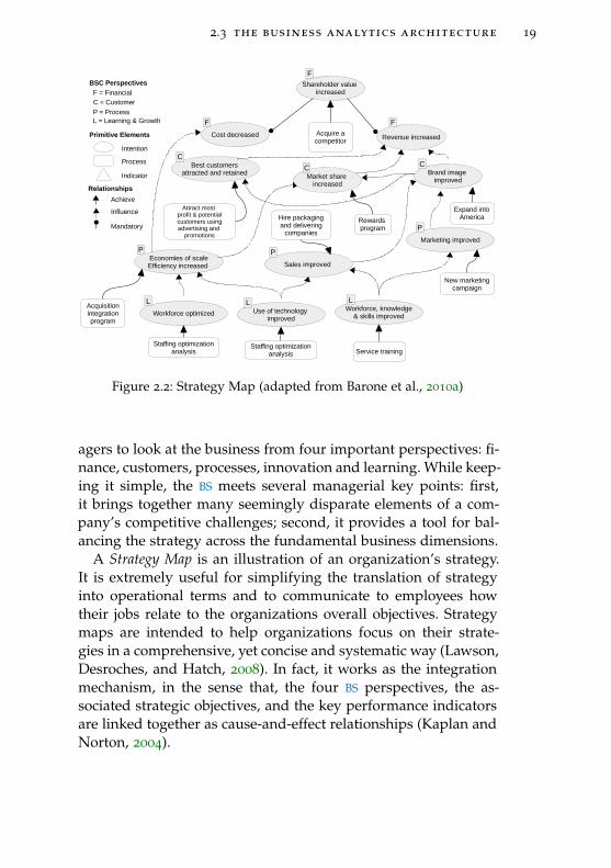
agers to look at the business from four important perspectives: fi-nance, customers, processes, innovation and learning. While keep-ing it simple, the BS meets several managerial key points: first,it brings together many seemingly disparate elements of a com-pany’s competitive challenges; second, it provides a tool for bal-ancing the strategy across the fundamental business dimensions.
A Strategy Map is an illustration of an organization’s strategy.It is extremely useful for simplifying the translation of strategyinto operational terms and to communicate to employees howtheir jobs relate to the organizations overall objectives. Strategymaps are intended to help organizations focus on their strate-gies in a comprehensive, yet concise and systematic way (Lawson,Desroches, and Hatch, 2008). In fact, it works as the integrationmechanism, in the sense that, the four BS perspectives, the as-sociated strategic objectives, and the key performance indicatorsare linked together as cause-and-effect relationships (Kaplan andNorton, 2004).

20 how business analytics should work
The main objective of BPM (Jeston and Nelis, 2008) is to alignthe processes with the business strategy. It essentially pursuesthe “achievement of the organization’s objectives through the im-provement, management and control of essential business pro-cesses”. On the other hand, the Business Process ManagementNotation (BPMN) (Decker et al., 2010) is a notation standard formodeling business processes, probably the best known and estab-lished in the industry. The primary focus of BPM is in elementsand processes, while BS and strategy maps focus on strategy andobjectives.
Therefore, at this architectural level (the semantic layer) wemake use of three different type of models. The strategy map(see Figure 2.2) provides a way to depict a strategy that achieves amain goal (Barone et al., 2010a). A goal is split in several subgoalscreating a hierarchy that clearly sets how the subgoals should beaccomplished to achieve the main goal. To attain a particular goal,one or more processes must be performed, and a set of indicatorsare configured to measure the achievement level of every goal keyperformance indicator. Notice that each goal has a label indicat-ing which dimension of BS corresponds to (financial, customer,process, learning & grow).
Within this modeling technique we regard the strategy, the met-rics we are going to use to measure the accomplishment level, thekey processes involved in this accomplishment, and the (causal)relation among these elements. Whereas the strategy componentsare all included in this diagram, not all the business process aredepicted on it. For these other processes that we consider worthto monitor but are not included in the strategy map, we use theBPMN.
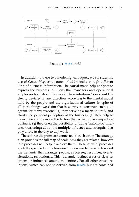
The BPMN express the flow of processes, their relationships andinteractions from the initial state to the final one. We widelyadopt the standard BPMN 2.0 (Decker et al., 2010). This type ofmodels contain information about resources and how are theyconsumed/produced by the processes, as well as detailed infor-mation of each element like geographical location, organizationallevel, starting conditions, processing time. They provide an inter-nal look of the organization, leaving aside the global picture ofstrategic goals.
2.3 the business analytics architecture 21
Analyzecustomer
order
CheckCredit history
CreditFiles Check
InventoryOrder from
supplier
Ship item
ContactCustomer
Company
Place orderProvide card
details
Provide furtherinformation
Receive item
Customer
Credit check
Figure 2.3: BPMN model
In addition to these two modeling techniques, we consider theuse of Causal Maps as a source of additional although differentkind of business information. The causal maps help analysts toexpress the business intuitions that managers and operationalemployees hold about they work. These intuitions/ideas could beclearly deviated in any direction, according to the mental modelhold by the people and the organizational culture. In spite ofall these things, we claim that is worthy to construct such a di-agram for many reasons: (1) they serve as a mean to unify andclarify the personal perception of the business; (2) they help todetermine and focus on the factors that actually have impact onbusiness; (3) they open the possibility of doing ’automatic’ infer-ence (reasoning) about the multiple influence and strengths thatplay a role in the day to day work.
These three diagrams are connected to each other. The strategyplan provides the full map of goals, how they are related, how cer-tain processes will help to achieve them. These ’certain’ processesare fully specified in the business process model, in which we setthe dynamic that arranges people, processes, resources, events,situations, restrictions... This ’dynamic’ defines a set of clear re-lations or influences among the entities. For all other causal re-lations, which can not be derived from BPMN, but are contained

22 how business analytics should work
Relative value
Price of substitutes
Demand
Price
Profits
Cost for production
+ +
+
+
-
- Supply
-
+
Speculativedemand
Expectationof risingprices
New dealers
+
+
+
+
+
B
B
B
R
Figure 2.4: Causal Map
in the knowledge formed by the people’s experience, we use thecausal maps.
The idea behind all this is to represent as much business knowl-edge as we can. It is in this layer where the business conceptsacquire their meanings. It provides a semantic context in whichthe ideas are defined, and constitute the proper environment fordirect interaction with the business user. From the users’ perspec-tive, this new ’semantic environment’ will provide at least twobig benefits. First, they will not be bothered with technical stuff,so they can center at business analysis and decision. Second, theyare not left alone when analyse data: they are supported, guidedand powered by the system, following the logic captured by thediagrams previously introduced.
2.3.2 Mapping Layer - Conceptual Mapping
One of the big challenges that information technology shouldface nowadays is bridging the gap between the ideas or concepts

2.3 the business analytics architecture 23
that humans use everyday, and the data elements that populatethe enormous digital universe. As the society becomes more andmore data-centered, and the data incrementally proliferate everyday, the solution of this challenge gets more and more relevance.
Most of the available data is stored in relational format. It usu-ally consists on a set of data tables, which are related by keys-columns following certain rules. The Entity Relationship Model(Chen, 1976) probably constitute the most well established de-facto standard for storing and representing data, even thoughsome new and very promising approaches have emerged in thelast years (Han et al., 2011).
Many solutions have been proposed to close the representa-tional gap between the storage layer (e.g., Entity RelationshipModel) and the conceptual layer, which gives the ’user-semantic’meaning to the data. Some of them include Hibernate, Doctrine,RedBean, ActiveRecord. These mapping technologies are knownas Object-Relational Mappings.
However, for BA applications these approaches are insufficientdue to the huge volume of data involved. For a mid-size foodcompany, it is not rare to handle 100 thousands billing transac-tions a day. The problems come when the managers and busi-ness users want to make sense of datasets that expand severalyears and interactively explore them, because the underling stor-age technology can not timely support such a huge operations.That’s why the so called Data-Warehouse technologies has cometo existence, as well as the Online Analytical Processing and Data-Marts tools (Lenzerini et al., 2003). They intend to solve the prob-lem by pre-aggregating the data into data-cubes, drastically re-ducing the system response time. In top of this data aggregationlayer it is common to find data visualization tools, constitutingthe ’business intelligence’ capability of such a systems. This kindof systems have become very popular in the ICT industry, but theysuffer some weaknesses. Their implementation usually involveimportant resources in terms of ICT personnel effort and requiredtime; they usually are pretty specific to the concrete industry andcompany involved; and being constructed following a bottom-up methodology, they can grow in size and complexity withoutreal business necessity. For these reasons, some alternatives to

24 how business analytics should work
Day
Weekday
Weekend
x
x
Week
Month
x
x
Year
DayID
DayDate
WeekdayID
Description
WeekendID
Description
WeekID
Description
MonthID
Name
YearID
Description
Day
PK DayKey
DayIDDayDateDayOfWeek
FK1 WeekFK1 Month
WeekMonth
PK WeekIDPK MonthID
MonthNameFK1 Year
Year
PK YearKey
Description
Figure 2.5: Conceptual Mapping excerpt
Data-warehousing have been proposed. Some of them primarilyfocus on hardware optimization, like ’In-memory’ technologies(Plattner, 2009). Other approaches to solve the gap between theconceptual and the storage facets of data, are based on concep-tual modeling techniques. They help to raise the abstraction level,seamlessly connecting user’s concepts with physical data.
The second layer of our Business Intelligence Architecture isthe Conceptual Mapping, which is responsible of mapping thebusiness concepts to the raw-data entities. Our approach is par-tially based on the Conceptual Integration Model proposed byRizzolo et al. (2010). They extend MultiDim model (Malinowskiand Zimányi, 2008), which in turn extends Chen’s Entity Rela-tionship Model model to support multidimensionality.
2.3.3 Data Layer - Data-Warehouses
Data are proliferating in volume and format, they are presentthroughout the organizations. Many data storage solutions have

2.3 the business analytics architecture 25
appeared in the last years, so companies usually combine manyof them. This layer is responsible for unifying all enterprise datasources available, in such a way it is possible to connect themwith the Conceptual Mapping layer. We widely adopt ETL indus-try standard to this purpose, in addition to data warehousingtechnologies.
Data warehouses typically contain data from multiple organi-zational silos. This data is often more integrated, better under-stood, and cleansed more thoroughly. However, for building pre-dictive analytic models they hide some drawbacks, as the prob-lem of eliminating critical outlier data within the process of datacleansing. Despite this, data warehouses can be very useful forthe construction of predictive analytic models, if built correctly.Doing so, you will regard at least the following tips (Taylor, 2011):(1) Data warehouses are not as space-constrained as operationaldatabases, and mostly are used for historical analysis. As such,there is less pressure to delete unused records. So maintain asmuch data as you can. (2) The ability to store more data makesit more practical to store a new version of the record every timeit is updated in the source system. It will avoid leaks from thefuture. (3) Many data warehouses are used to produce reportsand analysis at a summary level. Taking wide profit of predictiveanalytic models imply storing transactional data as well as theroll-up and summary data. A well designed and implementeddata warehouse is a great source of data that leverage the powerof predictive analytics.
Trying to gather in a single system all the information of acompany, could become an arduous task, and sometimes imprac-tical due to the volume of data involved. For that reason, someorganizations have developed what has become to called datamarts: data is extracted from operational databases of from anenterprise data warehouse and organized to focus on a particu-lar solution area. Owned by a single department of business area,data marts allow a particular group of user more control and flex-ibility when it comes to the data they need.
Another less common extension of data warehouses consist ofconnecting them with unstructured sources of data, like the Web,written documents, and any other media like images, audio and

26 how business analytics should work
Marketing
POS
ERP
CRM
...
Operational Systems
ODS
Staging Area
Integration Layer
Data Vault
Data Warehouse Mart
Mart
Mart
Mart
Data Marts
Mart
Mart
Mart
Mart
ETL
ETL
ETL
ETL
ETL
Audio
Video
WWW
Text
...
Multimedia Data Filters
ETL
ETL
Mart
Mart
Mart
Mart
Data Marts
Mart
Mart
Mart
Mart
ETL
Figure 2.6: Basic components of a Data Warehouse
video. To do so, it is necessary to configure and specify how theraw data is transformed into regular data, what is the valid out-put range and what to do if something is wrong. This work isdone by separated modules that we call Multimedia Data Filters.Basically a Multimedia Data Filters receive a source media like avideo and return a corresponding bunch of data. They focus ona particular type of source media and are powered by analytics,and need to be specify separately due to the involved complexity.Some example are sentiment analysis, web mining, video analy-sis and image decomposition.
2.4 analytical foundations
As we have already mentioned, at every level in the process of ab-straction we take profit of analytical algorithms. They are usuallygathered under the names of Pattern Recognition and MachineLearning algorithm, but it is not unusual to hear about ArtificialIntelligence, Data Mining and Knowledge Discovery. What areall they really about?

2.4 analytical foundations 27
Pattern Recognition deals with the problem of (automatically)finding and characterising patterns or regularities in data (Shawe-Taylor and Cristianini, 2004). By patterns we understand any re-lations, regularities or structure inherent in a source of data. Bydetecting patterns, we can expect to build a system that is able tomake predictions on new data extracted from the same source. Ifit works well, we say that the system has acquired generalizationpower by learning something from the data.
This approach is commonly called the learning methodology, be-cause the process is focused on extracting patterns from the sam-ple data that lead us to make generalizations about the popula-tion data (Villegas, 2013). In this sense, it is a data driven approach,in contrast with theory driven approach. However, it is extremelyuseful to tackle complex problems in which an exact formula-tion is not possible, for example, recognising a face in a photo orgenes in a DNA sequence.
Consider a dataset containing thousands of observations of peaplants, in the same format of Gregor Mendel’s observations. It isobvious that the characters (color and size, for example) of certainpea plant generation could be predicted by using the Mendel’slaws. Therefore, the dataset contains an amount of redundancy,that is, information that could be reconstructed from other partsof the data. In such cases we say that the dataset is redundant.
This characteristic has an special importance for us, becausethe redundancy in the data leads us to formulate relations ex-pressing such behaviours. If the relation is accurate and holds forall observations in the data, we refer to it as an exact relation. Thisis the case, for example, of the Laws of Inheritance: Mendel foundthat some patterns surprisingly held for all his experiments. Forthat reason, we say that this part of the data is also predictable: wecan reconstruct it from the rest of the data, as well as predictingfuture data, like the color and size of new plants by using thecurrent plants data.
Finding exact relations is not, by far, the general case for some-one who analyses data. Certainly, the common case is findingpatterns that hold with a certain probability. We call them statisti-cal relations. Examples of such relations are: forecasting the totalsales of a company for the next month, or inferring the credit

28 how business analytics should work
score (Huang, Chen, and Wang, 2007) of a new client in a bankby analysing his information.
The science of pattern analysis has considerably evolved fromits early formulations. In the 1960’s efficient algorithms for de-tecting linear relations were introduced. This is the case of thePerceptron algorithm (Rosenblatt, 1957), formulated in 1957. Inthe mid 1980’s a set of new algorithms started to appear, makingpossible for the first time to detect nonlinear patterns. This groupincludes the backpropagation algorithm for multilayer neural net-works and decision tree learning algorithms.
The emergence of the new pattern analysis approach knownas kernel-based methods in mid 1990’s, changed the field of pat-tern analysis towards a new and exciting perspective: the newapproach enabled researchers to analyse nonlinear relations withthe efficiency of linear algorithms via the use of kernel matrices.Kernel-based methods first appeared in the form of SVM, a clas-sification algorithm that quickly gained great popularity in thecommunity for its efficiency and robustness. Nowadays we havea variate and versatile toolbox composed by the algorithms de-veloped by the scientific community during the short live of thisresearch area.

Part II
S TAT E S PA C E M O D E L L I N G

3S TAT E S PA C E M O D E L I N G
3.1 overview
State Space (SS) is a general framework that allows for the treat-ment of many different problems in time series analysis. Althoughit first appeared in the 60’s in the field of engineering, nowadaysit is widely used in a surprisingly large set of different domains,including statistics, econometrics and robotics. One of the mostdistinguishing ideas of the SS approach is that observations (ob-served components) are regarded as made up of different (un-observed) components, each of which is modelled separately asstates. Then the models for the different components are put to-gether to form a single model, named a SS model. Although eachcomponent has its own model, all components are then modelledsimultaneously via the SS model which becomes the basis for theanalysis hereafter. The methodology that emerges from this ap-proach is very flexible and general, to the point that many otheralternative techniques used for time series analysis, like ARIMA
and exponential smoothing models, can be expressed in termsof SS modeling and are considered particular realizations of it.This chapter outlines a compilation of common formulation andderivation of the Equations involved in modeling and estimationstages. Derivations are provided as to a minimal context accord-ing to Durbin and Koopman (2012), where further details can befound.
31
32 state space modeling
3.2 state space formulation
3.2.1 Linear Gaussian systems
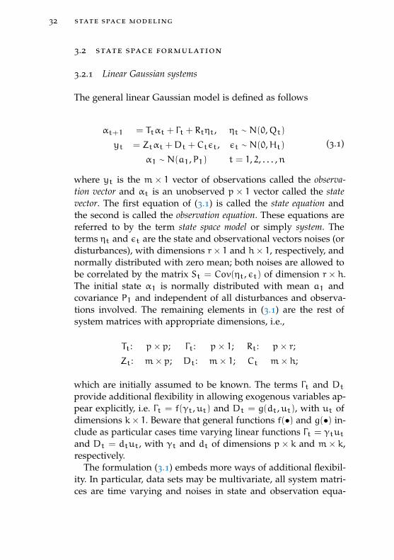
The general linear Gaussian model is defined as follows
αt+1 = Ttαt + Γt + Rtηt, ηt ∼ N(0,Qt)
yt = Ztαt +Dt +Ctεt, εt ∼ N(0,Ht)
α1 ∼ N(a1,P1) t = 1, 2, . . . ,n
(3.1)
where yt is the m× 1 vector of observations called the observa-tion vector and αt is an unobserved p× 1 vector called the statevector. The first equation of (3.1) is called the state equation andthe second is called the observation equation. These equations arereferred to by the term state space model or simply system. Theterms ηt and εt are the state and observational vectors noises (ordisturbances), with dimensions r× 1 and h× 1, respectively, andnormally distributed with zero mean; both noises are allowed tobe correlated by the matrix St = Cov(ηt, εt) of dimension r× h.The initial state α1 is normally distributed with mean a1 andcovariance P1 and independent of all disturbances and observa-tions involved. The remaining elements in (3.1) are the rest ofsystem matrices with appropriate dimensions, i.e.,
Tt: p× p; Γt: p× 1; Rt: p× r;Zt: m× p; Dt: m× 1; Ct m× h;
which are initially assumed to be known. The terms Γt and Dtprovide additional flexibility in allowing exogenous variables ap-pear explicitly, i.e. Γt = f(γt,ut) and Dt = g(dt,ut), with ut ofdimensions k× 1. Beware that general functions f(•) and g(•) in-clude as particular cases time varying linear functions Γt = γtutand Dt = dtut, with γt and dt of dimensions p× k and m× k,respectively.
The formulation (3.1) embeds more ways of additional flexibil-ity. In particular, data sets may be multivariate, all system matri-ces are time varying and noises in state and observation equa-

3.2 state space formulation 33
tions may be correlated. The system is in fact so general that itis not difficult to identify possible redundancies between someterms, and some of them are not strictly necessary in most appli-cations. The counterpart of this approach is the aforementionedflexibility, which makes possible a large set of advanced capabili-ties with minimal effort. Some of these possibilities are exploredin Chapter 4 and exploited in real applications along this thesis.
3.2.2 NonGaussian systems
The non-Gaussian SS set up is shown in Equation (3.2):
αt+1 = Ttαt + Γt + Rtηt, ηt ∼ N(0,Qt)
yt ∼ p(yt | θt) +Dt,
θt = Ztαt t = 1, 2, . . . ,n
(3.2)
Here θt is known as the signal. With this representation it ispossible to deal with three types of models (Durbin and Koop-man, 2012).
1. Exponential family distribution, where p(yt | θt) = exp[y ′tθt−bt(θt) + ct(yt)],−∞ < θt <∞.
2. Stochastic Volatility models, i.e.: yt = exp(12θt)εt +Dt.
3. Observations generated by the relation yt = θt + εt, εt ∼
p(εt), with p(•) being a distribution of the exponential fam-ily.
3.2.3 Nonlinear systems
Finally, the non-linear models are of the type shown in Equation(3.3).
αt+1 = Tt(αt) + Γt + Rt(αt)ηt, ηt ∼ N(0,Qt(αt))
yt = Zt(αt) +Dt +Ct(αt)εt, εt ∼ N(0,Ht(αt))
t = 1, 2, . . . ,n
(3.3)

34 state space modeling
Functions Tt(αt) and Zt(αt) with first derivatives provide non-linear transformations of the state vector into vectors of size p× 1and m × 1, respectively. The rest of system matrices may alsodepend on the state vector and St = 0.
Given this general framework, (extended) Kalman filtering, stateand disturbance smoothing provide the basis for optimal state es-timation, parameter estimation, signal extraction, forecasting, etc.
3.3 the kalman filter and smoother
Once a model is put into SS form, the KF can be employed to com-pute optimal forecasts of the mean and covariance matrix of thenormally distributed state vector αt+1, based on the available in-formation through time t. This section outlines the filtering andsmoothing algorithms that may be used in a SS context.: filteringbases an inference about the state vector only on the informationup to time t; smoothing incorporates the full set of informationin the sample, where one distinguishes between state smoothingand disturbance smoothing. Subsection §3.3.4 shows how the KF
deals with missing observations, which serves as a basis for thesubsequent outline of using the KF for forecasting purposes. Thecorrection of the previous algorithms to tdeal with exact initial-ization of the KF and smoothers will be discussed in §3.3.6.
3.3.1 Filtering
In this section we shall derive the appropriate formulae to esti-mate the state vector αt for the case of linear Gaussian SS modelformulated in Equation (3.1) with St = 0.
We begin with a series of observations Yt = (y1,y2, . . . yn). LetYt−1 the set of past observation y1, . . . ,yt−1. Our objective is to

3.3 the kalman filter and smoother 35
obtain the conditional distributions of αt and αt+1 given Yt fort = 1 . . . n. This leads us to define the following variables:
at|t = E(αt|Yt)
at+1 = E(αt+1|Yt)
Pt|t = Var(αt|Yt)
Pt+1 = Var(αt+1|Yt)
(3.4)
Since all involved variables are normally distributed, the con-ditional distributions of any subset of these variables are alsonormal, and the distributions of αt and αt+1 given Yt are there-fore given by
αt ∼ N(at|t,Pt) (3.5)
αt+1 ∼ N(at+1,Pt+1) (3.6)
At this point we need to derive the recursive expression to cal-culate at|t, at+1, Pt|t, Pt+1 from at and Pt for t = 1, . . . ,n. Withthis in mind, let define what is called the one-step ahead forecasterror of yt given Yt−1:
vt = yt − E(yt|Yt−1)
= yt − E(Ztαt +Dt +Ctεt|Yt−1)
= yt −Ztat −Dt
(3.7)
Since vt is the part of yt that cannot be predicted from thepast, the vt’s are usually referred to as innovations, which has aexpected value of zero,
E(vt|Yt−1) = E(yt −Ztat −Dt|Yt−1)
= E(Ztαt +Dt +Ctεt −Ztat −Dt|Yt−1)
= 0
(3.8)
and Cov(yj, vt) = E[yjE(vt|Yt−1)′] = 0 for j = 0, . . . , t− 1. Once
we have got Yt−1, vt can be conceived as the additional bit ofinformation provided by the new datapoint yt to form Yt. We

36 state space modeling
therefore state that having Yt−1 and vt fixed, Yt is also fixed,which leads us to state:
at|t = E(αt|Yt) = E(αt|Yt−1, vt)
at+1 = E(αt+1|Yt) = E(αt+1|Yt−1, vt).(3.9)
This derivation gives us the appropriate context to apply the re-gression Lemma 1 on which most KF derivations rely. The regres-sion lemma is defined as follows:
Lemma 1 The conditional distribution of x given y is normal withmean vector
E(x|y) = µx + ΣxyΣ−1yy(y− µy) (3.10)
and variance matrix
Var(x|y) = Σxx − ΣxyΣ−1yyΣ
′xy. (3.11)
Taking x and y as αt and vt in Equation (3.9), respectively:
at|t = E(αt|Yt−1) +Cov(αt, vt)[Var(vt)]−1vt, (3.12)
where Cov and Var refer to conditional covariance and varianceof the joint distribution of αt given vt and Yt−1. Digging a bitdeeper into these two quantities we obtain
Cov(αt, vt) = E[αt(Ztαt +Dt +Ctεt −Ztat −Dt)′|Yt−1]
= E[αt(αt − at)′Z ′t|Yt−1]
= PtZ′t,
(3.13)
and
Ft = Var(vt|Yt−1)
= Var(Ztαt +Dt +Ctεt −Ztat −Dt|Yt−1)
= ZtPtZ′t +CtHtC
′t
(3.14)
3.3 the kalman filter and smoother 37
In consequence, we can restate Equation (3.12) as
at|t = at + PtZ′tF
−1t vt. (3.15)
Applying the same procedure to Var(αt|Yt) and the same Lemma1 we obtain:
Pt|t = Var(αt|Yt)
= Var(αt|Yt−1, vt)
= Var(αt|Yt−1) −Cov(αt, vt)[Var(vt)]−1Cov(αt, vt) ′
= Pt − PtZ′tF
−1t ZtP
′t
(3.16)
which is fully computable assuming Ft nonsingular. By the mo-ment we have obtained what is called the updating step of the KF,specifically with the relations (3.15) and (3.16).
Now we derive recursions for at+1 and Pt+1. We start fromEquations (3.4) and proceed as follows
at+1 = E(αt+1|Yt)
= E(Ttαt + Γt + Rtηt|Yt)
= TtE(αt|Yt) + Γt
= Ttat|t + Γt
= Ttat + TtPtZ′tF
−1t vt + Γt
= Ttat +Ktvt + Γt
(3.17)
by substituting at|t from Equation (3.15) and taking
Kt = TtPtZ′tF
−1t . (3.18)
38 state space modeling
The matrix Kt is widely known as the Kalman gain. Proceeding insimilar way for Pt+1 and substituting from (3.16) and (3.18) weobtain
Pt+1 = Var(αt+1|Yt)
= Var(Ttαt + Γt + Rtηt|Yt)
= TtPt|tT′t + RtQtR
′t
= Tt[Pt − PtZ′tF
−1t ZtP
′t]T′t + RtQtR
′t
= TtPtT′t − TtPtZ
′tF
−1t ZtP
′tT′t + RtQtR
′t
= TtPtT′t −KtZtP
′tT′t + RtQtR
′t
= TtPt(Tt −KtZt)′ + RtQtR ′t.
(3.19)
Equations (3.17) and (3.19) are called the prediction equations ofthe KF.
3.3.1.1 Kalman filter recursion
We collect together the filtering equations obtained so far
vt = yt −Ztat −Dt Ft = ZtPtZ′t +CtHtC
′t
at|t = at + PtZ′tF
−1t vt Pt|t = Pt − PtZ
′tF
−1t ZtP
′t
at+1 = Ttat|t + Γt Pt+1 = TtPt|tT′t + RtQtR
′t,
(3.20)
for t = 1, . . . ,n, considering α1 ∼ N(a1,P1) as the initial statevector and Kt = TtPtZ ′tF
−1t .
3.3.1.2 Steady state
In the case of a time-invariant system, i.e., the matrices Tt,Zt, Γt,Dt, Rt, Ct, Qt and Ht are constant over time, the KF recursionfor the term Pt+1 converges to a constant matrix P that has thisform
P = TPT ′ − TPZ ′F−1ZPT ′ + RQR ′, (3.21)
with F = ZPZ ′ + CHC ′. The steady state solution of the KF is theone obtained after convergence of P as been stated. The computa-tional savings derived from using steady state after convergenceare very high because the recursive computation of Ft,Kt,Pt|tand Pt+1 are not required anymore.

3.3 the kalman filter and smoother 39
3.3.1.3 State estimation errors and forecast errors
Denote the state estimation error as
xt = αt − at, (3.22)
with Var(xt) = Pt. From the filtering equations (3.20) and thedefinition of xt we can derive the following quantities
vt = yt −Ztat −Dt
= Ztαt +Dt +Ctεt −Ztat −Dt
= Ztxt +Ctεt,
(3.23)
and
xt+1 = αt+1 − at+1
= Ttαt + Γt + Rtηt − (Ttat +Ktvt + Γt)
= Ttxt + Rtηt −KtZtxt −KtCtεt
= Ltxt + Rtηt −KtCtεt
(3.24)
where Lt = Tt−KtZt. Then, we can obtain the innovation analogueof the SS model, which has the following form
vt = Ztxt +Ctεt
xt+1 = Ltxt + Rtηt −KtCtεt(3.25)
with x1 = α1 − a1. The recursion for Pt+1 can be derived by thesteps
Pt+1 = Var(xt+1)
= E[(αt+1 − at+1)x′t+1]
= E(αt+1x′t+1)
= E[(Ttαt + Γt + Rtηt)(Ltxt + Rtηt −Ktεt)′]
= TtPtL′t + RtQtR‘t
(3.26)
since Cov(xt,ηt) = 0.
40 state space modeling
3.3.2 State smoothing
In the previous section we derived the conditional density of αtgiven the information known up to time t, that is y1, . . . ,yt. Thisled us to the celebrated KF recursion, which can be seen as a for-ward process. In this section we shall derived conditional densityof αt given the entire series y1, . . . ,yn. We will see that in thiscase formulation suggests a backward iterative process. Again weproceed by assuming normality and using Lemma 1.
Our objective is to obtain the conditional mean αt = E(αt|Yn)and the conditional variance matrix Vt = Var(αt|Yn) for t =
1, . . . ,n. As in the previous section, we build on to the assump-tion that α1 ∼ N(a1,P1) where a1 and P1 are known. The consid-eration of the case a1 and P1 unknown are faced following theKF initialization strategy (Durbin and Koopman, 2012, and Sec-tion §3.3.6). The conditional mean E(αt|yt, . . . ,ys) is sometimescalled a fixed interval smoother to state that it is based on the fixedinterval (t, s).
Consider the innovations v1, . . . , vn as defined in Subsection§3.3.1.1 and denote the vector vt:n = (v ′t, . . . , v
′n)′. To calculate
E(αt|Yn) and Var(αt|Yn) we apply Lemma 1 using the fact thatYn is fixed when Yt−1 and vt:n are fixed, and that vt, . . . , vnare independent of Yt−1 and each other with zero mean. SinceE(αt|Yt−1) = at for t = 1, . . . ,n we therefore can state
αt = E(αt|Yn) = E(αt|Yt−1, vt:n)
= at + Σnj=tCov(αt, vj)F
−1j vj,
(3.27)
where Cov refers to covariance in the conditional distributiongiven Yt−1 and Fj is as it is defined in Equation (3.14).
However, it follows from Equation (3.25) that
Cov(αt, vt) = E(αtv′j|Yt−1)
E[αt(Zjxj + εj)′|Yt−1]
E(αtx′j|Yt−1)Z
′j
(3.28)
for j = t, . . . ,n.

3.3 the kalman filter and smoother 41
Moreover,
E(αtx′t|Yt−1) = E(αt(αt − at)|Yt−1) = Pt,
E(αtx′t+1|Yt−1) = E(αt(Ltxt + Rtηt −Ktεt)
′|Yt−1) = PtL′t,
E(αtx′t+2|Yt−1) = PtL
′tL′t+1
...
E(αtx′t+n|Yt−1) PtL
′t . . . L
′n−1
(3.29)
using Equation (3.25) repeatedly for t+ 1, t+ 2, . . . . Substitutinginto Equation (3.28) gives
αn = an + PnZ′nF
−1n vn
αn−1 = an−1 + Pn−1Z′n−1F
−1n−1vn−1 + Pn−1L
′nZ′nF
−1n vn
αt = at + PtZ′tF
−1t vt + PtL
′tZ′t+1F
−1t+1vt+1
+ · · ·+ PtL ′t . . . L ′n−1Z′nF
−1n vn
(3.30)
for t = n− 2,n− 3, . . . , 1. We can therefore express the smoothedstate vector as
αt = at + Ptrt−1 (3.31)
where rn−1 = Z ′nF−1n vn, rn−2 = Z ′n−1F
−1n−1vn−1+L
′n−1Z
′nF
−1n vn
and
rt−1 = Z ′tF−1t vt + L
′tZ′t+1F
−1t+1vt+1+
· · ·+ L ′tL ′t+1 · · ·+ L′n−1Z
′nF
−1n vn
(3.32)
for t = n− 2,n− 3, . . . , 1. The vector rt−1 is a weighted sum ofinnovations vj occurring after time t− 1, that is, for j = t, . . . ,n.Doing the appropriate substitutions we obtain the backwards re-cursion
rt−1 = Z ′tF−1t vt + L
′trt (3.33)

42 state space modeling
for t = n, . . . , 1, with rn = 0. Collecting these results togethergives the recursion for state smoothing,
αt = at + Ptrt−1,
rt−1 = Z ′tF−1t vt + L
′trt
(3.34)
for t = n, . . . , 1 with rn = 0.The smoothed state variance matrix Vt = Var(αt|Yn) can be
obtained by applying Lemma 1 to the conditional joint distribu-tion of αt and vt:n given Yt−1. The resulting recursion is
Nt−1 = Z ′tF−1t Zt + L
′tNtLt,
Vt = Pt − PtNt−1Pt(3.35)
and can be used to compute Vt for t = n . . . 1 with Nn = 0. SeeDurbin and Koopman (2012) for derivation details.
3.3.3 Disturbance smoothing
The disturbance smoother may be used when an estimation ofthe noises in the SS system are required, typically for model vali-dation. It deals with computing εt = E(εt|Yn) and ηt = E(ηt|Yn)of the disturbance vectors εt and ηt given all the observationsy1, . . . ,yn. By Lemma 1 we have
εt = E(εt|Yt−1, vt, . . . , vn)
= Σnj=tE(εtv′j)F
−1j vj
(3.36)
for t = 1, . . . ,n, since E(εt|Yt−1) = 0 and εt and vt are jointly in-dependent of Yt−1. It follows from Equation (3.25) that E(εtv ′j) =E(εtx
′j)Z′j + E(εtx
′t) = 0 for t = 1, . . . ,n and j = t, . . . ,n. There-
fore
E(εtv′j) =
Ht, j = t
E(εtx′j)Z′j, j = t+ 1, . . . ,n,
(3.37)
3.3 the kalman filter and smoother 43
with
E(εtx′t+1) = −HtK
′t,
E(εtx′t+2) = −HtK
′tL′t+1,
...
E(εtx′t+n) = −HtK
′tL′t+1 · · ·L
′n−1,
(3.38)
for t = 1, . . . ,n− 1. Now we can restate Equation (3.36) as
εt = Ht(F−1t vt −K
′tZ′t+1F−1t+1vt+1 − · · ·
−K ′tL′t+1Z
′t+2F
−1t t+ 2vt+2 −K
′tL′t+1 · · ·L
′n−1Z
′nF
−1n vn)
= Ht(F−1vt −K
′trt)
(3.39)
To derive ηt we proceed analogously to (3.36). We have
ηt = Σnj=tE(ηtv′j)F
−1j vj, (3.40)
for t = 1, . . . ,n. Using Equation 3.25 we can state that
E(ηtv′j) =
QtR ′tZ ′t+1, j = t+ 1
E(ηtx′j)Z′j, j = t+ 2, . . . ,n
(3.41)
After some algebra manipulation the recursion simplifies toηt = QtR
′trt.
The corresponding smoothed disturbance variance matrices areobtained similarly as Equation (3.35) resulting in
Var(εt|Yn) = Ht −Ht(F−1t +K ′tNtKt)Ht,
Var(ηt|Yn) = Qt −QtR′tNtRtQt
(3.42)
for t = n, . . . , 1 where Nn = 0. Derivations details are availablefrom Durbin and Koopman (2012).

44 state space modeling
3.3.4 Missing observations
Within the SS framework, missing observations can be easily dealtwith. Durbin and Koopman (2012) show that for a missing setof observations the original filter and smoothing recursions canbe used for all t. The one-step ahead forecast error vt and theKalman gain matrix Kt are simply set to zero for all missing datapoints. With vt = 0 and Kt = 0 the filter recursions in (3.20)become
at+1 = Ttat + Γt,
Pt+1 = TtPtT′t + RtQtR
′t,
(3.43)
The smoothing recursions in (3.34) can be written as
rt−1 = T ′trt,
Nt−1 = T ′tNtTt,(3.44)
while the other relevant smoothing steps remain unaffected.
3.3.5 Forecasting
The discussion related to missing observations serves as a basis touse the KF for forecasting purposes. Given the vector observationsy1, . . . , yn, the objective is to generate the forecasts for yn+j forj = 1, . . . , J. Let yn+j be the minimum Mean Squared Error (MSE)forecast given Yn, i.e. yn+j has a minimum MSE matrix
Fn+j = E((yn+j − yn+j)(yn+j − yn+j)′|Yn) (3.45)
for all yn+j. Given the standard result that E((X− λ)(X− λ) ′) isminimized for λ = µ, where µ is the mean of a random variable X,it follows immediately that the conditional mean of yn+j givenYn represents the minimum MSE forecast:
yn+j = E(yn+j|Yn) (3.46)

3.3 the kalman filter and smoother 45
From observation Equation (3.1) we have yn+j = Zn+jαn+j +
Dn+j +Cn+jεn+j, and therefore
yn+j = Zn+jE(αn+j|Yn) +Dn+j
= Zn+jan+j +Dn+j(3.47)
with conditional MSE matrix
Fn+j = Zn+jPn+jZ′n+j +Cn+jHn+jC
′n+j (3.48)
Recursions for computing an+j and Pn+j can be derived as
an+j+1 = Tn+jan+j + Γn+j
Pn+j+1 = Tn+jPn+jT′n+j + Rn+jQn+jR
′n+j
(3.49)
which are identical to the KF recursions for an+j and Pn+j in(3.20) with vn+j = Kn+j = 0. As these are the same conditionsthat allow the KF to deal with missing observations in Section§3.3.4, an l-period-ahead forecast, denoted as yn+j, can be calcu-lated routinely by interpreting yn+j, . . . ,yn+J as missing obser-vations and by employing the KF beyond time t = n with vt andKt set to zero (Durbin and Koopman, 2012).
3.3.6 Initialization of filter and smoother
So far the distribution of the initial state vector α1 has been as-sumed to be N(a1, P1), i.e., with known mean and covariance. Inpractice, however, at least some elements of the distribution of α1are unknown. In the literature, at least three ways of initializingnon-stationary SS models are discussed.
The first one is to employ a diffuse prior that fixes a1 at an ar-bitrary value and allows the diagonal elements of P1 to go toinfinity. Following Durbin and Koopman (2012) a general specifi-cation for the initial state vector is given by
α1 = a+Aδ+ R0η0, δ ∼ N(0, κIq) , η0 ∼ N(0, Q0) (3.50)
where the p× 1 vector a can be treated as a zero vector whenevernone of the elements of of α1 are known constants. The p× q
46 state space modeling
matrix A and the p × (p − q) matrix R0 are fixed and knownselection matrices with A ′R0 = 0. The initial covariance matrixQ0 is assumed to be known and positive definite. The q×1 vectorδ is treated as a random variable with infinite variance and iscalled the diffuse vector as κ→∞. This leads to
P1 = P∗ + κP∞ (3.51)
with P∗ = R0Q0R′0 and P∞ = AA ′. With some elements of α1
being diffuse, the initialization of the KF is referred to as diffuseinitialization . However, in cases where P∞ is a nonzero matrix, thestandard KF cannot be employed as no real value can represent κas κ → ∞. It is necessary to find an approximation or to modifythe KF in an appropriate way. Many references, like Harvey (1989),propose to replace κ by a large but finite numerical value, whichenables the use of the standard KF.
The assumption of an infinite variance might be regarded un-natural as all observed time series have a finite variance. Thisleads to the second way of initialization. Rosenberg (1973) con-siders α1 to be an unknown constant that can be estimated fromthe first observation y1 by maximum likelihood. It can be shownthat by this procedure, the same initialization of the filter is ob-tained as by assuming that α1 is a random variable with infinitevariance (Durbin and Koopman, 2012).
As an alternative to the previous methods, Durbin and Koop-man (2012) develop exact initialization techniques when κ → ∞.The first step is to acknowledge that Equation (3.51) may be gen-eralize for every t, i.e., when the state vector is formed by somediffuse variables, the mean square error matrix Pt may be de-composed into a part associated with diffuse elements P∞,t anda part with a proper distribution P∗,t, that is
Pt = P∗,t + κP∞,t (3.52)
The initial P∞,1 is a diagonal matrix with positive values in thepositions where the states are diffuse, and zeros in the remainder.The trick then consists of splitting the KF into two parts by ex-panding the inverse of Ft = κF∞,t + F∗,t +O(κ−2) in κ−1, whereF∞,t is assumed to be either singular or nonsingular. There is a

3.3 the kalman filter and smoother 47
transient in which P∞,t has some non zero elements, but aftersome iterations it converges to zero in most cases. When this ma-trix collapses to zero the standard KF may be run. The KF with ex-act initialization then splits into two cases, depending on whetherF∞,t is singular or nonsingular (see proofs in Durbin and Koop-man, 2012). The KF with exact initialization is somewhat morecomplicated, i.e.,
vt = yt −Ztat −Dt
F∞,t = ZtP∞,tZ′t
K∞,t = P∞,tZ′tF
−1∞,t
F∗,t = ZtP∗,tZ ′t +CtHtC′t
K∗,t = (P∗,tZ ′t −K∞,tF∗,t)F−1∞,t
P∞,t|t = P∞,t −K∞,tF∞,tK′∞,t
P∞,t = TtP∞,t|tT′t
P∗,t|t = P∗,t −K∞,tZtP′∗,t −K∗,tZtP
′∞,t
P∗,t = TtP∗,t|tT′t +CtHtC
′t
at|t = at +K∞,tvt
at+1 = Ttat|t + Γt
(3.53)
with F∞,t nonsingular. When F∞,t is singular K∞,t does not existand all the previous recursions affected with subindex (∞) do notapply. The filter reduces to applying the standard KF, or in otherwords,
vt = yt −Ztat −Dt
F∗,t = ZtP∗,tZ ′t +CtHtC′t
K∗,t = P∗,tZ ′tF−1∗,t
at|t = at +K∗,tvt P∗,t|t = P∗,t −K∗,tZtP ′∗,t
at+1 = Ttat|t + Γt P∗,t = TtP∗,t|tT′t +CtHtC
′t
(3.54)
In the same way as the KF, finding the optimal smoothed esti-mates of states and covariance matrices with exact initialization
48 state space modeling
involves additional recursive equations. Assuming the filter col-lapsed at time t = d, i.e., P∞,t = 0 for t > d, the smoothingequations are the standard ones in Section §3.3.2. But the recur-sions become more complicated when t 6 d, and, once more, adistinction ought to be done depending on whether F∞,t is sin-gular or not. For F∞,t nonsingular the backwards recursions are
r(1)t−1 = Z ′tF
(1)t vt + L
′tr
(1)t + L
(1) ′
t rt
rt−1 = L ′trt
N(2)t−1 = Z ′tF
(2)t Zt + L
′tN
(2)t Lt + L
′tN
(1)t L
(1)t
+L(1) ′
t N(1)t Lt + L
(1) ′
t NtL(1)t
N(1)t−1 = Z ′tF
(1)t Zt + L
′tN
(1)t Lt + L
(1) ′
t NtLt
Nt−1 = L ′tNtLt
αt = at + Ptrt−1 + P∞,tr(1)t−1
Vt = Pt − PtNt−1Pt − (P∞,tN(1)t−1Pt)
′ − P∞,tN(1)t−1Pt
−P∞,tN(2)t−1P∞,t
(3.55)
In the case of singular F∞,t the recursions are
r(1)t−1 = T ′tr
(1)t
rt−1 = Z ′tF−1t vt + L
′trt
N(2)t−1 = T ′tN
(2)t Tt
N(1)t−1 = T ′tN
(1)t Tt
Nt−1 = Z ′tF−1t Zt + L
′tNtLt
(3.56)
and the backward recursions for αt and Vt remain the same.
3.4 nonlinear and non-gaussian models
In this section we present a compact discussion of the treatmentof nonlinear and non-Gaussian models. We start with the Ex-tended KF in Section §3.4.1 which is a particular way of deal-ing with nonlinear SS models in Section §3.2.3. Importance sam-pling, briefly summarized in Section §3.4.2, constitutes the basis
3.4 nonlinear and non-gaussian models 49
on which Non-Gaussian models may be treated in a SS context. Itallows for the consideration of general density distribution func-tions to characterize the observation term yt ∼ p(yt|αt) and thedisturbances ηt and εt.
3.4.1 The Extended Kalman Filter
The extended KF was developed by Stanley Schmidt at the NASAAmes Research Center for use in a non-linear navigation prob-lem. It is based on the idea of linearising the transitions and ob-servation equations around the most current estimate of the stateand then applying the linear KF to the linearised model. For con-venience we reproduce here the nonlinear model considered inSection §3.2.3:
αt+1 = Tt(αt) + Γt + Rt(αt)ηt, ηt ∼ N(0,Qt(αt))
yt = Zt(αt) +Dt +Ct(αt)εt, εt ∼ N(0,Ht(αt))
t = 1, 2, . . . ,n
(3.57)
Here we consider that Zt(αt), Tt(αt),Rt(αt) and Ct(αt) aredifferentiable functions of αt. If we define
Zt =∂Z(x)∂x ′ |x=at , Tt =
∂T(x)∂x ′ |x=at|t (3.58)
then the first order Taylor expansion of the functions involved inEquation (3.3) are given by
Zt(αt) = Zt(at) + Zt(αt + at) + . . . ,
Tt(αt) = Tt(at|t) + Tt(αt + at|t) + . . . ,
Rt(αt) = Rt(at|t) + . . . ,
Ct(αt) = Ct(at|t) + . . . ,
Ht(αt) = Ht(at) + . . . ,
Qt(αt) = Qt(at|t) + . . .
(3.59)
50 state space modeling
Using at and at|t accordingly as the base for expansion tothe most recent state estimates available when the linearisation isrequired to compute the linear filter equations.
αt+1 ≈ Tt(at|t) + Tt(αt − at|t) + Γt + Rt(αt)ηt
yt ≈ Zt(at) + Zt(αt − at) +Ct(αt)εt(3.60)
where εt ∼ [0,Ht(at)] and ηt ∼ [0,Qt(at|t)].Since this approximation is linear in αt, the basic KF with mean
adjustment can be applied, resulting in the following equations
vt = yt −Zt(at) −Dt
Kt = TtPtZ′tF
−1t Ft = ZtPtZ
′t +Ht(at)
at|t = at + PtZ′tF
−1t vt, Pt|t = Pt −KtFtK
′t
at+1 = Tt(at|t) + Γt Pt+1 = TtPt|tT′t +CtHtC
′t
(3.61)
which comprise the extended KF for the non-linear SS model 3.3.The extended filter is widely used in location tracking and naviga-tion applications. The method is a straightforward modificationto the basic KF, with little additional computational or theoreticalburden. In that sense, exact initialization of the extended versionand extended smoothing is possible along the lines of Section§3.3.6, see Koopman and Lee (2009).
However, the extended KF has a number of known drawbacks.In practice, when model non-linearities are severe, the filter canbecome unstable and diverge from the true state position aftersome iterations. From a functional perspective, a first order ap-proximation can be quite crude. In probabilistic terms, the es-timates are clearly biased, since E(f(X)) 6= f(E(X)) in general.Nonetheless, when the non-linearities in the model are modest,it is a simple and effective means to estimate the state. It em-phasizes the value of the state (in physical applications often thelocation of some object) rather than its probability distribution.

3.4 nonlinear and non-gaussian models 51
3.4.2 Importance sampling
Importance sampling is a general technique for estimating prob-ability distributions when only samples from some other relateddistribution can be generated. It was introduced by Marshall(1956) and appeared first in the econometrics literature in Kloekand Van Dijk (1978). Specializations to non-linear SS models asdescribed in this chapter were developed by Sheppard and Pitt(1997) and Durbin and Koopman (2012).
The basis of Monte Carlo integration methods is that integralsof the form
I =
∫x(α)p(α)dα (3.62)
where p > 0 and∫p(α)dα = 1 can be interpreted as the expecta-
tion of a function x of a random variable which has probabilitydensity p . The law of large numbers asserts the convergence of(functions of) the sample average of observations drawn from thedensity to (functions of) its expectation. This justifies approximat-ing the integral I by drawing N random samples α(i) from p andcalculating the average
1
N
N∑i=1
x(α(i)) (3.63)
Often there is no known method to draw samples from p . How-ever, if an importance density g is available from which samplescan be generated, and g is a reasonable approximation of p , theintegral can be calculated as
I =
∫x(α)
p(α)
g(α)g(α)dα (3.64)
The approximation of x(α) is then performed by drawing sam-ples α(i) from the distribution associated with g and calculatingthe average
1
N
N∑i=1
x(α(i))w(α(i)) (3.65)

52 state space modeling
where
w(α(i)) =p(α(i))
g(α(i))(3.66)
are known as the importance weights.In SS models, we seek to estimate the expectation and other
statistics of the state α conditional on observations y = (y ′i, . . . ,y′n).
In non-linear models, it is generally unknown how to sample di-rectly from p(α|y) . The main problem when we wish to use im-portance sampling is to find an approximating density g(α|y) ,which resembles p(α|y) and from which we can draw samples.The estimates can then be calculated as outlined above.
3.5 maximum likelihood estimation
Running all the recursive algorithms assumes that all system ma-trices are known. However, in real situations this is very rarelythe case. Therefore, prior to the application of these algorithms,estimation of the unknown parameters should be carried out.There are many ways to do this task, of which Exact MaximumLikelihood (ML) in time domain via error decomposition is veryoften preferred, because of its good statistical properties in verygeneral situations (Durbin and Koopman, 2012; Harvey, 1989;Taylor et al., 2007).
The Gaussian log-likelihood function obtained via predictionerror decomposition of the linear SS model is (Durbin and Koop-man, 2012)
logL(ψ) = −mn
2log 2π−
1
2
n∑t=1
(log∣∣∣Ft∣∣∣+ v ′tF−1t vt
)(3.67)
In this equation vt and Ft are the innovations and their vari-ance, respectively, that are naturally obtained by running the KF
on the SS model. This function cannot be used as it is becauseit depends on initialization issues. In the case of a diffuse priorwith d diffuse elements in the initial state vector, the first d time
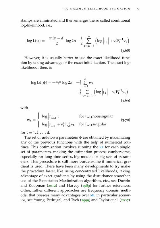
3.5 maximum likelihood estimation 53
stamps are eliminated and then emerges the so called conditionallog-likelihood, i.e.,
logL(ψ) = −m(n− d)
2log 2π−
1
2
n∑t=d+1
(log∣∣∣Ft∣∣∣+ v ′tF−1t vt
)(3.68)
However, it is usually better to use the exact likelihood func-tion by taking advantage of the exact initialization. The exact log-likelihood, then, is
logLd(ψ) = −mn2 log 2π −12
d∑t=1
wt
−12
n∑t=d+1
(log∣∣∣Ft∣∣∣+ v ′tF−1t vt
)(3.69)
with
wt =
log∣∣∣F∞,t
∣∣∣ , for F∞,tnonsingular
log∣∣∣F∗,t∣∣∣+ v ′tF−1∗,t vt, for F∞,tsingular
(3.70)
for t = 1, 2, . . . ,d.The set of unknown parameters ψ are obtained by maximizing
any of the previous functions with the help of numerical rou-tines. This optimization involves running the KF for each singleset of parameters, making the estimation process cumbersome,especially for long time series, big models or big sets of param-eters. This procedure is still more burdensome if numerical gra-dient is used. There have been many developments to try makethe procedure faster, like using concentrated likelihoods, takingadvantage of exact gradients by using the disturbance smoother,use of the Expectaton Maximization algorithm, etc., see Durbinand Koopman (2012) and Harvey (1989) for further references.Other, rather different approaches are frequency domain meth-ods, that possess many advantages over ML in particular scenar-ios, see Young, Pedregal, and Tych (1999) and Taylor et al. (2007).

54 state space modeling
3.6 further issues
As might be expected, many more issues have to be left out ofthis thesis, simply because of space constraints. These may beconsulted in many references in this thesis and references therein.The main ones are Harvey (1989) Durbin and Koopman (2012). Anon exhaustive enumeration of these important issues is: diag-nostics or validation of SS models; univariate treatment of multi-variate models; exact initialization of disturbance smoothers; sim-ulation smoothing algorithms; exact initialization via augmentedKalman filtering; second order extended Kalman filters; unscentedKalman filters and smoothers; particle filters; treatment of non-Gaussian models, etc.

4S S PA C E : A T O O L B O X F O R S TAT E S PA C EM O D E L I N G
4.1 sspace versus other software packages
The previous chapter outlined the main theoretical foundationsof the SS systems. That chapter is complemented with this one,which presents a particular implementation of such theoreticaldevelopments in order to make possible the exploitation to thefull of the power of SS methods in practice.
SSpace is a MATLAB toolbox (The MathWorks Inc, 2018) thatprovides a number of routines designed for a general analysis ofSS systems. It combines both flexibility and simplicity, and at thesame time it enhances the power and versatility of SS modelingin a friendly environment. The toolbox possesses very distinctproperties to other SS pieces of software, but at the same timetakes advantage of methods and algorithms from other sources,mainly Taylor et al. (2007) and Durbin and Koopman (2012) asit has been unfolded in Chapter 3. The combination of all thesefactors give SSpace a particular flavour.
Popularity of high level programming languages like MATLABhas brought the availability of many free packages with an in-credibly wide range of applications in many research areas. SS
routines are not an exception, and therefore good packages areso widespread nowadays, either as open source or paid versions,that it is impossible to quote even a portion of them. Withoutany intention of being exhaustive, we offer here a list of the mostpopular packages within the academic community. A partial re-view is available in volume 41, 2011 of the Journal of Statistical
55

56 sspace : a toolbox for state space modeling
Software (Commandeur, Koopman, and Ooms, 2011). There areseveral toolboxes written in MATLAB, like toolboxes suppliedwith the core program, but also CAPTAIN (Taylor et al., 2007),SSM (Peng and Aston, 2011), SSMMATLAB (Gómez, 2015) andE4 (Casals et al., 2016). One piece of software widely known isSSfPack (Koopman, Shephard, and Doornik, 2008). Some othersare written either in R (Petris and Petrone, 2011), RATS (Doan,2011), gretl (Lucchetti, 2011), etc. Also, some other, menu-drivenprograms that incorporate SS routines with less flexible program-ming capabilities are STAMP (Koopman et al., 2009), Eviews(Bossche, 2011), SAS (Selukar, 2011), Stata (Drukker and Gates,2011), etc. ECOTOOL is a complementary MATLAB toolbox writ-ten by the same authors for the identification and estimation ofdynamical systems (Pedregal and Trapero, 2012a).
In a broad sense, SSpace provides the user with the most ad-vanced and up-to-date features available in the SS framework,sharing some of these properties with some packages mentionedabove and competing with them. However, some other featuresare specific of this toolbox and will not be found in any of thealternatives.
Regarding statistical issues, the main features of SSpace are:
1. Full multivariate linear and non-linear Gaussian models,and univariate non-Gaussian models are implementable. Inany of these possibilities non-linear, time varying or trans-fer function relations with inputs are possible.
2. The framework is very general in the equations formulationand in the sense that all system matrices are potentiallytime-varying or state-dependent.
3. KF, fixed interval smoothing and disturbance smoothing areimplemented with exact, diffuse or ad-hoc initialisation. Ex-act initialisation in non-linear models is also possible fol-lowing Koopman and Lee (2009).
4. Steady state detection of linear invariant systems.
5. Use of exact score in Maximum Likelihood estimation, whenpossible. Use of numerical gradient is always possible, some-times compulsory.

4.1 intro 57
6. Other estimation procedures apart from Maximum Like-lihood are implemented. The toolbox offers ConcentratedLikelihood and minimization of combinations of severalsteps ahead forecast errors.
7. Kalman filtering and smoothing of multivariate systems arebased on univariate treatment of multivariate systems, seeDurbin and Koopman (2012), pages 155-160.
8. A family of models not used in any of the alternative pack-ages is included, namely the Dynamic Harmonic Regres-sion (DHR). To the best knowledge of the authors, this is thefirst time that a multivariate Seemingly Unrelated DHR isused and implemented. Such model is an extension of theunivariate DHR counterpart, see Young, Pedregal, and Tych(1999) and Subsection §4.3.3.
On the operative side, SSpace is rather flexible and user friendlybecause:
• The toolbox is user-oriented in the sense that a big efforthas been done on the developer side with the aim of sim-plifying usage to the final users. As a consequence, a com-prehensive time series analysis may be performed with fullcontrol over models, parameters and specifications, by us-ing just a few number of functions that follow a simple andfixed calling-standard that is easy to remember (see sectionof worked examples below). One example of this simplic-ity is that just one function (namely SSfilter) is used forfiltering any kind of model, regardless of whether it is lin-ear, non-Gaussian or non-linear, i.e.: the toolbox detects thetype of model and apply the appropriate algorithms in eachcase automatically without any specific intervention of theuser.
• The toolbox is composed of less than thirty functions withnames that have been carefully selected following nemotech-nic rules, so that the user may remember them or easily lookfor their names. There are three groups of functions:

58 sspace : a toolbox for state space modeling
– Core functions (named SS*) which set up the modelsand perform the basic operations of filtering, smooth-ing, forecasting, validating, etc.
– Template functions (Sample*) which help the user toset up the model either in terms of the crude SS systemmatrices or in terms of its specific nature.
– Other helpful functions for easy handling of models,matrices, etc. The main ones are for constraining pa-rameters, building semi-definite covariance matrices,differencing time series, building forecast confidencebands, etc.
• Another key point is that models are directly specified bythe user in a user-coded function written in plain MATLABsyntax. This approach has at least the following advantages:
– Once the model is specified in the user-coded function,the same syntax applies to all sort of models, regard-less of linearity, gaussianity, estimation method, etc.i.e.: the same functions with the same syntax are usedfor estimation, filtering, smoothing, etc. Internally theoperation of the toolbox may be rather different ineach case, but such complexity does not require anyintervention of the user.
– The user-coded function is written following a par-ticular template, that is basically a list of empty val-ues for all the system matrices. The toolbox offers par-ticular templates for a wide range of standard mod-els. These templates may be extended or substitutedby users. Such functions and templates may be ex-tended in many ways. Typically, for complex modelsthe model function has to be extended with the aid ofadditional inputs to the MATLAB function in order todefine the model in SS form.
– The user has full control over his models in a fairlystraightforward manner, e.g.: different specific param-eterizations of the same model are possible, parameterconstraints of any kind may be imposed, non-standard
4.1 intro 59
features of the models may be added (like adding het-eroskedasticity, time varying parameters, non lineareXogenous relations, ...), etc.
• Parameter estimation is carried out by the standard fmin-unc function from the optimization toolbox in MATLAB. Byediting the script optimizer.m the user may tune the opti-misation settings and/or change even the optimizer itself.
In summary, the toolbox is highly configurable and could beextended in several ways. Usually default options for modelingare in place in such a way that a few commands with a few op-tions would produce sensible results, but advanced users maytake advantage of the possibility to configure the toolbox at theirown convenience. For example, they could select different setsof initial parameter values to start estimation in order to find theglobal optimum, build alternative cost functions to log-likelihoodfor parameter estimation based on the output of the KF, try outdifferent optimisation algorithms to search for optimal parame-ters, add templates for models not yet implemented or suggestdifferent versions to the existing ones, build canned functions forstandard model estimation, etc.
Table 4.1 shows some of the main features of most commonsoftware packages. The top block corresponds to toolboxes writ-ten in MATLAB, the rest are developed in other environments.The table highlights several facts: i) exact initialization is presentin most packages, ii) non- linear and non-gaussian models areless common than expected and iii) most packages use MaximumLikelihood estimation as the only estimation method.
Moreover, there are some unique properties of SSpace, as far asthe authors are concerned, like the implementation of multivari-ate DHR models, the implementation of systems by direct spec-ification of the system matrices in a MATLAB function, systemestimation via the minimization of forecast errors several stepsahead, the possibility of systems implementing arbitrary non-linear (and possibly multivariate) relations among inputs andoutputs, the possibility of multiple-input-multiple-output trans-fer functions, and the chance to select an arbitrary minimizer al-gorithm to estimate the models (fminunc as a default).
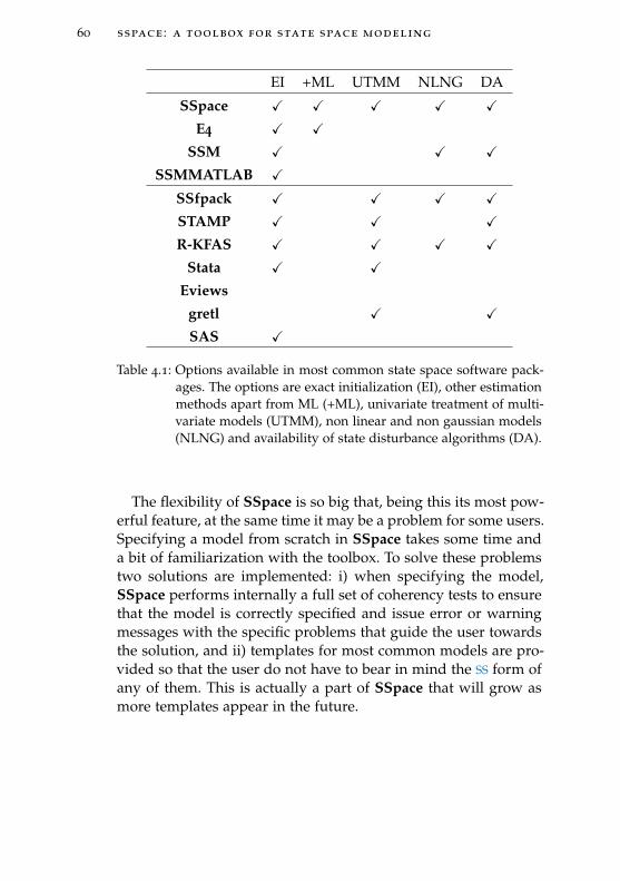
60 sspace : a toolbox for state space modeling
EI +ML UTMM NLNG DA
SSpace X X X X X
E4 X X
SSM X X X
SSMMATLAB X
SSfpack X X X X
STAMP X X X
R-KFAS X X X X
Stata X X
Eviews
gretl X X
SAS X
Table 4.1: Options available in most common state space software pack-ages. The options are exact initialization (EI), other estimationmethods apart from ML (+ML), univariate treatment of multi-variate models (UTMM), non linear and non gaussian models(NLNG) and availability of state disturbance algorithms (DA).
The flexibility of SSpace is so big that, being this its most pow-erful feature, at the same time it may be a problem for some users.Specifying a model from scratch in SSpace takes some time anda bit of familiarization with the toolbox. To solve these problemstwo solutions are implemented: i) when specifying the model,SSpace performs internally a full set of coherency tests to ensurethat the model is correctly specified and issue error or warningmessages with the specific problems that guide the user towardsthe solution, and ii) templates for most common models are pro-vided so that the user do not have to bear in mind the SS form ofany of them. This is actually a part of SSpace that will grow asmore templates appear in the future.

4.2 overview 61
4.2 sspace overview
Table 4.2 shows the core functions necessary to carry out a com-prehensive time series analysis. From all this the most importantto understand is SSmodel. It creates a structure with the user in-puts and all the outputs, that will be empty at the time of creation(for a full description of inputs and outputs type help SSmodelat the MATLAB prompt). This structure will be the input to therest of functions that have to handle the system, like estimation,filtering, etc., and it also may be the output to such functions, in away that it is completed little by little with each additional opera-tion. With SSmodel the user specifies the input and output data,the model to use, additional inputs to the user-coded functionnecessary to implement the model, either exact or diffuse or ad-hoc initialization of recursive algorithms, initial parameters forparameter estimation, fixed parameters that would be frozen inestimation, the cost function to optimize, exact or numerical score(if possible) in Maximum Likelihood estimation, etc. To sum up,it sets up the models up to the smallest detail, controlling theposterior performance of the rest of functions.
Once the model is created, SSestim performs parameter esti-mation by the method previously selected in SSmodel. SSvali-date produces a table with the estimation results and diagnostics.SSfilter produce the innovations and filtered estimates of statesand covariance matrices with additional output. If smoothed out-put is prefered, it is produced by the SSsmooth function. Distur-bance errors (and smoothed output) may be computed by SSdis-turb. Finally, there are eight step-by-step demos ready, that maybe run with the SSdemo function.
All the functions in Table 4.2 run on the model previouslycoded by the user in MATLAB language. In order to make thecommunication between the user and SSpace efficient and easy,a number of templates have been created and listed in Table 4.3.SampleSS sets up any linear and gaussian models with or with-out inputs and any sort of non-standard feature. The rest of lin-ear models are self-explanatory and are intended for the creationof well-known models. There are also some templates for non-Gaussian models and for general non-linear models (SamplenNL).

62 sspace : a toolbox for state space modeling
SSmodel Creates SSpace model object or adds propertiesto an existing one
SSestim Estimation of a SSpace model
SSvalidate Validation of a SSpace model
SSfilter Optimal kalman filtering of SSpace model
SSsmooth Optimal fixed interval smoothing of SSpacemodel
SSdisturb Optimal disturbance smoother
SSdemo Run SSpace demos 1 to 8
Table 4.2: Main functions of the SSpace library.
Additional templates help the user to build models with time ag-gregation, concatenate systems o nest systems in inputs. In allcases, time varying system matrices are three dimensional, beingtime the third dimension.
The rest of functions in Table 4.4 are very useful to set up mod-els in SS form: i) confband builds confidence bands of filteredor smoothed outputs in a comfortable way, ii) constrain settlesconstraints among parameters in the models, iii) varmatrix is afunction useful to constrain covariance matrices to be semi posi-tive definite in multivariate models or just positive in scalar cases,iv) normalize standardizes any set of time series with a timevarying covariance structure, vi) vdiff produces differencing ofvector time series, and vii) optimizer is an editable script thatallows tuning the optimizer tolerances and even to change theoptimizer itself.
The analysis with SSpace consists of following the next steps,that mimics closely the steps any researcher ought to follow inany SS analysis.
1. Write the model on paper or specify the model in SS form.
2. Translate model to MATLAB code using the templates sup-plied.
3. Set up model with SSmodel.

4.2 overview 63
Linear and Gaussian models
SampleSS: General SS template
SampleARIMA: ARIMA models witheXogenous variables
SampleBSM: Basic Structural Model
SampleDHR: Dynamic HarmonicRegression
SampleDLR: Dynamic Linear Regression
SampleES: Exponential Smoothing witheXogenous variables
Non-Gaussian models
SampleNONGAUSS: General non-Gaussian models
SampleEXP: Non-Gaussian exponentialfamily models
SampleSV: Sochastic volatility models
Non-linear models
SampleNL: General non-linear models
Other templates
SampleAGG: Models with time aggregation
SampleCAT: Concatenation of SS systems
SampleNEST: Nesting in inputs SS systems
Table 4.3: Available templates for the SSpace toolbox.

64 sspace : a toolbox for state space modeling
confband Forecasts confidence intervals
constrain Free constraints of parameters
varmatrix Semidefinite positive covariance matrices
normalize Variable normalization (standardization)
vdiff Differentiation of vector time series
optimizer Optimizer options
Table 4.4: Auxiliary functions for the SSpace library.
4. Estimate unknown parameters with SSestim.
5. Check appropriateness of model with SSvalidate.
6. Determine optimal estimates of states, their covariance ma-trices, innovations, etc. Any or several of SSfilter, SSsmoothor SSdisturb may be used.
In the next subsections, a local level (or random walk plusnoise) model is used to illustrate how to implement all thesesteps applied to the Nile river data used in Durbin and Koop-man (2012), specifically demo1 of SSpace. The data consists ofthe flow volume of the Nile river at Aswan from 1871 to 1970.The local level model is given in Equation (4.1), being B the back-shift operator.
yt =ηt
(1−B) + εt; VAR(ηt) = Q VAR(εt) = H (4.1)
4.2.1 Specify model (step 1)
One SS representation of (4.1) is (4.2):
State Equation: αt+1 = αt + ηt ηt ∼ N(0,Q)
Observation Equation: yt = αt + εt εt ∼ N(0,H)(4.2)
It may be seen immediately that the local level is one of thesimplest models that can be specified in SS form. Comparing it

4.2 overview 65
with the general form (3.1) in Chapter 3 we see that for this caseall system variables are scalar and time invariant, i.e.: Tt = Rt =
Zt = Ct = 1,Qt = Q, Ht = H and Γt andDt do not exist becausethe model has no inputs.
4.2.2 Code the model (step 2)
The best way to deal with the previous model is to edit the Sam-pleSS template, rename it to, say, example1, and fill in all thematrices values accordingly. The aspect of SampleSS is shownbelow, with the system matrix names easily identifiable. The tem-plate is offered in this way, nothing should be removed, but any-thing could be added in order to define the system matrices.
function model = SampleSS(p)
model.T = [];
model.Gam = [];
model.R = [];
model.Z = [];
model.D = [];
model.C = [];
model.Q = [];
model.H = [];
model.S = [];
The following is the adaptation of such template to the locallevel model.
function model = example1(p)
model.T = 1;
model.Gam = [];
model.R = 1;
model.Z = 1;
model.D = [];
model.C = 1;
model.Q = 10.^p(1);
model.H = 10.^p(2);
model.S = 0;
Beware that the input argument p to both functions is a vec-tor of parameters, in this case just the scalars Q and H. By de-fault, both state and observation noises are considered indepen-

66 sspace : a toolbox for state space modeling
dent. Furthermore, the first element in the vector p has beenassigned to the matrix Q, while the second is assigned to H.Since both must be positive values, the system matrices are de-fined as powers of 10. An alternative and equivalent definition ismodel.Q=varmatrix(p(1)).
4.2.3 Setting up the model (step 3)
Now the user has to communicate with SSpace and build amodel to use later on. This is done with the SSmodel function.In this case the MATLAB code is simply sys = SSmodel(’y’, nile,’model’, @example1). It is assumed that nile is a vector variablewith the Nile data in and basically with this line code the useris telling that he wants to apply the local level model written inexample1 to the data in the MATLAB variable nile.
This is the most important step because at this stage is wherethe user defines the posterior performance of the toolbox. Inessence, if the validation of the model is not correct, then the userhas to come back to SSmodel and change either the model, op-tions, etc. There are many options available to set up the model,that are passed on to SSmodel using duplets (see all possibilitiesin the SSpace documentation).
4.2.4 Estimate parameters (step 4)
Having defined the model in the previous step, the rest is straight-forward. In particular, the estimation is done by sys = SSes-tim(sys).
No additional inputs to this functions are necessary, since ev-erything has been set up in the previous step via the SSmodelfunction, in particular the estimation method that will be ExactMaximum Likelihood by default. Parameters are stored in thesys output structure. If estimation converges to well defined op-timum, then estimation results, with standard errors of param-eters, information criteria, etc. may be shown by means of theSSvalidate function with the syntax sys = SSvalidate(sys).

4.3 examples 67
4.2.5 Use the model (step 5)
A final step consists of estimating the filtered and/or smoothedoutput together with the disturbances of the model, further vali-dation tests. These operations constitute the basis for forecasting,signal extraction, interpolation, etc. When only the filtered out-put is required the call should be sys = SSfilter(sys); if smoothedestimates without disturbances is preferred then the call shouldbe sys = SSsmooth(sys); whereas the full computation and out-put is produced by the call sys = SSdisturb(sys).
Results in all these brief examples are stored always in sysoutput structure, though at any point different structures may beused. It stores parameters with covariance matrix, optimal statesand covariances, fitted output values and covariances, forecastedvalues and covariances, innovations, disturbances estimates withcovariances. Further statistical diagnostics are advisable.
4.3 worked examples
The examples shown in this section are presented as illustrationsof the flexibility and power of the toolbox, with no pretensionof showing any scientific result or improvement over other re-searcher’s analysis. Code listings are truncated in order to savespace. This is especially important in the case of the templatesshown, for which the extended versions are also included in thesoftware provided with an abundant help. Identification and val-idation issues are not treated in the examples to keep them short.
4.3.1 Example 1: Local level
The next listing puts together the MATLAB code shown up tonow for the local level model applied to the Nile river data, withsome additions for plotting outputs.
% Load data and set up time variable with NaN’s
% for interpolation and forecasting
load nile
y = [nile; nan(10, 1)];

68 sspace : a toolbox for state space modeling
y(61:70) = nan;
t = (1 : size(y, 1))’;
% Build SSpace model
sys = SSmodel(’y’, y, ’model’, @example1);
% Estimate model by exact ML
sys = SSestim(sys);
% Model table output etc.
sys = SSvalidate(sys);
% Smoothing
sys = SSsmooth(sys);
% Plotting fitted values with 90% confidence bands
plot(t, y, ’k’, t, sys.yfit, ’r.-’, t, confband(sys.yfit, sys.
F, 1), ’r:’)
% Plotting innovations
plot(sys.v)
% Estimating and plotting disturbances
sys = SSdisturb(sys);
plot(t, sys.eta, ’k’, t, sys.eps, ’r’)
Some missing observations have been arbitrarily added in themiddle of the data and at the end to show how interpolation andforecasting are automatically done. The output of the SSvalidatecall is:
----------------------------------------------------
Linear Gaussian model: example1.
Objective function: llik
System colapsed at observation 1 of 100.
Exact gradient used.
----------------------------------------------------
Param S.E. T-test P-value |Gradient|
----------------------------------------------------
p(1) 3.1404 0.3595 8.7362 0.0000 0.000008
p(2) 4.2084 0.0855 49.2198 0.0000 0.000051
----------------------------------------------------
AIC: 12.906
SBC: 12.9938
HQC: 12.9398
Log-likelihood: -571.3177
Corrected R2: 0.2669
Residual Variances: 21919.3612
----------------------------------------------------

4.3 examples 69
Summary Statistics:
----------------------------------------------------
1
Missing data points 10.0000
Q( 1) 1.1031
Q( 4) 4.1847
Q( 8) 7.6771
Q(12) 18.9641
H(33) 0.6020
P-value 0.1501
Bera-Jarque 0.0209
P-value 0.9896
----------------------------------------------------
This table shows abundant information about convergence ofestimation, significance of parameters, information criteria, anddiagnostic statistics on the innovations (autocorrelation, heteroskedas-ticity and gaussianity). The resulting plots are shown in Figure 4.1.
Figure 4.1: Fit, innovations and disturbances of example1.m.
Exactly the same results may be obtained if the model is esti-mated by Concentrated Maximum Likelihood. Two slight changes

70 sspace : a toolbox for state space modeling
have to be made to the previous code: i) one of the variances inthe user model has to be concentrated out of the likelihood bysetting it to 1 (say, model.Q = 1; in example1.m); ii) the call toSSmodel changes to sys = SSmodel(’y’, y, ’model’, @example1,’OBJ_FUNCTION_NAME’, @llikc). Beware that only the threeinitial characters are necessary in the string inputs arguments(i.e.: ’OBJ’, instead of ’OBJ_FUNCTION_NAME’). See a moredetailed description by running SSdemo(1).
One of the challenges for this time series, is to evaluate whetherthe construction of the Aswan dam in 1899 (observation 29) ledto a significant decline in the river flow. This may be tested in sev-eral ways by changing the user function, either by including a Dtin Equation (3.1) directly (Case 1 below), or by using a dummyvariable as input to the SS system (Cases 2 and 3). It is worthypassing through these three cases to realize the flexibility of SS-pace when specifying models.
4.3.1.1 Case 1
In this case the user function for concentrated maximum likeli-hood would be:
function model = example2(p)
model.T = 1;
model.Gam = [];
model.R = 1;
model.Z = 1;
model.D = [repmat(p(2), 1, 28) repmat(p(3), 1, 82)];
model.C = 1;
model.Q = 1;
model.H = 10.^p(1);
model.S = 0;
Keep in mind that matrix Dt is time varying, but it is notdefined as a three dimensional matrix, as it is the general con-vention in SSpace. This is an exception that affects also Γt andhas been considered very convenient from the user point of view,since handling three dimensional matrices in MATLAB is muchmore cumbersome than two dimensional. Nevertheless, ortho-dox three dimensional matrices would work exactly in the same
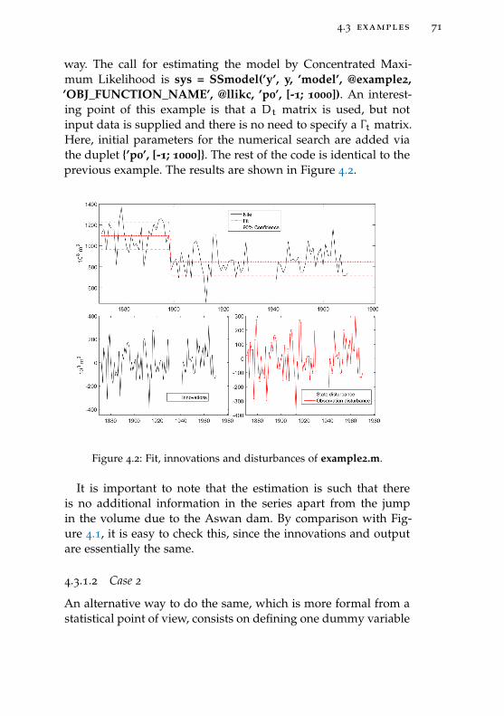
4.3 examples 71
way. The call for estimating the model by Concentrated Maxi-mum Likelihood is sys = SSmodel(’y’, y, ’model’, @example2,’OBJ_FUNCTION_NAME’, @llikc, ’p0’, [-1; 1000]). An interest-ing point of this example is that a Dt matrix is used, but notinput data is supplied and there is no need to specify a Γt matrix.Here, initial parameters for the numerical search are added viathe duplet {’p0’, [-1; 1000]}. The rest of the code is identical to theprevious example. The results are shown in Figure 4.2.
Figure 4.2: Fit, innovations and disturbances of example2.m.
It is important to note that the estimation is such that thereis no additional information in the series apart from the jumpin the volume due to the Aswan dam. By comparison with Fig-ure 4.1, it is easy to check this, since the innovations and outputare essentially the same.
4.3.1.2 Case 2
An alternative way to do the same, which is more formal from astatistical point of view, consists on defining one dummy variable

72 sspace : a toolbox for state space modeling
as a step, taking zeros up to observation 28 and ones afterwards,i.e.: u = [zeros(28, 1); ones(82, 1)]. In this case, the user functionis:
function model = example3(p)
model.T = 1;
model.Gam = [];
model.R = 1;
model.Z = 1;
model.D = p(2);
model.C = 1;
model.Q = 1;
model.H = 10.^p(1);
model.S = 0;
The difference with the previous option is that matrix model.Dis just the second element of the parameter vector p, i.e.: a coef-ficient that will multiply the input dummy variable ut. Now thecall to SSmodel should be:
sys = SSmodel(’y’, y, ’u’, u, ’model’, @example3, ’OBJ’,
@llikc);
Here, the duplet {’u’, u} tells SSpace which is the input variableto use. The estimation of the coefficient measuring the jump isnegative and significant.
4.3.1.3 Case 3
A final case, still worth mentioning, consists of including thedummy input variable into the user function as an additionalinput argument, but now the SS system is considered as a systemwithout inputs:
function model = example4(p, u)
model.T = 1;
model.Gam = [];
model.R = 1;
model.Z = 1;
model.D = p(2)*u;
model.C = 1;
model.Q = 1;
model.H = 10.^p(1);

4.3 examples 73
model.S = 0;
The call now should be:
sys = SSmodel(’y’, y, ’model’, @example4, ’OBJ’, @llikc, ’user_inputs’, {u});
Additional inputs to the user function may be passed on tothe model definition with the help of duplets {’user_inputs’, {u}}.Though it does not make sense in this case, it is worth noting thatthe dependence to the inputs may be modelled by a non-linearfunction, e.g.: just by defining model.D = p(2)*(u(2, :).ˆ (p(3))) orany other specification. This is the main advantages of specifyingmodels by writing a function. More examples may be checked indemo5.
4.3.2 Example 2: Univariate models
In this second example the air-passenger data taken from Boxet al. (2015) is analysed with a number of different univariatepossibilities.
4.3.2.1 Case 1: Basic Structural Model
A Basic Structural Model (BSM) a la Harvey (Harvey, 1989) maybe used with the template SampleBSM (it is also possible touse SampleSS and test the SS form from scratch). In such tem-plate, separate definitions are in place for the trend and the har-monics and input variables, if any. Have a look on the func-tion demo_airpasbsm.m that is one of the cases implementedin demo2.
The part of the template related to the trends is:
m = ;
I = eye(m);
O = zeros(m);
TT = [I I;O I];
ZT = [I O];
RT = [I O; O I];
QT = [];

74 sspace : a toolbox for state space modeling
where the variable m is the number of output variables (1 for uni-variate) and matrices I and O are pre-defined as a unity matrixand a block of zeros. The model is specified directly by the SS
form of the Local Linear Trend (LLT), i.e.:
(α1,t+1
α2,t+1
)=
(1 1
0 1
)(α1,t
α2,t
)+
(1 0
0 1
)(η1,t
η2,t+1
)
A LLT is fully specified by filling in the missing variables in theprevious listing, i.e.: m = 1, and QT = [10.ˆ p(1) 0; 0 10.ˆ p(2)].Other possibilities are implemented by small variations to thisoption, one interesting case is an Integrated Random Walk (IRW)or smooth trend with one single noise by setting RT = [O; I]; QT= 10.ˆ p(1); (Young, Pedregal, and Tych, 1999).
The periodic components (either seasonal or cyclical) in Sam-pleBSM may be coded as either trigonometric or dummy season-ality. For the trigonometric case the empty code in the templateis:
Period = [];
Rho = [];
Qs = repmat( , , );
This portion of the code filled in for a monthly time seriesconverts to:
Period = [12 6 4 3 2.4 2];
Rho = [1 1 1 1 1 1];
Qs = repmat(varmatrix(p(3)), 1, 6);
The argument Period is used to provide the periods for theseasonal and/or cyclical, Rho is the damping factor of each har-monic sinusoid, i.e.: values between zero and one and values ofunity recommended for seasonal harmonics. The variances foreach harmonic are introduced via the Qs matrix (all variancesequal for all the harmonics in the example). If all variances haveto be different the code would be Qs = varmatrix(p(3:8)’). Thefunction varmatrix provides an alternative way of building semipositive definite covariance matrices.
The rest of the template is:

4.3 examples 75
H = varmatrix(p(4));
D = [];
where H is the variance of the observed noise and matrix D isincluded to deal with input variables (none in this case).
Once the BSM model is set up, the code to run is as follows:
load airpas;
y = log(airpas);
sys = SSmodel(’y’, y, ’model’, @demo_airpasbsm);
sys = SSestim(sys);
sys = SSsmooth(sys);
T = sys.a(1, :)’;
I = y-sys.yfit’;
S = y-I-T;
Here the trend, Seasonal and Irregular components are esti-mated by combinations of the estimated states and stored in T, Sand I matrices, respectively.
4.3.2.2 Case 2: ARIMA
The ARIMA model is easily implemented by using the SampleARIMAtemplate used as an example in demo3, checkdemo_airpasarima. Assuming that anARIMA(0, 1, 1)× (0, 1, 1)12is to be estimated, the relevant part of this template is
Sigma = varmatrix(p(3));
Diffy = conv([1 -1], [1 zeros(1, 11) -1])’;
ARpoly = 1;
MApoly = conv([1 p(1)], [1 zeros(1, 11) p(2)])’;
where Diffy is the differencing polynomial in the backshift op-erator B such that Bjyt = yt−j, ARpoly is the AR polynomialand MApoly is the MA polynomial. Check that the differencingorder is the convolution (i.e.: multiplication) of a regular and sea-sonal difference operators, i.e.: ∆∆12 = (1−B)(1−B12). The MApolynomial of the model is (1+ θ1B)(1+Θ1B
12), with p(1)= θ1and p(2)= Θ1. All polynomials are coded as column vectors ofthe corresponding coefficients in ascending order of powers ofthe backshift operator, as it is common in other MATLAB tool-boxes. Though it does not make sense in this example, constraints

76 sspace : a toolbox for state space modeling
among parameters would be very simple to impose, e.g.: if theconstraint θ1 = Θ1 is needed, the MA polynomial may be codedas MApoly = conv([1 p(1)], [1 zeros(1, 11) p(1)])’ .
4.3.2.3 Case 3: Exponential Smoothing
A final illustration for this data is an ETS model a la Hyndman(Hyndman et al., 2008), which template is SampleES, check
demo_airpasES used in demo3. The template filled in for thisexample is:
ModelType = ’AAA12’;
Phi = [];
Alpha = constrain(p(1), [0 2]);
Beta = constrain(p(2), [0 4-2*Alpha]);
AlphaS = constrain(p(3), [0 2]);
D = [];
Sigma = varmatrix(p(4));
The argument ModelType deals with the type of model, thefirst letter stands for the type of level (’N’ for none, ’A’ for ad-ditive and ’D’ for damped with damping factor Phi), the secondletter is the slope type (’N’ for none or ’A’ for additive), and thethird letter stands for the type of seasonal (again either ’N’ or ’A’),and the numbers after those letters is the period of the seasonalcomponent. The rest of the code sets up the α, β and γ parame-ters affecting the level, slope and seasonal components, that aresuppose to be estimated within certain values, see Hyndman et al.(2008). Sigma stands for the variance of the unique noise presentin the model. Input variables may be included by introducing aD matrix as a function of the p vector of parameters.
4.3.3 Example 3: Multivariate Dynamic Harmonic Regression
The models presented so far are univariate and may be easilyextended to multivariate versions. In this example we present anew model that has not yet been used in its multivariate version,namely the multivariate DHR. It is built in the spirit of seeminglyunrelated equations models, i.e.: the relation among the endoge-nous variables is not explicit in the equations, but are modelled

4.3 examples 77
exclusively via non-diagonal covariance matrices of the differentnoises. The specific formulation is given in Equation (4.3).
yt = Trendt + Cyclet + Seasonalt + f(ut) + εtCyclet + Seasonalt =
∑ki=1[Aitcos(ωit) +Bitsin(ωit)]
(4.3)
Obviously yt is multivariate in this case; f(ut) models linearor non-linear relations to inputs; εt is a white noise variable withfull covariance matrix Ht; ωi (i = 1, 2, . . . ,k) are the frequen-cies for the periodic components that typically include the sea-sonal fundamental frequency and all the harmonics down to πbut also may include cyclical frequencies; and Ait and Bit arediagonal matrices of time varying parameters. Usually RandomWalk parameters may suffice, but other options may be preferredin specific applications. In essence the DHR model is effectively amultivariate Fourier analysis in particular frequencies with timevarying parameters. The univariate version of these models esti-mated in the frequency domain where explored by Young, Pedre-gal, and Tych (1999) and Taylor et al. (2007).
These type of models may be easily implemented in SSpacewith the help of the template SampleDHR. This template resem-bles SampleBSM of the previous example, with a user functionthat needs an additional input argument that have to be takeninto account in the SSmodel call, i.e.: the size in time of the sam-ple. In the case of a trivariate model of quarterly data is imple-mented in demo_energydhr used in demo4. A compacted ver-sion of such template is
function model = demo_energydhr(p, N)
% Trend
m = 3;
I = eye(m); O = zeros(m);
TT = [I I;O I];
ZT = [I O];
RT = [I O; O I];
QT = blkdiag(varmatrix(p(1:6)), varmatrix(p(7:12)));
% Seasonal/cyclical DHR components
Periods = repmat([4 2], 3, 1);
Rho = ones(3, 2);
78 sspace : a toolbox for state space modeling
Qs = repmat(varmatrix(p(13:18)), 1, 2);
% Covariance matrix of irregular component (observed noise)
H = varmatrix(p(19:24));
There are a total of 24 unknown parameters, all of them lo-cated at covariances matrices. It is important to note here the useof the varmatrix function, used to convert any set of arbitraryparameters into a semi-positive covariance matrix. Beware that,since covariance matrices are symmetrical, a 3× 3 matrix have 9
elements, but only 6 of them are different. This function allowsalso to impose rank and other constraints to build homogeneousmodels, etc. (see the SSpace documentation). It is also easy tocheck that there are only two harmonics and both are estimatedwith the same covariance matrices, check Qs matrix.
Such model may be run on the energy data of Harvey (1989),with the following code:
load energy
y = log(energy);
p0 = repmat([-2 -2 -2 0 0 0]’, 4, 1);
sys = SSmodel(’y’, y, ’model’, @demo_energydhr, ’p0’, p0, ...
’user_inputs’, length(y));
sys = SSestim(sys);
sys = SSsmooth(sys);
Trend = sys.a(1:3, :)’;
Irregular = y-sys.yfit’;
Seasonal = y-Trend-Irregular;
It is important to initialise the searching algorithm with appro-priate diagonal covariance matrices, this is achieved by the settingof p0 above. The call to SSmodel is done with the required initialparameters and the number of time samples.
Figure 4.3 shows some output of this DHR model.
4.3.4 Example 4: Non-gaussian
The number of van drivers casualties in the UK, see Durbin andKoopman (2012) and Figure 4.4, is a case where a Poisson dis-tribution is justified, because numbers are small and the unitsare integers. Neither the Gaussian assumption is strictly correct

4.3 examples 79
Figure 4.3: Unobserved components of DHR example.
nor the logarithmic transformation manage to produce sensibleresults. The model used is a BSM with a trend, dummy seasonal,irregular and an exogenous effect due to the enforcement of theseat belt law, but the distribution of the observations is a Poisson,see Equation (4.4).
αt+1 = Ttαt + Γt + Rtηt
p(yt | θt) = exp{θ ′tyt − exp(θt) − logyt!}+ bIt(4.4)
In order to set up this model in SSpace we have to create twouser functions, one with the linear model, i.e.: the BSM with adummy seasonal (beware that there is no noise in the observationequation) by using the SampleBSM template and a second one tochange the observation equation into a Poisson model with thehelp of SampleEXP template (other distributions available areBinary, Binomial(n), Negative Binomial and Exponential). Bothfunctions may be checked in demo_van_poisson, used in demo7.The linear model is (function demo_van in file demo_vanl.m):
function model = demo_van(p, H)

80 sspace : a toolbox for state space modeling
% Trend
TT = 1;
ZT = 1;
RT = 1;
QT = varmatrix(p(1));
% Dummy seasonal
Period = 12;
Qs = 0;
% Linear term
D = p(2);
As it may be seen, the model is just a Random Walk trend witha dummy seasonal component and a dummy effect dealing withthe step change due to the seat belt law enforcement.
The second user model is rather simple, it consists of a call tothe linear model above and just telling SSpace that the observa-tions follow a Poisson distribution. This function has the pecu-liarity that necessarily has to have two input arguments, whilethe user may add as many as the model require for its definition:
function model = demo_van_poisson(p, H)
% Call to linear model
model = demo_van(p, H);
% Distribution of observations
model.dist = Poisson;
Then, the following code would produce the analysis for thedata with some artificial missing values in the middle and someat the end to produce the forecasts:
load Van
y = Van(:, 1);
u = Van(:, 2);
y(50:55)= nan;
y = [y; nan(20, 1)];
u = [u; ones(20, 1)];
sys = SSmodel(’y’, y, ’u’, u, ’model’, @demo_van_poisson);
sys = SSestim(sys);
sys = SSvalidate(sys);
sys = SSsmooth(sys);
Figure 4.4 shows the trend with the jump due to the seatbeltlaw effect and twice the standard error confidence bands.
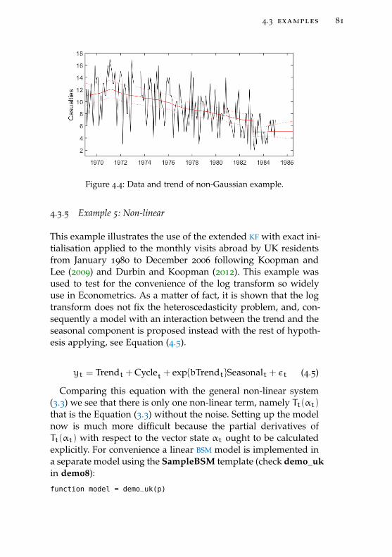
4.3 examples 81
Figure 4.4: Data and trend of non-Gaussian example.
4.3.5 Example 5: Non-linear
This example illustrates the use of the extended KF with exact ini-tialisation applied to the monthly visits abroad by UK residentsfrom January 1980 to December 2006 following Koopman andLee (2009) and Durbin and Koopman (2012). This example wasused to test for the convenience of the log transform so widelyuse in Econometrics. As a matter of fact, it is shown that the logtransform does not fix the heteroscedasticity problem, and, con-sequently a model with an interaction between the trend and theseasonal component is proposed instead with the rest of hypoth-esis applying, see Equation (4.5).
yt = Trendt + Cyclet + exp{bTrendt}Seasonalt + εt (4.5)
Comparing this equation with the general non-linear system(3.3) we see that there is only one non-linear term, namely Tt(αt)that is the Equation (3.3) without the noise. Setting up the modelnow is much more difficult because the partial derivatives ofTt(αt) with respect to the vector state αt ought to be calculatedexplicitly. For convenience a linear BSM model is implemented ina separate model using the SampleBSM template (check demo_ukin demo8):
function model = demo_uk(p)

82 sspace : a toolbox for state space modeling
TT = [1 1;0 1];
ZT = [1 0];
RT = [0; 1];
QT = varmatrix(p(1));
% Trigonommetric seasonal model
Period = [constrain(p(3), [18 800]) 12 6 4 3 2.4 2];
Rho = [constrain(p(4), [0.5 1]) 1 1 1 1 1 1];
Qs = [varmatrix(p(5)) repmat(varmatrix(p(6)), 1, 6)];
% Observed noise variance
H = varmatrix(p(2));
This model has some singularities with respect to previous list-ing in this paper. Firstly, an Integrated Random Walk or smoothtrend is chosen that depends on just one parameter (p(1)). Sec-ondly, a cycle is introduced into the model by adding one ele-ment to all the arguments in the function having to do with theseasonal component. Thirdly, one interesting point is that the pe-riod of such cycle is estimated as a constrained value between 18
and 800 months (one an a half year and 67 years, see the use ofconstrain in Period). Fourthly, the cycle is modulated by a damp-ing factor estimated as a value between 0.5 and 1 (again with thehelp of the constrain function). Finally, separate variance valuesfor the cycle and the seasonal components are estimated.
The non-linear model is now built with the template Sam-pleNL (check model_uknle):
function model = demo_uknle(p, at, ctrl)
model1 = demo_uk(p(1:6));
% Defining linear matrices
if ctrl< 2
model.T = model1.T;
model.Gam = [];
model.R = model1.R;
model.Z = [];
model.D = [];
model.C = 1;
model.Q = model1.Q;
model.H = model1.H;
model.p = p;
model.S = [];
end

4.3 examples 83
% Defining nonlinear matrices in State Equation
if any(ctrl== [2 0])
% Code defining derivative of matrix T(a(t)) (ns x Nsigma)
model.dTa = [];
% Code defining matrix T(a(t)) (ns x Nsigma)
model.Ta = [];
% Code defining matrix R(a(t)) (ns x neps x (1 or n))
model.Ra = [];
% Code defining matrix Q(a(t)) (neps x neps x (1 or n))
model.Qa = [];
end
% Defining nonlinear matrices in Observation Equation
if any(ctrl== [3 0])
b = p(7);
expfun = exp(b*at(1));
S = sum(at(5:2:15));
% Derivative of matrix Z(a(t)) (m x Nsigma)
model.dZa = [1+b*expfun*S 0 1 0 expfun 0 expfun 0 expfun
...
0 expfun 0 expfun 0 expfun];
% Code defining matrix Z(a(t)) (m x Nsigma)
model.Za = at(1)+at(3)+expfun*S;
% Code defining matrix C(a(t)) (Ny x Neps x (1 or n))
model.Ca = [];
% Code defining matrix H(a(t)) (Ny x Ny x (1 or n))
model.Ha = [];
end
This template has three compulsory input arguments, i.e.: theparameter vector p, the current state vector at, and a variable thatcontrols the execution (ctrl). As a first step, the function calls thelinear model demo_uk in order to set up all the matrices in thestate equation. Then the system matrices are redefined in threeblocks, i) linear matrices, ii) non-linear or state-dependent matri-ces in state equation, iii) non-linear or state-dependent matricesin observation equation. Only one definition for each matrix inany of the blocks are permitted, in order to avoid errors. Bewarethat both Zt(αt) (in model.Za) and ∂Zt(αt)
∂αt(model.dZa) have to
be correctly specified.Figure 4.5 shows the estimated components.

84 sspace : a toolbox for state space modeling
Figure 4.5: Series and trend, cycle and raw seasonal and scaled seasonal(exp{bTrendt}Seasonalt) of Non-linear example.
More templates and more demos are available in SSpace thatmay be checked by running carefully the 8 demos included inthe toolbox. Some of the most relevant are linear, non-linear andtime varying regressions (see SampleDLR and demo5), concate-nation of SS systems with the SampleCAT template (a typical casewould be a BSM model with time varying parameters), estimatingparameters of any model by minimizing functions of squared ofseveral-steps-ahead forecast errors (see e.g.: demo2), time aggre-gation problems (see SampleAGG and demo6), and nesting ininputs models (see SampleNEST and demo5).

Part III
A P P L I C AT I O N S


5A S U P P O RT V E C T O R M A C H I N E A P P R O A C HF O R M O D E L S E L E C T I O N
5.1 automatic model selection for forecasting
Companies have traditionally adopted forecasting techniques tosupport decision making on a consistent daily basis, bringingdata from different sources into a common data infrastructure.However, the primal focus was mainly the creation of report-ing tools (Davenport and Harris, 2007). In recent years, the socalled BA introduced a new approach in this domain by lever-aging on the latest progress on both computer science (e.g. datamining algorithms) and hardware technology (e.g. cloud comput-ing, in-memory technology), making possible the integration ofdata sources and business operation on a higher stage of abstrac-tion (Sheikh, 2013).
With the advent of the big data era, the automatic identifica-tion of the appropriate data techniques stands in the middle asa compulsory stage of any big data implementation with predic-tive analytics purposes. Research on model selection and com-bination points out the benefits of such techniques in terms offorecast accuracy and reliability. However, the application of arti-ficial intelligence techniques to such a problem is still scarce.
Forecasting models are of strategic nature given that they gearbusiness decisions ranging from inventory scheduling to strate-gic management (Petropoulos et al., 2014). Focusing on a supplychain context, automatic model selection is a necessity due tothe high number of products whose demand should be forecast(Fildes and Petropoulos, 2015). Forecasting and operational re-
87

88 a support vector machine approach for model selection
search literature has faced the problem with different approaches.A first approach could be aggregate selection, where a singlesource of forecasts is chosen for all the time series (Fildes, 1989),instead of individual selection, where the particular method ap-propriate for each series is selected. However, aggregate selectioncannot distinguish the individual characteristics of each time se-ries (such as trend and/or seasonality) and, in general terms,individual selection outperforms aggregate selection, althoughwith an associated higher complexity level and computationalburden (Fildes and Petropoulos, 2015).
Regarding individual selection, different criteria to choose themost adequate model can be found in the literature. For instance,information criteria like AIC or SBC are typically used (Liang,2014). These information criteria produce a value that representsthe compromise between goodness of fit and the number of pa-rameters. Billah et al. (2006) compare different information cri-teria to select the most appropriate ETS model on simulated dataand a subset of the time series from the M3 competition database,where the AIC slightly outperformed the rest of information crite-ria considered.
The identification of the best forecasting model has also beenaddressed depending on the time series features. Initially, Pegels(1969) presented nine possible ETS methods in graphical form tak-ing into account all combinations of trend and cyclical effects inadditive and multiplicative form. Collopy and Armstrong (1992)developed a rule-based selection procedure model based on a setof 99 rules for selecting and combining between methods basedon 18 time series features. In order to automatize this procedure,Adya et al. (2001) developed and automated heuristics to detectsix features that had previously been judgmentally identified inrule-based selection by means of simple statistics achieving a sim-ilar forecasting accuracy performance. Petropoulos et al. (2014)analysed via regression analysis the main determinants of fore-casting accuracy involving 14 popular forecasting methods (andcombinations of them), seven time series features and the fore-casting horizon as a strategic decision. Wang, Pedrycz, and Liu(2015) propose a rather different approach for long-term forecast-ing based on dynamic time warping of information granules. In-
5.1 automatic model selection for forecasting 89
stead, Yu, Dai, and Tang (2016) focus on finding an empiric de-composition (intrinsic mode functions) to aggregate the individu-ally forecast components later into an ensemble result as the finalprediction. An alternative for selecting among forecasts is the per-formance evaluation of the methods in a hold-out sample (Fildesand Petropoulos, 2015; Poler and Mula, 2011), where forecasts arecomputed for single or multiple origins (cross-validation) usuallyvia a rolling-origin process (Tashman, 2000). Some pragmatic ap-proaches have been used, like forward selection used by Kim,Dekker, and Heij (2017) for determining the order p of an AR
model.Finally, another option is to explore combination procedures
(Clemen, 1989). In fact, Fildes and Petropoulos (2015) concludedthat combination could outperform individual or aggregate selec-tion for non-trended data. Different combination operators (mode,median and mean) to compute neural network ensembles are an-alyzed by Kourentzes, Barrow, and Crone (2014), where the modeis found to provide the most accurate forecasts. Apart from fore-casting models considering time series, it should be noted theautomatic identification algorithms developed for causal mod-els. For instance, marketing analytics models to forecast sales un-der the presence of promotions have been analyzed by Trapero,Kourentzes, and Fildes (2015a). Additionally, models capable ofincorporating data from other companies in a supply chain col-laboration context with information sharing have been exploredby Trapero, Kourentzes, and Fildes (2012).
In addition to traditional time series modeling techniques, Ar-tificial Intelligence algorithms have proved to be quite effectiveas a mean to build higher level methodologies to face big datachallenges in an effective way, gearing upon both traditional andArtificial Intelligence low-level techniques. An initial attempt hasbeen carried out by Turrado, Garcia, and Portela (2012), wheremultiple time series have been classified according to its AutoCorrelation Function (ACF) and Partial Auto Correlation Func-tion (PACF) values to reduce the number of forecasting ARIMA
models to be fitted. However, the forecasting implications of thatprocedure in terms of out-of-sample accuracy was not described.
90 a support vector machine approach for model selection
Despite the abundant literature in model selection, the possi-bility of combining several selection criteria (AIC, SBC) has beenunder-investigated, as well as the benefits of taking advantageof additional pieces of information (ACF and PACF values, fittedparameters, unit root tests, etc.) in an integrated approach thattakes them all into account.
In this chapter, a new model selection approach is proposed. Itcombines different criteria (AIC, SBC, etc.) along with additionalinformation of the time series itself (ACF and PACF values, etc.) aswell as responses and fitted parameters of the alternative mod-els. Given a set of candidate models, instead of considering anyindividual criteria, a SVM is trained at each forecasting origin toselect the best model using all this information.
The effects this approach are explored for the 229 Stock Keep-ing Units (SKU) of a leading household and personal care UKmanufacturer. The data is highly volatile and with small serialcorrelation. The experiment was developed by fitting a set of ETS
and ARIMA models with different levels of complexity. After a fea-ture selection process, only 19 variables were included in the SVM
training dataset as the most relevant. The results show that theproposed approach improves the out-of-sample forecasting accu-racy with respect to single model selection criteria. This method-ology will be particularly interesting for scenarios with highlyvolatile demand, because it allows to change the model when itdoes not fit the data well enough, reducing the risk of misusingmodeling techniques in automatic processing of big datasets.
5.2 methods
5.2.1 Forecasting models
Let yt be the mean-corrected output demand data sampled at aweekly rate, at a white noise sequence (i.e. serially uncorrelatedwith zero mean and constant variance), θi a set of parameters toestimate and B the backshift operator in the sense that Blyt =
yt−l. Then, taking into account the fact that no seasonality is

5.2 methods 91
present in the data, the forecasting models considered are thefollowing:
M1 : yt = at
M2 : yt = (1+ θ1B+ θ2B2)at
M3 (ETS): (1−B)yt = (1+ θ1B)at
M4 : (1−B)yt = (1+ θ1B+ θ2B2)at
Mean : Mean of forecasts M1 to M4
Median : Median of forecasts M1 to M4
(5.1)
Model M1 is white noise, model M2 is a MA(2), model M3 isan IMA(1,1) that is actually treated as a Simple ETS model or aETS(A,N,N) in Hyndman et al. (2008) nomenclature (where E, T,S, A and N stand for Error, Trend, Seasonal, Additive and None,respectively), M4 is an IMA(1,2), and Mean and Median are com-bination methods. In essence, two stationary, three non-stationarymodels and two combinations of models are considered.
It is important to note that some models are nested versionsof others. For example, model M1 is a parametrically efficientversion of the rest of models if θ1 = 0 and θ2 = 0 in modelM2, θ1 = −1 in M3, or θ1 = −1 and θ2 = 0 in M4. Similarly,ETS model M3 is a particular version of M4 with θ2 = 0. Finally,models M2 and M4 are not nested with any other models becauseof the difference operator.
These sort of constraints have been taken into account in theestimation procedure, since when approximate constraints arefound the models preferred are the most parsimonious ones. Thisis particularly important when dealing with estimated roots closeto unity. Specifically, when θ1 < −0.992 in model M3, the modelis switched to M1 for forecasting purposes. Similarly, if any rootin the MA polynomial of model M4 is smaller than −0.992 themodel is switched to a MA(1), that is not any of the models con-sidered above. No unit roots where detected when estimatingmodel M2.
For the 229 SKU time series considered, at least one of the mod-els M1 to M4 above is correct in statistical terms, in the sense thatone of them filters out all the serial correlation present in the data.
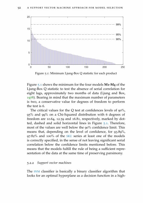
92 a support vector machine approach for model selection
0 50 100 150 200 250
0
5
10
15
20
99%
95%
90%
Figure 5.1: Minimum Ljung-Box Q statistic for each product
Figure 5.1 shows the minimum for the four models M1-M4 of theLjung-Box Q statistic to test the absence of serial correlation foreight lags, approximately two months of data (Ljung and Box,1978). Bearing in mind that the maximum number of parametersis two, a conservative value for degrees of freedom to performthe test is 6.
The critical values for the Q test at confidences levels of 90%,95% and 99% on a Chi-Squared distribution with 6 degrees offreedom are 10.64, 12.59 and 16.81, respectively, marked by dot-ted, dashed and solid horizontal lines in Figure 5.1. Therefore,most of the values are well below the 90% confidence limit. Thismeans that, depending on the level of confidence, for 93.89%,97.82% and 100% of the SKU series at least one of the modelsis correctly specified, in the sense of not leaving significant serialcorrelation below the confidence limits mentioned before. Thismeans that the models fulfill the rule of being a sufficient repre-sentation of the data at the same time of preserving parsimony.
5.2.2 Support vector machines
The SVM classifier is basically a binary classifier algorithm thatlooks for an optimal hyperplane as a decision function in a high-

5.2 methods 93
dimensional feature space (Shawe-Taylor and Cristianini, 2004).Consider the training data set {xk,yk}, where xk ∈ Rn are thetraining examples and yk ∈ {−1, 1} the class labels. The trainingexamples are firstly mapped into another space, referred to asthe feature space, eventually of a much higher dimension thanRn, via the mapping function Φ. Then a decision function ofthe form f(x) = 〈w,Φ(x)〉+ b in the feature space in computedby maximizing the distance between the set of points Φ(xk) tothe hyperplane parameterized by (w,b) while being consistenton the training set. The class label of x is obtained by consid-ering the sign of f(x). In the non-separable case, the misclassi-fied examples are quadratically penalized scaling by a constant C,the cost parameter, and the optimization problem takes the form
minw,ξ
1
2‖w‖2 +C
m∑k=1
ξ2k under the constraint ykf(xk) > 1− ξ2k, ∀k.
Using Lagrangian theory, the optimal vector w is known to havethe form w =
∑mk=1 α
∗kykΦ(xk) where α∗k is the solution of the
following quadratic optimization problem:
maxαW(α) =
m∑k=1
αk−1
2
m∑k,l
αkαlykyl
(K(xk, xl) +
1
Cδk,l
)(5.2)
subject to∑mK=1 ykαk = 0 and αk > 0,∀k, where δk,l is the
Kronecker symbol and K(xk, xl) = 〈Φ(xk),Φ(xl)〉 is the Kernelmatrix of the training examples. The extension for the case ofmulticlass-classification with j levels, j > 2, could be done bythe “one-against-one” approach in which j(j− 1)/2 binary classi-fiers are trained; then the appropriate class is found by a votingscheme (Meyer et al., 2015).
The function K is also known as the kernel function, whichcomputes inner products in the feature space directly from theinputs x. It is supposed to capture the appropriate similarity mea-sure between the arguments, while being computationally muchless expensive than explicitly computing the mapping Φ and in-ner product. Although the design of kernel functions is a very ac-tive research area, there are some popular kernels that have beentested in a variety of domains and applications with good results.The polynomial kernel is defined as K(x, z) = p(〈x, z〉) where p(·) is

94 a support vector machine approach for model selection
any polynomial with positive coefficients. In many cases it alsorefers to the special case Kd(x, z) = (〈x, z〉 + R)d where R andd are parameters. Gaussian kernels (also known as Radial BasisFunctions kernels) are the most widely used kernels and havebeen studied in many different applications. It is defined by
K(x, z) = exp(−‖x− z‖2
2σ2
)(5.3)
where σ is a parameter that controls the flexibility of the kernel.In this study gaussian kernels are extensively used, and the pa-rameter σ is estimated via cross-validation as explained in Section§5.2.3.
Though it was extended to regression problems since its earlydays (Müller et al., 1997), SVM were originally designed as a clas-sification algorithm (Cortes and Vapnik, 1995) and have been ex-tensively exploited in a huge variety of classification contexts, e.g.hand-written digit recognition, genomic DNA (Furey et al., 2000),text classification (Joachims, 2002), sentiment analysis (Pang, Lee,and Vaithyanathan, 2002). But surprisingly SVM have not been ap-plied to the problem of model selection in the context of multipleforecasting models. The approach in this chapter constitutes ancontribution in the area of possible applications of SVM in thisscenario.
5.2.3 Feature selection and extraction
Reliable results in SVM and other data driven modeling techniquesare considerable conditioned to the quality of the data availablefor training. Apart from the correctness of the data itself, there aresome other aspects regarding the dimensionality of the dataset.In fact, it is well known that as the number of variables increases,the amount of data required to provide a reliable analysis growsexponentially (Hira and Gillies, 2015). Many feature selection (re-moving variables that are irrelevant) and feature extraction (ap-plying some transformations to the existing variables to get a newone) techniques have been discussed to reduce the dimensional-ity of the data (Kira and Rendell, 1992), to say nothing about

5.2 methods 95
some other approaches based on linear transformation and co-variance analysis like principal component analysis and lineardiscriminant analysis (Cao et al., 2003; Duin and Loog, 2004). Forthe experiments carried out in this work, the initial dataset con-tained 14885 records (65 origins and 229 products), and 39 fea-tures including SBC and Q statistics, ACF and PACF, fitted param-eters for each model (if any), gaussianity and heterokedasticitytests over residuals, unit tests, relative differences and ranking ofthe alternative models. After a process of feature selection andextraction via cross-validation, the number of variables was re-duced to 19 resulting in a matrix W of dimension 14, 885 × 19.The final features are:
• Four (4) last SKU values available at time t.
• Relative (6) differences among the predictions provided bythe alternative forecasting methods (M1 to M4).
• Four (4) predictions provided by the alternative forecastingmethods (M1 to M4).
• Parameters (5) used by the forecasting methods.
The vector of labels Li is formed as a categorical variable indi-cating the model with lower forecasting error at horizons t+ i for1 6 i 6 4. For horizons t+ 2, t+ 3 and t+ 4 the model with lowerforecasting error is selected as the one that minimizes the totalsum of squared errors in all the spanned weeks t+ 1, · · · , t+ i.
For each week k, with 4 < k < 65, a SVM with a radial basisfunction kernel is trained using the training set Wtrain and thecorresponding vector of labels Li for each forecasting horizon.Wtrain is form as a partition of matrix W including up to fourweeks of history (h = 4), i.e., gathering records for weeks k− 4to k− 1. Similar considerations were done in shaping vector Li.Different values for h were also empirically tested, resulting inh = 4 as the optimal for the current dataset. For optimizing theσ and cost parameters a 5-fold cross-validation was performed.

96 a support vector machine approach for model selection
5.3 case study
The evaluation of the models proposed is carried out on a set of229 demand series from a leading household and personal careUK manufacturer. For each product, there are 173 weekly salesobservations, from which 101 observations are used as in-sampleand the rest are reserved for out-of-sample evaluation. Therefore,a set of 69 forecast rounds of 4 weeks ahead were carried out foreach product. Figure 5.2 shows some examples of the time seriesin the dataset, where the shaded area shows the out-of-sampleperiod. Neither seasonality is visible in the sample SKUs by eyeinspection, nor any strong correlation pattern.
A rolling forecasting experiment is carried out by expandingthe in-sample span one week at a time. All forecasting modelsare fitted in the in-sample partition using the available data upto time T with 101 6 T 6 169, and tested in the out-of-samplepartition using observations T + 1, · · · , T + 4. The out-of-sampleforecasting errors are therefore calculated for the four forecastinghorizons on each of the 229 products. We measure the forecast er-ror using scaled Mean Squared Error (sMSE) and scaled MedianSquared Error (sMdSE) that come from computing the scaled Er-ror (sE) and scaled Squared Error (sSE) of the lead time forecastaccording to the following formulae:
sET+l =
∑lj=1 zT+j −
∑lj=1 zT+j
1T
∑Ti=1 zi
, (5.4)
sSET+l =(∑lj=1 zT+j −
∑lj=1 zT+j)
2
1T
∑Ti=1 zi
, (5.5)
where the denominator is the mean of the time series, zT+j standsfor the forecast at time T + j and l = 1, 2, 3, 4. Using these metricshas the advantage of allowing zero values at some periods of theseries, and makes the results scale independent and therefore wecan summarize them across products and forecasting horizons.Scaled absolute errors were also calculated in addition to squared

5.3 case study 97
0 50 100 150
010
2030
Week
SK
U
In−sample Out−of−sample
0 50 100 150
040
8012
0
Week
SK
U
In−sample Out−of−sample
0 50 100 150
050
150
Week
SK
U
In−sample Out−of−sample
0 50 100 150
020
4060
80
Week
SK
U
In−sample Out−of−sample
Figure 5.2: Example of some SKU from the dataset
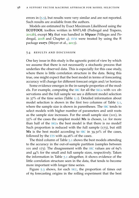
98 a support vector machine approach for model selection
errors in (5.5), but results were very similar and are not reported.Such results are available from the authors.
Models are estimated by Exact Maximum Likelihood using theECOTOOL toolbox written in MATLAB (Pedregal and Trapero,2012b), except M3 that was handled in SSpace (Villegas and Pe-dregal, 2018 and Chapter 4). SVM were treated by using the Rpackage e1071 (Meyer et al., 2015).
5.4 results and discussion
One key issue in this study is the agnostic point of view by whichwe assume that there is not necessarily a stochastic process thatunderlies the observed data. This is especially for this case study,where there is little correlation structure in the data. Being thistrue, one might expect that the best model in terms of forecastingaccuracy will change for different forecast origin and/or horizon.
Some evidence emerges in the in-sample properties of the mod-els. For example, computing the SBC for all the SKUs with 101 ob-servations and the full sample we see a different model selectionin 37% of the time series (Table 5.1). Detailed information aboutmodel selection is shown in the first two columns of Table 5.1,where the sample size is shown in parentheses. The SBC tends toselect models with higher number of parameters and unit rootsas the sample size increases. For the small sample size (101), in55% of the cases the simplest model M1 is chosen, i.e. for morethan half of the SKUs the best model is that there is no model!Such proportion is reduced with the full sample (173), but stillM1 is the best model according to SBC in 39.30% of the cases,followed by the ETS with 29.26% of the cases.
The third column of Table 5.1 shows the best models attendingto the accuracy in the out-of-sample partition (samples between101 and 173). The disagreement with the SBC values are of 69%and 44% for the small and full sample sizes, respectively. Takenthe information in Table 5.1 altogether, it shows evidence of thelittle correlation structure seen in the data, that tends to becomemore important with longer time series.
Figure 5.3 shows, for each SKU, the proportion of times outof 69 forecasting origins in the rolling experiment that the best
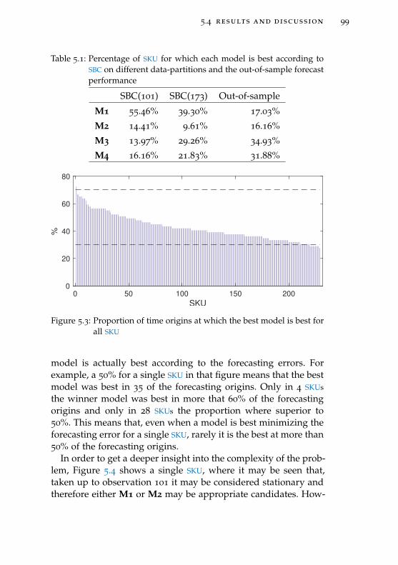
5.4 results and discussion 99
Table 5.1: Percentage of SKU for which each model is best according toSBC on different data-partitions and the out-of-sample forecastperformance
SBC(101) SBC(173) Out-of-sample
M1 55.46% 39.30% 17.03%
M2 14.41% 9.61% 16.16%
M3 13.97% 29.26% 34.93%
M4 16.16% 21.83% 31.88%
0 50 100 150 200
SKU
0
20
40
60
80
%
Figure 5.3: Proportion of time origins at which the best model is best forall SKU
model is actually best according to the forecasting errors. Forexample, a 50% for a single SKU in that figure means that the bestmodel was best in 35 of the forecasting origins. Only in 4 SKUs
the winner model was best in more that 60% of the forecastingorigins and only in 28 SKUs the proportion where superior to50%. This means that, even when a model is best minimizing theforecasting error for a single SKU, rarely it is the best at more than50% of the forecasting origins.
In order to get a deeper insight into the complexity of the prob-lem, Figure 5.4 shows a single SKU, where it may be seen that,taken up to observation 101 it may be considered stationary andtherefore either M1 or M2 may be appropriate candidates. How-
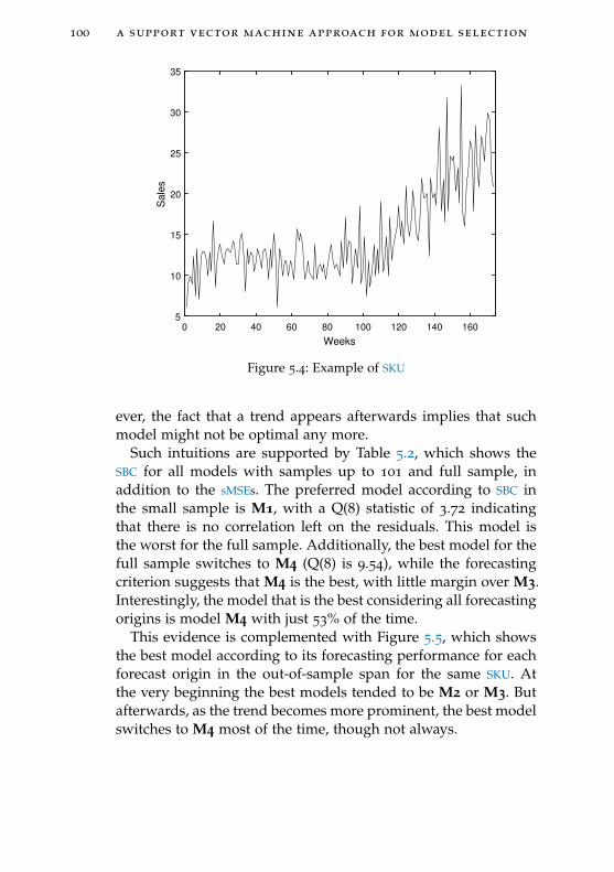
100 a support vector machine approach for model selection
0 20 40 60 80 100 120 140 160
Weeks
5
10
15
20
25
30
35
Sa
les
Figure 5.4: Example of SKU
ever, the fact that a trend appears afterwards implies that suchmodel might not be optimal any more.
Such intuitions are supported by Table 5.2, which shows theSBC for all models with samples up to 101 and full sample, inaddition to the sMSEs. The preferred model according to SBC inthe small sample is M1, with a Q(8) statistic of 3.72 indicatingthat there is no correlation left on the residuals. This model isthe worst for the full sample. Additionally, the best model for thefull sample switches to M4 (Q(8) is 9.54), while the forecastingcriterion suggests that M4 is the best, with little margin over M3.Interestingly, the model that is the best considering all forecastingorigins is model M4 with just 53% of the time.
This evidence is complemented with Figure 5.5, which showsthe best model according to its forecasting performance for eachforecast origin in the out-of-sample span for the same SKU. Atthe very beginning the best models tended to be M2 or M3. Butafterwards, as the trend becomes more prominent, the best modelswitches to M4 most of the time, though not always.

5.4 results and discussion 101
100 110 120 130 140 150 160 170
Weeks
2
3
4
Be
st
mo
de
l M
#
Figure 5.5: Best model for each out-of-sample forecast origin for SKU inFigure 5.4
Table 5.2: SBC for all models in two different data-partitions and sMSE forout-of-sample for SKU in Figure 5.4
SBC(101) SBC(173) sMSE
M1 1.52 3.31 0.053
M2 1.61 2.89 0.038
M3 1.59 2.26 0.013
M4 1.64 2.19 0.012

102 a support vector machine approach for model selection
The previous evidence shows that there is not best model out-performing the rest for all SKUs, all forecasting origins and allforecasting horizons. Moreover, even for a single SKU there is notconsistent best model along time. At this point the SVM-basedensemble approach is introduced in order to test the hypothe-sis that there is some pattern that would allow to improve theforecast accuracy over all models and possible combinations ofthem. In this sense, the proposed approach might be considereda sophisticated combination method in itself.
Table 5.3 shows the scaled mean (median) squared errors for allforecasting models and methods, including a Naïve model (eachforecast is simply equal to the last observed value) that serves asa benchmark. The last row corresponds to the errors generated byselecting the best possible model for every forecasting-step out ofthe models set considered.
Several facts emerge from Table 5.3. Firstly, taken as a whole,all models outperform the Naïve by a wide margin, implying thatall models capture, at least at some part of the experiment, thecorrelation structure of the data. Secondly, for individual modelsM1 to M4 the best is consistently the ETS M3 model, with an ad-vantage that grows with the forecasting horizon. Thirdly, combi-nations of methods (mean and median) do not manage to outper-form the ETS and both provide virtually the same results. Finally,and most importantly, the SVM-based approach is the overall bestfor all forecasting horizons with errors that fall between the M3and the minimum possible forecasting error (that would resultfrom selecting always the model with minimum error). Oncemore, the advantages of the proposed method are appreciatedmore clearly for higher forecast horizons.
Table 5.4 shows the bias considering the sEt measurementsfrom Equation 5.4. All biases are small, bearing in mind that thehighest bias in the table is 0.124 and the normalization imposedon the data implies a mean of 1. Conclusions about bias are quitedifferent depending on whether we rely on sE or scaled MedianError (sMdE), but due to the robustness of the median it is safer touse the sMdE values in parenthesis. In essence, the bias replicateswhat was seen in squared errors, i.e. the models with the smallestsquared errors are at the same time the models with the smallest

5.4 results and discussion 103
Table 5.3: Forecast accuracy for out-of-sample sets in sMSE (sMdSE).
Out t+1 Out t+2 Out t+3 Out t+4
Naïve 0.184 0.558 1.114 1.856
(0.041) (0.128) (0.266) (0.437)
M1 0.115 0.278 0.486 0.743
(0.032) (0.075) (0.134) (0.195)
M2 0.109 0.255 0.447 0.689
(0.030) (0.072) (0.130) (0.192)
M3 0.100 0.221 0.363 0.533
(0.026) (0.054) (0.087) (0.123)
M4 0.102 0.230 0.380 0.555
(0.027) (0.059) (0.096) (0.139)
mean 0.101 0.226 0.374 0.549
(0.027) (0.060) (0.101) (0.150)
median 0.101 0.225 0.373 0.549
(0.027) (0.059) (0.101) (0.150)
SVM-based 0.099 0.212 0.334 0.471
(0.026) (0.052) (0.081) (0.110)
Baseline 0.071 0.149 0.234 0.327
(0.011) (0.022) (0.034) (0.049)

104 a support vector machine approach for model selection
Table 5.4: Forecast bias multiplied by 102 for out-of-sample sets in sE
(sMdE).
Out t+1 Out t+2 Out t+3 Out t+4
M1 0.317 0.785 0.903 1.024
(-4.690) (-5.252) (-6.199) (-7.295)
M2 -0.242 -0.345 -0.208 -0.068
(-4.598) (-5.185) (-5.336) (-7.914)
M3 -1.259 -2.367 -3.826 -5.282
(-4.006) (-3.909) (-3.101) (-3.627)
M4 -2.041 -4.230 -6.769 -9.307
(-4.508) (-4.693) (-5.004) (-5.672)
mean -0.807 -1.539 -2.475 -3.408
(-4.474) (-4.853) (-5.546) (-6.134)
median -0.832 -1.715 -2.669 -3.614
(-4.589) (-5.068) (-5.094) (-6.241)
SVM-based 0.309 0.155 -0.610 -2.365
(-3.013) (-2.403) (-1.310) (-2.652)
Baseline 0.002 -0.713 -1.961 -3.193
(-1.246) (-1.123) (-0.939) (-1.635)

5.4 results and discussion 105
bias. The best is the SVM-based method, followed by the ETS (M3),then model M4 and combinations of models.
The SVM-based approach is allowed to select among the differ-ent forecasting models at each forecast origin, and therefore, it israther more flexible to adapt to stochastic or structural changes inthe SKUs. This fact explains why SVM-based criterion outperformsall the considered alternatives in forecast accuracy.


6A U T O M AT I C A P P R O A C H F O R U C M O D E LS E L E C T I O N
6.1 problem overview
The present chapter complements the previous one in the sensethat it deals with the topic of automatic model selection, but froma completely different point of view. Indeed, the previous chapterexplored a novel individual approach, by which the best forecast-ing option is selected at each single step among a menu of possi-bilities. However, this chapter would adopt an aggregate approach,meaning that the focus is now on selecting one single method toforecast all the time series available in a database (Fildes, 1989).The aim is to explore whether automatically identified UC modelscompare favorably with other, better known methods, especiallyETS and ARIMA.
ETS continues to be the most used modeling technique in busi-ness and industry, at least in areas ranging from inventory man-agement and scheduling to planning. Its endurance over time isstriking, especially as it started as an ad-hoc method for smooth-ing and forecasting time series in the 1950’s (Gardner, 1985, 2006).The main reasons for its longevity are probably its good perfor-mance in general applications and its intuitive appeal, as it is easyto understand and to communicate to company managers. Thefact that they were not grounded in statistics has fueled a rootand branch revision in the last 20 years that has dramaticallychanged the view held of ETS techniques, including automaticidentification tools and software (Hyndman et al., 2008; Hynd-man and Khandakar, 2008).
107
108 automatic approach for uc model selection
The second most widespread methodology after ETS is, to allappearances, ARIMA. More recent than ETS, ARIMA models haveexpanded since the 1970’s after the publication of the influentialbook by Box and Jenkins (Box et al., 2015). Different automaticidentification procedures have been proposed (Gómez and Mar-avall, 2001; Hyndman and Khandakar, 2008), with TRAMO (inconjunction with SEATS) probably being the most used ARIMA
automatic identification procedure in statistical agencies all overthe world.
At the same time, the academic literature on the topic hasevolved much more than its practical implementation in businessand industry, which for the most part remain staunch advocatesof ETS and ARIMA. Numerous papers can be found that add newdimensions to the problem, such as judgmental forecasting, mod-eling the bullwhip effect, intermittent demands, promotions, etc.(Croston, 1972; Syntetos and Boylan, 2001; Trapero, Kourentzes,and Fildes, 2015b; Trapero and Pedregal, 2016; Trapero et al.,2013). However, many other papers focus on comparing othertechniques, such as Artificial Neural Networks, models with in-puts, etc. Fildes et al. (2008), Syntetos, Boylan, and Disney (2009),and Syntetos et al. (2016) provide comprehensive surveys.
Despite the wealth of literature on the topic, there is a fam-ily of models that has been systematically overlooked, namelystructural UC models (Durbin and Koopman, 2012; Harvey, 1989;Young, Pedregal, and Tych, 1999).
UC models aim at decomposing a vector of time series intomeaningful components explicitly, namely trend, seasonal, andirregular. Other components may be considered as well, typicallycycles and components relating the output variables to inputsmodeled as linear regressions, transfer functions or non-linear re-lationships. A general representation was given in equation (4.3)and is reproduced here for convenience, with small change, con-sisting in the irregular component It, that in this chapter may becolored.
yt = Trendt + Cyclet + Seasonalt + f(ut) + It (6.1)
6.1 problem overview 109
Many consider Harrison and Stevens (1976) as a seminal workin UC methods, though there have been some big milestones inthe posterior development, being Harvey (1989) one of the mostimportant. Since then, UC models has been an ever growing re-search area.
The main problem with models like (6.1) is finding ways to as-sure feasible extraction of meaningful components. This is achievedby imposing identification constraints. Depending on the waythis is done, UC methods may be classified into two big groups:i) reduced-form methods (Gómez and Maravall, 2001) that start-ing on a reduced ARIMA model find the structural componentscompatible with it, and ii) structural methods (Harvey, 1989) thatspecify models for the structural components directly (the re-duced form may be estimated, if required).
Despite the growth of UC methods in many research areas, ithas not been tested in a supply chain environment for at leastfour reasons. First, UC have been developed in academic environ-ments, with no strategy for their dissemination among practition-ers for their everyday use in business and industry. They havebeen applied to a certain degree in state agencies with modestsuccess in terms of dissemination, due to the overwhelming useof X-12-ARIMA and its predecessors, TRAMO and SEATS. Sec-ond, the widely-held but not-scientifically-tested feeling that UC
models do not really have anything relevant to add to ETS meth-ods has deterred its use in practice (UC “bear many similaritiesto exponential smoothing methods, but have multiple sources ofrandom error. In particular, the BSM is similar to Holt-Winters’method for seasonal data and includes level, trend and seasonalcomponents”, see De Gooijer and Hyndman, 2006). Third, UC
models are usually identified by hand, with automatic identifica-tion being very rare. Finally, software is scarcer and sparser thanstandard packages, some genuine alternatives are e.g., STAMP(Koopman et al., 2009), SSfpack (Koopman, Shephard, and Doornik,2008), SSpace (Villegas and Pedregal, 2018 and Chapter 4).
A good demonstration of the lack of use of UC models com-pared to other methods is that they are not included in manyforecasting competitions and studies of forecasting comparisonsin supply chain contexts. The list is too long to quote here, but

110 automatic approach for uc model selection
some examples are Athanasopoulos et al. (2011), Fildes et al.(2008), Makridakis and Hibon (2000a), Syntetos, Boylan, and Dis-ney (2009), and Syntetos et al. (2016). Some of the procedures inthese references do in fact involve a comprehensive search amongmany possibilities as the application of an expert system, butnone includes UC models.
The alleged similarities between UC and ETS deserve a spe-cial comment. There is no doubt that there are similarities, butsuch a broad statement requires a more rigorous evaluation. Inshort, ETS and UC share common ground in the same way that ETS
and ARIMA, or UC and ARIMA, do. The key point is that UC havetheir own avenues of development, with some areas that clearlyoverlap with ETS and ARIMA, while other areas are quite distinct,which is what makes each of the techniques useful in its ownway.
The main advantages of ETS methods according to Hyndmanet al. (2008) and Hyndman and Khandakar (2008) are, for exam-ple, their intuitive appeal, their ability to handle multiplicative-additive mixed models in a very efficient way, the use of a linearinnovation state space model and the development of an auto-matic identification procedure for different combinations of trendmodels, seasonals and noises.
Without taking anything away from ETS, UC models are muchmore flexible in several ways, and it is hard to imagine any ETS
modification that cannot be implemented in a UC context (in-deed, some improvements in UC may also be implemented inETS). For example, mixed multiplicative-additive models couldbe replicated as a UC model with the aid of a non linear statespace model and the Extended KF and Smoother, although at thecost of a higher computational burden. A further example is thatthe single source of noise assumed in ETS is in fact an unneces-sary constraint, at least seen from the point of view of UC. Whythe noise of trends and seasonal components ought to be thesame? The point is especially puzzling, because well-known ef-ficient solutions are available for multiple noise models (Durbinand Koopman, 2012). Nevertheless, the single noise structure isperfectly implementable in a UC model, if such an option is con-sidered absolutely essential.

6.1 problem overview 111
UC also have further advantages. First, there are no limitationson the type of trends (or ‘levels’) one may choose for a model.Although most typical trends are Local Level (or Random Walk)or a LLT, other types are Integrated Random Walk, Double In-tegrated Random Walk, Smoothed Trend or Smoothed RandomWalk (Harvey, 1989; Young, Pedregal, and Tych, 1999). Second,the same is true of the seasonal component: the simplest is adummy seasonal, but trigonometric or DHR with common or dif-ferent hyper-parameters and noises for the harmonics involvedcan also be implemented. Spectral tools are very useful in thisrespect (Young, Pedregal, and Tych, 1999). Modulated seasonal-ity may be very interesting in certain applications (Pedregal andYoung, 2006). Third, several cycles may be introduced and areoften introduced in applied work as trigonometric or DHR com-ponents. Once again, spectral analysis is very valuable in thiscase. The mean periods of the cycles may be estimated jointlywith other parameters if required (Harvey, 1989). Fourth, extend-ing univariate UC to include inputs is straightforward - a topicthat seems very relevant to model outliers and the effect of salespromotions. These can be entered as linear regression terms withconstant or time varying parameters, transfer functions, or evennon linear functions (Harvey, 1989). Finally, multivariate UC mod-els are also available (Durbin and Koopman, 2012).
In order to contribute to the dissemination of UC models to awider audience, in this chapter a general Automatic ForecastingSupport System is built for the 166 products of a food franchisechain sold in more than 100 stores throughout Spain. Althoughdeveloped on this dataset, the system can be applied as is toother datasets, and consists of fitting a set of models built onsome traditional models such as ETS and ARIMA models with dif-ferent levels of complexity. The novelty of the system, however,is that UC are also included as a valuable alternative option. Allthe models in the system are cast in a common SS framework thatis new in two ways. First, as far as the authors know, this is thefirst occasion on which UC models have been used in a supplychain forecasting context. Second, it is the first time that auto-matic identification of UC has been proposed. This chapter showsthat UC are in fact a very powerful choice for forecasting and that

112 automatic approach for uc model selection
they may indeed be identified automatically, which is a standardfeature of many other competitors nowadays.
6.2 forecasting methods
All the univariate models shown in this section are suitable forthe general linear and Gaussian SS framework, whose generalformulation is given by equation (3.1).
6.2.1 Benchmarks
Two methods usually found in the literature are tested here asbase benchmarks to be improved on: the seasonal Naïve and AR.The seasonal Naïve produces forecasts that are simple projectionsof the last seasonal span into the future.
AR models seek to capture the correlation structure of a time se-ries by regressing a stationary output variable on its past values.Because of the stationarity condition, regular and seasonal differ-ence operators are usually applied to the initial non-stationarydata (Box et al., 2015). A general AR(p) model is:
zt = (1−B)d(1−B7)Dyt
zt =∑pi=1φizt−i + et =
1(1−φ1B−···−φpBp)
et(6.2)
where et is a white noise sequence (i.e., serially uncorrelated withzero mean and constant variance); B stands for the backshift op-erator so Blyt = yt−l; (1−B) is the difference operator; (1−B7)is the seasonal difference operator (the power of B is 7 in thiscase, as the data is daily with a weekly seasonal); d and D arethe regular and seasonal integer difference orders necessary toinduce stationarity; φi are a set of parameters to estimate; andyt is the stationary series, obtained from differencing the orig-inal, non-stationary data, yt. A constant should be included inthe model if the mean of the differenced series zt is not zero.

6.2 forecasting methods 113
6.2.2 Autoregressive Integrated Moving Avarage model
This is an extension of the previous model to include multiplica-tive polynomials both in autoregressive and moving average terms,popularized by Box et al. (2015). The formulation of an ARIMA(p,d,q)×(P,D,Q)7 model for the stationary time series yt is:
zt =(1+ θ1B+ ... + θqBq)(1+φ1B+ ... +φpBp)
(1+Θ1B7 + ... +ΘQB7Q)
(1+Φ1B7 + ... +ΦPB7P)et (6.3)
where new parameters appear, namely θi(i = 1, 2, . . . ,q), Θj(j =1, 2, . . . ,Q) and Φk(k = 1, 2, . . . ,P).
In this chapter, the general model (6.3) is cast into a SS frame-work and estimated by Exact Maximum Likelihood with the helpof the SSpace toolbox, see Chapter 4 and Villegas and Pedregal(2018).
6.2.3 ExponenTial smoothing
The main principle in exponential smoothing is that forecasts arebuilt as a correction of the last observation by a weighted aver-age of past forecast errors that decay following an exponentialpattern. This pattern is applied to reflect the fact that the mostrecent information is more valuable for forecasting the immedi-ate future than the oldest data. The simplest version is Brown’ssingle exponential smoothing (Brown, 1959), shown in equation(6.4), where a hat on a variable stands for a forecast of the vari-able.
yt+1 = yt +α(yt − yt) (6.4)

114 automatic approach for uc model selection
This simple method may be extended in many different ways,one common is the well-known Holt-Winters method with sea-sonality (Winters, 1960), see equations (6.5).
Level : lt = α(yt − St−7) + (1−α)(lt−1 + bt−1)
Slope : bt = β(lt − lt−1) + (1−β)bt−1
Seasonal : St = γ(yt − lt−1 − bt−1) + (1− γ)St−7
Forecast : yt+1 = lt + bt + St−7
(6.5)
ETS techniques have recently been revised in depth and ex-tended in many respects. The main point is that the approach hasbeen set up in a SS formal framework with the possibility of intro-ducing statistical principles in the process of estimation and fore-casting. Other additions include the use of damped trends, mix-ing multiplicative and additive components in one single model,using a SS framework, and even considering multivariate versions.A detailed description of most of these alternatives can be foundin Hyndman et al. (2008).
6.2.4 Unobserved components models
The UC models considered in the case study below is a simplifiedversion of Equation (6.1) in which the cycle and the inputs arenot necessary. The model is (6.6).
yt = Trendt + Seasonalt + It (6.6)
In this structural approach, the key issue is to select appro-priate dynamic models for each of the components involved. Ingeneral terms, trends should have at least one unit root, seasonalcomponents should show up some kind of stochastic sinusoidaldynamic behaviour, and irregular components should be eitherwhite or coloured noise.
The particular models selected for each component steam fromthe long tradition of UC models since the early Harrison andStevens (1976), to Harvey (1989), Young, Pedregal, and Tych (1999)and Durbin and Koopman (2012), among many others.
6.2 forecasting methods 115
Trends are usually taken from the following family, that resem-bles closely the options introduced in an ETS context by Hyndmanet al. (2008):
[Trendt+1T∗t+1
]=
[α 1
0 1
][TrendtT∗t
]+
[ηt
η∗t
](6.7)
where T∗t is referred to as the ‘slope’ of the trend, 0 < α 6 1, ηtand η∗t are independent white noise sequences with variances σ2ηand σ2η∗ , respectively. This model is called Smoothed Trend andsubsumes the following specific cases: i) Random Walk, by elim-inating the second equation and α = 1; ii) Integrated RandomWalk with α = 1 and σ2η = 0; iii) Smoothed Random Walk withσ2η = 0; and iv) LLT with α = 1, see e.g., Harvey (1989), Tayloret al. (2007) and Durbin and Koopman (2012).
Seasonal components used in this thesis take a stochastic trigono-metric form (Harvey, 1989). The seasonal component is built asthe sum of individual sinusoidal terms for the fundamental pe-riod s and its harmonics. The number of harmonics in general is[s/2] = s/2 for even s numbers, and [s/2] = (s− 1)/2 for odd snumbers. For the daily data with a weekly seasonal of the casestudy below s = 7 and there are three harmonics with periods7/j, j = 1, 2, 3. The seasonal component is then
Seasonalt =3∑j=1
S(j)t
The basic component for the j− th harmonic is the following:
[S(j)t+1
S∗(j)t+1
]=
[cosλj sinλj
−sinλj cosλj
][S(j)t
S∗(j)t
]+
[ψ(j)t
ψ∗(j)t
](6.8)
where λj = 2πj/s is the frequency of each harmonic, S∗(j)t isan additional state necessary for the specification, and ψ(j)
t andψ∗(j)t are independent white noises with common variance σ2j .

116 automatic approach for uc model selection
The so called BSM of Harvey (1989) is composed of the combina-tion of Equation 6.6, a seasonal component with a common noisevariance for the fundamental frequency and all its harmonics,i.e., σ2j = σ2, j = 1, 2, 3, and a white noise irregular component. Itis very important to note that although BSM assumes one singlevariance parameter for all the harmonics, it also assumes differ-ent independent noises for all the harmonics, even for both noiseswithin one harmonic, i.e., ψ(j)
t and ψ∗(j)t for same j. This is rathermore flexible that one single parameter and one single noise forthe seasonal component, as is the usual case in ETS models.
However, this basic specification sometimes leaves some serialcorrelation in the innovations. This problem may be tackled intwo complementary ways, namely, by introducing higher flexibil-ity in the seasonal component by allowing different variances foreach harmonic noise (Young, Pedregal, and Tych, 1999), or/andselecting a coloured noise for the irregular component (Harvey,1989).
Typically coloured noises are included as AR models of loworder. Equation (6.9) shows an example for an AR(2), that maybe easily extended to higher orders.
(It+1
I∗t+1
)=
(φ1 1
φ2 0
)(It
I∗t
)+
(1
0
)εt (6.9)
where I∗t is an additional state with no particular meaning, εt iswhite noise, and φ1 and φ2 are the parameters modulating thedynamics of the AR model.
The model is built by assembling all the parts in a single dy-namic model. As a matter of fact, equation (6.6) is the observationequation of a SS system and the block concatenation of all modelsfor the trend, seasonal and irregular form the transition equation.Block concatenation means stacking all vectors on top of eachother and create diagonal block matrices with all the squaredmatrices.
6.3 automatic model selection 117
6.2.5 Combination of methods
The combination of forecasts has received considerable attentionin the literature with overwhelming evidence that combining fore-casts improves forecasting performance, see e.g., Kourentzes, Bar-row, and Crone (2014) and Makridakis and Hibon (2000b). De-spite many different methods existing for combining forecastingmethods, often the simplest alternatives, such as mean and me-dian, are the optimal choice, see Barrow and Kourentzes (2016)and references therein. Mean and median of ARIMA, ETS and UC
methods are included in this study for the sake of comparison.
6.3 automatic model selection
This section briefly summarizes the specific algorithms for auto-matic model selection for each of the family models consideredin this chapter. All of these follow the general approach of search-ing in a wide model space with a given criterion, SBC in our case,combined in some cases with some data pre-processing, as spec-ified below. The desired result is a parsimonious model, albeitsufficiently complex to be a correct statistical representation ofthe data.
6.3.1 AR and ARIMA
The automatic identification of ARIMA models is carried out intwo steps in a modified version of Hyndman and Khandakar(2008). The first step consists of identifying the regular and sea-sonal integration orders (d and D). In the second step, the modelspace is searched in an intelligent way using SBC.
The way in which the integration orders of time series is han-dled in Hyndman and Khandakar (2008) and in forecast packagein R is by means of formal unit root statistical tests. Applied toour dataset, unit roots formal tests repeatedly produced wrongseasonal integration orders, leading to forecasts that were mis-aligned with the true data. Several more robust alternatives areavailable in the literature: i) some based directly on information
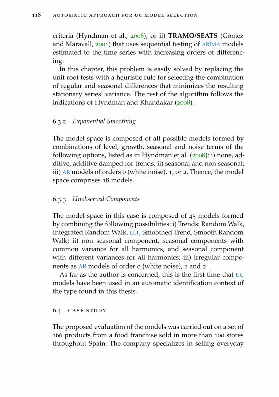
118 automatic approach for uc model selection
criteria (Hyndman et al., 2008), or ii) TRAMO/SEATS (Gómezand Maravall, 2001) that uses sequential testing of ARIMA modelsestimated to the time series with increasing orders of differenc-ing.
In this chapter, this problem is easily solved by replacing theunit root tests with a heuristic rule for selecting the combinationof regular and seasonal differences that minimizes the resultingstationary series’ variance. The rest of the algorithm follows theindications of Hyndman and Khandakar (2008).
6.3.2 Exponential Smoothing
The model space is composed of all possible models formed bycombinations of level, growth, seasonal and noise terms of thefollowing options, listed as in Hyndman et al. (2008): i) none, ad-ditive, additive damped for trends; ii) seasonal and non seasonal;iii) AR models of orders 0 (white noise), 1, or 2. Thence, the modelspace comprises 18 models.
6.3.3 Unobserved Components
The model space in this case is composed of 45 models formedby combining the following possibilities: i) Trends: Random Walk,Integrated Random Walk, LLT, Smoothed Trend, Smooth RandomWalk; ii) non seasonal component, seasonal components withcommon variance for all harmonics, and seasonal componentwith different variances for all harmonics; iii) irregular compo-nents as AR models of order 0 (white noise), 1 and 2.
As far as the author is concerned, this is the first time that UC
models have been used in an automatic identification context ofthe type found in this thesis.
6.4 case study
The proposed evaluation of the models was carried out on a set of166 products from a food franchise sold in more than 100 storesthroughout Spain. The company specializes in selling everyday
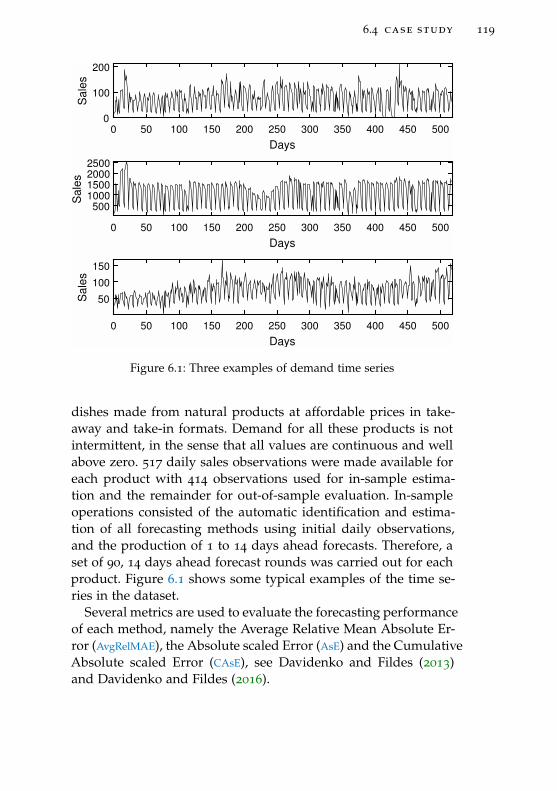
6.4 case study 119
0 50 100 150 200 250 300 350 400 450 500
Days
0
100
200
Sale
s
0 50 100 150 200 250 300 350 400 450 500
Days
5001000150020002500
Sale
s
0 50 100 150 200 250 300 350 400 450 500
Days
50
100
150
Sale
s
Figure 6.1: Three examples of demand time series
dishes made from natural products at affordable prices in take-away and take-in formats. Demand for all these products is notintermittent, in the sense that all values are continuous and wellabove zero. 517 daily sales observations were made available foreach product with 414 observations used for in-sample estima-tion and the remainder for out-of-sample evaluation. In-sampleoperations consisted of the automatic identification and estima-tion of all forecasting methods using initial daily observations,and the production of 1 to 14 days ahead forecasts. Therefore, aset of 90, 14 days ahead forecast rounds was carried out for eachproduct. Figure 6.1 shows some typical examples of the time se-ries in the dataset.
Several metrics are used to evaluate the forecasting performanceof each method, namely the Average Relative Mean Absolute Er-ror (AvgRelMAE), the Absolute scaled Error (AsE) and the CumulativeAbsolute scaled Error (CAsE), see Davidenko and Fildes (2013)and Davidenko and Fildes (2016).

120 automatic approach for uc model selection
0 20 40 60 80 100 120 140 160
Product number
0.2
0.4
0.6
0.8
1
1.2
1.4
CsE
14
Minimum
Maximum
Figure 6.2: Minimum and maximum values of CsE14 for four modelsand each product.
Calling ri =MAEAiMAEBi
the ratio of the Mean Absolute Error (MAE)
of model A over the MAE of benchmark model B for time seriesi, the AvgRelMAE for horizon h and m time series is defined as thegeometric mean of the ri for a chosen h, see Equation 6.10.
AvgRelMAEh = exp
(1
m
m∑i=1
ln ri
)(6.10)
AvgRelMAE shows how the adjustments improve/reduce the MAE
compared to the benchmark (seasonal Naïve in later examples)statistical forecast. Values below 1 means that on average themodel outperforms the benchmark. Values above 1 indicates theopposite.
The AsE with origin T and forecast horizon h (sEh) is definedas
sEh =|zT+h − zT+h|1T
∑Ti=1 zi
(6.11)
The denominator is included to normalize the errors so as tobe able to summarize the results across different products. Re-sults in the case study are robust to replacing the absolute error

6.4 case study 121
with squared errors in equation (6.11) and are available from theauthors upon request. Taking sEh as the basic metrics, the meanand median can be considered valid measures for aggregatedforecast performance across all products.
Finally, the CAsE with origin T and forecast horizons from 1 toh (CsEh) is defined as the cumulative mean of sEh up to horizonh, i.e.,
CsEh =1
h
h∑l=1
|zT+l − zT+l|1T
∑Ti=1 zi
(6.12)
Figure 6.2 shows the maximum and minimum CsE14 values forall models across all individual products, excluding the seasonalNaïve, to avoid distortions. There is considerable variation in theforecastability of each product, since the errors vary wildly. Therelevance of Figure 6.2 is that, although differences in forecasterrors are detected across models and products, all models be-have similarly for the same product in that, when forecast errorsare high, all the models show high errors, and vice versa. Thisensures that the overall forecasting results are not influenced byextreme values or any other sort of anomaly in the data or in theidentification or estimation procedures.
Tables 6.1 and 6.2 show the AvgRelMAE, the median and 75%percentile of sEh for all products, all forecast origins and someselected forecast horizons. Table 6.3 shows the median and 75%percentile for CsEh, and it is complemented in a graphical formby Figure 6.3 excluding the seasonal Naïve model.
Several conclusions may be extracted from this information:
• As expected, forecasting performance worsens with longerhorizons.
• All methods outperform both the seasonal Naïve and AR
benchmarks by a wide margin. Although AR is only consid-ered here as a benchmark, it systematically outperforms theseasonal Naïve.
• UC is the best model for all forecast horizons, followed byARIMA and ETS.

122 automatic approach for uc model selection
0.22
0.24
0.26
0.28
0.3
Me
dia
n
2 4 6 8 10 12 14
Horizon
0.41
0.42
0.43
0.44
0.45
0.46
0.47
75
% p
erc
en
tile
ARIMA
AR
ETS
UC
Mean
Median
Figure 6.3: Median (top panel) and 75% percentile (bottom panel) ofCsEh for all models excluding the seasonal Naïve.
Table 6.1: AvgRelMAE for selected forecasting horizons. Boldface used tohighlight minimum values of each column.
AvgRelMAE 1 2 3 4 7 10 14
AR 0.807 0.854 0.869 0.880 0.890 0.913 0.915
ARIMA 0.740 0.783 0.801 0.814 0.825 0.829 0.839
ETS 0.756 0.802 0.817 0.828 0.836 0.844 0.847
UC 0.730 0.772 0.790 0.801 0.813 0.817 0.824
Mean 0.735 0.778 0.795 0.807 0.820 0.824 0.831
Median 0.733 0.776 0.792 0.804 0.815 0.821 0.828

6.4 case study 123
Table 6.2: Median and 75% percentile of sEh for selected forecasting hori-zons.
Median 1 2 3 4 7 10 14
NAIVE 0.270 0.270 0.269 0.269 0.270 0.279 0.282
AR 0.238 0.252 0.253 0.257 0.261 0.272 0.276
ARIMA 0.216 0.228 0.232 0.235 0.238 0.243 0.249
ETS 0.219 0.234 0.239 0.241 0.241 0.248 0.252
UC 0.211 0.223 0.228 0.230 0.232 0.237 0.243
Mean 0.216 0.227 0.231 0.233 0.239 0.246 0.248
Median 0.215 0.227 0.231 0.233 0.236 0.242 0.246
75% perc. 1 2 3 4 7 10 14
NAIVE 0.573 0.574 0.572 0.574 0.579 0.590 0.592
AR 0.459 0.490 0.503 0.511 0.521 0.549 0.551
ARIMA 0.429 0.458 0.470 0.474 0.485 0.494 0.504
ETS 0.440 0.471 0.479 0.486 0.489 0.506 0.508
UC 0.422 0.443 0.457 0.460 0.469 0.481 0.483
Mean 0.426 0.453 0.464 0.468 0.481 0.490 0.499
Median 0.428 0.452 0.464 0.470 0.479 0.492 0.494

124 automatic approach for uc model selection
Table 6.3: Median and 75% percentile of CsEh for selected forecastinghorizons.
Median 1 2 3 4 7 10 14
NAIVE 0.270 0.314 0.331 0.342 0.355 0.363 0.369
AR 0.238 0.272 0.288 0.298 0.312 0.323 0.328
ARIMA 0.216 0.249 0.265 0.275 0.290 0.296 0.299
ETS 0.219 0.253 0.267 0.279 0.293 0.298 0.302
UC 0.211 0.243 0.260 0.269 0.283 0.290 0.294
Mean 0.213 0.247 0.262 0.272 0.287 0.293 0.297
Median 0.214 0.246 0.261 0.271 0.286 0.292 0.295
75% perc. 1 2 3 4 7 10 14
NAIVE 0.573 0.561 0.551 0.548 0.541 0.537 0.538
AR 0.459 0.461 0.463 0.464 0.467 0.474 0.474
ARIMA 0.429 0.433 0.433 0.431 0.436 0.439 0.439
ETS 0.440 0.445 0.448 0.446 0.442 0.450 0.450
UC 0.422 0.425 0.427 0.425 0.424 0.427 0.430
Mean 0.424 0.427 0.430 0.428 0.429 0.434 0.435
Median 0.422 0.428 0.429 0.427 0.428 0.434 0.435
• Simple forecast combination methods outperform ARIMA
and ETS but do not improve on UC. The performance ofARIMA and ETS is very similar in this case, mainly due tothe absence of important outliers.
• The median of CsEh and sEh (see middle panel of Figure6.3 and Table 6.3) shows that, although UC is a better option,all the models, with the exception of AR and seasonal Naïve(not included in the Figure) offer very similar results. Thismeans that it is hard to find differences in the models withperformance below the median values. However, as the bot-tom panel shows, differences are more apparent when the75% percentile is considered. The advantage of UC modelsis clearer in these cases.
A robustness test checks for the independence of the resultsfrom the software used. Part of the experiment was repeated with
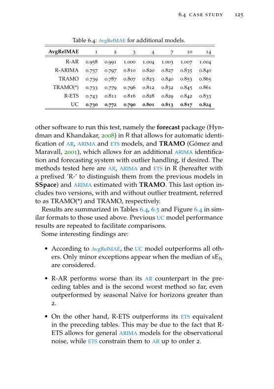
6.4 case study 125
Table 6.4: AvgRelMAE for additional models.
AvgRelMAE 1 2 3 4 7 10 14
R-AR 0.958 0.991 1.000 1.004 1.003 1.007 1.004
R-ARIMA 0.757 0.797 0.810 0.820 0.827 0.835 0.840
TRAMO 0.739 0.787 0.807 0.823 0.840 0.853 0.865
TRAMO(*) 0.733 0.779 0.796 0.812 0.832 0.845 0.861
R-ETS 0.743 0.811 0.816 0.828 0.829 0.842 0.833
UC 0.730 0.772 0.790 0.801 0.813 0.817 0.824
other software to run this test, namely the forecast package (Hyn-dman and Khandakar, 2008) in R that allows for automatic identi-fication of AR, ARIMA and ETS models, and TRAMO (Gómez andMaravall, 2001), which allows for an additional ARIMA identifica-tion and forecasting system with outlier handling, if desired. Themethods tested here are AR, ARIMA and ETS in R (hereafter witha prefixed ’R-’ to distinguish them from the previous models inSSpace) and ARIMA estimated with TRAMO. This last option in-cludes two versions, with and without outlier treatment, referredto as TRAMO(*) and TRAMO, respectively.
Results are summarized in Tables 6.4, 6.5 and Figure 6.4 in sim-ilar formats to those used above. Previous UC model performanceresults are repeated to facilitate comparisons.
Some interesting findings are:
• According to AvgRelMAE, the UC model outperforms all oth-ers. Only minor exceptions appear when the median of sEhare considered.
• R-AR performs worse than its AR counterpart in the pre-ceding tables and is the second worst method so far, evenoutperformed by seasonal Naïve for horizons greater than2.
• On the other hand, R-ETS outperforms its ETS equivalentin the preceding tables. This may be due to the fact that R-ETS allows for general ARIMA models for the observationalnoise, while ETS constrain them to AR up to order 2.

126 automatic approach for uc model selection
Table 6.5: Median and 75% percentile of sEh of additional models.
Median 1 2 3 4 7 10 14
R-AR 0.261 0.269 0.269 0.268 0.271 0.283 0.283
R-ARIMA 0.217 0.227 0.228 0.235 0.234 0.239 0.239
TRAMO 0.214 0.230 0.234 0.238 0.240 0.250 0.255
TRAMO(*) 0.210 0.225 0.228 0.230 0.233 0.243 0.247
R-ETS 0.218 0.239 0.239 0.243 0.238 0.247 0.245
UC 0.211 0.223 0.228 0.230 0.232 0.237 0.243
75% perc. 1 2 3 4 7 10 14
R-AR 0.543 0.566 0.571 0.580 0.580 0.591 0.594
R-ARIMA 0.432 0.455 0.464 0.471 0.477 0.492 0.498
TRAMO 0.426 0.455 0.472 0.482 0.492 0.508 0.521
TRAMO(*) 0.422 0.450 0.459 0.464 0.482 0.501 0.512
R-ETS 0.429 0.469 0.470 0.477 0.480 0.499 0.494
UC 0.422 0.443 0.457 0.460 0.469 0.481 0.483
Table 6.6: Median and 75% percentile of CsEh of additional models.
Median 1 2 3 4 7 10 14
R-AR 0.261 0.310 0.331 0.340 0.354 0.363 0.369
R-ARIMA 0.217 0.251 0.266 0.276 0.289 0.297 0.301
TRAMO 0.214 0.246 0.263 0.274 0.289 0.297 0.303
TRAMO(*) 0.210 0.243 0.259 0.268 0.285 0.292 0.299
R-ETS 0.218 0.254 0.269 0.279 0.291 0.298 0.301
UC 0.211 0.243 0.260 0.269 0.283 0.290 0.294
75% perc. 1 2 3 4 7 10 14
R-AR 0.543 0.544 0.539 0.539 0.536 0.536 0.536
R-ARIMA 0.432 0.436 0.437 0.437 0.435 0.440 0.443
TRAMO 0.426 0.432 0.435 0.435 0.441 0.445 0.452
TRAMO(*) 0.422 0.422 0.425 0.427 0.434 0.438 0.443
R-ETS 0.429 0.437 0.438 0.434 0.434 0.441 0.442
UC 0.422 0.425 0.427 0.425 0.424 0.427 0.430
6.4 case study 127
• Results shown for R-ARIMA are obtained constraining theseasonal differences to 1 in the automatic procedure. The er-rors are considerably larger when this parameter is selectedfully automatically with formal unit roots. For example, themedian of sE1 without the constraint is 0.350 compared to0.217 in Table 6.5, and the median of sE14 is 0.383 (com-pared to 0.239 in Table 6.5).
• TRAMO and TRAMO(*) are worse than R-ARIMA and R-ETS for longer horizons, although better for shorter ones.TRAMO(*) is somewhat better than TRAMO.
• Once more, the median of error measures reduces the mag-nitude of the errors (see middle panel of Figure 6.4), i.e., allprocedures work similarly for the more easily forecastablecases with the exception of R-AR. Differences among mod-els are more apparent when the 75% percentiles is consid-ered. This is also the case for TRAMO and TRAMO(*), im-plying that there is a more visible outlier effect in less fore-castable cases.
Another important procedure to assess how great differencesare between methods is to use formal statistical tests to evaluatewhether differences are statistically significant. This can be donewith rank tests (see Koning et al., 2005 and references therein)that rank methods by forecast error measurement. Tests are per-formed in several different ways:
• Overall: the null hypothesis assumes all methods are statis-tically indistinguishable.
• Multiple comparisons: having rejected the previous hypoth-esis, this additional test provides a basis for testing whichmethod(s) is(are) responsible for the differences by perform-ing a battery of pair comparison tests. All null hypothe-ses assume that differences between methods are statisti-cally insignificant. A simple graphical device easily and si-multaneously provides evidence of all the tests by present-ing the mean rank for each method with their confidence

128 automatic approach for uc model selection
0.2
0.25
0.3
0.35
Me
dia
n
2 4 6 8 10 12 14
Horizon
0.42
0.43
0.44
0.45
75
% p
erc
en
tile
R-ARIMA
R-AR
TRAMO
TRAMO(*)
R-ETS
UC
Figure 6.4: Median (top panel) and 75% percentile (bottom panel) ofCsEh for alternative models.
bands. Methods whose intervals do not overlap are signifi-cantly different. Forecasting accuracy is the same for meth-ods with overlapping intervals. This graphical evidence forour dataset and a 5% significance level interval is presentedin the top panel of Figure 6.5, where the dotted horizontalline indicates the point at which the best method (namelyUC) is worse. In other words, any method with an intervalcrossed by this line is indistinguishable from the best op-tion, while all the methods with a non-overlapping intervalare significantly worse.
• Multiple comparisons with the mean: all methods are com-pared to mean behavior to determine whether they are bet-ter or worse than the mean (based on a null of equal behav-ior). Once more, a simple graph presents the mean ranksalong with the overall mean and its confidence interval.Methods above the confidence band are significantly worse

6.4 case study 129
than the mean, while methods below the confidence bandare better. Evidence for the data set is presented in the bot-tom panel of Figure 6.5.
The evidence provided by Figure 6.5 is complemented withTable 6.7. Said table repeats the tests disaggregated by forecasthorizon, showing the number of forecasting horizons for whicheach method is worse or better than the best (first and secondcolumn) and the number of horizons for which each method isworse than the mean (third column). Some points emerge fromall this evidence:
• The overall test disregarding the benchmark methods (sea-sonal Naïve, AR and R-AR) clearly indicates that methodsare significantly different. According to Koning et al. (2005)the statistical value is 106.79 and the critical value for thetest at 5% significance level should be sought on a Chi-squared with K− 1 degrees of freedom, with K being thenumber of methods (9 in our case). The critical value is15.51, see details in Koning et al. (2005). The same overalltests done by forecast horizon give values that range be-tween a minimum of 65.77 for a delay of 7, to a maximumof 88.1 for delay 14. Therefore, the null hypothesis of allmethods performing equally is rejected in all cases with ahigh level of confidence.
• Multiple comparisons suggest that UC is significantly differ-ent from all other methods except ARIMA and Median. Oneparticular point of interest is that UC is different from bothETS and R-ETS, implying that UC is not as similar to ETS
methods as might be expected (see introduction).
• One striking fact in the top panel of Figure 6.5 is the dif-ferences observed between ARIMA, R-ARIMA, TRAMO andTRAMO(*), which are supposed to be methodologically equiv-alent. ARIMA seems different to TRAMO and TRAMO(*),with R-ARIMA sharing part of its interval on both sides.Differences in automatic identification, initialization issuesand optimizer routines are responsible for the difference inperformance.
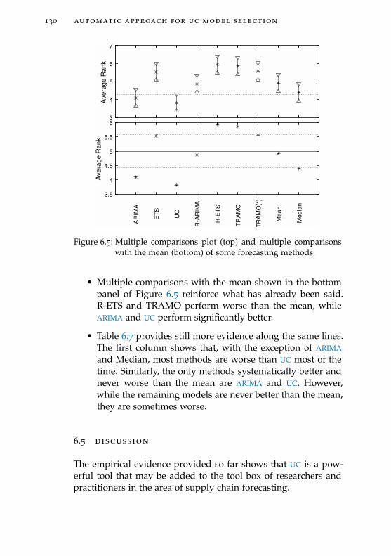
130 automatic approach for uc model selection
3
4
5
6
7
Ave
rag
e R
an
k
AR
IMA
ET
S
UC
R-A
RIM
A
R-E
TS
TR
AM
O
TR
AM
O(*
)
Mean
Media
n
3.5
4
4.5
5
5.5
6
Ave
rag
e R
an
k
Figure 6.5: Multiple comparisons plot (top) and multiple comparisonswith the mean (bottom) of some forecasting methods.
• Multiple comparisons with the mean shown in the bottompanel of Figure 6.5 reinforce what has already been said.R-ETS and TRAMO perform worse than the mean, whileARIMA and UC perform significantly better.
• Table 6.7 provides still more evidence along the same lines.The first column shows that, with the exception of ARIMA
and Median, most methods are worse than UC most of thetime. Similarly, the only methods systematically better andnever worse than the mean are ARIMA and UC. However,while the remaining models are never better than the mean,they are sometimes worse.
6.5 discussion
The empirical evidence provided so far shows that UC is a pow-erful tool that may be added to the tool box of researchers andpractitioners in the area of supply chain forecasting.
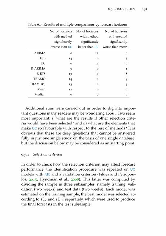
6.5 discussion 131
Table 6.7: Results of multiple comparisons by forecast horizons.
No. of horizons No. of horizons No. of horizons
with method with method with method
significantly significantly significantly
worse than UC better than UC worse than mean
ARIMA 0 12 0
ETS 14 0 3
UC 0 14 0
R-ARIMA 9 0 1
R-ETS 13 0 8
TRAMO 14 0 9
TRAMO(*) 13 0 4
Mean 12 0 0
Median 0 2 0
Additional runs were carried out in order to dig into impor-tant questions many readers may be wondering about. Two seemmost important: i) what are the results if other selection crite-ria would have been selected? and ii) what are the elements thatmake UC so favourable with respect to the rest of methods? It isobvious that these are deep questions that cannot be answeredfully in just one single study on the basis of one single database,but the discussion below may be considered as an starting point.
6.5.1 Selection criterion
In order to check how the selection criterion may affect forecastperformance, the identification procedure was repeated on UC
models with AIC and a validation criterion (Fildes and Petropou-los, 2015; Hyndman et al., 2008). This latter was computed bydividing the sample in three subsamples, namely training, vali-dation (two weeks) and test data (two weeks). Each model wasestimated on the training sample, the best model was selected ac-cording to sE7 and sE14 separately, which were used to producethe final forecasts in the test subsample.

132 automatic approach for uc model selection
Table 6.8 shows the median and 75% percentiles of sEh for thebest UC models according to SBC (as in Table 6.2), AIC (labeled as‘UC-AIC’) and both validation criteria (‘UC-VAL(7)’ for sE7 and‘UC-VAL(14)’ for sE14).
Selection based on AIC resulted in the same model than SBC
in 54.2% of all the cases and shows some marginal better perfor-mance than SBC. This is evidence in favour of AIC as a selectioncriterion, though obviously more research is necessary in order toconfirm or contradict these results, especially testing on differentdata sets.
Results are somewhat different regarding the validation crite-rion. Validation does not manage to produce better results thaninformation criteria, except for some very specific cases, beingthe behaviour for longer horizons worse than for shorter ones.Many more options may be tried out, like using different fore-casting horizons in this validation set up and/or other error met-rics. However, such exhaustive experiments are out of the scopeof this chapter.
6.5.2 Differences of Unobserved Components methods
The main general reason why UC shows superior performanceis because of their greater flexibility, at least in two ways: i) sea-sonal components are more flexible, since models with differentvariances and different noises for each separate harmonic are al-lowed; and ii) Multiple Source of Error (MSOE) SS systems areused, instead of Single Source of Error (SSOE) in innovations form,typical of ETS or ARIMA models.
There are other, less relevant differences. For example, the ex-act initialization of recursive algorithms in UC models is done inthis thesis as in Durbin and Koopman (2012), that theoreticallyare the same than ARIMA models estimated by Exact MaximumLikelihood and similar to ETS with estimation of initial states. An-other less important issue is the fact that different software, opti-mization routines, etc. are used.
The importance of using seasonal components with more thanone parameter and one noise has a long tradition in the UC litera-ture. The initial trigonometric approaches (Harrison and Stevens,

6.5 discussion 133
Table 6.8: Median and 75% percentile of sEh for different UC selectioncriteria.
Median 1 2 3 4 7 10 14
UC-SBC 0.211 0.223 0.228 0.230 0.232 0.237 0.243
UC-AIC 0.210 0.222 0.227 0.229 0.231 0.237 0.240
UC-VAL(7) 0.210 0.224 0.226 0.229 0.232 0.239 0.245
UC-VAL(14) 0.212 0.225 0.228 0.230 0.231 0.241 0.246
UC-FIX-SBC 0.214 0.226 0.230 0.233 0.236 0.243 0.248
75% perc. 1 2 3 4 7 10 14
UC-SBC 0.422 0.443 0.457 0.460 0.469 0.481 0.483
UC-AIC 0.422 0.444 0.457 0.460 0.467 0.481 0.483
UC-VAL(7) 0.420 0.445 0.457 0.465 0.472 0.488 0.488
UC-VAL(14) 0.426 0.448 0.461 0.467 0.474 0.483 0.492
UC-FIX-SBC 0.426 0.448 0.460 0.466 0.477 0.488 0.489
1976; Harvey, 1989) specified seasonal components with one com-mon variance parameter for a number of noises less or equal tothe fundamental period of the seasonal component (e.g., 6 fordaily data with weekly seasonality). That model was extendedlater, at least by Young, Pedregal, and Tych (1999) to one varianceparameter for each harmonic, on the basis of frequency domainarguments. Very often time series exhibit different spectral powerat different harmonic frequencies, even to the point that some ofthem do not show up at all. At least in those cases, giving thesame importance to all of them by a single parameter impliesestimating some sort of mean value, while estimating distinctparameters allows for a finer discrimination among different har-monics.
In order to test for the importance of this argument empirically,the forecast exercise was repeated forcing the seasonal compo-nents to have a single parameter (and independent noises) in allcases. The results are shown in the last row of Table 6.8 under la-bel ‘UC-FIX-SBC’. The models automatically identified were thesame in 51.8% of the cases, and the results show unequivocallythat the constrained model is worse, though still better in many

134 automatic approach for uc model selection
cases when compared with the rest of methodologies (compareresults with Table 6.5).
The final issue is whether the innovations form SSOE SS modelhas some advantages over the MSOE UC models. The SSOE SS formin which the ETS are cast by Hyndman et al. (2008) is quite con-venient in algorithmic terms since the states become observableand computations are much more efficient. In addition, it allowsto multiplicative extensions in an easy and brilliant way.
Proposing SSOE UC models might have at least two meanings:i) writing an MSOE model as an equivalent SSOE system as inCasals (2016) or finding its reduced form; or ii) constraining allthe noises in an UC model to be the same or behave with perfectcorrelation.
The former option is irrelevant to the discussion because theforecasts would be the same than the original UC model. The lat-ter option is shocking, at least contemplated from an UC formalpoint of view. In effect, constraining all the noises to be the samein a model like (6.6) implies imposing constraints that are still in-credibly more stringent than assuming just seasonal componentswith a single parameter and one noise for all harmonics. It is un-reasonable to think of components that ought to be constrainedin such wild way on a priori grounds and never has been pro-posed in the literature, to the knowledge of the authors. There iscertain literature on versions of UC models for trend-cycle decom-positions typical of macroeconomics with correlated components(references are very scarce for perfect correlation). Even in thosecases the conclusions about the convenience of correlated com-ponents are controversial, see e.g., Proietti (2006) and referencestherein.

7U N I F I E D A P P R O A C H F O R H I E R A R C H I C A LT I M E S E R I E S F O R E C A S T I N G .
7.1 overview and state of the art
Business and economic applications relying on time series areusually aggregated across geographic or logical dimensions toform hierarchical structures. The data is then forecast at differ-ent levels of aggregation which have been reported as beneficialin terms of robustness and accuracy. However, independent fore-casts of all time series at all levels of aggregation have the unde-sired property of being inconsistent across the hierarchy. There-fore, a strategy for reconciling forecasts across aggregation levelsto improve consistency is required.
Research on hierarchical time series have been reported in theliterature for several decades. Examples of early studies includeBarnea and Lakonishok (1980), Dangerfield and Morris (1992),Fliedner (1999), Gross and Sohl (1990), Grunfeld and Griliches(1960), Orcutt, Watts, and Edwards (1968), Shlifer and Wolff (1979),and Weatherford, Kimes, and Scott (2001); etc. In supply chainscenarios, for example, disaggregated demand data is usuallyavailable for every shop or distribution center. At this level, natu-ral hierarchies can be formed aggregating data corresponding tothe criteria of interest. Logical hierarchies can be formed whendata are grouped based on relevant criteria to the business. Fam-ilies (or groups) of products in grocery industries, for example,have an important role as a business variable for supply chain or-chestration (Fliedner and Lawrence, 1995; Muir, 1979). Synthetichierarchies can be defined simply by attending to the nature of
135
136 unified approach for hierarchical time series forecasting .
time series themselves. In these cases, time series are first classi-fied into groups according to their structural components so asto optimize modeling, and then are aggregated to form the nextlevel of the hierarchy (Fliedner, 2001).
A number of different approaches for optimizing hierarchicalforecasts have been proposed in recent years. The bottom-up ap-proach entails forecasting the lowest level in the hierarchy andpropagating the forecasts upwards according to the hierarchystructure (Dangerfield and Morris, 1992; Orcutt, Watts, and Ed-wards, 1968). The top-down strategy forecasts the uppermost leveltime series and then disaggregate down the forecasts to lowerlevels using different approaches, normally proration or by ra-tios of every single time series with respect to the aggregate,as described by Boylan (2010), Gross and Sohl (1990), and Strij-bosch, Heuts, and Moors (2008). Middle-out approach combinesboth previous approaches by forecasting a middle level and thenaggregating bottom-up as well as disaggregating top-down. Opti-mal reconciliation is proposed as a way of modifying individualforecasts and making them compatible, without the need to fixany of them on a priori grounds, the procedure has been alsoextended to temporal hierarchies (Athanasopoulos et al., 2017;Hyndman, Lee, and Wang, 2016; Hyndman et al., 2011). Recently,an allegedly new procedure appeared, known as integrated hier-archies, based on multivariate SS systems (Pennings and Dalen,2017).
Debate as to which approach is best in forecasting terms hasbeen going on for some time. Some studies are in favor of top-down approaches (Fliedner, 1999; Gross and Sohl, 1990; Grunfeldand Griliches, 1960), others prefer the bottom-up strategy (Danger-field and Morris, 1992; Orcutt, Watts, and Edwards, 1968; Weath-erford, Kimes, and Scott, 2001; Zellner and Tobias, 2000), whileothers advocate a reconciled approach (Hyndman, Lee, and Wang,2016; Hyndman et al., 2011). Some more theoretically orientedstudies have focused on analyzing the conditions under whichapproach produces more accurate forecasts than others (Lütke-pohl, 1984; Rostami-Tabar et al., 2016; Sbrana and Silvestrini, 2013;Shlifer and Wolff, 1979; Widiarta, Viswanathan, and Piplani, 2009).
7.1 overview and state of the art 137
At present, discussions remain inconclusive and will probablypersist over the following decades, for several reasons. Firstly, em-pirical comparisons suggest that there is no single approach thatoutperforms the rest, as the results depend on the complexity ofthe hierarchy, the quality of the data at each level, the accuracyof the models, etc. Secondly, setting out general conditions onwhich any hierarchy is better optimized on theoretical groundspresupposes ideal conditions that may or may not be met in ex-periments with real data, thus weakening importance for day today practice. Finally, discussions are becoming more complicatedbecause of the emergence of novel ways to optimize a hierarchy(for example, the reconciled approach). This chapter seeks to takethe debate a step further by proposing a new strategy to carry-ing out all the aggregation approaches, and for generalizing ahierarchy by defining each node type.
In this chapter, a SS approach for the general treatment of hier-archies is proposed, providing a framework that gives an unifiedsolution for top-down, bottom-up, middle-out and reconciled hierar-chical forecasting approaches. This framework permits a new cat-egory, combined, defined as any feasible logical combination ofthe aforementioned categories. In this framework, all the previ-ous cases are seen as particular examples of a combined hierarchy,in which each node is defined in any of such categories. In otherwords, our approach to the problem would consist on definingthe hierarchy structure and the type of each single node.
This approach improves upon recent research (mainly Hynd-man, Lee, and Wang, 2016; Hyndman et al., 2011) at least in twofundamental ways. Firstly, the appropriate SS form and the asso-ciated optimal recursive algorithms provide an elegant optimalsolution to the hierarchical forecasting problem without the needto turn up to any additional algebra. Secondly, given the recur-sive nature of the solution to the state estimation problem givenby the KF, the optimality is propagated along time, i.e., the so-lution preserves the time consistency implied by the individualmodels for each time series. This fact is completely disregardedin previous studies.
Time consistency is, on the contrary, taken into account in Pen-nings and Dalen (2017). But, though developed also in a SS frame-

138 unified approach for hierarchical time series forecasting .
work, the approach is rather different and more restricted thanthe one in this chapter. Certainly, it consists of a multivariate UC
or Structural model a la Harvey (Harvey, 1989) with componentsarbitrarily constrained, in which the hierarchical restrictions aretaken into account solely in a bottom-up manner. The univariatemodeling does not play any rule and no dynamical models areproposed for aggregated time series. In this chapter, other modelsthan UC are possible, all bottom-up, top-down and reconciled struc-tures are possible, dynamical models are specified for aggregatedseries and time consistency is preserved.
7.2 hierarchical forecasting
The problem of hierarchical forecasting consists in finding opti-mal forecasts for all the time series involved in a hierarchy in sucha way that the forecasts add up according to the constraints im-posed by the hierarchy. There are many types of hierarchies andeven more ways to organize the same data into different hierar-chies. The total sales of a company could be disaggregated firstinto regions and then in product families, or vice-versa, leadingto different hierarchies in each case. Figure 7.1 shows an exampleof a simple hierarchy, composed of three levels and eight nodesor time series, five of which are at the bottom level, as in Hynd-man, Lee, and Wang (2016).
A hierarchy may be represented as a multivariate model witha number of constraints. However, relevant hierarchies are as-sumed to be large, making their multivariate representation in-feasible. Thus, a more appropriate approach consists in identi-fying univariate models for each time series at every level in thehierarchy, and achieving forecast reconciliation in a second stage.
Any hierarchy or grouping data structure may be expressed asa linear transformation of the bottom level variables. The ensuingmatrix transforms the data or the forecasts at the bottom layerinto the whole data structure in a straightforward manner. Taking
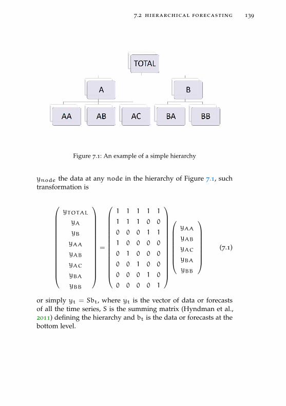
7.2 hierarchical forecasting 139
Figure 7.1: An example of a simple hierarchy
ynode the data at any node in the hierarchy of Figure 7.1, suchtransformation is
yTOTAL
yA
yB
yAA
yAB
yAC
yBA
yBB
=
1 1 1 1 1
1 1 1 0 0
0 0 0 1 1
1 0 0 0 0
0 1 0 0 0
0 0 1 0 0
0 0 0 1 0
0 0 0 0 1
yAA
yAB
yAC
yBA
yBB
(7.1)
or simply yt = Sbt, where yt is the vector of data or forecastsof all the time series, S is the summing matrix (Hyndman et al.,2011) defining the hierarchy and bt is the data or forecasts at thebottom level.

140 unified approach for hierarchical time series forecasting .
7.2.1 An example
A simple example is proposed here in order to illustrate the SS
approach. Let’s consider an ARMA(2, 1) model in Equation (7.2).
yt = φ1yt−1 +φ2yt−2 + εt + θεt−1, Var(εt) = σ2 (7.2)
The SS representation of this model is not unique, but one thatis often used in the literature is
(α1,t+1
α2,t+1
)=
(φ1 1
φ2 0
)(α1,t
α2,t
)+
(1
θ
)εt
yt =(1 0
)(α1,t
α2,t
) (7.3)
Matching system (7.3) with the general SS system (3.1) identi-fies the system matrices for this particular case, i.e.,
T =
(φ1 1
φ2 0
); R =
(1
θ
)εt Q = σ2
Z =(1 0
)C = 0 H = 0
Matrices T ,Q and R depend on the parameters of the ARMA(2,1)model and given the data may be estimated by Maximum Like-lihood. With the estimated values placed in these matrices, theKF in Chapter 3 gives the optimal estimation of the states, fore-casts and their covariances. Generalizations of this example toARMA(p,q) models is straightforward.
7.3 hierarchies in state space form
The problem stated in Section 7.2 may be solved by building anoverall SS system that comprises all the models in a hierarchywith the constraints imposed by the hierarchy structure and allthe information involved. It is assumed that the base models havebeen identified previously in some way, either automatically or

7.3 hierarchies in state space form 141
manually. In order to build the overall SS structure, such modelsought to be cast in SS form, though not necessarily identifiedwithin a SS framework.
The overall SS system representing the hierarchy is built in twosteps:
• Build up the overall system by block concatenation.
• Add hierarchical constraints depending on the type of hier-archy.
7.3.1 Build overall system
Assuming that the univariate models for all variables are set upin SS form, the model for the i-th variable may be written asin Equation (3.1) with a superscript ((i)) added to every singleelement in the SS formulation. Such superscript runs from 1 tothe number of variables k.
The first step, then, consists of building an overall SS systembased on k systems of type (3.1) (k = 8 in example of Figure 7.1).
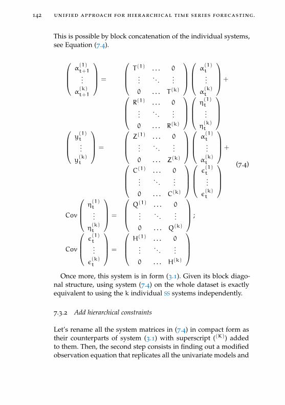
142 unified approach for hierarchical time series forecasting .
This is possible by block concatenation of the individual systems,see Equation (7.4).
α(1)t+1...
α(k)t+1
=
T (1) . . . 0
.... . .
...
0 . . . T (k)
α(1)t...
α(k)t
+
R(1) . . . 0
.... . .
...
0 . . . R(k)
η(1)t...
η(k)t
y(1)t...
y(k)t
=
Z(1) . . . 0
.... . .
...
0 . . . Z(k)
α(1)t...
α(k)t
+
C(1) . . . 0
.... . .
...
0 . . . C(k)
ε(1)t...
ε(k)t
Cov
η(1)t...
η(k)t
=
Q(1) . . . 0
.... . .
...
0 . . . Q(k)
;
Cov
ε(1)t...
ε(k)t
=
H(1) . . . 0
.... . .
...
0 . . . H(k)
(7.4)
Once more, this system is in form (3.1). Given its block diago-nal structure, using system (7.4) on the whole dataset is exactlyequivalent to using the k individual SS systems independently.
7.3.2 Add hierarchical constraints
Let’s rename all the system matrices in (7.4) in compact form astheir counterparts of system (3.1) with superscript ((K)) addedto them. Then, the second step consists in finding out a modifiedobservation equation that replicates all the univariate models and

7.3 hierarchies in state space form 143
the constraints imposed by the hierarchy at the same time. Thisis achieved by pre-multiplying the overall observation equationby a matrix S(∗), given in Equation (7.5).
S(∗) =(S(K) S
)(7.5)
Matrix S(∗) is actually a combination of matrix S that definesthe hierarchy structure and a new matrix S(K) that has to befound depending of the type of system (bottom-up, etc.). The di-mension of S(K) is k×m, where m is the number of aggregatedvariables.
• Bottom-up: S(K) = 0. Pre-multiplying the observation equa-tion by S(∗) in this case leaves the system as it is. In thiscase, forecasts may be produced simply as the aggregationof individual forecasts without any need of the overall sys-tem. A more efficient version of this model, with less states,is found by declaring S(K) as an empty matrix and using anoverall system that only comprises the models at the bottomlevel. Indeed, this is the preferred form when the system ispurely bottom-up. However, this less efficient version is pre-ferred for the sake of the combined systems defined below.
• Top-down: as in the case of bottom-up, but inserting the fore-casts obtained by the individual model of yTOTAL as actualdata. As in the previous case, the top-down system may bedefined more efficiently with less states, but this form isretained.
• Reconciled: S(K) =(
−I 0
) ′, where I is an identity matrix
of a dimension equal to the number of aggregated variables(m) and the rest are a block of zeros of appropriate dimen-sion ((k −m)×m). In this case, y(K)t is a composition ofzeros for the aggregated data and the disaggregated seriesbt.
• Combined: the way each case above is set up allows for theircombination in a single hierarchy by selecting appropriate
144 unified approach for hierarchical time series forecasting .
values for the diagonal elements of matrix S(K) and the dataaffecting it. For example, by setting S(K)(i, i) = −1 and ze-ros for the i− th aggregate variable that node is chosen asreconciled. Otherwise, set S(K)(i, i) = 0 and missing dataor the forecasts of the univariate model for i − th aggre-gated series, for bottom-up or top-down options, respectively.One must bear in mind that the middle-out case quoted inthe literature is just a particular case of a combined hierar-chy. Therefore, rather than speaking about hierarchy types(i.e., bottom-up, reconciled, etc.) a thorougher nomenclaturewould be to talk of node types.
7.3.3 Discussion
The path followed to build the SS hierarchical system illustrateshow the transition equation embodies the dynamical systemsof all the independent univariate models, while the observationequation just defines both the hierarchy structure and node types.Thus, the two-step KF in Chapter 3 renders the optimal one-step-ahead forecasts of the states: in the prediction step, which onlyuses the transition equation system matrices, the independentforecasts are computed regardless of the hierarchy, while thecorrection step updates them by imposing the appropriate con-straints according to the hierarchy structure. Such a correction isdone by minimizing the MSE, conditional on all information avail-able at any time, on the univariate models for all series and onthe constraints imposed by the hierarchy.
An additional benefit of this approach is that it neatly takesadvantage of the KF optimality without any further assumptionsor any further algebra. In the particular case of the top-down sys-tems, there is no need to elaborate on how the top forecasts haveto be disaggregated (Gross and Sohl, 1990). The advantages alsoapply to reconciled systems, in which additional objective func-tions ought to be assumed, opening the door to different options(Hyndman, Lee, and Wang, 2016; Hyndman et al., 2011).
Still more important is the fact that any hierarchical forecastsare produced based on past optimal forecasts obtained with thehierarchy and the forecasts are consistent both hierarchical-wise

7.3 hierarchies in state space form 145
and time-wise, i.e., with the constraints imposed by the hierarchyand the time dynamics of the univariate models optimally identi-fied. Clearly this is not the case of the Hyndman et al. (2011) ap-proach, where the reconciled forecasts are produced based solelyon the initial univariate/independent forecasts without any refer-ence to the previous reconciled forecasts, losing the consistencyacross the temporal dimension. The top-down approach has simi-lar consistency problems along time.
The following simple example illustrates the point of time con-sistency of the SS reconciled forecasts. Let’s assume two indepen-dent AR(1) processes,
x1,t = 0.8x1,t−1 + a1,t, var(a1,t) = 1
x2,t = −0.8x2,t−1 + a2,t, var(a2,t) = 1(7.6)
It is well known that the eventual forecast function of both pro-cesses decay exponentially to zero, the first one from either thepositive or negative side, while the second alternates sign aroundzero. The aggregation of the two processes (yt = x1,t + x2,t) isan AR(2) because the coefficients of the two AR(1) processes areequal and opposite in sign and the variance of both noises isthe same (Granger and Morris, 1976). A simulation of the abovemodels produces forecasts like the ones shown in Figure 7.2. Thestandard procedure is done in the R environment with the htspackage (Hyndman et al., 2011), while the SS forecasts are donein MATLAB with the SSpace toolbox (Villegas and Pedregal, 2018
and Chapter 4). The example is done in a way such that the baseAR models are exactly the same in both cases, making sure thatthe observed differences are strictly and solely due to the aggre-gation procedures. The SS reconciled forecasts resemble what isexpected in theory, while the standard procedure produces fore-casts that are combinations of the expected. In this sense, SS ap-proach is time-consistent, while the standard method computedwith hts package is not.
The possibilities of combined systems open up the door to fur-ther considerations. Taking the hierarchy in Figure 7.1, the ad-justed forecasts will be different depending on the type assigned

146 unified approach for hierarchical time series forecasting .
Figure 7.2: Forecasts of a simulation of aggregation of two AR(1) systems
to each node. Figure 7.3 shows just a few possibilities that nat-urally differ from those in which all the nodes are of the sametype. Then, for the same hierarchy there are many different waysto produce forecasts, all optimal from the point of view of min-imizing the mean squared error, but with different sets of infor-mation/constraints. The selection of each node type may be car-ried out by a lengthy empirical process, resembling data miningprocedures, or by imposing constraints based on previous expe-rience. Not every possible combination is logical, but the numberof logical combinations is certainly very high, increasing with thenumber of nodes and the depth and width of the hierarchy. Thisis an area that requires more research and is beyond the scope ofthis chapter.
Kahn (1998) mentioned the idea of a hybrid approach combin-ing the advantages of top-down and bottom-up. As previously dis-cussed, our approach provides a framework that takes this ideaof flexibility to a new extent, allowing to assign a combinationstrategy to each node in the hierarchy. Moreover, further consid-erations are:
• The proposed approach makes it easy to integrate multivari-ate models as part of the hierarchy. Instead of a block con-

7.4 simulations 147
Figure 7.3: Some of the possible options for the top structure of the hier-archy in Figure 7.1. TD, BU and R stand for top-down, bottom-up and reconciled, respectively.
catenation of univariate models, the corresponding blockwould be replaced by the appropriate multivariate module.
• Judgmental forecasts may be incorporated into the hierar-chy at any node by selecting them as a top-down node.
• Node types may be also time dependent, keeping the hier-archy and time consistency and building forecasts on pastoptimal forecasts based on the hierarchy structure. A sys-tem might be bottom-up at some points in time and top-downat others, meaning that by means of the latter the forecastsare forced to reach a certain level at certain time stamps.
• Simulations are also possible, for example, it is possible toset scenarios to answer questions such us what future pathsare compatible with certain future values at certain nodes.
• Optimal confidence bands or prediction intervals may beestimated automatically from the standard KF output in theusual way.
7.4 simulations
In this section we develop a simulation study to compare theproposed methodology with existing alternatives. The simulationprocess is basically a replication of the one described in Hynd-man et al. (2011) with minor modifications. All bottom level seriesare simulated as ARIMA(p,d,q) processes with d = 1, p ∈ (0, 2)and q ∈ (0, 2) with parameter values chosen randomly with equal
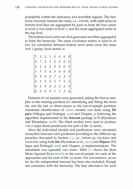
148 unified approach for hierarchical time series forecasting .
probability within the stationary and invertible regions. The hier-archy structure remains the same, i.e., 3 levels, with eight series atbottom-level that are aggregated by pairs to form the four seriesat level 2, two series at level 1, and the most aggregated series atthe top level.
The bottom-level series are first generated and then aggregatedto form the hierarchy. The same covariance matrix is used to al-low for correlation between bottom level series from the samelevel 1 group. Such matrix is
7 3 2 1 0 0 0 0
3 7 2 1 0 0 0 0
2 2 6 3 0 0 0 0
1 1 3 6 0 0 0 0
0 0 0 0 7 3 2 1
0 0 0 0 3 7 2 1
0 0 0 0 2 2 6 3
0 0 0 0 1 1 3 6
Datasets of 100 samples were generated, taking the first 90 sam-
ples as the training partition for identifying and fitting the mod-els, and the last 10 observations as the out-of-sample partition.Automatic identification of ARIMA models was done using SS-pace (Villegas and Pedregal, 2018 and Chapter 4) following thealgorithm implemented in the forecast package in R (Hyndmanand Khandakar, 2008). The fitted models were used to produce1-to-7 steps-ahead predictions for each of the 15 series.
Once the individual models and predictions were calculated,reconciled forecasts were produced according to the different ap-proaches discussed in Section 7.3, i.e., bottom-up, top-down andreconciled, using both hts (Hyndman et al., 2011) and SSpace (Vil-legas and Pedregal, 2018 and Chapter 4) implementations. Thesimulation was repeated 1000 times. Table 7.1 shows the RootMean Squared Error (RMSE) in the out-of-sample for each of theapproaches and for each of the 15 series. For convenience, an en-try for the independent forecast has been also included, thoughnot consistent with the hierarchy. The best alternative for each

7.4 simulations 149
Table 7.1: RMSE for out-of-sample forecasting of the simulated data. Ind.stands for Independent, BU for bottom-up and TD for top-down.
Ind. BU TD Reconciled
hts sspace hts sspace
Total 28.59 24.30 28.59 28.59 26.66 24.63
A 18.50 16.64 35.28 18.50 17.97 16.89
B 18.93 16.88 34.95 18.74 18.42 17.24
AA 11.19 10.58 24.89 11.43 11.05 10.62
AB 10.78 9.86 25.05 10.83 10.70 10.09
BA 11.18 10.59 26.60 11.64 11.35 10.77
BB 10.58 9.71 28.95 10.37 10.54 9.88
AAA 6.01 6.01 15.92 6.42 6.32 6.11
AAB 6.54 6.54 21.39 6.99 6.77 6.48
ABA 5.88 5.88 16.28 6.39 6.30 5.93
ABB 5.76 5.76 17.52 6.18 6.23 5.95
BAA 6.25 6.25 19.85 6.76 6.61 6.33
BAB 6.19 6.19 22.43 6.72 6.59 6.28
BBA 5.69 5.69 29.05 6.00 6.12 5.77
BBB 5.72 5.72 24.85 6.02 6.12 5.77
Average 10.52 9.77 24.77 10.77 10.52 9.91
horizon and level is shown in bold. Since the bottom-up approachsimply aggregates the bottom level forecasts all the way to thetop level, results are equivalent for both hts and SSpace and theyare shown in a single entry. On the other hand, different resultsare drawn for top-down and reconciled strategies, and RMSE valuesare shown separately for each implementation.
One important point is that all models automatically identifiedare exactly the same in both implementations (hts and SSpace).Thence, the accuracy differences observed in Table 7.1 are onlydue to the differences in reconciling approaches.

150 unified approach for hierarchical time series forecasting .
Since random ARIMA processes were used both to generate theseries and (automatically) identify the models, the bottom-up strat-egy results favored, explaining its good performance. However,the value of this particular setup relays on providing a com-mon ground for comparing existing approaches (hts) with theproposed approach (SSpace), leaving apart the aforementioneddiscussion on top-down vs bottom-up. The mean RMSE value forbottom-up (9.77) is indeed the best of all, even better than the in-dependent forecasts (10.52 mean RMSE).
Some observations can be highlighted from Table 7.1. Regard-ing global averages (last row), results seem to be scattered aroundthe independent (Ind.) forecasts (10.52), except for top-down[hts]value sitting apart (24.77), a finding in common with Hyndmanet al. (2011). Reconciled[sspace] method (9.91) outperforms all al-ternatives except bottom-up (9.77), including the independent base-line (10.52).
Regarding top-down and reconciled approaches, SSpace system-atically provides better results than the counterpart in hts forall series. This result comes to support the claim about the con-venience of keeping consistency across time while reconcilingacross hierarchy. As previously discussed in Section 7.3, the pro-posed approach for reconciling forecasts also maintains consis-tency with models across time, which is expected to increase co-herence and performance of the final system.
Pairwise t-tests for the 6 approaches were computed. As ex-pected from results in Table 7.1, top-down[hts] vs the rest returneda p-value smaller than 10−8 for all possible comparisons. Thebest of all approaches is the bottom-up (being consistent with theexperiment design as previously discussed) which compared toindependent is said to be different with 99% of confidence (p-value5.2×10−4), but not significantly different from reconciled[sspace](p-value 0.51). Finally, both reconciled approaches are differentwith 99% of confidence (p-value 7× 10⁻³).
7.5 hierarchical demand forecasting
In this section we apply the proposed approach to predict thedemand of a Spanish grocery retailer. The dataset contains daily
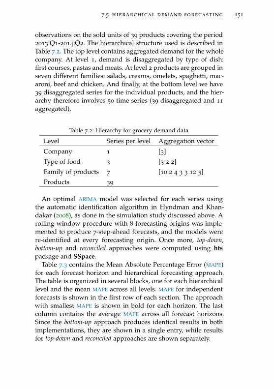
7.5 hierarchical demand forecasting 151
observations on the sold units of 39 products covering the period2013:Q1-2014:Q2. The hierarchical structure used is described inTable 7.2. The top level contains aggregated demand for the wholecompany. At level 1, demand is disaggregated by type of dish:first courses, pastas and meats. At level 2 products are grouped inseven different families: salads, creams, omelets, spaghetti, mac-aroni, beef and chicken. And finally, at the bottom level we have39 disaggregated series for the individual products, and the hier-archy therefore involves 50 time series (39 disaggregated and 11
aggregated).
Table 7.2: Hierarchy for grocery demand data
Level Series per level Aggregation vector
Company 1 [3]
Type of food 3 [3 2 2]
Family of products 7 [10 2 4 3 3 12 5]
Products 39
An optimal ARIMA model was selected for each series usingthe automatic identification algorithm in Hyndman and Khan-dakar (2008), as done in the simulation study discussed above. Arolling window procedure with 8 forecasting origins was imple-mented to produce 7-step-ahead forecasts, and the models werere-identified at every forecasting origin. Once more, top-down,bottom-up and reconciled approaches were computed using htspackage and SSpace.
Table 7.3 contains the Mean Absolute Percentage Error (MAPE)for each forecast horizon and hierarchical forecasting approach.The table is organized in several blocks, one for each hierarchicallevel and the mean MAPE across all levels. MAPE for independentforecasts is shown in the first row of each section. The approachwith smallest MAPE is shown in bold for each horizon. The lastcolumn contains the average MAPE across all forecast horizons.Since the bottom-up approach produces identical results in bothimplementations, they are shown in a single entry, while resultsfor top-down and reconciled approaches are shown separately.

152 unified approach for hierarchical time series forecasting .
Some ideas emerge from this empirical study: (1) the bottom-upstrategy is systematically out-performed in all horizons and lev-els by either top-down or reconciled approaches. (2) As we movedown in the hierarchy, the reconciled approach excels at longerhorizons (5, 6 and 7 steps ahead), while the top-down approachdoes better at shorter horizons (1, 2 and 3 steps ahead). (3) TheSSpace approach seems to systematically out-perform hts imple-mentation for longer horizons (4, 5, 6 and 7 steps ahead) bothin top-down and reconciled approaches, while hts work better atshorter horizons in both approaches as well (with some excep-tions, see for example Level 1 of Table 7.3).

7.5 hierarchical demand forecasting 153
Table 7.3: MAPE for out-of-sample forecasting of the alternative hierarchi-cal approaches applied to a Spanish retailer demand data.
Forecast horizon
1 2 3 4 5 6 7 AVG
Top level
Independent 6.86 7.94 7.99 15.29 16.23 15.71 15.54 12.22
Bottom-up 7.48 9.90 9.78 16.41 17.68 17.07 17.00 13.62
Top-down hts 6.86 7.94 7.99 15.29 16.23 15.71 15.54 12.22
sspace 6.86 7.94 7.99 15.29 16.23 15.71 15.54 12.22
Reconciled hts 6.87 7.97 7.82 15.17 16.20 15.76 15.48 12.18
sspace 7.07 8.92 10.48 17.86 17.22 15.59 14.94 13.15
Level 1
Independent 9.44 10.70 10.34 17.29 18.80 18.98 17.42 14.71
Bottom-up 10.66 12.53 12.86 19.29 20.19 19.16 18.06 16.11
Top-down hts 9.66 10.63 10.77 17.51 18.88 18.89 17.29 14.80
sspace 9.69 9.61 10.08 17.02 17.59 16.80 15.67 13.78
Reconciled hts 9.68 10.83 10.87 17.52 18.87 18.84 17.25 14.84
sspace 10.44 11.28 12.51 17.83 16.71 15.16 14.38 14.04
Level 2
Independent 13.28 14.47 15.39 22.08 22.56 23.55 21.42 18.96
Bottom-up 15.10 17.20 18.24 24.44 25.44 25.36 23.69 21.35
Top-down hts 13.33 13.99 14.95 22.32 22.83 23.64 21.37 18.92
sspace 16.23 17.48 17.36 22.70 23.93 23.42 21.54 20.38
Reconciled hts 13.48 14.68 14.91 22.37 23.07 23.78 21.45 19.11
sspace 15.23 17.19 17.44 22.27 21.64 20.60 19.14 19.07
Bottom level
Independent 28.09 30.19 31.99 36.80 37.23 37.72 35.95 33.99
Bottom-up 28.09 30.19 31.99 36.80 37.23 37.72 35.95 33.99
Top-down hts 27.68 29.42 30.67 36.31 36.48 37.12 35.12 33.26
sspace 31.41 31.72 32.55 36.43 36.69 36.15 34.58 34.22
Reconciled hts 27.99 30.44 31.52 37.46 37.98 38.67 36.43 34.36
sspace 29.82 30.55 31.30 35.43 34.96 34.29 33.31 32.81
Average
Independent 24.48 26.37 27.89 33.14 33.65 34.17 32.39 30.30
Bottom-up 24.82 26.90 28.47 33.61 34.16 34.46 32.78 30.74
Top-down hts 24.17 25.71 26.82 32.81 33.11 33.71 31.74 29.72
sspace 27.49 27.93 28.58 32.92 33.35 32.80 31.24 30.62
Reconciled hts 24.44 26.61 27.48 33.71 34.31 34.94 32.77 30.61
sspace 26.16 27.09 27.82 32.18 31.64 30.85 29.82 29.37


Part IV
C O N C L U S I O N S


8C O N C L U S I O N S
Business Analytics (BA) are spreading across all industries. Asthe amount of business data exponentially grows everyday, it iscritical to have appropriate tools that make it possible to con-sume and take profit of this digital universe. Even though BA
tools have positively evolved in this direction, meaningful andproductive use of data still remains a major obstacle for mostorganizations. Of drowning in data, they have moved to drownin reports, dashboards and data summaries. We believe that BA
technologies should evolve towards a more holistic approach inwhich business users can focus on business concepts and ques-tions, without wasting time in lower levels of cumbersome datamanipulation.
In Chapter 2 we propose the BA architecture as the infrastruc-ture supporting ’smart’ and enterprise BA operations. It enablesusers to define the business concepts they want to focus on, aswell as connecting them with data at storage level. Analytical anddata-mining algorithms are intensively exploited, all guided bythe ’semantic layer’ previously depicted by business users. Chap-ter 2 provides a general overview of the BA issue to serve as aframework to which the rest of the thesis make some concretecontributions. Actually, it is argued that BA is considered as theinfrastructure enabling users to define the business concepts theywant to focus on, as well as connecting them with data at storagelevel.
The rest of the thesis concentrates on much more concrete as-pects related to BA, in an attempt to bridge the gap between theraw data and making sense of them in a very specific context,
157

158 conclusions
namely the analysis and forecasting of big time series data basestypical of BA. For this purpose, and still more concretely, Chapter3 shows the main theory on which SS systems relies on. This isthe very bottom line on which the rest of the thesis rests.
In order to provide our potential audience with a softwarepackage to perform this sort of advanced analysis, Chapter 4
presents SSpace, a new toolbox for the exploitation of SS models.It is intended for a wide audience, including professional practi-tioners, researchers and students, indeed anyone involved in theanalysis of time series, forecasting or signal processing.
The library incorporates most of modern algorithms and ad-vances in the field of SS modeling, described in Chapter 3. Thesystem is very general because it is possible to implement linear,non-Gaussian and non-linear systems, all system matrices mayvary over time and may be multivariate, several estimation meth-ods are implemented, inputs to the system may be introducedexplicitly, etc.
Other advantages of the library are that a few functions are nec-essary to carry out a comprehensive analysis of time series. Suchfunctions are used systematically following a fixed pattern thatsimplifies the usage of the toolbox. However, one of the main fea-ture that makes SSpace really flexible, powerful and transparentis that the user implements models directly as a function writ-ten in MATLAB. This approach makes some cumbersome taskstruly simple and transparent. This is the case, say of trying differ-ent parameterizations of the same model or imposing parameterconstraints.
The toolbox is supplied with templates for building general SS
models from scratch in a completely free way, but is also accom-panied by a number of templates useful for the implementationof a variety of common models.
The capabilities of the toolbox have been demonstrated in ac-tion on several worked examples. These properties should makethe toolbox particularly interesting for those in need of non-standardmodels, for which even many commercial alternatives may notprovide the required flexibility.
Chapters 5 and 6 make some contribution to the field of au-tomatic identification. On the one hand, in Chapter 5 a general
conclusions 159
approach for model selection is proposed on the basis of Sup-port Vector Machines. On the other hand, Chapter 6 focuses on amuch more concrete contribution consisting of a novel automaticidentification procedure for UC models.
The procedure of Chapter 5 consists of selecting the best fore-cast model available from a pool of alternatives at each point intime by means of a SVM trained in a feature space that embeds themost recent information, forecasts, the relative performance andfitted parameters of the models involved. As far as the authorsare concerned, this is the first time SVM are used in this contextin this particular way.
The approach is empirically applied to a leading householdand personal care UK manufacturer with 229 weekly SKU to fore-cast, with a horizon of 1 to 4 weeks ahead. Findings suggest that:i) ETS techniques are very good in this context both in terms offorecast accuracy and minimization of bias, maybe a reason whythis is the technique most used in industry and business; ii) sim-ple combination of forecasts (like mean and median) do not helpmuch in this regard; iii) SVM-based model selection certainly man-age to improve the forecasting results, both in terms of errors andbias.
The specific model selection approach shown in Chapter 6 con-tribute to solve the challenges of the efficient and robust auto-matic handling of massive databases. For that aim, a general Au-tomatic Forecasting Support System built upon UC models withinthe unified framework provided by SS methods shown in chap-ters 3 and 4. As far as the authors know, this is the first time UC
models have been proposed in a supply chain forecasting con-text, and this is also the first time automatic identification of UC
models has been proposed.A comprehensive evaluation of the system shows that UC mod-
els compete very favorably with other standard alternatives inforecasting terms. This is true for all the models estimated bythe toolbox, implying that UC is slightly better than ARIMA andsignificantly better than ETS.
The results are consistent when the same models are estimatedwith alternative, well-established software packages, which points
160 conclusions
to the quality of the software developed and the usefulness of UC
models as forecasting devices in the area.Most importantly, significant differences among methods are
also outlined. In particular, UC is significantly better than ETS,invalidating, or at least discrediting, the idea that UC models are“similar” to ETS. However, UC is also better than ARIMA modelsestimated with other software, but very similar to ARIMA in thetoolbox. In a few words, this approach provides a starting pointfor considering UC models as a competitive method with greatpotential in this and other fields.
Finally, Chapter 7 shows a new approach for hierarchical timeseries forecasting based on SS modeling. The method gives anunified solution for top-down, bottom-up, middle-out and reconciledhierarchical forecasting approaches.
In this way, the hierarchical forecasting problem is convertedinto a standard SS problem for which the KF provides an optimalsolution. This fact simplifies the assumptions on which the ap-proach relies on. In particular, there is no need to add any wayto disaggregate down in top-down approaches, or to propose anyadditional objective function typical of reconciled approaches.
Most importantly, due to the use of the KF, the solution pre-serves the time consistency of the forecasts, a property that ismissing in most of the previous approaches. Moreover, forecastsare always produced on the basis of past optimal forecasts, in-stead on the raw individual forecasts, enhancing the coherencyof the approach. The SS framework permits the generalization ofthe problem by defining the type of each single node in a hierar-chy by means of combined hierarchies. Such heterogeneity may beeven time-varying, if required. Confidence intervals or predictionintervals may be built with the aid of the standard output of theKF.
The new approach is evaluated on simulations and on real dataof a Spanish grocery retailer. Both experiments show that the pro-posed approach provides significantly better results than existingapproaches.

B I B L I O G R A P H Y
Adya, M, F Collopy, JS Armstrong, and M Kennedy (2001). “Au-tomatic identification of time series features for rule-basedforecasting.” In: International Journal of Forecasting 17.2, pp. 143
–157. issn: 0169-2070.Athanasopoulos, G, RJ Hyndman, H Song, and DC Wu (2011).
“The tourism forecasting competition.” In: International Jour-nal of Forecasting 27.3, pp. 822–844.
Athanasopoulos, T, RJ Hyndman, N Kourentzes, and F Petropou-los (2017). “Forecasting with temporal hierarchies.” In: Euro-pean Journal of Operational Research 262.1, pp. 60–74.
Barnea, A and J Lakonishok (1980). “An analysis of the usefulnessof disaggregated accounting data for forecasts of corporateperformance.” In: Decision Sciences 11.1, pp. 17–26.
Barone, D, E Yu, J Won, L Jiang, and J Mylopoulos (2010a). “En-terprise modeling for business intelligence.” In: pp. 31–45.
Barone, D, J Mylopoulos, L Jiang, and D Amyot (2010b). “Thebusiness intelligence model: Strategic modelling.” In:
Barrow, DK and N Kourentzes (2016). “Distributions of Forecast-ing Errors of Forecast Combinations: Implications for Inven-tory Management.” In: International Journal of Production Eco-nomics 177, pp. 24–33.
Billah, B, ML King, RD Snyder, and AB Koehler (2006). “Expo-nential smoothing model selection for forecasting.” In: Inter-national Journal of Forecasting 22.2, pp. 239 –247. issn: 0169-2070.
Bossche, FV (2011). “Fitting State Space Models with EViews.”In: Journal of Statistical Software 41.8, pp. 1–16. doi: 10.18637/jss.v041.i08.
Box, GEP, GM Jenkins, GC Reinsel, and GM Ljung (2015). Timeseries analysis: forecasting and control. John Wiley & Sons.
Boylan, JE (2010). “Choosing levels of aggregation for supplychain forecasts.” In: Foresight 18, pp. 9–13.
161

162 Bibliography
Brown, RG (1959). Statistical Forecasting for Inventory Control. McGraw-Hill.
Buytendijk, F (2010). Dealing with dilemmas: Where business analyt-ics fall short. John Wiley & Sons.
Cao, LJ, KS Chua, WK Chong, HP Lee, and QM Gu (2003). “Acomparison of PCA, KPCA and ICA for dimensionality re-duction in support vector machine.” In: Neurocomputing 55.1,pp. 321–336.
Casals, J (2016). State-space methods for time series analysis : the-ory, applications and software. Monographs on statistics andapplied probability (Series) 149. CRC Press.
Casals, JM, A Garcia-Hiernaux, M Jerez, S Sotoca, and AA Trindade(2016). State-Space Methods for Time Series Analysis: Theory, Ap-plications and Software. Chapman and Hall/CRC.
Chen, PPS (1976). “The entity-relationship model—toward a uni-fied view of data.” In: ACM Transactions on Database Systems(TODS) 1.1, pp. 9–36.
Clemen, RT (1989). “Combining forecasts: A review and anno-tated bibliography.” In: International Journal of Forecasting 5.4,pp. 559 –583. issn: 0169-2070.
Collopy, F and JS Armstrong (1992). “Rule-Based Forecasting: De-velopment and Validation of an Expert Systems Approach toCombining Time Series Extrapolations.” In: Management Sci-ence 38.10, pp. 1394–1414.
Commandeur, JJF, SJ Koopman, and M Ooms (2011). “StatisticalSoftware for State Space Methods.” In: Journal of StatisticalSoftware 41.1, pp. 1–18. doi: 10.18637/jss.v041.i01.
Cortes, C and V Vapnik (1995). “Support-vector networks.” In:Machine learning 20.3, pp. 273–297.
Croston, JD (1972). “Forecasting and stock control for intermit-tent demands.” In: Operational Research Quarterly 23, pp. 289–303.
Cukier, K (2010). Data, data everywhere: A special report on managinginformation. Economist Newspaper.
Dangerfield, BJ and JS Morris (1992). “Top-down or bottom-up:Aggregate versus disaggregate extrapolations.” In: Interna-tional Journal of Forecasting 8.2, pp. 233 –241.

Bibliography 163
Davenport, TH and JG Harris (2007). Competing on analytics: thenew science of winning. Harvard Business Press.
Davidenko, A and R Fildes (2013). “Measuring forecasting ac-curacy: The case of judgmental adjustments to SKU-leveldemand forecasts.” In: International Journal of Forecasting 29,pp. 510–522.
Davidenko, A and R Fildes (2016). “Forecast Error Measures: Crit-ical Review and Practical Recommendations.” In: BusinessForecasting: Practical Problems and Solutions. John Wiley & SonsInc.
De Gooijer, JG and RJ Hyndman (2006). “25 years of time seriesforecasting.” In: International Journal of Forecasting 22, pp. 443–473.
Decker, G, R Dijkman, M Dumas, and L García-Bañuelos (2010).“The Business Process Modeling Notation.” In: Modern Busi-ness Process Automation. Springer, pp. 347–368.
Doan, T (2011). “State Space Methods in RATS.” In: Journal ofStatistical Software 41.9, pp. 1–16. doi: 10.18637/jss.v041.i09.
Drukker, R and R Gates (2011). “State Space Methods in Stata.”In: Journal of Statistical Software 41.10, pp. 1–25. doi: 10.18637/jss.v041.i10.
Duin, RPW and M Loog (2004). “Linear dimensionality reduc-tion via a heteroscedastic extension of LDA: the Chernoffcriterion.” In: IEEE transactions on pattern analysis and machineintelligence 26.6, pp. 732–739.
Durbin, J and SJ Koopman (2012). Time series analysis by state spacemethods. 38. Oxford University Press.
Fildes, R (1989). “Evaluation of Aggregate and Individual Fore-cast Method Selection Rules.” In: Management Science 35.9,pp. 1056–1065. eprint: http://dx.doi.org/10.1287/mnsc.35.9.1056.
Fildes, R and F Petropoulos (2015). “Simple versus complex se-lection rules for forecasting many time series.” In: Journal ofBusiness Research 68.8. Special Issue on Simple Versus Com-plex Forecasting, pp. 1692 –1701. issn: 0148-2963.
164 Bibliography
Fildes, R, N Nikolopoulos, SF Crone, and Syntetos AA (2008).“Forecasting and operational research: a review.” In: Journalof the Operational Research Society 59, pp. 1150–1172.
Fliedner, EB and B Lawrence (1995). “Forecasting system parentgroup formation: An empirical application of cluster analy-sis.” In: Journal of Operations Management 12.2, pp. 119–130.issn: 02726963. doi: 10.1016/0272-6963(94)00009-4.
Fliedner, G (1999). “An investigation of aggregate variable timeseries forecast strategies with specific subaggregate time se-ries statistical correlation.” In: Computers & Operations Re-search 26.10, pp. 1133 –1149.
Fliedner, G (2001). “Hierarchical forecasting: Issues and use guide-lines.” In: Industrial Management & Data Systems 101.1, pp. 5–12.
Furey, TS, N Cristianini, N Duffy, D W Bednarski, M Schummer,and D Haussler (2000). “Support vector machine classifica-tion and validation of cancer tissue samples using microar-ray expression data.” In: Bioinformatics 16.10, pp. 906–914.
Gardner, ES (1985). “Exponential smoothing: The state of the art.”In: Journal of Forecasting 4, pp. 1–28.
Gardner, ES (2006). “Exponential smoothing: The state of the art -Part II.” In: International Journal of Forecasting 22, pp. 637–666.
Gómez, V and A Maravall (2001). “Automatic Modeling Methodsfor Univariate Series.” In: A Course in Time Series. John Wiley& Sons, Inc., pp. 171–201.
Granger, CWJ and MJ Morris (1976). “Time series modelling andinterpretation.” In: Journal of the Royal Statistical Society. SeriesA 139.2, pp. 246–257.
Gross, CW and JE Sohl (1990). “Disaggregation methods to expe-dite product line forecasting.” In: Journal of Forecasting 9.3.
Grunfeld, Y and Z Griliches (1960). “Is Aggregation NecessarilyBad?” In: The Review of Economics and Statistics 42.1, pp. 1–13.
Gómez, V (2015). “SSMMATLAB: A Set of MATLAB Programs forthe Statistical Analysis of State Space Models.” In: Journal ofStatistical Software 66.9, pp. 1–37. doi: 10.18637/jss.v066.i09.

Bibliography 165
Han, J, E Haihong, G Le, and J Du (2011). “Survey on NoSQLdatabase.” In: Pervasive computing and applications (ICPCA),2011 6th international conference on. IEEE, pp. 363–366.
Harrison, PJ and CF Stevens (1976). “Bayesian Forecasting.” In:Journal of the Royal Statistical Society. Series B (Methodological)38, pp. 205–247.
Harvey, AC (1989). Forecasting, structural time series models and theKalman filter. Cambridge university press.
Hastie, T, R Tibshirani, and J Friedman (2009). The elements ofstatistical learning: data mining, inference, and prediction. NewYork: Springer Publishing.
Haykin, S (2008). Neural networks and learning machines. New Jer-sey: Prentice Hall.
Hira, Z M and DF Gillies (2015). “A review of feature selectionand feature extraction methods applied on microarray data.”In: Advances in bioinformatics 2015.
Hocking, RR (1976). “The Analysis and Selection of Variables inLinear Regression.” In: Biometrics 32, pp. 1–49.
Huang, CL, MC Chen, and CJ Wang (2007). “Credit scoring witha data mining approach based on support vector machines.”In: Expert Systems with Applications 33.4, pp. 847 –856. issn:0957-4174. doi: 10.1016/j.eswa.2006.07.007. url: http://www.sciencedirect.com/science/article/pii/S095741740600217X.
Hyndman, R, AB Koehler, JK Ord, and RD Snyder (2008). Fore-casting with exponential smoothing: the state space approach. SpringerScience & Business Media.
Hyndman, RJ and Y Khandakar (2008). “Automatic Time SeriesForecasting: The Forecast Package for R.” In: Journal of Statis-tical Software 3.27, pp. 1–22.
Hyndman, RJ, AJ Lee, and E Wang (2016). “Fast computationof reconciled forecasts for hierarchical and grouped time se-ries.” In: Computational Statistics & Data Analysis 97, pp. 16
–32.Hyndman, RJ, RA Ahmed, G Athanasopoulos, and HL Shang
(2011). “Optimal combination forecasts for hierarchical timeseries.” In: Computational Statistics & Data Analysis 55.9, pp. 2579
–2589.J Phillips (2014). Building a digital analytics organization. isbn: 9780133372786.
166 Bibliography
Jeston, J and J Nelis (2008). Business Process Management: PracticalGuidelines to Successful Implementations. Routledge.
Joachims, T (2002). Learning to classify text using support vector ma-chines: Methods, theory and algorithms. Kluwer Academic Pub-lishers.
Kahn, KB (1998). “Revisiting top-down versus bottom-up fore-casting.” In: Journal of Business Forecasting Methods & Systems17.2, p. 14.
Kaplan, R S and DP Norton (2004). Strategy maps: Converting in-tangible assets into tangible outcomes. Harvard Business Press.
Kaplan, RS, DP Norton, and P Horvoth (1996). The balanced score-card, vol. 6. Harvard Business School Press.
Kim, TY, R Dekker, and C Heij (2017). “Spare part demand fore-casting for consumer goods using installed base informa-tion.” In: Computers & Industrial Engineering 103, pp. 201–215.issn: 0360-8352. doi: http://dx.doi.org/10.1016/j.cie.2016.11.014. url: //www.sciencedirect.com/science/article/pii/S0360835216304302.
Kira, K and LA Rendell (1992). “The feature selection problem:Traditional methods and a new algorithm.” In: AAAI. Vol. 2,pp. 129–134.
Kloek, T and HK Van Dijk (1978). “Bayesian estimates of equationsystem parameters: an application of integration by MonteCarlo.” In: Econometrica 46, pp. 1–20.
Koning, AJ, PH Franses, M Higon, and HO Stekler (2005). “TheM3 competition: Statistical tests of the results.” In: Interna-tional Journal of Forecasting 21, pp. 397–409.
Koopman, SJ and KM Lee (2009). “Seasonality with trend and cy-cle interactions in unobserved components models.” In: Jour-nal of the Royal Statistical Society: Series C (Applied Statistics)58.4, pp. 427–448.
Koopman, SJ, N Shephard, and JA Doornik (2008). Statistical Algo-rithms for Models in State Space Form: SsfPack 3.0. TimberlakeConsultants Press.
Koopman, SJ, AC Harvey, JA Doornik, and N Shephard (2009).STAMP 8.2: Structural Time Series Analyser and Modeller andPredictor. Timberlake Consultants Limited.

Bibliography 167
Kourentzes, N, DK Barrow, and SF Crone (2014). “Neural net-work ensemble operators for time series forecasting.” In: Ex-pert Systems with Applications 41.9, pp. 4235 –4244. issn: 0957-4174.
Lawson, R, D Desroches, and T Hatch (2008). Scorecard best prac-tices: design, implementation, and evaluation. John Wiley & Sons.
Lenzerini, M, Y Vassiliou, P Vassiliadis, and M Jarke (2003). Fun-damentals of data warehouses. Springer.
Liang, Y (2014). “Forecasting models for Taiwanese tourism de-mand after allowance for Mainland China tourists visitingTaiwan.” In: Computers & Industrial Engineering 74, pp. 111–119. issn: 0360-8352. doi: http://dx.doi.org/10.1016/j.cie.2014.04.005. url: //www.sciencedirect.com/science/article/pii/S0360835214001168.
Ljung, GM and GEP Box (1978). “On a Measure of a Lack of Fitin Time Series Models.” In: Biometrika 65.2, pp. 297–303.
Lucchetti, R (2011). “State Space Methods in gretl.” In: Journal ofStatistical Software 41.11, pp. 1–22. doi: 10.18637/jss.v041.i11.
Lütkepohl, H (1984). “Forecasting Contemporaneously AggregatedVector ARMA Processes.” In: Journal of Business & EconomicStatistics 2.3, pp. 201–214.
Makridakis, S and M Hibon (2000a). “The M3-competition: re-sults, conclusions and implications.” In: International Journalof Forecasting 16, pp. 451–476.
Makridakis, S and M Hibon (2000b). “The M3-competition: re-sults, conclusions and implications.” In: International Journalof Forecasting 16.4, pp. 451–476.
Malinowski, E and E Zimányi (2008). Advanced data warehousedesign: From conventional to spatial and temporal applications.Springer.
Marshall, AW (1956). “The use of multi-stage sampling schemesin Monte Carlo computations.” In: Symposium on Monte CarloMethods. New York: Wiley.
May, T (2009). The new know: innovation powered by analytics. Vol. 23.John Wiley & Sons.
Meyer, D, E Dimitriadou, K Hornik, A Weingessel, and F Leisch(2015). e1071: Misc Functions of the Department of Statistics,

168 Bibliography
Probability Theory Group (Formerly: E1071), TU Wien. R pack-age version 1.6-7. url: https : / / CRAN . R - project . org /
package=e1071.Mintzberg, H (2009). Managing. Berrett-Koehler Publishers.Muir, JW (1979). “The pyramid principle.” In: Proceedings of 22nd
Annual Conference, American Production and Inventory ControlSociety, pp. 105–7.
Müller, KR, AJ Smola, G Rätsch, B Schölkopf, J Kohlmorgen, andV Vapnik (1997). “Predicting time series with support vec-tor machines.” In: International Conference on Artificial NeuralNetworks. Springer, pp. 999–1004.
Orcutt, GH, HW Watts, and JB Edwards (1968). “Data Aggrega-tion and Information Loss.” In: The American Economic Review58.4, pp. 773–787.
Pang, B, L Lee, and S Vaithyanathan (2002). “Thumbs up?: sen-timent classification using machine learning techniques.” In:Proceedings of the ACL-02 conference on Empirical methods innatural language processing-Volume 10. Association for Com-putational Linguistics, pp. 79–86.
Pedregal, DJ and JR Trapero (2012a). “The Power of ECOTOOLMATLAB Toolbox.” In: Industrial Engineering: Innovative Net-works. Springer, pp. 319–327.
Pedregal, DJ and JR Trapero (2012b). “The power of ECOTOOLMATLAB Toolbox.” In: Industrial engineering: innovative net-works. Springer, pp. 319–328.
Pedregal, DJ and PC Young (2006). “Modulated cycles, an Ap-proach to Modelling Periodic Components from Rapidly Sam-pled Data.” In: International Journal of Forecasting 22, pp. 189–194.
Pegels, CC (1969). “Exponential Forecasting: Some New Varia-tions.” In: Management Science 15.5, pp. 311–315. issn: 00251909,15265501.
Peng, JY and JAD Aston (2011). “The state space models toolboxfor MATLAB.” In: Journal of Statistical Software 41.6, pp. 1–26.
Pennings, CLP and J van Dalen (2017). “Integrated hierarchicalforecasting.” In: European Journal of Operational Research 263.2,pp. 412–418.
Bibliography 169
Petris, G and S Petrone (2011). “State Space Models in R.” In:Journal of Statistical Software 41.4, pp. 1–25. doi: 10.18637/jss.v041.i04.
Petropoulos, F, S Makridakis, V Assimakopoulos, and K Nikolopou-los (2014). “’Horses for Courses’ in demand forecasting.” In:European Journal of Operational Research 237.1, pp. 152 –163.
Plattner, H (2009). “A common database approach for OLTP andOLAP using an in-memory column database.” In: Proceed-ings of the 2009 ACM SIGMOD International Conference onManagement of data. ACM, pp. 1–2.
Poler, R and J Mula (2011). “Forecasting model selection throughout-of-sample rolling horizon weighted errors.” In: ExpertSystems with Applications 38.12, pp. 14778 –14785. issn: 0957-4174.
Proietti, T (2006). “Trend-cycle decompositions with correlatedcomponents, Econometric Reviews.” In: Econometric Reviews25, pp. 61–84.
Rizzolo, F, I Kiringa, R Pottinger, and K Wong (2010). “The con-ceptual integration modeling framework: Abstracting fromthe multidimensional model.” In: arXiv preprint arXiv:1009.0255.
Rosenberg, B (1973). “Random coefficients models: the analysisof a cross-section of time series by stochastically convergentparameter regression.” In: Annals of Economic and Social Mea-surement 2, pp. 399–428.
Rosenblatt, F (1957). “The perceptron - a perceiving and recogniz-ing automaton.” In: Technical Report 85-460-1.
Rostami-Tabar, B, MZ Babai, Y Ducq, and A Syntetos (2016). “Non-stationary demand forecasting by cross-sectional aggregation.”In: International Journal of Production Economics 170, pp. 297–309.
Sapankevych, N. and R Sankar (2009). “Time Series PredictionUsing Support Vector Machines: A Survey.” In: IEEE Compu-tational Intelligence Magazine 4.2, pp. 24–38.
Sbrana, G and A Silvestrini (2013). “Forecasting aggregate de-mand: Analytical comparison of top-down and bottom-upapproaches in a multivariate exponential smoothing frame-work.” In: International Journal of Production Economics 146.1,pp. 185 –198.

170 Bibliography
Selukar, R (2011). “State Space Modeling Using SAS.” In: Journalof Statistical Software 41.12, pp. 1–13. doi: 10.18637/jss.v041.i12.
Shawe-Taylor, J and N Cristianini (2004). Kernel Methods for Pat-tern Analysis. Ed. by Cambridge University Press.
Sheikh, N (2013). Implementing Analytics: A Blueprint for Design,Development, and Adoption. Newnes.
Sheppard, N and MK Pitt (1997). “Likelihood analysis of non-Gaussian measurement time series.” In: Biometrika 64, pp. 653–667.
Shlifer, E and RW Wolff (1979). “Aggregation and Proration inForecasting.” In: Management Science 25.6, pp. 594–603.
Strijbosch, LWG, RMJ Heuts, and JJA Moors (2008). “Hierarchicalestimation as a basis for hierarchical forecasting.” In: IMAJournal of Management Mathematics 19.2, pp. 193–205.
Syntetos, AA, J Boylan, and SM Disney (2009). “Forecasting forinventory planning: A 50-year review.” In: Journal of the Op-erational Research Society 60, pp. 149–160.
Syntetos, AA and JE Boylan (2001). “On the bias of intermittentdemand estimates.” In: International Journal of Production Eco-nomics 71, pp. 457–466.
Syntetos, AA, Z Babai, JE Boylan, S Kolassa, and K Nikolopoulos(2016). “Supply chain forecasting: Theory, practice, their gapand the future.” In: European Journal of Operational Research252.1, pp. 1–26.
Tashman, LJ (2000). “Out-of-sample tests of forecasting accuracy:an analysis and review.” In: International Journal of Forecasting16.4. The M3- Competition, pp. 437 –450. issn: 0169-2070.
Taylor, CJ, DJ Pedregal, PC Young, and W Tych (2007). “Environ-mental time series analysis and forecasting with the Cap-tain toolbox.” In: Environmental Modelling & Software 22.6,pp. 797–814.
Taylor, J (2011). Decision Management Systems: A Practical Guide toUsing Business Rules and Predictive Analytics. Pearson Educa-tion.
The MathWorks Inc (2018). MATLAB - The Language of Techni-cal Computing, Version R2017a. Natick, Massachusetts. URLhttp://www.mathworks.com/products/matlab/.

Bibliography 171
Trapero, JR, N Kourentzes, and R Fildes (2012). “Impact of in-formation exchange on supplier forecasting performance.”In: Omega 40.6. Special Issue on Forecasting in ManagementScience, pp. 738 –747. issn: 0305-0483.
Trapero, JR, N Kourentzes, and R Fildes (2015a). “On the iden-tification of sales forecasting models in the presence of pro-motions.” In: Journal of the Operational Research Society 66.2,pp. 299–307. issn: 1476-9360.
Trapero, JR, N Kourentzes, and R Fildes (2015b). “On the identi-fication of sales forecasting models in the presence of pro-motions.” In: Journal of the Operational Research Society 66,pp. 299–307.
Trapero, JR and DJ Pedregal (2016). “A novel time-varying bull-whip effect metric. An application to promotional sales.”In: International Journal of Production Economics In press. doi:http://dx.doi.org/10.1016/j.ijpe.2016.10.004.
Trapero, JR, DJ Pedregal, R Fildes, and N Kourentzes (2013). “Anal-ysis of judgmental adjustments in the presence of promo-tions.” In: International Journal of Forecasting 29.2, pp. 234–243.
Turrado, F, LJ Garcia, and J Portela (2012). “Intelligent systemfor time series classification using support vector machinesapplied to supply-chain.” In: Expert Systems with Applications39.12, pp. 10590 –10599. issn: 0957-4174.
Villegas, MA (2013). “An investigation into new kernels for cate-gorical variables.” In: Master Thesis. http://upcommons.upc.edu/handle/2099.1/17172. url: http://upcommons.upc.edu/handle/2099.1/17172.
Villegas, MA and DJ Pedregal (2018). “SSpace: A toolbox for StateSpace modelling.” In: Working paper, UCLM, submitted to theJournal of Statistical Software.
Wang, W, W Pedrycz, and X Liu (2015). “Time series long-termforecasting model based on information granules and fuzzyclustering.” In: Engineering Applications of Artificial Intelligence41, pp. 17–24.
Weatherford, LR, SE Kimes, and DA Scott (2001). “Forecastingfor hotel revenue management: Testing aggregation againstdisaggregation.” In: The Cornell Hotel and Restaurant Adminis-tration Quarterly 42.4, pp. 53 –64.

172 Bibliography
Widiarta, H, S Viswanathan, and R Piplani (2009). “Forecastingaggregate demand: An analytical evaluation of top-downversus bottom-up forecasting in a production planning frame-work.” In: International Journal of Production Economics 118.1,pp. 87 –94.
Winters, PR (1960). “Forecasting Sales by Weighted Moving Av-erages.” In: Management Science 6, pp. 324–342.
Young, PC (2011). Recursive Estimation and Time-Series Analysis.2nd. Springer-Verlag.
Young, PC, DJ Pedregal, and W Tych (1999). “Dynamic harmonicregression.” In: Journal of forecasting 18.6, pp. 369–394.
Yu, L, W Dai, and L Tang (2016). “A novel decomposition en-semble model with extended extreme learning machine forcrude oil price forecasting.” In: Engineering Applications of Ar-tificial Intelligence 47, pp. 110–121.
Zellner, A and J Tobias (2000). “A note on aggregation, disaggre-gation and forecasting performance.” In: Journal of Forecast-ing 19.5, pp. 457–465.