Time Series Copulas for Heteroskedastic Data

Ruben Loaiza-Maya, Michael S. Smith and Worapree Maneesoonthorn

First Version March 2016

This Version January 2017

Ruben Loaiza-Maya is a PhD student, Michael Smith is Chair of Management (Econometrics) and Worapree

Maneesoonthorn is Assistant Professor of Statistics and Econometrics, all at Melbourne Business School,

University of Melbourne. Correspondence should be directed to Michael Smith at mike.smith@mbs.edu.

We thank the editor Prof. Andrew Patton and two anonymous referees for corrections and constructive

comments that have improved the paper. We would also like to thank participants at the 2016 Melbourne

Bayesian Econometrics Workshop, and the 10th International Conference on Computational and Financial

Econometrics in Seville, for useful feedback. This work was partially supported by Australian Research

Council Future Fellowship FT110100729.

1

arX

iv:1

701.

0715

2v1

[st

at.A

P] 2

5 Ja

n 20

17

Time Series Copulas for Heteroskedastic Data

Abstract

We propose parametric copulas that capture serial dependence in stationary heteroskedastic time

series. We develop our copula for first order Markov series, and extend it to higher orders and

multivariate series. We derive the copula of a volatility proxy, based on which we propose new

measures of volatility dependence, including co-movement and spillover in multivariate series. In

general, these depend upon the marginal distributions of the series. Using exchange rate returns, we

show that the resulting copula models can capture their marginal distributions more accurately than

univariate and multivariate GARCH models, and produce more accurate value at risk forecasts.

Key Words: Foreign Exchange Returns; Mixture Copula; Multivariate Time Series; Volatility Spillover

and Co-movement; Value at Risk Forecasting

1 Introduction

While parametric copulas are widely used to model cross-sectional dependence in multivariate time

series (Patton, 2012), they are also increasingly employed to capture serial dependence in time series.

We refer to the latter as ‘time series copulas’. Darsow et al. (1992) and Ibragimov (2009) provide

characterizations of time series copulas for univariate Markov processes, while Joe (1997), Lambert

and Vandenhende (2002), Chen and Fan (2006), Domma et al. (2009), Chen et al. (2009), Beare

(2010) and Beare (2012) use Archimedean or elliptical copulas to capture serial dependence in this

case. Smith et al. (2010) use vine copulas to capture serial dependence in non-stationary longitudinal

data. For multivariate time series, Biller and Nelson (2003), Remillard et al. (2012), Smith (2015)

and Beare and Seo (2015) use elliptical, Archimedean or vine copulas to account for serial depen-

dence. However, all these copulas prove inadequate when a time series exhibits heteroskedasticity.

For example, Smith and Vahey (2016) fit a Gaussian time series copula model to heteroskedastic

multivariate time series data, but note that it has limited ability to represent serial dependence in

the conditional variance. To address this problem, we propose a family of closed form parametric cop-

ulas to capture serial dependence in heteroskedastic series. Using these, we construct new time series

models for heteroskedastic continuous-valued data that also allow for flexible margins— something

that is difficult to achieve using existing nonlinear time series models.

Heteroskedasticity is a key feature of many financial and economic time series. In the multivariate

case, many authors follow Patton (2006) and employ existing univariate time series models for each

series, along with a copula to account for conditional cross-sectional dependence only. Most recently,

focus has been on dynamic specifications of the copula parameters; see Almeida and Czado (2012),

Hafner and Manner (2012), Oh and Patton (2016a), De Lira Salvatierra and Patton (2015) and Creal

and Tsay (2015) for some recent examples. Smith and Maneesoonthorn (2016) consider extracting

implicit or ‘inversion’ copulas from univariate state space models numerically. However, as far as we

are aware, closed form copulas that can adequately account for serial dependence of heteroskedastic

data have yet to be identified. To do so, we compute empirically the bivariate copula density of

first order serial dependence for two popular stationary heteroskedastic time series models. Both

1

densities have an unusual cross shape, with mass concentrated at all four corners of the unit square.

The level of concentration increases with the level of volatility persistence. We approximate these

copulas using a mixture of bivariate copulas. When combined with a flexible marginal distribution,

the resulting copula model can be employed to model a wide range of heteroskedastic time series with

Markov order one. To illustrate, Figure 1 plots four simulated time series. Each series has the same

first order serial dependence structure, given by a mixture of bivariate copulas that we discuss later

in Section 2.1, but with four different margins: (a) Gaussian, (b) t, (c) Beta and (d) Log-normal.

Each series exhibits common features of heteroskedastic data, such as volatility clustering, even when

the margin is bounded or skewed.

We extend our copula to higher Markov orders p > 1 using a drawable vine (or ‘D-vine’) copula.

These are compositions of bivariate copula components called ‘pair-copulas’ (Aas et al. , 2009). Vine

copulas can be difficult to use in high dimensions because the number of pair-copulas and possible

decompositions can be large. However, even though the dimension is high in the time series case, there

is only one D-vine decomposition, which is parsimonious when the series is Markov and stationary.

Beare and Seo (2015), Brechmann and Czado (2015) and Smith (2015) all show that parsimonious

vine copulas can also be used to capture cross-sectional and serial dependence jointly in multivariate

time series. We follow these authors and employ a D-vine copula for multivariate heteroskedastic

data, but with pair-copulas given by our proposed bivariate mixture copula.

Existing popular dependence measures computed from the time series copula are poor measures of

volatility dependence. A major contribution of the paper is that we derive new alternative measures.

To obtain these we consider a volatility proxy that is a transformation of the series, and derive the

bivariate copula of the proxy at any two points in time. We label this a ‘volatility copula’, and show

that it is invariant to specific choice of transformation, given some broad properties that are consistent

with a volatility proxy. Then pairwise dependence measures— such as Spearman’s rho or Kendall’s

tau— computed from this volatility copula can be used to measure volatility dependence. These

pairwise measures can also be computed in the multivariate time series case, forming new measures

of volatility persistence, co-movement and spillover. The proposed measures of volatility dependence

2

are general for two reasons. First, they are not based on a specific structural assumption for the

conditional variance of the series, as is the case with most existing models such as the BEKK (Engle

and Kroner, 1995) and DCC (Engle, 2002) models. Second, they can be computed for any time series

model, so that the degree and type of volatility dependence of different models can be compared. To

the best of our knowledge, ours is the first study to propose measuring volatility dependence from

the copula perspective.

The density of our bivariate mixture copula is available in closed form, so that the model likeli-

hoods are also. We outline parallel algorithms to compute these efficiently for the vine copulas. These

are extensions of that originally proposed by Aas et al. (2009) to exploit the parsimonious structure

of the vine copulas in the time series case. Maximum likelihood estimation (MLE) is straightforward

for univariate series with low Markov orders, but for larger vines we follow Min and Czado (2010),

Smith et al. (2010) and Smith (2015), and compute the posterior distribution using Markov chain

Monte Carlo (MCMC) methods.

To illustrate the advantages of our new methodology we apply it to daily foreign exchange returns.

These exhibit strong heteroskedasticity, but have marginal distributions that are typically asymmetric

and fat-tailed (Boothe and Glassman, 1987). Capturing such nuanced margins is difficult using

existing time series models, but is easy in the copula framework. We first employ a univariate

time series copula model for USD/AUD returns, and compare it to GARCH alternatives. We then

extend the study to also include USD/EUR and USD/JPY returns in a trivariate time series copula

model, and compare it to multivariate GARCH alternatives. The GARCH models are shown to have

inaccurate margins, whereas our copula models employ more accurate nonparametric estimates. We

compute our new metrics of volatility dependence for all models, and find the copula models capture

positive volatility persistence similar to the benchmark models. However, in the multivariate case

the copula model also captures both positive volatility co-movements and spillovers, whereas those

from the multivariate GARCH models are restricted. In a validation study we find that the one day

ahead Value-at-Risk (VaR) forecasts from the copula models are more accurate than those from the

GARCH models — both in the univariate and multivariate cases. A small simulation study also

3

shows that our copulas are more robust to model misspecification than GARCH equivalents.

The paper is organized as follows. In Section 2 we outline the proposed copula model. We derive

the volatility copula, and show how to use it to measure volatility persistence. The section concludes

with the analysis of USD/AUD exchange rate returns, validation and simulation studies. Section 3

extends the methodology to multivariate time series, and is employed to model jointly the three

exchange rate returns series, while Section 4 concludes.

2 Heteroskedastic Time Series

2.1 Copulas of Serial Dependence

Following Sklar (1959), the joint distribution function of T observations y = (y1, . . . , yT ) on a time

series can be written as

F (y) = C(u) . (1)

Here, u = (u1, . . . , uT ), ut = Ft(yt), Ft is the marginal distribution function of yt, and C is a T -

dimensional copula function that captures the serial dependence in the time series. Copula functions

are usually selected from a range of parametric copulas when modeling cross-sectional dependence;

see, for example, Nelsen (2006) and Joe (2014). However, only limited consideration has been given

to an appropriate choice of C when modeling serial dependence. We consider this here when the

time series is heteroskedastic.

If the time series is continuous, then the density of y is

f(y) = c(u)T∏t=1

ft(yt) , (2)

where ft(yt) = ∂∂ytFt(yt), and c(u) = ∂T

∂u1,...,∂uTC(u) is the copula density. Note that throughout this

paper, copula functions are denoted with upper case C, and copula densities with lower case c. If the

time series {yt} is strongly stationary (Brockwell and Davis, 1991) and Markov order one, then it is

straightforward to show that the series {ut} is also (Smith, 2015). In this case, the copula density

4

can be greatly simplified as

c(u) =T∏t=2

f(ut|ut−1) =T∏t=2

c2(ut−1, ut) , (3)

so that the serial dependence is captured by a single bivariate copula with density c2. (Note that

we choose this notation for the copula to be consistent with that used later for the vine copula at

Equation (5).)

To explore the shape of c2 for conditionally heteroskedastic time series, we consider two popular

Markovian processes. The first is the ARCH(1) model, where yt = εtσt, σ2t = α0 + α1y

2t−1, and

εt ∼ N(0, 1). The second is the first order stochastic volatility model (SV(1)), where yt = εt exp(ht2

),

(ht − h) = φ1(ht−1 − h) + ηt, and ηt ∼ N(0, σ2). Figure 2(a,b) displays empirical copula density

estimates of c2 for the ARCH(1) model with medium (α0 = 0.01, α1 = 0.5), and high (α0 = 0.01, α1 =

0.9) persistence. These are obtained by simulating T = 50, 000 observations from each process,

estimating the time-invariant margins of yt using a locally adaptive kernel density estimator, from

which copula data are computed. Each panel then displays a bivariate histogram of the copula data

and their values lagged one period. Both time series show positive and equally-valued tail dependence

in all four quadrants, along with a shallow mode around (0.5, 0.5). Higher persistence results in higher

tail dependence, along with a more pronounced central mode in c2. Similar features can also be seen

in Figure 2(c,d), which displays the empirical copula density estimates of c2 for the SV(1) model

with medium (h = 0.8, σ2 = 2.5, φ1 = 0.5) and high (h = 0.8, σ2 = 2, φ1 = 0.9) persistence. We note

that despite the strong serial dependence in these series, Kendall’s tau and Spearman’s rho— the

two most commonly employed measures of dependence— of c2 can be shown to be exactly zero.

While most existing bivariate parametric copulas cannot replicate the features found in Fig-

ure 2(a–d), mixtures of rotated copulas can do so. Mixtures of rotated or other copulas are a popular

way to produce more flexible copulas; for example, see Fortin and Kuzmics (2002), Smith (2015)

and Oh and Patton (2016b) among others. Let Ca, Cb and ca, cb be copula functions and densities

of two parametric bivariate copulas that both have non-negative Kendall’s tau. (We label these cop-

5

ulas using superscripts to avoid confusion with pair-copulas indices employed later.) Then, we use a

mixture of ca and a 90 degree rotation of cb, with density

cMIX(u, v;γ) = wca(u, v;γa) + (1− w)cb(1− u, v;γb) , 0 < w < 1 , (4)

and parameters γ = {w,γa,γb}, for c2 in Equation (3). For example, t copulas (Demarta and

McNeil, 2005) with positive correlation parameters can be used for ca and cb, so that γa = (ζa, νa),

γb = (ζb, νb), with ζa > 0 and ζb > 0 the correlation parameters, and νa and νb the degrees of

freedom. The four series in Figure 1 were simulated using such a copula for c2 with w = 0.5, ζa =

ζb = 0.9, νa = νb = 3. Each element ut was transformed to yt using the quantile functions of the four

marginal distributions.

In our empirical work we use either t-copulas for ca and cb, or ‘convex Gumbels’ defined as follows.

Let cG(u, v; τ) be the density of a Gumbel copula parameterized (uniquely) in terms of its Kendall

tau τ ≥ 0. Then the convex Gumbel has a density ccG equal to the convex combination of that of

the Gumbel and it’s rotation 180 degrees (ie. the survival copula), so that

ccG(u, v; τ, δ) = δcG(u, v; τ) + (1− δ)cG(1− u, 1− v; τ) ,

with 0 ≤ δ ≤ 1. This copula was suggested by Junker and May (2005). When employed in Equa-

tion (4), it gives a five parameter bivariate copula with γa = (δa, τa), γb = (δb, τ b), and a density

cMIX that is equal to a mixture of all four 90 degree rotations of the Gumbel, similar to the jointly

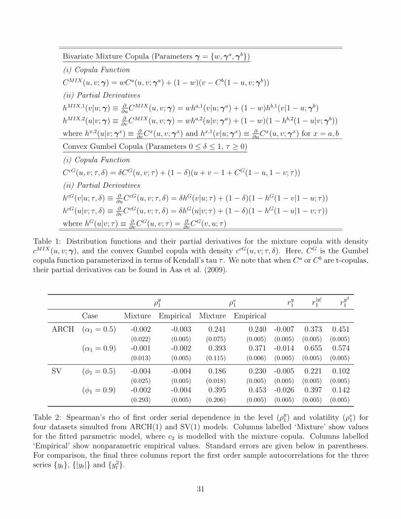
symmetric copula of Oh and Patton (2016b) in the bivariate case. Table 1 gives the copula functions

CMIX , CcG for both the mixture and convex Gumbel copulas.

To show that CMIX can reproduce the features exhibited by the empirical copulas in Figure 2(a–

d), we fit it (with t copula components) to the same four copula datasets. The parameters γ are

estimated by maximizing the copula density at Equation (3), which is the likelihood conditional on

the copula data (the point estimates are reported in the Online Appendix). Figure 2(e–h) plots

c2 for the four estimated copulas, and in each case the mixture copula reproduces the shape of

6

the corresponding empirical copula well. To show the mixture copulas also replicate the quantile

dependence, we compute the quantile dependence coefficients λlow(α) = P (ut < α|ut−1 < α) and

λup(α) = P (ut > α|ut−1 > α), for both the fitted mixture copulas and the empirical copulas. Figure 3

plots these coefficients against α, where λlow(α) is plotted for 0 < α < 0.5, and λup(α) for 0.5 < α < 1.

The coefficients of the mixture and empirical copulas are very close. Figure 2 in the Online Appendix

shows that the same is true for the quantile dependence coefficients in the off-diagonal quadrants.

For Markov processes of order p > 1, we follow Smith et al. (2010) and use a drawable vine (or ‘D-

vine’). A vine copula density is equal to the product of the densities of a sequence of bivariate copula

components, called ‘pair-copulas’ (Aas et al. , 2009). In a general D-vine there are T (T−1)/2 of these,

although in our stationary time series case there are only p unique pair-copulas and a single ordering

of the variables (i.e. the time order). To define the D-vine, for s < t denote ut|s = F (ut|us, . . . , ut−1),

us|t = F (us|us+1, . . . , ut) and ut|t = ut = Ft(yt). Then, as shown in Appendix A, the D-vine copula

density is

cDV (u) =T∏t=2

f(ut|umax(1,t−p), . . . , ut−1)

=T∏t=2

min(t−1,p)∏k=1

ck+1

(ut−k|t−1, ut|t−k+1;γk+1

). (5)

When p = 1, cDV is equal to the density at Equation (3). Each pair-copula density ck+1 has a param-

eter vector γk+1, which we denote explicitly. When k > 1, ck+1 captures dependence between yt−k

and yt, conditional on the intervening observations (yt−k+1, . . . , yt−1). When the series is strongly sta-

tionary, the bivariate distribution of yt−k, yt|yt−k+1, . . . , yt−1 does not vary with t, so that neither does

the pair-copula density ck+1 nor the parameters γk+1. Throughout this paper we use mixture copulas

with densities given at Equation (4) for each of the pair-copula components c2, . . . , cp+1. Therefore,

each pair-copula ck+1 has parameter vector γk+1 = {wk+1,γak+1,γ

bk+1}, and the vine copula density

cDV has parameters γ = {γ2, . . . ,γp+1}. Last, the pair-copula arguments ut|s, us|t are computed from

u using the efficient algorithm in Appendix C.1.

We show how the vine copula can replicate the serial dependence characteristics of three ARCH(3)

7

models in the Online Appendix.

2.2 Measuring Persistence in Volatility

We measure serial dependence in the series values using the bivariate marginal copulas

c(ut−k, ut) =

∫cDV (u)duj /∈{t−k,t} ,

for k ≥ 1. When k = 1, the marginal copula is simply the pair-copula c2(ut−1, ut;γ2). When k > 1, the

marginal copulas are unavailable in closed form, but can be computed via simulation from the D-vine;

see Smith et al. (2010) for details on how to simulate from a vine copula. However, popular pairwise

dependence measures computed from these marginal copulas do not measure volatility persistence.

For example, for the ARCH and SV processes above, both Spearman’s rho and Kendall’s tau of c2

are exactly zero.

We therefore propose new measures of volatility persistence. These are computed from the bivari-

ate copulas of (vt−k, vt), for k ≥ 1, where vt = V (yt−E(yt)) is a transformation of the mean-corrected

time series values. The smooth transformation V : R→ R+ is defined so that:

(i) V (a) = V (−a) > 0, and V (0) = 0 (symmetry around zero), and

(ii) ddaV (a) > 0 if a > 0, and d

daV (a) < 0 if a < 0 .

Examples include V (a) = |a| and V (a) = a2, and we label the copula of (vt−k, vt) a ‘volatility copula’.

Measures of dependence computed from this volatility copula are pairwise measures of volatility

persistence in the time series at lag k. The copula functions and densities of these transformed time

series values are given by the following theorem.

Theorem 1 For s < t, let ys, yt be time series observations with marginal distribution functions

Fs, Ft, marginal means µs, µt, bivariate marginal copula function C and density c. Then the copula

function of the transformed values vs = V (ys − µs), vt = V (yt − µt) is

CV (us, ut) =2∑i=1

2∑j=1

(−1)i(−1)jC(Fs(µs + (−1)iG(F−1Vs

(us))), Ft(µt + (−1)jG(F−1Vt

(ut)))), (6)

8

with corresponding density

cV (us, ut) =

∑2i=1

∑2j=1 f

(µs + (−1)iG(F−1Vs

(us)), µt + (−1)jG(F−1Vt(ut))

)G′(F−1Vs

(us))G′(F−1Vt

(ut))

fVs(F−1Vs

(us))fVt(F−1Vt

(ut)) ,

where

FVj(vj) = Fj(G(vj) + µj)− Fj(−G(vj) + µj) ,

fVj(vj) = (fj(G(vj) + µj) + fj(−G(vj) + µj))G′ (vj) ,

are the marginal distribution and density functions of vj, for j ∈ {s, t}, uj = FVj(V (yj − µj)), and

G is a differentiable function such that G(V (a)) = |a| for any a ∈ R.

Proof: See Appendix B.1.

Note that in Theorem 1 above we do not index C, CV , c and cV by s, t to aid readability.

We make a number of observations about the expressions for CV and cV in Theorem 1. First,

they do not vary with specific choice of transformation V . Consequently, measures of dependence

computed from this copula are also invariant with respect to V , and in this way are general measures

of volatility persistence. Second, they can be computed analytically, except for the inversion of

FVj , which is numerical. Third, they apply equally to stationary or non-stationary time series {yt}.

However, in the former case, CV and cV can be further simplified because the margin is time invariant,

so that Fs = Ft for all s, t. Last, the expressions are not only a function of the marginal copula of

(ys, yt), but also of the margins Fs, Ft. The implication for applied modeling is that the choice of

copula at Equation (1) does not solely determine the form and degree of persistence in the volatility

of the series {yt}.

When both Fs and Ft are symmetric, the expressions for CV and cV are simplified as below.

Lemma 1 If Fs and Ft are both symmetric, then

CV (us, ut) =2∑i=1

2∑j=1

(−1)i(−1)jC

(1 + (−1)ius

2,1 + (−1)jut

2

), and

9

cV (us, ut) =1

4

2∑i=1

2∑j=1

c

(1 + (−1)ius

2,1 + (−1)jut

2

).

Proof: See Appendix B.2

In Lemma 1, the expressions for CV and cV do not involve Fs or Ft so that, in this special case only,

the persistence in the volatility of the series is unaffected by the choice of marginal distributions.

When s = t − k, measures of dependence computed from CV are persistence metrics for the

volatility at lag k ≥ 1. For example, Spearman’s rho is

ρvt−k,t = 12

∫ ∫CV (ut−k, ut)dutdut−k − 3 = 12E(ut−kut)− 3 . (7)

For the D-vine, when k = 1 the marginal copula for (yt−1, yt) is the pair-copula with density

c2(ut−1, ut;γ2). From this, CV can be computed using Theorem 1, and ρvt−1,t at Equation (7) eval-

uated by bivariate numerical integration. However, when k > 1, the marginal copula for (yt−k, yt)

is unavailable in closed form, and ρvt−k,t needs to be evaluated via Monte Carlo simulation. We note

that because our time series model is stationary, it is straightforward to show that ρvt−k,t does not

vary with t, so that we simply denote it as ρvk. Last, other measures of dependence can be computed

from CV similarly.

To highlight the coherence of this measure of persistence in volatility, we compute ρv1 for the four

heteroskedastic time series used to fit the copulas depicted in Figure 2. Table 2 reports these values,

along with Spearman’s rho between (yt−1, yt), which we denote as ρy1. Both metrics are computed

using numerical integration for the fitted mixture copulas. For comparison, we also compute equiva-

lent nonparametric estimates of ρv1 and ρy1 directly from the time series {yt} and {vt}. We make three

observations. First, ρy1 is close to zero throughout, and is an inadequate measure of serial dependence

for these heteroskedastic time series. Second, ρv1 is positive throughout, and increases as the parame-

ters α1 and φ1 of the ARCH(1) and SV(1) models increase. Third, the values for ρy1 and ρv1 computed

using the fitted parametric mixture copula are similar to those computed empirically. This is further

evidence that the mixture copula is an adequate parametric model of serial dependence for the het-

eroskedastic series. For further comparison, we also report the first order linear autocorrelations of

10

the series, the absolute values |yt|, and the squared values y2t . These are consistent with those from

the mixture copula model, although the autocorrelations of the squared and absolute values differ–

whereas ρv1 is invariant to the form of transformation V .

2.3 Modeling USD/AUD Exchange Rate

2.3.1 First order copula model

To illustrate the advantages of our time series copula model, we employ it to model daily returns on

the USD/AUD exchange rate from 2 Jan 2001 until 7 Aug 2015, sourced from the Federal Reserve

Economic Data (FRED) database. The series exhibits strong heteroskedasticity, along with an asym-

metric and heavy-tailed marginal distribution. Figure 4 plots a histogram of the T = 3669 returns,

which have skew of −0.654 and kurtosis of 15.15. Also plotted are the margins of GARCH(1,1),

EGARCH(1,1) and GARCH-t(1,1) models fit to this data, computed by simulation. These mod-

els are widely used for such data (Hansen and Lunde, 2005), yet have margins that are necessarily

symmetric and inaccurate. In contrast, we model the margin nonparametrically using the adaptive

kernel density estimator of Shimazaki and Shinomoto (2010)— also plotted on Figure 4— from which

the copula data are computed. The use of a nonparametric time invariant margin, combined with a

parametric copula, is also advocated by Chen and Fan (2006) and Chen et al. (2009) for stationary

Markov series. We employ the first order time series copula at Equation (3), with the mixture copula

for c2, where ca, cb are the densities of bivariate t copulas, so that there are 5 copula parameters.

The resulting copula model allows for heteroskedastic serial dependence, but with a margin that is

consistent with that observed empirically.

We estimate the copula parameters using both MLE and Bayesian posterior inference. For the

latter, flat or uninformative proper priors are used for the copula parameters, and computation is by

Markov chain Monte Carlo (MCMC), where the parameters were generated as a block using adaptive

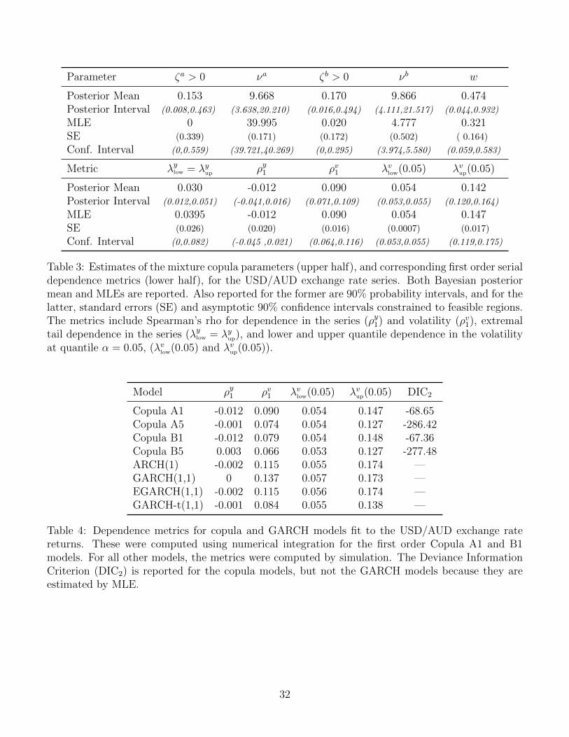
random walk Metropolis-Hastings (Roberts and Rosenthal, 2009). Table 3 reports the point estimates

for both the copula parameters and serial dependence metrics. Also reported are 90% confidence

intervals for the MLE, along with the 90% posterior probability intervals. We make the following

observations. First, while the confidence and posterior intervals are wide for the parameters, those

11

for the dependence metrics are not. This is common for copulas with multiple parameters, where a

wide range of parameter values can correspond to similar copula functions and dependence values.

Second, the posterior mean and MLE for the dependence metrics are almost identical. Third, return

values exhibit negligible first order serial dependence (ρy1), but have positive first order extremal tail

dependence (λylow = limα→0 Pr(ut < α|ut−1 < α)). Last, our proposed measure of first order volatility

persistence (ρv1) is positive, as are the corresponding quantile dependence metrics (λvlow(α) = Pr(ut <

α|ut−1 < α) and λvup(α) = Pr(ut > 1 − α|ut−1 > 1 − α)) computed from the volatility copula in

Theorem 1.

Finally, Figure 5 plots the fitted copula density in panel (a). For comparison, also plotted in

panel (b) is the density of a first order copula model fitted to the same data, but where cMIX has

convex Gumbel components. Both densities are very similar and have the ‘cross shape’ that is

indicative of serial dependence in heteroskedastic series.

2.3.2 Validation study

Based on the USD/AUD exchange rate data, we undertake a validation study. We fit four time series

copulas of the form at Equation (5) to the copula data, as follows:

Copula A1: An order p = 1 D-vine with t-copula based mixture components.

Copula A5: An order p = 5 D-vine with t-copula based mixture components.

Copula B1: An order p = 1 D-vine with convex Gumbel based mixture components.

Copula B5: An order p = 5 D-vine with convex Gumbel based mixture components.

Copula A1 is the first order model in Section 2.3, to which we add a higher order D-vine with

p = 5 and component pair-copulas of the same form. Copulas B1 and B5 are also D-vines with pair-

copula densities given by cMIX , each with component densities ca and cb that are convex Gumbel

densities discussed previously. Note that both Copulas A1 and B1 are five parameter copulas, whereas

Copulas A5 and B5 are parsimonious D-vines with a total of 5×5 = 25 parameters each. The posterior

of the copula models are obtained using MCMC, where the parameters of each pair-copula were

12

generated as a block using adaptive random walk Metropolis-Hastings, and with blocks generated in

random order. Table 4 reports the deviance information criteria (DIC) for each copula model. This

is computed conditional on the same copula data, and is DIC2 of Celeux et al. (2006). Lower DIC

values are preferred, so that longer lag lengths dominate, with Copula A5 optimal by this measure.

The ARCH(1), GARCH(1,1), GARCH-t(1,1) and EGARCH(1,1) models, estimated using MLE,

are used as benchmarks. Table 4 reports the four (first order) serial dependence metrics. As expected,

for all models, serial dependence in the returns (ρy1) is close to zero, and volatility persistence (ρv1)

is positive. In each model, the first order (k = 1) volatility copula exhibits asymmetric and positive

quantile dependence (λvup(0.05) > λvlow(0.05) > 0), which is something that we repeatedly observe

with heteroskedastic series. Interestingly, the metrics from the copula models are close to those of

the GARCH-t(1,1) model, which is widely considered the most accurate of the benchmark models

for daily exchange rate returns (Baillie and Bollerslev, 2002).

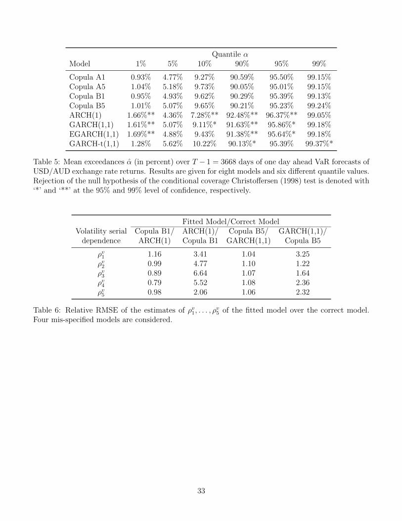
To judge the quality of the fitted models, we examine one day ahead VaR coverage as follows.

For each fitted model, the 1-step ahead predictive distributions Ft|t−1(yt) are computed for days

t = 2, . . . , T . From these we compute V aRt|t−1(α) = F−1t|t−1(α), for 0 < α < 1, along with the mean

number of exceedences during the T − 1 = 3668 days, defined as α = 1T−1

∑Tt=2 1(yt < V aRt|t−1(α)).

Table 5 reports α for α ∈ {0.01, 0.05, 0.1, 0.9, 0.95, 0.99}, and shows that the copula models have

accurate coverage. Figure 6 plots α from the Copula B5 and four GARCH models against α, for

values 0.01 < α < 0.1 in panel (a), and 0.9 < α < 0.99 in panel (b). Deviations from the black 45

degree line indicate inaccurate VaR coverage, and it can be seen that the copula model dominates

the GARCH models in both tails– particularly those with Gaussian innovations. We note that the

predictive distributions of the GARCH models are necessarily Gaussian or t, whereas those from the

copula models are not.

Last, in Table 5 we also report the results of the Christoffersen (1998) test of correct conditional

coverage for all quantiles and models. This test assesses jointly whether the empirical coverage equates

to the corresponding theoretical value and whether the exceedences are serially independent. Models

that produce forecasts that fail to reject the conditional coverage test are deemed to perform well in

13

predicting VaR. The test results suggest all four copula models dominate the GARCH benchmarks.

2.4 Simulation Study

To illustrate the robustness of the time series copula to model misspecification we undertake a small

simulation study based on the AUD/USD exchange rate data. One hundred datasets, each of length

T = 3669, were simulated from the fitted ARCH(1), Copula B1, GARCH(1,1) and Copula B5 models

in Section 2.3.2 above. For each model and dataset we fit both the correct and one incorrect model

(listed in Table 6), giving eight fitted models in total.

To measure the accuracy of the estimated volatility dependence, we compute ρv1, . . . , ρv5 from the

fitted models. These coefficients are computed by simulating series of length 1 million from the

models, and then computing the sample Spearman’s rho of V (yt) and V (yt−k) for k = 1, . . . , 5. We

repeat this for all 100 datasets and compute the root mean squared error (RMSE) for each coefficient

and fitted model. Here, the true value of ρvk can be computed accurately via simulation from the

true model as well. Table 6 reports the ratio of the RMSE values of the misspecified models, relative

to that obtained by fitting the correct model. Greater relative RMSE values indicate that the fitted

misspecified model does not capture the volatility serial dependence well. The results indicate that

the two copula models reproduce the volatility serial dependence structure of the GARCH models

well, although the converse is not true. For example, for ρv1 the relative RMSEs of incorrectly fitting

the Copula B1 and B5 models are only 1.16 and 1.04; yet the relative RMSEs are 3.41 and 3.25 when

incorrectly fitting the ARCH(1) and GARCH(1,1) models.

3 Multivariate Heteroskedastic Time Series

3.1 Copula Model

Copulas can also be used to model dependence in multivariate time series. The copula model for the

T observations y = (y′1, . . . ,y′T )′ of a vector yt = (y1,t, . . . , ym,t)

′ of m continuous values has density

f(y) = c(u)T∏t=1

m∏j=1

fj,t(yj,t) , (8)

14

where u = (u′1, . . . ,u′T )′, ut = (u1,t, . . . , um,t)

′, uj,t = Fj,t(yj,t), Fj,t is the marginal distribution

function of yj,t, and fj,t(yj,t) = ddyj,t

Fj,t(yj,t). The copula density in Equation (8) is of dimension

mT , and captures both serial and cross-sectional dependence in the series jointly. Selection of an

appropriate high-dimensional copula is the main challenge in constructing the model.

Biller and Nelson (2003), Biller (2009) and Smith and Vahey (2016) all use Gaussian copulas, with

parameter matrix equal to the correlation matrix of a stationary vector autoregression. However,

just as in the univariate case, the Gaussian copula is unable to capture the volatility persistence

exhibited by heteroskedastic time series. As an alternative, Beare and Seo (2015), Brechmann and

Czado (2015) and Smith (2015) all suggest using vine copulas for (strongly) stationary series. We

follow these authors and employ a D-vine, with pair-copula components of the form at Equation (4)

to capture heteroskedasticity. We outline this below, although refer to Smith (2015) for further

details on the specification of the vine and its time series properties.

When the multivariate series is (strongly) stationary and Markov of lag p, the D-vine copula

density can be written as

c(u) = K0(u1)T∏t=2

K0(ut)

min(t−1,p)∏k=1

Kk(ut−k, . . . ,ut)

. (9)

The functionals K0, . . . , Kp are each products of blocks of pair-copula densities, and do not vary with

t for stationary series. They are defined as

Kk (ut−k, . . . ,ut) =

∏m

l1=1

∏l1−1l2=1 c

(0)l2,l1

(uj|i−1, ui|j+1;γ

(0)l2,l1

)if k = 0∏m

l1=1

∏ml2=1 c

(k)l2,l1

(uj|i−1, ui|j+1;γ

(k)l2,l1

)if 1 ≤ k ≤ p ,

where c(k)l2,l1

is a bivariate pair-copula density with parameters γ(k)l2,l1

. When k = 0, there are m(m−1)/2

of these associated with K0, and they collectively capture cross-sectional dependence between the m

variables. For example, if they were each equal to the bivariate independence copula with density

c(0)l2,l1

= 1, then K0 = 1 and the variables would be independent at any given point in time. When

15

k > p, there are m2 pair-copulas associated with block Kk that capture serial dependence at lag k.

In total, there are p(m2) +m(m− 1)/2 unique pair-copulas, which is much less than the Tm(Tm−

1)/2 in an unconstrained D-vine. The indices of the pair-copula arguments are i = l1 + m(t − 1)

and j = l2 + m(t − k − 1), and the argument values themselves ui|j, uj|i are computed using the

algorithm in Appendix C.2. Last, we note that if m = 1, then K0 = 1, i = t, j = t − k and Kk =

c(k)1,1(ut−k|t−1, ut|t−k+1), so that with the notation ck+1 ≡ c

(k)1,1, the copula densities at Equations (5)

and (9) are the same.

3.2 Estimation, Serial Dependence and Volatility Dependence

Estimation is similar to the univariate case. The marginal distribution of each variable is estimated

nonparametrically using adaptive kernel density estimation, from which the copula data are con-

structed. Equation (9) gives the likelihood, conditional on the copula data. It can be difficult to

maximize for higher values of m and p, so that we follow Min and Czado (2010) and Smith et al.

(2010) and use MCMC to evaluate the posterior distribution. In the sampling scheme, the parameter

vector of each unique pair-copula is generated jointly, conditional on the parameters of the other pair-

copulas. To do so, a Metropolis-Hastings step with an adaptive multivariate random walk Gaussian

proposal (Roberts and Rosenthal, 2009) is used. Key to implementation is the efficient computation

of the likelihood, as outlined in Appendix C.2.

Serial dependence in the series is summarized using measures of dependence between pairs

(yi,t−k, yj,t). These can be arranged into a (m × m) matrix for any given value of k ≥ 0. Be-

cause the bivariate marginal copula between each pair is unavailable in closed form, we compute the

metrics via Monte Carlo simulation from the vine copula. This can be undertaken efficiently using

Algorithm 2 of Smith (2015). For example, pairwise Spearman’s rho can be computed as

ρyi,j,k = 12E(ui,t−kuj,t)− 3 ≈

(12

L

L∑l=1

u[l]i,1u

[l]j,k+1

)− 3 ,

where {u[l]i,t; i = 1, . . . ,m, t = 1, . . . , k+ 1} is an iterate from the joint distribution of {u1, . . . ,uk+1},

for l = 1, . . . , L. Then the matrix P yk = {ρyi,j,k}1≤i≤m;1≤j≤m is a measure of overall kth order serial

16

dependence in the multivariate time series.

Similar dependence measures can be computed for the pair of volatility proxies (vi,t−k, vj,t), where

vi,t = V (yi,t − µi,t), µi,t = E(yi,t), and V is the function defined in Section 2.2. While Theorem 1

is directly applicable here, the bivariate copula of (vi,t−k, vj,t) cannot be computed in closed form

because the underlying marginal copula of (yi,t−k, yj,t) cannot either. Therefore, we again compute

the dependence measures via Monte Carlo simulation, where iterates of the volatility proxies can

be computed directly from those generated for the series. If Spearman’s rho of the pair (vi,t−k, vj,t)

is denoted as ρvi,j,k, then these values can be arranged into matrices P vk = {ρvi,j,k}1≤i≤m;1≤j≤m, for

a given lag k ≥ 0. The matrix P v0 measures cross-sectional dependence in volatility at a point

in time, with the off-diagonal elements measuring volatility co-movement. For k ≥ 1 the leading

diagonal elements of P vk are measures of own-series volatility persistence, whereas the off-diagonals

are measures of volatility spillover. Volatility co-movement and spillover are widely documented in

daily asset and exchange rate returns (Hamao et al., 1990, Baillie and Bollerslev, 1991), although

multivariate GARCH models usually measure these through conditional moments, not marginally as

we propose here.

3.3 Multivariate Model of Exchange Rates

We extend the analysis of the USD/AUD exchange rate in Section 2.3 to include the USD/EUR

and USD/JPY rates, which are the two most traded currency pairs. As before, daily returns were

computed using rates sourced from the FRED database which are synchronized to New York closing

time. The USD/EUR and USD/JPY returns are both asymmetric (with skew 0.044 and 0.278) and

fat-tailed (with kurtosis 5.23 and 7.22). Each margin is modeled nonparametrically using an adaptive

kernel density estimator; see Figure 3 of the Online Appendix. The D-vine copula at Equation (9)

with p = 1 is used to capture both cross-sectional and serial dependence simultaneously, with pair-

copula densities given by cMIX at Equation (4). For the components of the mixture copula we use

either all t-copulas, or all convex Gumbels, resulting in two D-vines which we label ‘Copula A’ and

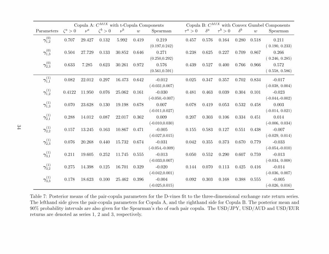
‘Copula B’, respectively. Both have a total of 12 × 5 = 60 parameters, and their posterior mean

estimates are reported in Table 7.

17

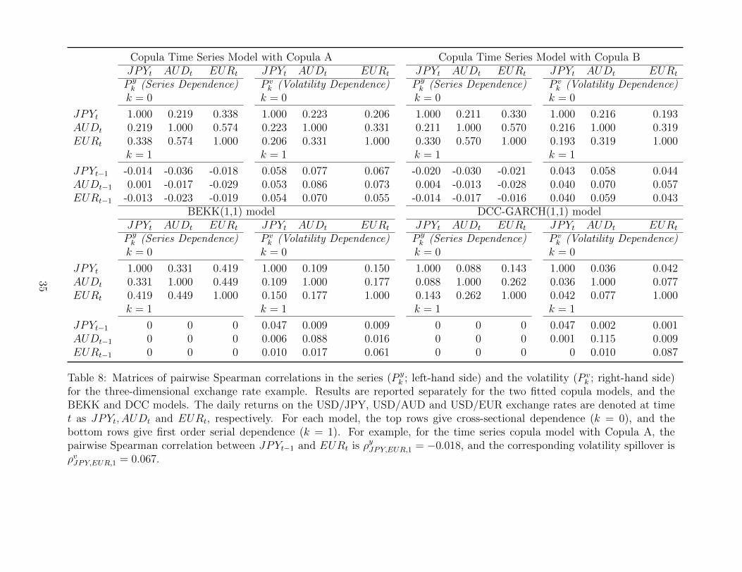
To summarize serial dependence in both the series and its volatility, the top of Table 8 reports

the posterior mean estimates of the matrices P yk and P v

k of pairwise marginal Spearman’s rho. Re-

sults are reported for contemporaneous (k = 0) and first order serial (k = 1) dependence. Results

are very similar for both Copulas A and B, and we make a number of observations. First, cross-

sectional dependence in the returns (P y0 ) is positive throughout, with that between the USD/AUD

and USD/EUR currency pairs being the highest. Second, there is negligible first order serial depen-

dence in the returns (P y1 ). Third, there is co-movement in the volatility of the three series, with

positive values on the off-diagonal of P v0 . Fourth, there is volatility persistence in each series, with

positive values along the leading diagonal of P v1 . Last, there are positive volatility spillovers between

series, as measured by the off-diagonal elements of P v1 . All five features are consistent with previous

studies of daily exchange rate returns (Baillie and Bollerslev, 2002, Nakatani and Terasvirta, 2009).

We compare the dependence matrices with those computed from two trivariate GARCH models.

These are the DCC-GARCH(1,1) (Engle, 2002) and BEKK(1,1) (Engle and Kroner, 1995) models.

The diagonal form of the BEKK model is used because the likelihood for the full form is not log-

concave for this series, which is a well-known problem. Table 8 also reports the dependence matrices

for these two models, which are computed via simulation, and we make four observations. First, all

models have positive return co-movements P y0 , but are lowest for the DCC-GARCH(1,1). Second,

volatility co-movements P v0 are also positive for all models, but are stronger for the copula models.

Third, volatility persistence, given by the leading diagonal of P v1 , is similar in size for all four models.

Last, the major difference is that the off-diagonals of P v1 are positive for the copula models, but

almost zero for the two GARCH models. Thus, first order volatility spillovers are indicated by the

copula model, but are not by the multivariate GARCH models.

We extend the validation study to include these multivariate models, plus the BEKK(1,0) model.

We construct the one-day-ahead predictive distributions for the three returns series and the return

on an equally-weighted currency portfolio. As in Section 2.3.2 we compute the mean number of

exceedances α, and plots of these against the quantile α (given in the Online Appendix) suggest the

copula models have more accurate VaR coverage than the multivariate GARCH models. For the

18

equally-weighted currency portfolio, Table 9 reports exceedances for all five models and the results

of the Christoffersen tests at six quantiles. As in the univariate case, the copula models dominate

the multivariate GARCH models.

To illustrate the difference in density forecasts, we plot these for the USD/JPY return on three

days in Figure 7. These are the days with the lowest and highest returns during the last 18 months in

the data, along with the day with return closest to zero. Panels (a–c) plot the densities, while panels

(d–f) plot their logarithm to better visualize the tails. For simplicity, we only plot the densities

for Copula A, although for Copula B are similar. Note that the multivariate GARCH models are

conditionally Gaussian, so that their predictive distributions are also. In contrast, the copula forecast

densities in panels (a–c) are asymmetric, with skew coefficients of 0.113, 0.473 and 0.316, respectively.

Panels (d–f) show that the density forecasts from the copula model also have heavy tails, with a

kurtosis of 5.78, 7.39 and 6.44, respectively. Clearly, the nonparametric margins combined with the

copula function, translate into non-Gaussian predictive distributions.

4 Discussion

Time series copula models are very general, in that all time series models have a copula specification.

For example, Smith and Maneesoonthorn (2016) show how to compute the copula of a nonlinear state

space model numerically. However, for many existing time series models — including popular models

for heteroskedastic data — the time series copula cannot be written in closed form. Our approach

is therefore an alternative copula specification to capture serial dependence for heteroskedastic data.

For stationary first order Markov series the bivariate copula density has mass concentrated along

the two diagonals of the unit cube, which mirrors that found empirically for two popular existing

heteroskedastic models. It is extended to higher Markov orders and multivariate time series using D-

vines. An important observation is that these vines are highly parsimonious, with densities that can

be evaluated using O(T ) parallel algorithms. This enables the copula models to be readily estimated

for the longer series encountered in practice.

The main theoretical result is the derivation of the bivariate copula of a volatility proxy at two time

19

points. We find that the copula does not depend on the specific transformation V used in Section 2.2.

For example, it is the same if the volatility proxy is either vt = |yt−E(yt)| or vt = (yt−E(yt))2. The

copula fully characterizes the (unconditional) dependence between vt and vt−k at a given lag k ≥ 1.

While it is a function of the time series copula, it is also a function of the marginal distribution

of the data whenever that margin is asymmetric. This has an important implication for applied

modeling: while the choice of C in Equation (1) completely determines the serial dependence of the

series, it does not always do so for volatility. We show how dependence metrics can be computed

from the volatility copulas, which provide measures of volatility persistence, along with co-movement

and spillover for multivariate series. These can be computed by simulation for any stationary time

series, not just the copula model proposed here. They can be used to compare the degree of volatility

dependence arising from different nonlinear time series models, as in Tables 4 and 8.

A major advantage of copula models is the simplicity with which they incorporate complex mar-

gins; for example, the exchange rate returns series exhibit asymmetry and heavy tails. As noted

by Chen and Fan (2006) and others, these can be accurately captured using nonparametric methods,

and we show in Figure 7 that these affect the forecast densities substantitally. In comparison, most

existing time series models are conditionally Gaussian or t distributed, and density forecasts are

also; e.g. see Clark and Ravazzolo (2015). Moreover, the marginal distributions are often poorly

calibrated, as illustrated in Figure 4. Ultimately, the VaR forecasts from the copula model are more

accurate. We illustrate this using daily exchange rate returns with GARCH benchmark models in

the univariate case, and BEKK and DCC benchmark models in the multivariate case. In the latter,

our copula model also dominates the multivariate GARCH models for a portfolio of the three rates,

indicating that the copula also captures the cross-sectional dependence accurately.

20

Appendix A D-vine Copula Density

In this appendix we outline the derivation of the D-vine copula density at Equation (5). The copula

density of a Markov p process can written as

cDV (u) =T∏t=2

f(ut|umax(1,t−p), . . . , ut−1) ,

where f(u1) = 1 because the marginal distribution of u1 is uniform on [0, 1]. For t− p ≤ s < t, there

always exists a density ct,s on [0, 1]2 such that

f(ut, us|ut−1, . . . , us+1) = f(ut|ut−1, . . . , us+1)f(us|ut−1, . . . , us+1)

× ct,s (F (us|ut−1, . . . , us+1), F (ut|ut−1, . . . , us+1);ut−1, . . . , us+1) ,

which is the theorem of Sklar applied conditional on ut−1, . . . , us+1. In a vine copula, ct,s is a bivariate

pair-copula density, and it is simplified by dropping dependence on (ut−1, . . . , us+1). The pair-copula

captures the dependence between yt and ys, conditional on the intervening observations. Denoting

us|t−1 = F (us|ut−1, . . . , us+1) and ut|s+1 = F (ut|ut−1, . . . , us+1), the above gives f(ut|ut−1, . . . , us) =

ct,s(us|t−1, ut|s+1)f(ut|ut−1, . . . , us+1). Repeated application of the above with s = max(1, t−p), . . . , t−

1 gives

f(ut|umax(1,t−p), . . . , ut−1) =t−1∏

s=max(1,t−p)

ct,s(us|t−1, ut|s+1)

=

min(p,t−1)∏k=1

ct,t−k(ut−k|t−1, ut|t−k+1) ,

where we set s = t−k. If the series is stationary, it is straightforward — for example, see Smith (2015)

— to show that the pair-copulas ct,t−k are invariant with respect to t, so that we can write ct,t−k = ck+1

throughout, resulting in Equation (5).

Last, we note that compared to Equation (2.4) of Smith et al. (2010), the order of the two argu-

ments of each pair-copula is switched. While this is unimportant when the pair-copula is symmetric,

21

it is when the pair-copula is asymmetric, as with the mixture copula cMIX here. It is particularly

important to keep note of the order of the arguments of the pair-copulas when implementing the

algorithms in Appendix C.

Appendix B Copula of Transformed Variables

Consider two continuous random variables Y1 and Y2, with joint distribution function F , bivariate

copula function C and density c, and marginal distribution functions F1 and F2, respectively. (In

Theorem 1 and Lemma 1, these random variables correspond to the time series at times s and t,

respectively.) In this appendix we derive the bivariate copula function CV of V1 = V (Y1 − µ1) and

V2 = V (Y2 − µ2), where V : R → R+ is the transformation defined in Section 2.2, µ1 = E(Y1) and

µ2 = E(Y2). We show that, in general, CV is a function of both C, and also the marginals F1 and

F2. We also derive the copula density cV of V1 and V2. We consider separately the special case where

both Y1 and Y2 are strictly symmetrically distributed.

B.1 General Marginals Case

Let G(V (a)) = |a| for any a ∈ R, and G(.) is a differentiable function function, where G : R+ → R+.

Recognizing that G(vj) = G(V (yj − µj)) = |yj − µj|, the values of vj can be mapped to yj (in a

one to two mapping), by the identity yj = (−1)iG(vj) + µj, for i ∈ {1, 2}. Since this mapping is

deterministic, through the G function, the joint distribution of (V1, V2) can be derived from the joint

distribution of (Y1, Y2):

FV (v1, v2) = Pr (−G(v1) < Y1 − µ1 < G(v1),−G(v2) < Y2 − µ2 < G(v2))

=2∑i=1

2∑j=1

(−1)i(−1)jF((−1)iG(v1) + µ1, (−1)jG(v2) + µ2

).

Further, by Sklar’s Theorem, F (y1, y2) = C(F1(y1), F2(y2)), so FV (v1, v2) can be written as a function

of C(F1(y1), F2(y2)) as

FV (v1, v2) =2∑i=1

2∑j=1

(−1)i(−1)jC(F1

((−1)iG(v1) + µ1

), F2

((−1)jG(v2) + µ2

)).

22

With the marginal distribution function of Vj denoted by FVj and the corresponding copula datum

uj = FVj(vj), inverting Sklar’s theorem yields the copula function

CV (u1, u2) = FV(F−1V1

(u1), F−1V2

(u2))

=2∑i=1

2∑j=1

(−1)i(−1)jC(F1

((−1)iG(F−1V1

(u1)) + µ1

), F2

((−1)jG(F−1V2

(u2)) + µ2

)), (10)

where FVj(vj) = Pr(Vj < vj) = Pr (−G(vj) < Yj − µj < G(vj))

= Fj (G(vj) + µj)− Fj (−Gj(vj) + µj) . (11)

The quantile function F−1Vjcan be obtained by numerically inverting (11) for any given marginal Fj.

The copula density can be obtained by differentiating the copula function in (10):

cV (u1, u2) =∂2

∂u1∂u2CV (u1, u2)

=2∑i=1

2∑j=1

c(F1

(µ1 + (−1)iG(F−1V1

(u1))), F2

(µ2 + (−1)jG(F−1V2

(u2))))f1(µ1 + (−1)iG(F−1V1

(u1)))×

f2(µ2 + (−1)jG(F−1V2

(u2)))G′(F−1V1

(u1))G′(F−1V2

(u2))

fV1(F−1V1

(u1))fV2(F−1V2

(u2))

=

∑2i=1

∑2j=1 f

(µ1 + (−1)iG(F−1V1

(u1)), µ2 + (−1)jG(F−1V2(u2))

)G′(F−1V1

(u1))G′(F−1V2

(u2))

fV1(F−1V1

(u1))fV2(F−1V2

(u2))

with

fVj(vj) =d

dvjFVj(vj) = (fj(G(vj) + µj) + fj(−G(vj) + µj))G

′(vj) .

B.2 Symmetric Marginals Case

In the special case where the marginal distributions F1 and F2 are both symmetric around their

respective means, we have that Fj(−G(vj) + µj) = 1− Fj(G(vj) + µj), for j = {1, 2}. Applying this

23

relation to Equation (11), gives

FVj(vj) = 2Fj(G(vj) + µj)− 1.

By substituting FVj(vj) = uj and vj = F−1Vj(uj), along with simple rearrangements,

G(F−1Vj(uj)) = F−1j

(1 + uj

2

)− µj.

Since the marginal distribution is symmetric around µj, we also have that

−G(F−1Vj(uj)) = F−1j

(1− uj

2

)− µj.

Substituting the simplified expressions for G(F−1Vj(uj)) and −G(F−1Vj

(uj)) into Equation (10) gives

CV (u1, u2) =2∑i=1

2∑j=1

(−1)i(−1)jC

(1 + (−1)iu1

2,1 + (−1)ju2

2

).

Finally, by differentiating the copula distribution above, the copula density is

cV (u1, u2) =2∑i=1

2∑j=1

1

4c

(1 + (−1)iu1

2,1 + (−1)ju2

2

).

Note that the copula function of the transformed variable in this special case, where both margins

are symmetric around µj, does not depend on the form of the marginal distribution Fj.

Appendix C Efficient Likelihood Evaluation

Computing the two D-vine copula densities at Equations (5) and (9) requires efficient evaluation of

the arguments of the pair-copulas. In this appendix we outline algorithms to compute these. The

algorithms are extensions of that orginally proposed by Aas et al. (2009), and further developed

in Smith et al. (2010) and Smith (2015). They differ in three ways: (i) they are re-ordered so that the

computations can be undertaken in parallel; (ii) they exploit the parsimonious structures of the two

24

vine copulas; and (iii) they are based on recursions that account for the pair-copulas being mixtures

of possibly asymmetric copulas.

C.1 Univariate Series

The arguments of the pair-copulas can be computed by exploiting the recursive relationships

ut|s = h1s,t(ut|s+1|us|t−1) , and us|t = h2s,t(us|t−1|ut|s+1) ,

where, for the specific vine in Equation (5), if k = t− s then

h1s,t(v|u) =∂

∂uCk+1(u, v;γk+1) , and h2s,t(u|v) =

∂

∂vCk+1(u, v;γk+1) .

Here, Ck+1(u, v;γk+1) =∫ u0

∫ v0ck+1(u, v;γ)dudv is the pair-copula function for k = 1, 2, . . . , p. We

note that these recursions are more general than those given in Smith et al. (2010). These authors

assume that h1s,t = h2s,t, which is true for the pair-copula types they examine. However, this is not

the case when the pair-copula is the mixture copula with function CMIX , with the partial derivatives

given in Table 1.

The O(T 2) algorithms in Aas et al. (2009) and Smith et al. (2010) compute and store all T (T−1)

values {ut|s, us|t; 1 ≤ t ≤ T, s < t}, which is impractical for high values of T . However, to compute

the likelihood in Equation (5), only the values U = {ut|s, us|t; 1 ≤ t ≤ T,max(1, t− p) ≤ s < t} need

computing and storing. Moreover, we evaluate the elements of U in a different order to allow the

computations to be undertaken in parallel, as follows:

Algorithm 1.

For t = 1, . . . , T :

Step (1). Set ut|t = ut.

For k = 1, . . . , p:

For t = k + 1, . . . , T (compute inner loop in parallel):

Step (2.1). ut|t−k = h1t−k,t(ut|t−k+1|ut−k|t−1)

Step (2.2). ut−k|t = h2t−k,t(ut−k|t−1|ut|t−k+1)

25

Once computed, the elements in U need to be stored efficiently. It is possible to store these in a

(T×T ) matrix, with ut|s stored in element (t, s), and us|t in element (s, t). However, this is prohibitive

for longer time series. Instead, U can be stored efficiently either as a banded matrix with bandwidth

p, or a (T × p× 2) array, with ut|t−k stored as element (t, k, 1), and ut−k|t as element (t, k, 2). We use

the latter approach in our code.

C.2 Multivariate Series

For the vine copula at Equation (9), there is a one-to-one relationship between the indices (s, t, l1, l2),

and those of the pair-copula arguments (i, j). To evaluate these arguments we use the recursive

relationships

ui|j = h1j,i(ui|j+1|uj|i−1) , and uj|i = h2j,i(uj|i−1|ui|j+1) .

The functions are

h1j,i(v|u) =∂

∂uC

(k)l2,l1

(u, v;γ(k)l2,l1

) , and h2j,i(u|v) =∂

∂vC

(k)l2,l1

(u, v;γ(k)l2,l1

) ,

where s = dj/me, t = di/me, k = t − s, l1 = i −m(t − 1), l2 = j −m(s − 1), and the pair-copula

function C(k)l2,l1

(u, v;γ(k)l2,l1

) =∫ u0

∫ v0c(k)l2,l1

(u, v;γ(k)l2,l1

)dudv. As in the univariate case, we employ CMIX

for the pair-copula functions, so that the partial derivatives required to compute h1i,j and h2j,i above

are given in Table 1. Following (Smith, 2015), we note that only the values

U = {ui|j, uj|i; 1 ≤ i ≤ Tm,max (1,m (di/me − 1− p) + 1) ≤ j < i}

are needed to compute the likelihood. These can be computed using the O(pm2T ) algorithm below.

Algorithm 2.

For t = 1, . . . , T , l = 1, . . . ,m:

Step (1.1). Set i = t+ (l − 1)m.

Step (1.2). Set ui|i = ul,t.

26

For r = 1, . . . , (p+ 1)m− 1:

For i = r + 1, . . . ,mT (compute inner loop in parallel):

Step (2.1). Set j = i− r, s = dj/me, t = di/me, k = t− s, l1 = i−m(t−1), l2 = j−m(s−1).

Step (2.2). Compute ui|j = h1j,i(ui|j+1|uj|i−1).

Step (2.3). Compute uj|i = h2j,i(uj|i−1|ui|j+1).

The arguments in U are efficiently stored in a 3-dimensional (Tm× (m(p+ 1)− 1)× 2) array,

with uj|i stored as element (i, i− j, 1), and uj|i as element (i, i− j, 2).

References

Aas, K., Czado, C., Frigessi, A., and Bakken, H. (2009). Pair-copula constructions of multiple

dependence. Insurance: Mathematics and Economics, 44(2):182 – 198.

Almeida, C. and Czado, C. (2012). Efficient Bayesian inference for stochastic time-varying copula

models. Computational Statistics & Data Analysis, 56(6):1511–1527.

Baillie, R. T. and Bollerslev, T. (1991). Intra-day and inter-market volatility in foreign exchange

rates. The Review of Economic Studies, 58(3):565–585.

Baillie, R. T. and Bollerslev, T. (2002). The message in daily exchange rates: a conditional-variance

tale. Journal of Business & Economic Statistics, 20(1):60–68.

Beare, B. K. (2010). Copulas and Temporal Dependence. Econometrica, 78(1):395–410.

Beare, B. K. (2012). Archimedean copulas and temporal dependence. Econometric Theory,

28(06):1165–1185.

Beare, B. K. and Seo, J. (2015). Vine copula specifications for stationary multivariate Markov chains.

Journal of Time Series Analysis, 36(2):228–246.

Biller, B. (2009). Copula-based multivariate input models for stochastic simulation. Operations

Research, 57(4):878–892.

Biller, B. and Nelson, B. (2003). Modeling and generating multivariate time-series input processes

using a vector autoregressive technique. ACM Transactions on Modeling and Computer Simulation,

13(3):1049–3301.

27

Boothe, P. and Glassman, D. (1987). The statistical distribution of exchange rates: empirical evidence

and economic implications. Journal of International Economics, 22(3):297–319.

Brechmann, E. C. and Czado, C. (2015). COPAR– multivariate time series modeling using the copula

autoregressive model. Applied Stochastic Models in Business and Industry, 31(4):495–514.

Brockwell, P. J. and Davis, R. A. (1991). Time Series : Theory and Methods. Springer Series in

Statistics. Springer, New York (N.Y.).

Celeux, G., Forbes, F., Robert, C. P., and Titterington, D. M. (2006). Deviance information criteria

for missing data models. Bayesian analysis, 1(4):651–673.

Chen, X. and Fan, Y. (2006). Estimation of copula-based semiparametric time series models. Journal

of Econometrics, 130(2):307–335.

Chen, X., Wu, W. B., and Yi, Y. (2009). Efficient Estimation of Copula-based Semiparametric

Markov Models. Annals of statistics, 37(6B):4214–4253.

Christoffersen, P. F. (1998). Evaluating interval forecasts. International Economic Review, 39:841–

862.

Clark, T. E. and Ravazzolo, F. (2015). Macroeconomic forecasting performance under alternative

specifications of time-varying volatility. Journal of Applied Econometrics, 30(4):551–575.

Creal, D. D. and Tsay, R. S. (2015). High dimensional dynamic stochastic copula models. Journal

of Econometrics, 189(2):335–345.

Darsow, W. F., Nguyen, B., and Olsen, E. T. (1992). Copulas and Markov processes. Illinois Journal

of Mathematics, 36(4):600–642.

De Lira Salvatierra, I. and Patton, A. J. (2015). Dynamic copula models and high frequency data.

Journal of Empirical Finance, 30:120–135.

Demarta, S. and McNeil, A. J. (2005). The t copula and related copulas. International Statistical

Review/Revue Internationale de Statistique, pages 111–129.

Domma, F., Giordano, S., and Perri, P. F. (2009). Statistical modeling of temporal dependence in

financial data via a copula function. Communications in Statistics - Simulation and Computation,

38(4):703–728.

Engle, R. (2002). Dynamic conditional correlation: A simple class of multivariate generalized au-

toregressive conditional heteroskedasticity models. Journal of Business & Economic Statistics,

20(3):339–350.

28

Engle, R. F. and Kroner, K. F. (1995). Multivariate simultaneous generalized ARCH. Econometric

Theory, 11(01):122–150.

Fortin, I. and Kuzmics, C. (2002). Tail-dependence in stock-return pairs. Intelligent Systems in

Accounting, Finance and Management, 11(2):89–107.

Hafner, C. M. and Manner, H. (2012). Dynamic stochastic copula models: Estimation, inference and

applications. Journal of Applied Econometrics, 27(2):269–295.

Hamao, Y., Masulis, R. W., and Ng, V. (1990). Correlations in price changes and volatility across

international stock markets. Review of Financial studies, 3(2):281–307.

Hansen, P. R. and Lunde, A. (2005). A forecast comparison of volatility models: does anything beat

a GARCH(1,1)? Journal of Applied Econometrics, 20(7):873–889.

Ibragimov, R. (2009). Copula-based characterizations for higher order markov processes. Econometric

Theory, 25(03):819–846.

Joe, H. (1997). Multivariate models and multivariate dependence concepts. CRC Press.

Joe, H. (2014). Dependence Modeling with Copulas. Chapman and Hall/CRC.

Junker, M. and May, A. (2005). Measurement of aggregate risk with copulas. The Econometrics

Journal, 8(3):428–454.

Lambert, P. and Vandenhende, F. (2002). A copula-based model for multivariate non-normal lon-

gitudinal data: analysis of a dose titration safety study on a new antidepressant. Statistics in

Medicine, 21(21):3197–3217.

Min, A. and Czado, C. (2010). Bayesian inference for multivariate copulas using pair-copula con-

structions. Journal of Financial Econometrics, 8(4):511–546.

Nakatani, T. and Terasvirta, T. (2009). Testing for volatility interactions in the constant conditional

correlation GARCH model. The Econometrics Journal, 12(1):147–163.

Nelsen, R. B. (2006). An Introduction to Copulas (Springer Series in Statistics). Springer-Verlag

New York, Inc., Secaucus, NJ, USA.

Oh, D. H. and Patton, A. J. (2016a). Time-varying systemic risk: evidence from a dynamic copula

model of CDS spreads. Journal of Business and Economic Statistics, forthcoming.

Oh, D. H. and Patton, A. J. (2016b). High-dimensional copula-based distributions with mixed

frequency data. Journal of Econometrics, forthcoming.

29

Patton, A. J. (2006). Modelling asymmetric exchange rate dependence. International Economic

Review, 47(2):527–556.

Patton, A. J. (2012). A review of copula models for economic time series. Journal of Multivariate

Analysis, 110:4–18.

Remillard, B., Papageorgiou, N., and Soustra, F. (2012). Copula-based semiparametric models for

multivariate time series. Journal of Multivariate Analysis, 110:30–42.

Roberts, G. O. and Rosenthal, J. S. (2009). Examples of adaptive MCMC. Journal of Computational

and Graphical Statistics, 18(2):349–367.

Shimazaki, H. and Shinomoto, S. (2010). Kernel bandwidth optimization in spike rate estimation.

J. Comput. Neurosci., 29(1-2):171–182.

Sklar, A. (1959). Fonctions de Repartition A N Dimensions Et Leurs Marges. Universite Paris 8.

Smith, M., Min, A., Almeida, C., and Czado, C. (2010). Modeling longitudinal data using a

pair-copula decomposition of serial dependence. Journal of the American Statistical Association,

105(492):1467–1479.

Smith, M. S. (2015). Copula modelling of dependence in multivariate time series. International

Journal of Forecasting, 31(3):815 – 833.

Smith, M. S. and Maneesoonthorn, W. (2016). Inversion copulas from nonlinear state space models.

Working Paper.

Smith, M. S. and Vahey, S. P. (2016). Asymmetric density forecasts for US macroeconomic variables

from a Gaussian copula model of cross-sectional and serial dependence. Journal of Business and

Economic Statistics, 34(3):416–434.

30

Bivariate Mixture Copula (Parameters γ = {w,γa,γb})

(i) Copula Function

CMIX(u, v;γ) = wCa(u, v;γa) + (1− w)(v − Cb(1− u, v;γb))

(ii) Partial Derivatives

hMIX,1(v|u;γ) ≡ ∂∂uCMIX(u, v;γ) = wha,1(v|u;γa) + (1− w)hb,1(v|1− u;γb)

hMIX,2(u|v;γ) ≡ ∂∂vCMIX(u, v;γ) = wha,2(u|v;γa) + (1− w)(1− hb,2(1− u|v;γb))

where hx,2(u|v;γx) ≡ ∂∂vCx(u, v;γx) and hx,1(v|u;γx) ≡ ∂

∂uCx(u, v;γx) for x = a, b

Convex Gumbel Copula (Parameters 0 ≤ δ ≤ 1, τ ≥ 0)

(i) Copula Function

CcG(u, v; τ, δ) = δCG(u, v; τ) + (1− δ)(u+ v − 1 + CG(1− u, 1− v; τ))

(ii) Partial Derivatives

hcG(v|u; τ, δ) ≡ ∂∂uCcG(u, v; τ, δ) = δhG(v|u; τ) + (1− δ)(1− hG(1− v|1− u; τ))

hcG(u|v; τ, δ) ≡ ∂∂vCcG(u, v; τ, δ) = δhG(u|v; τ) + (1− δ)(1− hG(1− u|1− v; τ))

where hG(u|v; τ) ≡ ∂∂vCG(u, v; τ) = ∂

∂vCG(v, u; τ)

Table 1: Distribution functions and their partial derivatives for the mixture copula with densitycMIX(u, v;γ), and the convex Gumbel copula with density ccG(u, v; τ, δ). Here, CG is the Gumbelcopula function parameterized in terms of Kendall’s tau τ . We note that when Ca or Cb are t-copulas,their partial derivatives can be found in Aas et al. (2009).

ρy1 ρv1 ry1 r|y|1 ry

2

1

Case Mixture Empirical Mixture Empirical

ARCH (α1 = 0.5) -0.002 -0.003 0.241 0.240 -0.007 0.373 0.451(0.022) (0.005) (0.075) (0.005) (0.005) (0.005) (0.005)

(α1 = 0.9) -0.001 -0.002 0.393 0.371 -0.014 0.655 0.574(0.013) (0.005) (0.115) (0.006) (0.005) (0.005) (0.005)

SV (φ1 = 0.5) -0.004 -0.004 0.186 0.230 -0.005 0.221 0.102(0.025) (0.005) (0.018) (0.005) (0.005) (0.005) (0.005)

(φ1 = 0.9) -0.002 -0.004 0.395 0.453 -0.026 0.397 0.142(0.293) (0.005) (0.206) (0.005) (0.005) (0.005) (0.005)

Table 2: Spearman’s rho of first order serial dependence in the level (ρy1) and volatility (ρv1) forfour datasets simulted from ARCH(1) and SV(1) models. Columns labelled ‘Mixture’ show valuesfor the fitted parametric model, where c2 is modelled with the mixture copula. Columns labelled‘Empirical’ show nonparametric empirical values. Standard errors are given below in parentheses.For comparison, the final three columns report the first order sample autocorrelations for the threeseries {yt}, {|yt|} and {y2t }.

31

Parameter ζa > 0 νa ζb > 0 νb w

Posterior Mean 0.153 9.668 0.170 9.866 0.474Posterior Interval (0.008,0.463) (3.638,20.210) (0.016,0.494) (4.111,21.517) (0.044,0.932)

MLE 0 39.995 0.020 4.777 0.321SE (0.339) (0.171) (0.172) (0.502) ( 0.164)

Conf. Interval (0,0.559) (39.721,40.269) (0,0.295) (3.974,5.580) (0.059,0.583)

Metric λylow = λyup ρy1 ρv1 λvlow(0.05) λvup(0.05)

Posterior Mean 0.030 -0.012 0.090 0.054 0.142Posterior Interval (0.012,0.051) (-0.041,0.016) (0.071,0.109) (0.053,0.055) (0.120,0.164)

MLE 0.0395 -0.012 0.090 0.054 0.147SE (0.026) (0.020) (0.016) (0.0007) (0.017)

Conf. Interval (0,0.082) (-0.045 ,0.021) (0.064,0.116) (0.053,0.055) (0.119,0.175)

Table 3: Estimates of the mixture copula parameters (upper half), and corresponding first order serialdependence metrics (lower half), for the USD/AUD exchange rate series. Both Bayesian posteriormean and MLEs are reported. Also reported for the former are 90% probability intervals, and for thelatter, standard errors (SE) and asymptotic 90% confidence intervals constrained to feasible regions.The metrics include Spearman’s rho for dependence in the series (ρy1) and volatility (ρv1), extremaltail dependence in the series (λylow = λyup), and lower and upper quantile dependence in the volatilityat quantile α = 0.05, (λvlow(0.05) and λvup(0.05)).

Model ρy1 ρv1 λvlow(0.05) λvup(0.05) DIC2

Copula A1 -0.012 0.090 0.054 0.147 -68.65Copula A5 -0.001 0.074 0.054 0.127 -286.42Copula B1 -0.012 0.079 0.054 0.148 -67.36Copula B5 0.003 0.066 0.053 0.127 -277.48ARCH(1) -0.002 0.115 0.055 0.174 —GARCH(1,1) 0 0.137 0.057 0.173 —EGARCH(1,1) -0.002 0.115 0.056 0.174 —GARCH-t(1,1) -0.001 0.084 0.055 0.138 —

Table 4: Dependence metrics for copula and GARCH models fit to the USD/AUD exchange ratereturns. These were computed using numerical integration for the first order Copula A1 and B1models. For all other models, the metrics were computed by simulation. The Deviance InformationCriterion (DIC2) is reported for the copula models, but not the GARCH models because they areestimated by MLE.

32

Quantile αModel 1% 5% 10% 90% 95% 99%

Copula A1 0.93% 4.77% 9.27% 90.59% 95.50% 99.15%Copula A5 1.04% 5.18% 9.73% 90.05% 95.01% 99.15%Copula B1 0.95% 4.93% 9.62% 90.29% 95.39% 99.13%Copula B5 1.01% 5.07% 9.65% 90.21% 95.23% 99.24%ARCH(1) 1.66%** 4.36% 7.28%** 92.48%** 96.37%** 99.05%GARCH(1,1) 1.61%** 5.07% 9.11%* 91.63%** 95.86%* 99.18%EGARCH(1,1) 1.69%** 4.88% 9.43% 91.38%** 95.64%* 99.18%GARCH-t(1,1) 1.28% 5.62% 10.22% 90.13%* 95.39% 99.37%*

Table 5: Mean exceedances α (in percent) over T − 1 = 3668 days of one day ahead VaR forecasts ofUSD/AUD exchange rate returns. Results are given for eight models and six different quantile values.Rejection of the null hypothesis of the conditional coverage Christoffersen (1998) test is denoted with‘*’ and ‘**’ at the 95% and 99% level of confidence, respectively.

Fitted Model/Correct ModelVolatility serial Copula B1/ ARCH(1)/ Copula B5/ GARCH(1,1)/

dependence ARCH(1) Copula B1 GARCH(1,1) Copula B5

ρv1 1.16 3.41 1.04 3.25ρv2 0.99 4.77 1.10 1.22ρv3 0.89 6.64 1.07 1.64ρv4 0.79 5.52 1.08 2.36ρv5 0.98 2.06 1.06 2.32

Table 6: Relative RMSE of the estimates of ρv1, . . . , ρv5 of the fitted model over the correct model.

Four mis-specified models are considered.

33

Copula A: CMIX with t-Copula Components Copula B: CMIX with Convex Gumbel ComponentsParameters ζa > 0 νa ζb > 0 νb w Spearman τa > 0 δa τ b > 0 δb w Spearman

γ(0)1,2 0.707 29.427 0.132 5.992 0.419 0.219 0.457 0.576 0.164 0.280 0.518 0.211

(0.197,0.242) ( 0.190, 0.233)

γ(0)1,3 0.504 27.729 0.133 30.852 0.646 0.271 0.238 0.625 0.227 0.709 0.867 0.266

(0.250,0.292) ( 0.246, 0.285)

γ(0)2,3 0.633 7.285 0.623 30.261 0.972 0.576 0.439 0.527 0.400 0.766 0.966 0.572

(0.561,0.591) ( 0.558, 0.586)

γ(1)1,1 0.082 22.012 0.297 16.473 0.642 -0.012 0.025 0.347 0.357 0.702 0.834 -0.017

(-0.031,0.007) (-0.038, 0.004)

γ(1)1,2 0.4122 11.950 0.076 25.062 0.161 -0.030 0.481 0.463 0.039 0.304 0.101 -0.023

(-0.050,-0.007) (-0.044,-0.002)

γ(1)1,3 0.070 23.628 0.130 19.198 0.678 0.007 0.078 0.419 0.053 0.532 0.458 0.003

(-0.011,0.027) (-0.014, 0.021)

γ(1)2,1 0.288 14.012 0.087 22.017 0.362 0.009 0.207 0.303 0.106 0.334 0.451 0.014

(-0.010,0.030) (-0.006, 0.034)

γ(1)2,2 0.157 13.245 0.163 10.867 0.471 -0.005 0.155 0.583 0.127 0.551 0.438 -0.007

(-0.027,0.015) (-0.029, 0.014)

γ(1)2,3 0.076 20.268 0.440 15.732 0.674 -0.031 0.042 0.355 0.373 0.670 0.779 -0.033

(-0.054,-0.009) (-0.054,-0.010)

γ(1)3,1 0.211 19.605 0.252 11.745 0.555 -0.013 0.050 0.552 0.290 0.607 0.759 -0.013

(-0.033,0.007) (-0.034, 0.008)

γ(1)3,2 0.275 14.398 0.125 16.701 0.329 -0.020 0.144 0.070 0.113 0.425 0.416 -0.014

(-0.042,0.001) (-0.036, 0.007)

γ(1)3,3 0.178 18.623 0.100 25.462 0.396 -0.004 0.092 0.303 0.168 0.388 0.555 -0.005

(-0.025,0.015) (-0.026, 0.016)

Table 7: Posterior means of the pair-copula parameters for the D-vines fit to the three-dimensional exchange rate return series.The lefthand side gives the pair-copula parameters for Copula A, and the righthand side for Copula B. The posterior mean and90% probability intervals are also given for the Spearman’s rho of each pair copula. The USD/JPY, USD/AUD and USD/EURreturns are denoted as series 1, 2 and 3, respectively.

34

Copula Time Series Model with Copula A Copula Time Series Model with Copula BJPYt AUDt EURt JPYt AUDt EURt JPYt AUDt EURt JPYt AUDt EURt

P yk (Series Dependence) P v

k (Volatility Dependence) P yk (Series Dependence) P v

k (Volatility Dependence)k = 0 k = 0 k = 0 k = 0

JPYt 1.000 0.219 0.338 1.000 0.223 0.206 1.000 0.211 0.330 1.000 0.216 0.193AUDt 0.219 1.000 0.574 0.223 1.000 0.331 0.211 1.000 0.570 0.216 1.000 0.319EURt 0.338 0.574 1.000 0.206 0.331 1.000 0.330 0.570 1.000 0.193 0.319 1.000

k = 1 k = 1 k = 1 k = 1

JPYt−1 -0.014 -0.036 -0.018 0.058 0.077 0.067 -0.020 -0.030 -0.021 0.043 0.058 0.044AUDt−1 0.001 -0.017 -0.029 0.053 0.086 0.073 0.004 -0.013 -0.028 0.040 0.070 0.057EURt−1 -0.013 -0.023 -0.019 0.054 0.070 0.055 -0.014 -0.017 -0.016 0.040 0.059 0.043

BEKK(1,1) model DCC-GARCH(1,1) modelJPYt AUDt EURt JPYt AUDt EURt JPYt AUDt EURt JPYt AUDt EURt

P yk (Series Dependence) P v

k (Volatility Dependence) P yk (Series Dependence) P v

k (Volatility Dependence)k = 0 k = 0 k = 0 k = 0

JPYt 1.000 0.331 0.419 1.000 0.109 0.150 1.000 0.088 0.143 1.000 0.036 0.042AUDt 0.331 1.000 0.449 0.109 1.000 0.177 0.088 1.000 0.262 0.036 1.000 0.077EURt 0.419 0.449 1.000 0.150 0.177 1.000 0.143 0.262 1.000 0.042 0.077 1.000

k = 1 k = 1 k = 1 k = 1

JPYt−1 0 0 0 0.047 0.009 0.009 0 0 0 0.047 0.002 0.001AUDt−1 0 0 0 0.006 0.088 0.016 0 0 0 0.001 0.115 0.009EURt−1 0 0 0 0.010 0.017 0.061 0 0 0 0 0.010 0.087

Table 8: Matrices of pairwise Spearman correlations in the series (P yk ; left-hand side) and the volatility (P v

k ; right-hand side)for the three-dimensional exchange rate example. Results are reported separately for the two fitted copula models, and theBEKK and DCC models. The daily returns on the USD/JPY, USD/AUD and USD/EUR exchange rates are denoted at timet as JPYt, AUDt and EURt, respectively. For each model, the top rows give cross-sectional dependence (k = 0), and thebottom rows give first order serial dependence (k = 1). For example, for the time series copula model with Copula A, thepairwise Spearman correlation between JPYt−1 and EURt is ρyJPY,EUR,1 = −0.018, and the corresponding volatility spillover isρvJPY,EUR,1 = 0.067.

35

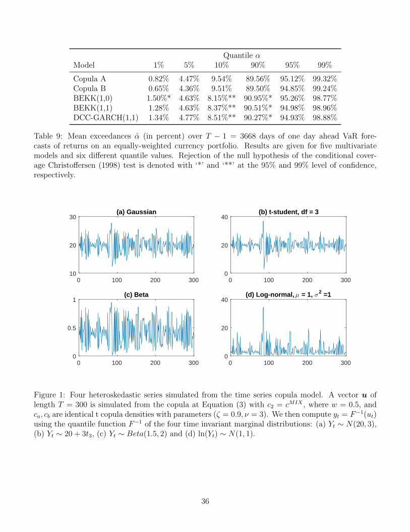
Quantile αModel 1% 5% 10% 90% 95% 99%

Copula A 0.82% 4.47% 9.54% 89.56% 95.12% 99.32%Copula B 0.65% 4.36% 9.51% 89.50% 94.85% 99.24%BEKK(1,0) 1.50%* 4.63% 8.15%** 90.95%* 95.26% 98.77%BEKK(1,1) 1.28% 4.63% 8.37%** 90.51%* 94.98% 98.96%DCC-GARCH(1,1) 1.34% 4.77% 8.51%** 90.27%* 94.93% 98.88%

Table 9: Mean exceedances α (in percent) over T − 1 = 3668 days of one day ahead VaR fore-casts of returns on an equally-weighted currency portfolio. Results are given for five multivariatemodels and six different quantile values. Rejection of the null hypothesis of the conditional cover-age Christoffersen (1998) test is denoted with ‘*’ and ‘**’ at the 95% and 99% level of confidence,respectively.

0 100 200 30010

20

30(a) Gaussian

0 100 200 3000

0.5

1(c) Beta

0 100 200 3000

20

40(b) t-student, df = 3

0 100 200 3000

20

40(d) Log-normal, μ = 1, σ2 =1

Figure 1: Four heteroskedastic series simulated from the time series copula model. A vector u oflength T = 300 is simulated from the copula at Equation (3) with c2 = cMIX , where w = 0.5, andca, cb are identical t copula densities with parameters (ζ = 0.9, ν = 3). We then compute yt = F−1(ut)using the quantile function F−1 of the four time invariant marginal distributions: (a) Yt ∼ N(20, 3),(b) Yt ∼ 20 + 3t3, (c) Yt ∼ Beta(1.5, 2) and (d) ln(Yt) ∼ N(1, 1).

36

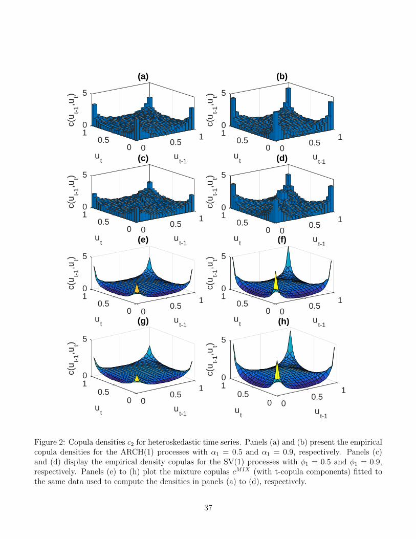
01 1

c(u

t-1,u

t)(a)

ut

0.5

ut-1

5

0.50 0

01 1

c(u

t-1,u

t)

(b)

ut

0.5

ut-1

5

0.50 0

01 1

c(u

t-1,u

t)

(c)

ut

0.5

ut-1

5

0.50 0

01 1

c(u

t-1,u

t)

(d)

ut

0.5

ut-1

5

0.50 0

01 1

c(u

t-1,u

t)

(e)

ut

0.5

ut-1

5

0.50 0

01 1

c(u

t-1,u

t)

(f)

ut

0.5

ut-1

5

0.50 0

01 1

c(u

t-1,u

t)

(g)

ut

0.5

ut-1

5

0.50 0

01 1

c(u

t-1,u

t)

(h)

ut

0.5

ut-1

5

0.50 0

Figure 2: Copula densities c2 for heteroskedastic time series. Panels (a) and (b) present the empiricalcopula densities for the ARCH(1) processes with α1 = 0.5 and α1 = 0.9, respectively. Panels (c)and (d) display the empirical density copulas for the SV(1) processes with φ1 = 0.5 and φ1 = 0.9,respectively. Panels (e) to (h) plot the mixture copulas cMIX (with t-copula components) fitted tothe same data used to compute the densities in panels (a) to (d), respectively.

37

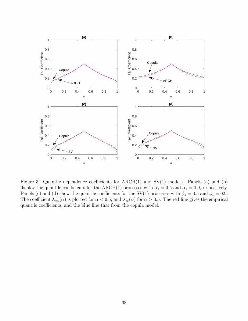
0 0.2 0.4 0.6 0.8 1α

0

0.2

0.4

0.6

0.8

1T

ail C

oeffi

cien

t(a)

0 0.2 0.4 0.6 0.8 1α

0

0.2

0.4

0.6

0.8

1

Tai

l Coe

ffici

ent

(b)

0 0.2 0.4 0.6 0.8 1α

0

0.2

0.4

0.6

0.8

1

Tai

l Coe

ffici

ent

(c)

0 0.2 0.4 0.6 0.8 1α

0

0.2

0.4

0.6

0.8

1

Tai

l Coe

ffici

ent

(d)

SVSV

CopulaCopula

Copula

Copula

ARCHARCH

Figure 3: Quantile dependence coefficients for ARCH(1) and SV(1) models. Panels (a) and (b)display the quantile coefficients for the ARCH(1) processes with α1 = 0.5 and α1 = 0.9, respectively.Panels (c) and (d) show the quantile coefficients for the SV(1) processes with φ1 = 0.5 and φ1 = 0.9.The coefficient λlow(α) is plotted for α < 0.5, and λup(α) for α > 0.5. The red line gives the empiricalquantile coefficients, and the blue line that from the copula model.

38

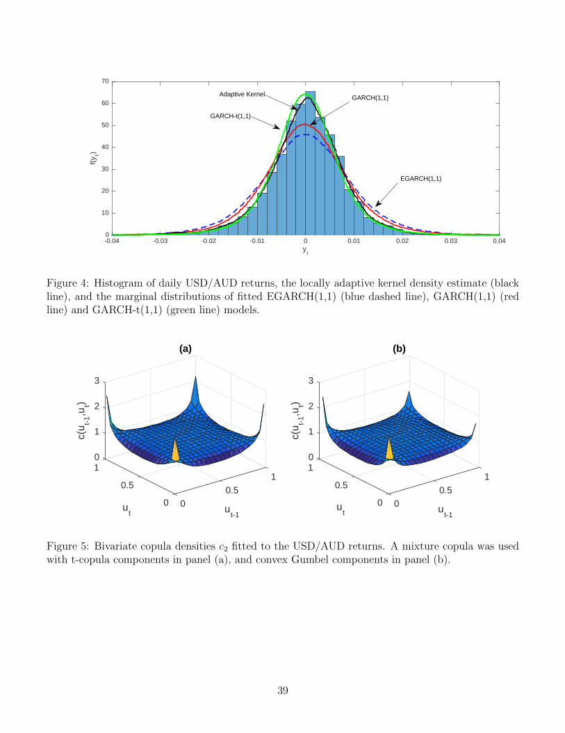
-0.04 -0.03 -0.02 -0.01 0 0.01 0.02 0.03 0.04y

t

0

10

20

30

40

50

60

70

f(y t)

Adaptive Kernel

EGARCH(1,1)

GARCH(1,1)

GARCH-t(1,1)

Figure 4: Histogram of daily USD/AUD returns, the locally adaptive kernel density estimate (blackline), and the marginal distributions of fitted EGARCH(1,1) (blue dashed line), GARCH(1,1) (redline) and GARCH-t(1,1) (green line) models.

01

1

1

c(u

t-1,u

t) 2

(a)

ut

0.5

ut-1

3

0.50 0

01

1

1

c(u

t-1,u

t) 2

(b)

ut

0.5

ut-1

3

0.50 0

Figure 5: Bivariate copula densities c2 fitted to the USD/AUD returns. A mixture copula was usedwith t-copula components in panel (a), and convex Gumbel components in panel (b).

39

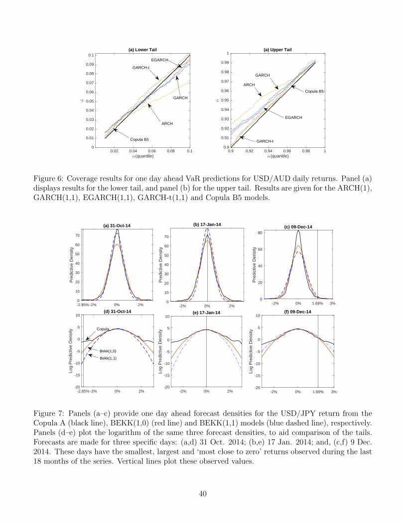
0.02 0.04 0.06 0.08 0.1α(quantile)

0

0.01

0.02

0.03

0.04

0.05

0.06

0.07

0.08

0.09

0.1

α

(a) Lower Tail

0.9 0.92 0.94 0.96 0.98 1α(quantile)

0.9

0.91

0.92

0.93

0.94

0.95

0.96

0.97

0.98

0.99

1

α

(a) Upper Tail

GARCH-t

GARCH

EGARCH

ARCH

Copula B5

GARCH

ARCH

Copula B5

GARCH-t

EGARCH

Figure 6: Coverage results for one day ahead VaR predictions for USD/AUD daily returns. Panel (a)displays results for the lower tail, and panel (b) for the upper tail. Results are given for the ARCH(1),GARCH(1,1), EGARCH(1,1), GARCH-t(1,1) and Copula B5 models.

-2.85% -2% 0% 2%-20

-15

-10

-5

0

5

10

Log

Pre

dict

ive

Den

sity

(d) 31-Oct-14

-2.85%-2% 0% 2%0

10

20

30

40

50

60

70

Pre

dict

ive

Den

sity

(a) 31-Oct-14

-2% 0% 1.69% 3%-20

-15

-10

-5

0

5

10

Log

Pre

dict

ive

Den

sity

(f) 09-Dec-14

-2% 0% 1.69% 3%0

20

40

60

80

Pre

dict

ive

Den

sity

(c) 09-Dec-14

-2% 0% 2%-20

-15

-10

-5

0

5

10

Log

Pre

dict

ive

Den

sity

(e) 17-Jan-14

-2% 0% 2%0

10

20

30

40

50

60

70

Pre

dict

ive

Den

sity

(b) 17-Jan-14

Copula

Bekk(1,1)

Bekk(1,0)

Figure 7: Panels (a–c) provide one day ahead forecast densities for the USD/JPY return from theCopula A (black line), BEKK(1,0) (red line) and BEKK(1,1) models (blue dashed line), respectively.Panels (d–e) plot the logarithm of the same three forecast densities, to aid comparison of the tails.Forecasts are made for three specific days: (a,d) 31 Oct. 2014; (b,e) 17 Jan. 2014; and, (c,f) 9 Dec.2014. These days have the smallest, largest and ‘most close to zero’ returns observed during the last18 months of the series. Vertical lines plot these observed values.

40

Online Appendix for ‘Time Series Copulas for Heteroskedas-

tic Data’

Part A of this online appendix provides a comparison of the vine copula and an ARCH(3) model,

while Part B provides some additional output from the empirical analysis in the manuscript.

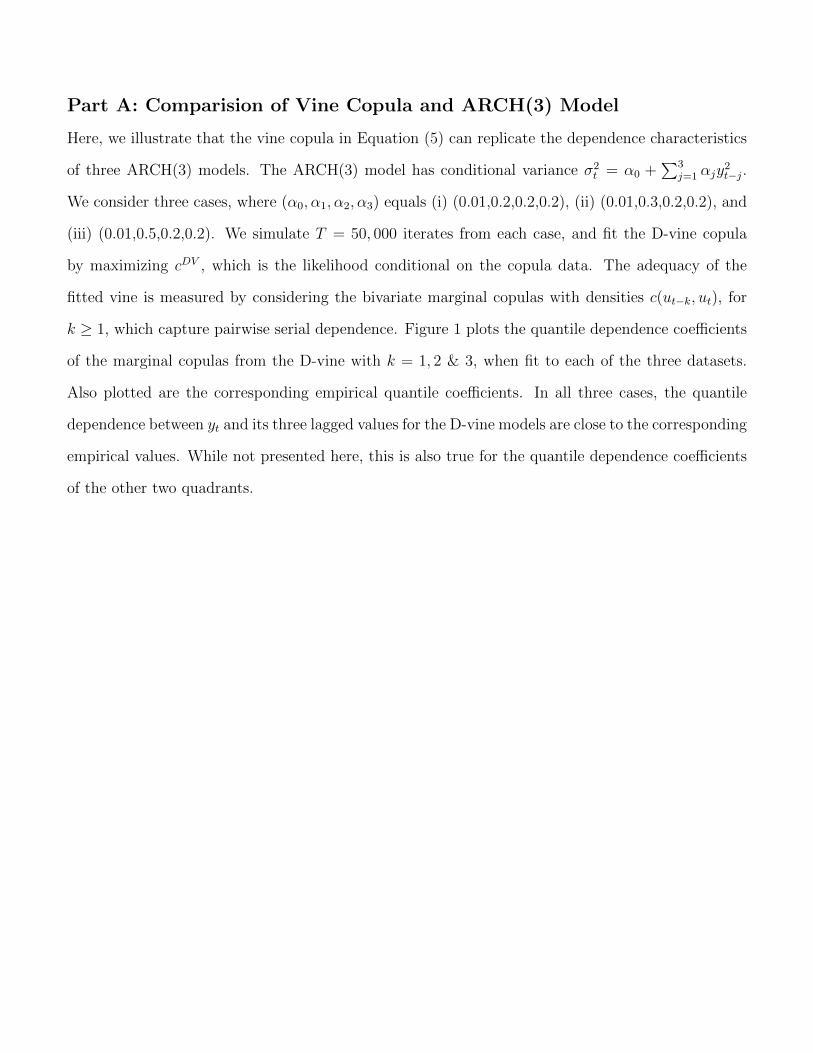
Part A: Comparision of Vine Copula and ARCH(3) Model

Here, we illustrate that the vine copula in Equation (5) can replicate the dependence characteristics

of three ARCH(3) models. The ARCH(3) model has conditional variance σ2t = α0 +

∑3j=1 αjy

2t−j.

We consider three cases, where (α0, α1, α2, α3) equals (i) (0.01,0.2,0.2,0.2), (ii) (0.01,0.3,0.2,0.2), and

(iii) (0.01,0.5,0.2,0.2). We simulate T = 50, 000 iterates from each case, and fit the D-vine copula

by maximizing cDV , which is the likelihood conditional on the copula data. The adequacy of the

fitted vine is measured by considering the bivariate marginal copulas with densities c(ut−k, ut), for

k ≥ 1, which capture pairwise serial dependence. Figure 1 plots the quantile dependence coefficients

of the marginal copulas from the D-vine with k = 1, 2 & 3, when fit to each of the three datasets.

Also plotted are the corresponding empirical quantile coefficients. In all three cases, the quantile

dependence between yt and its three lagged values for the D-vine models are close to the corresponding

empirical values. While not presented here, this is also true for the quantile dependence coefficients

of the other two quadrants.

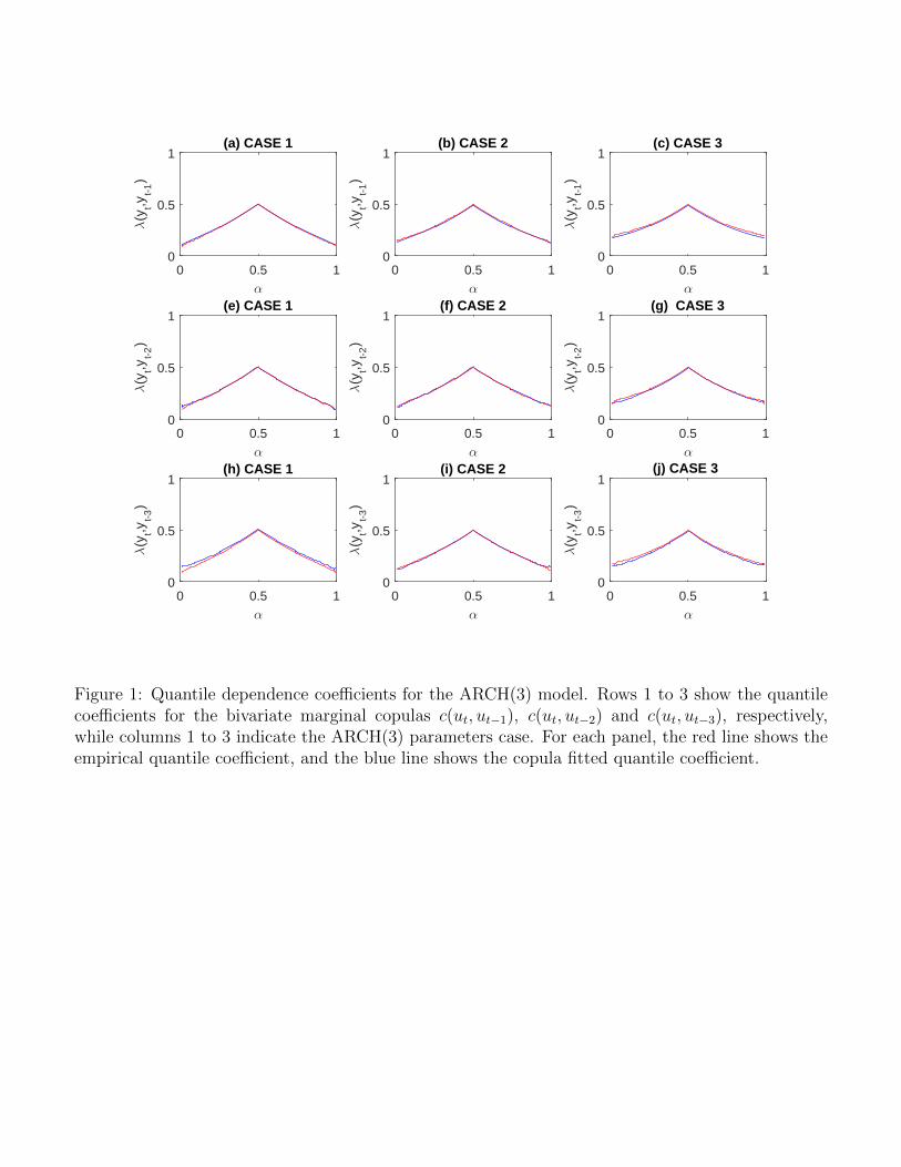
0 0.5 1α

0

0.5

1λ

(yt,y

t-1)

(a) CASE 1

0 0.5 1α

0

0.5

1

λ(y

t,yt-

2)

(e) CASE 1

0 0.5 1α

0

0.5

1

λ(y

t,yt-

3)

(h) CASE 1

0 0.5 1α

0

0.5

1

λ(y

t,yt-

1)

(b) CASE 2

0 0.5 1α

0

0.5

1

λ(y

t,yt-

2)

(f) CASE 2

0 0.5 1α

0

0.5

1

λ(y

t,yt-

3)

(i) CASE 2

0 0.5 1α

0

0.5

1

λ(y

t,yt-

1)

(c) CASE 3

0 0.5 1α

0

0.5

1

λ(y

t,yt-

2)

(g) CASE 3

0 0.5 1α

0

0.5

1

λ(y

t,yt-

3)

(j) CASE 3

Figure 1: Quantile dependence coefficients for the ARCH(3) model. Rows 1 to 3 show the quantilecoefficients for the bivariate marginal copulas c(ut, ut−1), c(ut, ut−2) and c(ut, ut−3), respectively,while columns 1 to 3 indicate the ARCH(3) parameters case. For each panel, the red line shows theempirical quantile coefficient, and the blue line shows the copula fitted quantile coefficient.

Part B: Additional Empirical Output

Model ζa > 0 νa ζb > 0 νb w

ARCH (α0 = 0.01, α1 = 0.5) 0.705 39.996 0.179 2.984 0.191(α0 = 0.01, α1 = 0.9) 0.678 6.004 0.701 7.044 0.509

SV (φ1 = 0.5, σ2 = 2.5, h = 0.8) 0.454 20.019 0.555 39.994 0.547(φ1 = 0.9, σ2 = 2, h = 0.8) 0.693 10.740 0.728 15.031 0.512

Table 1: MLE parameter estimates for mixture of t copulas fitted to ARCH(1) and SV(1) models.

0 0.2 0.4 0.6 0.8 1

α

0

0.2

0.4

0.6

0.8

1

Tai

l Coe

ffici

ent

(a)

0 0.2 0.4 0.6 0.8 1

α

0

0.2

0.4

0.6

0.8

1

Tai

l Coe

ffici

ent

(b)

0 0.2 0.4 0.6 0.8 1

α

0

0.2

0.4

0.6

0.8

1

Tai

l Coe

ffici

ent

(c)

0 0.2 0.4 0.6 0.8 1

α

0

0.2

0.4

0.6

0.8

1

Tai

l Coe

ffici

ent

(d)

Copula

Copula

Copula

Copula

ARCH ARCH

ARCH

ARCH

Figure 2: The off-diagonal quantile dependence coefficients λLU(α) ≡ Pr(ut > (1− α)|ut−1 < α) andλUL(α) ≡ Pr(ut < (1 − α)|ut−1 > α) for the ARCH(1) and SV(1) models in Section 2.1. Panels(a) and (b) display the quantile coefficients for the ARCH(1) processes with α1 = 0.5 and α1 = 0.9,respectively. Panels (c) and (d) show the quantile coefficients for the SV(1) processes with φ1 = 0.5and φ1 = 0.9. The coefficient λLU(α) is plotted to left of α = 0.5, and λUL(α) to the right. The redline gives the empirical quantile coefficients, and the blue line that from the copula model.

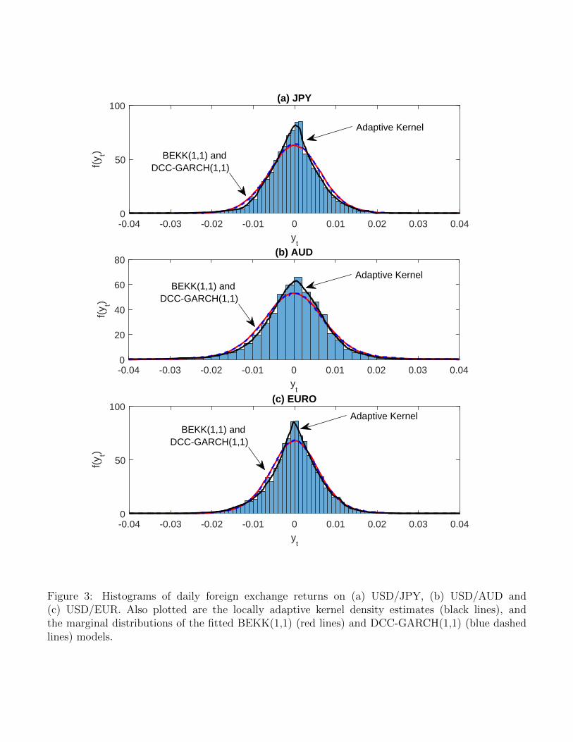
-0.04 -0.03 -0.02 -0.01 0 0.01 0.02 0.03 0.04y

t

0

50

100f(

y t)(a) JPY

-0.04 -0.03 -0.02 -0.01 0 0.01 0.02 0.03 0.04y

t

0

20

40

60

80

f(y t)

(b) AUD

-0.04 -0.03 -0.02 -0.01 0 0.01 0.02 0.03 0.04y

t

0

50

100

f(y t)

(c) EURO

Adaptive Kernel

Adaptive Kernel

Adaptive Kernel

BEKK(1,1) and DCC-GARCH(1,1)

BEKK(1,1) and DCC-GARCH(1,1)

BEKK(1,1) and DCC-GARCH(1,1)

Figure 3: Histograms of daily foreign exchange returns on (a) USD/JPY, (b) USD/AUD and(c) USD/EUR. Also plotted are the locally adaptive kernel density estimates (black lines), andthe marginal distributions of the fitted BEKK(1,1) (red lines) and DCC-GARCH(1,1) (blue dashedlines) models.

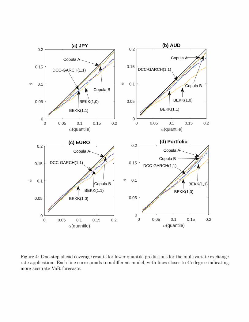
0 0.05 0.1 0.15 0.2

α(quantile)

0

0.05

0.1

0.15

0.2

α

(a) JPY

0 0.05 0.1 0.15 0.2

α(quantile)

0

0.05

0.1

0.15

0.2

α

(b) AUD

0 0.05 0.1 0.15 0.2

α(quantile)

0

0.05

0.1

0.15

0.2

α

(c) EURO

0 0.05 0.1 0.15 0.2

α(quantile)

0

0.05

0.1

0.15

0.2

α

(d) Portfolio

BEKK(1,1)

Copula A

DCC-GARCH(1,1)

BEKK(1,0)

Copula B

Copula A

Copula A Copula A

Copula B

Copula B

BEKK(1,0)

BEKK(1,0)

BEKK(1,0)

BEKK(1,1)

BEKK(1,1)

Copula B

BEKK(1,1)

DCC-GARCH(1,1)

DCC-GARCH(1,1)DCC-GARCH(1,1)

Figure 4: One-step ahead coverage results for lower quantile predictions for the multivariate exchangerate application. Each line corresponds to a different model, with lines closer to 45 degree indicatingmore accurate VaR forecasts.

0.8 0.85 0.9 0.95 1

α(quantile)

0.8

0.85

0.9

0.95

1

α

(a) JPY

0.8 0.85 0.9 0.95 1

α(quantile)

0.8

0.85

0.9

0.95

1

α

(b) AUD

0.8 0.85 0.9 0.95 1

α(quantile)

0.8

0.85

0.9

0.95

1

α

(c) EURO

0.8 0.85 0.9 0.95 1

α(quantile)

0.8

0.85

0.9

0.95

1

α

Portfolio

BEKK(1,1)

Copula A

BEKK(1,0)

DCC-GARCH(1,1)

Copula B

BEKK(1,0)

BEKK(1,1)

Copula A

DCC-GARCH(1,1)

Copula B

DCC-GARCH(1,1)

BEKK(1,1)

BEKK(1,0)

Copula B

Copula A

BEKK(1,0)

BEKK(1,1)

Copula B

Copula A

DCC-GARCH(1,1)

Figure 5: One-step ahead coverage results for upper quantile predictions for the multivariate exchangerate application. Each line corresponds to a different model, with lines closer to 45 degree indicatingmore accurate VaR forecasts.