time series data analyses in space physics table - ucla
TRANSCRIPT

TIME SERIES DATA ANALYSES IN SPACE PHYSICS
P. SONG1,2 and C. T. RUSSELL21 Space Physics Research Laboratory, The University of Michigan, Ann Arbor, MI 48109, U.S.A.;
E-mail: [email protected] Institute of Geophysics and Planetary Physics, University of California, Los Angeles, CA 90095,
U.S.A.;E-mail: [email protected]
(Received 24 July, 1997; accepted 6 February, 1998)
Abstract. Techniques of time series data analyses developed over the past decades are reviewed. Wediscuss the theoretical principles and mathematical descriptions of these analytical techniques thathave been developed by scientists with different backgrounds and perspectives. These principles notonly provide the guidelines to evaluate each particular technique but also point to directions for thedevelopment of new methods. Most time series analyses can be divided into three categories: discon-tinuity analysis, wave analysis and correlation analysis. Techniques for analyzing one-dimensionaldiscontinuities have been well-developed and tested. The errors and ambiguities of discontinuityanalyses are reasonably well, but not as widely, understood. Techniques for wave analyses have beendeveloped for certain wave properties and are still under further active development. Problems inusing these techniques are recognized to a certain extent. Because of the complicity of the waves inspace and the limitation of probing, there are significant needs for the development of new methods.Although simple techniques for two-satellite correlation analyses have been developed and tested forsome time, techniques for multiple satellites are in an embryonic stage. We expect to see significantadvances in the development of new techniques and new concepts. We believe, however, that theproblems in this area have not been fully appreciated.
Table of Contents
1. Introduction1.1. Frame of Reference1.2. Coordinate Systems1.3. Measurements and Their Uncertainties1.4. Principal Axis Analysis
2. Discontinuity Analyses2.1. Background2.2. Minimum Variance Analysis2.3. Tangential Discontinuity Analysis2.4. Coplanarity Analysis2.5. Maximum Variance Analysis2.6. DeHoffmann–Teller Frame and Walen Relation Test2.7. Suggested Procedures for Discontinuity Analysis2.8. Rankine–Hugoniot Relations Test
3. Wave Analyses3.1. Background
Space Science Reviews87: 387–463, 1999.© 1999Kluwer Academic Publishers. Printed in the Netherlands.
388 P. SONG AND C. T. RUSSELL
3.2. Routine Wave Analysis3.3. Mode Identification3.4. Frequency and Phase Velocity3.5. Nonlinear Effects3.6. Plasma Wave Analysis
4. Spatial Correlation Analyses4.1. Background4.2. One-Dimensional Discontinuity Analyses4.3. Two-Dimensional Structures4.4. Determination of Electric Currents4.5. Wave Analyses
5. Discussion and Summary
1. Introduction
Many of the observational data in space physics are obtained as time series. Thesetime series contain measured physical quantities, that may be scalars, vectors, ten-sors, or multidimensional images. Examples of such quantities are temperaturesand densities of the plasma, magnetic or electric field vectors, pressure tensors,and auroral images. These quantities can be measured either in space on a movingplatform or on a fixed platform such as the surface of the Earth. Thus the variationsin the time series may represent true temporal changes in the system or motionthrough spatial gradients or some combination of the two. Since most data gatheredin space physics are initially in the form of time series, their use is widespread. Toanalyze these time series data, many data processing methods, analysis techniquesand computer algorithms have been developed. In this review, we outline a setof principles for data analysis methods, describe a number of well-established dataanalysis techniques, discuss the uncertainties and limitations of each technique, andsuggest procedures and criteria which may reduce the uncertainties of the resultsfor some analyses. Many of the principles presented are derived for the first time.
Most time-series analyses can be divided into three categories: discontinuityanalysis, wave analysis, and correlation analysis. Discontinuity analysis determinesthe orientation, thickness and motion of the interface between two different plasmaregions or regimes. The methods for discontinuity analysis are well developed.However, due to the lack of wide recognition of the underlying assumptions, un-certainties and validity of each method, there are still many problems in this area.We present a comprehensive discussion of these problems. Wave analysis deter-mines the properties and characteristics of a wave that identify which of the severalpossible wave modes allowed in a plasma a particular observed fluctuation mightbe. Techniques for wave analysis are under active development. We discuss theprinciples of these methods. Since discontinuities can be considered as steepenedwaves, some of the methods for wave analysis can be used in discontinuity analysis.Correlation analysis determines the relationship between observations at two ormore spatially separated locations. Correlation studies can be performed in the

TIME SERIES DATA ANALYSES IN SPACE PHYSICS 389
time domain, for example to determine the time lags between observers. Correla-tion analysis can also be performed in the frequency domain. We will give a briefintroduction to correlation analysis and discuss how to apply it to the analysis ofthe data from a cluster of satellites.
From the beginning of the space age, scientists have sought means for quickqualitative visual examination of large amounts of data. With plotted traces, onecan easily spot a discontinuity, estimate a wave frequency and correlate two tracesby overlaying them. Even today these qualitative visual analyses can be powerfulways to check the results of an analysis, i.e., a quantitative result is suspicious ifone cannot verify the consistency of the result by visual inspection of the data. Aswill be stressed in this paper, relying solely on automated computer analysis maylead to completely wrong results. As a data analyst, one has to frequently return tothe examination of the original observations to perform what is often referred to asa ‘sanity check’ or a ‘reality check’.
The first quantitative data analysis method for discontinuities was the mini-mum variance analysis for discontinuity analysis proposed by Sonnerup and Cahill(1967). In the 1970s, the wave analysis techniques using the magnetic field becamemature. Along with the improvements of the plasma measurements, in the 1980sand 1990s, techniques incorporating plasma measurements have been under activedevelopment. The correlation analysis of signals made at two or more observationsites has become important since the launches of the ISEE satellites and it willplay the key role in analyzing the multiple satellites data in the International SolarTerrestrial Physics (ISTP) program. While in theory the quantitative correlationanalysis is most straightforward compared with other analyses, in practice, thereare many problems associated with the coherence length of a phenomenon, com-pared with the spacecraft separation, for example. We suspect that many problemshave not yet even been recognized. In the next few years, we expect to see majorprogress in understanding of correlation analyses as a result of multiple-satellitedata analyses.
1.1. FRAME OF REFERENCE
Observational data are gathered in a frame of reference at rest with the observer.Physical laws are often stated in a frame of reference that is moving with respect tothe observer. In particular, the Rankine–Hugoniot relations are given in the frame ofreference at rest with the discontinuity, and the wave dispersion relations usuallyexpressed in the plasma rest frame. In the non-relativistic limit, plasma density,pressure, magnetic field, and wavelength are not dependent on the frame of refer-ence, but velocity, electric field, and frequency are. While it is always important towork in the appropriate frame of reference when dealing with a flowing plasma,this is critically true in the supersonic solar wind.
The total time derivative of an observed quantityQ, which can be either a scalaror a vector, is
390 P. SONG AND C. T. RUSSELL
DQ
Dt= ∂Q
∂t+ (v · ∇)Q , (1.1)
wherev is the velocity of the observer relative to the frame of reference in whichthe phenomena is described. The first term on the right is the temporal variationin the frame of reference of the plasma (say) and the second term on the right isthe apparent temporal variation caused by motion through spatial gradients. Bothare observed by a moving instrument as temporal variations. For example, whendiscussing observations of a wave in the plasma frame,v is the measured plasmaflow velocity, and the∂/∂t term is nonzero. For a steady phenomenon, the∂/∂t
term is zero (e.g., in the plasma frame) and the observed time variation is due to themotion through stationary gradients. A time-domain correlation analysis assumesthat, in a particular frame, for example, a wave frame or a shock frame,∂/∂t =0. Therefore the velocity derived from the timing difference is the sum of the flow(convection) velocity and the propagation (phase) velocity. We recall that the groupvelocity measures the velocity of the envelope of the variations whereas the varia-tions themselves move at the phase velocity. The energy of the wave packet flowswith the group velocity and it is the group velocity that is restricted to velocitiesequal to or less than the speed of light, not the phase velocity.
For magnetic field measurements, using the frozen-in Faraday’s law and diver-gence free condition, Equation (1.1) becomes,
DBDt= (B · ∇)v− (∇ · v)B . (1.2)
Assume a coordinate system,m, n with variations only along the normal or a di-rection under one-dimensional assumption, for either a discontinuinty or a wave, inwhich ∂/∂` and∂/∂m are zero. It is easy to show that the measured time variationof the field is zero in the direction alongn. No stationarity assumption is made hereand this is true independent of the frame of reference. This particular feature of themagnetic field is actually the basis of most data analysis techniques. Note that indiscontinuity analysis, one cannot always assume that the shock frame is known,nor in wave analysis, that the wave is in steady state.
For other quantities, temporal variations in the frame in which a theory is ap-plied, may affect the results of an analysis. For example, the observed electric fieldvariation is
DEDt= ∂E′
∂t+∇(v · E′)− ∂v
∂t× B , (1.3)
whereE′ = E + v × B is the electric field in the frame of reference in whichthe phenomenon is described. Note here that∇ × E = −∂B/∂t and we haveassumedv to be uniform in space. Whenv is not spatially uniform, more termsappear. Under a 1-D assumption, neither component is zero in general. But for1-D steady state, the tangential components of the variation vanish whereas thenormal component does not. This property of the electric field variation provides

TIME SERIES DATA ANALYSES IN SPACE PHYSICS 391
the foundation of the maximum variance analysis to be discussed in Section 2.5.Note that this method requires the steady state assumption and thus is difficult toapply to wave analyses. For discontinuity analysis, not only unsteadiness of thediscontinuity but also changes in the motion of the discontinuity relative to theobserver affect the results. Since in space, boundaries are often in oscillation andnot in simple motion, only on a few occasions is the latter effect unimportant. Whencomparing measurements from two spacecraft at different times, more effects willoccur due to the relative motion between the spacecraft frame and the plasma frame(see more discussion in Section 4.1.3).
1.2. COORDINATE SYSTEMS
1.2.1. Global Coordinate SystemsThree global coordinate systems are often used in space physics. A global coordi-nate system is useful for studying phenomena of global effects.
1.2.1.1. GSE coordinate system.In the Geocentric-Solar-Ecliptic coordinate sys-tem, thex direction is from the Earth to the Sun. Thez direction is along the normalto the ecliptic plane and pointing to the north. They direction completes the righthanded coordinate system and points to the east, opposite planetary motion. Thestatistical aberration of the solar wind by the Earth’s orbital motion is most readilyremoved in this system. It is useful for problems in which the orientation of theEarth’s dipole axis is not important, such as the bow shock and magnetosheathphenomena.
1.2.1.2. GSM coordinate system.In the Geocentric-Solar-Magnetospheric coor-dinate system, thex direction is also from the Earth to the Sun. Thez directionlies in the plane containing the Sun–Earth line and the geomagnetic dipole, andis perpendicular to the Sun–Earth line and positive north of the Sun–Earth line.They direction completes the right-handed coordinate system. The GSMy andzdirections lie at an acute angle (around thex direction) to the GSE counterparts.The GSM coordinates are most useful for studies of solar wind-magnetosphere in-teraction and where the solar wind determines the geometry of the magnetosphere.These include phenomena near and at the magnetopause/boundary layer, in theouter magnetosphere and near earth magnetotail.
1.2.1.3. SM coordinate system.In the Solar Magnetic coordinate system, thezdirection is along the Earth’s magnetic dipole pointing north. Thex − z planecontains the solar direction with roughly toward the Sun. Itsy direction is onthe dawn-dusk meridian and points to dusk in the same direction as the GSMy
direction. Thus the SMx andz directions differ from their GSM counterparts byan acute angle of rotation related to the tilt of the dipole. The SM coordinates areusually used in studies of the near earth phenomena, where the geomagnetic field

392 P. SONG AND C. T. RUSSELL
Figure 1.1.Boundary normal coordinate system (Russell and Elphic, 1978).
controls the processes, such as the ionosphere, inner magnetosphere, and groundobservations.
1.2.2. Local Coordinate SystemsTo study a local phenomenon or a global phenomenon in a local context, a localcoordinate system is most convenient. Three local coordinate systems are oftenused in the literature.
1.2.2.1. Boundary normal coordinate system (LMN) (Russell and Elphic, 1978).TheN direction is along the normal of the boundary, which can be the bow shock orthe magnetopause, or a current sheet. The direction is usually chosen to be outwardfrom the Earth for both the bow shock and the magnetopause. TheL directionis along the geomagnetic field direction for the magnetopause and is along theprojection of the upstream magnetic field on the boundary for the bow shock. TheM direction completes the right-handed coordinate system and points to dawn forthe magnetopause (see Figure 1.1). At the subsolar magnetopause, neglecting theaberration caused by the finite velocity (29.5 km s−1) of the Earth through thesolar wind, the LMN coordinates are coincident with the GSM coordinates withN → x, L→ z andM →−y.
The LMN coordinate system is useful only locally unless the boundary is planar.In some cases, a satellite may move along a curved boundary, e.g., the magne-topause, for a long period of time and cross it many times as the boundary rocksback and forth. The normal of the boundary at each crossing may be different.

TIME SERIES DATA ANALYSES IN SPACE PHYSICS 393
When presenting the data in a fixed LMN coordinate system, one needs to beextremely careful in interpreting the results because the direction of the normalof the boundary may be varying. Similarly one should be cautious in using anLMN coordinate system derived from either the magnetopause or bow shock wellaway from that boundary such as in presenting the data from the bow shock to themagnetopause. One should not interpret, for example, theN component along adirection determined at the magnetopause as the normal component throughout themagnetosheath.
1.2.2.2. Field-aligned coordinate system.The average magnetic field direction(taken from thein situ measurements) is defined as a preferential direction. Asecond direction is usually defined according to the symmetry of the system. Forexample, for magnetospheric wave studies, the azimuthal direction parallel to thedirection obtained from the cross product of the magnetic field and the radiallyoutward direction is usually used as the second direction. This direction is eastwardin the Earth’s magnetosphere in the direction of electron drift. This direction isuseful for displaying the field perturbations associated with sheets of field alignedcurrents that are roughly along shells of constant L-value or L-shells. Similarly,for magnetosheath studies, one can define a surface in the sheath which belongsto the family curves that are used for empirical models of the magnetopause andbow shock. The second direction can then be defined perpendicular to the field andalong the surface.
1.2.2.3. Geomagnetic dipole coordinate system.The Geomagnetic Dipole coor-dinate system has itsz direction along the geomagnetic dipole axis. The other twodirections are defined in terms of geomagnetic latitude and longitude by analogywith geographic coordinates. Therefore, this coordinate system is useful in study-ing phenomena observed in ionosphere and ground stations. In order to study theglobal effects of these phenomena, an observation is often presented in geomag-netic local time, which is equivalent to that in SM coordinates, and is the anglebetween the meridian plane containing the Sun and that containing the point ofobservation converted to hours and increased by 12 hours.
1.2.3. Spacecraft Coordinate SystemFor some vector quantities only two components are measured by our spacecraft.Examples are the electric field, plasma waves and the plasma moments from certaininstruments. The two components are in the plane perpendicular to the space-craft spin axis. Frequently, the spin axis is nearly along one of the GSE axes (formagnetospheric missions) or perpendicular to the orbit plane (cartwheel mode forionospheric missions). The fraction and the direction of the background magneticfield projected onto this plane are important to observations which deal with theanisotropies with respect to the magnetic field. The spin modulation of the high

394 P. SONG AND C. T. RUSSELL
time resolution signals can provide useful information. Often artifacts in measure-ments are most easily detected in spacecraft coordinates.
1.3. MEASUREMENTS AND THEIR UNCERTAINTIES
A measured physical quantity is derived from measureable quantities by a instru-ment. Therefore, its accuracy is limited by the instrument capability and the datareduction procedures. As a data analyst, it is very important to understand theprinciples of the instruments from which the data are measured and the schemesof the data reduction that are used. In this section, we will discuss several generalissues concerning the measurements and data reduction. We will assume that themeasurements are accurate in other sections in the paper. The word ‘fluctuation’used in this paper refers to deviations from the average of the measured quantity.The word ‘noise’ refers to the unwanted signals that are not described by the ideal-ized variations of a particular analysis method. It is important to point out that the‘noise’ in one analysis can be a physical phenomenon for another analysis. Fluctu-ations include both wanted signals and noise. If one chooses a wrong method, theuseful signals will be treated as noise.
1.3.1. Resolutions1.3.1.1. Time resolution. Temporal resolution, the time between samples, is amajor limit in many data analysis methods. For example, to use the MinimumVariance method (to be discussed in Section 2.2) requires the resolution to be atleast half of the crossing duration of a discontinuity, i.e., one needs a sample inthe middle of the crossing not just at either end. Temporal resolution also setsan upper cutoff frequency, the so-called Nyquist frequency, which is half of thesampling frequency, for Fourier analysis. Stated differently, in order to resolve awaveform, the sampling frequency should be at least twice the wave frequency. Iffrequencies above the Nyquist frequency are present when a signal is digitized itappears to oscillate at the frequency below the Nyquist requency. Such a signal iscalled aliased. The timing difference derived from correlation analysis is limitedby the accuracy of the clocks controling the measurements. Synchronization ofclocks of observers becomes very important when the timing differences are small.Sometimes components of vectors are not sampled simultaneously. Sometimes thetime separation of sequential measurements is not uniform. Techniques exist foraccurately analyzing signals under these circumstances but add complexity to theanalysis.
If the bandwidth of the measurements is large compared to the frequency rangeof the phenomenon of interest, i.e., if the temporal resolution is too high, timedomain analysis (which accept signals of any frequency) will be affected by ‘un-wanted signals.’ For example, if within a discontinuity, there are waves which arepolarized in the normal direction of the discontinuity, they will affect the resultof a Minimum Variance analysis. Although these high frequency phenomena have
TIME SERIES DATA ANALYSES IN SPACE PHYSICS 395
their own physical significance they may be treated as ‘noise’ in analysis of low-frequency phenomena. Therefore, in time domain analysis proper preparation ofthe data by either running average or filtering is important to limit the band ofinformation to the time scale of the phenomenon of interest.
1.3.1.2. Amplitude resolution. Digitized measurements have finite amplitude res-olution as well as finite temporal resolution. The result of the process is to add asquare wave, or finite steps to the data. When a Fourier analysis is performed bydigitized data, there is a minimum noise level set by the digitization ofD2/12FN ,whereFN is the Nyquist frequency andD is the digital window. This digital noise isspread uniformly over the bandwidth of the signal, i.e., 0 toFN and when decreas-ing the bandwidth of the digitized signal by subsampling or ‘decimating’ as it issometime called, it is important to low-pass filter the signal, or else the entire digitalnoise of the original time series will be added to the new narrower bandwidth. Ifthe digital noise is comparable to the measured signal, the noise is most readilyreduced by digitizing more finely than increasing bandwidth (Russell, 1972).
1.3.2. Field MeasurementsOne of the most accurately determined quantities in space is the magnetic field, ifattention is paid to considerations of linearity, magnetic cleanliness and bandwidthrelative to the Nyquist frequency. For an elliptical Earth orbiter its magnitude canbe calibrated each time at perigee where the field is known and the zero levelsof each sensor in the spin plane can be calibrated as the spacecraft rotates (e.g.,Kepko et al., 1996). The intercalibration among different spacecraft can be done incurrent-free regions (e.g., Khurana et al., 1996).
The electric field measurements are affected by spacecraft charge and Debyelength. The understanding of the calibration problem has been significantly im-proved and the validity of the measurements has been tested (Mozer et al., 1979,1983). Nevertheless, special caution should be taken in the regions with significantplasma gradients and low plasma density.
High frequency (>10 Hz) electric field fluctuations are measured with electricdipole antennae. Often only the components in the spin plane are measured. Thereliability of the data is generally good. The major limitation is caused by thefinite data rate which results in competition between the frequency and temporalresolutions. For example, to infer the plasma density from waves at the plasmafrequency, one needs a fine frequency resolution, but to determine the polariza-tion of a wave based on spin modulation, one needs a temporal resolution a fewtimes the spacecraft spin period. The corresponding oscillating magnetic field isusually measured with wire coil antennae that are sensitive to the time derivativeof the magnetic field. A search coil magnetometer is a coil antenna with a highlypermeable core and is used at ELF and VLF frequencies, say 10 to 104 Hz.

396 P. SONG AND C. T. RUSSELL
1.3.3. Plasma MomentsA plasma detector measures the number of particles1N in an energy range be-tweenU andU +1U that tranverse in a time1t an area1A within an element ofsolid angle1� around the normal toA. The differential direction (flux) intensityis defined as
J = 1N/(1A1�1U1t) (1.4)
In principle,1A is the cross-section of the detector,1� and1U are the angularand energy resolutions of the instrument, and1t is the sampling time which equalsthe data rate for continuous measurements. To obtain a complete distribution func-tion, the instrument has to scan all look-directions and energy ranges. Often theangular and energy resolutions (and the signal-noise ratio) compete for the limitedtelemetry.
The plasma distribution functionf is related toJ by (1N = f1v1r , U =12mv
2,1r = v1A1t,1v = v21�1v),
f = m
v2J , (1.5)
wherem andv are the mass and velocity of a particle being detected. With thedistribution function, the plasma moments, density, velocity, pressure and heat flux(for a particular species), can be derived,
N =vHC∑vLC
∑�
f v21�1v , (1.6)
V = 1
N
vHC∑vLC
∑�
vf v21�1v , (1.7)
P = mvHC∑vLC
∑�
(v− V)2f v21�1v , (1.8)
T = P/N , (1.9)
wherevLC andvHC are the lower and higher cutoff velocities that are determinedby the lower and higher cutoff energies,ELC andEHC, and the spacecraft potential8, and are
vLC,HC = 2
m
√ELC,HC+ q8 , (1.10)
whereq is the electric charge of the particle. For a 2-D detector, an assumption isneeded in order to extrapolate the values of fluxes in undetected directions. Thisassumption becomes important when the anisotropy of the plasma is high. Note

TIME SERIES DATA ANALYSES IN SPACE PHYSICS 397
Figure 1.2.Ratios of the measured to real moments (Song et al., 1997). The lower cutoff velocityshould be evaluated from the lower cutoff energy of the detector and the spacecraft potential at thetime. The temperatures, in eV, for1
2v2L = 20 eV ion detector and12v
2L = 15 eV electron detector,
when the spacecraft is uncharged, are given for corresponding values in thex axis. Different linesare for different bulk velocitiesv0 normalized by(2T0)
1/2, which are close to the Mach numbers.
that the effects of the spacecraft charge depend on the species and that the cutoffvelocities are very large for electrons compared with ions because of their smallmass.
The effects of a finite sampling energy range on the moment measurementsdepend on the temperature and velocity of the plasma being detected (Song et al.,1997). If the temperature is many times lower than the higher cutoff energy, thehigher cutoff has only minor effects. The lower cutoff has more extended effects.In general, see Figure 1.2, the density and pressure are underestimated, and thevelocity and temperature overestimated. In order to reduce the errors, some dataanalysts interpolate the points below the lower cutoff or fill the hole with best-fit toa convective Maxwellian distribution. The energy resolution becomes an importantissue in order to accurately derive the moments of cold plasmas. Without a good

398 P. SONG AND C. T. RUSSELL
energy resolution within the bulk of the distribution, the density cannot be derivedaccurately.
In summary, it is very important for a data analyst to understand the scheme ofthe algorithm with which plasma moments are derived. Caution should be takenin particular for electrons, cold plasmas, plasmas with large anisotropy using 2-Dmeasurements, and plasmas of multiple populations.
1.3.4. IntercalibrationFor quantitative data analyses, the calibration of a measurement becomes essential.A calibration factor is often a function of time and plasma conditions. For example,degradation of an instrument with time requires the measurements be calibratedand recalibrated, and the calibration factor may change significantly across a shockas the plasma condition differs (Sckopke et al., 1990; Song et al., 1997).
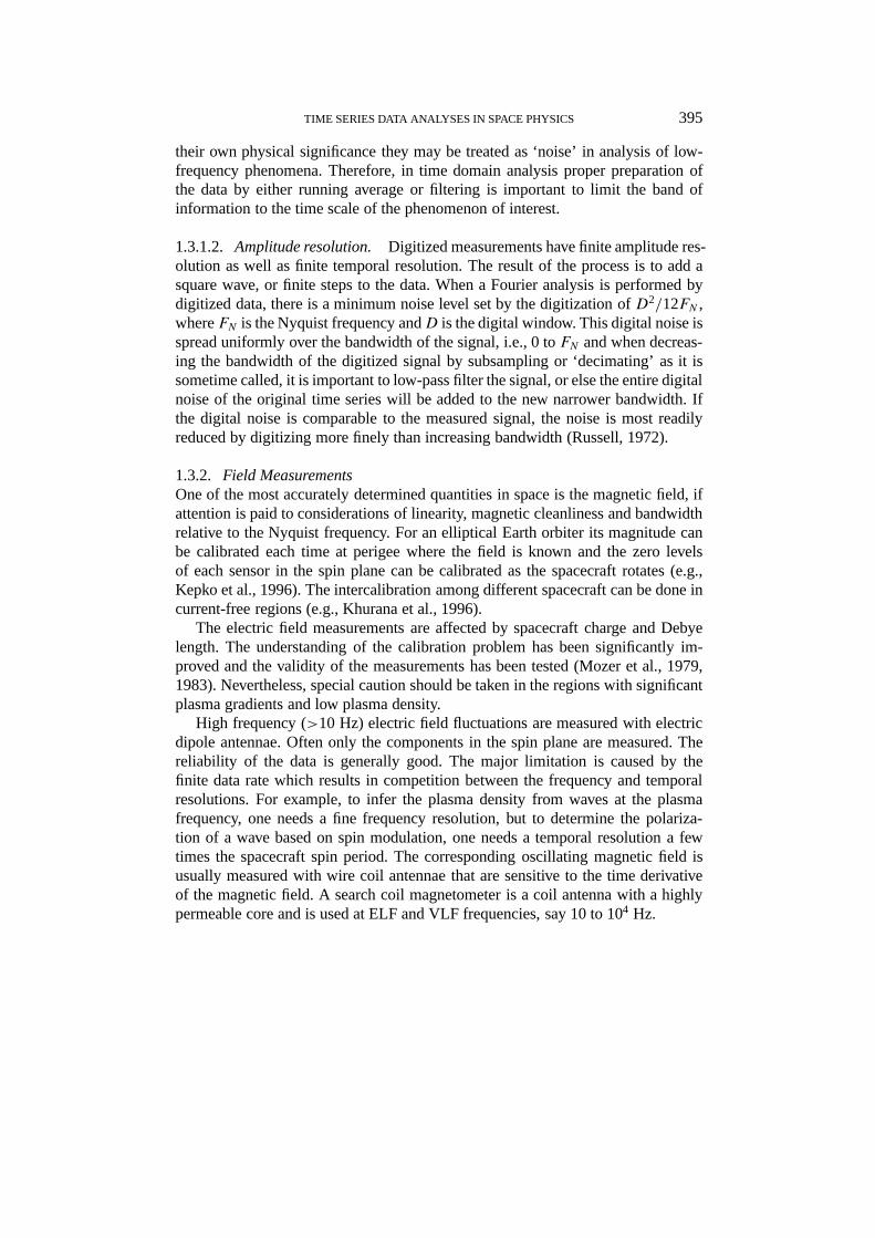
When data analysis involves more than one instrument, intercalibration amongthese instruments becomes important. For example, the sonic Mach number is theratio of two moments measured by the same detector. Even though the absolutevalue of each moment may not be accurate, one may suspect their ratio to bereasonably accurate. The Alfven Mach number, on the other hand, involves threemeasured quantities from two different instruments. The chance for error is muchgreater. Another interesting example is that the nonlinear response of two instru-ment could lead to significant differences in the same physical quantity (Petrinecand Russell, 1993) and these differences may vary with the measured parameters.One way to intercalibrate the magnetic field and plasma moments measurements isto use the force balance requirement under some known conditions, such as near astagnation region (Song et al., 1993), see Figure 1.3 and its caption.
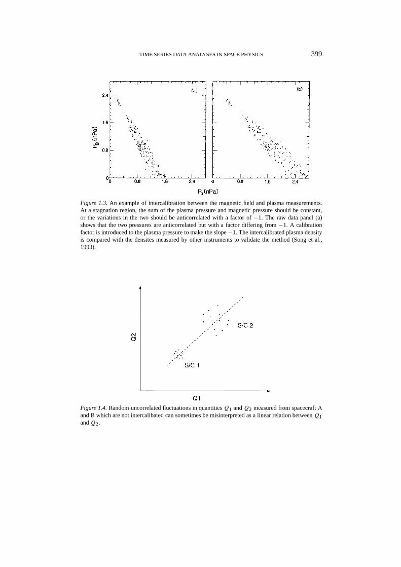
Quantitative comparison among measurements from different satellites requiresknowledge about the above issues for all satellites involved. Without careful inter-calibration, one could draw a wrong conclusion. For example, the difference incalibration for two satellites could make normal fluctuations of two physical quan-tities into two clusters which lead to a linear relationship. This relationship couldbe mistakenly interpreted as a dependence between the two physical quantities, seeFigure 1.4 for example.
Advances in technology and accumulation of experience have made multiple-instrument multiple-satellite studies possible. Plasma density can be intercalibratedby comparing particle measurements with plasma frequency measured by plasmawave experiments or wave propagation experiment (e.g. Harvey et al., 1978). Plasmavelocity can be intercalibrated by comparing particle measurements with the fieldconvection velocity,E × B (e.g., Mozer et al., 1983). However, the latter velocityhas components only perpendicular to the magnetic field.
TIME SERIES DATA ANALYSES IN SPACE PHYSICS 399
Figure 1.3.An example of intercalibration between the magnetic field and plasma measurements.At a stagnation region, the sum of the plasma pressure and magnetic pressure should be constant,or the variations in the two should be anticorrelated with a factor of−1. The raw data panel (a)shows that the two pressures are anticorrelated but with a factor differing from−1. A calibrationfactor is introduced to the plasma pressure to make the slope−1. The intercalibrated plasma densityis compared with the densites measured by other instruments to validate the method (Song et al.,1993).
Figure 1.4.Random uncorrelated fluctuations in quantitiesQ1 andQ2 measured from spacecraft Aand B which are not intercalibated can sometimes be misinterpreted as a linear relation betweenQ1andQ2.

400 P. SONG AND C. T. RUSSELL
1.4. PRINCIPAL AXIS ANALYSIS
Principal Axis Analysis provides the mathematical basis for the Minimum VarianceAnalysis of discontinuity analyses in Section 2.2 and for the covariant matrix analy-ses of wave analyses in Section 3.1. For more introductory readings, one is referredto textbooks of multivariate analysis (e.g., Anderson, 1958). In space physics dataanalyses, the multivariates are often the three components of the magnetic field,B(ti). We define a so-called covariance matrix
Mαβ = BαBβ − Bα Bβ, α, β = 1,2,3 , (1.11)
whereBαBβ ,Bα andBβ are averages ofBα(t)Bβ(t), Bα(t) andBβ(t), respectively.Similarly, the covariance matrix can also be defined in the frequency domain, orBα,β(t) are replaced byBα,β(ω). Whenα 6= β, Mαβ gives the cross-correlationbetween the two involved components of the field, andMαα is the auto-correlation.Principal Axis Analysis provides a tool for a coordinate transformation. In the newcoordinate system, the cross-correlation,M ′αβ , between two components vanishes,or
M′ = T−1MT , (1.12)
whereT andT−1 are the transformation matrix and its inverse, andM′ is a diagonalmatrix. The magnetic field in the new coordinate system is
B′ = TB . (1.13)
Mathematically, to find such a transformation is to find the eigenvectorξ andeigenvalueλ of M, or solve for
Mξ = λξ . (1.14)
BecauseM is a 3× 3 matrix, there are three solutions,ξ1, ξ2, andξ3 with λ1 ≥λ2 ≥ λ3. The three eigenvectors referred to as the principal axes (in rows) formthe transformation matrixT and the three eigenvalues referred to as the maximum,medium, and minimum eigenvalues, respectively, are the diagonal elements ofM′.As will be discussed below, Minimum Variance Analysis (Sections 2.2 and 3.1)assumesξ3 to be the normal direction of a discontinuity or the propagation directionof a wave and Maximum Variance Analysis (Section 2.5) assumesξ1 (for a differentvariable) to be the normal direction.
Loosely speaking, Principal Axis Analysis can be visualized as follows. The tipof the measured (magnetic field) vector draws points around the average field inthree-dimensional space due to variations. A best-fit ellipsoidal surface centeredat the tip of the average field that approximates these points is then obtained. Thethree axes of the ellipsoidal surface are the three principal axes. The lengths ofthe principal axes represent the standard deviation of the field fluctuations aboutthe average field in the three directions, and their squares are the eigenvalues. The

TIME SERIES DATA ANALYSES IN SPACE PHYSICS 401
above picture describes very well the perturbations associated with a wave. In thecase of a discontinuity the field rotation across it is usually far less than 360◦. Forexample, if the field rotates 180◦, the field vector will vary on only one side of themaximum variation. In this case, the direction of the maximum eigenvector usually,depending on the distribution of the variations, remains parallel to the direction ofthe maximum variation, but the maximum eigenvalue will be different from themaximum variation. It is worth mentioning that for linearly polarized perturbations(in contrast to rotational perturbations) only one principal axis is determined andthe other two have no definitive direction. This behavior causes uncertainty in dataanalyses and will be discussed in the corresponding subsections.
In general, in the frequency domain, the covariance matrix is complex. ThePrincipal Axis Analysis is concerned only with the real part of the matrix. Themeaning of the imaginary part of the matrix will be discussed in Section 3.1.
2. Discontinuity Analyses
There are many discontinuities in space. These can be classified by where they areand what function they play, e.g., the bow shock, the magnetopause, interplanetaryshocks, solar wind discontinuities, the neutral sheet, and the heliospheric currentsheet. They can also be classified by the physical nature of the boundary, fast shock,slow shock, rotational discontinuity or tangential discontinuity for example. Thefield and plasma properties usually change significantly across a discontinuity. Inmost theoretical studies a discontinuity is treated, for simplicity, as a one dimen-sional problem, namely, the physical quantities change only along the normal of thediscontinuity. Observationally, while a spacecraft moves relative to a discontinuity,it measures the upstream and downstream conditions in time series. For a scalarquantity, the time series can be easily converted into a function of distance relativeto the discontinuity if the motion of the discontinuity relative to the spacecraft isknown assuming stationarity of the upstream conditions. For a vector quantity, tounderstand the physical behavior of a discontinuity and the processes near it, it willbe convenient if the measurements are presented in a boundary normal coordinatesystem as has been discussed in Section 1.2.2. Such a system can often result invariations only in two dimensions and allow easier visualization and understandingof the behavior of the plasma. To find such a coordinate system, the normal direc-tion of the discontinuity has to be determined. Different methods of discontinuityanalysis have been developed to allow this determination. In Section 2.1, we brieflyintroduce the background and principles for discontinuity analysis. In Sections 2.2to 2.4, we describe and discuss the three most useful methods in discontinuityanalysis. In Section 2.5, we describe a method which has been proposed mostrecently.

402 P. SONG AND C. T. RUSSELL
2.1. BACKGROUND
2.1.1. Rankine–Hugoniot RelationsThe plasma conditions on the two sides of a discontinuity are linked by the Mag-netohydrodynamic (MHD) equations which describe the requirements for macro-scopic continuity, pressure balance, and energy budget. If the discontinuity is pla-nar and stationary, the MHD equations can be simplified to the form known as theRankine–Hugoniot (R–H) relations. In isotropic plasmas, the R–H relations are
[ρun] = 0 , (2.1)
[ET ] = 0 , (2.2a)
[Bn] = 0 , (2.3)
[ρu2n + P + B2
T /2µ0] = 0 , (2.4)
[ρunuT − BnBT /µ0] = 0 , (2.5)[(ρu2
2+ P
γ − 1+ P
)un + Sn
]= 0 , (2.6a)
whereρ,u, P,E, γ, µ0, and S = E × B/µ0 are the density, velocity, pressure,electric field, ratio of specific heats, magnetic permeability in vacuum and Poyntingvector, the square brackets denote the changes across the discontinuity, and the sub-scriptsn andT denote the normal and tangential components to the discontinuity.For most of the problems in space physics, the frozen-in condition is applicable, orE = −u× B. Thus, Equations (2.2a) and (2.6a) can be written as
[(u× B)T ] = 0 , (2.2b)[(ρu2
2+ P
γ − 1+ P
)un + BT · (BT un − BnuT )
]= 0 , (2.6b)
Equation (2.2b) holds upstream and downstream from a discontinuity even if thefrozen-in condition is broken within the thin layer of the discontinuity. The R–H relations as written above hold in the shock frame rather than in the spacecraftframe, so that
u = V − Vdisc , (2.7)
whereVdisc andV are the velocity of the spacecraft relative to the discontinuity andthe velocity of the flow measured in the spacecraft frame.
The R–H relations contain 8 equations and 19 parameters including the ve-locity of the discontinuityVdisc. It is important to point out that the goal of dataanalysis is often not to simply apply the R–H relations but to verify them, or to

TIME SERIES DATA ANALYSES IN SPACE PHYSICS 403
determine how well these relations hold in the situation being studied since severalapproximations have been made in applying the R–H relations. Ideally, one shouldsubstitute measured parameters in the left-hand side of Equations (2.1)–(2.6). Thedifference between the upstream value and downstream value of the quantity ineach equation should be much smaller than either the upstream or the downstreamvalue if the R–H relations are verified, or
[Q]|Q| ∼ 0 , (2.8)
whereQ is the quantity in each of the R–H relations. The ratio on the left-handside of Equation (2.8) gives the uncertainty of the analysis and Equation (2.8)is used as the basis of the discussions of the uncertainty of each method in thefollowing subsections. If the R–H relations are not verified, one or more of theapproximations made may not be valid. There may be temporal variations and/orcurvature of the discontinuity, the anisotropy of the plasma, and/or significant pres-ence of heat flow. Perhaps the identification of the nature of the discontinuity isincorrect. In these cases, conclusions should be drawn carefully from the analysis.However, at the present time, even in the best situation, with two spacecraft andfull three dimensional measurements, observations provide only 18 parameters (16plasma and field parameters, one timing difference and one distance measurement).Thus the R–H relations cannot be verified completely from observations and someadditional assumptions must be made. Usually, one may assume a subset of the R–H relations as given, and then, use the remaining relations as confirmation. It ishowever not appropriate to assume all the R–H relations as given and then to deter-mine remaining unmeasured parameters using, for example, optimization becausedifferent equations in the R–H relations have different uncertainties and becausethe results of such fittings are often found not to be a solution of the R–H relations(Chao, 1995). A cluster of four closely spaced satellites will enable us to verify theR–H relations independently. We will discuss this issue later in Section 4.2.
If some assumptions must be made, choosing the right subset of R–H relationscan minimize the uncertainty of the results. Among the R–H relations, the continu-ity of the normal magnetic field, Equation (2.3), has the least uncertainty since it isnot affected by time variations (see Equation (1.2)) and usually the magnetic fieldis the most accurately measured quantity with relatively high time resolution as dis-cussed in Section 1.3. Almost all the present methods of discontinuity analysis arein fact based on this assumption. However, as will be discussed later in this section,there are ambiguities in some instances. An alternative is to use the continuity ofthe tangential electric field, Equation (1.3) or (2.2), if either the electric field or theplasma velocity can be measured accurately in three dimensions with a relativelyhigh time resolution. We will discuss this method briefly in Section 2.5. Here weemphasize that comparing Equation (1.2) with (1.3), the required assumptions forthe continuity of the tangential electric field are more than that for normal magneticfield conservation. Unless the velocity can be measured accurately (see discussion

404 P. SONG AND C. T. RUSSELL
in Section 1.3.3), Equation (2.2b) should not be used since it involves the crossproduct of two vectors and the uncertainties in the measurements will be amplifiedin the calculations. In this case, the conservation of mass, Equation (2.1), mayprovide a relatively smaller uncertainty than other relations except Equation (2.3).However, as has been discussed in Section 1.3.3, the calibration factors of plasmamoments may change significantly across the bow shock or the magnetopause.One has to be extremely careful when using these moments. At the present time,it is suggested not to assume Equations (2.4)–(2.6) as given, rather to use them asconfirmation, since they involve more complicated calculations and the effects ofthe temperature anisotropy and the intercalibration between the magnetic field andplasma measurements may become important.
Ideally, application of the Rankine–Hugoniot relations would involve simulta-neous measurements both upstream and downstream of a discontinuity using twoindependent measuring platforms. In practice such application is usually performedusing a single observatory moving across the discontinuity under the assumptionthat the external conditions do not change. Often the dicontinuity is encounteredbecause there has been a temporal change in these conditions, so caution mustalways be exercised and the time stationarity assumption verified when using theR–H relations.
2.1.2. Types of DiscontinuitiesThere are several simplified types of discontinuities which have been commonlyused to characterize and classify discontinuities (see the recent review by Lin andLee, 1994). A discontinuity is called a tangential discontinuity (TD) if there isneither magnetic flux nor mass flux across it, orun = Bn = 0 in Equations (2.1)and (2.3). A TD is a current sheet separating two different plasmas.
A discontinuity is called a rotational discontinuity (RD) if there is magnetic fluxacross it but the density and the field strength (in an isotropic plasma) are same onthe two sides of it, orBn 6= 0, u1n = u2n 6= 0, [B] = [ρ] = 0, where subscripts1 and 2 denote the values upstream and downstream of the discontinuity. The fieldstrength and density may change within an RD. An RD is a propagating, usuallynon-linear, Alfven wave front and satisfies Equation (2.2) in the form of
[uT ] = un
Bn[BT ] (2.9)
andun = Bn/√ρµ0. Equation (2.9) is the so-called Walen relation for isotropic
plasmas and will be further discussed in Section 2.7. AsBn, u1n andu2n go to zero,an RD may degenerate into a TD. However, this TD is different from a general TDbecause its velocity change has to be parallel to its field change but a general TDhas not.
A discontinuity is called a shock if there are both magnetic flux and mass fluxacross it and if there is a change in the density, orBn 6= 0, u1n 6= u2n 6= 0, andρ1 < ρ2. A shock is associated with a dissipation process and usually with heating

TIME SERIES DATA ANALYSES IN SPACE PHYSICS 405
of the plasma. Across a shock, the flow velocity decreases from above to below acharacteristic speed, such as the fast mode speed, intermediate mode speed or slowmode speed (for more discussion on the modes, see Section 3.3.1), in the frame atrest to the discontinuity. Similar to a shock but withρ1 > ρ2, a discontinuity iscalled a rarefaction wave. A rarefaction wave may occur in an expansion fan suchas formed when flow moves across a ledge and expands into a vacuum. In theory,an expansion fan cannot steepen but in reality because of the rapid motion betweenan expansion fan and the spacecraft, it can appear sharp in the time series data. Anobserved discontinuity may be a superposition of these elementary discontinuitiesand also may not be in steady state, but in the regions far from where a discontinuityis generated, these elementary discontinuities are expected to separate because oftheir difference in speed.
2.2. THE MINIMUM VARIANCE ANALYSIS
This method is based on the Principal Axis Analysis (Section 1.4) and the factthat the magnetic field is divergence-free,∇ · B = 0, the derivative form of Equa-tion (2.3) (see also the discussion of Equation (1.2)). For an infinitesimally thindiscontinuity, Equation (2.3) should hold across it if it is planar. If a structureconsists of many such discontinuities and they are parallel to each other, the sum ofthe fluctuations normal to the discontinuity should be zero. In reality, the fluctua-tions within the structure are equivalent to distortions of these thin discontinuities.Thus locally, the normal direction of a discontinuity may not be the same as of theoverall structure, and thus there can be magnetic fluctuations along the directionof the average normal. The minimum variance method assumes that the distortionsof these thin discontinuities from the overall structure are small compared to thechanges in the magnetic field in the plane of the boundary. Thus the field fluctu-ations are smallest in the direction normal to the overall structure (Sonnerup andCahill, 1967). Therefore, to determine the normal direction of a discontinuity withinternal structure is equivalent to finding the minimum eigenvector direction of theprincipal axis analysis (see Section 1.4).
Note that the minimum variance analysis assumes only that the variations aresmallest along the normal but the normal component of the steady field is not nec-essarily smallest. As will be discussed next and in Sections 2.3 and 2.4, in theory,the minimum variance method has a large uncertainty for tangential discontinuitiesand shocks (see Figure 2.1 (Lepping and Behanon, 1980)) since both theoreticallyconsist of linearly polarized variations of the field and the normal may lie anywhereperpendicular to this direction of the maximum change (see further discussionin Section 2.7). In one situation minimum variance will give an accurate shocknormal, when there is a standing whistler mode precursor propagating upstreamalong the shock normal. This is usually seen for subcritical shocks (Mellott andGreenstadt, 1984) and it assumes the upstream whistler wave propagates in the

406 P. SONG AND C. T. RUSSELL
Figure 2.1.The errors of the minimum variance analysis from a numerical experiment (Lepping andBehannon, 1980). The upper (lower) panel shows the errors for TDs (RDs).ωT is the shear angle ofthe field across a discontinuity. The errors for TDs are much greater than for RDs.
same direction as the shock wave does. The minimum variance method is mostuseful for rotational discontinuities and other more complicated situations.
In principle, one may also apply the minimum variance method to the massflux, ρV, to determine the normal direction (Sonnerup et al., 1987), since in steadystate we have∇ · ρu = 0. However, in practice, due to temporal variations, themost important cause of which comes from the relative motion between the dis-continuity and the spacecraft (see Equation (1.1)), and relatively large uncertaintiesin the plasma measurements, for example, due to changes in composition and/orcalibration factor (see Section 1.3.3) across the discontinuity, this method has amuch larger uncertainty than the magnetic field minimum variance in addition tothe uncertainties discussed below.
What limits the accuracy of the minimum variance method? Following the stepsof the description discussed above, we know that the minimum variance method

TIME SERIES DATA ANALYSES IN SPACE PHYSICS 407
can be limited by the data resolution and wave activity within the discontinuity.As the determination of the principal axes is equivalent to a three-free-parameterfit, a small number of data points will lead to a large uncertainty in the fit. Inan extreme case, if there is no measurement within the discontinuity, this methodshould be used with caution since the minimum variance direction would then bedetermined by the wave activity upstream and downstream. Therefore, high reso-lution measurements and slow motion of the discontinuity relative to the spacecraftwill minimize the uncertainty. On the other hand, as the resolution increases, onemay be able to resolve the wave activity within the discontinuity. These waves maycause uncertainty in the determination of the normal direction as well. As discussedearlier, the assumption made in this method is that the infinitesimally thin sur-faces within the overall structure have only small perturbations. Waves and smallstructures within the discontinuity may destroy the validity of this assumption. Forexample, if the magnetic perturbations within the structure due to structure andwaves are mainly along the normal, the minimum variance direction will not be thenormal direction for a discontinuity with a small field change across it. Filteringthe data to pass only frequencies consistent with the thickness of the structure willhelp in reducing the uncertainty of the normal determination. The uncertainty of theminimum variance analysis was first discussed quantitatively by Sonnerup (1971)(in using Equation (13) of Sonnerup (1971) note that there is a typographical errorthat 〈B2〉 should be〈B〉2) and then investigated comprehensively and numericallyby Lepping and Behanon (1980). Recently, Kawano and Higuchi (1995) used thebootstrap method to estimate the errors in the minimum variance analysis.
In principle, one may select many different time intervals for the minimumvariance analysis and each of them provides a different normal. How to evaluate aresult of the minimum variance analysis? Here are the several key issues to check.
(1) Check the normal component of the field. After rotating the field into theminimum variance coordinates, the average fields in the minimum variance direc-tion on the two sides of the discontinuity should be the same at least in the regionsclose to the discontinuity. Often a visual inspection can quickly determine whetherthe rotation is good. Since the minimum variance analysis provides the directionof smallest field fluctuations only within the selected time interval, if the intervaldoes not include all the major field changes, one may find that the average fields inthe minimum variance direction are different on the two sides of the discontinuity.In the case of the magnetopause, the field in the minimum variance direction mayincrease or decrease continuously on the magnetospheric side due to the curvatureof the magnetospheric field.
(2) Check the ratios of the eigenvalues. The square root of an eigenvalueis the standard deviation of the field along that direction. Ideally the minimumeigenvalue should be zero. In practice, if the minimum eigenvalue is much smallerthan the other two eigenvalues, the minimum variance direction is well determined.Usually, a normal direction is considered as to be well determined if the minimumeigenvalue is one order smaller than the intermediate eigenvalue, or the amplitudes

408 P. SONG AND C. T. RUSSELL
of the perturbations along the normal are less than one third of the smaller one ofthe two components perpendicular to the normal.
(3) Check the minimum eigenvalue. Select a different time interval across adiscontinuity to provide a set of normal directions. Since a smaller minimum eigen-value indicates a better determination of the normal direction, one may choose thenormal direction with a smaller minimum eigenvalue but also with a smaller ratioof the minimum and intermediate eigenvalues. However, usually, a shorter interval,or a smaller number of data points provides a smaller minimum eigenvalue. Inthe extreme case, if only three data points are selected, the minimum eigenvaluemay go to zero since the ellipsoidal surface degenerates into a plane. In this case,the smaller minimum eigenvalue is obtained with some sacrifice in statistics. Inpractice one should include in the analysis only the variations associated with thediscontinuity being analyzed. In principle, one should choose the normal directionwith a smaller minimum eigenvalue and a longer time interval. The ratio of theminimum variation of the field and the strength of the average field should be verysmall, less than few percent, or
√λ3/|B| ∼ 0, whereλ3 is the minimum eigenvalue.
(4) Check the ratio of the minimum variation of the field to the average field inthe minimum variance direction, or
√λ3/(j − 2)/Bmin whereBmin is the average
field in the minimum variance direction andj is the number of data points. A largevalue of this ratio indicates a large uncertainty in the analysis as will be discussedin the section of tangential discontinuity analysis. A large number of data pointswill reduce the uncertainty. WhenBmin is extremely small, the discontinuity couldbe a tangential discontinuity which needs to take additional caution when using theminimum variance analysis.
The suggested procedures are as follows:(1) In the time interval selection, try to minimize the number of the data points
on the two sides of the discontinuity but try to maximize the number of the datapoints within the discontinuity. Too many data points on the two sides of the dis-continuity will put too much weight on the fields on the two sides. More data pointswithin the discontinuity in general will increase the statistical significance of thedetermination.
(2) Examine the fluctuations in the field during the crossing. If there are strongwaves present that are not part of the discontinuity structure being analyzed, low-pass filter the data before a minimum variance analysis.
(3) Perform the minimum variance analysis for several different selected timeintervals and compare the results according to the discussion above. Experienceindicates that if the results are essentially the same for several neighboring ‘nested’data segments, they are perhaps believable (Sonnerup, private communication,1992).
(4) Compare with the normal directions predicted by geometric models if thereare any. Occasionally, one may find the normal direction determined by the mini-mum variance is orthogonal to the model prediction. Most likely, this is caused bythe 90◦ ambiguity to be discussed in Section 2.7.

TIME SERIES DATA ANALYSES IN SPACE PHYSICS 409
(5) Since the difference among the normals determined from different time in-tervals provides a measure of the uncertainty of the analysis, never draw qualitativeconclusions which may not be true given the uncertainty.
2.3. TANGENTIAL DISCONTINUITY ANALYSIS
In theory tangential discontinuities are those withBn and un zero. There is nomagnetic field or mass flux across a tangential discontinuity. As discussed in Sec-tion 2.1, Equation (2.8), a good determination of the normal is indicated by a smallratio between the difference and the average of the quantity in the R–H relationacross a discontinuity. Noting that the ratio of the standard deviation and the prob-able error of the mean isj−1/2, the ratioj−1/21Bn/〈Bn〉, where1Bn and 〈Bn〉are the minimum variation and the average of the field in the minimum variationdirection, provides a measure of the uncertainty of the minimum variance methodin verifying Equation (2.3). For a TD, since〈Bn〉 is small, the ratio becomes verylarge and hence the minimum variance has a large uncertainty. The effect of such alarge uncertainty can be seen when one selects different intervals and finds differentnormal directions but〈Bn〉 remains similar.
Since the magnetic field is tangential to a TD surface, the normal direction ofthe discontinuity is perpendicular to the fields upstream and downstream, or
n‖B1× B2 , (2.10)
whereB1 andB2 are determined by selecting a relatively stable interval on eachside of the discontinuity. Ideally, this is done using simultaneous data from twospacecraft. When one spacecraft is used care must be exercised to ensure that thechanges observed are solely due to the spatial gradients across the discontinuity.
The uncertainty in the determination of the normal for a tangential disconti-nuity arises from the uncertainties in measurements of the two fields due to thefluctuations near the discontinuity. The uncertainties for the measurements of thetwo fields are the probable errors of mean, not the standard deviation. A largenumber of data points in measuring each of the fields may reduce the uncertainty.In reality, however, there may be temporal changes in the magnetic field near thediscontinuity of interest. Some are oscillations and others may be either gradualor sudden changes. The effects of oscillations can be removed by averaging overmany wave cycles. Again if there are temporal changes in conditions as the spatialdiscontinuity is crossed, the calculated normal will be affected. Finally, the uncer-tainty of the TD method becomes large when the fields on the two sides are nearlyparallel to each other.
In summary, the tangential discontinuity analysis has a relatively small uncer-tainty in determining the normal of a tangential discontinuity if the fields on thetwo sides of the discontinuity are not parallel to each other (with a change only inmagnitude). However, one has to verify carefully that a discontinuity is a tangentialdiscontinuity before using the method. To minimize the uncertainty in the normal

410 P. SONG AND C. T. RUSSELL
direction of the discontinuity, one should try to select time intervals as long aspossible on the two sides of the discontinuity to minimize the effect of the wavebut without major changes in the field on the two sides to minimize the effects ofchanging external conditions.
2.4. COPLANARITY ANALYSIS
A discontinuity is called a shock if there are magnetic flux and mass flux throughthe discontinuity and the velocity changes from supersonic relative to the discon-tinuity to subsonic. This velocity change causes a change in the density across thediscontinuity. A shock is called a fast (slow) shock if the density changes in (outof) phase with the magnetic field strength across the shock. Here we have ignoredthe intermediate shocks in which the density and the field strength may vary eitherin phase or out of phase but the rotation in the field tangential to the discontinuitymust be exactly 180◦. From the R–H relations, one can show that the magneticfields on the two sides of the shock and the normal of the shock are coplanar, andthat the normal is also perpendicular to the vector of(B1−B2) (Colburn and Sonett,1966). The normal direction, thus, is
n‖(B1− B2)× (B1× B2) . (2.11)
The fields are coplanar only in the region in which there is no electric field alongthe normal. In boundary normal coordinates, the non-coplanar component is almostzero on the two sides of the shock. The normal component remains constant butwith a finite value through the shock. Consistent with this theorem, non-coplanarmagnetic fields are frequently observed within the quasi-perpendicular subcriticalshock associated with the dissipation, see Figure 2.2 for example. Under this cir-cumstance the minimum variance analysis should be applicable as it is when thereis a standing wave upstream of the shock along the normal. When there is a sizablenon-coplanar component its magnitude can be used to derive the shock velocityfrom a single spacecraft (Newbury et al., 1997). Since under typical conditions thevariations in both the normal and noncoplanar components are small, the minimumvariance analysis generally has a large uncertainty at the shock.
Similar to the tangential discontinuity analysis, ideally the calculation is madewith simultaneous measurements on two sides of the discontinuity. If as usual thecalculation is made from the measurements on a single spacecraft, uncertainty inthe coplanar analysis is mainly caused by temporal variations. Since usually thereare strong fluctuations near a shock, especially for a high Mach number shock,the two fields should be measured in the regions which are relatively quiet. Thetrailing wavetrains downstream from shocks are usually not coplanar with the nor-mal. One should avoid selecting these regions as the downstream condition. Fora weak shock, the uncertainty for this method may become large since the fieldson two sides of the shock may be similar and the two vectors in the brackets inEquation (2.11) are both close to zero (Russell et al., 1983).
TIME SERIES DATA ANALYSES IN SPACE PHYSICS 411
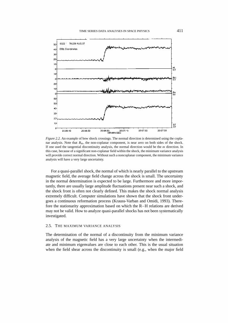
Figure 2.2.An example of bow shock crossings. The normal direction is determined using the copla-nar analysis. Note thatBm, the non-coplanar component, is near zero on both sides of the shock.If one used the tangential discontinuity analysis, the normal direction would be them direction. Inthis case, because of a significant non-coplanar field within the shock, the minimum variance analysiswill provide correct normal direction. Without such a noncoplanar component, the minimum varianceanalysis will have a very large uncertainty.
For a quasi-parallel shock, the normal of which is nearly parallel to the upstreammagnetic field, the average field change across the shock is small. The uncertaintyin the normal determination is expected to be large. Furthermore and more impor-tantly, there are usually large amplitude fluctuations present near such a shock, andthe shock front is often not clearly defined. This makes the shock normal analysisextremely difficult. Computer simulations have shown that the shock front under-goes a continuous reformation process (Krauss-Varban and Omidi, 1993). There-fore the stationarity approximation based on which the R–H relations are derivedmay not be valid. How to analyze quasi-parallel shocks has not been systematicallyinvestigated.
2.5. THE MAXIMUM VARIANCE ANALYSIS
The determination of the normal of a discontinuity from the minimum varianceanalysis of the magnetic field has a very large uncertainty when the intermedi-ate and minimum eigenvalues are close to each other. This is the usual situationwhen the field shear across the discontinuity is small (e.g., when the major field

412 P. SONG AND C. T. RUSSELL
change is in its strength) or when the observations cannot resolve the interior ofthe discontinuity either due to low time resolution of the measurements or fastmotion of the discontinuity relative to the spacecraft. In these circumstances, themaximum variance analysis of the electric field may offer a better determinationof the normal. The maximum variance analysis of the electric field is based onthe fact that the electric field is curl free in steady state (see also discussions onEquation (1.3)) or
∇ × E = −∂B∂t= 0 . (2.12a)
Thus,
n×1E = 0 , (2.12b)
namely, the normal is along the electric field change. Analogous to the minimumvariance analysis of the magnetic field, the normal direction of the discontinuity isalong the maximum variance direction of the electric field.
The electric field data for the analysis can be from either direct measurementsof the electric field or the convective electric field derived from the magnetic fieldand plasma velocity measurements according to the frozen-in condition, orE =−v×B. If the electric field measurements are two dimensional, the third componentof the electric field can be obtained from the frozen-in condition, orE · B = 0.
The major uncertainty in this method comes from the temporal variation termsin Equation (1.3). Both unsteadiness of the discontinuity itself and changes of itsmotion relative to the observer will affect the results. In particular in the case ofthe magnetopause, the boundary usually oscillates instead of being in constantmotion. Another important uncertainty comes from the relative motion betweenthe spacecraft and the boundary, even if the motion is steady. From Equation (2.2),one obtains a tangential electric field change in the spacecraft frame,1ET =Vdisc × (B2 − B1). To remove this effect, one has to transfer the electric fieldinto a frame which is at rest in the discontinuity. However, since the motion of thediscontinuity is in general unknown before the normal direction of the discontinuityis determined, it is difficult to completely remove this effect. Sonnerup et al. (1987)developed a method and gave a comprehensive discussions on how to minimize thiseffect. One way to reduce this effect is as follows.
(1) Find the maximum variance direction of the electric field,n.(2) Measure the average velocity and magnetic field alongn, vn andBn, within
the discontinuity.(3) If the discontinuity is not a shock, calculate
un = ±Bn/√µ0ρ , (2.13)
whereun is similar to the flow velocity across the discontinuity, and we haveassumed that the discontinuity is a rotational discontinuity.
(4) The relative velocity of the discontinuity to the spacecraft is approximately

TIME SERIES DATA ANALYSES IN SPACE PHYSICS 413
Vdisc= νn − un . (2.14)
(5) Subtract the electric field due to the relative motion
E′ = E− Vdisc×B . (2.15)
(6) UsingE′ as corrected electric field, repeat the procedures above, untilndoes not change.
Another source of uncertainty in the maximum variance method is due to theassumption of the frozen-in condition to calculate the electric field if it is not mea-sured directly in three dimensions. Under the frozen-in approximation the effectsdue to the Hall term, the resistivity term, electron pressure gradient term and elec-tron inertial term in Ohm’s law have been ignored. These effects may be importantin sharp changes within a discontinuity.
The principles to evaluate a result of the maximum variance analysis is similarto some of that for the minimum variance analysis discussed in Section 2.2. Thesuccess of the method requires a much larger maximum eigenvalue than the othertwo eigenvalues. The continuity of the normal component of the magnetic fieldand tangential electric field can be used as a check on the results. The maximumvariance analysis does not require many data points within a discontinuity, a sig-nificant advantage over the minimum variance analysis. However, since the plasmavelocity measurements have usually a lower time resolution than the magnetic fieldmeasurements, fewer data points are obtained within and near a discontinuity. If thefluctuations near the discontinuity are not small, the result may be very sensitive tothe number of the data points used in the analysis.
In summary, the maximum variance analysis of the electric field can be used asan alternative in cases when the minimum variance analysis has a large uncertainty.It should be used with caution.
2.6. DEHOFFMANN–TELLER FRAME AND WALEN RELATION TEST
The deHoffmann–Teller (HT) frame is one of the shock frames, ie., a frame atrest in the discontinuity. Here we recall that frames at rest in the discontinuity canhave different tangential velocities. The HT frame moves along the shock frontwith a velocity such that the magnetic field and velocity are parallel, and hence thetangential electric field vanishes (see a brief review by Sonnerup et al., 1995). TheHT frame moves at a speed
VHT = Vi ± Biuin
Bn(i = 1,2) , (2.16)
relative to to the observer. The plus and minus signs correspond to the normalcomponent of the velocity and magnetic field to be antiparallel and parallel, respec-tively. In the normal incidence case, becauseV1T = 0, the downstream tangentialvelocityV2T = (B2T u2−B1T u1)/Bn is in general nonzero. The flow is accelerated

414 P. SONG AND C. T. RUSSELL
Figure 2.3.In the most advanced development (Sonnerup et al., 1987), the acceleration of the HTframe can be introduced to improve the fit and hence the temporal variations of the HT frame can bepartially resolved.
tangentially in crossing the shock due to the kink force of the field. Since theelectric field in the HT frame is zero, the electric field in the spacecraft frameis
Ei = −VHT × Bi . (2.17)
The proportionality between the electric and the magnetic field variations can beused to determine the velocity of the HT frame. Practice indicates that a well-determined HT frame can often be found in the magnetopause (Sonnerup et al.,1990; Walthour et al., 1993). Since the HT frame is a shock frame (VHTn = Vdisc),it can be used to solve the difficulty in determination of a shock frame discussed inSection 2.5. However, in general, since the normal direction is unknown, it needsiteration before a satisfictory result is reached. In its most developed form, usingthe information from the maximum variance analysis of the magnetic and electricfields and the minimum variance analysis ofVHT, through iteration, one can derivenot only the normal direction, but also the normal velocity and its acceleration, seeFigure 2.3, for example. The effect of the acceleration is important as seen in thelast term of Equation (1.3).
Equation (2.17) can also be written in the form of finite field perturbations. Ifthe magnetic field change is in theL direction, and when the discontinuity has nomotion in the normal direction, the electric field change is in theN direction, the

TIME SERIES DATA ANALYSES IN SPACE PHYSICS 415
HT frame moves mainly along theM direction. To deriveVHT in Equation (2.17) isequivalent to a three-parameter fit or a minimum variance problem. Sonnerup et al.(1987) provided the expression for the covariance matrix. Here we should note thatunlessBi andVi outside the shock ramp are not coplanar,VHT and the magneticfields are all in a plane orthogonal to the shock surface. The derived electric fieldchange is along the shock surface and not along the normal direction.
For RDs, combination of Equations (2.5), (2.9), and (2.16) yields the Walenrelation in the spacecraft frame,
V = VHT ± CA , (2.18)
whereCA = B/√µ0ρ for an isotropic plasma andCA = √ξ0B/
√µ0ρ for an
anisotropic plasma,ξ0 = µ0(P⊥ − P‖)/B2 is the anisotropy factor (Chao, 1970),andP⊥ andP‖ are the pressures perpendicular and parallel to the magnetic field,respectively. The plus and minus signs denote the RDs propagate antiparallel andparallel to the magnetic field, respectively. The subscripti has been neglectedassuming that the relationship applies to every measurement.
The Walen relation is a more restrictive test for a discontinuity. It requires notonly a well determined HT frame but also that the discontinuity propagates withthe Alfven speed relative to the flow. A postive result of the test verifies the discon-tinuity to be an RD. Here we should emphasize that a linear relationship betweenthe plasma velocity and magnetic field (or the Alfvén velocity) variations does notnecessarily imply the discontinuity to be an RD unless the offset between the two,VHT (see Equation (2.16)) equals the proportional factor between the electric andmagnetic field variations (see Equation (2.17)).
2.7. SUGGESTED PROCEDURES FOR DISCONTINUITY ANALYSIS
As discussed in Sections 2.2 to 2.4, the three methods commonly used for discon-tinuity analyses are for different purposes. None is intrinsically better than others.However, different methods may provide different normal directions. For example,the noncoplanar direction in the coplanarity analysis is very close to the normaldirection in the tangential discontinuity analysis for the same discontinuity (seeFigure 2.2 for an example). The minimum variance direction could be the non-coplanar direction of a shock. Thus, the question is how to analyze a discontinuitywithout a presumption about its type. The following is a suggested approach.
(1) Collect as much information as possible for the interesting discontinuityin addition to the magnetic field, such as plasma measurements and the measure-ments from other close spacecraft if there are any. These measurements may helpto constrain the results.
(2) Make an overview of the discontinuity to decide where are the upstreamand downstream regions and which major change is most interesting. There maybe more than one choice. Keep in mind that a single discontinuity, when its in-ternal structure can be resolved, may appear to consist of more than one sharp

416 P. SONG AND C. T. RUSSELL
changes, that a discontinuity can oscillate back and forth, and that two distinctdiscontinuities could be very close to each other in time series records.
(3) Begin the analysis by using the minimum variance analysis with cau-tion as discussed in Section 2.2. For low time resolution measurements or whenthe discontinuity being studied moves fast relative to the spacecraft, there maybe no measurement within the discontinuity. In this case, the minimum variancemethod can provide only the direction of maximum variance and the normal of thediscontinuity cannot be determined with only magnetic field measurements.
This step only provides hints to the nature of the discontinuity. One may onlyguess the nature of the discontinuity from the results of the minimum varianceanalysis. For example, if the field in the minimum variance direction is close tozero, the discontinuity may be a tangential discontinuity. If the field in the min-imum variance direction is not small and the field strength is similar on the twosides of the discontinuity, the discontinuity may be a rotational discontinuity. If themajor field change is in only one component and the field strength changes, thediscontinuity may be a shock.
Further determinations of the properties of the discontinuity need plasma mea-surements or assumptions.
(4) Make assumptions of the nature of the discontinuity if the processes as-sociated with the discontinuity are known. In many of discontinuity studies, thenature of the discontinuity has been carefully studied previously with particle mea-surements and hence known, but the plasma moments are not available. In thesecases, assumptions of the nature of a discontinuity can be made, but keep in mindthat the results are conditional depending on the accuracy of the assumptions. Formost of bow shock studies, coplanarity is a good assumption. In fact, most ofthese studies skip step 3 and use the coplanarity analysis directly. In most circum-stances, the magnetopause can be considered as either a tangential discontinuity ora rotational discontinuity. Thus one may try the tangential discontinuity analysisif the minimum variance component is close to zero. The neutral sheet can beconsidered as a rotational discontinuity. However, to analyze the neutral sheetusing the minimum variance method is difficult because the variance in one ofthe tangential components(y) can be very small. The field aligned current sheetsin the low beta magnetosphere can often be treated as tangential discontinuities.For most interplanetary discontinuities, since their natures are unknown withoutplasma measurements, an analysis using only magnetic field measurements cannotbe conclusive except if the field strength remains nearly constant across the discon-tinuity. In this latter case, the discontinuity can be either a tangential discontinuityor a rotational discontinuity and can be treated similarly to the magnetopause situ-ation just discussed above. However, because often an interplanetary discontinuitymoves with a speed similar to that of the solar wind, the flow velocity relative tothe discontinuity is not easy to resolve. Caution should be taken when interpretingit as either a TD or an RD. The main difficulty in analyzing an interplanetary

TIME SERIES DATA ANALYSES IN SPACE PHYSICS 417
discontinuity is the lower time resolution of the data caused by the fast passageof the discontinuity.
With an assumption of the type of a discontinuity, one can determine the normaldirection of the discontinuity using the methods discussed in previous subsections.
(5) Use plasma measurements. With plasma measurements, if the normal direc-tion of the discontinuity has been determined in the last step, the normal velocityof the discontinuity can be determined, according to Equations (2.1) and (2.7),
Vdisc= ρ1V1n − ρ2V2n
ρ1− ρ2. (2.19)
If the plasma velocity measurements are not three dimensional, an additional as-sumption has to be made, hence more uncertainties are introduced, in the cal-culations. Although this relationship is widely used, we would like to point outthat whenVdisc is much less than bothV1n andV2n, it could be in the range ofthe uncertainty of the velocity measurements. In this case, Equation (2.19) is notuseful. The uncertainty in this calculation comes from these major sources. Thefirst is in the direction of the normal. This error is discussed above. The second isthe fluctuations upstream and downstream. In some cases, this source may not beimportant. The third is due to the change in the calibration factor of the instrumentassociated with the change of plasma state as discussed in Section 1.3.3. Whilevelocity measurements, at least of the solar wind ions are usually quite accurate,the plasma density upon which Equation (2.19) depends are not so accurate. If thetemperature and speed of the plasma remain similar across the discontinuity, thissecond source may not be important. Unfortunately under these circumstances, thedensity change is small, leading to a very large uncertainty in the denominatorof Equation (2.19). At shocks, both the temperature and speed vary across thediscontinuity in such a way that the density calibration in some instruments canbe drastically affected (Petrinec and Russell, 1993). An example of where thiscalibration change may have seriously affected measurements across the bow shockcan be found in Lepidi et al. (1996).
For interplanetary discontinuities, plasma measurements can help to determinethe type of a discontinuity. As discussed in step 4, its type can be determinedwhen there is no change in the field strength across the discontinuity. If there isa change in the field strength, in the simplest case, the discontinuity is either atangential discontinuity or a shock. (If the plasma is anisotropic, even an RD canbe accompanied by a change in field strength.) As discussed before, the minimumvariance method has a large uncertainty in these two situations, and the tangentialdiscontinuity analysis and the coplanarity analysis provide two orthogonal normaldirections. Which of these two normals is correct? For a tangential discontinuity,sinceu1n = u2n = 0, orV1n = V2n = Vdisc, the velocity differenceV1− V2 is tan-gential to the discontinuity. Thus, comparing the direction of the velocity differencewith the two normals may eliminate one of the two. There is a possibility that thethree vectors are orthogonal to each other. Another way to distinguish a tangential

418 P. SONG AND C. T. RUSSELL
discontinuity from a shock is to check the total pressure, the sum of the thermalpressure and the magnetic pressureB2/2µo. For a tangential discontinuity, sinceun = Bn = 0, from Equation (2.4), the total pressure remains constant across thediscontinuity. However, this method relies on a good intercalibration between themagnetic field measurements and the plasma measurements. For slow shocks, sincethe change in the total pressure is expected to be small, it is difficult to eliminatethe possibility of slow shocks solely based on the total pressure balance.
(6) Use the timing difference from two spacecraft. Measurements from twospatially separated spacecraft may be able to determine the velocity of a discon-tinuity. If the separation of the two spacecraft along the discontinuity is smallerthan the curvature of the discontinuity and the time scale of the variations of thediscontinuity is much larger than the time scale of the time delay between theencounters of the discontinuity by the two spacecraft (the determination of thetime delay will be discussed in Section 4.1), the discontinuity can be considered asa stationary planar wave front. The curvature of the discontinuity can be determinedby comparing the two normals from the two spacecraft if only a single crossing isobserved by each of them. The velocity of the discontinuity in the plasma framecan be obtained by
Vdisc= L · n1t− V(1,2) cosη(1,2) , (2.20)
whereL ,1t , andη are the separation vector between the two spacecraft, the timedelay between the observations of the discontinuity from the two spacecraft and theangle between the flow velocity, either upstream or downstream, and the normal ofthe discontinuity. Note that Equation (2.20) requires both 3-D plasma measure-ments and the normal direction. Therefore, this step is not independent of the lasttwo steps. It provides additional information and can be used in combination withthe last two steps or as a verification of the results from the last two steps.
2.8. R–HRELATIONS TEST
In the previous steps, we have used two of the R–H relations, the mass conser-vation and the continuity of the normal field. These two relations have the leastuncertainty in practice. However, in steps 4 and 5, to determine the normal ofa discontinuity, we have approximated it by a simplified discontinuity. In fact,a discontinuity may not be any of these simple discontinuities assumed rather acombination of them. Also, an analysis may provide many different parameter setsas the result of multiple interval selections. One should use these parameter sets totest other R–H relations. With this step, one may find the best parameter set forthe study and estimate the uncertainty of the analysis. The uncertainty is the ratioof the difference to the average of the quantity, Equation (2.8), in each of the R–H relations. The conclusions of any analysis should be drawn consistent with thisuncertainty.

TIME SERIES DATA ANALYSES IN SPACE PHYSICS 419
In the procedure described above, the determination of the shock speed car-ries enomous weight in determining the nature of a discontinuity. As discussed inSection 1.3.3, the calibration factor of plasma measurements may change across ashock. To accurately determine the shock velocity is extremely difficult. To solvethis problem, Chao et al. (1995) recently developed a method to derive the prop-erties of a shock without predetermining the shock velocity and then derive theshock velocity afterward. In their method, the R–H relations are combined andwritten in normalized parameters, such as ratios of upstream and downstream val-ues, angles, plasma betas, and Mach numbers. It is realized that to determine anisotropic shock requires only any three independent such parameters. Therefore,one can choose three observationally best determined parameters to substitute intothe normalized R–H relations and then derive those remaining. We suggest usingthe ratio of the ratio of the magnetic field strengths,B2/B1, the upstream shockangle and downstream plasma beta. All these three parameters are independent offrame reference. The ratio of the magnetic field strengths has little uncertainty. Theshock angle depends only on the accuracy of the shock normal determination. Asshown in Figure 1.2, among three plasma moments, the uncertainty in the pressuremeasurements is least and is even smaller for higher temperature plasmas. Thusthe downstream plasma beta is the most accurately measured quantity although itsabsolute calibration needs to be verified.
An interesting finding by Chao et al. (1995) from a parametrical study is thatthe ratio of the upstream and downstream plasma densities is less sensitive thanthe ratio of plasma velocities. In other words, a small difference in the densityratio corresponds to a large range of shock parameters. A small uncertainty inthe density measurements will hence cause drastically different conclusions aboutthe shock properties. Such temperature and velocity dependences of the densitycalibration of several plasma instruments as found by Petrinec and Russell (1993)would cause such uncertainties across almost any shock crossing. Therefore, it isnot recommended to use the density ratio as a primary parameter in shock normaldetermination unless the density calibration on both sides of the shock is wellknown.
Chao (1995) shows that in many cases, the parameters derived using the best fitto all R–H relations are actually far from possible solutions of the R–H relations.This result indicates that because of the complicated relationship among differentvariables, the values of the unmeasured quantities determined from a best fit ac-tually do not represent well the real values of these quantities for each set of theparameters at a given point. It is not recommended to use a best fit of all R–Hrelations.
In summary, using only magnetic field measurements one can determine thenormal direction of a discontinuity in simple cases. The minimum variance methodapplies only if there are measurements within a discontinuity. It has a large uncer-tainty for either a tangential discontinuity or a shock. The tangential discontinuityand coplanarity analyses impose strong assumptions on the type of a discontinuity.

420 P. SONG AND C. T. RUSSELL
They should be used carefully in combination with the minimum variance analysisand plasma measurements.
3. Wave Analyses
Wave analyses are used to determine the properties and characteristics of waves,such as propagation direction, wave frequency, wave amplitude, polarization, andmode. With measurements at multiple locations one can determine the phase speed,wave number, and etc. The waves of concern here are at frequencies near or lowerthan the ion gyrofrequency, or so-called ULF (Ultra Low Frequency) waves, mea-sured in the spacecraft frame. Waves of higher frequencies will be discussed brieflyin Section 3.6. We will focus on electromagnetic waves with emphasis on MHDwaves. Methods for wave analysis based solely on the magnetic field measure-ments have been well developed and will be discussed as routine procedures inSection 3.2. From measurements at a single site these analyses can provide onlythe propagation direction (with an ambiguity in sign) and wave parameters in thespacecraft frame. To resolve the Doppler shift and to determine the direction ofpropagation, one needs to either use more than one satellite and plasma measure-ments or to make assumptions on the mode of the wave and use the dispersionrelation calculated from theory as an accurate description of the wave. We notethat dispersion relations developed for small amplitude linear waves may not beaccurate for the large amplitude waves encountered in space. Also dispersion rela-tions that ignore the interaction with the gyro and thermal motions, such as in theHall-MHD treatment, may be inaccurate in the moderate and high beta collision-free plasmas in space. Related issues are discussed in Section 3.3. To identifythe mode of a perturbation is crucial to understand the underlying physics of theprocesses that generate the wave. Several schemes to make the identification havebeen developed in recent years and will be discussed in Section 3.4.
3.1. BACKGROUND
The most powerful tool in general use for wave analyses is the Fourier analysis. Itsprinciples can be found in most time-series data-analysis textbooks. However, inspace physics, we deal with Fourier analysis of vectors. For a wave the perturba-tions in different components of a vector are correlated. This relationship definesa covariance matrix in the frequency domain, or the so-called spectral matrix. ThePrincipal Axis Analysis can be used to analyze the covariance matrix in much thesame way as it is used above in the time domain analysis (McPherron et al., 1972).Fourier analysis, the resultant spectral matrix, and the Principal Axis Analysis formthe main ingredients of the most popular wave analysis technique for waves inspace plasmas.

TIME SERIES DATA ANALYSES IN SPACE PHYSICS 421
3.1.1. ApproximationsMost of the existing wave analysis techniques in the time domain are based on theassumption that there is one dominant wave being analyzed. Most time series arisefrom a combination of many waves from various sources. If the coupling amongdifferent coexisting waves is weak, the analysis can be performed in the frequencydomain. Spectral analysis transforms the time series into a simple superpositionof waves of different frequencies. Usually when we analyze a wave we treat afinite band of frequencies, i.e., several successive Fourier amplitudes are groupedtogether. At each of the individual frequencies there is an amplitude and a phase,or a cosine (in phase) and a sine (quadrature phase) amplitudes. If there is a singlesource of all the wave amplitudes seen in this band, then the ratios of the ampli-tudes seen in two different components of the magnetic field over the band willbe fixed (but not necessarily the amplitudes themselves) this quality is measuredby the parameter called coherence which varies from zero to unity. In practice arandom signal has a non-zero coherence whose value is determined by the numberof Fourier estimates in the band analyzed.
Many magnetospheric waves appear with clear sinusoidal patterns, however,they may not be propagating but standing, in the sense they are the sum of twowaves propagating in opposite directions with nodes in the ionosphere. For thesewaves, the Fourier analysis to be discussed in the following is applicable, but thematrix analysis is not. We note that there is another type of standing wave, onein which the wave propagation velocity is exactly balanced by the plasma bulkvelocity so that the wave train stays fixed relative to its source. Such waves canbe analyzed with the matrix method if the motion of the spacecraft or the sourcecarries the observer through the wave train. We note further that the special prop-erty of the whistler mode that the group velocity exceeds the phase velocity allowsenergy to be pumped into a phase standing wave.
If the amplitude of the fluctuations is large, the harmonic generation associ-ated with the nonlinear effects will affect the analysis. We discuss this issue inSection 3.5.
3.1.2. An Ideal WaveThe magnetic field vector can usually be measured relatively easily with adequateaccuracy and time resolution. Moreover, it carries most of the Poynting flux inelectromagnetic waves in plasmas of interest to us. (Here we recall that the ratioof the electric to magnetic energies for an electromagnetic wave equals the ratioof the phase velocity to the speed of light.) Thus it is often used to model wavefluctuations. The magnetic vector for a monochromatic plane wave propagating inthez direction is
Bx = Bx0+ δBx exp [−i(ωt − k · r)] ,By = By0+ δBy exp [−i(ωt − k · r + φ)] , (3.1)

422 P. SONG AND C. T. RUSSELL
Bz = Bz0 ,where subscript 0 and prefixδ denote the average and deviation from the average,respectively, andω, k, r andφ are the frequency, wave number, spatial vector, andthe phase, respectively. Since∇ · B = 0, k · δB = 0 for plane waves and thereforeδBz = 0. This is a most important feature in wave analyses. The power spectralmatrix is
P(ω) =
δB2
x δBxδByeiφ 0
δBxδBye−iφ δB2
y 0
0 0 0
, (3.2)
wherePij (ω) = Bi(ω)B∗j (ω); i, j,= x, y, z; andBi(ω) is the Fourier transformof Bi(t). The asterisk denotes the corresponding complex conjugate.
In general, the off-diagonal elements can be written as a real part plus an imag-inary part. The real (imaginary) part corresponds to the component of whichδBiandδBj are in or 180◦ out of phase (of phase shift of±90◦).
The intensity of the wave is defined as
I (ω) = TrP(ω) = δB2x + δB2
y (3.3a)
and the ellipticity (Rankin and Kurtz, 1970)
ε = tanψ , (3.4a)
where
sin 2ψ = 2 Im(Pxy)
[(TrPxy)2− 4 |Pxy |]1/2and Pxy is the 2× 2 subtensor ofP. For a linearly polarized wave,φ = 0 orπ, ε = 0. For a circularly polarized wave,φ = ±1
2π , δBx = δBy andε = ±1,where the plus sign is for right-hand polarization and the minus sign is for left-handpolarization.
3.1.3. Spectral AnalysisFor a given interval, the spectral matrixP(ω) can be evaluated for a selectedfrequency range,1ω. In general the matrix can be written as
P = Re(Pij )+ i Im(Pij ) . (3.5)
Its real part is symmetric, and its imaginary part is antisymmetric and consists ofonly off-diagonal elements because the covariance matrix is Hermitian. The realpart can be diagonalized using the Principal Axis Analysis (see Section 1.4). Inprincipal axis coordinates, the matrix is

TIME SERIES DATA ANALYSES IN SPACE PHYSICS 423
P′ =
λ1
λ2
λ3
+ i Im
0 P ′xy P ′xz
−P ′xy 0 P ′yz
−P ′xz −P ′yz 0
, (3.6)
whereλ1 > λ2 > λ3 and are real. The matrix for isotropic noise is
Pnoise= α
1
1
1
. (3.7)
Comparing the above expressions with Equation (3.2), one finds thatλ3 corre-sponds to the noise in thek direction. The wave intensity should then be defined,if the noise is isotropic, as,
I = λ1+ λ2− 2λ3 . (3.3b)
As we discussed in Section 3.1.2, each imaginary element gives the correlationof the fractions of the two corresponding components that have±90◦ phase shift.Im (Pij )
′ should be equal to or less than√λiλj . If k is alongz′, Im P ′xz and ImP ′yz
should be very small. For a purely elliptically polarized wave with isotropic noise,Im P ′xy =
√(λ1− λ3)(λ2− λ3), and
√λ1− λ3 and
√λ2− λ3 are the lengths of the
major and minor axes of the polarization ellipse, respectively. For a nearly linearlypolarized wave,λ2 ≈ λ3. The ellipticity is
|ε| =√λ2− λ3
λ1− λ3(3.4b)
and its sign is the same as of ImP ′xy . The sense of the polarization is determined bythe sign of ImP ′xy (right hand for plus and left hand for minus). The amplitude ofthe wave can then be defined as
a =√
I
1+ ε2. (3.8a)
A linearly polarized wave can be decomposed as two circularly, but with oppo-site senses, polarized waves. An elliptical polarized wave can also be decomposedinto two circularly polarized waves with opposite senses but different amplitudes.Therefore, every wave has left-hand and right-hand components. One can showthat the amplitudes of the right- and left-hand components are (Kodera et al., 1977)
aRL= (λ1− λ3)± ImP ′xy
2√λ1− λ3
=√λ1− λ3
2(1± ε) . (3.8b)

424 P. SONG AND C. T. RUSSELL
3.2. ROUTINE WAVE ANALYSIS
In practice a time series of data usually contains some flags and gaps. Before anywave analysis, one has to remove these flags and fill the gaps. Sometimes, spikes inthe data can be considered as flags if their time scale is much much smaller than theperiod of the wave being studied. In general, deflagging reduces the wave powerat higher frequencies and degapping adds wave power to low frequencies. Someinstruments are operated periodically leaving periodic gaps in the data. The gapswill create false wave power in the corresponding periods. After the preparation ofthe data, one is ready for the routine wave analysis.
3.2.1. Coordinate SystemA wave can be analyzed more easily by choosing a proper coordinate system. Sinceone way to characterize a wave is to see if the wave is compressional or transverse,we suggest the use of field-aligned coordinates as discussed in Section 1.2.2. In thiscoordinate system, if the perturbations are mainly along the background magneticfield direction, the wave is compressional, otherwise it is transverse.
Assume in magnetic field coordinates the field direction asz. In generalthe spectral matrix is not diagonal,Pzz is the compressional power andPxx + Pyyis the power transverse to the field. The real part of an off-diagonal elementRePij /
√PiiPjj gives the portion of which the two components are in phase (when
positive) or 180◦ out of phase (when negative). Note hereij satisfies the right-handrule, otherwise a minus sign needs to be added. Similarly, ImPij /
√PiiPjj gives
the portion of the signals that are±90◦ out of phase. The properties of a wave canbe decided by careful examination of each element of the spectral matrix as will bediscussed in Sections 3.2.3 to 3.2.6.
3.2.2. DetrendingMost wave analysis methods essentially perform Fourier analysis on a segment ofa time series data. A critical but implicit assumption of Fourier analysis is that thetime series is periodic. Thus a slow trend in the signal is transformed into a saw-tooth variation by the Fourier analysis technique. Figure 3.1 shows the effects ofvarious detrending methods on subsequent Fourier analysis. The top line shows theFourier spectra of linear, quadratic or cubic trends of the field increasing from zeroto one nanotesla. The spectra for the three trends are almost identical. The slope isabout−2. This slope will have a profound effect on studying the slopes of spectraas discussed in Section 3.2.3. The corresponding amplitude can be as large as 10%in the low frequency range and decreases one order for every two-order increasein frequency. A non-zero average of a constant signal has only minimal effects onthe spectral analysis as shown in the lowest line in Figure 3.1. A linear detrendingcan remove a linear trend completely and lower the effects down to the level ofthe non-zero average trace shown. Similarly quadratic detrending will remove thepower due to the quadratic trend. A linear detrending is effective to reduce the error
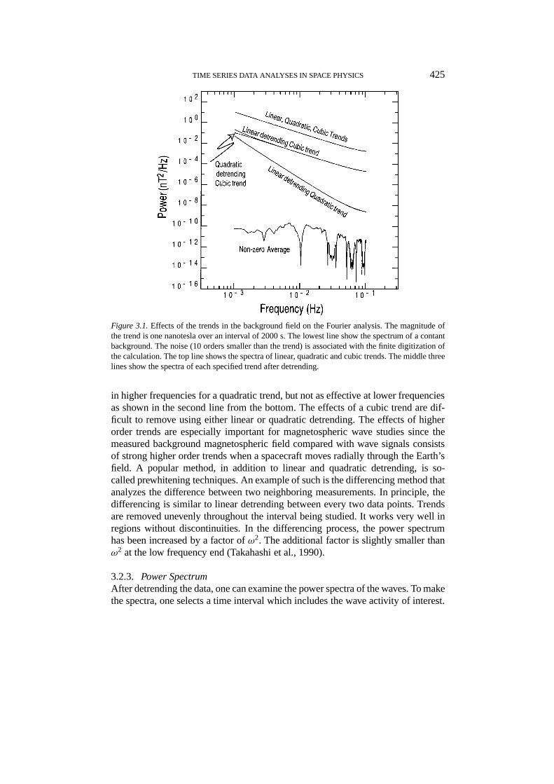
TIME SERIES DATA ANALYSES IN SPACE PHYSICS 425
Figure 3.1.Effects of the trends in the background field on the Fourier analysis. The magnitude ofthe trend is one nanotesla over an interval of 2000 s. The lowest line show the spectrum of a contantbackground. The noise (10 orders smaller than the trend) is associated with the finite digitization ofthe calculation. The top line shows the spectra of linear, quadratic and cubic trends. The middle threelines show the spectra of each specified trend after detrending.
in higher frequencies for a quadratic trend, but not as effective at lower frequenciesas shown in the second line from the bottom. The effects of a cubic trend are dif-ficult to remove using either linear or quadratic detrending. The effects of higherorder trends are especially important for magnetospheric wave studies since themeasured background magnetospheric field compared with wave signals consistsof strong higher order trends when a spacecraft moves radially through the Earth’sfield. A popular method, in addition to linear and quadratic detrending, is so-called prewhitening techniques. An example of such is the differencing method thatanalyzes the difference between two neighboring measurements. In principle, thedifferencing is similar to linear detrending between every two data points. Trendsare removed unevenly throughout the interval being studied. It works very well inregions without discontinuities. In the differencing process, the power spectrumhas been increased by a factor ofω2. The additional factor is slightly smaller thanω2 at the low frequency end (Takahashi et al., 1990).
3.2.3. Power SpectrumAfter detrending the data, one can examine the power spectra of the waves. To makethe spectra, one selects a time interval which includes the wave activity of interest.
426 P. SONG AND C. T. RUSSELL
Observed waves often are not perfectly sinusoidal for a long period. How manywave cycles should be included for an analysis? The longest period in a Fourierspectrum is determined by the length of the selected interval. If only one wave cycleis selected, one would not obtain a meaningful peak in the spectrum. Furthermore,any residual trend in the background will strongly affect the analysis. It is commonpractice to select an interval containing at least five to six wave cycles in orderto derive a statistically significant result. The more wave cycles are included, thebetter are its statistics, but the more chance has one to include waves of differentsources or effects of source variation.
The spectrum can be spiky. To enhance the robustness of the result, one canaverage several Fourier estimates. The number of the total Fourier estimates inthe average is called ‘bandwidth’. Increasing the bandwidth improves statisticalsignificance of the spectrum, reduces the resolution of frequency, and increases thelower-cutoff frequency of the spectrum.
To examine power spectra, firstly one may compare the power in the frequencyrange of interest for the different components and the strength of the field. Usually,the power for one or two components is much higher than that for the others. Todetermine whether a wave is compressional or transverse one can compare thepower in the strength of the fieldPt (the compressional component) withPx+Py+Pz−Pt (the transverse component) wherePx, Py , andPz are powers inBx,By, andBz, respectively.
Secondly, one may look for peaks in the spectra. A sharp peak indicates thatthe wave is nearly monochromatic and a resonance of some sort may occur in theprocess being studied. However, if a sharp peak occurs exactly at the frequencyof the spin of the spacecraft or at some multiple, it may be caused by an imper-fect despinning process. Usually the spin tone occurs only in the two transversecomponents to the spin axis and usually little in the field strength. A broad peakmay indicate that many wave modes contribute to the wave. If the plasma is not in arapid motion, or the Doppler shift is small (see detailed discussions in Section 3.3),one may compare the peak frequency with the characteristic frequencies of theplasma, such as the gyrofrequencies. If the wave frequency is much smaller thanthe ion gyrofrequency, the wave is usually referred to, rightly or wrongly, as anMHD wave. If the wave frequency is near the ion gyrofrequency, the wave maybe associated with ion gyromotion. Sometimes the trough between two peaks maybe also of interest since it may be associated with resonant absorption by particles(Young et al., 1981; Anderson et al., 1991). Thus a trough could occur at a localcharacteristic frequency for certain species.
Thirdly, one may examine the slope of the spectrum (LaBelle and Treumann,1988). The slope may provide some information about cascading processes in thefrequency domain. Cascading processes describe the evolution of wave power inwave number. A wave cycle may break into two wave cycles with smaller wave-lengths or two wave cycles may coalesce to form one wave cycle with a longerwavelength. If this process continues, a single wave mode may evolve into a spec-

TIME SERIES DATA ANALYSES IN SPACE PHYSICS 427
trum with many wave numbers. However, we should point out that to compare themeasured slopes with those given by theory is not as straight forward as many peo-ple thought. The cascading processes are described in the wave number domain inalmost all theoretical work. They may appear differently in the frequency domain.In interplanetary space, since the solar wind velocity is much greater than the phasevelocity for MHD waves, the measured spectrum is essentially due to the Dopplershift and hence is proportional to that of the wave number. Thus, a power spectrumin the frequency domain can be converted linearly into the wave number domainif the waves at different frequencies propagate in the same direction (which needsto be demonstrated), and is easily used in theoretical investigations. In other cases,the conversion from the frequency domain to the wave number domain may notbe linear due to the dispersion. The slope of the power spectrum in the frequencydomain may not be purely due to cascading. We should point out that an imperfectdetrending process will strongly affect the analysis of the slope of a spectrum. Oneway to check this is to examine whether the amplitude in the lower frequency endis significantly smaller than a few percent of the trend in the background field.
3.2.4. CoherenceIn any region in space several wave modes may coexist. Each mode has a particularpolarization at a particular frequency. When we observe these waves we measurethe sum of the wave modes and the noise of the observing system. One way toseparate these wave modes is to check the cross correlations between differentcomponents as a function of frequency. Coherence analysis is a particular way ofusing the cross-correlations, i.e., the off-diagonal elements in Equation (3.5). Thecoherence is defined as the square-root of|Pij |2/(PiiPjj ). (See also Section 4.2).In the coordinate system of the waves, for a purely compressional wave, the fieldaligned component should have little coherence with the two transverse compo-nents. On the other hand, for a transverse wave, the two transverse componentsmay have high coherence. Note, however, if one is not performing the analysis inthe coordinate system of the waves so that any wave might excite all three sensorsor directions of analysis, then high coherence could result in high coherence inall these possible pairs of signals. Combining the information gained from thecoherence analysis with that from the power spectra, one may find sometimesthat different peaks in the power spectra correspond to different wave modes. Incoherence analysis, the phase difference between two components may also becalculated,φij = Im Pij /|Im Pij | tan−1(Im Pij /RePij ). From the phase differ-ence between the two transverse components, one may be able to determine thepolarization of a transverse wave. The phase difference can also be used for modeidentification as discussed in Section 3.4.
3.2.5. Propagation DirectionIn principle, there are two methods to determine the propagation directionk. Com-paring Equation (3.6) with (3.2), in analogy of the minimum variance analysis
428 P. SONG AND C. T. RUSSELL
in the discontinuity analysis, one can takek either parallel or antiparallel to theminimum eigenvector. This method is referred to as Born-Wolf method or principalaxis analysis (Born and Wolf, 1965). This method is based on the information con-tained in the real part of the covariance matrix, sometimes called the cospectrum.Its applicability is limited by the ratio ofλ2/λ3 in the same manner as the minimumvariance analysis. An alternative method is based on the information contained inthe imaginary part of the covariance matrix, sometimes called the quaspectrum.Means (1972) shows that the unit vectork0 can be given by
k0x = ±Im P ′yz/IP ,
k0y = ∓Im P ′xz/IP , (3.9)
k0z = ±Im P ′xy/IP ,
whereIP = (Im P ′2xy + Im P ′2xz + Im P ′2yz)1/2, the plus (minus) sign is for right(left)-handed polarization.
The differences between the two methods were studied by Arthur et al. (1976),who suggested that the Born–Wolf method may be better for linear polarizationand the Means method for circular polarization. One advantage of the Meansmethod is that it provides the sense of the polarization.
For a linearly polarized wave, the propagation direction cannot be well deter-mined from the minimum variance analysis. If the waves are mainly compressional,their propagation direction can be determined according to the coplanarity the-orem assuming that they are either fast or slow modes (see more discussion onwave modes in Section 3.3). The coplanarity theorem requires that the backgroundfield, the perturbed field and the wave vector be coplanar for the fast and slowmode waves. Since the perturbed field is perpendicular to the wave vector, thepropagation direction is (Russell et al., 1987)
k‖(1B× B0)×1B , (3.10)
where the direction of the perturbed field,1B, is in the direction of the maximumvariance.
The propagation direction cannot be well determined for nearly linearly polar-ized intermediate mode waves.
3.2.6. Wave PropertiesFrom principal axis analysis of the covariance matrix, one can derive properties ofthe wave such as its amplitude, ellipticity and compressibility using the definitionsgiven in Section 3.1. For a linearly polarized wave the intermediate eigenvalueand minimum eigenvalue may be close to each other, and hence the propagationdirection not well determined. In this case, the direction of the perturbed fieldwhich is the direction of maximum eigenvector is well determined. If the linearly

TIME SERIES DATA ANALYSES IN SPACE PHYSICS 429
polarized wave is compressional (fast or slow mode), the propagation direction canbe determined according to the coplanarity theorem. On the other hand, for a nearlycircularly polarized wave, the maximum eigenvalue is close to the intermediateeigenvalue. In this case, the propagation direction is well determined. If all threeeigenvalues are similar, say the differences are less than an order of magnitude,the fluctuations are turbulent. Neither the propagation direction nor polarizationis well determined. Note that the wave properties are derived for only a selectedfrequency band. When one integrates over the entire frequency range, the resultsgive the average properties over the whole spectrum and should be identical to theresults of principal axis time series analysis. Wave analysis needs the backgroundmagnetic field for referencing the wave polarization. Thus if the wave propertiesare obtained after detrending or filtering, one must make sure that the backgroundfield be made available in the analysis.
3.2.7. FilteringFiltering the time series data can be used to examine the behavior, amplitude forexample, of the wave changing with time or location in space. The interestingissues here are generation or damping of the waves, the nodes of the field lineresonance and wave packets. Filtering may be performed in the time domain or thefrequency domain. In the time domain filters may be symmetric about the pointof interest with identical weights multiplying the data on either side of the centralpoint. Such filters have no phase lag, but have the disadvantage for real time use thatthey look forward in time. Filters can also be recursive using only data previous tothe point in question. Such filters have phase variations with frequency but can beused in real time situations. Filtering can also be done with weighting the powersin the frequency domain. Such a filtering process is accomplished by multiplying afilter function by the Fourier spectrum to be filtered, and then inverting the resultantspectrum back to the time domain. An ideal filter function removes the variationsin the unwanted frequency range while keeping the rest unchanged. However, inreality, this process may either introduce artificial fluctuations into the resultingtime series or leave some residual power in the frequencies to be filtered.
Figure 3.2 shows examples of commonly used filter functions using time do-main weighting. One selects a filter according to the requirements of his/her analy-sis. There are three major concerns in choosing a filter: how close to unity itspass-band is, how close to zero its stop band is and how sharp the cutoff is. Ingeneral, each filter is good in one or two of the three aspects. For example, therectangular window, Figure 3.2(a), has a sharp cutoff, but its stop band is not cleanand it creates artificial waves in the pass band. The Kaiser window, Figure 3.2(c),has the broadest cutoff transition but with the lowest stop band response. The Han-ning window, Figure 3.2(b), is a compromise between the rectangular and Kaiserwindows and is widely used in data analysis. Hamming window, not shown, issimilar to the Hanning window and is also popularly used.

430 P. SONG AND C. T. RUSSELL
Figure 3.2.Response functions of three low-pass filter windows. (a) Rectangular window, (b) Han-ning window, and (c) Kaiser window. The left panels show the linear response and right panels showdecibel response. The Nyquist frequency is 2 Hz and the high-cutoff frequency is 1 Hz.
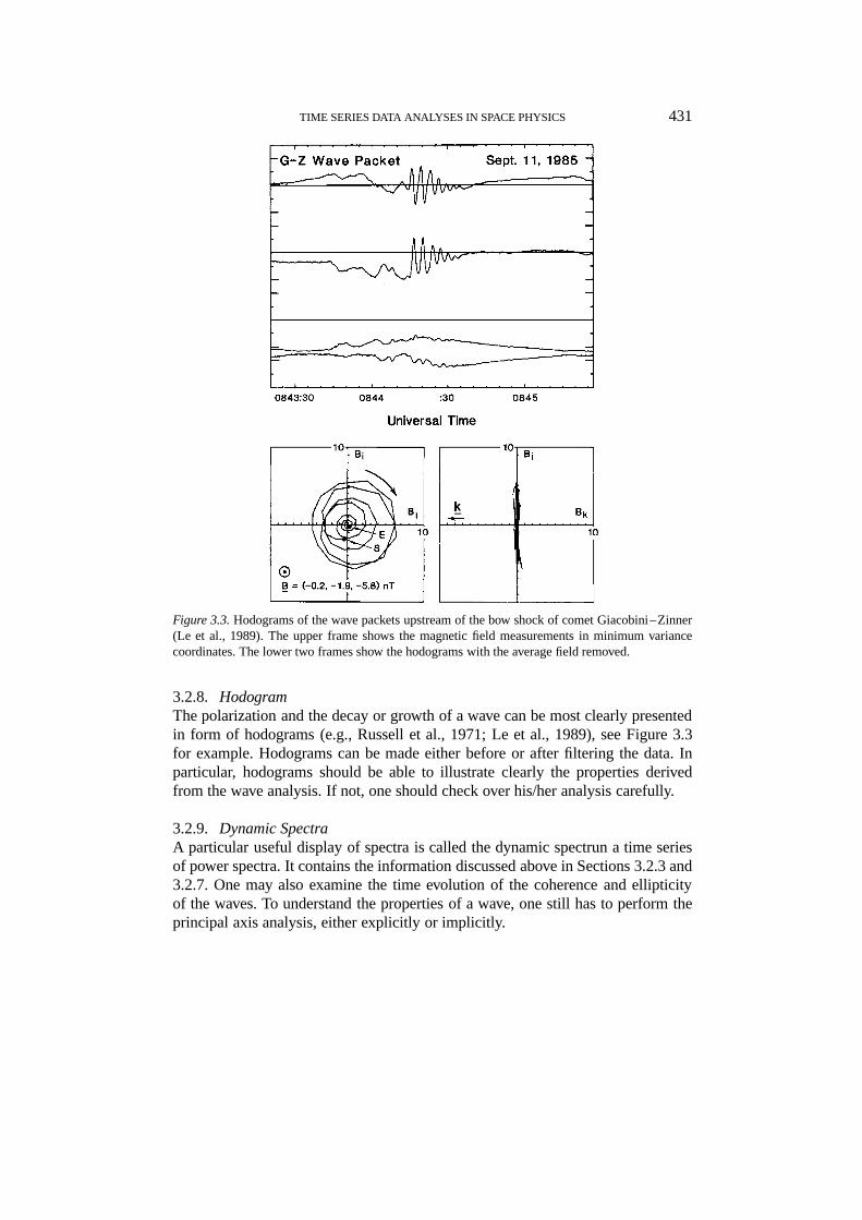
TIME SERIES DATA ANALYSES IN SPACE PHYSICS 431
Figure 3.3.Hodograms of the wave packets upstream of the bow shock of comet Giacobini–Zinner(Le et al., 1989). The upper frame shows the magnetic field measurements in minimum variancecoordinates. The lower two frames show the hodograms with the average field removed.
3.2.8. HodogramThe polarization and the decay or growth of a wave can be most clearly presentedin form of hodograms (e.g., Russell et al., 1971; Le et al., 1989), see Figure 3.3for example. Hodograms can be made either before or after filtering the data. Inparticular, hodograms should be able to illustrate clearly the properties derivedfrom the wave analysis. If not, one should check over his/her analysis carefully.
3.2.9. Dynamic SpectraA particular useful display of spectra is called the dynamic spectrun a time seriesof power spectra. It contains the information discussed above in Sections 3.2.3 and3.2.7. One may also examine the time evolution of the coherence and ellipticityof the waves. To understand the properties of a wave, one still has to perform theprincipal axis analysis, either explicitly or implicitly.
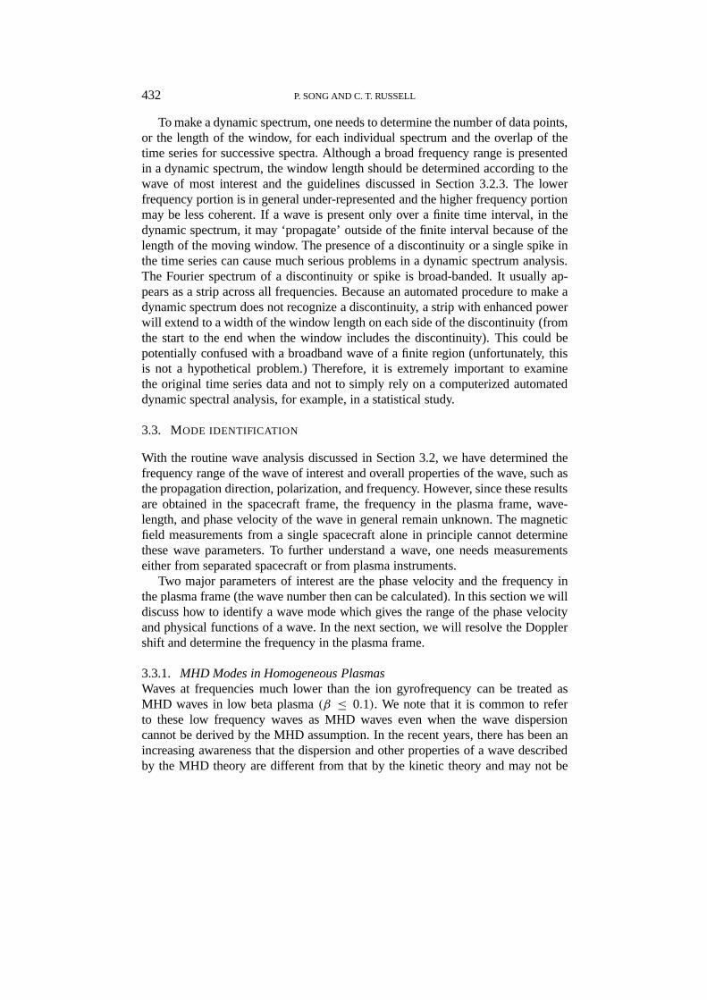
432 P. SONG AND C. T. RUSSELL
To make a dynamic spectrum, one needs to determine the number of data points,or the length of the window, for each individual spectrum and the overlap of thetime series for successive spectra. Although a broad frequency range is presentedin a dynamic spectrum, the window length should be determined according to thewave of most interest and the guidelines discussed in Section 3.2.3. The lowerfrequency portion is in general under-represented and the higher frequency portionmay be less coherent. If a wave is present only over a finite time interval, in thedynamic spectrum, it may ‘propagate’ outside of the finite interval because of thelength of the moving window. The presence of a discontinuity or a single spike inthe time series can cause much serious problems in a dynamic spectrum analysis.The Fourier spectrum of a discontinuity or spike is broad-banded. It usually ap-pears as a strip across all frequencies. Because an automated procedure to make adynamic spectrum does not recognize a discontinuity, a strip with enhanced powerwill extend to a width of the window length on each side of the discontinuity (fromthe start to the end when the window includes the discontinuity). This could bepotentially confused with a broadband wave of a finite region (unfortunately, thisis not a hypothetical problem.) Therefore, it is extremely important to examinethe original time series data and not to simply rely on a computerized automateddynamic spectral analysis, for example, in a statistical study.
3.3. MODE IDENTIFICATION
With the routine wave analysis discussed in Section 3.2, we have determined thefrequency range of the wave of interest and overall properties of the wave, such asthe propagation direction, polarization, and frequency. However, since these resultsare obtained in the spacecraft frame, the frequency in the plasma frame, wave-length, and phase velocity of the wave in general remain unknown. The magneticfield measurements from a single spacecraft alone in principle cannot determinethese wave parameters. To further understand a wave, one needs measurementseither from separated spacecraft or from plasma instruments.
Two major parameters of interest are the phase velocity and the frequency inthe plasma frame (the wave number then can be calculated). In this section we willdiscuss how to identify a wave mode which gives the range of the phase velocityand physical functions of a wave. In the next section, we will resolve the Dopplershift and determine the frequency in the plasma frame.
3.3.1. MHD Modes in Homogeneous PlasmasWaves at frequencies much lower than the ion gyrofrequency can be treated asMHD waves in low beta plasma(β ≤ 0.1). We note that it is common to referto these low frequency waves as MHD waves even when the wave dispersioncannot be derived by the MHD assumption. In the recent years, there has been anincreasing awareness that the dispersion and other properties of a wave describedby the MHD theory are different from that by the kinetic theory and may not be
TIME SERIES DATA ANALYSES IN SPACE PHYSICS 433
appropriate for moderate and high beta plasmas, with which we are often dealingin space. Nevertheless, we base our discussion on MHD theory and point out wherecaution should be taken.
In MHD linear theory for isotropic uniform plasmas, there are four modes,the fast, intermediate, slow and entropy modes (e.g., Kantrowitz and Petschek,1966; Kivelson and Russell, 1995). There is an ongoing debate on the existenceof the MHD slow mode. In linear kinetic theory, the slow mode is strongly Landaudamped in highβ plasmas when the electron temperature is smaller than the iontemperature, as it is in the magnetosheath, plasma sheet and most of the mag-netosphere, and its phase velocity is greater than the intermediate mode velocity(Gary, 1992). However, in data analyses an observation should not eliminate theslow mode from consideration solely on the basis of theory, because conditionsmay exist that maintain this mode in the face of damping. In the following dis-cussion, we will refer to the intermediate mode as the Alfvén mode to avoid theimplication of the ordering in the phase speeds.
The entropy mode is a nonpropagating perturbation with a zero phase velocity.The phase velocities for the other three modes are derived from linear MHD theory,to be,
v2phase(f,s) = 1
2[(C2S+ C2
A)±√(C2
S+ C2A)
2− 4C2SC
2A cos2 θ] , (3.11a)
vphase(a) = CA cosθ , (3.11b)
whereCS, CA, andθ are the sound speed, Alfvén speed and the angle between thewave vector and the background field. The subscriptsf ands stand for the fast andslow modes and correspond to the plus and minus signs on the right-hand-side ofEquation (3.11a). The subscript A stands for the Alfvén mode. Their dependenceon θ andβ = 2C2
S/C2Aγ is given in Figure 3.4.
Characteristic features of each mode can be obtained from the perturbationrelations. The Alfvén mode is incompressible, and thus the perturbations shouldbe transverse. Both fast and slow modes are compressible and hence contain per-turbations in both field pressure and plasma pressure. For the fast (slow) mode,the two pressures vary in (180◦ out of) phase. These characteristics can be easilydifferentiated in the power spectra (see Section 3.2.3) and coherence analysis (seeSection 3.2.4). In inhomogeneous plasmas, the Alfven mode may contain varia-tions in density and the field strength. However, it requires that the variations inthe total pressure, the sum of the thermal and magnetic pressures, be zero. Herewe can see how important it is to have an accurate intercalibration between theplasma and field measurements. Otherwise, an inhomogeneous Alfvén wave maybe misidentified as a homogeneous slow wave, and vice versa. Under this situation,careful examination of the perturbation and propagation directions is extremelyimportant.
The fast mode propagates more isotropically than the other two propagatingmodes. Since the other two modes do not propagate perpendicular to the magnetic

434 P. SONG AND C. T. RUSSELL
Figure 3.4.MHD phase velocities as functions ofβ and field direction. The field direction is alongy.RatioC2
S/C2A equalsγβ/2, quantitiesCA andCS are the Alfven and sound speeds, respectively. The
phase velocity for the entropy mode is zero, i.e., at the origin of each frame.CM is the magnetosonicspeed for perpendicular propagation equal to the square root of the sum of the squares of the Alfvenand sound speeds.
Figure 3.5.Physical functions of the three propagating MHD modes.

TIME SERIES DATA ANALYSES IN SPACE PHYSICS 435
field, the fast mode most efficiently transmits the pressure perpendicular to thefield. The Alfvén mode bends and twists the magnetic field and the plasma motion.The function of the slow mode is more interesting. As shown in Figure 3.5, if oneapplies a pressure perturbation perpendicular to a flux tube, the field strength willincrease to conserve the flux while the cross-section of the tube decreases. If thisis done slowly then, the thermal pressure will decrease because the pressure has achance to equilibrate. Then the thermal pressure is anticorrelated with the magneticfield pressure,B2/2µ0. This is accomplished by the plasma moving away from thecompressed region. Thus the role of the slow mode is to convert the perpendicularpressure perturbations to parallel pressure perturbations. With these physical pic-tures in mind, one can more readily understand why a particular mode exists in acertain region.
3.3.2. Mirror ModeThe mirror mode instability can be derived from the MHD slow mode branchwith inclusion of a finite temperature anisotropy,T⊥/T‖. However, Southwoodand Kivelson (1993) showed that the instability is a result of kinetic effects. Theunstable condition is
T⊥T‖≥ 1+ 1
β⊥, (3.12)
whereβ⊥ is the plasma beta evaluated using the perpendicular temperature. Themirror mode is a purely growing mode with zero frequency in the frame of plasma.It has a maximum growth rate whenk is about 70◦ from the field direction (Gary,1992). The perturbations resulting from the instability convect with the plasmaflow and are observed as oscillating waves. Krauss-Varban et al. (1994) showedthat these perturbations correspond to the entropy mode in MHD. The mirror modeis expected to exist downstream of the bow shock (Crooker and Siscoe, 1977; Leeet al., 1988) and in outer magnetosphere where the plasma condition usually meetsthe mirror instability criterion. The perturbations associated with the mirror modeare similar to that of the perpendicular propagating slow modes. A major differencebetween the two is that the phase velocity is zero for the former but non-zero for thelatter. However, when the slow mode phase velocity is small and the flow velocityis dominant, the two modes are difficult to distinguish as discussed in Section 3.4.The schemes discussed in the next subsection are designed to differentiate the slowand mirror modes.
3.3.3. Transport RatiosOne way to identify a wave mode is to measure the phase velocity and compareit with the expected dispersion relation (Hoppe et al., 1981). However, as will bediscussed in Section 3.4, to measure the phase velocity needs at least two spacecraftand 3-D plasma measurements. A different approach is to determine the modeaccording to the ratios among perturbations of different quantities. These ratios

436 P. SONG AND C. T. RUSSELL
are referred to as transport ratios (e.g., Gary and Winske, 1992). Because of thedifference in the roles of waves, each mode has a particular set of values of thetransport ratios which can be calculated from theory.
3.3.3.1. Transverse ratio. The transverse ratio is defined as the ratio of the trans-verse component of magnetic wave power to the compressional component power,or
TR = δB⊥ · δB⊥/δB2‖ (3.13)
whereδB⊥ · δB⊥ = δB · δB− δB2‖ , andδB‖ is the amplitude in the magnetic field
strength. WhenTR � 1, the wave is transversely polarized and whenTR � 1,compressionally polarized.
3.3.3.2. Compressional ratio. The compressional ratio is defined as the ratio ofthe compression in the plasma to the magnetic field perturbation, or
CR = δN2
N20
B20
δB · δB . (3.14)
It represents the partition of the wave power between the plasma (density) andmagnetic field. Since usually the error in the thermal pressure measurements issmaller than that in the density, as discussed in Section 1.3.3, it is recommended touseδP/P0 to replaceδN/N0.
3.3.3.3. Phase ratio. It has been defined as
PR = δPi
Pi0
PB0
δPB(3.15a)
and also by
PR = δN
N0
B0
δB‖. (3.15b)
Since only the sign of the ratio concerns us, the two definitions are essentially thesame. In practice, the noise is lower for the first definition. This ratio determineswhether the compression in the magnetic field and plasma is in phase or out ofphase. It is useful only for compressional waves. For incompressible waves, thetwo perturbations are dominated by noise.
3.3.3.4. Alfvén ratio. The Alfvén ratio is one of the earliest recognized transportratios, and is defined as
AR = δv · δvC2
A
B20
δB · δB . (3.16)

TIME SERIES DATA ANALYSES IN SPACE PHYSICS 437
It is particularly useful for theoretical investigations.
3.3.3.5. Doppler ratio. The Doppler ratio is defined as
DR = δv · δvv2
0
B20
δB · δB . (3.17)
It is different from the Alfvén ratio by a factor ofM2A whereMA is the Alfvén
Mach number. This ratio is important because it contains not only the informationon the velocity fluctuations but also on the background flow itself, which is notincluded in the Alfvén ratio. The background velocity becomes crucial when oneis to determine whether the phase velocity is greater or less than, or is significantat all compared with the flow velocity. Under some approximations, the Dopplerratio is related to the ratio of the frequency in the rest frame of the plasma to thatin the spacecraft frame.
An important feature of the above transport ratios is that they are independent offrequency. Therefore, they can be generalized in the frequency domain by assuminga spectrum is a simple superposition of waves of different frequencies. They arealso independent of the propagation direction, and hence isolated from the errorsand uncertainty that may occur when determining the propagation direction.
When comparing the observed transport ratios with those calculated from the-ory, one could find that none of the modes in theory completely match the observa-tions. In order to characterize a fluctuation with a mode, one has to choose a modethat is ‘most likely’ to represent the wave. Different schemes will evaluate the‘likelihood’ from different angles. Song et al. (1994) first introduced a hierarchicalscheme; Denton et al. (1995) proposed a parallel scheme. Recently, Omidi andWinske (1995) systematically investigated the mode identification problem usingdata from computer simulations.
3.3.4. Hierarchical SchemeThe scheme proposed by Song et al. (1994) is a qualitative and deterministic scheme.One follows the chart shown in Figure 3.6 and makes a yes or no decision at eachpoint. The levels of the boxes have been determined according to the accuracies ofthe measurements.
In the solar wind, the Alfvén velocity is much less than the flow velocity andthe lowest branch of this scheme does not apply.
3.3.5. Parallel SchemeDenton et al. (1995) proposed a parallel scheme. In this scheme, all observed trans-port ratios are treated to be equally accurate. Each observed ratio is then comparedwith the theoretical values for all modes with different possible propagation angles.A mode is identified as the one with the smallest sum of the differences betweentheoretical and observational values of a select set of ratios.

438 P. SONG AND C. T. RUSSELL
Figure 3.6.A hierarchical scheme of wave mode identification (Song et al., 1994). A given fluctuationcan be distinguished among four different modes. At each step, the user makes a yes–no decision.The level of a box is determined according to the accuracy of the measurements. The scheme can beimplemented in the frequency domain assuming that the waves are linear superpositions.
3.4. FREQUENCY AND PHASE VELOCITY
If the frequency of a wave in the plasma frame isω and the plasma flows with avelocity V relative to an observer, the frequency measured by the observer is
ω′ = ω+ k · V . (3.18)
This relationship can be derived from Equation (1.1) with a Fourier transforma-tion. The second term on the right is the Doppler shift. Dividing both sides ofEquation (17) byk, we have
v′ = vphase+ V cos η , (3.19)
wherev′ = ω′/|k|, vphase, and η are the apparent velocity of the wave to thespacecraft, the phase velocity of the wave and the angle between the flow velocityand the propagation direction. The direction of the apparent velocity is along thepropagation direction.
With plasma measurements and the routine wave analysis discussed in the lastsection,V cos η, the Doppler velocity can be determined. The apparent velocitycan be measured if there are two separated spacecraft,

TIME SERIES DATA ANALYSES IN SPACE PHYSICS 439
v′ = L · k0
1t, (3.20)
whereL and1t are defined the same as Equation (2.20) and will be discussedfurther in Section 4. This method fails when the separation of the two space space-craft is along the wave front, orL · k0 = 0. If the uncertainty in the determinationof propagation direction which affects bothη and v′ is large, the result has anextremely large uncertainty.
There have been debates about whether the apparent velocity defined by Equa-tion (3.20) corresponds to the phase velocity or group velocity. Because the phasevelocity is the propagation velocity of the oscillations and the group velocity is thepropagation velocity of the envelope of a group of oscillations, the group velocitycorresponds to a time scale significantly longer than that of oscillations. Therefore,if the timing delay is measured from the frequency range of the oscillations, theapparent velocity corresponds to the phase velocity.
With measured frequency from the spectral analysis, the wave number, phasevelocity and the frequency in the plasma frame can then in principle be determined.Without both 3-D plasma velocity and the timing difference measurements, toresolve the phase velocity, one has to make assumptions.
In the solar wind, the phase velocity of fluctuations is usually much smallerthan the Doppler velocity. The phase velocity for entropy modes is zero in theory.In these two cases, the apparent velocity is simlar to the Doppler velocity. Thewavelength can be derived with only one spacecraft. It is important to point outhowever that to assume a fluctuation to be an entropy mode is to make a substantialphysical assumption. For example, some oscillations in the magnetosheath whichhave been assumed to be mirror modes actually have a significant phase velocity(Song et al., 1992).
For quasi-standing waves, the apparent velocity is much smaller than the phasevelocity. In this case, the Doppler velocity and the phase velocity are similar inmagnitude but opposite in direction.
In summary, wave properties can be determined by combining plasma and fieldmeasurements, if a wave is nearly purely one of the four MHD modes. With morethan one spacecraft, the apparent velocity of the wave to the spacecraft and hencethe wavelength can be determined. The Doppler shift can be determined from 3-Dplasma measurements and the minimum variance analysis. Therefore, the prop-erties of the wave can be quantitatively determined with two of the above threedeterminations. The uncertainties for the three determinations are different. Thedetermination of the apparent velocity has the least uncertainty but requires twospacecraft. The determination of the Doppler shift has the next to least uncertainty.However, if the flow velocity measurements are two dimensional, an additionalassumption is needed and hence the uncertainty becomes larger. The phase velocitycalculated from MHD dispersion relations has a relatively large uncertainty sincethe wave may not be purely a single mode and may not be in the linear stage, andmay not be quantitatively described by MHD at all.

440 P. SONG AND C. T. RUSSELL
Figure 3.7.The Fourier spectrum of a steepened, or saw-tooth, wave. The frequency of the primarywave is 1× 10⁻³ Hz and the amplitude of the perturbation equals the background field strength.
3.5. NONLINEAR EFFECTS
In the previous sections, we have discussed how to analyze waves of small ampli-tudes. If the amplitude is large, nonlinear effects will become important.
3.5.1. Steepened WaveIf nonlinear effects involve the temperature, a wave will steepen into saw-tooth typeprofile. Physically, the steepening process is a harmonics generation process: thepower at harmonics of the fundamental wave frequency is enhanced. The Fourierspectrum of a saw-tooth wave, Figure 3.7, shows significant power in all harmon-ics. Therefore peaks at high frequencies in a spectrum may not necessarily indicatea set of waves, instead they could be simply the result of a single steepened wave.A visual inspection of time series data should effectively prove or disprove thepossibility.
3.5.2. Large Amplitude Transverse WavesIt is possible that nonlinearity occurs only in the magnetic field in particular whenthe plasma beta is high. The nonlinearity in the magnetic field alone may not leadto wave steepening. Both the positive and negative variations in the transversecomponents increase the magnitude of the magnetic field. As the result, there arenew issues in analyzing linearly polarized perturbations.
One of the most important issues in treating large amplitude field fluctuationsis 〈|B|〉 6= |〈B〉| where 〈 〉 denotes averaging in time domain. The differenceis significant in evaluation of the Alfvén velocity, plasmaβ and relative waveamplitude of the field. Given a linearly polarized field perturbationB = (Bx0 +
TIME SERIES DATA ANALYSES IN SPACE PHYSICS 441
Figure 3.8.Power spectrum of the field strength for large amplitude field fluctuations. The frequencyof the primary wave is 1× 10⁻³ Hz and the amplitude of the perturbation equals the backgroundfield strength. The angles given in the legend are the angle between the background field and theperturbed field. Peaks appear at twice the fundamental and higher harmonics of the primary wavewhen the wave is not purely compressional.
B1 cos ωt, By0,0), the average field is〈B〉 = B0 = (Bx0, By0,0) and the magni-tude of the average field is
|〈B〉| =√B2x0+ B2
y0 . (3.21)
The magnitude of the fieldB = |B| =√(Bx0+ B1 cos ωt)2+ B2
y0. The averagefield strength is
〈|B|〉 = 1
T
T/2∫−T/2|B| dt . (3.22)
The difference between〈|B|〉 and|〈B〉| depends on the propagation angle. In gen-eral, 〈|B|〉 is greater than|〈B〉|. They become the same for perpendicular prop-agation whenBx0 > B1. When comparing observations with theory, one has todecide which definition of the field strength corresponds to the value in theory.Most theories of waves assume that a wave is superposed on an average field. Inthese cases, one should use the definition given by Equation (3.21). Namely, oneshould use the strength of the average field, instead of the average of the fieldstrength.
A most important phenomenon when analyzing large amplitude field fluctua-tions is the appearance of the higher harmonics in the field strength in particular thesecond harmonic because when a component of the field varies between positive

442 P. SONG AND C. T. RUSSELL
and negative, both positive and negative perturbations contribute positively to thefield strength. The amplitudes of the harmonics in the field strength are
|B|m = 2
T
T/2∫−T/2
B cosmωt dt m = 1,2,3, . . . . (3.23)
The harmonics and their amplitudes in the field strength can be significantly differ-ent from those in the components. There is no general simple analytical expressionfor the integral in Equation (3.23). The first harmonic in the field strength wouldbe dominant ifBx0 > B1. The second harmonic would be important ifBx0 <
B1. Therefore, one may expect a significant presence of the second harmonic inthe field strength for parallel propogation but not for perpendicular propagation.Figure 3.8 shows the Fourier spectra of the field strength that result from mono-chromatic large amplitude field fluctuations in one component (B0 = |B1| = 1).The spectrum in the field strength depends strongly on the angle between thebackground field and the perturbed field, namely the angle betweenB0 and B1.The power in the first harmonic decreases and the power in the second harmonicincreases with the angle. Figure 3.9 shows an example in which wave power doesnot show in the field strength in the fundamental frequency but in the second har-monic. The dashed lines indicate spectra of white noise the energy density of whichis independent of frequency. The most significant peak at the low frequency endof each component, as marked as F1, F2 and F3 has no significant correspondingpeak in the spectrum of the field strength. This is consistent with nearly parallelpropagating large amplitude waves as shown by the thin solid line in Figure 3.8.Peaks in the spectrum of the field strength clearly appear at twice the frequencies ofthe peaks in the components, as marked at 2F1, 2F2 and 2F3. At least one of them,2F2, has no corresponding peak in the spectra of the components. Therefore, thesecond harmonic in the field strength is a major indicator of the nonlinear effectsand creates problems in using wave analysis scheme based on linear theory, such asin Figure 3.6. If one examined only the spectrum of the field strength, this secondharmonic peak could be mistakenly identified as a compressional wave. Therefore,it is important to check the spectra of the components: for a compressional wave,enhanced power should appear in at least one of the components.
3.6. PLASMA WAVE ANALYSES
Electric field measurements are often recorded with a dipole antenna mounted per-pendicular to the spacecraft spin axis. During the spacecraft rotation, the electricpotential differences along the sensors are measured. The electric field variationswith scales longer than or comparable to the length of the antenna can be derivedby examining these potential differences with respect to the spin modulation andantenna’s orientation. These signals are often Fourier analyzed on-board and theFourier components are transmitted to the ground. The magnetic field fluctuations
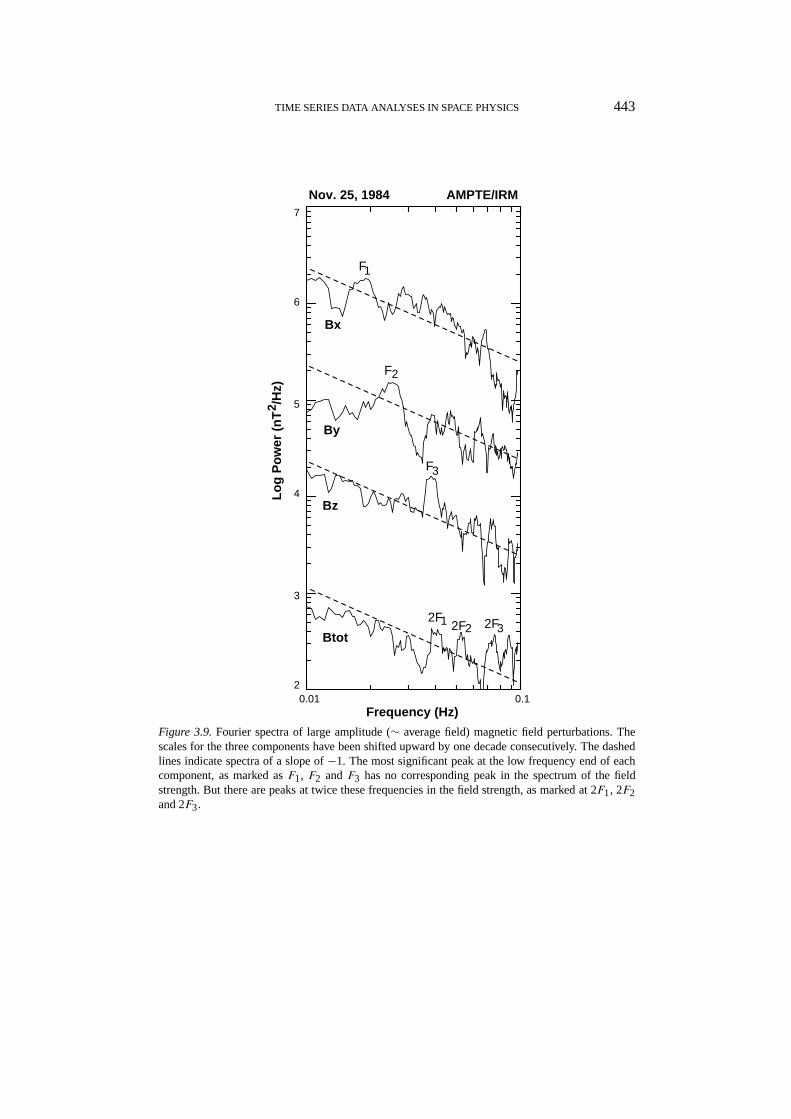
TIME SERIES DATA ANALYSES IN SPACE PHYSICS 443
Bx
By
Bz
Btot
Nov. 25, 1984 AMPTE/IRM
0.01 0.1
7
6
5
4
3
2
Frequency (Hz)
Lo
g P
ow
er (
nT
/H
z)2
F1
2
F3
2F1
F
2F 2F32
Figure 3.9.Fourier spectra of large amplitude (∼ average field) magnetic field perturbations. Thescales for the three components have been shifted upward by one decade consecutively. The dashedlines indicate spectra of a slope of−1. The most significant peak at the low frequency end of eachcomponent, as marked asF1, F2 andF3 has no corresponding peak in the spectrum of the fieldstrength. But there are peaks at twice these frequencies in the field strength, as marked at 2F1, 2F2and 2F3.

444 P. SONG AND C. T. RUSSELL
are usually measured by a search coil magnetometer in the same instrument pack-age. If all six components of the electric and magnetic fields are available, one isable to determine the Poynting flux of each wave. Analyzing plasma wave measure-ments largely relies on the dynamic spectral analysis as discussed in Sections 3.2.3and 3.2.9.
Here are some general guidelines to reading the spectra. If the enhancementsappear in both the electric and magnetic fields, the waves are eletromagnetic. Fromthe Faraday’s law, loosely speaking, the ratio between the power in the two com-ponents is the square of the phase velocity. For example, if the two spectra havea similar slope in a frequency range, the dispersion is weak in this range. If thestrength of the electric component increases faster with frequency than the mag-netic component, the phase velocity increases, and vice versa. If the enhancementsoccur only in the electric component, the waves are electrostatic. In this case, fromFaraday’s law, the wavevector is parallel to the electric perturbations and the phasevelocity cannot be derived by using the ratio between the electric and (zero) mag-netic amplitudes. Observationally, the latter may be largely determined by noise.Polarizations of the wave and the propagation direction (of electromagnetic waves)may be derived by examining the spin modulation of the signals (Scarf and Russell,1988; Strangeway, 1991; Song et al., 1998).
To interpret a plasma wave is generally more difficult than low frequency waves.The first difficulty one encounters is whether the wave is generated where it isobserved or not. Near the source region, a wave does not need to satisfy anyparticular dispersion because of the combination of the wave growth and possiblestrong spatial damping. One cannot assume a region of greater wave amplitude isthe source region because a greater amplitude does not necessarily mean a greaterwave energy flux. The phase velocity of a plasma wave is sensitive to the localplasma conditions. Strong waves usually occur in the region of rapid changes inplasma parameters. Many wave modes may be reflected at these boundaries whichcomplicates the possible interpretations. One has to examine carefully the plasmaparameters associated with the wave and estimate the unstable conditions for eachof the possible modes.
4. Spatial Correlation Analyses
Correlation analysis studies the relationship between measurements from differentobservation points. The observers can be either separated spacecraft in space ordifferent ground stations. When a disturbance or a wave travels from one observerto another, it is observed with a timing difference in the time domain or a phasedifference in the frequency domain between the two observers plus any change ofthe disturbance during the travel time period. From the timing or phase differenceand the separation between the two observers, one is able to determine the wavenumber of the wave. The change in the signal while propagating reduces the level
TIME SERIES DATA ANALYSES IN SPACE PHYSICS 445
of the correlation between the two observed signals and thus the time or phasedifference may be a function of frequency and possibly time.
4.1. BACKGROUND
4.1.1. Correlation Analysis in the Time DomainIf two observers measure the same quantity at different locations and the two timeseries data areQ(0, t) andQ(L , t), where we have assumed that the location ofthe first observer as the origin and the separation between the two observers isL ,the cross-correlation coefficient is defined as
α12(τ) = 1
K
t2∫t1
Q(0, t − 1/2τ)Q(L , t + 1/2τ) dt , (4.1)
wheret1 and t2 are the start and stop times of the selected interval, andK is thenormalization factor and is
K = t2−1/2τ∫t1−1/2τ
Q2(0, t) dt
t2+1/2τ∫t1+1/2τ
Q2(L , t) dt
1/2
.
The time lag with the highest cross-correlation coefficient can be used as the timingdifference,1t , between the two observers. The integration is realized through thesummation over the time window. In general, a narrower width of the windowprovides a greater maximum of the correlation coefficient because the noise withinthe window width may be likely weaker. For discontinuity analysis, one shouldselect a narrower window because for an ideal discontinuity, the cross-correlationcoefficient decreases as[1+ (|1t − τ |)/(t2 − t1)]−1. When the window is muchgreater than the time shift, the correlation coefficient appears flat. For wave analy-sis, a wider window, which includes several wave cycles will be statistically moresignificant.
If a wave is monochromatic, the correlation coefficient will periodically in-crease to unity and hence there is an ambiguity in determining the time lag. For-tunately, the waves in space are not purely monochromatic and one usually hasno difficulty to find a peak in the correlation coefficient with the greatest value.One still has to be careful since in some situations it is possible that the greatestcorrelation occurs associated with observations of different wave fronts.
What limits the resolution of the timing difference? If a wave is purely mono-chromatic, the resolution of the timing difference may be infinitely high, and de-pends on the accuracy of the clocks rather than the resolution of the data. However,because the waves in space are not monochromatic, as just discussed above, andalso because a wave may change slightly as it propagates from one observer toanother, or be slightly different at some distance along the wavefront where thesecond observation is made, there is uncertainty in the timing difference. This
446 P. SONG AND C. T. RUSSELL
uncertainty is anti-correlated with the value of the highest correlation coefficientand equal to or smaller than the resolution of the data. For example, since a dis-continuity departs most from an ideal monochromatic wave, the uncertainty in thetiming difference is the highest and equals half of the time resolution of the data.To minimize the uncertainty in timing discontinuities, one should use the data withthe highest resolution and filter the noise before an analysis. Otherwise, in commonpractice cross-correlation analysis is replaced by simply timing the delay of thediscontinuity between the two observers. When multiple waves are present, eachof them may have a different time delay. One needs to band-pass filter the databefore the correlation analysis. Otherwise, the time delay will be determined bythe wave of greatest power and the correlation coefficient will be smaller.
4.1.2. Correlation Analysis in the Frequency DomainIn the frequency domain, correlation analysis studies the phase difference betweenobservations at two locations. From this phase difference, one may be able todetermine the wave number.
If two time series data areQ(0, t) andQ(L , t) and their Fourier spectra areQ(0, ω) andQ(L , ω), the cross-correlation coefficient is
C12(ω) = 〈Q(0, ω)Q∗(L , ω)〉
K ′(ω), (4.2)
K ′ = [〈Q2(0, ω)〉〈Q2(L , ω)〉]1/2 ,where the asterisk stands for the conjugate and〈 〉 indicates an ensemble aver-age. The ensemble average is performed in time domain and equals the Fourierspectrum of the corresponding quantity in Equation (4.1) (e.g. Jenkins and Watts,1968). Note here that Equation (4.2) is different from that given in most theoreticalstudies. In theoretical studies, the ensemble average is performed over wavevector.While the wave vectors are obviously known in theory, observationally we believethat with a very limited number of observers we are still far from being able toresolve multiple wave modes at a single frequency.
Since the correlation coefficient in the frequency domain is complex, it can bewritten as
C12(ω) = κ2(ω)eiφ(ω) , (4.3)
whereκ(ω) andφ(ω) are coherence and phase lag, respectively. The coherencegives a measure of wave versus noise. The noise can be either due to randomfluctuations or due to waves with a finite coherence length compared with theseparation between the two observers. The coherence length along a wavefrontis the spatial scale of the wave. The coherence length normal to the wavefront isroughly the traveling distance of the wave, including both convection and propa-gation, within its decay time. For example, since the convection speed of the solarwind is much greater than the phase velocity, the waves in the solar wind often have

TIME SERIES DATA ANALYSES IN SPACE PHYSICS 447
larger coherence length along the flow than transverse to the flow. The differencebetween random fluctuations and waves with a coherence length shorter than theseparation is that the power spectra are broad for the former and at least one ofthem is peaked for the latter.
If the noise is due to random fluctuations, the phase difference of a wave be-tween two observers is
φ(ω) = k · L + h2π , (4.4)
whereh = 0,±1, . . . . Thus, the wave number can be determined, but with the so-called 2π ambiguity. Here the direction of the wave vector is determined from themethods discussed in Sections 3.1 and 3.2. Since the frequency in Equation (4.4)is in the spacecraft frame, further determination of the wave properties needs toconsider the Doppler shift, Equation (3.18). The time lag can be calculated from1t = φ(ω)/ω, which is a function of frequency.
In summary, correlation analysis can determine either the propagation speed ofa discontinuity or the wavelength of a wave. For a discontinuity, the correlationanalysis has to be performed in the time domain. For a wave, the analysis canbe performed in either the time domain or the frequency domain. The analysisin the frequency domain contains the information about the phase as functions offrequency and hence can provide a better overall view of the waves at differentfrequencies. The result of an analysis in the frequency domain is in principle thesame as in the time domain with prefiltering. These analyses are restricted to wavesof a single source.
4.1.3. Relationship between the Quantities in Satellite Frame and Plasma FrameIn Section 1.1, we discussed the relationship between a quantity in the satelliteframe and in the plasma frame for a single spacecraft. When comparing observa-tions from two satellites at different times, the variations other than simple convec-tion from one satellite to the other will affect the data analysis. These variationsinclude spatial (between the two satellites) and temporal (between the two times)variations due to the physical evolution of the phenomenon being studied, andchanges in the velocity and spacecraft separation.
The difference between the quantityQ measured by satellitei at locationr attime t and by satellitej separated by a distanceL ij from satellitei at timet + τ is,see Figure 4.1 for the geometry,
1ijτ Q = Qj(r + L ij − vτ, t + τ)−Qi(r , t) , (4.5)
whereτv should be understood as∫
v dt. A time domain correlation analysis isto provide time shift1t = τ with a minimal difference, i.e.,1ij
τ Q goes to zero.Taylor expanding Equation (4.5) and retaining the terms up to the second order, thedifference operator is

448 P. SONG AND C. T. RUSSELL
A(x,t)
A'(x - vτ, t+τ)
B(x+L,t)B'(x+L- vτ, t+τ)
vτ
Figure 4.1.Geometry of two separated spacecraft relative to a wave front. Satellite A is located atpoint A and satellite B at point B. The plasma element that is measured by satellite A at timet andthe plasma element at point A′ is measured att + τ . Similarly, the plasma element that is measuredby satellite B att + τ is from point B′. A correlation analysis compares measurements at differentlocations and/or different times.
1ijτ =
[(τ∂
∂t− τv · ∇
)+ L ij · ∇
]+
+[τ
2
(τ∂
∂t− τv · ∇ + L ij · ∇
)∂
∂t
]−
−[τ
2
(τ∂
∂t− τv · ∇ + L ij · ∇
)(v · ∇)
]+
+[
1
2
(τ∂
∂t− τv · ∇ + L ij · ∇
)(L ij · ∇)
].
(4.6)
We should point out that the validity of the Taylor expansion relies onL ij − vτ tobe much smaller thanLc andτ to be much smaller thantc, whereLc andtc are thecoherence length and coherence time, respectively. Whereas the measured quantitycan contain discontinuities. Namely,L ij is not necessarily much smaller than thescale of the discontinuities (in the normal direction). As long as the correlationanalysis provides a meaningful correlation, the Taylor expansion is valid. The termsin the first bracket are due to the linear effects. The main differences observed bythe two spacecraft are caused by the temporal variations in the plasma frame and

TIME SERIES DATA ANALYSES IN SPACE PHYSICS 449
the spatial non-uniformity of the plasma along the motion direction and along theseparation direction of the two spacecraft. The function of the correlation analysisis to provide aτ that minimizes the value in this bracket. Namely, the correla-tion analysis converts linearly the temporal variations in the spacecraft frame intospatial variations in the plasma frame of reference. It is less capable of providinginformation about spatially static structures in the spacecraft frame. In general thenonlinearities in the temporal and spatial variations will result in a residue for theseterms. This residue reduces the correlation coefficient of the analysis. The terms inthe second bracket are due to the nonlinear effects of temporal variations. The termsin the third bracket are due to the nonlinear effects of nonsteady state, nonuniformplasma motion. Similarly, the terms in the fourth bracket are due to the temporaland spatial changes in the separation between the two spacecraft.
In most cases, the variations in the separation vector (the fourth bracket) arenegligibly small. The velocity variation (the third bracket) could become signif-icant near an oscillating boundary and for a circularly polarized wave the veloc-ity of which could be twisted by the wave perturbations, in particular when thebackground velocity is small.
For a single spacecraft,L = 0, the first order terms recovers Equation (1.1).Note that the velocity in Equation (4.6) is not necessarily the plasma velocity butcould be the velocity of any frame relative to the spacecraft. In a shock frame ora wave frame,∂/∂t = 0. The first order term is(L ij − vτ) · ∇. In the ideal 1-Dcase,1ij
τ = 0 whereτ is defined as the time delay with the maximum correlationcoefficient, and it yields equations (2.20) and (3.20) by noting that the speed ofthe wave frame relative to the spacecraft is the sum of the phase velocity and theplasma frame speed.
4.1.4. Data Analysis of Observations from a Cluster of SatellitesA ‘cluster’ of spacecraft refers to four closely separated satellites. The relativelocations of the satellites can be represented in general by an irregular tetrahedron.Regulated by orbital dynamics, the shape of the tetrahedron changes with time. Ifthe change in their relative distance is much less than in the relative distance itselfduring the interval of the event being studied, the change of the tetrahedron maybe neglected. The uncertainties in the determination of the relative locations andin the intracalibration of the instruments among the satellites determine the lowerlimit of the uncertainty of any analysis.
In principle, when the cluster is not coplanar, the propagation direction of a 1-Ddiscontinuity or a 1-D steady state wave can be determined without the assump-tion that the propagation direction is along the minimum variance direction. Withthe approximation that the propagation direction is along the minimum variancedirection, either the unsteadiness of the wave (in the wave frame), or a 2-D steadystate structure or wave can be resolved under certain conditions. A moving fluxtube with a constant shape is an example of a 2-D steady state structure. A purelyperiodic surface wave in the wave frame is an example of the 2-D steady state

450 P. SONG AND C. T. RUSSELL
wave. For a given perturbation, even with a noncoplanar cluster of satellites, thereis no general conclusive interpretation. One has to make approximations about eachof the extension in three dimensions (bounded, periodic, or uniform) and its timedependence (pulsating, periodic, or steady). Differences in these approximationslead to different interpretations, which has been the major cause of existing contro-versies in the science community. Each of these approximations, however, can betested both using either the information from other instruments or techniques thatare not included in this article as standard techniques, and using the constraintsprovided by statistics and physical consequencies.
In the following sections, we discuss the application of correlation analysis tomultiple spacecraft observations. Most discussion is based on the authors’ expe-rience from previous missions and recent results from other groups. We empha-size that the problems with massive multiple spacecraft data analysis have not yetbeen fully exposed. Significant modification may be needed when applying thefollowing principles.
4.2. ONE-DIMENSIONAL DISCONTINUITY ANALYSES
As discussed in Section 2.1.1, to completely determine observationally the prop-erties of a 1-D steady state discontinuity, more than one satellite is needed. Thecentral issue is to determine the direction and magnitude of the velocity of theshock frame relative to the spacecraft without imposing the conservation lawswhich should be verified by the results. The timing difference between spacecrafti andj is
1tij = L ij · Vdisc/V2disc . (4.7)
Note that, as discussed at the end of Section 4.1.3, the above expression isaccurate to the first order and only for an ideal steady-state 1-D discontinuity. Incomparison, Equation (1.2) does not require the steadiness approximation. Withfour spacecraft,Vdisc can be uniquely determined if the four spacecraft are notcoplanar. With five noncoplanar spacecraft, Equation (4.7) can become overdeter-mined andVdisc can be determined using best-fit, for example, or average over theseveralVdisc obtained from each subset of the four time differences (Russell et al.,1983). In practice, one may obtain several time delays crossing a discontinuity foreach pair of spacecraft, for example, one at the leading edge, one in the middleand one at the trailing edge, when using high resolution data. If one assumes thatthe difference between the two time delays is not due to temporal variation ofthe thickness, averaging these sets will improve the statistical significance of theresults.
Using the resultantVdisc and Equation (2.7), one can derive the quantities inthe R–H relations. The accuracy of the time delay is limited by the temporalresolution of the data when the fluctuations within the discontinuity cannot beresolved. A greater time delay compared with the temporal resolution implies a

TIME SERIES DATA ANALYSES IN SPACE PHYSICS 451
Figure 4.2. As a surface wave passes by two spacecraft, a few timing differences and normaldirections can be obtained in order to determine the parameters of the surface wave.
smaller uncertainty in the timing, whereas during this longer interval, there is agreater chance for the discontinuity to change its properties. If the resolution issufficiently high, the thickness of the discontinuity then can be determined fromthe duration of the crossing. If the spacraft are relatively close, a major uncertaintyarises from the determination of the relative locations of the spacecraft.
If the type of the discontinuity is known or the techniques discussed in Section 2are applicable, a combination of the timing method with those in Section 2 willimprove the statistical significance of the results. In addition, one may be able tofind intervals when the discontinuity lies between the spacecraft and hence someof them provide the upstream conditions while others the downstream ones. Quan-tities in Equations (2.10) and (2.11) can be substituted with those simultaneouslymeasured by different satellites instead of those measured at different times fromthe same satellite.
Since each method has its own uncertainty, when averaging results from dif-ferent methods, how to weigh each of them becomes important. Russell et al.(1983) documented several cases and provided comprehensive discussions on theuncertainties.
Nonsteadiness of a discontinuity is observed as the difference in the durationof the discontinuity crossing registered among different satellites and the differ-ence in the time shifts. It can be treated as the variation around the average. Thenonsteadiness includes the temporal variations in the discontinuity’s orientation(i.e., its normal direction) and the thickness, and the changes in the shock velocityrelative to the satellites.
4.3. TWO DIMENSIONAL STRUCTURES
4.3.1. Surface Wave AnalysesSurface waves in magnetospheric physics refer to the wavy motion of a discontinu-ity. To describe such a motion, the most important parameters are the wavelengthand the displacement, as well as the period. The wavelength is measured alongthe discontinuity surface in the direction of the surface wave propagation and thedisplacement is normal to the average surface. Simple boundary oscillations are a1-D approximation when the wavelength is infinity. With a finite wavelength, thediscontinuity is bent. As expected, the boundary normal varies. If the thickness of

452 P. SONG AND C. T. RUSSELL
the boundary is much smaller than the curvature of the boundary the discontinuityanalysis methods discussed in Section 2 are applicable. The normal direction of theboundary can be determined by each of the crossings. The variation in the normaldirection can then be measured by the satellites, see Figure 4.2 for example. Withmultiple satellites, one is able to determine the characteristics of a surface wave(Song et al., 1989). Mottez and Chanteur (1994) discussed a similar technique toanalyze a general 3-D thin surface using a cluster of satellites.
A different approach has been recently developed using the ‘remote sensing’technique (Walthour et al., 1993). As a boundary oscillates, the plasma and fieldparameters in the regions adjacent to the boundary vary. For example, the math-ematical description of a surface wave is an exponential decay in the amplitudeof the perturbation away from the boundary (e.g., Southwood, 1968). From thesevariations, a satellite can remotely sense the boundary and its motion when itapproaches to and departs from the boundary. This new technique requires highquality measurements. It has been tested by using two-satellite data (Walthouret al., 1994).
4.3.2. Flux TubeWhen the plasma beta is not extremely large, the anisotropy in a plasma introducedby the field often results in structures that have similar sizes in the two directionsacross the field and their greatest scale size along the field. Usually such a structurehas properties distinct from its surrounding plasmas. Russell et al. (1990) provideda collection of comprehensive discussions on flux tubes from various regions inspace. The majority of previous observations are based on single spacecraft mea-surements. The geometry of a structure, for example, a flux transfer event (Russelland Elphic, 1978) or a plasmoid, is often deduced from time series data (which pro-vides the variation in one dimension), the region where it is observed on a statisticalbasis (which provides the scale of the second dimension), and the assumption thatthe structure is very long in the third dimension. Sometimes, observations frommultiple satellites are available. Examination of these events confirms the generalgeometry people have developed for these phenomena.
A cluster of spacecraft can provide much more detailed information about theseflux tubes. A general approach to analyzing these structures is similar to that ofsurface waves.
It is worth mentioning that since a flux tube does not satisfy the 1-D approxi-mation, the minimum variance direction across the event may not have any definitemeaning. For example, unless there are other indications, one should not take themininum variance direction as the direction of the symmetric axis because theaxial field may increase toward the axis due to a pinch process that arises froman axis-aligned current within the tube.

TIME SERIES DATA ANALYSES IN SPACE PHYSICS 453
4.4. DETERMINATION OF ELECTRIC CURRENTS
The electric current is a very important physical quantity in space physics. How-ever it is extremely difficult to measure in space. Because the conductivity in acollisionless plasma is poorly known, Ohm’s law cannot be used to evaluate thecurrent. In theory, there are two ways to measure the current. They are
J =∑i
qiρivi , (4.8)
J = 1
µ0∇ × B , (4.9)
where subscripti denotes each charge species. As discussed in Section 1.3.3, itis difficult to measure accurately the fluxes of the species that carry most of thecurrent due to the intrinsic limitation of particle detectors and spacecraft charging.This is particularly true in collisionless plasmas where particle gyro motions aredominant. In most regions in the magnetosphere, the relative drift between ionsand electrons is small. The limitation of instruments further reduces the abilityof resolving such a small difference. For example, as shown in Equation (1.10),the effective cutoff velocity of a detector depends on the species. The spacecraftcharge will have much greater effects on electron detection than on ion detection.When the spacecraft is strongly negatively charged, the difference in the errors inthe velocity measurements will produce a large error in evaluating Equation (4.8)even if the detector has a similar small lower cutoff energies for electrons and ions.Although there are several reports on the determination of the electric current usingEquation (4.8), see Frank et al. (1981), for a partially successful test, we remaincautious about quantitative use of the current from direct particle measurements.
4.4.1. Single SatelliteEquation (4.9) has been widely used to estimate the current. Almost all previoussingle satellite usage was based on a 1-D current sheet assumption. In 1-D
Jm = 1
µ01Bl/D ,
Jl = − 1
µ01Bm/D , (4.10)
whereD is the thickness of the current sheet across which1B is evaluated. TodetermineD from a time difference, one needs to know the velocity of the currentlayer relative to the spacecraft. Therefore all discussions given in Section 2 ondetermination of the shock frame apply here.
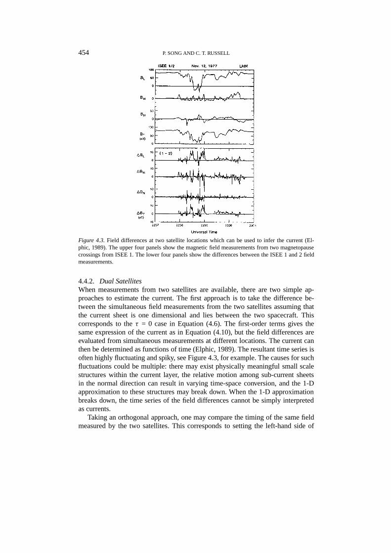
454 P. SONG AND C. T. RUSSELL
Figure 4.3.Field differences at two satellite locations which can be used to infer the current (El-phic, 1989). The upper four panels show the magnetic field measurements from two magnetopausecrossings from ISEE 1. The lower four panels show the differences between the ISEE 1 and 2 fieldmeasurements.
4.4.2. Dual SatellitesWhen measurements from two satellites are available, there are two simple ap-proaches to estimate the current. The first approach is to take the difference be-tween the simultaneous field measurements from the two satellites assuming thatthe current sheet is one dimensional and lies between the two spacecraft. Thiscorresponds to theτ = 0 case in Equation (4.6). The first-order terms gives thesame expression of the current as in Equation (4.10), but the field differences areevaluated from simultaneous measurements at different locations. The current canthen be determined as functions of time (Elphic, 1989). The resultant time series isoften highly fluctuating and spiky, see Figure 4.3, for example. The causes for suchfluctuations could be multiple: there may exist physically meaningful small scalestructures within the current layer, the relative motion among sub-current sheetsin the normal direction can result in varying time-space conversion, and the 1-Dapproximation to these structures may break down. When the 1-D approximationbreaks down, the time series of the field differences cannot be simply interpretedas currents.
Taking an orthogonal approach, one may compare the timing of the same fieldmeasured by the two satellites. This corresponds to setting the left-hand side of

TIME SERIES DATA ANALYSES IN SPACE PHYSICS 455
Equation (4.6) zero. Under the assumption that the structure of the current is sta-tionary, but the motion of the current changes with time, retaining the first orderterms, the velocity of the current layer can then be calculated by dividing the satel-lite separation along the normal of the current by the timing difference between thetwo satellites’ measuring of the same magnetic field, as shown by Equation (4.7).When the velocity of the current layer is known, from Equation (4.10) one candetermine the current according to the time series of each satellite, see Figure 4.4.In theory, the currents derived from the two satellites should be the same if thecurrent is in steady state. In fact, the resultant currents are different, indicating thatthe current is not in a steady state. How to reconcile this inconsistency remains tobe investigated.
Often the two spacecraft are on the same side of the current sheet (after passingthrough or before the crossing) at different times. These data on the same sidecan be used to help test the 1-D time stationary assumption by combining the twoapproaches above.
4.4.3. Multiple SatellitesThe above techniques rely on the 1-D assumption of the current. The measurementsfrom a cluster of satellites will enable us to determine the spatial derivatives andhence the current in Equation (4.9) without the 1-D assumption. The spatial deriv-ative method applied to a quasi-stationary current system is very different from theanalysis of a fast moving current structure. In the former case, correlation analysismay not be able to provide a meaningful timing difference. Therefore the approachof settingτ equal to zero is used. In the latter case,τ can be determined and hencemore information is available to measure the current and its motion velocity.
4.4.3.1. Quasi-stationary currents. A current system can be considered as quasi-stationary if|1ijB| � |1τB|Lij /τV , where V is the velocity of the current systemrelative to the spacecraft (note here that whenV = 0, τ goes to infinity). Inother words, the measured temporal variation in the field is much smaller thanthe difference among satellites. This assumption is applicable for a cluster movingslowly through a current region that is thicker than the separation of the satellites.The electric current density can be determined by (Dunlop et al., 1988),
Jijk = 1
µ0
1ijB · L jk −1jkB · L ij(L ij × L jk)2
. (4.11)
The direction ofJijk is outward along the normal direction of the surface formedby spacecraft i, j, and k. Four suchJijk can be obtained. The current density withinthe cluster can be calculated by averaging the four current densities. The directionof the current,J is parallel to the vector summation ofJijks, and its magnitude is
J = (Jijk|L ij × L jk|)J · (L ij × L jk)
. (4.12)

456 P. SONG AND C. T. RUSSELL
Figure 4.4.Two-satellite determination of the current (McComas et al., 1986). Under the 1-D steadystate assumption of the current structure, the velocity of the current motion can be determined, middlepanel, and then the current density can be derived, lower panel.
An important test of the result is to check whether the sum ofJijk · (L ij × L jk) ismuch smaller than each of them.
We should emphsize that the approach under the steady state approximation isnot the same as the approach when the spacecraft separations are much smallerthan the spatial scale of the current structure. When two spacecraft see basicallydifferent things, the correlation analysis does not provide anything meaningful.
4.4.3.2. Traveling current structures. Current systems in space often move quicklyrelative to the satellites. A boundary or surface, that is neither necessarily thinnerthan the spacecraft separation nor planar, can pass a cluster of spacecraft quickly

TIME SERIES DATA ANALYSES IN SPACE PHYSICS 457
without significant changes in itself. Under this circumstance, the correlation analy-sis can provide very important information. Note here that more than one time shift(here one may use the measured timing difference directly instead of performing acorrelation analysis because to perform the correlation analysis at each of the edgesis usually very difficult) can be determined for a single passage of the current foreach pair of spacecraft, at its leading and trailing edges. Averaging the velocitiesobtained from Equation (4.7) for all satellite pairs, one yields the velocity of thecurrent structure. Here we recall that there is no assumption made on the shapeor normal of the structure when using Equation (4.7) and hence it is applicableto structures of any regular shape. The geometry of the current structure can beexamined according to the timing difference of each pair from the average andtheir relative locations.
With the derived velocityV0, the current density at spacecrafti can be calcu-lated by
Ji = 1
µ0∇ × Bi = 1
µ0V0−1× δBi
δti, (4.13)
where prefixδ denotes the difference measured from the same spacecraft at differ-ent times, andV−1
0 = (1/Vx, 1/Vy, 1/Vz). Although this expression is meaningfulin theory, in practice the fluctuations in the smallest component of the velocity andthe magnetic fluctuations perpendicular to the smallest velocity component maycause a very large uncertainty in the calculation. One should keep caution in usingit.
4.5. WAVE ANALYSES
In wave analysis, the time derivatives in Equation (4.6) are, in general, not zero inthe spacecraft frame. The approach that setsτ = 0 will eliminate all the terms offrequency and hence cannot be used to analyze waves. With a non-coplanar clusterof four spacecraft, in principle, one is able to determine the frequency, wavelengthand phase velocity of a planar wave if its wavelength is of the order of spacecraftseparation. For waves with a wavelength that is either much greater or smaller thanthe spacecraft separation, there is no general method to derive all these three waveparameters.
For perturbations that can be approximated as 1-D, but not necessarily mono-chromatic, one can follow the general steps.
(1) Select the perturbations of interest and band-pass filter the time series data.Note that if the wave is not monochromatic, the spectrum will have finite width.
(2) Perform wave analysis to determine the direction of the wave propagationfor each spacecraft, and take the average of these vectors as the direction of thewave vector.
(3) Perform correlation analysis for each component of the filtered data usingeach pair of spacecraft.

458 P. SONG AND C. T. RUSSELL
Figure 4.5.Many wave modes pass across a cluster of satellites (Neubauer and Glassmeier, 1990).
(4) Calculate the apparent velocity of the perturbation from the correlationanalysis and compare its direction with the direction of the wave derived fromthe wave analysis.
(5) Analyze the deviation of each quantity from its corresponding average. Ingeneral, these deviations can be attributed to temporal variations that may not bedirectly related to the wave.
The biggest difficulty one may face here is that there is too much informationand some of these pieces are in conflict. While one could use average and nor-malization to enhance the robustness of the results, we suggest one leave enoughroom for different possible interpretations because we think that at this momentwe have very limited knowledge about the problems inherent in an analysis ofsuch complexity.
Neubauer and Glassmeier (1990) proposed the concept of wave-telescope. Asillustrated in Figure 4.5, when a wave propagates across a cluster of satellites, eachsatellite observes a different phase according to the wave propagation direction andthe relative location among them. From these phase shifts, in theory, one is able toderive the wave properties. There are established techniques in radio science toanalyze such information. While this proposal is intriguing, we note that in spacewave analysis the signal-noise ratio is often low. Multiple modes in space plasmaoften exist, see Section 3.3 for more details, and are difficult to distinguish. Oftenwhen testing with a known wave, a scheme may work, but there may be multiplesolutions when the input is unknown.

TIME SERIES DATA ANALYSES IN SPACE PHYSICS 459
5. Discussion and Summary
Although it seems mathematically trivial, Equation (1.2) is one of the most impor-tant results in our review. It describes all physical effects on the measured magneticfield and provides a rigorous theoretical foundation for minimum variance analysesof the magnetic field. It shows that the minimum variance analyses are based ona one-dimensional assumption but do not require a steady state. If the minimumvariance analyses also depended on the steady state assumption as many peoplepercieved since it was first developed to analyze discontinuity, it would not havebeen applicable to wave analysis.
Another fundamental result is the derivation of Equation (4.6) which providesa unified theory for correlation analyses. Every existing correlation analysis tech-nique can be found to be a special case of this equation. This expression specifiesclearly the assumptions upon which each technique is based. In developing dataanalysis methods for Cluster missions, one needs to compare the methods againstthis expresion in order to identify the effects that are neglected in the methods andjustify for the simplification. We emphasize that at the practical level there has notyet been sufficient analysis of multiple satellites data to test and refine many of thetechniques discussed herein.
On one hand, discontinuity analysis is, among time series data analysis meth-ods, best understood and its computer programs are most user-friendly. It is widelyused. However, on the other hand, the errors of the analysis have not been recog-nized as widely as it should. Ocasionally, one may see in publication a discontinuityis presented in boundary normal coordinates with an unequal normal magnetic fieldacross it.
Multiple parameter best fits are often used to determine unmeasured shockparameters. As we now know that this method in practice usually has a largeuncertainty and may provide a large range of solutions with a small differencein input parameters. Here we again urge caution in using this method.
In wave analysis, a common trend is that fewer and fewer people actually ana-lyze the time series data itself, and more and more people rely on dynamic spec-trograms. Ocasionally, one sees that a field rotation is interpreted as broadbandemission that last for a period of the window length. Here we strongly urge analyststo examine the original time series data. On the other hand, there is a significantroom for further improving the techniques of wave analysis.
In addition to mastering the various analysis methods, an analyst has to possessadequate knowledge of the data set he/she is using. From our experience, directcollaboration with an builder of the instrument is an effective way to ensure thatthe data is utilized correctly. However this is still no substitute for the properdocumentation of the instruments and the data stream.

460 P. SONG AND C. T. RUSSELL
Acknowledgments
This work was supported by NASA under research grants NAGW–3948, NAGW–3974, NAG5–4066 and NAG5–3880 to UCLA, and by National Science Foun-dation/Office of Naval Research under research grant NSF–ATM 9713492. Theauthors are grateful to Bengt Sonnerup for useful discussions.
References
Anderson, T. W.: 1978,An Introduction to Multivariate Statistical Analysis, John Wiley and Sons,New York.
Anderson, B. J., Fuselier, S. A. and Murr, D.: 1991, ‘Electromagnetic Ion Cyclotron Waves Observedin the Plasma Depletion Layer’,Geophys. Res. Letters.18, 1955.
Arthur, C. W., McPherron, R. L. and Means, J. D.: 1976, ‘A Comparative Study of Three Techniquesfor Using the Spectral Matrix in Wave Analysis’,Radio Sci.11, 833.
Barnes, A. and Hollweg, J. V.: 1974, ‘Large-Amplitude Hydromagnetic Waves’,J. Geophys. Res.79,2302.
Born, M. and Wolf, E.: 1965,Principles of Optics, Pergamon Press Inc., Oxford.Chao, J. K.: 1970,Interplanetary Collisionless Shock Waves, Rep. CSR TR-70-3, Mass. Inst. of
Technology, Center for Space Res., Cambridge, Mass.Chao, J. K.: 1995, ‘Intermediate Shocks: Observations’,Adv. Space Res.15 (8/9), 521.Chao, J. K., Zhang, X. X. and Song, P.: 1995, ‘Derivation of Temperature Anisotropy from Shock
Jump Relations: Theory and Observations’,Geophys. Res. Letters22, 2409.Colburn, D. S. and Sonett, C. P.: 1966, ‘Discontinuities in the Solar Wind’,Space Sci. Rev.5, 439.Crooker, N. U. and Siscoe, G. L.: 1979, ‘A Mechanism for Pressure Anisotropy and Mirror Instability
in the Dayside Magnetosheath’,J. Geophys. Res.82, 185.Denton, R. E., Gary, S. P., Lin, X., Anderson, B. J, LaBelle, J. W. and Lessard, M.: 1995, ‘Low-
Frequency Fluctuations in the Magnetosheath Near the Magnetopause’,J. Geophys. Res.100,5665.
Dunlop, M. W., Southwood, D. J., Glassmeier, K.-H. and Neubauer, F. M.: 1988, ‘Analysis ofMultipoint Magnetometer Data’,Adv. Space Res.8, (9), 273.
Elphic, R. C.: 1989, ‘Multipoint Observations of the Magnetopause: Results from ISEE andAMPTE’, Adv. Space Res.8, (9), 223.
Frank, L. A., McPherron, R. L., DeCoster, R. J., Burek, B. G., Ackerson, K. L. and Russell, C. T.:1981, ‘Field-Aligned Currents in the Earth’s Magnetotail’,J. Geophys. Res.86, 687.
Gary, S. P.: 1992, ‘The Mirror and Ion Cyclotron Anisotropy Instabilities’,J. Geophys. Res.97, 8519.Gary, S. P. and Winske, D.: 1992, ‘Correlation Function Ratios and the Identification of Space Plasma
Instabilities’,J. Geophys. Res.97, 3013.Harvey, C. C., Etcheto, J., De Javel, Y., Manning, R. and Petit, M.: 1978, ‘The ISEE Electron Density
Experiment’,IEEE Trans. Geosci. Electron.GE-16, 231.Hoppe, M. M., Russell, C. T., Frank, L. A., Eastman, T. E. and Greenstadt, E. W.: 1981, ‘Upstream
Hydromagnetic Waves and Their Association with Backstreaming Ion Populations: ISEE 1 and3 Observations’,J. Geophys. Res.86, 4471.
Jenkins, G. M. and Watts, D. G.: 1968,Spectral Analysis and Its Applications, Holden-Day, London,p. 525.
Kantrowitz, A. and Petschek, H. E.: 1966, in W. B. Kunkel (ed.), ‘MHD Characteristics and ShockWaves’,Plasma Physics in Theory and Application, McGraw-Hill Book Co., New York, p. 494.
Kawano, H. and Higuchi, T.: 1995, ‘The Bootstrap Method in Space Physics: Error Estimation forthe Minimum Variance Analysis’,Geophys. Res. Letters22, 307.

TIME SERIES DATA ANALYSES IN SPACE PHYSICS 461
Kepko, E., Khurana, K. K. and Kivelson, M. G.: 1966, ‘Accurate Determination of Magnetic FieldGradients from Four Point Vector Measurements: 1. Use of Natural Constraints on Vector DataObtained from Single Spinning Spacecraft’,IEEE Trans. Geosci. Electron.32, 377.
Khurana, K. K., Kepko, E., Kivelson, M. G. and Elphic, R. C.: 1996, ‘Accurate Determination ofMagnetic Field Gradients from Four Point Vector Measurements: 2. Use of Natural Constraintson Vector Data Obtained from Four Spinning Spacecraft’,IEEE Trans. Geosci. Electron.32,5193.
Kivelson, M. G. and Russell, C. T.: 1995,Introduction to Space Physics, Cambridge University Press,p. 567.
Kodera, K., Gendrin, R. and De Villedary, C.: 1977, ‘Complex Representation of a Polarized Signaland Its Application to the Analysis of ULF Waves’,J. Geophys. Res.82, 1245.
Krauss-Varban, D. and Omidi, N.: 1993, ‘Propagation Characteristics of Wave Upstream andDownstream of Quasi-Parallel Shocks’,Geophys. Res. Letters.20, 1007.
Krauss-Varban, D., Omidi, N. and Quest, K. B.: 1994, ‘Mode Properties of Low-Frequency Waves:Kinetic Theory versus Hall-MHD’,J. Geophys. Res.99, 5987.
LaBelle, J. and Treumann, R. A.: 1988, ‘Plasma Waves at the Dayside Magnetopause’,Space Sci.Rev.47, 175.
Le, G., Russell, C. T. and Smith, E. J.: 1989, ‘Discrete Wave Packets Upstream from the Earth andComets’,J. Geophys. Res.94, 3755.
Lee, L. C., Price, C. P. and C. S. Wu: 1988, ‘A Study of Mirror Waves Generated Downstream of aQuasi-Perpendicular Shock’,J. Geophys. Res.93, 274.
Lepidi, S., Villante, U., Lazarus, A. J., Szabo, A. and Paularena, K.: 1996, ‘Observations of BowShock Motion During Times of Variable Solar Wind Conditions’,J. Geophys. Res.101, 11107.
Lepping, R. P. and Behannon, K. W.:1980, ‘Magnetic Field Directional Discontinuities: 1. MinimumVariance Errors’,J. Geophys. Res.85, 4695.
Lin, Y. and Lee, L. C.: 1994, ‘Structure of Reconnection Layers in the Magnetosphere’,Space Sci.Rev.65, 59.
McComas, D. J., Russell, C. T., Elphic, R. C. and Bame, S. J.: 1986, ‘The Near-Earth Cross-TailCurrent Sheet: Detailed ISEE 1 and 2 Case Studies’,J. Geophys. Res.91, 4287.
McPherron, R. L., Russell, C. T. and Coleman, P. J., Jr.: 1972, ‘Fluctuating Magnetic Fields in theMagnetosphere: II ULF Waves’,Space Sci. Rev.13, 411.
Means, J. D.: 1972, ‘Use the Three-Dimensional Covariance Matrix in Analyzing the PolarizationProperties of Plane Waves’,J. Geophys. Res.77, 5551.
Mellott, M. M. and Greenstadt, E. W.: 1984, ‘The Structure of the Oblique Subcritical Bow Shock:ISEE 1 and 2 Observations’,J. Geophys. Res.89, 2151.
Mottez, F. and Chanteur, G.: 1994, ‘Surface Crossing by a Group of Satellites: A Theoretical Study’,J. Geophys. Res.99, 13499.
Mozer, F. S., Hones, E. W., Jr. and Birn, J.: 1983, ‘Comparison of Spherical Double Probe ElectricField Measurements with Plasma Bulk Flows in Plasmas Having Densities Less than 1 cm−3’,Geophys. Res. Letters10, 737.
Mozer, F. S., Cattell, C. A., Temerin, M., Torbert, R. B., Von Glinski, S., Woldorff, M. and Wygant,J.: 1979, ‘The dc and ac Electric Field, Plasma Density, Plasma Temperature, and Field-AlignedCurrent Experiments on the S3-3 Satellite’,J. Geophys. Res.84, 5875.
Neubauer, F. M. and Glassmeier, K.-H.: 1990, ‘Use of an Array of Satellites as a Wave Telescope’,J. Geophys. Res.95, 19115.
Newbury, J. A., Russell, C. T. and Gedalin, M.: 1997, ‘The Determination of Shock Ramp Thicknessusing the Noncoplanar Magnetic Field Component’,Geophy. Res. Letters24, 1975.
Omidi, N. and Winske, D.: 1995, ‘Structure of the Magnetopause Inferred from the Kinetic RiemannProblem’,J. Geophys. Res.100, 11935.
Petrinec, S. M. and Russell, C. T.: 1993, ‘Intercalibration of Solar Wind Instruments During theInternational Magnetospheric Study’,J. Geophys. Res.98, 18963.

462 P. SONG AND C. T. RUSSELL
Rankin, D. and Kurtz, R.: 1970, ‘Statistical Study of Micropulsation Polarizations’,J. Geophys. Res.75, 5445.
Russell, C. T.: 1988, BANAL: A Computer Program for the Display and Analysis of MagnetometerData, April 1988.
Russell, C. T.: 1983, ‘Interactive Analysis of Magnetic Field Data’,Adv. Space Res.2 (7), 173.Russell, C. T. and Elphic, R. C.: 1978, ‘Initial ISEE Magnetometer Results: Magnetopause
Observations’,Space Sci. Rev.22, 681.Russell, C. T., Childers, D. D. and Coleman, P. J., Jr.: 1971, ‘OGO-5 Observations of Upstream
Waves in the Interplanetary Medium: Discrete Wave Packets’,J. Geophys. Res.76, 845.Russell, C. T., Mellott, M. M., Smith, E. J. and King, J. H.: 1983, ‘Multiple Spacecraft Observations
of Interplanetary Shocks: Four Spacecraft Determination of Shock Normals’,J. Geophys. Res.88, 4739.
Russell, C. T., Riedler, W., Schwingenschuh, K. and Yeroshenko, Y.:1987, ‘Mirror Instability in theMagnetosphere of Comet Halley’,Geophys. Res. Letters14, 644.
Russell, C. T., Priest, E. R. and Lee, L. C.: 1990,Physics of Magnetic Flux Ropes, GeophysicalMonograph, Vol. 58, AGU, Washington.
Scarf, F. L. and Russell, C. T.: 1988, ‘Evidence of Lightning and Volcanic Activity on Venus’,Science240, 222.
Sckopke, N., Paschmann, G., Brinca, A. L., Carlson, C. W. and Luhr, H.: 1990, ‘Ion Termalizationin Quasi-Perpendicular Shocks Involving Reflected Ions’,J. Geophys. Res.95, 6337.
Song, P., Elphic, R. C., Russell, C. T.: 1989, ‘Multi-Spacecraft Observations of Magnetopause Sur-face Waves: ISEE 1 and 2 Determinations of Amplitude, Wavelength and Period’,Adv. SpaceRes.8, (9), 245.
Song, P., Russell, C. T. and Thomsen, M. F.: 1992, ‘Waves in the Inner Magnetosheath: A CaseStudy’,Geophys. Res. Letters22, 2191.
Song, P., Russell, C. T., Strangeway, R. J., Wygant, J. R., Cattell, C. A., Fitzenreiter, R. J. andAnderson, R. R.: 1993, ‘Wave Properties Near the Subsolar Magnetopause: Pc 3-4 Wave EnergyCoupling for Northward IMF’,J. Geophys. Res.98, 187.
Song, P., Russell, C. T. and Gary, S. P.: 1994, ‘Identification of Low Frequency Fluctuations in theTerrestrial Magnetosheath’,J. Geophys. Res.99, 6011.
Song, P., Zhang, X. X. and Paschmann, G.: 1997, ‘Uncertainties in Plasma Measurements: Effects ofLower Cutoff Energy and Spacecraft Charge’,Planet. Space Sci.45, 255.
Song, P., Zhu, Z., Russell, C. T., Anderson, R. R., Gurnett, D. A., Ogilvie, K. W. and Strangeway,R. J.: 1998, ‘Properties of the ELF Emissions in the Dayside Magnetopause’,J. Geophys. Res.submitted.
Sonnerup, B. U. Ö.: 1971, ‘Magnetopause Structure During the Magnetic Storm of September 24,1961’,J. Geophys. Res.76, 6717.
Sonnerup, B. U. Ö. and Cahill, L. J.: 1967, ‘Magnetopause Structure and Attitude from Explorer 12Observations’,J. Geophys. Res.72, 171.
Sonnerup, B. U. Ö., Papamastorakis, I., Paschmann, G. and Luhr, H.: 1987, ‘Magnetopause Proper-ties from AMPTE/IRM Observations of the Convection Electric Field: Method Development’,J.Geophys. Res.92, 12137.
Sonnerup, B. U. Ö., Papamastorakis, I., Paschmann, G. and Luhr, H.: 1990, ‘The Magnetopause forLarge Magnetic Shear: Analysis of Convection Electric Fields from AMPTE/IRM’,J. Geophys.Res.95, 12137.
Sonnerup, B. U. Ö., Paschmann, G. and Phan, T.-D.: 1995, in P. Song, B. U. Ö. Sonnerup and M. F.Thomsen, ‘Fluid Aspects of Reconnection at the Magnetopause:In situ Observations’,Physicsof the Magnetopause, Geophysical Monograph, Vol. 90, AGU, Washinton.
Southwood, D. J.: 1968, ‘The Hydromagnetic Instability of the Magnetospheric Boundary’,Planet.Space Sci.16, 587.

TIME SERIES DATA ANALYSES IN SPACE PHYSICS 463
Southwood, D. J. and Kivelson, M. G.: 1993, ‘Mirror Instability 1: The Physical Mechanism ofLinear Instability’,J. Geophys. Res.98, 9181.
Strangeway, R. J.: 1991, ‘Polarization of the Impulsive Signals Observed in the Nightside Ionosphereof Venus’,J. Geophys. Res.96, 22741.
Takahashi, K., Anderson, B. J. and Strangeway, R. J.: 1990, ‘AMPTE CCE Observations of Pc 3-4Pulsations at L=2-6’,J. Geophys. Res.95, 17179.
Walthour, D. W., Sonnerup, B. U. Ö., Paschmann, G., Luhr, H., Klumpar, D. and Potemra, T.: 1993,‘Remote Sensing of Two-Dimensional Magnetopause Structures’,J. Geophys. Res.98, 1489.
Walthour, D. W., Sonnerup, B. U. Ö., Elphic, R. C. and Russell, C. T.: 1994, ‘Double Vision: RemoteSensing of a Flux Transfer Event with ISEE 1 and 2’,J. Geophys. Res.99, 8555.
Young, D. T., Perraut, S., Roux, A., de Villedary, C., Gendrin, R., Korth, A., Kremser, H. and Jones,D.: 1981, ‘Wave-Particle Interaction Near�He+Observed on GEOS 1 and 2: 1. Propagation ofIon Cyclotron Waves in He+-Rich Plasma’,J. Geophys. Res.86, 6755.