time series data mining tutorial -...
TRANSCRIPT

Introduction to
Time Series Mining
Slides edited from Keogh
Eamonn’s tutorial:
What are Time Series?
0 50 100 150 200 250 300 350 400 450 50023
24
25
26
27
28
29
25.1750
25.2250
25.2500
25.2500
25.2750
25.3250
25.3500
25.3500
25.4000
25.4000
25.3250
25.2250
25.2000
25.1750
..
..24.6250
24.6750
24.6750
24.6250
24.6250
24.6250
24.6750
24.7500
25.1750
25.2250
25.2500
25.2500
25.2750
25.3250
25.3500
25.3500
25.4000
25.4000
25.3250
25.2250
25.2000
25.1750
..
..24.6250
24.6750
24.6750
24.6250
24.6250
24.6250
24.6750
24.7500
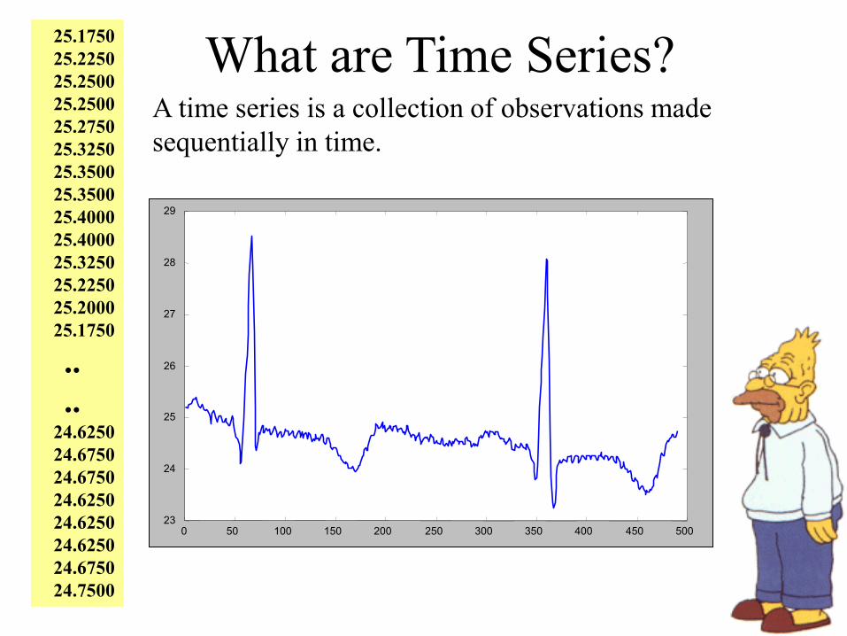
A time series is a collection of observations made
sequentially in time.

Time Series are Ubiquitous! I
• Their blood pressure
• George Bush's popularity rating
• The annual rainfall in Seattle
• The value of their Google stock
• Their blood pressure
• George Bush's popularity rating
• The annual rainfall in Seattle
• The value of their Google stock
Thus time series occur in virtually every medical, scientific and businesses domain
People measure things…People measure things…
…and things change over time……and things change over time…

Text data, may best be thought of as time series…
0 1 2 3 4 5 6 7 8x 10
50
Blue: “God” -English Bible
Red: “Dios” -Spanish Bible
Gray: “El Senor” -Spanish Bible
The local frequency
of words in the Bible
The local frequency
of words in the Bible

0 10 20 30 40 50 60 70 80 90
Hand at rest
Hand moving to
shoulder level
Steady
pointing
0 10 20 30 40 50 60 70 80 90
Hand at rest
Hand moving
above holster
Hand moving
down to grasp gun
Hand moving to
shoulder level
Steady
pointing
Video data, may best be thought of as time series…
Point
Gun-Draw

Image data, may best be thought of as time series…

What do we want to do with the time series data?
Clustering Classification
Query by
ContentRule
Discovery10
s = 0.5
c = 0.3
Motif Discovery
Novelty DetectionVisualization

Time series analysis tasks
• Similarity-based tasks
– Standard clustering, classification (KNN), etc.
• Outlier detection
• Frequent patterns (Motifs)
• Prediction

All these problems require similarity matching
Clustering Classification
Query by
ContentRule
Discovery10
s = 0.5
c = 0.3
Motif Discovery
Novelty DetectionVisualization

What is Similarity?The quality or state of being similar; likeness;
resemblance; as, a similarity of features.
Similarity is hard to
define, but…
“We know it when we
see it”
The real meaning of
similarity is a
philosophical question.
We will take a more
pragmatic approach.
Webster's Dictionary

Here is a simple motivation for the first part of the tutorial
You go to the doctor
because of chest pains.
Your ECG looks
strange…
You doctor wants to
search a database to find
similar ECGs, in the
hope that they will offer
clues about your
condition...
Two questions:• How do we define similar?
• How do we search quickly?

Two Kinds of SimilaritySimilarity at the level of
shapeNext 40 minutes
Similarity at the level of
shapeNext 40 minutes
Similarity at the structural
levelAnother 10 minutes
Similarity at the structural
levelAnother 10 minutes
time series

n
i
iicqCQD
1
2
,
Q
C
D(Q,C)
Euclidean Distance Metric
About 80% of published work in data mining uses Euclidean distance
About 80% of published work in data mining uses Euclidean distance
Given two time series:
Q = q1…qn C = c1…cn
time
1 n
time
1 n
Same meaning as in transaction data:• schema: <age, height, income, tenure>
• T1 = < 56, 176, 110, 95 >
• T2 = < 36, 126, 180, 80 >
D(T1,T2) = sqrt [ (56-36)2 + (176-126)2 + (110-180)2 + (95-80)2 ]

In the next few slides we will discuss the 4 most
common distortions, and how to remove them
In the next few slides we will discuss the 4 most
common distortions, and how to remove them
Preprocessing the data before distance calculations
• Offset Translation
• Amplitude Scaling
• Linear Trend
• Noise
Euclidean distance is very sensitive to some “distortions” in the data. For most problems these distortions are not meaningful => should remove them
Euclidean distance is very sensitive to some “distortions” in the data. For most problems these distortions are not meaningful => should remove them
If we naively try to measure the distance between two “raw” time series, we may get
very unintuitive results
If we naively try to measure the distance between two “raw” time series, we may get
very unintuitive results
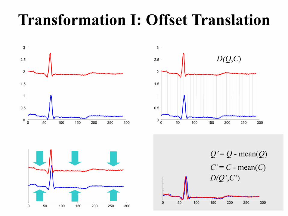
Transformation I: Offset Translation
0 50 100 150 200 250 3000
0.5
1
1.5
2
2.5
3
0 50 100 150 200 250 3000
0.5
1
1.5
2
2.5
3
0 50 100 150 200 250 3000 50 100 150 200 250 300
Q’ = Q - mean(Q)
C’ = C - mean(C)
D(Q,C)
D(Q’,C’)

Transformation II: Amplitude Scaling
0 100 200 300 400 500 600 700 800 900 1000 0 100 200 300 400 500 600 700 800 900 1000
Q’’ = (Q - mean(Q)) / std(Q)
C’’ = (C - mean(C)) / std(C)
D(Q’’,C’’)Z-score of Q
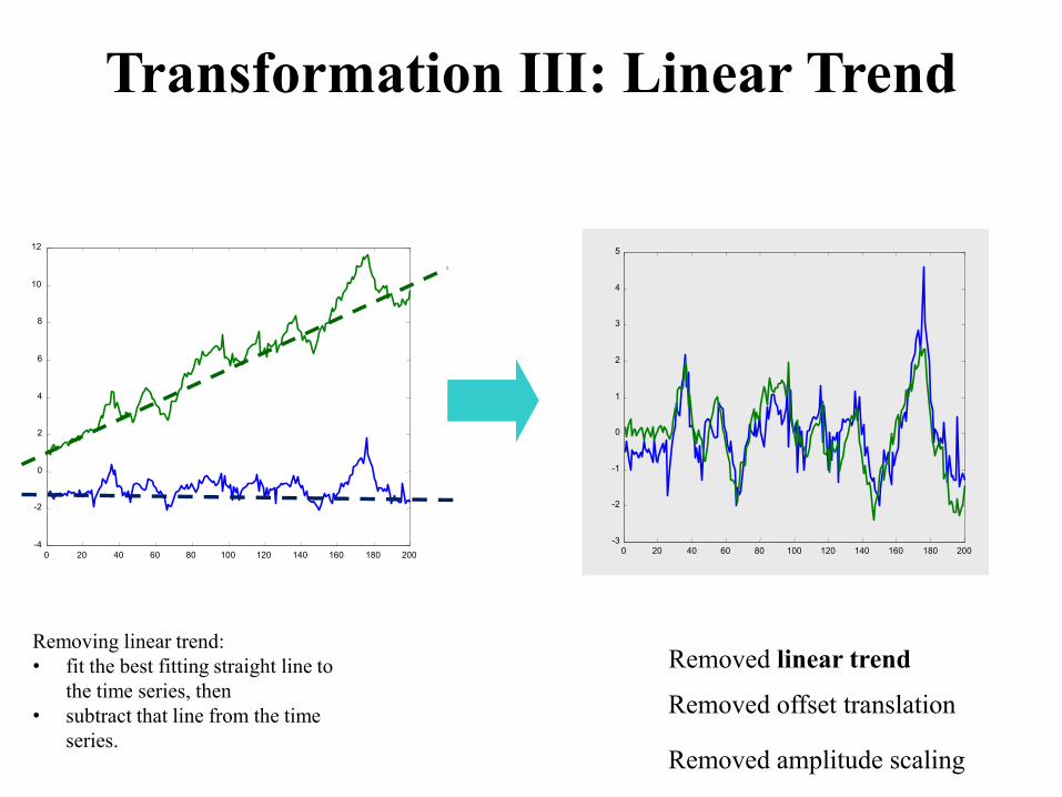
Transformation III: Linear Trend
0 20 40 60 80 100 120 140 160 180 200
-4
-2
0
2
4
6
8
10
12
0 20 40 60 80 100 120 140 160 180 200-3
-2
-1
0
1
2
3
4
5
Removed offset translation
Removed amplitude scaling
Removed linear trendRemoving linear trend:
• fit the best fitting straight line to
the time series, then
• subtract that line from the time
series.
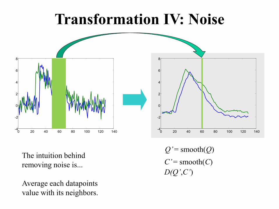
Transformation IV: Noise
0 20 40 60 80 100 120 140-4
-2
0
2
4
6
8
0 20 40 60 80 100 120 140-4
-2
0
2
4
6
8
Q’ = smooth(Q)
C’ = smooth(C)
D(Q’,C’)
The intuition behind
removing noise is...
Average each datapoints
value with its neighbors.

1
2
3
4
6
5
7
8
9
A Quick Experiment to Demonstrate the
Utility of Preprocessing the Data
1
4
7
5
8
6
9
2
3
Clustered using Euclidean distance on “clean” data.
(removing noise, linear trend, offset translation and amplitude scaling)
Clustered using Euclidean distance on “clean” data.
(removing noise, linear trend, offset translation and amplitude scaling)
Clustered using Euclidean distance on the raw data.
Clustered using Euclidean distance on the raw data.
Summary of Preprocessing
Of course, sometimes the distortions are the most interesting thing about the data, the above is only a general rule
Of course, sometimes the distortions are the most interesting thing about the data, the above is only a general rule
The “raw” time series may have distortions which we should remove before clustering, classification etc
The “raw” time series may have distortions which we should remove before clustering, classification etc
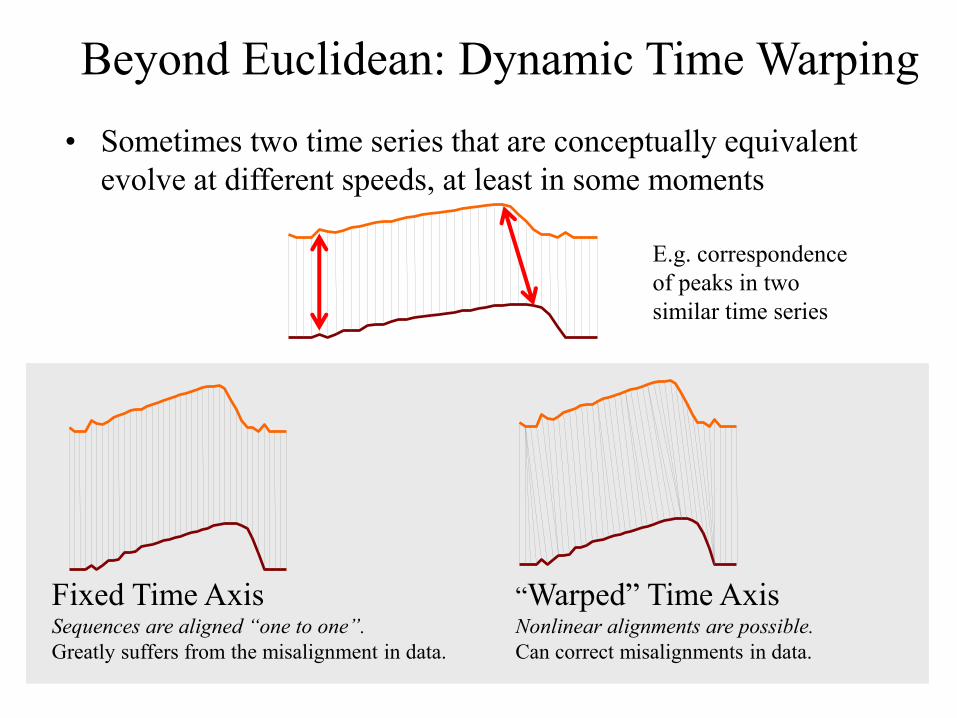
Fixed Time AxisSequences are aligned “one to one”.
Greatly suffers from the misalignment in data.
“Warped” Time AxisNonlinear alignments are possible.
Can correct misalignments in data.
Beyond Euclidean: Dynamic Time Warping
• Sometimes two time series that are conceptually equivalent
evolve at different speeds, at least in some moments
E.g. correspondence
of peaks in two
similar time series

Euclidean Dynamic Time Warping
Nuclear Power
Excellent!
Nuclear Power
Excellent!
Here is another example on nuclear power plant trace data, to help you develop an intuition
for DTW
Here is another example on nuclear power plant trace data, to help you develop an intuition
for DTW

Mountain GorillaGorilla gorilla beringei
Lowland GorillaGorilla gorilla graueri
DTW is needed for most natural
objects…
DTW is needed for most natural
objects…

C
Q
C
Q
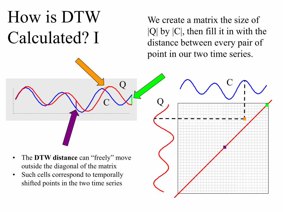
How is DTW
Calculated? I
We create a matrix the size of
|Q| by |C|, then fill it in with the
distance between every pair of
point in our two time series.
start
end
star
t
end
Time 5
Time 15
Time 30
Tim
e 5
Tim
e 1
5
Tim
e 3
0
The Euclidean distance works only on
the diagonal of the matrix
The sequence of comparisons performed:• Start from pair of points (0,0)
• After point (i,i) move to (i+1,i+1)
• End the process on (n,n)
C
QC
Q
How is DTW
Calculated? I
We create a matrix the size of
|Q| by |C|, then fill it in with the
distance between every pair of
point in our two time series.
• The DTW distance can “freely” move
outside the diagonal of the matrix
• Such cells correspond to temporally
shifted points in the two time series

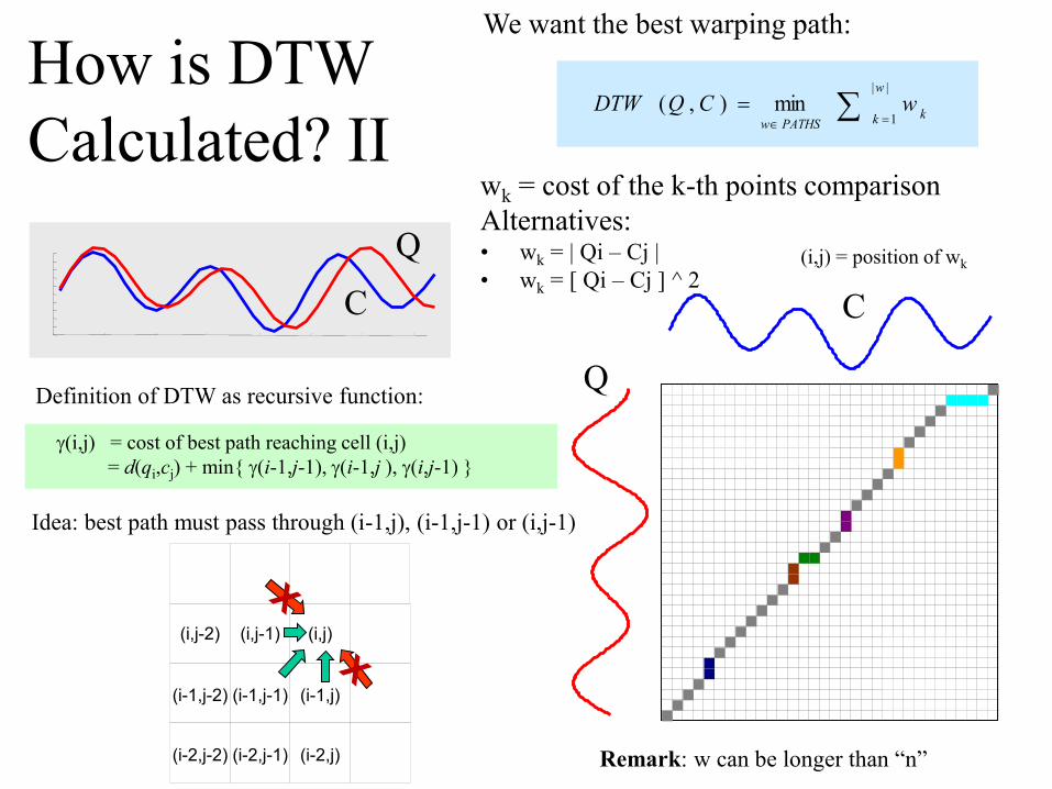
How is DTW
Calculated? II
C
Q
Warping path w
Every possible warping between two time
series, is a path though the matrix.
Euclidean distance-like parts:
Both time series move
Time warping parts:
Only one time series moves
The DTW distance can “freely” move
outside the diagonal of the matrix
The only constraints:• Start from pair of points (0,0)
• After point (i,j), either “i” or “j”
increase by one, or both of them
• End the process on (n,n)
C
Q
C
Q
How is DTW
Calculated? II
||
1min),(
w
k kPATHSw
wCQDTW
We want the best warping path:
(i,j) = cost of best path reaching cell (i,j)
= d(qi,cj) + min{ (i-1,j-1), (i-1,j ), (i,j-1) }
Definition of DTW as recursive function:
wk = cost of the k-th points comparison
Alternatives:• wk = | Qi – Cj |
• wk = [ Qi – Cj ] ^ 2
(i,j)(i,j-1)(i,j-2)
(i-1,j)(i-1,j-1)(i-1,j-2)
(i-2,j)(i-2,j-1)(i-2,j-2)
Idea: best path must pass through (i-1,j), (i-1,j-1) or (i,j-1)
(i,j) = position of wk
Remark: w can be longer than “n”
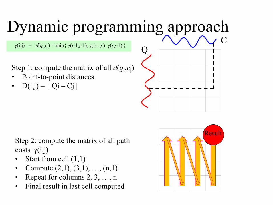
Dynamic programming approach
Step 1: compute the matrix of all d(qi,cj)
• Point-to-point distances
• D(i,j) = | Qi – Cj |
CQ
(i,j) = d(qi,cj) + min{ (i-1,j-1), (i-1,j ), (i,j-1) }
Step 2: compute the matrix of all path
costs (i,j)
• Start from cell (1,1)
• Compute (2,1), (3,1), …, (n,1)
• Repeat for columns 2, 3, …, n
• Final result in last cell computed
Result

Dynamic programming approach(i,j) = d(qi,cj) + min{ (i-1,j-1), (i-1,j ), (i,j-1) }
X X X
X X
D(1,1)
Step 2: compute the matrix of all path costs (i,j)
• Start from cell (1,1)– (1,1) = d(q1,c1) + min{ (0,0), (0,1), (1,0)}
= d(q1,c1)
= D(1,1)
• Compute (2,1), (3,1), …, (n,1)– (i,1) = d(qi,c1) + min{ (i-1,0), (i-1,1), (i,0) }
= d(qi,c1) + (i-1,1)
= D(i,1) + (i-1,1)
• Repeat for columns 2, 3, …, n– The general formula applies
+
D(i,1)
min +
D(i,1)
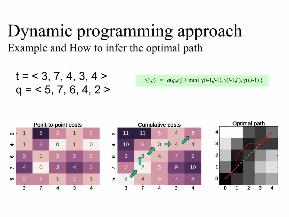
Dynamic programming approachExample and How to infer the optimal path
(i,j) = d(qi,cj) + min{ (i-1,j-1), (i-1,j ), (i,j-1) }t = < 3, 7, 4, 3, 4 >
q = < 5, 7, 6, 4, 2 >

Let us visualize the cumulative matrix on a real world problem I
This example shows 2
one-week periods from
the power demand time
series.
Note that although they
both describe 4-day work
weeks, the blue sequence
had Monday as a holiday,
and the red sequence had
Wednesday as a holiday.

Let us visualize the cumulative matrix on a real world problem II

0 10 20 30 40 50 60 70 80 900 10 20 30 40 50 60 70 80
-4
-3
-2
-1
0
1
2
3
4
Sign language
0 50 100 150 200 250 300-3
-2
-1
0
1
2
3
4
Trace
Word Spotting
Gun
Let us compare Euclidean Distance and DTW on some problems
Faces
Leaves
Control
2-Patterns
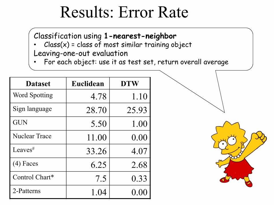
Dataset Euclidean DTW
Word Spotting 4.78 1.10
Sign language 28.70 25.93
GUN 5.50 1.00
Nuclear Trace 11.00 0.00
Leaves#33.26 4.07
(4) Faces 6.25 2.68
Control Chart* 7.5 0.33
2-Patterns 1.04 0.00
Results: Error Rate
Classification using 1-nearest-neighbor• Class(x) = class of most similar training objectLeaving-one-out evaluation• For each object: use it as test set, return overall average
Classification using 1-nearest-neighbor• Class(x) = class of most similar training objectLeaving-one-out evaluation• For each object: use it as test set, return overall average

Dataset Euclidean DTW
Word Spotting 40 8,600
Sign language 10 1,110
GUN 60 11,820
Nuclear Trace 210 144,470
Leaves 150 51,830
(4) Faces 50 45,080
Control Chart 110 21,900
2-Patterns 16,890 545,123
Results: Time (msec )
215
110
197
687
345
901
199
32
DTW is two to three
orders of magnitude
slower than
Euclidean distance
DTW is two to three
orders of magnitude
slower than
Euclidean distance
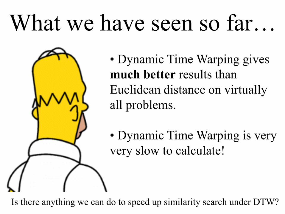
What we have seen so far…
• Dynamic Time Warping gives
much better results than
Euclidean distance on virtually
all problems.
• Dynamic Time Warping is very
very slow to calculate!
Is there anything we can do to speed up similarity search under DTW?

Fast Approximations to Dynamic Time Warp Distance I
C
QC
Q
Simple Idea: Approximate the time series with some compressed or downsampled
representation, and do DTW on the new representation. How well does this work...
Simple Idea: Approximate the time series with some compressed or downsampled
representation, and do DTW on the new representation. How well does this work...
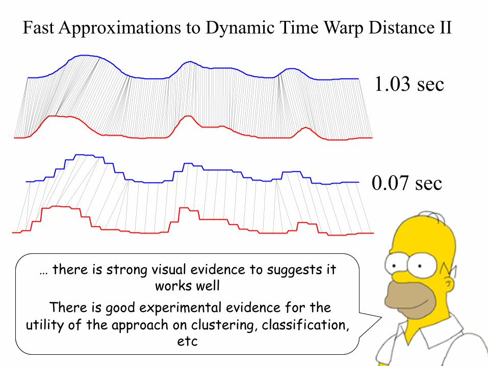
Fast Approximations to Dynamic Time Warp Distance II
0.07 sec
1.03 sec
… there is strong visual evidence to suggests it works well
There is good experimental evidence for the utility of the approach on clustering, classification,
etc
… there is strong visual evidence to suggests it works well
There is good experimental evidence for the utility of the approach on clustering, classification,
etc
C
Q
C
Q
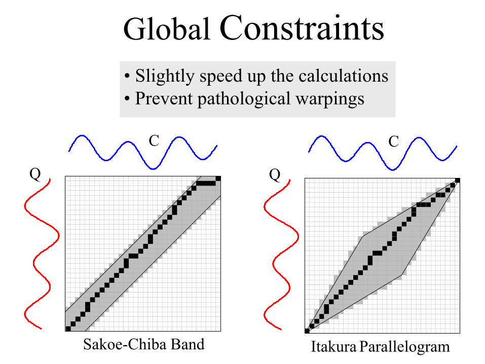
Sakoe-Chiba Band Itakura Parallelogram
Global Constraints
• Slightly speed up the calculations
• Prevent pathological warpings
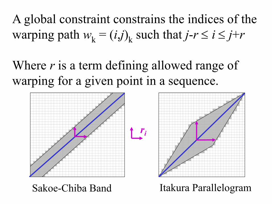
A global constraint constrains the indices of the
warping path wk = (i,j)k such that j-r i j+r
Where r is a term defining allowed range of
warping for a given point in a sequence.
ri
Sakoe-Chiba Band Itakura Parallelogram

65
70
75
80
85
90
95
100
1 5 9
13
17
21
25
29
33
37
41
45
49
53
57
61
65
69
73
77
81
85
89
93
97
10
0
FACE 2%
GUNX 3%
LEAF 8%
Control Chart 4%
TRACE 3%
2-Patterns 3%
WordSpotting 3%
Warping width that achieves
max Accuracy
Accura
cy
W: Warping Width
W
Accuracy vs. Width of Warping Window

Two Kinds of SimilarityWe are done with
shapesimilarity
We are done with
shapesimilarity
Let us considersimilarity at
the structurallevel for the
next 10 minutes
Let us considersimilarity at
the structurallevel for the
next 10 minutes
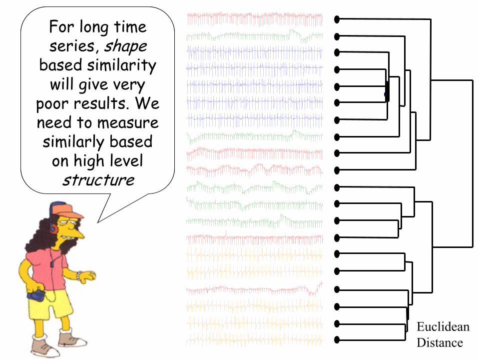
Euclidean
Distance
For long time series, shape
based similarity will give very
poor results. We need to measure similarly based on high level
structure
For long time series, shape
based similarity will give very
poor results. We need to measure similarly based on high level
structure
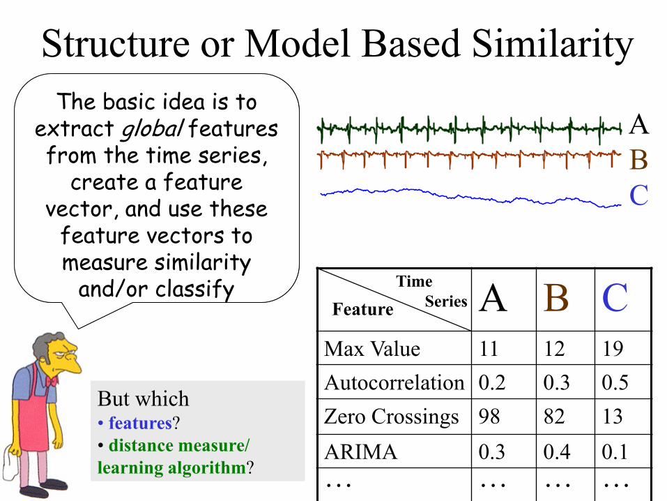
Structure or Model Based Similarity
A
B
C
A B CMax Value 11 12 19
Autocorrelation 0.2 0.3 0.5
Zero Crossings 98 82 13
ARIMA 0.3 0.4 0.1
… … … …
Feature
Time
Series
The basic idea is to extract global features from the time series,
create a feature vector, and use these
feature vectors to measure similarity
and/or classify
The basic idea is to extract global features from the time series,
create a feature vector, and use these
feature vectors to measure similarity
and/or classify
But which• features?
• distance measure/
learning algorithm?
But which• features?
• distance measure/
learning algorithm?
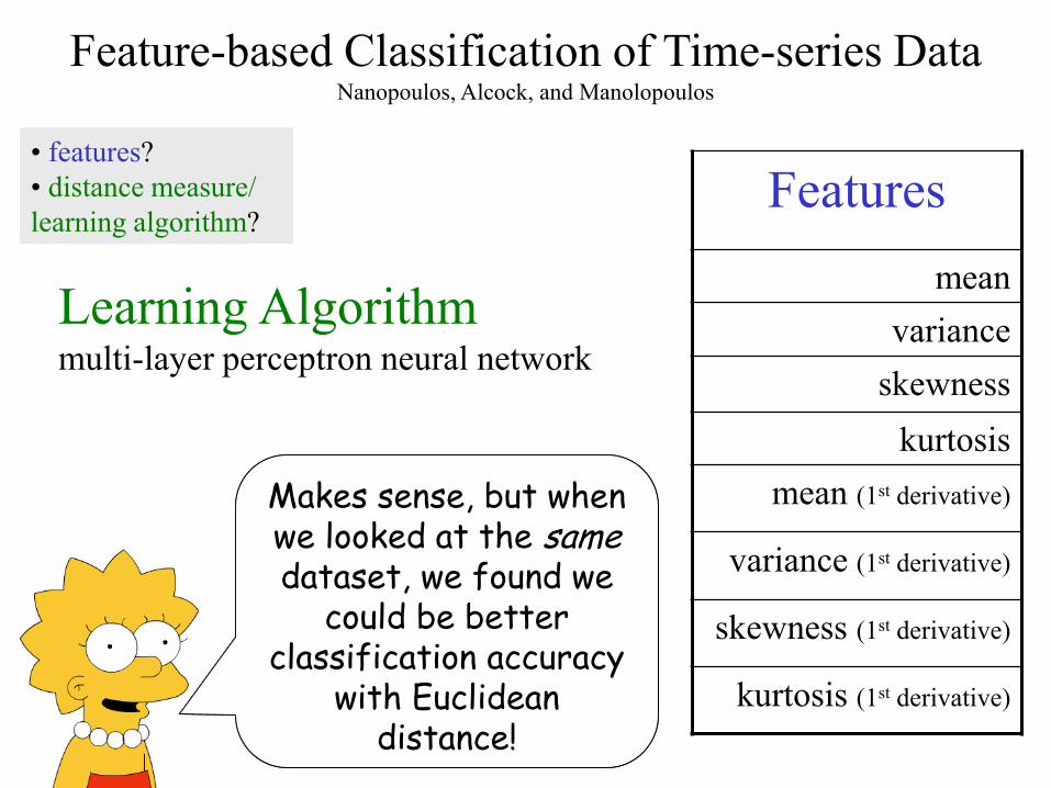
Feature-based Classification of Time-series DataNanopoulos, Alcock, and Manolopoulos
Features
mean
variance
skewness
kurtosis
mean (1st derivative)
variance (1st derivative)
skewness (1st derivative)
kurtosis (1st derivative)
Learning Algorithmmulti-layer perceptron neural network
• features?
• distance measure/
learning algorithm?
• features?
• distance measure/
learning algorithm?
Makes sense, but when we looked at the samedataset, we found we
could be better classification accuracy
with Euclidean distance!
Makes sense, but when we looked at the samedataset, we found we
could be better classification accuracy
with Euclidean distance!

Learning to Recognize Time Series: Combining ARMA Models with
Memory-Based LearningDeng, Moore and Nechyba
Features
The parameters of the
Box Jenkins model.
More concretely, the
coefficients of the
ARMA model.
Distance MeasureEuclidean distance (between coefficients)
“Time series must be
invertible and
stationary”
• features?
• distance measure/
learning algorithm?
• features?
• distance measure/
learning algorithm?
• Use to detect drunk drivers!
• Independently rediscovered and
generalized by Kalpakis et. al. and
expanded by Xiong and Yeung
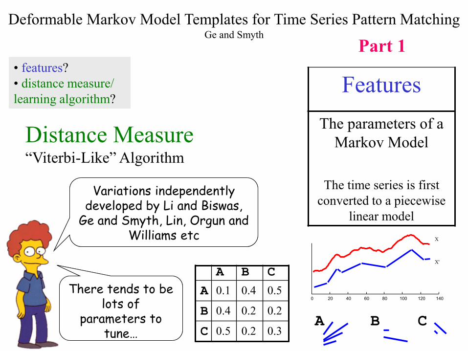
Deformable Markov Model Templates for Time Series Pattern MatchingGe and Smyth
Features
The parameters of a
Markov Model
The time series is first
converted to a piecewise
linear model
Distance Measure“Viterbi-Like” Algorithm
• features?
• distance measure/
learning algorithm?
• features?
• distance measure/
learning algorithm?
0 20 40 60 80 100 120 140
X
X'
A B C
A B C
A 0.1 0.4 0.5
B 0.4 0.2 0.2
C 0.5 0.2 0.3
Variations independently developed by Li and Biswas,
Ge and Smyth, Lin, Orgun and Williams etc
Variations independently developed by Li and Biswas,
Ge and Smyth, Lin, Orgun and Williams etc
There tends to be lots of
parameters to tune…
There tends to be lots of
parameters to tune…
Part 1

Deformable Markov Model Templates for Time Series Pattern MatchingGe and Smyth
Features
The parameters of a
Markov Model
The time series is first
converted to a piecewise
linear model
On this problem the approach
gets 98% classification accuracy*…
On this problem the approach
gets 98% classification accuracy*…
Part 2
0 50 100 150 200 250-2
-1
0
1
2
3
4
5
6
But Euclidean distance gets 100%! And has no
parameters to tune, and is tens of thousands
times faster...
But Euclidean distance gets 100%! And has no
parameters to tune, and is tens of thousands
times faster...
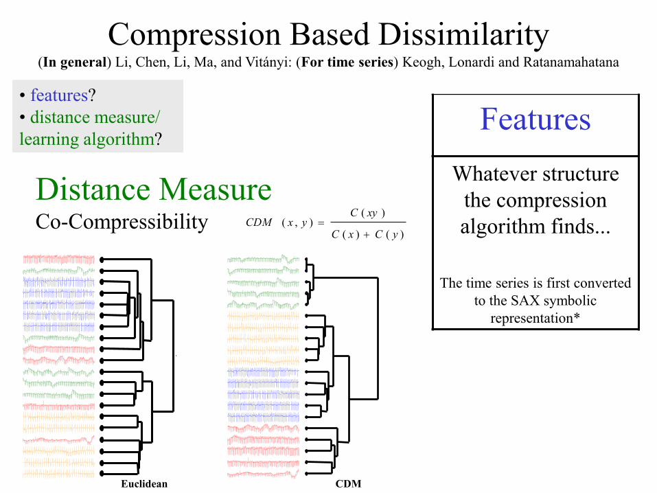
Compression Based Dissimilarity(In general) Li, Chen, Li, Ma, and Vitányi: (For time series) Keogh, Lonardi and Ratanamahatana
Features
Whatever structure
the compression
algorithm finds...
The time series is first converted
to the SAX symbolic
representation*
Distance MeasureCo-Compressibility
• features?
• distance measure/
learning algorithm?
• features?
• distance measure/
learning algorithm?
Euclidean CDM
)()(
)(),(
yCxC
xyCyxCDM

Compression Based Dissimilarity
Power : Jan-March (Italian)
Power : April-June (Italian)
Power : Jan-March (Dutch)
Power : April-June (Dutch)
Balloon1
Balloon2 (lagged)
Foetal ECG abdominal
Foetal ECG thoracic
Exchange Rate: Swiss Franc
Exchange Rate: German Mark
Sunspots: 1749 to 1869
Sunspots: 1869 to 1990
Buoy Sensor: North Salinity
Buoy Sensor: East Salinity
Great Lakes (Erie)
Great Lakes (Ontario)
Furnace: heating input
Furnace: cooling input
Evaporator: feed flow
Evaporator: vapor flow
Ocean 1
Ocean 2
Dryer fuel flow rate
Dryer hot gas exhaust
Koski ECG: Slow 1
Koski ECG: Slow 2
Koski ECG: Fast 1
Koski ECG: Fast 2
Reel 2: Angular speed
Reel 2: Tension
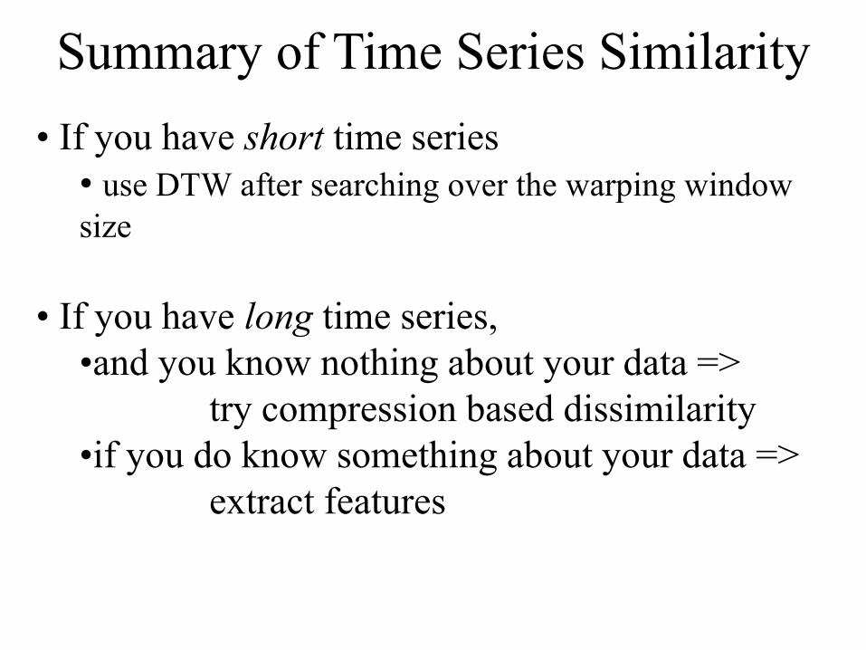
Summary of Time Series Similarity
• If you have short time series
• use DTW after searching over the warping window
size
• If you have long time series,
•and you know nothing about your data =>
try compression based dissimilarity
•if you do know something about your data =>
extract features

Time series analysis tasks
• Similarity-based tasks
– Standard clustering, classification (KNN), etc.
• Outlier detection
• Frequent patterns (Motifs)
• Prediction
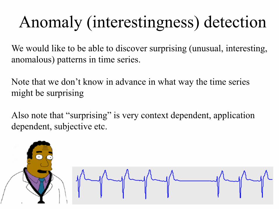
Anomaly (interestingness) detection
We would like to be able to discover surprising (unusual, interesting,
anomalous) patterns in time series.
Note that we don’t know in advance in what way the time series
might be surprising
Also note that “surprising” is very context dependent, application
dependent, subjective etc.

0 100 200 300 400 500 600 700 800 900 1000-10
-5
0
5
10
15
20
25
30
35
Limit Checking• Outliers = values outside pre-defined boundaries
– E.g. critical temperatures
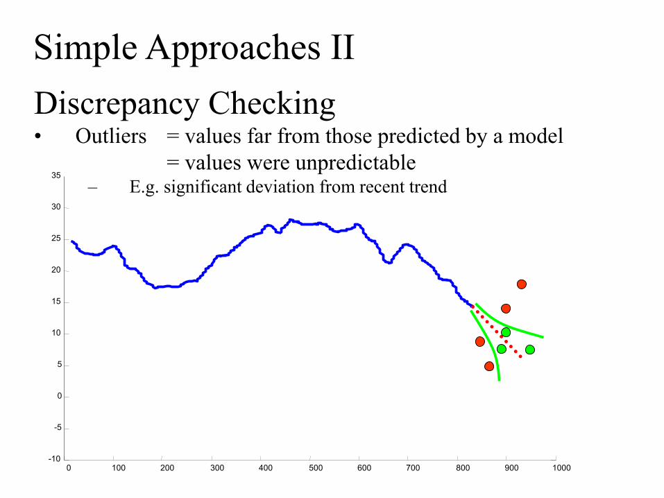
Simple Approaches I
0 100 200 300 400 500 600 700 800 900 1000-10
-5
0
5
10
15
20
25
30
35
Discrepancy Checking• Outliers = values far from those predicted by a model
= values were unpredictable– E.g. significant deviation from recent trend
Simple Approaches II

Early statistical
detection of anthrax
outbreaks by tracking
over-the-counter
medication sales
Goldenberg, Shmueli,
Caruana, and Fienberg
Discrepancy Checking: ExampleSimple averaging predictor
normalized sales
de-noised
threshold
Actual value
Predicted value
The actual value is
greater than the predicted
value, but still less than
the threshold, so no alarm
is sounded.
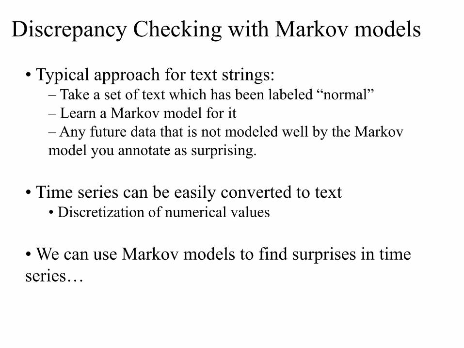
• Typical approach for text strings: – Take a set of text which has been labeled “normal”
– Learn a Markov model for it
– Any future data that is not modeled well by the Markov
model you annotate as surprising.
• Time series can be easily converted to text• Discretization of numerical values
• We can use Markov models to find surprises in time
series…
Discrepancy Checking with Markov models
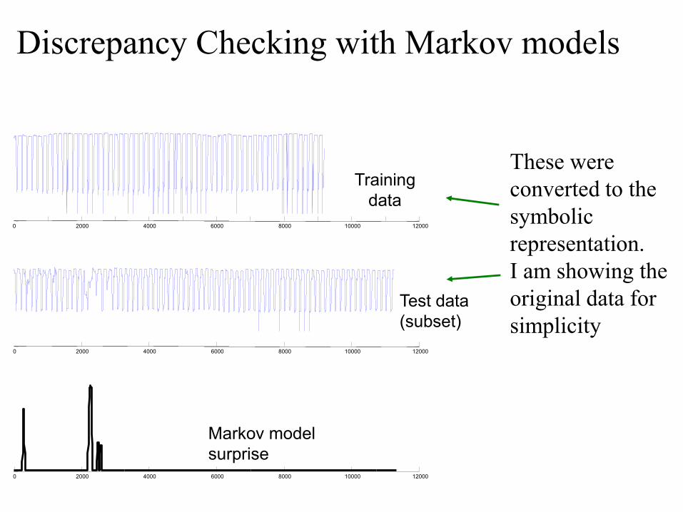
0 2000 4000 6000 8000 10000 12000
0 2000 4000 6000 8000 10000 12000
0 2000 4000 6000 8000 10000 12000
Training
data
Test data
(subset)
Markov model
surprise
These were
converted to the
symbolic
representation.
I am showing the
original data for
simplicity
Discrepancy Checking with Markov models
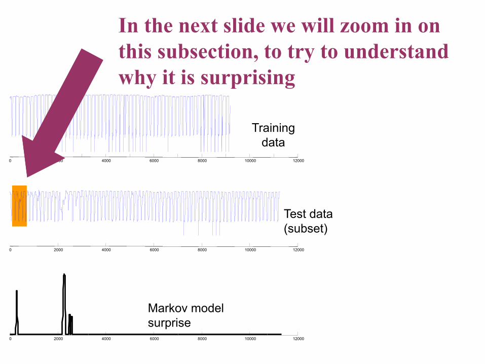
0 2000 4000 6000 8000 10000 12000
0 2000 4000 6000 8000 10000 12000
0 2000 4000 6000 8000 10000 12000
Training
data
Test data
(subset)
Markov model
surprise
In the next slide we will zoom in on
this subsection, to try to understand
why it is surprising
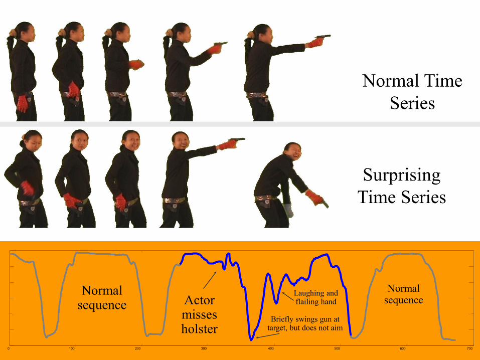
0 100 200 300 400 500 600 700
Normal sequence
Normal sequenceActor
misses holster
Briefly swings gun at target, but does not aim
Laughing and flailing hand
Normal Time
Series
Surprising
Time Series
Anomaly (interestingness) detection
In spite of the nice example in the previous slide, the
anomaly detection problem is wide open.
How can we find interesting patterns…
• Without (or with very few) false positives…
• In truly massive datasets...
• In the face of concept drift…
• With human input/feedback…
• With annotated data…

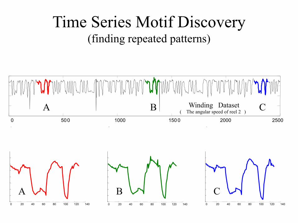
Time Series Motif Discovery (finding repeated patterns)
Winding Dataset( The angular speed of reel 2 )
0 500 1000 150 0 2000 2500
Are there any repeated patterns, of about this length in the above time series?
Are there any repeated patterns, of about this length in the above time series?
Winding Dataset( The angular speed of reel 2 )
0 500 1000 150 0 2000 2500
0 20 40 60 80 100 120 140 0 20 40 60 80 100 120 140 0 20 40 60 80 100 120 140
A B C
A B C
Time Series Motif Discovery (finding repeated patterns)

· Mining association rules in time series requires the discovery of motifs.
These are referred to as primitive shapes and frequent patterns.
· Several time series classification algorithms work by constructing typical
prototypes of each class. These prototypes may be considered motifs.
· Many time series anomaly/interestingness detection algorithms essentially
consist of modeling normal behavior with a set of typical shapes (which we see
as motifs), and detecting future patterns that are dissimilar to all typical shapes.
· In robotics, Oates et al., have introduced a method to allow an autonomous
agent to generalize from a set of qualitatively different experiences gleaned
from sensors. We see these “experiences” as motifs.
· In medical data mining, Caraca-Valente and Lopez-Chavarrias have
introduced a method for characterizing a physiotherapy patient’s recovery
based of the discovery of similar patterns. Once again, we see these “similar
patterns” as motifs.
• Animation and video capture… (Tanaka and Uehara, Zordan and Celly)
Why Find Motifs?

Definition 1. Match: Given a positive real number R (called range) and a time series T containing a
subsequence C beginning at position p and a subsequence M beginning at q, if D(C, M) R, then M is
called a matching subsequence of C.
Definition 2. Trivial Match: Given a time series T, containing a subsequence C beginning at position
p and a matching subsequence M beginning at q, we say that M is a trivial match to C if either p = q
or there does not exist a subsequence M’ beginning at q’ such that D(C, M’) > R, and either q < q’< p
or p < q’< q.
Definition 3. K-Motif(n,R): Given a time series T, a subsequence length n and a range R, the most
significant motif in T (hereafter called the 1-Motif(n,R)) is the subsequence C1 that has highest count
of non-trivial matches (ties are broken by choosing the motif whose matches have the lower
variance). The Kth most significant motif in T (hereafter called the K-Motif(n,R) ) is the subsequence
CK that has the highest count of non-trivial matches, and satisfies D(CK, Ci) > 2R, for all 1 i < K.
0 100 200 3 00 400 500 600 700 800 900 100 0
T
Space Shuttle STS - 57 Telemetry( Inertial Sensor )
Trivial
Matches
C

OK, we can define motifs, but
how do we find them?
The obvious brute force search algorithm is just too slow…
Many algorithms realized, main ones are based on random
projection* and SAX discretized representation of times
series (useful to compute quick lower bound distances).
* J Buhler and M Tompa. Finding motifs using
random projections. In RECOMB'01. 2001.
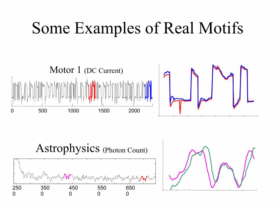
Some Examples of Real Motifs
0 500 1000 1500 2000
Motor 1 (DC Current)
2500
3500
4500
5500
6500
Astrophysics (Photon Count)
Winding Dataset( The angular speed of reel 2 )
0 500 1000 150 0 2000 2500
A B C
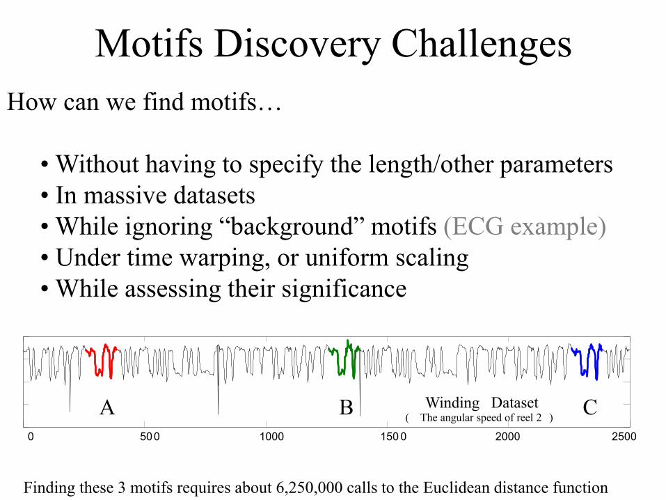
Finding these 3 motifs requires about 6,250,000 calls to the Euclidean distance function
Motifs Discovery Challenges
How can we find motifs…
• Without having to specify the length/other parameters
• In massive datasets
• While ignoring “background” motifs (ECG example)
• Under time warping, or uniform scaling
• While assessing their significance

Time Series Prediction
There are two kinds of time series prediction
• Black Box: Predict tomorrows electricity
demand, given only the last ten years
electricity demand.
• White Box (side information ): Predict
tomorrows electricity demand, given the last
ten years electricity demand and the weather
report, and the fact that fact that the world
cup final is on and…
Prediction is hard, especially about the futurePrediction is hard, especially about the future
Yogi Berra1925 - 2015

Black Box Time Series Prediction
• Very difficult task, at least in longer-term prediction
• Several solutions are claiming great results, yet they
are mostly still unreliable:
– A paper in SIGMOD 04 claims to be able to get better than 60%
accuracy on black box prediction of financial data (random guessing
should give about 50%). The authors later agreed to test blind on a
external and again got more than 60% -- though it was completely
random data (quantum-mechanical random walk)…
– A paper in SIGKDD in 1998 did black box prediction using association
rules, more than twelve papers extended the work… but then it was
proved that the approach could not work*!

End of Time series module