Universite libre de Bruxelles

Advanced Databases

Winter Semester 2017-2018

Time Series Databases

and InfluxDB

Authors:Syeda Noor Zehra Naqvi

(000455274)Sofia Yfantidou

(000456361)

Supervisor:Dr. Esteban Zimanyi

December 17, 2017

Contents

1 TIME SERIES & TIME SERIES DBs 31.1 Time Series . . . . . . . . . . . . . . . . . . . . . . . . . . . . 3

1.1.1 Definition . . . . . . . . . . . . . . . . . . . . . . . . . 31.1.2 Uses . . . . . . . . . . . . . . . . . . . . . . . . . . . . 3

1.2 Time Series Databases . . . . . . . . . . . . . . . . . . . . . . 41.2.1 Definition . . . . . . . . . . . . . . . . . . . . . . . . . 41.2.2 Properties . . . . . . . . . . . . . . . . . . . . . . . . . 41.2.3 Popularity . . . . . . . . . . . . . . . . . . . . . . . . . 51.2.4 Benefits and Uses . . . . . . . . . . . . . . . . . . . . . 61.2.5 Top Time Series Databases . . . . . . . . . . . . . . . . 7

2 INFLUXDB 82.1 General Information & Architecture . . . . . . . . . . . . . . . 8

2.1.1 Key Concepts . . . . . . . . . . . . . . . . . . . . . . . 92.1.2 Sharding . . . . . . . . . . . . . . . . . . . . . . . . . . 112.1.3 Storage Engine . . . . . . . . . . . . . . . . . . . . . . 12

2.2 Customers & Use Cases . . . . . . . . . . . . . . . . . . . . . 122.2.1 DevOps Monitoring: The IBM Case . . . . . . . . . . . 132.2.2 IoT Monitoring: The Spiio Case . . . . . . . . . . . . . 132.2.3 Real-Time Analytics: The eBay Case . . . . . . . . . . 14

2.3 Pros & Cons . . . . . . . . . . . . . . . . . . . . . . . . . . . . 142.3.1 Pros . . . . . . . . . . . . . . . . . . . . . . . . . . . . 142.3.2 Cons . . . . . . . . . . . . . . . . . . . . . . . . . . . . 162.3.3 When not to use InfluxDB . . . . . . . . . . . . . . . . 17

2.4 Popularity . . . . . . . . . . . . . . . . . . . . . . . . . . . . . 172.5 Comparisons . . . . . . . . . . . . . . . . . . . . . . . . . . . . 18

3 HANDS-ON WORK 183.1 Dataset Presentation . . . . . . . . . . . . . . . . . . . . . . . 183.2 InfluxDB Tutorial . . . . . . . . . . . . . . . . . . . . . . . . . 21

3.2.1 Database Setup . . . . . . . . . . . . . . . . . . . . . . 213.2.2 Schema Design . . . . . . . . . . . . . . . . . . . . . . 213.2.3 Data Import . . . . . . . . . . . . . . . . . . . . . . . . 223.2.4 Basic Queries . . . . . . . . . . . . . . . . . . . . . . . 24

3.3 Benchmarking SQL Server vs InfluxDB . . . . . . . . . . . . . 283.3.1 Query Properties . . . . . . . . . . . . . . . . . . . . . 28

1

3.3.2 Hardware Specifications . . . . . . . . . . . . . . . . . 293.3.3 Benchmarking Queries . . . . . . . . . . . . . . . . . . 303.3.4 Benchmarking Query Results . . . . . . . . . . . . . . 32

3.4 Benchmarking . . . . . . . . . . . . . . . . . . . . . . . . . . . 363.4.1 InfluxDB vs. Cassandra . . . . . . . . . . . . . . . . . 363.4.2 InfluxDB vs. Elasticsearch . . . . . . . . . . . . . . . . 383.4.3 InfluxDB vs. OpenTSDB . . . . . . . . . . . . . . . . . 41

2

1 TIME SERIES & TIME SERIES DBs

1.1 Time Series

1.1.1 Definition

“Time Series is an ordered sequence of values of a variable (e.g.temperature)at equally spaced time intervals (e.g. hourly).” Thus it is a sequence ofdiscrete-time data. For instance timestamped data, such as log files and IoTdevices’ measurements can be considered time series. The measurements thatconstitute a time series are ordered on a timeline, which reveals informationabout underlying patterns. Ordering matters, because there is a dependencybetween time and measurements and changing the order could change themeaning of the data [4]. Example time series would be the hourly measure-ments of temperature at a specific weather station, daily measurements ofthe closing price of a specific stock, etc.

1.1.2 Uses

Time series are used in various context, the most common of them being1:

• Time Series Analysis: Time Series Analysis is utilized in order toexplore how a given variable changes over time. For instance CensusAnalysis, namely public opinion analysis on a specific matter over time,e.g. presidential candidates in U.S. elections, can be considered a TimeSeries Analysis task.

• Regression Analysis: Regression Analysis can be utilized to examinehow the changes associated with a specific variable can cause shifts inother variables over the same time period. For instance, Stock MarketAnalysis, namely how one stock’s prices over time affect other stocks’prices or unemployment over the same time period, can be considereda Regression Analysis task.

• Time Series Forecasting: Time Series Forecasting uses informationregarding historical values and associated patterns to predict futureactivity. For example, Economic Forecasting, Weather Forecasting,Earthquake Forecasting (seismic time series), Sales Forecasting, etc.

1Time Series - Investopedia. 2017. Retrieved from http://www.investopedia.com/

terms/t/timeseries.asp.

3

1.2 Time Series Databases

1.2.1 Definition

A Time Series Database (TSDB) is a database type which is optimized fortime series or time-stamped data. It is built specifically for handling metrics,events or measurements that are time-stamped. A TSDB is optimized formeasuring change over time. A TSDB allows its users to create, enumerate,update, destroy and organize various time series in a more efficient manner.The key difference with time series data from regular data is that mostly youask questions about it over time. Nowadays, the majority of the companiesare generating a insanely large stream of metrics and events (time series data)and hence the need of a TSDBs is unavoidable.

1.2.2 Properties

The main properties distinguishing time series data from the regular dataworkloads are summarization, data life cycle management, and large rangescans of many records. The overview of some of the required properties of aTSDB is as follows:

• Data Location: If related data is not located together in the physicalstorage, the data queries can be really slow and even result in timeoutsbecause non-sequential I/O operations are still very slow as comparedto the sequential I/O even when using SSD. A TSDB co-locates chucksof data within the same time range on the same physical part of thedatabase cluster and hence enables quick access for faster, more efficientanalysis.

• Fast, easy range queries: As a TSDB keeps the co-related datatogether it ensures that the range queries are fast. In many cases regulardatabases produce an index out of memory error because of the sheervolume of time series data and subsequently affect the performanceof read and write operations. In addition, it should be taken intoconsideration that the query language used should make it easier forusers to write such queries.

• High write performance: A lot of databases are not able to serverequests predictably and quickly during peak loads. TSDBs shouldensure high availability and high performance for both read and write

4

operations during peak loads because they are usually designed to stayavailable even under the most demanding conditions. Time series datais usually being recorded every second or even less than that, so writeoperations need to be fast.

• Data compression: As time-series data is mostly recorded per secondor even with less granularity, they usually need a better data compres-sion technique. And as the data grows older granularity becomes lessimportant, so TSDBs should provide functionality to perform roll-upsin such scenarios for data compaction.

• Scalability: Time-series data increases very quickly. For example aconnected car will send 25 GB of data to the cloud every hour2. Andregular databases are not designed to handle this scalability. On theother hand time series databases are designed to take care of scale byintroducing functionalities that are only possible when you treat timeas your first concern. This can result in performance improvements,including: higher insertion rates, faster queries at scale, and betterdata compression.

• Usability: TSDBs typically include functions and operations that arecommon to time series data analysis. For example they utilize dataretention policies, continuous queries, flexible time aggregations, rangequeries etc. So this increases the usability by improving the user expe-rience in case of dealing with time related analysis.

1.2.3 Popularity

It is obvious that TSDBs are to handle time series data, but their popular-ity seems to have increased with the emergence of Internet of things (IoT).IoT is a network of physical devices/objects with connectivity which enablesthem to exchange and collect data. Such technologies are generating largeamount of data which is usually time-stamped, so with the increase in pop-ularity of IoT, TSDBs popularity increased even more, because they can beused to efficiently store sensors and devices’ data in this domain. Some othercommon uses of TSDBs are DevOps monitoring and real time data analy-sis. Nowadays, many large companies like Facebook, eBay etc. are using

2Quartz Media. More details here: https://qz.com/344466/

connected-cars-will-send-25-gigabytes-of-data-to-the-cloud-every-hour/.

5

TSDBs instead of relational databases especially for data monitoring pur-poses. From the graph in Figure 1a it can be seen that the popularity ofTSDBs is increasing rapidly in the past couple of years. From 2015 to 2016the popularity of TSDBs in increased by 26.7% which is twice as much asGraph database management systems which is 2nd in the list. The popular-ity of TSDBs continues to increase till now. In Figure 1b we visualize theincrease in popularity of IoT starting from 2015 as well, to give an idea ofthe simultaneous grow of the two fields.

(a) DB-Engines Ranking, PopularityTrend (Source: https://www.db-engines.com).

(b) Sketching out the Internet ofThings trendline, Brookings (Source:https://www.brookings.edu/).

Figure 1: Popularity Charts for TSDBs and IoT.

1.2.4 Benefits and Uses

As mentioned earlier Section 1.2.3, some common applications of TSDBsare IoT, DevOps, Data Analytics etc. But the question is that why do weprefer TSDBs over normal databases in such applications? Some additionaladvantages of using TSDBs are as follows:3

• Massive scalability and performance: It can be predicted fromthe TSDB properties described in Section 1.2.3 that an efficient andgood TSDB allows an application to scale easily to support millions of

3Benefits of a TSDB. Retrieved fromhttp://basho.com/resources/

time-series-databases/.

6

IoT devices or time series data points in a continuous flow and performreal-time analysis.

• Reduced downtime: In real life scenarios there are some situationswhere availability is critical at all times, the architecture of a databasethat is built for time series data avoids any downtime for data even inthe event of network partitions or hardware failures.

• Lower costs: Flexibility and high threshold to failure translates intofewer resources needed to manage outages. Commodity hardware usedfor fast and easy scaling ensures the reduction of operational and hard-ware costs of scaling up or down.

• Improved business decisions: As TSDB enables an organization tomonitor and analyze data in real time, it helps it in making faster andmore accurate adjustments for infrastructure changes, consumption ofenergy, device maintenance or other major decisions that influence thebusiness.

Some use cases for TSDBs includes monitoring software systems like virtualmachines, different services or applications, monitoring physical systems forexample some equipment or machines, connected devices, the environment,home management systems, human bodies etc. Another use of TSDBs isin financial trading systems for classic securities or in crypto currencies (bitcoins etc). TSDBs can also be used as eventing applications for trackinguser/customer interaction data and in business intelligence tools for trackingkey metrics and the general health of the business.

1.2.5 Top Time Series Databases

Top few TSDBs and their ranking can be seen in the Figure 2 according toDB-Engines Ranking of Time Series DBMS. DB-Engines [1] is an indepen-dent website which ranks databases based on search engine popularity, socialmedia mentions, number of job offers, and technical discussion frequency.Influx DB is ranked number one in this list as of October 2017. Figure 2also shows the historical changes of these databases and it can be seen thatInfluxDB was also the top TSDB in October 2016 and it maintained it’sranking. In the following Section 2 we will discuss InfluxDB in detail. Thesecond on the list is RRDtool which is an open source, industry standard

7

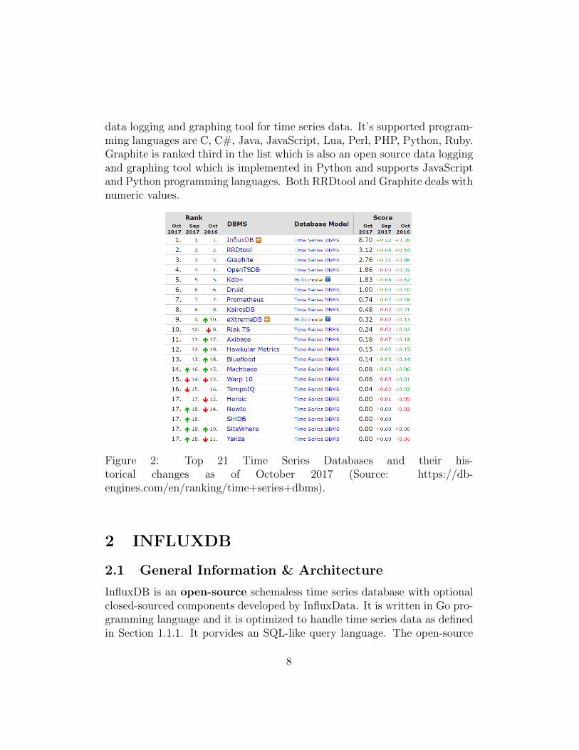
data logging and graphing tool for time series data. It’s supported program-ming languages are C, C#, Java, JavaScript, Lua, Perl, PHP, Python, Ruby.Graphite is ranked third in the list which is also an open source data loggingand graphing tool which is implemented in Python and supports JavaScriptand Python programming languages. Both RRDtool and Graphite deals withnumeric values.

Figure 2: Top 21 Time Series Databases and their his-torical changes as of October 2017 (Source: https://db-engines.com/en/ranking/time+series+dbms).

2 INFLUXDB

2.1 General Information & Architecture

InfluxDB is an open-source schemaless time series database with optionalclosed-sourced components developed by InfluxData. It is written in Go pro-gramming language and it is optimized to handle time series data as definedin Section 1.1.1. It porvides an SQL-like query language. The open-source

8

version, namely the TICK Stack (See Image 3), provides a full time seriesdatabase platform with various services including the InfluxDB core and canrun on cloud and on premises on a single node. The closed-source versions,namely InfluxEnterprise (IE) and InfluxCloud (IC), offer extra functionali-ties, such as high availability, scalability, backup and restore, and run eitheron premises (IE) or on cloud (IC). More details on the suitability of eachversion for specific use cases will be given in Section 2.3.

Figure 3: The open-source, Time Series Database Platform, TICK stack(Source: https://www.influxdata.com/time-series-platform/).

2.1.1 Key Concepts

Before we dive deeper into InfluxDB some key concepts should be defined.In order to illustrate these concepts in an easy way a simple real-life-likeexample will be utilized (See Table 1). This example is based on a similarone presented in InfluxDB’s documentation [3]. It shows the number of minorand adult passengers picked up by taxi drivers Doe and Jones at locations 1and 2 between 18/08/2015 at 00:00 and 18/08/2015 at 06:30.

First of all, the most important concept in InfluxDB is time. The timecolumn is included in every InfluxDB database and stores discrete times-tamps, which are associated with specific data. The next two columns, mi-nors and adults, are fields (another term for attributes). Each field consistsof a field key e.g. minors and a field value e.g. 1. Field values are the

9

name=passengers

time minors adults location driver

2015-08-18T00:00:00Z 1 2 1 doe

2015-08-18T00:00:00Z 2 2 1 jones

2015-08-18T00:06:00Z 1 1 1 doe

2015-08-18T00:06:00Z 0 1 1 jones

2015-08-18T05:54:00Z 0 2 2 doe

2015-08-18T06:30:00Z 2 2 2 doe

2015-08-18T06:06:00Z 3 1 2 jones

2015-08-18T06:30:00Z 0 4 2 jones

Table 1: Sample time series dataset.

actual data and are always associated with a timestamp. Each field key-fieldvalue pair is a field set. Our dataset has 8 field sets:

• minors=1, adults=2

• minors=2, adults=2

• minors=1, adults=1

• minors=0, adults=1

• minors=0, adults=2

• minors=2, adults=2

• minors=3, adults=1

• minors=0, adults=4

The location and driver columns are called tags. Again. each tag consistsof a tag key and a tag value. Each tag key-tag value pair constitutes a tagset. The following 8 tag sets are included in the dataset:

• location=1, driver=doe

• location=1, driver=jones

• location=1, driver=doe

• location=1, driver=jones

• location=2, driver=doe

• location=2, driver=doe

• location=2, driver=jones

• location=2, driver=jones

The difference between tags and fields is that tags are indexed, whichmeans than queries on tags are faster compared to queries on simple fields,which are not indexed. Note that the primary key consists of the timestamp

10

Series Number Retention Policy Measurement Tag set

Series 1 autogen passengers location=1, driver=doe

Series 2 autogen passengers location=1, driver=jones

Series 3 autogen passengers location=2, driver=doe

Series 4 autogen passengers location=2, driver=jones

Table 2: The series that constitute our dataset.

and the tags. Another important concept is measurement (think of it asan SQL table). The measurement technically explains our fields’ content. Inother words the minors and adults columns in our table contain the numberof passengers (See name in the 1st row of Table 1) and not their years,height, etc. A single measurement can belong to different retention policies.A retention policy describes how long InfluxDB stores data (DURATION)and how many copies of those data are stored in the cluster. The defaultretention policy with infinite duration and no replication is called autogen,which has an infinite duration and a replication factor on 1. Maybe the mostimportant concept in InfluxDB is series, which is a collection of data withcommon retention policy, measurement and tag set. A point is is the field setin the same series with a specific timestamp e.g.time=2015-08-18T00:00:00Z,minors=1, adults=2, location=1, driver=doe. Our dataset consists of 4 seriesas shown in Table 2.

2.1.2 Sharding

Sharding is the horizontal partitioning of data in a database. Each partitionis called shard. InfluxDB stores data in shard groups, which are organizedby retention policy and store data with timestamps that fall within a specifictime interval. The length of the aforementioned time interval depends on theduration of the retention policy (RP). The default shard group durations are1 hour for RP less than 2 days, 1 day for RP between 2 days and 6 monthsand 7 days for RP greater than 6 months. The duration of the shard groupis important for efficient drop operations, where data is dropped per shard,not per data point. For instance if a RP has a duration of 10 hours, it makesno sense to divide the data in 5-hour intervals. However, short shard groupdurations for large RP can harm compression and speed. Recommendationfor appropriate sharding and schema design can be found here.

11

2.1.3 Storage Engine

InfluxDB currently uses its in-house built data structure, the Time Struc-tured Merge Tree (TSM Tree). More details on this storage format willbe given shortly. However, InfluxDB has utilized various storage formatsover different versions. Initially it used LevelDB (a database based on LogStructured Merge Trees (LSM)), which optimizes write throughput and of-fers built-in compression. However, LevelDB does not provide hot backupfunctionality, which means you need to close the database to safely copy it.For this reason InfluxDB utilized LevelDB variants, such as RocksDB andHyperLevelDB, which also use LSM Trees. There is an inherent problemwith LSM Trees though, deletion is an expensive operation and a time seriesDB requires deletions on a large scale due to automatic data retention (SeeSection 2.1.1). That’s why InfluxDB switched to an alternative data struc-ture, the mmap B+Tree. It used BoltDB as the underlying storage engine,which may perform slightly worse in write operations, but offers increasedstability and reliability. However, they realized that when the database be-came larger, writes would start spiking Input Output Operations per Second(IOPS). Subsequently, the InfluxDB team decided to build their own storageformat, the TSM Tree. The TSM Tree is similar to a LSM Tree in a sensethat it uses write ahead log, index files that are read only, and it occasionallyperforms compactions to combine index files. However, it does not suffer bythe deletion problem and offers better compression rates (45x improvementin disk space usage) compared to a B+ Tree4.

2.2 Customers & Use Cases

InfluxDB has more than 70000 active installs and is preferred by customersfor DevOps Monitoring (Infrastructure Monitoring, Application Monitor-ing, Cloud Monitoring), IoT Monitoring, and Real-Time Analytics. Itscustomers include, but are not limited to, AXA, Cisco, eBay, IBM and more.Customers’ success stories per category can be found below.

4The New InfluxDB Storage Engine: Time Structured Merge Tree —InfluxData. 2017. Retrieved from https://www.influxdata.com/blog/

new-storage-engine-time-structured-merge-tree/.

12

2.2.1 DevOps Monitoring: The IBM Case

“The IBM® Trusteer® products help detect and prevent the full rangeof attack vectors responsible for the majority of online, mobile and cross-channel fraud.” In order to provide full protection against online fraud atall times, the Trusteer platform needs to maintain high availability. For thispurpose its team uses DevOps monitoring techniques powered by InfluxDB,Telegraf5 (another product of the InfluxData ecosystem) and Grafana6 (open-source software for time series analytics). They use Telgraf for collectingdata, InfluxDB for storing them and Grafana for analysis and visualization.They collect data on infrastructure and application performance, in order tomonitor their cloud system, which contains hundreds of virtual servers.

2.2.2 IoT Monitoring: The Spiio Case

Spiio enables monitoring vertical living green walls and high value greenplant installations by providing sensors and the related software to horti-culturalists. Green walls are becoming more and more popular especially inlarge cities, bringing nature closer to city life. However, maintaining multiplegreen walls in a city can be a problem for horticulture professionals; that’swhy Spiio uses sensors to understand plant performance from data, and thuscut maintenance cost drastically, ensuring full digital control of millions ofplants.

Spiio tried adopting various solutions before InfluxDB, namely IoT plat-forms, such as AWS Greengrass and Azure IOT, multi-purpose databases orsearch engines, such as MySQL, Cassandra, Elasticsearch, and even time-series databases, such as OpenTSDB. However, none of these solutions wasas holistic as InfluxData. Currently, Spiio uses InfluxDB for data storage,Kapacitor7 for real-time, streaming data analytics and Chronograf8 for datavisualization. Both Kapacitor and Chronograf are part of the InfluxDataecosystem. InfluxData enables Spiio’s clients to access and share never-before possible insights on optimizing green wall maintenance by tracking

5Telegraf from InfluxData — Agent for Collecting & Reporting Metrics & Data. 2017.Retrieved from https://www.influxdata.com/time-series-platform/telegraf/.

6Grafana. 2017. Retrieved from https://grafana.com/.7Kapacitor from InfluxData — Real-time streaming data processing engine. 2017.

Retrieved from https://www.influxdata.com/time-series-platform/kapacitor/.8Chronograf from InfluxData — Complete Interface for the InfluxData Platform. 2017.

Retrieved from https://www.influxdata.com/time-series-platform/chronograf/.

13

the impact of factors that influence plant performance.

2.2.3 Real-Time Analytics: The eBay Case

EBay Inc. is a global e-commerce leader. Various teams inside eBay utilizeInfluxDB and InfluxData ecosystem in general for DevOps monitoring andreal-time analytics. Here, we will focus on real-time analytics inside eBay’sExperimentation team. This team is responsible for eBay’s experimentationplatform, which runs more than 1500 experiments9 and enables eBay’s busi-ness users to gain insight on important analytics and answer crucial businessquestions. However, experiments can experience anomalies, such as trafficcorruption, and here is where InfluxDB comes in. Anomalies are detecteddaily utilizing Anomaly/Traffic Prediction algorithms and stored into In-fluxDB and are visualized in Grafana. Having this analyzed data representedin time series format is key and allows them to present it in their Grafanadashboard. This combination enables the Experimentation platform to bescalable and self-sufficient, namely by creating new dashboards and datasetsautomatically.

2.3 Pros & Cons

2.3.1 Pros

1. Tailored-made for Time Series data: InfluxDB is designed tohandle time series data more efficiently. It is designed to have impres-sive write and read throughputs as will be discussed in Sections 2.5 and3.4.

2. Solutions for Every Need: InfluxData provides an Open-Sourcecore that includes InfluxDB, Kapacitor, Telegraf and Chronograf (theTICK Stack) free of charge. It also provides a SaaS solution, namelythe InfluxCloud, that offers high availability, scalability and advancedbackup and restore functionalities for users with bigger needs andlimited infrastructure. InfluxCloud deploys servers in the U.S.A.,Canada and Europe. There is also an in-house solution of Influx-Cloud, namely InfluxEnterprise, for customers who want to utilize their

9Monitoring Anomalies in the Experimentation Platform.2017. Retrieved from http://www.ebaytechblog.com/2016/10/06/

monitoring-anomalies-in-the-experimentation-platform/.

14

own infrastructure or cloud services. In other words, InfluxDB offersvarious solutions to match every potential business need.

3. Holistic Solution: InfluxDB is designed to work perfectly along withthe rest of the InfluxData ecosystem, namely Kapacitor, Telegraf andChronograf. In this sense it is so much more than a simpledatabase. It is part of a holistic solution that offers accumulation,analysis and visualization, all in one package.

4. Various Input Plugins: InfluxDB does not limit itself to one or twoinput methods, like other TSDBs, but it offers various input pluginsfree of charge. Apart from the HTTP API, it offers a UDP plugin,Graphite plugin, which allows input in the Graphite line protocolformat, CollectD plugin, which allows input in collectd native format,OpenTSDB plugin, which allows Telnet and HTTP OpenTSDBprotocol. This means that InfluxDB can act as a drop-in replacementfor an OpenTSDB system.

5. Grafana Support: Grafana is the go-to software for time series an-alytics, with well over 100,000 active installations. Grafana has in-troduced a plugin for InfluxDB as a data source for their analyticsdashboards.

6. Extensive Programming Languages Support: InfluxDB offerssupport for various programming languages, including, but not limitedto: .Net, Java, Perl, PHP, Python, R, Ruby, Scala and more.

7. SQL-like Query Language: InfluxDB comes with an SQL-like querylanguage, InfluxQL, which means it does not have a steep learning curveand is easier to write and understand by non-tech people as well com-pared for instance to OpenTSDB which does not provide such querylanguage. This is extremely important when it comes to the world ofbusinesses, where data plays a major role and is handled by peoplewith different backgrounds.

8. Continuous Query Support: “Continuous Queries (CQ) are In-fluxQL queries that run automatically and periodically on realtimedata and store query results in a specified measurement.”10 CQs enable

10InfluxData — Documentation — Continuous Queries. 2017. Retrieved from https:

//docs.influxdata.com/influxdb/v1.2/query_language/continuous_queries/.

15

downsampling (roll-up) of commonly-queried, high granularity data toa lower granularity. Queries on data with lower granularity requirefewer resources and are faster than queries with higher granularity.

9. Easy Installation: InfluxDB compiles into a single binary file withno dependencies, which makes it extremely easy to install and have itup and running.

10. Auto-Expiration: Time series data may become less relevant or evenuseless depending on the application as time goes by. InfluxDB with theuse of Retention Policies as discussed in Section 2.1.1 enables automaticexpiration of stale data.

11. Unlimited fields: The new storage engine of InfluxDB, TSM Tree,as discussed in Section 2.1.3, is columnar format, which means that thenumber of fields does not affect querying performance in a negative way.As a result the number of fields in measurement (See Section 2.1.1) donot have any limitations as well.

12. Built-in Web Administrator Interface: Like SQL, InfluxDB pro-vides a built-in online interface for users who are not comfortable withcommand line interfaces and would prefer a more intuitive solution.

13. Extensive Documentation: InfluxData provides an extensive docu-mentation guide for InfluxDB from installation to complex queries andschema optimization.

2.3.2 Cons

1. Scalability as a Close-Source Feature: When InfluxDB announcedthat clustering would not be included in the open-source version, it re-ceived an outcry from the community. Currently, InfluxDB high avail-ability and scalability features are close-source. However, InfluxDataprovides an open-source replication solution for high availability, whilemany users use sharding (See Section 2.1.2) as a work-around for themissing clustering functionality in the open-source version. This for in-stance may make InfluxDB look unattractive for start-ups with limitedbudget. However, InfluxData provides various plans starting from $149

16

a month (or $249 a month for the cloud version), a cost not prohibit-ing even for smaller companies that want to invest in a good scalablesolution.

2. Community Issues: Given than InfluxDB is a relatively new prod-uct, its community is again relatively small compared to solutions likeCassandra. This means that a simple Google search might not return asolution for every possible problem. A However, given than InfluxDB’spopularity is rising (See Section 2.4), its community is expected to growbigger as well.

2.3.3 When not to use InfluxDB

1. InfluxDB does not allow joins, so either design your schema such thatjoins are not needed. If this is not the possibility and joins can not beavoided then using influxDB is not a good idea.

2. As influxDB mostly works with frequent data, you can only group timeby 1 week at maximum. If there is a requirement to group by morethan a week e.g by a month, it can not be done using influxDB.

3. If clustering is required but there is no budget to buy the premiumversion, InfluxDB is not the best option.

4. InfluxDB is not CRUD, so if a lot of updates and deletions are requiredfor some use case, influxDB is not recommended.

2.4 Popularity

InfluxDB is currently the most popular TSDB according to DB-EnginesRankings as seen in Figure 4 with a 3.38% increase in popularity since Oc-tober 2016. The rest of the TSDBs have an increase lower that 1% or evena decrease in popularity. The ranking is based on various factors including:number of related returned results in search engines, amount of interest inthe system, amount of discussion in technical forums e.g. Stack Overflow,number of job offers, number of profiles in professional networks and socialnetwork presence.

17

Figure 4: Ranking of the top-10 TSDBs (Source: https://db-engines.com/).

2.5 Comparisons

Figure 5 compare some characteristics of most used technologies/databasesfor dealing with time series data. The detailed comparison of the metricswill be done in the later Section 3.4. It can be seen that InfluxDB is releasedafter the other competitive technologies and still among the top list. TheSQL-like query language helps it make easier to use and adapt by peoplewho are use to working with relational databases like MySQL.

3 HANDS-ON WORK

3.1 Dataset Presentation

The timestamped dataset used is provided by the NYC Taxi and LimousineCommission (TLC) and was collected by technology providers authorized un-der the Taxicab & Livery Passenger Enhancement Programs (TPEP/LPEP)11.It includes records of all the yellow cab rides from 2009 to 2017. For bench-marking purposes we utilized records from January 2016 to May 2016 (more

11NYC Taxi and Limousine Commission - Trip Record Data. 2017. Retrieved fromhttp://www.nyc.gov/html/tlc/html/about/trip_record_data.shtml.

18

Figure 5: System Properties Comparison (Source: https://db-engines.com/).

19

than 30,000,000 records) and we removed specific attributes that were notrelevant to the Time Series concepts. Finally, each record includes the fol-lowing information:

• VendorID: A code indicating the TPEP provider that provided therecord.1= Creative Mobile Technologies, LLC; 2= VeriFone Inc.

• tpep pickup datetime: The date and time when the meter was en-gaged.

• Passenger count: The number of passengers in the vehicle.

• Trip distance: The elapsed trip distance in miles reported by thetaximeter.

• RateCodeID: The final rate code in effect at the end of the trip.1= Standard rate, 2=JFK, 3=Newark, 4=Nassau or Westchester, 5=Ne-gotiated fare, 6=Group ride

• Payment type: A numeric code signifying how the passenger paidfor the trip.1= Credit card, 2= Cash, 3= No charge, 4= Dispute, 5= Unknown,6= Voided trip

• Fare amount: The time-and-distance fare calculated by the meter.

• Extra: Miscellaneous extras and surcharges. Currently, this only in-cludes the $0.50 and $1 rush hour and overnight charges.

• MTA tax: $0.50 MTA tax that is automatically triggered based onthe metered rate in use.

• Improvement surcharge: $0.30 improvement surcharge assessed tripsat the flag drop.

• Tip amount: Tip amount – This field is automatically populated forcredit card tips. Cash tips are not included.

• Tolls amount: Total amount of all tolls paid in trip.

• Total amount: The total amount charged to passengers. Does notinclude cash tips.

20

3.2 InfluxDB Tutorial

3.2.1 Database Setup

Setting up InfluxDB on Windows is a relatively easy process. After download-ing the official Windows Binaries, we immediately ran the server (influxd.exe)and then the CLI (influx.exe). InfluxDB is an out-of-the-box platform. Wealso downloaded Chronograf, an open-source monitoring and visualizationUI for InfluxDB. Locally it can be found on port 8888 of localhost by defaultafter running the chronograf.exe file. Chronograf enables better visualiza-tion of the results, especially the SELECT statements, as it creates graphs,tables and CSV files for query results. However, due to these extra featuresit is slower than a typical UI, such as the visualization tool of SQL ServerManagement Studio.

3.2.2 Schema Design

There are certain tips for designing the InfluxDB Schema12:

• Your field’s unit of measurement should be reflected by the measure-ment. For instance if your measurement is number of passengers, thefields in this measurement cannot include the fare of the ride. As lim-iting as it sounds, it ensures efficient schema design for your database.

• Tags are indexed and fields are not, so store data in tags if they arecommonly-queried meta data or used in GROUP BY clauses. Storedata in fields if they are used with aggregation functions.

• Avoid having too many series. In other words, avoid tags that are toovaried like IDs.

• Avoid putting more than one piece of information in one tag. Forinstance convert location = north − NY to two tags, location = NYand region = north.

• Adjust your Shard duration to your Retention Policy (See Section 2.1.2).For longer Retention Policies, increasing the shard group duration canimprove compression and write speed. A recommendation is to adjust

12InfluxData — Documentation — Schema Design. 2017. Retrieved from https://

docs.influxdata.com/influxdb/v1.3/concepts/schema_and_data_layout/.

21

your Shard duration so that is is two times your longest typical query’stime range.

• Keep in mind that InfluxDB is not designed to support joins, thus yourschema should support all potential queries without the need for a join.

Taking into consideration the above mentioned tips, we designed ourschema as follows:

• Measurement: fare (includes all the fare related fields measured indollars), Tags: VendorID, RatecodeID, payment type, Fields: extra,fare amount, mta tax, tip amount, tolls amount, improvement surcharge,total amount

• Measurement: passengers (includes the passenger related fields mea-sured in number of passengers), Tags: VendorID, RatecodeID, pay-ment type, Fields: passenger count

• Measurement: distance (includes the trip distance related fields mea-sured in miles), Tags: VendorID, RatecodeID, payment type, Fields:trip distance

For benchmarking purposes we utilized only one Retention Policy, thedefault autogen, as well as the default shard duration. Moreover, given thespecified measurements, tags and RP we ended up with 171 series (Series1: distance, RatecodeID=1, VendorID=1, payment type=1 and Series 2:distance, RatecodeID=1, VendorID=1, payment type=2 etc.).

3.2.3 Data Import

There are various ways to import data to InfluxDB, including the CLI, clientlibraries and plugins, as well as the built-in HTTP API. It should be notedthat Time Series data is usually imported into the database in real-time e.g.sensor data, log files data, so InfluxDB is designed to best handle these real-life scenarios. Thus file support is limited to files following the line protocolsyntax13. CSV files should first be converted to line protocol format and thenget imported into the database.

13InfluxData — Documentation — Line Protocol Tutorial. 2017. Re-trieved from https://docs.influxdata.com/influxdb/v1.3/write_protocols/line_

protocol_tutorial/.

22

To this end we tried various open-source converters (csv2influx,csv2influxdb,csv-to-influxdb, etc.), that convert CSV files to an InfluxDB acceptable for-mat. Most of them suffer from limited functionality and unresolved bugs. Fi-nally, we utilized csv-to-influxdb, which allows specifying timestamp-column,tag-columns, measurement and batch size at conversion time. Batch size isimportant since InfluxDB allows up to 5000 rows to be imported in onebatch. Note that if the timestamp column name is different than time, thenInfluxDB automatically creates a timestamp column called name, containingthe import time. Since import time is not needed in our case, we renamedour pick-up time column to time.

However, for using the CSV file with the aforementioned converter, weneeded to modify it accordingly. First and foremost, we needed to split eachCSV file into 3 files containing only the columns needed for the specifiedmeasurement (fare, distance, passengers as seen in Section 3.2.2). For eachsubfile We needed to remove useless columns, format dates so that the fol-low a specific format (2016-01-15 00:00:00), format floating point numbers sothey all follow the same format (13.45), and change the delimiter to comma.Handling files with millions of rows in Microsoft Excel is not possible (limitof 1,048,576 rows), so we wrote our own Java code that performs this for-matting.

A conversion and import command using csv-to-influxdb in command linelooks like this:

1 .\csv -to -influxdb_windows_amd64.exe -d cabs -m fare

2 -t VendorID ,RatecodeID ,payment_type -ts time

3 yellow_tripdata_fare_2016 -05. csv

The command above is of a specific format, csv-to-influxdb [options] csv-file-path, where the [options] used refer to:

• –server, -s Server address (default http://localhost:8086)

• –database, -d Database name (default test)

• –measurement, -m Measurement name (default data)

• –tag-columns, -t Comma-separated list of columns to use as tags

• –timestamp-column, -ts Header name of the column to use as the times-tamp (default timestamp)

• –batch-size, -b Batch insert size (default 5000)

23

3.2.4 Basic Queries

InfluxQL is an SQL-like query language provided by InfluxDB, which pro-vides statements for data and schema exploration, database manage-ment, continuous queries, mathematical and aggregation functionand authentication and authorization.

For Data Exploration, InfluxQL supports basic SELECT statement, aswell as clauses, such as WHERE, GROUP BY, INTO, ORDER BY, LIMITand OFFSET. Moreover, InfluxQL provides subqueries functionality as analternative to SQL’s HAVING clause. Examples of such statements willbe given in Section 3.3.3. Moreover, it specifically supports SLIMIT andSOFFSET for limiting and offsetting point the number of series returnedrespectively.

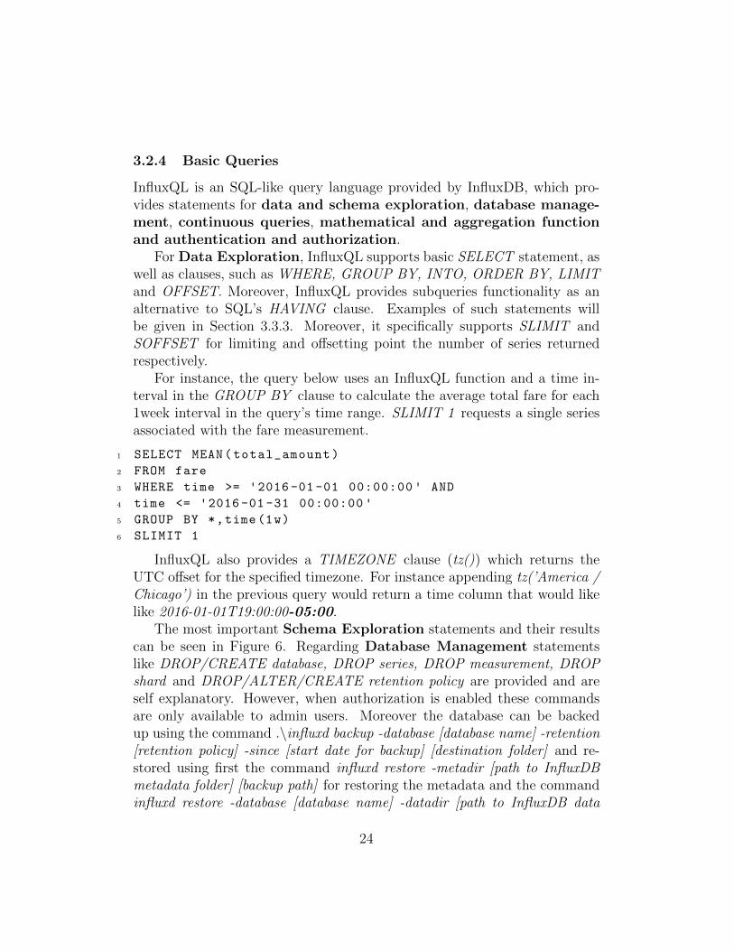
For instance, the query below uses an InfluxQL function and a time in-terval in the GROUP BY clause to calculate the average total fare for each1week interval in the query’s time range. SLIMIT 1 requests a single seriesassociated with the fare measurement.

1 SELECT MEAN(total_amount)

2 FROM fare

3 WHERE time >= '2016 -01 -01 00:00:00 ' AND

4 time <= '2016 -01 -31 00:00:00 '5 GROUP BY *,time(1w)

6 SLIMIT 1

InfluxQL also provides a TIMEZONE clause (tz()) which returns theUTC offset for the specified timezone. For instance appending tz(’America /Chicago’) in the previous query would return a time column that would likelike 2016-01-01T19:00:00-05:00.

The most important Schema Exploration statements and their resultscan be seen in Figure 6. Regarding Database Management statementslike DROP/CREATE database, DROP series, DROP measurement, DROPshard and DROP/ALTER/CREATE retention policy are provided and areself explanatory. However, when authorization is enabled these commandsare only available to admin users. Moreover the database can be backedup using the command .\influxd backup -database [database name] -retention[retention policy] -since [start date for backup] [destination folder] and re-stored using first the command influxd restore -metadir [path to InfluxDBmetadata folder] [backup path] for restoring the metadata and the commandinfluxd restore -database [database name] -datadir [path to InfluxDB data

24

Figure 6: Basic Schema Exploration statements.

folder] [backup path] for actually restoring the database.InfluxDB provides support for Continues Queries, namely queries that

run automatically and periodically on real-time data and store query resultsin a specified measurement. This is extremely important when it comes totime series and real time analysis for the reasons below14:

14InfluxData — Documentation — Continuous Queries. 2017. Retrieved from https:

//docs.influxdata.com/influxdb/v1.3/query_language/continuous_queries.

25

• Downsample Data. Use CQs to automatically downsample high pre-cision data to a lower precision and remove the high precision data fromthe database if not needed.

• Pre-calculate Expensive Queries.

• Substitute HAVING clauses and nested functions.

An example of such query can be seen below.

1 CREATE CONTINUOUS QUERY "cq_average_fare" ON "cabs"

2 RESAMPLE EVERY 30m

3 BEGIN

4 SELECT mean("total_fare")

5 INTO "average_fare"

6 FROM "fare"

7 GROUP BY time(1h)

8 END

cq average fare calculates the per hour average of total fare from the faremeasurement and stores the results in the average fare measurement in thecabs database.

cq average fare executes at 30-minute intervals (EVERY clause). Every30 minutes, cq average fare runs a single query that covers the time rangefor the current time bucket, that is, the one-hour time bucket that intersectswith current time (now()).

Finally InfluxDB provides various Functions and Operators, includ-ing, but not limited to, Aggregations e.g. MEAN, INTEGRAL, MODE,STANDARD DEVIATION, etc., Selectors e.g. PERCENTILE, SAMPLE(uses reservoir sampling), TOP, BOTTOM (Note that TOP and BOTTOMin InfluxDB is different than in SQL Server. They return the N greatest orlowest values for a specified field and not just the N latest or oldest ones.)Transformations e.g. HISTOGRAM, MOVING AVERAGE, DERIVA-TIVE and Predictors e.g. HOLT WINTERS method based on seasonality.

Since Holt Winters is quite unique in InfluxDB, it is worth mentioningthe structure of queries containing the method (the clauses in square bracketsare optional). There are two methods, HOLT WINTERS which returns onlythe predicted values, and HOLT WINTERS WITH-FIT, which returns boththe actual and predicted values. They both take as arguments the field thatshould be predicted, the number N of instances to be predicted and the

26

Figure 7: Identifying seasonality patterns for the sum of total fares in Chrono-graf. The dots represent the approximate seasonal data points. Each monthcontains 4 dots with similar pattern.

Figure 8: Executing the Holt Winters function in Chronograf.

27

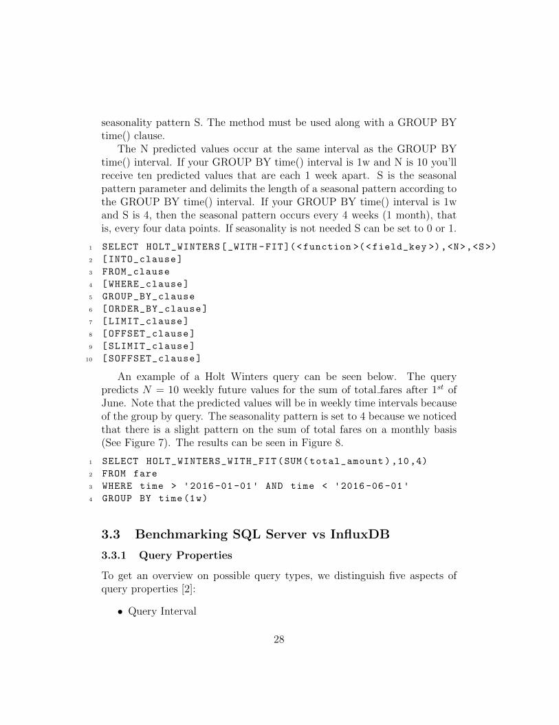
seasonality pattern S. The method must be used along with a GROUP BYtime() clause.

The N predicted values occur at the same interval as the GROUP BYtime() interval. If your GROUP BY time() interval is 1w and N is 10 you’llreceive ten predicted values that are each 1 week apart. S is the seasonalpattern parameter and delimits the length of a seasonal pattern according tothe GROUP BY time() interval. If your GROUP BY time() interval is 1wand S is 4, then the seasonal pattern occurs every 4 weeks (1 month), thatis, every four data points. If seasonality is not needed S can be set to 0 or 1.

1 SELECT HOLT_WINTERS[_WITH -FIT](<function >(<field_key >),<N>,<S>)

2 [INTO_clause]

3 FROM_clause

4 [WHERE_clause]

5 GROUP_BY_clause

6 [ORDER_BY_clause]

7 [LIMIT_clause]

8 [OFFSET_clause]

9 [SLIMIT_clause]

10 [SOFFSET_clause]

An example of a Holt Winters query can be seen below. The querypredicts N = 10 weekly future values for the sum of total fares after 1st ofJune. Note that the predicted values will be in weekly time intervals becauseof the group by query. The seasonality pattern is set to 4 because we noticedthat there is a slight pattern on the sum of total fares on a monthly basis(See Figure 7). The results can be seen in Figure 8.

1 SELECT HOLT_WINTERS_WITH_FIT(SUM(total_amount ),10,4)

2 FROM fare

3 WHERE time > '2016 -01 -01 ' AND time < '2016 -06 -01 '4 GROUP BY time(1w)

3.3 Benchmarking SQL Server vs InfluxDB

3.3.1 Query Properties

To get an overview on possible query types, we distinguish five aspects ofquery properties [2]:

• Query Interval

28

• Aggregation

• Object Identity

• Dimension

• Condition Type

However, some of these properties are not relevant to InfluxDB. Firstly,Dimension is not relevant since we are dealing solely with Time Dimension.InfluxDB is not a spatial Database. Also, Condition Type is not relevant,as InfluxDB supports only single object operations. According to InfluxDBdocumentation15 “Currently, there is no way to perform cross-measurementmath or grouping. All data must be under a single measurement to queryit together. InfluxDB is not a relational database and mapping data acrossmeasurements is not currently a recommended schema”.

As a result we exclude these properties from the queries below. Below,we present queries in InfluxQL that utilize combinations of the remainingproperties. The equivalent SQL queries are excluded from this reportbut can be found in the delivered project folder. In SQL a nonclustered index was created for the timestamp column to imitate InfluxDB’skey and improve SQL’s performance. When the index was removed, pointqueries on timestamp were up to 10 times slower. Note that point queriesutilizing time use precision in seconds in InfluxDB. Now, in our case suchpoint queries do not make sense but will be used for the sake of benchmarking.However, there might be cases where precision in seconds is actually relevant.

CLUSTERING IS A PREMIUM FEATURE IN INFLUXDB. THAT’SWHY WE COULD NOT TEST OUR QUERIES IN A CLUSTERED EN-VIRONMENT. ALL BENCHMARKING QUERIES WERE EXECUTEDIN A SINGLE NODE ENVIRONMENT.

3.3.2 Hardware Specifications

The benchmarking was executed using a Dell Inspiron 7559 laptop with thefollowing specifications:

• OS Name: Microsoft Windows 10 Home

15InfluxData — Documentation — Frequently Asked Questions. 2017. https://docs.influxdata.com/influxdb/v1.4/troubleshooting/frequently-asked-questions.

29

• System Type: x64-based PC

• Processor: Intel(R) Core(TM) i5-6300HQ CPU @ 2.30GHz, 2301Mhz, 4 Core(s), 4 Logical Processor(s)

• Installed Physical Memory (RAM): 16,0 GB

• L2 Cache Size: 1024 KB

• L3 Cache Size: 6144 KB

3.3.3 Benchmarking Queries

Query 1 (Range, Aggregation, Unknown): What was the total farecalculated per hour by the meters on New Year’s Day 2016?

1 SELECT SUM(fare_amount)

2 FROM fare

3 WHERE time >='2016 -01 -01 00:00:00 ' AND time <'2016 -01 -02 00:00:00 '4 GROUP BY time(1h)

Query 2 (Unbounded, Aggregation, Unknown): Which TPEP providerhas the maximum average trip distance for all recorder rides?

1 SELECT MAX(meanDistance),VendorID

2 FROM (

3 SELECT MEAN(trip_distance) AS meanDistance

4 FROM distance

5 WHERE time >='2016 -01 -01 00:00:00 '6 GROUP BY VendorID

7 )

Query 3 (Point, Aggregation, Unknown): How many passengershad payment disputes with drivers per TPEP provider for all recordedrides?

1 SELECT COUNT(passenger_count)

2 FROM passengers

3 WHERE payment_type='4'4 GROUP BY VendorID

30

Query 4 (Range, Aggregation, Known): What was the total farecalculated by the meters per day in January 2016 for CreativeMobile Technologies?

1 SELECT SUM(fare_amount)

2 FROM fare

3 WHERE time >='2016 -01 -01 ' AND time <'2016 -02 -01 ' AND VendorID='1'4 GROUP BY time(1d)

Query 5 (Unbounded, Aggregation, Known): How many passen-gers did VeriFone Inc. transport in total for all recorded rides perweek?

1 SELECT COUNT(passenger_count)

2 FROM passengers

3 WHERE time >='2016 -01 -01 ' AND VendorID='2'4 GROUP BY time(1w)

Query 6 (Point, Aggregation, Known): How many passengers trav-eled to JFK airport with VeriFone Inc. for all recorded rides?

1 SELECT COUNT(passenger_count)

2 FROM passengers

3 WHERE AND RatecodeID='2' AND VendorID='2'

Query 7 (Range, No Aggregation, Unknown): Which trip type(Rate Code) gave the company the highest single total fare amountin January 2016?

1 SELECT MAX(total_amount), RatecodeID

2 FROM fare

3 WHERE time >'2016 -01 -01 ' AND time <'2016 -02 -01 '

Query 8 (Unbounded, No Aggregation, Unknown): Which TPEPProvider covered the longest distance on a single ride since March2016?

1 SELECT MAX(trip_distance), VendorID

2 FROM distance

3 WHERE time >'2016 -03 -01 '

31

Query 9 (Point, No Aggregation, Unknown): We noticed that thereis an abnormally high fare value for timestamp 2016-03-10 22:59:51.Which TPEP provider charged a client with an abnormal fare andwhat is this fare?

1 SELECT VendorID , total_amount FROM fare

2 WHERE time = '2016 -03 -10 22:59:51 '

Query 10 (Range, No Aggregation, Known): Give the top-10 great-est tip amounts along with payment type for trips with John F.Kennedy International Airport as destination for spring 2016.

1 SELECT TOP(tip_amount ,10), payment_type

2 FROM fare

3 WHERE RatecodeID='2'4 AND time >='2016 -03 -01 ' AND time <'2016 -06 -01 '

Query 11 (Unbounded, No Aggregation, Known): Give the 10 low-est non-zero tips for individual rides with disputed fares since 2016.

1 SELECT BOTTOM(tip_amount ,10)

2 FROM fare

3 WHERE payment_type='4' AND tip_amount > 0

4 AND time >='2016 -01 -01 '

Query 12 (Point, No Aggregation, Known): Give exact fare amountand payment type for a ride starting at midnight on the 1st ofJanuary.

1 SELECT fare_amount , payment_type

2 FROM fare

3 WHERE time = '2016 -01 -01 00:00:00 '

3.3.4 Benchmarking Query Results

1. Write Performance: InfluxDB is designed to digest huge loads ofstreaming data (IoT, devOps, etc.) with the help of Kapacitor. How-ever, for our benchmarking we used historical data in CSV format.

32

Query Interval Aggregation Object Identity SQL Time InfluxDB Time

1 Range Yes Unknown 786 70

2 Unbounded Yes Unknown 3104.8 1537

3 Point Yes Unknown 621 33.2

4 Range Yes Known 2271.8 160.13

5 Unbounded Yes Known 2960 672.939

6 Point Yes Known 651.5 33.9

7 Range No Unknown 3079.1 1402.475

8 Unbounded No Unknown 2759.7 1584.96

9 Point No Unknown 4 2.5

10 Range No Known 663 628.14

11 Unbounded No Known 642.9 36

12 Point No Known 3.2 3

Table 3: Execution time in milliseconds (ms) for different query types in SQLServer and InfluxDB.

Figure 9: On-disk Compression: SQL Server vs InfluxDB.

33

InfluxDB does not have an official plugin that handles insertions fromCSV, thus an external tool was used as mentioned in Section 3.2.3.This tool converts CSV data to the appropriate format and then in-serts them to InfluxDB. However, SQL Server is designed to work withCSV data. Thus, the write throughputs cannot be comparable, as inInfluxDB we had to convert and then insert data, while in SQL Serverwe could import data immediately. That’s why we decided to excludewrite throughput from this report.

2. On-disc storage Requirements: For the same 30+ million rowsdataset, after writing all the values, the space consumed by the data setin case of SQL Server was 22.54 GB. However, InfluxDB only required0.83 GB. This results in approximately 692.3 bytes per record for SQLServer and 25.49 bytes per record for InfluxDB. For both databases thedefault configuration was used. See Figure 9 for a visualization of thiscomparison.

Conclusion: InfluxDB outperformed SQL Server in on-disk perfor-mance by 27x using default configuration.

3. Query Performance: Query performance was tested by using the 12benchmarking queries mentioned in Section 3.3.3 which cover 3 queryproperties (Query Interval, Aggregation and Object Identity) on a sin-gle node. Each query was executed 11 times and its average executiontime was calculated excluding the first execution. It was found thatthe average of all query responses for SQL Server was 1462.25 ms andfor InfluxDB was 513.68 ms (See Figure 11). The individual averageexecution times per query can be seen in Table 3 and Figure 10. Wenotice that for queries 9 and 12 InfluxDB has similar performance toSQL Server. These are point queries on the timestamp and the SQLdatabase has an index built on the timestamp. If this index is re-moved its performance decreases 10x. Furthermore, query 10 for whichInfluxDB and SQL Server perform similarly uses function TOP of In-fluxDB. We noticed that this function is slower than the respectiveBOTTOM one. This behavior based on common sense is not rationaland could be the result of a bug. Other than these 3 queries, for theremaining 9 queries InfluxDB outperforms SQL Server.

Conclusion: InfluxDB is up to 20x faster than SQL Server in queryperformance with an average of 8x faster. Note that since InfluxDB’s

34

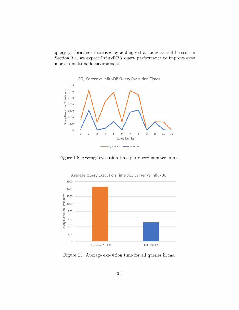
query performance increases by adding extra nodes as will be seen inSection 3.4, we expect InfluxDB’s query performance to improve evenmore in multi-node environments.

Figure 10: Average execution time per query number in ms.

Figure 11: Average execution time for all queries in ms.

35

3.4 Benchmarking

This section will compare performance of 3 commonly used technologies fortime-series data: Cassandra, OpenTSDB and Elasticsearch with InfluxDB.See Figure 5 to see the comparison of some basic features of these technolo-gies. Please note that all the content and statistics used in thissection are from the official benchmarking by influxDB [3]. Thefollowing paragraphs introduce the metrics and data set against which thisbenchmarking is done.

Metrics: The benchmarking is done against the most commonly evalu-ated characteristics for working with time-series data which are:

1. Data ingest performance - measured in values per second.

2. On-disk storage requirements - measured in Gigabytes.

3. Mean query response time - measured in milliseconds.

The Data Set: The dataset used for these benchmarks, models a com-mon DevOps monitoring and metrics use case, where a number of serversare periodically reporting system and application metrics at a regular timeinterval. Overview of the data can be seen in Table 4.

Parameters Cassandra OpenTSDB Elasticsearch

Number of Servers 1000 1000 100

Values measuredper Server

100 100 100

MeasurementInterval

10s 10s 10s

Dataset dura-tion(s)

24h 4h 24h, 48h, 72h, 96h

Total values indataset

864,000,000 per day 144,000,000 864,000,000 per day

Table 4: Overview of the Parameters for the Sample Dataset.

3.4.1 InfluxDB vs. Cassandra

Let us compare the performance of InfluxDB and Cassandra with respect tothe the 3 above mentioned vectors [5].

36

1. Write Performance: To test write performance, batch of 24-hourdataset with 4 worker threads was concurrently loaded (to match thenumber of cores on the server). The average throughput of Cassandrawas found to be 90,333 values per second .The same dataset loadedinto InuxDB at a rate of 476,460 values per second (See Figure 12).

Figure 12: Write Performance: InfluxDB Vs. Cassandra

Conclusion: InuxDB performed better than Cassandra by 5.3x whencomparing data ingestion performance.

2. On-disk storage Requirments: For the same 24-hour dataset, afterwriting all the values the space consumed by the data set in case ofCassandra was 13.0 GB however influxDB only required 1.4 GB. Thisresults in approximately 1.77 bytes per value for InuxDB and 16.15bytes per value for Cassandra. See Figure 13 for detailed view.

Conclusion: According to this benchmark, InfluxDB outperformedCassandra by 9.3x better on-disk compression.

3. Query Performance: To test query performance an aggregation querywas chosen that aggregates data for a single server (single time series)over a random 1-hour period of time, grouped into one-minute inter-vals, potentially representing a single line on a visualization - a commonDevOps monitoring and metrics function. It is a very common use casefor IoT. Cassandra has 2 scenarios, one where all of the query process-ing is handled on the client side, and another where Cassandra was

37

Figure 13: On-disk Compression: InfluxDB Vs. Cassandra

asked to return results for a set of queries, which forced all of the queryprocessing to happen on the server side. Figure 14 shows that Cassan-dra was only able to deliver performance comparable to InfluxDB inthe scenario where the application handled the query load. However,InfluxDB outperformed Cassandra by being x20 times faster than itwhen processing happened on the server side. And if we increase timeperiod to 12 hours or if we increase number of time series, that is queryover multiple servers, Cassandra is even slower and in such scenarioseven if all the query load is handled by client side, Cassandra is waybehind than InfluxDB.

Conclusion: InfluxDB is upto 168x faster than Cassandra in queryperformance (server side aggregations) [5].

3.4.2 InfluxDB vs. Elasticsearch

The statistics of benchmarking of InfluxDB against Elasticsearch are takenfrom the technical benchmarking report from official influx data benchmark-ing [6].

1. Write Performance: For testing of write performance, 24h datasetwith 4 worker threads (to match the number of cores on the server)were loaded. The average throughput of Elasticsearch was found to be115,422 values per second, however InfluxDB loaded the same data at

38

Figure 14: Query Performance: InfluxDB Vs. Cassandra

a rate of 926,389 values per second. The write throughput remainedalmost constant with larger data sets (48h, 72h and 96h).

Figure 15: Write Throughput: InfluxDB Vs. Elasticsearch

Conclusion: InfluxDB was proven to be 8 times better than Elastic-search in write performance (See Figure 15).

2. On-disk storage Requirments: To test on-disk compression the

39

benchmarking is done both against recommended configuration for timeseries data and default configuration of Elasticsearch. For 24 hourdata-set the amount of space utilized by InfluxDB was 127 MB, how-ever Elastic search required 2.1 GB with default settings and 502 MBwith the recommended configurations. So approximately space neededfor InfluxDB was 1.54 bytes per value and 6.09 bytes per value forElasticsearch. Figure 16 shows this comparison in form of bar chart.

Figure 16: On-disk Compression: InfluxDB Vs. Elasticsearch

Conclusion: InfluxDB outperformed Elasticsearch in on-disk com-pression by 4x and 16x in recommended and default configuration re-spectively.

3. Query Performance: Query performance was tested by aggregatingvalue on random 1-hour period of time, grouped into one-minute in-tervals, representing a single line on a visualization (Querying singletime series is a common use case for DevOps and IoT). It was foundthat the mean query response time for Elasticsearch was 4.98ms (201queries/sec) and for InfluxDB was 1.26ms (794 queries/sec) for thesame query, which shows that InfluxDB was 4x faster in this case. Itcan be seen in Figure 17 that as size of the dataset increases perfor-mance of Elasticsearch degrades while the performance of InfluxDBremain constant.

Conclusion: InfluxDB outperformed Elasticsearch by proving to be

40

Figure 17: Query Performance: InfluxDB Vs. Elasticsearch

4x to 10x better query performance depending on how large is thedata-set.

3.4.3 InfluxDB vs. OpenTSDB

To compare InfluxDB with OpenTSDB, the benchmarking done in this sec-tion is taken from the technical benchmarking report from official influx databenchmarking [7].

1. Write Performance: For testing of write performance, 24h datasetwith 4 worker threads (to match the number of cores on the server)were loaded. In addition to that, because target OpenTSDB setuprequired 6 servers in total (4 HBase nodes + 2 OpenTSDB daemons,and exclusive of the additional Zookeeper node) compared to just asingle InfluxDB node, so write performance was looked at per serverbasis. Additionally, replication factor of 1 with in H-base is used tomake a fair comparison with a single node of InfluxDB. The averagethroughput of OpenTSDB was found to be 35,648 values per second(per server). Data ingestion for InfluxDB was at a rate of 179,814 valuesper second (per server) for the same database. per-server throughput.

Conclusion: InfluxDB outperformed OpenTSDB by 5.0x when eval-

41

Figure 18: Write Throughput: InfluxDB Vs. OpenTSDB

uating write throughput.

2. On-disk storage Requirments: For the data mentioned above, theamount of disk space consumed by OpenTSDB was 5.8 GB. The samedataset required only 351MB for InfluxDB. This results in approxi-mately 2.44 bytes per value for InfluxDB and 40.3 bytes per value forOpenTSDB.

Figure 19: On-disk Compression: InfluxDB Vs. OpenTSDB

Conclusion: InfluxDB outperformed OpenTSDB by 16.5x when eval-

42

uating on-disk compression.

3. Query Performance: To test query performance, the query selectedis the one that aggregates data for 8 servers over a random 1-hour pe-riod of time, grouped into one-minute intervals, potentially representingmultiple lines on a visualization which is a common DevOps monitor-ing and metrics function. Concurrency was increased in the queries,starting from 1 worker upto 32 workers to check how each databaseperform in the situation of increasing work load. It can be see fromFigure 20, InfluxDB performed better than OpenTSDB in all scenariosand there was only a slight variance across different concurrencies. Ifwe see the architecture of OpenTSDB, these results are logical becausein OpenTSDB each query has to reach out to H-base to retrieve databefore performing query which adds to latency and hence results inslower response time.

Figure 20: Query Performance: InfluxDB Vs. OpenTSDB

Conclusion: InfluxDB was proven to be 4.0x faster than OpenTSDBin query performance.

43

References

[1] DB-Engines. Db-engines ranking, 2017.

[2] Duntgen, C., Behr, T., and Guting, R. H. Berlinmod: A bench-mark for moving object databases. The VLDB Journal 18, 6 (Dec. 2009),1335–1368.

[3] InfluxData. Influxdb version 1.3 documentation, 2017.

[4] Joshi, P., Massaron, L., and Hearty, J. Python: Real WorldMachine Learning. Packt Publishing, 2017.

[5] Persen, T., and Winslow, R. Influx db vs. cassandra for time-seriesdata, metrics & management. Tech. rep., September 2016.

[6] Persen, T., and Winslow, R. Influx db vs. elasticsearch for time-series data, metrics & management. Tech. rep., September 2016.

[7] Persen, T., and Winslow, R. Influx db vs. opentsdb for time-seriesdata, metrics & management. Tech. rep., November 2016.

44