time use, computable general equilibrium and tax … · 2005-02-14 · 1 time use, computable...
TRANSCRIPT
1
TIME USE, COMPUTABLE GENERAL EQUILIBRIUM
AND TAX POLICY ANALYSIS
Javier Ferri (1)
María Luisa Moltó (1)
Ezequiel Uriel (1)(2)
(This version February 2005,
comments are welcome)
(1) University of Valencia
(2) Instituto Valenciano de Investigaciones Económicas (Valencian Institute of
Economic Research)
2
Abstract
The motivation behind this paper is to provide some guidance on how to apply a general
equilibrium model with home production in a real world setting to analyze economy-wide tax
policies. The story line is the model of Iorweth and Whalley (2002) that we write as a mixed
complementarity problem to make it ready to easily accommodate more consumers, commodities
and household production functions. The model evaluates the welfare impact of introducing the
VAT on food in a context in which households can produce home meals for own consumption
that compete with meals served in restaurants. With this model at hand we proceed as follows:
firstly, we replicate some of the IW results and confirm that they depend on the elasticity of
substitution between food and time in the household production of meals. Secondly, we move to
the Spanish data and simulate the effects on welfare of different fiscal experiments. Finally, we
enlarge the number of consumers and tackle some distributional issues.
3
1. Introduction
Simulation models have been extensively used over the last decades to analyze the effects
of economy-wide tax policies. Two approaches can be distinguished: micro-simulation
models within a partial equilibrium framework (see Bourguignon and Spadaro, 2005, for a
discussion) and large scale computable general equilibrium (CGE) models within a general
equilibrium framework (see Fullerton and Metcalf, 2002, and Shoven and Whalley, 1992).
This paper focus in the second approach. In a typical CGE exercise, many firms and
households are characterized by means of a set of equations embodying optimal behaviour
and their interaction determines prices and quantities that are or would be observed in the
market. Most of the times, in this exercise, the role of the households is reduced to provide
factors for market production and purchase goods and services in the market. However,
households play an important role in the economies not only as consumers but also as
producers, although only a small part of that production goes through the market whereas
a substantial amount (mainly services) is produced and consumed within the home.
The idea of households behaving as enterprises using time, services of capital and
intermediate inputs to produce commodities for own consumption go back to Becker
(1965) and Gronau (1977) and has influenced different areas of economic analysis (see
Gronau, 1997 for a survey on the relevance of household production theory in labor
economics). In public finance, an accurate measure of the household production in the
economic structure is basic for tax policy analysis. Thus, the welfare impact of different
taxes depends on how different households combine unpaid work, capital and intermediate
goods to produce goods and services ready to be consumed. The empirical importance of
household production for the theory of optimum tax policy has been discussed in previous
studies, as those of Boskin (1975), Sandmo (1990) or more recently Kleven et al (2000),
Anderberg and Balestrino (2000) and Kleven (2004), whereas numerical simulations
quantifying the effects have been exploited by Piggott and Whalley (1996); Piggott and
Whalley, (2001) and Iorwerth and Whalley (2002).
However, the bulk of the existing empirical literature that integrates taxes and household
production focus on pure efficiency aspects and a representative consumer, sidestepping
distributional issues, or reducing them to the bare minimum; e.g Piggott and Whalley
(1996) -households with and without children-; Anderberg and Balestrino (2000)– low
4
ability and high ability- and Piggott and Whalley (2001) -rich and poor-. Despite the
relevance of simulation models as a powerful tool for the analysis of public policies and the
important dimension of household production, no previous attempt has been done to tie
self supply to CGE models in order to quantify the economy-wide effects of tax policy.
This paper aims to bridge this gap, by illustrating the way in which CGE techniques can be
applied to models in which the household production is a key variable.
In the carrying out we go from an efficiency to an incidence analysis of tax policy, but for
illustrative purposes we maintain the model as stylized as possible. The story line is the
model of Iorweth and Whalley (2002) – IW henceforth – that we write as a mixed
complementarity problem because it makes the model suitable to easily accommodate more
consumers, commodities and household production functions. This model evaluates the
welfare impact of introducing the VAT on food in a context in which households can
produce home meals for own consumption. With the model in a mixed complementarity
format at hand we pursue three objectives. Firstly, we replicate some of the IW results as a
checkpoint. IW show that extending the sales tax to cover food leads to welfare gains in its
model and that an optimal tax scheme involves a higher tax on food than on other goods.
With one input good and one consumption good, Anderberg and Balestrino (2000)
demonstrate that the input good should be taxed at a higher rate than general consumption
if the degree of complementarity in household production is larger than the degree of
complementarity in consumption. We confirm that the more general IW results also
depend on the elasticity of substitution between food and time in the household
production of meals, coming to be the opposite when the elasticity is high enough.
Secondly, we move to the Spanish data and simulate the effects on welfare of different
fiscal experiments, maintaining the assumption of a representative consumer. The standard
approach in applying large scale general equilibrium models (Shoven and Whalley, 1992)
typically requires a set of equations calibrated with respect to a “reality” represented as a
benchmark database called social accounting matrix (SAM). Thus, the calibration of a CGE
model including household production would need a social accounting matrix extended to
consider, in addition to the market economy, the production of services provided by
households through unpaid work. Matching standard information from input-output tables
and consumer expenditure survey, among other, with time use surveys, Uriel et al. (2005)
elaborate a social accounting matrix that for the first time implements the conceptual
framework sketched by Pyatt (1990). This extended social accounting matrix (ESAM)
5
integrates the portion of household production currently outside the boundaries of the
SNA, into the market flows of a more conventional social accounting matrix. This paper
makes use of an abridge version of the ESAM to calibrate the model for the Spanish
economy. The results on aggregate welfare for Spain are consistent with those obtained for
Canada.
Finally, we enlarge the number of consumers to three groups and tackle a differential tax
incidence analysis for the Spanish economy. The theory of taxation deals with the problem
of levy taxes to enhance economic efficiency and to contribute to a fair distribution of
resources. At this point we explore up to which extend the government can improve
welfare by enhancing both efficiency and fairness. In some sense, this last exercise can be
considered as a first approximation towards a more elaborated CGE model with all the
main ingredients considered here – taxes, household production, efficiency and equity.
Thus, the extension to a fully represented economy, such as the one described in the
ESAM is, to a great extent, a matter of scale.
In section 2 the motivation of the illustrative fiscal experiment is set; the model’s equations
are presented in section 3; section 4 introduces the data used for calibrating the models. In
section 5 the results of the different tax policy experiments are offered, including the
replication of IW experiments, efficiency and optimal taxation for in Spain and some tax
incidence considerations. Finally, Section 6 summarises the paper and suggests future
follow-ups to this line of research.
2. The VAT on food and restaurants in Spain and the importance of
household production
The VAT in Spain was introduced in 1986 but the legislation has suffered several
modifications since then, the last big reform taking place in 1995. As a consequence, at the
present the VAT is levied at three rates in Spain: a general rate of 16%, a low rate of 7%
(that affects, among others, to restaurants) and a very low rate of 4% (that affects, among
others, to some kinds of food). Since the sixth directive in 1977 certain steps have been
taken towards harmonising value added tax in the European Union so that the future
legislation in the member states related to VAT should be conform with the different
directives of the European institutions. In 1996, the European Commission proposed a
programme to establish a definitive VAT system. In 2001, a Commission report provided
6
the possible guidelines to be followed in the medium term for the harmonisation of
reduced VAT rates. The proposal consists in establishing a minimum general rate of 15%
and two reduced VAT rates to be applied to a set list of goods and services: one reduced
rate around the 5% mark and another super-reduced rate that is not specified, for those
goods and services which, for historical or economic reasons, require differential treatment.
Restaurants did not appear in either list, although food was included. However, in 2003, a
proposal of directive include restaurants in list H, allowing to member states the
implementation of a reduced rate to restaurant services.
The illustrative example in this paper focuses on efficiency as well as equity considerations
related to possible changes in VAT rates applied to restaurants and food. The model
considers both the market production of meals by restaurants, as well as the preparation of
food at home. The restaurant production -the meals served there- compete directly with
the meals produced by households themselves, the VAT the latter pay on food being a
significant part of production costs. Both households and restaurants use labour and food
to produce meals, but the fiscal treatment of the two types of production is very different.
In the first place, restaurants can deduce the VAT levied on the food they purchase, while
the household production of meals, as it is not a market activity, must bear the full amount
of VAT that is levied on food. In the second place, restaurants must include VAT in their
invoices for the service offered, whereas the meals produced by households are exempt.
Finally, households must pay a part of the revenue generated, in the form of income tax,
through dedicating part of their available time to market activities. There are, therefore, two
sources of distortion in the fiscal treatment of the production of meals that generate
inefficiency. One type of distortion refers to the different fiscal treatment of goods of very
similar characteristics: homemade meals and those produced by restaurants. Another
distortion is due to the inputs required for the production of homemade meals (labour and
food) receiving different fiscal consideration.
Under the equal yield premise by making food exempt from VAT, the distortion between
inputs used in household production is eliminated, but the distortion between market and
household production is widened. A decrease in the VAT charged by restaurants, on the
other hand, reduces the distortion between market and non-market goods, but widens the
gap between the fiscal treatment of food and labour in household production of meals. In
both cases, the theoretical effect on efficiency is ambiguous. IW simulations nevertheless
suggest that an increase in VAT on food and a reduction in VAT on restaurants would
7
improve the efficiency of the current tax system and would lead to gains in global well-
being. As we show below, these results are very conditional to the elasticity of substitution
between food and time in the household production of meals.
Generally speaking, an increase in the VAT levied on food and a reduction in the VAT
applied to restaurants could have adverse effects in terms of redistribution, as those
households that are economically most disadvantaged would be penalized, due to the fact
that they have more meals at home than in restaurants. By writing the equations as a mixed
complementarity problem, as in this paper, extending the demand side of the model to deal
with the economic incidence of a tax is an issue that depends on the information contained
in the extended social accounting matrix. Further, in this paper, we divide the consumers in
three groups according to their income level.
3. The model
3.1 A simple model with household production
To provide an intuition of how household production can be incorporated in a general
equilibrium framework let us first borrow the specific model structure of Kleven et al.
(2000). In this model there exist three categories of goods. The first category consists of all
goods and services provided exclusively by the market (referred to as “market goods” from
now onwards), which will take the letter M. The second group is made up of services that
can be produced by both the market and also the household. Home production of meals
and the elaboration of meals in restaurants were chosen from among all of these products,
in accordance with our objective1. The goods that are included in this category will be
denoted by S and the meals produced by restaurants and in the household will be
distinguished by the letters R and H. Finally, a representative consumer can also obtain
utility from leisure L0. Let assume at this stage that the utility function is weakly separable
in three blocks and that the labour time is the only relevant input for production. Let LH be
the time devoted to household production, LN = LM+LR the time used for market
production (M and R) and L the total labour endowment. Self-supplied services are
1 There are other examples, such as caring for children or old people, the production of clothing and accommodation that are not considered in this analysis.
8
produced by means of a household production function R=R(LH). The representative
consumer has a utility function defined over those goods exclusively produced by the
market (M) meals - S(R, H) - and leisure (L0), and thus we can write the model as a non-
linear programming problem in the following way:
0max ( , ( , ), )U U M S R H L=
s.t.
(0.1) ( )MM M L=
(0.2) ( )RR R L=
(0.3) ( )HH H L=
(0.4) 0 H NL L L L= − −
(0.5) N M RL L L= +
(0.6) L N M RP L P M P R= +
Note that using (0.4), substituting for NL into (0.6) and adding ( )H HP H L to each side of
the equation the budget constraint may be rewritten as:
(0.7) 0M R H L L H L HP M P R P H P L P L P H P L+ + + = + −
where P with a subscript represents a price, PR standing for the shadow price of domestic
production. Thus, this problem defines an utility function over a set of goods and services,
including self-supplied services, and a budget constraint in which total income is given by
the value of the total endowment of time augmented by the shadow profits derived from
the household production activity. The consumers take that income and ''buy'' goods and
services provided by the market and services produced at home.
9
An important feature of expression (0.7) is that in order to define the competitive
equilibrium we need to add to the system of equations an additional activity H acting in the
same way as the other but whose profits flow directly to the consumer income. As Sandmo
(1990) wrote “is in fact as if a household production department maximized household
profit”.
The previous simple model can be extended in the same way as Iorweth and Whalley
(2002). Thus, we can add a new good “food” (A) which can be considered an input
exchanged in the market, used together with labour in the production of R (LR, AR) and H
(LH, AH). Additionally, the representative consumer has a set quantity of total resources,
G*, which he or she can convert into food, A, or into units of effective labour, L, by
means of a transformation frontier. With these changes the previous model can be
rewritten in the Iorweth and Whalley form as:
0max ( , ( , ), )U U M S R H L=
(0.8) 0 H M RL L L L L= − − −
(0.9) ( )MM M L=
(0.10) ( , )R RR R L A=
(0.11) ( , )H HH H L A=
(0.12) ( ),G G L A=
(0.13) H RA A A= +
(0.14) ( )0M R H L L A H L H A HP M P R P H P L P L P A P H P L P A+ + + = + + − −
Where (0.12) represents the transformation frontier by means of which total resources G
yields different combinations of labor and food. The right hand side of the expression
(0.14) is the total income (including any profit from the household activity) whereas the left
hand side reflects the use of the income.

10
3.2 The household production model as a mixed complementarity problem
In this subsection we write the household production model as a mixed complementarity
problem (MCP) taking into account the different taxes considered in the simulations.
Mathiesen (1985) demonstrated that an Arrow-Debreu type general equilibrium model
could be efficiently formulated and solved through a mixed complementarity problem with
three categories of variables: (a) a non-negative vector of commodities prices, including
final goods, intermediate goods and production factors; (b) a non-negative vector of
activity levels for the sectors that use technologies of constant returns of scale; and (c) a
vector of income levels for each type of “institution” in the model, including households
and the government.
Equilibrium in these three categories should satisfy a system that responds to the optimal
behaviour of economic agents, with three classes of nonlinear inequalities. These
inequalities indicate that: (a) the level of activity in each productive process implies the
condition of zero profit; (b) the market for each commodity is cleared; and (c) consumer
income coincides with the revenue generated by his or her available resources. The solution
to this problem is the general equilibrium of the economy.
What follows is a presentation of the model used in the simulations as a mixed
complementarity problem, which first tackles consumer and producer optimisation
problems that give rise to cost and expenditure functions. As far as restaurant and
household meals are concerned, we will assume that technology is represented by a
production function with constant elasticity of substitution (CES). Producers minimise
costs for a certain volume of output, obtaining the conditional factor demand and the
corresponding cost function. For example, restaurants will solve the following optimisation
problem:
Min APLP AL +
s.a ( ) ( ) ( )[ ] ( )1//1/1 1−−− −+= RRRRRR ALR RRR
σσσσσσ δδφ
where Rσ is the elasticity of substitution between labour and food in restaurants’ meals
production technology. The demand functions conditioned to R are:
11
(0.15) ( ) ( )
( )
RP
PL
RRR
LR
ARRRRR
σσσ
δδ
δδφ
−−−
−
−+=
1/11
11
(0.16) ( ) ( )( )
RP
PA
RRR
RAR
LRRRR
σσσδ
δδ
δφ
−−−
−+
−=
1/11 1
1
If 1=R and factor demand is replaced in the objective function in the above optimisation
problem, the cost function for restaurants per unit of output is obtained:
(0.17) ( ) ( )
( )RRR
R
A
R
LRALR
PPPPC
σσσ
δδφ
−−−−
−
+
=
1/1111
1,
Shephard’s lemma affirms that the derivative of the previous cost function with respect to
the price is the quantity of factor demanded per unit of output. In particular:
(0.18) ( )R
LP
PPC R
L
ALR =∂
∂ ,
(0.19) ( )R
AP
PPC R
A
ALR =∂
∂ ,
The cost function for household production of meals can be defined in the same way
( )ALH PPC , from which we can obtain the optimal quantity of food and labour
employed in preparing meals at home. However, we must now consider the VAT on food,
which raises the purchasing price of food for home production of meals, so the quantities
LH and AH will differ from those obtained when the tax is not applied.
(0.20) ( )( ), 1H L A A H
L
C P P IVA LP H
∂ +=
∂
(0.21) ( )( )
( )( ), 11
H L A A H
A A
C P P IVA AHP IVA
∂ +=
∂ +
Moreover, we will assume that market goods are produced solely by means of labour
)( MLMM = , resulting in producers minimising factor costs (in this case, only labour)
12
subject to a production function that only depends on labour. If furthermore, constant
returns to scale are assumed to exist, the problem of minimising costs for “market good”
producers would be expressed as:
Min LPL
s.a LM =
from where the trivial unit cost function LLMM PPCC == )( is obtained and, therefore:
(10) ( )
1==∂
∂M
LP
PC M
L
LM
There is also a fictitious sector that uses those goods consumed by households as inputs
and produces “welfare” as output. In the MCP approach, this sector is nothing more than
the utility function of the representative household whose arguments are the consumption
of “market goods”, meals and leisure. Meals can be both homemade and from restaurants,
and these two inputs are not necessarily perfect substitutes. The utility function of a
household is therefore expressed as:
(0.22) ( )( ), , , oU M S R H L
separability is taken into account in preferences, insofar as the consumer firstly chooses
between leisure or consuming goods and services. A second choice would be between
consuming “market goods” and meals. Finally, the consumer chooses optimal
consumption of restaurant meals and homemade meals. Let PS be the price of the
composite basket of meals produced in restaurants and inside the home, and let PB be the
price of the composite basket of “market goods” and meals2. The unit cost function for
this “welfare” sector is what the literature calls expenditure function, and it provides the
minimum necessary cost, given the price of the goods, to obtain a unit of utility or welfare:
2 PS is a function of PR and PH whereas PB is a function of PS and PM.
13
(0.23) ( ),oU U L BC C P P=
where:
(0.24) ( )( )1 ,B B B M M SP C C P IVA P= = +
and:
(0.25) ( )( )1 ,S S S R R HP C C P IVA P= = +
with IVAM representing the average VAT rate applied to “market goods” and IVAR the tax
on value added charged by restaurants. As seen above, all the cost functions are derived
from a optimisation problem assuming CES functions for the technology.
In our approximation an additional activity is introduced called TL which transforms
leisure (whose price is given by oLP ) into labour supply, at a price of LP : )( oLTLTL = .
This artifice enables us to identify the reaction of labour supply in the different
experiments. The cost function of this activity is represented by:
(0.26) (1 ) ( )o oL TL L LP TING C P P− = =
Therefore, the deviation between the value of leisure and the market wage is caused by the
tax levied on income derived from labour (TING). Note that IVA is a tax-exclusive rate,
that is, the rate is expressed as a fraction of the price excluding tax, whereas TING is a tax-
inclusive rate.
By applying the Shephard’s lemma to expressions (0.23), (0.24) and (0.25) we obtain the
amount of leisure, “market goods” and meals demanded by the representative consumer:
(0.27) ( ),
o
o
U L B o
L
C P P LP U
∂=
∂
(0.28) ( )( )( )( )1 ,1
B M M S
M M
C P IVA P MBP IVA
∂ +=
∂ +
(0.29) ( )( )( )( )1 ,1
S R R H
R R
C P IVA P RSP IVA
∂ +=
∂ +
14
(0.30) ( ),S R H
H
C P P HP S
∂=
∂
The representative household transforms total available resources G into a composite
basket V of food and labour (that may or may not be offered to the market) by means of
the trivial production function ( )V V G= meaning that:
(0.31) ( )V G GC P P=
At the same time, V transforms resource units into food or units of effective labour,
following a constant elasticity of transformation (CET) function.
(0.32) 1 1 1
(1 )G L A
εε ε εε εξ τ τ+ + +
= + −
wherebyε is the transformation elasticity. The household maximises income P L P ALo A+
in light of condition (0.32). This function is concave both in L and A and this allows us to
obtain an upward sloping supply curve for food and for units of effective labour. The price
of the composite good can be obtained by a nonlinear combination of OLP and PA:
( )1/(1 )1 1 1(1 )OV L AP P P
εε ε ε εξ τ τ+− − + − += + −
Once the cost functions that incorporate agents’ optimising behaviour are established, the
mixed complementarity problem, whose solution guarantees the existence of overall
equilibrium in the economy, can be written in the following way:
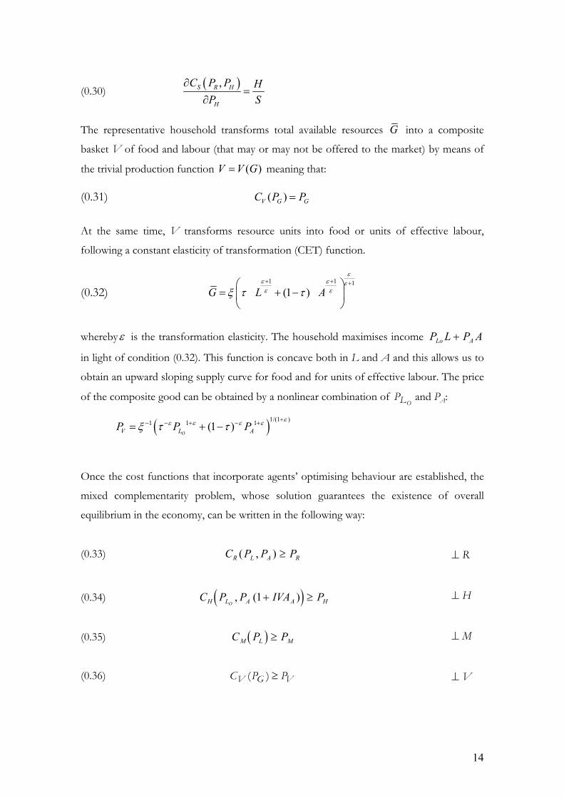
(0.33) C P P PR L A R( , ) ≥ ⊥ R
(0.34) ( )C P P IVA PH L A A HO, ( )1+ ≥ ⊥ H
(0.35) ( )C P PM L M≥ ⊥ M
(0.36) VGV PPC ≥)( ⊥ V
15
(0.37) ( )C P P PU L B Uo, ≥ ⊥ U
(0.38) C P P TINGTL L LO( ) ( )≥ −1 ⊥ TL
(0.39) ( )( )
(1 ),(1 )
B M M S
M M
C P IVA PM B
P IVA∂
∂+
≥+
⊥ PM
(0.40) ( )( )
(1 ),(1 )
S R R H
R R
C P IVA PR S
P IVA∂
∂+
≥+
⊥ PR
(0.41) ( )( )
(1 ),(1 )
S R R H
H R
C P IVA PH S
P IVA∂
∂+
≥+
⊥ PH
(0.42) ( ) ( )
( ), , (1 )( )
(1 )O OO
O O O
U L B H L A ATL L
L L L A
C P P C P P IVAC PL TL U H
P P P IVA
∂ ∂∂∂ ∂ ∂
+≥ + +
+
⊥ PLO
(0.43) ( ) ( )
TLC P P
PR
C PP
MR L A
L
M L
L
≥ +∂
∂∂∂
,
⊥ PL
(0.44) ( )( )
( )( )( ), 1 ,
1OH L A A R L A
AA A
C P P IVA C P PA
PP IVA
∂ + ∂≥ +
∂∂ +
⊥ PA
(0.45) UPIU /≥ ⊥ PU
(0.46) ( )V G
G
C PGP
∂≥
∂
⊥ PG
(0.47) G A A R R M M LI P G IVA P H IVA P R IVA P M TING P TL= + + + +
⊥ I
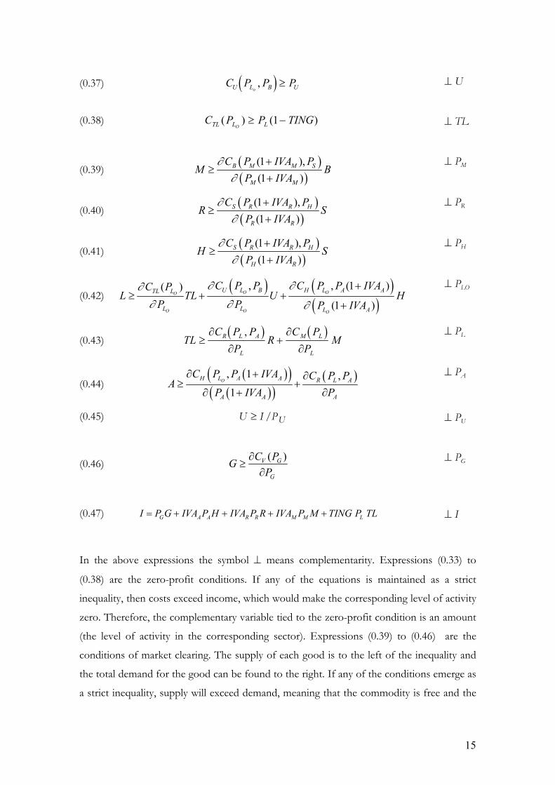
In the above expressions the symbol ⊥ means complementarity. Expressions (0.33) to
(0.38) are the zero-profit conditions. If any of the equations is maintained as a strict
inequality, then costs exceed income, which would make the corresponding level of activity
zero. Therefore, the complementary variable tied to the zero-profit condition is an amount
(the level of activity in the corresponding sector). Expressions (0.39) to (0.46) are the
conditions of market clearing. The supply of each good is to the left of the inequality and
the total demand for the good can be found to the right. If any of the conditions emerge as
a strict inequality, supply will exceed demand, meaning that the commodity is free and the
16
price will be zero. Therefore, the complementary variable in conditions of market clearing
is the price of the corresponding commodity. The last expression (0.47) captures the
revenue equilibrium condition. The representative consumer’s total income (I) is the sum
of the market value of total resource endowment plus revenue obtained by collecting
different taxes. It is important to note that although the dimension of the problem would
be different, the structure of the equations remains the same in a model with more
activities, factors and households.
3. The data
The starting point for calbrating a general equilibrium model should be a
microeconomically consistent data set, which in reality means that it is consistent with the
mixed complementarity problem specified in the previous section. Therefore, our data base
for calibration must satisfy the condition of zero profit, market clearing and income
equilibrium.
The consideration of household production of meals is a focal point of our study. The
estimate of time spent on preparing meals at home, as well as the food inputs used in this
production is information that is available in the extended social accounting matrix
(ESAM-95) for the Spanish economy in 1995. The core of the market side of this data set
is the last available Input-Output Framework (IOF-95) of National Accounts for Spain.
However, in order to establish the correspondence between the income of factors and the
different types of households, information from the European household panel survey
(ECHP) has been used Finally, whereas the distribution of consumption by household type
is obtained from the Household Expenditure Survey. To estimate the working time at
home we use data from a survey on the use of time provided by the Spanish Women’s
Institute (see Uriel et al, 2005, for more details).
The complete matrix distinguish ten groups of economic activities and four types of
household production functions. Both, household activities and market activities use labor,
capital and a complete set of intermediate inputs to produce. The labor factor, in turn, is
disaggregated according to educational level and gender (both, at the household and at the
market level), and the households are classified by level of income. The classification for
labor, together with the detail for households offers a rich representation of the
distribution of the full income in the economy. This information, nevertheless, requires
17
some adjustments to adapt it to the simplified model presented in this paper. The resulting
data set, when no detail in the home account is carried out, can be consulted in Table 1,
which is a very abridged form of a SAM that we have entitled “Basic Social Accounting
Matrix 1995”. This matrix captures the income flows that interest us in a standard way in
accordance with the SAM notation.
{Insert Table 1}
The rows represent “income” and the columns “expenditure”. For example, the first
column ventures that Spanish households spent more than six trillion pesetas in restaurants
and prepared meals at home worth 18 trillion. Leisure worth more than 125 trillion pesetas
was also consumed. Furthermore, nearly seven trillion pesetas worth of food and almost 12
trillion pesetas worth of household labour were used in home production of meals. The
total for each row coincides with the total for each column, which is a requisite of the
equilibrium.
The effective tax rates corresponding to the initial information (which can be deduced
from the SAM) are as follows3: TING = 0.1275; IVAA = 0.0652; IVAR = 0.0713; IVAM =
0.1091.
The same information in Table 1 can also be presented in a more adequate format to
calibrate the general equilibrium model by means of a rectangular matrix that could be
called “micro-consistent matrix” (MCM). In the mixed complementarity problem
approached earlier in this paper, six levels of activity and eight prices appear among the
complementarity variables, which means that our model has six sectors and eight
“commodities” (in the broad sense of the term, as some of them capture the result of
household production). In Table 2 the MCM used in our model is presented, with six
sectors, eight goods and one representative consumer. There are two types of columns
corresponding to the production of the various activities and to the aggregate consumer
(CONS). There are also two types of rows. The first correspond to the different markets,
while the second capture tax collection (VAT and Income Tax). In the MCM there are
positive and negative inflows. A positive result is an income (a sale in a private market or a
factor supplied by a consumer). A negative result is an expense (an input purchase in a
market or a consumer demand). If we read further down the columns, the entire set of
3 These rates are “effective” in the sense that are deduced from aggregated information. For instance, not all the kind of food is subject to the same rate. We have preferred to let the data talk that instead imposing a set of nominal tax rates.
18
transactions linked to an activity can be found. The sum of each column must be equal to
zero to meet the condition of zero profit. In the same way, the sum of each row must be
zero to meet the condition of market clearing (the sales of a commodity must be the same
as the total purchase of that good). The sum of the consumer’s column equal to zero
indicates the condition of balanced revenue.
{Insert Table 2}
The figures of the MCM represent values (prices multiplied by quantities). The way these
figures are divided up into prices and amounts is arbitrary, providing consistency is
maintained. It is common practice to choose units so that the greatest number of variables
possible are equal to one in the base equilibrium, captured by the MCM. For this reason,
wherever possible, prices and levels of activity have been normalized to one. This is why,
for example, the figures in Table 2 can be understood as the quantities involved in the
production of an activity that operates at a unitary level. Obviously, where taxes are
involved, not all prices can be normalized to one. For example, the existence of income tax
implies that if the normalisation PLO=1 is used, then PL will be greater than one.
However, as a touchstone for checking the performance of the written model we first
replicate the base case simulations of Iorwerth and Whalley (2002) for Canada, so we have
recovered from the information in their paper the implicit MCM that we can use to
calibrate their model. The matrix containing the data for Canada can be found in Table 3.
The Canadian base case equilibrium includes a pre-existing tax on market goods of 15%
but, unlike the Spanish data, has not tax levied on food for home use. It does not include
either a pre-existing income tax.
{Insert Table 3}
Table 4 provides some degree of detail in the demand, so the model calibrated with respect
to these data can tackle equity issues in addition to efficiency. In particular, households are
disaggregated in three groups according to tercile breaks of income, with tercile 1
representing the families at the bottom of the income distribution and tercile 3 gathering
the families in the upper side of the income distribution. As can be seen from the first
three columns, there exists a positive relationship between market consumption and
income that disappears as soon as home production is involved.
{Insert Table 4}
19
4. Numerical simulations
Having specified the model and supplied the information for the benchmark equilibrium,
the first step towards obtaining numerical results consists of obtaining the value of the
parameters involved in the mixed complementarity problem. In order to do this, the model
is calibrated in such a way that its very solution, for a parameter vector, coincides with the
benchmark equilibrium, in other words, with the MCM. As all the functions used are of
constant elasticity of substitution type, the only parameter that needs to be specified with
information not contained within the MCM is the elasticity of substitution. In Table 5 the
initial elasticities of substitution used for the different levels of production and utility
functions in the different experiments are presented. These elasticities are borrowed from
IW.
{Insert Table 5}
A high transformation elasticity is chosen to make certain that the food supply curve has a
high price elasticity. The substitution difficulties between labour and food in household
production of meals and in restaurants are supposed to be identical, and this fact is
captured by a very low elasticity. A reduced wage elasticity is also assumed for the market
labour supply, while the substitution possibilities in consumption between meals and other
market goods are slightly lower than if a Cobb-Douglas type utility function were used.
4.1 Replicating the IW results
We first replicate the base case experiment of IW by means of the mixed complementarity
problem calibrated with the information provided by Table 3. The experiment consists in
rising an equal yield VAT rate on food when the Canadian economy has no initially a tax
levied on food for home use. A comparison of our results with that offered by IW is
shown in Table 64. Both sets of results are essentially the same5. However, we do not know
the exact deflator used by IW in the equal yield rule so we have taken the expenditure
4 The programme used was GAMS/MPSGE. See Rutherford (1999) 5 There are, in fact, two main differences. According to IW the change in gross price of food is –0.8% and the change in net price of restaurants is –1.8% (they do not offer information on the net price of food and the gross price of restaurants). But according to our results what they call gross price of food is in reality the “net of tax price of food” and what they call net price of restaurants is the “gross of tax price of restaurants”. We attribute it to a typo in the IW paper that is already corrected in Table 6.
20
function as the reference and this fact can be the cause of the very small differences
detected.
{Insert Table 6}
The results suggest an small welfare gain when the food exemption is terminated. The
restaurant meals consumption increases and the home meal provision decreases. Both food
price and restaurant meals price fall. The equal yield tax rate also falls to 13.4%, as against
15% in the food exemption base case. The optimal rate on food is much more larger than
the general rate, because it compensates the fact that home meals are free of sales tax. A
key argument for these results to hold is that the elasticities between food and time in
household production (σH) and market production (σR) are identical and very low, to
reflect the difficulty of substituting between food and time, relatively to that between home
and restaurant meals. This reflect the intuition that complements of time use should be
more heavily taxed (Sandmo, 1990; Anderberg and Balestrino, 2000). The sensitivity results
for (σH) confirms that as the value of the elasticity goes up, the welfare gains disappears
and the optimal tax rate on food, although positive, can be lower than the average tax rate
on market goods.
4.2 Efficiency results for the Spanish tax system
Now we switch from Canadian to Spanish data as represented in Tables 1 and 2. In
contrast to the previous Canadian results a pre-existing income tax has been now included
that creates an additional channel of distortions. Another difference is the existence of
three VAT rates in the benchmark because the VAT rate on restaurants is distinguished
from the VAT rate on the rest of market goods and services. With all this information we
calibrate the MCP and perform a set of sensible fiscal experiments, with special focus on
efficiency. In all the experiments, tax revenue remained constant in real terms. The
constant revenue rule used was included in the model through the following restriction:
(0.48) ( )______
A A R R M M L UIVA P H IVA P R IVA P M TING P TL RTAX Pϑ+ + + =
where RTAX is the constant that represents tax revenue in the base year, ϑ is an
endogeneous variable that captures changes in indirect tax pressure and and PU is the
21
deflator used. The way the rule (0.48) is written is suitable for doing experiments related
with exogenous variation in different tax rates that are offset by endogenous variations in
the VAT rate on market goods and services other than restaurants. In some experiments,
however, ϑ could multiply some taxes but not others, depending on which taxes we want
to fit endogeneously in order to maintain revenue constant.
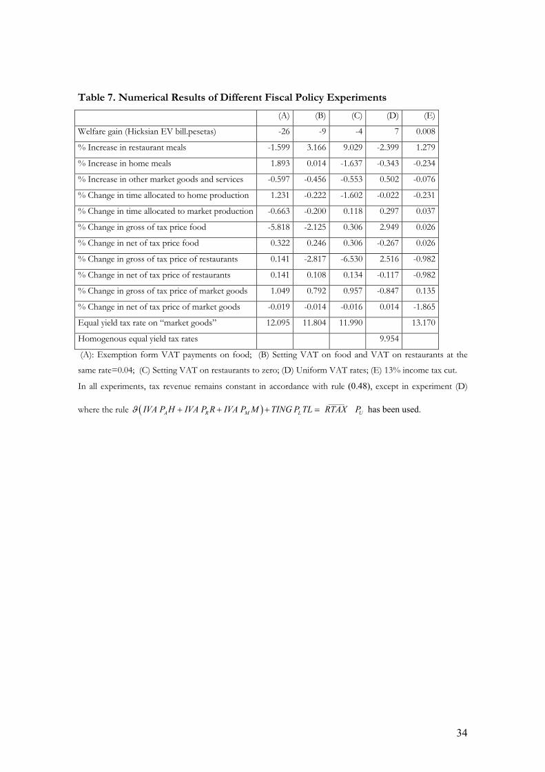
Table 7 displays the results in the variables of interest for the different tax policy
experiments. The motivation of the exercise is to quantify on the basis of data some of the
results previously addressed by the literature. An striking point is that any sensible
departure from the present tax scheme would only provoke slight welfare effects, as
measured as equivalent variations between two utility curves, indicating a tight design of
the tax structure in this simple version of the Spanish economy.
The first column deals with the food exemption case. This experiment is based on the
experience of other countries whose fiscal system does not levy tax on food, as is the case
of most of the US states, Canada, the United Kingdom and Mexico. The exercise throw
some light in the debate over the convenience of introducing the exemption on food in
Spain. The results show that the exemption of VAT on food in Spain would reduce
aggregate well-being by an equivalent of approximately 26 billion pesetas. As a result of the
change in taxation, household production of meals would increase by 1.9% and home time
by 1.2%, but restaurant production of meals would drop by 1.6% and total time allocated
to market production would also fall.
{Insert Table 7}
In the second experiment, effective VAT rates on food and restaurants are equalled to a
super reduced rate of 4%. In view of the fact that both rates in the benchmark are close to
the one simulated, the effects detected are minimal, although a slight decrease in efficiency
does seem to be confirmed. In this case both, restaurant and home meals increase, but
labor for home and market production is reduced due to a substitution of food for labor,
and also, for the market case, to a lower demand of “other market goods and services”.
In third place, we set to zero the VAT rate on restaurant meals. In this case the well being
also falls although the effect is even tinier. The labor supplied to the market increases
slighltly at the expense of a bigger fall of time devoted to home production.
22
In the column (D), the simulation sets a uniform VAT rate for all goods and services. The
equal yield flat VAT rate for this simple version of the Spanish economy is shown to be
about 10%. As a result of changes in prices, well-being increases by an equivalent of 7
billion pesetas with respect to the base case. While there is practically no effect on
household production, the production of meals in restaurants falls by 2.4%, while the
production of other market goods rises by 0.5 percentage points.
The last experiment from Table 4 captures the effects of a 13% income tax cut, offset by
an increase in effective VAT rates. A cut of 13% was considered because this is the
estimated decrease, according to the Instituto de Estudios Fiscales (Institute for Fiscal Studies
in Spain) in the average effective rate as a result of the last income tax reform bill. Results
show that this measure is neutral in efficiency. The main beneficiaries of this measure are
the restaurants that reduce the prices and increase the production.
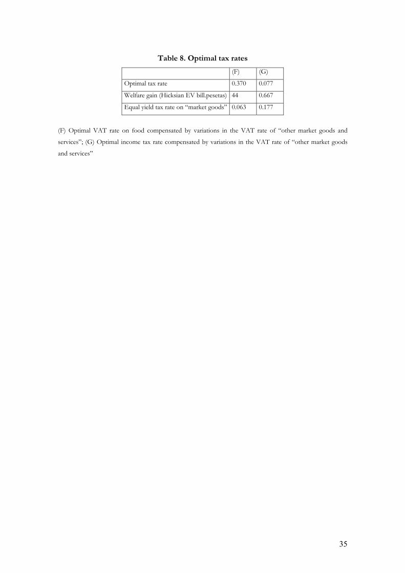
4.3 Optimal analysis
The above results are a consequence of isolated experiments that are reflected by the
unique changes in certain exogenous parameters of the model related to taxes. However,
it is also of interest, with the model at hand, to tackle the issue of optimal taxation. Table 8
display the results for two optimal exercises. In column (F) we maintain fixed the VAT rate
on restaurant meals, change the rate on food and offset by an equal yield VAT on “other
market goods and services” to obtain the combination that maximizes the welfare with
respect to the initial situation. For this to be achieved, the general equilibrium
corresponding to the different VAT rates has been obtained and the response of aggregate
well-being has been analysed. Results indicate an optimal VAT rate on food of 0.35, much
higher than the average tax rate on market goods. In column (G) we perform a similar
experiment for the income tax rate. It is shown that, starting at current levels, lowering the
tax on income and increasing the VAT on market goods would be optimal, although the
effects on welfare would be almost negligible.
{Insert Table 8}
23
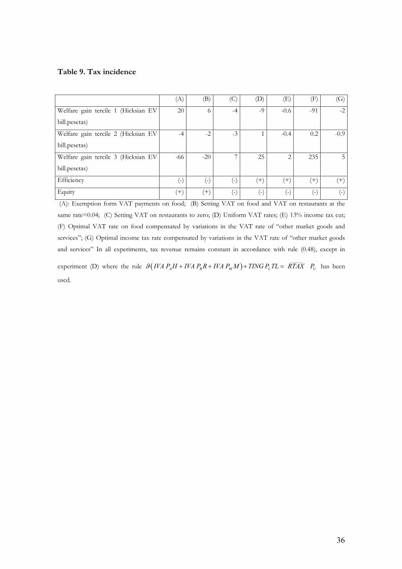
4.4 Tax incidence analysis
Tax analysis when household production is present has mainly focused in the simple case
of a representative consumer. However, a government may wish to sacrifice some
efficiency in exchange of a more equitable distribution of income. Therefore an important
question for tax policy making is the measure of the incidence of the tax, that is, the
distribution of the welfare effects within a population. In fact, distributional and efficiency
reasons work sometimes in opposite directions (see Auerbach and Hines, 2002). A
distributional theoretical framework when households can substitute away from market
expenditures towards time spent in home production was sketch by Sandmo (1990) but has
not found a conclusive empirical support in general equilibrium computational techniques.
Kleven et al (2000) emphasize the ambiguous implications that heterogeneity across
households could have for the optimal taxation of services, due in part to the different
weight of household production in high-income and low-income households.
In Table 9 we introduce household heterogeneity for illuminating the distributional fairness
of the fiscal experiments above when the representative consumer of this very simple
version of the Spanish economy is split up into three different groups according to terciles
of income, with the first tercile representing the lower income group. The elasticities of
substitution of the three groups are set equal to the ones of the representative consumer,
the difference being in the factor endowment different and preferences yielding different
combinations between leisure, market consumption and household production6.
The results show that all the fiscal experiments affect primarily to the low and top end of
the income distribution, and the most important, in almost all the cases the sign of the
efficiency effect is compensated by an opposite sign in equity. The only exception occurs
when the VAT on restaurants is set to zero, in this case both efficiency and equity are
penalized meaning that, according with this simple model, there is no argument at all for a
restaurant exemption to be carried out. Conversely, the food exemption, although brings
down global welfare, implies a positive redistribution of the tax burden, whereas the
optimal taxation on food heavily affect in a negative way the fairness.
{Insert Table 9}
6 We maintain the assumption of an identical household production technology for each household.
24
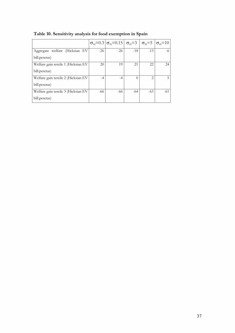
A sensitivity analysis (Table 10) confirms that the distributional impact of the food
exemption does not depend on the elasticity of substitution between time and food in
household production and the trade-off between efficiency and equity tend to disappear
the higher the value of the elasticity is. Thus, as the value of this parameter goes up, the
reasons against food exemption becomes more tenuous. This result points (as always) to
the importance of reliable econometric estimations of some key parameters.
{Insert Table 10}
5. Conclusions
Measuring the potential effects of fiscal reforms in the real-world with heterogeneity in the
population and a variety of pre-existing distortions have been a recurrent subject in public
finance. The numerical simulation techniques and, particularly, computable general
equilibrium models, have contributed to bridge the gap between economic theory and real-
world policy analysis. The household production theory has provided many interesting
applications to the theory of taxation, but the implementation of the household production
approach has not been addressed in a CGE model, due in part to the important statistical
requirements implied, that can be condensed in the so called social accounting matrices.
Recently we are witnessing in Europe a renewed interest in social accounting matrices. One
example is the Leadership Group on Social Accounting Matrices (SAM-LEG), that was born
under the statistical requirements for the implementation of the third phase of the
European Monetary Union and has prepared the guidelines for the construction of social
accounting matrices (see SAM-LEG, 2003). Other example is the first estimation of Tjeerd
et al (2004) of a SAM for the eurozone.
The contribution of this paper has been twofold: there is a methodological contribution
and there are some applications. In a methodological sense we illustrate how augmenting
standard social accounting matrices to include household production increases the
information available to the government and widen the room for maneuver in economy-
wide tax policy analysis. In the applications we take as the story line the model of Iorwerth
and Whalley (2002) replicating some of their results and confirming the key importance of
the elasticity of substitution between time and food in the elaboration of meals at home.
Then we take Spanish data and perform different tax policy experiments that underpins IW
results. Lastly we enlarge the number of consumers to establish some distributional results.
25
We show that in most of the cases efficiency and fairness act in opposite directions, and
that for the food exemption case, an increase in the key parameter reduce the efficiency
loses but does not change the positive distributional effects. Although the representation of
the economy has been kept in a very stylized way, the paper aims to transmit the usefulness
of extending the standard social accounting matrix framework to include the large amount
of the household production of goods and services for own final use.
Some suggested follow-ups to this research are straightforward with the information at
hand and aim to a more realistic representation of the economy, by means of the
incorporation of capital and different intermediate inputs, both in the market and in the
household production, the enlargement in the number of consumers, and the consideration
of different household production functions with different technologies across households.
The distribution of home-production skills across households has been pointed out by
Anderberg and Balestrino (2000) as possible extensions of their framework. Also Kleven
(2004) highlights the importance of combining consumption expenditures and time
allocation to implement its inverse factor share rule. Extending social accounting matrices
to include household production lay the foundations for all that issues to be feasible.
26
References
Anderberg, D. and A. Balestrino (2000): “Household production and the design of the tax
structure" International Tax and Public Finance, 7(4), pp. 563-84.
Auerbach, A. J. and J. R. Hines Jr. (2002): “Taxation and economic efficiency”. In
Auerbach, A. J. and M. Feldstein (Ed.): Handbook of Public Economics. North-Holland.
Balistreri, E. (2002): “Operationalizing equilibrium unemployment: a general equilibrium
external economies approach”. Journal of Economic Dyamics and Control, 26, pp. 347-374
Becker, G. (1965): “A theory of the allocation of time”. Economic Journal, 75, 493-517.
Boskin, M. J. (1975): “Efficiency aspects of the differential tax treatment of market and
household economic activity”. Journal of Public Economics, 4, pp. 1-25
Bourguignon, F. and A. Spadaro (2004): “Microsimulation as a Tool for Evaluating
Redistribution Policies: Theoretical Background and Empirical Applications”. Journal of
Economic Inequality. Forthcoming
Fullerton, D. and G. E. Metcalf (2002): “The distribution of tax burdens: an introduction”.
NBER Working Paper Series, 8978, pp. 1-27.
Gronau, R. (1977): “Leisure, home production and work-the theory of the allocation of
time revisited”. Journal of Political Economy, 85, pp. 1099-1123.
Gronau, R. (1997): “The theory of home production – the past ten years”. Journal of Labor
Economics, 15, 197-205.
Iorwerth, A. and J. Whalley (2002): “Efficiency considerations and the exemption of food
from sales and value added taxes”. Canadian Journal of Economics, 35, pp. 167-182
Kleven, H. J.; Richter, W. F. and P. B. Sorensen (2000): "Optimal Taxation with
Household Production". Oxford Economic Papers, 52, pp. 584-594
Kleven, H. J. (2004): “Optimal taxation and the allocation of time”. Journal of Public
Economics, 88, pp. 545-557.
Mathiesen, I. (1985): “Computation of economic equilibrium by a sequence on linear
complementarity problem”. Mathematical Programming Study, 23, pp. 144-162.
27
Piggott, J. and J. Whalley (1996): “The tax unit and household production”. Journal of
Political Economy, 104, pp. 398-418.
Piggott, J. and J. Whalley (2001): “VAT base broadening, self supply, and the informal
sector”. American Economic Review, 91, pp. 1084-1094.
Pyatt, G. (1990): “Accounting for time use”. Review of Income and Wealth, 36, pp. 33-52.
Rutherford, T. F. (1999): “ Applied general modeling with MPSGE as a GAMS subsystem:
an overview of the modeling framework and syntax”. Computational Economics, 14, pp. 1-49.
SAM-LEG (2003): Handbook on social accounting matrices and labor accounts. Pupulations and
social conditions 3/2003/E/N 23, Eurostat, Luxemburgo.
Sandmo, A. (1990): “Tax distorsions and household production”. Oxford Economic Papers,
42, pp. 78-90.
Shoven, J. B. and J. Whalley (1992): Applying general equilibrium. Cambridge University Press.
Cambridge.
Tjeerd, J.; Keuning, S.; McAdam, P. y R. Mink (2004): “Developing a Euro Area
accounting matrix: issues and applications”. European Central Bank. Working Paper Series Nº
356, May, pp 1-52.
Uriel, E.; Ferri, J. and M.L. Moltó (2005): “Estimation of an extended SAM with household
production for Spain, 1995”. IVIE WP.
28
TABLES
Table 1. Basic Social Accounting Matrix with household production for Spain
Home M. Prod. Restaur H.Meals Food M. labour H. labour Labour Leisure F. endow VAT Inc. tax
Home 186,611 5,492 5,830
M. prod. 47,195
Restaur 6,420
H. meals 18,612
Food 2,803 6,860
M. labour 42,551 3,189
H. labour 11,752
Labour 39,910 11,752
Leisure 125,706
F. endow 9,243 51,662 125,706
VAT 4,644 428 420
TING 5,830
Billions of pesetas
29
Table 2. Matrix micro-consistent with the mixed complementarity problem for
Spain
M R H U TL V CONS
PM 42,551 -42,551
PR 5,292 -5,992
PH 18,612 -18,612
PLO -11,752 -125,706 -39,910 177,386
PL -42,551 -3,189 45,740
PA -2,803 -6,440 9,243
PU 197,933 -197,933
PG -186,611 186,611
VAT -0,420 -5,072 5,492
TING -5,830 5,830
Billions of Pesetas
30
Table 3. Matrix micro-consistent with the mixed complementarity problem for
Canada
M R H U V CONS
PM 335 -335
PR 15 -15
PH 125 -125
PL -335 -10 -86 -625 1056
PA -5 -39 44
PU 1152.5 -1152.5
PG -1100 1100
VAT -52.5 52.5
Billions of dollars
31
Table 4. Basic social accounting matrix with household labour and household’s detail for Spain
Home
Tercil 1 Tercil 2 Tercil 3 M. Prod. Restaur H.Meals Food M.
labour H.
labour Labour Leisure F. endow VAT TING
Tercil 1 51,138 666 392 Tercil 2 60,660 1,505 1.197
Hom
e
Tercil 3 74,813 3,321 4.241 M. prod. 6.115 13,046 28,034 Restaur 593 1,658 4,169 H. meals 6.262 5,456 6,894 Food 2,803 6,860 M. labour 42,551 3,189 H. labour 11,752 Labour 39,910 11,752 Leisure 39.226 43,202 43,278 F. endow 9,243 51,662 125,706 VAT 4,644 428 420 TING 5,830 Billions of pesetas
Home: Representative household; M. prod: “market goods”; Restaur: restaurant meals; H. Meals: Home meals; M. labour: Market labour; H.
labour: Home labour; F. endow.: Factorial endowment; VAT: Revenue from VAT; Inc.tax: Revenue from income tax
32
Table 5. Substitution elasticities used in the calibration
Elasticity Value
Transformation elasticity between food and units of effective labour (ε) 5.0
Substitution elasticity between food and labour in restaurant production (σR) 0.3
Substitution elasticity between food and labour in home production (σH) 0.3
Substitution elasticity between restaurant meals and homemade meals in consumption (σS) 1.5
Substitution elasticity between leisure and consumption (σL) 0.2
Substitution elasticity between meals and “market goods” (σM) 0.6
33
Table 6. Simulation results compared with I-W
Model results
Iorweth-Whalley (1)
σH=0.15 σH=3 σH=5 σH=10
Welfare gain (Hicksian EV in 1992 $bill)
0.15 0.15 0.16 -0.04 -0.13 -0.24
Optimal tax rate 23.0% 23.0% 28.3% 5.2% 3.6% 2.4% Equal yield tax rate on food 13.4% 13.3% % Increase in restaurant meals
5.39% 5.59%
% Increase in home meals -2.87% -2.86% % Change in net of tax price food
-0.84% -0.8%
% Change in gross of tax price food
12.48% NA
% Change in net of tax price of restaurants
-0.28% NA
% Change in gross of tax price of restaurants
-1.63% -1.8%
% Change in time allocated to home production
-1.76% -1.76%
(1) Iorwerth and Whalley (2002). Table 2 page 174 NA: Non available
34
Table 7. Numerical Results of Different Fiscal Policy Experiments (A) (B) (C) (D) (E)
Welfare gain (Hicksian EV bill.pesetas) -26 -9 -4 7 0.008
% Increase in restaurant meals -1.599 3.166 9.029 -2.399 1.279
% Increase in home meals 1.893 0.014 -1.637 -0.343 -0.234
% Increase in other market goods and services -0.597 -0.456 -0.553 0.502 -0.076
% Change in time allocated to home production 1.231 -0.222 -1.602 -0.022 -0.231
% Change in time allocated to market production -0.663 -0.200 0.118 0.297 0.037
% Change in gross of tax price food -5.818 -2.125 0.306 2.949 0.026
% Change in net of tax price food 0.322 0.246 0.306 -0.267 0.026
% Change in gross of tax price of restaurants 0.141 -2.817 -6.530 2.516 -0.982
% Change in net of tax price of restaurants 0.141 0.108 0.134 -0.117 -0.982
% Change in gross of tax price of market goods 1.049 0.792 0.957 -0.847 0.135
% Change in net of tax price of market goods -0.019 -0.014 -0.016 0.014 -1.865
Equal yield tax rate on “market goods” 12.095 11.804 11.990 13.170
Homogenous equal yield tax rates 9.954
(A): Exemption form VAT payments on food; (B) Setting VAT on food and VAT on restaurants at the
same rate=0.04; (C) Setting VAT on restaurants to zero; (D) Uniform VAT rates; (E) 13% income tax cut.
In all experiments, tax revenue remains constant in accordance with rule (0.48), except in experiment (D)
where the rule ( )______
A R M L UIVA P H IVA P R IVA P M TING P TL RTAX Pϑ + + + = has been used.
35
Table 8. Optimal tax rates
(F) (G)
Optimal tax rate 0.370 0.077
Welfare gain (Hicksian EV bill.pesetas) 44 0.667
Equal yield tax rate on “market goods” 0.063 0.177
(F) Optimal VAT rate on food compensated by variations in the VAT rate of “other market goods and
services”; (G) Optimal income tax rate compensated by variations in the VAT rate of “other market goods
and services”
36
Table 9. Tax incidence
(A) (B) (C) (D) (E) (F) (G)
Welfare gain tercile 1 (Hicksian EV
bill.pesetas)
20 6 -4 -9 -0.6 -91 -2
Welfare gain tercile 2 (Hicksian EV
bill.pesetas)
-4 -2 -3 1 -0.4 0.2 -0.9
Welfare gain tercile 3 (Hicksian EV
bill.pesetas)
-66 -20 7 25 2 235 5
Efficiency (-) (-) (-) (+) (+) (+) (+)
Equity (+) (+) (-) (-) (-) (-) (-)
(A): Exemption form VAT payments on food; (B) Setting VAT on food and VAT on restaurants at the
same rate=0.04; (C) Setting VAT on restaurants to zero; (D) Uniform VAT rates; (E) 13% income tax cut;
(F) Optimal VAT rate on food compensated by variations in the VAT rate of “other market goods and
services”; (G) Optimal income tax rate compensated by variations in the VAT rate of “other market goods
and services” In all experiments, tax revenue remains constant in accordance with rule (0.48), except in
experiment (D) where the rule ( )______
A R M L UIVA P H IVA P R IVA P M TING P TL RTAX Pϑ + + + = has been
used.
37
Table 10. Sensitivity analysis for food exemption in Spain
σH=0.3 σH=0.15 σH=3 σH=5 σH=10
Aggregate welfare (Hicksian EV
bill.pesetas)
-26 -26 -18 -13 -6
Welfare gain tercile 1 (Hicksian EV
bill.pesetas)
20 19 21 22 24
Welfare gain tercile 2 (Hicksian EV
bill.pesetas)
-4 -4 0 2 5
Welfare gain tercile 3 (Hicksian EV
bill.pesetas)
-66 -66 -64 -63 -61

38