timedependent dike propagation from joint inversion of seismicity

JOURNAL OF GEOPHYSICAL RESEARCH: SOLID EARTH, VOL. 118, 1–20, doi:10.1002/2013JB010251, 2013

Time-dependent dike propagation from joint inversion of seismicityand deformation dataP. Segall,1 A. L. Llenos,1,2 S.-H. Yun,3 A. M. Bradley,1 and E. M. Syracuse4,5

Received 1 April 2013; revised 17 October 2013; accepted 22 October 2013.

[1] Dike intrusions both deform Earth’s surface and induce propagating earthquakeswarms. We develop methods to utilize both deformation and seismicity from brittle,volcano-tectonic earthquakes to image time-dependent dike propagation. Dieterich’s(1994) seismicity-rate theory is used to relate dike-induced stress changes to seismicityrate and is combined with elastic Green’s functions relating dike opening to deformation.Different space-time patterns of seismicity develop if earthquakes occur at the same depthas the dike compared to above/below the dike. In the former, seismicity initiates near thedike’s leading edges but shuts off as the dike tips pass and seismogenic volumes fall intostress shadows. In the latter, seismicity continues at a decaying rate after the tips pass. Wefocus on lateral propagation and develop a nonlinear inversion method that estimates dikelength and pressure as a function of time. The method is applied to the 2007 Father’s Dayintrusion in Kilauea Volcano. Seismicity is concentrated at �3 km depth, comparable togeodetic estimates of dike depth, and decays rapidly in time. With lateral propagationonly and a vertical dike-tip line, it is difficult to fit both GPS data and the rapid down-riftjump in seismicity, suggesting significant vertical propagation. For the events to haveoccurred below the dike requires a very short aftershock decay time, hence unreasonablyhigh background stressing rate. The rapid decay is better explained if the dike extendssomewhat below the seismicity. We suggest that joint inversion is useful for studying thediking process and may allow for improved short-term eruption forecasts.Citation: Segall, P., A. L. Llenos, S.-H. Yun, A. M. Bradley, and E. M. Syracuse (2013), Time-dependent dike propagation fromjoint inversion of seismicity and deformation data, J. Geophys. Res. Solid Earth, 118, doi:10.1002/2013JB010251.

1. Introduction[2] Seismicity and ground deformation are the two most

important geophysical methods for monitoring volcanoes.Yet, these data are essentially never combined in a quanti-tative manner for monitoring purposes. We suggest that arigorous method for jointly analyzing seismic and deforma-tion data could lead to improved eruption forecasts. Becausethe geometry of dikes is relatively well defined by bothgeologic and geophysical observations, they offer the mostpromising target for joint deformation and seismic anal-ysis. Dike intrusions cause stress changes and thus notonly deform the Earth’s surface but also commonly induce

1Department of Geophysics, Stanford University, Stanford, California,USA.

2Now at Earthquake Science Center, US Geological Survey, MenloPark, California, USA.

3Jet Propulsion Laboratory, California Institute of Technology,Pasadena, California, USA.

4Department of Geoscience, University of Wisconsin, Madison,Wisconsin, USA.

5Now at Los Alamos National Laboratory, Los Alamos, New Mexico,USA.

Corresponding author: P. Segall, Department of Geophysics, StanfordUniversity, Mitchell Bldg., 397 Panama Mall, Stanford, CA 94305-2215,USA. ([email protected])

©2013. American Geophysical Union. All Rights Reserved.2169-9313/13/10.1002/2013JB010251

propagating swarms of earthquakes. In this paper wedevelop a method that utilizes seismicity and geodetic datain a joint inversion to model dike propagation. The inver-sion provides time-dependent estimates of dike geometryand excess magma pressure (magma pressure in excess ofthe dike normal compressive stress). Equally importantly,the inversion methodology allows us to test competing mod-els for dike-induced earthquakes by examining goodness offit to both geodetic and seismic observations.

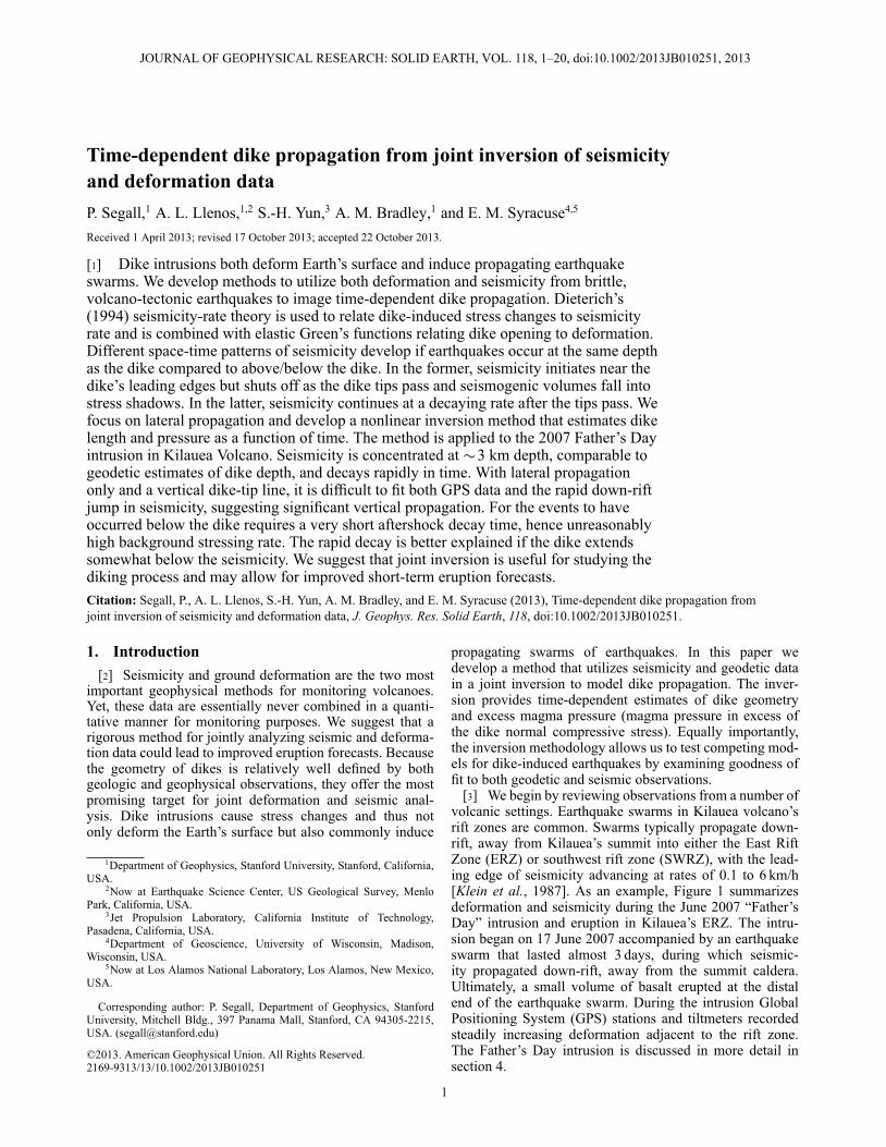
[3] We begin by reviewing observations from a number ofvolcanic settings. Earthquake swarms in Kilauea volcano’srift zones are common. Swarms typically propagate down-rift, away from Kilauea’s summit into either the East RiftZone (ERZ) or southwest rift zone (SWRZ), with the lead-ing edge of seismicity advancing at rates of 0.1 to 6 km/h[Klein et al., 1987]. As an example, Figure 1 summarizesdeformation and seismicity during the June 2007 “Father’sDay” intrusion and eruption in Kilauea’s ERZ. The intru-sion began on 17 June 2007 accompanied by an earthquakeswarm that lasted almost 3 days, during which seismic-ity propagated down-rift, away from the summit caldera.Ultimately, a small volume of basalt erupted at the distalend of the earthquake swarm. During the intrusion GlobalPositioning System (GPS) stations and tiltmeters recordedsteadily increasing deformation adjacent to the rift zone.The Father’s Day intrusion is discussed in more detail insection 4.

1

SEGALL ET AL: TIME-DEPENDENT DIKE PROPAGATION

−155.25 −155.2 −155.15 −155.1 −155.0519.25

19.3

19.35

19.4

19.45

19.5

Latit

ude

Longitude

GOPM

KTPM

NUPM

PGF2

HALRESC

POO

10 cm

20 µrad

17.5 18 18.5 19

−155.24

−155.22

−155.2

−155.18

−155.16

−155.14

Day in June 2007

Long

itude

A

B

µrad

5 km

Figure 1. (a) Map showing the island of Hawaii (inset)and Kilauea’s East Rift Zone. Dots indicate relocated earth-quakes (color indicates timing according to the intrusionchronology of Poland et al. [2008], with red betweendays 17.51 and 17.73, green between days 17.73 and 17.79,and blue between days 17.79 and 18.7). Vectors indicatecumulative observed displacement and tilt (dashed). (b)Space-time evolution of the seismicity during the intrusion.

[4] Accurate earthquake locations derived using wave-form cross correlation during the 1983 intrusion that initi-ated the ongoing Pu’u ’O’o eruption reveal an extremelynarrow 16 km long zone at a depth of 3–4 km within theERZ [Rubin et al., 1998]. The leading edge of seismicityextended down-rift at a rate of � 0.7 km/h. The swarm wasaccompanied by a sequence of tilt changes consistent witha laterally propagating opening dislocation [Okamura et al.,1988]. These observations confirm that deformation andseismicity represent different responses to the same underly-ing physical process. Geodetic observations in 1983 providelimited constraint on the depth of intrusion but are gener-ally consistent with dike opening from near Earth’s surfaceto a depth of 3.0 to 4.5 km [Wallace and Delaney, 1995].Subsequent intrusions in the middle ERZ captured by GPSand more recently interferometric synthetic aperture radar(InSAR) observations in 1997, 1999, and 2007 extended to

depths of roughly 2.5 ˙ 1 km [Owen et al., 2000a; Cervelliet al., 2002; Montgomery-Brown et al., 2010]. In summary,within considerable uncertainties the depths of the 1983swarm earthquakes are consistent with the bottoms of ERZdike intrusions inferred from geodetic data.

[5] The most obvious explanation for the narrow depthextent of dike-induced earthquakes on Kilauea is that theseismicity is controlled by strong stress concentrations at thedike bottoms. This view is supported by the general agree-ment between the geodetically inferred depth extent of dikeopening and the depth of swarm seismicity. However, ifthe depth extent of diking is controlled by a temperature-dependent brittle-ductile transition, such that dikes extendpartially into deeper ductile rock, the background devia-toric stresses at dike bottoms may be insufficient to generateearthquakes [Rubin et al., 1998]. In this case the narrowdepth extent of seismicity could be controlled by strongstress concentrations at the top of a deep rift body, which isestimated to occur at � 3 km depth [Delaney et al., 1990;Owen et al., 2000b]. These effects are not independent; itis likely that both the top of deep rift opening and the bot-tom of episodic dike intrusions are ultimately controlled by atemperature-dependent rheological transition and associatedbackground stress distributions. Thus, the stress concentra-tions due to diking as well as deep rift opening are likely tooccur at comparable depths.

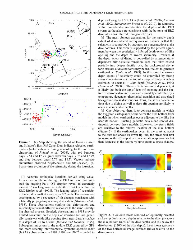
[6] One objective, then, is to contrast models in whichthe triggered earthquakes occur below the dike bottom frommodels in which earthquakes occur adjacent to the dike butnear its bottom. Existing geodetic data alone cannot dis-tinguish between these models. However, the stress fieldsare sensitive to the relative location of the dike bottom(Figure 2). If the earthquakes occur in the crust adjacentto the dike but above its lower tip line, the stress will firstincrease as the dike-tip stress concentration approaches butthen decrease as the source volume enters a stress shadow.

A)

B)

Figure 2. Coulomb stress resolved on optimally orientedstrike-slip faults at two depths relative to the dike: (a) abovethe dike bottom (80% of the dike depth), and (b) below thedike bottom (120% of the dike depth). Inset shows geometryof the two horizontal image surfaces (blue) relative to thedike (green).

2


A) B)

C)

Afar 2007 Afar 2007

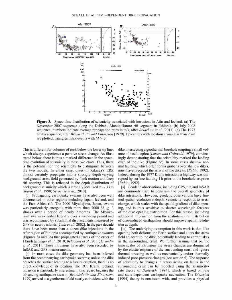
Figure 3. Space-time distribution of seismicity associated with intrusions in Afar and Iceland. (a) TheNovember 2007 sequence along the Dabbahu-Manda-Hararo rift segment in Ethiopia. (b) July 2008sequence; numbers indicate average propagation rates in m/s, after Belachew et al. [2011]. (c) The 1977Krafla sequence, after Brandsdottir and Einarsson [1979]. Epicenters with location errors less than 2 kmare plotted; triangles mark events with M � 3.

This is different for volumes of rock below the lower tip line,which always experience a positive stress change. As illus-trated below, there is thus a marked difference in the space-time evolution of seismicity in these two cases. Thus, thereis the potential for the seismicity to distinguish betweenthe two models. In either case, dikes in Kilauea’s ERZalmost certainly propagate into a strongly depth-varyingbackground stress field generated by flank motion and deeprift opening. This is reflected in the depth distribution ofbackground seismicity which is strongly localized at� 3 km[Rubin et al., 1998; Syracuse et al., 2010].

[7] Propagating earthquake swarms have also been welldocumented in other regions including Japan, Iceland, andthe East Africa rift. The 2000 Miyakejima, Japan, swarmwas particularly energetic with more than 7000 M � 3shocks over a period of nearly 2 months. The Miyake-jima swarm extended laterally over a weeklong period andwas accompanied by substantial displacements measured byGPS on nearby islands [Toda et al., 2002]. In the past decadethere have been more than a dozen dike injections in theAfar region of Ethiopia accompanied by earthquake swarms(Figures 3a and 3b) that propagated at rates of the order of1 km/h [Ebinger et al., 2010; Belachew et al., 2011; Grandinet al., 2011]. These intrusions have also been recorded byInSAR and GPS measurements.

[8] In most cases the dike geometry has been inferredfrom the accompanying earthquake swarms; unless the dikebreaches the surface leading to a fissure eruption, there is nodirect knowledge of its location. The 1977 Krafla, Iceland,intrusion is particularly interesting in this regard because theadvancing earthquake swarm [Brandsdottir and Einarsson,1979] arrived at a geothermal field nearly coincident with the

dike intersecting a geothermal borehole erupting a small vol-ume of basalt tephra [Larsen and Grönvold, 1979], convinc-ingly demonstrating that the seismicity marked the leadingedge of the dike (Figure 3c). In some cases shallow nor-mal faulting, which often forms grabens over shallow dikes,must have preceded the arrival of the dike tip [Rubin, 1992].Indeed, during the 1977 Krafla intrusion, a highway was dis-rupted by surface faulting 1 h prior to the borehole eruption[Rubin, 1992].

[9] Geodetic observations, including GPS, tilt, and InSARare commonly used to constrain the overall geometry ofdike intrusions. However, geodetic observations have lim-ited spatial resolution at depth. Seismicity responds to stresschange, which scales with the spatial gradient of dike open-ing, and is thus sensitive to shorter wavelength featuresof the dike opening distribution. For this reason, includingadditional information from the spatiotemporal distributionof dike-induced earthquakes should improve spatial resolu-tion at depth.

[10] The underlying assumption in this work is that dikeopening both deforms the Earth surface and alters the stressfield adjacent to the dike, potentially leading to earthquakesin the surrounding crust. We further assume that on thetime scales of intrusions the stress changes are dominatedby the elastic response of the surrounding crust and ignorethermal stressing as well as mechanically and/or thermallyinduced pore-pressure changes (see section 5). The responseof seismicity to changes in stress acting on faults in thesurrounding crust can be modeled using the seismicity-rate theory of Dieterich [1994], which is based on rateand state-dependent earthquake nucleation. The Dieterich[1994] theory is consistent with, and provides a physical

3


basis for, the Omori decay of aftershocks and has alreadybeen used to model seismicity-rate changes associated withdike intrusions [Dieterich et al., 2000, 2003, Toda et al.,2002] as well as slow slip events [Segall et al., 2006; Llenosand McGuire, 2011].

[11] Dieterich et al. [2000, 2003] used the theory ofDieterich [1994] to invert observed seismicity-rate changeson Kilauea’s south flank for stress changes within the vol-cano. They compared the inferred stress changes to thosecomputed independently from elastic models of surfacedeformation. While not a formal joint inversion of seismicand geodetic data as presented here, these papers showedthe power of analyzing both data types in a mechanicallyconsistent framework. In particular, Dieterich et al. [2003]showed that south flank seismicity in the 3 month period fol-lowing the 1983 ERZ dike injection requires a combinationof deep rift opening and slip on the south flank decollement.We compare these conclusions to our results in section 5.

[12] Segall and Yun [2005] demonstrated that a jointinversion of synthetic seismicity and InSAR data signifi-cantly improved the spatial resolution of a dike at depth,relative to inversion of InSAR data alone. In this paper, weexpand on that time-independent approach and develop amethod for time-dependent dike propagation [Llenos et al.,2010, 2011]. We use the Dieterich [1994] equations to relatestress changes caused by dike opening to seismicity-ratechanges and combine these with elastic Green’s func-tions to invert surface displacements and seismicity fordike length and pressure over time using a nonlinear leastsquares algorithm.

[13] The forward model specifies the spatially uniformexcess pressure acting on the dike walls [Yun et al.,2006]. This provides several advantages over kinematicapproaches, which employ spatial smoothing constraintsto regularize the inversion. Most importantly, the pressureboundary condition is motivated by the physics of the dikingprocess. Secondly, these boundary conditions require fewerdegrees of freedom in the inversion, compared to kinematicmodels in which the amount of opening on each patch ofa dike must be solved for at each time step, thus obviatingthe need for regularization. Finally, the estimated pressurehistory can provide direct insight into the physical processdriving the intrusion.

[14] We first review the method for forward simulationof deformation and seismicity and then introduce the inver-sion algorithm. After testing the method with simulated datawe apply it to the 2007 Father’s Day intrusion (Figure 1).The seismicity that occurred during the swarm is relo-cated and analyzed together with GPS and tiltmeter data[Montgomery-Brown et al., 2011]. Our results suggest thatthe rapid down-rift expansion of seismicity reflects an appar-ent velocity involving a significant vertical component ofdike propagation. The results are also sensitive to the verticalextent of dike opening relative to the earthquake depths andhave implications for the background stressing rate withinKilauea’s ERZ and along-strike variations in stressing andseismicity rates.

2. Method[15] We model a dike intrusion as a rectangular crack,

subjected to spatially uniform internal pressure, that

propagates in an elastic half-space. We expect lateral prop-agation to dominate for shallow intrusions and to be theeasiest to resolve, although future work should general-ize the approach to consider vertical propagation. We thusassume in this work that dike height, depth, strike, and dipremain constant, while the dike length and magma pres-sure change with time. We combine a forward model forseismicity rate based on integration of the Dieterich [1994]equations with elastic Green’s functions to invert surface dis-placements and seismicity for changes in dike length L andexcess magma pressure �p (magma pressure in excess ofdike-normal stress) over time. We also solve for the time-independent constitutive parameter a and the backgroundstressing rate Psr (both defined below).

2.1. Forward Modeling[16] We assume a uniform pressure boundary condition

on the dike walls. This cannot be the case at the dike tip[Rubin and Gillard, 1998; Rubin et al., 1998]; however, thespatial scale over which the dike-tip variations occur maybe sufficiently small that it influences the stress only in asmall volume around the dike tips. Future studies shouldinclude the influence of the dike-tip zone, as well as depthdependence of excess pressure (see section 5). At each timestep, the dike plane is subdivided into Nel grid elements,and the Boundary Element Method (BEM, specifically theDisplacement Discontinuity Method) is used to obtain thedike opening ı(�) appropriate for the specified dike pres-sure, where � is spatial coordinate on the dike plane. Theinduced normal stress on the dike elements is a linear func-tion of the dike opening; therefore, given the excess pressureboundary condition �p and the elastic response functions Arelating opening to normal traction in an isotropic, homoge-neous, linear-elastic half-space, the opening distribution canbe computed via

ı(�) = A–1�p, (1)

where �p is a constant vector of length Nel. The sur-face deformation d is computed from elastic Green’s func-tions G relating the dike opening to deformation [Okada,1992, e.g.,]:

d(x, tk) = G[L(tk), x; �]ı(�, tk) = G[L(tk), x; �]A–1�p(tk). (2)

The Green’s functions depend on the dike length L, strike,depth, and so on, although in this implementation onlylength changes with time. To predict seismicity triggered bystress changes induced by the dike, we utilize the seismicity-rate theory of Dieterich [1994]. The theory is based on thetime to instability of a population of independent sourcesthat slip according to a rate- and state-dependent friction lawand the assumption of constant seismicity rate under con-stant background stressing rate Psr. Specifically, the modelrelates the seismicity rate R to stress changes via

R =dNdt

=r� Psr

(3)

d�dt

=1

a�

�1 – �

dsdt

�, (4)

where N is the number of earthquakes, r is the backgroundseismicity rate, � is a state variable, a is a frictional con-stitutive parameter (related to the “direct effect” in rate

4


A)

C) D)

B)90

80

70

60

50

40

30

20

10 15 20 25 30

0

0 5 10 15 20 25 300 5

10 15 20 25 300 5-10

10

90

80

70

60

50

40

30

20

10

0

-10

90

80

70

60

50

40

30

20

10

-10

0

90

100

80

70

60

50

40

30

20

10

00 5 10 15 20

Sei

smic

ity R

ate,

1/h

rS

eism

icity

Rat

e, 1

/hr

Sei

smic

ity R

ate,

1/h

rS

eism

icity

Rat

e, 1

/hr

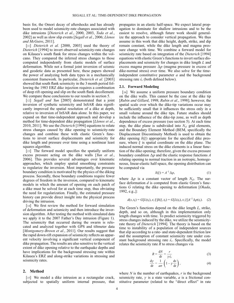
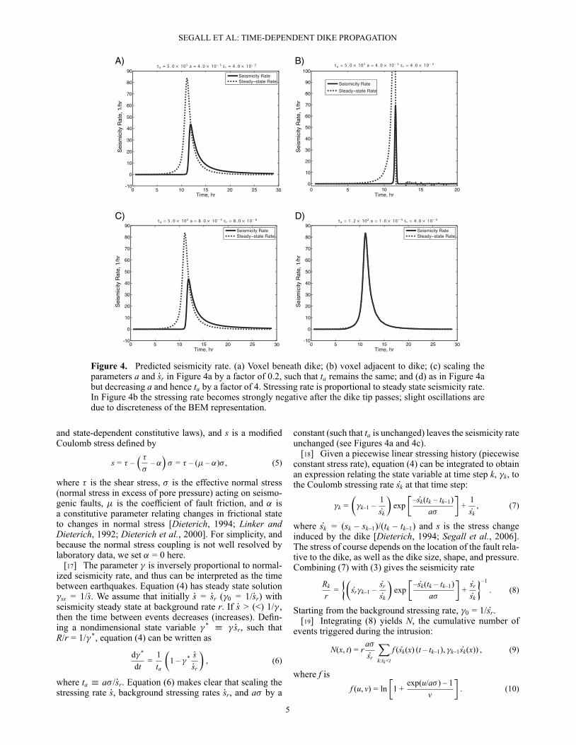
Figure 4. Predicted seismicity rate. (a) Voxel beneath dike; (b) voxel adjacent to dike; (c) scaling theparameters a and Psr in Figure 4a by a factor of 0.2, such that ta remains the same; and (d) as in Figure 4abut decreasing a and hence ta by a factor of 4. Stressing rate is proportional to steady state seismicity rate.In Figure 4b the stressing rate becomes strongly negative after the dike tip passes; slight oscillations aredue to discreteness of the BEM representation.

and state-dependent constitutive laws), and s is a modifiedCoulomb stress defined by

s = � –� ��

– ˛�� = � – (� – ˛)� , (5)

where � is the shear stress, � is the effective normal stress(normal stress in excess of pore pressure) acting on seismo-genic faults, � is the coefficient of fault friction, and ˛ isa constitutive parameter relating changes in frictional stateto changes in normal stress [Dieterich, 1994; Linker andDieterich, 1992; Dieterich et al., 2000]. For simplicity, andbecause the normal stress coupling is not well resolved bylaboratory data, we set ˛ = 0 here.

[17] The parameter � is inversely proportional to normal-ized seismicity rate, and thus can be interpreted as the timebetween earthquakes. Equation (4) has steady state solution�ss = 1/Ps. We assume that initially Ps = Psr (�0 = 1/Psr) withseismicity steady state at background rate r. If Ps > (<) 1/� ,then the time between events decreases (increases). Defin-ing a nondimensional state variable � * � � Psr, such thatR/r = 1/� *, equation (4) can be written as

d�*

dt=

1ta

�1 – �* Ps

Psr

�, (6)

where ta � a� /Psr. Equation (6) makes clear that scaling thestressing rate Ps, background stressing rates Psr, and a� by a

constant (such that ta is unchanged) leaves the seismicity rateunchanged (see Figures 4a and 4c).

[18] Given a piecewise linear stressing history (piecewiseconstant stress rate), equation (4) can be integrated to obtainan expression relating the state variable at time step k, �k, tothe Coulomb stressing rate Psk at that time step:

�k =��k–1 –

1Psk

�exp

�– Psk(tk – tk–1)

a�

�+

1Psk

, (7)

where Psk = (sk – sk–1)/(tk – tk–1) and s is the stress changeinduced by the dike [Dieterich, 1994; Segall et al., 2006].The stress of course depends on the location of the fault rela-tive to the dike, as well as the dike size, shape, and pressure.Combining (7) with (3) gives the seismicity rate

Rk

r=��Psr�k–1 –

Psr

Psk

�exp

�– Psk(tk – tk–1)

a�

�+Psr

Psk

–1

. (8)

Starting from the background stressing rate, �0 = 1/ Psr.[19] Integrating (8) yields N, the cumulative number of

events triggered during the intrusion:

N(x, t) = ra�Psr

Xk:tk<t

f ( Psk(x) (t – tk–1), �k–1 Psk(x)) , (9)

where f isf (u, v) = ln

�1 +

exp(u/a� ) – 1v

�. (10)

5


0 10 20 30−5000

0

5000

10000

15000

20000

Time

Dis

tanc

e

0 10 20 30−5000

0

5000

10000

15000

20000

Time

A) B)

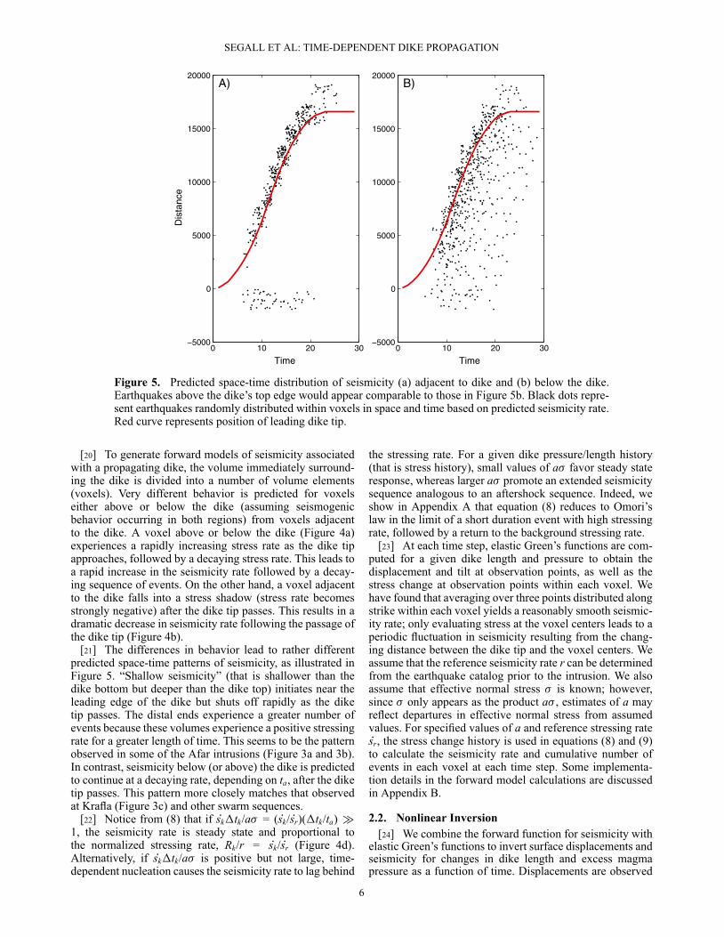
Figure 5. Predicted space-time distribution of seismicity (a) adjacent to dike and (b) below the dike.Earthquakes above the dike’s top edge would appear comparable to those in Figure 5b. Black dots repre-sent earthquakes randomly distributed within voxels in space and time based on predicted seismicity rate.Red curve represents position of leading dike tip.

[20] To generate forward models of seismicity associatedwith a propagating dike, the volume immediately surround-ing the dike is divided into a number of volume elements(voxels). Very different behavior is predicted for voxelseither above or below the dike (assuming seismogenicbehavior occurring in both regions) from voxels adjacentto the dike. A voxel above or below the dike (Figure 4a)experiences a rapidly increasing stress rate as the dike tipapproaches, followed by a decaying stress rate. This leads toa rapid increase in the seismicity rate followed by a decay-ing sequence of events. On the other hand, a voxel adjacentto the dike falls into a stress shadow (stress rate becomesstrongly negative) after the dike tip passes. This results in adramatic decrease in seismicity rate following the passage ofthe dike tip (Figure 4b).

[21] The differences in behavior lead to rather differentpredicted space-time patterns of seismicity, as illustrated inFigure 5. “Shallow seismicity” (that is shallower than thedike bottom but deeper than the dike top) initiates near theleading edge of the dike but shuts off rapidly as the diketip passes. The distal ends experience a greater number ofevents because these volumes experience a positive stressingrate for a greater length of time. This seems to be the patternobserved in some of the Afar intrusions (Figure 3a and 3b).In contrast, seismicity below (or above) the dike is predictedto continue at a decaying rate, depending on ta, after the diketip passes. This pattern more closely matches that observedat Krafla (Figure 3c) and other swarm sequences.

[22] Notice from (8) that if Psk�tk/a� = ( Psk/ Psr)(�tk/ta) �1, the seismicity rate is steady state and proportional tothe normalized stressing rate, Rk/r = Psk/ Psr (Figure 4d).Alternatively, if Psk�tk/a� is positive but not large, time-dependent nucleation causes the seismicity rate to lag behind

the stressing rate. For a given dike pressure/length history(that is stress history), small values of a� favor steady stateresponse, whereas larger a� promote an extended seismicitysequence analogous to an aftershock sequence. Indeed, weshow in Appendix A that equation (8) reduces to Omori’slaw in the limit of a short duration event with high stressingrate, followed by a return to the background stressing rate.

[23] At each time step, elastic Green’s functions are com-puted for a given dike length and pressure to obtain thedisplacement and tilt at observation points, as well as thestress change at observation points within each voxel. Wehave found that averaging over three points distributed alongstrike within each voxel yields a reasonably smooth seismic-ity rate; only evaluating stress at the voxel centers leads to aperiodic fluctuation in seismicity resulting from the chang-ing distance between the dike tip and the voxel centers. Weassume that the reference seismicity rate r can be determinedfrom the earthquake catalog prior to the intrusion. We alsoassume that effective normal stress � is known; however,since � only appears as the product a� , estimates of a mayreflect departures in effective normal stress from assumedvalues. For specified values of a and reference stressing ratePsr, the stress change history is used in equations (8) and (9)to calculate the seismicity rate and cumulative number ofevents in each voxel at each time step. Some implementa-tion details in the forward model calculations are discussedin Appendix B.

2.2. Nonlinear Inversion[24] We combine the forward function for seismicity with

elastic Green’s functions to invert surface displacements andseismicity for changes in dike length and excess magmapressure as a function of time. Displacements are observed

6


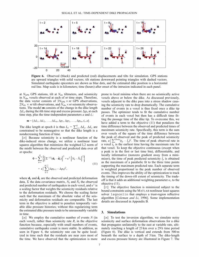
Figure 6. Observed (black) and predicted (red) displacements and tilts for simulation. GPS stationsare upward triangles with solid vectors; tilt stations downward pointing triangles with dashed vectors.Simulated earthquake epicenters are shown as blue dots, and the estimated dike position is a horizontalred line. Map scale is in kilometers; time (hours) after onset of the intrusion indicated in each panel.

at NGPS GPS stations, tilt at Ntilt tiltmeters, and seismicityin Nobs voxels observed at each of nt time steps. Therefore,the data vector consists of 3NGPS � nt GPS observations,2Ntilt � nt tilt observations, and Nobs�nt seismicity observa-tions. The model m consists of the change in the dike length�Lk during the kth time step and excess pressure�pk at eachtime step, plus the time-independent parameters a and Psr:

m = [�L1,�L2, : : : ,�Lnt,�p1,�p2, : : : ,�pnt, Psr, a] .

The dike length at epoch k is thus Lk =Pk

j=1�Lj. �Lj areconstrained to be nonnegative so that the dike length is anondecreasing function of time.

[25] Because seismicity is a nonlinear function of thedike-induced stress change, we utilize a nonlinear leastsquares algorithm that minimizes the weighted L2 norm ofthe misfit between the observed and predicted data over allnt epochs:

ˆ =ntX

k=1

�†–1/2(dk – Odk)2

+ �2Nk – ONk

2

+ �22

nt–1Xk=1

(�pk+1 –�pk)2,

(11)

where dk and Odk are the observed and predicted deformationdata, † the data covariance matrix, Nk and ONk the observedand predicted number of earthquakes in each voxel, and �2 isa scaling factor that weights the seismicity residuals relativeto the deformation residuals. We choose the scaling factorsuch that the maximum of the absolute value of the seis-micity and deformation residuals are comparable. The lastterm in the objective is added to penalize temporally vari-able dike pressure histories; without this regularizing termthe estimated dike pressure tends to be unreasonably variablein time.

[26] We employ the cumulative number of events N (ineach voxel), rather than seismicity rate R, in the objectivefunction because, especially with small numbers of events,cumulative earthquake count is more stable. In addition, asseen in Figure 4, the seismicity rate can be quite local-ized in time such that the residuals are near zero most ofthe time. We have observed that the optimization is more

prone to local minima when there are no seismically activevoxels above or below the dike. As discussed previously,voxels adjacent to the dike pass into a stress shadow caus-ing the seismicity rate to drop dramatically. The cumulativenumber of events in a voxel is thus fixed once a dike tippasses. The optimizer tends to fit the cumulative numberof events in each voxel but then has a difficult time fit-ting the passage time of the dike tip. To overcome this, wehave added a term to the objective (11) that penalizes thetime difference between the observed and predicted times ofmaximum seismicity rate. Specifically, this term is the sumover voxels of the square of the time difference betweenthe peak of observed and the peak of predicted seismicityrate, �2

3PNvox(tp – Otp)2. The time of peak observed rate in

a voxel tp is the earliest time having the maximum rate forthat voxel. To keep the objective continuous (except whena peak is in the first or last time bin), differentiable, andlocally informative (nonzero gradient away from a mini-mizer), the time of peak predicted seismicity Otp is obtainedas the maximum of a parabolic fit to the three time pointssupporting the maximum predicted rate. Each separate termis weighted proportional to the peak number of observedevents. This improves the ability of the optimization to trackthe timing of the down-rift extent of seismicity. The trade-off is that it adds an additional weighting parameter �3 to theobjective (11).

[27] The objective function is minimized subject to thebound constraints using the MATLAB nonlinear least squaressolver lsqnonlin that employs a trust-region reflectivealgorithm [Coleman and Li, 1996]. Some implementationdetails are discussed in Appendix B.

3. Simulations[28] To test the inversion algorithm, we simulate noisy

seismicity and surface deformation observations for a dikethat propagates unilaterally to the east at variable rate, ulti-mately reaching a length of 23 km over a 29 h time period(Figure 6). The dike is vertical and extends from 500 mbeneath the surface to a depth of 5 km. The dike-lengthand excess pressure history are illustrated in Figure 7. The

7


0 5 10 15 20 25 300

5

10

15

20

25

Dik

e Le

ngth

[km

]

A)

EstimateTrue

0 5 10 15 20 25 303456789

10

Pre

ssur

e [M

Pa]

Time [hrs]

B)

Deformation and Seismicity

0 5 10 15 20 25 300

5

10

15

20

25

Dik

e Le

ngth

[km

]

C)

EstimateTrue

0 5 10 15 20 25 302468

10121416

Pre

ssur

e [M

Pa]

Time [hrs]

D)

Seismicity Only

Figure 7. Comparison of input and estimated history of (top) dike length (km) and (bottom) excess dikepressure (MPa) for simulation. Simulations with (left) both geodetic and seismic data and (right) onlyseismicity data.

input dike pressure decreases as the magma chamber feed-ing the eruption drains and then slightly recovers after dikepropagation ceases (Figure 7).

[29] The simulated deformation data come from eightGPS receivers and four tiltmeters; locations are illustratedin Figure 6. Normally distributed random noise was addedto the synthetic data with a magnitude of 20% of the meanof the final GPS displacements and tilts. Seismic data weresynthesized in 98 voxels surrounding the dike. The refer-ence seismicity rate r is taken to be 0.002 events/h (one eventevery � 21 days); the reference stressing rate is Psr = 4 �10–5 MPa/h (0.35 MPa/yr). The effective normal stress � isuniformly 50 MPa, and the friction parameter a is 0.004. Thecharacteristic time ta is thus 5000 h or � 210 days. The sim-ulated seismicity was computed on vertical strike-slip faultsoriented 30ı counterclockwise from the dike plane, whilein the inversion it was assumed (incorrectly) that the faultswere oriented 30ı clockwise from the dike plane. Likewise,the coefficient of friction used to generate the data was 0.6,while in the inversion we assume 0.4. Noise in seismicitydata comes from imprecise earthquake locations. Randomevent locations were computed from the predicted seis-micity rate assuming a uniform spatial distribution withineach voxel. Random location errors were then assigned toeach event with a standard deviation of 0.75 km (compara-ble to the voxel dimensions) and the event count per voxelcomputed based on the perturbed locations.

[30] For the inversion the initial estimate was intention-ally set to be far from the true input model. The initialdike-length increments �Lk were 5% of the average incre-ment (total length divided by number of epochs), the dikepressure was initially set to 5% of the mean pressure, and Psrand a were perturbed by factors of 5. The lower and upperbounds on dike-length increment were set to 1 m and 25% ofthe final length, respectively. The dike pressure is boundedbetween zero and 3 times the maximum pressure, while thebounds on Psr and a were factors of 10 above and below thetrue value. Reasonable results are obtained with weights onthe seismic residuals 20% of the weight on the deforma-tion residuals (� = 0.2 in equation (11)). For � � 0.2 thedeformation data are essentially ignored. The constant for

smoothing the pressure differences was set to �2 = 10 basedon visual inspection.

3.1. Simulation Results[31] The estimated dike-length and pressure history are

shown in Figure 7 (left). The dike-length history is recoveredremarkably well. The excess dike pressure is underestimated(by about 20%) at early time but is reasonably well estimatedfor t � 7 h. At early times the dike is short and generatesrelatively little measurable deformation, and the pressureduring this period is thus poorly constrained. The inferreddike model does a good job of reproducing both the spatialand temporal pattern of displacements and tilts (Figure 6).A comparison between the input and estimated dike length,pressure, and seismicity is shown in Figure 8. The estimatedbackground stressing rate Psr is a factor of 1.5 greater than thetrue value, while the friction parameter a is 68% of the inputvalue. The ratio ta = a� / Psr is thus biased low by a factorof 2.3.

[32] The conclusion of this test is that the algorithmcan recover the dike-length and pressure history reasonablyaccurately even in the presence of significant noise, andwith some incorrect modeling assumptions about the faultplane orientations and coefficient of friction. Of course thisdoes not prove that additional assumptions, particularly thevalidity of the seismicity-rate model, are valid in the Earth.

[33] Before testing the method on actual data we per-form one additional test removing deformation data from theobjective function, so that the estimation is controlled com-pletely by seismicity. Results are shown in Figure 7 (right).The algorithm does a good job of recovering the dike lengthsimply from the migration of the earthquake swarm. With-out deformation data, the recovered excess magma pressureis inaccurate, as expected. The limited constraint on pressurearises because the stressing rate is a function of pressure.However, with a weaker constraint on pressure we expectthat the seismicity-rate parameters will be less well con-strained. This is indeed true; Psr is a factor of 3.5 greaterthan true, while a is a factor of 1.3 larger. The average dikepressure is also a factor of 2.0 (range 1.5 to 2.5) greaterthan the input, such that ta is biased low by a factor of 2.7.

8


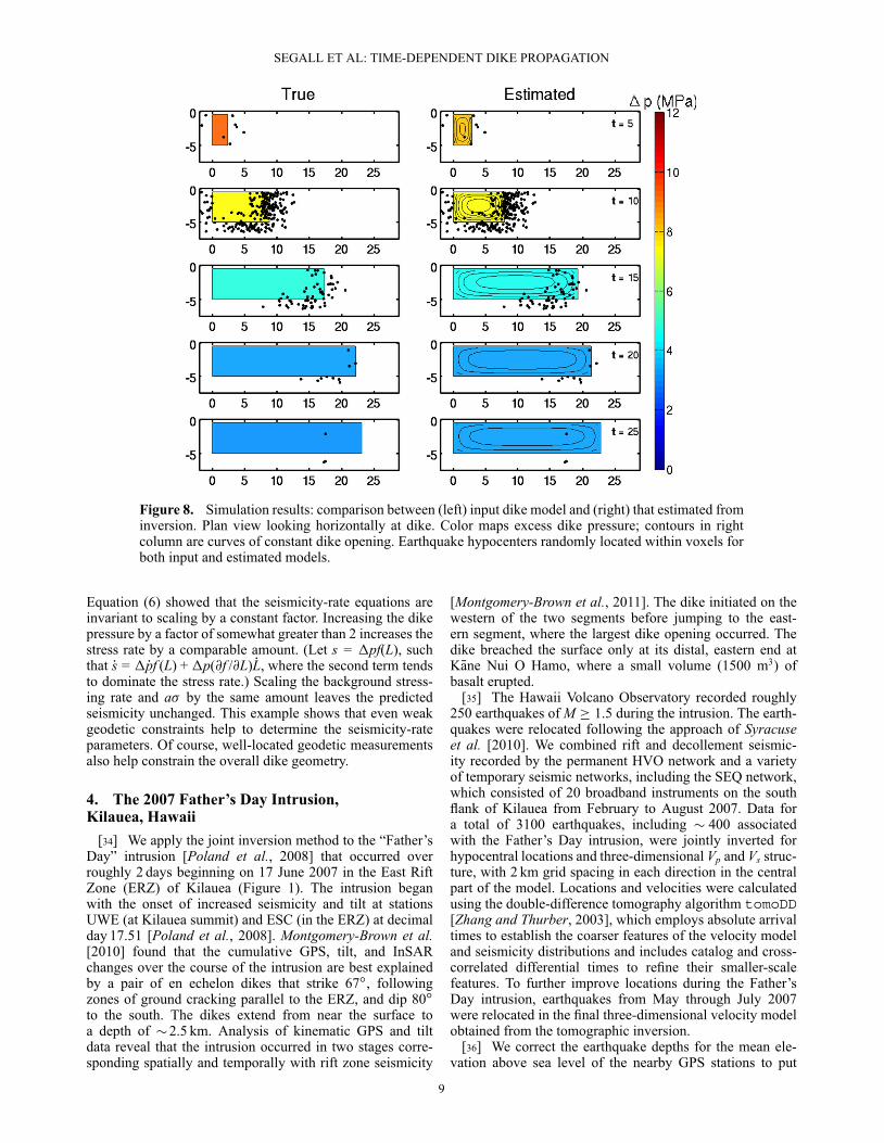
Figure 8. Simulation results: comparison between (left) input dike model and (right) that estimated frominversion. Plan view looking horizontally at dike. Color maps excess dike pressure; contours in rightcolumn are curves of constant dike opening. Earthquake hypocenters randomly located within voxels forboth input and estimated models.

Equation (6) showed that the seismicity-rate equations areinvariant to scaling by a constant factor. Increasing the dikepressure by a factor of somewhat greater than 2 increases thestress rate by a comparable amount. (Let s = �pf(L), suchthat Ps = �Ppf (L) +�p(@f /@L) PL, where the second term tendsto dominate the stress rate.) Scaling the background stress-ing rate and a� by the same amount leaves the predictedseismicity unchanged. This example shows that even weakgeodetic constraints help to determine the seismicity-rateparameters. Of course, well-located geodetic measurementsalso help constrain the overall dike geometry.

4. The 2007 Father’s Day Intrusion,Kilauea, Hawaii

[34] We apply the joint inversion method to the “Father’sDay” intrusion [Poland et al., 2008] that occurred overroughly 2 days beginning on 17 June 2007 in the East RiftZone (ERZ) of Kilauea (Figure 1). The intrusion beganwith the onset of increased seismicity and tilt at stationsUWE (at Kilauea summit) and ESC (in the ERZ) at decimalday 17.51 [Poland et al., 2008]. Montgomery-Brown et al.[2010] found that the cumulative GPS, tilt, and InSARchanges over the course of the intrusion are best explainedby a pair of en echelon dikes that strike 67ı, followingzones of ground cracking parallel to the ERZ, and dip 80ıto the south. The dikes extend from near the surface toa depth of �2.5 km. Analysis of kinematic GPS and tiltdata reveal that the intrusion occurred in two stages corre-sponding spatially and temporally with rift zone seismicity

[Montgomery-Brown et al., 2011]. The dike initiated on thewestern of the two segments before jumping to the east-ern segment, where the largest dike opening occurred. Thedike breached the surface only at its distal, eastern end atKane Nui O Hamo, where a small volume (1500 m3) ofbasalt erupted.

[35] The Hawaii Volcano Observatory recorded roughly250 earthquakes of M � 1.5 during the intrusion. The earth-quakes were relocated following the approach of Syracuseet al. [2010]. We combined rift and decollement seismic-ity recorded by the permanent HVO network and a varietyof temporary seismic networks, including the SEQ network,which consisted of 20 broadband instruments on the southflank of Kilauea from February to August 2007. Data fora total of 3100 earthquakes, including � 400 associatedwith the Father’s Day intrusion, were jointly inverted forhypocentral locations and three-dimensional Vp and Vs struc-ture, with 2 km grid spacing in each direction in the centralpart of the model. Locations and velocities were calculatedusing the double-difference tomography algorithm tomoDD[Zhang and Thurber, 2003], which employs absolute arrivaltimes to establish the coarser features of the velocity modeland seismicity distributions and includes catalog and cross-correlated differential times to refine their smaller-scalefeatures. To further improve locations during the Father’sDay intrusion, earthquakes from May through July 2007were relocated in the final three-dimensional velocity modelobtained from the tomographic inversion.

[36] We correct the earthquake depths for the mean ele-vation above sea level of the nearby GPS stations to put

9


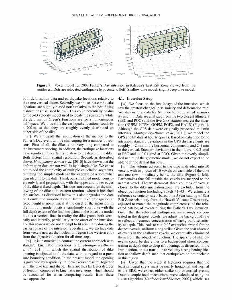
Figure 9. Voxel model for 2007 Father’s Day intrusion in Kilauea’s East Rift Zone viewed from thesouthwest. Dots are relocated earthquake hypocenters. (left) Shallow dike model; (right) deep dike model.

both deformation data and earthquake locations relative tothe same vertical datum. Secondly, we notice that earthquakelocations are slightly biased north relative to the best fittingdislocation (discussed below). This could potentially be dueto the 3-D velocity model used to locate the seismicity whilethe deformation Green’s functions are for a homogeneoushalf-space. We thus shift the earthquake locations south by� 700 m, so that they are roughly evenly distributed oneither side of the dike.

[37] We anticipate that application of the method to theFather’s Day event will be challenging for a number of rea-sons. First of all, the dike is not very long compared tothe instrument spacing. In addition, the earthquake locationshave significant uncertainty relative to the depth of the dike.Both factors limit spatial resolution. Second, as describedabove, Montgomery-Brown et al. [2010] have shown that thedeformation data are not well fit by a single dike. We chosenot to add the complexity of multiple en echelon segments,retaining the simpler model at the expense of a somewhatdegraded fit to the data. Third, our simplified model consid-ers only lateral propagation, with the upper and lower edgesof the dike at fixed depth. This does not account for the shal-lowing of the dike at its eastern terminus where it breachedthe surface; as discussed below this also degrades the datafit. Fourth, the simplification of lateral dike propagation atfixed height is nonphysical at the onset of the intrusion. Inthe limit this model posits a vanishingly short dike with thefull depth extent of the final intrusion; at the onset the modeldike is a vertical line. In reality the dike grows both verti-cally and laterally, particularly at the onset of the intrusion.For this reason we do not attempt to fit seismicity during theearliest phase of the intrusion. Specifically, we exclude datafrom voxels nearest the nucleation region (the western end)from the objective function for all time steps.

[38] It is instructive to contrast the current approach withstandard kinematic inversions [e.g, Montgomery-Brownet al., 2011], in which the spatial distribution of dikeopening is adjusted to fit the data, without regard to a pres-sure boundary condition. In the present model the openingis governed by a spatially uniform excess pressure, togetherwith the dike size and shape. There are thus far fewer degreesof freedom compared to kinematic inversions, which shouldbe accounted for when comparing results from thesetwo approaches.

4.1. Inversion Setup[39] We focus on the first 2 days of the intrusion, which

saw the greatest changes in seismicity and deformation rate.We also include data for 6 h prior to the onset of seismic-ity and tilt. Data are analyzed from the two closest tiltmeters(ESC and POO) and the five GPS stations nearest the intru-sion (NUPM, KTPM, GOPM, PGF2, and HALR) (Figure 1).Although the GPS data were originally processed at 4 minintervals [Montgomery-Brown et al., 2011], we model theGPS and tilt data at hourly epochs. Based on data prior to theintrusion, standard deviations in the GPS displacements areroughly 1–2 mm in the horizontal components and 2–3 mmin the vertical. Standard deviations in the tilt are � 0.2radat ESC and � 0.03rad at POO. Given the overly simpli-fied nature of the geometric model, we do not expect to beable to fit the data at this level.

[40] The volume adjacent to the dike is divided into 50voxels, with two rows of 10 voxels on each side of the dikeand one row immediately below the dike (Figure 9, left).Earthquakes that fall outside the voxels are mapped to thenearest voxel. The westernmost three columns of voxels,closest to the dike nucleation zone, are excluded from theobjective function (including voxels 41–43). We estimate areference seismicity rate r based on a 5 year catalog of EastRift Zone seismicity from the Hawaii Volcano Observatory,adjusted to match the magnitude completeness of the relo-cated catalog of events during the Father’s Day intrusion.Given that the relocated earthquakes are strongly concen-trated in the deepest voxels, we adjust the background rateto reflect a presumed concentration of background seismic-ity at depth. This leads to r ' 0.02 events/hour/voxel for thedeepest voxels, uniform along strike. Given the near absenceof events in the shallower voxels, we eventually eliminatedthem from the objective function. The sparsity of shallowevents could be due either to a background stress concen-tration at depth due to deep rift opening, as discussed in theIntroduction, or to a transition to velocity strengthening fric-tion at shallow depth such that earthquakes do not nucleatein this region.

[41] Given that the regional tectonics requires that theleast principal stress must be nearly horizontal and normalto the ERZ, we expect either strike-slip or normal events.Double-couple focal mechanisms were calculated using theHASH algorithm [Hardebeck and Shearer, 2002], which uses

10


-155.23 -155.22 -155.21 -155.219.36

19.37

2.4 2.6

depth (km)

0.5 km

Figure 10. Focal mechanisms for better constrained earthquakes during the Father’s Day intrusion.The outlined mechanism is for a M 2.2 earthquake on 26 May 2007. The others occurred during theFather’s Day event. Focal mechanisms are lower-hemisphere projections showing polarities (greencircle = positive first motion, compressional; black cross = negative first motion, dilatational).

P wave first motions and model uncertainties to calculatethe most likely solution for each earthquake. Takeoff anglesand azimuths were calculated using the hypocenters andthree-dimensional Vp model described previously. (Discus-sion of reversed polarities at several HVO stations appearsin Appendix C.) The nine highest-quality focal mechanismsare shown in Figure 10. The outlined mechanism is for aM 2.2 earthquake on 26 May 2007, while the remaining eightare for M 2.2–2.6 earthquakes within a 5 h period on 17 June2007. Consistent with expectations, the focal mechanismspredominantly show oblique right-lateral motion along near-vertical slip planes oriented at N46ıE. The general similaritybetween the focal mechanism for the May and 17 June earth-quakes indicates that the absolute stress state did not changesubstantially during the intrusion.

[42] We thus compute the stress changes on (near) verticalplanes oriented at ˙30ı from the dike plane. The coeffi-cient of friction is assumed to be 0.6 and the background

normal stress and pore-pressure lithostatic and hydrostatic,respectively. This does not account for the extensional stressregime within Kilauea’s ERZ. Thus, estimates of the frictionparameter a will include a contribution from the deviationof the effective normal stress from the assumed backgroundstate (see section 5).

[43] We assume an overall dike geometry consistentwith kinematic models of the intrusion [Montgomery-Brownet al., 2010, 2011] but adjusted to account for thesingle dike segment with fixed top and bottom depth. Thisoverly simplified geometric model is incapable of fittingboth the tilt at ESC and the GPS displacement at NUPM(Figure 11). We find that a reasonable compromise isachieved with a dike that strikes N73ıE, dips 85ı south, withheight (in the dip direction) of 2.4 km. Figure 11 illustratesthe difficulty in fitting the cumulative deformation over the2 days of the intrusion with the restricted geometric model,varying only the depth to the top of the dike. Recall that the

5 10 15 20

−5

0

5

10

A) Top Depth: 600

Distance [km]

B) Top Depth: 350

Distance [km]

C) Top Depth: 200

Distance [km]5 10 15 20 5 10 15 20

Figure 11. Influence of depth to the top of the dike on cumulative displacement and tilt (dashed).Observed (black with error ellipses inflated by a factor of 10) and predicted (red) vectors. Dike is subjectto spatially uniform excess pressure of 8.5 MPa. Top of dike at (a) 600 m, (b) 350 m, and (c) 200 m.

11


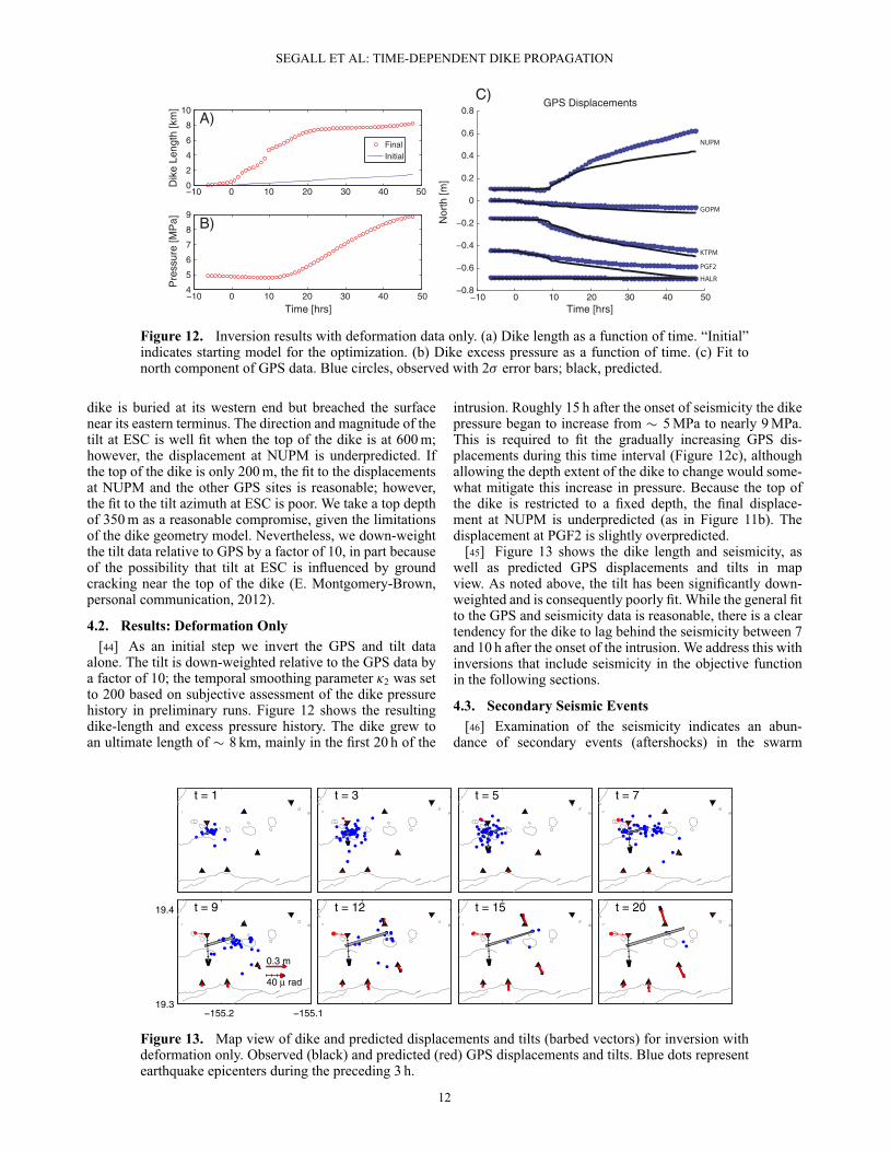
Figure 12. Inversion results with deformation data only. (a) Dike length as a function of time. “Initial”indicates starting model for the optimization. (b) Dike excess pressure as a function of time. (c) Fit tonorth component of GPS data. Blue circles, observed with 2� error bars; black, predicted.

dike is buried at its western end but breached the surfacenear its eastern terminus. The direction and magnitude of thetilt at ESC is well fit when the top of the dike is at 600 m;however, the displacement at NUPM is underpredicted. Ifthe top of the dike is only 200 m, the fit to the displacementsat NUPM and the other GPS sites is reasonable; however,the fit to the tilt azimuth at ESC is poor. We take a top depthof 350 m as a reasonable compromise, given the limitationsof the dike geometry model. Nevertheless, we down-weightthe tilt data relative to GPS by a factor of 10, in part becauseof the possibility that tilt at ESC is influenced by groundcracking near the top of the dike (E. Montgomery-Brown,personal communication, 2012).

4.2. Results: Deformation Only[44] As an initial step we invert the GPS and tilt data

alone. The tilt is down-weighted relative to the GPS data bya factor of 10; the temporal smoothing parameter �2 was setto 200 based on subjective assessment of the dike pressurehistory in preliminary runs. Figure 12 shows the resultingdike-length and excess pressure history. The dike grew toan ultimate length of � 8 km, mainly in the first 20 h of the

intrusion. Roughly 15 h after the onset of seismicity the dikepressure began to increase from � 5 MPa to nearly 9 MPa.This is required to fit the gradually increasing GPS dis-placements during this time interval (Figure 12c), althoughallowing the depth extent of the dike to change would some-what mitigate this increase in pressure. Because the top ofthe dike is restricted to a fixed depth, the final displace-ment at NUPM is underpredicted (as in Figure 11b). Thedisplacement at PGF2 is slightly overpredicted.

[45] Figure 13 shows the dike length and seismicity, aswell as predicted GPS displacements and tilts in mapview. As noted above, the tilt has been significantly down-weighted and is consequently poorly fit. While the general fitto the GPS and seismicity data is reasonable, there is a cleartendency for the dike to lag behind the seismicity between 7and 10 h after the onset of the intrusion. We address this withinversions that include seismicity in the objective functionin the following sections.

4.3. Secondary Seismic Events[46] Examination of the seismicity indicates an abun-

dance of secondary events (aftershocks) in the swarm

t = 1 t = 3 t = 5 t = 7

−155.2 −155.119.3

19.4

0.3 m

40 µ rad

t = 9 t = 12 t = 15 t = 20

Figure 13. Map view of dike and predicted displacements and tilts (barbed vectors) for inversion withdeformation only. Observed (black) and predicted (red) GPS displacements and tilts. Blue dots representearthquake epicenters during the preceding 3 h.

12


A) B)

C)

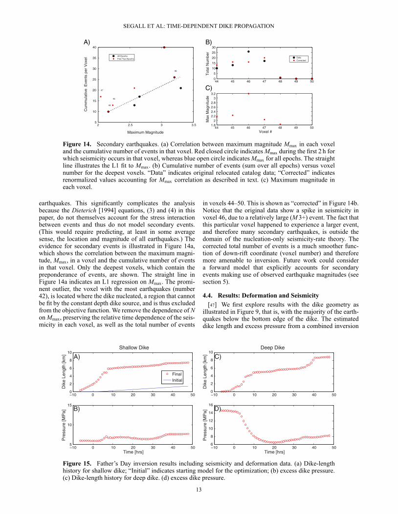
Figure 14. Secondary earthquakes. (a) Correlation between maximum magnitude Mmax in each voxeland the cumulative number of events in that voxel. Red closed circle indicates Mmax during the first 2 h forwhich seismicity occurs in that voxel, whereas blue open circle indicates Mmax for all epochs. The straightline illustrates the L1 fit to Mmax. (b) Cumulative number of events (sum over all epochs) versus voxelnumber for the deepest voxels. “Data” indicates original relocated catalog data; “Corrected” indicatesrenormalized values accounting for Mmax correlation as described in text. (c) Maximum magnitude ineach voxel.

earthquakes. This significantly complicates the analysisbecause the Dieterich [1994] equations, (3) and (4) in thispaper, do not themselves account for the stress interactionbetween events and thus do not model secondary events.(This would require predicting, at least in some averagesense, the location and magnitude of all earthquakes.) Theevidence for secondary events is illustrated in Figure 14a,which shows the correlation between the maximum magni-tude, Mmax, in a voxel and the cumulative number of eventsin that voxel. Only the deepest voxels, which contain thepreponderance of events, are shown. The straight line inFigure 14a indicates an L1 regression on Mmax. The promi-nent outlier, the voxel with the most earthquakes (number42), is located where the dike nucleated, a region that cannotbe fit by the constant depth dike source, and is thus excludedfrom the objective function. We remove the dependence of Non Mmax, preserving the relative time dependence of the seis-micity in each voxel, as well as the total number of events

in voxels 44–50. This is shown as “corrected” in Figure 14b.Notice that the original data show a spike in seismicity invoxel 46, due to a relatively large (M 3+) event. The fact thatthis particular voxel happened to experience a larger event,and therefore many secondary earthquakes, is outside thedomain of the nucleation-only seismicity-rate theory. Thecorrected total number of events is a much smoother func-tion of down-rift coordinate (voxel number) and thereforemore amenable to inversion. Future work could considera forward model that explicitly accounts for secondaryevents making use of observed earthquake magnitudes (seesection 5).

4.4. Results: Deformation and Seismicity[47] We first explore results with the dike geometry as

illustrated in Figure 9, that is, with the majority of the earth-quakes below the bottom edge of the dike. The estimateddike length and excess pressure from a combined inversion

−10 0 10 20 30 40 500

2

4

6

8

10

Dik

e Le

ngth

[km

] A)

FinalInitial

−10 0 10 20 30 40 505

10

15

Pre

ssur

e [M

Pa]

Time [hrs]

B)

−10 0 10 20 30 40 500

2

4

6

8

10

Dik

e Le

ngth

[km

] C)

−10 0 10 20 30 40 506

8

10

12

14

16

Pre

ssur

e [M

Pa]

Time [hrs]

D)

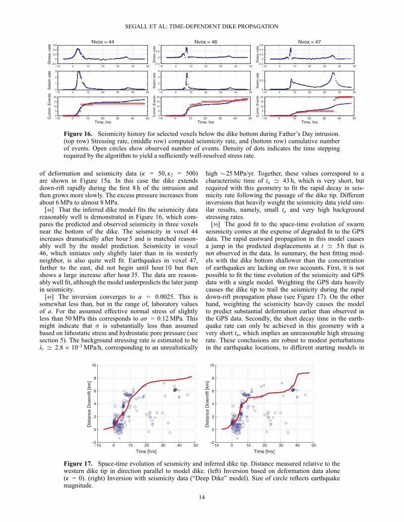
Shallow Dike Deep Dike

Figure 15. Father’s Day inversion results including seismicity and deformation data. (a) Dike-lengthhistory for shallow dike; “Initial” indicates starting model for the optimization; (b) excess dike pressure.(c) Dike-length history for deep dike. (d) excess dike pressure.

13


Figure 16. Seismicity history for selected voxels below the dike bottom during Father’s Day intrusion.(top row) Stressing rate, (middle row) computed seismicity rate, and (bottom row) cumulative numberof events. Open circles show observed number of events. Density of dots indicates the time steppingrequired by the algorithm to yield a sufficiently well-resolved stress rate.

of deformation and seismicity data (� = 50, �2 = 500)are shown in Figure 15a. In this case the dike extendsdown-rift rapidly during the first 8 h of the intrusion andthen grows more slowly. The excess pressure increases fromabout 6 MPa to almost 8 MPa.

[48] That the inferred dike model fits the seismicity datareasonably well is demonstrated in Figure 16, which com-pares the predicted and observed seismicity in three voxelsnear the bottom of the dike. The seismicity in voxel 44increases dramatically after hour 5 and is matched reason-ably well by the model prediction. Seismicity in voxel46, which initiates only slightly later than in its westerlyneighbor, is also quite well fit. Earthquakes in voxel 47,farther to the east, did not begin until hour 10 but thenshows a large increase after hour 35. The data are reason-ably well fit, although the model underpredicts the later jumpin seismicity.

[49] The inversion converges to a = 0.0025. This issomewhat less than, but in the range of, laboratory valuesof a. For the assumed effective normal stress of slightlyless than 50 MPa this corresponds to a� = 0.12 MPa. Thismight indicate that � is substantially less than assumedbased on lithostatic stress and hydrostatic pore pressure (seesection 5). The background stressing rate is estimated to bePsr ' 2.8 � 10–3 MPa/h, corresponding to an unrealistically

high �25 MPa/yr. Together, these values correspond to acharacteristic time of ta ' 43 h, which is very short, butrequired with this geometry to fit the rapid decay in seis-micity rate following the passage of the dike tip. Differentinversions that heavily weight the seismicity data yield sim-ilar results, namely, small ta and very high backgroundstressing rates.

[50] The good fit to the space-time evolution of swarmseismicity comes at the expense of degraded fit to the GPSdata. The rapid eastward propagation in this model causesa jump in the predicted displacements at t ' 5 h that isnot observed in the data. In summary, the best fitting mod-els with the dike bottom shallower than the concentrationof earthquakes are lacking on two accounts. First, it is notpossible to fit the time evolution of the seismicity and GPSdata with a single model. Weighting the GPS data heavilycauses the dike tip to trail the seismicity during the rapiddown-rift propagation phase (see Figure 17). On the otherhand, weighting the seismicity heavily causes the modelto predict substantial deformation earlier than observed inthe GPS data. Secondly, the short decay time in the earth-quake rate can only be achieved in this geometry with avery short ta, which implies an unreasonable high stressingrate. These conclusions are robust to modest perturbationsin the earthquake locations, to different starting models in

−10 0 10 20 30 40 50−2

0

2

4

6

8

10

Time [hrs]

Dis

tanc

e D

ownr

ift [k

m]

−10 0 10 20 30 40 50−2

0

2

4

6

8

10

Time [hrs]

Dis

tanc

e D

ownr

ift [k

m]

Figure 17. Space-time evolution of seismicity and inferred dike tip. Distance measured relative to thewestern dike tip in direction parallel to model dike. (left) Inversion based on deformation data alone(� = 0). (right) Inversion with seismicity data (“Deep Dike” model). Size of circle reflects earthquakemagnitude.

14


−10 0 10 20 30 40 50−6−4−2

02

Str

ess−

rate

Nvox = 5

−10 0 10 20 30 40 500

2

4

6

Sei

sm r

ate

−10 0 10 20 30 40 5005

101520

Cum

m. E

vent

s

Time, hrs

−10 0 10 20 30 40 50−15−10−505

Str

ess−

rate

Nvox = 7

−10 0 10 20 30 40 500

5

10

Sei

sm r

ate

−10 0 10 20 30 40 500

5

10

Cum

m. E

vent

s

Time, hrs

−10 0 10 20 30 40 50−2−1012

Str

ess−

rate

Nvox = 11

−10 0 10 20 30 40 500

0.51

1.52

Sei

sm r

ate

−10 0 10 20 30 40 500

5

10

Cum

m. E

vent

s

Time, hrs

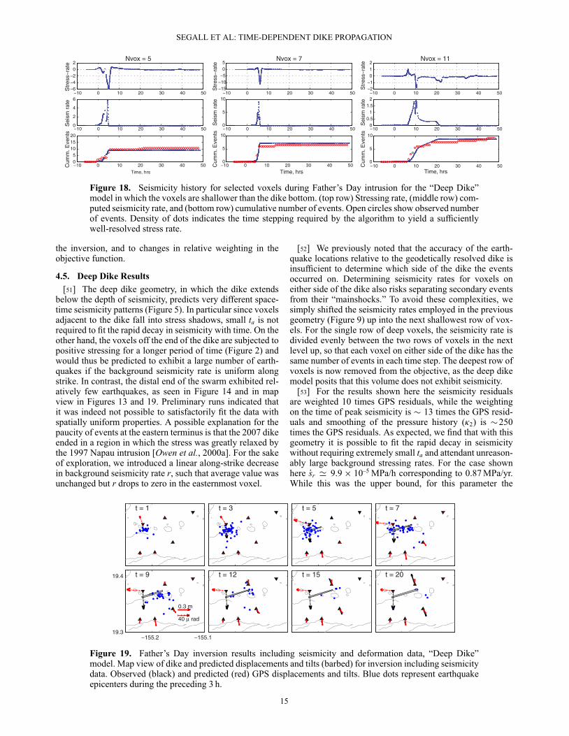
Figure 18. Seismicity history for selected voxels during Father’s Day intrusion for the “Deep Dike”model in which the voxels are shallower than the dike bottom. (top row) Stressing rate, (middle row) com-puted seismicity rate, and (bottom row) cumulative number of events. Open circles show observed numberof events. Density of dots indicates the time stepping required by the algorithm to yield a sufficientlywell-resolved stress rate.

the inversion, and to changes in relative weighting in theobjective function.

4.5. Deep Dike Results[51] The deep dike geometry, in which the dike extends

below the depth of seismicity, predicts very different space-time seismicity patterns (Figure 5). In particular since voxelsadjacent to the dike fall into stress shadows, small ta is notrequired to fit the rapid decay in seismicity with time. On theother hand, the voxels off the end of the dike are subjected topositive stressing for a longer period of time (Figure 2) andwould thus be predicted to exhibit a large number of earth-quakes if the background seismicity rate is uniform alongstrike. In contrast, the distal end of the swarm exhibited rel-atively few earthquakes, as seen in Figure 14 and in mapview in Figures 13 and 19. Preliminary runs indicated thatit was indeed not possible to satisfactorily fit the data withspatially uniform properties. A possible explanation for thepaucity of events at the eastern terminus is that the 2007 dikeended in a region in which the stress was greatly relaxed bythe 1997 Napau intrusion [Owen et al., 2000a]. For the sakeof exploration, we introduced a linear along-strike decreasein background seismicity rate r, such that average value wasunchanged but r drops to zero in the easternmost voxel.

[52] We previously noted that the accuracy of the earth-quake locations relative to the geodetically resolved dike isinsufficient to determine which side of the dike the eventsoccurred on. Determining seismicity rates for voxels oneither side of the dike also risks separating secondary eventsfrom their “mainshocks.” To avoid these complexities, wesimply shifted the seismicity rates employed in the previousgeometry (Figure 9) up into the next shallowest row of vox-els. For the single row of deep voxels, the seismicity rate isdivided evenly between the two rows of voxels in the nextlevel up, so that each voxel on either side of the dike has thesame number of events in each time step. The deepest row ofvoxels is now removed from the objective, as the deep dikemodel posits that this volume does not exhibit seismicity.

[53] For the results shown here the seismicity residualsare weighted 10 times GPS residuals, while the weightingon the time of peak seismicity is � 13 times the GPS resid-uals and smoothing of the pressure history (�2) is �250times the GPS residuals. As expected, we find that with thisgeometry it is possible to fit the rapid decay in seismicitywithout requiring extremely small ta and attendant unreason-ably large background stressing rates. For the case shownhere Psr ' 9.9 � 10–5 MPa/h corresponding to 0.87 MPa/yr.While this was the upper bound, for this parameter the

t = 1 t = 3 t = 5 t = 7

−155.2 −155.119.3

19.4

0.3 m

40 µ rad

t = 9 t = 12 t = 15 t = 20

Figure 19. Father’s Day inversion results including seismicity and deformation data, “Deep Dike”model. Map view of dike and predicted displacements and tilts (barbed) for inversion including seismicitydata. Observed (black) and predicted (red) GPS displacements and tilts. Blue dots represent earthquakeepicenters during the preceding 3 h.

15


0.8

0.6

0.4

0.8

0

-0.2

-0.4

-0.6

-0.8-10 0 10 3020 40 50

Nor

th [m

]

Time [hrs]

GPS Displacements

NUPM

GOPM

KTPM

PGF2

HALR

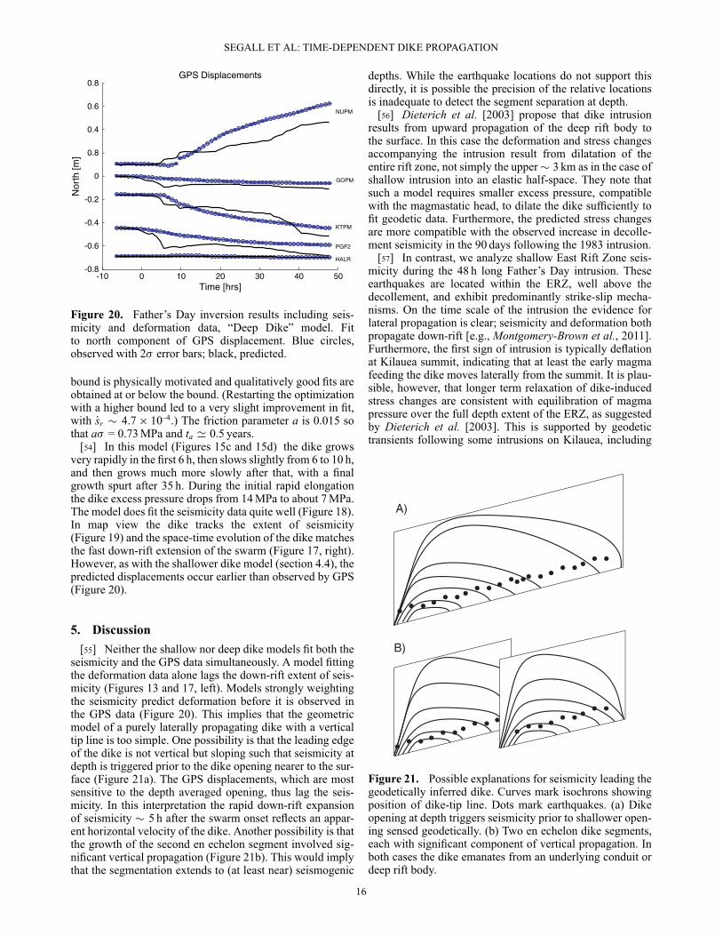
Figure 20. Father’s Day inversion results including seis-micity and deformation data, “Deep Dike” model. Fitto north component of GPS displacement. Blue circles,observed with 2� error bars; black, predicted.

bound is physically motivated and qualitatively good fits areobtained at or below the bound. (Restarting the optimizationwith a higher bound led to a very slight improvement in fit,with Psr � 4.7 � 10–4.) The friction parameter a is 0.015 sothat a� = 0.73 MPa and ta ' 0.5 years.

[54] In this model (Figures 15c and 15d) the dike growsvery rapidly in the first 6 h, then slows slightly from 6 to 10 h,and then grows much more slowly after that, with a finalgrowth spurt after 35 h. During the initial rapid elongationthe dike excess pressure drops from 14 MPa to about 7 MPa.The model does fit the seismicity data quite well (Figure 18).In map view the dike tracks the extent of seismicity(Figure 19) and the space-time evolution of the dike matchesthe fast down-rift extension of the swarm (Figure 17, right).However, as with the shallower dike model (section 4.4), thepredicted displacements occur earlier than observed by GPS(Figure 20).

5. Discussion[55] Neither the shallow nor deep dike models fit both the

seismicity and the GPS data simultaneously. A model fittingthe deformation data alone lags the down-rift extent of seis-micity (Figures 13 and 17, left). Models strongly weightingthe seismicity predict deformation before it is observed inthe GPS data (Figure 20). This implies that the geometricmodel of a purely laterally propagating dike with a verticaltip line is too simple. One possibility is that the leading edgeof the dike is not vertical but sloping such that seismicity atdepth is triggered prior to the dike opening nearer to the sur-face (Figure 21a). The GPS displacements, which are mostsensitive to the depth averaged opening, thus lag the seis-micity. In this interpretation the rapid down-rift expansionof seismicity � 5 h after the swarm onset reflects an appar-ent horizontal velocity of the dike. Another possibility is thatthe growth of the second en echelon segment involved sig-nificant vertical propagation (Figure 21b). This would implythat the segmentation extends to (at least near) seismogenic

depths. While the earthquake locations do not support thisdirectly, it is possible the precision of the relative locationsis inadequate to detect the segment separation at depth.

[56] Dieterich et al. [2003] propose that dike intrusionresults from upward propagation of the deep rift body tothe surface. In this case the deformation and stress changesaccompanying the intrusion result from dilatation of theentire rift zone, not simply the upper� 3 km as in the case ofshallow intrusion into an elastic half-space. They note thatsuch a model requires smaller excess pressure, compatiblewith the magmastatic head, to dilate the dike sufficiently tofit geodetic data. Furthermore, the predicted stress changesare more compatible with the observed increase in decolle-ment seismicity in the 90 days following the 1983 intrusion.

[57] In contrast, we analyze shallow East Rift Zone seis-micity during the 48 h long Father’s Day intrusion. Theseearthquakes are located within the ERZ, well above thedecollement, and exhibit predominantly strike-slip mecha-nisms. On the time scale of the intrusion the evidence forlateral propagation is clear; seismicity and deformation bothpropagate down-rift [e.g., Montgomery-Brown et al., 2011].Furthermore, the first sign of intrusion is typically deflationat Kilauea summit, indicating that at least the early magmafeeding the dike moves laterally from the summit. It is plau-sible, however, that longer term relaxation of dike-inducedstress changes are consistent with equilibration of magmapressure over the full depth extent of the ERZ, as suggestedby Dieterich et al. [2003]. This is supported by geodetictransients following some intrusions on Kilauea, including

A)

B)

Figure 21. Possible explanations for seismicity leading thegeodetically inferred dike. Curves mark isochrons showingposition of dike-tip line. Dots mark earthquakes. (a) Dikeopening at depth triggers seismicity prior to shallower open-ing sensed geodetically. (b) Two en echelon dike segments,each with significant component of vertical propagation. Inboth cases the dike emanates from an underlying conduit ordeep rift body.

16


the1997 Napau eruption, that are best explained by delayedrift opening below a shallow dike intrusion [Desmarais andSegall, 2007].

[58] If the intrusion-induced seismicity is dominantly trig-gered by the laterally propagating dike tip, then the localizeddepth extent of earthquakes is controlled by the depth depen-dence of the background stressing generated by continuousdeep rift opening. A pronounced stress concentration nearthe top of the deep rift body is consistent with the narrowdepth extent of background seismicity [Gillard et al., 1996].This stress concentration may also control where individualdikes nucleate. Dikes could also nucleate from the con-duit feeding the Pu’u ’O’o vent—it is presently unknownwhether the conduit coincides with the top of the deep riftbody. In either case, the preexisting conduit provides a path-way for magma from the summit magma reservoir into thedike. Subsidence of the crater floor at Pu’u ’O’o during theeruption [Poland et al., 2008; Montgomery-Brown et al.,2010] also indicates that magma flowed from Pu’u ’O’o intothe dike. During intrusions the stress concentration at theleading dike edge adds to the highly localized backgroundstress. This suggests that seismicity occurs at the bottom ofthe brittle region, where the background stressing is high-est. Since seismicity rate during intrusions is proportionalto the background rate (see equation (3)), it is expected thatbackground and swarm earthquakes are concentrated at thesame depth.

[59] Yet another possible explanation for the rapid decayin seismicity during the intrusion would be that the seis-micity is originally located beneath the dike (“shallow dikemodel”), but the dike rapidly deepens dropping the seismi-cally active volume into a stress shadow. This seems lesslikely if dikes nucleate in the stress concentration at the topof the deep rift body, although this effect could occur locallyalong strike as the dike propagates down-rift.

[60] The model fit to deformation data alone results indike pressure increasing with time (Figure 12), whereas thedeep dike model weighted to fit seismicity exhibits decreas-ing dike pressure (Figure 15). The latter is more in accordwith expectation, since dike growth increases the net volumeof the magmatic system and without addition of new magmamust result in a pressure drop [e.g., Segall et al., 2001].

[61] We have ignored thermal and thermo-poro-elasticstressing, as this is unlikely to be important on the timescale of dike propagation [Rubin and Gillard, 1998]. A diketraverses a region of spatial extent D in time D/v. For prop-agation speeds v of order 0.1 km/h or 3 cm/s and earthquakesources on the scale of 300 m, this corresponds to times oforder 104 s. Thermal diffusivity of rock is of the order ofc = 10–6m2/s, which leads to thermal penetration distancesL =p

ct of order 10–1 m. Similarly, pore-pressure increasesdue to heating are only significant when the hydraulic diffu-sivity is small, and in these cases the penetration distanceson the time scale of dike propagation are insignificant.

[62] The analysis also neglected the presence of a dike-tipcavity which is filled with either pore fluids from the sur-rounding rock or exsolved fluids from the magma. Thesefluids exist at �p < 0 and permit the dike to close smoothlywithout stress singularity [Rubin, 1995]. The stresses com-puted from a uniformly pressurized crack are only accurateif the dike-tip cavity is small relative to the distance of theearthquakes from the dike. The length scale of the dike-tip

region depends on the degree of under pressure within thetip, which is not well known. Depending on the proxim-ity of earthquakes to the dike, neglecting the dike-tip cavitymay result in overestimating the dike-induced stress change.This is mitigated to some extent by the fact that we com-pute the stress at voxel centers some distance from the dikeplane. Biases in the computed stress are likely to bias thebackground stressing rate and friction parameter a.

[63] The depth dependence of excess dike pressure alsovaries due to crustal density variations and depth dependentrheology. It is believed that bladelike dikes are trapped byzones of positive excess pressure, such that �p decreasestoward both the top and bottom of the dike. (These dike-trapping stresses are associated with what is commonlyreferred to as the “level of neutral buoyancy” [Rubin, 1995].)We examined the effect of depth-dependent pressure on thetime-dependent inversion assuming a bilinear distribution ofexcess dike pressure with depth, �p(z) = p0 – p0|z – zc|,where p0 is the pressure at the dike center (depth zc) andp0 is the vertical pressure gradient. Choosing the gradient inpressure such that the stress intensity factors vanish at theupper and lower edges (according to a plane-strain calcula-tion) requires p0 = p0/h, where h is dike height [Fialkoand Rubin, 1999, equation (3)]. At the dike top and bot-tom the excess pressure is negative (under pressure), �p =–p0( – 2)/2.

[64] With the bilinear pressure distribution the averageexcess pressure is reduced by a factor of 1.14/4 relative tothe uniformly pressurized dike. Thus, either the peak pres-sure has to be increased by a factor of � 4 relative to theuniform case (for the same dike height) or the shear modulushas to be reduced by a factor of � 4 to achieve an equiva-lent fit to the GPS displacements. GPS stations close to therift zone are sensitive to the reduced shallow opening withthe bilinear pressure distribution. We found that bringing thedike top to 100 m below the surface provides a reasonable fitto the data at NUPM.

[65] The rate of stressing computed at a voxel center canbe much more than a factor of 4 less than computed inthe uniform pressure case, depending on distance from thedike edge to the voxel center. (The stress, unlike displace-ment, does not scale with shear modulus given a pressureboundary condition.) With nonuniform pressure the stressdistribution changes (in particular, the stress shadow is elim-inated immediately above the dike bottom), so the stress-ratehistory is not simply a scaled version of the uniform pres-sure case. However, if the earthquakes are located below thedike bottom, the stress histories for the two pressure distri-butions are close to scaled versions of one another. In thiscase, scaling Psr and a� by the ratio of the bilinear to uniformstressing rates should leave the predicted seismicity raterelatively unchanged.

[66] We tested this with the “shallow dike” model, takingthe solution described in the paper as a starting model butchanging the pressure distribution to be bilinear, reducingthe shear modulus by a factor of 4, and reducing the previousestimates of Psr and a� by factors of 10. The resulting dikemodel is qualitatively similar to previous estimates, althoughsomewhat different in detail. The peak excess pressure (atthe dike center) drops from � 7.5 MPa to � 5 MPa as thedike evolves. The predicted displacements lead the observa-tions, as observed in other such models when the seismicity

17


data is heavily weighted in the objective. The backgroundstressing rate is decreased to on the order of 2 MPa/yr; how-ever, a� is also reduced in order to maintain ta to � 8 days.Starting with an initial model much farther from the finalestimate resulted in a similar but not identical result. Forthe deep dike model the stress driving strike-slip faultingadjacent to the dike depends strongly on depth. Future inver-sions will need to average over depth within voxels (ratherthan evaluate only at voxel centers) to properly comparepredictions with observed seismicity.

[67] The deep dike model posits that the dike bottomextended at least somewhat below the brittle-ductile tran-sition for earthquakes. This suggests that dike-trappingstresses and hence the “level of neutral buoyancy” isstrongly influenced by the brittle-ductile transition in combi-nation with south flank motion, as opposed to simply densitystratification. This inference is consistent with the observa-tion that the 2–3 km depth of diking [e.g., Owen et al., 2000a;Cervelli et al., 2002; Montgomery-Brown et al., 2010] isindistinguishable from the top of the deep rift body [e.g.,Delaney et al., 1990; Owen et al., 2000b].

[68] Estimates of the friction parameter a are conditionalon the effective normal stress acting on the earthquakesources � being lithostatic less hydrostatic pore pressure. Inaddition to uncertainties in pore pressure, the total stress act-ing on strike-slip faults is likely to be less than lithostatic.Assume that the intermediate principal stress is vertical(lithostatic). The minimum compressive stress (rift normal)can be no less than some fraction � (roughly 0.3) of the ver-tical stress without normal faulting occurring within the riftzone [Segall et al., 2001]. The oblique focal mechanismssuggest that the maximum compression is not much greaterthan the vertical stress. Taking this limit, the ratio of averagehorizontal stress to vertical stress is (1 + �)/2. From a Mohr’scircle construction, the ratio of � acting on faults at failureto the average horizontal stress is 1/(1 + f 2), where f is thefriction coefficient. Thus, the ratio of � to vertical stress is(1 + �)/2(1 + f 2), which for � � 0.3 and f � 0.6 is of theorder 0.5. This is almost certainly not the greatest source ofuncertainty in the estimates of a.

[69] The absence of source interactions in the Dieterich[1994] theory is a significant limitation in applying themodel to swarm sequences which contain secondary events.Attempts at declustering the earthquake catalog failedbecause they removed nearly all of the events. It is pos-sible that an appropriate declustering algorithm would beuseful. Another option would be to include an ETAS-like[Ogata, 1998] term in the forward model, perhaps allow-ing the largest events in the sequence to produce a cascadeof secondary events. Of course a better solution would beto develop a physical model that predicts secondary events;however, this requires predicting the ultimate size of anearthquake once initiated, which is currently out of reach ofanalytical models.

6. Conclusion[70] We have developed methods for the forward mod-

eling and inversion of seismicity and deformation accom-panying dike intrusion, assuming volcano-tectonic eventsresulting from shear failure of rock near the dike. For sim-plicity we currently model lateral propagation only and

estimate the dike length and overpressure at each time step.Forward models show that when seismicity is at intermediatedepth between the dike top and bottom, earthquakes initiatenear the leading edge of the dike, but seismicity cuts off asthe dike tip passes and the seismogenic volume falls into astress shadow. The crust off the dike ends, however, experi-ences more earthquakes as these volumes undergo positivestressing for a greater length of time. On the other hand, ifquakes occur above or below the dike, seismicity is predictedto continue at a decaying rate after the dike tip passes. Bothspace-time patterns have been observed in nature.

[71] We apply the inversion approach to the 2007 Father’sDay intrusion in Kilauea Volcano, Hawaii. Swarm seismic-ity during the intrusion propagated down-rift to the east, islocalized in a narrow depth range at � 3 km, comparableto geodetic estimates of the dike bottom, and decays rapidlywith time. We find that with lateral propagation and a verticaltip line it is difficult to fit both GPS data and the rapid down-rift jump in seismicity. This suggests significant verticalpropagation during the intrusion, such that the rapid down-rift expansion of the swarm reflects an apparent velocity ofdike propagation. One possibility is that each of the two enechelon dike segments inferred from steaming ground frac-tures and kinematic modeling of InSAR, GPS, and tilt dataextend to significant depth. Vertical propagation of the sec-ond segment could then account for the rapid down-rift jumpin seismicity.

[72] We explore both a “shallow” dike model, in whichthe seismicity is concentrated below the bottom edge of thedike, and a “deep dike” model, in which the dike extendsbelow the seismicity. In the context of the deep model, therapid decay in seismicity results from passage of the diketip and seismicity falling into a stress shadow. In contrast,in the shallow dike model the rapid decay in seismicityrate following the passage of the dike tip requires a veryshort aftershock decay time and hence an unrealisticallyhigh background stressing rate. The deep dike model thusseems more consistent with the observations. However, ifbackground stressing and seismicity rates are uniform alongstrike in Kilauea’s East Rift Zone, the deep dike model pre-dicts a strong concentration of seismicity at the eastern endof the intrusion, which is not observed. This apparent dis-crepancy could be explained if the 2007 dike ended in avolume of rock de-stressed by the 1999 Napau intrusionand eruption.

Appendix A: Omori Limit of Seismicity Equations[73] We consider the following case: start at background

stressing rate Psr and state �0 = 1/ Psr. Step 1, for a short periodof length �t, increase the stressing rate to Ps � Psr. Thismodels rapid stressing during the intrusion. Step 2, returnto stressing rate Psr. For step 1, equation (8), in the limitPsr/Ps� 1, reduces to

R1

r' exp

�–Ps�ta�

�= exp

�–�sa�

�. (A1)

At the same time, � evolves from (7) to

�1 '1Psr

exp�

–�sa�

�. (A2)

18


[74] For step 2, the state starts at �1 and again evolvesaccording to equation (8). This yields

Rr'

1(e–�s/a� – 1)e–t/ta + 1

. (A3)

The above is equivalent to Dieterich [1994] equation (12)when the stressing rate following the event returns to thebackground rate. For short times following the intrusion,t/ta � 1, including the leading order terms in a Taylor seriesexpansion of the exponential term, equation (A3) reduces to

Rr'

1e–�s/a� + t

ta

, (A4)

which is of the form of Omori’s law.

Appendix B: Implementation Details

B1. Forward Calculations[75] It is important to ensure that the piecewise linear

discretization of the stress is accurate. To that end if thestress rate in any voxel exceeds a predefined threshold, thetime step is divided into uniform length substeps. The dikelength L is linearly interpolated through the substeps, whilethe magma pressure history is estimated by cubic interpo-lation. The stress rate is computed from the derivative of acubic spline fit to the stress computed at the substeps. Test-ing showed that this resulted in a smooth stress-rate history.Examples can be seen in Figure 16.

[76] Care also needs to be given to equations (7) through(9) in cases where | Psk�tk/a� | � 1. Equation (7) in the limitof Psk�tk/a� � 0 can lead to overflow, corresponding to� ! 1 and R ! 0. This is not a problem for a sin-gle dike intrusion; however, it should be noted that once anoverflow condition occurs the seismicity rate can never benonzero, even if the stress rate at a later time becomes pos-itive. If Psk�tk/a� � 1 but �k–1 Psk is finite, then (9) and (10)lead to N ' rta ( Psk�tk/a� – ln �k–1 Psk). If, on the other hand,�k–1 Psk is unbounded, this implies that �k Psk was unbounded atthe beginning of the current time step because � is continu-ous. Since Psk is finite, this implies �k is unbounded and theseismicity rate is set to R = 0.

[77] To accelerate the forward computations, we limitthe number of function calls required to construct A inequation (1). Because the top and bottom edges of the dikeparallel to the free surface and the dike grid elements areof equal length, stress interaction terms at a given depth areinvariant to horizontal translation. Thus, we need to calcu-late Green’s functions for only one element at each depth inthe dike grid.

B2. Inversion[78] The most computationally intensive aspect of the

nonlinear optimization is the finite difference calculationof the Jacobian, @r/@m, where r are the weighted resid-uals whose sum of squares form the objective function(11), and the derivatives are evaluated at the current modelestimate m.

[79] Considering the structure of the Jacobian minimizesthe number of calls to the computationally expensive elastic

dislocation routines. First, examine the derivatives withrespect to dike pressure,

@r@�pk

=@r@u

@u@�pk

+@r@Ps@Ps@s

@s@�pk

. (B1)

The first term on the right relates to the GPS residuals (tiltis analogous). Notice that the displacements are linear in thepressure �p so that a single elastic dislocation calculation issufficient to compute @u/@�pk for fixed dike length Lk. Thesecond term relates to the seismicity-rate residuals. The firstmatrix here @r/@Ps gives the dependence of the seismicity rateon stress rate (for example by differentiating (8)), while thesecond represents the finite difference computation of stressrate. The stress due to the dike, @s/@�pk, is again linear inpressure so that only the single call to the dislocation routineis required.

[80] Next, consider the derivatives with respect todike length

@r@�Lk

=@r@u

@u@�Lk

+@r@Ps@Ps@s

@s@�Lk

. (B2)

The stress and deformation depend only on the total dikelength Lk =

Pkj=1�Lj. Thus, for example, @u/@�Lj = @u/@Lk

for all j � k and is zero otherwise. The same relation holdsfor the derivatives of the stress. Thus, while we calculateeach of the columns of the Jacobian using finite differences,we use the above relationships to reduce the number of callsto the dislocation routines; for deformation residuals thisis equal to the number of time epochs, and for seismicitythe fine time stepping requires more calls. In practice thecost of computing the Jacobian is roughly 2.5 to 3 timesthe cost of a single forward calculation of displacement andstress change.

Appendix C: Focal Mechanisms[81] Due to seemingly erroneous first motions at some sta-

tions, the polarities of the vertical components at all HVOand SEQ stations recording during the Father’s Day intru-sion were checked. The unfiltered waveforms for a total of10 teleseismic events were compared to identify stationswith polarities that were reversed between April and July2007. The polarities of HVO stations DES, HPU, HSS, andWOO were reversed during this time period, and stationPAU may have been reversed, although support of a polarityreversal is less clear at this station. Due to the uncertainty forstation PAU, its polarities were omitted from the focal mech-anism calculations, and the polarity picks for the other fourstations with identified reversals were corrected prior to cal-culation. While we can identify which stations had reversedpolarities during this time period, we made no attempt toassess the reversals before or after this period of interest.No polarity problems were identified with the temporarySEQ stations.

[82] Acknowledgments. We thank Yuri Fialko and an anonymousreviewer for very helpful comments. This work was supported by theNational Science Foundation grant EAR-0537920. Part of the researchdescribed in this paper was supported under contract with the NationalAeronautics and Space Administration at the Jet Propulsion Laboratory,California Institute of Technology.

19


ReferencesBelachew, M., C. Ebinger, D. Coté, D. Keir, J. Rowland, J. Hammond,

and A. Ayele (2011), Comparison of dike intrusions in an incipientseafloor-spreading segment in Afar, Ethiopia: Seismicity perspectives, J.Geophys. Res., 116(B6), B06405, doi:10.1029/2010JB007908.

Brandsdottir, B., and P. Einarsson (1979), Seismic activity associated withthe September 1977 deflation of the Krafla central volcano in northernIceland, J. Volcanol. Geoth. Res., 6, 197–212.

Cervelli, P., P. Segall, F. Amelung, H. Garbeil, C. Meertens, S. Owen, A.Miklius, and M. Lisowski (2002), The 12 September 1999 upper east riftzone dike intrusion at Kilauea volcano, Hawaii, J. Geophys. Res., 107(B7), 2150, doi:10.1029/2001JB000602.

Coleman, T., and Y. Li (1996), An interior trust region approach fornonlinear minimization subject to bounds, SIAM J. Optim., 6(2),418–445.

Delaney, P., R. Fiske, A. Miklius, A. Okamura, and M. Sako (1990), Deepmagma body beneath the summit and rift zones of Kilauea volcano,Hawaii, Science, 247(4948), 1311–1316.

Desmarais, E. K., and P. Segall (2007), Transient deformation followingthe 30 January 1997 dike intrusion at Kılauea volcano, Hawaii, Bull.Volcanol., 69(4), 353–363.

Dieterich, J. (1994), A constitutive law for rate of earthquake productionand its application to earthquake clustering, J. Geophys. Res., 99(B2),2601–2618.

Dieterich, J., V. Cayol, and P. Okubo (2000), The use of earthquakerate changes as a stress meter at Kilauea volcano, Nature, 408(6811),457–460.

Dieterich, J. H., V. Cayol, and P. Okubo (2003), Stress changes before andduring the Pu’u O’o-Kupaianaha eruptions, U.S. Geol. Surv. Prof. Pap.,1676, 187–202.

Ebinger, C., A. Ayele, D. Keir, J. Rowland, G. Yirgu, T. Wright, M.Belachew, and I. Hamling (2010), Length and timescales of rift faultingand magma intrusion: The Afar rifting cycle from 2005 to present, Ann.Rev. Earth Planet. Sci., 38(1), 439–466.

Fialko, Y. A., and A. M. Rubin (1999), What controls the along-strike slopesof volcanic rift zones?, J. Geophys. Res., 104(B9), 20,007–20,020.

Gillard, D., A. M. Rubin, and P. Okubo (1996), Highly concentrated seis-micity caused by deformation of Kilauea’s deep magma systems, Nature,384(6607), 343–346.

Grandin, R., E. Jacques, A. Nercessian, A. Ayele, C. Doubre, A. Socquet,D. Keir, M. Kassim, A. Lemarchand, and G. King (2011), Seismicity dur-ing lateral dike propagation: Insights from new data in the recent MandaHararo–Dabbahu rifting episode (Afar, Ethiopia), Geochem. Geophys.Geosyst., 12, Q0AB08, doi:10.1029/2010GC003434.

Hardebeck, J., and P. Shearer (2002), A new method for determining first-motion focal mechanisms, Bull. Seismol. Soc. Am., 92(6), 2264–2276.

Klein, F., Y. Koyanagi, J. Nakata, and W. Tanigawa (1987), The seis-micity of Kilauea’s magma system, U.S. Geol. Surv. Prof. Pap., 1350,1019–1185.

Larsen, G., and K. Grönvold (1979), Volcanic eruption through a geother-mal borehole at Namafjall, Iceland, Nature, 278, 707–710.

Linker, M. F., and J. H. Dieterich (1992), Effects of variable normal stresson rock friction: Observations and constitutive equations, J. Geophys.Res., 97(B4), 4923–4940.

Llenos, A., P. Segall, C. Thurber, and E. Syracuse (2010), Time-dependentimaging of dike propagation from deformation and seismicity data:Application to the 2007 Kilauea intrusion, EOS Trans. AGU, 91(26),abstract V31E-08.

Llenos, A., P. Segall, C. Thurber, E. Syracuse, and D. Peterson (2011),Modeling time-dependent dike propagation during the 2007 Father’sday intrusion from seismicity and deformation data, EOS Trans. AGU,91(26), abstract V22A-06.

Llenos, A. L., and J. J. McGuire (2011), Detecting aseismic straintransients from seismicity data, J. Geophys. Res., 116, B06305,doi:10.1029/2010JB007537.

Montgomery-Brown, E., D. Sinnett, M. Poland, P. Segall, T. Orr, H.Zebker, and A. Miklius (2010), Geodetic evidence for en echelon dikeemplacement and concurrent slow slip during the june 2007 intrusionand eruption at Kılauea volcano, Hawaii, J. Geophys. Res, 115, B07405,doi:10.1029/2009JB006658.

Montgomery-Brown, E., D. Sinnett, K. Larson, M. Poland, P. Segall, and A.Miklius (2011), Spatiotemporal evolution of dike opening and décolle-ment slip at Kılauea volcano, Hawaii, J. Geophys. Res, 116, B03401,doi:10.1029/2010JB007762.

Ogata, Y. (1998), Space-time point-process models for earthquake occur-rences, Ann. Inst. Statist. Math., 50(2), 379–402.

Okada, Y. (1992), Internal deformation due to shear and tensile faults in ahalf-space, Bull. Seism. Soc. Am., 82, 1018–1040.

Okamura, A., J. J. Dvorak, R. Koyanagi, and W. Tanigawa (1988), Sur-face deformation during dike propagation, in The Pu’u O’o Eruption ofKilauea Hawaii: Episodes 1 Through 20, January 3, 1983 Through June8, 1984, vol. 1463, edited by E. Wolfe, pp. 165–182, US GeologicalSurvey Professional Paper, Washington, D.C.

Owen, S., P. Segall, M. Lisowski, A. Miklius, M. Murray, M. Bevis, andJ. Foster (2000a), January 30, 1997 eruptive event on Kilauea volcano,Hawaii, as monitored by continuous GPS, Geophys. Res. Lett., 27(17),2757–2760.

Owen, S., P. Segall, M. Lisowski, A. Miklius, R. Denlinger, and M. Sako(2000b), Rapid deformation of Kilauea volcano: Global positioning sys-tem measurements between 1990 and 1996, J. Geophys. Res., 105(B8),18,983–18,998.

Poland, M., A. Miklius, T. Orr, J. Sutton, C. Thornber, and D. Wilson(2008), New episodes of volcanism at Kilauea Volcano, Hawai‘i, EOSTrans. AGU, 89(5), 37–38.

Rubin, A. (1992), Dike-induced faulting and graben subsidence in volcanicrift zones, J. Geophys. Res., 97(B2), 1839–1858.

Rubin, A., and D. Gillard (1998), Dike-induced earthquakes: The-oretical considerations, J. Geophys. Res., 103(B5), 10,017–10,030,doi:10.1029/97JB03514.

Rubin, A. M. (1995), Propagation of magma-filled cracks, Annu. Rev. EarthPlanet. Sci., 23, 287–336.

Rubin, A. M., D. Gillard, and J.-L. Got (1998), A reinterpretation ofseismicity associated with the January 1983 dike intrusion at Kilaueavolcano, Hawaii, J. Geophys. Res., 103, 10,003–10,015.

Segall, P., and S. H. Yun (2005), Imaging dike intrusion by joint inver-sion of deformation and seismicity, Eos Trans. AGU, 86(52), abstractV14B-01.

Segall, P., P. Cervelli, S. Owen, M. Lisowski, and A. Miklius (2001),Constraints on dike propagation from continuous GPS measurements, J.Geophys. Res., 106(B9), 19,301–19,317.

Segall, P., E. K. Desmarais, D. Shelly, A. Miklius, and P. Cervelli (2006),Earthquakes triggered by silent slip events on Kilauea volcano, Hawaii,Nature, 442, 71–74, doi:10.1038/nature04938.

Syracuse, E., C. Thurber, C. Wolfe, P. Okubo, J. Foster, and B. Brooks(2010), High-resolution locations of triggered earthquakes and tomo-graphic imaging of Kilauea volcano’s south flank, J. Geophys. Res.,115(B10), B10310, doi:10.1029/2010JB007554.

Toda, S., R. Stein, and T. Sagiya (2002), Evidence from the 2000 Izuislands earthquake swarm that stressing rate governs seismicity, Nature,419(6902), 58–61.

Wallace, M., and P. Delaney (1995), Deformation of Kilauea volcano dur-ing 1982 and 1983: A transition period, J. Geophys. Res., 100(B5),8201–8219.

Yun, S., P. Segall, and H. Zebker (2006), Constraints on magma chambergeometry at Sierra Negra volcano, Galapagos islands, based on InSARobservations, J. Volcanol. Geotherm. Res., 150(1-3), 232–243.

Zhang, H., and C. Thurber (2003), Double-difference tomography: Themethod and its application to the Hayward fault, California, Bull.Seismol. Soc. Am., 93(5), 1875–1889.

20

timedependent dike propagation from joint inversion of seismicity

Documents