timing side-channel attacks on ssh
TRANSCRIPT

Clemson UniversityTigerPrints
All Theses Theses
5-2010
Timing Side-Channel Attacks on SSHHarikrishnan BhanuClemson University, [email protected]
Follow this and additional works at: https://tigerprints.clemson.edu/all_theses
Part of the Computer Engineering Commons
This Thesis is brought to you for free and open access by the Theses at TigerPrints. It has been accepted for inclusion in All Theses by an authorizedadministrator of TigerPrints. For more information, please contact [email protected].
Recommended CitationBhanu, Harikrishnan, "Timing Side-Channel Attacks on SSH" (2010). All Theses. 781.https://tigerprints.clemson.edu/all_theses/781

TIMING SIDE-CHANNEL ATTACKS ON SSH
A Thesis
Presented to
the Graduate School of
Clemson University
In Partial Fulfillment
of the Requirements for the Degree
Master of Science
Computer Engineering
by
Harikrishnan Bhanu
May 2010
Accepted by:
Dr. Richard R. Brooks, Committee Chair
Dr. Robert J. Schalkoff
Dr. Harlan B. Russell

ii
ABSTRACT
In most secure communication standards today, additional latency is kept to a
minimum to preserve the Quality-of-Service. As a result, it is possible to mount side-
channel attacks using timing analysis. In this thesis we discuss the viability of these
attacks, and demonstrate them by inferring Hidden Markov Models of protocols. These
Hidden Markov Models can be used to both detect protocol use and infer information
about protocol state. We create experiments that use Markov models to generate traffic
and show that we can accurately reconstruct models under many circumstances. We
analyze what occurs when timing delays have enough jitter that we can not accurately
assign packets to bins. Finally, we show that we can accurately identify the language
used for cryptographically protected interactive sessions – Italian or English – on-line
with as few as 77 symbols. A maximum-likelihood estimator, the forward-backward
procedure, and confidence interval analysis are compared.

iii
ACKNOWLEDGMENTS
I want to thank all members of my thesis committee, without the techniques I
learned in your classes none of this research would have been possible. Know that each
of you have allowed me to perceive things in different ways.
Second, I would not have been able to do any of this without the support of my
family, so I want to thank you all for your continued support and motivation throughout
my life.
Third, without the help of the members of the research group, I would not have
many of the ideas that I had and would be hopelessly confused on Shalizi’s algorithm. I
want to thank you all for allowing me to bounce ideas off of you and working with me to
get a better understanding of many concepts which were foreign to me.
This material is based upon work supported by, or in part by, the Air Force Office
of Scientific Research contract/grant number FA9550-09-1-0173. Opinions expressed are
those of the author and not the US Department of Defense.

iv
TABLE OF CONTENTS
Page
TITLE PAGE .................................................................................................................... i
ABSTRACT ..................................................................................................................... ii
ACKNOWLEDGMENTS .............................................................................................. iii
LIST OF TABLES .......................................................................................................... vi
LIST OF FIGURES ...................................................................................................... viii
CHAPTER
I. INTRODUCTION ......................................................................................... 1
Timing Analysis and Side-Channel Attacks ............................................ 1
Applications ............................................................................................. 3
II. BACKGROUND ........................................................................................... 5
TCP vs. UDP ............................................................................................ 5
Interactive Secure Shell ........................................................................... 7
Hidden Markov Models ........................................................................... 7
Causal State Splitting Reconstruction ...................................................... 9
Entropy ................................................................................................... 12
Viterbi Path ............................................................................................ 13
Confidence Intervals .............................................................................. 14
III. PROOF OF CONCEPT ............................................................................... 16
Testing Procedure .................................................................................. 16
Model Reconstruction ............................................................................ 19
Findings.................................................................................................. 20

v
Table of Contents (Continued)
Page
IV. EXPERIMENTAL ....................................................................................... 22
Patterns in Communications Channels .................................................. 22
Clock-Skew Analysis ............................................................................. 29
Long-Range Analysis............................................................................. 31
Identifying Methods of Communication With
Definite State Structure .................................................................... 34
Language Identification Using Confidence Intervals ............................ 39
V. CONCLUSIONS.......................................................................................... 55
VI. FUTURE WORK ......................................................................................... 56
APPENDICES ............................................................................................................... 58
A: Ancillary Information .................................................................................. 59
B: Code ............................................................................................................. 73
REFERENCES ............................................................................................................ 122

vi
LIST OF TABLES
Table Page
2.1 Entropy Measures ........................................................................................ 13
3.1 SSH Overhead .............................................................................................. 18
4.1 Ping Pong Trial Delays ................................................................................ 24
4.2 Cron Clock Skew ......................................................................................... 30
4.3 Long-Range False Positive Analysis ........................................................... 34
4.4 Growing Neural Gas Means ......................................................................... 45
4.5 Final Symbolization ..................................................................................... 45
4.6 Selected Texts – Gutenberg ......................................................................... 46
4.7 Identification Results ................................................................................... 48
4.8 English ROC – 95% CI – Statistics ............................................................. 51
4.8 Italian ROC – 95% CI – Statistics ............................................................... 51

vii
LIST OF FIGURES
Figure Page
2.1 HMM.............................................................................................................. 9
2.2 CSSR Flowchart........................................................................................... 11
2.3 CSSR Algorithm .......................................................................................... 11
2.4 Relative Entropy .......................................................................................... 14
2.5 Relative Entropy Rate .................................................................................. 14
2.6 Confidence Interval ...................................................................................... 14
3.1 Two-State FSM ............................................................................................ 17
3.2 Direct Connection Configuration ................................................................. 18
3.3 Tunneled Configuration ............................................................................... 18
3.4 Plain-Text Reconstruction ........................................................................... 19
4.1 Ping Pong Procedure .................................................................................... 23
4.2 Overlap 1 Delay Histogram ......................................................................... 25
4.3 Overlap 2 Delay Histogram ......................................................................... 25
4.4 Separated Delay Histogram ......................................................................... 26
4.5 Overlap 1 Reconstruction (L = 10) .............................................................. 27
4.6 Overlap 2 Reconstruction (L = 7) ................................................................ 27
4.7 Separated Reconstruction (L = 7) ................................................................ 28
4.8 Long-LAN, 12 ms Separation ...................................................................... 32
4.9 Long-LAN, 15 ms Separation ...................................................................... 32
4.10 Off Campus, 40 ms Separation .................................................................... 33

viii
List of Figures (Continued)
Figure Page
4.11 Off Campus, 50 ms Separation .................................................................... 33
4.12 Model 4 - Ping ............................................................................................. 34
4.13 Model 4 - Pong............................................................................................. 35
4.14 Model 5 - Ping ............................................................................................. 35
4.15 Model 5 - Pong............................................................................................. 36
4.16 Model 4 Histogram ...................................................................................... 37
4.17 Model 5 Histogram ...................................................................................... 37
4.18 Model 4 Ping Reconstruction....................................................................... 38
4.19 Model 5 Ping Reconstruction....................................................................... 38
4.20 Language Data Flow .................................................................................... 40
4.21 Italian Interpolation ...................................................................................... 42
4.22 New Zealand Interpolation .......................................................................... 42
4.23 Italian Key-Pair Gaussians ........................................................................... 43
4.24 New Zealand Key-Pair Gaussians ............................................................... 44
4.25 Italian Gutenberg Data ................................................................................. 46
4.26 New Zealand Gutenberg Data ...................................................................... 46
4.27 English ROC – 95% CI ................................................................................ 50
4.28 Italian ROC – 95% CI .................................................................................. 50
4.29 English ROC -- ML (Forward-Backward) ................................................... 52
4.30 Italian ROC -- ML (Forward-Backward) ..................................................... 53

CHAPTER ONE
INTRODUCTION
As electronic communications become ubiquitous, they carry increasingly
sensitive, private and valuable information. Consequently, the ability to determine the
contents of these channels is valuable to attackers. Electronic communication is used and
misused, for a multitude of things. It can be used to pay your bills or steal your identity
[19], do research on different political parties or control what an entire country has access
to [6] [21], to send vacation pictures to relatives or steal thousands of dollars worth of
music and movies, as documented in RIAA and MPAA statements [12]. As more and
more people use e-commerce to pay their bills, more individuals become interested in
being able to steal identities. Similarly, as more people steal music and movies, internet
service providers become more interested in performing deep-packet inspection and other
analysis to determine if you are abiding by the Terms of Service contract. On a larger
scale, control of electronic communication can allow a government to control what
information the inhabitants of their country has access to, as with the great firewall of
China.
Timing Analysis and Side-Channel Attacks
Side-channel attacks defeat security measures indirectly. Instead of tackling
encryption using mathematical analysis or brute-force attacks, they focus on
implementation artifacts that leak information about the process. In Song’s paper, she
says, “Many users believe that they are secure against eavesdroppers if they use SSH.

2
Unfortunately, in this paper we show that despite state-of-the-art encryption techniques
and advanced password authentication protocols, SSH connections can still leak
significant information about sensitive data such as users’ passwords. This problem is
particularly serious because it means users may have a false confidence of security when
they use SSH” [20]. Given the nature of encryption standards in place today, it is
computationally unfeasible to discern the underlying message within a reasonable amount
of time using cryptanalysis – mathematical analysis to defeat the encryption – alone.
Timing analysis offers significant advantages. By observing the timing of a system, it is
possible to determine a variety of things. For example, if a specific user’s typing habits
are observed for an extended period of time, it is possible to determine what the user is
typing merely by the delays between his keystrokes, and as an extension if a typist is in
fact that user, or a different entity [5] [7].
When the focus is shifted from the client to the server, a different timing attack is
possible. By monitoring the time taken to process a given cryptographic key, it is possible
to determine the private key used by the client. Though this time is a function of multiple
factors, the key is the largest contributor in the delay [7]. This form of attack has been
made significantly more difficult, though, by blinding and normalization. In blinding,
random factors obscure the relationship between runtime and encryption key.
Normalization forces all delays to a specific value, as a result no additional data can be
acquired. In practice, blinding is not very effective; while normalization is at the cost of
speed.

3
Applications
In addition to biometric applications of keystroke dynamics, timing analysis can
attack otherwise secure communications channels. Secure Shell (SSH) begins by using
public-key encryption, RSA, to exchange a session key. This session key is used for
symmetric key cryptography such as AES. In an interactive session, keystrokes are
transmitted to the server as the user enters them at the client terminal. Because of this, all
keystroke dynamics of the user are preserved across the communication line. By
exploiting this fact, combined with training data collected from the user, it is possible to
discern the commands that the user is typing [5] [15] [20].
Furthermore, by monitoring the timestamps over time, it is possible to determine a
machine’s geographic location as a function of clock-skew. This is based on the principle
that computers that are physically near one another will be subject to similar
environmental effects, and as a result will maintain synchronized internal clocks longer
than those separated from one another [13]. This technique can also determine if multiple
machines are independent, identical, physically close, and so on.
Another application of timing analysis, in the form of keystroke analysis, is author
identification. Using the methods detailed in Chapter 4, Section 5: Language
Identification Using Confidence Intervals [2], it should be possible to construct Hidden
Markov Models trained on the works of specific authors. These models would summarize
aspects of an author’s style. By applying confidence interval analysis to texts of unknown
authorship it is possible to determine which authors’ characteristics are most prevalent in
the new texts.

4
The rest of this thesis is laid out as follows: Chapter Two addresses background
material required for understanding the experiments performed and the analysis of the
results, Chapter Three contains a proof-of-concept of the underlying hypothesis that
Hidden Markov Models can be used to perform side-channel attacks, and Chapter Four
details the experiments performed and analysis on the results of these experiments. Last
are Chapters Five and Six which are the conclusion and future extensions of the
experiments performed, respectively. Also included are additional experiments, which
accompanied those done in Chapter Four, in Appendix A followed by the code used
throughout the experiments in Appendix B.

5
CHAPTER TWO
BACKGROUND
The following sections make clear the relationship between the various
components of the experiments. The two protocols tested for communication in the proof
of concept were TCP and UDP. However, since Secure Shell wraps all communication in
a TCP packet, they appear as such when observed by Wireshark at an intermediary node.
This third node acts as an observer to the communication taking place between the source
and destination nodes. By monitoring the delays between these packets, and symbolizing
them – grouping nearby delays together and giving them a label – it is possible to build a
Hidden Markov Model representing the communication taking place. This is done
through application of an algorithm known as Causal State Splitting Reconstruction.
Furthermore, this model can be used to detect the presence of that behavior in traffic
through application of confidence interval analysis.
TCP vs. UDP
The two most common protocols in use for network communication are the
Transmission Control Protocol (TCP) and the User Datagram Protocol (UDP). The key
differences between TCP and UDP are guaranteed delivery and flow control. For
situations where there is a high assurance of packets reaching their destination, UDP is
preferred as it has a higher throughput. TCP’s combination of assured delivery and flow
control make it the ideal choice for general purpose use, though.
When using TCP, each packet is assigned a sequence number as well as an
acknowledgement number. These packets are then transmitted from the server to the

6
client in groups, the size of which is determined by the client’s window size. Once the
transmission of all packets within the window is complete, the server waits for
acknowledgement for the last packet received. If the destination does not acknowledge
the arrival of a packet, it is queued for retransmission. Furthermore, no new windows of
data are transmitted. This prevents the server from transmitting data to the client at such
rates which would cause significant data loss.
UDP does not have this flow control measure, nor does it guarantee the successful
delivery of a packet. As a result, space within the packet which would normally be
allocated for the sequence number, acknowledgement number, error correction code, and
other information used by TCP, are not present. This allows a UDP packet to transmit
more data per packet than TCP, making it ideal for situations in which efficiency is the
priority.
Both TCP and UDP present problems for network monitoring using packet
sniffers. Wireshark and its terminal counterpart tshark monitor will record out of order
arrivals. In addition, since UDP lacks the guarantee of successful transmission, a dropped
packet will cause a larger inter-packet delay to be observed. If the presence of the
dropped packets is statistically insignificant for the size of the capture, the algorithm will
ignore it. However, for long-range communications it would be impractical to use UDP
for this purpose, since the packet loss rate increases considerably. With out of order
arrivals, it is possible for inter-packet delays to become negative. The reason for this is
that these delays are computed in order of arrival, not by sequence number.

7
Consequently, it must be ensured that packet numbers are inspected to ensure that the
observed times are correct.
Interactive Secure Shell
Secure Shell (SSH) allows a user to remotely access and administer machines on
the network securely. When this process is controlled by a script, it is considered non-
interactive SSH. If the user remains at the terminal to type these commands manually, it
is classified as an interactive SSH session.
There are various security options available for implementation within SSH, but
the most common is through a series of key exchanges. Each server maintains a private
and public RSA key. When a client connects, it generates a RSA key for the session and
transmits this to the server after it has been encrypted with the server’s public key. This
session key is then used to encrypt further communication on the channel through
application of symmetric key cryptography, most commonly AES. This prevents direct
channel monitoring through Wireshark to determine what the user is doing, as opposed to
a telnet session.
SSH does not modify the typing patterns of the user, however; keystrokes are
transmitted as they are typed at the terminal. As this preserves the inter-keystroke delays
of the user Wireshark will be able to capture it. If the user were to use a non-interactive
SSH session to complete his tasks, the captured data would instead reflect processing
time, instead of both processing time and user typing dynamics. Because of this, even
when capturing traffic for a non-interactive session, it is possible to infer what is being
done on the server by the script.

8
Hidden Markov Models
The purpose of a Hidden Markov Model (HMM) is to model a system whose
states are not known directly. The outputs generated by the states or transitions, can be
monitored, however. Providing the underlying process is Markovian, an HMM can be
constructed using these outputs. This model will contain the statistical information of the
observations, and thus offer insight into the underlying state structure [3].
In his paper, Rabiner discusses common uses for HMMs, primarily speech
recognition. In speech recognition, the Viterbi path (the most likely path taken through an
HMM) is used to determine the most likely text representation of a spoken string [14].
Furthermore, there are multiple kinds of HMMs: ergodic, left-right, parallel path left-
right, and so on. In this thesis, only ergodic HMMs are considered. An ergodic HMM is
one such that any state can be reached from any other state in a finite number of
transitions. With a left-right HMM, it is only possible to transition to the next state or stay
in the same state; that is, you cannot transition to the left.
The HMMs discussed in this thesis, Figure 2.1 for example, differ from those in
Rabiner’s paper in that the observations generated are the symbols produced from
transitions between states. Furthermore, the models considered are deterministic in
nature. This means that from any one state, it is not possible for two transitions to create
the same observation.

9
Figure 2.1: HMM
Causal State Splitting Reconstruction
Causal State Splitting Reconstruction (CSSR) is an algorithm, developed by
Cosma Shalizi, used to construct (hidden) Markov models from a time-series and a mesh
file of the symbolization with no prior knowledge of the model. This mesh file contains
ranges for the symbols in the time-series [17]. The first step in CSSR is to symbolize the
time-series. This is done by a simple search-and-replace in which a time value is selected
from the data and is compared against the various intervals defined for the symbols.
Next, the symbolized data is analyzed in strings of up to a length L (1, 2 … L),
defined by the user, to determine conditional probabilities. For example, with a two
symbol alphabet (A and B) and L = 3, the algorithm would consider the probabilities of
an A or a B following each two-character permutation (AA, AB, BA, BB). Our
implementation of CSSR differs from Shalizi’s in that histories of L and L – 1 are

10
considered when constructing each state. Furthermore, with each iteration, transient states
are removed, as are any transitions leading to them. Once the removal phase is complete,
steady-state probabilities are computed to reflect the changes to the model. This is not
done in the algorithm as Shalizi described it. Shalizi also makes the assumptions that
there is an infinite amount of data and that L is known. We require no a priori knowledge
to construct our models.
For each iteration of the algorithm (i ≤L), the probability that the transition
described by the next symbol will be taken is found. Next, determine the probability that
the system is in state i, and that the next symbol observed will be the next symbol in the
string. This is the probability that the symbol is a member of this state’s history. A state’s
history is a list of all the strings with sufficiently similar conditional probabilities. These
probabilities are compared using the χ2
test and a predefined threshold.
If the two probabilities are sufficiently close, a new string is added to state i
containing all previous symbols as well as the current one. This string will be of length i.
If this condition is not satisfied, the two states are regarded as different and a new state
(state i+1) is created with the string placed in it.
If the model remains constant for a given L = n as well as L = n + 1, and there is
sufficient data to show both models are statistically significant, we consider it having
reached this stable point. This is because we define stability as the case when additional
data does not modify the structure of the Markov model [3] [4]. A flowchart of the
process used is shown below in Figure 2.2.

11
Figure 2.2: CSSR Flowchart
Figure 2.3: CSSR Algorithm

12
Entropy
In addition to comparing the models produced by consecutive string lengths
through state counting and comparing steady-state probabilities, it is possible to
determine that a model has converged upon the stable model through the use of the
relative entropy and relative entropy rate measures introduced by Shalizi. Relative
entropy, shown in Figure 2.4, is a distance measure between the forward-backward
probability of generating a string by a model and the probability of that string occurring
in a given sample set. Relative entropy rate, shown in Figure 2.5, includes the next
symbol of the string in this calculation.
2 2( , ) Pr( | )log Pr( | ) Pr( | )log Pr( | )
s S s S
H P Q s S s G s S s S
Figure 2.4: Relative Entropy
2
2
,
,
( , ) Pr(( | ) | ) log Pr(( | ) | )
Pr(( | ) | ) log Pr(( | ) | )
ga A s S
a A s S
H P Q a s S a s G
a s S a s S
Figure 2.5: Relative Entropy Rate
In the above equations, Figures 2.4 and 2.5 [16], s is the subsequence of the data set S.
The reconstructed model is G, and the next symbol in the sequence is a. The symbols in S
form the alphabet of the model, A.
Shalizi shows that as the lengths of strings presented to CSSR approach the
necessary length for convergence the relative entropy rate approaches a minimum. We
consider consecutive string lengths (L and L-1) together, resulting in our entropy rates to
increase. This is because when L is 3, all strings of length 2 and 3 are considered. As
13
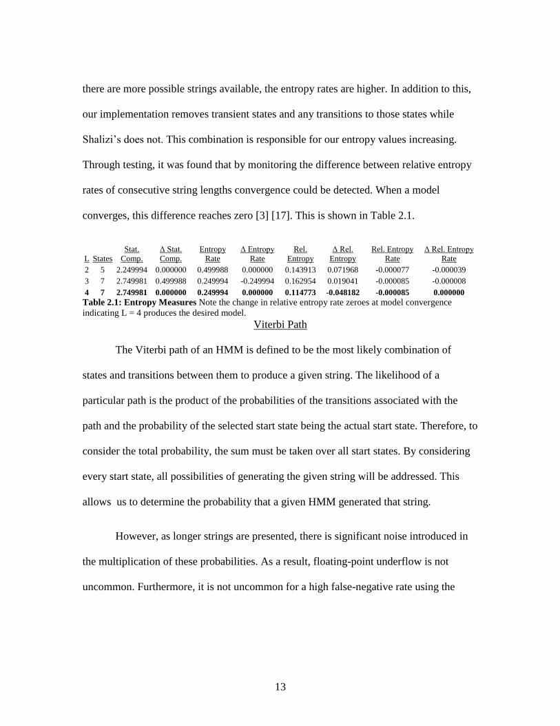
there are more possible strings available, the entropy rates are higher. In addition to this,
our implementation removes transient states and any transitions to those states while
Shalizi’s does not. This combination is responsible for our entropy values increasing.
Through testing, it was found that by monitoring the difference between relative entropy
rates of consecutive string lengths convergence could be detected. When a model
converges, this difference reaches zero [3] [17]. This is shown in Table 2.1.
L States
Stat.
Comp.
Δ Stat.
Comp.
Entropy
Rate
Δ Entropy
Rate
Rel.
Entropy
Δ Rel.
Entropy
Rel. Entropy
Rate
Δ Rel. Entropy
Rate
2 5 2.249994 0.000000 0.499988 0.000000 0.143913 0.071968 -0.000077 -0.000039
3 7 2.749981 0.499988 0.249994 -0.249994 0.162954 0.019041 -0.000085 -0.000008
4 7 2.749981 0.000000 0.249994 0.000000 0.114773 -0.048182 -0.000085 0.000000
Table 2.1: Entropy Measures Note the change in relative entropy rate zeroes at model convergence
indicating L = 4 produces the desired model.
Viterbi Path
The Viterbi path of an HMM is defined to be the most likely combination of
states and transitions between them to produce a given string. The likelihood of a
particular path is the product of the probabilities of the transitions associated with the
path and the probability of the selected start state being the actual start state. Therefore, to
consider the total probability, the sum must be taken over all start states. By considering
every start state, all possibilities of generating the given string will be addressed. This
allows us to determine the probability that a given HMM generated that string.
However, as longer strings are presented, there is significant noise introduced in
the multiplication of these probabilities. As a result, floating-point underflow is not
uncommon. Furthermore, it is not uncommon for a high false-negative rate using the
14
forward-backward procedure, which this is closely related to. To avoid both problems, a
confidence interval approach was adopted instead [4] [14].
Confidence Intervals
For a given Markov model, and the sequence of transitions (the delays), we
follow the transitions through the model to determine the probability that the model
generated that sequence. Every starting state is considered. Since the models generated by
CSSR are deterministic, if a symbol is encountered with no corresponding transition in
the model, the model is rejected as it could not have generated that sequence.
Every time there is a transition into or out of a state, counters for the state and
transition are incremented. By dividing the number of times a particular transition is
taken by the number of times the state is entered, an estimate of that transition probability
can be obtained. This allows us to define the confidence interval of this particular
transition as:
, /2 , , , /2 , ,(1 ) / , (1 ) /i j i j i j i i j i j i j ip Z p p c p Z p p c
Figure 2.6: Confidence Interval
Where pi,j is the transition probability from state i to state j, ci is the entry-counter for
state i, and Z /2 is from the standard Normal distribution. Since we possess these models,
the actual transition probabilities are known to us.
We can accept that our estimate for this transition is correct (sufficiently close to
the known transition probability) if it falls within this interval, with a false positive rate of
α. Note that if the frequency of transitions does not fall within this interval, the sequence
was not generated by this model, and the model is therefore rejected. These events,

15
detections and rejections, are also counted. If the rejection rate exceeds the threshold
calculated through use of receiver operating characteristic (ROC) curves, the model is
rejected. If the acceptance rate exceeds this threshold, the model is accepted [4].
We use an ROC curve to determine the threshold we use for detecting a behavior.
A ROC curve is the plot of the true positive rate against the false positive rate. An ideal
decision boundary would have an ROC curve which goes from the origin (0,0) to (1,0)
and then (1,1). The threshold chosen is the point on the curve closest to (1,0) [16].
Flipping a coin, in contrast, would have an ROC curve which goes from (0,0) to (1,1).
The closer the curve comes to (1,0), the better the decision boundary is.
In addition, we will compare the results from using the confidence intervals
against the results using a maximum-likelihood approach: the forward phase of the
forward-backward procedure. The forward-backward procedure has two phases. In the
first phase, the probability that a given HMM generated a string is determined by
multiplying the probabilities of all necessary transitions to the probability of starting in
the given state. The sum of these values is the probability that the model generated the
string. The second phase is retuning phase but is not used by us [1] [14]. It is important to
note that confidence interval analysis is a detection method, not a classification method.
That is, it will identify when a particular sequence exhibits the characteristics of a given
model, but it will not identify it as belonging to exclusively one model.

16
CHAPTER THREE
TEST ENVIRONMENT
Testing Procedure
To confirm the hypothesis that CSSR can be used to reconstruct the underlying
model of communication, which is tunneled through a SSH connection, simplistic client
and server applications were created. The server application requires a finite-state-model
(FSM) file, sequence length, and the port for which it should listen for
acknowledgements on. The client application requires the server IP and port, as well as a
port for it to accept the symbol sequence on. Both applications have an option for UDP,
in this case, the IP address of the other machine must also be specified, as UDP does not
create a channel to communicate over.
A simple two-state FSM, shown in Figure 3.1, was used for this purpose. Each
state has two possible transitions: either to the other state (90%), or to remain in the
current state (10%). Whenever a transition is made, the symbol associated with that
transition is transmitted from the server to the client application. Then the server waits for
a delay associated with the transmitted symbol before making the next transition. The
client is nothing more than a listener, leaving acknowledgements to the underlying
protocol (TCP). The delays used for the proof of concept were 100 ms for A and 900 ms
for B.
The test consists of 1000 symbols being transmitted from the server to the client.
Wireshark is run on the client to capture the network data which is then filtered for
symbol arrival events, and filtered again so only UNIX timestamps remain. A simple Perl

17
script is then used to compute changes between adjacent times. This file is presented to
CSSR with a mesh file. The mesh file is a comma-separated-file containing the expected
symbols and their ranges. These ranges were defined as 0 to 500 ms and 501 to 10000
ms, for A and B respectively. A ceiling of 10 seconds is used to account for unknown
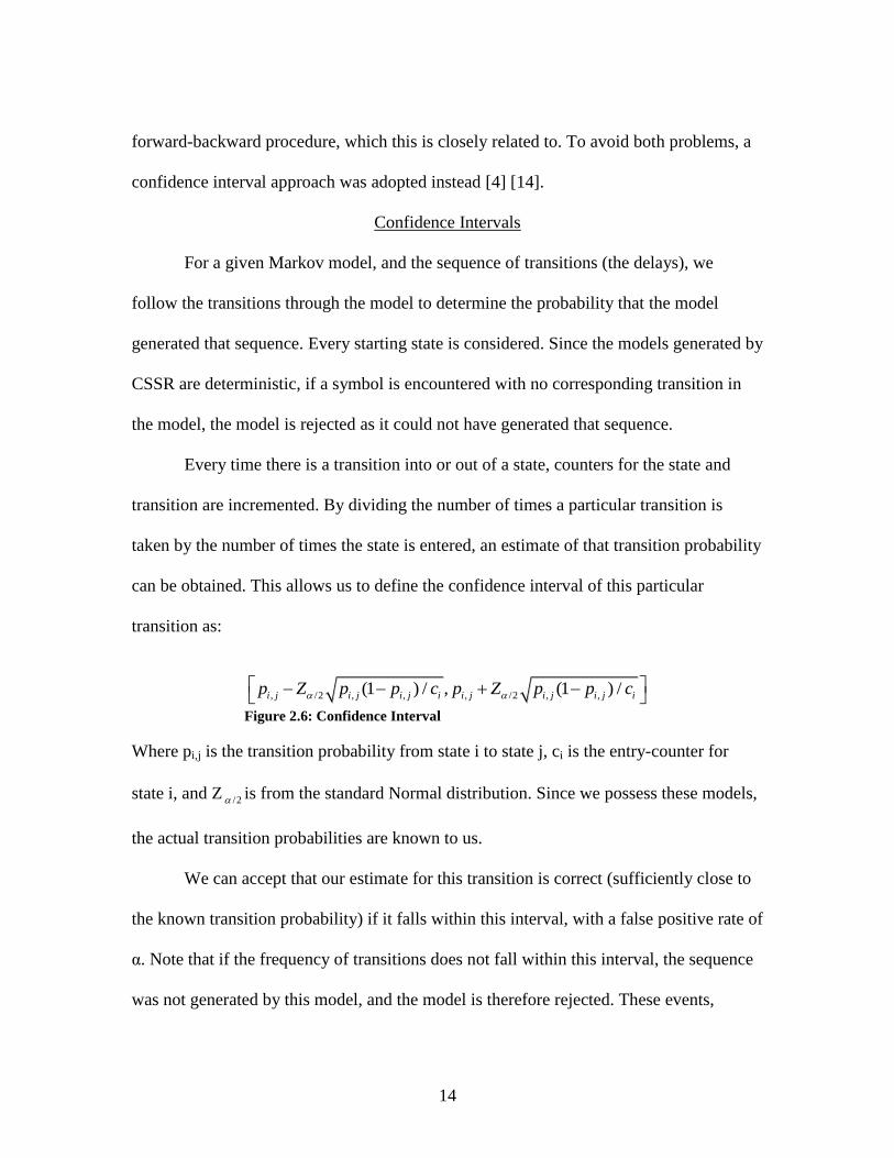
traffic. The computers were tested in two configurations, as shown in Figure 3.2 and 3.3.
In the first, they are directly connected, with only a switch in between, while in the
second there is an intermediary listener.
Figure 3.1: Two-State FSM
This test was repeated three times for each configuration, and the collected data
was processed by CSSR to create models. In all six cases, the original model was
successfully reconstructed. The reconstructed models are shown in Figure 3.4 and 3.5.
Furthermore, to determine the overhead introduced by the SSH tunnel, a spreadsheet was
used to keep track of the means and variances of unexpected delays for the trials. These
delays are the sum of clock skew, latency and SSH overhead as determined by a Matlab
script which compared the expected value to the observed. These means and variances

18
were then averaged among connection type, direct (plain-text) and SSH, and the
difference was taken. These results are in Table 3.1.
Figure 3.2: Direct Connection Configuration
19
Figure 3.3: Tunnel Configuration
Trial Plain SSH Tunnel
Mean (s) Variance (s2) A B Mean (s) Variance (s2) A B
1 9.05E-04 2.26E-08 0 0 8.88E-04 7.97E-08 0 0
2 9.29E-04 2.69E-07 0 0 9.11E-04 1.44E-06 0 0
3 9.40E-04 8.61E-07 0 0 0.0016 1.55E-04 82 81
Average for Plaintext Average for SSH Tunnel
Mean (s) Variance (s2) Mean (s) Variance (s2)
9.25E-04 3.84E-07 1.13E-03 5.21E-05
Overhead from SSH
Mean (s) Variance (s2)
2.08E-04 5.17E-05 Table 3.1: SSH Overhead
Model Reconstruction

20
The model below was reconstructed using CSSR with a string-length, L, of 3.
That is, only a history of two symbols are considered when conditional probabilities were
computed. The SSH differs from the expected model in the transition probabilities, but as
L increases it converges to the generating model. This occurs at L = 5.
Figure 3.4: Plain-Text Reconstruction
Figure 3.5: SSH Reconstruction
Findings
Though tunneling the transmission from the server introduces overhead – a
potential problem as it can lead to misclassification – reconstruction is possible with
sufficient data. The boundaries for the symbols can be determined by plotting a histogram

21
of the collected inter-packet delays. This will allow for clear identification of symbols. If
the range of collected data is too wide, as with the New Zealand keystroke statistics in
Chapter Four, a clustering application such as growing neural gas can be applied to
determine crucial centers of activity. Once these values are found, boundaries between
symbols can be defined as the midpoint between them.
An important factor to be kept in mind for reconstruction is the separation
between symbols as this defines the decision boundaries used. In these trials the
separation was 800 ms. For reconstruction to be successful, there must be enough space
between symbols so that there is as little overlap as possible. The reason for this is that a
maximum-likelihood separation is used to classify symbols when the midpoint between
delays is used as a decision boundary. The midpoint needs to be sufficiently far from the
lower boundary to account for latency, clock-skew, and overhead for the communication
channel. If these are not accounted for, misclassifications will occur, resulting in either
continuous state-space growth, as CSSR attempts to fit the model to the data, or complete
state-space collapse.
Having sufficient data is another concern with model reconstruction. If there is
not enough data, events which are statistically insignificant will become significant. As a
result, CSSR will continue to create states in an attempt to fit the model to the data
available to it.

22
CHAPTER FOUR
EXPERIMENTAL RESULTS
Patterns in Communications Channels
To determine if CSSR can properly reconstruct models for communication over a
secure channel, a single client-server application was created. The new application
contains two threads which run concurrently: a client thread, which listens for new
symbols, and the server thread which makes transitions and transmits the associated
symbol to the second application. For this configuration to more closely represent active
communication, the master and slave instances make the transition received from their
counterpart before generating their own. The two instances, however, do not need to use
the same FSM, provided the same alphabet is kept between the two machines.
The process, as shown in Figure 4.1, begins with the master application’s server
thread making a transition and sending the generated symbol to the slave application’s
client thread. The slave’s client thread, upon receiving the symbol, wakes its server
thread. This thread then makes the transition which was received followed by its
response, another transition. The server thread on the client then sends this symbol to the
master’s client thread.
While this communication is taking place, tshark is capturing the data that the
master application sends to the slave. However, as it is not capturing the returned data, a
hidden transition is present from its perspective.

23
Figure 4.1: Ping Pong Procedure

24
To determine the effect of this transition on the reconstruction process, the master
and slave applications were given the two-state FSM used for the proof of concept. The
delays associated with the symbols were changed for each of the three test cases, while
the transition probabilities were kept constant: the probability to change states was 90%
while the probability to remain was 10%. These delays are shown below in Table 4.1.
Trial Name Master Delay (ms) Slave Delay (ms)
A B A B
Overlap 1 300 360 10 40
Overlap 2 100 200 100 200
Separated 300 400 10 20 Table 4.1: Ping Pong Trial Delays
Since each FSM consists of two states, there are a total of four possible symbol
combinations which can be encountered: AA, AB, BA, and BB. To account for this, the
symbolization must use the midpoints of all four pairs. The exception for this is the case
“Overlap 2,” as AB and BA cause delays of identical lengths. Histograms were
constructed of the collected data to ensure that the ranges were being correctly assigned.
These histograms are shown in the following figures: Figure 4.2, 4.3 and 4.4.

25
Figure 4.2: Overlap 1 Delay Histogram
Figure 4.3: Overlap 2 Delay Histogram

26
Figure 4.4: Separated Delay Histogram
As expected, the midpoints between adjacent symbol-pairs allowed for
reconstruction. For the reconstruction process, 50000 symbols were generated for each
trial case. The delays were captured using a script which invoked tshark with a filter to
ignore any data not from the master to the slave. This was to prevent pollution of the data
from other network sources such as ARP, UPnP, and so on. Once the times were
collected, their deltas were computed and plotted to determine appropriate symbol
ranges. The deltas and symbol ranges were then provided to CSSR for analysis. Analysis
was started with the string length set to 3, and increased incrementally until a stable
machine was generated. That is, until the machine between consecutive iterations
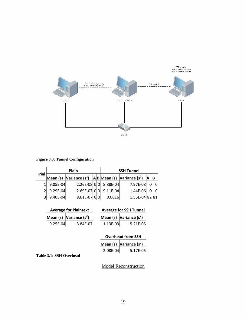
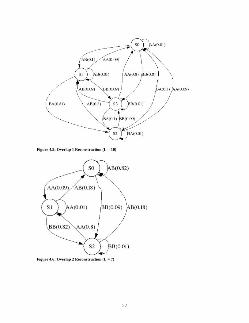
remained the same. The reconstructed FSM are shown below in Figure 4.5, 4.6 and 4.7.
27
Figure 4.5: Overlap 1 Reconstruction (L = 10)
Figure 4.6: Overlap 2 Reconstruction (L = 7)

28
Figure 4.7: Separated Reconstruction (L = 7)
Note that the final case, Separated – Figure 4.7, resulted in an identical FSM as
the first trial case, Overlap 1. This was expected as in both cases, there was sufficient
separation between individual symbol combinations to allow for proper distinction by
CSSR. However, the additional space between the masters’ symbols, coupled with the
fact that both symbols can be generated from either state, allows for the original two-state
FSM to be reconstructed as well as the joint machine. This joint machine is shown in
Figure 4.7
Both factors must be considered for this to be possible. If the original FSM does
not allow for transitions made by the client to be accounted for, then additional states will
be added to the state-space as the string length is increased. Furthermore, if the delays are
insufficiently separated, proper distinction between symbols will not be possible.

29
Clock-Skew Analysis
To test the hypothesis that devices in close physical proximity will maintain clock
synchronicity for longer periods of time between synchronizations than those far apart,
the original pair of applications used for the proof of concept were configured on three
machines. Two of these machines remained in the lab while the third was my desktop.
All three machines were configured to update their time periodically using NTP. The
machines in the lab were synchronized at varying rates while my desktop was kept
consistent at once every 4 hours.
Crontab was used to alter the rate at which the lab computers synchronized their
internal clocks, and after 24 hours of synchronizing at a particular rate, the client and
server applications were executed between the lab computers as well as between a lab
computer and my desktop. In all cases, the same 5000 symbol sequence was used, with a
15 ms difference between the delays associated for the symbols A and B. The reason for
this separation is 15 ms is the closest two symbols can be and still allow for proper
reconstruction when considering communication between my room and the lab.
As the rate at which the lab computers synchronize is reduced, more
misclassifications should take place between my desktop and the lab computers,
specifically for the symbol with the lower delay. Furthermore, the variance for extraneous
delays should increase for both communication channels as the clocks move further out
of synch.
The results of these trials are contained in the table below, Table 4.2. As expected,
the misclassifications increased as the computers were synchronized less frequently. This

30
trend is more apparent when considering the difference between lab computers over time.
The variance of the sum of latency and clock-skew, the unexpected delays monitored
here, increases consistently for intra-lab communications. Also, there is a significant
increase in this variance when moving from the lab environment to the campus intranet.
This is also expected as the data must pass through multiple copper/fiber relays between
the desktop in my apartment and the lab.
Location Synchronized Every 1 Hour Synchronized Every 2 Hours
[Latency + Clock Skew] Miss [Latency + Clock Skew] Miss
Mean (s) Variance (s2) A B Mean (s) Variance (s2) A B
Lab 9.06E-04 5.95E-09 0 0 9.06E-04 5.96E-09 0 0
Apartment 3.31E-04 2.72E-06 0 1 2.52E-04 2.31E-06 2 13
Synch/1 Hr to Synch/2 Hr
-4.00E-08 1.64E-11
-7.97E-05 -4.12E-07
Location Synchronized Every 3 Hours Synchronized Every 4 Hours
[Latency + Clock Skew] Miss [Latency + Clock Skew] Miss
Mean (s) Variance (s2) A B Mean (s) Variance (s2) A B
Lab 9.09E-04 1.36E-08 0 0 9.21E-04 2.03E-07 0 1
Apartment 3.00E-04 3.02E-06 5 10 2.65E-04 2.71E-06 2 5
Synch/2 Hr to Synch/3 Hr Synch/3 Hr to Synch/4 Hr
3.52E-06 7.62E-09 1.22E-05 1.90E-07
4.84E-05 7.07E-07 -3.54E-05 -3.05E-07
Synch/1 Hr to Synch/3 Hr Synch/2 Hr to Synch/4 Hr
3.48E-06 7.64E-09 1.57E-05 1.97E-07
-3.13E-05 2.95E-07 1.30E-05 4.02E-07
Synch/1 Hr to Synch/4 Hr
1.57E-05 1.97E-07
-6.67E-05 -1.00E-08 Table 4.2: Cron Clock Skew

31
Long-Range Analysis
In order to determine the closest separation acceptable for long-range LAN
communication to be symbolized, a computer was configured in my room to transmit a
known 5000 symbol sequence to the client in the lab. Symbols were initially separated at
12 ms. This starting value was chosen as it was marginally above the required separation
for within-lab communications. Upon constructing a histogram of the collected data,
Figure 4.8, the cause of failure with the symbolization was apparent. Attempting with a
15 ms separation, Figure 4.9, allowed for a successful separation between the symbols
and subsequent reconstruction.
Having determined that the closest separation between two symbols for successful
reconstruction within the lab is 10 ms, and that for intra-campus communication is 15 ms,
the next step was to find this value for internet communication. To accomplish this, my
colleague Ryan Craven set up his computer at his apartment to be the server, with the
client remaining within the lab. As with the clock-skew analysis, a known 5000 symbol
sequence defining the transitions taken by the server was used in conjunction with the
client-server applications from the proof of concept trials.
The separation began at 50 ms which was successful. A histogram of the collected
data, Figure 4.10, shows a distinct separation, though there is a noticeable amount of
overlap between the two symbols. Reducing to 40 ms, Figure 4.11, however, caused a
significant amount of overlap between the two symbols. As a result, proper symbolization
32
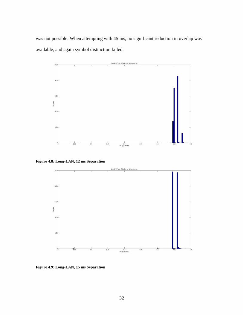
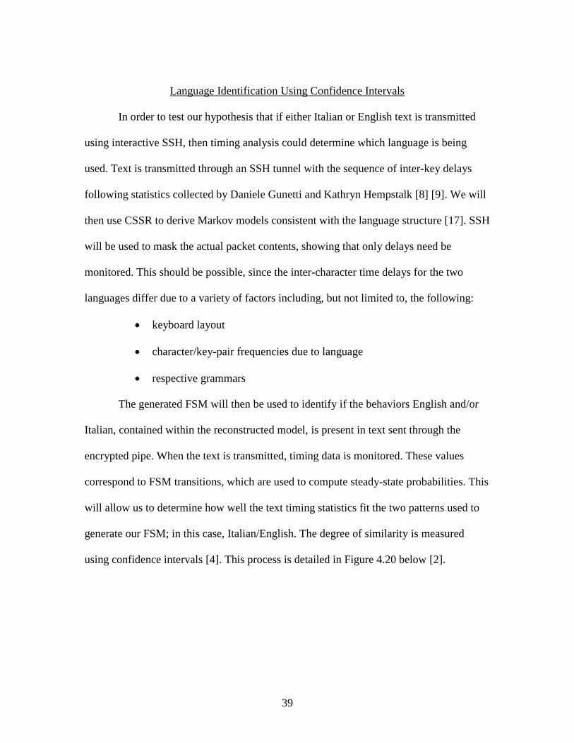
was not possible. When attempting with 45 ms, no significant reduction in overlap was
available, and again symbol distinction failed.
Figure 4.8: Long-LAN, 12 ms Separation
Figure 4.9: Long-LAN, 15 ms Separation

33
Figure 4.10: Off-Campus, 50 ms Separation
Figure 4.11: Off-Campus, 40 ms Separation
Furthermore, false-positive analysis was performed on all three locations. The
results of these tests are in Table 4.3. As expected, there is an increase in

34
misclassification as the distance between the computers increases. Similarly, there is a
noticeable increase in mean and variance of communication overhead.
[Latency + Skew] False Positives
Minimum Separation Mean (s) Variance (s2) A B Total
Short LAN 10 mSec 9.06E-04 5.95E-09 0 0 0
Long LAN 15 mSec 2.78E-04 2.77E-06 1 4 5
Internet 50 mSec 0.0102 1.67E-04 774 831 1605 Table 4.3: Long-Range False Positive Analysis
Identifying Methods of Communication with Definite State Structure
To simulate a more complex communication model, the ping-pong applications
were used with two sets of three-state FSM model pairs. That is, “model 4,” consists of a
three-state FSM running on the master node, ping, and a separate three-state FSM
running on the slave node, pong. Similarly, “model 5” consisted of different three-state
FSM being used for both ping and pong. These FSM are shown below in Figure 4.12
through Figure 4.15.
Figure 4.12: Model 4 – Ping

35
Figure 4.13: Model 4 – Pong
Figure 4.14: Model 5 – Ping

36
Figure 4.15: Model 5 - Pong
To ensure proper separation between symbols, the delays associated with pings’
symbols were 300, 360 and 420 ms, respectively for A, B and C. Pong’s symbol delays
were 10, 20 and 30 ms for A, B and C. A sequence of 50000 symbols were generated, to
ensure sufficient data was available for CSSR, and plotted in MatLab to ensure that
sufficient separation was present. The histograms below, Figures 4.16 and 4.17, show
that this constraint was met.
Upon finding that the two-state ping-pong system was able to regenerate the
model used by the master application, a similar test was presented to the data collected
here. By using the regions shown by the histograms to symbolize the data, the ping model
was successfully regenerated for both sets of models. The regenerated models are shown
in Figures 4.18 and 4.19, below.

37
Figure 4.16: Model 4 Histogram
Figure 4.17: Model 5 Histogram

38
Figure 4.18: Model 4 Ping Reconstruction
Figure 4.19: Model 5 Ping Reconstruction
39
Language Identification Using Confidence Intervals
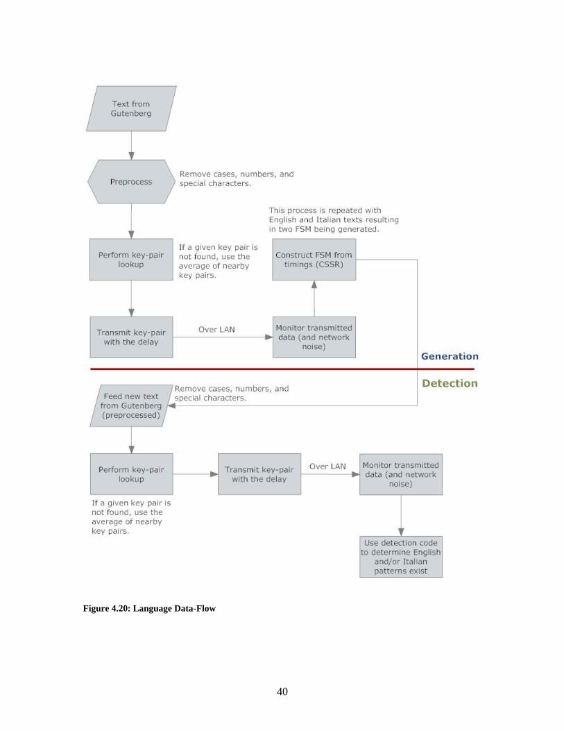
In order to test our hypothesis that if either Italian or English text is transmitted
using interactive SSH, then timing analysis could determine which language is being
used. Text is transmitted through an SSH tunnel with the sequence of inter-key delays
following statistics collected by Daniele Gunetti and Kathryn Hempstalk [8] [9]. We will
then use CSSR to derive Markov models consistent with the language structure [17]. SSH
will be used to mask the actual packet contents, showing that only delays need be
monitored. This should be possible, since the inter-character time delays for the two
languages differ due to a variety of factors including, but not limited to, the following:
keyboard layout
character/key-pair frequencies due to language
respective grammars
The generated FSM will then be used to identify if the behaviors English and/or
Italian, contained within the reconstructed model, is present in text sent through the
encrypted pipe. When the text is transmitted, timing data is monitored. These values
correspond to FSM transitions, which are used to compute steady-state probabilities. This
will allow us to determine how well the text timing statistics fit the two patterns used to
generate our FSM; in this case, Italian/English. The degree of similarity is measured
using confidence intervals [4]. This process is detailed in Figure 4.20 below [2].
40
Figure 4.20: Language Data-Flow

41
Using the data provided to us by Daniele Gunetti of Italy and Kathryn Hempstalk
of New Zealand, key-pair statistics were extracted for alphabets, numerals, enter, space,
and backspace, a total of 39 characters as case was ignored [8] [9]. These values were
used to populate a 39-by-39 delay matrix. By examining the keyboard layouts of the
Italian and New Zealand, English-International, keyboards, a39-by-4 matrix was
constructed of neighboring keys for those characters considered.
For any entry for which no value existed, the neighbor list for the destination key
was consulted. If sufficient data was present for similar key-pairs in which the destination
key belongs to the neighbor list, the missing value was updated with the average of the
neighbor key values. If insufficient data is present, however, the destination key is held
constant and the source key’s neighbor list is consulted. This process is repeated until the
matrix remains constant across two passes. These delays were then plotted in 3-D,
Figures 4.21 and 4.22, in an attempt to discern any obvious centers of activity. However,
given the range of delays encountered, this proved to be unhelpful.

42
Figure 4.21: Italian Interpolation
Figure 4.22: New Zealand Interpolation
43
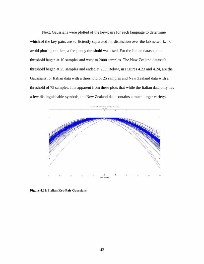
Next, Gaussians were plotted of the key-pairs for each language to determine
which of the key-pairs are sufficiently separated for distinction over the lab network. To
avoid plotting outliers, a frequency threshold was used. For the Italian dataset, this
threshold began at 10 samples and went to 2000 samples. The New Zealand dataset’s
threshold began at 25 samples and ended at 200. Below, in Figures 4.23 and 4.24, are the
Gaussians for Italian data with a threshold of 25 samples and New Zealand data with a
threshold of 75 samples. It is apparent from these plots that while the Italian data only has
a few distinguishable symbols, the New Zealand data contains a much larger variety.
Figure 4.23: Italian Key-Pair Gaussians

44
Figure 4.24: New Zealand Key-Pair Gaussians
This prompted me to process the data through an artificial neural network to
properly identify the means of the symbols. The results produced by growing neural gas,
Table 4.4, support the Gaussians as only two symbols were found within the Italian data.
Furthermore, a large number of means were identified within the New Zealand data
within the 220 ms range. Given the behavior of growing neural gas, creating more means
for areas that need to be better represented, this too follows from the plot of the Gaussian
data for New Zealand. However, given that symbols closer than 10 ms cannot be
successfully distinguished, they were replaced by one symbol whose mean is the average
of theirs, Table 4.5.

45
Italian New Zealand
Symbol Mean Symbol Mean
A 15.32 A 95.14
B 38.88 B 153.17
C 49.98 C 209.04
D 67.19 D 261.29
E 311.21
F 340.10
G 344.59
H 344.77
I 344.77
J 344.82
K 344.90
L 351.55
M 382.01
N 445.05
O 541.29
P 707.73 Table 4.4: Growing Neural Gas Means
Italian New Zealand
Symbol Mean Symbol Mean
A 15.32 A 95.14
B 38.88 B 153.17
C 49.98 C 209.04
D 67.19 D 261.29
E 311.21
F 345.07
G 382.01
H 445.05
I 541.29
J 707.73 Table 4.5: Final Symbolization
The training data for the FSM were selected from those available at
ProjectGutenberg that were published after 1900, or as close to it as possible, to keep the
language as current as possible. The texts used, and their release dates, are listed below in

46
Table 4.6. After stripping all non-alpha-numeric and non-whitespace characters from the
text, the values were converted to indices of the 39-by-39 delay matrix. Then, delays
were assigned to each pair of letters by using the previously constructed delay matrix as a
look-up table. Plotting histograms of these aggregates are shown below in Figures 4.24
and 4.25.
English Training Data (2165563 character pairs)
Agatha Christie - The Mysterious Affair at Styles (1916/20)
Sir Arthur Conan Doyle - Hound of the Baskervilles (1901)
Andre Norton - Plague Ship (1956)
Bram Stoker - Dracula (1897)
F. Anstey - The Brass Bottle (1900)
Italian Training Data (2285630 character pairs)
Luigi Barzini - L'Argentina Vista Come E (1902)
Enrico Annibale Butti - L'Immorale (1894)
Gabriele D'Annunzio - L'Innocente (1992)
Frederico De Roberto - Documenti Umani (1888)
Shakespeare/Diego Angeli (trans) - La Tempesta (1912)
Giuseppe Giacosa - Diritti Dell'Anima (1900)
Cletto Arrighi - Nana a Milano (1880)
Anton Guilio Barrili - Tra cielo e terra (2009) Table 4.6: Selected Texts – Gutenberg

47
Figure 4.25: Italian Gutenberg Data
Figure 4.26: New Zealand Gutenberg Data
Once each text was converted into sets of key-pairs and symbolized, they were
divided into a testing set and training set. The purpose of this was to ensure that the test
strings presented were from a source with similar patterns. This ensured that no
anomalies were presented in the test strings. The Italian training data consisted of

48
1,414,289 symbols, and the English training data contained 1,000,479 symbols. The
remaining symbols comprised the respective testing sets. The reconstructed models for
English and Italian are located in Appendix A, Figures A.9 and A.10, respectively.
Two strings of 100 symbols were taken from each testing set. These strings were
then used for a maximum-likelihood analysis using the forward-backward procedure.
Longer strings were not used due to the effect of multiplying large groups of numbers
less than 1. In addition, two strings were found online and presented to the machines. As
with the earlier strings, forward-backward analysis was performed. Confidence interval
analysis was then performed on all strings with respect to both reconstructed models, as
well as the training and testing sets with the same models. These results are shown in
Table 4.7. The strings taken from the testing data are identified as “str 1” and “str 2”
followed by the language whose testing set it belongs.
English (L = 1) Italian (L = 1) Italian (L = 2) Italian (L = 3)
Fwd/Bkwd Seqmatch Fwd/Bkwd Seqmatch Fwd/Bkwd Seqmatch Fwd/Bkwd Seqmatch
Str 1(Eng) 3.66E-81 100.00% 0.00E+00 0.00% 0.00E+00 0.00% 0.00E+00 0.00%
Str 2(Eng) 1.63E-86 95.00% 0.00E+00 0.00% 0.00E+00 0.00% 0.00E+00 0.00%
Str 3(Eng) 1.14E-167 94.00% 0.00E+00 0.00% 0.00E+00 0.00% 0.00E+00 0.00%
Str 4(Eng) 3.06E-255 95.00% 0.00E+00 0.00% 0.00E+00 0.00% 0.00E+00 0.00%
Train (Eng) 94.00% 0.00% 0.00% 0.00%
Test (Eng) 50.00% 0.00% 0.00% 0.00%
Str 1(Itl) 3.65E-111 90.00% 1.06E-50 0.00% 3.37E-50 0.00% 8.76E-50 99.21%
Str 2(Itl) 5.31E-125 86.00% 8.51E-51 100.00% 7.70E-51 100.00% 5.90E-51 98.81%
Str 3(Itl) 1.18E-273 83.00% 1.66E-111 100.00% 7.78E-109 98.44% 5.05E-107 99.60%
Str 4(Itl) 9.24E-271 83.00% 7.27E-109 100.00% 7.11E-107 100.00% 5.79E-103 98.81%
Train (Itl) 60.00% 100.00% 100.00% 100.00%
Test (Itl) 60.00% 12.50% 32.81% 50.59%
Table 4.7: Identification Results

49
In the above table, the columns marked “Seqmatch” correspond to the confidence
interval analysis for the given string-model pair with a 1% false positive rate. That is, the
likelihood that the given model generated the string with 99% confidence. The
“Fwd/Bkwd” columns contain the results of the maximum-likelihood analysis through
application of the forward-backwards procedure. As mentioned earlier, since it’s the
product of large quantities of probabilities, these values are expected to be extremely low.
The training and testing sets were not tested in this fashion for this reason, as there isn’t
enough accuracy available to get meaningful results.
Note that when English strings are presented to any of the Italian models, for
string lengths 1 through 3, it is rejected. But when Italian is presented to the English
model, it has a fairly high probability of being generated, as shown by the confidence
interval results. However, when the forward-backward analysis is examined, it is clear
that it is not a good fit. The difference between these values differ by several orders of
magnitude.
Using window size analysis developed by Jason Schwier [16], it was determined
that 77 symbols were required for maximum-likelihood classification using confidence
intervals. That is, with at least 77 symbols presented to the English and Italian
reconstructions, a majority of the time it would be correct. By dividing the testing set into
samples of 77 strings, a series of detection percentages were calculated through
confidence interval analysis.
Plotting the true positives and false positives together against the acceptance
threshold, while varying the threshold, generated the receiver operating characteristic

50
curves (ROC curves) shown below. This allows us to determine the ideal acceptance
threshold for separation for presented strings between the two models.
Figure 4.27: English ROC – 95% CI
Figure 4.28: Italian ROC – 95% CI

51
Thresh. True Pos False Pos True Neg False Neg Distance
0.00 401 401 0 0 1.000
[Repeated 79 times]
0.80 401 401 0 0 1.000
0.81 401 392 9 0 0.978
0.82 401 371 30 0 0.925
0.83 401 294 107 0 0.733
0.84 401 201 200 0 0.501
0.85 401 103 298 0 0.257
0.86 401 40 361 0 0.100
0.87 401 9 392 0 0.022
0.88 399 3 398 2 0.009
0.89 399 0 401 2 0.005
0.90 397 0 401 4 0.010
0.91 390 0 401 11 0.027
0.92 367 0 401 34 0.085
0.93 367 0 401 34 0.085
0.94 264 0 401 137 0.342
0.95 188 0 401 213 0.531
0.96 113 0 401 288 0.718
0.97 41 0 401 360 0.898
0.98 14 0 401 387 0.965
0.99 1 0 401 400 0.998
1.00 0 0 401 401 1.000
Table 4.8: English ROC – 95% CI – Statistics
Thresh. True Pos False Pos True Neg False Neg Distance
0.00 397 0 401 4 0.009975
[Repeated 93 times]
0.94 397 0 401 4 0.009975
0.95 381 0 401 20 0.049875
0.96 354 0 401 47 0.117207
0.97 245 0 401 156 0.389027
0.98 117 0 401 284 0.708229
0.99 14 0 401 387 0.965087
1.00 0 0 401 401 1
Table 4.9: Italian ROC – 95% CI – Statistics

52
From Figures 4.27 and 4.28, it is apparent that the 95% CI used to determine the
presence of English and/or Italian characteristics in the strings is sufficient. Upon
examination of the statistics used to produce the ROC curves, Table 4.8 and 4.9, it was
discovered that an 89% threshold would be sufficient. That is, with a 95% CI, a decision
boundary at 89% would have the best classification rate for both languages. To compare
the confidence interval analysis to the standard maximum-likelihood classifier, the
forward-backward procedure was used. The ROC curves in Figures 4.29 and 4.30 show
these results. This shows that while there are slightly more false positives when using
confidence intervals, it is more forgiving as the string length increases. Also, there are
fewer false negatives with CI than with a maximum-likelihood classifier.
Figure 4.29: English ROC -- ML (Forward-Backward)
53
Figure 4.30: Italian ROC -- ML (Forward-Backward)

54
CHAPTER FIVE
CONCLUSIONS
Through timing analysis and the application of Hidden Markov Models, we have
shown that it is possible to identify the communication behavior in use, even over a
secure communication channel. This behavior may even be the language that the user is
typing in [2]. For proper reconstruction to be possible, two requirements must be met:
there must be sufficient data to model the communication observed, and there must be
sufficient delays between symbols.
When there is insufficient data there are two possible outcomes: the state-space
will grow resulting in a state-explosion, or the proper model will be reconstructed with
incorrect transition probabilities. The reason for the first case is that because there was
not enough data, aberrations were given statistical significance. Since CSSR attempts to
minimize entropy, it continues to add states to better fit the data given it. In the second
case, there is sufficient data for the model to be reconstructed, but not enough to properly
determine the transition probabilities, and consequently the steady state probabilities.
It was also shown that when a hidden transition was present in the communication
channel, as in the case of ping-pong with one observer, it is possible to reconstruct the
joint state model as well as the dominating model. Again, this is only possible when there
is sufficient separation between the symbols. As this separation is decreased, instead of
reconstructing the dominating model, the model used by the observer is reconstructed [3].

55
CHAPTER SIX
FUTURE WORK
There are many possibilities for the application of Hidden Markov Models.
Presently, they are used largely for speech-to-text conversion and biometric analysis. By
incorporating confidence intervals, however, the speech-to-text conversion should
become more accurate. This is because though there is a higher false positive rate
associated with confidence intervals, there is a larger true positive rate as well.
Furthermore, as strings become longer, maximum likelihood suffers from degradation
due to large sets of numbers between 0 and 1 being multiplied together. This is not a
problem for confidence intervals. It could be argued that the false positive rate, even
though it is marginal, is undesirable for security applications given the risk involved.
Additionally, given the nature of Causal State Splitting Reconstruction, it should
be possible to construct a HMM that is “trained” on the works of a specific author. This
HMM, in conjunction with confidence interval analysis, can then be used to assist in
identification of previously unidentified works. Since each author has a unique style,
CSSR should be able to identify this pattern and the state history present in the HMM
will reflect it. There will need to be a substantial training set, however, as the string
length required to discern these patterns may be well above 10, and a sufficiently large
data set will be required to ensure that events are not improperly given statistical
significance.
With more data available, the interpolation phase performed to fill in gaps present
in the delay matrix would not be required. This would allow for a more accurate

56
symbolization which in turn leads to better detection. A larger amount of data would also
allow for a better symbolization to be found outright, as there should be a larger spread of
delays. This would, again, lead to a better detection. Ideally the data used to extract the
key-pair statistics would contain special characters, different case, and so on. As ours
lacked these, we had to preprocess the text from ProjectGutenberg to fit the data
available. By having case-sensitivity, special characters, etc, new patterns can be detected
in the training/testing data allowing for a more complete representation in the HMM.

57
APPENDICES

58
Appendix A
Ancillary Information
Keyboard Layout Comparison
A major factor contributing to inter-keystroke delay is the layout of the keyboard.
Therefore, the keyboards used by Italians and New Zealanders needed to be compared to
determine if keys possessed different neighbors and positions. The reason for this is two-
fold: to determine if keyboard layout played a part in the delays used in our language
detection experiment, and to determine the neighboring keys to interpolate delays for
missing keystroke pairs.
To compare the Italian and New Zealand keyboard layouts, Wapedia1 was
consulted. In comparing the two layouts, it was discovered that for the characters
monitored for this experiment were in identical locations. The left Shift key and Enter
keys were of different sizes and shapes, however, for the Italian keyboard. Both keyboard
layouts are shown below in Figures A.1 and A.2. They are reproduced under the Creative
Commons Attribution/Share-Alike License2 and GNU Free Documentation License
3.
Figure A.1: Italian Keyboard Layout (http://wapedia.mobi/en/File:KB_Italian.svg)
1 http://wapedia.mobi/en/Keyboard_layout
2 http://creativecommons.org/licenses/by-sa/3.0/
3 http://wapedia.mobi/en/Wikipedia:Text_of_the_GNU_Free_Documentation_License

59
Figure 4: New Zealand/US Keyboard Layout (http://wapedia.mobi/en/File:KB_United_States-
NoAltGr.svg)
Delay Matrix Reordering
The 39-by-39 delay matrix used is ordered as follows: A, B… Z, 0, 1 … 9, enter,
backspace, and space. Other orderings were considered based on keyboard cross-sections,
however. Both horizontal and vertical cross-sections were considered to see if one
provided a “smoother” plot than the original. These graphs are shown below.
Figure A.3: Italian - Original Ordering

60
Figure A.4: Italian - Horizontal Reordering
Figure A.5: Italian - Vertical reordering

61
Figure A.6: New Zealand - Original Ordering
Figure A.7: New Zealand - Horizontal Reordering

62
Figure A.8: New Zealand - Vertical Reordering
Comparing Figures A.8 to A.6 and Figures A.5 to A.3, it is apparent that a vertical
reordering offers smoother transitions between keystroke-pairs within the delay matrix.
This is more visible within the New Zealand data. This relationship is not unsurprising as
given home-row typing practices; the same finger is used for keys vertically adjacent to
one another, so more similar delays for those keys is reasonable.

63
Language Models
The models reconstructed from the texts sampled from ProjectGutenberg are
shown below. For each value of L considered, a statistical test was performed to ensure
that with the given alphabet and model, sufficient samples were available to ensure that
the model remained statistically significant. Only enough data was available for a string
length of 1 for English, and 3 for Italian.
During low-symbol-separation analysis it was found that if insufficient data or
separation was available, there was a threshold that allowed the model to be reconstructed
with incorrect transition probabilities between the states. This was attributed to statistical
significance being given to noise which would be discarded were there more samples.
Furthermore, it was estimated that at least 50 times more data, for each language, would
be required to consider larger string lengths.
To display the models as large as possible, only one is present on each page.

64
Figure A.9: English HMM, L = 1, 10 states, 100 transitions

65
Figure A.10: Italian HMM, L = 3, 64 states, 253 transitions
66
Old English and Latin
In an effort to determine the ability of the reconstructed HMMs for English and
Italian to detect the presence of similar languages being typed, ProjectGutenberg was
once again consulted. The texts selected were “Beowulf” and “Inferno,” for Old English
and Latin, respectively. Both texts were stripped of case and special characters, as with
the earlier texts. They were then symbolized with the delays used by their modern
counterparts: “Beowulf” with the New Zealand key-pair statistics, and “Inferno” with the
Italian. Next, 400 strings of 77 symbols were extracted from various locations from
within the two texts. These strings were presented to both reconstructed models for
confidence interval analysis and maximum-likelihood classification. These results are
presented in the ROC curves below in Figures A.11 through A.14.
Figure A.11: ROC Curve -- "Beowulf," 95% CI

67
Figure A.12: ROC Curve -- "Beowulf," ML
Figure A.13: ROC Curve -- "Inferno," 95% CI
68
Figure A.14: ROC Curve -- "Inferno," ML
It is evident from the ROC curves above that there is either sufficient similarity
between either the two pairs of languages or between the resulting symbolization. To
determine which of these was the case, two experiments were performed. In the first
experiment, English text was symbolized using the Italian delay statistics and symbol
alphabet, and Italian was symbolized with the English values. These cross-symbolizations
were then presented to the English and Italian HMMs for detection and classification.
Note that in the following ROC curves, Figures A.15 through A.18, the curves take a
fairly high threshold to allow any true positive classifications. This implies that the
models are recognizing the symbolization over the patterns in the language themselves.

69
Figure A.15: ROC Curve -- English with Italian Symbolization, 95% CI
Figure A.16: ROC Curve -- English with Italian Symbolization, ML

70
Figure A.17: ROC Curve -- Italian with English Symbolization, 95% CI
Figure A.18: ROC Curve -- Italian with English Symbolization, ML
The second experiment takes was performed to verify the hypothesis that the
models were, in fact, detecting the symbolization and not the patterns inherent to the

71
languages. This was accomplished by taking texts in languages with no Sanskrit roots,
but still represented through the use of Latin characters, and symbolizing with both the
English and Italian statistics. The purpose of this was to sufficiently separate the language
from English and Latin so that there would be no doubt in what was being detected.
72
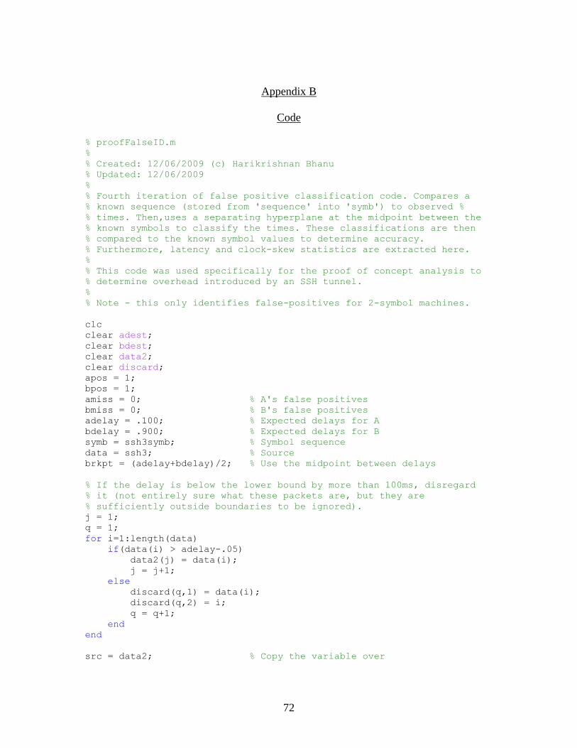
Appendix B
Code
% proofFalseID.m
%
% Created: 12/06/2009 (c) Harikrishnan Bhanu
% Updated: 12/06/2009
%
% Fourth iteration of false positive classification code. Compares a
% known sequence (stored from 'sequence' into 'symb') to observed %
% times. Then,uses a separating hyperplane at the midpoint between the
% known symbols to classify the times. These classifications are then
% compared to the known symbol values to determine accuracy.
% Furthermore, latency and clock-skew statistics are extracted here.
%
% This code was used specifically for the proof of concept analysis to
% determine overhead introduced by an SSH tunnel.
%
% Note - this only identifies false-positives for 2-symbol machines.
clc
clear adest;
clear bdest;
clear data2;
clear discard;
apos = 1;
bpos = 1;
amiss = 0; % A's false positives
bmiss = 0; % B's false positives
adelay = .100; % Expected delays for A
bdelay = .900; % Expected delays for B
symb = ssh3symb; % Symbol sequence
data = ssh3; % Source
brkpt = (adelay+bdelay)/2; % Use the midpoint between delays
% If the delay is below the lower bound by more than 100ms, disregard
% it (not entirely sure what these packets are, but they are
% sufficiently outside boundaries to be ignored).
j = 1;
q = 1;
for i=1:length(data)
if(data(i) > adelay-.05)
data2(j) = data(i);
j = j+1;
else
discard(q,1) = data(i);
discard(q,2) = i;
q = q+1;
end
end
src = data2; % Copy the variable over

73
for i=1:min(length(symb),length(data2));
% If it's greater than the threshold, it's a B, else, it's an A
if(src(i) >= brkpt)
% Determine the latency
bdest(bpos) = abs(src(i) - bdelay);
bpos = bpos + 1;
% Was it properly classified?
if(strcmp(symb(i),'B')~=1)
bmiss = bmiss + 1;
end
else
% Determine the latency
adest(apos) = abs(src(i) - adelay);
apos = apos + 1;
% Was it properly classified?
if(strcmp(symb(i),'A')~=1)
amiss = amiss + 1;
end
end
end
amiss
amean = mean(adest)
avar = var(adest)
bmiss
bmean = mean(bdest)
bvar = var(bdest)
tmean = mean([adest bdest])
tvar = var([adest bdest])

74
% histBound.m
%
% Created: 12/02/09 (c) Harikrishnan Bhanu
% Updated: 12/03/09
%
% Plots a histogram over a specified range, with a specified number of
% bins, from a given data-set. The segment of the dataset which is
% plotted is returned to the user.
function [ set ] = histBound( data, low, high, bins )
% Begin by sorting the data-set and searching for the lower and
% upper bounds
S = sort(data);
% Ensure that the low and high variables are entered in the proper
% order
low1 = min(low,high);
high1 = max(low,high);
low = low1;
high = high1;
% Force plot to search over the more constrictive restraints: those
% presented by the user, or the contents of the data-set.
if(low < S(1))
low = S(1);
end
if(high > S(length(S)))
high = S(length(S));
end
% Ensure the low and high bounds are valid for the given data-set
if(low > S(length(S)) || high < S(1))
fprintf('Invalid boundaries for the data-set.\n');
set = [];
else
% Search for the segment to plot
% Find the lower boundary in the data-set
for lowPos = 1:length(S)
if( S(lowPos) <= low && S(lowPos+1) >= low)
break;
end
end
% Find the higher boundary in the data-set. Don't bother
% searching below where the lower boundary was found, since the
% higher boundary can't be there.
for highPos = lowPos:length(S)
if( S(highPos) <= high && S(highPos+1) >= high)
break;
end
end
75
% Plot the portion of the data-set that we're interested in
hist(S(lowPos:highPos),bins);
set = S(lowPos:highPos);
end
end

76
% falsePositive3.m % % Created: 10/20/2009 (c) Harikrishnan Bhanu % Updated: 12/03/2009 % % Third iteration of false positive classification code. Compares a
% known sequence (stored from 'sequence' into 'symb') to observed
% times. Then, uses a separating hyperplane at the midpoint between the
% known symbols to classify the times. These classifications are then
% compared to the known symbol values to determine accuracy.
% Furthermore, latency and clock-skew statistics are extracted here. % % Note - this only identifies false-positives for 2-symbol machines.
clc clear adest; clear bdest; clear data2; clear discard; apos = 1; bpos = 1; amiss = 0; % A's false positives bmiss = 0; % B's false positives adelay = .345; % Expected delays for A bdelay = .360; % Expected delays for B symb = sequence; % Symbol sequence data = skew1dorm; % Source brkpt = (adelay+bdelay)/2; % Use the midpoint between delays to
differentiate
% If the delay is below the lower delay by more than 100ms, disregard
it % (not entirely sure what these packets are, but they are sufficiently % outside boundaries to be ignored). j = 1; q = 1; for i=1:length(data) if(data(i) > adelay-.1) data2(j) = data(i); j = j+1; else discard(q,1) = data(i); discard(q,2) = i; q = q+1; end end
src = data2; % Copy the variable over
for i=1:min(length(symb),length(data2)); % If it's greater than the threshold, it's a B, else, it's an A if(src(i) >= brkpt) % Determine the latency

77
bdest(bpos) = abs(src(i) - bdelay); bpos = bpos + 1;
% Was it properly classified? if(strcmp(symb(i),'B')~=1) bmiss = bmiss + 1; end
else % Determine the latency adest(apos) = abs(src(i) - adelay); apos = apos + 1;
% Was it properly classified? if(strcmp(symb(i),'A')~=1) amiss = amiss + 1; end end end
amiss amean = mean(adest) avar = var(adest) bmiss bmean = mean(bdest) bvar = var(bdest) tmean = mean([adest bdest]) tvar = var([adest bdest])

78
% parser2IT.m % % Created: 11/19/2009 (c) Harikrishnan Bhanu % Updated: 12/13/2009 % % Loads text sample files for parsing and outputs the delays for
% individual keypairs into separate files.File names have the format
% [key1]_[key2].txt and contain nothing but delays. % % Files are NOT generated for any symbol which is not alphanumeric,
% enter, space, or backspace. Furthermore, case is ignored: a -> Z will
% be treated as A -> Z. % % These files are then opened and statistics are extracted and the
% results are saved in statistics.txt % % Statistics.txt's contents follow the format: % [key1] [key2] [mean] [variance] [count] % without brackets.
% Flush variables to prevent pollution clear;clc;
% Get information of all files in the directory files = dir('./ItalianSrc/*'); q = 1;
% Loop through the files for i=3:length(files)
% Make sure there's no cross-session pollution clear temp; temp = load(sprintf('./ItalianSrc/%s',files(i).name));
% Extract all the pairs in the data for this sample for j=2:(length(temp)-2) source(q) = temp(j); delay(q) = temp(j+1); dest(q) = temp(j+2); q = q + 1; j = j + 1; end end
% Write these values out to files for i=1:length(source) last = source(i); next = dest(i); time = delay(i);
% Ensure only ASCII values are written if(last >= 0 && last <= 127 && next >= 0 && next <= 127)

79
% Force capitalization, and ensure only desired characters % are written if(last > 96 || last < 123) last = last - 22; end
if(next > 96 || next < 123) next = next - 22; end
% Ensure the last keystroke is from a valid key if ((last > 47 && last < 58) || (last == 32) || (last == 8) ||
(last == 13 || last == 10) || (last > 64 && last < 90))
% Repeat the check for the destination key if ((next > 47 && next < 58) || (next == 32) || (next == 8)
|| (next == 13 || next == 10) || (next > 64 && next < 90))
if(floor(last)==last && floor(next)==next) destfname = sprintf('%d_%d.txt',last,next); fout = fopen(destfname, 'a+'); fprintf(fout,'%f\n',time); fclose(fout); end
end
end end end
% Flush variables and screen clear;clc;
% Load the text files that were just generated clear files; textfiles = dir('*.txt'); meanVal = zeros(length(textfiles),1); varVal = zeros(length(textfiles),1); sampleSize = zeros(length(textfiles),1); outliers = zeros(length(textfiles),1);
for i=1:length(textfiles) temp = load(textfiles(i).name);
% Remove any negative values (artifacts of capture) temp(temp < 0) = [];
% Determine mean and variance for this keystroke pair sampleSize(i) = length(temp);

80
meanVal(i) = mean(temp); varVal(i) = var(temp); end
% Write this data to a textfile outFile = fopen('statisticsIT.txt','w+'); for i=1:length(textfiles)
% Extract the characters used from the file name
lastst1 = textfiles(i).name(1:strfind(textfiles(i).name,'_')-1); nextst1 =
textfiles(i).name(strfind(textfiles(i).name,'_')+1:strfind(textfiles(i)
.name,'.')-1);
% Convert from strings to numbers last = str2num(lastst1); next = str2num(nextst1);
% Replace the ASCII values with the corresponding indices for the
% 39x39 matrix if (last > 64 && last < 90) last = last - 64; elseif (last > 47 && last < 58) last = last - 47 + 26; elseif (last == 8) last = 37; elseif (last == 32) last = 38; elseif (last == 13) last = 39; end
if (next > 64 && next < 90) next = next - 64; elseif (next > 47 && next < 58) next = next - 47 + 26; elseif (next == 8) next = 37; elseif (next == 32) next = 38; elseif (next == 13) next = 39; end
fprintf(outFile,'%d %d %.3f %.3f
%d\n',last,next,meanVal(i),varVal(i),sampleSize(i)); end
fclose(outFile);

81
% parser2NZ.m % % Created: 11/19/2009 (c) Harikrishnan Bhanu % Updated: 12/13/2009 % % Loads text sample files for parsing and outputs the delays for
% individual keypairs into separate files.File names have the format
% [key1]_[key2].txt and contain nothing but delays. % % Files are NOT generated for any symbol which is not alphanumeric,
% enter, space, or backspace. Furthermore, case is ignored: a -> Z will
% be treated as A -> Z. % % These files are then opened and statistics are extracted and the
% results are saved in statistics.txt % % Statistics.txt's contents follow the format: % [key1] [key2] [mean] [variance] [count] % without brackets.
% Flush variables to prevent pollution clear;clc;
% Load sm-150 data load('./NZSrc/sm-150.mat');
for q1 = 1:10 for q2 = 1:15
% Define source vector, clear destination from possible
% previous runs clear dest; % Look at each sample independently src = evalin('base',char(sprintf('u%ds%d',q1,q2))); dpos = 1; last = 0;
% Prase the data from the .mat file for i=1:length(src) if mod(i,4) == 1 dest(dpos) = src(i)/2; dpos = dpos+1; elseif mod(i,4) == 0 dest(dpos) = src(i); dpos = dpos+1; end end
% Save the separated values into i = 1; last = dest(i); time = dest(i+1);

82
next = dest(i+2); while i<(length(dest)-2) % Ensure only ASCII values are written if(last >= 0 && last <= 127 && next >= 0 && next <= 127)
% Force capitalization, and ensure only desired
% characters are written if(last > 96 || last < 123) last = last - 22; end
if(next > 96 || next < 123) next = next - 22; end
% Equate enter and newline if(last == 10) last = 13; end
if(next == 10) next = 13; end
% Ensure the last keystroke is from a valid key if ((last > 47 && last < 58) || (last == 32) || (last
== 8) || (last == 13) || (last > 64 && last < 90))
% Repeat the check for the destination key if ((next > 47 && next < 58) || (next == 32) ||
(next == 8) || (next == 13) || (next > 64 && next < 90))
if(floor(last)==last && floor(next)==next) destfname = sprintf('%d_%d.txt',last,next); fout = fopen(destfname, 'a+'); fprintf(fout,'%f\n',time); fclose(fout); end
end
end end
% Move to the next character pair i = i + 2; last = dest(i); time = dest(i+1); next = dest(i+2);

83
end end end
% Clear variables clear;clc;
% Load the text files that were just generated files = dir('*.txt'); meanVal = zeros(length(files),1); varVal = zeros(length(files),1); sampleSize = zeros(length(files),1); outliers = zeros(length(files),1);
for i=1:length(files) temp = load(files(i).name);
% Convert from milliseconds to seconds % temp = temp./1000;
% Remove any negative values (artifacts of capture) temp(temp < 0) = [];
% Determine mean and variance for this keystroke pair sampleSize(i) = length(temp); meanVal(i) = mean(temp); varVal(i) = var(temp); end
% Write this data to a textfile outFile = fopen('statisticsNZ.txt','w+'); for i=1:length(files)
% Extract the characters used from the filename lastst1 = files(i).name(1:strfind(files(i).name,'_')-1); nextst1 =
files(i).name(strfind(files(i).name,'_')+1:strfind(files(i).name,'.')-
1);
% Convert from strings to numbers last = str2num(lastst1); next = str2num(nextst1);
% Replace the ASCII values with the corresponding indices for the
% 39x39 matrix if (last > 64 && last < 90) last = last - 64; elseif (last > 47 && last < 58) last = last - 47 + 26; elseif (last == 8) last = 37; elseif (last == 32)
84
last = 38; elseif (last == 13) last = 39; end
if (next > 64 && next < 90) next = next - 64; elseif (next > 47 && next < 58) next = next - 47 + 26; elseif (next == 8) next = 37; elseif (next == 32) next = 38; elseif (next == 13) next = 39; end
fprintf(outFile,'%d %d %.3f %.3f
%d\n',last,next,meanVal(i),varVal(i),sampleSize(i)); end
fclose(outFile);

85
% parser3.m % % Created: 11/10/2009 (c) Harikrishnan Bhanu % Updated: 12/13/2009 % % Loads text sample files for parsing and outputs the delays for
% individual keypairs into separate files.File names have the format
% [key1]_[key2].txt and contain nothing but delays. % % These files are then opened and statistics are extracted and the
% results are saved in statistics.txt
% % Statistics.txt's contents follow the format:
% {key1} --> {key2} , mean: [mean] , variance: [variance] , samples:
% [count] % Without brackets, but with braces.
clear;clc; load('sm-150.mat');
for q1 = 1:10 for q2 = 1:15
% Define source vector, clear destination from possible
previous % runs clear dest; % Look at each sample independently src = evalin('base',char(sprintf('u%ds%d',q1,q2))); dpos = 1; last = 0;
% Prase the data from the .mat file for i=1:length(src) if mod(i,4) == 1 dest(dpos) = src(i)/2; dpos = dpos+1; elseif mod(i,4) == 0 dest(dpos) = src(i); dpos = dpos+1; end end
% Save the separated values into i = 1; last = dest(i); time = dest(i+1); next = dest(i+2); while i<(length(dest)-2) % Ensure only ASCII values are written if(last >= 0 && last <= 127 && next >= 0 && next <= 127) if(floor(last)==last && floor(next)==next) destfname = sprintf('%d_%d.txt',last,next);
86
fout = fopen(destfname, 'a+'); fprintf(fout,'%f\n',time); fclose(fout); end end
% Move to the next character pair i = i + 2; last = dest(i); time = dest(i+1); next = dest(i+2); end end end
% Clear variables clear;clc;
% Load the text files that were just generated files = dir('*.txt'); meanVal = zeros(length(files),1); varVal = zeros(length(files),1); sampleSize = zeros(length(files),1); outliers = zeros(length(files),1);
for i=1:length(files) temp = load(files(i).name);
% Convert from milliseconds to seconds temp = temp./1000;
% Remove any negative values (artifacts of capture) temp(temp < 0) = [];
% Determine mean and variance for this keystroke pair sampleSize(i) = length(temp); meanVal(i) = mean(temp); varVal(i) = var(temp); end
% Write this data to a textfile outFile = fopen('statistics.txt','w+'); for i=1:length(files)
% Extract the characters used from the filename lastst1 = files(i).name(1:strfind(files(i).name,'_')-1); nextst1 =
files(i).name(strfind(files(i).name,'_')+1:strfind(files(i).name,'.')-
1);
% Convert from strings to numbers last = str2num(lastst1);

87
next = str2num(nextst1);
% If the values are between 34 and 126, convert it to the displayed
% char. Otherwise, replace it with something easy to determine. If
% the value is greater than 127, it's not an ASCII value, so
% disregard it. if (last < 33) switch last case 0 laststr = '{null}'; case 1 case 2 case 3 case 4 case 5 case 6 case 7 laststr = '{bell}'; case 8 laststr = '{backspace}'; case 9 laststr = '{tab}'; case 10 laststr = '{new line}'; case 11 laststr = '{vtab}'; case 12 laststr = '{new page}'; case 13 laststr = '{enter}'; case 14 laststr = '{shiftout}'; case 15 laststr = '{shiftin}'; case 27 laststr = '{esc}'; case 32 laststr = '{space}'; otherwise laststr = ['{' num2str(last) '}']; end else if(last < 127) laststr = char(last); elseif(last==127) laststr = '{del}'; else laststr = sprintf('%d',last); end end
if (next < 33) switch next

88
case 0 nextstr = '{null}'; case 1 case 2 case 3 case 4 case 5 case 6 case 7 nextstr = '{bell}'; case 8 nextstr = '{backspace}'; case 9 nextstr = '{tab}'; case 10 nextstr = '{new line}'; case 11 nextstr = '{vtab}'; case 12 nextstr = '{new page}'; case 13 nextstr = '{enter}'; case 14 nextstr = '{shiftout}'; case 15 nextstr = '{shiftin}'; case 27 nextstr = '{esc}'; case 32 nextstr = '{space}'; otherwise nextstr = ['{' num2str(next) '}']; end else if(next < 127) nextstr = char(next); elseif(last==127) nextstr = '{del}'; else nextstr = sprintf('%d',next); end end
% Only save information when at least 5 samples were collected if(sampleSize(i) > 5) fprintf(outFile,'%s --> %s mean: %.3f , variance: %.3f ,
samples: %d\n',laststr,nextstr,meanVal(i),varVal(i),sampleSize(i)); end
end
fclose(outFile);

89
% italian.m % % Created: 11/15/2009 (c) Harikrishnan Bhanu % Updated: 12/13/2009 % % Loads text sample files for parsing and outputs the delays for
% individual keypairs into separate files.File names have the format
% [key1]_[key2].txt and contain nothing but delays. % % These files are then opened and statistics are extracted and the
% results are saved in statistics.txt % % Statistics.txt's contents follow the format: % {key1} --> {key2} , mean: [mean] , variance: [variance] , samples:
% [count] % Without brackets, but with the braces.
% Get information of all files in the directory files = dir('./UserSrc/*'); q = 1;
% Loop through the files for i=3:length(files)
% Make sure there's no cross-session pollution clear temp; temp = load(sprintf('./UserSrc/%s',files(i).name));
% Extract all the pairs in the data for this sample for j=2:(length(temp)-2) source(q) = temp(j); delay(q) = temp(j+1); dest(q) = temp(j+2); q = q + 1; j = j + 1; end end
% Write these values out to files for i=1:length(source) last = source(i); next = dest(i); time = delay(i);
% Ensure only ASCII values are written if(last >= 0 && last <= 127 && next >= 0 && next <= 127) if(floor(last)==last && floor(next)==next) destfname = sprintf('%d_%d.txt',last,next); fout = fopen(destfname, 'a+'); fprintf(fout,'%f\n',time); fclose(fout); end

90
end end
% Flush variables and screen clear;clc;
% Load the text files that were just generated clear files; textfiles = dir('*.txt'); meanVal = zeros(length(textfiles),1); varVal = zeros(length(textfiles),1); sampleSize = zeros(length(textfiles),1); outliers = zeros(length(textfiles),1);
for i=1:length(textfiles) temp = load(textfiles(i).name);
% Convert from milliseconds to seconds temp = temp./1000;
% Remove any negative values (artifacts of capture) temp(temp < 0) = [];
% Determine mean and variance for this keystroke pair sampleSize(i) = length(temp); meanVal(i) = mean(temp); varVal(i) = var(temp); end
% Write this data to a textfile outFile = fopen('statistics.txt','w+'); for i=1:length(textfiles)
% Extract the characters used from the filename lastst1 = textfiles(i).name(1:strfind(textfiles(i).name,'_')-1); nextst1 =
textfiles(i).name(strfind(textfiles(i).name,'_')+1:strfind(textfiles(i)
.name,'.')-1);
% Convert from strings to numbers last = str2num(lastst1); next = str2num(nextst1);
% If the values are between 34 and 126, convert it to the displayed
% char. Otherwise, replace it with something easy to determine. If
% the value is greater than 127, it's not an ASCII value, so
% disregard it. if (last < 33) switch last case 0 laststr = '{null}'; case 1
91
case 2 case 3 case 4 case 5 case 6 case 7 laststr = '{bell}'; case 8 laststr = '{backspace}'; case 9 laststr = '{tab}'; case 10 laststr = '{new line}'; case 11 laststr = '{vtab}'; case 12 laststr = '{new page}'; case 13 laststr = '{enter}'; case 14 laststr = '{shiftout}'; case 15 laststr = '{shiftin}'; case 27 laststr = '{esc}'; case 32 laststr = '{space}'; otherwise laststr = ['{' num2str(last) '}']; end else if(last < 127) laststr = char(last); elseif(last==127) laststr = '{del}'; else laststr = sprintf('%d',last); end end
if (next < 33) switch next case 0 nextstr = '{null}'; case 1 case 2 case 3 case 4 case 5 case 6 case 7 nextstr = '{bell}'; case 8

92
nextstr = '{backspace}'; case 9 nextstr = '{tab}'; case 10 nextstr = '{new line}'; case 11 nextstr = '{vtab}'; case 12 nextstr = '{new page}'; case 13 nextstr = '{enter}'; case 14 nextstr = '{shiftout}'; case 15 nextstr = '{shiftin}'; case 27 nextstr = '{esc}'; case 32 nextstr = '{space}'; otherwise nextstr = ['{' num2str(next) '}']; end else if(next < 127) nextstr = char(next); elseif(last==127) nextstr = '{del}'; else nextstr = sprintf('%d',next); end end
% Only save information when at least 5 samples were collected if(sampleSize(i) > 5) fprintf(outFile,'%s --> %s mean: %.3f , variance: %.3f ,
samples: %d\n',laststr,nextstr,meanVal(i),varVal(i),sampleSize(i)); end
end
fclose(outFile);

93
% extract.m % % Created: 11/15/2009 (c) Harikrishnan Bhanu % Updated: 12/13/2009 % % Loads text sample files (after parsing), and extracts statistical % information from keystroke data. File names have the format % [key1]_[key2].txt and contain nothing but delays. % % Reults are saved in statistics.txt with no information as to the
% keypairs which generated them. This .m file was used to generate a
% list of means to determine what symbols were distinguishable.
% Flush variables and screen clear;clc;
% Load the text files that were just generated textfiles = dir('./parseroutput/*.txt'); meanVal = zeros(length(textfiles),1); varVal = zeros(length(textfiles),1); sampleSize = zeros(length(textfiles),1); outliers = zeros(length(textfiles),1);
for i=1:length(textfiles) temp = load(sprintf('./parseroutput/%s',textfiles(i).name));
% Convert from milliseconds to seconds temp = temp./1000;
% Remove any negative values (artifacts of capture) temp(temp < 0) = [];
% Determine mean and variance for this keystroke pair sampleSize(i) = length(temp); meanVal(i) = mean(temp); varVal(i) = var(temp); end
% Write this data to a textfile outFile = fopen('statistics.txt','w+'); for i=1:length(textfiles)
% Extract the characters used from the filename
lastst1 = textfiles(i).name(1:strfind(textfiles(i).name,'_')-1); nextst1 =
textfiles(i).name(strfind(textfiles(i).name,'_')+1:strfind(textfiles(i)
.name,'.')-1);
% Convert from strings to numbers last = str2num(lastst1); next = str2num(nextst1);

94
% If the values are between 34 and 126, convert it to the displayed
% char. Otherwise, replace it with something easy to determine. If
% the value is greater than 127, it's not an ASCII value, so
% disregard it. if (last < 33) switch last case 0 laststr = '{null}'; case 1 case 2 case 3 case 4 case 5 case 6 case 7 laststr = '{bell}'; case 8 laststr = '{backspace}'; case 9 laststr = '{tab}'; case 10 laststr = '{new line}'; case 11 laststr = '{vtab}'; case 12 laststr = '{new page}'; case 13 laststr = '{enter}'; case 14 laststr = '{shiftout}'; case 15 laststr = '{shiftin}'; case 27 laststr = '{esc}'; case 32 laststr = '{space}'; otherwise laststr = ['{' num2str(last) '}']; end else if(last < 127) laststr = char(last); elseif(last==127) laststr = '{del}'; else laststr = sprintf('{%d}',last); end end
if (next < 33) switch next case 0

95
nextstr = '{null}'; case 1 case 2 case 3 case 4 case 5 case 6 case 7 nextstr = '{bell}'; case 8 nextstr = '{backspace}'; case 9 nextstr = '{tab}'; case 10 nextstr = '{new line}'; case 11 nextstr = '{vtab}'; case 12 nextstr = '{new page}'; case 13 nextstr = '{enter}'; case 14 nextstr = '{shiftout}'; case 15 nextstr = '{shiftin}'; case 27 nextstr = '{esc}'; case 32 nextstr = '{space}'; otherwise nextstr = ['{' num2str(next) '}']; end else if(next < 127) nextstr = char(next); elseif(last==127) nextstr = '{del}'; else nextstr = sprintf('{%d}',next); end end
% Only save information when at least 5 samples were collected if(sampleSize(i) > 5) fprintf(outFile,'%.3f\n',meanVal(i)); end
end
fclose(outFile);

96
% reorder.m % % Created: 12/01/09 (c) Harikrishnan Bhanu % Changed: 12/13/09 % % Reorders the time delay matrix from A-Z,1-0,etc to either a
% horizontal or vertical crossection of the keyboard.
% Clear variables to prevent pollution clear;clc;
% Load horizontal and vertical key orders horiz = load('hOrder.txt'); vert = load('vOrder.txt');
% Load the delay matrices load('proximity.mat');
% We only want the first column, since the second column is merely the % first, offset by one value horiz = horiz(:,1); vert = vert(:,1);
% Are we focusing on the Italian or New Zealand data? flagIT = 0;
if(flagIT == 1) delays = delaysIT; else delays = delaysNZ; end
% Are we focusing on horizontal or vertical crossections? hFlag = 1;
if(hFlag == 1) positions = [ horiz(1:10) ; 37 ; horiz(11:29) ; 39 ; horiz(30:36) ;
38 ]; else positions = [ vert(1:36) ; 37 ; 39 ; 38 ]; end
% Create the reordered delay matrix delayTrans = zeros(39,39); for i = 1:39
% Determine the mapping to the x-position delayXPos = positions(i);
for j = 1:39

97
% And then the mapping to the y-position delayYPos = positions(j);
% Copy the associated delay to the new matrix delayTrans(i,j) = delays(delayXPos,delayYPos);
end end

98
% delayFill.m % % Created: 11/19/2009 (c) Harikrishnan Bhanu % Updated: 12/03/2009 % % Constructs two matrices (neighbors - 39x4 , delays - 39x39) and
% populates them according to the statistics extracted from the
% language. % % Statistics are read from a text file (statistics.txt) in the format: % [key1] [key2] [mean] % without brackets. This textfile is generated from parser2NZ.m and % parser2IT.m
% Is this generating tables for Italian or New Zealand? flagIT = 1;
% Pass control variables passContinue = 1; passCounter = 0;
% Initialize arrays to -1 initially so that empty cells can be easily % identified neighbors = -1 .* ones(39,4); delays = -1 .* ones(39,39); lastIter = zeros(39,39);
% The rows of this matrix correspond to the characters in question
% while the columns are the neighbors of that key on the corresponding
% keyboard layout. (IT & EN) % % rows 01 - 26: A - Z % 27 - 36: 0 - 9 % 37: backspace % 38: space % 39: enter neighbors = [19 17 26 -1; % A: S Q Z 7 22 14 -1; % B: G V N 4 24 22 -1; % C: D X V 19 6 5 3; % D: S F E C 30 4 23 18; % E: 3 D W R 4 7 18 22; % F: D G R V 6 8 20 2; % G: F H T B 7 10 25 14; % H: G J Y N 35 21 15 11; % I: 8 U O K 8 21 11 13; % J: H U K M 10 9 13 12; % K: J I M L 15 9 11 -1; % L: O I K 10 11 14 -1; % M: J K N 8 2 13 -1; % N: H B M 36 9 16 12; % O: 9 I P L 27 15 12 -1; % P: 0 O L 28 23 1 -1; % Q: 1 W A
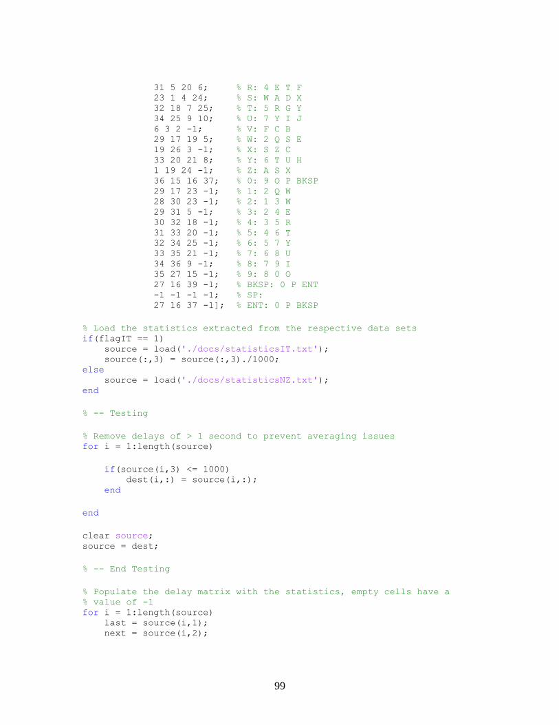
99
31 5 20 6; % R: 4 E T F 23 1 4 24; % S: W A D X 32 18 7 25; % T: 5 R G Y 34 25 9 10; % U: 7 Y I J 6 3 2 -1; % V: F C B 29 17 19 5; % W: 2 Q S E 19 26 3 -1; % X: S Z C 33 20 21 8; % Y: 6 T U H 1 19 24 -1; % Z: A S X 36 15 16 37; % 0: 9 O P BKSP 29 17 23 -1; % 1: 2 Q W 28 30 23 -1; % 2: 1 3 W 29 31 5 -1; % 3: 2 4 E 30 32 18 -1; % 4: 3 5 R 31 33 20 -1; % 5: 4 6 T 32 34 25 -1; % 6: 5 7 Y 33 35 21 -1; % 7: 6 8 U 34 36 9 -1; % 8: 7 9 I 35 27 15 -1; % 9: 8 0 O 27 16 39 -1; % BKSP: 0 P ENT -1 -1 -1 -1; % SP: 27 16 37 -1]; % ENT: 0 P BKSP
% Load the statistics extracted from the respective data sets if(flagIT == 1) source = load('./docs/statisticsIT.txt'); source(:,3) = source(:,3)./1000; else source = load('./docs/statisticsNZ.txt'); end
% -- Testing
% Remove delays of > 1 second to prevent averaging issues for i = 1:length(source)
if(source(i,3) <= 1000) dest(i,:) = source(i,:); end
end
clear source; source = dest;
% -- End Testing
% Populate the delay matrix with the statistics, empty cells have a
% value of -1 for i = 1:length(source) last = source(i,1); next = source(i,2);

100
time = source(i,3);
if(time > 0) delays(last,next) = time; end end
% Back up the original delay matrix for comparison delayOrig = delays;
% Perform multiple passes to fill in as many gaps as possible while (passContinue == 1)
% Keep track of how many passes were made passCounter = passCounter + 1;
% Iterate through the delay matrix to fill gaps for i = 1:39 for j = 1:39
% If there's a gap: if delays(i,j)==-1
% First, attempt interpolating from destination key
% neighbors
% Hold j (destination key) constant, extract the
% neighbor list nList = neighbors(j,:); nPos = 1; count = 0; delayTemp = 0;
% Iterate over known neighbors while (nPos < 5 && nList(nPos) > 0) if(delays(i,nList(nPos)) > 0) delayTemp = delayTemp + delays(i,nList(nPos)); count = count + 1; end nPos = nPos + 1; end
% Average the delay, if values were available if(count > 0) delays(i,j) = delayTemp ./ count; end
% If the value is still negative (a gap), attempt
%interpolation from source key neighbors if delays(i,j)==-1
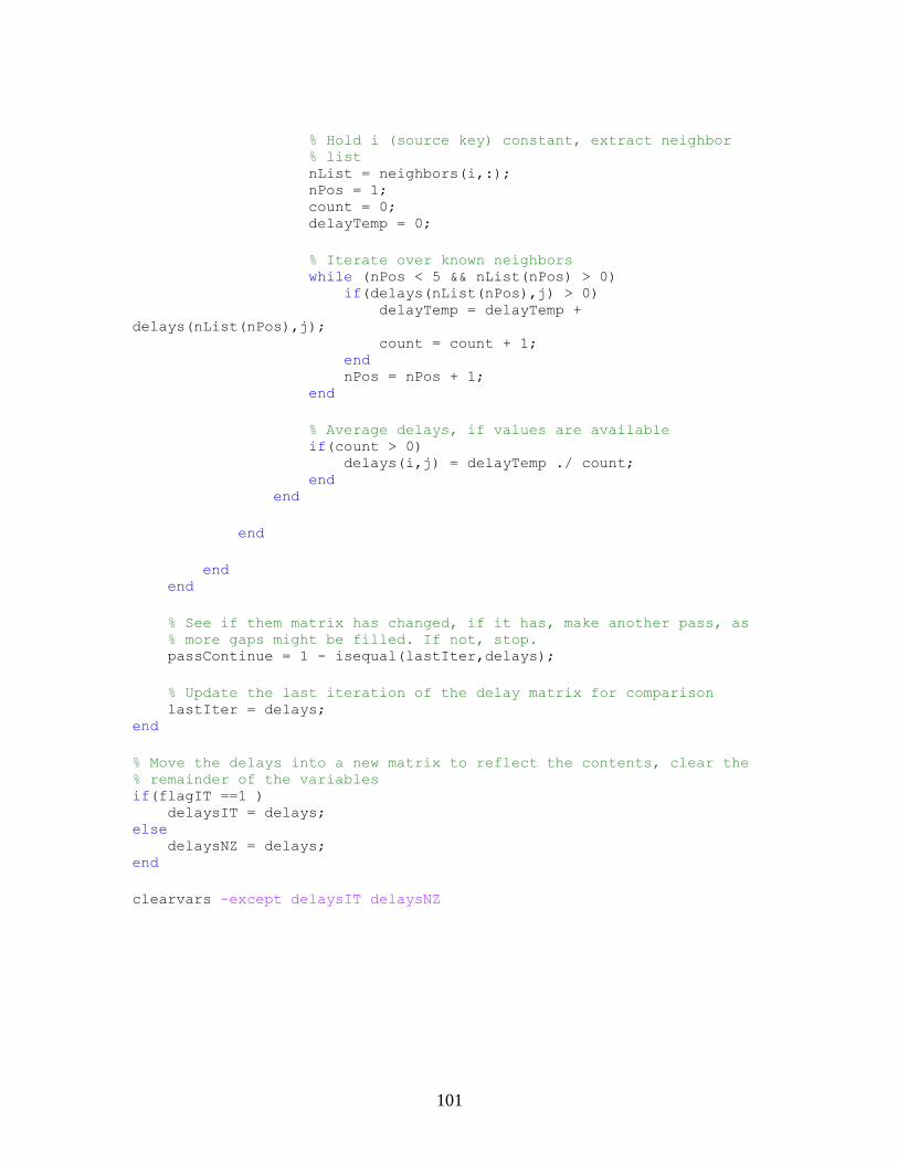
101
% Hold i (source key) constant, extract neighbor
% list nList = neighbors(i,:); nPos = 1; count = 0; delayTemp = 0;
% Iterate over known neighbors while (nPos < 5 && nList(nPos) > 0) if(delays(nList(nPos),j) > 0) delayTemp = delayTemp +
delays(nList(nPos),j); count = count + 1; end nPos = nPos + 1; end
% Average delays, if values are available if(count > 0) delays(i,j) = delayTemp ./ count; end end
end
end end
% See if them matrix has changed, if it has, make another pass, as
% more gaps might be filled. If not, stop. passContinue = 1 - isequal(lastIter,delays);
% Update the last iteration of the delay matrix for comparison lastIter = delays; end
% Move the delays into a new matrix to reflect the contents, clear the % remainder of the variables if(flagIT ==1 ) delaysIT = delays; else delaysNZ = delays; end
clearvars -except delaysIT delaysNZ

102
% digraphTimes.m % % Created: 11/30/2009 (c) Harikrishnan Bhanu % Updated: 12/13/2009 % % Loads the Matlab Data file 'digraphtimes.mat', containing the data % extracted from 'digraphtimes.csv'. It then translates the keypair
% data into the format used in our delay matrix.
% Load the data ('data' and 'textdata') load('digraphtimes.mat');
delaySum = zeros(39,39); freqCount = zeros(39,39);
% Break apart the source and destionation keys % % '110 82' -> 65,41 (as integers, then divided by 2 to convert to
% ASCII) for i=1:length(textdata)
% Search the first column of the csv (stored as textdata) for the
% space separating the source and destination keys spPos = cell2mat(strfind(textdata(i),' ')); str = cell2mat(textdata(i)); lastStr = str(1:spPos(1)-1); nextStr = str(spPos(1)+1:length(str));
% Convert from strings to integers, then divide by 2 to convert to % ASCII value last = str2num(lastStr)/2; next = str2num(nextStr)/2;
% Replace the ASCII values with the corresponding indices for the
% 39x39 matrix (and ensure only appropriate characters are
% considered) if (last > 64 && last < 90) last = last - 64; elseif (last > 47 && last < 58) last = last - 47 + 26; elseif (last == 8) last = 37; elseif (last == 32) last = 38; elseif (last == 13) last = 39; else last = -1; end
if (next > 64 && next < 90) next = next - 64;

103
elseif (next > 47 && next < 58) next = next - 47 + 26; elseif (next == 8) next = 37; elseif (next == 32) next = 38; elseif (next == 13) next = 39; else next = -1; end
% Add the observed delay to the running total for that pair, and % increment the frequency counter if(last ~= -1 && next ~= -1) delaySum(last,next) = delaySum(last,next) + data(i,1); freqCount(last,next) = freqCount(last,next) + 1; end end
% Write out the means outFile = fopen('statisticsNZ2.txt','w+'); for i = 1:39 for j = 1:39 if(delaySum(i,j)~=0) % Comptue the means for all delays for which there was
% data, then write them out. fprintf(outFile,'%d %d
%.3f\n',last,next,delaySum(i,j)/freqCount(i,j)); end end end fclose(outFile);

104
% proximity.m % % Created: 11/24/2009 (c) Harikrishnan Bhanu % Updated: 12/03/2009 % % Determines the locations of keypairs where the delays are too close
% for distinction, between the New Zealand and Italian data.
% Determine the degree of separation between the matricies diff = abs(delaysNZ - delaysIT);
% Create a proximity matrix % distance(i,j) = 1 if diff(i,j) < 15, else distance(i,j) = 0 % % This is basically a boolean matrix determining if the difference % between the Italian and New Zealand data is less than 15ms distance = zeros(39,39);
% Coompare elements and identify those whose delays are too close for i = 1:39 for j = 1:39
if( diff(i,j) < 15 )
distance(i,j) = 1;
end
end end
% Plot the sparsity spy(distance)
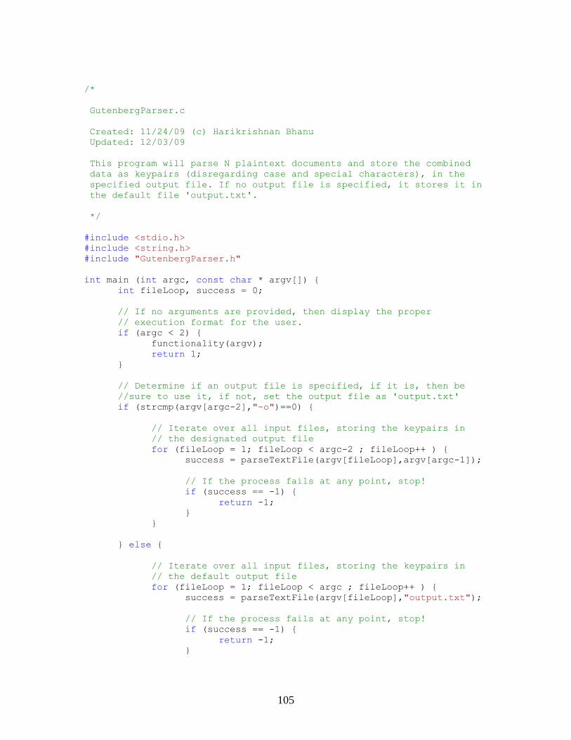
105
/*
GutenbergParser.c
Created: 11/24/09 (c) Harikrishnan Bhanu
Updated: 12/03/09
This program will parse N plaintext documents and store the combined
data as keypairs (disregarding case and special characters), in the
specified output file. If no output file is specified, it stores it in
the default file 'output.txt'.
*/
#include <stdio.h>
#include <string.h>
#include "GutenbergParser.h"
int main (int argc, const char * argv[]) {
int fileLoop, success = 0;
// If no arguments are provided, then display the proper
// execution format for the user.
if (argc < 2) {
functionality(argv);
return 1;
}
// Determine if an output file is specified, if it is, then be
//sure to use it, if not, set the output file as 'output.txt'
if (strcmp(argv[argc-2],"-o")==0) {
// Iterate over all input files, storing the keypairs in
// the designated output file
for (fileLoop = 1; fileLoop < argc-2 ; fileLoop++ ) {
success = parseTextFile(argv[fileLoop],argv[argc-1]);
// If the process fails at any point, stop!
if (success == -1) {
return -1;
}
}
} else {
// Iterate over all input files, storing the keypairs in
// the default output file
for (fileLoop = 1; fileLoop < argc ; fileLoop++ ) {
success = parseTextFile(argv[fileLoop],"output.txt");
// If the process fails at any point, stop!
if (success == -1) {
return -1;
}

106
}
}
return 0;
}

107
/*
GutenbergParser.h
Created: 11/24/09 (c) Harikrishnan Bhanu
Updated: 12/03/09
Header for GutenbergParser.c containing functions.
*/
/*
Function: functionality
Inputs: const char* argv[]
Outputs: none
Displays the proper syntax to run the parser application.
*/
void functionality(const char* argv[]) {
printf("%s input1 [input2] [input3] ... [inputN] [-o
output]\n",argv[0]);
printf(" input* - plaintext file containing text to be
parsed\n");
printf(" at least one is required\n");
printf(" [output] - default output, output.txt, is used
unless\n");
printf(" other filename is specified using the -o
flag\n");
}
/*
Function: parseTextFile
Inputs: const char* inFile - string containing source file name
const char* outFile - string containing destination file
name
Outputs: integer representation of success, a -1 is failure while 0
is success
Parses text from the file pointed to by inFile, removes case (by
forcing all text into upper-case) and all special characters. Then,
puts the contents into the file pointed to by outFile in pairs (comma
separated), each on its own line.
Ex:
"And" --> "1,14" \n "14,4" \n
*/
int parseTextFile(const char* inFile, const char* outFile) {
// Display informational text
printf("Attempting parse from [ %s ].\n",inFile);

108
printf("Destination file [ %s ].\n",outFile);
// Current character from source file stream, as well as the pair
// (last,next) to be written to the destination file stream.
char current, last, next, temp;
// Open the source and destination files. Source is kept read-
// only while the destination file is opened in appending mode.
FILE* source = fopen(inFile, "r");
FILE* dest = fopen(outFile, "a");
// If the source file is unable to be opened, fail gracefully and
// inform the user of the situation.
if (source == NULL) {
printf("Error: Unable to open source file %s.\n",inFile);
printf(" Please ensure the file is in the same
directory as this application.\n");
return -1;
}
// Behave similarly if the destination file is unable to be
// opened.
if (dest == NULL) {
printf("Error: Unable to open destination file
%s.\n",outFile);
printf(" Please ensure the file is in the same
directory as this application,\n");
printf(" and the current user has write-permissions
to it.");
return -1;
}
// Initialize the last and next characters as '-'
current = '-';
last = '-';
next = '-';
// Read a character (priming)
fscanf(source,"%c",¤t);
// Loop while data remains
while (current != '^') {
// Remove case by forcing all lower-case into upper
if (current >= 'a' && current <= 'z') {
temp = current - 32;
} else {
temp = current;
}
// Ensure only appropriate characters are written out

109
if ( (temp >= '0' && temp <= '9') || (temp >= 'A' && temp
<= 'Z') || temp == 10 || temp == 13 || temp == 32) {
// If this is the first character read, then we
// simply store it as 'last' otherwise, we write the
// pair out
if (last=='-') {
last = temp;
}
else {
// If this isn't the first character read, then
// there is a 'last' entry, so this is the
// 'next' entry
next = temp;
int char1,char2;
// Convert to the interger indicies of the
// delay matrix
if(last >= 'A' && last <='Z') {
char1 = last - 64;
} else if (last >= '0' && last <= '9') {
char1 = last - 47 + 26;
} else if (last == 13 || last == 10) {
char1 = 39;
} else {
char1 = 38;
}
if(next >= 'A' && next <='Z') {
char2 = next - 64;
} else if (next >= '0' && next <= '9') {
char2 = next - 47 + 26;
} else if (next == 13 || next == 13) {
char2 = 39;
} else {
char2 = 38;
}
fprintf(dest, "%d,%d\n",char1,char2);
// Update 'last' and reset 'next'
last = next;
next = '-';
}
}
// Read the next character
fscanf(source,"%c",¤t);
}
// Close the file pointers and return to the main program body
printf("Closing [ %s ] and [ %s ].\n",inFile,outFile);

110
fclose(source);
fclose(dest);
return 0;
}

111
% GutenbergDelay.m % % Created: 11/28/2009 (c) Harikrishnan Bhanu % Updated: 12/03/2009 % % Loads the text file 'composite.txt', containing the parsed training
% data stored as keypairs. Then, performs a lookup, using the delays
% matrix generated by delayFill.m, of the interkeystroke delays and
% stores these values in tVal.
% Flag to determine if Italian or English is being considered flagIT = 0;
% Load delay matrices load('proximity.mat');
% Load the keypairs pulled from the text by the parser, load the bounds
% for the symbolization, and then open the file for writing if (flagIT == 1) pairs = load('./Italian/composite.txt'); bounds = load('it.tsl'); outFile = fopen('ITSym.csv','w+'); delays = delaysIT; else pairs = load('./English/composite.txt'); bounds = load('nz.tsl'); outFile = fopen('NZSym.csv','w+'); delays = delaysNZ; end tVal = zeros(length(pairs),1);
% Scale from seconds to milliseconds bounds = bounds .* 1000;
% Conver to delays for i = 1:length(pairs) tVal(i) = delays(pairs(i,1),pairs(i,2)); end
% Symbolize the time values and write them to a CSV for i=1:length(tVal)
% Where does this delay fall? match = 0; q = 1; while(match ~= 1) if (ceil(tVal(i)) >= bounds(q,1) && ceil(tVal(i)) <=
bounds(q,2)) match = 1; else q = q + 1; end

112
end
% Define the symbol associated with that position symbol = char(65+q);
% Then write the symbol to the file if i<length(tVal) %fprintf(outFile,'%c,',symbol); fprintf(outFile,'%.3f\n',tVal(i)); else %fprintf(outFile,'%c',symbol); fprintf(outFile,'%.3f\n',tVal(i)); end
end
% Close the file fclose(outFile);

113
% gNG.m % % Created: 11/04/2008 (c) Harikrishnan Bhanu % Updated: 12/03/2009 % % Growing neural gas code originally written for ECE872, modified to
% locate clusters within interkeystroke delay sets. Source data is
% stored in H, resulting cluster values are stored in A.
N = 2; % Initialize size of A H = NZ1D'; % Specify data source to search for
% clusters [Hsize , dimensions] = size(H); % Number of training vectors and their
% dimensions
% Initialize the set of vectors as d x N, where d is the dimension of
% the vectors and N is the number of initial units, 2
% A Gaussian distribution is used here with a mean of 0 and standard % deviation of 10 A = sqrt(10)*randn(N,dimensions);
% Initialize connection ages as -1, for not formed and change diagonal % entries to -2, denoting it is the same unit to itself, 0 denotes a
% new connection, and an age greater than zero is how many iterations
% that conneciton has gone without change C = -1 * ones(N,N); for i=1:N C(i,i) = -2; end
% Error matrix -- how well current units represent the data set, % initialized to zeros E = zeros(N,1);
% Max number of presentations that an edge is allowed a_max = 10;
% Max number of presentations allowed p_max = 1000000;
% Error decay rate for unit creation alpha = 0.5;
% Error decay for all units, per presentation d = 0.9995;
% Presentation limit before new unit can be added lambda = 1000;
% Presentation number, initialized to 0 k = 0;
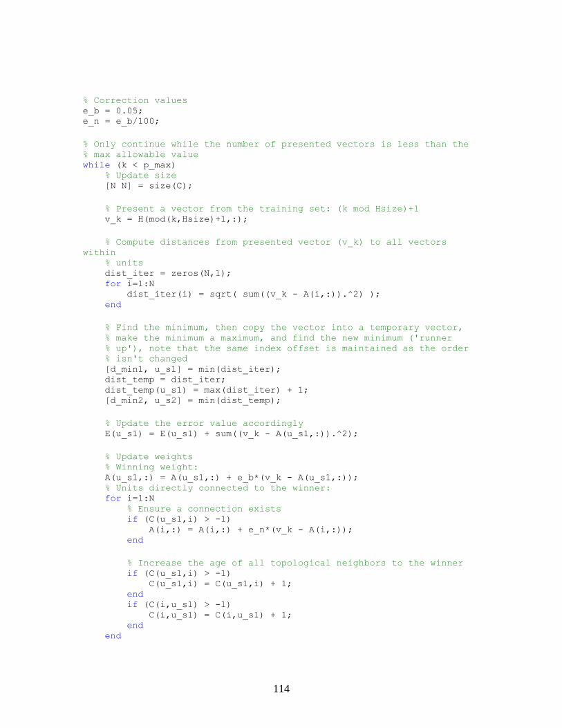
114
% Correction values e_b = 0.05; e_n = e_b/100;
% Only continue while the number of presented vectors is less than the
% max allowable value while (k < p_max) % Update size [N N] = size(C);
% Present a vector from the training set: (k mod Hsize)+1 v_k = H(mod(k,Hsize)+1,:);
% Compute distances from presented vector (v_k) to all vectors
within % units dist_iter = zeros(N,1); for i=1:N dist_iter(i) = sqrt( sum((v_k - A(i,:)).^2) ); end
% Find the minimum, then copy the vector into a temporary vector, % make the minimum a maximum, and find the new minimum ('runner
% up'), note that the same index offset is maintained as the order
% isn't changed [d_min1, u_s1] = min(dist_iter); dist_temp = dist_iter; dist_temp(u_s1) = max(dist_iter) + 1; [d_min2, u_s2] = min(dist_temp);
% Update the error value accordingly E(u_s1) = E(u_s1) + sum((v_k - A(u_s1,:)).^2);
% Update weights % Winning weight: A(u_s1,:) = A(u_s1,:) + e_b*(v_k - A(u_s1,:)); % Units directly connected to the winner: for i=1:N % Ensure a connection exists if (C(u_s1,i) > -1) A(i,:) = A(i,:) + e_n*(v_k - A(i,:)); end
% Increase the age of all topological neighbors to the winner if (C(u_s1,i) > -1) C(u_s1,i) = C(u_s1,i) + 1; end if (C(i,u_s1) > -1) C(i,u_s1) = C(i,u_s1) + 1; end end

115
% Does a connection exist between the winner and runner up? If not, % make one. C(u_s1,u_s2) = 0; C(u_s2,u_s1) = 0;
% Pass through connection matrix and trim any vectors which haven't % been updated within a_max presentations for i=1:N for j=1:N if(C(i,j) > a_max) C(i,j) = -1; end end end
% Remove any units which have no connections [N N] = size(C); prune = ones(N,1); for i=1:N for j=1:N if(C(i,j) > -1) prune(j) = 0; end end end for i=N:-1:1 % Only prune if no connections if(prune(i)==1) C(i,:) = []; % Row -- overwrite to the top C(:,i) = []; % Column -- overwrite to the left A(i,:) = []; % Remove the unit itself E(i,:) = []; % Remove the error associated with the unit end end
[N N] = size(C);
% Add a new unit % Is k an integer multiple of lambda? if (mod(k,lambda)==0) % Find the one unit who has the most 'errors' [q_val, u_q] = max(E);
% Find the unit which is connected to u_q directly, with the
most % 'errors' E_temp = -1*ones(N,1); for i=1:N if(C(u_q,i) > -1) E_temp(i) = E(i); end

116
end [f_val, u_f] = max(E_temp);
% New weight is between u_q and u_f w_r = .5.*(A(u_q,:) + A(u_f,:)); % Remove edge between u_q & u_f C(u_q,u_f) = -1; C(u_f,u_q) = -1; % Insert u_r between u_q and u_f % Shift over existing units u_r = min(u_q,u_f)+ceil(abs((u_q - u_f))/2); C_temp = -1*ones(N+1,N+1); for i=1:N % 'Left' Half if(i < u_r) for j=1:N % 'Left Top' -- direct copy if(j < u_r) C_temp(i,j) = C(i,j); end % 'Left Bottom' -- shifted 1 down if(j >= u_r) C_temp(i,j+1) = C(i,j); end end A(i,:) = A(i,:); E(i) = E(i); end
% 'Right' Half if(i >= u_r) for j=1:N % 'Right Top' -- shifted 1 right if(j < u_r) C_temp(i+1,j) = C(i,j); end % 'Right Bottom' -- shifted 1 right, 1 down if(j >= u_r) C_temp(i+1,j+1) = C(i,j); end end A(i+1,:) = A(i,:); E(i+1) = E(i); end end clear C; C = C_temp; [N N] = size(C);
for i=1:N C(u_r,i) = -1; C(i,u_r) = -1; end
117
% Insert the vector A(u_r,:) = w_r; if(u_f >= u_r) C(u_r,u_q) = 0; % r -> q C(u_r,u_f+1) = 0; % r -> f C(u_q,u_r) = 0; % q -> r C(u_f+1,u_r) = 0; % f -> r else C(u_r,u_q+1) = 0; % r -> q C(u_r,u_f) = 0; % r -> f C(u_q+1,u_r) = 0; % q -> r C(u_f,u_r) = 0; % f -> r end
% Update error for u_r, u_f & u_q E(u_f) = E(u_f) + alpha * E(u_f); E(u_q) = E(u_q) + alpha * E(u_q); E(u_r) = E(u_q); end
% Update error, presentation value, and ensure that -2 line the % diagonal E = (1-d).*E; k = k+1; [N N] = size(C); for i=1:N C(i,i) = -2; end end

118
% keyGaussPlot.m % % Created: 12/07/09 % Updated: 12/08/09 % % Opens a specified document containing keypair statistics for a given % language (Italian or English, in this case). It then plots Gaussian % distributions for all keypairs that appear with more frequency than
% the specified threshold.
% Specify language flagIT = 1;
% Specify frequency threshold threshold = 200;
% Initialize counter to 0 pairs = 0;
% Open the corresponding language statistics file % Note: Interpolated data is NOT considered, only original data % Note: The filename is 'fullStatistics*', as opposed to 'statistics*'
% to differentiate between the two. if(flagIT == 1) % Open IT statistics document data = load('./docs/fullStatisticsIT.txt'); else % Open NZ statistics document data = load('./docs/fullStatisticsNZ.txt'); end
% Set the time scale -- 10 ms increments from 0 to 1000 ms t = 0:1:100;
% Scale from microseconds to milliseconds for the Italian data if(flagIT == 1) data(:,3) = data(:,3) / 1000; end
% Go through the data to determine what should be plotted, and plot
% them for i = 1:length(data)
% Ensure that the threshold is met and outlier data isn't processed % ( > 800 ms delays) if(data(i,5) >= threshold && data(i,3) < 800) % Increment counter pairs = pairs + 1;
% Extract the mean and variance, then take the square root of
% the variance to get the standard deviation mVal = data(i,3);
119
vVal = data(i,4); sVal = sqrt(vVal); plot(0:1:100,gaussmf(t,[sVal mVal])); hold on; end
end
% Add labels to the graph if(flagIT == 1) str = sprintf('Interkeystroke Gaussians (Italian, greater than %d
samples)\n%d Pairs',threshold,pairs); else str = sprintf('Interkeystroke Gaussians (New Zealand, greater than
%d samples)\n%d Pairs',threshold,pairs); end xlabel('Delays (seconds)'); title(str);

120
% roc.m % % Created: 2/26/10 (c) Harikrishnan Bhanu % Changed: 2/26/10 % % Plots RoC curves for the confidence interval (CI) and forward-
backward % (FB) data files for English and Italian.
clear;clc;
% Load all four files load('roc.mat');
% Flags to indicate which data file to use italian = 0; confidence = 1;
% Move the selected file if(italian==0) if(confidence==0) % Consider forward-backwards with texts being presented to the % English model truedata = englishFB(1:401); falsedata = italianFB(1:401); else % Consider confidence intervals with texts being presented to
the % English model truedata = englishCI(1:401); falsedata = italianCI(1:401); end else if(confidence==0) % Consider forward-backwards with texts being presented to the % Italian model truedata = italianFB(402:802); falsedata = englishFB(402:802); else % Consider confidence intervals with texts being presented to
the % Italian model truedata = italianCI(402:802); falsedata = englishCI(402:802); end end
% Threshold ranges from 0 to 1 in increments of 0.01 x = [0 : 0.01 : 1]; stats = zeros(4,length(x)); y = zeros(length(x),2);

121
for threshold = 1:length(x)
% Clear true and false classification counters truePos = 0; trueNeg = 0; falsePos = 0; falseNeg = 0;
% Count the true and false positives and negatives for j = 1:401 % Scale against the max available if truedata(j) > (x(threshold)*max(truedata)) truePos = truePos + 1; else falseNeg = falseNeg + 1; end
if falsedata(j) > (x(threshold)*max(truedata)) falsePos = falsePos + 1; else trueNeg = trueNeg + 1; end end
% Store statistics for this threshold stats(:,threshold) = [ truePos ; falsePos ; trueNeg ; falseNeg ]; y(threshold,:) = [truePos/(truePos+falseNeg)
trueNeg/(trueNeg+falsePos)]; end
% Get coordinates to plot xroc=[1; 1-y(:,2); 0]; yroc=[1; y(:,1); 0];
% Plot it plot(xroc,yroc,'r.-')

122
REFERENCES

123
[1] L. E. Baum, T. Petrie, G. Soules, and N. Weiss, "A Mazimization Technique
Occurring in the Statistical Analysis of Probabilistic Functions of Markov Chains,"
The Annals of Mathematical Statistics, vol. 41, no. 1, pp. 164-171, Feb. 1970,
http://www.jstor.org/stable/2239727.
[2] H. Bhanu, et al., "Language Detection over Tunneled Sessions," IEEE Transactions
on SMC, Under Review.
[3] H. Bhanu, J. M. Schwier, C. Griffin, and R. R. Brooks, "Zero-Knowledge Hidden
Markov Model Learning of Tunneled Protocols," IEEE Transactions on SMC, Under
Review.
[4] R. R. Brooks, J. M. Schwier, and C. Griffin, "Behavior Detection using Confidence
Intervals of Hidden Markov Models," IEEE Transactions on SMC Part B, pp. 1484-
92, Dec. 2009.
[5] S. A. Crosby, D. S. Wallach, and R. H. Reidi, "Opportunities and Limits of Remote
Timing Attacks," ACM Transactions on Information and System Security, vol. 12,
no. 3, pp. 1-29, Jan. 2009.
[6] B. Elign and B. Einhorn. (2006, Jan.) The Great Firewall of China. [Online].
http://www.businessweek.com/technology/content/jan2006/tc20060112_434051.htm
[7] E. English and S. Hamilton, "Network Security Under Siege: The Timing Attack,"
IEEE Computer, vol. 29, no. 3, pp. 95-97, Mar. 1996.
[8] D. Gunetti and C. Picardi, "Keystroke Analysis of free Text," ACM Transactions on
Information and System Security, vol. 8, no. 3, pp. 312-347, 2005.
[9] K. Hempstalk, "Continious Typist Verification using Machine Learning," Ph.D.
Dissertation, Department of Computer Science, University of Waikato, Hamilton,
New Zealand, 2009.
[10] J. Ilonen, "Keystroke Dynamics," Advanced Topics in Information Processing -
Lecture., 2003, http://www.it.lut.fi/kurssit/03-04/010970000/seminars/Ilonen.pdf.
[11] T. Kohno, A. Broido, and K. C. Claffy, "Remote Physical Device Fingerprinting,"
IEEE Transactions on Dependable and Secure Computing, vol. 2, no. 2, pp. 211-225,
Apr. 2005.
[12] D. Kravets. (2007, Oct.) RIAA Jury Finds Minnesota Woman Liable for Piracy,
Awards $222,000. [Online]. http://www.wired.com/threatlevel/2007/10/riaa-jury-
finds/

124
[13] F. Monrose and A. D. Rubin, "Keystroke Dynamics as a Biometric for
Authentication," Future Generation Computer Systems, vol. 16, pp. 351-359, 2000.
[14] L. R. Rabiner, "A Tutorial on Hidden Markov Models and Selected Applications in
Speech Recognition," Proceedings of the IEEE, pp. 257-286, Feb. 1989.
[15] J. A. Robinson, V. M. Liang, J. A. M. Chambers, and C. L. MacKenzie, "Computer
User Verification Using Login String Keystroke Dynamics," IEEE Transactions on
SMC - Part A, vol. 28, no. 2, pp. 236-241, Mar. 1998.
[16] J. Schwier, "Pattern Recognition in Command and Control Data Systems," Ph.D.
Dissertation, Holcombe Department of Electrical and Computer Engineering,
Clemson University, Clemson, SC, 2009.
[17] C. R. Shalizi, K. L. Shalizi, and J. P. Crutchfield, "An Algorithm for Pattern
Discovery in Time Series," The Computing Research Repository, Oct. 2002,
cs.LG/021005: http://arxiv.org/abs/cs.LG/021005.
[18] C. R. Shalizi and K. L. Klinkner, Uncertainty in Artificial Intelligence: Proceedings
of the Twentieth Conference (UAI 2004), M. C. a. J. Y. Halpern, Ed. Arlington,
Virginia, USA: AUAI Press, 2004.
[19] R. Sicilano. (2010, Mar.) Biggest Botnet Goes Bust. [Online].
http://www.bloggernews.net/124012
[20] D. X. Song, D. Wagner, and X. Tian, "Timing Analysis of Keystrokes and Timing
Attacks on SSH," SSYM'01: Proceedings of the 10th conference on USENIX Security
Symposium, p. 25, 2001.
[21] R. Taylor. (2006, Jan.) The great firewall of China. [Online].
http://news.bbc.co.uk/2/hi/programmes/click_online/4587622.stm