timing small versus large stocks -...

FALL 2007 THE JOURNAL OF PORTFOLIO MANAGEMENT 41

Ever since Fama and French [1992] published theirseminal work, it has been widely accepted thatsmall stocks should yield a higher return on averagethan large ones. One key point to remember is

that this conclusion holds only on average, and not all the time.A small-size tilt is profitable in the long run, butcan be detrimental for performance over medium-termperiods.The Fama-French small-minus-big (SMB hereafter)U.S. premium over July 1926-June 2005 was 1) negative for 45 of the 75 five-year rolling periods,and 2) positive justa little over half of the time (50.84%). Such observationspave the way for an investigation into when it is preferableto hold large rather than small stocks, and vice versa.

Using ex post data,Reinganum [1999] and Ahmed,Lockwood, and Nanda [2002] document potential papergains to be derived from size-timing strategies. Kester[1990] estimates the transaction costs from such size-timingstrategies, and shows that profitability would hold evenafter reasonable transaction costs.

Most studies examining size timing on an ex antebasis are based on parametric estimation methods. In theU.K., Levis and Liodakis [1999] propose a size-timingapproach for the SMB premium that relies on multivariateordinary least squares (OLS) and logit regressions. Bothrecursive out-of-sample forecast models (repeated annu-ally) use lagged macroeconomic data.They outperform abuy-and-hold benchmark over the 1974-1997 periodeven after accounting for transaction costs.

More recently, in the U.S., Cooper, Gulen, and Vassalou [2001] test recursive OLS models (repeatedmonthly) using filter rules and long-short size deciles overthe out-of-sample 1963-1998 period.They find evidenceof size-timing strategies.

Timing Small versus Large StocksUsing artificial intelligence to decide when to be long or short.

Jean-François L’Her, Tammam Mouakhar, and Mathieu Roberge

JEAN-FRANÇOIS L’HER

is a senior vice president,Investment PolicyResearch, at the Caisse deDépôt et Placement duQuébec in Montré[email protected]

TAMMAM MOUAKHAR

is a research advisor at theCaisse de Dépôt et Placement du Qué[email protected]

MATHIEU ROBERGE

is a research advisor at theCaisse de Dépôt et Placement du Qué[email protected]

IT IS

ILLEGAL T

O REPRODUCE T

HIS A

RTICLE IN

ANY F

ORMAT

Copyright © 2007

42 TIMING SMALL VERSUS LARGE STOCKS FALL 2007

In the same vein,Amenc et al. [2003] test recursiveOLS models using real indexes over an out-of-sample2000-2002 period.They also document profitable size-timing strategies.

These parametric methods have the advantage ofusing parsimonious models that clearly identify functionalforms and the marginal contribution of each variable,butthey also suffer from several flaws—restrictive distribu-tion assumptions, linear functional forms, and sensitivityto outliers. Size-timing is a good candidate for non-parametric methods because even if there were evidenceof the predictive power of lagged macroeconomic vari-ables,we do not have a priori hypotheses on the variablesand on the functional form of the relation.

To our knowledge, there is only one application of a non-parametric style-timing method—Kao and Shumaker [1999] build a successful value-growth timingmodel based on a recursive partitioning algorithm.

We focus mainly on comparing the predictive powerof different approaches based on artificial intelligence (AI)with respect to the size-timing problem.We compare theability of recursive partitioning (RP), neural networks(NNs), and genetic algorithm (GA) approaches to cor-rectly time the size premium, and examine the resultingperformance.We also examine the predictive power aswell as the performance of a strategy based on a consensusof the three approaches.

METHODS

Three popular AI models, recursive partitioning,neural networks, and genetic algorithms, are initiallytrained during an in-sample period from January 1975through December 1989.Out-of-sample predictive powerand investment performance are then assessed for January1990-December 2004.

Advantages and Disadvantages of AI Methods

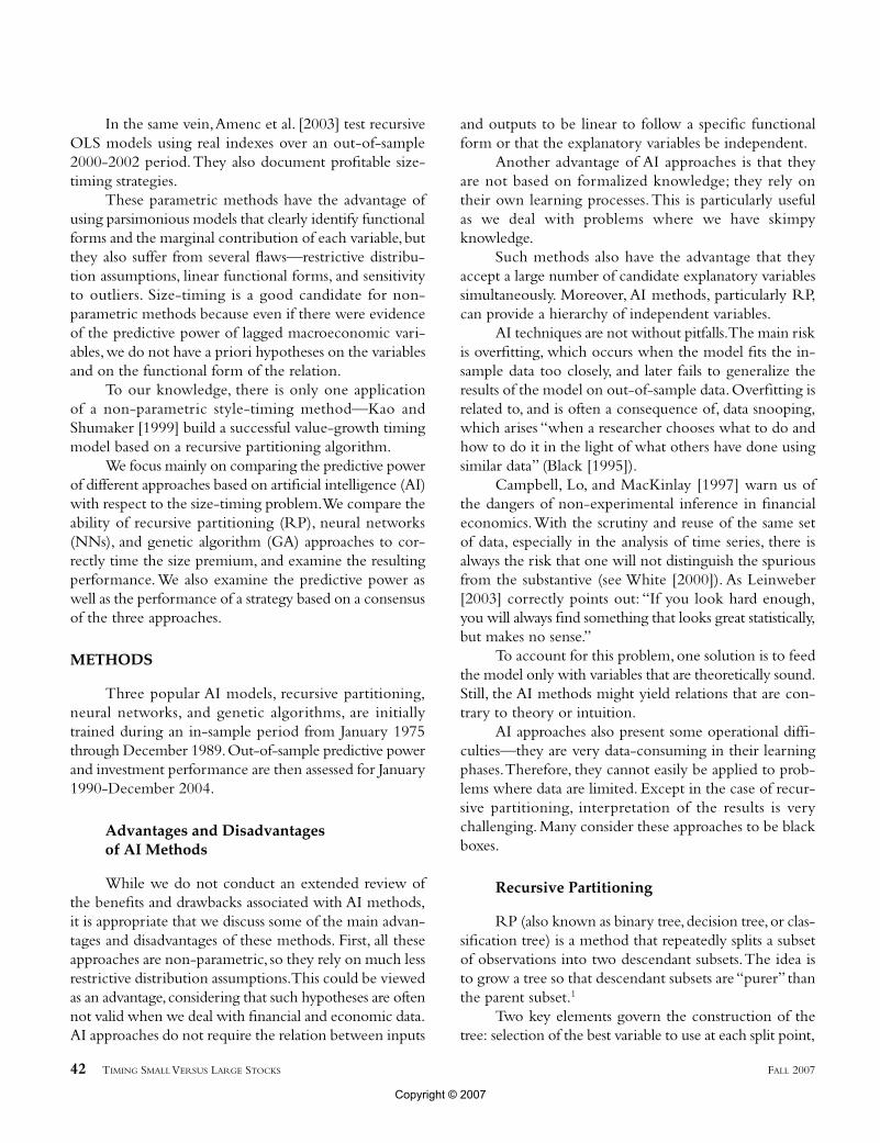
While we do not conduct an extended review ofthe benefits and drawbacks associated with AI methods,it is appropriate that we discuss some of the main advan-tages and disadvantages of these methods. First, all theseapproaches are non-parametric, so they rely on much lessrestrictive distribution assumptions.This could be viewedas an advantage,considering that such hypotheses are oftennot valid when we deal with financial and economic data.AI approaches do not require the relation between inputs

and outputs to be linear to follow a specific functionalform or that the explanatory variables be independent.

Another advantage of AI approaches is that they are not based on formalized knowledge; they rely on their own learning processes.This is particularly useful as we deal with problems where we have skimpy knowledge.

Such methods also have the advantage that theyaccept a large number of candidate explanatory variablessimultaneously. Moreover, AI methods, particularly RP,can provide a hierarchy of independent variables.

AI techniques are not without pitfalls.The main riskis overfitting, which occurs when the model fits the in-sample data too closely, and later fails to generalize theresults of the model on out-of-sample data.Overfitting isrelated to, and is often a consequence of, data snooping,which arises “when a researcher chooses what to do andhow to do it in the light of what others have done usingsimilar data” (Black [1995]).

Campbell, Lo, and MacKinlay [1997] warn us of the dangers of non-experimental inference in financialeconomics.With the scrutiny and reuse of the same setof data, especially in the analysis of time series, there isalways the risk that one will not distinguish the spuriousfrom the substantive (see White [2000]). As Leinweber[2003] correctly points out: “If you look hard enough,you will always find something that looks great statistically,but makes no sense.”

To account for this problem,one solution is to feedthe model only with variables that are theoretically sound.Still, the AI methods might yield relations that are con-trary to theory or intuition.

AI approaches also present some operational diffi-culties—they are very data-consuming in their learningphases.Therefore, they cannot easily be applied to prob-lems where data are limited. Except in the case of recur-sive partitioning, interpretation of the results is verychallenging. Many consider these approaches to be blackboxes.

Recursive Partitioning

RP (also known as binary tree,decision tree,or clas-sification tree) is a method that repeatedly splits a subsetof observations into two descendant subsets.The idea isto grow a tree so that descendant subsets are “purer” thanthe parent subset.1

Two key elements govern the construction of thetree: selection of the best variable to use at each split point,

Copyright © 2007

and choice of a criterion that lets us determine when tostop splitting (hence creating a terminal node) or whento split further. Criteria such as a minimal number ofobservations in each terminal node or a minimum levelof purity are typically used to determine whether a nodeshould be split further. Once the tree has been built, allterminal nodes are assumed to classify an observationaccording to the outcome most frequently encounteredat that node.

A more detailed description can be found in Breimanet al. [1984].Additional information on specific applica-tions to finance appears in Kao and Shumaker [1999] andSorensen, Miller, and Ooi [2000].

For our particular application, numerous tree con-figurations are tested in an attempt to maximize the in-sample hit rate (measured as the number of correctpredictions divided by the total number of predictionsmade).A constraint forces all trees to grow in such a fashionthat at least ten observations end up in any single terminalnode.This constraint is enforced in an effort to minimizethe risk of overfitting.

The Gini diversity index is used to determine thebest split at each step. No prior probabilities are used.

Neural Networks

An artificial neural network uses a set of conceptsbased on the biological neural system. It is composed ofartificial neural nodes (or processing elements) intercon-nected in a way that allows parallel processing.Each nodereceives an input signal, processes the input through atransfer function, and transforms it into an output.

The NN architecture is flexible, and is characterizedby the number of layers, the number of neurons in eachlayer, the interconnection between the neurons, and thetransfer function of each neuron.The multiple-layer struc-ture is composed of an input layer (the first layer whereexternal inputs are received), the hidden layer (which canconsist of one or more intermediate layers), and the outputlayer (the last layer, which delivers the output).All nodesin each preceding layer are connected to the next layer by arcs.

In order to process the output, NNs need to betrained.The process of training (or learning) consists ofadjusting the parameters (the arc weights) of the neural network model by minimizing the differencebetween the NN output and the known in-sample targetaccording to a learning algorithm. Once the NN hasbeen trained on the in-sample set, it is applied to an

out-of-sample set in order to evaluate the predictive capa-bility of the model.

A more complete description of this method canbe found in Medsker, Trippi, and Turban [1993].Kryzanowski,Galler, and Wright [1993] and Kingdon andFeldman [1995b] present interesting applications tofinance.

To determine the structure of our NN, the learningperiod is subdivided into two subperiods.Different struc-tures are trained in the first subperiod (1975-1983).Thetraining phase is conducted in order to minimize the dif-ference between the NN monthly outputs and the asso-ciated actual in-sample return.Models are then tested onthe second subperiod (1984-1989).

The model that is selected to be applied to the out-of-sample set is the one that minimizes the mean squarederrors between the NN outputs and the 1984-1989 in-sample returns.

Genetic Algorithms

A genetic algorithm is a stochastic search techniquethat is based on the theories of natural selection andgenetics, and is designed to optimize a fitness function.The approach randomly generates a set of potential solu-tions.The set is known as the population, and each poten-tial solution is called an individual. Each individual, alsocalled a chromosome by some, is represented by a codifiedbinary vector.

The GA first evaluates the fitness function for eachindividual in the population, and then the processes ofnatural selection, reproduction (cross-over), and mutationoperate to make the population evolve to the next gen-eration.The process goes on until a predetermined stop-ping criterion is reached.Typical stopping criteria includereaching a fixed number of generations or a targetedhomogeneity in the population.

Natural selection is the process through which indi-viduals with the highest fitness are automatically retainedin the newly generated population (these individuals arecloned). Cross-over is the operation through which twoindividuals are mixed in an attempt to obtain a new indi-vidual with better fitness than that of both its parents.Finally, mutation represents a rare and random innova-tion in the binary sequence of an individual.

The main challenge in GA is defining an appro-priate fitness function. GAs are very flexible, and providemany parameters that can be calibrated to better fit theproblem under study.


Copyright © 2007

For further details, see Bauer [1994]. Kingdon andFeldman [1995a] provide a good example of how GAcould be applied to finance.

For our size-timing application, we specify theproblem as a linear function of 20 variables such that:

V1 through V20 correspond to the values taken bythe different predictive values at any date, and β1 throughβ20 as well as π are values optimized by the genetic oper-ators such as reproduction and mutation. β1 through β20

and π are optimized to maximize the in-sample return.We use a population size of 100 individuals and a fixednumber of 100 generations as stopping criteria.The chro-mosomes are long binary strings representing the 20parameters to be optimized in the equation.

The translation into and back from the binary rep-resentation is conducted automatically by Matlab.The fit-ness function evaluated with each chromosome ismaximization of the return obtained when applying therule depicted in the equation to the in-sample period.Reproduction is performed with an elite count of tenand a cross-over fraction of 0.8.2

APPLICATION

Many authors suggest that the positive small-minus-big premium is related to the fundamental risk in theeconomy (see Fama and French [1993,1996] and Jensen,Johnson, and Mercer [1998]).They shed light on the linksbetween the fluctuation of the SMB premium and theeconomic cycle. Fama and French [1993, 1996] suggestthat the earnings of small firms could be more sensitiveto economic conditions. Jensen, Johnson, and Mercer[1998] note that the size of the SMB premium is linkedto a tightening of monetary policy.When the Fed raisesinterest rates, monetary policy becomes more restrictiveand the premium narrows. Conversely, they find that theSMB premium widens with a more accommodating mon-etary policy.3

Other authors use lagged macroeconomic variablesto design a style-timing model focusing on size.4 Themacroeconomic variables most frequently used to predict

If V V + V + + V :

Model favors small - cap

If V + V + V + + V :

Model favors large - cap

1 1 2 2 3 3 20 20

1 1 2 2 3 3 20 20

β β β β π

β β β β π

+ >

≤

…

…

the SMB premium are related to interest rates.Variablessuch as term spreads and the level of the short-term rateare used in Levis and Liodakis [1999],Cooper,Gulen, andVassalou [2001], and Amenc et al. [2003].

Variables related to the stock market are also common.Levis and Liodakis [1999], Cooper, Gulen, and Vassalou[2001], and Amenc et al. [2003] use the dividend yield,while Kao and Shumaker [1999] consider the differentialbetween the earnings-to-price ratio of the S&P 500 andthe long-term bond yield. Other authors document thepredictive power of New York Stock Exchange volume,the market premium, and corporate credit.

Some also use classic macroeconomic variables such as GDP growth and inflation. Finally,Amenc et al.[2003] examine more original variables, including com-modity prices, exchange rates, and the level of consumerconfidence.

We use the 20 variables described in Exhibit 1 to feedthe three AI approaches.

Models for the Three Approaches

We first train the three AI approaches over January1975-December 1989.The recursive programming resultsare the easiest to interpret.The RP tree has 28 terminalnodes.The shortest path to a terminal node is two splits,while the longest requires ten splits.Thirteen variables areused as split criteria at least once within the tree struc-ture:CREDIT,TBILL,COIN,LEAD,MOM,DIV,CAP,IND, CSI, ISM, SAV, PPI, and TRAD.The most impor-tant variable (the first split criterion) is the U.S. Confer-ence Board Coincident Economic Indicators Index(COIN).The next split on the left uses the variable DIV,and the next on the right the MOM.5

The NN structure is composed of one hidden layerwith 20 nodes. Its architecture corresponds to the standardneural network architecture for non-linear regression (seeHaykin [1994]). The hidden units use hyperbolic tangent activation functions,and the output unit has a linearactivation function.We use the Levenberg-Marquardt back-propagation algorithm to train the network.Bayesian reg-ularization is implemented in this algorithm to preventoverfitting and to produce a network that can be fullygeneralized.

Interpretation of the NN model is more complex,because the multi-layer structure involves a high degreeof black box.We can only roughly measure the importanceof the different input variables.The most suitable methodfor comparing the relative importance of the variables is


Copyright © 2007

the connection weight approach (see Olden, Joy,and Death[2004]). The results show that INFL, TERM, COIN,EARN, and MOM are the factors that contribute the most.

In the GA approach, the variables TERM, COIN,LEAD, MOM, EARN, DIV, GSCI, CAP, ISM, M2,PPI, NYSE, and TRAD are all associated with a positivecoefficient.6 The seven other variables,CREDIT, TBILL,INFL, IND, CSI, SAV, and CEXP, have negative coeffi-cients. This implies that, ceteris paribus, a positive change in the first set of variables will tend to favor small-caps and a positive change in the second set will favorlarge-caps.

Predictive Ability and Investment Performance

Panel A of Exhibit 2 presents the performance of thethree size-timing strategies over January 1990-December2004.The performance of the classic small-minus-big

strategy is also shown for comparison.Two of the three style-timing strategies (RP and NN) dominate SMB in terms ofreturn per unit of risk,but the third method(GA) fails to time the size premium.

The performance of the two successfultiming strategies in terms of return per unitof risk is driven by average excess returnsthat are more than 400 basis points higher(6.25% for RP and 6.91% for NN versus1.52% for SMB).The three AI timing strate-gies and the SMB are roughly as volatile,with a difference of under 20 basis pointsbetween the highest and the lowest.

The relative performance of timingstrategies is greatly influenced by extremeobservations. Indeed, our timing strategiesimply binary decisions: short or long posi-tions in the small- or large-caps.Therefore,making the wrong decision in a givenmonth can convert a wonderful month intoa nightmarish one, and vice versa. Thehighest absolute value of the SMB is seenin February 2000 (21.49%). This atypicalobservation translates into a maximummonthly gain for the RP and NN timingstrategies, but turns into a maximum lossfor the GA.

Another way to analyze the perform-ance of the three AI approaches is to compare their hitrates,which show if a predictive model is right on average.A high rate with a disappointing return implies that a fewwrong decisions hurt much more than the more frequentgood decisions helped. In this case, a poor return mightsimply be due to misfortune.This could be the case for the GA timing model, which posts a satisfying hit rate of 54.4%,higher than the SMB hit rate of 52.8%.The RPand NN approaches reach higher hit rates of 56.1% and 57.0%.

All results so far are obtained by training the differentAI approaches on a static learning sample.That is, as wemove along the test sample (out-of-sample), new predic-tions do not take into account the newest information avail-able, and are not based on recent available data. It seemslogical to examine whether expandable learning samplescould improve prediction.We thus reexamine timing strate-gies trained on expandable learning samples, or dynamicstrategies. This idea corresponds to the concept of an


E X H I B I T 1Variables Used For Size-Timing

Copyright © 2007

evolving tree, as discussed in Sorensen, Miller, and Ooi[2000].

In our case,we let the AI models evolve at the begin-ning of each year rather than each month.Therefore, eachpredictive model is used to make 12 monthly predictionsbefore it is updated.The results for evolving predictivemodels are presented in Exhibit 3.

Only one method, the genetic algorithm, yieldsbetter results with an expandable learning sample.Thereturn associated with neural networks worsens onlyslightly, but the recursive partitioning return drops from6.3% to 3.8%.Even if two of the individual timing strate-gies perform more poorly, all three methods now postreturns per unit of risk that are more than twice as highas SMB strategy returns.

An important point to note is that theweakening of the two methods could wellbe due to the same kind of misfortune thataffected the GA earlier; that is, a few wrongdecisions cancel part of the value added inthe more frequent good decisions.After all,the hit rate increases over the static methodfor all three AI approaches.

Subperiod Analysis and Nature of the Consensus

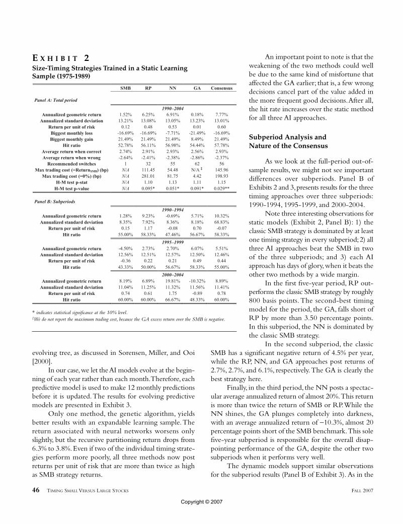
As we look at the full-period out-of-sample results, we might not see importantdifferences over subperiods. Panel B ofExhibits 2 and 3,presents results for the threetiming approaches over three subperiods:1990-1994, 1995-1999, and 2000-2004.

Note three interesting observations forstatic models (Exhibit 2, Panel B): 1) theclassic SMB strategy is dominated by at leastone timing strategy in every subperiod;2) allthree AI approaches beat the SMB in twoof the three subperiods; and 3) each AIapproach has days of glory,when it beats theother two methods by a wide margin.

In the first five-year period, RP out-performs the classic SMB strategy by roughly800 basis points. The second-best timingmodel for the period, the GA, falls short ofRP by more than 3.50 percentage points.In this subperiod, the NN is dominated bythe classic SMB strategy.

In the second subperiod, the classicSMB has a significant negative return of 4.5% per year,while the RP, NN, and GA approaches post returns of2.7%, 2.7%, and 6.1%, respectively.The GA is clearly thebest strategy here.

Finally, in the third period, the NN posts a spectac-ular average annualized return of almost 20%.This returnis more than twice the return of SMB or RP.While theNN shines, the GA plunges completely into darkness,with an average annualized return of −10.3%, almost 20percentage points short of the SMB benchmark.This solefive-year subperiod is responsible for the overall disap-pointing performance of the GA, despite the other twosubperiods when it performs very well.

The dynamic models support similar observationsfor the subperiod results (Panel B of Exhibit 3). As in the


E X H I B I T 2Size-Timing Strategies Trained in a Static Learning Sample (1975-1989)

* indicates statistical significance at the 10% level.‡We do not report the maximum trading cost, because the GA excess return over the SMB is negative.

Copyright © 2007

static case,note that each of the three approaches beats theother two in one of the three subperiods. In the case ofthe dynamic models, the SMB strategy cannot outperformany of the three AI approaches, except in the third sub-period, when it does better than RP and the GA.

The subperiod analysis clearly indicates that eachAI method tends to encounter periods of very good per-formance and periods of weaker performance, and thatsuccess and failure do not happen simultaneously for thethree methods. Such non-simultaneous periods of suc-cess and failure obviously translate into low correlations:−0.37 between the NN and the GA, −0.10 between RPand the GA,and 0.26 between RP and the NN. Not sur-prisingly, the three timing models yield the same deci-sions in only 49 of the 180 months (27.2%).

This non-simultaneity calls for aninvestigation into the power of consensus topredict which of large or small stocks willperform best in a given month.The idea isto tilt the capitalization favored by at leasttwo of the three AI approaches each month(a consensus strategy following a two-tiermajority rule).

The last columns in Exhibits 2 and 3present the performance of the consensusstrategy over the full period and the three sub-periods. Over the full period, the Exhibit 2static model consensus outperforms the SMBby more than 600 basis points annually. Inter-estingly, the consensus beats the SMB in everysubperiod, by margins of 9.0, 10.0, and 0.7percentage points in the first, second, and third subperiods,respectively.At the same time,the consensus is beaten by a single timingstrategy in each subperiod.Overall, the return,the hit rate, and the return per unit of risk ofthe consensus are higher than those of any of the individual approaches. For the dynamicconsensus in Exhibit 3,we see an increase inreturn overall of 83 basis points (8.60% annu-alized return versus 7.77%) and an impres-sive effect on the hit rate, which increasesfrom 57.8% to 64.4%.

Formal Test of Market Timing Ability

While some of the timing modelsmight have suffered from misfortune,others

may have simply been gifted by luck.To distinguish luckfrom real timing ability, we apply the non-parametricmarket-timing test of Henriksson and Merton [1981].7

The last two lines in Panel A in Exhibits 2 and 3report the p-stat and p-value (level of confidence) asso-ciated with this test. All the eight cases (AI approachesand consensus) have p-stat values significantly higher than1 at a level of confidence of at least 10%.The NN and theconsensus both reach the 1% level in their dynamic form.8

Practical Considerations

There are at least three practical issues to take intoaccount: outliers, transaction costs, and benchmarks andimplementation.


E X H I B I T 3Size-Timing Strategies Trained on an Expandable Learning Sample (1975 to Prediction)

**, *** indicate statistical significance at the 5% and 1% levels.

Copyright © 2007

Impact of outliers: We should note that the 2000-2004 subperiod is unique,marked by exceptionally goodperformance of the classic small-minus-big strategy.A closer examination of this subperiod quickly shows thatmost unusual return events (positive or negative) hap-pened in the year 2000. Indeed, we see in that year threemonthly returns higher than 10% in absolute value.Thisis highly abnormal, given that such extreme monthlyreturns have occurred only five times between 1926 and1999.We thus examine what happens with our timingmodels under such extreme conditions.

We are also interested in determining the behaviorof the models under more normal conditions, so wereevaluate the performance of the AI approaches and theconsensus and the SMB strategies in a normalized out-of-sample data set that excludes the year 2000. The resultsindicate all AI approaches have a return per unit of riskhigher than the return of the SMB strategy. Most notably,the return of the GA strategy increases from a disap-pointing average annualized return of 0.2% to a moreacceptable return of 2.9%.The average return of the con-sensus falls slightly, from 7.7% to 7.1%. For the dynamicmodels, the average increases from 8.6% to 9.3% when weexclude the year 2000.

Transaction cost considerations: One element inExhibits 2 and 3 that we have not yet explained is the number of required switches.To calculate this metric,we count one “required switch” every time the portfolioswitches from large-cap to small-cap, and vice versa.

If minimizing the number of switches and associatedtransaction costs is the primary objective, recursive parti-tioning (in its static form) is clearly the winner; it has only32 switches in 180 months, compared to 55 and 62 forthe NN and the GA (Panel A of Exhibit 2). In its dynamicform (Panel A of Exhibit 3), RP turns in the highestnumber of switches.The other two approaches requireabout the same number of switches in their static ordynamic forms.

Interestingly, the consensus requires 10 fewer switchesin the dynamic version (46 versus 56). It thus has twomain advantages: The majority rule produces strongerpredictive signals and hence better performance and fewer switches for the dynamic strategies, which are theones practitioners are most likely to follow.

We also calculate break-even transaction costs sothat a method yields either the same net return as theclassic SMB strategy or a null return.With the exceptionof the static GA, whose return is already lower than thereturn of the classic SMB strategy, all other five cases

remain relatively profitable compared to the classic SMB.The consensus strategy, in its dynamic form, can handletransaction costs of up to 165 basis points (i.e., break-eventransaction costs), while the RP strategy, in its dynamicform,can support transaction costs of up to 54 basis points.

We believe it is reasonable to assume that real trans-action costs are far lower than these values.

Benchmark and implementation: All results so faruse the SMB factor as the source of return.We decidedto use the longest possible history of data in training ourapproaches, even though the factor could be hard to repli-cate in practice. Some sensitivity analyses confirm thatour results are not sensitive to the size-premium bench-mark used—(S&P 600−S&P 500), (Russell 2,000−Rus-sell 1,000), or (Wilshire 1,750−Wilshire 750).

Some of these alternative benchmarks could be moremanageable for implementation purposes, thanks to theavailability of futures, swaps, or exchange-traded funds.For the Russell indexes in the dynamic case, the returnper unit of risk (hit rate) becomes 0.19 (55.0%) for theRP, 0.66 (62.2%) for NN, 0.49 (56.7%) for the GA, and0.9 (65.0%) for the consensus.This implementation pro-vides some comfort with respect to the results obtained.9

CONCLUSION

U.S. equity managers who might consider an alpha-generating strategy using a small-size bet would earn, onaverage, a positive expected alpha in the long run.Theycould also experience long periods of underperformance.The classic small-minus-big strategy, which systematicallyfavors small-caps, might well be too naive, and size timing,even if risky,can present an opportunity to add further value.

We show that strategies based on three artificial intel-ligence approaches—recursive partitioning, neural net-works,and genetic algorithms—could successfully time theU.S. size premium over the 1990-2004 period.Of the sixindividual timing strategies examined—three artificialintelligence approaches conditioned on historical data(1975-1989) and on recent data (1975-month precedingthe prediction)—five outperform the SMB premium.

None of the six timing strategies systematically out-performs the SMB strategy during the three five-year sub-periods examined. Yet a strategy based on the majorityrule (that is, a strategy favored by at least two of the threeartificial intelligence approaches) outperformed the SMBstrategy in each subperiod. Not only does the consensusstrategy benefit from stronger predictive signals,but it alsoallows the number of bets (transaction costs) to be reduced.


Copyright © 2007

COINt−1 + 0.4094 LEADt−0 + 0.3359 MOMt−1 + 0.1166EARNt−1 + 0.2360 DIVt−1 + 0.4717 GSCIt−1 + 0.1183 CAPt−1 −0.6987 INDt−1 − 0.4827 CSIt−1 + 1.8991 ISMt−1 + 0.0332 SAVt−1 + 0.1905 M2t−1 − 0.8035 CEXPt−1 + 1.7319 PPIt−1 +0.9418 NYSEt−1 + 0.6027 TRADt−1] > 0.0171, the model favorssmall-cap. Otherwise, the model favors large-cap.

7Like the hit rate, the non-parametric market-timing testof Henriksson-Merton [1981] focuses on the number of cor-rect predictions rather than on the level of the returns associ-ated with each decision.The output of this test, the p-statistic,requires first the calculation of the number of correctly pre-dicted positive months and the number of correctly predictednegative months.A significant p-stat (higher than 1) indicatesthat the model has genuine predictive ability.

wheren1: number of correctly predicted months SMB is pos-

itive;N1: number of months SMB is positive;n2: number of correctly predicted months SMB is

negative; andN2: number of months SMB is negative.

The p-value is calculated according to Park and Switzer[1996]:

where N = N1 + N2 and n = n1 + n2.8We also use the parametric market-timing test of

Henriksson-Merton [1981].The results are similar to results forthe non-parametric test (available on request).

9More detailed results for the static and dynamic casesusing Russell indexes are available from the authors.

REFERENCES

Ahmed, P., L.J. Lockwood, and S. Nanda.“Multistyle RotationStrategies.”The Journal of Portfolio Management, 28 (Spring 2002),pp. 17-29.

Amenc,N.,P.Malaise,L.Martellini, and D.Sfeir.“Tactical StyleAllocation—A New Form of Market Neutral Strategy.” Journalof Alternative Investments, Summer 2003, pp. 8-22.

p value

N

x

N

n xN

nn

N n

− =

−

∑1 2

3

1

1min( , )

p statnN

nN

− = +1

1

2

2


Five of the six timing strategies, as well as the consensusstrategies, remain profitable even after transaction costs.

Although all methods have their merits, recursivepartitioning could be favored for its much greater trans-parency and ease of interpretation. In the case of NN andGA, we deal mostly with black boxes. For investorsfavoring results over understanding, the black box syn-drome is not a serious issue,but when the model does fail(as each method does in one subperiod), the investor willfind it quite complex to see what went wrong, given theopaque nature of the model.

In this presentation,we consider only extreme bets,100% long in small-caps and 100% short in large-caps,and vice versa.This follows Fox [1999], who stresses thatmanagers with superior forecasting skills (60% hit rate orhigher) should favor more extreme tilts because theyimprove the entire range of possible returns. Still, we canreasonably conceive of less extreme strategies that wouldallow for neutral allocation when choices are less clear-cut.Therefore, considering three states of the world—small-cap tilt, large-cap tilt, and no tilt—could be moreinteresting, as it could yield stronger predictive signals andfewer switches (lower transaction costs).

ENDNOTES

The views expressed in this article are those of the authorsand do not necessarily reflect the position of the Caisse deDépôt et Placement du Québec.

1Suppose that after all observations are allocated downthe tree, 20 observations end up in a given node. If 9 of theseobservations are associated with binary case A, and 11 are asso-ciated with binary case B, then the level of purity at this nodeis 0.55. If a further split is possible so that 8 of the 9 A cases goto the right along with two of the B cases, the resulting rightand left descendant nodes will have purity levels of 0.8 and 0.9.Such an additional split would obviously be welcomed.

2The elite count refers to the number of individuals thatare directly cloned in the next generation.A cross-over fractionof 0.8 implies that 80% of the non-cloned individuals in the nextgeneration are obtained via reproduction rather than mutation.

3Liew and Vassalou [2000] go the other way and demon-strate that the return on the SMB portfolio conveys informa-tion on future GDP growth and that it could be useful inpredicting economic cycles.

4Coggin [1998] suggests timing models on macroeco-nomic factors to forecast style index returns.

5The full tree is available upon request.6The GA equation is: If [0.1977 TERMt−1 − 0.4317

CREDITt−1− 0.5819 TBILLt−1 − 1.2883 INFLt−1 + 0.7378

Copyright © 2007

Bauer, R.J., Jr. Genetic Algorithms and Investment Strategies.New York: John Wiley & Sons, 1994.

Black,F.“Estimating Expected Return.”Financial Analysts Journal,January/February 1995, pp. 168-171.

Breiman, L., J.H. Friedman, R.A. Olsen, and C.J. Stone. Classi-fication and Regression Trees. Belmont, CA:Wadsworth Interna-tional Group, 1984.

Campbell, J.Y., A.W. Lo, and A. C. MacKinlay. The Econometricsof Financial Markets.Princeton:Princeton University Press,1997.

Coggin,T.D.“Long-Term Memory in Equity Style Indexes.”The Journal of Portfolio Management,Winter 1998, pp. 37-46.

Cooper, M., H. Gulen, and M.Vassalou.“Investing in Size andBook-to-Market Portfolios Using Information about the Macro-economy: Some New Trading Rules.” Working paper,Graduate School of Business, Columbia University, 2001.

Fama, E., and K.R. French. “Common Risk Factors in theReturns on Stocks and Bonds.” Journal of Financial Economics, 33(1993), pp. 3-56.

————. “The Cross-Section of Expected Stock Returns.”Journal of Finance, 47 (1992), pp. 427-465.

————.“Multifactor Explanations of Asset Pricing Anom-alies.” Journal of Finance, 51 (1996), pp. 55-84.

Fox, S. “Assessing TAA Manager Performance.” The Journal ofPortfolio Management, 26 (Fall 1999), pp. 40-49.

Haykin, S. Neural Networks. New York: Macmillan, 1994.

Henriksson, R.D., and R.C. Merton. “On Market Timing and Investment Performance. II. Statistical Procedures for Eval-uating Forecast Skills.” Journal of Business,54 (1981),pp.513-517.

Jensen, G.R., R.R. Johnson, and J.M. Mercer.“The Inconsis-tency of Small-Firm and Value Stock Premiums.”The Journal ofPortfolio Management, 24 (Winter 1998), pp. 27-35.

Kao, D.L., and R.D. Shumaker.“Equity Style Timing.” Finan-cial Analysts Journal, January/February 1999, pp. 37-48.

Kester,G.W. “Market Timing with Small vs.Large Firm Stocks:Potential Gains and Required Predictive Ability.”Financial Ana-lysts Journal, September/October 1990, pp. 63-69.

Kingdon, J., and K.Feldman.“Genetic Algorithm and Applica-tions to Finance.” Applied Mathematical Finance, 2 (1995a),pp. 89-116.

————. “Neural Networks and Some Applications toFinance.” Applied Mathematical Finance, 2 (1995b), pp. 17-42.

Kryzanowski, L., M. Galler, and D.W.Wright.“Using ArtificialNeural Networks to Pick Stocks.” Financial Analysts Journal,July/August 1993, pp. 21-27.

Leinweber, D.“The Perils and Promise of Evolutionary Com-putation on Wall Street.”The Journal of Investing, 12 (Fall 2003),pp. 21-28.

Levis,M., and M.Liodakis.“The Profitability of Style RotationStrategies in the United Kingdom.” The Journal of Portfolio Management, 26 (Fall 1999), pp. 73-86.

Liew, J., and M.Vassalou. “Can Book-to-Market, Size andMomentum be Risk Factors that Predict Economic Growth?”Journal of Financial Economics, 57 (2000), pp. 221-245.

Medsker,L.,R.R.Trippi,and E.Turban.Neural Networks in Financeand Investing. Chicago: Probus Publishing Company, 1993.

Olden, J.D., M.K. Joy, and R.G.Death.“An Accurate Compar-ison of Methods for Quantifying Variable Importance in Artificial Neural Networks Using Simulated Data.” EcologicalModelling, 178 (2004), pp. 389-397.

Park,T.H., and L.N.Switzer.“Mean Reversion of Interest-RateTerm Premiums and Profits from Trading Strategies with Treasury Futures Spreads.” Journal of Futures Markets,16(3) (1996),pp. 331-352.

Reinganum,M.R.“The Significance of Market Capitalizationin Portfolio Management over Time.” The Journal of PortfolioManagement, 25 (Summer 1999), pp. 39-50.

Sorensen, E.H., K.L. Miller, and C.K. Ooi.“The Decision TreeApproach to Stock Selection.” The Journal of Portfolio Manage-ment, 27 (Fall 2000), pp. 42-52.

White, H.“A Reality Check for Data Snooping.” Econometrica,68 (September 2000), pp. 1097-1126.

To order reprints of this article, please contact Dewey Palmieri [email protected] or 212-224-3675.


Copyright © 2007

timing small versus large stocks -...

Documents