timothy taylor’s principles of microeconomics 3e€¦ · timothy taylor’s principles of...

Timothy Taylor’s

Principles of Microeconomics 3e Economics and the Economy

Timothy Taylor Managing Editor:

The Journal of Economic Perspectives Macalester College

+ Arguably the most clearly written book on the market + Used by over 200 instructors + 3e: all new design with high resolution graphs + 3e: thorough update of data, discussions, references, and examples + 3e: more attention to:

New tools of monetary policy in the US & the European Union Quantitative easing and "forward guidance," where monetary policy will be

roughly the same for the next few years

And the European Central Bank's role a lender of last resort

More on anti-trust legislation

Differentiators:

Taylor 3e is a mainstream book; it covers all the main topics in a balanced way

Taylor writes about the subject with no ideological axe to grind.

Book is remarkably well written with clear examples; comprehensive, but no fluff.

Focus on helping students solve problems – Taylor walks students through the problem-solving process.

Affordable Student Prices and Options!

For Instructors What's Changed For Students What's Changed

Instructor Manual New to 3e Loose-leaf Option New to 3e

Lecture Slides Overhauled for 3e Color Paperback Option New to 3e

Test Item File Expanded and Updated for 3e Lecture Guide New to 3e

Computerized Test Bank Expanded and Updated for 3e Sapling Web Assignments Updated for 3e

Sapling Web Assignments Updated for 3e Online Quizzes and eFlash Cards Will be updated in 2015

Instructor Resource Folder New to 3e Annual Reader from Tim's Blog Available for Spring Term 2015

Free use of Content/Graphs from Tim’s Blog New to 3e

To Review Online Textbook:

www.textbookmedia.com

To Request Paperback: [email protected]

PART I THE INTERCONNECTED ECONOMY

1 The Interconnected Economy 1

2 Choice in a World of Scarcity 12

3 International Trade 33

PART I I SUPPLY AND DEMAND

4 Demand and Supply 52

5 Labor and Financial Capital Markets 77

6 Globalization and Protectionism 91

PART III THE FUNDAMENTALS OF MICROECONOMIC THEORY

7 Elasticity 112

8 Household Decision Making 131

9 Cost and Industry Structure 150

10 Perfect Competition 166

11 Monopoly 186

12 Monopolistic Competition and Oligopoly 201

PART IV MICROECONOMIC POLICY ISSUES APPLICATIONS

13 Competition and Public Policy 216

14 Environmental Protection and Negative Externalities 231

15 Technology, Positive Externalities, and Public Goods 246

16 Poverty and Economic Inequality 260

17 Issues in Labor Markets: Unions, Discrimination, Immigration 279

18 Information, Risk, and Insurance 297

19 Financial Markets 311

20 Public Choice 331

APPENDIX CHAPTERS

1 Interpreting Graphs 340

8 Indifference Curves 352

19 Present Discounted Value 366

About the author: Tim Taylor’s career has been devoted to making complex economic ideas clear to students, policy makers and other professional econo-mists. Taylor is the founding and only managing editor of the Ameri-can Economic Association’s Journal of Economic Perspectives, which for more than 20 years has been an accessible source for state-of-the art economic thinking. Tim has won numerous teaching awards from his teaching stints at institutions like Stanford, the University of Min-nesota and Macalester College.

“Thank you very much for the opportunity to speak of why I am using the Taylor ‘s Textbooks, supported by Sapling's Home Work service. In a word, VALUE! Spoken three times...Value, Value, Value! Examples to illustrate definitions and concepts are representative of life experienced by limited resource students. They "get" the concepts in a context easily applied to their lives, without having to spend a for-tune! -- Harry Anderson, Luna College “I truly appreciate that the book is cost effective and comprehensive for my students. I can present a top-ic and they can get a strong foundation from Tim Taylor's text, then we can go into in-depth discussions as we relate the text material to the real world and other sources.” --- Shari Lyman, Community College of Southern Nevada

“Tim Taylor’s Principles is an excellent introductory text, with solid content comparable to that of far more expensive texts. Our students find it a most helpful learning aid and also deeply appreciate its rela-tively low cost.” -- William J. Murphy, New England Institute of Technology

“I got the book and, frankly, couldn't put it down. I have listened to all of Tim's' programs for The Teach-ing Company and find him to be an extremely knowledgeable economist, who has the ability to take com-plex issues and make them come alive. His book is really an extension of his rather amazing style.” - Bill Sciacca, Penn State-Scranton

“I'm a huge fan of Prof. Taylor and have listened to all of his recorded courses for The Teaching Company. Thanks for making me aware of Tim’s Blog. This is a great resource!” -- Peter Canellis, Vaughn College

“I found the Macro split to be clearly written, logically organized, and quite a good introduction to the basic macroeconomic canon. Frankly, for the price it can’t be beaten.” -- Michael Kuehlwein, Pomona College

“When I first came across Timothy Taylor's textbook I could hardly believe it - a nice text for a great price. I'm happy I switched. It is a godsend for students on a budget.” --Lester Hadsell, SUNY Oneonta

“Tim is also an award-winning teacher and a highly sought-after editor. The characteristics that have made him successful in these capacities are those I look for in an economic principles textbook — clear organization and sensible, engaging writing, with the content needed to challenge young, smart students. Because of TM’s quality-value package, I am extremely excited about assigning Tim’s textbook this fall.” --John Karl Scholz, UW-Madison “Taylor’s book has a unique approach that builds intuition in a rigorous way, with clear discussion and relevant examples. Other books promise that, but Taylor’s actually achieves it.” --Jeffrey Sundberg, Lake Forest College

Microeconomics

Economics and the Economy

Timothy Taylor Journal of Economic Perspectives

Macalester College

Third Edition

For instructors: • PowerPoint® slides • Computerized test disk

When ordering this title, use ISBN 1-930789-42-4To order the complete version, use ISBN 1-930789-26-2To order the Macro version, use ISBN 1-930789-88-2

Microeconomics: Economics and the Economy, Edition 3Copyright © 2014, 2011, 2008 Timothy Taylor. Published by Textbook Media.

ISBN-10: 1-930789-42-4ISBN-13: 978-1-930789-42-5

All rights reserved. No part of this publication may be reproduced or transmitted in any form or by any means, electronic or mechanical, including photocopying and recording, or by any information storage or retrieval system without the prior written permission of the author and the publisher.

Printed in the United States of America by Textbook Media

iii

Preface xviiAbout the Author xix


1 The Interconnected Economy 1 2 Choice in a World of Scarcity 12 3 International Trade 33

PART II SUPPLY AND DEMAND

4 Demand and Supply 52 5 Labor and Financial Capital Markets 77 6 Globalization and Protectionism 91


7 Elasticity 112 8 Household Decision Making 131 9 Cost and Industry Structure 150 10 Perfect Competition 166 11 Monopoly 186 12 Monopolistic Competition and Oligopoly 201


13 Competition and Public Policy 216 14 Environmental Protection and Negative Externalities 231 15 Technology, Positive Externalities, and Public Goods 246 16 Poverty and Economic Inequality 260 17 Issues in Labor Markets: Unions, Discrimination, Immigration 279

Brief Contents

iv Brief Contents

18 Information, Risk, and Insurance 297 19 Financial Markets 311 20 Public Choice 331

APPENDIX CHAPTERS

1 Interpreting Graphs 340 8 Indifference Curves 352 19 Present Discounted Value 366

Glossary G-1Index I-1

v

Preface xviiAbout the Author xix


1 The Interconnected Economy 1

What Is an Economy? 2Market-Oriented vs. Command Economies 2The Interconnectedness of an Economy 2

The Division of Labor 3Why the Division of Labor Increases Production 4Trade and Markets 4The Rise of Globalization 5

Microeconomics and Macroeconomics 6Microeconomics: The Circular Flow Diagram 7Macroeconomics: Goals, Frameworks, and Tools 9

Studying Economics Doesn’t Mean Worshiping the Economy 9Key Concepts and Summary 10Review Questions 11

2 Choice in a World of Scarcity 12

Choosing What to Consume 13A Consumption Choice Budget Constraint 13How Changes in Income and Prices Affect the Budget Constraint 13Personal Preferences Determine Specific Choices 15From a Model with Two Goods to the Real World of Many Goods 16

Choosing Between Labor and Leisure 16An Example of a Labor-Leisure Budget Constraint 16How a Change in Wages Affects the Labor-Leisure Budget Constraint 17Making a Choice Along the Labor-Leisure Budget Constraint 17

Choosing Between Present and Future Consumption 18Interest Rates: The Price of Intertemporal Choice 19The Power of Compound Interest 20An Example of Intertemporal Choice 21

Contents

vi Contents

Three Implications of Budget Constraints: Opportunity Cost, Marginal Decision-Making, and Sunk Costs 22

Opportunity Cost 22Marginal Decision-Making and Diminishing Marginal Utility 23Sunk Costs 24

The Production Possibilities Frontier and Social Choices 24The Shape of the Production Possibilities Frontier and Diminishing Marginal Returns 25Productive Efficiency and Allocative Efficiency 27Why Society Must Choose 28

Confronting Objections to the Economic Approach 28A First Objection: People, Firms, and Society Don’t Act Like This 29A Second Objection: People, Firms, and Society Shouldn’t Do This 29

Facing Scarcity and Making Trade-offs 31Key Concepts and Summary 31Review Questions 32

3 International Trade 33

Absolute Advantage 35A Numerical Example of Absolute Advantage and Trade 35Trade and Opportunity Cost 38Limitations of the Numerical Example 39

Comparative Advantage 39Identifying Comparative Advantage 40Mutually Beneficial Trade with Comparative Advantage 42How Opportunity Cost Sets the Boundaries of Trade 44Comparative Advantage Goes Camping 45The Power of the Comparative Advantage Example 45

Intra-industry Trade between Similar Economies 45The Prevalence of Intra-industry Trade between Similar Economies 45Gains from Specialization and Learning 46Economies of Scale, Competition, Variety 47Dynamic Comparative Advantage 48

The Size of Benefits from International Trade 49From Interpersonal to International Trade 50Key Concepts and Summary 51Review Questions 51

PART II SUPPLY AND DEMAND

4 Demand and Supply 52

Demand, Supply, and Equilibrium in Markets for Goods and Services 53Demand for Goods and Services 53

Contents vii

Supply of Goods and Services 53Equilibrium—Where Demand and Supply Cross 55

Shifts in Demand and Supply for Goods and Services 57The Ceteris Paribus Assumption 57An Example of a Shifting Demand Curve 57Factors That Shift Demand Curves 58Summing Up Factors That Change Demand 59An Example of a Shift in a Supply Curve 60Factors That Shift Supply Curves 61Summing Up Factors That Change Supply 62

Shifts in Equilibrium Price and Quantity: The Four-Step Process 62Good Weather for Salmon Fishing 63Seal Hunting and New Drugs 64The Interconnections and Speed of Adjustment in Real Markets 65

Price Ceilings and Price Floors in Markets for Goods and Services 65Price Ceilings 65Price Floors 68Responses to Price Controls: Many Margins for Action 69Policy Alternatives to Price Ceilings and Price Floors 71

Supply, Demand, and Efficiency 72Consumer Surplus, Producer Surplus, Social Surplus 72Inefficiency of Price Floors and Price Ceilings 73

Demand and Supply as a Social Adjustment Mechanism 75Key Concepts and Summary 75Review Questions 76

5 Labor and Financial Capital Markets 77

Demand and Supply at Work in Labor Markets 77Equilibrium in the Labor Market 78Shifts in Labor Demand 79Shifts in Labor Supply 80Technology and Wage Inequality: The Four-Step Process 80Price Floors in the Labor Market: Living Wages and Minimum Wages 81The Minimum Wage as an Example of a Price Floor 82

Demand and Supply in Financial Capital Markets 83Who Demands and Who Supplies in Financial Capital Markets 84Equilibrium in Financial Capital Markets 85Shifts in Demand and Supply in Financial Capital Markets 85The United States as a Global Borrower: The Four-Step Process 86Price Ceilings in Financial Capital Markets: Usury Laws 87

Don’t Kill the Price Messengers 88Key Concepts and Summary 90Review Questions 90

viii Contents

6 Globalization and Protectionism 91

Protectionism: An Indirect Subsidy from Consumers to Producers 92Demand and Supply Analysis of Protectionism 92Who Benefits and Who Pays? 94

International Trade and Its Effects on Jobs, Wages, and Working Conditions 95

Fewer Jobs? 95Trade and Wages 97Labor Standards 98

The Infant Industry Argument 99The Dumping Argument 100

The Growth of Anti-Dumping Cases 100Why Might Dumping Occur? 101Should Anti-Dumping Cases Be Limited? 101

The Environmental Protection Argument 101The Race to the Bottom Scenario 102Pressuring Low-Income Countries for Higher Environmental Standards 103

The Unsafe Consumer Products Argument 103The National Interest Argument 104How Trade Policy Is Enacted: Global, Regional, and National 106

The World Trade Organization 106Regional Trading Agreements 107Trade Policy at the National Level 108Long-Term Trends in Barriers to Trade 108

The Trade-offs of Trade Policy 109Key Concepts and Summary 110Review Questions 111


7 Elasticity 112

Price Elasticity of Demand 113Calculating the Elasticity of Demand 114A Possible Confusion, a Clarification, and a Warning 115

Price Elasticity of Supply 116Calculating the Elasticity of Supply 117

Elastic, Inelastic, and Unitary Elasticity 118Applications of Elasticity 120

Does Raising Price Bring in More Revenue? 120Passing on Costs to Consumers? 122Long-Run vs. Short-Run Impact 125

Contents ix

Elasticity as a General Concept 126Income Elasticity of Demand 127Cross-Price Elasticity of Demand 127Elasticity in Labor and Financial Capital Markets 127Stretching the Concept of Elasticity 128

Conclusion 129Key Concepts and Summary 129Review Questions 130

8 Household Decision Making 131

Consumption Choices 131Total Utility and Diminishing Marginal Utility 132Choosing with Marginal Utility 134A Rule for Maximizing Utility 135Measuring Utility with Numbers 135

How Changes in Income and Prices Affect Consumption Choices 135How Changes in Income Affect Consumer Choices 136How Price Changes Affect Consumer Choices 137The Logical Foundations of Demand Curves 138Applications in Business and Government 139

Labor-Leisure Choices 141The Labor-Leisure Budget Constraint 142Applications of Utility Maximizing with the Labor-Leisure Budget Constraint 143

Intertemporal Choices in Financial Capital Markets 144Using Marginal Utility to Make Intertemporal Choices 145Applications of the Model of Intertemporal Choice 147

The Unifying Power of the Utility-Maximizing Budget Set Framework 148Key Concepts and Summary 148Review Questions 149

9 Cost and Industry Structure 150

The Structure of Costs in the Short Run 152Fixed and Variable Costs 152Average Costs, Average Variable Costs, Marginal Costs 153Lessons Taught by Alternative Measures of Costs 155A Variety of Cost Patterns 156

The Structure of Costs in the Long Run 156Choice of Production Technology 157Economies of Scale 158Shapes of Long-Run Average Cost Curves 159The Size and Number of Firms in an Industry 161Shifting Patterns of Long-Run Average Cost 163

x Contents


10 Perfect Competition 166

Quantity Produced by a Perfectly Competitive Firm 167Comparing Total Revenue and Total Cost 167Comparing Marginal Revenue and Marginal Costs 169Marginal Cost and the Supply Curve 170Profits and Losses with the Average Cost Curve 170The Shutdown Point 172Short-Run Outcomes for Perfectly Competitive Firms 174

Entry and Exit in the Long-Run Output 175How Entry and Exit Lead to Zero Profits 175Economic Profit vs. Accounting Profit 176The Economic Function of Profits 177

Factors of Production in Perfectly Competitive Markets 177The Derived Demand for Labor 177The Marginal Revenue Product of Labor 178Are Workers Paid as Much as They Deserve? 180Physical Capital Investment and the Hurdle Rate 180Physical Capital Investment and Long-Run Average Cost 182

Efficiency in Perfectly Competitive Markets 182Conclusion 183Key Concepts and Summary 183Review Questions 184

11 Monopoly 186

Barriers to Entry 187Legal Restrictions 187Control of a Physical Resource 187Technological Superiority 188Natural Monopoly 188Intimidating Potential Competition 190Summing Up Barriers to Entry 190

How a Profit-Maximizing Monopoly Chooses Output and Price 191Demand Curves Perceived by a Perfectly Competitive Firm and by a Monopoly 191Total and Marginal Revenue for a Monopolist 191Marginal Revenue and Marginal Cost for a Monopolist 194Illustrating Monopoly Profits 195The Inefficiency of Monopoly 197

Contents xi


12 Monopolistic Competition and Oligopoly 201

Monopolistic Competition 202Differentiated Products 202Perceived Demand for a Monopolistic Competitor 202How a Monopolistic Competitor Chooses Price and Quantity 203Monopolistic Competitors and Entry 205Monopolistic Competition and Efficiency 207The Benefits of Variety and Product Differentiation 208

Oligopoly 208Why Do Oligopolies Exist? 209Collusion or Competition? 209The Prisoner’s Dilemma 209The Oligopoly Version of the Prisoner’s Dilemma 210How to Enforce Cooperation 212



13 Competition and Public Policy 216

Corporate Mergers 217Regulations for Approving Mergers 217The Four-Firm Concentration Ratio 218The Herfindahl-Hirschman Index 219New Directions for Antitrust 220

Regulating Anticompetitive Behavior 221When Breaking Up Is Hard to Do: Regulating Natural Monopolies 223

The Choices in Regulating a Natural Monopoly 223Cost-Plus versus Price Cap Regulation 225

The Great Deregulation Experiment 225Doubts about Regulation of Prices and Quantities 225The Effects of Deregulation 226Frontiers of Deregulation 227

Around the World: From Nationalization to Privatization 228Key Concepts and Summary 229Review Questions 229

xii Contents

14 Environmental Protection and Negative Externalities 231

Externalities 233Pollution as a Negative Externality 233Command-and-Control Regulation 234Market-Oriented Environmental Tools 235

Market-Friendly Environmental Tool #1: Pollution Charges 235Market-Friendly Environmental Tool #2: Marketable Permits 236Market-Friendly Environmental Tool #3: Better-Defined Property Rights 238Applying Market-Oriented Environmental Tools 239

The Benefits and Costs of U.S. Environmental Laws 239Benefits and Costs of Clean Air and Clean Water 240Marginal Benefits and Marginal Costs 241The Unrealistic Goal of Zero Pollution 242

International Environmental Issues 242The Trade-off between Economic Output and Environmental Protection 243Key Concepts and Summary 244Review Questions 245

15 Technology, Positive Externalities, and Public Goods 246

The Incentives for Developing New Technology 248Some Grumpy Inventors 248The Positive Externalities of New Technology 249Contrasting Positive Externalities and Negative Externalities 250

How to Raise the Rate of Return for Innovators 251Intellectual Property Rights 251Government Spending on Research and Development 253Tax Breaks for Research and Development 254Cooperative Research and Development 254A Balancing Act 254

Public Goods 255The Definition of a Public Good 255The Free Rider Problem 256The Role of Government in Paying for Public Goods 258

Positive Externalities and Public Goods 258Key Concepts and Summary 259Review Questions 259

Contents xiii

16 Poverty and Economic Inequality 260

Drawing the Poverty Line 261The Poverty Trap 263The Safety Net 265

Temporary Assistance for Needy Families 266Earned Income Credit (EIC) 266Food Stamps 267Medicaid 267Other Safety Net Programs 268

Measuring Income Inequality 268Income Distribution by Quintiles 268Lorenz Curve 269

Causes of Growing Income Inequality 271The Changing Composition of American Households 271A Shift in the Distribution of Wages 271

Government Policies to Reduce Income Inequality 273Redistribution 274The Ladder of Opportunity 274Inheritance Taxes 275

The Trade-off between Incentives and Income Equality 276Key Concepts and Summary 277Review Questions 278

17 Issues in Labor Markets: Unions, Discrimination, Immigration 279

Labor Unions 280Facts about Union Membership and Pay 281Higher Wages for Union Workers 282The Decline in U.S. Union Membership 284Concluding Thoughts about the Economics of Unions 287

Employment Discrimination 287Earnings Gaps by Race and Gender 287Investigating the Female/Male Earnings Gap 289Investigating the Black/White Earnings Gap 289Competitive Markets and Discrimination 291Public Policies to Reduce Discrimination 291An Increasingly Diverse Workforce 292

Immigration 292Historical Patterns of Immigration 293Economic Effects of Immigration 293Proposals for Immigration Reform 294


xiv Contents

18 Information, Risk, and Insurance 297

The Problem of Imperfect Information 298“Lemons” and Other Examples of Imperfect Information 298How Imperfect Information Can Affect Equilibrium Price and Quantity 299When Price Mixes with Imperfect Information about Quality 299Mechanisms to Reduce the Risk of Imperfect Information 300

Insurance and Imperfect Information 302How Insurance Works 302Risk Groups and Actuarial Fairness 304The Moral Hazard Problem 304The Adverse Selection Problem 306Government Regulation of Insurance 306


19 Financial Markets 311

How Businesses Raise Financial Capital 312Early-Stage Financial Capital 312Profits as a Source of Financial Capital 313Borrowing: Banks and Bonds 313Corporate Stock and Public Firms 314How Firms Choose between Sources of Financial Capital 315

How Households Supply Financial Capital 317Bank Accounts 317Bonds 319Stocks 320Mutual Funds 324Housing and Other Tangible Assets 324The Trade-offs between Return and Risk 325

How to Become Rich 327Why It’s Hard to Get Rich Quick: The Random Walk Theory 327Getting Rich the Slow, Boring Way 328

How Capital Markets Transform Financial Flows 328Key Concepts and Summary 329Review Questions 330

Contents xv

20 Public Choice 331

When Voters Don’t Participate 332Special-Interest Politics 333Identifiable Winners, Anonymous Losers 334Pork Barrels and Logrolling 334Voting Cycles 336Where Is Government’s Self-Correcting Mechanism? 336A Balanced View of Markets and Government 337Key Concepts and Summary 338Review Questions 339

APPENDIX CHAPTERS

1 Interpreting Graphs 340

Pie Graphs 341Bar Graphs 342Line Graphs 342

Line Graphs with Two Variables 342Time Series 345Slope 345Slope of Straight Lines in Algebraic Terms 346

Comparing Line Graphs with Pie Charts and Bar Graphs 347How Graphs Can Mislead 347

8 Indifference Curves 352

What Is an Indifference Curve? 352The Shape of an Indifference Curve 352The Field of Indifference Curves 354The Individuality of Indifference Curves 354

Utility-Maximizing with Indifference Curves 354Maximizing Utility at the Highest Indifference Curve 355

Changes in Income 356Responses to Price Changes: Substitution and Income Effects 357Indifference Curves with Labor-Leisure and Intertemporal Choices 359

A Labor-Leisure Example 359An Intertemporal Choice Example 361

Conclusion 364

xvi Contents

19 Present Discounted Value 366

Applying Present Discounted Value to a Stock 366Applying Present Discounted Value to a Bond 367Other Applications 368

Glossary G-1Index I-1

xvii

When authors describe their reasons for writing an eco-nomics textbook, it seems customary to proclaim lofty goals, like teaching students “to think like economists” so that they can become more informed voters and citi-zens. Paul Samuelson, the author of the most famous in-troductory economics textbook for the second half of the twentieth century, famously said: “I don’t care who writes a nation’s laws—or crafts its advanced treaties—if I can write its economics textbooks.” On my best days, I have sufficient time and energy to lift my eyes to the horizon, strike a statuesque pose, and proclaim exalted goals. But most of the time, I’m just a workaday teacher and my goals are more limited and concrete.

The pedagogical approach of this textbook is rooted in helping students master the tools that they need to solve problems for a course in introductory economics. Indeed, one of the great pleasures of writing the book is having the opportunity to share my teaching toolkit of step-by-step explanations, practical examples, and metaphors that stick in the mind. On quizzes and exams, I do not ask broad or open-ended questions about informed citizen-ship and thinking like an economist. At the most basic level, my goal for an economics class is that students should feel well-prepared for quizzes and exams.

The preparation that students need to perform well in an introductory economics class can be divided into three parts. First, an introductory economics class involves mastering a specialized vocabulary. I sometimes tell stu-dents that learning economics is akin to learning a foreign language—with the added difficulty that terms in eco-nomics like “demand” or “supply” or “money” sound like standard English, and thus learning economics often re-quires that students drop their preconceptions about what certain words mean.

Second, students need to acquire some basic analytical tools. There are four central analytical models in an intro-ductory economics course: budget constraints, supply and demand, cost curves, and aggregate demand–aggregate supply. These four models are used for a very wide vari-ety of applications; still, there are only four of them. There are also a few key formulas and equations to learn with regard to topics like growth rates over time and elasticity.

Third, students must learn to recognize when these terms and tools apply and to practice using them. I often tell students not to bother memorizing particular ques-tions and answers from the textbook or homework, be-cause my quiz and exam questions will ask them to apply what they have learned in contexts they have not seen be-fore. To provide a variety of contexts, this book describes many economic issues and events, drawn from recent times and past history, and also drawn both from U.S. and international experiences. When students see a concept or analytical skill applied in a number of ways, they learn to focus on the underlying and unifying idea. I’ve also found that students do take away knowledge of many economic events and episodes—although different students seem to focus on an unpredictable (to me) array of examples, which is perhaps as it should be in an introductory course.

As a workaday teacher, the goal of helping students master the material so that they can perform well on my quizzes and exams is lofty enough—and tough enough— for me. There’s an old joke that economics is the science of taking what is obvious about human behavior and mak-ing it incomprehensible. Actually, in my experience, the process works in the other direction. Many students spend the opening weeks of an introductory economics course feeling as if the material is difficult, even impossible, but by the middle and the end of the class, what seemed so difficult early in the term has become obvious and straightforward. As a course in introductory economics focuses on one lesson after another and one chapter after another, it’s easy to get tunnel vision. But when you raise your eyes at the end of class, it can be quite astonishing to look back and see how far you have come. As students apply the terms and models they have learned to a se-ries of real and hypothetical examples, they often find to their surprise that they have also imbibed a considerable amount about economic thinking and the real-world econ-omy. Learning always has an aspect of the miraculous.

As always, my family makes a significant contribution to the existence of this book. In the six years since the first edition, the U.S. and world economy has been convulsed by a Great Recession and then by an ungainly process of sluggish and partial recovery. The task of updating figures

Preface

xviii Preface

and examples for this third edition is inevitably large, but thinking about how to build connections from the con-cepts in the text to the economic events of the last few years made it larger. During the process of preparing this revised edition, my wife has dealt lovingly with a distract-ed husband; my children, with a father who was sleep- deprived or “at the office.” In a very real sense, then, this

book is from my dear ones to the students and instructors who use it. I hope that it serves you well.

Timothy Taylor St. Paul, Minnesota October 1, 2013

xix

Timothy T. Taylor Timothy T. Taylor has been the Managing Editor of the Journal of Economic Perspectives, published by the American Economic Association, since the first issue of the journal in 1987. All issues of the journal are freely available online at http://e-jep.org. Taylor holds a B.A de-gree in economics and political science from Haverford College. He holds an M.S. degree in economics from Stanford University, where he focused on public finance, industrial organization, and economic history.

Taylor has taught economics in a variety of contexts. In 2012, his book The Instant Economist: Everything You Need to Know About How the Economy Works, was pub-lished by Penguin Plume. It was named an “Outstanding Academic Title” by Choice magazine of the American Li-brary Assocation and was also listed as one of the Best Books for 2012 in the “Business” category by Library Journal. He has recorded a variety of lecture courses for The Teaching Company, based in Chantilly, Virginia, in-cluding Economics (3rd edition), Unexpected Economics, America and the New Global Economy, Legacies of Great Economists, and History of the U.S. Economy in the 20th Century. In 1992, he won the Outstanding Teacher Award from the Associated Students of Stanford University. In 1996, he was named a Distinguished Instructor for his courses in introductory economics at the University of Minnesota. In 1997, he was voted Teacher of the Year by students at the Humphrey Institute of Public Affairs at the University of Minnesota.

He has published articles on various topics in eco-nomics in publications such as the Milken Institute Re-view, the Cato Journal, Public Interest, and the Journal of Economic Perspectives. He blogs regularly at http:// conversableeconomist.blogspot.com.

About the Author

112

A demand curve shows that a higher price will lead to a lower quantity demanded. But how much lower? A supply curve shows that a higher price will lead to a higher quantity supplied. But how much higher?

Whether a change in price will affect quantity demanded or quantity supplied by a relatively large or small amount often has real practical significance. For example, the average tax per pack on cigarettes was $2.35 in 2011, including both federal and state-level taxes. Taxes on cigarettes serve two purposes: to raise tax revenue for government and to discourage consumption of cigarettes. But if a higher cigarette tax discourages cigarette consumption by quite a lot, then because a greatly reduced quantity of cigarettes is sold, the cigarette tax on each pack won’t raise much revenue for the government. Alternatively, a higher cigarette tax that doesn’t discourage cigarette consumption by much will actually raise more tax revenue for the government. Thus, when a govern-ment agency tries to calculate the effects of altering its cigarette tax, it must analyze how much the tax affects the quantity of cigarettes consumed.

This issue reaches beyond governments and taxes; every firm faces a sim-ilar issue. Every time a firm considers raising the price that it charges, it must consider how much a price increase will reduce the quantity demanded of what it sells. Conversely, when a firm reduces its sales price, it must expect (or hope) that the lower price will lead to a higher quantity demanded of its product.

This chapter introduces the concept of elasticity, which measures how much a percentage change in price leads to a percentage change in quantity demanded or quantity supplied. The chapter begins with the price elasticity of demand, which looks at the responsiveness of quantity demanded to a change

elasticity: How much a percentage change in quantity demanded or quantity supplied is affected by a percentage change in price.

CHAPTER Elasticity 7

Chapter 7 Elasticity 113

in price, and then examines the price elasticity of supply, which looks at the responsive-ness of quantity supplied to a change in price. The concept of elasticity is then applied to a number of real-world situations, including ticket prices at concerts, cigarette taxes, airline ticket prices, changes in world oil prices, and others.

Price Elasticity of DemandWhen investigating how sensitive the quantity demanded is to a change in price, looking at the demand curve might seem like an obvious starting point. But the visual appear-ance of demand curves can be misleading. Exhibit 7-1 illustrates the problem. The data on price and quantity demanded of cheese for Exhibit 7-1a and 7-1b is identical. But in Exhibit 7-1a, the demand curve for cheese is graphed with a tall vertical axis and narrow horizontal axis, so that the demand curve appears to slope down steeply. In Exhibit 7-1b, the identical data is graphed with a short vertical axis and a wide horizontal axis, so that the demand curve appears to slope down in a relatively flat way. Remember, the data behind these two demand curves is exactly the same! In both Exhibit 7-1a and 7-1b, the demand curve slopes down, but should the shape of the demand curve for cheese be de-scribed as “steep” or “flat”? Answering this question with “it depends on how you draw it” is not very useful.

The vocabulary of elasticity offers a method of discussing how quantity demanded responds to changes in price that doesn’t depend on whether the axes are drawn rela-tively longer or shorter. It doesn’t even depend on what units are used to measure price and quantity. Instead of trying to discuss the steepness or flatness of supply and demand curves based on their visual appearance, which can be misleading, elasticity discusses the shape of demand and supply curves with numerical calculations of percentage changes.

Price per Pound Quantity Demanded in Pounds$2.00 900,000$2.50 700,000$3.00 600,000$3.50 550,000$4.00 500,000

EXHIBIT 7-1 Same Data for Demand Curve, Different Appearance These two demand curves present exactly the same data on price and quantity. The only difference is that (a) is drawn with a longer vertical axis, while (b) is drawn with a longer horizontal axis. Both demand curves still slope down, but whether the slope appears steep or flat is determined by how the curve is drawn, not by the data.

400 500 700 900 1,000$0.00

P

Demand

R

S

T

U

V

800600

(a)

$4.50

Q (thousands of pounds)

$4.00

$3.50

$2.50

$1.50

$0.50

$1.00

$2.00

$3.00

400 500 700 900 1,000$0.00

P

800600

(b)

$4.50

Q (thousands of pounds)

$4.00$3.50

$2.50

$1.50

$0.50$1.00

$2.00

VU

TS

R

Demand

$3.00

114 Chapter 7 Elasticity

Calculating the Elasticity of DemandThe numerical example of a demand curve D for small television sets presented in Ex-hibit 7-2 can help to illustrate the issues. In this case, this demand curve for small television sets is a straight line. Let’s calculate the elasticity between points A and B and between points G and H. The elasticity of demand is defined as the percentage change in quantity demanded divided by the percentage change in price. The percentage change between two quantities is calculated by taking the difference between the two quantities and dividing by the average of the two quantities—which will be the point halfway between the two quan-tities. Similarly, the percentage change between two prices is calculated by taking the dif-ference between the two prices and dividing by the average of the two prices—which will be the point halfway between the two prices. Thus, the formula for elasticity of demand is:

Elasticity of demand = % change in quantity demanded% change in price

= (difference in quantity / average of original quantities)(difference in price / average of original prices)

First, apply this formula to the elasticity between A to B:

= =[3,000 – 2,800] / [(3,000 + 2,800) / 2][60 – 70] / [(60 + 70) / 2]

200/2,900–10/65

0.069–0.154

Therefore, the elasticity of demand between these two points is = –0.069/0.154 = –0.448.As a second example, apply the same formula to calculating the elasticity of demand

from G to H.

=[1,600 – 1,800] / [(1,600 + 1,800) / 2][130 – 120] / [(130 + 120) / 2]

= –200/170010/125

–0.11760.08

Therefore, the elasticity of demand from G to H is = –0.1176/0.08 = –1.47.

elasticity of demand: The percentage change in quantity demanded divided by the percentage change in price.

Points P QA 60 3,000B 70 2,800C 80 2,600D 90 2,400E 100 2,200F 110 2,000G 120 1,800H 130 1,600

EXHIBIT 7-2 Calculating the Price Elasticity of Demand The price elasticity of demand is calculated as the percentage change in quantity divided by the percentage change in price. Between two points like A and B, or between G and H, the formula is:

Elasticity = (change in quantity)/[(sum of the two quantities/2)](change in price)/[(sum of prices/2)]

1,500 2,500 3,000$40

P

H

(1600,130)

(1800,120)

F (2000,110)

E (2200,100)

(2400,90)

(2600,80)

(2800,70)

(3000,60)

2,000

$150

Q

$120

$90

$60

G

D

C

B

A


An elasticity number is not followed by any units. Elasticity is a ratio of one percentage change to another percentage change—nothing more.

Calculations of elasticity are all arithmetic, so what is the intuitive meaning of the number that emerges from the calculation? Hark back to the original meaning of elas-ticity: that is, the change in quantity demanded that results from a percentage change in price. Thus, if the price started off at 65—midway between the price at points A and B in the example—then a 10% increase in price of small televisions would cause a 4.48% reduction in quantity demanded, or conversely, a 10% fall in price would cause a 4.48% increase in the quantity demanded of small televisions. However, if the price started off in the range between 120 and 130—that is, midway between prices at points G and H in the example—then a 10% percent increase in price would cause a 14.7% decline in quantity demanded of small televisions, or conversely, a 10% fall in price would cause a 14.7% rise in the quantity demanded.

The word “elasticity,” in its everyday use, refers to stretchiness: more elastic stretches more, while less elastic stretches less. The elasticity of demand has the same general meaning, except that in this case the stretchiness refers to how much the quantity demand-ed stretches or contracts in response to a change in price. Exhibit 7-3 shows a selection of demand elasticities for different goods and services drawn from a variety of different studies by economists. A typical practice in these studies is to calculate the elasticity of demand using the current market equilibrium as the starting point.

A Possible Confusion, a Clarification, and a WarningThe most common confusion about elasticity is to think that it measures the slope of the demand curve. Elasticity is not the slope of the demand curve! The examples above have shown that whether a demand curve appears to have a steep or a flat slope depends on how it is drawn. Even when the demand curve is a straight line, with the same mathemat-ical slope at all points, the elasticity will differ quite substantially in different parts of that line. The calculation of elasticity is based on percentage change, which is not the same as the calculation for slope.

Many students who are confronted with the elasticity formula wonder why, in the numerator and denominator, the formula divides by the average value of either the two quantities (in the numerator) or the two prices (in the denominator). The reason is to avoid a situation where in calculating the elasticity between points A and B, one person divides the change in quantity by the quantity level at A while another divides it by the quantity level at B—thus leading to two different answers for the same question. By using the

EXHIBIT 7-3 Some Selected Elasticities of Demand

Coal 0.11 Radio and TV 0.71

Cameras 0.15 Beef 0.75

Housing 0.18 Soft drinks 0.79

Wine 0.24 New automobiles 0.87

Coffee 0.3 Railway 1.08

Electricity 0.3 Air travel 1.15

Gasoline 0.31 2% milk 1.22

Kitchen and household appliances 0.4 Internet 1.29

Spirits 0.6 Restaurant meals 1.42

Poultry 0.68 Computer 2.17


average quantity and average price between A and B, this possible confusion is eliminat-ed. At a more advanced level of economics, using the tools of calculus, elasticity can be calculated at a specific point—in which case the need to divide by the average quantity and price at two different points doesn’t arise.

Finally, here’s a warning: Because demand curves slope down, the percentage change in quantity demanded in response to a percentage change in price will be a negative number— that is, either a higher price leads to a lower quantity demanded, or a lower price leads to a higher quantity demanded. However, economists have often dropped the negative sign on the elasticity of demand for decades now. After all, economists know that demand curves generally slope downward, so they don’t need the reminder of the negative sign. So when you are reading or listening to something about economics and run across an elasticity of demand that has no negative sign, don’t be surprised.

Price Elasticity of SupplyJust as the price elasticity of demand reveals how a percentage change in price will lead to a percentage change in quantity demanded, the price elasticity of supply measures how a percentage change in price will lead to a percentage change in quantity supplied. Again, the elasticity cannot be easily inferred from glancing at the appearance of a supply curve. Instead, elasticity requires a numerical calculation.

Elasticity Is Not Slope

CLEARING IT UP

Although the elasticity of a supply or demand curve is obviously related to the shape of the curve, it isn’t the same as what the mathematicians call “slope.” Not even close. Slope, you may remember from a high school mathematics class (or from the Appendix to Chapter 1), is “rise over run”; that is, the change on the vertical axis (the rise) divided by the change on the hor-izontal axis (the run). This calculation differs from elas-

ticity in two ways. First, elasticity involves the change in what is on the horizontal axis (quantity) divided by the change in what is on the vertical axis (price). Thus, elasticity involves run/rise, not rise/run. Second, elas-ticity is the percentage change, which is a different cal-culation from slope. A straight line has only one slope, but as the example in the chapter shows, a straight-line demand curve has a different elasticity at every point.

Elasticity in the Vending Machine

America has 1.5 million vending machines that sell snacks and candy. Tens of millions of Americans are overweight. Could vending machines be used to nudge people toward a healthier diet? A group of researchers in the School of Public Health at the University of Min-nesota have been carrying out studies to see how price and availability of snacks in vending machines affect people’s purchases.

For example, one of their studies focused on vend-ing machines at 12 worksites and 12 schools. They of-fered a range of price cuts for low-fat snacks. On some of the machines, they also posted signs identifying the low-fat snacks and encouraging people to buy them. The signs encouraging people to eat low-fat foods had little effect. But the study found that elasticity of de-mand for low-fat snacks is about 2. That is, a 10% cut in the price of low-fat snacks led to an increase of 20%

in the quantity of such snacks consumed, and a 50% cut in the price of such snacks led to an increase of 100% in sales of low-fat snacks. As it turned out, the price cuts for low-fat snacks didn’t even cause the av-erage profits per vending machine to decline because an increase in the volume sold was enough to compen-sate for the lower prices.

Another one of their studies looked at vending ma-chines in four metropolitan bus garages. In this study, they cut prices for healthy snack options by an aver-age of 30% and also made sure that healthier snacks represented half of the choices in these vending ma-chines. In this study, the elasticity of demand for health snacks was about 1: that is, the 30% fall in prices for healthy snacks led to a rise of about 30% in the quan-tity consumed of these snacks.


Calculating the Elasticity of SupplyAssume that you are renting an apartment in the Philadelphia metropolitan area, where the cost of housing for renters is about $650 per month. Say that your neighborhood has 10,000 rental units. This situation is illustrated in both Exhibit 7-4a and Exhibit 7-4b, where the original equilibrium in both graphs is at a price of $650 and a quantity of 10,000 rental apartments. Now imagine that your neighborhood suddenly becomes a more popu-lar and fashionable place to live—that is, demand for rental housing in your neighborhood shifts to the right. Both Exhibit 7-4a and Exhibit 7-4b show an identical shift of a demand curve for rental housing out to the right from D0 to D1. However, the shape of the supply curve for rental housing differs in the two graphs. As a result, in Exhibit 7-4a, the new equilibrium E1 in your neighborhood occurs at a higher rental price of $900 per month and a slightly higher equilibrium quantity of 11,000 rental units, while in Exhibit 7-4b, the new equilibrium E1 results in a slightly higher rental price of $700 per month and a substantially higher equilibrium quantity of 13,000 rental units in your neighborhood. The elasticity of supply is a useful tool for explaining the different outcomes in these two situations.

Let’s begin with the calculations. The elasticity of supply is defined as the percentage change in quantity supplied divided by the percentage change in price. Again, the per-centage change between two quantities is calculated by taking the difference between the two quantities and dividing by the average of the two quantities. Similarly, the percentage change between two prices is calculated by taking the difference between the two prices and dividing by the average of the two prices. Thus, the formula for elasticity of supply is:

Elasticity of supply = % change in quantity supplied% change in price

= (change in quantity / average of original quantities)(change in price / average of original prices)

elasticity of supply: The percentage change in quantity supplied divided by the percentage change in price.

EXHIBIT 7-4 How a Shift in Demand Can Affect Price or Quantity MoreThe intersection E0 between supply curve S and demand curve D0 is the same in both (a) and (b). The increase in demand from D0 to D1 is the same in both (a) and (b). The new equilibrium E1 has a higher price and quantity than the original equilibrium E0 in both (a) and (b). However, the shape of supply differs in (a) and (b). As a result, in (a), the new equilibrium E1 happens at a much higher price but only a small increase in quantity, while in (b), the new equilibrium happens at only a small increase in price but a relatively large increase in quantity.

5 10 15

$100

(a) Shifting Demand, Inelastic Supply

P (

$/m

on

th)

20

S

D0

D1

E1 (11,000, $900)

E0 (10,000, $650)

Q (1,000s of rental units)

$900

$800

$600

$400

$200

$300

$500

$700

5 10 15

$100

(b) Shifting Demand, Elastic Supply

P (

$/m

on

th)

20

S

D0

D1

E1 (13,000, $700)

Q (1,000s of rental units)

$900

$800

$600

$400

$200

$300

$500

$700

E0 (10,000, $650)


First, apply this formula to the elasticity of supply between E0 and E1 in Exhibit 7-4a.

[11,000 – 10,000] / [(11,000 + 10,000) / 2][900 – 650] / [(900 + 650) / 2]

= 1,000/10,500250/775

= .095.322

The elasticity of supply in this example is .095/.322 = .295.Now apply the same formula for elasticity of supply to the change between E0 and E1

in Exhibit 7-4b.

[13,000 – 10,000] / [(13,000 + 10,000) / 2][700 – 650] / [(700 + 650) / 2]

= 3,000/11,50050/675

= .261.074

The elasticity of supply in this case is .261/.074 = 3.52.Again, as with the elasticity of demand, the elasticity of supply is not followed by

any units. Elasticity is a ratio of one percentage change to another percentage change— nothing more.

What is the intuitive meaning of these calculations? The elasticity of supply in Ex-hibit 7-4a is relatively small. A 10% rise in price causes only a 2.9% rise in the quantity supplied in Exhibit 7-4a. The elasticity of supply in Exhibit 7-4b is relatively large. In this case, a 10% rise in price would bring an increase in supply of 35%. The much greater elasticity of supply in Exhibit 7-4b means that quantity supplied will react much more to a certain percentage change in price.

In situations like this one, the supply curve in Exhibit 7-4a often reflects the situation in the short-term, when the quantity supplied of rental housing cannot increase much in the short term of a year or two. As a result, the elasticity of supply is fairly low, and the increase in demand is primarily reflected in higher prices. However, the supply curve in Exhibit 7-4b makes more sense from the longer run perspective of several years, when the quantity supplied of housing has time to rise more substantially because of new building activity or converting existing properties into rental units. As a result, in the long run the very same rise in demand is reflected more in a rise in the quantity of housing and less in a rise in price.

Elastic, Inelastic, and Unitary ElasticityNumerical measures of elasticity can be usefully divided into three broad categories: elas-tic, inelastic, and unitary elasticity. The categories are summarized in Exhibit 7-5.

When quantity demanded or supplied is highly sensitive to changes in price, it is said to be elastic. Specifically, an elastic demand refers to a situation in which a certain percentage change in price leads to a larger percentage change in quantity demanded or quantity sup-plied. For example, a 1% rise in the price would cause a decline of more than 1%—perhaps 2%—in the quantity demanded of a good. Since elasticity refers to the percentage change in quantity divided by the percentage change in price, saying that a demand curve or supply curve is elastic means that the elasticity calculated from the formula is greater than 1.

elastic: The elasticity calculated from the appropriate formula has an absolute value greater than 1.

EXHIBIT 7-5 Elastic, Unitary, and Inelastic: Three Cases of Elasticity

If . . . Then . . . And It’s Called . . .

% change in quantity > % change in price >% change in quantity% change in price 1 Elastic

% change in quantity = % change in price =% change in quantity% change in price 1 Unitary elasticity

% change in quantity < % change in price <% change in quantity% change in price 1 Inelastic


Demand will be elastic when consumers find it easy to shift back and forth between goods and services. For example, if the price of lamb rises, many consumers will shift to other meats and foods. Supply will be elastic when it is relatively easy to expand or contract production. For example, at a time when most of the factories in an industry are running at only about half of their full production level, it will be relatively easy to ramp up production higher.

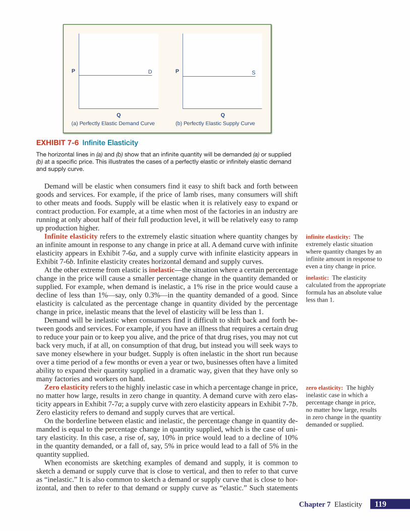
Infinite elasticity refers to the extremely elastic situation where quantity changes by an infinite amount in response to any change in price at all. A demand curve with infinite elasticity appears in Exhibit 7-6a, and a supply curve with infinite elasticity appears in Exhibit 7-6b. Infinite elasticity creates horizontal demand and supply curves.

At the other extreme from elastic is inelastic—the situation where a certain percentage change in the price will cause a smaller percentage change in the quantity demanded or supplied. For example, when demand is inelastic, a 1% rise in the price would cause a decline of less than 1%—say, only 0.3%—in the quantity demanded of a good. Since elasticity is calculated as the percentage change in quantity divided by the percentage change in price, inelastic means that the level of elasticity will be less than 1.

Demand will be inelastic when consumers find it difficult to shift back and forth be-tween goods and services. For example, if you have an illness that requires a certain drug to reduce your pain or to keep you alive, and the price of that drug rises, you may not cut back very much, if at all, on consumption of that drug, but instead you will seek ways to save money elsewhere in your budget. Supply is often inelastic in the short run because over a time period of a few months or even a year or two, businesses often have a limited ability to expand their quantity supplied in a dramatic way, given that they have only so many factories and workers on hand.

Zero elasticity refers to the highly inelastic case in which a percentage change in price, no matter how large, results in zero change in quantity. A demand curve with zero elas-ticity appears in Exhibit 7-7a; a supply curve with zero elasticity appears in Exhibit 7-7b. Zero elasticity refers to demand and supply curves that are vertical.

On the borderline between elastic and inelastic, the percentage change in quantity de-manded is equal to the percentage change in quantity supplied, which is the case of uni-tary elasticity. In this case, a rise of, say, 10% in price would lead to a decline of 10% in the quantity demanded, or a fall of, say, 5% in price would lead to a fall of 5% in the quantity supplied.

When economists are sketching examples of demand and supply, it is common to sketch a demand or supply curve that is close to vertical, and then to refer to that curve as “inelastic.” It is also common to sketch a demand or supply curve that is close to hor-izontal, and then to refer to that demand or supply curve as “elastic.” Such statements

infinite elasticity: The extremely elastic situation where quantity changes by an infinite amount in response to even a tiny change in price.

inelastic: The elasticity calculated from the appropriate formula has an absolute value less than 1.

zero elasticity: The highly inelastic case in which a percentage change in price, no matter how large, results in zero change in the quantity demanded or supplied.

EXHIBIT 7-6 Infinite Elasticity The horizontal lines in (a) and (b) show that an infinite quantity will be demanded (a) or supplied (b) at a specific price. This illustrates the cases of a perfectly elastic or infinitely elastic demand and supply curve.

(a) Perfectly Elastic Demand Curve

D

Q

P

(b) Perfectly Elastic Supply Curve

S

Q

P


must be handled with care. Remember, a close-to-horizontal or close-to-vertical demand or supply curve may appear that way because of how the axes are drawn, not because of some inherent characteristic of the underlying data. Moreover, elasticity will usually vary along a demand or supply curve, so that one zone of a demand or supply curve can be elastic while another zone is inelastic. Nonetheless, for purposes of sketching diagrams and illustrating economic intuition, it is often convenient to treat inelastic as close to ver-tical and elastic as close to horizontal. As long as one remembers that such statements are only approximations for the purposes of illustration, no harm is done.

Applications of ElasticityElasticities are useful in a wide range of circumstances. Even knowing only that a demand or supply curve is elastic or inelastic can lead to interesting insights.

Does Raising Price Bring in More Revenue?Imagine that a band on tour is playing in an indoor arena with 15,000 seats. To keep this example simple, assume that the band keeps all the money from ticket sales. (For ex-ample, you can imagine that the owners of the arena make their money by charging for parking and concessions.) Assume further that the band pays the costs for its appearance, but that these costs like travel, setting up the stage, and so on, are the same regardless of how many people gather in the audience. Finally, assume that all the tickets have the same price. (The same insights apply if ticket prices are more expensive for some seats than for others, but the calculations become more complicated.) The band knows that it faces a downward-sloping demand curve; that is, if the band raises the price of tickets, it will sell fewer tickets. How should the band set the price for tickets to bring in the most total revenue, which in this example, because costs are fixed, will also mean the highest profits for the band? Should the band sell more tickets at a higher price or fewer tickets at a lower price?

The key concept in thinking about collecting the most revenue is the elasticity of de-mand. Total revenue is price times the quantity of tickets sold. Imagine that the band starts off thinking about a certain price, which will result in the sale of a certain quantity of tickets. The three possibilities are laid out in Exhibit 7-8. If demand is elastic at that price level, then the band should cut the price because the percentage drop in price will result in an even larger percentage increase in the quantity sold—thus raising total revenue. However, if demand is inelastic at that original quantity level, then the band should raise

EXHIBIT 7-7 Zero Elasticity The (a) vertical demand and (b) vertical supply curves show that there will be zero percentage change in quantity demanded or supplied, regardless of the price. This illustrates the case of zero or perfect inelasticity.

(a) Perfectly Inelastic Demand Curve

D

Q

P

(b) Perfectly Inelastic Supply Curve

S

Q

P


What Does a Unitary Elasticity of Demand or Supply Look Like?

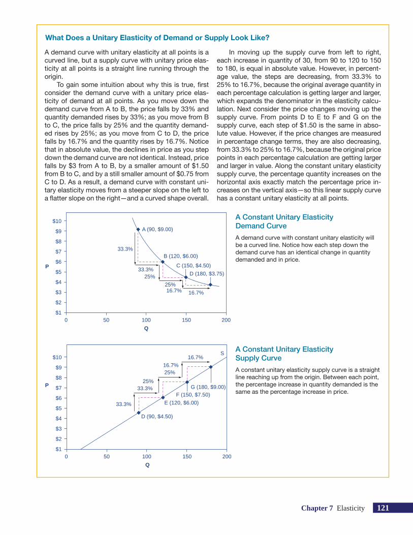
A demand curve with unitary elasticity at all points is a curved line, but a supply curve with unitary price elas-ticity at all points is a straight line running through the origin.

To gain some intuition about why this is true, first consider the demand curve with a unitary price elas-ticity of demand at all points. As you move down the demand curve from A to B, the price falls by 33% and quantity demanded rises by 33%; as you move from B to C, the price falls by 25% and the quantity demand-ed rises by 25%; as you move from C to D, the price falls by 16.7% and the quantity rises by 16.7%. Notice that in absolute value, the declines in price as you step down the demand curve are not identical. Instead, price falls by $3 from A to B, by a smaller amount of $1.50 from B to C, and by a still smaller amount of $0.75 from C to D. As a result, a demand curve with constant uni-tary elasticity moves from a steeper slope on the left to a flatter slope on the right—and a curved shape overall.

In moving up the supply curve from left to right, each increase in quantity of 30, from 90 to 120 to 150 to 180, is equal in absolute value. However, in percent-age value, the steps are decreasing, from 33.3% to 25% to 16.7%, because the original average quantity in each percentage calculation is getting larger and larger, which expands the denominator in the elasticity calcu-lation. Next consider the price changes moving up the supply curve. From points D to E to F and G on the supply curve, each step of $1.50 is the same in abso-lute value. However, if the price changes are measured in percentage change terms, they are also decreasing, from 33.3% to 25% to 16.7%, because the original price points in each percentage calculation are getting larger and larger in value. Along the constant unitary elasticity supply curve, the percentage quantity increases on the horizontal axis exactly match the percentage price in-creases on the vertical axis—so this linear supply curve has a constant unitary elasticity at all points.

0 50 100 150 200$1

P

A (90, $9.00)

B (120, $6.00)

C (150, $4.50)

D (180, $3.75)

33.3%

33.3%

25%16.7% 16.7%

25%

$10

Q

$9

$8

$6

$4

$2

$3

$5

$7

A Constant Unitary Elasticity Demand Curve A demand curve with constant unitary elasticity will be a curved line. Notice how each step down the demand curve has an identical change in quantity demanded and in price.

A Constant Unitary Elasticity Supply Curve A constant unitary elasticity supply curve is a straight line reaching up from the origin. Between each point, the percentage increase in quantity demanded is the same as the percentage increase in price.

0 50 100 150 200$1

P

S

D (90, $4.50)

E (120, $6.00)

F (150, $7.50)G (180, $9.00)

33.3%

33.3%

25%

25%

16.7%

16.7%$10

Q

$9

$8

$6

$4

$2

$3

$5

$7


the price of tickets because a certain percentage increase in price will result in a smaller percentage decrease in the quantity sold—and total revenue will rise. If demand has a unitary elasticity at that quantity, then a moderate percentage change in the price will be offset by an equal percentage change in quantity—so the band will earn the same revenue whether it (moderately) increases or decreases the price of tickets.

What if the band keeps cutting price, because demand is elastic, until it reaches a level where all 15,000 seats in the available arena are sold? If demand remains elastic at that quantity, the band might try to move to a bigger arena, so that it could cut ticket prices further and see a larger percentage increase in the quantity of tickets sold. Of course, if the 15,000-seat arena is all that is available or if a larger arena would add substantially to costs, then this option may not work.

Conversely, a few bands are so famous, or have such fanatical followings, that demand for tickets may be inelastic right up to the point where the arena is full. These bands can, if they wish, keep raising the price of tickets. Ironically, some bands that are extremely popular among a smaller group could make more revenue by setting prices so high that the arena is not filled—but those who buy the tickets would have to pay very high prices. However, bands sometimes choose to sell tickets for less than the absolute maximum they might be able to charge, often in the hope that fans will feel happier about attending the concert and spend more on recordings, T-shirts, and other paraphernalia.

Passing on Costs to Consumers?Most businesses face a day-to-day struggle to figure out ways to produce at a lower cost, as one pathway to their goal of earning higher profits. However, in some cases, the price of a key input over which the firm has no control may rise. For example, many chemical companies use petroleum as a key input, but they have no control over the world market price for crude oil. Coffee shops use coffee as a key input, but they have no control over the world market price of coffee. If the cost of a key input rises, can the firm pass those higher costs along to consumers in the form of higher prices? Conversely, if new and less expensive ways of producing are invented, can the firm keep the benefits in the form of higher profits, or will the market pressure them to pass the gains along to consumers in the form of lower prices? The elasticity of demand plays a key role in answering these questions.

Imagine that as a consumer of legal pharmaceutical products, you read a newspaper story that a technological breakthrough in the production of aspirin has occurred, so that every aspirin factory can now make aspirin more cheaply than it did before. What does this discovery mean to you? Exhibit 7-9 illustrates two possibilities. In Exhibit 7-9a, the demand curve is drawn as highly inelastic. In this case, a technological breakthrough that shifts supply to the right from S0 to S1, so that the equilibrium shifts from E0 to E1, creates a substantially lower price for the product with relatively little impact on the quantity sold. In Exhibit 7-9b, the demand curve is drawn as highly elastic. In this case, the tech-nological breakthrough leads to a much greater quantity being sold in the market at very close to the original price. If you already consume large amounts of aspirin, then you tend

EXHIBIT 7-8 Will the Band Earn More Revenue by Changing Ticket Prices?

If Demand Is . . . Then . . . Therefore . . .

Elastic % change in Q > % change in P A given % rise in P will be more than offset by a larger % fall in Q, so that total revenue P × Q falls

Unitary % change in Q = % change in P A given % rise in P will be exactly offset by an equal % fall in Q, so that total revenue P × Q is unchanged

Inelastic % change in Q < % change in P A given % rise in P will cause a smaller % fall in Q, so that total revenue P × Q rises


to benefit more from a lower price than a greater quantity sold in the market; if you are not yet an aspirin consumer, but a small decrease in price makes you willing to purchase it, you benefit more from the expanded quantity sold in the market.

Producers of aspirin may find themselves in a nasty bind here. The situation shown in Exhibit 7-9a, with extremely inelastic demand, means that a new invention may cause the price to drop dramatically while quantity changes little. As a result, the new production technology can lead to a drop in the revenue that firms earn from sales of aspirin! How-ever, if strong competition exists between producers of aspirin, each producer may have little choice but to search for and implement any breakthrough that allows it to reduce production costs. After all, if one firm decides not to implement such a cost-saving tech-nology, it can be driven out of business by other firms that do. Since demand for food is generally inelastic, farmers may often face the situation in Exhibit 7-9a. That is, a surge

EXHIBIT 7-9 Passing along Cost Savings to ConsumersCost-saving gains cause supply to shift out to the right from S0 to S1; that is, at any given price, firms will be willing to supply a greater quantity. If demand is inelastic, as in (a), the result of this cost-saving technological improvement will be substantially lower prices. If demand is elastic, as in (b), the result will be only slightly lower prices. Consumers benefit in either case from a greater quantity at a lower price. But the benefit takes different forms, depending on the elasticity of demand.

q0

S0

S1

E1

D

E0

q1

(a) Cost-saving with inelastic demand

P

Q

p0

p1

q0

S0

S1

DE1

E0

q1

(b) Cost-saving with elastic demand

P

Q

p0p1

Fluctuating Coffee Prices

Coffee is an international crop. The top five coffee- exporting nations are Brazil, Vietnam, Colombia, Indo-nesia, and Honduras. In these nations and others, 20 million families depend on selling coffee beans as their main source of income. These families are exposed to enormous risk because the world price of coffee bounces up and down. For example, in 1993 the world price of coffee was about 50 cents per pound; in 1995 it was four times as high, at $2.00 per pound. By 1997 it had fallen by half to $1.00 per pound. In 1998 it leaped back up to $2.00 per pound. By 2002 it had fallen back to 50 cents a pound; by the end of 2005 it went back up to about $1.00 per pound. By 2009 the price had fallen back to about 65 cents per pound, before spiking up to $3.00 per pound in 2011, and then falling back to $1.50 per pound in 2013.

The reason for these price bounces lies in a com-bination of inelastic demand and shifts in supply. The elasticity of coffee demand is only about 0.3; that is, a 10% rise in the price of coffee leads to a decline of about 3% in the quantity of coffee consumed. When a major frost hit the Brazilian coffee crop in 1994, cof-fee supply shifted to the left with an inelastic demand curve, leading to much higher prices. Conversely, when Vietnam entered the world coffee market as a major producer in the late 1990s, the supply curve shifted out to the right, and coffee prices fell dramatically. When heavy rains wreaked havoc on Columbia’s coffee crop in 2011, the supply curve shifted back to the left, and coffee prices spiked up.


in production leads to a severe drop in price that can actually decrease the total revenue received by farmers. Conversely, poor weather or other conditions that cause a lousy year for farm production can sharply raise prices so that the total revenue received by farmers rises—at least for those farmers who have something to sell.

Elasticity also reveals whether firms can pass on higher costs that they incur to con-sumers. In this case, some of the most vivid applications involve addictive substances. For example, the demand for cigarettes is relatively inelastic among regular smokers who are somewhat addicted; economic research suggests that increasing the price of cigarettes by 10% leads to about a 3% reduction in the quantity of cigarettes smoked by adults, so the elasticity of demand for cigarettes is 0.3. If society increases taxes on companies that make cigarettes, the result, as shown in Exhibit 7-10a, is that the supply curve shifts from S0 to S1. However, as the equilibrium moves from E0 to E1, these taxes are mainly passed along to consumers in the form of higher prices. These higher taxes on cigarettes will raise tax revenue for the government, but they won’t much affect the quantity of smok-ing. If the goal is to reduce the quantity of cigarettes demanded, this must be achieved by shifting this inelastic demand back to the left, perhaps with public programs to discourage the use of cigarettes or to help people to quit. For example, anti-smoking advertising cam-paigns have shown some ability to reduce smoking. However, if demand for cigarettes was more elastic, as in Exhibit 7-10b, then an increase in taxes that shifts supply from S0 to S1 and equilibrium from E0 to E1 would reduce the quantity of cigarettes smoked substantially. Youth smoking seems to be more elastic than adult smoking—that is, the quantity of youth smoking will fall by a greater percentage than the quantity of adult smoking in response to a given percentage increase in price.

The enforcement of laws against the production or sale of illegal drugs offers anoth-er application of this scenario. Laws against illegal drugs can be viewed as shifting the supply curve back to the left; that is, as a result of making certain drugs illegal, the quan-tity available for sale at any given price is lower than it was before. If demand for these drugs is inelastic, then producers of illegal drugs can essentially pass along the higher price from law enforcement, and these laws will not reduce the quantity consumed by

EXHIBIT 7-10 Passing along Higher Costs to ConsumersHigher costs, like a higher tax on cigarette companies for the example given in the text, lead supply to shift back to the left. This shift is identical in (a) and (b). However, in (a), demand is inelastic, and so the cost increase can largely be passed along to consumers in the form of higher prices, without much of a decline in equilibrium quantity. In (b), demand is elastic, so the shift in supply results primarily in a lower equilibrium quantity. Consumers suffer in either case, but in (a), they suffer from paying a higher price for the same quantity, while in (b), they suffer from buying a lower quantity (and presumably shifting their consumption elsewhere).

q0

S0

S1

D

E1

E0

q1

(a) Higher costs with inelastic demand

P

Q

p0

p1

q0

S0

S1

D

E1 E0

q1

(b) Higher costs with elastic demand

P

Q

p0

p1


much. However, if demand for these illegal drugs is quite elastic, shifting supply back to the right will reduce the quantity consumed dramatically. Many of the arguments over legalization of drugs (“Strict enforcement will cut drug use!” “No, it will only put more money in the pockets of drug dealers!”) are really assertions about whether enforcement will have a greater impact on quantity or on price, and thus are really claims about the elasticities of demand and supply. But the truth is that we lack evidence on elasticities of supply and demand for illegal drugs. In 2001, the prestigious National Research Council published a report by a Committee on Data and Research for Policy on Illegal Drugs. The committee, which included several economists, concluded: “Viewing the unending public debate about drug policy, the committee became painfully aware that what we don’t know keeps hurting us.”

Long-Run vs. Short-Run ImpactElasticities are often lower in the short run than in the long run. On the demand side of the market, it can sometimes be difficult to change quantity demanded in the short run, but easier in the long run. Consumption of energy is a vivid example. In the short run, it’s not easy for a person to make substantial changes in energy consumption. Maybe you can carpool to work sometimes or adjust your home thermostat by a few degrees if the cost of energy rises, but that’s about it. However, in the long run, you can purchase a car that gets more miles to the gallon, or choose a job that is closer to where you live, or buy more energy-efficient home appliances, or install more insulation in your home. As a result, the elasticity of demand for energy is somewhat inelastic in the short run, but much more elastic in the long run.

Exhibit 7-11 is an example, based roughly on historical experience, for the responsive-ness of quantity demanded to price changes. In 1973, the price of crude oil was $12 per barrel and total consumption in the U.S. economy was 17 million barrels per day. That year, the nations who were members of the Organization of Petroleum Exporting Coun-tries cut off oil exports to the United States for six months and did not bring exports back to their earlier levels until 1975—a policy that can be interpreted as a shift of the supply curve to the left in the U.S. petroleum market. Exhibit 7-11a and Exhibit 7-11b show the same original equilibrium point and the same identical shift of a supply curve to the left from S0 to S1.

However, Exhibit 7-11a and Exhibit 7-11b show two different possible shapes for the demand curve for oil. Exhibit 7-11a shows inelastic demand for oil in the short run, while Exhibit 7-11b shows more elastic demand for oil in the long run. In Exhibit 7-11a, the new equilibrium E1 occurs at a price of $25 per barrel and an equilibrium quantity of 16 million barrels per day. In Exhibit 7-11b, the new equilibrium E1 results in a smaller price increase to $14 per barrel and a larger reduction in equilibrium quantity to 13 mil-lion barrels per day. In 1983, for example, U.S. petroleum consumption was 15.3 million barrels a day, which was lower than in 1973 or 1975. U.S. petroleum consumption was down even though the U.S. economy was about one-fourth larger in 1983 than it had been in 1973. The primary reason for the lower quantity was that higher energy prices spurred

For Supply Shifts, Check Elasticity of Demand, and Vice Versa

CLEARING IT UP

If the question is whether a shift in supply will have a greater effect on equilibrium price or quantity, the an-swer lies not with the elasticity of supply, but with the elasticity of demand. That’s because the shifting sup-ply curve is moving along a fixed demand curve—and the shape of that demand curve will determine the eventual outcome. Similarly, if the question is whether

a shift in demand will have a greater effect on equi-librium price or quantity, the answer lies not with the elasticity of demand, but with the elasticity of supply. After all, when a shifting demand curve moves along a fixed supply curve, the shape of that supply curve will determine the eventual outcome.


conservation efforts, and after a decade of home insulation, lower mileage cars, more efficient appliances and machinery, and other fuel-conserving choices, the demand curve for energy had become more elastic.

On the supply side of markets, producers of goods and services typically find it eas-ier to expand production in the long term of several years than in the short run of a few months. After all, in the short run it can be costly or difficult to build a new factory, hire many new workers, or open new stores. But over a few years, all of these are possible. Earlier in this chapter, the example of rental housing in Philadelphia explained how a shift in demand for rental housing is likely to increase price relatively more than quantity in the short run because it’s difficult for the quantity of rental housing to adjust dramatically in the short run. However, in the long run that same shift in demand will be reflected more in a rise in equilibrium quantity than a rise in equilibrium price.

Indeed, in most markets for goods and services, prices bounce up and down more than quantities in the short run, but quantities often move more than prices in the long run. The underlying reason for this pattern is that supply and demand are often inelastic in the short run; therefore, shifts in either demand or supply can cause a relatively greater change in prices. But since supply and demand are more elastic in the long run, the long-run move-ments in prices are more muted, while quantity adjusts more easily in the long run.

Elasticity as a General ConceptThe basic idea of elasticity—how a percentage change in one variable causes a percent-age change in another variable—doesn’t just apply to supply and demand curves in the markets for goods and services, but can also apply to many economic relationships. In these ways, the idea of elasticity can be used to clarify and re-explain some concepts in-troduced earlier in this book, like normal and inferior goods, substitute and complement goods, and others. Indeed, the concept of elasticity can also be applied to factors other than price that affect quantity.

EXHIBIT 7-11 How a Shift in Supply Can Affect Price or Quantity MoreThe intersection E between demand curve D and supply curve S0 is the same in both (a) and (b). The shift of supply to the left from S0 to S1 is identical in both (a) and (b). The new equilibrium E1 has a higher price and a lower quantity than the original equilibrium E0 in both (a) and (b). However the shape of the demand curve D is different in (a) and (b). As a result, the shift in supply can result either in a new equilibrium with a much higher price and an only slightly smaller quantity, as in (a), or in a new equilibrium with only a small increase in price and a relatively larger reduction in quantity, as in (b).

0 5 10$0

(a)

P (

US

$/b

arre

l)15 20

E1

(16, 25)

E0 (17, 12)

D

S0

S1

Q (million barrels/day)

$30

$25

$15

$5

$10

$20

0 5 10$0

(b)

P (

US

$/b

arre

l)

15 20

E1 (13, 14)

E0 (17, 12)

D

S0

S1

Q (million barrels/day)

$30

$25

$15

$5

$10

$20


Income Elasticity of DemandThe income elasticity of demand is the percentage change in quantity demanded divided by the percentage change in income.

Income elasticity of demand = % change in quantity demanded% change in income

For most products, most of the time, the income elasticity of demand is positive: that is, a rise in income will cause an increase in the quantity demanded. This pattern is common enough that these goods are referred to as normal goods. However, for a few goods, an increase in income means that one might purchase less of the good; for example, people with a higher income might buy fewer hamburgers because they are buying more steak in-stead, or a person with a higher income might buy less cheap wine and more imported beer. When the income elasticity of demand is negative, the good is called an inferior good.

The concepts of normal and inferior goods were introduced in Chapter 4, in the dis-cussion of supply and demand. A higher level of income causes a demand curve to shift to the right for a normal good, which means that the income elasticity of demand is positive. However, for an inferior good—that is, when the income elasticity of demand is negative—a higher level of income causes the demand curve for that good to shift to the left.

Cross-Price Elasticity of DemandA change in the price of one good can shift the quantity demanded for another good. If the two goods are complements, like bread and peanut butter, then a drop in the price of one good will lead to an increase in the quantity demanded of the other good. However, if the two goods are substitutes, like plane tickets and train tickets, then a drop in the price of one good will cause people to substitute toward that good and to reduce consumption of the other good. Cheaper plane tickets lead to fewer train tickets, and vice versa.

The cross-price elasticity of demand puts some meat on the bones of these ideas. The term “cross-price” refers to the idea that the price of one good is affecting the quantity demanded of a different good. Specifically, the cross-price elasticity of demand is the percentage change in the quantity of good A that is demanded as a result of a percentage change in the price of good B.

Cross-price elasticity of demand = % change in quantity demanded of good A% change in price of good B

If good A is a substitute for good B, like coffee and tea, then a higher price for B will mean a greater quantity consumed of good A, and so the cross-price elasticity of demand will be positive. But if good A is a complement for good B, like coffee and sugar, then a higher price for good B will mean a lower quantity consumed of good A, and the cross-price elasticity of demand will be negative.

Elasticity in Labor and Financial Capital MarketsThe concept of elasticity also applies in labor markets and financial capital markets. In the labor market, for example, the elasticity of labor supply—that is, the percentage change in hours worked divided by the percentage change in wages—will determine the shape of the labor supply curve. Specifically:

Elasticity of labor supply = % change in quantity of labor supplied% change in wage

The wage elasticity of labor supply for teenage workers is generally thought to be fairly elastic: that is, a certain percentage change in wages will lead to a larger percentage change in the quantity of hours worked. Conversely, the wage elasticity of labor supply

normal good: A good for which the quantity demanded rises when income rises.

inferior good: A good for which the quantity demanded declines as income increases.

cross-price elasticity of demand: The percentage change in the quantity of good A that is demanded as a result of a percentage change in the price of good B.

elasticity of labor supply: The percentage change in hours worked divided by the percentage change in wages.


for adult workers in their 30s and 40s is thought to be fairly inelastic. When wages move up or down by a certain percentage amount, the quantity of hours that adults in their prime earning years are willing to supply changes but by a lesser percentage amount.

In markets for financial capital, the elasticity of savings—that is, the percentage change in the quantity of savings divided by the percentage change in interest rates—will describe the shape of the supply curve for financial capital. That is:

Elasticity of savings % change in quantity of financial savings% change in interest rate

=

Sometimes, laws are proposed that seek to increase the quantity of savings by offering tax breaks so that the return on savings is higher. Such a policy will increase the quantity if the supply curve for financial capital is elastic because then a given percentage increase in the return to savings will cause a higher percentage increase in the quantity of savings. However, if the supply curve for financial capital is highly inelastic, then a percentage increase in the return to savings will cause only a small increase in the quantity of savings. The evidence on the supply curve of financial capital is controversial, but at least in the short run, the elasticity of savings with respect to the interest rate appears fairly inelastic.

Stretching the Concept of ElasticityThe elasticity concept doesn’t even need to relate to a typical supply or demand curve at all. For example, imagine that you are studying whether the Internal Revenue Service should spend more money on auditing tax returns. The question can be framed in terms of the elasticity of tax collections with respect to spending on tax enforcement; that is, what is the percentage change in tax revenue collected resulting from a percentage change in spending on tax enforcement? Or imagine that you are interested in a policy that trims back on Social Security payments in a way that might encourage some elderly people to work rather than retire. The question can be framed in terms of the elasticity of hours of work with respect to Social Security payments; that is, what is the percentage change in work hours that will result from a certain percentage change in Social Security payments?

With all of the elasticity concepts that have just been described, some of which are listed in Exhibit 7-12, the possibility of confusion arises. When you hear the phrases “elasticity of demand” or “elasticity of supply,” they refer to the elasticity with respect to price. Sometimes, either to be extremely clear or because a wide variety of elasticities are being discussed, the elasticity of demand or the demand elasticity will be called the

elasticity of savings: The percentage change in the quantity of savings divided by the percentage change in interest rates.

EXHIBIT 7-12 Some Applications of the Elasticity Concept

Income elasticity of demand = % change in quantity demanded% change in income

Cross-price elasticity of demand = % change in quantity demanded of good A% change in price of good B

Wage elasticity of labor supply = % change in quantity of labor supplied% change in wage

Wage elasticity of labor demand = % change in quantity labor demanded% change in wage

Interest rate elasticity of savings = % change in quantity of savings% change in interest rate

Interest rate elasticity of borrowing = % change in quantity of borrowing% change in interest rate


1. Elasticity is a tool for measuring how much a per-centage change in price causes a percentage change in quantity demanded, quantity supplied, or other eco-nomic variables.

2. The elasticity of demand is the percentage change in quantity demanded divided by the percentage change in price. The elasticity of supply is the percentage change in quantity supplied divided by the percentage change in price.

3. An elastic demand or supply curve is one for which a given percentage change in price leads to a larger percentage change in quantity demanded or supplied, so that the percentage change in quantity divided by the percentage change in price will be greater than 1. An inelastic demand or supply curve is one where a given percentage change in price will cause a smaller percentage change in quantity demanded or supplied, so that the percentage change in quantity divided by the percentage change in price will be less than one. A unitary elasticity means that a given percentage change in price leads to an equal percentage change in quantity demanded or supplied, so that the percentage change in quantity divided by the percentage change in price will be equal to one.

4. A demand or supply curve with zero elasticity, also referred to as perfectly inelastic, would be extremely inelastic, or vertical in appearance. A demand or sup-ply curve with infinite elasticity, also called perfectly elastic, would be extremely elastic, or horizontal in appearance.

5. The elasticity of supply and demand determines whether a shift in supply or demand will have a larger

effect on quantity or price. If demand is elastic, then shifts in supply will have a larger effect on quantity than on price. If demand is inelastic, then shifts in sup-ply will have a larger effect on price than on quantity. If supply is elastic, then shifts in demand will have a larger effect on quantity than on price. If supply is in-elastic, then shifts in demand will have a larger effect on price than on quantity.

6. In the market for goods and services, quantity sup-plied and quantity demanded are often relatively slow to react to changes in price in the short run but react more substantially in the long run. As a result, demand and supply often (but not always) tend to be relatively inelastic in the short run and relatively elastic in the long run.

7. Elasticity is a general term, referring to percentage change divided by percentage change that can be ap-plied to many economic connections. For instance, the income elasticity of demand is the percentage change in quantity demanded divided by the percent-age change in income. The cross-price elasticity of demand is the percentage change in the quantity de-manded of a good divided by the percentage change in the price of another good.

8. Elasticity applies in labor markets and financial capi-tal markets just as it applied in markets for goods and services. The wage elasticity of labor supply is the percentage change in the quantity of hours supplied divided by the percentage change in the wage. The elasticity of savings with respect to interest rates is the percentage change in the quantity of savings divided by the percentage change in interest rates.

Key Concepts and Summary n

price elasticity of demand or the “elasticity of demand with respect to price.” Similarly, elasticity of supply or the supply elasticity is sometimes called, to avoid any possibility of confusion, the price elasticity of supply or “the elasticity of supply with respect to price.” But in whatever context elasticity is invoked, the idea always refers to percentage change in one variable (almost always a price or money variable) and how it causes a percentage change in another variable (typically, a quantity variable of some kind).

ConclusionFraming a question in terms of elasticity is often a very useful step. When summarizing or comparing the results of a number of different studies, which are often done using dif-ferent data sources, time periods, or statistical methods, it is a great help if the studies are trying to estimate a single common concept. The concept of elasticity takes the shape of demand and supply curves out of the realm of guesswork based on appearance, depending on how the curves happen to be drawn. In this way, the concept of elasticity nails down the idea of how quantity changes in response to changes in price in a way that provides a shorthand for discussion and an engine for analysis.

price elasticity of demand: Same as elasticity of demand

price elasticity of supply: Same as elasticity of supply.


1. If you wanted to make a demand or supply curve ap-pear relatively steep, would you stretch out the hori-zontal or the vertical axis? What about if you wanted to make it appear relatively flat?

2. What is the formula for calculating the elasticity of demand?

3. What is the formula for calculating the elasticity of supply?

4. If demand or supply is elastic, is the response of quan-tity to changes in price relatively large or small?

5. If demand or supply is elastic, what is the range of the possible numerical values it can have?

6. If demand or supply is inelastic, is the response of quantity to changes in price relatively large or small?

7. If demand or supply is inelastic, what is the range of the possible numerical values it can have?

8. What is the numerical value of a unitary elasticity? 9. What units of measurement, if any, are used with

elasticity? 10. Describe the general appearance of a demand or sup-

ply curve with zero elasticity.

11. Describe the general appearance of a demand or sup-ply curve with infinite elasticity.

12. If demand is elastic, will shifts in supply have a larger effect on equilibrium quantity or on price?

13. If demand is inelastic, will shifts in supply have a larg-er effect on equilibrium quantity or on price?

14. If supply is elastic, will shifts in demand have a larger effect on equilibrium quantity or on price?

15. If supply is inelastic, will shifts in demand have a larg-er effect on equilibrium quantity or on price?

16. Would you usually expect elasticity of demand or sup-ply to be higher in the short run or in the long run? Why?

17. What is the formula for the income elasticity of demand?

18. What is the formula for the cross-price elasticity of demand?

19. What is the formula for the wage elasticity of labor supply?

20. What is the formula for elasticity of savings with re-spect to interest rates?

Review Questions n

timothy taylor’s principles of microeconomics 3e€¦ · timothy taylor’s principles of...

Documents