titik anas determinants of exports - crawford school of ... ·...

Draft, 11 January 2011

Long Run Determinants of Exports: A Cointegration Approach1

Presenter: Titik ANAS, CSIS and ANU

Abstract

Export is an important component of Indonesian economic growth. This paper examines the relatively importance of demand and supply factors in determining exports using the Pesaran bound testing approach. In particular, the objective of the paper is to estimate price and income elasticity of export. The Pesaran bound testing approach is employed due to the nature of the data used in this model which are combination of I(1) and I(0). The analysis was carried out on total exports and sectoral exports: manufacturing, agriculture and oil exports. The result for total exports indicates export price, production capacity and foreign direct investment (FDI) stock are significant variables in explaining Indonesian long term export performance. However, world income does not seem to be a significant variable. The result for manufacturing exports is similar in which world income appears to be statistically insignificant. This supports earlier conjecture that Indonesian export performance is supply driven. This paper also estimates price elasticity of export, one estimates for long term own price elasticity of exports is -0.34 for total exports and -0.31 for manufacturing. Striking results revealed from agriculture exports where price is positively correlated to export while income is negatively correlated to export. Meanwhile, for oil and gas exports, income is the only significant explanatory variable. Keyword: trade, export, time series, cointegration, determinant of exports, Indonesia

1 Makalah untuk Forum Kajian Pembangungan dengan BAPPENAS, 11 Januari 2011

2

INTRODUCTION Indonesia has been undertaken economic reforms since 1985. In 1997, Indonesia was

hit by severe economic crisis. The high export growth halted since then. Athukorala

(2006) study on post crisis export performance shows that Indonesian exports

performance after the crisis was relatively poorer than its neighboring countries

especially during the period of 2001-‐2004 in which other crisis hit countries are already

back on track. It is also relatively poorer than its owned pre crisis performance. He

further conjectures that factors behind Indonesia’s relatively poor export performance

are supply side rather than demand side.

This paper aims at assessing the determinants of Indonesian export. Specifically, the

paper is assessing whether the performance supply or demand driven. It adds value to

research on this area for at least two counts. Firstly, this paper employs rigorous

quantitative analysis in assessing the relevance of demand and supply in sectoral

exports analysis for Indonesian. Secondly, the findings add inputs to policy formulation,

for Indonesia in particular.

This paper adopts time series econometric analysis using the Pesaran Bound Testing for

Cointegration due to the nature of the data series employs in the model. The coverage of

analysis is all major sectors in the economy: agriculture, manufacture, mining and

oil/gas sector2. The period of analysis covers 1976 to 2008 for total exports and a

shorter period (1983-‐2008) for disaggregated analysis due to data availability.

There were a few quantitative studies assessing the factors behind the performance of

Indonesian exports, the post crisis performance in particular. Siregar and Rajan (2004)

was among others. They assess the impact of exchange rate volatility on Indonesian

trade performance in the 1990s. They found the rise in exchange rate volatilities plays a

critical role in explaining the poor performance of trade sector. Another study by

Jongwanich (2009) on the determinants of export performance in East and Southeast

Asia includes Indonesia. She shows the weakening link between relative price and

export performance while the importance of world demand and production capacity has

increased. However, earlier studies lack detailed sectoral analysis as this paper.

2 Sectoral classification follows Athukorala (2006)

3

This paper finds in most cases, prices remain to be significant determinants. For

manufacturing, supply side variables are also statistically significant while world

demand factor appears to be statistically insignificant. For agriculture, the signs for

price and income variables are not as expected.

EXPORTS TRENDS Indonesian is a small exporting country as its total exports share in world total exports

is below 2 percent as in Figure 1. Although Indonesian oil and gas exports was around 4

percent of world exports of oil and gas in 1970s to 1990s, the share is declining in the

later period, to slightly higher than 1 percent in 2008. In manufacturing sector,

Indonesian exports share in 1970s was negligible, however in 1985, manufacturing

exports started to materialize. In contrast to manufacturing sectors, the share of

agriculture and non oil mining exports in world exports is increasing overtime.

Indonesia exports growth is relative higher than the world export growth most of the

time, except for 1985, 1990, 2002 to 2004 and 2007 as in Figure 2. Regional comparison

as in Figure 3 shows that Indonesia export growth was the highest in 1975, third highest

in 1980, lowest in 1985 to 1996. In the year 2000, Indonesian export growth is lower

than Malaysia, Thailand and Vietnan. In 2004, Indonesian export growth was similar to

Thailand but lower than Malaysian and Vietnam. In 2008, Indonesian export growth is

lower than Thailand and Vietnam but higher than Malaysia.

Sectoral composition of Indonesian exports shows there has been a shift from oil-‐

dominating exports to manufacturing dominating, as shown in Figure 4. However,

manufacturing exports growth seems to decline overtime despite of liberalization

undertaken, as suggested by Figure 5.

THEORETICAL FRAMEWORK This study is adopting the standard trade model on export demand and supply as in

Goldstein and Khan (1986) in assessing the long term determinants of export. Export

demand is defined as a function of export price, domestic goods price (competing goods

in the destination market) and world income which can be written as follow:

Export Demand Function: (1)

4

where Xd is the quantity of exports demanded in period t, px is the price of exports (in

US$) in period t, pw is price of competing goods (inUS$) in period t, yw is the level of

economic activity in export market in period t. It is expected that export will be

negatively correlated with its own price, positively correlated with price of competing

goods, and positively correlated with foreign income.

On the other hand, export supply function is defined as a function of export price,

domestic commodities price and production capacity which can be written as follow:

Export Supply Function: , (2)

where Xs is the quantity of export supplied in period t, px is price of export in (US$), pd

is price of domestic goods (in US$) in period t and Z is production capacity to reflect

supply capacity.

Solving the demand and supply function will result in reduce form as follow:

(3)

The expected signs for each of the variable are: negative for px, positive for pd, y and z.

For a small country, the use of reduced form is acceptable (Goldstein and Khan, 1986,

Athukorala and Suphacalasai 2004, Jongwanich 2009). Figure 1 shows that Indonesia is

a small exporter, as its total exports share to total world exports is below 2 percent.

Empirical test on small country hypothesis using Indonesia total exports also suggests

that Indonesia is a small country exporter (see Table 4 for test result).

The reduced form specification is widely used at least for two reasons. Firstly, the

simultaneity issue in estimating export function is not binding due to the nature of the

data that are non stationary. Secondly data availability for estimating structural

estimation is limited (Athukorala and Suphachalasai, 2004, Jongwanich, 2009). Earlier

studies show that that reduced form formulation can explain the determinants of

exports adequately. Athukorala and Suphachalasai (2004) study on Thailand exports for

example use reduced form model to assess the impact of real exchange rate depreciation

on Thailand exports. To cope with the nature of non-‐stationary of macroeconomic time

series data, they employ two stage procedures in their estimation. Specifically, they

5

choose the Philips Hansen modified least square method for their purpose. They find

that real exchange rate depreciation is an important explanatory variable in Thailand

exports performance. Jongwanich (2009) study on the determinants of exports in eight

East and Southeast Asian economies is another example. In her study she includes an

assessment on Indonesia using general to specific econometric method. She assesses the

impact of real exchange rate, world demand, production capacity and foreign direct

investment on exports. She finds the link between the real exchange rate and export

performance is weakened, while world demand, FDI and production capacity have

increased in importance in determining export performance.

ESTIMATION METHOD

DATA

Following the reduced form model, the variables used in this model is export value

deflated by export price index, export prices index, domestic price index, trading

partners’ income, production capacity and foreign direct investment stock (FDI). The

later is included to further assess the importance of supply side factors in determining

export performance. Several dummy variables are introduced to capture the

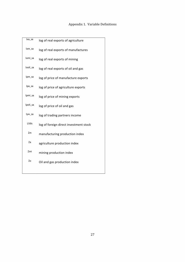
distinguished periods under study. Table 1 lists all variables used in the estimation.

Table 2 explains abbreviations for each of variables used in the estimations.

Export (X)

Export variable is calculated as export value deflated by export price index. Indonesian

export data is available in value and volume at 6 digits SITC revision 1 for series 1975-‐

1978, at 7 digits SITC revision 2 for series 1979-‐1988, and 8 digit SITC revision 3 for

series 1989-‐20083. The challenge is to find the appropriate deflator for the dependent

variable as export price index is non-‐existence for Indonesia. Using export volume index

as the dependent variable is also explored.

Export Price (Px)

3

6

Indonesia is among countries which does not record and/or publish export price in its

export data while export price is a crucial part of the econometric estimation for this

Chapter. There are few alternatives proxies for export price, among others are unit

value index and wholesale price index. None of these proxies are perfect measure for

export price. However, earlier researches are employing the two options whenever

price index is not available. Kravis and Lipsey (1974) criticize the use of unit value

indexes. Shiells (1991) however, finds that using unit value indexes does not greatly

affect estimated import demand elasticities, by comparing export unit value and export

price index compiled by the US Bureaus of Labor in estimating import demand

elasticities. While, whole sale price index is not available at sectoral and subsector level

in Indonesian, employing export unit value index as deflator and proxy for export price

variable is the only feasible option. Export unit value is calculated by dividing the value

of exports by the physical quantities of exports at the most disaggregated level.

While export unit value is used as deflator for export value and own price proxy in

estimating agriculture, manufacturing, mining and non-‐oil exports, in estimating oil

exports, oil price index from IMF IFS commodities price is used

(http://www.imfstatistics.org.virtual.anu.edu.au/imf/)

World Export Price (Pw)

World export price index is proxied by world export price index available from IMF

International Financial Statistics (http://www.imfstatistics.org.virtual.anu.edu.au/imf/).

Domestic Price (Pd)

Domestic price is proxied by wholesale price index, measured in US$ (CEIC

databaseAsia, 2010).

Trading partners’ income

Real income in importing countries is calculated as weighted real income of eight major

trading partners which accounted about 65 percent of Indonesia total exports (Japan,

US, Singapore, Korea, India, the Netherlands, Australia and United Kingdom). The

weights are 0.36 for Japan, 0.19 for US, 0.15 for Singapore, 0.13 for Korea, 0.06 for India,

0.04 for the Netherlands, 0.05 for Australia and 0.03 for United Kingdom. A number of

previous studies use world income as an explanatory variable including Goldstein and

Khan (1978) instead of trading partners’ income. However in this exercise, trading

7

partners’ income is used only trading partners’ income based on the rationale that they

are the most relevant to be included in the equations as in Athukorala and Suphacalasai

(2004) and Jongwanich (2009).

Domestic production (Z)

Due to unavailability of domestic production capacity data, following Jongwanich (2009)

domestic production capacity is proxy by Hodrick Prescott filtered manufacturing

production index for the manufacturing sector, agriculture sector value index GDP for

agriculture, oil and gas value index of GDP for oil and gas and mining GDP value index

for GDP.

Foreign Direct Investment (FDI)

For many countries, FDI is an important component in determining the supply side of

exports. UNCTAD (2010) reports Indonesia’s FDI inflows is about 3.1 of total gross fixed

capital formation on average for the period 1995-‐2005 and about 18 percent of GDP in

2007 (www.unctad.org.sections/dite_dir/docs/wir10_fs_id_en.pdf). It also reports the

share double in the period 2007-‐2008. The importance role of FDI in Indonesian export

activities are also shown in earlier studies (Sjoholm, 2003 and Ramstetter and Takii,

2005).

FDI stock is used as one of the explanatory variable in the estimation. The stock is

calculated using 1970 as the basis year and adding up the quarterly flow data from the

Balance of Payment to build the quarterly series.

All variables used in the estimation are in logarithm form and seasonally adjusted,

except for production capacity. Apart from the structure variable mentioned above,

dummy variables will be introduced to the oil boom period, trade liberalization period

of 1985 onwards and the 1997-‐1998 Asian crisis periods and the post crisis period.

EXPORT UNIT VALUE CALCULATION

The most challenging issues in the econometric estimation for this paper is getting the

data right, export deflator and export price in particular. The challenge lies in the

sectoral analysis. For Indonesia, published aggregated sectoral measures for exports are

non-‐existence. The Central Board of Statistics (CBS) collects export data from the

Custom Office, at 9 digit level HS/8digit SITC revision 3 for series 1989-‐2008, at 7digits

8

SITC revision 2 for series 1979-‐1988 and 6 digits SITC revision 1 for series 1975-‐1978.

The data is tabulated monthly, by ports of exportation and destinations, in terms of

value and volume. However, it does not record export price.

Consequently, the challenge in the estimating export demand and supply function is

finding the correct deflator for real export value or calculating the volume index if one

wants to use real export value as dependent variable as in this case, especially at

sectoral level. At aggregate level (total exports), IMF does publish export unit value.

Another possibility is to use the CBS whole sale price index (wpi). However this also

comes in aggregated (total and non oil export category) rather than sectoral.

Given the non-‐existence of export price data and export volume index at sectoral level,

which is crucial for the estimation, a few alternatives are available4. First is to use

weighted average of import price index of the major trading partners. James (2000) uses

US import price index as the deflator for Indonesian exports. However, one weakness of

this method is he differences in composition between Indonesian export and the trading

partner’s imports. Second is to use export unit value calculated from the most

disaggregated data (Shiells, 1991). Third is using the GDP sectoral deflator. However,

none of the above provides perfect measure for export price index.

The first proxy, using trading partners import price is rather crude and depends on the

availability of data. The best that we can get is the US, Japan and Korea import price

indexes as proxies. While the second proxy will be a tedious tasks as it involves data

cleaning (Shiells, 1991). In addition, for the case of Indonesia in particular as Rosner

(2000) pointed out a significant error in Indonesian export data, the quantity data in

particular an extra work in data cleaning is needed. The third proxy is the easiest,

however it does not reflect export price correctly. I compare the GDP deflator and

export unit value and found that GDP deflator does follow similar pattern of export unit

value.

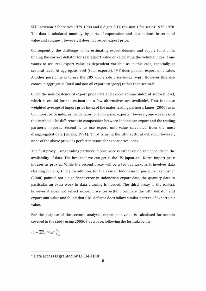
For the purpose of the sectoral analysis, export unit value is calculated for sectors

covered in the study using 2005Q3 as a base, following the formula below:

4 Data access is granted by LPEM-‐FEUI

9

where Pi is export unit value index of commodity i at the most disaggregated level,

, Pit is export unit value of commodity i in period t and Pio is export unit

value of commodity i in period 0.

Prior to calculating unit value index, volume data is cleaned up. In data cleaning process,

value data is assumed correct. Rosner (2000) shows that value data in Indonesian

export database is much cleaner than volume data. To address the issues, the cleaning

up of volume data follows a simple rule. The steps taken are as follow:

1. Price for each of product category (SITC7 digit for data in 1979-‐1988 period and

SITC 8 digit level for data in 1989-‐2009 period) is calculated by dividing value of

the particular category with its own volume.

2. Based on price, median of price for each year is calculated as a benchmark for

price movement in each year. The cleaning algorithm is as follows: if price in

particular month for particular commodity is x times of its respective year

median price or 1/x of its median price, price variable for that particular

commodity and month will be replaced by the median price

( . In the exercise,

different value of x is considered (3, 4, 5 and 10). It appears that using x=10 is

enough to adjust volume data entered wrongly, such as 0.1 written as 1.

3. Once price data is cleaned, volume data is cleaned using the new price data by

dividing value with the new adjusted unit value.

4. Due to different revisions of SITC used in the period of 1979 to 2008,

concordance is used to make the series comparable. However, the concordance

is only available at 4 and 5 digit level5

5. In calculating the index for 1979-‐2008, data are converted into SITC 4digits. This

implies for a longer time-‐span series (1979-‐2008), the measurement bias for

export unit value will be larger than the shorter time-‐span series (1989-‐2008).

5

http://unstats.un.org/unsd/trade/conversions/HS%20Correlation%20and%20Conver

sion%20tables.htm.

10

6. The calculated unit value index is compared with export unit value index for

total export published by CBS.

7. Further refinement is imposed to series in 1986 and 1988 due to extremely

price overshoot

ESTIMATION

One important consideration in modern time series analysis is stationarity of the data. A

series is considered to be stationary if it has constant mean, constant variance and

covariance (Asteriou and Hall, 2007). A random walk such as is non

stationary as the variance increased overtime. It is common to refer to stationary series

as integrated of order zero, or I (0), while non-‐stationary series is often referred as

integrated of order one or I (1) and series that is non-‐stationary at its first difference is

called integrated of order two, or I (2). Standard OLS will be valid on stationary series.

However, it will be spurious on I(1) or I(2) series. Granger and Newbold (1974) showed

that spurious regression from non-‐stationary data gives invalid t-‐test and F-‐test. Philips

(1986) showed that t-‐test and F test of spurious regression is getting larger as sample

size larger, the Durbin-‐Watson is approaching zero and R2 is approaching one. The

problem of spurious regression in time series analysis using macroeconomic data is

quite obvious as macroeconomic data are likely to contain unit roots, i.e. non-‐stationary.

Nelson and Plosser (1982) assessed 14 macroeconomic variables and found that 13 out

of 14 macroeconomic variables are non-‐stationary.

In recent times, there have been a number of methods can be employed for stationarity

test, also known as unit root test. The Dickey Fuller procedures have stood the test of

time as robust tools that appear to give good results over a wide range of application

(Greene, 2008, p 753).

11

COINTEGRATION

Economic theory suggests that exports have strong correlation with relative price,

income and production capacity (Goldstein and Khan,1985). Engle (1983) shows that

two or more of the non-‐stationary series when combined together might establish long

run relationship that eliminate the nonstationarity of the series. Cointegration test

needs to be carried out to confirm the relationship among the variables in equation (3).

There has been a number of cointegration test procedure, the Engle and Granger two

steps procedures (Engle and Granger, 1987), stochastic common trend of Stock and

Watson (1993) and system based reduced rank of Johansen (Johansen, 1991, 1995).

However, those methods are dealing with I(1) variables.

Given that the unit root test indicating that some of the series are I(0) and others are

I(1), the conventional cointegration test such Engle-‐Granger two steps procedure (Engle

and Granger 1983), Stock and Watson dynamic ordinary least square (1993) or the

Johansen method (Johansen 1988, 1991) would not be appropriate as those method

required all the series to be I (1).

Pesaran, Shin and Smith (2001) established an alternative method on testing the

cointegration for cases involving I(0) and I(1) variables. The statistic underlying the

Pesaran-‐Shin-‐Smith (PSS) procedure method is Wald test or F statistic in generalised

Dickey Fuller type regression to test the significance of lagged levels of variables in a

conditional unrestricted equilibrium error correction model (ECM) (Pesaran, et al, 2001,

p 290). They developed two sets of asymptotic critical value. The first set assumes all

regressors are I(0) series while the second set assumes all the regressors are I(1). The

two sets of the critical values are then the critical value bounds for all classifications of

the regressors. The decision rule is if the F-‐ test from Wald test falls outside the critical

value conclusive inference can be made without needing to know the

integration/cointegration of the series. However, if the F test falls within the lower and

upper bound, a conclusive inference cannot be made until the order of integrations of

the independent variables can be determined (Pesaran et al, 2001 p 290).

12

The Pesaran bound test is computed based on an estimate of unrestricted error

correction models (UECM) or error correction version of autoregressive distributed lag

(ARDL) model using ordinary least square estimator (Pesaran et al, 2001, p 293)

For the purpose of this research, the UECM will be in the form below

(4)

where D represents the first difference operator (Xt-‐Xt-‐1), l is the lag length, u is the white

noise and normally distributed residuals. Based on the UECM, the bound test is

performed with null hypothesis of no cointegration among the regressors (H0:

b6=b7=b8=b9=b10=0) using Wald test. The Wald test is compared to the bound critical

value (Table CI(i)-‐CI(v) in Pesaran 2001, page 300-‐301). If the Wald test statistics is

greater than the upper bound of the critical value, the null hypothesis can be rejected. If

it is smaller than the lower bound of the Pesaran critical value, the null hypothesis

cannot be rejected. However, if the F test falls within the lower and upper bound, a

conclusive inference cannot be made until the order of integrations of the independent

variables can be determined.

Lag-‐length Selection, General to Specific Method and Diagnostic Test

In estimating the UECM as in equation (4) above, lag length is chosen based on Akaike

Information Criteria (AIC) and Bayesian Schwarz Information Criteria, as well the

Breusch and Godfrey’s LM test for serial correlation. The first difference explanatory

variables which are not statistically significant are dropped successively based on

general to specific method (Hendry, et al, 1984). Diagnostic test is conducted to check

the robustness and stability of the model chosen: LM test for serial correlation and

RESET test for misspecification in the functional form.

13

RESULTS

COINTEGRATION TEST

The Pesaran bound test result as in Table 5 shows that exports and its explanatory

variables are cointegrated at 5 % significant level in all sectors, except oilandgas sector

which is significant at 10%.

LONG RUN DETERMINANTS OF EXPORTS Total Exports

The long run equilibrium estimates for total export as in Table 5 shows that own price

(px), production capacity (z) and stock of foreign direct investment (fdi) are statistically

significant variables while trading partner’s income (yw) is found to be statistically

insignificant. Dummy variable POST is found to be statistically significant, indicating

export in the post reform period is higher. This result supports Athukorala conjecture

that supply side rather than demand side are the more relevant determinants of

Indonesian export performance.

From the UECM equation for total export , the cointegration relationship is as follow:

(5)

For the cointegration relationship as above, export price elasticities and income

elasticities are computed as , and . Using

total exports data, export price elasticity is relatively low, around -‐0.34.

Sectoral Findings Manufacture

The result for manufacturing as in Table 6 also shows world income is being statistically

insignificant. FDI appears to be a significant variable for Indonesian manufacturing

exports. Dummy variable post is statistically significant indicating manufacturing

14

exports is higher in the post reform period. Similar to total exports, export price

elasticity for manufacturing exports is also low, -‐0.31.

Agriculture

Agriculture export is relatively homogenous. Consequently, export demand and supply

model applied to agriculture is different from the above model. Following Goldstein and

Khan (1986), export demand and supply function for homogenous products is as follow:

(6)

(7)

Where Xd is export demand, Xs is export supply, P is price of agriculture product, Y is

world income and Z is production capacity.

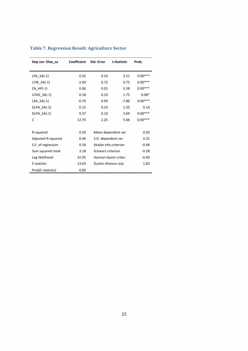
Table 7 shows econometric results for agriculture exports. It shows price, income,

production capacity and FDI are significant explanatory variable for agriculture export.

However, price is positively correlated with export, with price elasticity of + 0.5 which

means a 1 percent increase in export price increase Indonesian export by 0.5 percent.

This might be a reflection of quality improvement of Indonesian agriculture exports.

Variable world income also revealed different sign from manufacturing. For agriculture

export, income is negatively correlated to exports . A 1 percent increase in trading

partner’s income reduce exports by 3.8 percent. This might be related to the more

stringent WTO compliance-‐non tarrif barriers such sanitary and phytosanitary

requirements in higher income countries. To take into account the effect of recent

commodity boom, dummy variable commboom is included, however it is statistically

insignificant, while the result for the rest of the coefficients are relatively similar.

Oil and Gas

Similar to agriculture, oil and gas sector is considered to be homogenous. Economic

result as in Table 8 shows income is the only significant variable in explaining export

performance of this sector.

15

CONCLUSION

Indonesia has been embarking on substantive economics reform since 1985. It was severely hit by

1997/1998 Asian financial crisis. In the post crisis period, Indonesian export has been slowing down.

Earlier study indicates that the slowing down of exports is mainly due to supply side problem.

Time series analysis using Pesaran bound testing on total exports, manufacturing exports, oil exports

and non-oil exports for the period of 1976-2008 shows export price, production capacity and foreign

direct investment (FDI) stock are significant variables in explaining Indonesian long term export

performance. This supports earlier conjecture that Indonesian export performance is supply driven.

This paper also estimates price elasticity of export, one estimates for long term own price elasticity of

exports is -0.34 for total exports, and -0.31 for manufacturing. In contrast, price is positively correlated

and income is negatively correlated with agriculture export. Similar to manufacturing, FDI is

statistically significant variables. In conclusion, apart from price, it appears that supply side variables

are also very important in determining Indonesia’s export performance.

16

TABLES AND FIGURES Figure 1. Indonesian Share in World Export 1970-2008 (in percent)

Source. Comtrade, author’s calculation

Figure 2. Export Growth: Indonesia and World

17

Figure 3. Export Growth 1975-2008: Regional Comparisons

Figure 4. Sectoral composition

18

Figure 5. Export Growth: Manufacturing

19

Table 1. Variables and Data

Variable Calculation Source Export Real Export Value=export value (US$)/export price

index (US$) Export value from CBS and export price index from IFS

Prices Own price is proxied by export unit value calculated by dividing value to volume at 4 digits level SITC. World price for total export is proxied by world export unit value from IMF IFS. Domestic price is proxied by sectoral whole sale price index

CBS and IFS

Trading Partner Income

The eight trading partner’s real GDP weighted by export share

Real GDP from IFS at quarterly bases except for India, Singapore and Netherlands, where some points at the beginning periods are converted from annual data

Production Capacity

Industrial Production Index and GDP sectoral production index

CBS

The data are mainly at quarterly basis. There are some points at the beginning periods where data only available at annual basis. For these cases the annual data are converted using linear transformation.

Foreign Direct Investment

Foreign Direct Investment Stock The stock is calculated using 1970 as the basis year and adding up the quarterly flow data from the Balance of Payment to build the series

Oil oil=1 for years before 1980 Dummy variable to capture the oil boom period

Pre pre =1 for years before 1985 Dummy variable to capture periods before reform

Post post=1 for years after 1986 Dummy variable to capture periods after reform

Crisis Dummy variable to capture crisis period. Crisis=1 for years 1997 and 1998, = 0 otherwise

Commboom

Dummy variable for commodity boom year. Commboom=1 for period of 2006 to 2007,= 0 otherwise

20

Table 2 ADF Unit Root Test*

Variables ADF test Lag length

Test type Order of Integration

Level -‐2.061312 1 constant and trend lxa_sa

First Difference -‐2.061312 0 constant

I(1)

Level -‐0.617606 0 constant and trend lxm_sa


I(1)

Level -‐3.987533 1 constant and trend lxmi_sa


I(0)

Level -‐3.558535 4 constant and trend lxoil_sa


I(0)

Level -‐3.23949 3 constant lpm_sa


I(1)

Level -‐2.080458 0 constant and trend lyw_sa


I(1)

Level -‐4.104518 8 constant and trend Lfdis


I(0)

Level -‐3.652353 4 constant and trend Zm


I(0)

Level -‐3.635465 3 constant and trend Za


I(0)

Level -‐1.563828 2 constant and trend Zmi


I(1)

Level -‐2.205381 1 constant and trend Zo


I(1)

*variable with extension _sa is seasonally adjusted using X12 method

**see Appendix 1 for variable definition

21

Table 3. Inverse Demand Estimation

Dependent variable: Dlpx_sa

Coefficient Std. Error t-Statistic Prob.

C -1.34 0.76 -1.76 0.08

LXT_SA(-1) 0.09 0.06 1.56 0.12

LPW_SA(-1) 0.13 0.07 1.78 0.08

LYW_SA(-1) -0.19 0.13 -1.48 0.14

LPX_SA(-1) -0.02 0.03 -0.58 0.56

DLXT_SA(-1) -0.02 0.10 -0.24 0.81

DLXT_SA -0.66 0.07 -9.27 0.00

DLPW_SA(-1) 0.37 0.31 1.20 0.23

DLPW_SA 0.87 0.32 2.71 0.01

DLYW_SA(-1) 2.37 0.91 2.59 0.01

DLYW_SA 1.28 0.93 1.37 0.17

DLPX_SA(-1) -0.04 0.10 -0.39 0.70

R-squared 0.62 Mean dependent var 0.01

Adjusted R-squared 0.58 S.D. dependent var 0.10

S.E. of regression 0.07 Akaike info criterion -2.46

Sum squared resid 0.47 Schwarz criterion -2.18

Log likelihood 154.76 Hannan-Quinn criter. -2.35

F-statistic 15.65 Durbin-Watson stat 2.03

Prob(F-statistic) 0.00

22

Table 4. Bound Test Results

Sector Wald Test Total

7.80 Agriculture

12.69 Manufacture

10.89 Oil/Gas

3.50 Critical Value for Bound Test (Pesaran et, al 2001, p 300) no intercept and no trend :[2.14 , 3.34] at 5% and [1.90, 3.01] at 10% intercept and no trend :[2.62 , 3.79] at 5% and [2.26 , 3.35] at 10%

23

Table 5. Regression Results for Total Exports

Dep var: Dlx_sa Coefficient Std. Error t-‐Statistic Prob.

C 8.72 1.36 6.42 0.00 ***

LPX_SA(-‐1) -‐0.19 0.06 -‐3.42 0.00 ***

LYW_SA(-‐1) 0.18 0.14 1.29 0.20

LPD_SA(-‐1) 0.09 0.08 1.10 0.27

Z_HP(-‐1) 0.00 0.00 4.11 0.00 ***

LFDIS_SA(-‐1) 0.12 0.05 2.26 0.03 **

LXT_SA(-‐1) -‐0.56 0.08 -‐6.64 0.00 ***

DLPX_SA(-‐3) 0.30 0.08 3.68 0.00 ***

DLPX_SA -‐0.62 0.06 -‐9.81 0.00 ***

DZ_HP(-‐1) 0.08 0.03 2.66 0.01 **

DLXT_SA(-‐3) 0.40 0.08 5.17 0.00 ***

DLFDIS_SA -‐0.64 0.24 -‐2.69 0.01 **

DLPD_SA 0.12 0.06 1.95 0.05 *

PRE 0.01 0.04 0.33 0.74

POST 0.12 0.04 2.96 0.00 ***

CRISIS 0.01 0.04 0.16 0.88

R-‐squared 0.78 Mean dependent var 0.01

Adjusted R-‐squared 0.73 S.D. dependent var 0.11

S.E. of regression 0.05 Akaike info criterion -‐2.79

Sum squared resid 0.27 Schwarz criterion -‐2.26

Log likelihood 179.78 Hannan-‐Quinn criter. -‐2.58

F-‐statistic 15.28 Durbin-‐Watson stat 2.00

Prob(F-‐statistic) 0.00

*** 1% significant level

** 5 % significant level

* 10 percent significant level

24

Table 6. Regression Result for Manufacturing Exports

Dep var: Dlxm_sa Coefficient Std. Error t-‐Statistic Prob.

LPM_SA(-‐1) -‐0.17 0.08 -‐2.17 0.032 **

LPD_SA(-‐1) 0.47 0.17 2.73 0.008 ***

LYW_SA(-‐1) 0.48 0.55 0.87 0.387

LFDIS_SA(-‐1) 0.33 0.17 1.92 0.058 *

LXM_SA(-‐1) -‐0.53 0.07 -‐8.07 0.000 ***

DLPM_SA(-‐3) 0.14 0.10 1.50 0.138

DLYW_SA(-‐2) 12.79 5.99 2.14 0.035 **

DLYW_SA -‐10.59 5.13 -‐2.07 0.042 **

C 2.24 1.13 1.98 0.051 ***

CRISIS 0.03 0.15 0.23 0.822

PRE -‐0.16 0.15 -‐1.05 0.295

POST 0.62 0.16 3.98 0.000 ***



S.E. of regression 0.28 Akaike info criterion 0.40

Sum squared resid 7.22 Schwarz criterion 0.71

Log likelihood -‐8.84 Hannan-‐Quinn criter. 0.52



*** 1% significant level

** 5 % significant level

* 10 percent significant level

25

Table 7. Regression Result: Agriculture Sector

Dep var: Dlxa_sa Coefficient Std. Error t-‐Statistic Prob.

LPA_SA(-‐1) 0.35 0.10 3.51 0.00***

LYW_SA(-‐1) -‐2.69 0.72 -‐3.75 0.00***

ZA_HP(-‐1) 0.06 0.01 5.58 0.00***

LFDIS_SA(-‐1) 0.18 0.10 1.75 0.08*

LXA_SA(-‐1) -‐0.70 0.09 -‐7.86 0.00***

DLPA_SA(-‐2) 0.15 0.10 1.50 0.14

DLPA_SA(-‐1) 0.37 0.10 3.69 0.00***

C 12.70 2.25 5.66 0.00***



S.E. of regression 0.18 Akaike info criterion -‐0.48

Sum squared resid 3.18 Schwarz criterion -‐0.28

Log likelihood 32.95 Hannan-‐Quinn criter. -‐0.40



26

Table 8. Regression Result for Oil Exports

Dep var: Dlxoil_sa Coefficient Std. Error t-‐Statistic Prob.

LPOIL_SA 0.045 0.237 0.190 0.850

LYW_SA(-‐1) 1.174 0.702 1.671 0.098 *

ZO(-‐1) 0.006 0.004 1.594 0.115

LFDIS_SA(-‐1) -‐0.138 0.207 -‐0.663 0.509

LXOIL_SA(-‐1) -‐0.363 0.075 -‐4.844 0.000 ***

DLPOIL_SA -‐1.591 0.379 -‐4.197 0.000 ***



S.E. of regression 0.514 Akaike info criterion 1.568

Sum squared resid 23.246 Schwarz criterion 1.731

Log likelihood -‐67.713 Hannan-‐Quinn criter. 1.634

Durbin-‐Watson stat 2.195

27

Appendix 1. Variable Definitions

log of real exports of agriculture lxa_sa

log of real exports of manufactures lxm_sa

log of real exports of mining lxmi_sa

log of real exports of oil and gas lxoil_sa

log of price of manufacture exports lpm_sa

lpa_sa log of price of agriculture exports

lpmi_sa log of price of mining exports

lpoil_sa log of price of oil and gas

log of trading partners income lyw_sa

log of foreign direct investment stock Lfdis

manufacturing production index Zm

agriculture production index Za

mining production index Zmi

Oil and gas production index Zo

28

Appendix 2. Data Series

LPX=Log of Total Export Unit Value Index LPX_SA=Log of Total Export Unit Value Index Seasonally Adjusted

LPW= log of world price index LPW_SA= log of world price index_ seasonally adjusted

lpm=log of manufacturing export price lpmi=log of mining export price

lpa=log of agriculture export price lpoil=log of oil export price

29

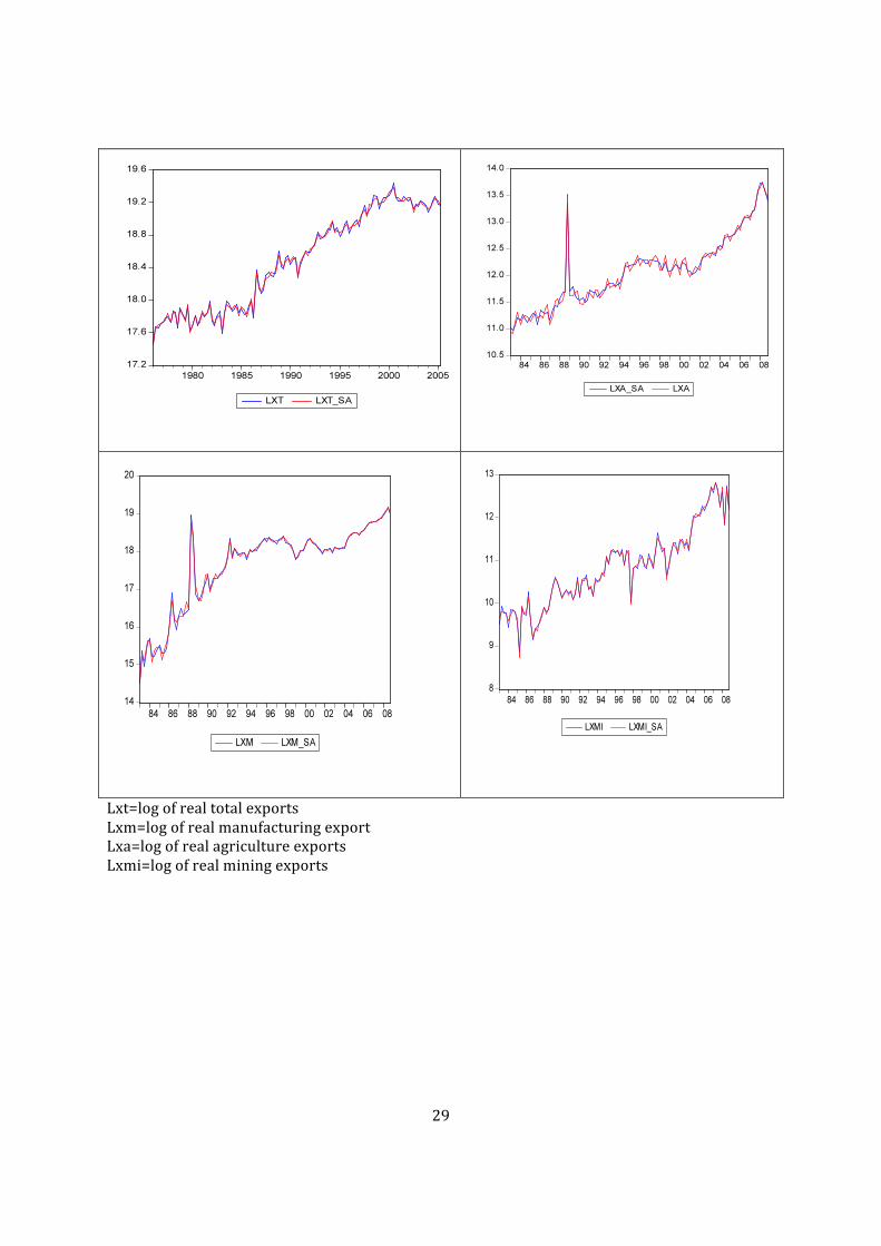
Lxt=log of real total exports Lxm=log of real manufacturing export Lxa=log of real agriculture exports Lxmi=log of real mining exports

31

Za=agriculture production index Zmi=mining production index

Zm=manufacture production index Zo=oil production index

32

References

ASTERIOUS, DIMITRIOS AND STEPHEN HALL, 2007, APPLIED ECONOMETRICS: A MODERN APPROACH,

PALGRAVE MACMILLAN

ATHUKORALA, P 2004, ‘POST-CRISIS EXPORT PERFORMANCE IN THAILAND’, ASEAN ECONOMIC

BULLETIN, 21(1), PP. 19-36.

ATHUKORALA, P 2006, POST-CRISIS EXPORT PERFORMANCE: THE INDONESIAN EXPERIENCE

IN REGIONAL PERSPECTIVE, BULLETIN OF INDONESIAN ECONOMIC STUDIES, VOL. 42, NO. 2, 2006:

177–211

ATHUKORALA, P. 1998 ‘EXPORT RESPONSE TO LIBERALIZATION: THE SRI LANKAN EXPERIENCE’

HITOTSUBASHI JOURNAL OF ECONOMICS, VOL 39 NO 1 JUNE 1998

ATHUKORALA, P.& RIEDEL J. 1994, ‘DEMAND AND SUPPLY FACTORS IN THE DETERMINATION OF NIE

EXPORTS: A SIMULTANEOUS ERROR CORRECTION MODEL FOR HONGKONG: A COMMENT’, THE ECONOMIC

JOURNAL, VOL 102, NO 415, PP.1467-1477,

ATHUKORALA, P., RIEDEL, J., 1991, ‘THE SMALL COUNTRY ASSUMPTION: A REASSESSMENT WITH

EVIDENCE FROM KOREA’. WELTWIRTSCHAFTLICHES ARCHIV 127 _1., PP.138–151.

BALASA, B., VOLOUDAKIS, FYLAKTOS & SUH 1989, ‘THE DETERMINANTS OF EXPORT SUPPLY AND

EXPORT DEMAND IN TWO DEVELOPING COUNTRIES: GREECE AND KOREA’, INTERNATIONAL ECONOMICS

JOURNAL, VOL 3, NUMBER 1, 1989

BALASSA, B (1979) EXPORT COMPOSITION AND EXPORT PERFORMANCE IN THE INDUSTRIAL COUNTRIES,

1953-1971, REVIEW OF ECONOMICS AND STATISTICS LXI::604-607

BARDSEN, G (1989), ESTIMATION OF LONG RUN COEFFICIENTS IN ERROR CORRECTION MODELS,

OXFORD BULLETIN OF ECONOMICS AND STATISTICS, 51:345-50

EDWARDS, LAWRENCE AND PHIL ALVES (2006), SOUTH AFRICA'S EXPORT PERFORMANCE:

DETERMINANTS OF EXPORT SUPPLY, SOUTH AFRICAN JOURNAL OF ECONOMICS VOLUME 74, ISSUE

3, PAGES 473–500, SEPTEMBER 2006

ENDERS, W. 1994, APPLIED ECONOMETRIC TIME SERIES, WILEY&SONS, CANADA

ENGLE AND GRANGER (1987)

33

GOLDSTEIN, M. & KHAN M.S. 1986, ‘TRADE DEMAND AND SUPPLY’, IN HANDBOOK OF INTERNATIONAL

ECONOMICS, VOLUME 2, 1986

GOLDSTEIN, M.& KHAN M.S. 1978, ‘THE SUPPLY AND DEMAND FOR EXPORTS: A SIMULTANEOUS

APPROACH’, THE REVIEW OF ECONOMICS AND STATISTICS, VOL 60, NO 2 (APRIL, 1978), PP.275-286

GRANGER AND NEWBOLD (1974), SPURIOUS REGRESSIONS IN ECONOMETRICS, IN SPECTRAL ANALYSIS,

SEASONALITY, NONLINEARITY, METHODOLOGY AND ..., VOLUME 1

GREENE, W.H 2008, ECONOMETRIC ANALYSIS, PEARSON INTERNATIONAL, NEW JERSEY, USA

HENDRY ET AL (1984), DYNAMIC SPECIFICATION IN Z GRILICHES AND MD INTRILOGATOR (EDS),

HANDBOOK FO ECONOMETRICS, VOL 2. NORTH HOLLAND, AMSTERDAM

HODRICK, ROBERT J. AND EDWARD C. PRESCOTT, (1997), POSTWAR US BUSINESS CYCLES: AN

EMPIRICAL INVESTIGATION, JOURNAL OF MONEY,CREDIT ANDBANKING VOL 29, NO 1, FEBRUARY 1997

JOHANSEN (1991)

JOHANSEN (1995)

JONGWANICH, J. (2009) "DETERMINANTS OF EXPORT PERFORMANCE IN EAST AND SOUTHEAST ASIA."

WORLD ECONOMY 33(1): 20-41.

M. HASHEM PESARAN, YONGCHEOL SHIN, RICHARD J. SMITH (2001), BOUNDS TESTING APPROACHES TO

THE ANALYSIS OF LEVEL RELATIONSHIPS, JOURNAL OF APPLIED ECONOMETRICS SPECIAL ISSUE: IN

MEMORY OF JOHN DENIS SARGAN 1924–1996: STUDIES IN EMPIRICAL MACROECONOMETRICS, VOLUME

16, ISSUE 3, PAGES 289–326, MAY/JUNE 2001

MAGEE, C. S. P.& MAGEE S.P. 2008, ‘THE UNITED STATES IS A SMALL COUNTRY IN WORLD TRADE’ ,

REVIEW OF INTERNATIONAL ECONOMICS, VOLUME 16 ISSUE 5 , PAGES 817 - 1043

MARJIT SUGATA AND AJITAVA RAYCHAUDHURI (1997), INDIA’S EXPORT: AN ANALYTICAL STUDY,

OXFORD UNIVERSITY PRESS, DELHI

NELSON AND PLOSSER (1982)

PANAGARIYA, A, SHAH S. & MISHRA D. 2001, ‘DEMAND ELASTICITIES IN INTERNATIONAL TRADE: ARE

THEY REALLY LOW’, JOURNAL OF DEVELOPMENT ECONOMICS, VOL 64, 2001

PHILIPS (1986)

34

RIEDEL, J. 1988, ‘THE DEMAND FOR LDC EXPORTS OF MANUFACTURES: ESTIMATES FROM HONGKONG’,

THE ECONOMIC JOURNAL, VOL 98, NO 389, PP.138-148

ROSNER, L.PETER (2000), INDONESIA’S NON-OIL EXPORT PERFORMANCE DURING THE ECONOMIC

CRISIS: DISTINGUISHING PRICE TRENDS FROM QUANTITY TRENDS, BULLETIN OF INDONESIAN ECONOMIC

STUDIES 36:61-95

SHIELLS, CLINTON (1991), ERRORS IN IMPORT-DEMAND ESTIMATES BASED UPON UNIT VALUE

INDEXES, THE REVIEW OF ECONOMICS AND STATISTICS, VOLUME 873, NO2, PP 378-382

SIREGAR, R.& RAJAN, R. 2004, ‘IMPACT OF EXCHANGE RATE VOLATILITY ON INDONESIAN’S TRADE

PERFORMANCE IN THE 1990S’, JOURNAL OF JAPANESE AND INTERNATIONAL ECONOMICS, 18 (2004)

218-240

STOCK, JAMES H AND MARK W. WATSON (1993), A SIMPLE ESTIMATOR OF COINTEGRATING VERCTOS

IN HIGHER ORDER INTEGRATED SYSTEMS, ECONOMETRIICA 61(4):783-820

STOCK, JAMES H AND MARK W. WATSON (2007), INTRODUCTION TO ECONOMETRICS, PEARSON

EDUCATION

WARR, P.G.& WOLLMER,F.J 1997, ‘TESTING THE SMALL-COUNTRY ASSUMPTION: THAILAND'S RICE

EXPORTS’, JOURNAL OF THE ASIA PACIFIC ECONOMY, 1469-9648, VOLUME 2, ISSUE 2, 1997, PAGES

133 – 143

titik anas determinants of exports - crawford school of ... ·...

Documents