title effective demand and national income : a

Title Effective Demand and National Income : A Microeconomics of the IS-LM Analysisand its Application to the Stagnation of the Japanese Economy

Sub TitleAuthor 大山, 道廣(OHYAMA, MICHIHIRO)

Publisher Keio Economic Society, Keio UniversityPublication year 2004

Jtitle Keio economic studies Vol.41, No.2 (2004. ) ,p.1- 23 Abstract

NotesGenre Journal ArticleURL https://koara.lib.keio.ac.jp/xoonips/modules/xoonips/detail.php?koara_id=AA002

60492-20040002-0001

慶應義塾大学学術情報リポジトリ(KOARA)に掲載されているコンテンツの著作権は、それぞれの著作者、学会または出版社/発行者に帰属し、その権利は著作権法によって保護されています。引用にあたっては、著作権法を遵守してご利用ください。

The copyrights of content available on the KeiO Associated Repository of Academic resources (KOARA) belong to the respective authors, academicsocieties, or publishers/issuers, and these rights are protected by the Japanese Copyright Act. When quoting the content, please follow theJapanese copyright act.

Powered by TCPDF (www.tcpdf.org)

http://www.tcpdf.org

KEIO ECONOMIC STUDIES 41(2), 1-23 (2004)

EFFECTIVE DEMAND AND NATIONAL INCOME: A MICROECONOMICS

OF THE IS-LM ANALYSIS AND ITS APPLICATION TO THE

STAGNATION OF THE JAPANESE ECONOMY

Michihiro OHYAMA

Department of Economics, Toyo University, Tokyo, Japan Keio University, Tokyo, Japan

First version received April 2005; final version accepted July 2005

Abstract: This paper develops a simple microeconomics of the 1 S-LM analysis with the intention of understanding controversies about the long-term stagnation of the

Japanese economy and suggesting some remedies. Using an extended two-period model

of the representative consumer with the Robertsonian consumption lag, I derive the Keynesian consumption function and liquidity function and formulate the I S-LM equi-librium on that basis. It contains the Keynes—Hansen 45 degree-line model of effective demand as a special case where the consumer has no liquidity preference, and the econ-

omy is caught in the zero-interest rate liquidity trap. The model supports the Mone-tarist's view that it is impossible to achieve full employment without providing enough

money for transactions. It also endorses the Keynesian policy of fiscal expansion in the short run and structural reforms conducive to improving the public's expectations of fu-ture income in the long run as effective remedies for underemployment due to deficient

aggregate demand. (JEL El 0 E21 E24)

Key words: Consumption; Liquidity Preference; Liquidity Trap; Multiplier. The Japanese Economy.

JEL Classification Number:

1. INTRODUCTION

As the Japanese economy suffered from extremely slow or even negative growth

and increasing unemployment for more than a decade since the collapse of the Bub-ble around 1992, policy makers and commentators were apparently divided into three distinct camps, Structuralists, Inflationisits, and Keynesians with respect to their diag-noses and policy proposals for Japan's conomic trouble. The Structuralists , adopted by the Koizumi cabinet of Japan, pointed to government budget deficits, banking sys-tem, social security system and anachronistic regulations on economic activities as the major factors responsible for the long stagnation and argued for structural reforms as

E-Mail:

Copyright © 2004, by the Keio Econimic Society

1

2 KEIO ECONOMIC STUDIES

indispensable prerequisites for revitalization of the ailing economy. They regarded fis-cal and monetary stabilization policies as shortsighted and ineffective in view of the discouraging experiences in the troubled decade. Keynesians and Inflationists believed that the chronic deficiency of aggregate demand was the most important immediate cause of the depression and called for the continued execution of appropriate fiscal and monetary policies as measures inescapable for economic recovery, but their emphases were different. Naturally, Keynesians tended to support appropriately designed fiscal expansion or tax-cut as effective policy instruments to combat unemployment due to deficient demand. In contrast, Inflationists, e.g., Krugman (1998), advocated the cre-ation of long-run inflation by means of steady expansion of monetary base (the so-called inflation targeting policy).

What are their underlying economic models? Some extreme structuralists may be sympathetic to the neoclassical macroeconomic model in which the aggregate market economy behaves as if it were planned and foreseen by a rational individual possessing

perfect information about its structure and, therefore, any governmental stabilization policy is not just unnecessary and but also harmful. This model is, however, too un-real to be accepted by policy-minded economists even in the structuralist camp. The old IS-LM model seems to be still influential among practical economists belonging to the Inflationist and Keynesian camps, but it is no longer fully supported by aca-demics because of its lack of microeconomic foundations' . There are ceratainly some attempts by the New Keynesians, beginning with Kiyotaki and Blanc hard (1987) and Kiyotaki (1988), to provide various policy-oriented macroeconomic models with mi-croeconomic foundations.2 They typically introduce monopolistic competition among firms (or households) and invoke the existence of menu costs, or coordination failures among firms to justify government intervention (such as monetary expansion) in the market economy. The phenomenon of underemployment envisaged in these models is attributable to the assumption of monopolistic competition rather than to the deficiency of aggregate demand. They are perhaps far away from the view of the world entertained by practical present-day Keynesians as well as old Keynesians. Apparently, they are not designed to match the world of structuralists and inflationists either.

The present paper attempts to construct a new microeconomics of the IS-LM anal-

ysis focusing on the deficiency of aggregate demand as the culprit of economic de-pression and capable of embracing at least partially the views of all three camps of economists mentioned above. In this connection, we should note that Krugman (1998) also proposed a useful model of an aggregate Keynesian economy with a microeco-nomic foudation. His model is, however, too simple as a re formulation of the IS-LM model in its treatment of money, long-run expectations, and government to compare and discuss various policy measures. In this paper, we present an alternative and much

I For instance , see McCallum and Nelson (1999) for a review of the main criticisms of the IS-LM approach. Nevertheless, the I S-LM model is adopted as the main workhorse for the analysis and exposition

of macroeconomic phenomena in such relatively new and popular textbooks for undergraduate students as

Mankiw (1992) and Blanc hard (1997). 2 For a survey of the literature , see Silvestre (1993).

OHYAMA: EFFECTIVE DEMAND AND NATIONAL INCOME 3

more structured model consistent with the representative consumer's optimizing behav-ior. As a price of detailed analysis of the demand side of the economy , we simplify here the supply side of the economy abandaning the fill rationalization of the model . This setup not only follows the tradition of the 1 S-LM analysis but also reflects the widely

accepted observation that the long-term slump of the Japanese economy was partly at-tributable to its high saving rate or low propensity to consume . The structure and major conclusions of the paper are as follows.

In Section 2, we shall formulate the representative consumer's optimizing behavior in the economy in which money serves not only as a means of payment circulating from

producers to consumers and then from consumers back to producers with a one-period time lag as in the Robertsonian period analysiss but also as a store of value when bonds

(or loan contracts) are exposed to default risks as emphasized by Keynes (1936). In Section 3, we shall derive the "Keynesian" consumption function and liquidity prefer-

ence function which depend negatively on the nominal rate of interest, and positively on current disposable national income, financial wealth and the consumer's expecta-tions of future income flows. The last factor reflects the consumer's perception of job

opportunities, national productive capacity and social security system in the future . It is important especially because Structuralists, Inflationists and Keynesians all agreed that the public's low expectations concerning future income was substantially responsible for the stagnation of the Japanese economy. Section 3 will then define the market equi-

librium of the economy and lay a microeconomic foundation of the I S-LM analysis . Section 4 will be devoted to the analysis of monetary and fiscal policies and Section 5 to

the discussion of other disturbances exogenous to the model. The present mode] clearly supports the old Monetarist's view that it is impossible to achieve full-employment na-tional income without providing enough money for transactions . Also, it will show that monetary expansion by means of open market operation is not effective when the aggregate effective demand is extremely weak and the nominal interest rate is close to

zero as in the Japanese economy at the beginning of the 21 gt century. In order to boost the economy under such a circumstance, it is therefore necessary to adopt Keynesian

policies such as tax cut and government spending in the short run, and to carry out structural reforms conducive to improving the public's expectations of future income in the long run. The creation of inflation expectations by continued monetary expansion

la Krugman (1998) may also be helpful if it succeeds in increasing the present value of expected flows of future income.

In section 6. we shall consider the special case of the present model where there is

no demand for money as a store of value, or to put it differently, bonds are received to

be risk less. This is the so-called Monetarist case in which the LM curve becomes ver-tical. Rather surprisingly, it will turn out to replicate the simplest Keynesian model of effective demand as developed in Keynes (1936, Chapter 3) and illustrated by Hansen

(1953) when the economy is caught in the zero-interest liquidity trap. For instance, an increase in government spending will be shown to exert a positive multiplier effect on

3 Robertson (1926) .


national income without crowding out private expenditure. It differs, however, from the standard version of the Keynesian model in the sense that money is important here. The monetary authority must increase money supply either by open-market operation or by

money printing in order to realize the increase in national income. The usual exposi-tion of the Keynes—Hansen model ignores this monetary implication of fiscal policy. As long as money supply is increased by open market operation, all the results of com-

parative statics in the Keynes—Hansen model are valid in the present model including the balanced budget proposition that the fiscal multiplier is equal to unity in case of

tax-financed increase in the government spending. In case of money printing, however, the multiplier effects of autonomous spending will be enhanced and the balanced bud-

get multiplier will become greater than unity. In Section 7, we consider some dynamic implications of the present model allowing for statically rational income expectations and adjustment of the price level in response to the gap between full employment and

actual incomes. Finally, Section 8 concludes the paper by pointing out some limitations of the present analysis.

2. CONSUMPTION AND LIQUIDITY PREFERENCE

We consider an extended two-period economy in which there are many identical con-

sumers who behave as if they were one giant consumer. The representative consumer

plans to consume in the current period and also store some real purchasing power for future consumption without distinguishing consumption expenditures in different future

periods. Her income is paid in money every period in the form of wages, dividends and interest from her labor and capital (loan) services delivered in the preceding period. For simplicity and definiteness, let us assume that the representative consumer's utility

function at the beginning of period t is of the following log-linear form:

wt=lnCl+ -y)InRf+1+ylnLt, l>y,y>0.(1)

where Ct is real consumption in period t, Rt+l is the real purchasing power the con-sumer plans to hold at her disposal in period t + 1 for future consumption through

financial and non-financial arrangements (to be explained later), and Lt is the part of Rt+i she plans to store in the form of real cash balance.4 Note also that money plays a role as a store of value. Our interpretation of the money-in-utility assumption is quite

different from the usual explanation that money holding represents the utility derived from consumption in all future periods, or that it reduces implicit transactions costs.)

We take it to mean that there is some uncertainty about the real value of loan contract in view of possible default and parameter y reflects the consumer's evaluation of this uncertainty. The greater the value of y is, the greater her perception of or aversion to

4 When y = 0 , R,+t can be interpreted as the composite commodity of future consumption goods, given the expected rates of interest and inflation in future periods. See Hicks (1939), Mathematical Appendix.

5 For instance , see Nealy and Stiglitz (1983), or McCallum and Nelson (1999).


this uncertainty is.6 We believe that the present modelling of the consumer's behav-ior is one of the possible ways to formulate her intrinsic nearsightedness and bounded rationality.7 We assume that there is only one good called the "national product". Firms produce the national product using labor and capital stock and finance their investment (if any) by borrowing from consumers in each period. The government finances its expenditure by taxing consumers. For simplicity, the government is assumed here to keep balanced budget. The central bank is assumed to control money supply either by engaging in open market operation or by printing money at the beginning of each period. In case that the consumer is fully aware of her ownership of firms, the private loans cancel out each other. Here, the consumer is supposed to respect her interest income and distinguish it from her non-interest income consisting of wages and dividends. In the contempo-rary capitalism characterized by separation of ownership and management, the present assumption seems more natural.s At the beginning of each period, the consumer is sup-

posed to prepare money for consumption, tax payment and saving out of interest and non-interest money incomes obtained from firms as rewards to the services she deliv-ered in the preceding period and cash balances carried over from the preceding period. Thus, money serves as a means of payment as well. The consumer's consumption in

period t is constrained by

pt(C, + Ti) < pt-l Xi_1 + (1 + it-l)Ar-l + pt-l Lt-l — At — PtL, (2)

+AMt— AHt,

where pt and Ti denote the price level and tax payment (fixed in real value) in period t, pt_I and Xi_I the price level and non-interest real income in period t — 1, il_1 the nominal rate of interest in period t — 1, At and Ar_1 the nominal value of bonds

purchased in periods t and t — 1 and L,_1 the real cash balances carried over from period t — 1. There are also variables standing for the central bank's operation: AM, is its monetary injection and AHt is its purchase of private bonds (or lending certificates) at the beginning of period t. For simplicity, we assume that there are only-fixed price bonds. or certificates of lending, tradable with variable interest rates. If the central bank increases money supply by purchasing operation, AMt = AH, > 0. If it increases money supply by just printing money and giving it away, AM, > 0 and AH, = 0. The consumer's non-interest income, Xi, consists of wages and dividends paid out by firms.

The amount of purchasing power she expects to obtain in period t + 1 and after through current saving and future earnings is

6 (1) can also be written

rt, = log C, T / log Rt+i -F y log(Lr /Rt+I) .

Thus the consumer is concerned about the proportion of purchasing power held in the form of real cash balance, apart from the size of the total purchasing power itself, which she plans to carry over to period t -F- 1.

7 See Nealy and Stiglitz (1983) for an early attempt to formulate a similar extended two-period model. The present model differs, however, from theirs in the treatment of money and lending among other things.

8 Keynes' critique of Say's law is also based on the recognition that the savers (consumers) and investors

(producers) are different agents acting independently of each other. See Keynes (1936), pp. 18-21.


Pi+1 Rt+1 = ptXt -i- Pi+l Zt+1 + (1 + it)A, -I- ptLt • (3) where pr+I is the price level expected to prevail in period t+ 1, Xi is non-interest income in period t, it is the nominal rate of interest in period t and Z,+1 is the real current value

(in period (t -I- 1)) of her after-tax non-interest income flows expected to be earned in all future periods. It captures the consumer's long run expectations regarding her future

earnings. We assume that Z,+l is given as a finite value. Given the expected flows of real non-interest income, its current value increases with the expected rate of future

inflation and decreases with her subjective discount rate of expected future incomes, as well as with the expected rate of interest.9

From (2) and (3), we obtain

1 m,i,11 + n,MrHt Ct+ -------R,+I +------Lt<------Xt-Tt +-------Zt+1 +, (4) 1

+i,1+i, - 1 -I-i, 1+itPr

where hr (= (pt+i - pt)/ pt) is the expected rate of inflation from period t to period t + 1, M, is money supply in period t consisting of non-interest income from the firms' sale in period t - l , interest income from lending to firms in period t - 1, and monetary

injection from the central bank in period t, i. e.,

M, it-l At-l + Lt_i + AM, = M,_1 + AM, . (5)

and Ht is the amount of bonds held by the consumer after transactions with the central bank at the beginning of period t, i.e.,

H, = A,_ 1 - AH, .(6)

Thus M, + H, is the consumer's financial wealth disposable in period t. Henceforth, let us write

V,=Mt+H,•(7)

for brevity. When AM, = AH, = 0, we have V, = M,-1 -1- A,-1. It is then a historical data exempt from the market operation of the monetary authority.

Given it, pt, n,, X,, Ti, V, and Z,+1, the consumer is supposed to maximize her

utility function, a,, in (1) with respect to Cr, Rt+1 and L, subject to the consolidated budget constraints (4). From the first-order condition for maximization, the optimal

solutions are derived as follows:

1V, C, = ---------------(Xi - (1 + it) (T, - — + (1 + %rt)Zt-i , (I+M)(1+it)Pt

V Yt = L, (I +$)tr (xi - (1+ it) T, Pt+ (1 +hl)Zt+1 V, Rt+1 =(I-l-~)(lYl-~r,)(xi - (I - { -ti)Trpt-l-(1•

The consumer will not purchase bonds when the nominal rate of interest is

Were it be negative, she would certainly be able to store value merely by

(8)

(9)

(10)

negative.

hoarding

9 See Appendix for an illustration of this concept .


money with less costs than by buying bonds. Consumption function and liquidity pref-erence function given by (8) and (9) will be of central importance in the ensuing analysis

as building blocks of the temporary market equilibrium to be defined below.

3. MARKET EQUILIBRIUM

Let us turn to the temporary market equilibrium of the economy in period t where the

current markets for the product and financial transactions are cleared. We assume away futures markets. In order to focus on the demand side of the economy, we simplify the

supply side by assuming that the aggregate supply is constrained only by

br(Yr+SK,,K,)(Y,+(SK,) <N,,(11)

where Y, is the net national product (or alternatively national income), b, (Y, +81(1, K, ), is labor input per unit output, K, is aggregate capital stock available in period t. 8 is the rate of capital depreciation, N, is the aggregate supply of labor assumed to be given

in period t. Given production technology and aggregate capital stock, labor input per unit output, b(Y, -I- 8K1 , Kt), is assumed to be a non-decreasing function of aggregate

output, Y, + 8K,, over the relevant range. The classical system is characterized by the assumption that (11) is satisfied with strict equality by the adjustment of real wages. We denote by YF, the full-employment income, or the value of Y, that satisfies (11) with

equality. In contrast, the Keynesian system that we consider in this paper deals with the case that (11) is satisfied with strict inequality on account of wage rigidity and deficient

aggregate demand for national product. Firms are assumed to produce as much as there is demand for the product in the market.

The national income in period t is composed of non-interest and interest incomes

paid out by firms, i. e..

Prli = p,Xi + At -(12)

Let us rewrite (8) and (12) using the concept of national income rather than non-interest

income. The consumer's budget constraint (2) satisfied with equality and the definition of money supply (5) imply

A,-H,=Mr—pr(T,+C,+L,). (13)

Substituting (12) and (13) into (8) and (9), we obtain

[(1 + 8)(1 + i,) — i,IC, — i,L, = W, , (14) —yr,C, + (1 + ,8 - y)i,L, = yW, , (15)

where

—T,+(1+7cr)Zr+l+V,(16) Pt

stands for the value of the national wealth in period t. Solving (14) and (15) for C, and L, yields


Ct= --------------------W,, (17) 1 + 0 +0(0 — Y)

+it)Y Lt = Wt (18) [1 + (1 + i

,)(6 - Y)lit

Equations (17) and (18) may be regarded the "Keynesian" consumption function and

liquidity preference function in period t. Both of them are increasing functions of dis-

posable non-interest income and financial wealth in period t and of the real value of disposable non-interest income flows in period t + 1 and thereafter.10 Both of them

depend positively on the expected rate of inflation and negatively on the nominal rate of interest in period t. The present model also embraces the Monetarist (or classical) case

in which parameter y is zero and liquidity preference disappears. The equilibrium condition for the product market in period t is given by

Ct+It=Gt =Yt,(19)

where It is net investment, Gt is real government expenditure in period t. To focus on the basic structure of the present model, we assume that the government budget is

balanced every period (specifically, G, = Tl), and there is no outstanding government

debt. The equilibrium conditions for money market are then written,

M,+(Ct+Ir + Gt) =! ,(20)

Pt A, — At —1

— It(21) Pt

The first term on the left-hand side of equation (20) stands for "speculative" demand

for money, the second bracketed term for "transactions" demand for money)' Equation

(21) describes equilibrium in the bond market where private investment in period t is financed by increased loan contract in the same period. In view of (13), however,

equation (21) is not independent of (19) and (20) in the sense that it is satisfied when the latter equations are satisfied. Ignoring (21), therefore, let us concentrate on equations

(19) and (20) in what follows. Substitute (17) into (19) to obtain the IS equation in the present model:

RVt (Y, —Gt—It)(I—Y)(1+ it) =It+(l +jrt)Zt+l +— . Pt

Similarly. (18), (19) and (20) lead to the LM equation:

ht + (1 l- it)Y yt _ Gt + (1 +7,)z,+, +Vt=Mt [l+(1+it)(~—Y)litPt Pt

We basically assume that Vt, It. Gt, Zt+1 and 7rt are exogenously given

tem.12 There are potentially four endogenous variables, it, Pt, Al, and Yt,

(22)

(23)

in this sys-

equations

10 Some may argue that they are not Keynesian in view of their dependency on financial wealth including

real cash balances. I I See Keynes (1936)

, p. 199. 12 Except for the case in which the central bank is assumed to provide helicopter money .


(22) and (23). The classical equilibrium obtains when Y, is determined to satisfy (11) at its full-employment level, YE,, and the equilibrium values of i, and pt are endogenously determined so as to satisfy (22) and (23) with Mr given by the central bank and y = 0. On the other hand, the usual Keynesian I S-LM equilibrium is defined as the state of economy where it and Yr are endogenously determined with pt and Mt exogenously

given and the supply-side constraint (11) satisfied with strict inequality. The implicit assumption here is that money wage, and therefore, real wage are given at a level suf-ficiently low to induce profit-seeking firms to produce as much as there is demand for their product but sufficiently high to motivate the consumer-worker to supply labor. There are alternative practically important versions of the classical and Keynesian equi-libria with the assumption that the central bank adjusts money supply to achieve a given target level of interest rate. In this alternative versions, M, is endogenously determined for the given value of it.13 Follwing convention, however, we confine ourselves to the usual Keynesian IS-LM equilibrium in this paper.

In most of what follows, we thus adopt the standard version of the IS-LM model where the central bank is assumed to follow a money supply rule in the words of Romer

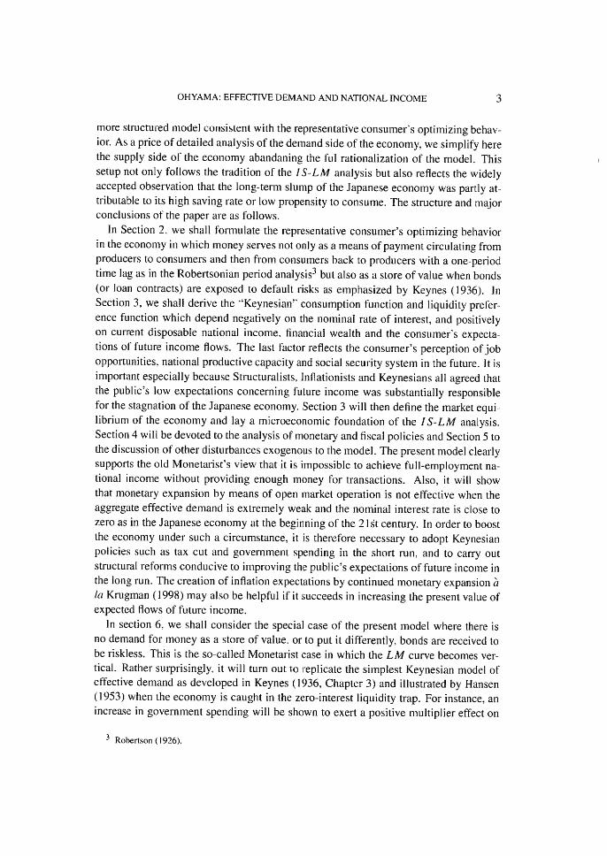
(2000) committing to a given target volume of money supply. The left-hand side of the above equation system contains two endogenous variables, it and Yt, whereas the right-hand side contains exogenous variables only. Without explicitly solving the system, one can show that there is a unique economically meaningful pair of equilibrium interest rate and national income when money supply is sufficiently large. Consider Figure 1 that displays a version of the familiar IS-LM diagram on the assumption that Mt/pr > h+ Gt. The downward sloping I S curve depicts the combination of it and Yr that satisfies equation (22). It is part of a rectangular hyperbola with horizontal asymptote passing through point (-1, 0) and vertical asymptote passing through point (0, It + Gt).The upward sloping LM curve shows the combination of it and Yt that satisfies equation

(23). It is part of a quadratic curve along which Yt converges to Mt/pt as it tends to infinity. Clearly, there is only one intersection of the IS and LM curves where it and Yt are positive and Yr is greater than It + G, and smaller than Mr/ Pr •

PROPOSITION l . Given the private autonomous investment, the government expen-diture and money supply such that Mt/pt > It + Gt, there exists a unique meaningful equilibrium where the national income and interest rate are adjusted to clear both prod-uct and money markets.

Having confirmed the unique existence of the IS-LM equilibrium, we now turn to some comparative statics of the system.

4. FISCAL AND MONETARY POLICIES

Figure 1 makes it clear that the equilibrium value of Yr is trapped between I, +G, and

Mt/pt. On the one hand, there would be no product left for consumption if Yr < I, +G r . On the other hand, there would not be enough money for hoarding and transactions

13 For example, Romer (2000) proposes with good reasons these alternative versions of the 1 S-LM model.


1

IS LW r

E

/

/

^

i

E,

a e_0 •0

I, +G, YKi A/p Mill', YFr Y

Figure 1. The I S-LM Equilibrium and Monetary Expansion.

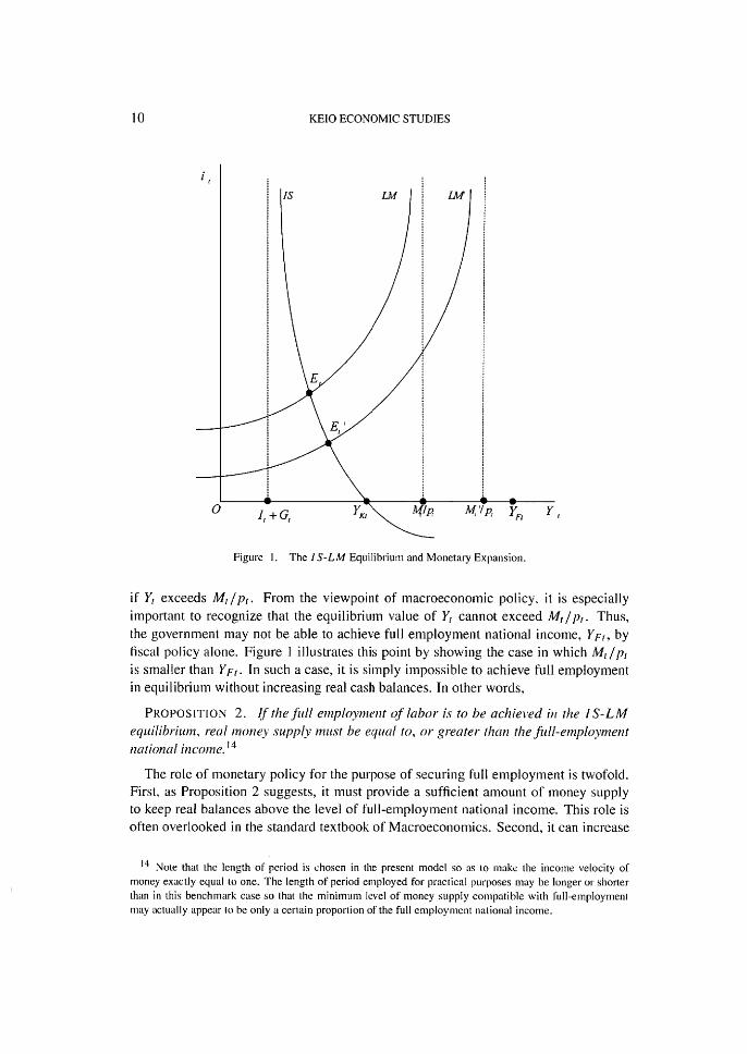
if Y, exceeds M,/p,. From the viewpoint of macroeconomic policy. it is especially important to recognize that the equilibrium value of Y, cannot exceed Ml/pt. Thus, the government may not be able to achieve full employment national income, Ypt, by fiscal policy alone. Figure 1 illustrates this point by showing the case in which M,/p, is smaller than YF,. In such a case, it is simply impossible to achieve full employment in equilibrium without increasing real cash balances. In other words,

PROPOSITION 2. If the full employment of labor is to be achieved in the 1 S-LM equilibrium, real money supply must be equal to, or greater than the full-employment national income. l ̀l

The role of monetary policy for the purpose of securing full employment is twofold.

First, as Proposition 2 suggests, it must provide a sufficient amount of money supply to keep real balances above the level of full-employment national income. This role is

often overlooked in the standard textbook of Macroeconomics. Second, it can increase

t4 Note that the length of period is chosen in the present model so as to make the income velocity of

money exactly equal to one. The length of period employed for practical purposes may be longer or shorter

than in this benchmark case so that the minimum level of money supply compatible with full-employment

may actually appear to be only a certain proportion of the full employment national income.


national income and employment by increasing money supply when national income is less than the full employment level. In fact, an increase in money supply by means of open-market purchasing of government bonds does not affect the IS curve but shifts the LM curve rightward bringing about a fall in interest rate and a rise in national income. This analysis of monetary policy is only familiar to any student of Macroeconomics. Regarding this second role, however, the present model also reveals the important but often ignored point that monetary policy of this type alone may not be capable of achiev-ing full employment when the level of aggregate demand is extremely low. To see this

point, note that no one would be willing to lend money if the nominal rate of interest were negative. Therefore, the equilibrium value of nominal interest rate cannot be neg-ative. Denote by YKt the effective demand for national product when the nominal rate of interest is zero. It is given by setting it = 0 in (22) as

($— Y)YKt = (1 +i8— y)it + (f — Y)Gr+(l + 7t)Zr+I +Vt . (24) Pt

Now, YKt may be smaller than YF•t in deep depression where the determinants of ag-

gregate demand in the right-hand side of (24) are very weak. Figure 1 depicts such a situation. Note that the central bank's open market operation does not affect the value of the consumer's financial asset, Mt + Ht. Thus it cannot increase the national income beyond YKt and hence cannot achieve the full employment if YKt < YFt•

PROPOSITION 3. Monetary expansion by means of open market operation lowers the rate of interest and thereby increases the national income. It is, however, incapable of achieving full-employment income in deep depression where YKt < YFt•

It is certainly possible, however, to achieve full-employment income even under such a circumstance, by printing money and giving it to the public as income subsidy (the so-called helicopter-money injection). This method of monetary expansion is effective since it increases Vt, or Mt + Hl. It can be regarded as a combination of monetary

policy (money printing) with fiscal policy (tax cut) to which we now turn. Let us consider the effect of a fiscal expansion when money supply is insufficiently

provided. By assumption, the present model only allows for balanced budget expansion to secure full employment. The usual textbook presumption is that the associated fiscal multiplier is less than unity since the balanced budget multiplier would be unity only when the rate of interest were unchanged but it actually rises as a result of the fiscal expansion. In the present model, the balanced budget multiplier should also be less than unity, but greater than the size of usual presumption. The inspection of (22) and (23) immediately reveals that the /S curve shifts rightward exactly by the size of the increase in the government expenditure and the LM also shifts rightward by less than the shift of the I S curve. Figure 2 shows this case where it shifts the L M curve concomitantly in the rightward direction to dampen the rise in the interest rate and alleviating its crowding-out effect.

PROPOSITION 4. Suppose that the consumer has a positive liquidity preference, i.e., y > 0. A tax-financed increase in the government expenditure raises interest rate


Figure 2. Fiscal Expansion.

and increases the national income. The associated fiscal multiplier is less than one but greater than the magnitude implied in the standard textbook where the LM curve remains unaffected in the face of balanced-budget fiscal expansion.

The rate of increase in national income will decrease, however, as the government expenditure increases. A concomitant sharp rise in the rate of interest will crowd out

consumption expenditure to offset the increase in the government expenditure as na-tional income approaches the available amount of real cash balances. The effect of autonomous investment on national income is presumably greater than that of fiscal ex-

pansion of the same size because the former shifts the I S curve much more than the latter although it leaves the LM curve unaffected.


5. KNIGHTlAN UNCERTAINTIES AND OTHER DISTURBANCES

At this point, we wish to draw the reader's attention to two distinct sources of Knigh-tian uncertainty latent in the present model economy. One is uncertainty about future

earnings. The consumer is supposed to estimate the exact value of her future non-interest incomes but may not feel certain about her estimation. For instance, she may have static expectations with respect to future earnings but feel uncertain about them.

This kind of Knightian uncertainty is likely to affect her utility function. We assume that her discount rate of expected future incomes rises to decrease the discounted value of her expected future incomes, Zr+i, when her sense of uncertainty gets stronger.15

This decreases her disposable wealth WI thereby shifting /S curve left ward and the LM curve rightward. The inspection of (22) and (23) immediately reveals, however,

that the the shift of the IS curve is larger than that of the LM if is not too am all and

y is not too large.16

PROPOSITION 5. Suppose that the consumer has a positive liquidity preference.

i.e., y > 0. An increase in the uncertainty of future earnings will lower the interest rate and decrease the national income under normal circumstances.

Clearly, a rise in the the present value of the future earnings, (1 + ht)Zr+I, increases the disposable wealth and exerts positive effects on the national income.17 These com-

parative statical results may be taken to endorse some policy proposals for combating structural depression due to deficient aggregate demand. For instance, some argue for creating expectations for inflation (e.g., Krugman (1998)) and others for carrying out reforms in government public enterprises (e.g., the Koizumi cabinet of Japan at the be-

ginning of the 21st century-) as possible remedies for the decade-long depression in the Japanese economy. In view of the present model, these proposals are meaningful as long

as they are capable of increasing the consumer's expected future earnings, (1 +tr)Z,+1, in one way or another.

Another source of uncertainty is the possible default of loan contract, which gives rise to liquidity preference. The consumer is supposed to possess no knowledge of objective

probability distribution of default but perceive uncertainty of loan contract and translate it into her liquidity preference. The intensity of liquidity preference is here summarily indicated by parameter y. An increase in perceived uncertainty of loan contract, or a rise in y, increases speculative demand for money and at the same time decreases the

propensity to save. Thus it shifts the LM curve left ward and the IS curve rightward concomitantly. The inspection of (22) and (23) reveals that the shift of the IS curve is

15 See Appendix for an explanation . 16 The exact condition for this result is given by

(I +it)y+j +(l +it)/3)lit

We may assume that this condition is satisfied under normal circumstances. 17 See Appendix for an explanation .


normally smaller than that of the LM curve.18

PROPOSITION 6. Suppose that the consumer has a positive liquidity preference,

i.e., y > 0. An increase in her liquidity preference will raise the interest rate and decrease the national income under normal circumstances.

The confidence in the loan contract is thus an important factor in the determination of business conditions. The ill-performing banking system has aggravated the depression in Japan partly because it has weakened the public's confidence in the loan contract. The central bank must increase money supply to compensate for a decline in the confidence if it is to maintain the equilibrium national income.

The consumer's propensity save, as determined by 16 — y, reflects her evaluation of the future consumtion relative to the present consumtion. A rise in f3 shifts the IS curve left ward and the LM curve rightward.

PROPOSITION 7. Suppose that the consumer has a positive liquidity preference, i.e.. y > 0. Given y, an increase in her propensity, to save will lower the interest rate and decrease the national income when liquidity preference measured by y is weak. Its effect on the national income may, be reversed when liquidity, prefer-ence is extremely strong.

The propensity to save is likely to increase if the prospect of publicly financed con-sumption (e.g., through the social security system) deteriorates as is the case with the

present-day Japan. In fact, some of the Structuralist's reform proposals on the national medical and pension systems reduce the net income of the older generations and may

generate adverse effects on the aggregate effective demand. They must, therefore, be supplemented with compensating measures to reform the retirement system and pub-lic enterprises, which improve the expectations of the representative consumer's future earnings.

6. THE MONETARIST AND KEYNESIAN SPECIAL CASES

In this section, we consider the Monetarist special case when there is no liquidity

preference, or y = 0.19 We will argue that the Keynes—Ilanses special case (as pre-sented in Chapter 3 of Keynes (1936) and later popularized ny Hansen (1953)) may be

conceived as a special case of this Monetarist model where aggregate effective demand is extremely low because of high propensity to save and weak expectations concerning

future earnings. This interpretation is unorthodox at least in two respects. First, the Keynes—Hansen special case is usually considered to arise when the IS schedule be-

comes vertical because of inelasticity of demand with respect to interest rate. Second,

18 A sufficient condition for this result is

(I — >2y+------ I + i2

which can be satisfied when y is small compared with ll. 19 The Monetarist special case is said to arise when the LA1 curve becomes vertical . For instance. see

Tobin (1974).

OHYAMA: EIH't-"hCTIVE DEMAND AND NATIONAL INCOME 15

the Keynes-Hansen special case is usually contrasted with the Monetarist special case as if they are the two polar cases of the general I S-LM model. The present interpreta-tion neither rests on the interest-inelasticity of aggregate demand. nor does it separate the Keynes—Hansen case from the Monetarist case in the orthodox fashion.

With y = 0, (23) reduces to the simple quantity equation of money:

Mt(25) Yr= —. P

t which gives the equilibrium value of Yt corresponding to the given value of M,/p,. The vertical LM line in Figure 3 shows the graph of this equation. As Monetarists argued, money supply appears to be the sole factor in the determination of equilibrium national income in this special case. The demand for national product coming from

private investment and government expenditure plays no role there. The downward-sloping IS curve depicts the combination of it and Y, that satisfies (22). It determines the equilibrium interest rate, given the value of financial wealth lit/pt. Substituting (25) into (22) and rearranging terms, we get

1 + it _Ir+ (1 + ht )Z,+l-l-vt/Pt(26) )3( t/Pt — GI - It)

where Mt/pt —GI— 1, > 0. An increase in money supply increases the equilibrium national income and lowers the equilibrium interest rate as long as Ml/p, < YFt. In contrast, an increase in government expenditure, or in any other exogenous expenditure, fails to affect the equilibrium income. It merely brings about a rise in the equilibrium interest rate. The crucial assumption here is the absence of liquidity preference. Clearly, It leads to the well-known Monetarist proposition that there can be no change in equi-librium income without a corresponding change in money supply.20

In view of (26), the nominal rate of interest is non-negative if

MrHt (,8-1)—<(1+fl)Ir+l8Gt+(1+7t)Zr+1+—. (27)

PtPr The right-hand side of inequality (27) is positive. Clearly, this inequality is satisfied if 8<1.

PROPOSITION 8. If the consumer has no liquidity preference (i.e., y = 0), the Monetarist special case obtains under condition (27).

This proposition clarifies the role of liquidity preference in the I S-L M analysis. The existence of liquidity preference is indispensable for the efficacy of fiscal policy per se. In fact, in the absence of liquidity preference, an increase in any component of effective demand such as government expenditure and investment cannot increase the equilibrium national income by itself without the help of accommodating increase in money supply.

20 The original Monetarist interpretation of the IS -LM model was given by Friedman (1970 , 1971). See Tobin (1974) for some critical comments.


it

~rt

0

Is IM

N

•

I, • +•G,Mp, 'Fr~°

Figure 3. The Monetarist Special Case.

The monetary authority can increase money supply without precipitating monetary disequilibrium only up to the critical value given by the right hand side of inequality (27). Once the critical value is reached and the corresponding equilibrium interest rate falls to zero, the monetary authority must take it as given and adjust money supply so as to maintain equilibrium in the commodity and money markets. To use the terminology of Romer (2000), the switch from a money supply rule to an interst rate rule is bound to take place at this point. Under the present setup, this state of the economy may be identified with the Keynesian "liquidity trap" in the sense that the nominal interest rate cannot fall any further.Ll We reproduce (24) obtained by setting it = 0 in (22) in a slightly different form:

21 Usually, "liquidity trap" is defined as the state in which liquidity preference becomes absolute after the

rate of interest has fallen to a very low level. See Keynes (1936, p. 207) and Friedman (1974, p. 24). The

present special case differs from such a state since the consumeris assumed to possess no liquidity preference. The liquidity trap in the usual sense could arise in the present model when the consumer has a liquidity

preference (i.e., y > 0) and the rate of interest falls to zero. Note, however, that such a state would never be realized in equilibrium.


1 + /3 IVr Yxr = Ir + Gr -I- (1 -I- irr)Zr+t +

Pr. (28) One can easily see that the investment multiplier is given by (1 ,8)/if3 and that the balanced budget multiplier is equal to unity. The real financial wealth , expected rate of inflation and expected real value of earnings in the future positively affect the equilib-

rium income. Their multiplier is given by 1/fl and is smaller than unity . The central bank's open market operation does not affect YKr since it leaves vt unchanged at its

given historical value. If YKt is less than the full employment income YFr, this equilib-rium may be interpreted as the Keynesian special case where monetary policy becomes

powerless under the "liquidity trap" and the equilibrium national income is determined only by exogenously given government expenditure, private investment, real financial wealth and the expected real value of earnings together with the expected rate of infla-tion.

PROPOSITION 9. If the consumer has no liquidity preference (i.e., y = 0), the Keynes-Hansen special case arises when it = 0 and Yxr < YFr.

0

in 1

AL

IS L44

A -I, +G,11/1 , / 1),(=YKr I TY: FtY,

Figure 4. The Keynes—Hansen Special Case.


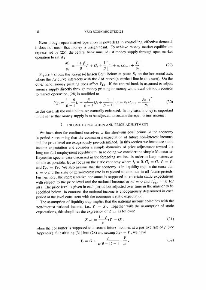
Even though open market operation is powerless in controlling effective demand, it does not mean that money is insignificant. To achieve money market equilibrium represented by (25), the central bank must adjust money supply through open market operation to satisfy

Mt I + ,BlVr — =-----It + G t +(1 + r,) Zt+i +. (29) Pt Figure 4 shows the Keynes—Hansen Equilibrium at point Et on the horizontal axis

where the IS curve intersects with the LM curve (a vertical line in this case). On the other hand, money printing does affect YKt. If the central bank is assumed to adjust smoney supply directly through money printing or money withdrawal without recource to market operartion, (28) is modified to

1At—i YKt _I +~3Ir+G,+1(1+ ;r,)Zt+1+p

t(30) 1 /3-

In this case, all the multipliers are naturally enhanced. In any case, money is important in the sense that money supply is to be adjusted to sustain the equilibrium income.

7. INCOME EXPECTATION AND PRICE ADJUSTMENT

We have thus far confined ourselves to the short-run equilibrium of the economy

in period t assuming that the consumer's expectation of future non-interest incomes and the price level are exogenously pie-determined. In this section we introduce static

income expectation and consider a simple dynamics of price adjustment toward the long-run full-employment equilibrium. In so doing we consider the simple Monetarist-

Keynesian special case discussed in the foregoing section. In order to keep matters as simple as possible, let us focus on the static economy where I, = 0, Gt = G, Vt = V,

and YF, = YF. We also assume that the economy is in liquidity trap in the sense that it = 0 and the state of zero-interest rate is expected to continue in all future periods. Furthermore, the representative consumer is supposed to entertain static expectations

with respect to the price level and the national income, or ht = 0 and Yr+,. = Yt for all t. The price level is given in each period but adjusted over time in the manner to be specified below. In contrast, the national income is endogenously determined in each period at the level consistent with the consumer's static expectation.

The assumption of liquidity trap implies that the national income coincides with the non-interest national income, i.e.. Yt = X,. Together with the assumption of static expectations, this simplifies the expression of Zt+i as follows:

Zr+1 =1-------7- p (Yt G) ,(31) P

when the consumer is supposed to discount future incomes at a positive rate of p (see Appendix). Substituting (31) into (28) and setting YKr = Ft, we have

Yr = G+ p •V,(32) p(,3— I)- 1 pt


PIr F Taking account of (32), we can rewrite (34) as

pt +1 = 1 — a 1 — YFpt(ap—1Y.,=(_Pr)(35)V P)E This is a linear difference equation of the price level with the stationary value:

pV i = ------------------------- l (YE — G)(P(8 —1)— 1) .(36)

Thus, condition (33) also guarantees the existence of the stationary eqquilibrium. Figure 5 illustrates the dynamics of the price adjustment, assuming

a l — — < 1 .(37)

This assumption is satisfied if the speed of adjustment is slow, e.g.. if a < 1. The process of price djustment monotonically leads to the stationary equilibrium, EL, in the long run where the full employment income is realized. Clearly, there can also be

provided that

P (18 — l) > 1 .(33)

PROPOSITION 10. Suppose that the economy is static and the Monetarist-Keynesian special case prevails. Condition (33) ensures the existence of market equi-librium under static income expectation. The equilibrium national income depends pos-itively on the government expenditure and the real .financial wealth, and negatively on the consumer's propensity to save and subjective discount rate of future incomes.

Note that the fiscal multiplier is unity as before, but the real financial wealth effect on the national income is considerably enhanced, compared with the case of exogenously

given income expectations. This is because the increase in the current income due to an increase in the real financial wealth gives rise to corresponding increases in expected future incomes. The contrast brings out the importance of how a change in the current income affects income expectations in future periods.

The price level is assumed to be given in each period, but suppose that it is ad-

justed upward (resp. downward) across periods when the current output is greater (resp. smaller) than the full-employment output. This adjustment process may be interpreted to reflect the underlying Walrasian adjustment of the wage rate in the labor market.22 To be specific, it is assumed to proceed according to

Pt+A — hr Yt — YF

iinis assumption is satisned ine speed et adjustment is slow, e.g., if a < 1. The process of price djustment monotonically leads to the stationary equilibrium, EL, in the long run where the full employment income is realized . Clearly, there can also be oscillatory or divergent solutions for (34) depending on the speed of adjustment.

PROPOSITION 11. Suppose that the economy is static and the Monetarist-Keynesian special case prevails with static income expectation. Suppose also that the

22 This follows the conventional assumption of price adjustment employed in the literature since Dorn-busch (1976).


P

P

Figure

p

5. Dynamics of Price Adjustment.

Pt

price level is adjusted according to the mechanism defined by (34). The long-run full-employment equilibrium exists if and only if the condition (33) is satisfied. Moreover, it

is globally stable if the speed of adjustment is sufficiently small, or

a < YF(38) YF — G

If this mechanism works, the Keynesian equilibrium will coincide with the classical full-employment equilibrium in the long run. It may take a very long time, however,

for this happy coincidence to be realized. The prolonged stagnation of the Japanese economy during lggo's extending into the 21 Century suggest that the mechanism could work but only slowly.

8. CONCLUDING REMARKS

The state of the Japanese

roughly approximated by the

economy at the beginning of the

Keynesian equilibrium described

21st century may be

in the preceding sec-


tion.23 In fact, the the Keynes—Hansen special case becomes relevant in the deep depres-sion where the people expect extremely low earnings in the future and their propensity to consume is also very weak. The model seems to shed some light to the diagnoses and remedies proposed by different camps of economists for the ailing Japanese econ-omy. The analysis of the model suggests that while the government's fiscal expansion is effective in increasing the equilibrium income unless it negatively affects the public's long-run expectations, the central bank must also increase money supply conformably to support the fiscal policy. Thus, money is important, but the monetary policy in the form of open market operation is powerless without fiscal expansion. It is also notewor-thy that the expected real value of earnings in the future, as well as the expected rate of inflation, affects the equilibrium income. Thus "structural reforms," improving the ex-

pected future income would unambiguously increase the equilibrium income. Raising the expected rate of inflation may also be helpful if it is feasible. It would be, however, extremely difficult to create inflation expectations and control the level of real balances appropriately under the assumed circumstances.

The limitations of the present analysis are more or less obvious. In order to avoid misunderstandings, however, let us mention some of them and consider the possibility of excuse or extension. First, the present formulation of the representative consumer's utility maximization assumes away the distinction between different individuals and different periods in the future. The abstraction from individual differences may be se-rious in some cases where redistributional or strategic relationships are important, but it can be justified as a first approximation when such relationships are unimportant at least in the analysis of the aggregate economy. The abstraction of periodical differences may be restrictive if one is interested in the entire profile of the consumer's life-time consumption, but it is tolerable in view of her bounded rationality when one wishes to explore her decision of how much to consume in the present period and how much to save for future periods. Second, the results of the paper rests on the simplifying but annoying assumption that the government refrains from borrowing and carries no out-standing debt. Undoubtedly, this assumption is unrealistic and dissatisfactory in view of the present Japanese economy conflicted with an enormous amount of national public debt. The relaxation of the assumption would, however, complicate the analysis consid-erably. Third, in order to illuminate the demand side of the economy, we deliberately simplified the supply side by assuming that the representative consumer (or worker) is willing to work up to certain hours at a given real wage and that firms are ready to pro-duce as much as demanded in the market. Moreover, money wage and the price level are assumed to be fixed in the short run. There are some well-known ideas to justify these assumptions24 but we have not attempted to incorporate them into the present model. Fourth, the treatment of investment in this paper is obviously restrictive, but it can be modified without much difficulty.

23 Many authors, notably Krugman (1998), argue that the Japanese economy has been stuck in the "liquid-

ity trap" for a long time. 24 See for instance

, Blanc hard and Fischer (1989), Chapter 9.


APPENDIX

As we discussed in the text, the representative consumer's long term expectation for future earnings (captured by Zt+i) is considered to affect her consumption decision. For instance, we may formulate Zt+1 as,

(1 +ht+l)(1 — pt+2)(Xet+Lc ~—T) Zt+1=(1—pt+1)(Xi+l—Trel)+tI2 +.. • 1 + It+1

where ps is the consumer's subjective discount rate of expected earning in period s and (_ (Ps — Ps-FT )/Ps)) is the expected rate of inflation from period s to period s + 1,

and Xi+s and Tr+s are the expected non-interest income and the expected tax in period t + s.The consumer niay lose her job permanently because of serious illness or sudden accident, or she may not be able to secure incomes as expected for some other reasons such as possible changes in social security provisions or in business climate in future periods. In the above formulation of Zt+l, ps may be interpreted to reflect this kind of Knightian uncertainty.

When the consumer's expectations are static, i.e., res = it, is = i, ps = p and Xs — Ts = X — T for s = t + 1, t + 2, .... the above formulation simplifies to

Zt+1 =(1 +i)(1 — P) (X — T) . P+i—(1 —P)Z

Thus, Zt+1 converges to a finite value even when the expected rate of nominal interest is zero. Clearly, it increases with the expected rate of future inflation and decreases with the subjective discount rate given the real value of non-interest income flow net of tax.The above expression can also be written

A where r is the real rate of interest defined by the Fisher relation:

i — :r r =-------

1 + 7r Thus. 4+1 takes on a positive finite value even when the real interest is negative as long as r + p > 0. An increases in the real rate of interest decreases Z,±1.

REFERENCES

Blanc hard, Oliver J. Macroeconomics, Upper Saddle River, NJ: Prentice-Hall, 1996. Blanc hard, Oliver J. and Fischer, Stanley. Lectures on Macroeconomics. Cambridge, MA: The MIT Press,

1989. Blanc hard, Oliver J. and Kiyotaki, Nobuhiro. "Monopolistic Competition and the Effects of Aggregate De-

mand." American Economic Review, 77(4), September 1987, pp. 647-666. Dornhusch, Rudigar. "Expctations and Exchange Rate Dynamics:' Journal of Political Economy, 84, De-

cember 1976, pp. 141-153. Friedman, Milton. "A Theoretical Framework of Monetary Analysis," in Milton Friedman's Monetary Frame-

work: Debate with His Critics. ed. Robert J. Gordon. Chicago: University of Chicago Press, 1974. Hansen, Alvin. H. A Guide to Keynes, New York: McGraw-Hill, 1953. Hicks, John Richard, "Mr. Keynes and Classics" Econometrica, 5(2), 1937, pp. 147-159.


Hicks, John Richard, Value and Capital, London: Oxford University Press. Keynes, Maynard J. The General Theory of Employment, Interest and Money, London: Macmillan and

Co.,1936. Krugman, Paul. "It's baaack! Japan's Slump and the Return of the Liquidity Trap," Brookings Paper on

Economic Activity, 2, 1998, pp. 137-187. McCallum, Bennet T. and Nelson, Edward. "An Optimizing IS-LM Specification for Monetary Policy and

Business Cycle Analysis." Journal of Money, Banking and Credit, 31, 1999, pp. 296-316. Mankiw, N. Gregory, Macroeconomics. New York, NY: Worth Publishers, Inc. 1992_ Nealy, J. Peter and Stiglitz, Joseph E. "Toward a Reconstruction of Keynesian Economics: Expectations and

Constrained Equilibria," Quarterly Journal of Economics, 98, Supplement, 1983, pp, 199-228. Robertson, Dennis H. Banking Policy and the Price Level: An Essay in the Theory of the Trade Cycle, London:

P. S. King and Son Ltd., 1926. Siivestre, Joaquim. "The Market-Power Foundations of Macroeconomic Policy," Journal of Economic Liter-

ature, 31, March 1993, pp. 105-141. Tobin, James. "Friedman's Theoretical Framework," in Milton Friedman's Monetary Framework: Debate

with His Critics, ed. Robert J. Gordon. Chicago: University of Chicago Press, 1974.

title effective demand and national income : a

Documents