© 2015 IEEE. Personal use of this material is permitted. Permission from IEEE must be obtained

for all other uses, in any current or future media, including reprinting/republishing this material for

advertising or promotional purposes, creating new collective works, for resale or redistribution to

servers or lists, or reuse of any copyrighted component of this work in other works.

Title: Spectral and Spatial Classification of Hyperspectral Images Based on ICA and Reduced

Morphological Attribute Profiles

This paper appears in: IEEE Transactions on Geoscience and Remote Sensing

Date of Publication: 2015

Author(s): Nicola Falco, Jon Atli Benediktsson, Lorenzo Bruzzone

Volume: 53

Issue: 12

DOI: 10.1109/TGRS.2015.2436335

1

Spectral and Spatial Classification of

Hyperspectral Images Based on ICA and

Reduced Morphological Attribute ProfilesNicola Falco, Student Member, IEEE, Jon Atli Benediktsson, Fellow, IEEE,

and Lorenzo Bruzzone, Fellow, IEEE

Abstract

The availability of hyperspectral images with improved spectral and spatial resolutions, provides the opportunity

to obtain accurate land-cover classification. In this paper, a novel methodology that combines spectral and spatial

information for supervised hyperspectral image classification is proposed. A feature reduction strategy based on

Independent Component Analysis (ICA) is the main core of the spectral analysis, where the exploitation of prior

information coupled to the evaluation of the reconstruction error assures the identification of the best class-informative

sub-set of independent components. Reduced Attribute Profiles (rAPs), designed to address well known issues related

to information redundancy that affect the common morphological APs, are then employed for the modelling and

fusion of the contextual information. Four real hyperspectral data sets, characterized by different spectral and spatial

resolution with a variety of scene typologies (urban, agriculture areas), have been used for assessing the accuracy

and generalization capabilities of the proposed methodology. The obtained results demonstrate the classification

effectiveness of the proposed approach in all different scene typologies, with respect to other state-of-the-art techniques.

Index Terms

Supervised classification, dimensionality reduction, independent component analysis, mathematical morphology,

reduced attribute profiles, hyperspectral images, remote sensing.

I. INTRODUCTION

In the last few years, a new generation of hyperspectral sensors that are able to provide images with both high

spectral and high spatial resolution has been developed. Hyperspectral images are an increasingly important source

N. Falco is with the Faculty of Electrical and Computer Engineering, University of Iceland, 101 Reykjavik, Iceland (e-mail: nico-

lafalco@ieee.org).

J. A. Benediktsson is with the Faculty of Electrical and Computer Engineering, University of Iceland, 101 Reykjavik, Iceland (e-mail:

benedikt@hi.is).

L. Bruzzone are with the Department of Information Engineering and Computer Science, University of Trento, 38050 Trento, Italy (e-mails:

lorenzo.bruzzone@ing.unitn.it).

2

of information that has found use in a wide range of fields, from Earth observation (EO) to the assessment for food

quality, to the medical domain. Focusing on the EO field, and in particular on land-cover analysis, the burst of

informative content conveyed in hyperspectral images, represented by both high spectral and the spatial resolutions,

provides the base for obtaining high accuracy in the identification and classification of different land-covers of an

observed area of interest. These characteristics enforce the need of strategies that integrate the analysis of both

spectral and contextual domains in order to maximise the exploitation of the information combined in these images.

As expected, the processing of hyperspectral data is far from being straightforward, due to innate issues.

Considering the spectral domain, each single pixel is considered as an independent entity of information. The

high dimensionality makes the analysis computationally expensive, while the Hughes phenomenon (curse of di-

mensionality) [1] arises when the ratio between the number of available training samples and the number of

spectral channels is small. This affects the generalization capability of the classifier. Most studies in the current

literature address the curse of dimensionality issue by exploiting feature extraction / selection techniques, aiming

at decreasing the dimensionality of the feature space by retaining the most useful information. Based on the task

to be accomplished, i.e., compression, target detection, identification of endmembers and classification, several

feature extraction techniques have been developed, ranging from unsupervised to supervised approaches. The most

widely used unsupervised approaches include Principal Component Analysis (PCA) [2], [3] and Singular Value

Decomposition (SVD) [4], which provide an optimal representation in terms of least square error. Maximum Noise

fraction (MNF) [5] and Noise-Adjusted Principal Component (NAPC) [6] aim at identifying the projection that

maximises the signal to noise ratio, whereas Independent Component Analysis (ICA) [7] aims at identifying a linear

transformation that minimises the statistical dependence between its components. Supervised approaches, which

exploit prior information to extract class-discriminant features, include Discriminant Analysis Feature Extraction

(DAFE) [2], Decision Boundaries Feature Extraction (DBFE) [8], projection pursuit (PP) [9] and Non-Parametric

Weighted Feature Extraction (NWFE) [10]. All the aforementioned approaches are used in both pre- and post-

processing phase in order to overcome the high dimensionality issue in the classification task. Feature selection

techniques, which have the goal to select the most adequate sub-set of features without decreasing the information

content, have been widely used in remote sensing. The selection of a sub-set is usually based on the evaluation of

a fitness function followed by a search strategy. A number of statistical distance measures [2], such as divergence,

Bhattacharyya distance, Jeffries-Matusita (JM) distance and mutual information, are used to assess the separability

and / or the mutual dependency among class distributions based on the available training set. Sub-optimal strategies,

such as the Sequential Backward Selection (SBS) [11] and the Sequential Forward Selection (SFS) [12] methods,

are broadly used. More effective sequential search methods, the Sequential Forward Floating Selection (SFFS) and

the Sequential Backward Floating Selection (SBFS) methods [13] were proposed in order to avoid the nesting effect

that affects both SBS and SFS techniques by including and excluding features. The steepest ascent and the fast

constrained [14] algorithms are effective strategies that have shown better results compared to SFFS technique,

even if the required computation time is slightly higher. Furthermore, heuristic search algorithms based on the

evolutionary concept of natural selection, such as Genetic Algorithms (GAs) [15], have been widely employed in

3

several fields as well as in remote sensing.

When images with high spatial resolution are considered, the analysis of spectral information only is less effective.

In fact, on one hand, the improved spatial resolution makes different objects more distinguishable on the ground.

On the other hand, however, it increases the intraclass variability [16], leading to poor classification performances.

In order to minimise the uncertainty of the classification, the information related to the spatial context needs to be

included in the analysis. Recently, several methods developed as part of the mathematical morphology framework

have been proposed in retrieving and modelling contextual information also, both for remote sensing (RS) images

and other image types. Attribute profiles (APs) [17] have been successfully exploited in the RS domain to include

the spatial information in the analysis for different tasks, such as land-cover classification [18]–[20], segmentation

[21] and change detection [22]. APs provide a multi-level decomposition of the original image, which is obtained

by applying a more severe thinning/thickening filtering [23] on connected regions. APs are an interesting tool

as they extract contextual information performed according to specific attributes, i.e., measurements that can be

performed on a connected region. APs have many advantages: a) Different attributes can be defined, providing a

variety of different image decompositions; b) Attributes can be a measurement that is not related to the geometry

of the region (e.g., standard deviation); c) The filtering is performed on connected regions, while the geometrical

detail of the unfiltered regions is fully preserved. This high flexibility renders the APs a powerful tool for extracting

complementary spatial information of the structures in the scene. Because the APs are based on attribute filters

[23], which are binary operators, the extraction of contextual information based on attribute profiles is not trivial

when multi-channel images, such as hyperspetral data, are considered. The application of the attribute filters to

each spectral band would increase excessively the dimension of the final feature space, making the direct profile

extraction not feasible. In the literature, this issue is generally addressed by applying dimensionality reduction prior

to the filtering. That generates a vector of filtered images, named extended attribute profiles (EAPs) [18], which

consists of concatenated APs obtained by each feature. A further extension is obtained when several EAPs obtained

by different attributes are concatenated, obtaining the so-called extended multi-attribute profiles (EMAPs) [18].

This extension can effectively model the spatial information extracted by employing several attributes, providing

a rich description of the scene. As a consequence, when the dimensionality increases, the redundant information

contained in the profile increases also. This is evident if we examine the sparsity that characterizes the Differential

Attribute Profile (DAP) [17], which expresses the residual between two adjacent levels in an AP. Moreover, when a

large range of filtering thresholds is considered, the dimension of the feature space of the obtained profile increases

resulting in a very large number of features and, thus, in the Hughes phenomenon. In the literature, the issue was

investigated by considering many approaches. In [24], the high dimensionality was reduced by exploiting feature

extraction and feature selection techniques prior to classification, which is a strategy that has also been widely

exploited in recent studies [19], [20], [25]. A compact representation of the morphological profiles (MP), called

morphological characteristic (MC), was obtained in [21] by analysing the differential MP (DMP) to identify if the

underlying region of each pixel is darker or brighter than its surroundings. In [26], an extension of the MC was

presented, where the characteristics of scale, saliency, and level of the DMP are identified by a 3-D index for each

4

pixel in the image. A strategy based on a sparse classifier and SUnSAL (Sparse Unmixing by variable Splitting

and Augmented Lagrangian) [27] for the analysis of the entire EMAP, was presented in [28].

In this study, the previous works presented in [29], [30] are extended, proposing a novel approach to supervised

classification based on both spectral and spatial analysis. Considering the most recent studies, where APs are

exploited, the spectral analysis is usually relegated to the identification of few PCA components, which are then

exploited for building the APs, EAPs and EMAPs, while supervised feature extraction techniques (e.g., DBFE,

NWFE) are eventually employed in order to reduce the dimensionality of such huge vectors. In this study, the spectral

analysis becomes a fundamental part, which aims at extracting the optimal sub-set of class-informative features. To

this purpose, a feature reduction technique based on ICA is considered, where the selection of the most representative

components is assured by the minimisation of the reconstruction error computed on the training samples employed

for the supervised classification. The spatial analysis is then performed by extracting spatial features based on

mathematical morphology. A compact optimised representation of the AP, named reduced AP (rAP), is obtained by

evaluating the contextual information for each region by identifying the best level of representation, according to a

homogeneous measure. Such analysis permits the contextual information to be preserved and at the same time to

address the dimensionality issue, which leads to a highly intrinsic information redundancy, that affects the original

AP.

The paper is organized as follows. The theoretical background on ICA and mathematical morphology is presented

in Section II. In Section III the proposed spectral and spatial analysis for classification is described. The experimental

setup is given in Section IV, while the experimental results are discussed in Section V. Conclusions and future

steps are drawn in Section VI.

II. THEORETICAL BACKGROUND

In this section, we provide an introduction to the theoretical background on ICA and mathematical morphology,

needed for a better understanding of the presented work. Here, the mathematical notation of vectors and matrices are

denoted as bold lowercase and bold uppercase letters, respectively, where the elements of a matrix are considered

as column vectors. According to the notation, m

i

represents the i-th column of a matrix M, m

T

i

represents the i-th

row of M, and mj

is the element placed in the j-th position of the column vector m

i

.

A. Independent Component Analysis

1) General concept: ICA is a well-know technique used in blind source separation, which is the decomposition

of an observed set of mixture signals into a set of statistically independent sources or components. Let us consider

the observed mixture data X = [x1, ..., x

m

]

T , which can be defined as a linear combination of n random vectors

represented by S = [x1, ..., x

n

]

T , the linear mixing model can be defined as:

X = AS, (1)

where A represents the unknown mixing matrix with elements [a1, ..., a

n

]. Assuming that the mixing matrix A

is squared (m = n), the best approximation, Y, of the unknown source matrix, S, is obtained by estimating the

5

unmixing matrix W ' A

�1, which is used to compute the decomposition. The source matrix is then obtained by

applying the ICA model as follows:

Y = WX ' S, (2)

where Y represents the matrix of statistically independent components (ICs). In the RS literature, many ICA

algorithms based on the maximisation of different criteria can be found, such as FastICA [31], JADE [32] and

Infomax [33].

2) FastICA Algorithm: In this study, the FastICA algorithm is exploited for the ICA decomposition. FastICA is

based on the fixed-point iteration algorithm, where the negentropy, J , which is a measurement of non-Gaussianity,

is the function to be maximised. Negentropy is always positive, except for the Gaussian distribution case, where

its value is zero. Negentropy is defined as follows:

J(y) = H(y

Gaussian

)�H(y) (3)

with y being a random vector, H(y) the entropy of y and H(y

Gaussian

) the entropy of a Gaussian random vector

whose covariance matrix is equal to the one of y. Because of the high computational complexity of the negentropy,

a moment-based approximation was introduced [34]:

J(y) / [E{(G(y)}� E{G(v)}]

2 (4)

where y is a standardized non-Gaussian variable, v is a standardized Gaussian variable and G is a non-quadratic

function. The fixed-point iteration algorithm finds the maximum of the non-Gaussianity of w

T

x, where w represents

one row of W. The convergence is reached when the w and its update, obtained in the successive iteration, w

i+1,

point in the same direction. In this work, the FastICA c� package (version 2.5, 2005) has been used, choosing a

symmetric orthogonalization. This choice has the advantages to avoid the cumulative error in the estimation process

and allows the parallel estimation of the components, decreasing the computational time of the algorithm. The

readers are referred to [34] for a complete explanation of the algorithm.

B. Morphological Operators

Mathematical Morphology (MM) is a well-established framework built upon set theory, lattice algebra and integral

geometry, whose operators are exploited for the investigation of spatial features (i.e., geometry, shape, edges) of

geometrical structures present in an image [35]. Many are the operators, developed in literature and most of them

are defined for binary and grey-scale images. Dilation and erosion are the basic morphological operators. They

are based on a moving window (or kernel), called structuring element (SE). Let us consider an object in the

image as a connected region, which is a flat area where the pixels have the same value. In general, dilation causes

objects to dilate or grow in size, whereas erosion causes objects to shrink. The effect of the filtering, i.e., the way

objects dilate or shrink, depend upon the choice of the SE (shape and size). By combining dilation and erosion

we obtain the closing and opening operators. Those operators are used to remove objects that cannot contain the

SE, while preserving objects with a similar shape as the SE. However, a distortion of these objects that remain

6

after the filtering is introduced, with a consequent loss of information related to the geometrical characteristics of

the objects. This issue was solved by the introduction of closing and opening by reconstruction, which are based

on geodesic transformations and permit the preservation of the geometrical characteristics of the objects that are

not removed. A further advancement was made by the introduction of Morphological Profiles (MP), which is a

stack of filtered images obtained by a sequential application of a morphological filter by reconstruction with the

SE increasing in size at each step. In general, a single application of a morphological operator is not enough for

representing all the objects within the scene. The MP provides a multi-scale decomposition of the image, which

goal is to obtain a better representation of the scene by taking into account that objects can appear at different

scale. The reader is referred to [35], [36] for a complete background on morphological operators, and to [21] for

the definition of MP. All the aforementioned operators are based on the use of a SE, making the filtering highly

dependent on the shape of the used SE. A different approach was introduced in [23] with attribute filters, where the

morphological transformation is attribute-based, removing the constraint of choosing a particular shape of the SE.

Consequently, the effect of the filtering is not shape-dependent any more, whereas, it is adaptive to the considered

region and its surrounding. In a similar ways as for the morphological filters, it is possible for the attribute filters

to build a multi-scale representation of the images, i.e., morphological Attribute Profiles (APs) [17]. The APs are

the starting point of this study, and, thus, a more formal definition is given.

1) Morphological Attribute Filters: Morphological attribute filters are defined by morphological attribute opening

and morphological attribute closing operators [23]. Let I be a digital grey-scale image and Zn (n = 2, i.e., 2D

images) its definition domain. A morphological transformation, , is a mapping from a sub-set, E, of the image

domain, I , to the same definition domain, E, with (I) ! Zn. Considering a criterion T , the morphological

attribute opening on a binary image is defined as the union of two binary operators: binary connected opening,

(�

x

), which transforms the image I preserving only the connected region that contain a selected pixel x, and binary

trivial opening, (�

T

), which preserves or removes the connected region based on the evaluation of the criterion T .

The binary attribute opening is extended to the grey-scale case by applying a threshold decomposition [21] on I

at each of its gray level k, assigning at each pixel the maximum gray level achieved by the binary opening. The

morphological attribute opening can be formally defined as:

�T

(I)(x) = max

(k : x 2

[

x2Th

k

(I)

�

T

[�

x

(Thk

)]

), (5)

where Thk

(I) represents the binary image obtained by thresholding I at level k. By duality, morphological attribute

closing is defined as:

�T

(I)(x) = max

(k : x 2

[

x2Th

k

(I)

�

T

[�

x

(Thk

)]

). (6)

2) Morphological Attribute Profiles: Let us consider a family of increasing criteria T = {T�

: � = 0, ..., L},

with T0 = true 8C ✓ E, where � is a set of reference scalar values used in the filtering and C is a connected

region in the image. A morphological profile is obtained by applying a sequential filtering, where the criterion T�

is evaluated at each filter step. Following this definition, the attribute opening profile, ⇧

�

T , and the attribute closing

7

profile, ⇧

�

T , are defined as follows:

⇧

�

T (I) =

(⇧

�

T

�

: ⇧

�

T

�

= �T

�

(I), 8� 2 [0, ..., L]

), (7)

⇧

�

T (I) =

(⇧

�

T

�

: ⇧

�

T

�

= �T

�

(I), 8� 2 [0, ..., L]

), (8)

where �T� and �T� represent a morphological attribute closing and attribute opening, respectively. The attribute

profile, ⇧(I), is obtained by concatenating the opening and closing profiles as follows:

⇧(I) =

(⇧

�

T (I), I, ⇧�

T (I)

), (9)

where I = ⇧

�

T0 = ⇧

�

T0 correspond to the original grey-scale. It can be seen that the profile results in a vector

of 2L + 1 images. Another important operator that is extensively used in this work is the so-called Differential

Attribute Profiles (DAP). It is obtained by computing the derivative of the AP, and it shows the residual of the

progressive filtering, i.e., the connected regions that have been filtered between two adjacent levels of the AP, and

their relative grey values. The DAP can be defined as follows:

�(I) =

��

�

T (I), ��

T (I)

. (10)

In this case, the obtained profile is represented by a vector of 2L images. When the property of increasingness is

not met, the definitions of opening and closing become more general, with �T

� and �T

� denoting the thickening

and the thinning profiles, respectively.

3) Extension to Multi-Channel and Multi-Attribute: Morphological operators are in general non-linear connected

transformations computed on an ordered set of values. This means that any of their extension to multivariate values is

an ill-posed problem. The usual strategy is to apply the operator to each channel separately and fuse or create a stack

of the obtained profiles. However, in the case of hyperspectral images, which feature space has high dimensionality,

this strategy becomes unattainable. In [37], a morphological operator was applied to a sub-space of the original

data obtained by using PCA, and only the first most informative principal components (PCs) were considered.

The concatenation of each obtained MPs defines a new structure called Extended Morphological Profile (EMP). In

general, after performing dimensionality reduction, the morphological analysis is applied to the r retained features

f . The same procedure can be adopted for the APs case [18], resulting in the definition of Extended Morphological

Attribute Profiles (EAP):

EAP (I) =

(⇧(f(I)1), ⇧(f(I)2), ..., ⇧(f(I)

r

)

). (11)

A further extension, which is based on the flexibility of the AP in considering any possible measure applicable to

a connected region as criterion, is the concatenation of the EAPs obtained by different attributes, which results in

the Extended Multi-Attribute Profile (EMAP) [18] and is defined as follows:

EMAP (I) =

(EAP (I)

a1 , EAP (I)

a2 , ..., EAP (I)

a

q

), (12)

8

Reconstruction error estimation

Extraction of l couple (ai ,yiT)

. . .

Optimum mixing matrix Aopt

ICA

Reconstruction error estimation

Extraction of l couple (ai ,yiT)

ICA

DAP computation

Identification of lm levels

AP computation

Reduced AP1

. . . DAP computation

Identification of lm levels

AP computation

Reduced APn

. . .

rth feature1st featurenth class1st class

Reduced EAP

Hyperspectral data

Supervisedclassification

Spectral analysis Spatial analysis

Optimized sub-set of IC features

Classification map

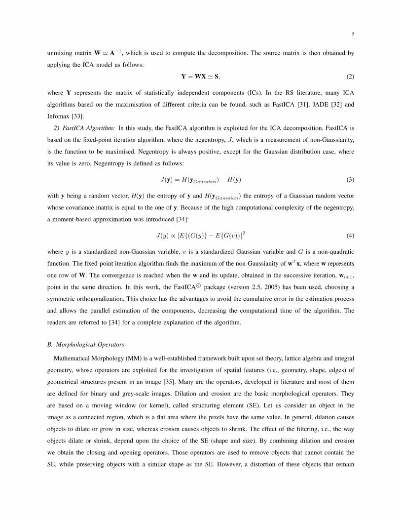
Fig. 1. General scheme of the proposed methodology for spectral and spatial classification.

where ai

represents the i-th given attribute, with i = 1, 2, ..., q. When the EMAP is built, a multiple presence of

the original PCs is included in the profile. This is avoided by including them once only in the first EAP and not

include them at all in the later EAPs.

III. PROPOSED METHODOLOGY FOR SPECTRAL AND SPATIAL CLASSIFICATION

The proposed methodology consists of two main parts: The first part is related to spectral analysis, where ICA

is exploited in order to retrieve class-informative features; the second part is related to contextual analysis, where

reduced APs are used to model the spatial information contained in the extracted ICs. The general scheme is shown

in Fig. 1.

A. Spectral Analysis: ICA-based approach for Dimensionality Reduction

The goal of the spectral analysis is to extract informative features that can be used in the classification task.

However, many studies have shown that not all the spectral space is needed for a good representation of the image.

On the contrary, a part of the spectral space contains information that is noisy and redundant. Feature reduction

techniques are usually adopted in order to extract a sub-space of informative features based on different criteria,

while discarding all the rest. Several studies [38]–[40] have demonstrated that when PCA is used prior to ICA for

dimensionality reduction, it provides a sub-set of components that does not preserve class-separability. This also

affects the independent components. The approach presented in this paper exploits the properties of ICA aiming at

extracting class-informative components for supervised classification purposes. ICA analysis is optimised to address

9

the supervised classification task based on the use of prior information provided by training samples. In [40], it

was shown that the reduction of the number of samples used as input to an ICA algorithm can in general improve

the ICA convergence speed, without affecting significantly the classification results. That was noticed in particular

in a low-dimensional scenario (i.e., dimensionality reduction was performed prior to ICA), whereas, when the

dimensionality reduction was not considered, the decrease of the number of training samples used as input to the

ICA was affecting negatively the performance of the classifier. In that case, the issue was to extract class-discriminant

features by exploiting only few samples in a high dimensional space. In the proposed approach, the ICA is applied

in a high-dimensional space (meaning that no dimensionality reduction is applied prior to ICA). This is due to the

fact that our aim is to find an optimised approach that effectively exploits the information extracted by ICA. The

ICA is separately applied to each class, extracting sets of ICs that are strictly dependent on the training samples

of each single class. The idea is to extract ICs specifically suitable to represent each specific class. After the ICA

decomposition, the reconstruction error is evaluated in order to identify the best ICs in terms of class representation.

The reconstruction error is, thus, exploited to address the issue related to the non-prioritization of the extracted ICs,

i.e., multiple applications of ICA provide different IC sets, which are diverse both in the order of appearance and

in content. The final sub-set is then optimised by applying a feature selection technique based on GA. Based on

our previous study [40], FastICA resulted the technique that provided the best performance in extracting the whole

source matrix, requiring less computational resources with respect to JADE and Infomax. Therefore, FastICA is

chosen here as the applied ICA decomposition technique. Let X be the observed data, represented by a m ⇥ p

matrix, with m spectral channels and p pixels, whose elements [x1, ..., x

m

]

T are the mixtures of the observed data.

Considering the model in (1), the linear mixing model adopted for hyperspectral images can be rewritten as:

X = AS =

mX

i=1

a

i

s

T

i

, (13)

where A is an m⇥m matrix and represents the unknown mixing matrix with elements [a1, ..., a

m

] and S is an m⇥p

matrix whose elements are the unknown sources [s1, ..., s

m

]

T . The proposed algorithm consists of the following

steps:

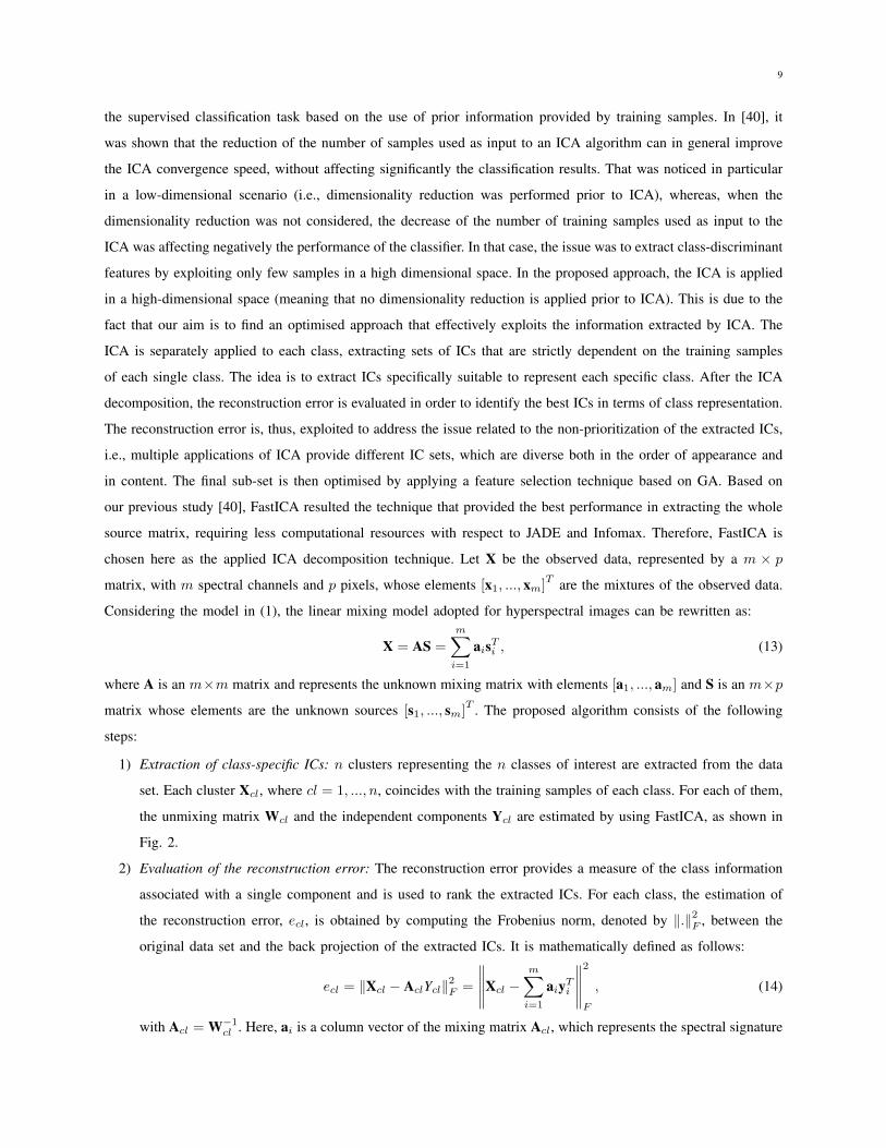
1) Extraction of class-specific ICs: n clusters representing the n classes of interest are extracted from the data

set. Each cluster X

cl

, where cl = 1, ..., n, coincides with the training samples of each class. For each of them,

the unmixing matrix W

cl

and the independent components Y

cl

are estimated by using FastICA, as shown in

Fig. 2.

2) Evaluation of the reconstruction error: The reconstruction error provides a measure of the class information

associated with a single component and is used to rank the extracted ICs. For each class, the estimation of

the reconstruction error, ecl

, is obtained by computing the Frobenius norm, denoted by k.k2F

, between the

original data set and the back projection of the extracted ICs. It is mathematically defined as follows:

ecl

= kXcl

� A

cl

Ycl

k2F

=

�����X

cl

�mX

i=1

a

i

y

T

i

�����

2

F

, (14)

with A

cl

= W

�1cl

. Here, a

i

is a column vector of the mixing matrix A

cl

, which represents the spectral signature

10

Yn

= Wn

Xn

Y1 = W1X1

Ycl

= Wcl

Xcl

Fig. 2. Clustering based on the training samples. A full size vector of ICs is extracted from each cluster separately.

No. features0 50 100 150 200 250

Error

ofreconstruction

×1011

0

0.5

1

1.5

2

2.5

3

3.5

4

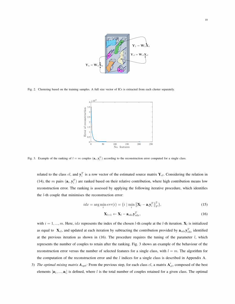
Fig. 3. Example of the ranking of l = m couples (ai

, y

T

i

) according to the reconstruction error computed for a single class.

related to the class cl, and y

T

i

is a row vector of the estimated source matrix Y

cl

. Considering the relation in

(14), the m pairs (a

i

, y

T

i

) are ranked based on their relative contribution, where high contribution means low

reconstruction error. The ranking is assessed by applying the following iterative procedure, which identifies

the l-th couple that minimises the reconstruction error:

idx = arg min

i

err(i) = {i | min

i

��X

l

� a

i

y

T

i

��2

F

}, (15)

X

l+1 X

l

� a

idx

y

T

idx

, (16)

with i = 1, ..., m. Here, idx represents the index of the chosen l-th couple at the l-th iteration. X

l

is initialized

as equal to X

cl

, and updated at each iteration by subtracting the contribution provided by a

idx

y

T

idx

identified

at the previous iteration as shown in (16). The procedure requires the tuning of the parameter l, which

represents the number of couples to retain after the ranking. Fig. 3 shows an example of the behaviour of the

reconstruction error versus the number of selected features for a single class, with l = m. The algorithm for

the computation of the reconstruction error and the l indices for a single class is described in Appendix A.

3) The optimal mixing matrix Aopt

: From the previous step, for each class cl, a matrix A

0cl

, composed of the best

elements [a1, ..., a

l

] is defined, where l is the total number of couples retained for a given class. The optimal

11

1 … 0 1 … 1 … 0 … 1

0 ... 1 1 … 0 … 1 … 0

1 … 1 0 … 0 … 0 … 1

class 1 class 2 class n

Aopt

=

�

��a1,1 · · · a1,l1 a1,1 · · · a1,l2 · · · a1,1 · · · a1,l

n

.

.

.

.

.

.

.

.

.

.

.

.

.

.

.

.

.

. · · ·.

.

.

.

.

.

.

.

.

am,1 · · · a

m,l1 am,1 · · · a

m,l2 · · · am,1 · · · a

m,l

n

�

��

chromosome

population

Aopt

=

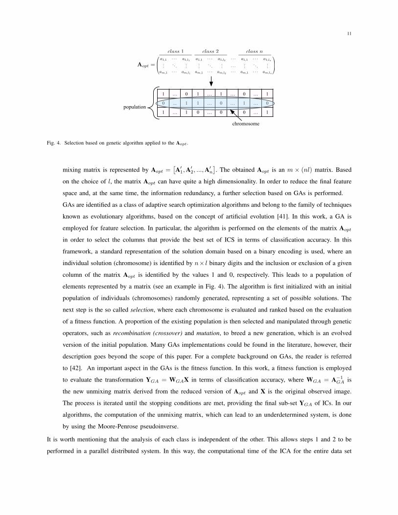
Fig. 4. Selection based on genetic algorithm applied to the A

opt

.

mixing matrix is represented by A

opt

=

⇥A

01, A

02, ..., A

0n

⇤. The obtained A

opt

is an m ⇥ (nl) matrix. Based

on the choice of l, the matrix A

opt

can have quite a high dimensionality. In order to reduce the final feature

space and, at the same time, the information redundancy, a further selection based on GAs is performed.

GAs are identified as a class of adaptive search optimization algorithms and belong to the family of techniques

known as evolutionary algorithms, based on the concept of artificial evolution [41]. In this work, a GA is

employed for feature selection. In particular, the algorithm is performed on the elements of the matrix A

opt

in order to select the columns that provide the best set of ICS in terms of classification accuracy. In this

framework, a standard representation of the solution domain based on a binary encoding is used, where an

individual solution (chromosome) is identified by n⇥ l binary digits and the inclusion or exclusion of a given

column of the matrix A

opt

is identified by the values 1 and 0, respectively. This leads to a population of

elements represented by a matrix (see an example in Fig. 4). The algorithm is first initialized with an initial

population of individuals (chromosomes) randomly generated, representing a set of possible solutions. The

next step is the so called selection, where each chromosome is evaluated and ranked based on the evaluation

of a fitness function. A proportion of the existing population is then selected and manipulated through genetic

operators, such as recombination (crossover) and mutation, to breed a new generation, which is an evolved

version of the initial population. Many GAs implementations could be found in the literature, however, their

description goes beyond the scope of this paper. For a complete background on GAs, the reader is referred

to [42]. An important aspect in the GAs is the fitness function. In this work, a fitness function is employed

to evaluate the transformation Y

GA

= W

GA

X in terms of classification accuracy, where W

GA

= A

�1GA

is

the new unmixing matrix derived from the reduced version of A

opt

and X is the original observed image.

The process is iterated until the stopping conditions are met, providing the final sub-set Y

GA

of ICs. In our

algorithms, the computation of the unmixing matrix, which can lead to an underdetermined system, is done

by using the Moore-Penrose pseudoinverse.

It is worth mentioning that the analysis of each class is independent of the other. This allows steps 1 and 2 to be

performed in a parallel distributed system. In this way, the computational time of the ICA for the entire data set

12

Mapping

Attribute Profile (AP)

Differential Attribute Profile (DAP)

Level Maps

Reduced Attribute Profile (rAP)

Thinning ProfileThickening Profile

a)b)

c)

d)

... .........

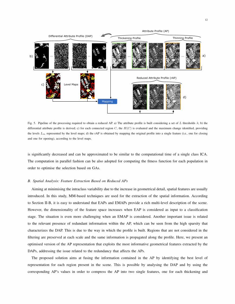
Fig. 5. Pipeline of the processing required to obtain a reduced AP. a) The attribute profile is built considering a set of L thresholds �; b) the

differential attribute profile is derived; c) for each connected region C, the H(C) is evaluated and the maximum change identified, providing

the levels Lm

represented by the level maps; d) the rAP is obtained by mapping the original profile into a single feature (i.e., one for closing

and one for opening), according to the level maps.

is significantly decreased and can be approximated to be similar to the computational time of a single class ICA.

The computation in parallel fashion can be also adopted for computing the fitness function for each population in

order to optimise the selection based on GAs.

B. Spatial Analysis: Feature Extraction Based on Reduced APs

Aiming at minimising the intraclass variability due to the increase in geometrical detail, spatial features are usually

introduced. In this study, MM-based techniques are used for the extraction of the spatial information. According

to Section II-B, it is easy to understand that EAPs and EMAPs provide a rich multi-level description of the scene.

However, the dimensionality of the feature space increases when EAP is considered as input to a classification

stage. The situation is even more challenging when an EMAP is considered. Another important issue is related

to the relevant presence of redundant information within the AP, which can be seen from the high sparsity that

characterizes the DAP. This is due to the way in which the profile is built. Regions that are not considered in the

filtering are preserved at each scale and the same information is propagated along the profile. Here, we present an

optimised version of the AP representation that exploits the most informative geometrical features extracted by the

DAPs, addressing the issue related to the redundancy that affects the APs.

The proposed solution aims at fusing the information contained in the AP by identifying the best level of

representation for each region present in the scene. This is possible by analysing the DAP and by using the

corresponding AP’s values in order to compress the AP into two single features, one for each thickening and

13

thinning profile. Since the reduced AP is directly extracted from the original AP, it has also the same limitations

when multi-channel data are considered. The extension to hyperspectral data analysis is obtained by applying the

morphological analysis to the sub-set of features identified by applying the proposed ICA-based feature reduction.

The following steps describe the methodology (Fig. 1) related to a single attribute case. The same procedure is

thus repeated for each attribute considered in the analysis. In Fig. 5 an example of the pipeline to obtain a single

reduced AP is shown. The steps are:

1) Computation of the AP and DAP: The first step is to build the AP. The critical phase in this part is the

choice of the � range values used as reference for the filtering phase. An optimal choice of the range values

is the one that provides a proper representation of the regions present in the scene. This is highly dependent

on the chosen attribute, and is usually based on prior information of the scene. The DAP is obtained by

differentiating the AP.

2) Region extraction: The DAP represents the residual of the AP, meaning that each level shows the regions that

have been filtered between two adjacent levels of the AP, in terms of grey-level values. This characteristic

allows the identification of connected regions related to each grey-value of the DAP with the advantage of

preserving the geometrical shape without any lost in terms of detail. From this step, thinning and thickening

profiles are analysed separately due to the different information that they provide.

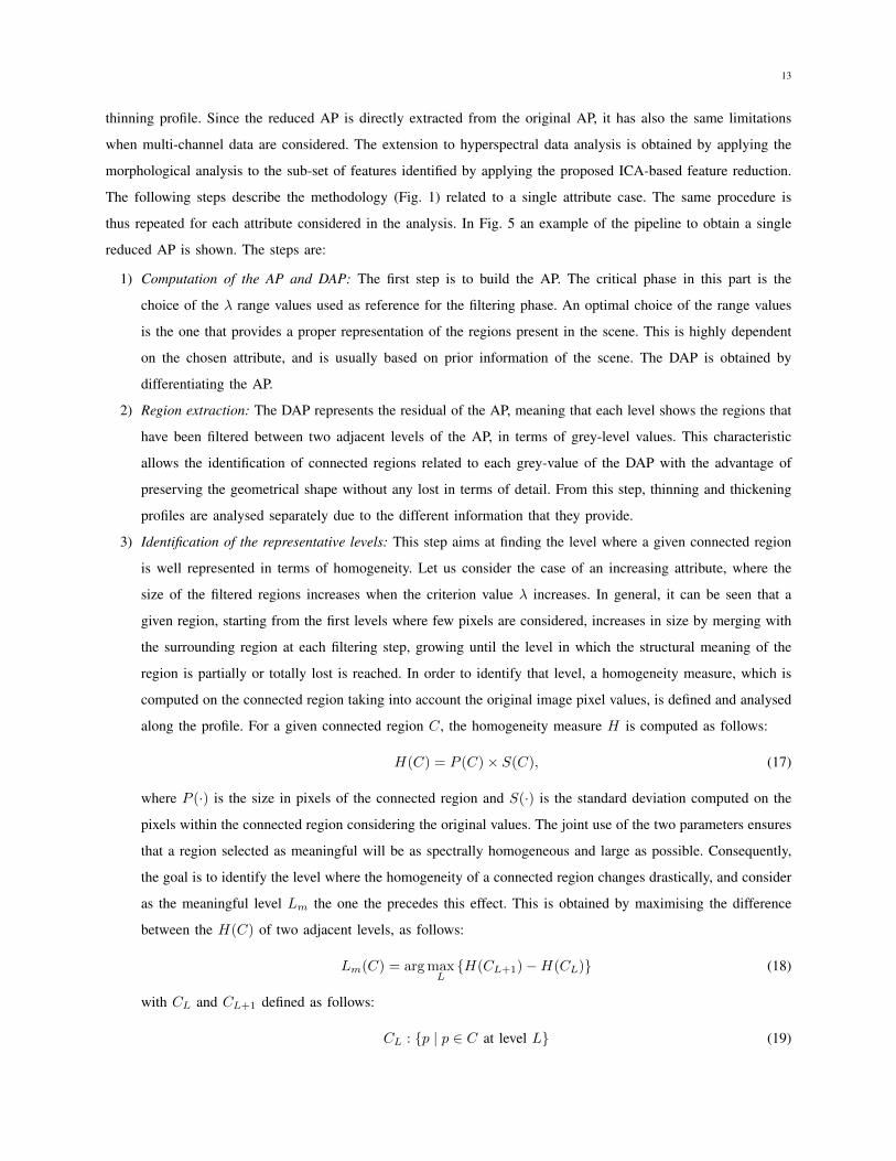
3) Identification of the representative levels: This step aims at finding the level where a given connected region

is well represented in terms of homogeneity. Let us consider the case of an increasing attribute, where the

size of the filtered regions increases when the criterion value � increases. In general, it can be seen that a

given region, starting from the first levels where few pixels are considered, increases in size by merging with

the surrounding region at each filtering step, growing until the level in which the structural meaning of the

region is partially or totally lost is reached. In order to identify that level, a homogeneity measure, which is

computed on the connected region taking into account the original image pixel values, is defined and analysed

along the profile. For a given connected region C, the homogeneity measure H is computed as follows:

H(C) = P (C)⇥ S(C), (17)

where P (·) is the size in pixels of the connected region and S(·) is the standard deviation computed on the

pixels within the connected region considering the original values. The joint use of the two parameters ensures

that a region selected as meaningful will be as spectrally homogeneous and large as possible. Consequently,

the goal is to identify the level where the homogeneity of a connected region changes drastically, and consider

as the meaningful level Lm

the one the precedes this effect. This is obtained by maximising the difference

between the H(C) of two adjacent levels, as follows:

Lm

(C) = arg max

L

{H(CL+1)�H(C

L

)} (18)

with CL

and CL+1 defined as follows:

CL

: {p | p 2 C at level L} (19)

14

CL+1 : {p | p 2 C at level L + 1} (20)

where CL

✓ CL+1. This implies that C

L+1 could be the result of the merging of more connected regions,

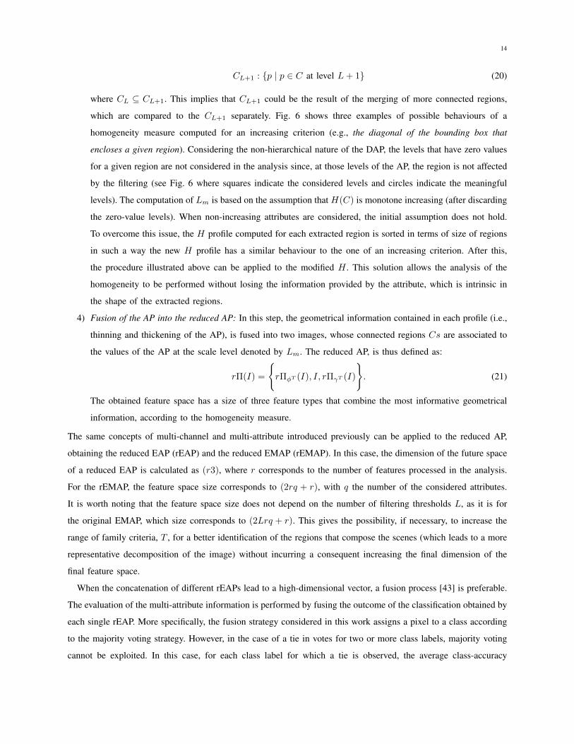
which are compared to the CL+1 separately. Fig. 6 shows three examples of possible behaviours of a

homogeneity measure computed for an increasing criterion (e.g., the diagonal of the bounding box that

encloses a given region). Considering the non-hierarchical nature of the DAP, the levels that have zero values

for a given region are not considered in the analysis since, at those levels of the AP, the region is not affected

by the filtering (see Fig. 6 where squares indicate the considered levels and circles indicate the meaningful

levels). The computation of Lm

is based on the assumption that H(C) is monotone increasing (after discarding

the zero-value levels). When non-increasing attributes are considered, the initial assumption does not hold.

To overcome this issue, the H profile computed for each extracted region is sorted in terms of size of regions

in such a way the new H profile has a similar behaviour to the one of an increasing criterion. After this,

the procedure illustrated above can be applied to the modified H . This solution allows the analysis of the

homogeneity to be performed without losing the information provided by the attribute, which is intrinsic in

the shape of the extracted regions.

4) Fusion of the AP into the reduced AP: In this step, the geometrical information contained in each profile (i.e.,

thinning and thickening of the AP), is fused into two images, whose connected regions Cs are associated to

the values of the AP at the scale level denoted by Lm

. The reduced AP, is thus defined as:

r⇧(I) =

(r⇧

�

T (I), I, r⇧�

T (I)

). (21)

The obtained feature space has a size of three feature types that combine the most informative geometrical

information, according to the homogeneity measure.

The same concepts of multi-channel and multi-attribute introduced previously can be applied to the reduced AP,

obtaining the reduced EAP (rEAP) and the reduced EMAP (rEMAP). In this case, the dimension of the future space

of a reduced EAP is calculated as (r3), where r corresponds to the number of features processed in the analysis.

For the rEMAP, the feature space size corresponds to (2rq + r), with q the number of the considered attributes.

It is worth noting that the feature space size does not depend on the number of filtering thresholds L, as it is for

the original EMAP, which size corresponds to (2Lrq + r). This gives the possibility, if necessary, to increase the

range of family criteria, T , for a better identification of the regions that compose the scenes (which leads to a more

representative decomposition of the image) without incurring a consequent increasing the final dimension of the

final feature space.

When the concatenation of different rEAPs lead to a high-dimensional vector, a fusion process [43] is preferable.

The evaluation of the multi-attribute information is performed by fusing the outcome of the classification obtained by

each single rEAP. More specifically, the fusion strategy considered in this work assigns a pixel to a class according

to the majority voting strategy. However, in the case of a tie in votes for two or more class labels, majority voting

cannot be exploited. In this case, for each class label for which a tie is observed, the average class-accuracy

15

0 2 4 6 8 10 12 14 16 18 200

1

2

3

4

5

6

7

8

9x 10

5

No. levels

Homogeneitymeasu

reH

(a)

1 2 3 4 5 6 7 8 90

1

2

3

4

5

6

7

8

9x 10

5

No. levels (H > 0)

Hom

ogen

eity

mea

sure

H

(c)

0 2 4 6 8 10 12 14 16 18 200

1

2

3

4

5

6

7

8

9x 10

5

No. levels

Homogeneitymeasu

reH

(d)

1 2 3 4 5 60

1

2

3

4

5

6

7

8

9x 10

5

No. levels (H > 0)

Hom

ogen

eity

mea

sure

H

(f)

0 2 4 6 8 10 12 14 16 18 200

1

2

3

4

5

6

7

8

9x 10

5

No. levels

Homogeneitymeasu

reH

(g)

1 2 3 4 5 60

1

2

3

4

5

6

7

8

9x 10

5

No. levels (H > 0)

Hom

ogen

eity

mea

sure

H

(i)

Fig. 6. Examples of homogeneity measure H(C) for an increasing criterion (e.g., diagonal of the bounding box) computed on a given region

C (left column). The levels with zero intensity are not considered in the analysis since the region is not affected by the filtering. The circle

indicates the level Lm

that is chosen (right column).

16

obtained by the classifiers in agreement on the same class label is computed and considered for comparison. The

final decision is made in according to the classifiers that obtained the highest averaged classification accuracy.

IV. EXPERIMENTAL SETUP

A. FastICA Tuning

FastICA is not a parameter-free approach. In our experiments, the non-quadratic function g(u), which represents

the derivative of the non-quadratic function G, is set as tanh(au) with a = 1. This choice provides a good

approximation of negentropy, as proven in [34]. As mentioned in Section II-A2, symmetric orthogonalization is

chosen since in our analysis every feature extracted has the same importance. Moreover, the computation of the ICs

is much faster. Other parameters are related to the stopping criterion. The algorithm stops when the convergence is

reached, meaning that the weight change has to be less than 10

�4, or the maximum number of iterations (which is

set at 1000), is reached. One more parameter is the guess for the initial projection. In order to make the performance

comparison consistent, the identity matrix of size n⇥ n is chosen for initialization.

B. Genetic Algorithm Tuning

A search strategy based on GA is employed to reduce the size of A

opt

by selecting the most representative

column vectors ai

. In this study the classification accuracy obtained by the SVM classifier with the Radial Basis

Function (RBF) kernel is considered as a fitness function to be maximised. However, other measures could be

integrated as fitness function. Since the kernel parameter estimation is computationally expensive, the estimation

is performed once for each population using 5-fold cross-validation. The selection strategy is based on Stochastic

Universal Sampling (SUS) [44], where sigma scaling [42] is employed in order to avoid premature convergence.

The parameters of the GA, such as crossover rate, mutation rate and population size, are determined empirically

through a set of preliminary experiments. In this work, a uniform crossover is used, with a crossover rate of 0.80

and a mutation rate of 0.01. The length of a chromosome is computed as nl, where n is the number of classes of a

specific data set and l is the chosen number of (a

i

, y

T

i

) couples that minimise the reconstruction error. The search

criterion stops when 50 generations are computed.

C. Classification Algorithm

In the experimental analysis, a support vector machine (SVM) classifier is employed for classification purposes,

using a Radial Basis Function (RBF) kernel. The algorithm exploited is the LIBSVM [45] library developed for

MATLAB R�. The one-against-one multi-class strategy is used. For the estimation of the regularization parameter, C,

and the kernel parameter, �, cross-validation based on the grid-search approach is performed. In particular, an expo-

nentially growing sequences of C and � are considered, with C = {10

�2, 10

�1, ..., 10

4} and � = {2

�3, 2�2, ..., 24}.

Each classification result in Section V is obtained by using a 10-fold cross-validation, i.e., that the training set is

split into 10 sets, where 9 of them are used for training the model and the one left is used for validation. In

this way the choice of the parameters results unbiased. For a better understanding of the obtained results, the

17

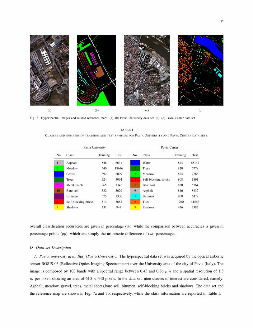
(a) (b) (c) (d)

Fig. 7. Hyperspectral images and related reference maps. (a), (b) Pavia University data set. (c), (d) Pavia Center data set.

TABLE I

CLASSES AND NUMBERS OF TRAINING AND TEST SAMPLES FOR PAVIA UNIVERSITY AND PAVIA CENTER DATA SETS.

Pavia University Pavia Center

No. Class Training Test No. Class Training Test

1 Asphalt 548 6631 1 Water 824 65147

2 Meadow 540 18646 2 Trees 820 6778

3 Gravel 392 2099 3 Meadow 824 2266

4 Trees 524 3064 4 Self-blocking bricks 808 1891

5 Metal sheets 265 1345 5 Bare soil 820 5764

16 Bare soil 532 5029 6 Asphalt 816 8432

7 Bitumen 375 1330 7 Bitumen 808 6479

8 Self-blocking bricks 514 3682 8 Tiles 1260 41566

9 Shadows 231 947 9 Shadows 476 2387

overall classification accuracies are given in percentage (%), while the comparison between accuracies is given in

percentage points (pp), which are simply the arithmetic difference of two percentages.

D. Data set Description

1) Pavia, university area, Italy (Pavia University): The hyperspectral data set was acquired by the optical airborne

sensor ROSIS-03 (Reflective Optics Imaging Spectrometer) over the University area of the city of Pavia (Italy). The

image is composed by 103 bands with a spectral range between 0.43 and 0.86 µm and a spatial resolution of 1.3

m per pixel, showing an area of 610 ⇥ 340 pixels. In the data set, nine classes of interest are considered, namely:

Asphalt, meadow, gravel, trees, metal sheets,bare soil, bitumen, self-blocking bricks and shadows. The data set and

the reference map are shown in Fig. 7a and 7b, respectively, while the class information are reported in Table I.

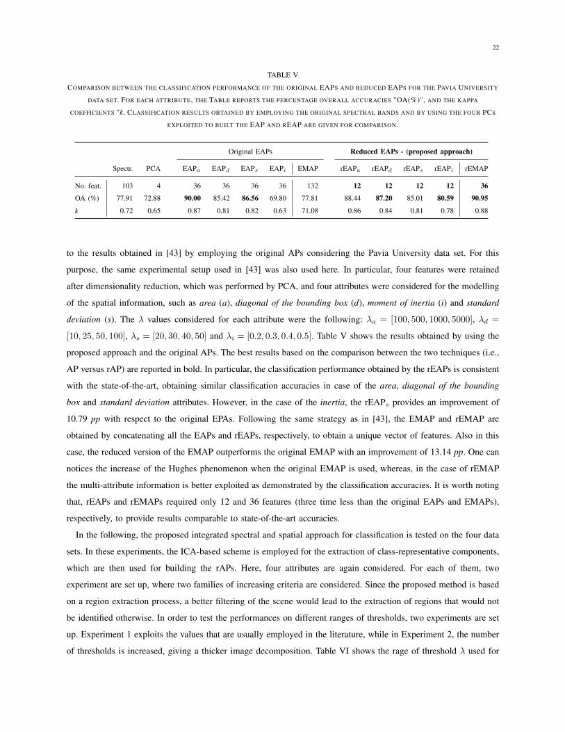
18

(a) (b)

(c)

(d)

Fig. 8. Hyperspectral images (in false color) and related reference maps. (a), (b) Salinas data set. (c), (d) Hekla data set.

TABLE II

CLASSES AND NUMBERS OF TRAINING AND TEST SAMPLES FOR SALINAS AND HEKLA DATA SETS.

Salinas Hekla

No. Class Training Test No. Class Training Test

1 Broccoli green weeds 1 301 1708 1 Andesite lava moss cover 50 973

2 Broccoli green weeds 2 558 3168 2 Scoria 50 500

3 Fallow 296 1680 3 Hyperclatite formation 50 634

4 Fallow rough plow 209 1185 4 Andesite lava 1980 III 50 1446

5 Fallow smooth 401 2277 5 Rhyolite 50 354

6 Stubble 593 3366 6 Andesite lava 1980 I 50 658

7 Celery 536 3043 7 Andesite lava 1991 II 50 360

8 Grapes untrained 1690 9581 8 Andesite lava 1991 I 50 2689

9 Soil vineyard develop 930 5273 9 Firn and glacier ice 50 408

10 Corn senesced green weeds 491 2787 10 Andesite lava 1970 50 292

11 Lettuce romaine 4 weeks 160 908 11 Lava with Tephra and Scoria 50 650

12 Lettuce romaine 5 weeks 289 1638 12 Snow 50 663

13 Lettuce romaine 6 weeks 137 779 - - - -

14 Lettuce romaine 7 weeks 160 910 - - - -

15 Vineyard untrained 1090 6178 - - - -

16 Vineyard vertical trellis 271 1536 - - - -

2) Pavia, central area, Italy (Pavia Center): This scene, as the previous one, was acquired by the ROSIS sensor

during a flight campaign over Pavia. In this case, the data set is composed by 102 spectral bands, with a scene

of 1096 ⇥ 715 pixels. Nine classes of interest are considered, namely: Water, trees, meadow, self-blocking bricks,

19

bare soil, asphalt, bitumen, tiles and shadows. the data set and the related reference map are shown in Fig. 7c and

7d, respectively, while the class information is reported in Table I.

3) Salinas Valley, California (Salinas): The data set has been acquired over Salinas Valley, California, in 1998.

The acquisition has been done by using the AVIRIS (Airborne Visible/Infrared Imaging Spectrometer) sensor, which

uses four spectrometers. The original data set is composed of 224 bands with a spectral range between 0.4 and 2.5

µm. The image has a size of 512 ⇥ 217 pixels with a spatial resolution of 3.7 m. In this study, the corrected data

set is considered by discarding the 20 water absorption bands: [108-112], [154-167], 224. The ground reference

data contains 16 classes of interest (which are described in Table II). The data set and the reference map are shown

in Figs. 8a and 8b. For this data set, the training set used in the experiments is made up of 15% randomly selected

samples from each class.

4) Hekla volcano, Iceland (Hekla): The data set was collected in June 17, 1991 on the active Hekla volcano,

which is located in south-central Iceland, by the 224-band AVIRIS sensor. Due to the failure of the near-infrared

spectrometer (spectrometer 4) during the data acquisition, 64 channels appeared blank. After discarding noisy and

blank channels, the final data set included 157 spectral channels. The image has size of 600 ⇥ 560 pixels with a

geometric resolution of 20 m. It shows mainly lava flows from different eruptions and older hyaloclastites (formed

during subglacial eruptions). The ground reference data contains 12 classes of interests, which are described in

Table II. Figs. 8c and 8d show the image and the reference map, respectively. More information about the data set

can be found in [46]. The training set used here was generated by a random selection of 50 samples from each

class.

V. EXPERIMENTAL RESULTS

A. Spectral Analysis

In this section, the feature dimensionality reduction approach based on ICA (presented in Section III-A), is tested

alone and the obtained results on the four data sets are shown. Aiming at providing a qualitative analysis of the

presented approach, the effectiveness in extracting class-informative features is assessed in terms of classification

accuracies and kappa coefficients. The numerical results are reported in Table III. For each data set, the behaviour

of the proposed approach is tested for a different choice of the parameter l, which indicates the number of the

retained best couples (ai

, yT

i

) that minimise the reconstruction error. The parameter is sets as l = 1, 2, 3, 4. The

proposed approach is then compared to the spectral case, where all the spectral bands are used as input to the

classifier, and to the common strategy based on ICA for feature reduction (i.e., PCA is used as dimensionality

reduction prior to ICA). In the last case, the result shown for each data set represents the best case obtained by

varying the number of components retained from 2 to the spectral dimension. By comparing the obtained results,

one can see that the proposed approach is able to provide representative sub-sets. While this is less evident for

Pavia Center and Salinas, where the classes are already well represented and separated in the spectral case, for the

Pavia University and Hekla data sets, the effectiveness of the proposed approach becomes clearer. In those cases,

significantly higher classification accuracies are achieved for the proposed approach as compared to the spectral

20

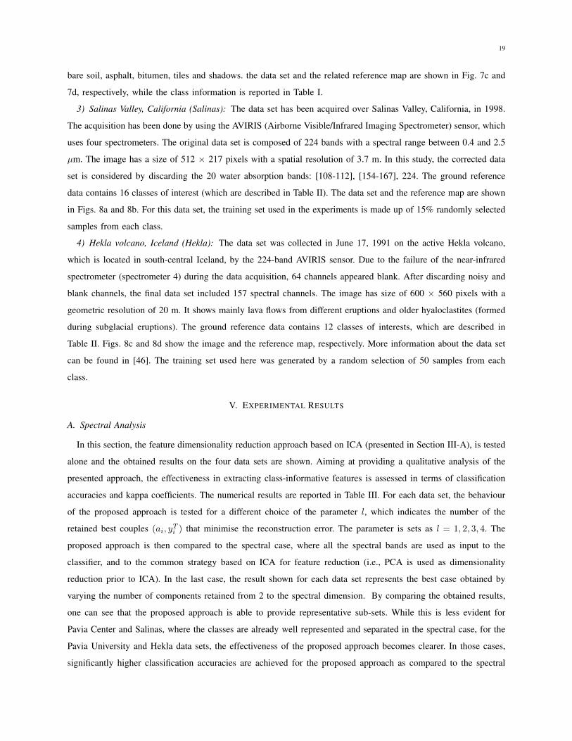
TABLE III

CLASSIFICATION OF THE FOUR DATA SETS BY EMPLOYING THE PROPOSED ICA-BASED FEATURE REDUCTION APPROACH. "NO. FEAT."

DENOTES THE NUMBER OF FEATURES SELECTED BASED ON THE RECONSTRUCTION ERROR, "NO. FEAT. GA" DENOTES THE NUMBER OF

FEATURES AFTER THE GA SELECTION AND USED FOR THE FINAL CLASSIFICATION, "OA (%)" INDICATES THE PERCENTAGE OVERALL

ACCURACIES, "k" INDICATES THE KAPPA COEFFICIENTS AND "STAT." INDICATES THE RESULT OF THE MCNEMAR’S TEST. CLASSIFICATION

RESULTS OBTAINED BY EXPLOITING THE ORIGINAL SPECTRAL BANDS AND BY USING THE PCA-ICA STRATEGY ARE GIVEN FOR

COMPARISON.

Proposed approach

Spectr. PCA-ICA l = 1 l = 2 l = 3 l = 4

Pavia U.

No. feat. 103 12 9 18 27 36

No. feat. GA - - 8 10 10 12

OA (%) 77.91 82.55 79.11 85.25 86.25 87.69

k 0.72 0.78 0.73 0.80 0.82 0.84

Stat. 14.28 -13.16 -19.40 -25.85

Pavia C.

No. feat. 102 8 9 18 27 36

No. feat. GA - - 6 12 17 18

OA (%) 97.35 97.86 97.98 98.17 98.57 98.05

k 0.96 0.97 0.97 0.97 0.98 0.97

Stat. -0.28 -10.44 -21.80 -8.44

Salinas

No. feat. 204 20 16 32 48 64

No. feat. GA - - 13 17 26 29

OA (%) 94.57 94.62 93.71 95.30 95.17 94.93

k 0.91 0.93 0.93 0.95 0.95 0.94

Stat. 8.64 -7.24 -6.06. -5.62

Hekla

No. feat. 157 5 12 24 36 48

No. feat. GA - - 7 12 20 26

OA (%) 93.89 90.40 91.97 94.47 96.28 96.00

k 0.91 0.88 0.91 0.93 0.95 0.95

Stat. -11.62 -13.77 -19.28 -17.96

and the common strategy cases. In particular, for Pavia University, the best classification accuracy is achieved with

l = 4, obtaining after the selection a sub-set of 12 components, with a sharp improvement of 9.78 percentage points

(pp) compared to the spectral case, and of 5.15 pp compared to the best case of PCA-ICA (which is obtained

by extracting 12 features). In the case of Hekla, the best classification accuracy is achieved with l = 3, obtaining

after the selection a sub-set of 20 components. In the Hekla case, the classification accuracy is improved of 5.88

pp compared to the best case of PCA-ICA, and of 2.39 pp compared to the spectral case. In the case of Pavia

Center and Salinas, the best classification accuracies are achieved with l = 3 and l = 2, respectively, retaining

after the selection a sub-set of 17 components with a slight improvement respect to both the spectral case and

PCA-ICA. Table III also reports the results of the McNemar’s test, which is used to asses the statistical significance

of the differences between the results obtained by using the PCA-ICA strategy and the proposed approach. The

21

TABLE IV

COMPARISON OF THE COMPUTATIONAL COSTS FOR THE PROPOSED FEATURE REDUCTION APPROACH BASED ON ICA. THE EXECUTION

TIME OF THE APPROACH IS GIVEN IN SECONDS AS THE SUM OF THE TIME NEEDED FOR THE COMPUTATION AND RANKING OF THE ICS AND

THE SELECTION PERFORMED BY GAS, WHERE "MIN" AND "MAX" INDICATE THE TIME OF THE FASTER AND SLOWER CLASS IN

EXTRACTING THE ICS, WHILE "MEAN" INDICATE THE AVERAGE TIME BETWEEN ALL THE CLASSES.

Proposed approach

single class ICA and rankingSelection (GAs)

PCA-ICA min. max. mean

Pavia U. 3.40 0.05 0.10 0.09 911.92

Pavia C. 4.42 0.06 0.55 0.29 1046.80

Salinas 7.91 0.04 1.45 0.52 1710.43

Hekla 1.87 0.0072 0.0080 0.0075 1191.40

McNemar’s test is based on the standardized normal test statistic, as described in [47]:

Z =

f12 � f21pf12 + f21

, (22)

where f12 represents the samples correctly classified by the strategy 1, represented by the PCA-ICA, and wrongly

by the strategy 2, represented by the proposed approach. The difference in accuracy between the two strategies

can be considered statistically significant if | Z |> 1, 96, while the sign of Z indicates which of the approach

is more accurate. In the case of (Z > 0), the PCA-ICA results are more accurate than those of the proposed

approach, whereas in the case of (Z < 0), the results of the proposed approach are the most accurate. From the

obtained results we can see that all the tests, with the exception of Pavia Center data set for l = 1, are statistically

significant and coherent with the obtained OAs. For this analysis, the computational costs are provided in Table IV.

The execution times are related to the best cases (see the results in bold reported in Table III) obtained by the

proposed feature reduction method based on ICA. Here, the execution time is divided in two components: 1) The

time needed for the computation of ICA and the ranking of the ICs, and 2) the time needed for the last selection

performed by GAs. All the experiments were performed on MATLAB using a computer having Intel Core Duo

2.93-GHz CPU and 4 GB of RAM. As we can see, the computational costs related to the ICA and the ranking of

the ICs are very low and therefore negligible for the final execution times, which are dominated by the GA-based

selection. As aforementioned, the proposed approach could be further optimized by improving the implementation

of the GA-based selection. However, this is not the main goal of the proposed work, which is to propose a strategy

that is able to extract the spectral and spatial information in order to obtain more accurate classification maps,

therefore the high execution times.

B. Spectral and Spatial Analysis

Before to show the results obtained by the proposed spectral and spatial approach, the results obtained in the

previous work [30] are first shown, where the classification performance of the proposed optimisation was compared

22

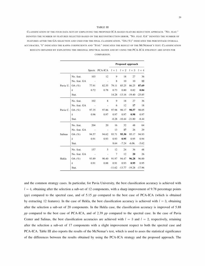
TABLE V

COMPARISON BETWEEN THE CLASSIFICATION PERFORMANCE OF THE ORIGINAL EAPS AND REDUCED EAPS FOR THE PAVIA UNIVERSITY

DATA SET. FOR EACH ATTRIBUTE, THE TABLE REPORTS THE PERCENTAGE OVERALL ACCURACIES "OA(%)", AND THE KAPPA

COEFFICIENTS "k. CLASSIFICATION RESULTS OBTAINED BY EMPLOYING THE ORIGINAL SPECTRAL BANDS AND BY USING THE FOUR PCS

EXPLOITED TO BUILT THE EAP AND REAP ARE GIVEN FOR COMPARISON.

Original EAPs Reduced EAPs - (proposed approach)

Spectr. PCA EAPa

EAPd

EAPs

EAPi

EMAP rEAPa

rEAPd

rEAPs

rEAPi

rEMAP

No. feat. 103 4 36 36 36 36 132 12 12 12 12 36

OA (%) 77.91 72.88 90.00 85.42 86.56 69.80 77.81 88.44 87.20 85.01 80.59 90.95

k 0.72 0.65 0.87 0.81 0.82 0.63 71.08 0.86 0.84 0.81 0.78 0.88

to the results obtained in [43] by employing the original APs considering the Pavia University data set. For this

purpose, the same experimental setup used in [43] was also used here. In particular, four features were retained

after dimensionality reduction, which was performed by PCA, and four attributes were considered for the modelling

of the spatial information, such as area (a), diagonal of the bounding box (d), moment of inertia (i) and standard

deviation (s). The � values considered for each attribute were the following: �a

= [100, 500, 1000, 5000], �d

=

[10, 25, 50, 100], �s

= [20, 30, 40, 50] and �i

= [0.2, 0.3, 0.4, 0.5]. Table V shows the results obtained by using the

proposed approach and the original APs. The best results based on the comparison between the two techniques (i.e.,

AP versus rAP) are reported in bold. In particular, the classification performance obtained by the rEAPs is consistent

with the state-of-the-art, obtaining similar classification accuracies in case of the area, diagonal of the bounding

box and standard deviation attributes. However, in the case of the inertia, the rEAPs

provides an improvement of

10.79 pp with respect to the original EPAs. Following the same strategy as in [43], the EMAP and rEMAP are

obtained by concatenating all the EAPs and rEAPs, respectively, to obtain a unique vector of features. Also in this

case, the reduced version of the EMAP outperforms the original EMAP with an improvement of 13.14 pp. One can

notices the increase of the Hughes phenomenon when the original EMAP is used, whereas, in the case of rEMAP

the multi-attribute information is better exploited as demonstrated by the classification accuracies. It is worth noting

that, rEAPs and rEMAPs required only 12 and 36 features (three time less than the original EAPs and EMAPs),

respectively, to provide results comparable to state-of-the-art accuracies.

In the following, the proposed integrated spectral and spatial approach for classification is tested on the four data

sets. In these experiments, the ICA-based scheme is employed for the extraction of class-representative components,

which are then used for building the rAPs. Here, four attributes are again considered. For each of them, two

experiment are set up, where two families of increasing criteria are considered. Since the proposed method is based

on a region extraction process, a better filtering of the scene would lead to the extraction of regions that would not

be identified otherwise. In order to test the performances on different ranges of thresholds, two experiments are set

up. Experiment 1 exploits the values that are usually employed in the literature, while in Experiment 2, the number

of thresholds is increased, giving a thicker image decomposition. Table VI shows the rage of threshold � used for

23

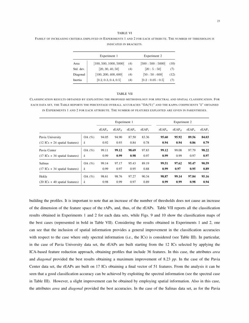
TABLE VI

FAMILY OF INCREASING CRITERIA EMPLOYED IN EXPERIMENTS 1 AND 2 FOR EACH ATTRIBUTE. THE NUMBER OF THRESHOLDS IS

INDICATED IN BRACKETS.

Experiment 1 Experiment 2

Area [100, 500, 1000, 5000] (4) [500 : 500 : 5000] (10)

Std. dev. [20, 30, 40, 50] (4) [20 : 5 : 50] (7)

Diagonal [100, 200, 400, 600] (4) [50 : 50 : 600] (12)

Inertia [0.2, 0.3, 0.4, 0.5] (4) [0.2 : 0.05 : 0.5] (7)

TABLE VII

CLASSIFICATION RESULTS OBTAINED BY EXPLOITING THE PROPOSED METHODOLOGY FOR SPECTRAL AND SPATIAL CLASSIFICATION. FOR

EACH DATA SET, THE TABLE REPORTS THE PERCENTAGE OVERALL ACCURACIES "OA(%)" AND THE KAPPA COEFFICIENTS "k" OBTAINED

IN EXPERIMENTS 1 AND 2 FOR EACH ATTRIBUTE. THE NUMBER OF FEATURES EXPLOITED ARE GIVEN IN PARENTHESES.

Experiment 1 Experiment 2

rEAPa

rEAPd

rEAPs

rEAPi

rEAPa

rEAPd

rEAPs

rEAPi

Pavia University OA (%) 94.05 94.90 87.50 83.36 95.60 95.92 89.56 84.03

(12 ICs + 24 spatial features) k 0.92 0.93 0.84 0.78 0.94 0.94 0.86 0.79

Pavia Center OA (%) 99.11 99.12 98.69 97.83 99.12 99.08 97.79 98.22

(17 ICs + 34 spatial features) k 0.99 0.99 0.98 0.97 0.99 0.99 0.97 0.97

Salinas OA (%) 99.14 97.17 95.43 89.19 99.51 97.62 95.47 90.59

(17 ICs + 34 spatial features) k 0.99 0.97 0.95 0.88 0.99 0.97 0.95 0.89

Hekla OA (%) 98.61 98.76 97.27 90.34 98.87 99.14 97.84 95.16

(20 ICs + 40 spatial features) k 0.98 0.99 0.97 0.89 0.99 0.99 0.98 0.94

building the profiles. It is important to note that an increase of the number of thresholds does not cause an increase

of the dimension of the feature space of the rAPs, and, thus, of the rEAPs. Table VII reports all the classification

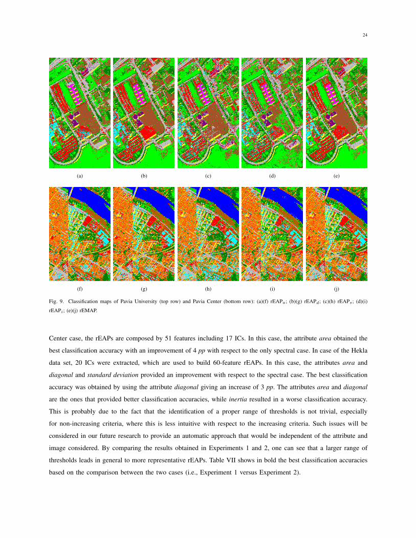
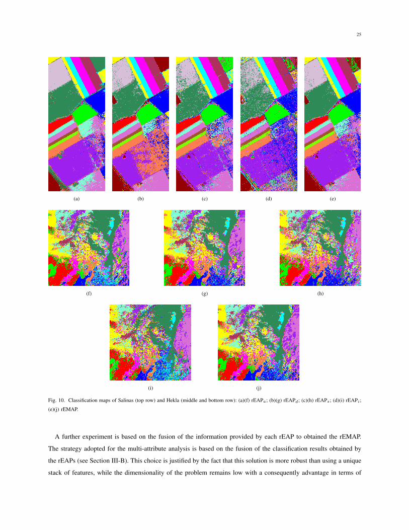
results obtained in Experiments 1 and 2 for each data sets, while Figs. 9 and 10 show the classification maps of

the best cases (represented in bold in Table VII). Considering the results obtained in Experiments 1 and 2, one

can see that the inclusion of spatial information provides a general improvement in the classification accuracies

with respect to the case where only spectral information (i.e., the ICs) is considered (see Table III). In particular,

in the case of Pavia University data set, the rEAPs are built starting from the 12 ICs selected by applying the

ICA-based feature reduction approach, obtaining profiles that include 36 features. In this case, the attributes area

and diagonal provided the best results obtaining a maximum improvement of 8.23 pp. In the case of the Pavia

Center data set, the rEAPs are built on 17 ICs obtaining a final vector of 51 features. From the analysis it can be

seen that a good classification accuracy can be achieved by exploiting the spectral information (see the spectral case

in Table III). However, a slight improvement can be obtained by employing spatial information. Also in this case,

the attributes area and diagonal provided the best accuracies. In the case of the Salinas data set, as for the Pavia

24

(a) (b) (c) (d) (e)

(f) (g) (h) (i) (j)

Fig. 9. Classification maps of Pavia University (top row) and Pavia Center (bottom row): (a)(f) rEAPa

; (b)(g) rEAPd

; (c)(h) rEAPs

; (d)(i)

rEAPi

; (e)(j) rEMAP.

Center case, the rEAPs are composed by 51 features including 17 ICs. In this case, the attribute area obtained the

best classification accuracy with an improvement of 4 pp with respect to the only spectral case. In case of the Hekla

data set, 20 ICs were extracted, which are used to build 60-feature rEAPs. In this case, the attributes area and

diagonal and standard deviation provided an improvement with respect to the spectral case. The best classification

accuracy was obtained by using the attribute diagonal giving an increase of 3 pp. The attributes area and diagonal

are the ones that provided better classification accuracies, while inertia resulted in a worse classification accuracy.

This is probably due to the fact that the identification of a proper range of thresholds is not trivial, especially

for non-increasing criteria, where this is less intuitive with respect to the increasing criteria. Such issues will be

considered in our future research to provide an automatic approach that would be independent of the attribute and

image considered. By comparing the results obtained in Experiments 1 and 2, one can see that a larger range of

thresholds leads in general to more representative rEAPs. Table VII shows in bold the best classification accuracies

based on the comparison between the two cases (i.e., Experiment 1 versus Experiment 2).

25

(a) (b) (c) (d) (e)

(f) (g) (h)

(i) (j)

Fig. 10. Classification maps of Salinas (top row) and Hekla (middle and bottom row): (a)(f) rEAPa

; (b)(g) rEAPd

; (c)(h) rEAPs

; (d)(i) rEAPi

;

(e)(j) rEMAP.

A further experiment is based on the fusion of the information provided by each rEAP to obtained the rEMAP.

The strategy adopted for the multi-attribute analysis is based on the fusion of the classification results obtained by

the rEAPs (see Section III-B). This choice is justified by the fact that this solution is more robust than using a unique

stack of features, while the dimensionality of the problem remains low with a consequently advantage in terms of

26

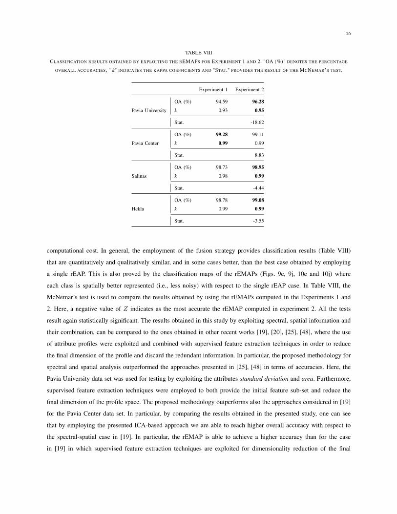
TABLE VIII

CLASSIFICATION RESULTS OBTAINED BY EXPLOITING THE REMAPS FOR EXPERIMENT 1 AND 2. "OA (%)" DENOTES THE PERCENTAGE

OVERALL ACCURACIES, " k" INDICATES THE KAPPA COEFFICIENTS AND "STAT." PROVIDES THE RESULT OF THE MCNEMAR’S TEST.

Experiment 1 Experiment 2

Pavia University

OA (%) 94.59 96.28

k 0.93 0.95

Stat. -18.62

Pavia Center

OA (%) 99.28 99.11

k 0.99 0.99

Stat. 8.83

Salinas

OA (%) 98.73 98.95

k 0.98 0.99

Stat. -4.44

Hekla

OA (%) 98.78 99.08

k 0.99 0.99

Stat. -3.55

computational cost. In general, the employment of the fusion strategy provides classification results (Table VIII)

that are quantitatively and qualitatively similar, and in some cases better, than the best case obtained by employing

a single rEAP. This is also proved by the classification maps of the rEMAPs (Figs. 9e, 9j, 10e and 10j) where

each class is spatially better represented (i.e., less noisy) with respect to the single rEAP case. In Table VIII, the

McNemar’s test is used to compare the results obtained by using the rEMAPs computed in the Experiments 1 and

2. Here, a negative value of Z indicates as the most accurate the rEMAP computed in experiment 2. All the tests

result again statistically significant. The results obtained in this study by exploiting spectral, spatial information and

their combination, can be compared to the ones obtained in other recent works [19], [20], [25], [48], where the use

of attribute profiles were exploited and combined with supervised feature extraction techniques in order to reduce

the final dimension of the profile and discard the redundant information. In particular, the proposed methodology for

spectral and spatial analysis outperformed the approaches presented in [25], [48] in terms of accuracies. Here, the

Pavia University data set was used for testing by exploiting the attributes standard deviation and area. Furthermore,

supervised feature extraction techniques were employed to both provide the initial feature sub-set and reduce the

final dimension of the profile space. The proposed methodology outperforms also the approaches considered in [19]

for the Pavia Center data set. In particular, by comparing the results obtained in the presented study, one can see

that by employing the presented ICA-based approach we are able to reach higher overall accuracy with respect to

the spectral-spatial case in [19]. In particular, the rEMAP is able to achieve a higher accuracy than for the case

in [19] in which supervised feature extraction techniques are exploited for dimensionality reduction of the final

27

profile. In the case of the Pavia University data set, the proposed approach obtained higher accuracies compared

to the case in which the original AP are used, while it provided very close (and in some cases higher) accuracies

to the cases in which feature extraction techniques are exploited. In terms of accuracies, the proposed approach

outperforms also the strategy adopted in [20] considering the case in which standard training set is exploited for

the classification. The reason for such comparison is to prove the effectiveness of both the ICA-based approach

in extracting class-informative features and the reduced APs in providing sub-sets of spatial features in which the

redundant information is discarded. Moreover, the comparison proves that by optimising the information extraction,

the inclusion of additional process steps in the classification chain, such as the multiple use of supervised feature

extraction techniques, can be avoided.

VI. CONCLUSIONS

In this study, a novel methodology for spectral and spatial supervised classification of hyperspectral images was

proposed. The presented methodology optimized the usage of ICA in class-informative feature extraction, while

minimising the disadvantages in the use of APs and its extensions (i.e., EAPs and EMAPs), such as the information

redundancy, which limits the classification capabilities.

In particular, a novel ICA-based feature reduction approach was specially designed to retrieve class-informative

features in a high-dimensionality scenario, i.e., where no prior dimensionality reduction is applied. The selection of

the ICs subset was decided upon the minimization of a criterion function based on the reconstruction error measured

for the ICs extracted from each specific class. A genetic algorithm based approach was employed for the selection of

the final subset. The obtained results confirmed that an appropriate use of ICA can bring prominent improvements

in selecting the most representative components, leading to significantly higher classification accuracies. Moreover,

the proposed schema introduced an automatic approach that non only isolates the most informative features without

any supervision, but also identifies the optimum number of the components to keep.

The analysis was then extended to the spatial information domain with the definition of a novel method for

extracting spatial information. The method was based on a optimized version of attribute profiles, aimed at reducing

both the dimensionality and the redundancy of the information that characterises the APs. The algorithm considered,

built upon multi-scale analysis of the DAP behaviour, resulted in the extraction of geometrical features that

correspond to meaningful structures in the scene at different scales. According to homogeneity criteria, the original

AP was compressed, fusing the most informative geometrical information into few features. The emerged reduced

AP’s feature space accounted for three features types, the reduced thickening and thinning profiles as well as the

original image. Compared against to the original APs, the reduced APs achieved comparable or higher classification

accuracies, while using only few features (i.e., in the presented case was one third of the number of feature of the

original AP). It is worth noting that, in contrast to the original AP, the number of thresholds used in the filtering

process does not affect the final number of features that compose the reduced AP. This property brings important

advantages in the cases of multi-attribute and multi-channel analysis, where the use of reduced EAPs and reduced

EMAPs for modelling the spatial context limits the Hughes phenomenon.

28

The presented methodology was tested on four real hyperspectral images, which were different in spectral / spatial

resolutions and content. The obtained results showed the effectiveness of the proposed methodology in extracting

spectral and spatial features, providing higher or similar accuracies when compared to state of the art.

The experiments carried out pointed out on a series of potential improvements that are promising directions for

future research:

• Considering the proposed feature dimensionality strategy, the definition of an automatic approach for the

estimation of the parameter l, which represents the number of ICs to be retained, would allows us to obtain a

fully automatic and parameter-free approach.

• Considering the morphological tools, their usage could be further optimized by defining an automatic approach

for the identification of the best representative filtering parameters, which is preferable to be independent of

the attribute employed and the image content.

APPENDIX A

ALGORITHM FOR ICS RANKING

Algorithm for the ranking of the couples a

i

, y

T

i

based on the reconstruction error.

1: X X

cl

2: for j 1 to l do

3: for i 1 to m do

4: ei

=

��X� a

i

y

T

i

��2

F

5: end for

6: iopt

= arg min

i

e

7: eopt

= min e

8: X X� a

i

opt

y

T

i

opt

9: a

i

opt

1

10: y

i

opt

1

11: idxj

= iopt

12: e_vecj

= eopt

13: end for

14: return idx, e_vec

ACKNOWLEDGMENT

The authors would like to thank Dr. J. Sigurðsson and Dr. K. Kalimeri for the useful discussion and comments

about this work. This research was in part supported by the research funds of the University of Iceland, in part by

the research funds of the University of Trento, and in part by the European Union’s Seventh Framework Programme

(FP7/2007-2013) Theme Space project North State, under grant agreement n. 606962.

29

REFERENCES

[1] G. F. Hughes, “On the mean accuracy of statistical pattern recognizers,” Information Theory, IEEE Transactions on, vol. 14, no. 1, pp.

55–63, 1968.

[2] K. Fukunaga, Introduction to Statistical Pattern Recognition, 2nd ed., ser. Computer science and scientific computing. Academic Press,

Inc., 1990.

[3] S. Lim, K. Sohn, and C. Lee, “Principal component analysis for compression of hyperspectral images,” in Geoscience and Remote Sensing

Symposium, 2001. IGARSS’01. IEEE 2001 International, vol. 1, 2001, pp. 97–99.

[4] T. Hastie, R. Tibshirani, and J. Friedman, The elements of statistical learning, 2nd ed. Springer, 2009.

[5] A. A. Green, M. Berman, P. Switzer, and M. D. Craig, “A transformation for ordering multispectral data in terms of image quality with

implications for noise removal,” Geoscience and Remote Sensing, IEEE Transactions on, vol. 26, no. 1, pp. 65–74, 1988.

[6] J. Lee, A. Woodyatt, and M. Berman, “Enhancement of high spectral resolution remote-sensing data by a noise-adjusted principal

components transform,” Geoscience and Remote Sensing, IEEE Transactions on, vol. 28, no. 3, pp. 295–304, May 1990.

[7] P. Comon, “Independent component analysis, a new concept?” Signal processing, vol. 36, no. 3, pp. 287 – 314, 1994.

[8] C. Lee and D. A. Landgrebe, “Feature extraction based on decision boundaries,” Pattern Analysis and Machine Intelligence, IEEE

Transactions on, vol. 15, no. 4, pp. 388–400, 1993.

[9] L. O. Jimenez and D. A. Landgrebe, “Hyperspectral data analysis and supervised feature reduction via projection pursuit,” Geoscience

and Remote Sensing, IEEE Transactions on, vol. 37, no. 6, pp. 2653–2667, 1999.

[10] B.-C. Kuo and D. A. Landgrebe, “Nonparametric weighted feature extraction for classification,” Geoscience and Remote Sensing, IEEE

Transactions on, vol. 42, no. 5, pp. 1096–1105, 2004.

[11] T. Marill and D. M. Green, “On the effectiveness of receptors in recognition systems,” Information Theory, IEEE Transactions on, vol. 9,

no. 1, pp. 11–17, 1963.

[12] A. W. Whitney, “A Direct Method of Nonparametric Measurement Selection,” Computers, IEEE Transactions on, vol. C-20, no. 9, pp.

1100–1103, 1971.

[13] P. Pudil, J. Novovicová, and J. Kittler, “Floating search methods in feature selection,” Pattern Recognition Letters, vol. 15, no. 11, pp.

1119–1125, 1994.

[14] S. B. Serpico and L. Bruzzone, “A new search algorithm for feature selection in hyperspectral remote sensing images,” Geoscience and

Remote Sensing, IEEE Transactions on, vol. 39, no. 7, pp. 1360–1367, 2001.

[15] D. E. Goldberg, Genetic Algorithms in Search, Optimization and Machine Learning. Boston: Addison-Wesley Longman Publishing Co.,

Inc., 1989.

[16] L. Bruzzone and B. Demir, “A Review of Modern Approaches to Classification of Remote Sensing Data,” in Land Use and Land Cover

Mapping in Europe, ser. Remote Sensing and Digital Image Processing, I. Manakos and M. Braun, Eds. Springer Netherlands, 2014,

vol. 18, pp. 127–143.

[17] M. Dalla Mura, J. A. Benediktsson, B. Waske, and L. Bruzzone, “Morphological Attribute Profiles for the Analysis of Very High Resolution

Images,” Geoscience and Remote Sensing, IEEE Transactions on, vol. 48, no. 10, pp. 3747–3762, 2010.

[18] ——, “Extended profiles with morphological attribute filters for the analysis of hyperspectral data,” International Journal of Remote

Sensing, vol. 31, no. 22, pp. 5975–5991, Dec. 2010.

[19] P. Ghamisi, J. A. Benediktsson, and J. R. Sveinsson, “Automatic SpectralâASSpatial Classification Framework Based on Attribute Profiles

and Supervised Feature Extraction,” Geoscience and Remote Sensing, IEEE Transactions on, pp. 1–12, 2013.

[20] S. Bernabe, P. R. Marpu, A. Plaza, M. D. Mura, and J. A. Benediktsson, “SpectralâASSpatial Classification of Multispectral Images Using

Kernel Feature Space Representation,” Geoscience and Remote Sensing Letters, IEEE, vol. 11, no. 1, pp. 288–292, Jan. 2014.

[21] M. Pesaresi and J. A. Benediktsson, “A new approach for the morphological segmentation of high-resolution satellite imagery,” Geoscience

and Remote Sensing, IEEE Transactions on, vol. 39, no. 2, pp. 309–320, 2001.

[22] N. Falco, M. Dalla Mura, F. Bovolo, J. A. Benediktsson, and L. Bruzzone, “Change Detection in VHR Images Based on Morphological

Attribute Profiles,” Geoscience and Remote Sensing Letters, IEEE, vol. 10, no. 3, pp. 636–640, May 2013.

[23] E. J. Breen and R. Jones, “Attribute Openings, Thinnings, and Granulometries,” Computer Vision and Image Understanding, vol. 64, no. 3,

pp. 377–389, Nov. 1996.

30

[24] J. A. Benediktsson, M. Pesaresi, and K. Arnason, “Classification and Feature Extraction for Remote Sensing Images From Urban Areas

Based on Morphological Transformations,” Geoscience and Remote Sensing, IEEE Transactions on, vol. 41, no. 9, pp. 1940–1949, Sep.

2003.

[25] P. R. Marpu, M. Pedergnana, M. D. Mura, S. Peeters, J. A. Benediktsson, and L. Bruzzone, “Classification of hyperspectral data using

extended attribute profiles based on supervised and unsupervised feature extraction techniques,” International Journal of Image and Data

Fusion, vol. 3, no. 3, pp. 269–298, Sep. 2012.

[26] M. Pesaresi, G. K. Ouzounis, and L. Gueguen, “A new compact representation of morphological profiles: report on first massive VHR

image processing at the JRC,” in SPIE Defense, Security, and Sensing, S. S. Shen and P. E. Lewis, Eds., vol. 8390. International Society

for Optics and Photonics, May 2012, pp. 839 025–839 025–6.

[27] J. M. Bioucas-Dias and M. A. T. Figueiredo, “Alternating direction algorithms for constrained sparse regression: Application to hyperspectral

unmixing,” in Hyperspectral Image and Signal Processing: Evolution in Remote Sensing (WHISPERS), 2010 2nd Workshop on. IEEE,

Jun. 2010, pp. 1–4.

[28] B. Song, M. Dalla Mura, P. Li, A. J. Plaza, J. M. Bioucas-Dias, J. A. Benediktsson, and J. Chanussot, “Remotely Sensed Image Classification

Using Sparse Representations of Morphological Attribute Profiles,” Geoscience and Remote Sensing, IEEE Transactions on, vol. 52, no. 8,

pp. 5122–5136, Aug. 2014.

[29] N. Falco, L. Bruzzone, and J. A. Benediktsson, “An ICA based approach to hyperspectral image feature reduction,” in Geoscience and

Remote Sensing Symposium, 2014. IGARSS 2014. IEEE International. IEEE, Jul. 2014, pp. 3470–3473.

[30] N. Falco, J. A. Benediktsson, and L. Bruzzone, “Extraction of spatial features in hyperspectral images based on the analysis of differential

attribute profiles,” in Remote Sensing, vol. 8892. International Society for Optics and Photonics, Oct. 2013, p. 88920O.

[31] A. Hyvärinen, “Fast and robust fixed-point algorithms for independent component analysis.” Neural Networks, IEEE Transactions on,

vol. 10, no. 3, pp. 626–34, Jan. 1999. [Online]. Available: http://research.ics.aalto.fi/ica/fastica/

[32] J.-F. Cardoso and A. Souloumiac, “Blind beamforming for non-Gaussian signals,” Radar and Signal Processing, IEE Proceedings F, vol.

140, no. 6, pp. 362–370, 1993. [Online]. Available: http://perso.telecom-paristech.fr/~cardoso/guidesepsou.html

[33] A. J. Bell and T. J. Sejnowski, “An Information-Maximization Approach to Blind Separation and Blind Deconvolution,” Neural

Computation, vol. 7, no. 6, pp. 1129–1159, Nov. 1995.

[34] A. Hyvärinen, J. Karhunen, and E. Oja, Independent Component Analysis. John Wiley & Sons, Inc., 2001.

[35] P. Soille, Morphological Image Analysis, 2nd ed. Berlin, Heidelberg: Springer Berlin Heidelberg, 2004.

[36] J. Serra, Image Analysis and Mathematical Morphology. London: Academic Press, Inc., Jun. 1982.

[37] J. A. Benediktsson, J. A. Palmason, and J. R. Sveinsson, “Classification of Hyperspectral Data From Urban Areas Based on Extended

Morphological Profiles,” Geoscience and Remote Sensing, IEEE Transactions on, vol. 43, no. 3, pp. 480–491, Mar. 2005.

[38] A. Cheriyadat and L. M. Bruce, “Why principal component analysis is not an appropriate feature extraction method for hyperspectral

data,” in Geoscience and Remote Sensing Symposium, 2003. IGARSS 2003. IEEE International, 2003, pp. 3420–3422.

[39] Q. Du, I. Kopriva, and H. Szu, “Independent-component analysis for hyperspectral remote sensing imagery classification,” Optical

Engineering, vol. 45, no. 1, pp. 017 008–1 – 017 008–13, Jan. 2006.

[40] N. Falco, J. A. Benediktsson, and L. Bruzzone, “A Study on the Effectiveness of Different Independent Component Analysis Algorithms

for Hyperspectral Image Classification,” Selected Topics in Applied Earth Observations and Remote Sensing, IEEE Journal of, vol. 7,

no. 6, pp. 2183–2199, Jun. 2014.

[41] J. H. Holland, Adaptation in natural and artificial systems: an introductory analysis with applications to biology, control, and artificial

intelligence. U Michigan Press, 1975.

[42] M. Mitchell, An introduction to genetic algorithms. MIT Press, 1998.

[43] M. Dalla Mura, A. Villa, J. A. Benediktsson, J. Chanussot, and L. Bruzzone, “Classification of Hyperspectral Images by Using Extended

Morphological Attribute Profiles and Independent Component Analysis,” Geoscience and Remote Sensing Letters, IEEE, vol. 8, no. 3, pp.

542–546, 2011.

[44] J. E. Baker, “Reducing bias and inefficiency in the selection algorithm,” in Proceedings of the second international conference on genetic

algorithms, 1987, pp. 14–21.

[45] C.-C. Chang and C.-J. Lin, “LIBSVM: a library for support vector machines,” pp. 1–27, Apr. 2011. [Online]. Available:

http://www.csie.ntu.edu.tw/~cjlin/libsvm/

31

[46] J. A. Benediktsson, J. R. Sveinsson, and K. Árnason, “Classification and feature extraction of AVIRIS data,” Geoscience and Remote

Sensing, IEEE Transactions on, vol. 33, no. 5, pp. 1194–1205, 1995.

[47] G. M. Foody, “Thematic map comparison: evaluating the statistical significance of differences in classification accuracy,” Photogrammetric

Engineering & Remote Sensing Sensing, vol. 70, no. 5, pp. 627–633, 2004.

[48] P. R. Marpu, M. Pedergnana, M. Dalla Mura, J. A. Benediktsson, and L. Bruzzone, “Automatic Generation of Standard Deviation Attribute

Profiles for SpectralâASSpatial Classification of Remote Sensing Data,” Geoscience and Remote Sensing Letters, IEEE, vol. 10, no. 2, pp.

293–297, Mar. 2013.

Nicola Falco (S’10) received his B.Sc. and M.Sc. degrees in telecommunication engineering from the University of

Trento, Trento, Italy, in 2008 and 2011, respectively. From April to October 2011, he served as a Research Assistant

at the Signal Processing Laboratory, at the Faculty of Electrical and Computer Engineering, University of Iceland,

Reykjvík, Iceland. He received his Ph.D. degree in information and communication technologies (telecommunications

area) from the University of Trento and in electrical and computer engineering from the University of Iceland (joint

degree) in 2015. He is currently a Post- Doctoral Researcher at the Signal Processing Laboratory, at the Faculty

of Electrical and Computer Engineering, University of Iceland. His research interests include remote sensing image

processing, mathematical morphology, and pattern recognition, including analysis and classification in hyperspectral imagery, as well as change

detection analysis in optical remote sensing data.

Dr. Falco was a recipient of the Recognition of IEEE GEOSCIENCE REMOTE SENSING LETTERS Best Reviewers in 2013. He serves as a

Reviewer for the IEEE TRANSACTION ON GEOSCIENCE AND REMOTE SENSING, the IEEE GEOSCIENCE AND REMOTE SENSING LETTERS,

the IEEE JOURNAL OF SELECTED TOPIC IN APPLIED EARTH OBSERVATIONS AND REMOTE SENSING, and Pattern Recognition Letters.

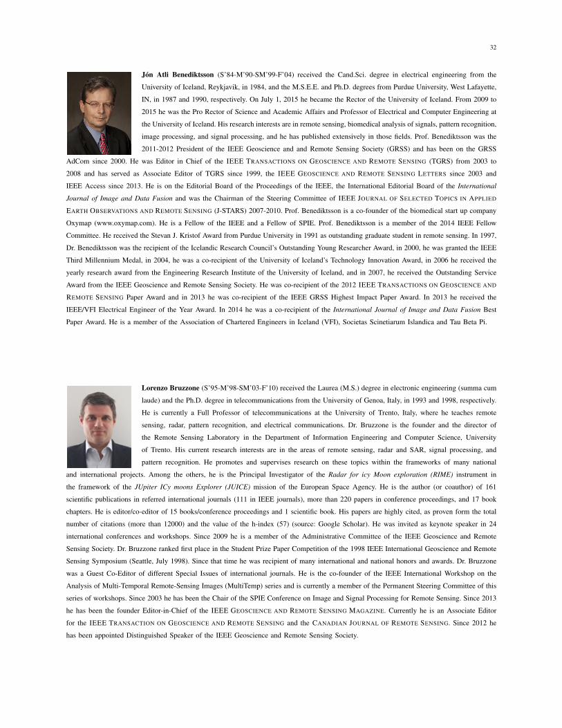
32

Jón Atli Benediktsson (S’84-M’90-SM’99-F’04) received the Cand.Sci. degree in electrical engineering from the

University of Iceland, Reykjavik, in 1984, and the M.S.E.E. and Ph.D. degrees from Purdue University, West Lafayette,

IN, in 1987 and 1990, respectively. On July 1, 2015 he became the Rector of the University of Iceland. From 2009 to

2015 he was the Pro Rector of Science and Academic Affairs and Professor of Electrical and Computer Engineering at

the University of Iceland. His research interests are in remote sensing, biomedical analysis of signals, pattern recognition,

image processing, and signal processing, and he has published extensively in those fields. Prof. Benediktsson was the

2011-2012 President of the IEEE Geoscience and and Remote Sensing Society (GRSS) and has been on the GRSS

AdCom since 2000. He was Editor in Chief of the IEEE TRANSACTIONS ON GEOSCIENCE AND REMOTE SENSING (TGRS) from 2003 to

2008 and has served as Associate Editor of TGRS since 1999, the IEEE GEOSCIENCE AND REMOTE SENSING LETTERS since 2003 and

IEEE Access since 2013. He is on the Editorial Board of the Proceedings of the IEEE, the International Editorial Board of the International

Journal of Image and Data Fusion and was the Chairman of the Steering Committee of IEEE JOURNAL OF SELECTED TOPICS IN APPLIED

EARTH OBSERVATIONS AND REMOTE SENSING (J-STARS) 2007-2010. Prof. Benediktsson is a co-founder of the biomedical start up company

Oxymap (www.oxymap.com). He is a Fellow of the IEEE and a Fellow of SPIE. Prof. Benediktsson is a member of the 2014 IEEE Fellow

Committee. He received the Stevan J. Kristof Award from Purdue University in 1991 as outstanding graduate student in remote sensing. In 1997,

Dr. Benediktsson was the recipient of the Icelandic Research Council’s Outstanding Young Researcher Award, in 2000, he was granted the IEEE

Third Millennium Medal, in 2004, he was a co-recipient of the University of Iceland’s Technology Innovation Award, in 2006 he received the

yearly research award from the Engineering Research Institute of the University of Iceland, and in 2007, he received the Outstanding Service

Award from the IEEE Geoscience and Remote Sensing Society. He was co-recipient of the 2012 IEEE TRANSACTIONS ON GEOSCIENCE AND

REMOTE SENSING Paper Award and in 2013 he was co-recipient of the IEEE GRSS Highest Impact Paper Award. In 2013 he received the

IEEE/VFI Electrical Engineer of the Year Award. In 2014 he was a co-recipient of the International Journal of Image and Data Fusion Best

Paper Award. He is a member of the Association of Chartered Engineers in Iceland (VFI), Societas Scinetiarum Islandica and Tau Beta Pi.

Lorenzo Bruzzone (S’95-M’98-SM’03-F’10) received the Laurea (M.S.) degree in electronic engineering (summa cum

laude) and the Ph.D. degree in telecommunications from the University of Genoa, Italy, in 1993 and 1998, respectively.

He is currently a Full Professor of telecommunications at the University of Trento, Italy, where he teaches remote

sensing, radar, pattern recognition, and electrical communications. Dr. Bruzzone is the founder and the director of

the Remote Sensing Laboratory in the Department of Information Engineering and Computer Science, University

of Trento. His current research interests are in the areas of remote sensing, radar and SAR, signal processing, and

pattern recognition. He promotes and supervises research on these topics within the frameworks of many national

and international projects. Among the others, he is the Principal Investigator of the Radar for icy Moon exploration (RIME) instrument in

the framework of the JUpiter ICy moons Explorer (JUICE) mission of the European Space Agency. He is the author (or coauthor) of 161

scientific publications in referred international journals (111 in IEEE journals), more than 220 papers in conference proceedings, and 17 book

chapters. He is editor/co-editor of 15 books/conference proceedings and 1 scientific book. His papers are highly cited, as proven form the total

number of citations (more than 12000) and the value of the h-index (57) (source: Google Scholar). He was invited as keynote speaker in 24

international conferences and workshops. Since 2009 he is a member of the Administrative Committee of the IEEE Geoscience and Remote

Sensing Society. Dr. Bruzzone ranked first place in the Student Prize Paper Competition of the 1998 IEEE International Geoscience and Remote

Sensing Symposium (Seattle, July 1998). Since that time he was recipient of many international and national honors and awards. Dr. Bruzzone

was a Guest Co-Editor of different Special Issues of international journals. He is the co-founder of the IEEE International Workshop on the

Analysis of Multi-Temporal Remote-Sensing Images (MultiTemp) series and is currently a member of the Permanent Steering Committee of this

series of workshops. Since 2003 he has been the Chair of the SPIE Conference on Image and Signal Processing for Remote Sensing. Since 2013

he has been the founder Editor-in-Chief of the IEEE GEOSCIENCE AND REMOTE SENSING MAGAZINE. Currently he is an Associate Editor

for the IEEE TRANSACTION ON GEOSCIENCE AND REMOTE SENSING and the CANADIAN JOURNAL OF REMOTE SENSING. Since 2012 he

has been appointed Distinguished Speaker of the IEEE Geoscience and Remote Sensing Society.