Energy/Geological Survey of the Netherlands

Princetonlaan 6

3584 CB Utrecht

P.O. Box 80015

3508 TA Utrecht

The Netherlands

www.tno.nl

T +31 88 866 42 56

F +31 88 866 44 75

TNO report

TNO 2015 R10216

DoubletCalc 2D 1.0 User Manual

Date 04 November 2015

Author(s) J.G. Veldkamp, M.P.D. Pluymaekers, J.D.A.M. van Wees

Copy no

No. of copies

Number of pages 38 (incl. appendices)

Number of appendices

Sponsor

Project name KIP Geothermie

Project number 060.14577

All rights reserved.

No part of this publication may be reproduced and/or published by print, photoprint, microfilm or any other means without the previous written consent of TNO.

In case this report was drafted on instructions, the rights and obligations of contracting parties are subject to either the General Terms and Conditions for commissions to TNO, or the relevant agreement concluded between the contracting parties. Submitting the report for inspection to parties who have a direct interest is permitted.

© 2015 TNO

TNO report | TNO 2015 R10216 2 / 38

Summary

DoubletCalc 2D v1.0 (DC2D) is a software tool that is developed by TNO. It enables to calculate the temperature and pressure development around two or more geothermal wells in two dimensions over time. The software aims at bridging the gap between simple 1D prediction tools like TNO's DoubletCalc v1.43 (DC1D, Mijnlieff et al. 2014), and sophisticated 2D and 3D reservoir simulators like Eclipse.

The input of DC2D consists of fixed reservoir parameter values for, and/or 2D maps representing temperature, aquifer depth, aquifer thickness, porosity, net-to-gross, permeability and salinity.

The output of DC2D includes:

- graphs showing pressure, flow rate and temperature at both producer and injector against time,

- 2D grids of pressure and temperature per time step, and optionally viscosity, velocity and subsidence.

TNO report | TNO 2015 R10216 3 / 38

Contents

Summary .................................................................................................................. 2

1 Introduction .............................................................................................................. 4

2 User manual ............................................................................................................. 5

2.1 Installation .................................................................................................................. 5

2.2 Input screen ............................................................................................................... 5

2.3 Tab sheets ................................................................................................................. 7

2.4 Error messages ....................................................................................................... 16

3 DoubletCalc 2D model........................................................................................... 18

3.1 Doublet configuration ............................................................................................... 18

3.2 Theoretical background ........................................................................................... 18

4 Benchmark ............................................................................................................. 20

4.1 Analytical solution .................................................................................................... 20

4.2 Eclipse ..................................................................................................................... 20

4.3 DoubletCalc 1D ........................................................................................................ 24

5 Modelling discontinuities ..................................................................................... 29

6 File formats ............................................................................................................ 31

6.1 Grids ........................................................................................................................ 31

6.2 Settings XML file ...................................................................................................... 33

6.3 Output well file ......................................................................................................... 35

7 References ............................................................................................................. 37

8 Signature ...................................................................... Error! Bookmark not defined.

TNO report | TNO 2015 R10216 4 / 38

1 Introduction

DoubletCalc 2D v1.0 (DC2D) is a software tool that is developed by TNO. It enables to calculate the temperature and pressure development around two or more geothermal wells in two dimensions over time. The software aims at bridging the gap between simple 1D prediction tools like TNO's DoubletCalc v1.43 (DC1D, Mijnlieff et al. 2014), and sophisticated 2D and 3D reservoir simulators like Eclipse.

The major differences between DoubletCalc 2D and DoubletCalc v1.43 are:

- DC2D can handle spatial variation in reservoir properties - DC2D can handle discontinuities like faults - DC2D calculates time series - DC2D does not handle uncertainty in parameter values in a stochastic way like

DoubletCalc v1.43 - DC2D can calculate thermal breakthrough times and the influenced area - DC2D can handle multiple wells (>2), thereby enabling to calculate interference

between various doublets.

The output of DC2D includes:

- graphs showing pressure, flow rate and temperature at both producer and injector against time,

- 2D grids of pressure and temperature per time step, and optionally viscosity, velocity and subsidence.

The anticipated users of DC2D are consultants and doublet operators interested in analysis of the lifetime of the doublet, interference issues with neighbouring doublets, or the effects of discontinuities in the reservoir on the anticipated cooling and pressure development in the reservoir.

The DoubletCalc2D software can be downloaded free of charge from www.nlog.nl under the GNU Lesser General Public License.

TNO report | TNO 2015 R10216 5 / 38

2 User manual

2.1 Installation

DoubletCalc 2D does not require specific installation. The contents of the downloaded ZIP-file must be placed into a folder. The program is executed by doubleclicking the executable JAR-file <DoubletCalc2D_1.0_java7_04nov2015.jar>. Optionally the program can be started by executing the batch file provided in the ZIP file: <start_doubletcalc_2D.bat>. Note that executing the batch file may not work when the software is unpacked in an unmapped network location (i.e., no drive letter is assigned). The user is therefore advised to install the software locally, or to map the network location.

In order to run DoubletCalc 2D, an installation of a recent Java version is required. DoubletCalc was tested with Java versions 7 and 8. Java software can be downloaded for free at http://java.com/.

2.2 Input screen

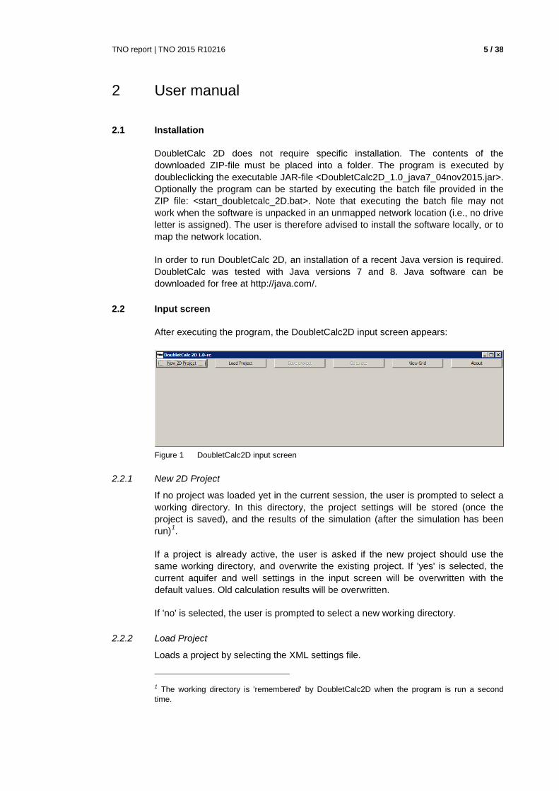
After executing the program, the DoubletCalc2D input screen appears:

Figure 1 DoubletCalc2D input screen

2.2.1 New 2D Project

If no project was loaded yet in the current session, the user is prompted to select a working directory. In this directory, the project settings will be stored (once the project is saved), and the results of the simulation (after the simulation has been run)1.

If a project is already active, the user is asked if the new project should use the same working directory, and overwrite the existing project. If 'yes' is selected, the current aquifer and well settings in the input screen will be overwritten with the default values. Old calculation results will be overwritten.

If 'no' is selected, the user is prompted to select a new working directory.

2.2.2 Load Project

Loads a project by selecting the XML settings file.

1 The working directory is 'remembered' by DoubletCalc2D when the program is run a second time.

TNO report | TNO 2015 R10216 6 / 38

2.2.3 Save Project

Saves the current project as XML settings file.

2.2.4 Calculate

Runs a simulation, and automatically stores, for each time step (year), the resulting temperature and pressure grid files, and the properties calculated for the wells (temperature, pressure, viscosity, density, salinity, compressibility), in the working directory. The output grid format is specified in the Advanced Settings tab (see 2.3.2). The format of the wells files is space delimited, using one line per calculated year and one column per calculated property (see 6.3).

Additional grids can be written when certain settings apply (see the Advanced Settings tab in paragraph 2.3.2).

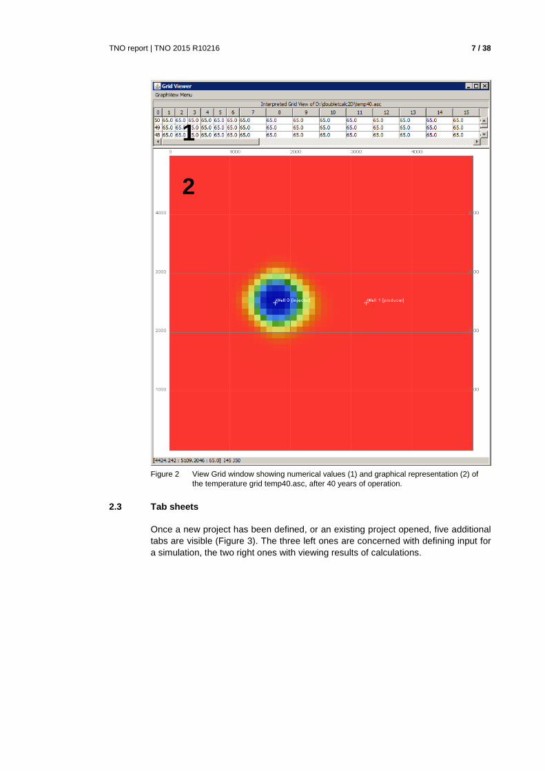
2.2.5 View Grid

Enables to select a single grid for viewing, either results of previous simulations, or grids depicting the aquifer depth, reservoir thickness, etc. The selected grid is opened in the Grid Viewer (Figure 2). The Grid Viewer shows the numerical values of the grid (top part), the grid itself (bottom part) and the well locations. When moving the cursor around, the coordinates of the selected location (X/Y and I/J2 row/column) and corresponding value of the temperature / pressure are shown on the status line of the window. If the cursor is moved around over the grid, the information in the status line is continuously updated. If a cell in the grid is clicked, or if the cursor is moved around over the grid while pressing the left mouse button, the numerical value display on top of the window is updated.

2 I counts columns from left to right, J counts rows from bottom to top

TNO report | TNO 2015 R10216 7 / 38

Figure 2 View Grid window showing numerical values (1) and graphical representation (2) of

the temperature grid temp40.asc, after 40 years of operation.

2.3 Tab sheets

Once a new project has been defined, or an existing project opened, five additional tabs are visible (Figure 3). The three left ones are concerned with defining input for a simulation, the two right ones with viewing results of calculations.

2

1

TNO report | TNO 2015 R10216 8 / 38

Figure 3 DoubletCalc2D input screen for aquifer properties, showing the five tabs in the red

box.

2.3.1 Input aquifer tab

The Input Aquifer tab enables the user to specify

- the Region of Interest (RoI) - the aquifer properties - the calculation settings

2.3.1.1 Region of interest

The region of interest (RoI) is a rectangle defined by the minimum and maximum X and Y coordinates (xmin, xmax, ymin, ymax) and the number of grid cells in the X and Y direction (nx, ny).

Alternatively, by pressing the 'use grid' button to the right of the 'grid geometry', both the 'none' and 'view' buttons to the left and right are activated. Pressing the 'none' button enables to select a grid file. The supported grid formats are ESRI ASCII Grid *.ASC (ESRI), Surfer Grid *.GRD (Golden Software) or Z-Map plus Grid *.DAT (Landmark) format. Examples of the file formats are shown in chapter 6.

Once a grid has been selected, the grid dimensions are read and used for subsequent analysis. The 'none' button text is now replaced by the name of the selected grid, and the 'use grid' button text by 'use values'.

It is possible to view the grid in a basic grid viewer which shows both a map view in a fixed colour scale, and the corresponding numerical values on top.

TNO report | TNO 2015 R10216 9 / 38

The user can switch back to using manually entered values for the RoI by pressing the 'use value' button.

Note that if an ESRI ARC ASCII grid is used for the grid geometry, the coordinates in the file are specified as XLLCORNER and YLLCORNER respectively. These values identical to the manually entered RoI for xmin and ymin. For the other supported grid formats, the coordinates in the grid file are 'cell center' coordinates. Therefore, for an RoI grid having a lower left corner at (0, 0), 100 meter cell size and 50 x 50 rows x columns, the coordinates of the lower left cell are (50, 50) and the upper right cell (4950, 4950) for the SURFER (*.grd) and ZYCOR (*.grd) file formats, while for the equivalent ESRI ASCII grid xllcorner and yllcorner are both 0.

2.3.1.2 Aquifer properties

The aquifer properties the user is requested to enter are specified in Table 1:

parameter unit description initial temperature °C average temperature of the aquifer aquifer depth mTVD depth of the top of the aquifer reservoir thickness m thickness of the aquifer porosity fraction porosity of the aquifer net to gross fraction net to gross ratio of the aquifer actnum - Eclipse code for identifying inactive cells

(value 0). Inactive cells act as flow barrier but not as temperature barrier.

permeability in X and Y mD permeability in the X and Y directions water salinity ppm salinity of the aquifer brine in NaCl

equivalent

Table 1 Aquifer properties

For all parameters except the salinity it is possible to use a 2D grid instead of a fixed value. If the button 'use grid' is pressed, both the 'none' and 'view' buttons to the left and right are activated. Pressing the 'none' button enables to select a grid file. Once a file has been selected, it is possible to view it in a basic grid viewer which shows both a map view in a fixed colour scale, and the corresponding numerical values. The supported grid file formats are the same as can be used for the definition of the RoI.

If the specified grid does not fully cover the RoI, the bounding rows and columns are copied outward until full coverage is achieved. If there is an offset between the grid cells of the RoI and the parameter grid, the parameter grid values are interpolated to the RoI grid cells. The user is therefore strongly advised to use the same grid definition (corner coordinates, number of rows and columns, cellsize) for all input.

If xmin, xmax, ymin, ymax, nx and ny are specified in such a way that the cellsize in the x and y directions (dx, dy) is different, ARC should not be chosen as output file format (paragraph 2.3.2.3). The ARC AsciiGrid format only allow a single value to be specified as cellsize. Therefore calculated grids may not be displayed correctly if dx <> dy.

TNO report | TNO 2015 R10216 10 / 38

Alternatively, the user can switch back to using fixed values by pressing the 'use value' button.

2.3.1.3 Calculation settings

The simulation time settings the user is requested to enter are specified in Table 2:

parameter description time end production number of years the production will continue time end analysis number of years the simulation will calculate output interval grid reporting time step for the production period output/calculation interval after production

grid reporting AND calculation time step for the post-production period

Table 2 Calculation time settings

The 'time end production' can be different from the 'time end analysis' to study – for instance - recovery effects of temperature and pressure after production has ceased. The software always uses one-year time steps for the calculations within the production period, but the 'output interval' time steps determine which temperature and pressure grids will be written to disk. Logically, the 'time end analysis' should be equal to or larger than the 'time end production'.

2.3.2 Advanced settings tab

2.3.2.1 Advanced aquifer properties

The advanced aquifer properties the user is requested to enter are specified in Table 3:

TNO report | TNO 2015 R10216 11 / 38

parameter unit default storage capacity m³/Pa 1.0E-9 water conductivity W/m/K 0.6 temperature dependent viscosity - yes viscosity Pa.s only editable when

'temperature dependent' is switched off

temperature dependent density - yes

Table 3 Advanced aquifer properties

The suggested defaults in Table 3 are considered appropriate values for common situations (Kaye and Laby 1995).

The viscosity can be set to a fixed value if 'temperature dependent viscosity' is switched to 'no'. If it is switched to 'yes' the viscosity is calculated using the correlation given by Batzle and Wang (1992), using the salinity and temperature.

The density is calculated when 'temperature dependent density' is switched to 'yes', by means of the correlation given by Batzle and Wang (1992), using the salinity, temperature and pressure. The contribution to gravity driven flow due to density differences is also accounted for in the flow calculation.

2.3.2.2 Advanced rock properties

The advanced rock properties the user is requested to enter are specified in Table 4. The suggested defaults are considered appropriate values for common rock types (see Bonté 2014 p10, p14 and references therein, and rock properties handbooks like Somerton 1992).

parameter unit default rock thermal conductivity (matrix)3 Wm/K 4 heat capacity J/kg/K 1000 rock density kg/m³ 2700 Young's modulus Pa 9.0E9 Poisson's ratio - 0.35 compaction coefficient bar-1 1.0E-5 thermal compaction coefficient °C-1 2.0E-5

Table 4 Advanced rock properties

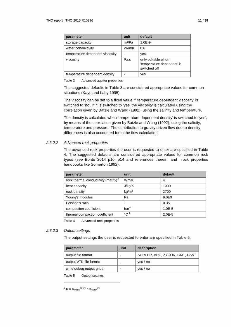
2.3.2.3 Output settings

The output settings the user is requested to enter are specified in Table 5:

parameter unit description

output file format - SURFER, ARC, ZYCOR, GMT, CSV

output VTK file format - yes / no

write debug output grids - yes / no

Table 5 Output settings

3 K = Kmatrix(1-phi) * Kwater

phi

TNO report | TNO 2015 R10216 12 / 38

Pressure and temperature grids are always written to disk for each time step. The file names are pres[year].[ext] and temp[year].[ext]. The user can select the output file format. [ext] can be 'grd' (Surfer), 'asc' (Arc), 'dat' (Zycor), 'txt' (GMT) or 'csv' (CSV). The file formats are described in 6.1.

If 'output VTK file format is set to 'yes' the output is written to ParaView4 Visualisation Toolkit format. This ASCII file format stores all grid information in a single file which can be read by the Paraview visualisation software.

If 'write debug output grids' is set to 'yes', grid output is also written for all input aquifer parameters (depth, thickness, porosity, NG, permeability in X and Y), and initial temperature, fluid velocity and viscosity in X and Y. All grids can be viewed in the Grid Results tab.

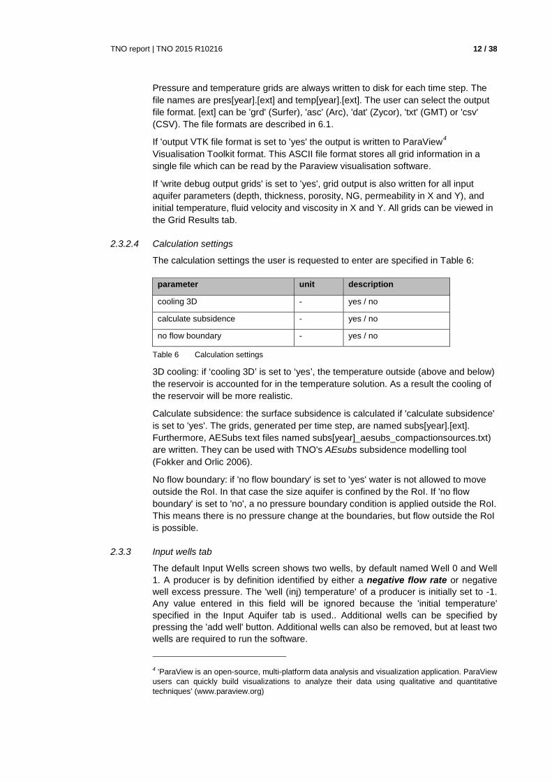
2.3.2.4 Calculation settings

The calculation settings the user is requested to enter are specified in Table 6:

parameter unit description

cooling 3D - yes / no

calculate subsidence - yes / no

no flow boundary - yes / no

Table 6 Calculation settings

3D cooling: if ‘cooling 3D’ is set to ‘yes’, the temperature outside (above and below) the reservoir is accounted for in the temperature solution. As a result the cooling of the reservoir will be more realistic.

Calculate subsidence: the surface subsidence is calculated if 'calculate subsidence' is set to 'yes'. The grids, generated per time step, are named subs[year].[ext]. Furthermore, AESubs text files named subs[year]_aesubs_compactionsources.txt) are written. They can be used with TNO's AEsubs subsidence modelling tool (Fokker and Orlic 2006).

No flow boundary: if 'no flow boundary' is set to 'yes' water is not allowed to move outside the RoI. In that case the size aquifer is confined by the RoI. If 'no flow boundary' is set to 'no', a no pressure boundary condition is applied outside the RoI. This means there is no pressure change at the boundaries, but flow outside the RoI is possible.

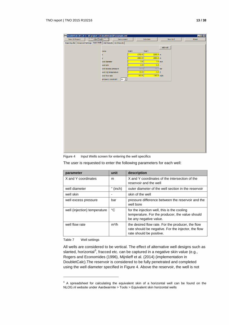
2.3.3 Input wells tab

The default Input Wells screen shows two wells, by default named Well 0 and Well 1. A producer is by definition identified by either a negative flow rate or negative well excess pressure. The 'well (inj) temperature' of a producer is initially set to -1. Any value entered in this field will be ignored because the 'initial temperature' specified in the Input Aquifer tab is used.. Additional wells can be specified by pressing the 'add well' button. Additional wells can also be removed, but at least two wells are required to run the software.

4 'ParaView is an open-source, multi-platform data analysis and visualization application. ParaView users can quickly build visualizations to analyze their data using qualitative and quantitative techniques' (www.paraview.org)

TNO report | TNO 2015 R10216 13 / 38

Figure 4 Input Wells screen for entering the well specifics

The user is requested to enter the following parameters for each well:

parameter unit description X and Y coordinates m X and Y coordinates of the intersection of the

reservoir and the well well diameter " (inch) outer diameter of the well section in the reservoir well skin - skin of the well well excess pressure bar pressure difference between the reservoir and the

well bore well (injection) temperature °C for the injection well, this is the cooling

temperature. For the producer, the value should be any negative value.

well flow rate m³/h the desired flow rate. For the producer, the flow rate should be negative. For the injector, the flow rate should be positive.

Table 7 Well settings

All wells are considered to be vertical. The effect of alternative well designs such as slanted, horizontal5, fracced etc. can be captured in a negative skin value (e.g., Rogers and Economides (1996), Mijnlieff et al. (2014) (implementation in DoubletCalc).The reservoir is considered to be fully penetrated and completed using the well diameter specified in Figure 4. Above the reservoir, the well is not

5 A spreadsheet for calculating the equivalent skin of a horizontal well can be found on the NLOG.nl website under Aardwarmte > Tools > Equivalent skin horizontal wells

TNO report | TNO 2015 R10216 14 / 38

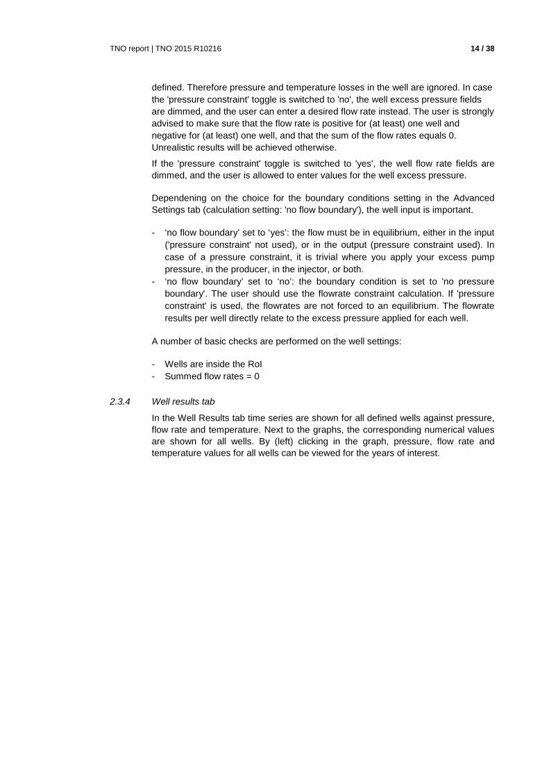
defined. Therefore pressure and temperature losses in the well are ignored. In case the 'pressure constraint' toggle is switched to 'no', the well excess pressure fields are dimmed, and the user can enter a desired flow rate instead. The user is strongly advised to make sure that the flow rate is positive for (at least) one well and negative for (at least) one well, and that the sum of the flow rates equals 0. Unrealistic results will be achieved otherwise.

If the 'pressure constraint' toggle is switched to 'yes', the well flow rate fields are dimmed, and the user is allowed to enter values for the well excess pressure.

Dependening on the choice for the boundary conditions setting in the Advanced Settings tab (calculation setting: 'no flow boundary'), the well input is important.

- ‘no flow boundary’ set to ‘yes’: the flow must be in equilibrium, either in the input ('pressure constraint' not used), or in the output (pressure constraint used). In case of a pressure constraint, it is trivial where you apply your excess pump pressure, in the producer, in the injector, or both.

- ‘no flow boundary’ set to ‘no’: the boundary condition is set to 'no pressure boundary'. The user should use the flowrate constraint calculation. If 'pressure constraint' is used, the flowrates are not forced to an equilibrium. The flowrate results per well directly relate to the excess pressure applied for each well.

A number of basic checks are performed on the well settings:

- Wells are inside the RoI - Summed flow rates = 0

2.3.4 Well results tab

In the Well Results tab time series are shown for all defined wells against pressure, flow rate and temperature. Next to the graphs, the corresponding numerical values are shown for all wells. By (left) clicking in the graph, pressure, flow rate and temperature values for all wells can be viewed for the years of interest.

TNO report | TNO 2015 R10216 15 / 38

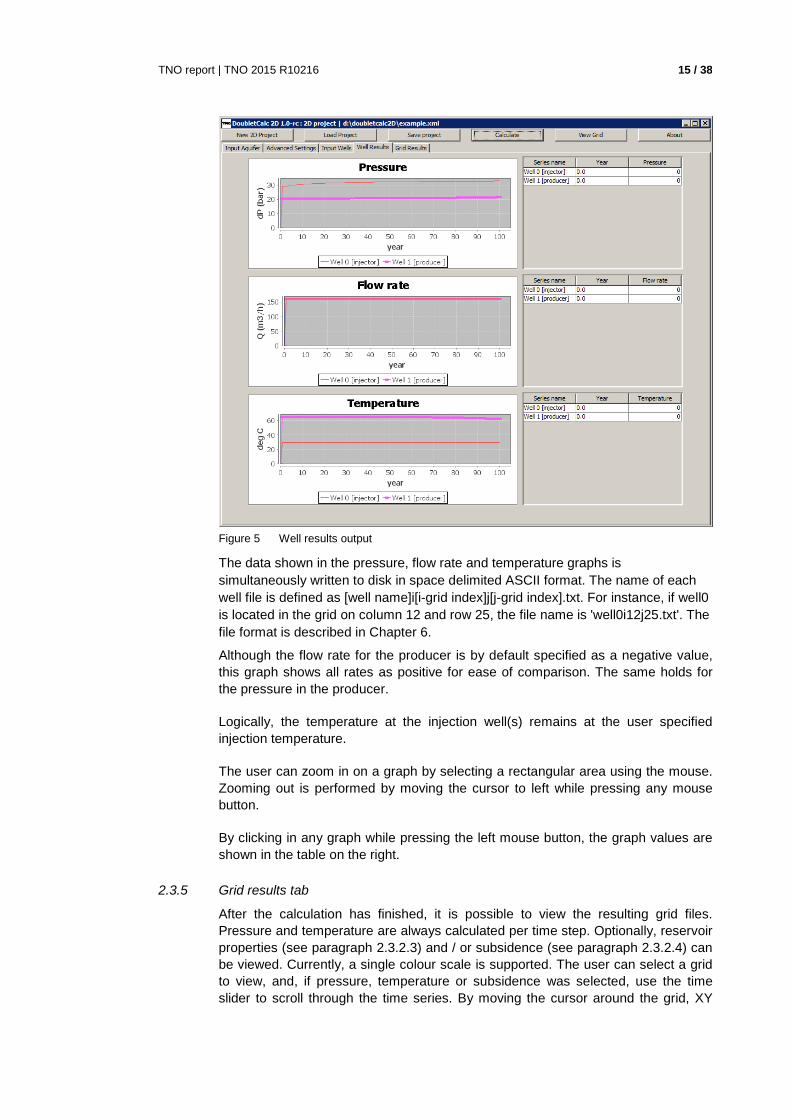
Figure 5 Well results output

The data shown in the pressure, flow rate and temperature graphs is simultaneously written to disk in space delimited ASCII format. The name of each well file is defined as [well name]i[i-grid index]j[j-grid index].txt. For instance, if well0 is located in the grid on column 12 and row 25, the file name is 'well0i12j25.txt'. The file format is described in Chapter 6.

Although the flow rate for the producer is by default specified as a negative value, this graph shows all rates as positive for ease of comparison. The same holds for the pressure in the producer.

Logically, the temperature at the injection well(s) remains at the user specified injection temperature.

The user can zoom in on a graph by selecting a rectangular area using the mouse. Zooming out is performed by moving the cursor to left while pressing any mouse button.

By clicking in any graph while pressing the left mouse button, the graph values are shown in the table on the right.

2.3.5 Grid results tab

After the calculation has finished, it is possible to view the resulting grid files. Pressure and temperature are always calculated per time step. Optionally, reservoir properties (see paragraph 2.3.2.3) and / or subsidence (see paragraph 2.3.2.4) can be viewed. Currently, a single colour scale is supported. The user can select a grid to view, and, if pressure, temperature or subsidence was selected, use the time slider to scroll through the time series. By moving the cursor around the grid, XY

TNO report | TNO 2015 R10216 16 / 38

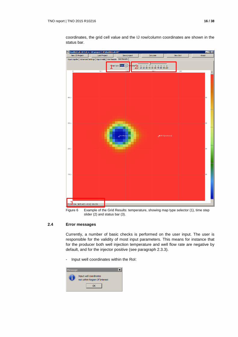
coordinates, the grid cell value and the IJ row/column coordinates are shown in the status bar.

Figure 6 Example of the Grid Results: temperature, showing map type selector (1), time step

slider (2) and status bar (3).

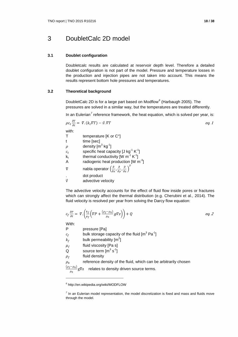
2.4 Error messages

Currently, a number of basic checks is performed on the user input. The user is responsible for the validity of most input parameters. This means for instance that for the producer both well injection temperature and well flow rate are negative by default, and for the injector positive (see paragraph 2.3.3).

- Input well coordinates within the RoI:

1 2

3

TNO report | TNO 2015 R10216 17 / 38

- Production and injection flow rates not in equilibrium:

TNO report | TNO 2015 R10216 18 / 38

3 DoubletCalc 2D model

3.1 Doublet configuration

Doubletcalc results are calculated at reservoir depth level. Therefore a detailed doublet configuration is not part of the model. Pressure and temperature losses in the production and injection pipes are not taken into account. This means the results represent bottom hole pressures and temperatures.

3.2 Theoretical background

DoubletCalc 2D is for a large part based on Modflow6 (Harbaugh 2005). The pressures are solved in a similar way, but the temperatures are treated differently.

In an Eulerian7 reference framework, the heat equation, which is solved per year, is:

𝜌𝜌𝑐𝑐𝑡𝑡𝜕𝜕𝜕𝜕𝜕𝜕𝑡𝑡

= 𝛻𝛻. (𝑘𝑘𝑡𝑡𝛻𝛻𝛻𝛻) − �⃗�𝑣.𝛻𝛻𝛻𝛻 eq. 1

with: T temperature [K or C°] t time [sec] 𝜌𝜌 density [m3 kg-1] 𝑐𝑐𝑡𝑡 specific heat capacity [J kg-1 K-1] kt thermal conductivity [W m-1 K-1] A radiogenic heat production [W m-3]

∇ nabla operator � 𝜕𝜕𝜕𝜕𝜕𝜕

, 𝜕𝜕𝜕𝜕𝜕𝜕

, 𝜕𝜕𝜕𝜕𝜕𝜕

�𝜕𝜕

. dot product v�⃗ advective velocity

The advective velocity accounts for the effect of fluid flow inside pores or fractures which can strongly affect the thermal distribution (e.g. Cherubini et al., 2014). The fluid velocity is resolved per year from solving the Darcy flow equation:

𝑐𝑐𝑓𝑓𝜕𝜕𝜕𝜕𝜕𝜕𝑡𝑡

= 𝛻𝛻.�𝑘𝑘𝑓𝑓𝜇𝜇𝑓𝑓�𝛻𝛻𝛻𝛻 + �𝜌𝜌𝑓𝑓−𝜌𝜌0�

𝜌𝜌0𝑔𝑔𝛻𝛻𝑔𝑔�� + 𝑄𝑄 eq. 2

With: P pressure [Pa] 𝑐𝑐𝑓𝑓 bulk storage capacity of the fluid [m3 Pa-1] 𝑘𝑘𝑓𝑓 bulk permeability [m2] 𝜇𝜇𝑓𝑓 fluid viscosity [Pa s] Q source term [m3 s-1] 𝜌𝜌𝑓𝑓 fluid density 𝜌𝜌0 reference density of the fluid, which can be arbitrarily chosen �𝜌𝜌𝑓𝑓−𝜌𝜌0�

𝜌𝜌0g∇z relates to density driven source terms.

6 http://en.wikipedia.org/wiki/MODFLOW

7 In an Eulerian model representation, the model discretization is fixed and mass and fluids move through the model.

TNO report | TNO 2015 R10216 19 / 38

Through solving the pressure field in eq. 2, the velocities (used for solving the heat equation) can be determined as:

𝑣𝑣𝑓𝑓����⃗ = 𝑘𝑘𝑓𝑓𝜇𝜇𝑓𝑓�𝛻𝛻𝛻𝛻 + �𝜌𝜌𝑓𝑓−𝜌𝜌0�

𝜌𝜌0𝑔𝑔𝛻𝛻𝑔𝑔� eq. 3

For the effect of fluid flow processes on timescales of thousands to millions of years, it is commonly assumed that equation 2 can be solved for a steady-state solution, so that the left hand side of equation 2 is zero.

TNO report | TNO 2015 R10216 20 / 38

4 Benchmark

4.1 Analytical solution

Steady state radial flow in a confined aquifer was described by Thiem (1906). The pressure difference ∆p that has to be applied at either the injector (inj) or producer (prod) in order to produce or inject the required flow rate is:

∆𝑝𝑝𝑖𝑖𝑖𝑖𝑖𝑖 = 𝑄𝑄𝜇𝜇𝑖𝑖𝑖𝑖𝑖𝑖�𝑙𝑙𝑖𝑖�

𝐿𝐿𝑟𝑟𝑤𝑤

�+𝑆𝑆𝑖𝑖𝑖𝑖𝑖𝑖�

2𝜋𝜋𝑘𝑘𝜋𝜋 eq. 4

∆𝑝𝑝𝑝𝑝𝑝𝑝𝑝𝑝𝑝𝑝 = −𝑄𝑄𝜇𝜇𝑝𝑝𝑟𝑟𝑝𝑝𝑝𝑝�𝑙𝑙𝑖𝑖�

𝐿𝐿𝑟𝑟𝑤𝑤

�+𝑆𝑆𝑝𝑝𝑟𝑟𝑝𝑝𝑝𝑝�

2𝜋𝜋𝑘𝑘𝜋𝜋 eq. 5

parameter value unit value SI unit SI permeability k 381 mD 3.76E-13 m2 reservoir thickness H 100 M viscosity μ 0.0008 Pa.s well radius rw 2 " 0.0508 m well rate Q 200 m³/hr 0.0556 m³/s well distance L 900 m

Table 8 Reservoir parameters for analytical solution

When entered in Thiem's equation, the pressure difference at the injector is 18.4 bar (-18.4 at the producer). The DoubletCalc2D solution is very simular, and shown in Figure 7.

Figure 7 DoubletCalc2D pressure solution for the reservoir parameters shown in Table 8.

4.2 Eclipse

A benchmark was carried out using Eclipse8. This paragraph describes the definition of the model used for the benchmark, the assumptions, and the results.

8 Eclipse, developed by Schlumberger, is considered to be the industry reference reservoir simulator.

TNO report | TNO 2015 R10216 21 / 38

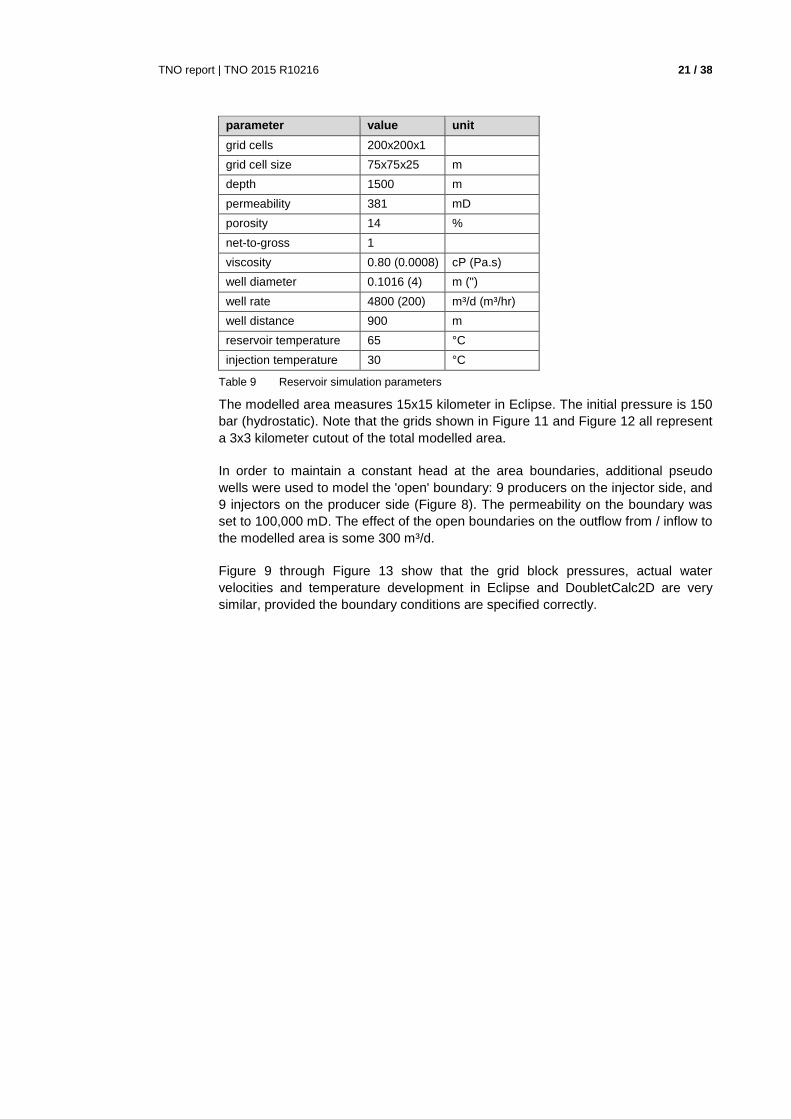
parameter value unit grid cells 200x200x1 grid cell size 75x75x25 m depth 1500 m permeability 381 mD porosity 14 % net-to-gross 1 viscosity 0.80 (0.0008) cP (Pa.s) well diameter 0.1016 (4) m (") well rate 4800 (200) m³/d (m³/hr) well distance 900 m reservoir temperature 65 °C injection temperature 30 °C

Table 9 Reservoir simulation parameters

The modelled area measures 15x15 kilometer in Eclipse. The initial pressure is 150 bar (hydrostatic). Note that the grids shown in Figure 11 and Figure 12 all represent a 3x3 kilometer cutout of the total modelled area.

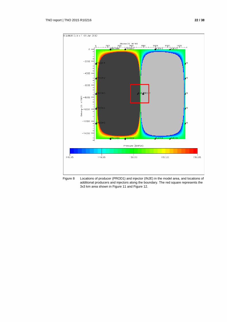
In order to maintain a constant head at the area boundaries, additional pseudo wells were used to model the 'open' boundary: 9 producers on the injector side, and 9 injectors on the producer side (Figure 8). The permeability on the boundary was set to 100,000 mD. The effect of the open boundaries on the outflow from / inflow to the modelled area is some 300 m³/d.

Figure 9 through Figure 13 show that the grid block pressures, actual water velocities and temperature development in Eclipse and DoubletCalc2D are very similar, provided the boundary conditions are specified correctly.

TNO report | TNO 2015 R10216 22 / 38

Figure 8 Locations of producer (PROD1) and injector (INJE) in the model area, and locations of

additional producers and injectors along the boundary. The red square represents the 3x3 km area shown in Figure 11 and Figure 12.

TNO report | TNO 2015 R10216 23 / 38

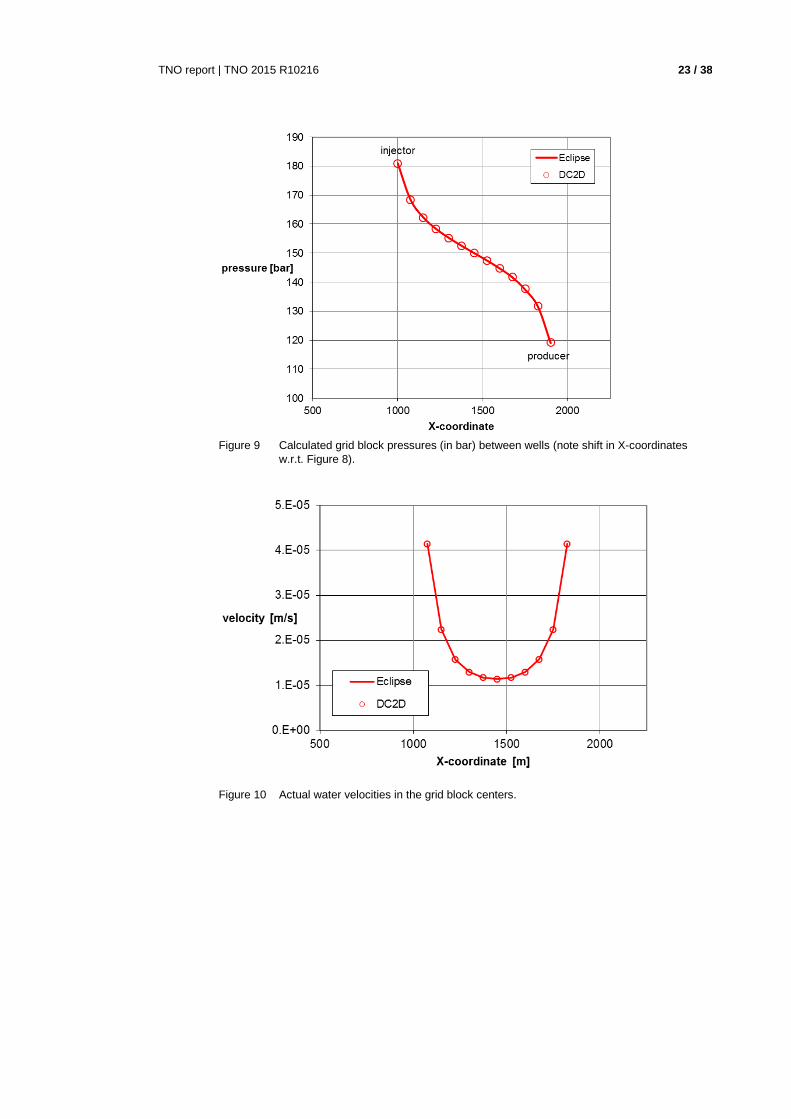
Figure 9 Calculated grid block pressures (in bar) between wells (note shift in X-coordinates

w.r.t. Figure 8).

Figure 10 Actual water velocities in the grid block centers.

TNO report | TNO 2015 R10216 24 / 38

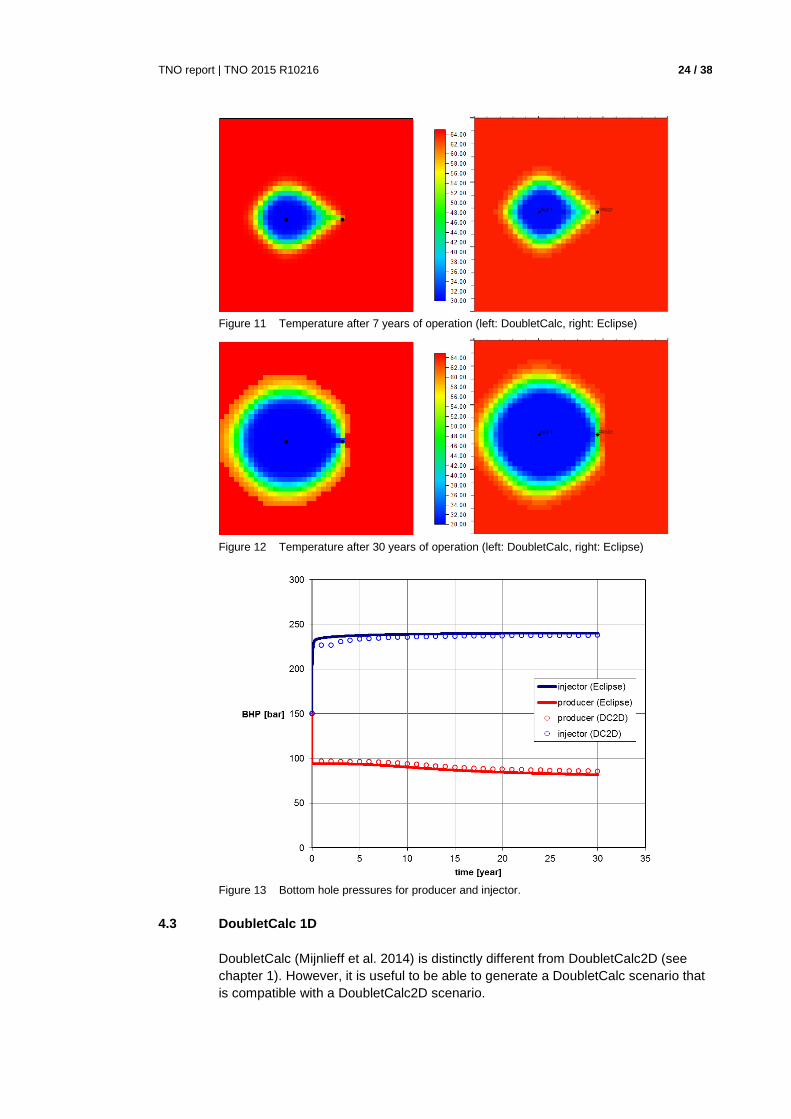
Figure 11 Temperature after 7 years of operation (left: DoubletCalc, right: Eclipse)

Figure 12 Temperature after 30 years of operation (left: DoubletCalc, right: Eclipse)

Figure 13 Bottom hole pressures for producer and injector.

4.3 DoubletCalc 1D

DoubletCalc (Mijnlieff et al. 2014) is distinctly different from DoubletCalc2D (see chapter 1). However, it is useful to be able to generate a DoubletCalc scenario that is compatible with a DoubletCalc2D scenario.

TNO report | TNO 2015 R10216 25 / 38

For that purpose, first a DoubletCalc scenario should be set up according to the planned or realised doublet and reservoir properties. Next, a DoubletCalc2D scenario must be set up as follows:

Input aquifer (Figure 14, Figure 16):

- The region of interest should be defined as the desired study area (not relevant in DoubletCalc).

- The initial temperature should be calculated using the surface temperature, the temperature gradient and the depth of the top of the reservoir specified in DoubletCalc, increased by half the reservoir thickness. This is the wells production temperature.

- The aquifer depth should be the same as specified in DoubletCalc. If the depth varies between producer and injector, a grid should be constructed which represents those depths at the well locations.

- The cell thickness equals the gross reservoir thickness. - The porosity should match the presumed porosity for the area (not relevant in

DoubletCalc). - The net to gross should be the same as specified in DoubletCalc. - The permeability should be the same as specified in DoubletCalc. As

DoubletCalc does not allow the permeability to vary spatially, a grid can not be used. The permeability in the x- and y-directions should be the same.

- The calculation settings for the time should be specified according to the desired period (not relevant in DoubletCalc).

Advanced settings:

- Temperature dependent viscosity and density should be set to 'yes'.

Input well (Figure 14, Figure 15, Figure 17):

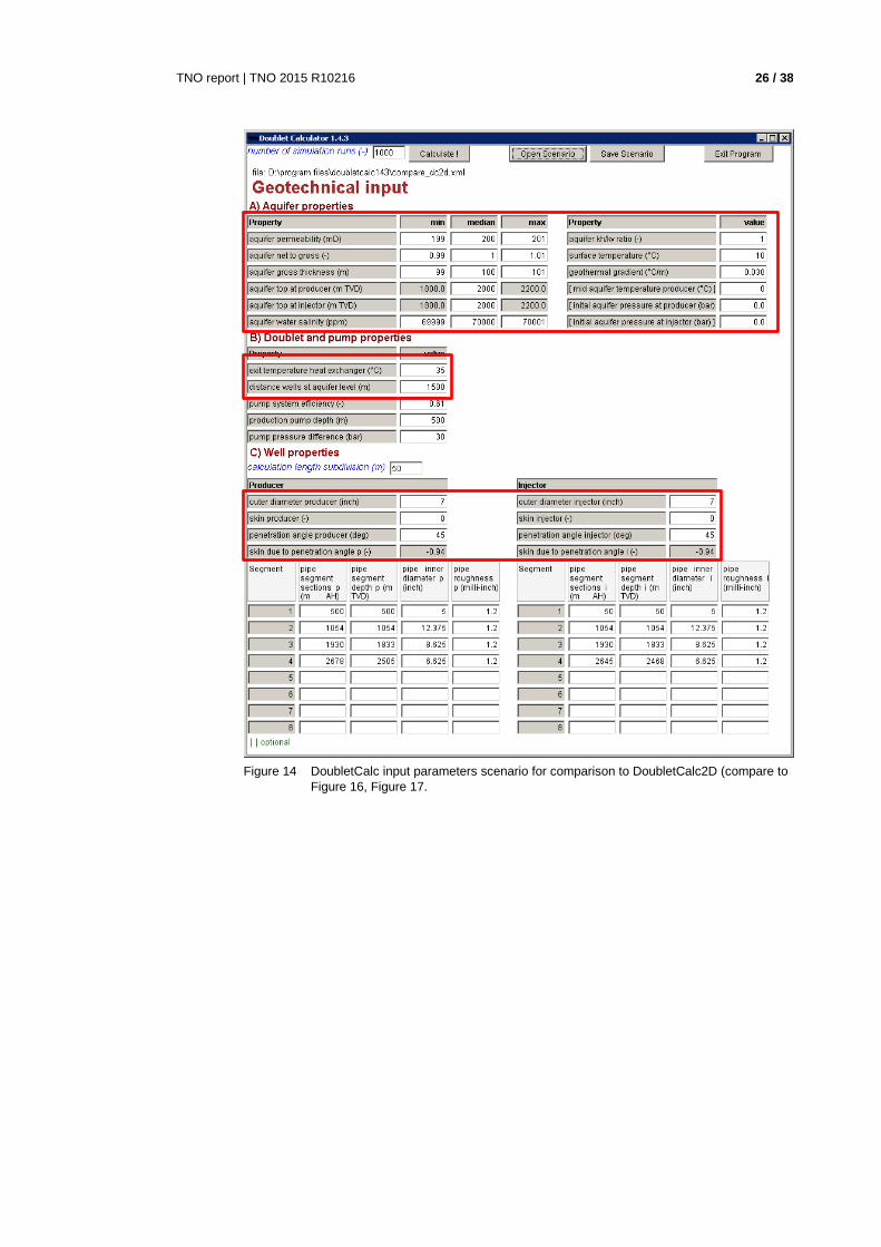
Please take into account that all well input values represent values at reservoir level. As stated in section 3.1 a detailed doublet configuration is not part of the model. Temperature and pressure losses due to friction are ignored. - The X and Y should be chosen in such a way that the distance (at reservoir

level) equals the 'distance wells at aquifer level' in DoubletCalc. - The well diameter should equal the 'outer diameter producer / injector' specified

in DoubletCalc. - The well skin should equal the 'skin producer / injector' plus the 'skin due to

penetration angle' specified in DoubletCalc. - The well (inj) temperature should equal the 'exit temperature at heat exchanger'

specified in DoubletCalc. The temperature of the producer should be set to -1. - The well flow rate for the injector should be set to the value reported by

DoubletCalc as 'pump volume flow' in the DoubletCalc result table. For the producer, the same value should be entered (a negative value by default). Alternatively, the 'pressure constraint' can be set to 'yes'. In that case, instead of the well flow rate the well excess pressures should be specified according to the values for 'pressure difference at producer / injector' in the DoubletCalc result table.

TNO report | TNO 2015 R10216 26 / 38

Figure 14 DoubletCalc input parameters scenario for comparison to DoubletCalc2D (compare to

Figure 16, Figure 17.

TNO report | TNO 2015 R10216 27 / 38

Figure 15 DoubletCalc results screen showing flow rate and pump pressure difference (compare

to Figure 18).

Figure 16 DoubletCalc2D aquifer properties for comparison to DoubletCalc scenario (compare to

Figure 14).

TNO report | TNO 2015 R10216 28 / 38

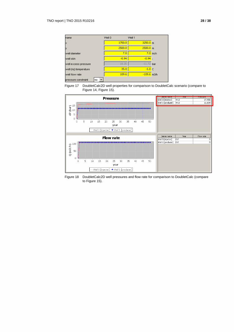
Figure 17 DoubletCalc2D well properties for comparison to DoubletCalc scenario (compare to

Figure 14, Figure 15).

Figure 18 DoubletCalc2D well pressures and flow rate for comparison to DoubletCalc (compare

to Figure 15).

TNO report | TNO 2015 R10216 29 / 38

5 Modelling discontinuities

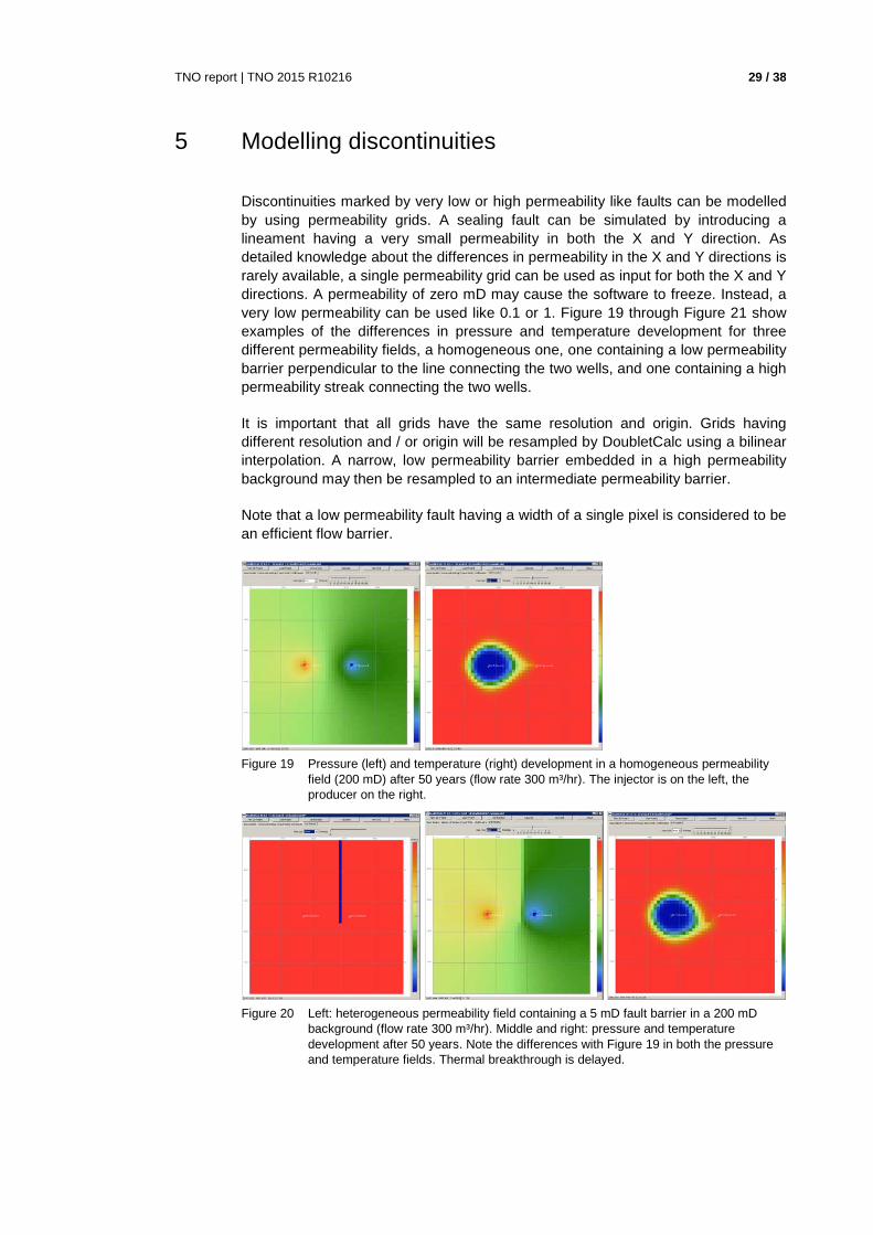
Discontinuities marked by very low or high permeability like faults can be modelled by using permeability grids. A sealing fault can be simulated by introducing a lineament having a very small permeability in both the X and Y direction. As detailed knowledge about the differences in permeability in the X and Y directions is rarely available, a single permeability grid can be used as input for both the X and Y directions. A permeability of zero mD may cause the software to freeze. Instead, a very low permeability can be used like 0.1 or 1. Figure 19 through Figure 21 show examples of the differences in pressure and temperature development for three different permeability fields, a homogeneous one, one containing a low permeability barrier perpendicular to the line connecting the two wells, and one containing a high permeability streak connecting the two wells.

It is important that all grids have the same resolution and origin. Grids having different resolution and / or origin will be resampled by DoubletCalc using a bilinear interpolation. A narrow, low permeability barrier embedded in a high permeability background may then be resampled to an intermediate permeability barrier.

Note that a low permeability fault having a width of a single pixel is considered to be an efficient flow barrier.

Figure 19 Pressure (left) and temperature (right) development in a homogeneous permeability

field (200 mD) after 50 years (flow rate 300 m³/hr). The injector is on the left, the producer on the right.

Figure 20 Left: heterogeneous permeability field containing a 5 mD fault barrier in a 200 mD

background (flow rate 300 m³/hr). Middle and right: pressure and temperature development after 50 years. Note the differences with Figure 19 in both the pressure and temperature fields. Thermal breakthrough is delayed.

TNO report | TNO 2015 R10216 30 / 38

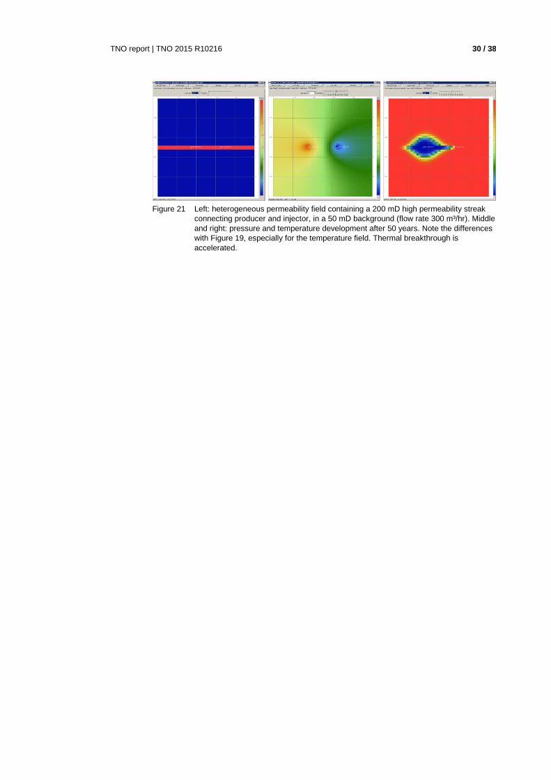
Figure 21 Left: heterogeneous permeability field containing a 200 mD high permeability streak

connecting producer and injector, in a 50 mD background (flow rate 300 m³/hr). Middle and right: pressure and temperature development after 50 years. Note the differences with Figure 19, especially for the temperature field. Thermal breakthrough is accelerated.

TNO report | TNO 2015 R10216 31 / 38

6 File formats

DoubletCalc 2D can export calculation results in various 2D ASCII grid formats for further processing. The formats are described below.

6.1 Grids

6.1.1 Surfer (GRD)

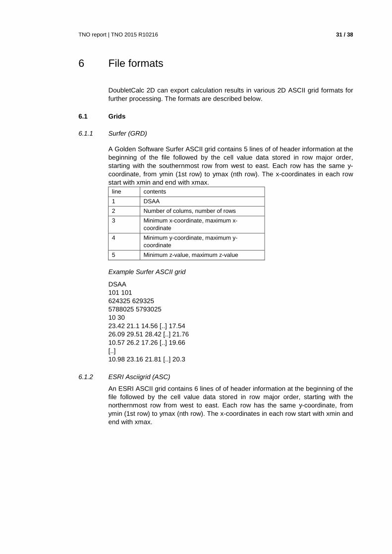
A Golden Software Surfer ASCII grid contains 5 lines of of header information at the beginning of the file followed by the cell value data stored in row major order, starting with the southernmost row from west to east. Each row has the same y-coordinate, from ymin (1st row) to ymax (nth row). The x-coordinates in each row start with xmin and end with xmax.

line contents 1 DSAA 2 Number of colums, number of rows 3 Minimum x-coordinate, maximum x-

coordinate 4 Minimum y-coordinate, maximum y-

coordinate 5 Minimum z-value, maximum z-value

Example Surfer ASCII grid

DSAA 101 101 624325 629325 5788025 5793025 10 30 23.42 21.1 14.56 [..] 17.54 26.09 29.51 28.42 [..] 21.76 10.57 26.2 17.26 [..] 19.66 [..] 10.98 23.16 21.81 [..] 20.3

6.1.2 ESRI Asciigrid (ASC)

An ESRI ASCII grid contains 6 lines of of header information at the beginning of the file followed by the cell value data stored in row major order, starting with the northernmost row from west to east. Each row has the same y-coordinate, from ymin (1st row) to ymax (nth row). The x-coordinates in each row start with xmin and end with xmax.

TNO report | TNO 2015 R10216 32 / 38

line parameter description requirements

1 NCOLS number of cell columns integer greater than 0

2 NROWS number of cell rows integer greater than 0

3 XLLCENTER or XLLCORNER

X coordinate of the origin (by center or lower left corner of the cell).

match with Y coordinate type

4 YLLCENTER or YLLCORNER

Y coordinate of the origin (by center or lower left corner of the cell)

match with X coordinate type

5 CELLSIZE cell size greater than 0

6 NODATA_VALUE the input values to be NoData in the output raster

optional. Default is -9999

Example ESRI ASCII grid:

ncols 101 nrows 101 xllcorner 624300 yllcorner 5788000 cellsize 50 nodata_value -9999 10.98 23.16 21.81 [..] 20.30 27.70 22.54 13.96 [..] 29.48 10.40 26.87 22.26 [..] 25.64 [..] 23.42 21.10 14.56 [..] 17.54

6.1.3 Zycor (ZMap+)

A Landmark ZYCOR Zmap+ ASCII grid contains 5 lines of of header information at the beginning of the file. The header both starts and ends with the '@' character. Optionally the header is preceded by a number of comment lines all starting with '!'). The header is followed by the cell value data stored in column major order, starting with the westernmost column from north to south. The number of cell values per line does not exceed the last number in the first header line.

line parameter description

1 '@', user defined text, 'GRID' keyword, maximum number of cell values per line

2 '15', no data value, empty field, '1', '1'

3 number of columns, number of rows, minimum and maximum x-coordinates, minimum and maximum y-coordinates

4 cell size in x-direction, cell size in y-direction, cell size in z-direction

Example Zycor ZMAP+ ASCII grid:

@testgrid_out.asc HEADER, GRID, 5 15, 0.1000000E+31 , ,7, 1 101, 101, 624325, 629325, 5788025, 5793025 50, 50 @ 10.98 23.16 21.81 [..] 20.30

TNO report | TNO 2015 R10216 33 / 38

27.70 22.54 13.96 [..] 29.48 10.40 26.87 22.26 [..] 25.64 [..] 23.42 21.10 14.56 [..] 17.54

6.1.4 GMT

The open source GMT format is space delimited ASCII file containing three columns X, Y and the pixel value. No header information is provided.

Example GMT file

624325.0 5788025.0 23.42 624375.0 5788025.0 21.1 624425.0 5788025.0 14.559999

6.1.5 CSV

The CSV format is a comma delimited ASCII file containing four columns X, Y and Z for the cell coordinates, and the pixel value. The file starts with 1 line of of header information followed by the cell value data stored in row major order, starting with the southernmost row from west to east, one cell per line. Z is the depth of the middle of the aquifer (top + thickness / 2).

Example CSV file

x, y, z, value 624325.0, 5788025.0, -1511.71, 23.42 624375.0, 5788025.0, -1510.55, 21.1 624425.0, 5788025.0, -1507.28, 14.559999

6.2 Settings XML file

The DoubletCalc 2D project settings specified in the 'Input Aquifer', 'Advanced Settings' and 'Input Wells' tabs are all stored in an XML file. The file starts with two lines identifying the XML-version and the project type_id (currently: 2).

<?xml version="1.0" encoding="UTF-8" standalone="no"?> <project type_id="2">

settings go here </project>

The field descriptions shown below are considered to be mostly self-explaining. For each variable to be entered there is a line in the XML file, identified by the keyword. The value of the variable is filled in between the keyword:

<nx>101</nx>

For parameters that can be defined as grid file (such as all aquifer properties except the salinity), three values are stored in the XML: the (default) numerical value, a value that can be either 0 or 1, and the grid file name. If a numerical value is to be used, the middle value is set to 0. If a grid is to be used, it is 1 and the grid file

TNO report | TNO 2015 R10216 34 / 38

name should be specified. If no grid file has been specified, the latter is set to 'none'.

Yes / no toggles like 'use temperature dependent viscosity' are coded with yes = 1 and no = 0.

6.2.1 Input aquifer tab

Region of interest parameters:

<nx>50.0</nx> <xmin>5000.0</xmin> <xmax>5000.0</xmax> <ny>50.0</ny> <ymin>0.0</ymin> <ymax>0.0</ymax> <nz>10.0</nz> <zmin>0.0</zmin> <zmax>0.0</zmax> <grid_geometry>0.0 0 none</grid_geometry>

Aquifer properties parameters:

<initial_temperature>65.0 0 none</initial_temperature> <aquifer_depth>1500.0 0 none</aquifer_depth> <_cell__thickness>100.0 0 none</_cell__thickness> <porosity>0.12 0 none</porosity> <net_to_gross>1.0 0 none</net_to_gross> <actnum>1.0 0 none</actnum> <permeability_in_xdir>200.0 0 none</permeability_in_xdir> <permeability_in_ydir>200.0 0 none</permeability_in_ydir> <permeability_in_kdir>200.0 0 none</permeability_in_kdir> <water_salinity>70000.0</water_salinity>

Calculation settings parameters:

<time_end_production>15.0</time_end_production> <time_end_analysis>15.0</time_end_analysis> <output_interval>1.0</output_interval> <output_calculation_interval_after_production>250.0</output_calculation_interval_a

fter_production>

6.2.2 Advanced settings tab

Advanced aquifer properties parameters:

<storage_capacity>1.0E-9</storage_capacity> <water_conductivity>0.6</water_conductivity> <temperature_dependent_viscosity>1.0</temperature_dependent_viscosity> <temperature_dependent_density>1.0</temperature_dependent_density> <viscosity>0.001 0 none</viscosity>

Advanced rock properties parameters:

<rock_conductivity>4.0</rock_conductivity> <heat_capacity>1000.0</heat_capacity>

TNO report | TNO 2015 R10216 35 / 38

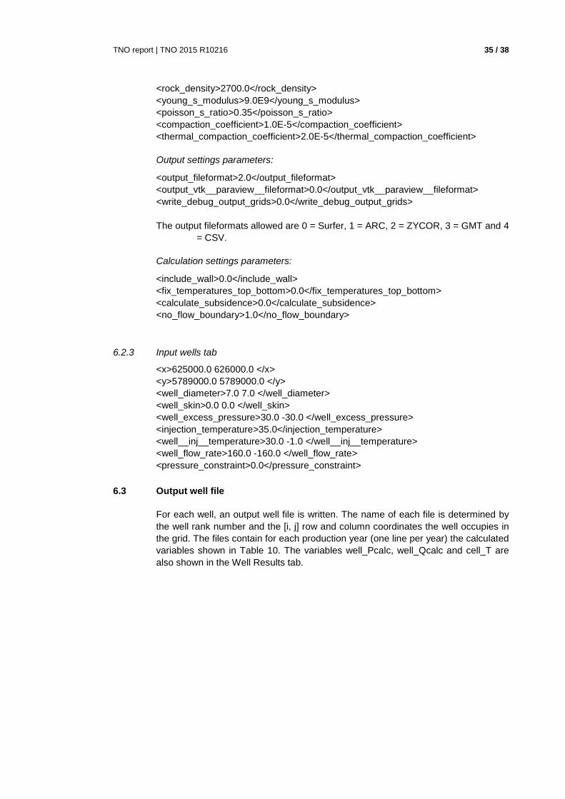
<rock_density>2700.0</rock_density> <young_s_modulus>9.0E9</young_s_modulus> <poisson_s_ratio>0.35</poisson_s_ratio> <compaction_coefficient>1.0E-5</compaction_coefficient> <thermal_compaction_coefficient>2.0E-5</thermal_compaction_coefficient>

Output settings parameters:

<output_fileformat>2.0</output_fileformat> <output_vtk__paraview__fileformat>0.0</output_vtk__paraview__fileformat> <write_debug_output_grids>0.0</write_debug_output_grids> The output fileformats allowed are 0 = Surfer, 1 = ARC, 2 = ZYCOR, 3 = GMT and 4

= CSV.

Calculation settings parameters:

<include_wall>0.0</include_wall> <fix_temperatures_top_bottom>0.0</fix_temperatures_top_bottom> <calculate_subsidence>0.0</calculate_subsidence> <no_flow_boundary>1.0</no_flow_boundary>

6.2.3 Input wells tab

<x>625000.0 626000.0 </x> <y>5789000.0 5789000.0 </y> <well_diameter>7.0 7.0 </well_diameter> <well_skin>0.0 0.0 </well_skin> <well_excess_pressure>30.0 -30.0 </well_excess_pressure> <injection_temperature>35.0</injection_temperature> <well__inj__temperature>30.0 -1.0 </well__inj__temperature> <well_flow_rate>160.0 -160.0 </well_flow_rate> <pressure_constraint>0.0</pressure_constraint>

6.3 Output well file

For each well, an output well file is written. The name of each file is determined by the well rank number and the [i, j] row and column coordinates the well occupies in the grid. The files contain for each production year (one line per year) the calculated variables shown in Table 10. The variables well_Pcalc, well_Qcalc and cell_T are also shown in the Well Results tab.

TNO report | TNO 2015 R10216 36 / 38

variable unit description time year analysis year (starts at 0) cell_T °C temperature in the cell cell_P bar pressure in the cell well_P bar imposed well excess bottom hole pressure

(only relevant if pressure constraint set to 'yes')

well_Pcalc bar calculated well excess bottom hole pressure (only different from well_P if no pressure constraint was applied)

well_Q m³/hr imposed flow rate (only relevant if pressure constraint set to 'no')

well_Qcalc m³/hr calculated flow rate (only different from well_Q is a pressure constraint was applied)

viscosity Pa.s viscosity of the water in the cell density kg/m³ density of the water in the cell cp J/kg/K heat capacity of the water in the cell salinity ppm salinity of the water in the cell

Table 10 Well file parameters.

Example well file

time cell_T cell_P well_P well_Pcalc well_Q well_Qcalc viscosity density cp salinity

0 0.000 0.000 0 0.000 0 0 0 0.0 0.0 0

1 65.000 0.000 -30 -165.129 -300 -300 5.82E-04 1036.2 3859.6 70000

2 65.000 -88.514 -30 -165.129 -300 -300 5.82E-04 1032.9 3859.6 70000

3 64.997 -88.883 -30 -165.498 -300 -300 5.82E-04 1032.9 3859.6 70000

4 64.837 -89.337 -30 -165.955 -300 -300 5.83E-04 1032.9 3859.6 70000

5 63.819 -90.056 -30 -166.829 -300 -300 5.90E-04 1033.4 3859.0 70000

Table 11 Example well file

In this example, the initial reservoir temperature is 65 °C, and cooling starts in year 3. In this example, a flow rate of 300 m³/hr was imposed, hence well_Q and well_Qcalc are identical. Since a flow rate was imposed, well_P is irrelevant. A well_Pcalc drawdown of about 88 bars is required to achieve the 300 m³/hr. With the cooling of the cell, the viscosity and density increase (provided both were set to 'temperature dependent' in the Advanced Settings tab).

Pressures and flow rates for the producer well are negative by default.

TNO report | TNO 2015 R10216 37 / 38

7 References

Batzle, M., & Wang, Z. (1992). Seismic properties of pore fluids. Geophysics, Vol. 57, 1396-1408.

Bonté, D. (2014). Thermal characterisation of sedimentary basins. Implications for geothermal and hydrocarbon exploration in the Netherlands and France. PhD thesis, Utrecht University. 163p.

Cherubini Y., Cacace M., Scheck-Wenderoth M. and Noack V. (2014). Influence of major fault zones on 3-D coupled fluid and heat transport for the Brandenburg region (NE German Basin). Geothermal Energy Science 2, p1-20.

Eppelbaum L. et al., Applied Geothermics, Lecture Notes in Earth System Sciences, DOI: 10.1007/978-3-642-34023-9_2, Springer-Verlag Berlin Heidelberg 2014

Fjaer, E., R.M. Holt, P. Horsrud, A.M. Raaen, and R. Risnes. 2008. Petroleum related rock mechanics. 2nd ed.: Elsevier.

Fokker, P.A. and Orlic, B. (2006). Semi-analytic modelling of subsidence. Mathematical Geology, 38 (5), p565-589.

Harbaugh, A.W. (2005). MODFLOW-2005, The U.S. Geological Survey modular ground-water model – the Ground-Water Flow Process (TM 6-A16)

Limberger J. and van Wees J.D.A.M. (2013). European temperature models in the framework of GEOELEC: linking temperature and heat flow data sets to lithosphere models. European Geothermal Congress 2013, Pisa, Italy, 3-7 June 2013. 9p.

Mijnlieff H.F., Obdam A.N.M., van Wees J.D.A.M., Pluymaekers M.P.D. and Veldkamp J.G. (2014). DoubletCalc 1.4 manual. English version for DoubletCalc 1.4.3. TNO, 53p

Rogers, E.J. and Economides, M.J. (1996). The skin dus to slant of deviated wells in permeability-anisotropic reservoirs. SPE conference paper 37068.

Somerton W.H., (1992). Thermal properties and temperature-related behavior of rock/fluid systems. Developments in Petroleum Science 37.

Thiem, G. (1906) Hydrologische Methoden. Gebhardt, Leipzig. Wees, J.D.A.M. van, Mijnlieff H.M., Obdam A.N.M., Kramers L., Juez-Larré J.

(2009). Evaluatie van effecten van Ondergrondse Ruimtelijke Ordening voor geothermie (evaluation of effects of subsurface spatial planning for geothermal applications). TNO report (in dutch), 36p.

Kaye and Laby (1995). Tables of physical and chemical constants. 16th edition

1995. National Physical Laboratory Solids - Specific Heats: http://www.engineeringtoolbox.com/specific-heat-solids-

d_154.html Thermal Conductivity of some common Materials and Gases:

http://www.engineeringtoolbox.com/thermal-conductivity-d_429.html

TNO report | TNO 2015 R10216 38 / 38