to my parents and friends - indian institute of astrophysics:...
TRANSCRIPT

STUDY OF LI-RICH K GIANTS
A THESIS
SUBMITTED FOR THE DEGREE OF
DOCTOR OF PHILOSOPHY
IN
THE FACULTY OF SCIENCE
CALICUT UNIVERSITY
BY
BHARAT KUMAR YERRA
INDIAN INSTITUTE OF ASTROPHYSICS
BANGALORE - 560 034, INDIA
AUGUST 2011


To my parents and friends...


For my part I know nothing with any
certainty, but the sight of the stars
makes me dream.


DECLARATION
I hereby declare that the matter contained in the thesis entitled “Study of Li-rich KGiants” is the result of investigations carried out by me at the Indian Institute of Astro-physics under the supervision of Dr. B. Eswar Reddy. This thesis has not been submittedfor the award of any degree, diploma, associateship, fellowship etc. of any University orInstitute.
Bharat Kumar Yerra(Candidate)
Indian Institute of AstrophysicsBangalore-560034, India

CERTIFICATE
This is to certify that the matter contained in the thesis entitled “Study of Li-rich KGiants” submitted to Calicut University by Mr. Bharat Kumar Yerra for the awardof the degree of Doctor of Philosophy in the Faculty of Science, is based on the resultsof investigations carried out by him under my supervision and guidance, at the IndianInstitute of Astrophysics. This thesis has not been submitted for the award of any degree,diploma, associateship, fellowship etc. of any University or Institute.
Dr. B. Eswar Reddy(Supervisor)
Indian Institute of AstrophysicsBangalore-560034, India


ACKNOWLEDGEMENTS
This dissertation would not have been possible without the guidance and the help of sev-eral individuals who in one way or another contributed and extended their valuable assis-tance in the preparation and completion of this study.
First and foremost, my utmost gratitude to my thesis supervisor Dr. B. Eswar Reddywhose guidance, sincerity, and encouragement i never forget. It has been an honour to behis first Ph.D student. He has taught me, both conciously and unconciously, how goodastronomical spectroscopy is done.
I express my sincere gratitude to the role model for stellar spectroscopist in the world,Prof. David L. Lambert, for being my collobarotor, for providing the spectra, and for hissuggestions and fruitful discussions, without which this thesis would not have possible. Iam thankful to Dr. Muthumariappan for his encouragement and fruitful discussions.
I am grateful to the Director of Indian Institute of Astrophysics, Prof. S. S. Hasanfor giving me the opportunity to work in this institute and providing all the support andfacilities required for research work. I thank all the members of the Board of GraduateStudies for the help and support that have been provided throughout the course of mywork. I am grateful to the instructors who light the passion for astronomy during thecourse work. I am grateful to the members of my doctoral committee, Dr. Biman N.Nath, Prof. A. V. Raveendran, Prof. R .T. Gangadhara, Dr. Gajendra Pandey for usefulcomments and suggestions which imporved my research work. I express my sincerethanks to IIA faculities, Dr. Gajendra pandey, Dr. Annapurni, Dr. Anupama, Dr. Sivarani,Dr. Sunetra, Dr. Aruna, Dr. Sushma, Prof. Mallik, Prof. N. K. Rao for their friendlyapproch which enabled me to have fruitful discussions. I am thankful to IIA librarystaff, and the Librarian Ms. Christina Birdie for providing all the assistance requiredin making the books and journals available for reference. I thank the staff members ofAdministrative division of IIA for the required assistance and help they have provided intime at each steps during my fellowship period. My sincere thanks to all the technicalstaff including Dr. Baba, Mr. Fayaz and Mr. Ashok for helping with computer relatedissues.
I thank Prof. B. R. S. Babu, Dr. M. M. Musthafa and all the faculty of Department ofPhysics, Calicut university for their valuable advice and suggestions. My sincere thanksgoes to the administrative staff of the department and CDC for helping me during reg-istration and submission. I would like to take this opportunity to thank the faculty inMSc Period, Prof. Bolanath padhy, and my teachers from school and college days whosevaluable tips and encouragement provided me a platform to write this thesis.

I thank the faculty and present/former staff of CREST, Dr. D. K. Sahu, Dr. P. Pari-har, Dr. B. C. Bhatt, Dr. Shanti kumar, Mahalakshmi, Aman, Ravi, Ramya, Sasikumar,Ritu, and Manjunath for the help and guidance they provided for observations with HCTthrough out the research period. I thank all the staff of VBO Kavalur, Dr. Muneer (formerobservatory incharge), Dr. Muthu mariappan, Mr. Anbazhagan, Mr. Ravi, Mr. SrinivasaRao, Mr. Ramachandran, Mr. Pukhalendhi, Mr. Murthy, Mr. Appakutty, Mr. Jayakumar,Mr. Velu, Mr. Kuppusamy, Mr. Selvakumar, Mr. Sivakumar, Mr. Dinakaran, Mr. Ra-machandran and Mr. Ramesh for the help and guidance they provided for observationswith VBT and 1-m telescope through out the research period.
For reading the manuscript of this thesis I would like to express my heartiest thanks toMs. Sandra Rajiva and also to my friends, Pradeep and Vigeesh for their time and helpfulcomments. I thank Avijeet and Prasanth for helping me in Mathematica.
My time at IIA and Bhaskara was made enjoyable in large part due to many friendsand groups that became a part of my life. I dont say just thanks to Vigeesh, Blesson,Ramya and Uday as i never forget their love, caring and support. I miss you guys alot. I thank Pradeep and Suresh for their support in final days. I thank my batchmatefriends, Ramya, Ananta, Tapan, Rumpa, and Girjesh for their wonderful company in firstand subsequent years. I still remember those course work days when we used to havemaggi in mid nights etc. I would like to thank my senior friends: Nagu, Malay, Ravi,Mahesh, Nataraj, and Veeresh for their encouragement in intial days in IIA. I extendmy heartfelt thanks to my junior friends: Sreeja, Smitha, Indu, Sindhu, Drisya, Hema,Madhu, Sumangala, Anusha, Anantha Chandu, Krishna, Sudhakar, Arun, Sam, Ratnu,sugar, subham, Sajal for making my stay at IIA and Bhaskara memorable.
Where would I be without my family? My parents deserve special mention for theirinseparable support and prayers. My mother, Lakshmi, and father, Lakshmana Rao, arethe one who sincerely raised me with their caring and gently love. Bujji, thanks forbeing supportive and caring sibling. My brother-in-law, Devi prasad, whose words areinspirational, thanks for the encouragement. Naughty and cute niece, Kavya, is the onewhose cheerful smile driven me till the end of the thesis.
It is a pleasure to thank my old (gold) friends: Bhanu, Chandu, Durga, Ganesh, Jaggu,Krishna mama, Kshitish, Kiran (K, A, Ch) , Simadri, Sudheer, Surya for their encourage-ment and belief that driven me to complete this thesis.
Finally, I would like to thank everybody who was important to the successful realiza-tion of thesis, as well as expressing my apology that if I could not mention personally oneby one.

TABLE OF CONTENTS
SUMMARY v
LIST OF FIGURES xiii
LIST OF TABLES xix
1 REVIEW OF LITERATURE 11.1 GENERAL INTRODUCTION . . . . . . . . . . . . . . . . . . . . . . . . . 1
1.2 EVOLUTION OF STARS AND THE HR DIAGRAM . . . . . . . . . . . . . 3
1.2.1 PRE-MAIN SEQUENCE PHASE . . . . . . . . . . . . . . . . . . 4
1.2.2 MAIN SEQUENCE . . . . . . . . . . . . . . . . . . . . . . . . . . 4
1.2.3 POST-MAIN SEQUENCE . . . . . . . . . . . . . . . . . . . . . . 6
1.3 LITHIUM IN THE UNIVERSE . . . . . . . . . . . . . . . . . . . . . . . . 12
1.3.1 PRIMORDIAL LITHIUM . . . . . . . . . . . . . . . . . . . . . . 13
1.3.2 GALACTIC LITHIUM . . . . . . . . . . . . . . . . . . . . . . . . 15
1.4 LITHIUM IN STARS . . . . . . . . . . . . . . . . . . . . . . . . . . . . . 20
1.4.1 ACTIVE STARS . . . . . . . . . . . . . . . . . . . . . . . . . . . 22
1.4.2 SUPERGIANTS . . . . . . . . . . . . . . . . . . . . . . . . . . . 22
1.4.3 AGB STARS . . . . . . . . . . . . . . . . . . . . . . . . . . . . 23
1.4.4 WEAK G-BAND STARS . . . . . . . . . . . . . . . . . . . . . . 23
1.4.5 G- AND K- GIANTS . . . . . . . . . . . . . . . . . . . . . . . . 24
1.5 OUTLINE OF THESIS . . . . . . . . . . . . . . . . . . . . . . . . . . . . 25
2 DATA RESOURCES AND ANALYSIS TOOLS 292.1 ASTRONOMICAL SPECTRA . . . . . . . . . . . . . . . . . . . . . . . . 29
2.1.1 OBSERVING FACILITIES . . . . . . . . . . . . . . . . . . . . . . 31
2.1.2 DATA ACQUISITION . . . . . . . . . . . . . . . . . . . . . . . . 35
2.2 DATA REDUCTIONS . . . . . . . . . . . . . . . . . . . . . . . . . . . . 35
2.3 DATA ANALYSIS . . . . . . . . . . . . . . . . . . . . . . . . . . . . . . 38
i

TABLE OF CONTENTS
2.3.1 ATOMIC DATA . . . . . . . . . . . . . . . . . . . . . . . . . . . 40
2.3.2 MODEL ATMOSPHERES . . . . . . . . . . . . . . . . . . . . . . 41
2.3.3 MOOG . . . . . . . . . . . . . . . . . . . . . . . . . . . . . . . 42
2.4 OTHER RESOURCES . . . . . . . . . . . . . . . . . . . . . . . . . . . . 45
3 SURVEY FOR LI-RICH GIANTS 473.1 INTRODUCTION . . . . . . . . . . . . . . . . . . . . . . . . . . . . . . . 47
3.2 SAMPLE SELECTION . . . . . . . . . . . . . . . . . . . . . . . . . . . . 49
3.2.1 SAMPLES ON H-R DIAGRAM . . . . . . . . . . . . . . . . . . . 50
3.3 OBSERVATIONS . . . . . . . . . . . . . . . . . . . . . . . . . . . . . . . 53
3.3.1 SPECTRA FROM HFOSC ON 2-M HCT . . . . . . . . . . . . . . 55
3.3.2 SPECTRA FROM UAGS ON 1-M CZT . . . . . . . . . . . . . . . 56
3.3.3 SPECTRA FROM OMRS ON 2.3-M VBT . . . . . . . . . . . . . 56
3.3.4 REDUCTIONS . . . . . . . . . . . . . . . . . . . . . . . . . . . . 56
3.4 IDENTIFICATION OF LI-RICH GIANTS FROM LOW RESOLUTION SPECTRA 58
3.5 RESULTS AND DISCUSSION . . . . . . . . . . . . . . . . . . . . . . . . 64
3.6 CONCLUSIONS . . . . . . . . . . . . . . . . . . . . . . . . . . . . . . . 68
4 HIGH RESOLUTION SPECTROSCOPY:LI, CNO AND 13C ABUNDANCES OF NEW LI-RICH GIANTS 694.1 INTRODUCTION . . . . . . . . . . . . . . . . . . . . . . . . . . . . . . . 69
4.1.1 A BRIEF ACCOUNT OF NEWLY IDENTIFIED LI-RICH K GIANTS . 70
4.2 OBSERVATIONS AND DATA REDUCTION . . . . . . . . . . . . . . . . . 71
4.3 ATMOSPHERIC AND OTHER STELLAR PARAMETERS . . . . . . . . . . . 74
4.3.1 PHOTOMETRY . . . . . . . . . . . . . . . . . . . . . . . . . . . 75
4.3.2 HIGH RESOLUTION SPECTROSCOPY . . . . . . . . . . . . . . . 78
4.4 ABUNDANCES . . . . . . . . . . . . . . . . . . . . . . . . . . . . . . . 86
4.4.1 LITHIUM . . . . . . . . . . . . . . . . . . . . . . . . . . . . . . 86
4.4.2 Carbon, Nitrogen, and Oxygen . . . . . . . . . . . . . . . . . . . 92
4.4.3 The 12C/13C Ratio . . . . . . . . . . . . . . . . . . . . . . . . . . 94
4.5 DISCUSSION AND CONCLUSIONS . . . . . . . . . . . . . . . . . . . . . 94
5 SUPER LI-RICH GIANTS WITH ANOMALOUS LOW 12C/13C RATIO 1015.1 INTRODUCTION . . . . . . . . . . . . . . . . . . . . . . . . . . . . . . . 101
5.2 SUPER LI-RICH GIANTS . . . . . . . . . . . . . . . . . . . . . . . . . . 102
5.3 DISCUSSION AND CONCLUSION . . . . . . . . . . . . . . . . . . . . . . 104
ii
TABLE OF CONTENTS
5.3.1 LI AND 12C/13C AT THE RGB BUMP . . . . . . . . . . . . . . . 105
6 INFRARED EXCESS VS LITHIUM 1116.1 INTRODUCTION . . . . . . . . . . . . . . . . . . . . . . . . . . . . . . . 1116.2 SAMPLE SELECTION . . . . . . . . . . . . . . . . . . . . . . . . . . . . 1126.3 INFRARED EXCESS . . . . . . . . . . . . . . . . . . . . . . . . . . . . . 113
6.3.1 NEAR-INFRARED CCDM . . . . . . . . . . . . . . . . . . . . . 1146.3.2 FAR-INFRARED CCDM . . . . . . . . . . . . . . . . . . . . . . 115
6.4 GEOMETRY OF THE CIRCUMSTELLAR DUST . . . . . . . . . . . . . . . 1186.5 CIRCUMSTELLAR SHELL MODELING . . . . . . . . . . . . . . . . . . . 121
6.5.1 MASS-LOSS RATES . . . . . . . . . . . . . . . . . . . . . . . . 1236.5.2 MASS-LOSS RATE VS LITHIUM . . . . . . . . . . . . . . . . . . 1256.5.3 SHELL EVOLUTIONARY MODELS . . . . . . . . . . . . . . . . . 127
6.6 DISCUSSION AND CONCLUSIONS . . . . . . . . . . . . . . . . . . . . . 129
7 ORIGIN OF LI ENHANCEMENT IN K GIANTS 1377.1 THE HERTZSPRUNG-RUSSELL DIAGRAM . . . . . . . . . . . . . . . . . 138
7.1.1 SAMPLE GIANTS . . . . . . . . . . . . . . . . . . . . . . . . . . 1387.2 LI-EXCESS IN K GIANTS . . . . . . . . . . . . . . . . . . . . . . . . . . 140
7.2.1 EXTERNAL ORIGIN AN UNLIKELY SCENARIO . . . . . . . . . . 1407.2.2 LITHIUM-SYNTHESIS AT THE BUMP AND/OR CLUMP? . . . . . 142
7.3 BUMP AND CLUMP . . . . . . . . . . . . . . . . . . . . . . . . . . . . . 1447.4 CONCLUSIONS . . . . . . . . . . . . . . . . . . . . . . . . . . . . . . . 144
8 CONCLUSIONS AND FUTURE WORK 1478.1 SUMMARY OF RESULTS . . . . . . . . . . . . . . . . . . . . . . . . . . 147
8.1.1 IMPACT OF THIS STUDY . . . . . . . . . . . . . . . . . . . . . . 1498.2 FUTURE PLANS . . . . . . . . . . . . . . . . . . . . . . . . . . . . . . . 150
REFERENCES 151
iii


SUMMARY
Lithium (Li), with atomic number 3, is the lightest and the least dense solid element.Also, like other alkali metals (Na, K etc.,) Li is very reactive. In nature Li is found in twostable isotopes: 6Li and 7Li. 7Li is the most dominant isotope contributing to about 93%of Li and rest being the 6Li. For its properties of light and fragile, Li plays an importantrole in astrophysics to understand both the chemical and physical processes that operatein systems ranging from Big Bang to galaxies and to stars.
The Big Bang Nucleosynthesis (BBN) calculations predict Li production at the timeof Big Bang along with other light elements: Deuterium, He, and to some extent Be andB. BBN model predicts primordial Li at log ε (Li) = 2.72 dex relative to H which is 12on logarithmic scale. However, the predicted Li amount is in dispute with the measuredLi in old metal-poor stars with log ε (Li) = 2.27 dex which is considered as primordialLi. Predicted Li is by a factor of 2-3 more than the observed value. Solution to thisdispute is a significant step to understand the input physics involved in BBN models andalso to understand Li depletion process in stars. The current Li amount as measured ininterstellar medium (ISM) and in the young stellar objects is log ε (Li) = 3.2 dex (e.g.,Lambert & Reddy 2004). The evolution of Li from its primordial value of log ε (Li) =2.3 (2.6) dex to the present ISM value of log ε (Li) = 3.2 dex is of great importance to ourunderstanding of the chemical evolution in the universe: from the earliest to the presentepochs.
The processes that are responsible for increase from the primordial to the presentLi value are not clearly understood. However, a small amount of Li is produced viacosmic ray spallation from heavier elements (Lemoine et al. 1998), supernovae of TypeII (Woosley et al. 1990; Woosley & Weaver 1995), classical novae (Starrfield et al. 1978),AGB stars (Sackmann & Boothroyd 1992), and by some low-mass giants. In this study,we focus on low mass red giants as source of Li in the Galaxy and the process that drivesLi production and mixing.
Galactic evolutionary models use Li contribution from low mass giants that vary from
v

SUMMARY
1 to 30% to match the present Li in the Galaxy. The actual contribution of Li from lowmass giants needs to be estimated to understand the evolution of Li in our Galaxy. Thereare a few low mass giants (G and K giants) whose atmospheres are highly enriched withLi. A few among Li-rich giants are found to have Li as high as ISM value. High values ofLi are contrary to what one would expect in low mass giants where convective envelopesreach deep inside destroying remaining Li from the main sequence phase. The high valueof Li in K giants was first discovered three decades ago by Wallerstein & Sneden (1982).Since then the puzzle of anomalous Li in K giants remained with a very little progress.Over the years sample of Li-rich giants increased but the clear understanding of high Liorigin remained elusive.
The amount of Li present and absent in the stellar photosphere is often ascribed to stel-lar evolutionary phase and the associated mixing processes. Standard stellar first dredge-up predicts Li reduction in the low mass giants (≤ 2.5M) by an order of 1-2 magnitudes,by the end of first dredge-up on the RGB phase. We assume that the progenitors of Kgiants evolved off the main sequence with maximum initial Li of about log ε(Li) = 3.28.The amount of Li one would expect, depending on the mass, metallicity and the amountof Li on the main sequence, for a low mass K giant is log ε(Li) ≤ 1.4 dex (Iben 1967a,1967b). The consensus among the investigators of Li in RGB stars is that a K giant withlog ε(Li) > 1.4 can be termed as Li-rich, and a giant with log ε(Li) ≥ 3.28 (ISM value) istermed as super Li-rich.
Li-rich K giants (LRKG) are rare. Most of the LRKGs show high rotation and infraredexcess. Similar to high Li, high rotation and IR excess are anomalous properties. Relationamong three properties need to be looked at carefully to understand the clues for high Liorigin in K giants. In the literature, one finds three principle suggestions for the originof Li enhancement; a) preservation of Li from the main-sequence phase, b) addition ofLi-rich material through planet engulfment, c) production of Li in the stellar interiors andsome sort of mixing mechanism.
As part of this thesis, we have attempted to substantially increase the LRKGs and tounderstand the origin of anomalous Li in K giants. In this direction, a systematic surveywas initiated to search for LRKGs. A large (≈2000) number of sample stars along thered giant branch were selected. Main aim was to obtain low resolution spectra for theentire sample using facilities available locally. Spectra of sample stars were taken from2 m Himalaya Chandra Telescope, Vainu Bappu Telescope, and 1 m Zeiss Telescope. Liabundances were estimated from the relative strength of Li resonance line at 6707.7 Åto the nearby Ca I line at 6717.6 Å and an empirical relation that was deduced from the
vi

SUMMARY
known LRKGs. The survey resulted 15 new LRKGs including 4 new super Li-rich Kgiants which doubled the number of known LRKGs. Importantly, survey showed that theLi-rich phenomenon among K giants is rare, just under 1%, in the solar neighbourhood.Entire new sample along with the known Li-rich sample was subjected to high resolutionspectroscopic study.
High resolution spectra of new LRKGs, from this study, as well as the known sample,collected from literature, were obtained from VBT and 2.7 m Harlan J. Smith telescope.Atmospheric parameters like temperature, gravity, metallicity were derived using equiva-lent widths of Fe I and Fe II lines measured from spectra, model atmospheres from Kuruczdatabase, and line synthesis code MOOG. Li abundances were derived by matching thesynthetic spectra of Li profiles at 6707 Å and 6103 Å. Results confirm the Li-richnessin new LRKGS estimated from low resolution spectra. High resolution spectra wereanalyzed to determine carbon isotopic ratios and other elemental abundances. Carbonisotopic ratios (12C/13C) of sample sources were obtained by matching computed spectrawith that of observed spectra of CN region at 8003 . 12C/13C ratios of LRKG are muchlower than predicted values for post first-dredge phase indicating extra mixing. From oursurvey we found three super LRKGs with anomalously low 12C/13C ratio that is closer toCN equilibrium value. The low isotopic ratios of carbon among LRKGs indicate that theatmospheres of these stars are mixed well, and which rules out the possibility of K giantsretaining their main sequence Li due to suppressed depletion.
The entire sample was studied with the help of Hertzsprung-Russel Diagram (HRdiagram). The position of Li-normal and Li-rich giants in the H-R diagram allowed usto determine a stage on RGB at which Li enrichment occurs. We also made use of 644sample giants from Brown et al (1989). Brown et al survey supplements our study in thatthey covered mostly upper part of the RGB. In this study we showed that all the LRKGsoccupy a particular position, with a very narrow range of luminosities, on the RGB phasewhich coincides with luminosity bump and/or clump in the H-R diagram. We did not findany K giant with Li-excess below or above the bump and clump position. This is a majorfinding which points to the source of Li-excess in K giants to the internal nucleosynthesisduring the RGB bump evolution and/or He core flash at RGB tip. At the same time, ourresults suggest possibility of planet engulfment or other external sources as origin forLi-excess in K giants seems to be unlikely.
Other properties of the LRKGs that are considered as anomalous are: rotational ve-locity and infrared excess. In this thesis, we have made an attempt to understand whetherall of these properties are related to each other. Rotational velocity (vsini) of LRKG are
vii

SUMMARY
obtained from the synthesis of the Fe I profiles at 6703 Å and 6705 Å. Atmospheric pa-rameters, abundances obtained from equivalent widths, macroturbulance, limb-darkeningcoefficient are kept fixed, and vsini is varied to match the observed profile. We foundmost of the LRKGs are slow (3 km/s) rotators consistent with the expected values for Kgiants. However, a few of them are rapid rotators.
Also, we have studied infrared properties of sample stars (≈2000) in our survey. Theentire sample was divided into four groups: pre-bump, bump, post-bump and clump gi-ants. Far infrared (FIR) colors for the sample giants were derived from the fluxes takenfrom IRAS catalog. A colour-colour diagram was made to understand the infrared ex-cess. The computed tracks of mass loss and far-IR colours were over plotted with thesamples. Results indicate that pre-bump stars show no excess but stars at and above thebump show excess flux in 60µ band. Also, most of the LRKGs are found to have FIRexcess. Mass-loss rates obtained from the spectral energy distribution (SED) confirm thatLRKGs have higher mass-loss rates than the rates expected for normal K giants. The dis-tribution of dust around stars was studied using dust emissitivity index which shows thatthe dust distribution is spherical among Li-normal giants and non-spherical in at least afew LRKGs indicates a dust shell with truncated polar caps. The evolutionary timescalesof the dust shells are in the order of 104 to 105 yrs suggesting IR excess seen in K giantsis a short duration phenomena compared to the life time of RGB bump which is about acouple of million years, and the duration of clump which is a few tens of million years.Results suggest that the excess mass loss in LRKGs is indeed connected to Li enhance-ment. The study also suggests that Li-rich phenomenon is a transient lasting for a fewthousand years or much less than the duration of either bump or clump evolution periods.
viii

OUTLINE
The outline of the thesis is as follows:
CHAPTER 1: Here, we provide a brief introduction to the Li-rich K giants (LRKG).LRKGs are rare, just one in every hundred K giants in solar neighbourhood. Origin ofhigh Li among K giants has been a subject of study ever since it was discovered threedecades ago. Over the years, sample of K giants having Li-excess grew but remainedinsufficient to prove various proposals for its origin of high Li.
CHAPTER 2: In this chapter we provide details of observations, reduction techniques, anddescription of observational facilities and instruments.
CHAPTER 3: Here we deal with the main issue of the study: survey for LRKGs. Sam-ple selection criteria, source of the sample (Hipparcos catalog) and observational strategywere discussed in brief. Also, we provide full description of estimating Li abundances inK giants using low resolution spectra. Results from low resolution spectra are presented.
CHAPTER 4: In this chapter we discuss the entire Li-rich sample which includes theLRKGs found in this study and the ones taken from literature. Description of data anal-ysis of high resolution spectra obtained from 2.3m VBT , Kavalur, and 2.7-m Harlan J.Smith telescope, McDonald Observatory, USA is presented here. Here, we also providedetailed description of deriving stellar atmospheric parameters, abundances and isotopicratios, and the required inputs like atomic line list, oscillator strengths, stellar model at-mospheres, and radiative transfer code
CHAPTER 5: Here we discuss three super Li-rich giants with anomalous low 12C/13C thatare presented in Chapter 4. These are: HD 77361, HD 10437, and HD 8676.
CHAPTER 6: In this chapter we dealt with the study of IR-excess and mass-loss on RGB.Optical, near-IR and far-IR fluxes were collected from respective catalogues. Spectral en-ergy distributions (SEDs) were constructed to estimate IR-excess and mass-loss. Just 1%of the sample stars seems to have IR-excess and most of them are indeed LRKGs. Withthe help of DUSTY code, we have constructed far-IR colour-color diagram from whichwe have derived evolutionary timescales for dust envelopes. The connection between Li-excess and IR-excess has been discussed.
ix

OUTLINE
CHAPTER 7: Here, we describe our investigation to find out the possible cause for Li en-richment in K giants. Our survey sample of 2000 K giants was supplemented by Brownet al survey sample of about 650 G- and K-giants. For the entire sample, luminositiesand effective temperaturs are derived in the same way. In this chapter, we have discussedtwo main observational results: a) finding of all the LRKGs in a very narrow luminosityregion in the HR diagram which coincides with the positions of luminosity bump on theRGB or the red clump, b) finding no LRKGs below or above this region.
CHAPTER 8: Here, we have provided in brief the summary of the thesis highlightingimportant results. We have concluded the study with a few suggestions for further studiesin this direction.
x
LIST OF PUBLICATIONS
REFEREED JOURNALS
Kumar, Y. Bharat ; Reddy, B. E., Lambert, D. L., Origin of lithium enrichment in K gi-
ants, 2011, ApJ (Letters), 730, L12
Kumar, Y. Bharat ; Reddy, B. E., HD 77361: A new case of super Li-rich K giant with
anomalous low 12C/13C ratio, 2009, ApJ (Letters), 703, L46
CONFERENCE PROCEEDINGS
Kumar, Y. Bharat ; Reddy, B. E., Survey for Li-rich K Giants, 2010, IAUS, 268, 327
Kumar, Y. Bharat ; Reddy, B. E., Investigation of anomalous high Li in K Giants, 2008,BASIP, 25, 57
UNDER PREPARATION
Kumar, Y. Bharat ; Muthumariappan, C.; Reddy, B. E., Study of Far-IR Excess in K Gi-
ants: Connection with Li-enhancement at RGB Bump
Kumar, Y. Bharat ; Reddy, B. E., Search for Li-rich K Giants: Low resolution spectro-
scopic survey along the Red Giant Branch
Kumar, Y. Bharat ; Reddy, B. E., Lambert, D. L., Detailed Analysis of New Li-rich K
Giants
Kumar, Y. Bharat ; Reddy, B. E., Planet Hosting K Giant with anomalous high Lithium
xi

LIST OF FIGURES
1.1 Evolution of 2 M star is shown in H-R diagram. Various phases are alsohighlighted. Courtesy: Herwig (2005) . . . . . . . . . . . . . . . . . . . 3
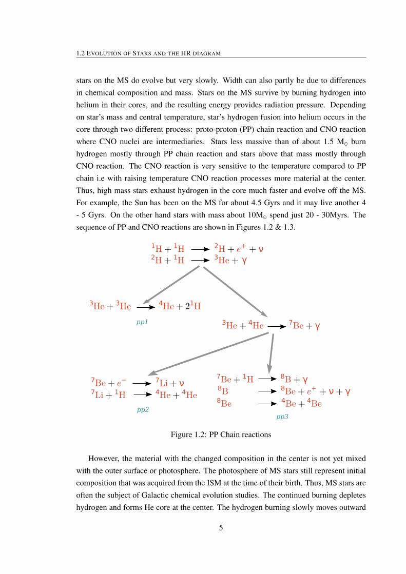
1.2 PP Chain reactions . . . . . . . . . . . . . . . . . . . . . . . . . . . . . 51.3 CNO reactions . . . . . . . . . . . . . . . . . . . . . . . . . . . . . . . . 61.4 Evolutionary tracks of 1.0 and 1.8 M computed for Z = 0.017 and Z =
0.004 are shown in blue and green lines, respectively. Base of the RGB inred broken line and RGB bump in red kinks are also shown. . . . . . . . . 7
1.5 CMD of M92 and M5 globular clusters are shown. Red giant bump ismarked in red line. . . . . . . . . . . . . . . . . . . . . . . . . . . . . . 9
1.6 Structure of AGB star. . . . . . . . . . . . . . . . . . . . . . . . . . . . . 111.7 Evolution of low, intermediate, and high mass stars. Various phases in the
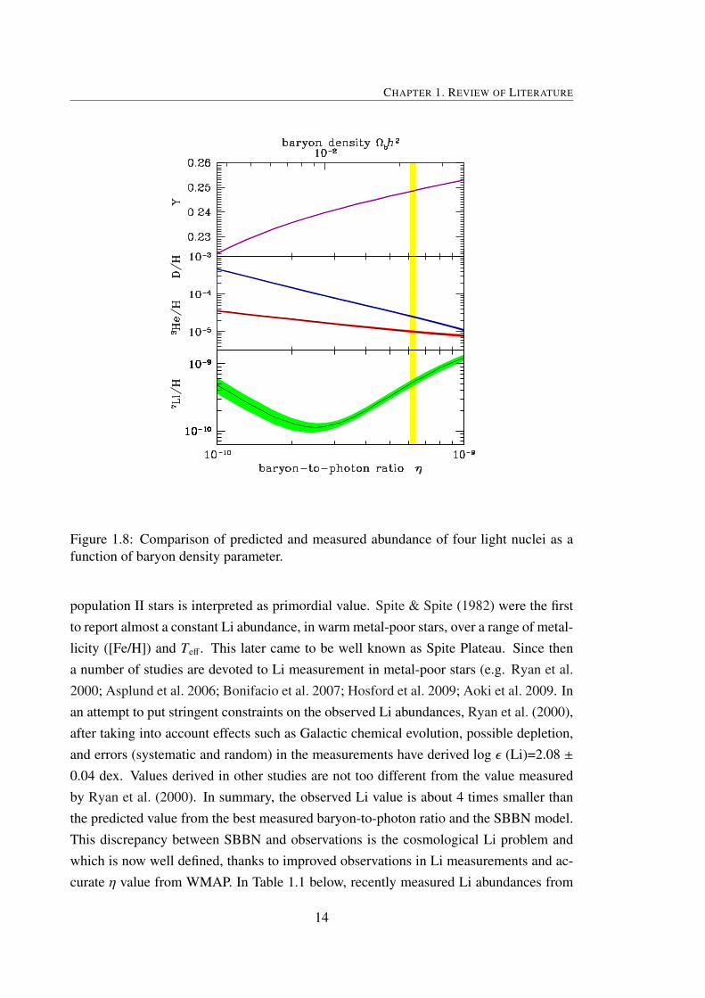
evolution are also shown. Coutesy: Herwig (2005) . . . . . . . . . . . . . 131.8 Comparison of predicted and measured abundance of four light nuclei as
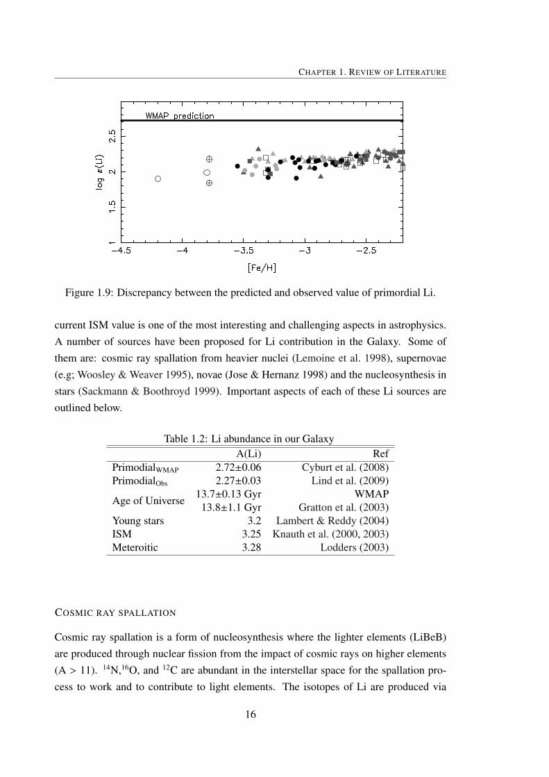
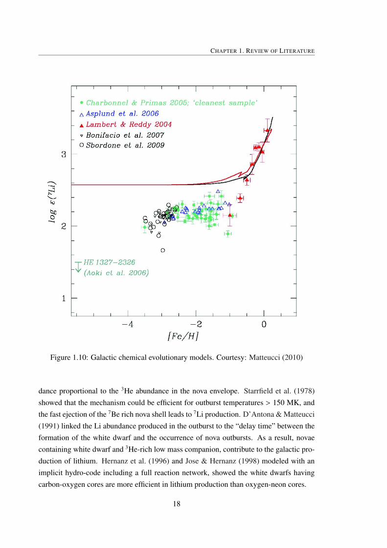
a function of baryon density parameter. . . . . . . . . . . . . . . . . . . . 141.9 Discrepancy between the predicted and observed value of primordial Li. . 161.10 Galactic chemical evolutionary models. Courtesy: Matteucci (2010) . . . 181.11 Li abundance in main sequence dwarfs. . . . . . . . . . . . . . . . . . . 21
2.1 Equivalent width of a spectral line . . . . . . . . . . . . . . . . . . . . . 39
3.1 Entire sample stars of the survey are shown in the HR diagram. Evolution-ary tracks of stars of masses from 0.8 to 3.0M and of solar metallicity,[Fe/H]=0.0, computed by Bertelli et al. (2008) are also shown. The baseof the RGB and the extent of RGB bump are marked as broken and solidred lines, respectively. The RGB clump region is shown as a thick yellowline. . . . . . . . . . . . . . . . . . . . . . . . . . . . . . . . . . . . . . 53
3.2 A sample spectra taken from HFOSC on 2-m HCT. Li line at 6707 Å,Ca lines at 6717 Å and 6572 Å, and Fe line 6592 Å are marked. Notethe strength variation of Li line relative to other lines. All other linesincluding Hα vary in strength very little or no change at all. . . . . . . . 55
3.3 A few spectra taken from UAGS on 1-m telescope at VBO. Due to slightlyhigher resolution, relatively well separated lines are seen. . . . . . . . . . 57
3.4 A few sample spectra taken from OMR spectrograph on 2.3-m VBT. Onecan easily note the effect of relatively much lower resolution (R∼2000)compared to other two spectrographs. . . . . . . . . . . . . . . . . . . . . 58
xiii

LIST OF FIGURES
3.5 Spectra of a Li-rich giant HD 233517 taken with all the three instruments.Note the effect of resolution. Spectrum that has relatively higher reso-lution has sharper and deeper lines, and also the separation between thesame lines is more. . . . . . . . . . . . . . . . . . . . . . . . . . . . . . 59
3.6 Empirical relations derived for line depth ratios and Li abundances ofknown Li-rich giants for spectra obtained from HCT . In the top panel,relation of core depth ratio of Li to Ca line ( 6572 ) and Li abundances isshown. The bottom panel shows relation for Li to Fe line (6592 Å). Thefit coefficients are provided on top of the panels. . . . . . . . . . . . . . 62
3.7 Same as Fig 3.6 but for line ratios of Li to Ca at 6717 Å. Relation derivedfrom hct spectra is shown in bottom panel. Relation derived for the spectraobtained from OMR spectrograph on 2.3-m telescope shown in top panel.The relation derived from the spectra of Known Li-rich giants observedfrom 1-m CZT is shown in middle panel. The scatter is more due to theless sample points. . . . . . . . . . . . . . . . . . . . . . . . . . . . . . 63
3.8 Li abundance of HCT samples are represented as Histogram. The dis-tribution of the sample showing Gaussian with peak Li abundance at 0.6dex. Note the Li-rich giants have occupied the tail portion. . . . . . . . . 65
3.9 Li abundance of all samples are represented as Histogram. The distribu-tion of the sample showing Gaussian with peak Li abundance at 0.7 ± 0.2dex. Note the Li-rich giants have occupied the tail portion. . . . . . . . . 66
3.10 This figure is similar to the Fig 3.1. New Li-rich giants are shown as bluecircles. The size of the circle represents the relative amount of Li. Notethe Li-rich giants have occupied the bump and clump region in the HRD. 67
4.1 Sample reduced spectra with continuum fitted of one echelle order. . . . 754.2 Mean radial velocity is determined by fitting the guassian to the distribu-
tion of radial velocity from various individual lines. . . . . . . . . . . . . 784.3 Determination of Temperature and microturbulence. Top panel shows the
iron abundance is independent of LEP and bottom panel shows the abun-dance is independent of the strength of line. . . . . . . . . . . . . . . . . 83
4.4 Ionization equilibrium of iron lines are shown in the determination ofsurface gravity of a sample star. . . . . . . . . . . . . . . . . . . . . . . . 84
4.5 The figure shows the broadening of synthetic profile matching with ob-served ones in the determination of vsin i . . . . . . . . . . . . . . . . . 86
4.6 Spectra of new Li-rich giants showing the Li line at 6707 and 6103 . . . . 874.7 Observed (filled triangles) and synthetic spectra (lines) around the Li I
lines at 6707 Å for HD77361 and HD 19745. The computed spectra forlog ε(Li) = 3.96 and 3.69 matches very well with the observed spectra. . . 88
4.8 Observed (filled triangles) and synthetic spectra (lines) around the Li Ilines at 6103 Å for HD77361 and HD 19745. The computed spectra forlog ε(Li) = 3.67 and 3.96 matches very well with the observed spectra. . . 89
xiv

LIST OF FIGURES
4.9 Synthetic spectra for four isotopic ratios 6Li/7Li = 0.0, 0.01, 0.03, and0.05 for two Li-rich K giants, HD 77361 and HD 10437. The 6Li/7Li =0.0 provides the best fit. . . . . . . . . . . . . . . . . . . . . . . . . . . 90
4.10 Non-LTE abundance corrections for 6707 Å as functions of LTE lithiumabundance for the indicated stellar parameters in the lower left cornerof each plot, to be read as Teff/ log g/[Fe/H]. S olid: Lind et al. (2009)corrections including charge transfer reactions with hydrogen as well asbound-bound transitions due to collisions with neutral hydrogen. Thecross-sections are calculated with quantum mechanics (Belyaev & Barklem2003; Croft et al. 1999). Dotted: Carlsson et al. (1994) corrections.Dashed: Takeda & Kawanomoto (2005) corrections. Dash − dotted:Pavlenko & Magazzu (1996) . . . . . . . . . . . . . . . . . . . . . . . . 92
4.11 Sample spectra show the determination of Carbon abundance from thesynthesis. . . . . . . . . . . . . . . . . . . . . . . . . . . . . . . . . . . 93
4.12 Comparison of synthetic and observed spectra for HD 77361 and the tem-plate star HD 19745 in the wavelength region of 8000 Å. Ratio of 12C/13Cis derived using the 13C14N lines at 8004.6 Å. . . . . . . . . . . . . . . . 96
4.13 Carbon, Nitrogen,and Oxygen abundances with respect to iron abundanceare plotted against Metallicity. Filled square represents HD 12203, a thickdisk giant. Open triangle represents HD 145457, planet host giant. . . . . 97
4.14 Carbon, Nitrogen,and Oxygen abundances with respect to iron abundanceare plotted against Lithium abundance. . . . . . . . . . . . . . . . . . . . 99
4.15 Carbon isotopic ratios against Li abundances . . . . . . . . . . . . . . . . 100
5.1 Detection of Strong Li line in Super Li-rich giant spectra are shown in theH-R diagram. Li and ca lines are marked . . . . . . . . . . . . . . . . . . 103
5.2 Confirmation of Li-richness in Super Li-rich giants are shown in the H-Rdiagram. Positions of 7Li and 6Li along with Fe I is marked . . . . . . . 104
5.3 Determination of 12C/13C of new super Li-rich giants are shown alongwith the Known sample,HD 19745, for comparison. . . . . . . . . . . . . 105
5.4 Super Li-rich giants are shown in the H-R diagram. Blue and magentasymbols are known and new sample giants, respectively. . . . . . . . . . 107
6.1 Li-rich and normal K giants are on the HR-diagram. Evolutionary tracksfor low mass (0.8 - 3M) stars are superposed. Blue circles representsthe Li-rich K giants and the size indicates the relative amount of lithium.Green, black, cyan, and magenta crosses represent pre-bump, red clump,bump, and post-bump giants, respectively. . . . . . . . . . . . . . . . . . 113
6.2 Li-rich and Li-normal giants are on Near IR color-color diagram. . . . . . 114
xv

LIST OF FIGURES
6.3 Location of Li-rich giants on the far infrared color-color diagram. Tri-angles are the Li-rich giants. Size of the open hexagons represents therelative amount of lithium, 1.4 ≤ A(Li) < 2.0, 2.0 ≤ A(Li) < 2.5, 2.5 ≤A(Li) < 3.3, and A(Li) ≥ 3.3, respectively. Red square is the Arcturus, atypical K giant with A(Li) < 0.0 . Black color indicates the upper limitsof fluxes at 25µ and 60µ. Blue color is for the upper limit flux at 60µ. Redcolor is for the high and moderate quality fluxes at 12, 25, and 60µ . . . . 117
6.4 Li-rich and normal giants with only good quality of data are presented.Filled triangles are the Li-rich K giants. Open symbols are normal gi-ants. Triangles, squares, pentagons and hexagons represent pre-bump,bump,clump, and postbump, respectively . . . . . . . . . . . . . . . . . . 118
6.5 A plot of dust temperature (Td) against the dust opacity index (α) for ob-served flux ratios of HDE 233517. Blue and pink colors represent thecombination for (F12/F25) and (F25/F60), respectively. The intersectionpoint represents the dust temperature and α for the dust shell (Td = 219and α = -1.73). . . . . . . . . . . . . . . . . . . . . . . . . . . . . . . . . 119
6.6 Combinations of dust temperature (Td) and dust opacity index (α) for ob-served flux ratios of Arcturus. Blue and pink colors represent the combi-nations for (F12/F25) and (F25/F60), respectively. Both curves are diverging. 121
6.7 Sample spectra showing the Hα emission in blue wing. It also show thesatellite lines of Na D1 and D2. . . . . . . . . . . . . . . . . . . . . . . . 122
6.8 Spectral energy distribution of observed fluxes superposed with the theo-retical fluxes modeled from DUSTY. . . . . . . . . . . . . . . . . . . . . 124
6.9 Li abundance against mass-loss rates of Li-rich K giants are plotted inleft panel. Li abundance against dust temperatures of Li-rich K giants areplotted in left panel. Li abundance was derived from the high resolutionspectra. Mass-loss rates and dust temperatures are obtained from this work.127
6.10 Sample giants and dust shell evolutionary models are on color-color dia-gram. Li-rich giants with various quality data are presented on left panel.On the right panel, Li-rich and normal giants with only good quality ofdata are presented. Different colors, magenta, green, cyan and blue rep-resents the loops of the evolution of a dust shell with mass-loss rates,1×10−10, 1×10⁻⁹, 5×10⁻⁹, and 3×10⁻⁸, respectively. Four varieties oflines in each color indicate the different photospheric temperatures andradius, Te f f = 5000 K, R = 20 R, Te f f = 4000 K, R = 20 R, Te f f = 5000K, R = 10 R, Te f f = 4000 K, R = 10 R of the dust shell hosting stars,radially outwards, respectively. . . . . . . . . . . . . . . . . . . . . . . . 129
7.1 Distribution of samples from our survey and Brown et al.’s survey. Lumi-nosities are in left panel and Temperatures are in right panel. . . . . . . . 138
xvi
LIST OF FIGURES
7.2 Sample stars of our survey in blue symbols and from B89 survey in greensymbols are shown in the HR diagram. Evolutionary tracks of stars ofmasses from 0.8 to 3.0M and of solar metallicity, [Fe/H]=0.0, computedby Bertelli et al. (2008) are also shown. The base of the RGB and the ex-tent of RGB bump are marked as broken and solid red lines, respectively.The RGB clump region is shown as a thick yellow line. . . . . . . . . . . 139
7.3 Same as Figure 7.2. New Li-rich giants are in blue symbols and greensymbols are from Brown and magenta symbols are other known Li-richgiants. . . . . . . . . . . . . . . . . . . . . . . . . . . . . . . . . . . . . 141
xvii

LIST OF TABLES
1.1 Primordial Lithium abundance . . . . . . . . . . . . . . . . . . . . . . . 151.2 Li abundance in our Galaxy . . . . . . . . . . . . . . . . . . . . . . . . 161.3 Contributions from various sources in Galactic evolutionary models. . . . 19
3.1 Basic data of a few stars in the sample survey. . . . . . . . . . . . . . . . 513.2 Journal of Observations . . . . . . . . . . . . . . . . . . . . . . . . . . . 543.3 Derived line depth ratios and Li abundances for K giants that are used in
deriving relations. . . . . . . . . . . . . . . . . . . . . . . . . . . . . . 603.4 Measurements of line ratios and derived Li abundance of sample stars . . 643.5 Statistical analysis of Sample stars . . . . . . . . . . . . . . . . . . . . . 643.6 Derived parameters of new Li-rich giants . . . . . . . . . . . . . . . . . 66
4.1 Absolute magnitude and Luminosity of new Li-rich giants from basic dataavailable in Hipparcos catalog . . . . . . . . . . . . . . . . . . . . . . . 72
4.2 Journal of Observations . . . . . . . . . . . . . . . . . . . . . . . . . . . 734.3 Derived temperatures from various photometric colors. . . . . . . . . . . 764.4 Derived surface gravities from astrometry and photometry . . . . . . . . 774.5 Measurement of line shifts for few selected lines to derive radial velocity. 794.6 Derived radial velocities along with literature values . . . . . . . . . . . 804.7 Space velocities, orbital parameters, and probability distribution in Galaxy
. . . . . . . . . . . . . . . . . . . . . . . . . . . . . . . . . . . . . . . . 814.8 Atomic data of selected lines and their equivalent widths for few sample
Li-rich giants . . . . . . . . . . . . . . . . . . . . . . . . . . . . . . . . 824.9 Derived spectroscopic atmospheric parameters from high resolution spec-
tra . . . . . . . . . . . . . . . . . . . . . . . . . . . . . . . . . . . . . . 854.10 Derived projected rotational velocities . . . . . . . . . . . . . . . . . . . 854.11 Derived Lithium abundance . . . . . . . . . . . . . . . . . . . . . . . . 914.12 CNO abundances and 12C/13C ratios . . . . . . . . . . . . . . . . . . . . 95
5.1 Values of stellar parameters (Metallicity, Teff , Mass, luminosity) and thesurface abundances values of log ε(Li) and carbon isotopic ratios of superLi-rich K giants. . . . . . . . . . . . . . . . . . . . . . . . . . . . . . . 106
6.1 IRAS fluxes of Li-rich giants from IPAC 1986 . . . . . . . . . . . . . . . 1166.2 Dust Temperature and dust opacity index of Li-rich and Li-normal K gi-
ants . . . . . . . . . . . . . . . . . . . . . . . . . . . . . . . . . . . . . 1206.3 Mass-loss rates derived from Reimer’s law . . . . . . . . . . . . . . . . 125
xix

LIST OF TABLES
6.4 Photospheric and dust parameters of Li-rich K giants. . . . . . . . . . . . 1266.5 Dust parameters and evolutionary timescales for different photospheric
parameters . . . . . . . . . . . . . . . . . . . . . . . . . . . . . . . . . 1286.6 Evolutionary timescales from bump to clump . . . . . . . . . . . . . . . 1316.7 Circumstellar shell evoltuionary models . . . . . . . . . . . . . . . . . . 132
xx

CHAPTER 1
REVIEW OF LITERATURE
1.1 GENERAL INTRODUCTION
The splendor and grandeur of the night sky always fascinated the humankind. The artfulpatterns of stars and planets, and their passage across the night sky inspired many, sincethe beginning of human race, to ponder over the dazzling, and yet a systematic and largelya periodic phenomenon. The periodic appearance and disappearance of celestial objectshelped societies and cultures to define time, track seasons, harvest crops, invent naviga-tional tools, and devise calendars for their day-to-day activities. Astronomy, therefore,is considered as the oldest branch of natural sciences. The systematic observations andthe human quest to understand the great importance of the physical universe has led toa remarkable spectrum of inventions and discoveries. From years of careful watching ofthe night sky with naked eye, centuries before the dawn of the telescope, our ancestorsobserved that some stars move in the night sky with respect to the others. The movingstars were called planets. This led to the idea of solar system where the Sun, Earth, andother planets are different from rest of the stars in the sky. In around 140AD, Greek as-tronomer Ptolemy developed the theory of geocentric universe where everything else inthe universe goes around the Earth. About fourteen hundred years later, the geocentrictheory was discarded with much better and accurate observational data on planetary mo-tions accumulated by Tycho Brahe, and the data helped Jonathan Kepler to formulate thefamous laws of planetary motions. These observations gave foundation to Isaac Newtonto formulate the famous universal theory of gravitation.
With the advent of the telescope in early 1600AD, the new era began in astronomy.Galileo Galilee was the first to use the telescope in 1609AD and made landmark discov-eries such as four moons revolving around the planet Jupiter which shattered the myth
1
CHAPTER 1. REVIEW OF LITERATURE
that our earth is unique in the universe. This also gave an idea that there is much moreto discover in the universe with better and larger aperture telescopes. A race to makebigger and better telescopes began. With it came the rapid change the way the universewas viewed.
In the early part of 1900s, Edwin Hubble using the observations of galaxies with the2.5m Hooker telescope, Mount Wilson Observatory, made a remarkable discovery of theexpansion of the universe. Farther the galaxies faster they appeared to recede from us.The immediate implication of Hubble’s discovery was that our universe was much morecompact in the past and must have had beginning in time. This, later became an activearea of research, the big bang cosmology. The big bang interpretation was supported bythe discovery of astonishingly smooth microwave background radiation in the universe.In the last 100 years, astronomers with the aid of sophisticated telescopes and instrumentsmade stupendous progress in understanding many aspects of our observable universe. Thefindings include; development of stellar evolution theory, understanding of synthesis ofelements in stars, discovery of dark matter, evidence of the accelerated expansion of theuniverse probably due to an unknown form of energy known as dark energy, finding ofexo-planetary systems etc.
Studies of the stars and stellar systems played important roles in our understandingof the universe and its evolution. Stars are the building blocks of the galaxies which inturn make-up the universe. Detailed understanding of the stars, their internal structure,evolution, and chemical composition is essential to decipher the birth and the evolutionarysequence of the galaxies. Much of current understanding of stellar structure and evolutioncould easily be traced back to early and mid 1900s research of eminent astrophysicists likeA. Emden, James Jeans, A.S. Eddington, S. Chandrasekhar, M. Schwarzschild, Ico Ibenand many others. Though the basic stellar physics is on sound foundations, there arestill many outstanding issues which need to be probed for better clarity. For example,still there is no clear consensus on how exactly stars form out of collapsing clouds andtheir early evolution. Also, gaps exist in our understanding of different phases of stellarevolution: Main Sequence (MS), Red Giant Branch (RGB), Horizontal Branch (HB),Asymptotic Giant Branch (AGB), post-AGB, Planetary Nebulae (PNe), and the transitionto the final phase such as white dwarf, neutron stars or black holes. Since the thesis isconcerned about a particular phase of stellar evolution (RGB phase), a brief descriptionof evolution of the stars at various phases of their life is provided.
2

1.2 EVOLUTION OF STARS AND THE HR DIAGRAM
1.2 EVOLUTION OF STARS AND THE HR DIAGRAM
Star’s evolution is mainly dictated by its initial mass. Stars with higher mass will evolvemuch faster compared to lower mass stars. The evolution of a star is characterized by itschange in effective temperature (Teff), surface gravity (g), and chemical composition. Inother words, as the star evolves it continuously changes its color and brightness whichare generally represented by (B-V) and luminosity (log L/L), respectively. Dependingon their initial mass, evolution of stars are classified into three mass categories: low-mass(up to about 2M), intermediate mass (2 - 10M) and massive stars evolution.
Figure 1.1: Evolution of 2 M star is shown in H-R diagram. Various phases are alsohighlighted. Courtesy: Herwig (2005)
The changes in the star’s life are conveniently shown in a diagram of luminosity ver-sus color (or Teff) which is the famous Hertzsprung-Russel diagram or HRD after the twofamous astronomers Ejnar Hertzsprung and Henry Norris Russel who independently re-alized the usefulness of such a diagram. The main stages of star’s evolution for a 2M
star is illustrated in Figure 1.1. Below we describe each of these stages in more detail.Emphasis is given to low- and intermediate mass star’s evolution.
3

CHAPTER 1. REVIEW OF LITERATURE
1.2.1 PRE-MAIN SEQUENCE PHASE
Star’s evolution from its birth in the molecular clouds to the main sequence is calledas pre-main sequence phase. In general, star formation or the cloud collapse processbegins, as suggested by Jeans (1928), with small density fluctuations which steadily growby gravity. When the fluctuations exceed some critical intensity, cloud becomes gravitydominated, the collapse begins, a process known as gravitational instability. Thus, thegravity is the fundamental driving force in the star formation process. Star formationcan occur only where the gas becomes dense enough for its self-gravity to over comethe effects such as thermal pressure, turbulence, magnetic fields etc. This sets a limiton a minimum mass, called Jean’s mass, that a cloud must have to collapse under itsgravity. Thus, an isothermal cloud of certain mass and temperature of the order of 6-10K begins to collapse under its own gravity. As the collapse continues central densityincreases which increases optical depth. Hence center becomes opaque and as a resultradiative cooling becomes unimportant. The cloud becomes adiabatic leading to a rapidraise in temperatures at the center. Thermal pressure builds up at the center halting furthercollapse. However, the core keeps growing in mass by accreting material that is leftbehind during the collapse. At about 2000 K, hydrogen molecules begin to dissociatemaking the core unstable again. Further rapid collapse ensures a complete ionisation ofH at the center and a complete halt to collapse, a protostar is formed at the center withhydrostatic equilibrium. The accreting protostar becomes a normal pre-main sequencestar, which by then has acquired nearly all of its mass by accretion from the envelop.
Further, protostar becomes hotter and increases its brightness while shrinking in size.As the protostar evolves temperature of the core reaches to burn hydrogen through nu-clear fusion. Finally, stars are in hydrostatic equilibrium, outward radiation pressure isbalanced by the inward gravity force, settle on the Zero-age main sequence (ZAMS). Inour Galaxy, observations show that much of the star formation occurs in the spiral armsand also in the central regions. T-Tauri stars are the youngest (about 1 Myr) visible stars,and these are pre-main sequence stars that have not yet become hot enough at their centersto burn hydrogen and begin the main-sequence phase of evolution.
1.2.2 MAIN SEQUENCE
After reaching hydrostatic equilibrium protostars arrive at the most stable and long lastingphase of their evolution, the main sequence phase or MS. Obviously, the MS phase in theHRD, as shown in Figure 1.1, is the most populated, and the width of the MS suggests
4
1.2 EVOLUTION OF STARS AND THE HR DIAGRAM
stars on the MS do evolve but very slowly. Width can also partly be due to differencesin chemical composition and mass. Stars on the MS survive by burning hydrogen intohelium in their cores, and the resulting energy provides radiation pressure. Dependingon star’s mass and central temperature, star’s hydrogen fusion into helium occurs in thecore through two different process: proto-proton (PP) chain reaction and CNO reactionwhere CNO nuclei are intermediaries. Stars less massive than of about 1.5 M burnhydrogen mostly through PP chain reaction and stars above that mass mostly throughCNO reaction. The CNO reaction is very sensitive to the temperature compared to PPchain i.e with raising temperature CNO reaction processes more material at the center.Thus, high mass stars exhaust hydrogen in the core much faster and evolve off the MS.For example, the Sun has been on the MS for about 4.5 Gyrs and it may live another 4- 5 Gyrs. On the other hand stars with mass about 10M spend just 20 - 30Myrs. Thesequence of PP and CNO reactions are shown in Figures 1.2 & 1.3.
1H+
1H
2H+ e
++ ν
2H+
1H
3He + γ
3He +
3He
4He + 2
1H
3He +
4He
7Be + γ
7Be + e
− 7Li + ν
7Li +
1H
4He +
4He
7Be +
1H
8B+ γ
8B
8Be + e
++ ν+ γ
8Be
4Be +
4Be
pp1
pp2pp3
Figure 1.2: PP Chain reactions
However, the material with the changed composition in the center is not yet mixedwith the outer surface or photosphere. The photosphere of MS stars still represent initialcomposition that was acquired from the ISM at the time of their birth. Thus, MS stars areoften the subject of Galactic chemical evolution studies. The continued burning depleteshydrogen and forms He core at the center. The hydrogen burning slowly moves outward
5

CHAPTER 1. REVIEW OF LITERATURE
forming a ring like structure (H-shell) around the He ash core. Once the entire H is burntthe structural changes in the interior ensure stars evolve off the MS towards right (coolerTeff) in the HRD. Stars grow in size, become cooler and brighter, a beginning of a newphase in their evolution.
(p,γ)
(p,γ) (p,α)
(β+ ) (β
+)
(p,γ
)
(p,α)
(p,γ
)
(p,γ)
(β+)
13C
13N
12C
15N16O
17F
17O
14N
15O
Figure 1.3: CNO reactions
1.2.3 POST-MAIN SEQUENCE
The post-main sequence (Post-MS) evolution of a stars depends on their initial masswhich controls the central temperature. The post-MS evolution of the low- and intermedi-ate stars has a few significant phases which play greater roles in the chemical enrichmenthistory of the Galaxy. These are: The red giant branch (RGB), Horizontal branch (HB),Asymptotic giant branch (AGB), post-AGB and Planetary Nebulae (PNe). Of course, de-pending on the initial stellar mass stars end their lives either as white dwarfs (low- andintermediate mass stars), neutron stars or black holes (massive stars). Here, we brieflydescribe salient features of each of these phases.
RED GIANT BRANCH
As the He-core contracts star evolves off the MS and hydrogen starts to burn in a shell.The increased energy production in the interior results in star’s overall expansion, and alsorapid reduction in surface temperature. By the time the star reaches the base of RGB the
6

1.2 EVOLUTION OF STARS AND THE HR DIAGRAM
convection reaches its maximum extension in mass (Salaris et al. 2002) and extends all theway to the hydrogen burning shell. For the first time, the processed interior material getsexposed to the surface. The mixing of interior material with the outer surface will alter thephotospheric chemical composition. This phenomenon in RGB stars is called the “firstdredge-up”. The first dredge-up brings up the material with reduced 12C, increased 14N,3He and 13C. Also, a significant reduction in Li abundance is observed. The Li evolutionin RGB stars seems to be a complex phenomenon. A more detailed description of Li inRGB stars is provided later in this chapter.
5500 5000 4500 4000
0.5
1
1.5
2
2.5
Z= 0.008
Z= 0.017
Figure 1.4: Evolutionary tracks of 1.0 and 1.8 M computed for Z = 0.017 and Z = 0.004are shown in blue and green lines, respectively. Base of the RGB in red broken line andRGB bump in red kinks are also shown.
In the case of low mass (≤ 2.25 M) RGB stars, core is a degenerate He gas (Iben1968; Bertelli et al. 2008). As the H-burning shell continues to deposit He, the densityof the core increases and hence the temperature. Stars move-up on the RGB rapidly withlarge increase in luminosity. As they moves-up the convection zone begins to retreat fromthe deepest point of penetration leaving H-discontinuity between H-burning shell andthe base of convective zone. At this point as models suggest (Iben 1968) the H-burningshell moves upward until it encounters the H-discontinuity that was created at the time
7

CHAPTER 1. REVIEW OF LITERATURE
of first-dredge up. At the encounter, H-burning shell is provided with more H fuel whichtemporarily cools the central temperature leading to reduced luminosity. This creates akink on the RGB known as RGB luminosity bump (see Figure 1.4). The bump seemsto happen for only low mass stars which have degenerate He-core. The bump occurs,depending on mass, in the luminosity range logL/L = 1.3 - 2.4 (Bertelli et al. 2008).This internal mechanism in the evolution of RGB effects its evolution. The slowing downof evolution at the bump is manifested over density of stars at the RGB bump region.Observations of open and globular clusters (Di Cecco et al. 2010 and references there in), dwarf spheroidal galaxies (Bellazzini et al. 2005), LMC and SMC, show (see Figure 1.5)evidence of such luminosity bump.
After a while equilibrium is established in the interior, and the stars starts againclimbing-up towards the tip of RGB (TRGB). The continued depositing of He from H-burning increases the core density which raises its temperature sharply. The thermal runaway occurs in the He degenerate core, due to the continued rise in temperature resultingin He-flash. He-flash lifts the degeneracy and the core expands and outer layers shrink insize. Stars climb down in luminosity with slight increase in Te f f . As shown in Figure 1.5,stars post-He flash, probably, end up as HB stars. Stars in the horizontal branch burn Hein the core under non-degenerate conditions and H-burning in the shell. A new phaseof evolution has begun which is also known as He-main sequence for He-burning at thecenter.
HORIZONTAL BRANCH
Stars on horizontal branch (HB) are analogues to the main sequence stars. The differ-ence being in HB stars are He-core with H-burning in a shell. Much earlier Hoyle &Schwarzschild (1955) identified that the HB stars are nothing but the stars evolved fromthe RGB. Evolution from the tip of the RGB, after He-flash, to the stable HB is quiterapid and is not well understood. All the low and intermediate mass stars evolve to HB.Stars on the HB stay for a longer period with almost same luminosity but with a rangeof temperatures. Evolutionary time scales on HB are subject to their initial mass andalso composition. Stars that are massive enough would undergo He fusion through 3α-reaction. The by-product is carbon which gets deposited at center. As He-burns, corecontracts and stars make structural adjustments to maintain hydrostatic equilibrium. Asa result stars shrink in radius which ensures almost constant luminosity with rise in tem-perature.
Once the He burning gets over at the center, and moves to shell He-burning HB stars
8

1.2 EVOLUTION OF STARS AND THE HR DIAGRAM
Figure 1.5: CMD of M92 and M5 globular clusters are shown. Red giant bump is markedin red line.
begin to ascend once again towards higher luminosity. The second ascent phase is knownas asymptotic giant branch. All the HB stars may not ascend second time. Low mass starsdepending on their chemical composition or heavy mass loss during the RGB end up ashot extreme HB stars (e.g. Mohler 2004).
9

CHAPTER 1. REVIEW OF LITERATURE
ASYMPTOTIC GIANT BRANCH
All low and intermediate stars of about 1-10M experience the AGB phase. AGB starsare the final evolutionary stage of low- and intermediate-mass stars driven by nuclearburning. This phase of evolution is characterized by nuclear burning of hydrogen andhelium in thin shells on top of the electron-degenerate core of carbon and oxygen (SeeFigure 1.6). In the case of the most massive (∼ 8 - 10 M) AGB stars core is of oxygen,neon, and magnesium. AGB phase is characterized by series of thermal pulses as a resultof competing energy sources of He- and H- burning shells creating deep convective en-velope. AGB stars expand significantly and they are as large as R∼100R. As a result oflarge size and thermal pulses AGB stars lose mass heavily. It is estimated that about 70%of the dust in the Galaxy is due to the AGB stars. Also, they provide a rich environmentfor nuclear production. The primary C- and N-, and much of the s-process elements (Y,Ba, Nd, etc.) in the universe are mainly produced in the interiors of the AGB stars. Thenew element rich material is brought up to the photosphere as a result of deep convectivezone and recurring thermal pulses, phenomenon known as 3rd dredge-up. Depending onthe initial mass, AGB stars either become C-rich or O or N-rich stars. Stars with initialmass less than about 4 M, become C-rich (C/O ≥ 1) as fresh C, result of He-triple alphareaction, is pumped-up to the surface. The more massive AGB stars (above 4 M) be-come O-rich (or N-rich stars) due to hot bottom burning (HBB). In more massive stars itis found that nucleosythesis occurs in the convective zone where the CNO reaction con-verts much of the primary carbon into nitrogen. This would reduce amount of carbon inthe envelope and hence star becomes O-rich (C/O < 1) or highly N enhanced AGB star.
Due to heavy mass-loss towards the tip of the AGB, stars are obscured by heavydust and invisible in optical wavelengths. These stars are mostly studied in IR and mil-limeter observations. Stars in this phase are also called OH/IR stars. The continuedmass loss depletes mass of the H-envelope, and when a star reaches some critical value(about 10−3Myr−1 ), it ends the AGB phase and moves left, in the HR diagram, towardsplanetary nebulae (PNe) phase. There are quite a good number of reviews on AGB starevolution in the literature (e.g; Iben & Renzini 1983; Herwig 2005).
POST-AGB EVOLUTION
Evolutionary phase of stars between AGB and PNe is known as post-AGB or some timesproto-planetary nebula (pPNe) phase. Time scales of post-AGB phase are relatively verysmall of the order of a few tens of thousand years. All the low- and intermediate- mass
10

1.2 EVOLUTION OF STARS AND THE HR DIAGRAM
He intersh
ellConv
ective En
velope
Initial composition
-modified by first
dredge-up
He burning shell
H burning shell
12C4He
1H 4He
4He(14N)
Figure 1.6: Structure of AGB star.
stars go through this phase. Post-AGB stars evolve from right to left (AGB to PNe) withconstant luminosity and increasing surface temperature. Identification of post-AGB starsis difficult as they evolve much faster and also they appear like population I supergiantsin the visible wavelengths. Number of post-AGB stars were discovered following theIRAS mission in 1983. Post-AGB stars show characteristic of far-IR colours with dusttemperatures ranging between 100 - 300 K. The surface abundances of post-AGB starsreflect the nucleosynthesis and dredge-up process that occurred during the star’s AGBevolution. The dust envelope that was created during the AGB phase slowly moves awayfrom the central star. In slightly massive stars surface temperature rises fast enough toionize the dust which appears as nebula. Stars enter into PNe phase. In the case oflow mass stars, evolution is slow and the dust envelope dissipates by the time surfacetemperature rises enough to ionize the dust.
PLANETARY NEBULAE
PNe harbour a very hot compact star at their center and surrounded by dense torus ofmaterial presumably ejected earlier in the life of the AGB star. The morphologies of PNeare found to be complicated, and are categorised into three major types: round, elliptical,and bipolar. Normally, all PNes show reflection symmetry about their major and minor
11

CHAPTER 1. REVIEW OF LITERATURE
axes (e.g. HST image of Cat’s Eye Nebulae (Harrington & Borkowski 1994) given inFig (ref), showed the shape of the PNe and jet-like structures). PNe’s occupy the top leftcorner in the HRD, shown in Figure 1.1 The central stars of PNe are classified into twotypes: hydrogen normal and hydrogen deficient. (e.g R Coronae Boriolis star). The originof H-deficiency in these stars are not well understood. There are few explanations existingin the literature: e.g. Born-again star scenario, in which a postAGB star (or WD) reigniteshelium-shell burning and transforms the star back into an AGB star (See the green star inFigure 1.1). The temperatures of the central stars are in the order of 104 which ionizesthe nebular material and makes it visible. The abundances of nebular material is rich withheavier elements that have been synthesized inside the stars during their early evolution.The nebula expands to a great extent and merges into ISM, and the fully exposed coreof the central star enters into white dwarf phase. In this way stars add heavier elementsto its intital material and return back to ISM. Hence PNe play a crucial role in chemicalevolution of the Galaxy. The intrinsic brightness of all PNe’s are similar hence these arepotential standard candles for the measurements of extragalactic distances.
WHITE DWARFS
White dwarf is the end state of stars (< 4M ) which is highly densed object supportedby degenrate-electron pressure. White dwarfs are very hot with temperatures of the order105. Since there is no source of energy, it radiates all the energy and cools down. These arecalled cold black dwarfs. Similarly, the stars with higher masses (> 4 M) evolve throughvarious phases and ends their lives as neutron stars or blackholes (See Figure 1.7)
1.3 LITHIUM IN THE UNIVERSE
Li is one of the light elements with atomic number 3. It is found in two flavors: 7Liand 6Li. It is fragile, and gets destroyed at about 2-2.5 × 10⁶K, such temperatures arecommon in stellar interiors. Hence its evolution is found to be a complex phenomenon. Itis important to understand its evolution in the universe, in general, and in our Galaxy andin stars, in particular. Its study would enhance our understanding of the nucleosynthesis atthe time of big bang and its evolution since then. In the case of stars, Li study would helpto better constrain theoretical models dealing with the internal structure and dredge-upprocess. Thus, Li is considered as a crucial element to validate Big Bang nucleosynthesismodels and an important diagnostic of standard and non-standard stellar evolutionarytheories. Though our study is primarily focused on Li in RGB stars, we thought, it would
12

1.3 LITHIUM IN THE UNIVERSE
Figure 1.7: Evolution of low, intermediate, and high mass stars. Various phases in theevolution are also shown. Coutesy: Herwig (2005)
be relevant to provide an overview of Li content in various systems: old-metal poor stars(primordial value), ISM, and stars in the current epoch.
1.3.1 PRIMORDIAL LITHIUM
What is the primordial Lithium abundance? This question prevailed for quite some timeand was debated in numerous studies. Yet, the answer seems to be not in sight. Thediscrepancy between the predictions made by big bang nucleosynthesis (BBN) modelsand the Li measurements made in metal-poor stars is too significant to be reconciled with.The main isotope of lithium (7Li) along with other light elements hydrogen, Deuterium(D), 3He, and He are known to have been produced during the big bang nucleosynthesis.The standard big bang nucleosynthesis (SBBN) models predict abundances of these fournuclei if the baryon-to-photon ratio (η) or a cosmological baryon density (Ωbh2), a freeparameter in SBBN, is fixed. The η value can be measured either by measuring the relativeabundances of any two of the four nuclei or by measuring microwave background (CMB)with experiments such as WMAP (e.g; Dunkley et al. 2009). The current best valuesfor (Ωbh2) are 0.02273 ± 0.00062 (Dunkley et al. 2009) and 0.0214 ± 0.0020 (Kirkmanet al. 2003) measured by five years WMAP data and by using D/H ratios measured inQSO absorption systems, respectively (see Figure 1.8) . These values correspond SBBNprediction of 7Li abundance of log ε (Li) =2.72 ± 0.06 dex (Cyburt et al. 2008).
In the case of observations, Li abundance derived in hot (more than about 5800 K)
13
CHAPTER 1. REVIEW OF LITERATURE
Figure 1.8: Comparison of predicted and measured abundance of four light nuclei as afunction of baryon density parameter.
population II stars is interpreted as primordial value. Spite & Spite (1982) were the firstto report almost a constant Li abundance, in warm metal-poor stars, over a range of metal-licity ([Fe/H]) and Teff . This later came to be well known as Spite Plateau. Since thena number of studies are devoted to Li measurement in metal-poor stars (e.g. Ryan et al.2000; Asplund et al. 2006; Bonifacio et al. 2007; Hosford et al. 2009; Aoki et al. 2009. Inan attempt to put stringent constraints on the observed Li abundances, Ryan et al. (2000),after taking into account effects such as Galactic chemical evolution, possible depletion,and errors (systematic and random) in the measurements have derived log ε (Li)=2.08 ±0.04 dex. Values derived in other studies are not too different from the value measuredby Ryan et al. (2000). In summary, the observed Li value is about 4 times smaller thanthe predicted value from the best measured baryon-to-photon ratio and the SBBN model.This discrepancy between SBBN and observations is the cosmological Li problem andwhich is now well defined, thanks to improved observations in Li measurements and ac-curate η value from WMAP. In Table 1.1 below, recently measured Li abundances from
14

1.3 LITHIUM IN THE UNIVERSE
Pop II stars and the values computed from SBBN are given, where logε(Li) = log(Li/H)+ 12.
Table 1.1: Primordial Lithium abundanceSource A(Li)a Ref
Predicted SBBN+WMAP 2.72±0.06 Cyburt et al. (2008)
Observed
Spite Plateau 2.05±0.15 Spite & Spite (1982)
Halo stars2.08±0.04 Ryan et al. (2000)2.10±0.09 Bonifacio et al. (2007)2.18±0.04 Hosford et al. (2009)
Globular clusters2.34±0.06 Bonifacio et al. (2002)2.24±0.05 Korn et al. (2006)
Average Li 2.27±0.03 Lind et al. (2009)aA(Li) = log ε(Li) = log(Li/H) + 12
As the problem is well defined, studies turned to look for other reasons for the dis-crepancy. Assuming that SBBN value and also the measured Li abundance in stars arecorrect one would make a suggestion that the primordial Li has been severely destroyedin the Galaxy before the formation of old metal-poor stars by astration of matter in mas-sive Pop III stars (Piau et al. 2006). Also, it could be that the original Li in Pop II starsmight have been depleted due to internal processes such as atomic diffusion and mixing(Richard et al. 2005; Korn et al. 2006; Lind et al. 2009). Also, one can’t rule out thepossibilities of uncertainties in the input parameters of SBBN. Some of these may benuclear reaction rates and cross sections (Cyburt et al. 2008). However, to the presentknowledge, the discrepancy between the predictions and observations of primordial Li,shown in Figure 1.9, is a challenge that need to be tackled.
1.3.2 GALACTIC LITHIUM
Young open clusters and the the main sequence pop I stars have been found to have a max-imum Li abundance of log ε (Li) = 3.2 dex. This is in good agreement with the measuredLi value in different molecular clouds which represents ISM value (See Table 1.2). Fromthis, one can safely draw a conclusion that the maximum Li abundance found in mainsequence (e.g; Lambert & Reddy 2004) stars and in ISM is the value that represents Liin current epoch or the cosmic Li abundance. The current Li abundance is about an orderof magnitude more than the observed Li abundance, believed to be a primordial value, inpop II dwarfs. Understanding of enrichment history of Li from Spite plateau value to the
15
CHAPTER 1. REVIEW OF LITERATURE
Figure 1.9: Discrepancy between the predicted and observed value of primordial Li.
current ISM value is one of the most interesting and challenging aspects in astrophysics.A number of sources have been proposed for Li contribution in the Galaxy. Some ofthem are: cosmic ray spallation from heavier nuclei (Lemoine et al. 1998), supernovae(e.g; Woosley & Weaver 1995), novae (Jose & Hernanz 1998) and the nucleosynthesis instars (Sackmann & Boothroyd 1999). Important aspects of each of these Li sources areoutlined below.
Table 1.2: Li abundance in our GalaxyA(Li) Ref
PrimodialWMAP 2.72±0.06 Cyburt et al. (2008)PrimodialObs 2.27±0.03 Lind et al. (2009)
Age of Universe13.7±0.13 Gyr WMAP13.8±1.1 Gyr Gratton et al. (2003)
Young stars 3.2 Lambert & Reddy (2004)ISM 3.25 Knauth et al. (2000, 2003)Meteroitic 3.28 Lodders (2003)
COSMIC RAY SPALLATION
Cosmic ray spallation is a form of nucleosynthesis where the lighter elements (LiBeB)are produced through nuclear fission from the impact of cosmic rays on higher elements(A > 11). 14N,16O, and 12C are abundant in the interstellar space for the spallation pro-cess to work and to contribute to light elements. The isotopes of Li are produced via
16
1.3 LITHIUM IN THE UNIVERSE
spallation reactions (Reeves 1970; Meneguzzi et al. 1971) when Galactic Cosmic Rays(GCR), mainly protons, interact with C,N, and O nuclei in the interstellar medium. It isbelieved that the amount of 6Li present in the universe is entirely produced through cos-mic ray spallation, whereas only small fraction of 7Li is understood to be produced. Theevidence for 7Li production in the GCR has been inferred using the Be and B abundancesthat are seen in Pop II stars (Olive & Schramm 1992). Be and B abundances do not showplateau unlike 7Li suggesting B and B are mainly from GCR and 7Li must be from bigbang. Lemoine et al. (1998) calculated the amount of 7Li produced by GCR. However,the observational evidence of 7Li production through GCR process is not well tested. Thedetection of a significantly high amount of 6Li (6Li/7Li ≈ 0.05) in some of the Pop II starsis one of the evidences that Li gets produced in the GCR through α-α fusion reactions(Smith et al. 1993; Asplund et al. 2006).
SUPERNOVAE NUCLEOSYNTHESIS
The core of massive stars collapses to form a neutron star and explode as supernovae.Most of the gravitational energy released at the explosion is carried away by neutrinos (∼1058) emitted from the central remnant. Although cross section of neutrino-nucleus reac-tions are very small, such a large number of neutrinos enable to contribute the increasein the yields of some species of light nuclei. This process is called ν-nucelosynthesis(Woosley et al. 1990). During the formation of the neutron star in the pre-explosionphase, SNe II II can produce 7Li in the He-shell by excitation of 4He by µ- and τ- neu-trinos followed by de-excitation with emission of a proton or neutron, via 4He(ν,ν
′
n)3He,which in turn reacts with α particle and forms 7Li via Be-transport mechanism.Woosley &Weaver (1995) calculated the detailed 7Li yields from SNe II as functions of initial stellarmetallicity. Unfortunately, the theoretical suggestion of possible Li production throughν-process is not confirmed by observations.
NOVAE SYNTHESIS
Classical novae could also in principle be 7Li producers. Della Valle et al. (2002) werethe first to report the detection of 7Li in a nova. The novae explosion occurs when thehydrogen rich envelope on the white dwarf reaches some critical mass by accretion fromits low mass companion. The explosion results in exposing the stellar regions in whichthe hydrogen burning via PP chain is incomplete. Hence, 3He is accumulated in the en-velope (e.g. Dantona & Mazzitelli 1982). Arnould & Norgaard (1975) proposed thatthe Cameron-Fowler mechanism, acting at the nova outburst, would produce Li abun-
17
CHAPTER 1. REVIEW OF LITERATURE
Figure 1.10: Galactic chemical evolutionary models. Courtesy: Matteucci (2010)
dance proportional to the 3He abundance in the nova envelope. Starrfield et al. (1978)showed that the mechanism could be efficient for outburst temperatures > 150 MK, andthe fast ejection of the 7Be rich nova shell leads to 7Li production. D’Antona & Matteucci(1991) linked the Li abundance produced in the outburst to the “delay time” between theformation of the white dwarf and the occurrence of nova outbursts. As a result, novaecontaining white dwarf and 3He-rich low mass companion, contribute to the galactic pro-duction of lithium. Hernanz et al. (1996) and Jose & Hernanz (1998) modeled with animplicit hydro-code including a full reaction network, showed the white dwarfs havingcarbon-oxygen cores are more efficient in lithium production than oxygen-neon cores.
18

1.3 LITHIUM IN THE UNIVERSE
Table 1.3: Contributions from various sources in Galactic evolutionary models.Source Romano(2001) Travaglio(2001)
% %Galactic Cosmic Rays (GCR) 25 10-20Supernovae Type II (SNeII) 9 10Novae 18 10AGB stars 0.5 40Low mass stars 41 20
AGB STARS
During the evolution of AGB stars the bottom of the convective envelope reaches the H-shell burning layers, and the nuclear products are transported to the surface by convection.This is the perfect site for lithium production through the Cameron-Fowler mechanism(Cameron & Fowler 1971; Iben 1973; Sackmann et al. 1974). The envelope models ofAGB stars (Scalo et al. 1975; Sackmann & Boothroyd 1992), show that the temperature(Tbce) of the bottom of convective envelope reaches as high as 40 × 106 K sufficient toproduce lithium via 3He(α,γ)7Be(e−,ν)7Li chain. These models were able to explain thehigh lithium abundance found in some luminous red giants. The process is known asHot Bottom Burning (HBB). HBB models of AGB stars (Sackmann & Boothroyd 1999)suggest that the stars in the mass range (4 - 6 M) can produce significant quantitiesof 7Li (A(Li) ∼ 4 - 4.5) which are seen in Galactic C- and S- stars as well as M-stars inMagellanic Clouds (Smith & Lambert 1989, 1990; Smith et al. 1995). The consequence ofHBB or the nucleosynthesis in the convective envelope is that stars are not only enrichedin 7Li but also become O-rich (C/O < 1.0) as the CNO reaction converts most of thefresh C into N. As given in the earlier paragraphs, AGB stars lose mass heavily (10−7 -10−5 Myr−1) due to thermal pulses. Therefore AGB stars are thought to be one of thesignificant 7Li contributors to the Galactic Li enrichment. The amount of contributionis not well known and there are a few studies which predict significant different values:Romano et al. (2001) predicts considerably less contribution and Travaglio et al. (2001)suggests AGB stars contribute as much as 40% of Li to the Galaxy (See Table 1.3).
LOW MASS GIANTS
Low mass giants are known to have, in general, low Li in their atmospheres and negligiblemass-loss, 10−11 - 10−9 Myr−1. However, there are a small class of stars which are foundto have anomalously high Li abundances and are known to have significant mass loss
19

CHAPTER 1. REVIEW OF LITERATURE
10−9 - 10−7 Myr−1. Their contribution to the Li enrichment of the Galaxy is not wellunderstood due to a paucity of stars with high lithium. The issue of Li in stars, in general,and in low mass giants, in particular, is described below in detail.
1.4 LITHIUM IN STARS
Li is a sensitive indicator of mixing mechanism, and therefore, a good tracer of stellarevolutionary phase. The amount of Li presence and absence in the stellar photosphereis often ascribed to stellar evolutionary phase and the associated mixing processes. Lihas been crucial to test models of cool stars at all possible stages of evolution, from pre-main sequence to the post-AGB. Li in stars is measured conveniently by the resonancedoublet at 6707.8 Å. In general, Li that originated from the natal clouds gets destroyedin stars. The destruction begins right through the pre-main sequence (PMS) to the AGB.The high temperature in the interior regions and the deep convection are the two mainparameters that control Li in stellar photospheres. The level of convection again is afunction of mass and metallicity. Low mass stars develop relatively a deep convectiveenvelope, thereby depleting Li much more compared to massive stars by the time theyarrive at the main sequence. This was amply demonstrated from the Li observation ofopen clusters (e.g; Randich et al. (2001)). They have shown clearly high rate of depletionin PMS stars of mass less than 1M compared to PMS stars of mass more than 1M. Theobserved Li abundance of the sun ( logε(Li) ≈ 1) is two orders of magnitude less fromits original values of ISM. Observations of solar type stars in open clusters (Sestito &Randich 2005; Randich et al. 2005; Pallavicini et al. 2006) strongly suggest that the solarLi content is not a typical one. The observed main sequence depletion of stars may bedue to mixing of upper Li rich material with that of material in the inner regions whereLi has been destroyed. This is normally explained by turbulent mixing or meridionalcirculation, although diffusion can also lead to lithium reduction. Understanding whenand how Li depletion occurs in Pop I main-sequence stars of different masses is still amajor challenge and several unsolved problems exist (See Figure 1.11). e.g. “Lithiumdip”, a sharp decrease of Li abundance in a very narrow temperature range around 6500K, first discovered in the Hyades by Boesgaard & Tripicco (1986) and then found inseveral other clusters older than a few hundred Myr. This is a well known Boesgaard dip.
As the stars evolve off the main sequence, one would expect further dilution of Lias a result of further deepening of convective envelope. Standard stellar evolutionary
20

1.4 LITHIUM IN STARS
1.8 1.6 1.4 1.2 1 0.8 0.6
1
2
3
Figure 1.11: Li abundance in main sequence dwarfs.
models predict Li reductions in the low mass stars (≤ 2.5 M) by an order of 1 - 2magnitudes, by the end of 1st dredge-up on the RGB phase. Assuming that the progenitorsof K giants evolved off the main sequence with an initial Li of about log ε(Li) = 3.2(e.g.,Lambert & Reddy 2004), the maximum amount of Li one would expect, dependingon mass, metallicity and the amount of Li on the main sequence, for a low mass K giantis log ε(Li) ≤ 1.4 dex (Iben 1967a,b). Observations suggest that the value is much smallerthan the predicted value as most of the stars are depleted in Li during their evolution onPMS and MS.
Lambert et al. (1980) obtained lithium abundance for the Hyades giants, with a turn-off mass of 2.2 M, in rough agreement with standard theoretical predictions. Li abun-dance obtained in some more old open clusters (M67, NGC 752, and NGC 7789), with arange of turn-off mass (M ∼ 1.2, 1.6, and 1.8 M), are also in good agreement with thestandard theoretical expectations (Pilachowski 1986; Pilachowski et al. 1988). Many ofthe G- and K- giants in the field, as well as in clusters, are found to have lithium which isa factor of 10 less than the expected value (Brown et al. 1989; Pilachowski et al. 1988).
21
CHAPTER 1. REVIEW OF LITERATURE
In fact, Li is observed in a wide range, -1 ≤ logε(Li) ≤ 1, in Pop I red giants (Lambertet al. 1980; Brown et al. 1989; Mallik 1999). Much lower Li abundance than the valuepredicted by standard models has been one of the major issues in the literature, and wasattributed to extra-mixing in giants (Sweigart & Mengel 1979; Charbonnel 1995; Palacioset al. 2006; Eggleton et al. 2008).
So far we have talked about Li depletion in stars which act as sinks of Li in the Galaxy.If this is the situation one would expect an overall reduction in Li content in the universeor at least same as the primordial value unless the GCR production rate of Li is muchhigher compared to the depletion of Li through stellar process. But this is not the case,as we have already mentioned that Li in the Galaxy is enriched by a factor of 15 fromits original value of big bang and the GCR alone may not account for such increase.Therefore, one needs to look for other sources. Stars seems to be also sources of Li apartfrom sinks in certain special conditions. Below we briefly describe such rare group ofstars in the post-main sequence where Li is found to be much higher compared to thepredictions.
1.4.1 ACTIVE STARS
There is a small class of stars which are chromospherically active and high abundances ofLi. For example the RS Cvn binaries with periods ranging from one to fifteen days showhigh abundances of Li. It is not very clear whether there is a relation between activity andthe high Li abundances. Recent study by Mishenina et al. (2010) suggest that frequencyof stars with observed high lithium is significantly higher among active stars than thenon-active stars.
1.4.2 SUPERGIANTS
Supergiants are the high mass post main sequence stars. These stars evolve off the mainsequence to the right and pass through the instability strip in the HR diagram, reachingtemperatures as low as 4000 K. Under normal conditions, one may not expect enhancedLi on their outer surfaces as they develop deep convective envelope resulting considerableamount of Li depletion. However, two of the supergiants were found to have much moreLi than that expected (Luck 1982). One of these stars (HD 172365) has been studiedin detail by Andrievsky et al. (1999). Later, one more star Cepheid HV 5497 in LMCwas found to be Li-rich (Luck & Lambert 1992). Of course these findings were mereaccidents, and the studies were not meant for finding Li-rich supergiants. It is impor-
22

1.4 LITHIUM IN STARS
tant to undertake survey of supergiants in the instability strip to see whether the high Liabundance is linked to oscillations or some other physical phenomenon.
1.4.3 AGB STARS
The observation of strong Li line in a carbon star, WZ Cas, by McKeller 1940, suggestedthat AGB stars could have high lithium abundance. Followed by this finding, a survey of30 disk carbon stars was undertaken by Torres-Peimbert & Wallerstein (1966). This studyresulted 16 AGB stars with substantially strong Li line. Later, this was extended to S-starswhere large amount of Li has been measured (Keenan 1967; Boesgaard 1970) S-stars areAGB stars with enhanced carbon and s-process elemental abundances, but with C/0 stillless than 1.0. These stars showed Li abundance (logε(Li) ∼ 4.0) as high as one orderof magnitude more than the value measured in ISM. Recent findings of high Li in veryluminous Galactic AGB stars that are enriched in s-process are in conformity with thefinding of high Li in luminous O-rich and s-process elements enhanced AGB stars in largeand small Magellanic clouds (Smith & Lambert 1989, 1990; Plez et al. 1993; Smith et al.1995). These results clearly suggest that the high Li abundances are in fact related to themass of the AGB stars. The high Li in the AGB stars was explained as due to Hot BottomBurning (HBB) which according to models happen only in massive AGB stars (≥ 4 - 6M)(Scalo et al. 1975; Sackmann & Boothroyd 1992). In massive AGB stars the bottom ofthe convective envelope is hot enough to operate PP, CN reactions, and Cameron-FowlerLi synthesis mechanism. The 7Be produced (3He (4He,γ)7Be) gets transported to coolerregions where it (7Be (e−,ν)7Li) has time to get converted to 7Li before it gets destroyedby proton capture (7Li(1H,4He)4He). The Li-rich material somehow brought-up throughthe third dredge-up process.
1.4.4 WEAK G-BAND STARS
The weak G-band stars are G and K giants whose spectra show very weak or absent G-bands of CH A2∆ - X2Π system at 4300 Å. Weak G-band stars as a class was identified byBidelman (1951). Chemical composition studies (Sneden et al. 1978; Cottrell & Norris1978) revealed that they are underabundant in carbon and over abundant in nitrogen,and nearly normal abundance of oxygen. Also, they are found to have enriched withcarbon isotope 13C with near equilibrium value of 12C/13C = 4 (Sneden et al. 1978). Theweak G-band or the CH-band and CNO abundance observations indicate that the weakG-band is due to underabundance of carbon (Rao 1978; Hartoog et al. 1977; Sneden &
23
CHAPTER 1. REVIEW OF LITERATURE
Pilachowski 1984). The results of chemical composition studies suggest the existence oflarge amounts of CN cycle processed material in the atmosphere of weak G-band G and Kgiants. An apparent contradiction to the simple CN cycle production and efficient mixingis the observation of very high Li abundances in several weak G-band stars. Their verylow carbon abundance and high nitrogen abundance and very low 12C/13C ratio clearlyindicate that they are evolved and material being well mixed. Origin of high Li in thesestars is not well understood, and from the very limited observational studies one maysuggest weak G-band phenomenon seems to be happening only in stars of masses greaterthan 2.5 M. (Lambert & Sawyer 1984; Parthasarathy & Rao 1980)
1.4.5 G- AND K- GIANTS
The discovery of Li-rich K giant by Wallerstein & Sneden (1982) has challenged theevolution of lithium along the first ascent giant branch. Since then a few more Li-richK giants were reported e.g; Hanni (1984); Gratton & D’Antona (1989). All of these Li-rich K giants were discovered serendipitously. The first systematic survey to search forLi-rich giants was undertaken by Brown et al. (1989) who selected 644 bright giants, notnecessarily K giants, from the catalog of McClure & Forrester (1981). The survey resultedin findings of one super Li-rich K giant, and 9 additional Li-rich giants. Results fromthe survey suggested that high Li among K giants is a rare phenomenon, and such starsaccount just under 1% of giant stars in the solar neighborhood. Some of the Li-rich giantswere found to be associated with rapid rotation (vsini ≥ 8 km s−1) and chromosphericactivity which added the other anomalies to Li-rich giants (e.g. HD 9746 (Brown et al.1989), HD 33798 (Fekel & Marschall 1991)). Gregorio-Hetem et al. (1993) survey (PDSor Pico Dias Survey) to search for young T-Tauri stars based on infrared colors resultedin the discovery of a few Li-rich K giant candidates. Some of these were studied in detaile.g; Reddy et al. (2002); Drake et al. (2002). Note, the above surveys are pre-hipparcos.The sample data lacks accurate astrometry resulting in large uncertainties in luminosity.A few Li-rich K giants are also found in other studies (e.g; Mishenina et al. 2006; Luck &Heiter 2007). Currently there are about two dozen Li-rich K giants and five of them aresuper Li-rich (Balachandran et al. 2000; Reddy & Lambert 2005). Recently, Monaco et al.(2011) added a few more Li-rich giants including one super Li-rich K giant. This surveywas done among thick disk population of the Galactic disk. A handful of Li-rich giantsare also discovered in bulge, open clusters (Hill & Pasquini 1999), globular clusters (Kraftet al. 1999) and dwarf spheroidal galaxies (Domınguez et al. 2004; Monaco & Bonifacio2008). Another important study was by Gonzalez et al. (2009) who initiated a survey,
24

1.5 OUTLINE OF THESIS
among 400 red giants, to search for Li-rich K giants in Galactic bulge which resulted infinding two giants with Li abundance of near cosmic value (A(Li) > 2.6) and six giantswith Li more than 1.4 dex. Results from Gonzalez’s survey combine with Brown’s resultssuggested that Li-rich giants are only of 1% in the Galaxy.
There are some theoretical and observational studies regarding the origin of anamoloushigh Li in these rare group of K giants and its connection with other peculiarities. Thethree principal suggestions for explaining the high Li are as follows : a) preservation ofLi from the main-sequence phase due to inefficient mixing b) addition of Li-rich mate-rial through planet engulfment, c) production of Li in the stellar interiors (Cameron &Fowler 1971) and some sort of mixing mechanism (Sweigart & Mengel 1979; Palacioset al. 2006; Eggleton et al. 2008). These suggestions are discussed in detail in Chapter 5.There are few attempts to understand the relation between Li and other peculiarites: (i)Fekel(1993) suggested a scenario linking the Li and high rotation via chromospheric ac-tivity. In this scenario, the surface convection zone reaches the rapidly rotating core anddredges up the highly angular momentum material to the surface including the freshlysynthesized Lithium. Rapid rotation of these giants which results in the chromosphericactivity via the dynamo process. But the study of vsini in large number of evolved starssuggested that single K giants are very slow rotators having mean vsini value of order of2 km s−1 (De Medeiros et al. 2000). For a selected group of Li-rich giants de Medeiroset al. (1996) found no correlation between Li and rotation. (ii) There are two argumentsregarding the relation between Li and infrared excess that are following: (a) The modeldeveloped by de La Reza et al. (1996) suggested a relation between Li enhancement andinfrared excess. The model proposed that all normal K giants become Li-rich during ashort interval in their RGB phase. The observational study on K giants by de La Rezaet al. (1997) supported the above scenario. (b) Observational studies by Fekel & Watson(1998) and Jasniewicz et al. (1999) found that the number of Li-rich giants with circum-stellar shell is less than normal giants with dust, suggested that no relation between Lienhancement and the association of infrared excess, and the reason for CS may be due toheated up of debris disk on RGB. Still the association of these pecularities with Li-richgiants are uncertain and the relation with Li enhancement is not well understood.
1.5 OUTLINE OF THESIS
The puzzle of origin of anomalous high Li, by a factor of 10 to 100 compared to theoret-ical predictions, in a small group of K giants remained unsolved and its connection with
25
CHAPTER 1. REVIEW OF LITERATURE
other peculiarities, rapid rotaion and infrared excess, still need to be explained. In thisthesis, we have investigated the rare group of Li-rich K giants to understand the associatedanomalies and their connections with each other. The study of Li-rich giants is in threefolds: (i) To increase the sample of Li-rich giants and determine the fractional content ofthem among K giants in our Galaxy, a systematic search for Li-rich giants was performedamong large sample of low mass giants starting from the base to the post luminosity bumpof RGB to study the evolution of Li in K giants . (b) To pin down the source of Li in Kgiants from the three principal suggestions, we have studied the physical parameters andchemical composition of Li-rich giants in detail. (c) To understand the relation betweenLi and other peculiarities, we studied the infrared properties of K giants along the RGBand the rotational evolution from the mainsequence stars to post bump stars in the HRD.
Chapter 1 gives a brief introduction to various stellar evolutionary phases in the H-Rdiagram, sources and sinks of Li in the universe, and Li-rich stars which are the mainstudy of interest in this thesis. Chapter 2 describes the observations, data reductionprocedures, and description of observational facilities and instruments. It also providesthe details of few other tools that are used in analysis techniques.
Chapter 3 deals with the survey for Li-rich K giants which is main issue of the study.It briefly discusses the criteria of sample selection, source of the sample (Hipparcos cat-alog) and observational strategy. It also provides full description of estimating Li abun-dances in K giants using low resolution spectra. The results obtained from low resolu-tion spectra of sample stars are discussed. The entire Li-rich sample which includes thenew candidates found from the survey and the ones taken from literature are discussedin Chapter 4. It provides description of the data analysis of high resolution spectraobtained from 2.3-m VBT , Kavalur, and 2.7-m Harlan J. Smith telescope, McDonaldObservatory, USA. It also provides detailed description of deriving stellar atmosphericparameters, abundances and isotopic ratios. The three super Li-rich giants with anoma-lous low 12C/13C ratios resulted from the Li abundance and carbon istopes are discussedin Chapter 5. It also discusses the Li origin in the context of preservation and planetengulfment scenario.
Chapter 6 deals with the study of IR-excess and mass-loss on RGB. Optical, near-IRand far-IR fluxes were collected from respective catalogues. Spectral energy distributions(SEDs) were constructed to estimate IR-excess and mass-loss. Just 1% of the sample starsseems to have IR-excess and most of them are indeed Li-rich K giants. With the helpof DUSTY code, we have constructed far-IR color-color diagram from which we havederived evolutionary timescales for dust envelopes. The connection between Li-excess
26

1.5 OUTLINE OF THESIS
and IR-excess has been discussed.Chapter 7 describes our investigation to find out the possible cause for Li enrichment
in K giants. Our survey sample of 2000 K giants was supplemented by Brown et al.survey sample of about 644 G- and K giants. For the entire sample, luminosities andeffective temperatures are derived in the same way. For Li-rich K giants, both new andold, Li abundances and isotopic ratios are presented. This chapter discuss the two mainobservational results: a) finding of all the Li-rich K giants in a very narrow luminosityregion in the HR diagram which coincides with the positions of luminosity bump on theRGB or the red clump, b) finding no Li-rich K giants below or above this region.
Chapter 8 provides summary and conclusion of the thesis highlighting importantresults. It also provides few suggestions for further studies in this direction.
27


CHAPTER 2
DATA RESOURCES AND ANALYSIS
TOOLS
The study in this thesis is mainly based on extensive use of stellar spectroscopic obser-vations and techniques. In this chapter, we describe low, medium and high resolutionspectroscopic observations and reduction procedures. We discuss in brief the computa-tional methods and analysis techniques involved in the study of spectra. We also discussthe various other tools that are used in our study.
2.1 ASTRONOMICAL SPECTRA
Spectrum is a fingerprint of an object and a collection of photons of different wavelengthsand fluxes in which lies the information regarding star’s birth, evolution and its chemicalmakeup. The spectra of astronomical objects are obtained from spectroscopic observa-tions that require a dedicated system containing telescope, spectrograph, and a detector.A brief description of each part of the systems is given below.
TELESCOPE
Telescopes collect light from distant astronomical sources and brings it to a focus. Thefocused light is viewed or utilized from eye-piece. Lenses are used in refracting telescopesand mirrors in reflecting telescopes. Modern telescopes are of reflecting type consistingof primary and secondary mirrors. In general, the light gathering capacity of a telescopeis directly proportional to the square of the diameter of the primary mirror.
29

CHAPTER 2. DATA RESOURCES AND ANALYSIS TOOLS
SPECTROGRAPH
The main function of the spectrograph is the decomposition of star’s light into finite colorsor spectral features. This has four important parts: (i) Entrance aperture where lightenters, generally called slit, which ideally should be smaller than that of the seeing disk.The slit sets a reference point in the spectrograph and also blocks unwanted light fromthe sky and other nearby sources. The spectral resolution is a function of slit width i.e.,narrowing the slit would help increase the resolution but also increase light loss.(ii) Collimator is the element which converts a diverging beam of white light from theslit to a parallel beam. The focal ratio of the collimator must be matched to the effectivefocal ratio of the telescope. The diameter of the collimator determines the diameter ofthe light beam in the spectrograph. The size of the collimator affects the size of the “slitimage” on the detector. Bigger, longer focal length cameras reduce the size of the slitimage, and increase the resolution of the spectrograph.(iii) Dispersing element disperses the light. The disperser elements that are used inthe low resolution spectrographs are Prism, Grating, and Grism. A prism disperses thechanneled spectrum more in blue than in red and hence red fringes are crowded. It workson refraction and used for very low resolution spectroscopy. Its dispersion is non linear.A grating disperses the light through diffraction and produces the crowded blue fringes.It can be used in low and medium resolution spectroscopy. Its dispersion is almost linear.A Grism disperses the spectrum so that the channeled fringes are equally spaced acrossthe detector. It gives linear dispersion. It can be used in both low and medium resolutionspectrographs. To get the high resolution, Echelle gratings are used in the spectrographs.(iv) Camera converts a parallel beam into a converging beam. There are two types ofcamera, transmission camera and reflecting camera or schmidt camera. Schmidt camerahas broad wavelength coverage but there is a central obstruction due to its on- of off- axis.Transmission camera has lenses which are generally on-axis so that no central obstruction,but multiple elements are required to get the broad wavelength coverage.
DETECTORS
Detectors record the dispersed spectra that come from the spectrograph. The examplesare photographic plates, CCD, IR array, etc. Photographic Plates are the light-sensitiveemulsion of silver halide that are applied to the glass plates. These were used before theinvention of Charge couple device (CCD) in 1980s. Since then CCDs became part ofobservational astronomy and replaced photographic plates altogether.
30

2.1 ASTRONOMICAL SPECTRA
The CCD chip is an array of Metal-Oxide-Semiconductor capacitors (MOS capaci-tors), each capacitor represents a pixel. CCDs are typically fabricated on a p-type sub-strate. A thin n-type region is formed on its surface. A insulator, in the form of a silicondioxide layer is grown on top of the n-region. The capacitor is finished off by placingone or more electrodes, also called gates, on top of the insulating silicon dioxide. Theseelectrodes could be metal, but in general these are heavily doped polycrystalline siliconconducting layers.
CCDs are worked based on the principle of photoelectric effect. Light photons createa small charge each time they strike a capacitor. The more photons that strike a capacitor,the more charge that builds up in it, so that the total charge is proportional to the lightintensity at that point. When the exposure period is finished, the process of transferringthe charges off the grid begins. The CCD is essentially an analogue shift register. Inone edge row, the charge in each capacitor is shifted along until it reaches the cornercapacitor, where the voltage is measured and transferred to memory by an analogue-to-digital converter. This shifting process is controlled by a gate driver and a clock signal.Once all the capacitor voltages in the row have been measured, the charges in other rowsare shifted towards the edge row. Millions of capacitors are sampled in a fraction of asecond by this method.
2.1.1 OBSERVING FACILITIES
The main requirement for this study is the spectroscopic data of low and high resolutionfor a selected sample of K giants. The following instruments at the different facilitieswere made use of:
• HFOSC mounted on Himalayan chandra telescope (HCT) with a CCD of size 2K× 4K CCD
• OMRS attached to the 2.34-m Vainu Bappu telescope (VBT) with a CCD of size1K × 1K CCD
• UAGS mounted on 1-m Carl Zeiss telescope (CZT) with a CCD of size 1K × 1KCCD
High resolution spectroscopic data have been obtained from two different spectrographs.These are:
• fiber-fed echelle spectrograph attached to the 2.34-m VBT with a CCD of size 2K× 4K CCD,
31
CHAPTER 2. DATA RESOURCES AND ANALYSIS TOOLS
• coude spectrometer attached to the 2.7-m Harlan J. Smith telescope (HJST) with aCCD of 2K × 2K CCD.
The telescope facilities, 2-m HCT, 1-m CZT, and 2.34-m VBT are operated by Indian in-stitute of Astrophysics, India, and 2.7-m HJST is operated by University of Texas, Austin,USA. A brief description of each of these facilities is given below.
HIMALAYA CHANDRA TELESCOPE
Himalaya Chandra Telescope (HCT) is a 2 m aperture optical-infrared alt-azimuth tele-scope installed at Indian Astronomical Observatory (IAO) located in Hanle, Ladak. Thelatitude (32d46m46s North) of this site enables to observe the objects in the whole ofnorthern hemisphere. The altitude (4500) of the site enables to access the near infraredand near UV part of the electromagnetic spectrum and also offers significant number ofclear nights in a year. The telescope is remotely operated through a dedicated link fromCREST, Hosakote which is about 40 km from the main campus of IIA, Bangalore. Thetelescope is equipped with three science instruments, Himalaya Faint Object Spectro-graph Camera (HFOSC), the near-infrared (NIR) imager, and the optical CCD imager,which are mounted at the cassegrain focus of the telescope. For this project, we haveextensively used HFOSC. HFOSC is an optical imager with spectrograph which allowsa wide field coverage for a given CCD, and also low and medium resolution grism spec-troscopy. The instrument has four wheels in which slits, filters, grisms, and calibratedmirrors are housed. For imaging, Bessels broad band filters (UBVRI) and narrow bandfilters (Hβ, O at 5007,Hα, and Ca at 6724) containing 10 Å bandwidth. For spectroscopy,short and long slits from 67 µ to 1340 µ and 10 various grisms available which gives thewavelength coverage of 3500 Å - 10500 Å. It has an option of cross dispersed (echelle)mode from which maximum resolution available is R≈3500. Various combination of slitsand grisms give the range of resolutions starting from 200 to 3500.
1-m Carl Zeiss Telescope
Carl Zeiss Telescope (CZT) is 102-cm aperture optical telescope that was developed andbuilt in German Democrat Republic during 1970s which was installed at the Vainu BappuObservatory (VBO), Kavalur. It accommodates science instruments both at cassegrainfocus (f/13) and coude focus (f/30). It is equipped with two science instruments atcassegrain focus : Imaging camera and Medium resolution zeiss Universal Astro Grat-ing Spectrograph (UAGS) and Echelle spectrograph at coude focus. Echelle spectrograph
32

2.1 ASTRONOMICAL SPECTRA
is installed in a separate chamber which gives the spectral resolution of nearly R ∼ 20,000.
2.34-m Vainu Bappu Telescope
Vainu Bappu Telescope (VBT) is a 2.34-m classical telescope with equatorial mount. Thiswas built over the years 1978-1985 and was named in honor of Prof. M. K. Vainu Bappu.VBT is the largest optical facility in India which was built indegenously. Telescope wasinstalled at VBO, kavalur which is in Tamilnadu state and about 160 km from IIA, Ban-galore. The location of the observatory (12 degree north) enables to access most of thesouthern sky upto −65 degrees. The telescope is equipped with three science instrumentsat prime and cassegrain focus. (i)Imaging Camera with a 3-element Wynne corrector ismounted on prime focus which is equipped with 1K X 1K 24-micron CCD camera, witha gain of 5.9 e/ADU and readout noise of 8-9 e. The FOV is 10 X 10 arcmin with a scaleof 0.6 arcsec/pixel. (ii) Medium resolution Optometrics Research Spectrograph (OMRS)is mounted on cassegrain F/13 focus. (iii) Fiber-fed echelle spectrograph is located in aseparate chamber which is connected through a fiber from prime focus.
OMR spectrograph was designed and built by the Optomechanics Research Inc., Vail,Arizona, USA which is available at the Cassegrain focus of the 2.3m VBT (Prabhu et al.1998). It has a 25 mm long slit with a minimum width of 40µ and a maximum width of950µ. There is a set of four gratings which can be manually changed as per requirement.Short and long camera focii are available, both with clear aperture of 100 mm, with focallength 150 mm and 450 mm, respectively. Gratings available are : 150 l/mm with R ∼21.2 and 8.0 , 300 l/mm with R ∼ 10.6 and 4 , 600 l/mm with 5.3 and 2.0 , and 1200 l/mmwith 2.7 & 1.0 . It has two wavelength comparison sources, Fe-Ne and Fe-Ar, and oneflat-field, Tungsten-Halogen Quartz lamp.
The centering of the objects on the slit and guiding on or off the slit is accomplishedby a peltier-cooled Star I CCD with liquid circulator which can achieve an operatingtemperature of -40 C nominally. The CCD system obtained from Photometrics Ltd.,Tucson, has a scientific grade Thomson TH7883 chip of 23 µ pixel size and 384 X 576format.
Fiber fed echelle spectrometer for the VBT is designed, built and commissioned in2003. The spectrometer sits on a vibration isolation optical table and housed in a separateenclosure called coude laboratory, and linked to the VBT with the help of optical fibre of100µ core size. It has an echelle grating which works at a large blaze angles (theta of 63to 70 degrees) operated in higher diffracted orders and hence the spectrometer achieveshigher resolution (R∼ 30,000 - 105,000) with large wavelength coverage from 4000 to
33

CHAPTER 2. DATA RESOURCES AND ANALYSIS TOOLS
10000 Å. It has a CCD chip of 12µ pixel size and 4K×4K format. It has an adjustable slitfrom 30 to 100µ. The optimum resolution of the spectrograph is set for R∼ 70,000 (∼ 4km s−1) by keeping the slit width of 60µ.
2.7-m Harlan. J. Smith Telescope
Harlan. J. Smith Telescope (HJST) was constructed between 1966 and 1968 with 2.72-meter (107-inch) mirror, which was the third largest telescope in the world when it wasbulit. It was installed at McDonald Observatory located atop Mount Locke and MountFowlkes in the Davis Mountains of West Texas, which offers significant number of darknights in any year. It has Ritchey-Chretien optics with prime and cassegrain focus: F/3.93,F/8.8 and F17.7. The coude focus is at F32.5. The telescope is equipped with threescience instruments at cassegrain and coude focus. The instruments that are mountedon cassegrain F/8.8 Ritchey-Chretien focus are: (i) Visible Integral-field Replicable UnitSpectrograph - Prototype (VIRUS-P) (Hill 2008) offers low (5.3 )to moderate resolution(1.0 Å) spectra for multiple objects in a 2.82 square arcmin field of view. The wavelengthcoverage of the instrument is 3400 - 6850 Å. The IFU consists of 246 fibers and thespectrograph have four gratings. (ii) CCD WHT Camera is the only instrument whichoffers CCD imaging in usual optical-band filters. (iii) Imaging Grism Instrument (IGI)has two modes: imaging and spectroscopy. It has a grism which covers wavelength rangefrom 0.4 to 1.0 micron at low resolution (12-20 Å).
There are two science instruments available at coude F32.5 : (i) Tull spectrograph(TS1), which has two separate foci available for two cameras, 6-foot camera (TS11)and long focus camera (TS12). It has five gratings and two echelles covering 0.3 to1.2 micron for variety of resolutions. The maximum resolving power for TS11 and TS12are 200,000 and 400,000. (ii) Cross-Dispersed echelle spectrograph (TS2), which weused for our observations, is a high resolution spectrometer. The high-resolution spectra(R=60,000) for a few fainter stars have been obtained using coude cross-dispersed echellespectrometer which is mounted to 2.7 m Harlan J. Smith Telescope in McDonald Obser-vatory, USA. The spectrometer is available with TK3, a thin, grade 1, Tektronix 2048x 2048 CCD. Two-pixel resolving powers in its two modes of operation are 60,000 and240,000. Two echelle gratings offer minimum inter-order separations of 10.5 and 15.5arcsec. At R=60,000, data from the full bandwidth of 3,400 - 10,900 Å are collected withthe TK2048 CCD in as few as two exposures.
34
2.2 DATA REDUCTIONS
2.1.2 DATA ACQUISITION
Astronomical observations of night sky needs attention and patience. Observations of ourprogram stars were carried out during 2006-2010 using the above facilities. Observationalsetup including the quality of the image are checked in the day time by taking the lab(comparison) spectra and solar spectra before every observations. The images that areacquired during the observations are calibrated frames, comparison frames, program starframes, hot star frames, and standard star frames. The calibrated frames are basically,bias, dark and flat. (i) A Bias frame is the raw CCD frames taken with no light incidentupon the detector implies “Zero” exposure time. (ii) A dark frame is an exposure takenunder the same conditions as the light exposure, but with no light striking the detector(ii) A Flat frame is one illuminated with some uniform source on the detector, used todetermine the relative sensitivity of the pixel elements. Tungsten and halogen lamps areused as source for flat. (iii) Comparison frames are the spectra taken from known source,typically an arc lamp, which are used as a reference for modeling the pixel number towavelength scale. Fe-Ne, Fe-Ar, and Th-Ar lamps are used as a source for comparison.(iv) Standard stars are known stars whose atmospheric parameters are well studied whichare used as reference for flux calibrations and to check radial velocity variation in programstars. (V) Hot star is basically an early spectral type star whose rotational velocities arein the order of 100 to 300 km s−1. The photospheric lines of stars are smeared out due tohigh rotation and the absorption lines from our earth atmosphere is present in the spectra.This spectra can be used to remove the telluric contamination in program star spectra.
Normally one takes a large number of calibration and comparison frame in a givennight at regular intervals to improve the statistical importance of calibration frames. Ex-amining of the frame would suggest performance of the detector and the spectrograph. Ina given night couple of hot stars were observed for identification and removal of telluriclines from the program stars spectra.
2.2 DATA REDUCTIONS
The raw two dimensional spectra are recorded on a CCD and stored in a digitized format,called FITS (Flexible Image Transport System). The data storage of the present CCDprocessors are in 16 bit file format, which is a binary file that can save 216 bytes of in-structions. There are two types of formats in which digitized data are saved: (i) SHORTholds signed 16 bit/pixel (2-byte) integers in value from -32,768 through 32,767. (ii)USHORT holds unsigned 16-bit/pixel (2-byte) integers ranging in value from 0 through
35

CHAPTER 2. DATA RESOURCES AND ANALYSIS TOOLS
65,535. It cannot represent a negative value. The spectra acquired from VBT and CZTare saved as SHORT format whereas HCT spectra is in USHORT format.
Image reduction fixes the small defects in the CCD and optical system. Proper cali-bration is of much importance in producing good quality images. CCD sensors operatefor a fixed voltage level (bias), sensitivity to temperature (dark current), and sensitivityto light. These effects not only vary from CCD to CCD but also from pixel to pixel inthe same CCD. Each of these effects corrupts the intensity represented in every pixel ofthe image in a specific way. The variations due to these effects can be removed from theproper calibration. The three basic calibration steps are bias, dark, and flat-field.
Bias is an offset that occurs when a pixel is read from the CCD. Unfortunately, biascan vary across the image. Each pixel will have a slightly different value, but except for asmall amount of noise, the value for any one pixel will be consistent from image to image.Since the bias is consistent from image to image it can be subtracted. The bias frameitself contains a small amount of readout noise. This readout noise is produced insidethe electronics that read the pixels. This noise can be easily suppressed by combining anumber of bias frames together. It is possible to perform accurate calibration using darkframes and without using bias frames. Every camera detector produces a certain amountof dark current, which accumulates in the pixels during an exposure. The dark current isproduced by heat. The main problem with dark current is that it accumulates at a differentrate in every pixel. Some pixels are ”hot” and others are ”cold”. The effect of hot andcold pixels can be easily removed by subtracting a dark frame from the program frameby pixel-by-pixel. The hot pixels which are not able to be removed by dark frame canbe replaced with the average of the surrounding pixels. Each pixel in the camera has aslightly different sensitivity to light which adds another noise component to the imageknown as flat-field error. The flat-field frame is renormalized by dividing each pixel intothe average value in the array. Any pixel that is more sensitive will be assigned a numberslightly below 1; any pixel that is less sensitive will be assigned a number slightly above1. When this frame is multiplied by a raw image, it removes the sensitivity variations.
IRAF is a general Image Reduction and Analysis Facility provides a wide range ofimage processing tools to process the raw two dimensional data into a one dimensionaldata for further analysis. IRAF is a product of the National Optical Astronomy Observato-ries (NOAO) and was developed for the astronomical community. IRAF contains variouspackages to process the image. We briefly describe here the data processing using IRAFbelow.
36

2.2 DATA REDUCTIONS
IRAF
Low resolution spectroscopic data are acquired in long slit mode and high resolutionspectra in narrow slit mode. The basic reduction procedures are same for low and highresolution spectra. The only difference is removing scattered light from high resolutionspectra. The basic steps and the tasks that are used in processing the raw spectra are givenbelow.
The data in USHORT format are unsigned using chpix. Bad and hot pixels are re-moved using ccdproc. Noise dominated edges of the image are trimmed using ccdproc.These steps are required for initial processing and are performed for all the frames. Nowall the frames are corrected for dead pixels and noise dominated edges. The next step isto remove the CCD characterstics.
Bias frames are combined to create master bias using zerocombine. Bias is removedfrom the rest of frames using two methods: mean counts are subtracted using imarith
and subtracted frame to frame using ccdproc. We found frame to frame subtraction is thebest way to remove bias as it performs pixel to pixel operation. Bias subtracted flat framesare added to create master flat using f latcombine. The master flat frame is corrected forscattered light using apscatter. To process this task, the reference apertures are required,so apertures of a bright star are selected using apall. Scattered light corrected master flatis normalized using ap f latten. Flat field correction is applied to all the object frames bydividing with normalized flat using ccdproc. The scatter light also modeled and removedfrom the object frames using apscatter. Further, the raw data is processed from twodimensional spectra to one dimensional spectra.
The information is extracted from the raw spectra using apall. Previously selectedapertures are used as reference and traced the orders by fitting poynomials. The extractedspectra contains counts vs pixels. Thus, pixels are converted into wavelengths by usingthe arc spectra for which the rest wavelengths are known. Bias subtracted arc frame is ex-tracted using apall. The spectral lines in the arc spectra are identified using identi f y (forsingle order spectra) or ecidentify (for echelle spectra) with the help of available identifi-cation charts. We fit the polynomials or splines to the identified points and found out theerrors in the identification which are less than 10% per pixel. Using the above wavelengthidentified/calibrated arc spectra as a reference using re f spec, the object frames are cor-rected for the dispersion using dispcor, and hence the spectra are wavelength calibrated.The continuum of these spectra are modeled using continuum. The final continuum fittedspectra are corrected for the telluric lines contamination (due to earth atmosphere) usingtelluric.
37
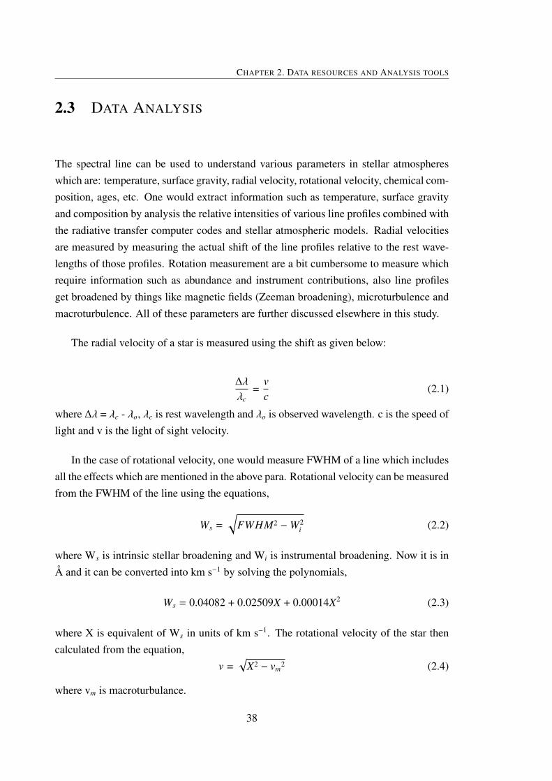
CHAPTER 2. DATA RESOURCES AND ANALYSIS TOOLS
2.3 DATA ANALYSIS
The spectral line can be used to understand various parameters in stellar atmosphereswhich are: temperature, surface gravity, radial velocity, rotational velocity, chemical com-position, ages, etc. One would extract information such as temperature, surface gravityand composition by analysis the relative intensities of various line profiles combined withthe radiative transfer computer codes and stellar atmospheric models. Radial velocitiesare measured by measuring the actual shift of the line profiles relative to the rest wave-lengths of those profiles. Rotation measurement are a bit cumbersome to measure whichrequire information such as abundance and instrument contributions, also line profilesget broadened by things like magnetic fields (Zeeman broadening), microturbulence andmacroturbulence. All of these parameters are further discussed elsewhere in this study.
The radial velocity of a star is measured using the shift as given below:
∆λ
λc=
vc
(2.1)
where ∆λ = λc - λo, λc is rest wavelength and λo is observed wavelength. c is the speed oflight and v is the light of sight velocity.
In the case of rotational velocity, one would measure FWHM of a line which includesall the effects which are mentioned in the above para. Rotational velocity can be measuredfrom the FWHM of the line using the equations,
Ws =
√FWHM2 −W2
i (2.2)
where Ws is intrinsic stellar broadening and Wi is instrumental broadening. Now it is inÅ and it can be converted into km s−1 by solving the polynomials,
Ws = 0.04082 + 0.02509X + 0.00014X2 (2.3)
where X is equivalent of Ws in units of km s−1. The rotational velocity of the star thencalculated from the equation,
v =√
X2 − vm2 (2.4)
where vm is macroturbulance.
38

2.3 DATA ANALYSIS
EQUIVALENT WIDTH
For the current study extraction of the composition is the principal aim. This informationis coded in the spectral line strength which in the abundance studies is known as equiva-lent width with units in Å. The equivalent width is defined as the width of a rectangularspectral line whose area is equal to the integrated area of a spectral line below the con-tinuum flux level (See Figure 2.1). In the Figure, λ0 represents the central wavelength ofthe spectral line. The width of the rectangle represents the Full width at half maximum(FWHM) of a spectral line. The definition is as follows:
Wλ =
∫line
Fλc − Fλ
Fλc
(2.5)
where Wλ is the equivalent width for a given λ and Fλc is the continuum flux.
Figure 2.1: Equivalent width of a spectral line
The spectral line information (λo, FWHM, and Wλ) in the observed spectra are mea-sured using the two most suited options depending on the situation of the spectral profile:SPLOT task in IRAF and/or GAUSSFIT subroutine in IDL. The isolated and clean linesare measured by fitting the single gaussian profile. In some cases, multiple guassian pro-files are computed to deblend the contaminated profiles in the required observed profile.In case of few lines we measured area under the curve of a line profile directly. The finalequivalent widths considered for the analysis are from the mean of two measurements.
The equivalent widths are used to obtain atmospheric parameters and chemical com-position of star. Star’s Te f f , microturbulance, abundance can be obtained from this equa-tion.
39

CHAPTER 2. DATA RESOURCES AND ANALYSIS TOOLS
log(Wλ
λ
)+ log(
vc
) = log(g fλ) −(5040Texc
)χl − 1.826 + log(N) − log(κλU(T )v) (2.6)
where v2 = 2KT/m + ξ2, ξ is microturbulence. The λ is central wavelength of a givenspectral line and Wλ is the equivalent width of a given λ which are measurable quantitiesfrom the spectra. g f is oscillator strength and χl is lower excitation potential which areatomic data of given spectral line. U(T) is a partition function and κλ is opacity which aredistribution function parameters. Texc is excitation temperature and N is the number ofatoms which are atmospheric parameters.
The Saha ionization is used to measure the ionization temperature and surface gravity,
log(
N1
N0
)Pe = 2.5log(Tion) −
5040Tion
+ log(U1
U0
)− 0.1762 (2.7)
Where N0 and N1 are the abundance of particular element in ground state and first excitedstate,respectively. U0 and U1 are the partition function of corresponding states. Tion andI are the ionization temperature and ionization potential, respectively. Pe is the electronpressure which is proportional to gravity (g1/3).
At present, the radiative transfer codes are available where these basic equations areincorporated by assuming the stellar atmospheres in LTE conditions. Determination ofatmospheric parameters and chemical composition using radiative transfer codes requiredatomic data and model atmospheres. A brief description of each tool is given below.
2.3.1 ATOMIC DATA
The spectral lines are principally characterized by three quantities: their wavelengthsassociated spectroscopic classifications; the energies of their upper and lower atomic lev-els; and their oscillator strengths or atomic transition probabilities. The spectral lines thatare formed in the dense gas or plasma depend on additional quantities : line shape andline shift parameters. Of the three principal quantities, atomic transition probabilities aremuch less known than either wavelengths or energy levels. Even for a small percentageof lines for which they are reliably known, the accuracy of the available transition prob-ability data is usually not very high and a number of discrepancies between various dataare encountered.
The spectral lines of Iron, neutral and singly ionized, are abundant in the entire opticalregion of the spectra for which atomic data with accurate log gf values are available in
40

2.3 DATA ANALYSIS
the literature: Fuhr & Wiese (2006), NIST database, VALD database, etc. In this case,we have freedom to choose isolated and clean absorption lines which are suitable formeasurements. For the other elements, due to scarcity, we chose the lines with goodatomic data.
2.3.2 MODEL ATMOSPHERES
The atmosphere of a star is defined as the layer that is sufficiently close to the surfacethat some photons can escape. It is a transition from dense stellar interior to interstellarmedium. The primary layers in the stellar atmosphere are, photosphere, chromosphere,corona, and stellar wind. The atmosphere is the region that produces the stellar spectrum.The physical depths in the atmosphere where the spectral features form depend on theatmospheric conditions: temperature, density, level populations, optical depth etc. Thetheory of stellar atmospheres involves constructing models of the photosphere that takeinto account the effective temperature, Te f f , gravity, g, and elemental abundances. Theassumptions and limitations in the model atmospheres are:
• The thickness of the photosphere is much lesser than the radius of the star, andhence plane parallel geometry. The gravity also constant through out the photo-sphere. The optical depth (τ ∼ infinity) is deep in the atmosphere and τ ∼ 0 at thephotospheric surface. The plane-parallel approximation breaks down for luminous,low surface gravity stars, with extended envelope atmospheres.
• The atmosphere is homogeneous and hence ignores the structures like granulation,starspots etc.
• The outward pressure gradients exactly balances the gravity and hence hydrostaticequilibrium.
• It is in a steady state so the properties do not change with time. The equation ofradiative transfer is independent of time. The atoms and molecules are in statisticalequilibrium. Models assume no rotation, pulsation, expanding envelopes, winds,shocks, and variable magnetic fields etc.
• All energy transport by radiative processes and hence radiative equilibrium. Trans-port by convectionis neglected. Also, neglects the hydrodynamic effects. But thereis much evidence for the existence of velocity fields in the solar atmosphere andmass motions, including convection, are significant in stellar atmospheres, particu-larly in luminous giants.
41
CHAPTER 2. DATA RESOURCES AND ANALYSIS TOOLS
• Under LTE, all the microscopic processes are in detailed balance and the densitiesof energy states are calculated from the Maxwell, Boltzmann, and Saha relations.
An extensive grid of stellar photospheric models was calculated using the ATLAS9stellar atmosphere code which was originally written and developed by Robert. L. Kurucz(Kurucz 1970, 1993). The grid covers a range of effective temperatures from 8000 Kto 35000 K at steps of 250 K and a range of surface gravities (log(g)) from 2.25 dexto 6.25 dex at steps of 0.25 dex. ATLAS9 makes a standard set of assumptions, thatare described above, in modeling. The models were calculated using the standard solarmetallicity ODFs (Opacity Distribution Functions). The abundances of each model areexplicitly set to the solar values for each element. Overall, the differences between themodels calculated at [M/H] = 0 versus other metallicities are not very significant to makeany difference in the abundance analysis. This version of the ATLAS9 code employs theCastelli et al. (1997b,a) convection correction. All models were calculated with a constantmicroturbulent velocity. A velocity of 5 km s−1 was used in models hotter than 9000 Kand a velocity of 2 km s−1 was used in cooler models. A lower value was employed in thecooler models because higher values exceed the thermal velocity of hydrogen in the upperlayers of the model, causing instabilities. The microturbulence value used to calculate themodels does not significantly perturb the abundances calculated from equivalent widths.
2.3.3 MOOG
The study of chemical composition include both Fine analysis and Spectrum Synthesismethods depending on the quality of available data. Equivalent widths were converted toabundances in Fine analysis and line profiles were synthesized to fit the observed profilesin spectrum synthesis method. In this analysis, we used the updated version of LTEraidative transfer code, MOOG which was originally written and developed by Sneden(1973) for his PhD thesis. The version of the MOOG code used is optimized to work withcooler G and K stars. The detailed description of these codes and methods can be foundin Chris. Sneden thesis and in a review article by Castelli & Hack (1990). We brieflydescribe here each of these methods.
FINE ANALYSIS
The method consists of comparing the measured equivalant width of a given line withthe equivalent widths calculated for a given atmospheric model and atomic data. Thesubroutine, abfind, in MOOG solves the radiative transfer problem for spectral lines under
42

2.3 DATA ANALYSIS
the LTE assumptions and calculates the equivalent widths for a given stellar atmosphericmodel. MOOG requires the atmospheric model and linelist as an input. The linelistconsists of wavelength, ion information, excitation potential, oscillator strength/log g f
value and measured equivalent width. For a given stellar model, abundance is modifieduntil the computed equivalant width matches with that of observed equivalent width. Thiscan be achieved by many iterations with some prefixed step value (e.g. 0.1 dex). Weak andmoderate lines would be best for the determination of abundances because their equivalentwidths are not affected by microturbulance and damping constants.
SPECTRUM SYNTHESIS ANALYSIS
This method consists of comparing the observed spectrum with that of the computedspectrum. In this method, fluxes are computed for closeby λ values with similar reso-lution as the observed spectrum which allows the direct comparison. In this synthesis,broadening mechanisms like microturbulance, instrumental broadening, limb darkening,rotational broadening and macroturbulance should be taken into account. Instrumentalbroadening can be represented by a guassian profile, which has the same FWHM as theinstrumental profile that convolved with the observed spectrum. Macroturbulance, thelarge scale structures in the stellar atmospheres, is a random distribution but it can besimulated by gaussian. The rotational broadening can be taken into account by comput-ing the Doppler shifts of the intensities coming from the different parts of the stellar discand then integrating the Doppler shifted intensities to obtain the flux. The emergent in-tensity decreases from the center of the disc to the limb, known as limb darkening, canbe calculated from the available empirical relations. The spectrum synthesis calculationsrequire extensive linelist for a given region. The synthesis of a particular element requiresthe data of different ionized states, with accurate laboratory wavelengths, excitation po-tentials for lower and upper levels, and reliable transition probabilities (gf-values), andbroadening parameters. A large database for both atomic and molecular lines is availablefrom the pioneering work of Kurucz & Bell (1995).
Spectrum synthesis analysis has some advantages over fine analysis in chemical com-position studies. The comparison of computed spectrum with the observed spectrummakes it possible to derive line micro and macro-turbulance, projected rotational veloc-ity, Doppler shifts and abundances from single and blended lines. The continuum level inthe observed spectra can be better estimated, particularly, in case of stars with rapid rota-tion and cool stars whose spectra with numerous metallic lines. The computed spectrumis used to confirm abundances of blended lines obtained with the fine analysis because the
43

CHAPTER 2. DATA RESOURCES AND ANALYSIS TOOLS
comparison of profiles gives much more information than the comparison of equivalentwidths.
We have used the “synth” subroutine in the line synthesis code, MOOG, for computingthe synthesis spectra in our abundance analysis. The inputs to the MOOG are as follows:stellar atmospheric model, abundances of relevant elements, beginning and end points ofthe required region, step size (in wavelength) in the spectrum, width of the spectrum to beconsidered at each point and atomic data similar to fine analysis but without equivalentwidths. For the given inputs, MOOG calculates continuum flux, point by point, separatedby a given step size. The abundances are estimated from MOOG to run for several timesby adjusting the input abundances of elements until the computed spectrum matches thatof observed one.
ATMOSPHERIC PARAMETERS
The atmospheric parameters, Te f f , log g, and microturbulance, are obtained using fineanalysis method by modifying the model atmospheres to satisfy the three constrains:(1) Minimize the slope of A(Fe I) versus Wλ/λ which determine the microturbulance (ξt)because the adopted ξt has a significant effect on the abundances derived from the equiv-alent width of the lines. The strong lines which suffer from saturation has more effectcompared to weaker lines. Therefore, we set the microturbulance of model atmospherewhere the lines with the range of equivalent widths include moderate and strong show notrend.(2) Minimize the slope of A(Fe I) versus LEP which is sensitive to the effective tem-perature because the predicted population in various excitation levels is a function of theexcitation temperature of the stellar atmosphere(3) The median values of A(X I) and A(X II) are equal for the requirement to maintainionization equilibrium (e.g. A(Fe I) = A(Fe II)) which is sensitive to gravity .
METALLICITY
In astronomy, the elements that are heavier than helium are called metals. The measureof the proportion of metals that a star contains is called Metallicity. Iron is the mostabundant heavy element among all the metals and is easily measured in the optical regionof the spectra and hence metallicity is often referred as the relative amount of iron andhydrogen present in the star compared with solar values. Metallicity is denoted as [Fe/H]and is calculated from the following logarithmic formula.
44
2.4 OTHER RESOURCES
[Fe/H] = log(Fe/H)? − log(Fe/H) (2.8)
where [Fe/H] = 0. For example, if the metallicity [Fe/H] = -1 then the abundance ofheavy elements in the star is one tenth that found in the Sun; if [Fe/H] = +1, the heavyelement abundance is 10 times the solar value.
2.4 OTHER RESOURCES
There are few other resources which are extensively used in this thesis that are given inbrief as follows:
HIPPARCOS CATALOG
HIPPARCOS is an acronym for High Precision Parallax Collecting Satellite. Hipparcossatellite mission was launched successfully in August 1989. It observed the celestialsphere for 3.5 years before the mission ended in March 1993. This was the first spacemission dedicated to astrometry. Calculations from observations by the main instrumentgenerated the Hipparcos Catalogue of 118,218 stars charted with the highest precision.An auxiliary star mapper pinpointed many more stars with lesser but still unprecedentedaccuracy, which are given in the Tycho Catalogue which consists 1,058,332 stars. TheTycho 2 Catalogue, completed in 2000, brings the total to 2,539,913 stars, and includes99% of all stars down to magnitude 11.
Accurate measurements of the positions of stars, parallaxes and proper motions areobtained for more than 100 thousand stars from Hipparcos and released the entire data asa catalog in 1997. The data with new reduction techniques which improved the accuracyin errors in the parallaxes. The revised parallaxes were released in 2008.
EVOLUTIONARY TRACKS
The evolutionary tracks are available with Padova and yale-yonseii (YY) groups. Padovatracks computed by Girardi et al. (2000) and Bertelli et al. (2008) are used. Y2 trackscomputed by yale group (Yi et al. 2003) are also used. Padova tracks have the data of thebump whereas no such data is in Y2 tracks. We utilized all these three evolutionary tracksin this study.
45

CHAPTER 2. DATA RESOURCES AND ANALYSIS TOOLS
PUBLIC RESOURCES
This research was made use of material available in the public resources that are follow-ing: (i) the SIMBAD Database , VizieR Service, and Catalogs (access to astronomicalcatalogs), operated at CDS, Strasbourg, France. (ii) The SAO/NASA Astrophysics DataSystem (ADS), which is a Digital Library for Astronomy and Physics, operated by theSmithsonian Astrophysical Observatory (SAO) under a NASA grant. (iii) Two micronall sky survey (2MASS), which is a joint project of the University of Massachusetts andthe Infrared Processing and Analysis Center/California Institute of Technology, fundedby the National Aeronautics and Space Administration and the National Science Founda-tion. (iv) Hipparcos Catalog, data collected from the Hipparcos space mission, funded byEuropean Space Agency (ESA). (V) The Infrared Astronomical Satellite (IRAS), whichis a joint project of the US, UK and the Netherlands. (Vi) IRAF is the Image Reductionand Analysis Facility, a general purpose software system for the reduction and analysisof astronomical data. IRAF is written and supported by the IRAF programming groupat the National Optical Astronomy Observatories (NOAO) in Tucson, Arizona. NOAOis operated by the Association of Universities for Research in Astronomy (AURA), Inc.under cooperative agreement with the National Science Foundation.
46

CHAPTER 3
SURVEY FOR LI-RICH GIANTS
3.1 INTRODUCTION
Li-rich giants are a rare group of stars. There are just about two dozen low mass K- andG- giants that are known to have an anomalously large amount of Li. Many of thesewere discovered accidentally (Hanni 1984). It was the study by Wallerstein & Sneden(1982) which pointed out the unexpected excess of Li in a typical RGB star HD 112127.Li excess in this giant is about 100 times more than the value one would expect fromthe standard theory of stellar evolution and mixing on RGB. The excess, they thoughtcould be due to internal synthesis via Cameron & Fowler (1971) mechanism, and somesort of mixing. They have also pointed out that the suggestion of linking of excess Li tothe planet engulfment (Alexander 1967) is an unlikely scenario. since then, solutions toorigin of Li in giants remained largely very speculative. The main reason for that beingthe lack of sufficient observational data to understand various possibilities.
To address the issue, Brown et al. (1989) initiated a first systematic survey to findout a more number of Li-rich giants among 644 K- and G- giants. Their high resolutionspectroscopic survey resulted in about 10 Li-rich giants which demonstrated the rarity ofLi-rich giants in the solar neighborhood. Other important survey was the Pico Dias survey(PDS) by Gregorio-Hetem et al. (1993) which resulted in half a dozen Li-rich K giants(Reddy & Lambert 2005). Originally, their survey was meant to study Li profile in T Tauristars. Though the post survey resulted in a good number of Li-rich giants, it lacked theuniformity and selection criteria that could be used to draw statistical conclusions suchas a number fraction of Li-rich giants, Li correlation with other properties etc. Also, theabove surveys were pre-Hipparcos leading to uncertain luminosities. As a result samplestars were contaminated by a large number of intermediate mass giants, AGB stars etc.
47

CHAPTER 3. SURVEY FOR LI-RICH GIANTS
Also, the PDS survey was based on a sample of stars that have far-IR (IRAS) colorssimilar to pre-main sequence T Tauri stars. Obviously, the selection bias in the samplemight have led the authors to suggest that Li excess and the IR excess are correlated.Also, some Li-rich K giants were found to have much larger rotational velocities (> 8-10km s−1) than the expected values for typical K giants (about 2 km s−1). It has to be seenhow the three observational properties: high Li, IR excess, and high rotation are related toeach other. Or is it pure coincidental that all the three anomalous properties exist in someof the Li-rich K giants (Brown et al. 1989; Balachandran et al. 2000) Establishing suchcorrelations will constrain theoretical modeling and help to understand the underlyingphysics for the excess Li and also other properties.
This requires a systematic and a well defined survey for Li-rich K giants. Hipparcosspace mission was launched to measure accurate astrometry for about one lakh stars,and its full data was made available in 1997 (Perryman et al. 1997). Unfortunately, nosystematic survey was taken up by any group in the post-Hipparcos period. Given thenumber of speculative ideas for the origin of excess Li in K giants, it became important toventure into such an uniform study to find clues about their origin. Understanding of Liin K giants also has other broader implications such as understanding the stellar structureand evolution of RGB stars, evolution of Li in our Galaxy, and the actual productionof Li at the time of big bang. This study may not address all of these implications butconcentrate on finding clues for its origin.
For the above mentioned reasons, we thought that the study of a controlled but unbi-ased survey sample of K giants would not only increase the number of K giants but alsoconstrain different theoretical ideas for the Li excess in K giants. Therefore, we have setthe following goals for the survey:
a) Adding significant number of Li-rich giants to the existing sample
b) Gathering enough evidence to support or against the hypothesis that the planet en-gulfment could enhance surface Li in K giants
c) Establishing the location of Li enhancement in K giants along the RGB in the HRdiagram
d) Establish the fractional content of Li-rich K giants in the Galaxy
e) Understanding the relation among Li excess and other anomalies such as high rota-tion and infrared excess
f) Study of Li excess and its trend with other abundances like C, N, O and 13C
48
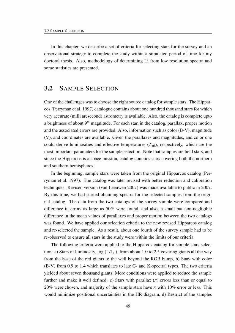
3.2 SAMPLE SELECTION
In this chapter, we describe a set of criteria for selecting stars for the survey and anobservational strategy to complete the study within a stipulated period of time for mydoctoral thesis. Also, methodology of determining Li from low resolution spectra andsome statistics are presented.
3.2 SAMPLE SELECTION
One of the challenges was to choose the right source catalog for sample stars. The Hippar-cos (Perryman et al. 1997) catalogue contains about one hundred thousand stars for whichvery accurate (milli arcsecond) astrometry is available. Also, the catalog is complete uptoa brightness of about 9th magnitude. For each star, in the catalog, parallax, proper motionand the associated errors are provided. Also, information such as color (B-V), magnitude(V), and coordinates are available. Given the parallaxes and magnitudes, and color onecould derive luminosities and effective temperatures (Teff), respectively, which are themost important parameters for the sample selection. Note that samples are field stars, andsince the Hipparcos is a space mission, catalog contains stars covering both the northernand southern hemispheres.
In the beginning, sample stars were taken from the original Hipparcos catalog (Per-ryman et al. 1997). The catalog was later revised with better reduction and calibrationtechniques. Revised version (van Leeuwen 2007) was made available to public in 2007.By this time, we had started obtaining spectra for the selected samples from the origi-nal catalog. The data from the two catalogs of the survey sample were compared anddifference in errors as large as 50% were found, and also, a small but non-negligibledifference in the mean values of parallaxes and proper motion between the two catalogswas found. We have applied our selection criteria to the new revised Hipparcos catalogand re-selected the sample. As a result, about one fourth of the survey sample had to bere-observed to ensure all stars in the study were within the limits of our criteria.
The following criteria were applied to the Hipparcos catalog for sample stars selec-tion: a) Stars of luminosity, log (L/L), from about 1.0 to 2.5 covering giants all the wayfrom the base of the red giants to the well beyond the RGB bump, b) Stars with color(B-V) from 0.9 to 1.4 which translates to late G- and K-spectral types. The two criteriayielded about seven thousand giants. More conditions were applied to reduce the samplefurther and make it well defined: c) Stars with parallax (π) errors less than or equal to20% were chosen, and majority of the sample stars have π with 10% error or less. Thiswould minimize positional uncertainties in the HR diagram, d) Restrict of the samples
49

CHAPTER 3. SURVEY FOR LI-RICH GIANTS
to distances upto 200pc to minimize uncertainties in color due to unaccounted interstel-lar extinction, e) Samples were restricted to magnitudes V∼8.5 or brighter to avoid largeerrors in parallax and also to make it easy for the observations, f) Stars with declinationfrom −60 to +80 deg were chosen to fit observing program with the facilities locatedat +32 degree north (2-m HCT) and +12 degree north (1-m CZT and 2.34-m VBT) lat-itudes, and finally, g) We have culled all the stars with mass greater than 3M and lessthan 0.8M. We have done this by plotting computed stellar evolutionary tracks in the HRdiagram and superposing the selected sample stars. The above criteria resulted in 2000giants. A representative list of the main list is provided in Table 3.1.
3.2.1 SAMPLES ON H-R DIAGRAM
As noted earlier, positions in HR diagram represent the evolutionary stages of stars. Byplotting stars and evolutionary tracks in the form of Luminosity versus Teff , one wouldget a fair idea of stellar mass, age, and also relative evolutionary stages. Therefore, it isimportant to derive luminsoity and Teff for the entire sample stars. Since we have, for allthe stars, parallaxes, apparent magnitude (mv), and color (B-V), it is straight forward toderive log(L/L) and Teff using well known calibrations and a set of equations.
The basic equations used to derive luminosity are given below:
log(L/L) = 0.4(Mbol − Mbol) (3.1)
where Mbol and Mbol are the bolometric magnitudes of the sun and star, respectively.For Mbol, we have adopted a value of 4.74 (see Allen’s astrophysical quantitites (Cox2000)).
Mbol = Vo + BC + 5logπ + 5 (3.2)
where Vo is the visual magnitude of a star corrected for interstellar extinction, BC is thebolometric correction and π is the parallax in arcsec. BC is derived from calibrationsgiven Alonso et al. (1999) below:
BC(v) =−9.93×10⁻²
x+ 2.887×10⁻² + 2.275x − 4.425x2 + 0.3505x[Fe/H]
−5.558×10⁻²[Fe/H] − 5.375×10⁻³[Fe/H]2 (3.3)
where x = log(Teff) - 3.52, [Fe/H] is the metallicity of a star.Teff is derived from (B-V) color taken from Hipparcos catalog, and the calibrations
50

3.2 SAMPLE SELECTION
Tabl
e3.
1:B
asic
data
ofa
few
star
sin
the
sam
ple
surv
ey.
HIP
No
HD
No
π(a
rcse
c)σπ(%
)D
ist
B−
VR
AD
EC
VSp
type
Tef
flo
g(L
/L
)20
8122
610.
0385
1.85
25.9
1.11
0026
16.8
7−
4218
18.4
2.40
K0I
II..
4644
.81.
849
4302
674
794
0.01
087.
2592
.51.
0108
4602
.45−
0202
55.6
5.70
K0I
II:
4619
.41.
647
2841
740
460
0.00
6913
.18
144.
91.
1006
0006
.05
+27
1620
.56.
61K
1III
4758
.91.
754
1214
616
295
0.00
8115
.06
122.
81.
0302
3633
.97−
1439
24.0
6.91
K0I
II47
36.0
1.79
540
407
6928
00.
0051
11.1
119
6.0
1.27
008
1456
.71−
3541
19.6
6.80
K1/
K2I
II43
27.5
1.95
753
240
9436
30.
0126
3.40
79.3
0.91
310
5325
.04−
0215
18.0
6.12
K0I
II49
77.7
1.35
343
388
7579
00.
0067
9.53
149.
20.
980
0850
18.9
4−
4443
16.1
7.50
K0I
II48
40.8
1.36
945
439
7991
70.
0145
3.72
68.8
1.08
409
1536
.76−
3834
11.7
4.92
K1I
II46
43.0
1.76
969
3990
330.
0081
12.1
412
2.3
1.19
901
2923
.49
+25
1631
.26.
66K
2III
4442
.61.
785
1154
4422
0363
0.00
848.
2911
9.0
1.31
523
2304
.56
+12
1850
.25.
09K
3III
4257
.72.
139
1144
4921
8792
0.00
6412
.55
155.
51.
330
2310
42.6
2+
1735
40.0
5.68
K4I
II42
34.9
2.28
237
901
6290
20.
0122
6.72
82.1
1.37
807
4602
.16−
0646
20.2
5.49
K5I
II41
63.7
1.73
159
2863
190.
0093
5.39
106
1.08
0116
12.6
2+
8708
44.0
6.20
K2I
II:
4588
.91.
590
7511
913
6514
0.01
366.
4273
.31.
1815
2102
.01
0042
56.1
5.35
K3I
II44
56.0
1.64
722
240
3079
00.
0067
9.07
149.
21.
0104
4706
.85−
5908
13.6
6.80
K0I
II47
17.1
1.75
978
3710
212
0.00
7711
.42
129.
80.
970
0140
49.7
4+
4501
08.7
8.13
K0I
II48
60.7
1.09
515
677
2092
40.
0079
9.04
125.
71.
152
0321
58.7
9−
1527
31.4
7.26
K0I
II45
22.3
1.24
712
070
1620
20.
0061
9.91
163.
91.
122
0235
38.4
4−
1456
41.9
6.84
K0/
K1I
II45
74.7
1.41
284
455
1563
620.
0087
8.66
115.
31.
187
1715
58.9
2+
2708
03.6
6.57
K2I
II44
62.7
1.62
346
363
8184
10.
0051
14.6
194.
51.
154
0927
14.1
9−
3347
28.5
7.16
K2I
II45
18.9
1.82
611
2731
2161
740.
0082
6.60
121.
81.
167
2249
46.2
3+
5554
09.7
5.43
K1I
II44
96.5
2.03
496
014
1842
930.
0071
6.56
141.
61.
274
1931
19.3
6+
5018
23.7
5.55
K1I
II43
21.2
2.23
252
338
9235
40.
0063
510
.79
157.
41.
315
1041
48.3
1+
6826
36.8
5.74
K3I
II42
57.7
2.37
9
51
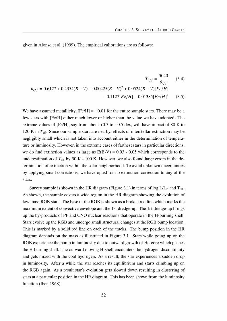
CHAPTER 3. SURVEY FOR LI-RICH GIANTS
given in Alonso et al. (1999). The empirical calibrations are as follows:
Te f f =5040θe f f
(3.4)
θe f f = 0.6177 + 0.4354(B − V) − 0.00425(B − V)2 + 0.0524(B − V)[Fe/H]
−0.1127[Fe/H] − 0.01385[Fe/H]2 (3.5)
We have assumed metallicity, [Fe/H] = −0.01 for the entire sample stars. There may be afew stars with [Fe/H] either much lower or higher than the value we have adopted. Theextreme values of [Fe/H], say from about +0.3 to −0.5 dex, will have impact of 80 K to120 K in Teff . Since our sample stars are nearby, effects of interstellar extinction may benegligibly small which is not taken into account either in the determination of tempera-ture or luminosity. However, in the extreme cases of farthest stars in particular directions,we do find extinction values as large as E(B-V) = 0.03 - 0.05 which corresponds to theunderestimation of Teff by 50 K - 100 K. However, we also found large errors in the de-termination of extinction within the solar neighborhood. To avoid unknown uncertaintiesby applying small corrections, we have opted for no extinction correction to any of thestars.
Survey sample is shown in the HR diagram (Figure 3.1) in terms of log L/L and Teff .As shown, the sample covers a wide region in the HR diagram showing the evolution oflow mass RGB stars. The base of the RGB is shown as a broken red line which marks themaximum extent of convective envelope and the 1st dredge-up. The 1st dredge-up bringsup the by-products of PP and CNO nuclear reactions that operate in the H-burning shell.Stars evolve up the RGB and undergo small structural changes at the RGB bump location.This is marked by a solid red line on each of the tracks. The bump position in the HRdiagram depends on the mass as illustrated in Figure 3.1. Stars while going up on theRGB experience the bump in luminosity due to outward growth of He-core which pushesthe H-burning shell. The outward moving H-shell encounters the hydrogen discontinuityand gets mixed with the cool hydrogen. As a result, the star experiences a sudden dropin luminosity. After a while the star reaches its equilibrium and starts climbing up onthe RGB again. As a result star’s evolution gets slowed down resulting in clustering ofstars at a particular position in the HR diagram. This has been shown from the luminosityfunction (Iben 1968).
52
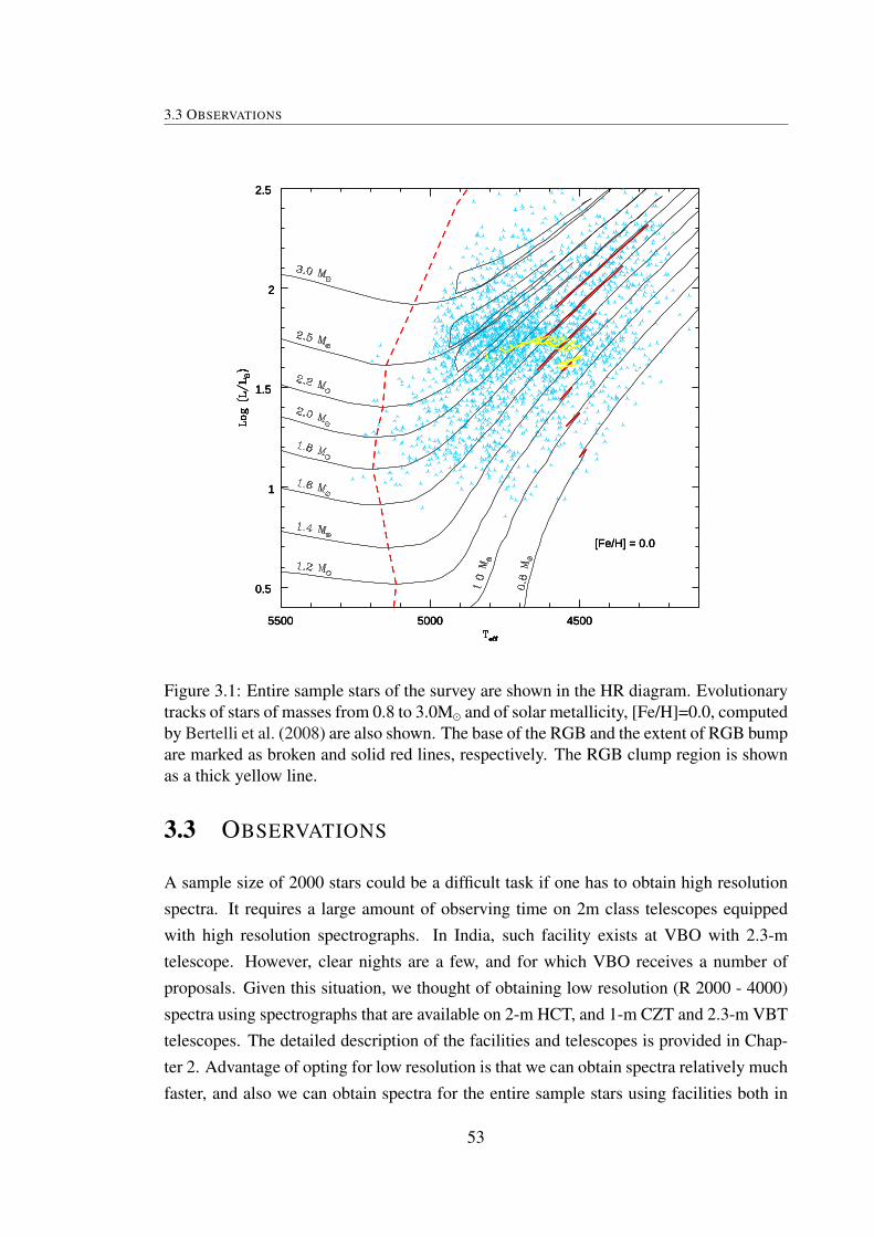
3.3 OBSERVATIONS
5500 5000 4500
0.5
1
1.5
2
2.5
[Fe/H] = 0.0
5500 5000 4500
0.5
1
1.5
2
2.5
[Fe/H] = 0.0
5500 5000 4500
0.5
1
1.5
2
2.5
[Fe/H] = 0.0
Figure 3.1: Entire sample stars of the survey are shown in the HR diagram. Evolutionarytracks of stars of masses from 0.8 to 3.0M and of solar metallicity, [Fe/H]=0.0, computedby Bertelli et al. (2008) are also shown. The base of the RGB and the extent of RGB bumpare marked as broken and solid red lines, respectively. The RGB clump region is shownas a thick yellow line.
3.3 OBSERVATIONS
A sample size of 2000 stars could be a difficult task if one has to obtain high resolutionspectra. It requires a large amount of observing time on 2m class telescopes equippedwith high resolution spectrographs. In India, such facility exists at VBO with 2.3-mtelescope. However, clear nights are a few, and for which VBO receives a number ofproposals. Given this situation, we thought of obtaining low resolution (R 2000 - 4000)spectra using spectrographs that are available on 2-m HCT, and 1-m CZT and 2.3-m VBTtelescopes. The detailed description of the facilities and telescopes is provided in Chap-ter 2. Advantage of opting for low resolution is that we can obtain spectra relatively muchfaster, and also we can obtain spectra for the entire sample stars using facilities both in
53

CHAPTER 3. SURVEY FOR LI-RICH GIANTS
northern and southern part of the country. But the disadvantage is that we will not be ableto get accurate Li abundances, and also, in the low resolution, we can’t have Li informa-tion in stars where Li profile is weak. We may not get the full Li distribution among theRGB stars which limits us to say something on anamolously low lithium among a groupof RGB stars. Also, determination of abundances of other elements will not be possible.However, our interest in this study is primarly extracting RGB stars with excess Li andsearch for clues for its origin. Thus, our planned study of medium to strong Li-profilestars, and later subject, the potential high Li stars, to high resolution spectroscopy forconfirmation and detailed studies is well justified.
Table 3.2: Journal of ObservationsHD RA DEC V Exp time SNR Yr of obs
HCT + HFOSC + 67s + Gr9 + Gr11 + 1K×3K CCD186648 19 46 21.82 −19 45 39.2 4.87 90 250 2007183491 19 28 57.08 +24 46 07.3 5.82 180 250 2007198236 20 44 33.08 +69 45 06.8 6.50 260 250 2007196912 20 39 59.83 +08 26 49.4 6.85 300 250 2007194056 20 21 14.12 +52 24 38.0 7.61 420 250 2007193342 20 17 00.58 +56 54 17.0 8.07 480 250 2007224533 23 58 40.41 −03 33 20.9 4.88 100 300 2006187614 19 49 55.81 +27 05 06.6 6.46 240 200 200716302 02 37 34.35 +20 34 29.8 6.92 270 200 2007146388 16 15 28.68 +18 48 29.9 5.72 150 200 200922572 03 37 50.37 +00 08 28.0 7.18 360 250 200619551 03 09 00.94 +12 51 34.7 7.23 510 150 2006947 00 14 22.39 +76 01 19.8 7.72 510 100 2006
1-m CZT + UAGS + 120µ + 1800lmm−1 + 1K×1K CCD23319 03 42 50.12 −37 18 48.0 4.59 900 200 200970002 08 18 17.39 −35 27 06.1 5.59 1200 200 200988399 10 10 37.70 −41 42 53.8 5.98 1500 200 200945984 06 27 04.14 −58 00 07.6 5.82 1800 200 200922663 03 37 05.68 −40 16 28.2 4.57 900 200 200620640 03 17 26.6 −47 45 06.3 5.84 900 150 2008
VBT + OMRS + 300µ + 1200lmm−1 + 1K×1K CCD159194 17 35 06.28 −38 47 58.3 6.76 300 300 200926833 04 11 58.89 −53 24 43.5 7.07 600 300 200977120 08 58 30.75 −50 48 25.2 7.57 720 300 2009133904 15 09 23.25 −57 04 01.6 8.00 900 300 200928700 04 29 20.04 −46 30 55.3 6.13 420 350 2007
Spectra of entire sample were taken over a period of about 3 years, during 2006-2009.Our initial goal was to complete observations in over two years. However, we couldn’t
54

3.3 OBSERVATIONS
accomplish partly due to sky conditions at VBO, where monsoons take away significantportion of observing time, and partly due to the revised astrometry data. The journal ofobservations for a sample of stars is given in Table 3.2 which contains star’s identity,coordinates (RA and Dec), visual magnitude, exposure time, signal to noise ratio, andyear of observations. Below, we provide a brief description of observations that werecarried out with three different instruments mounted on three different telescopes.
6600 6650 67000
0.5
1
1.5
6600 6650 67000
0.5
1
1.5
6600 6650 67000
0.5
1
1.5
6600 6650 67000
0.5
1
1.5
Figure 3.2: A sample spectra taken from HFOSC on 2-m HCT. Li line at 6707 Å, Ca linesat 6717 Å and 6572 Å, and Fe line 6592 Å are marked. Note the strength variation of Liline relative to other lines. All other lines including Hα vary in strength very little or nochange at all.
3.3.1 SPECTRA FROM HFOSC ON 2-M HCT
Stars in the survey sample with declination between −20 to +80 deg were observed withthe 2-m HCT telescope. HCT is equipped with Himalayan Faint Object SpectrographCamera or HFOSC, a dedicated instrument for imaging and spectroscopy. It has a 2K× 4K CCD with a pixel size of 15 µ (For details see Chap 2). Spectra were obtained inEchelle mode with a combination of Grism (Gr9) and cross disperser (Gr11) combined
55
CHAPTER 3. SURVEY FOR LI-RICH GIANTS
with slit width of 0.77′′. This resulted in spectra with a resolution of R ≈ 3500 coveringspectral range from 4500 Å to 9000 Å over 8 orders. Since stars are brighter we could getvery good Signal-to-Noise Ratio (SNR) with exposure times as small as 5-10 minutes.All the spectra are of SNR of 200 to 300 as measured at 6700 Å.
3.3.2 SPECTRA FROM UAGS ON 1-M CZT
This aim was to obtain spectra for the entire sample stars within 2 years using the facilitiesthat were available as the 1-m telescope. Most of the bright stars, both northern andsouthern stars, were observed using medium resolution Zeiss Universal Astro GratingSpectrograph (UAGS) which is available at the Cassegrain focus. Spectra were recordedon 1K × 1K CCD with a pixel size of 24 µm. We have used a grating with 1800l mm−1
which gives a dispersion of 0.6 Å per pixel which has a resolution of about R=5000. Wehave obtained spectra centered at 6700 Å which covers Ca and Hα lines apart from Liline at 6707 Å. The typical SNR for most of the spectra is about 100 or more at 6700 Å .Exposure times for a given star of same mv is relatively much larger for UAGS comparedto other two spectrographs due to its high dispersion and smaller aperture of the telescope.
3.3.3 SPECTRA FROM OMRS ON 2.3-M VBT
Other telescope that was used in this study was 2.3-m Vainu Bappu telescope (VBT) atVBO. The VBT is equipped with low resolution OMR spectrograph at the Cassegrainfocus, and a Tetronix CCD of 1K × 1K with a pixel size of 24µm. We have used a gratingwith 1200 lmm−1 which gives the dispersion of 1.4 Å per pixel (R 2000) about one thirdof UAGS. With this resolution only strong Li profile could be detected. A few hundredspectra were obtained with the VBT and it is quite efficient with minimal overheads.
3.3.4 REDUCTIONS
Spectra were obtained with three different instruments with different resolutions and cov-erage, and with different modes such as echelle (orders) and long slit modes. The re-duction procedure differs slightly from one set of observations to the other set. All theraw two dimensional spectra were reduced with the use of an image reduction softwareknown as IRAF for Image Reduction and Analysis Facility developed by NOAO, USA.During observations, spectra of Fe-Ne arc lamp were obtained for wavelength calibra-tion purpose. Fe-Ne spectrum contains a number of emission lines that have accurately
56

3.3 OBSERVATIONS
6550 6600 6650 6700
0
1
2
3
4
6550 6600 6650 6700
0
1
2
3
4
6550 6600 6650 6700
0
1
2
3
4
6550 6600 6650 6700
0
1
2
3
4
Figure 3.3: A few spectra taken from UAGS on 1-m telescope at VBO. Due to slightlyhigher resolution, relatively well separated lines are seen.
measured wavelengths. Also, obtained were images of dark and flat field to correct forthermal noise and pixel-to-pixel variation in the CCD, respectively.
IRAF is a full fledged software that contains number of packages with which one canaccomplish all the tasks necessary to convert raw images to the one dimensional rela-tive flux versus wavelength. As a first step, all the images were corrected for dark, andapplied normalized flat images to correct for pixel-to-pixel variation. The dark and flatcorrected images were reduced to one dimensional spectra, including Fe-Ne arc, usingaperture extraction tools available within IRAF. Emission lines in Fe-Ne arc spectrumwere identified and assigned wavelengths. A polynomial fit was obtained between pixelpositions versus wavelength of emission features. The derived polynomial was used toconvert program stars spectra into flux versus wavelengths. Two or three such polynomi-als were obtained for each night to see if there are any changes over the night. In general,we have found the instruments are quite stable and therefore no changes are noticed inthe derived polynomials. Similar procedure was applied to all the data. Finally, to obtainrelative strengths of different lines, spectra were normalized to unity i.e continuum fitting
57
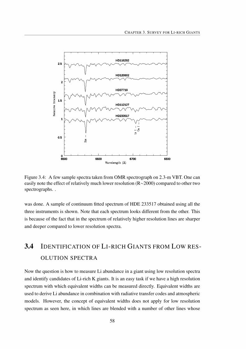
CHAPTER 3. SURVEY FOR LI-RICH GIANTS
6500 6600 6700 68000
0.5
1
1.5
2
2.5
HD233517
HD112127
HD37719
HD120602
HD116292
6500 6600 6700 68000
0.5
1
1.5
2
2.5
HD233517
HD112127
HD37719
HD120602
HD116292
6500 6600 6700 68000
0.5
1
1.5
2
2.5
HD233517
HD112127
HD37719
HD120602
HD116292
6500 6600 6700 68000
0.5
1
1.5
2
2.5
HD233517
HD112127
HD37719
HD120602
HD116292
Figure 3.4: A few sample spectra taken from OMR spectrograph on 2.3-m VBT. One caneasily note the effect of relatively much lower resolution (R∼2000) compared to other twospectrographs. .
was done. A sample of continuum fitted spectrum of HDE 233517 obtained using all thethree instruments is shown. Note that each spectrum looks different from the other. Thisis because of the fact that in the spectrum of relatively higher resolution lines are sharperand deeper compared to lower resolution spectra.
3.4 IDENTIFICATION OF LI-RICH GIANTS FROM LOW RES-
OLUTION SPECTRA
Now the question is how to measure Li abundance in a giant using low resolution spectraand identify candidates of Li-rich K giants. It is an easy task if we have a high resolutionspectrum with which equivalent widths can be measured directly. Equivalent widths areused to derive Li abundance in combination with radiative transfer codes and atmosphericmodels. However, the concept of equivalent widths does not apply for low resolutionspectrum as seen here, in which lines are blended with a number of other lines whose
58
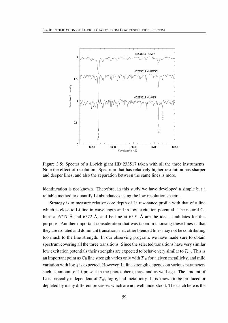
3.4 IDENTIFICATION OF LI-RICH GIANTS FROM LOW RESOLUTION SPECTRA
6550 6600 6650 6700 67500
0.5
1
1.5
2
HD233517 - UAGS
HD233517 - HFOSC
HD233517 - OMR
6550 6600 6650 6700 67500
0.5
1
1.5
2
HD233517 - UAGS
HD233517 - HFOSC
HD233517 - OMR
Figure 3.5: Spectra of a Li-rich giant HD 233517 taken with all the three instruments.Note the effect of resolution. Spectrum that has relatively higher resolution has sharperand deeper lines, and also the separation between the same lines is more.
identification is not known. Therefore, in this study we have developed a simple but areliable method to quantify Li abundances using the low resolution spectra.
Strategy is to measure relative core depth of Li resonance profile with that of a linewhich is close to Li line in wavelength and in low excitation potential. The neutral Calines at 6717 Å and 6572 Å, and Fe line at 6591 Å are the ideal candidates for thispurpose. Another important consideration that was taken in choosing these lines is thatthey are isolated and dominant transitions i.e., other blended lines may not be contributingtoo much to the line strength. In our observing program, we have made sure to obtainspectrum covering all the three transitions. Since the selected transitions have very similarlow excitation potentials their strengths are expected to behave very similar to Teff . This isan important point as Ca line strength varies only with Teff for a given metallicity, and mildvariation with log g is expected. However, Li line strength depends on various parameterssuch as amount of Li present in the photosphere, mass and as well age. The amount ofLi is basically independent of Teff , log g, and metallicity. Li is known to be produced ordepleted by many different processes which are not well understood. The catch here is the
59

CHAPTER 3. SURVEY FOR LI-RICH GIANTS
Tabl
e3.
3:D
eriv
edlin
ede
pth
ratio
san
dL
iabu
ndan
ces
forK
gian
tsth
atar
eus
edin
deriv
ing
rela
tions
.
HD
RA
DE
CV
A(L
i)E
xptim
eL
i/671
7L
i/657
2L
i/659
2H
FOSC
UA
GS
HFO
SCU
AG
SO
MR
HFO
SCH
FOSC
787
0012
09.9
86−
1756
17.8
05.
291.
8090
1200
0.95
749
0.93
92–
0.96
117
1.01
321
4082
706
0508
.229
+59
2335
.56
6.32
1.60
180
900
1.00
717
1.01
521
2335
1708
2246
.710
0+
5304
49.1
99.
704.
2248
027
000.
8040
790.
6740
00.
9192
160.
8119
40.
8565
110
8471
1227
42.0
00+
0836
37.0
06.
362.
0018
018
001.
0228
61.
0736
41.
0043
471.
0283
11.
0861
310
9703
1236
17.0
811
+51
3053
.41
8.60
2.82
420
2700
0.94
5698
0.93
822
0.97
8636
0.94
619
1.00
1121
2712
5355
.615
9+
2646
48.0
66.
892.
7024
024
000.
8942
080.
7965
20.
9765
240.
8931
70.
9579
611
6292
1323
01.2
222−
1744
05.3
55.
362.
8290
600
1.05
964
1.12
853
1.01
4482
1.05
681.
1229
712
0602
1350
24.6
228
+05
2949
.69
6.01
1.90
9060
01.
0176
11.
0696
11.
0109
271.
0076
31.
0632
512
6868
1428
12.5
243−
0213
40.3
34.
842.
4060
300
1.01
932
1.04
382
0.99
9792
1.00
206
1.04
657
1468
5016
1900
.468
1-1
452
21.8
816.
018
2.00
120
600
0.95
617
0.93
5602
...0.
9553
31.
0389
9
60

3.4 IDENTIFICATION OF LI-RICH GIANTS FROM LOW RESOLUTION SPECTRA
assumption of constant metallicity. This is reasonable for a given sample which is locatedin the solar neighborhood. Our estimates based on Stromgren photometry suggest thatvast majority of stars in the sample have metallicity close to solar value of [M/H]=0.0.Unfortunately, we do not have Stromgren photometry for the entire sample stars. Also,looking at the sample spectra one may notice that metallic lines such as Fe and Ca arealmost constant but Li varies from one spectrum to the other (Figure 3.2). Thus, the ratioof core depths of Li at 6707 Å and other Ca I lines will provide reliable information on Liabundance for a given star.
To understand how core depth ratios of Li line at 6707 Å with Ca I lines and Fe I linerelate with Li abundances, we have observed a sample of K giants, for which Li abun-dances are available based on high resolution spectra, with low resolution spectrographsmounted on the three facilities that were mentioned before. Empirical relations betweencore depth ratios and the abundances taken from the literature have been derived. Thesample K giants that are used in the empirical relations include most of the known Li-richK giants for which accurate Li abundances are available. Empirical relations derived forHCT spectra for ratios of line core depths of Li and other candidate lines core depths aregiven below. The linear regression fits, obtained using S IXLIN, show that core depthratios are directly proportional to the amount of Li present in the atmosphere. Scatterin the fits seems to be very similar for all the three relations but the relation between Li(6707 Å)/Ca (6717 Å) and Li abundances is relatively a better fit. This might be due tothe strength of Ca line at 6717 Å and hence is well seen in the low resolution spectrum.
A(Li) =
((1.201 ± 0.02) − (Li/Ca6572)
0.096 ± 0.009
)(3.6)
A(Li) =
((1.248 ± 0.015) − (Li/Ca6592)
0.094 ± 0.072
)(3.7)
A(Li) =
((1.164 ± 0.009) − (Li/Ca6717)
0.083 ± 0.005
)(3.8)
The above relations are valid for stars of constant metallicity which is closer to solarvalue. Also, the above relations are valid only for stars of abundances greater than 0.6dex. This is because, in the HCT spectra, we could detect Li lines only if the Li abundancein the star is more than 0.6 dex. The empirical relations are shown in Fig 3.6 and bottompanel of Fig 3.7. A similar procedure was followed for the data collected from 1-mand 2.3-m telescopes. The derived relations are shown in top two panels of Fig 3.7.Relations derived from 2.3-m spectra have relatively more scatter due to significantly
61

CHAPTER 3. SURVEY FOR LI-RICH GIANTS
lower resolution compared to other spectrographs. As a result, in many cases, even thestrong Ca or moderate Li lines could not be properly resolved. This puts the minimumdetection limit of 1.5 dex for Li abundance. This still works for us as we have defined Kgiant with Li abundance log ε (Li) ≥ 1.5 as the Li-rich K giant and does not voilate ourgoal of identifying Li-rich K giants among RGB stars.
0 1 2 3 4 50.7
0.8
0.9
1
1.1
1.2
A(Li)
0 1 2 3 4 50.7
0.8
0.9
1
1.1
1.2
A(Li)
0 1 2 3 4 50.7
0.8
0.9
1
1.1
1.2
A(Li)
0 1 2 3 4 50.7
0.8
0.9
1
1.1
1.2
A(Li)
0 1 2 3 4 50.7
0.8
0.9
1
1.1
1.2
A(Li)
0 1 2 3 4 50.7
0.8
0.9
1
1.1
1.2
A(Li)
0 1 2 3 4 50.7
0.8
0.9
1
1.1
1.2
A(Li)
0 1 2 3 4 50.7
0.8
0.9
1
1.1
1.2
A(Li)
Figure 3.6: Empirical relations derived for line depth ratios and Li abundances of knownLi-rich giants for spectra obtained from HCT . In the top panel, relation of core depth ratioof Li to Ca line ( 6572 ) and Li abundances is shown. The bottom panel shows relationfor Li to Fe line (6592 Å). The fit coefficients are provided on top of the panels.
A(Li) =
((1.323 ± 0.05) − (Li/Ca6717)
0.16 ± 0.019
)(3.9)
A(Li) =
(1.068 ± 0.01 − (Li/Ca6717)
0.0345 ± 0.002
)(3.10)
As noted earlier, we have observed the entire sample over a period of three yearsmaking use all the facilities at our disposal. Out of 2000 sample stars, spectra for 1100stars were obtained from 2-m HCT, 500 spectra from 1-m at VBO, and the rest of the 400stars spectra came from 2.3-m VBT telescope. Line depth ratios for the entire spectra
62
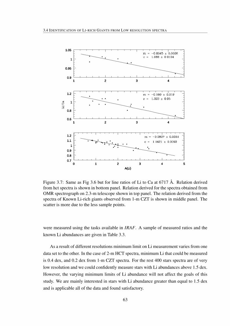
3.4 IDENTIFICATION OF LI-RICH GIANTS FROM LOW RESOLUTION SPECTRA
A(Li)
0 1 2 3 4 50.7
0.8
0.9
1
1.1
1.2
1 2 3 40.6
0.8
1
1.2
1 2 3 40.9
0.95
1
1.05
A(Li)
0 1 2 3 4 50.7
0.8
0.9
1
1.1
1.2
1 2 3 40.6
0.8
1
1.2
1 2 3 40.9
0.95
1
1.05
A(Li)
0 1 2 3 4 50.7
0.8
0.9
1
1.1
1.2
1 2 3 40.6
0.8
1
1.2
1 2 3 40.9
0.95
1
1.05
Figure 3.7: Same as Fig 3.6 but for line ratios of Li to Ca at 6717 Å. Relation derivedfrom hct spectra is shown in bottom panel. Relation derived for the spectra obtained fromOMR spectrograph on 2.3-m telescope shown in top panel. The relation derived from thespectra of Known Li-rich giants observed from 1-m CZT is shown in middle panel. Thescatter is more due to the less sample points.
were measured using the tasks available in IRAF. A sample of measured ratios and theknown Li abundances are given in Table 3.3.
As a result of different resolutions minimum limit on Li measurement varies from onedata set to the other. In the case of 2-m HCT spectra, minimum Li that could be measuredis 0.4 dex, and 0.2 dex from 1-m CZT spectra. For the rest 400 stars spectra are of verylow resolution and we could confidently measure stars with Li abundances above 1.5 dex.However, the varying minimum limits of Li abundance will not affect the goals of thisstudy. We are mainly interested in stars with Li abundance greater than equal to 1.5 dexand is applicable all of the data and found satisfactory.
63

CHAPTER 3. SURVEY FOR LI-RICH GIANTS
Table 3.4: Measurements of line ratios and derived Li abundance of sample starsSpectrograph HD Teff Lum Li/Ca A(Li)
HFOSC
101151 4243 2.47 1.12151 0.44101112 4649 1.73 1.1085 0.61101341 4733 1.68 1.10286 0.68101321 4828 1.31 1.08893 0.86115319 4857 1.47 1.07366 1.07117304 4703 1.79 1.06299 1.21118536 4484 1.92 1.04725 1.41100470 4693 1.80 No detection102096 4972 1.19 No detection10348 4778 2.07 No detection
UAGS
38313 4615 1.54 1.1905 0.9079524 4360 2.08 1.1637 1.0723697 4735 1.31 1.1450 1.1913004 4539 1.46 1.1314 1.27115912 4604 1.99 1.1136 1.3885563 4500 1.86 1.0736 1.64
OMR 51367 4655 1.78 0.9688 3.08
3.5 RESULTS AND DISCUSSION
Once the relations are established between ratio of line depths and the known Li abun-dances, it is now straight forward to derive Li abundance of program stars for a given linedepth ratio. Relations were verified using K giants which are not used in obtaining therelations but have known Li abundances derived from independent methods. Agreementbetween literature abundances and the abundances derived from the relations obtained inthis study are satisfactory within about ±0.3 dex in Li abundance.
Table 3.5: Statistical analysis of Sample starsTelescope Samples Li detection Li-free Li-rich
HCT 1100 250 750 11VBT 500 10 450 2CZT 400 100 300 2
Respective relations are used to derive Li abundances from spectra obtained fromdifferent telescopes. Sample results are shown in Table 3.4 for each data set. In the caseof HCT data set, only 25% of K giants showed detectable Li i.e., log ε(Li) ≥ 0.5. Out of1100 K giants only 20 giants showed Li above 1.2 dex and we assign them as potentialcandidates that belong to Li-rich K giants group, and 11 have Li abundance more than 2.0
64

3.5 RESULTS AND DISCUSSION
0.5 1.0 1.5 2.0 2.5 3.0 3.5A(Li)
0
20
40
60
80
No.
of G
iant
s
Figure 3.8: Li abundance of HCT samples are represented as Histogram. The distributionof the sample showing Gaussian with peak Li abundance at 0.6 dex. Note the Li-richgiants have occupied the tail portion.
dex which are assigned as Li-rich K giants. A distribution function of Li for HCT dataset is shown in Figure 3.8. As shown in the distribution, just about 2% of giants found tohave Li more than the expected value of about 1.5 dex. Rest of the K giants, with Li lessthan 1.5 dex, are treated as normal giants. A few more Li-rich K giants (2 from 1-m dataset, 2 from 2.3-m data set) were added to the list. A consolidated Li distribution is shownin Figure 3.9. Giants with Li abundance less than the minimum detectability are excludedfrom the distribution i.e., giants with Li abundance more than 0.5 dex (HCT data set),0.3 dex (1-m data set), and 1.5 dex (2.3-m data set) are only included in the distribution.The distribution for a full set of data is shown in Figure 3.9. This is very similar to thedistribution for a sub-set of data given in Figure 3.8. Based on the kind of data that wehave with us, we draw the following statistics: a) In about 70% of K giants, we found Linull detection. b) about 20% K giants show Li abundance between 0.6 - 0.8 dex, c) about10% giants have Li between 0.8 - 1.4 dex, and d) about 1 - 2% of total giants have logε(Li) ≥1.5. A total of 15 giants were assigned as Li-rich K giant candidates.
From the Li distributions shown in Figures and the statistics given above, one canmake two important conclusions: 1) Very few giants are there beyond the maximumexpected Li limit of 1.5 dex suggesting rarity of Li-rich K giants, and 2) Distributionpeaks at about Li abundance 0.6-0.7 dex which is in good agreement with the standardtheoretical model predictions. However, we can’t make a suggestion or confirm, based onthe data set presented here, results of anomalously low Li abundances in K giants (Brown
65

CHAPTER 3. SURVEY FOR LI-RICH GIANTS
0.5 1.0 1.5 2.0 2.5 3.0 3.5A(Li)
0
20
40
60
80
No.
of G
iant
s
Figure 3.9: Li abundance of all samples are represented as Histogram. The distribution ofthe sample showing Gaussian with peak Li abundance at 0.7 ± 0.2 dex. Note the Li-richgiants have occupied the tail portion.
et al. 1989).
Table 3.6: Derived parameters of new Li-rich giantsHD Teff Lum Li/Ca A(Li) Telescopehd40168 4771.50 2.15802 1.0599 1.24 HCThd88476 4941.12 1.89466 1.02526 1.74 HCThd133086 4831.96 1.72413 1.02285 1.77 HCThd118319 4752.32 1.71014 1.00512 2.07 UAGShd12203 4804.46 1.71598 1.0102 1.89 HCThd107484 4504.67 1.80961 0.99814 2.04 HCThd145457 4731.41 1.63329 0.974466 2.35 HCThd37719 4655.10 1.77948 0.968824 3.08 OMRhd51367 4530.49 1.61089 0.985891 2.61 OMRhd167304 4729.52 1.95527 0.936517 2.81 HCThd150902 4664.27 1.85361 0.93185 2.85 HCThd170527 4812.28 1.71506 0.902105 3.30 HCThd10437 4660.60 1.79629 0.883247 3.54 HCThd8676 4705.07 1.70139 0.846645 3.70 HCThd77361 4549.62 1.69125 0.818115 3.30 UAGS
To further understand the sample, we have separated all the new Li-rich K giants fromthe sample and presented in Table 3.6 along with parameters such as Teff , Luminosity, linedepth ratio, and derived Li abundance. Entire sample giants along with the newly identi-fied Li-rich K giants are shown in the HR diagram. Li-rich K giants are shown as solidblue circles indicating the amount of Li with circle size. Results shown in Figure 3.10
66
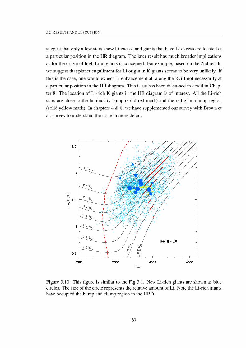
3.5 RESULTS AND DISCUSSION
suggest that only a few stars show Li excess and giants that have Li excess are located ata particular position in the HR diagram. The later result has much broader implicationsas for the origin of high Li in giants is concerned. For example, based on the 2nd result,we suggest that planet engulfment for Li origin in K giants seems to be very unlikely. Ifthis is the case, one would expect Li enhancement all along the RGB not necessarily ata particular position in the HR diagram. This issue has been discussed in detail in Chap-ter 8. The location of Li-rich K giants in the HR diagram is of interest. All the Li-richstars are close to the luminosity bump (solid red mark) and the red giant clump region(solid yellow mark). In chapters 4 & 8, we have supplemented our survey with Brown etal. survey to understand the issue in more detail.
5500 5000 4500 4000
0.5
1
1.5
2
2.5
[Fe/H] = 0.0
5500 5000 4500 4000
0.5
1
1.5
2
2.5
[Fe/H] = 0.0
5500 5000 4500 4000
0.5
1
1.5
2
2.5
[Fe/H] = 0.0
5500 5000 4500 4000
0.5
1
1.5
2
2.5
[Fe/H] = 0.0
Figure 3.10: This figure is similar to the Fig 3.1. New Li-rich giants are shown as bluecircles. The size of the circle represents the relative amount of Li. Note the Li-rich giantshave occupied the bump and clump region in the HRD.
67

CHAPTER 3. SURVEY FOR LI-RICH GIANTS
3.6 CONCLUSIONS
We have completed a largest survey for Li-rich K giants among RGB stars. A sampleof 2000 giants were chosen from the revised Hipparcos catalogue. Color and luminositycriteria were applied to the catalogue in such a way that sample stars are of late G- and K-type, and of wide luminosity range, from the base of RGB to well beyond the luminositybump. A novel strategy was followed to complete the entire survey program. Strategywas to obtain low resolution spectra and use relative line depth of Li line profile at 6707Å to near by Ca or Fe lines. With this strategy we could get spectra for the entire samplein relatively shorter time.
The survey resulted in 15 new Li-rich K giants increasing the current Li-rich giants bya factor of two. Also, we confirm earlier survey by Brown et al., and establish from thisstudy that the Li-rich stars are rare, just about 2%, in the Galaxy. Another important resultis that Li-rich stars occupy a particular position in the HR diagram. The new Li-rich starsare located close to the luminosity bump and the hotter ones overlap with the red clumpstars. Results suggest that planet engulfment or some external trigger is a very unlikelyscenario for Li-excess in the RGB stars. We conclude from the results that Li excessis most probably triggered by events in the stellar interior at this particular evolutionarystage. In other chapters we discuss possible scenario such as Li production during bumpevolution, Li production at the time of He-flash at the tip of the RGB, etc.
68
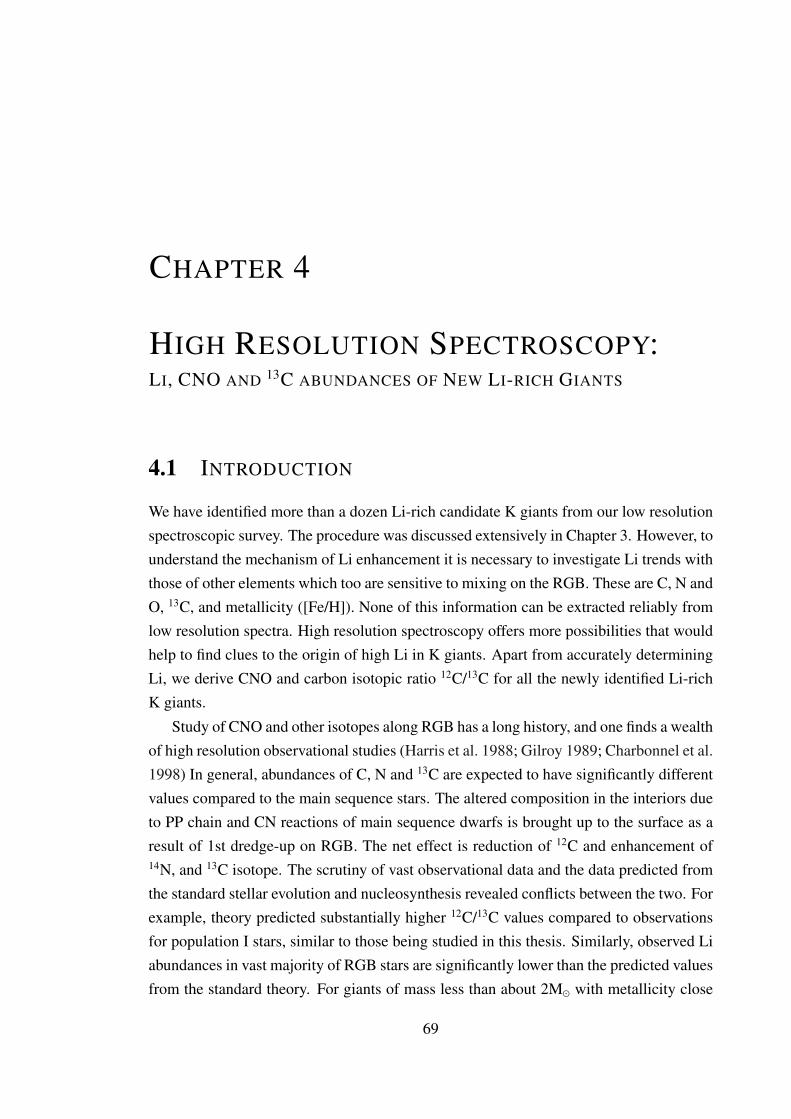
CHAPTER 4
HIGH RESOLUTION SPECTROSCOPY:LI, CNO AND 13C ABUNDANCES OF NEW LI-RICH GIANTS
4.1 INTRODUCTION
We have identified more than a dozen Li-rich candidate K giants from our low resolutionspectroscopic survey. The procedure was discussed extensively in Chapter 3. However, tounderstand the mechanism of Li enhancement it is necessary to investigate Li trends withthose of other elements which too are sensitive to mixing on the RGB. These are C, N andO, 13C, and metallicity ([Fe/H]). None of this information can be extracted reliably fromlow resolution spectra. High resolution spectroscopy offers more possibilities that wouldhelp to find clues to the origin of high Li in K giants. Apart from accurately determiningLi, we derive CNO and carbon isotopic ratio 12C/13C for all the newly identified Li-richK giants.
Study of CNO and other isotopes along RGB has a long history, and one finds a wealthof high resolution observational studies (Harris et al. 1988; Gilroy 1989; Charbonnel et al.1998) In general, abundances of C, N and 13C are expected to have significantly differentvalues compared to the main sequence stars. The altered composition in the interiors dueto PP chain and CN reactions of main sequence dwarfs is brought up to the surface as aresult of 1st dredge-up on RGB. The net effect is reduction of 12C and enhancement of14N, and 13C isotope. The scrutiny of vast observational data and the data predicted fromthe standard stellar evolution and nucleosynthesis revealed conflicts between the two. Forexample, theory predicted substantially higher 12C/13C values compared to observationsfor population I stars, similar to those being studied in this thesis. Similarly, observed Liabundances in vast majority of RGB stars are significantly lower than the predicted valuesfrom the standard theory. For giants of mass less than about 2M with metallicity close
69

CHAPTER 4. HIGH RESOLUTION SPECTROSCOPY:LI, CNO AND 13C ABUNDANCES OF NEW LI-RICH GIANTS
to solar value, standard theory predicts 12C/13C in the range of 20-30. This is a reductionof 12C/13C ratio by a factor of about 3 from its main-sequence value of 12C/13C ≈ 89.However, the number of studies on open clusters and field giants show much smallervalues. For example, Wallerstein & Morell (1994) 23 giants in an open cluster showedalmost a constant value of 12C/13C ≈ 12. In some cases even much smaller values (e.g;Kumar & Reddy 2009. Reason for low values of 12C/13C and Li compared to standardtheory is attributed to extra mixing of various kinds (see e.g; Boothroyd & Sackmann1999; Palacios et al. 2006; Eggleton et al. 2008). By invoking special mixing mechanism,these models could reproduce low values observed in majority of RGB stars.
However, there are a very small group of giants which show extremely large amountof Li which is totally unexpected in K giants with such deep mixing process. Also, thereare a few giants of Pop I, which have extremely low values of 12C/13C ≈ 4-8. None ofthe models constructed so far could reach that low values. Also, it is quite necessary todevelop a model that could simultaneously predict low values of 12C/13C and very highvalues of Li. To constrain models in this direction, it would be an important exercise forus to derive accurate Li, CNO, and 12C/13C, and [Fe/H] for all the new K giants. Theseare the first measurements of its kind for these 15 K giants. In this chapter, we describehigh resolution spectroscopic observations, abundance derivation, Li trends with otherelemental abundances and isotopic ratios, and kinematics.
4.1.1 A BRIEF ACCOUNT OF NEWLY IDENTIFIED LI-RICH K GIANTS
Our survey for finding Li-rich K giants among RGB stars resulted in 15 new candidateLi-rich giants. Basic data of the program stars is given in Table 4.1. Below we provide abrief account of each of the newly identified Li-rich K giants.
HD 8676 : No previous studies on any stellar parameters including Li. No references arefound in literature.HD 10437: Pakhomov et al. (2011) study on space velocities show that this star is asso-ciated with Hercules moving group.HD 12203: No previous studies on any stellar parameters including Li. No references arefound in literature.HD 37719: It has been checked for its binarity and found with null detection (Makarov& Kaplan 2005; Frankowski et al. 2007).HD40168: It is a faint x-ray source with 0.06±0.01 cts/s which is listed in ROSAT Allsky survey bright star catalog (RASS) (Voges et al. 1999). Haakonsen & Rutledge (2009)studied the cross association of RASS sources with 2MASS sources quantitatively and
70
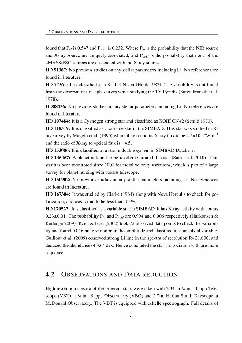
4.2 OBSERVATIONS AND DATA REDUCTION
found that Pid is 0.547 and Pnoid is 0.232. Where Pid is the probability that the NIR sourceand X-ray source are uniquely associated, and Pnoid is the probability that none of the2MASS/PSC sources are associated with the X-ray source.HD 51367: No previous studies on any stellar parameters including Li. No references arefound in literature.HD 77361: It is classified as a K1III CN star (Houk 1982). The variability is not foundfrom the observations of light curves while studying the TY Pyxidis (Surendiranath et al.1978).HD88476: No previous studies on any stellar parameters including Li. No references arefound in literature.HD 107484: It is a Cyanogen strong star and classified as KOIII CN+2 (Schild 1973).HD 118319: It is classified as a variable star in the SIMBAD. This star was studied in X-ray survey by Maggio et al. (1990) where they found its X-ray flux to be 2.5×10⁻¹⁶Wm−2
and the ratio of X-ray to optical flux is −4.5.HD 133086: It is classified as a star in double system in SIMBAD Database.HD 145457: A planet is found to be revolving around this star (Sato et al. 2010). Thisstar has been monitored since 2001 for radial velocity variations, which is part of a largesurvey for planet hunting with subaru telescope.HD 150902: No previous studies on any stellar parameters including Li. No referencesare found in literature.HD 167304: It was studied by Clarke (1964) along with Nova Herculis to check for po-larization, and was found to be less than 0.3%.HD 170527: It is classified as a variable star in SIMBAD. It has X-ray activity with counts0.23±0.01. The probability Pid and Pnoid are 0.994 and 0.006 respectively (Haakonsen &Rutledge 2009). Koen & Eyer (2002) took 72 observed data points to check the variabil-ity and found 0.0169mag variation in the amplitude and classified it as unsolved variable.Guillout et al. (2009) observed strong Li line in the spectra of resolution R≈21,000, anddeduced the abundance of 3.64 dex. Hence concluded the star’s association with pre-mainsequence.
4.2 OBSERVATIONS AND DATA REDUCTION
High resolution spectra of the program stars were taken with 2.34-m Vainu Bappu Tele-scope (VBT) at Vainu Bappu Observatory (VBO) and 2.7-m Harlan Smith Telescope atMcDonald Observatory. The VBT is equipped with echelle spectrograph. Full details of
71

CHAPTER 4. HIGH RESOLUTION SPECTROSCOPY:LI, CNO AND 13C ABUNDANCES OF NEW LI-RICH GIANTS
Tabl
e4.
1:A
bsol
ute
mag
nitu
dean
dL
umin
osity
ofne
wL
i-ri
chgi
ants
from
basi
cda
taav
aila
ble
inH
ippa
rcos
cata
log
HD
No
HIP
No
VSp
type
π(”
)σπ
σπ(%
)M
vσ
Mv
BC
σBC
Mbo
lσ
Mbo
llo
g(L
/L
)σ
L
8676
6647
7.77
K0I
II4.
270.
7414
.60.
9221
0.37
69-0
.310
80.
0392
0.61
140.
3789
1.65
540.
1516
1043
780
526.
57K
1III
6.72
0.59
11.7
0.70
680.
1917
-0.3
226
0.04
090.
3842
0.19
61.
7463
0.07
8412
203
9343
6.75
G5
6.58
0.64
9.7
0.84
110.
2122
-0.3
082
0.03
780.
533
0.21
551.
6868
0.08
6237
719
2649
97.
62K
1III
4.23
0.63
14.9
0.75
170.
324
-0.4
050.
0514
0.34
670.
3281
1.76
130.
1312
4016
828
149
6.88
G5
3.75
0.64
17.0
-0.2
498
0.37
11-0
.335
20.
0422
-0.5
851
0.37
352.
134
0.14
9451
367
3329
86.
99K
1/K
2III
7.09
0.46
11.0
1.24
320.
1423
-0.4
063
0.05
240.
8369
0.15
161.
5652
0.06
0777
361
4429
06.
20K
1III
CN
9.25
0.43
8.0
1.03
070.
1029
-0.4
433
0.05
710.
5874
0.11
771.
665
0.04
7188
476
5001
96.
86G
8III
4.97
0.72
14.5
0.34
180.
3152
-0.2
306
0.02
90.
1112
0.31
651.
8555
0.12
6610
7484
6024
07.
72K
0III
CN
4.06
0.75
18.4
0.76
260.
4016
-0.4
115
0.05
30.
3512
0.40
511.
7595
0.16
211
8319
6640
56.
48K
0III
7.58
0.55
12.7
0.87
830.
1588
-0.4
098
0.05
160.
4685
0.16
71.
7126
0.06
6813
3086
7313
66.
83K
06.
250.
436.
80.
8094
0.15
07-0
.280
90.
0355
0.52
850.
1548
1.68
860.
0619
1454
5779
219
6.57
K0I
II7.
980.
459.
21.
080.
1241
-0.3
150.
0394
0.76
50.
1302
1.59
40.
0521
1509
0281
156
7.93
G5
3.36
0.55
16.3
0.56
170.
356
-0.3
855
0.04
920.
1762
0.35
941.
8295
0.14
3816
7304
8924
66.
36K
0III
6.07
0.34
8.0
0.27
590.
1233
-0.3
105
0.03
97-0
.034
50.
1295
1.91
380.
0518
1705
2790
274
6.84
K0
6.31
0.40
6.3
0.84
010.
1391
-0.3
310.
0417
0.50
910.
1452
1.69
630.
0581
72

4.2 OBSERVATIONS AND DATA REDUCTION
the VBT and the spectrograph (Rao et al. 2005) are given in Chapter 2. All the spectrawere taken with a slit width of 60µ which is about 4 pixels on CCD with a 15µ pixel sizewhich gives spectral resolution R 60,000 (R=λ/∆λ). Full spectrum covers over a widerange from 4000Å to 9000Å but with large gaps between orders. Therefore, we requiretwo set-ups to have full optical spectrum. High quality spectra with S/N 300-500 and res-olution R 60,000 were obtained from 2.7-m Harlan Smith Telescope which is equippedwith Coude echelle spectrograph (Tull et al. 1995). Spectra covers from 3500Å to 9500Åwith small gaps between the orders beyond 5600 Å. Again to cover all the importanttransitions we required two wavelength set-ups. Along with program spectra, we haveobtained twilight solar spectrum for easy identification of wavelengths of line profiles.For the purpose of wavelength calibration, we have obtained Th-Ar arc spectra at regularintervals. Flat field images and bias frames were obtained at the beginning and end ofeach night. For the purpose of identifying and removing of atmospheric lines, couple ofhot stars with very high rotation were observed. The journal of observations is given inTable 4.2.
Table 4.2: Journal of ObservationsHD HIP RA DEC V Observatory Exp time
88476 50019 10:12:42.5 +28:14:31.2 6.87 McDonald/VBT 720/2700170527 90274 18:25:10.1 +64:50:18.3 6.87 McDonald/VBT 1200/2700167304 89246 18:12:42.6 +41:08:48.6 6.356 McDonald/VBT 900/2700150902 81156 16:34:30.2 +77:39:14.2 7.93 McDonald/VBT 1500/3600133086 73136 14:56:48.4 +74:54:03.3 6.843 McDonald/VBT 1200/270040168 28149 05:56:54.7 -08:23:02.4 6.881 McDonald/VBT 900/2700145457 79219 16:10:03.9 +26 44 33.9 6.584 McDonald/VBT 900/270051367 33298 06 55 36.5 -33 48 24.7 6.99 McDonald 180077361 44290 09:01:11.4 -26:39:49.3 6.206 McDonald/VBT 900/27008676 6647 01:25:18.2 -14:59:38.8 7.77 McDonald/VBT 1800/270010437 8052 01:43:21.4 +59:37:58.4 6.57 McDonald/VBT 1200/2700107484 60240 12:21:10.1 +41:28:59.2 7.72 McDonald/VBT 900/2700118319 66405 13:36:50.6 -34:28:03.9 6.48 VBT 270012203 9343 01:59:58.4 +06:02:07.7 6.76 McDonald/VBT 1200/270037719 26499 05:38:08.9 -47:42:51.4 7.62 VBT 2700
Entire two dimensional raw images were reduced to one dimensional flux versuswavelength using spectral image reduction tools available in IRAF. Images were re-moved off dark current using bias frames and pixel-to-pixel variation was taken off usingflat field images. Details on dark and flat images are given in Chapter 2. Once the imageswere corrected for dark current and flat fields, images were inspected for any scattered
73

CHAPTER 4. HIGH RESOLUTION SPECTROSCOPY:LI, CNO AND 13C ABUNDANCES OF NEW LI-RICH GIANTS
light. Scattered light effect is seen in the red part of McDonald spectra which was re-moved by fitting polynomials to the spectral orders using tasks such as “apscatter” inIRAF. Now the spectra is ready for extraction. The extracted spectrum is flux versus pix-els. To convert pixels to wavelength we used Th-Ar comparison spectrum. Wavelengthsfor Th-Ar emission lines are known from the laboratory measurements. A 3rd or 4thorder polynomial wavelength solution for each Th-Ar spectrum was produced for eachnight. Program spectra were wavelength calibrated with the Th-Ar polynomial solutions.Before making the spectra to work with we require to normalize the spectrum to unityor continuum fitted. This is because of the fact that the way the equivalent width (Wλ)has been defined. However, fitting the continuum to the cool stars such as ours is a trickyissue as one must be sure about the shallow dips. For a reference we used a very highquality and high resolution spectrum of Arcturus (Hinkle et al. 2000). A couple of con-tinuum fitted spectra are shown in Figure 4.1. The reduced spectra are further processedto correct for the telluric contamination by dividing the object spectra with the hot starspectra. Entire spectra are brought to laboratory wavelengths by correcting radial motionof stars. The measurement of radial velocities is discussed later in this chapter.
4.3 ATMOSPHERIC AND OTHER STELLAR PARAMETERS
Stellar atmospheric parameters like Teff , log g, and microturbulence velocity (ξt) are nec-essary for the selection of representative atmospheric model and hence quantitative chem-ical composition of stellar photospheres are derived. Also, required are the radial androtational velocities. Radial velocities (Rv) help to accurately identify weak transitionsof trace elements and measure equivalent widths. Also, Rvs are required for computingkinetic motion to determine stellar population in the disk. Rotational velocities are impor-tant in the case of abundance determination by spectrum synthesis method. Atmosphericparameters like Teff and log g can be derived either from photometry or from high reso-lution spectroscopy. Draw back in the photometric values is the uncertainty in extinctionand the errors in the calibrations. However, photometric values are model independentand less cumbersome to derive. On the other hand, values derived from spectroscopy de-pend on model choice and accuracy in the measured equivalent widths. Here we describehow we have obtained the parameters through both photometry as well as spectroscopy.Finally, we adopt spectroscopy values since photometric temperatures are found to bemore effected from extinction.
74
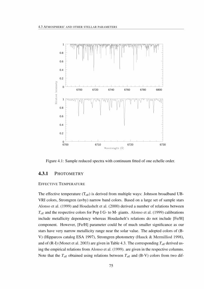
4.3 ATMOSPHERIC AND OTHER STELLAR PARAMETERS
6700 6720 6740 6760 6780 68000
0.2
0.4
0.6
0.8
1
6700 6710 6720 67300
0.2
0.4
0.6
0.8
1
Figure 4.1: Sample reduced spectra with continuum fitted of one echelle order.
4.3.1 PHOTOMETRY
EFFECTIVE TEMPERATURE
The effective temperature (Teff) is derived from multiple ways: Johnson broadband UB-VRI colors, Stromgren (uvby) narrow band colors. Based on a large set of sample starsAlonso et al. (1999) and Houdashelt et al. (2000) derived a number of relations betweenTeff and the respective colors for Pop I G- to M- giants. Alonso et al. (1999) calibrationsinclude metallicity dependency whereas Houdashelt’s relations do not include [Fe/H]component. However, [Fe/H] parameter could be of much smaller significance as ourstars have very narrow metallicity range near the solar value. The adopted colors of (B-V) (Hipparcos catalog ESA 1997), Stromgren photometry (Hauck & Mermilliod 1998),and of (R-I) (Monet et al. 2003) are given in Table 4.3. The corresponding Teff derived us-ing the empirical relations from Alonso et al. (1999). are given in the respective columns.Note that the Teff obtained using relations between Teff and (B-V) colors from two dif-
75

CHAPTER 4. HIGH RESOLUTION SPECTROSCOPY:LI, CNO AND 13C ABUNDANCES OF NEW LI-RICH GIANTS
ferent studies with (Alonso et al. 1999) and without metallicity term (Houdashelt et al.2000) agree very well within ±50 K suggesting very little effect of [Fe/H]. Only for a fewstars (b-y) colors are available and the Teff derived are in good agreement with the (B-V)temperatures. However, Teff obtained from (R-I) colors are found to be systematicallyhigher than both the (B-V) and (b-y) temperatures. The average difference is about ±120K. One reason we can readily think of is that interstellar or circumstellar extinction whichcaused more absorption in Johnson “B” and “V” or stromgren “b” and “y” bands leadingto estimation of cooler temperatures. Color (R-I) seems to be least affected and hencehotter temperatures.
Table 4.3: Derived temperatures from various photometric colors.HD B-V err R-I b-y TB−V
a TB−Vb Tb−y
b TR−Ib
8676 1.051 0.013 0.50 0.641 4744 4704 4710 482510437 1.075 0.007 0.50 0.679 4696 4659 4589 482512203 0.999 0.012 0.47 0.624 4850 4803 4768 494537719 1.078 0.012 0.51 – 4690 4654 – 478540168 1.016 0.010 0.47 0.660 4815 4770 4649 494651367 1.148 0.005 — – 4557 4529 – 467677361 1.137 0.008 0.55 – 4578 4558 – 464288476 0.931 0.005 0.44 0.581 4995 4940 4924 5079107484 1.163 0.005 0.55 – 4530 4503 – 4642118319 1.026 0.006 0.47 0.640 4795 4751 4714 4946133086 0.985 0.010 0.46 – 4880 4850 – 4989145457 1.037 0.005 0.48 – 4772 4730 – 4904150902 1.073 0.015 0.51 0.682 4700 4663 4580 4785167304 1.038 0.007 0.50 – 4770 4728 – 4824170527 0.995 0.011 0.46 – 4858 4811 – 4989
aHoudashelt (2000)bAlonso et al. (1999)
SURFACE GRAVITY
Surface gravity (log g) of program stars has been derived from photometry as well asspectroscopy. In the case of photometry, one requires parallaxes and bolometric mag-nitudes. Bolometric corrections are estimated from calibrations given in Alonso et al.(1999). Basic parameters such as parallaxes, visual magnitude, absolute magnitude ob-tained from the distance modulus, bolometric corrections (BC), bolometric magnitudes,and the derived luminosities of the individual stars and the associated errors are sum-marized in Table 4.1. Errors in luminosity are mainly from the errors in parallaxes and
76

4.3 ATMOSPHERIC AND OTHER STELLAR PARAMETERS
magnitudes. The mean error in luminosity is less than 0.1.
Now it is straight forward to determine surface gravity with standard relations involv-ing Teff , mass, log L/L i.e., L ∝ R2 T4 and g ∝M/R2:
logg = logLL
+ logMM
+ 4logTe f f − 10.61 (4.1)
Where Te f f is the mean of the temperatures given in Table 4.3. Luminosity is re-measuredfor the above corresponding temperature. Stellar masses are estimated using evolutionarytracks computed from Bertelli et al. (2008). The log g values are also derived from em-pirical calibrations (Hekker & Melendez 2007) for giants where the relations are derivedfrom the observations of large number of sample giants which is a function of temperaturealone:
loggIII = −26.332 + 1.117×10⁻²Te f f − 1.064 × 10⁻⁶Te f f2 (4.2)
Table 4.4 summarizes log g values derived from two different methods, mean Te f f , lumi-nosity and mass of a star. We see good agreement between the log g values derived fromthe two relations.
Table 4.4: Derived surface gravities from astrometry and photometry .HD Tmean log(L/L) M/M logga loggb
8676 4746 1.670 1.8 2.694 2.71410437 4692 1.766 1.9 2.602 2.65412203 4842 1.703 2.2 2.749 2.80737719 4710 1.745 2.0 2.652 2.67440168 4795 2.130 3.0 2.474 2.76451367 4587 1.574 1.6 2.680 2.51877361 4592 1.658 1.5 2.570 2.52588476 4985 1.865 3.0 2.807 2.909107484 4558 1.773 1.5 2.442 2.476118319 4802 1.678 2.1 2.774 2.770133086 4906 1.689 2.3 2.840 2.859145457 4802 1.597 1.8 2.788 2.771150902 4682 1.826 2.1 2.582 2.641167304 4774 1.924 2.5 2.594 2.743170527 4886 1.680 2.2 2.823 2.843
aFrom standard relationbHekker 2007
77

CHAPTER 4. HIGH RESOLUTION SPECTROSCOPY:LI, CNO AND 13C ABUNDANCES OF NEW LI-RICH GIANTS
4.3.2 HIGH RESOLUTION SPECTROSCOPY
RADIAL VELOCITY
It is important to measure radial shifts in a given spectrum as the shifts are used to identifyline profiles. Observed positions in terms of wavelengths for about 100 well definedand isolated lines have been recorded by fitting Gaussian. The corresponding laboratorywavelength positions of the identified lines were taken from different sources (Reddyet al. 2003; Allende Prieto et al. 2002; NIST). The differences between observed andlaboratory wavelength positions are the radial shifts in wavelength. Shifts are convertedto radial velocities (see Chapter 2). In Table 4.5 we provide measurements of a few linesof rest wavelength, observed wavelength, measured shift, and derived radial velocities.The mean of Rv is obtained by fitting the Gaussian distribution to the histogram of radialvelocities (See Figure 4.2). The observed radial velocities are corrected for Earth’s motionto get heliocentric radial velocities. In Table 4.6, we have provided star’s radial velocitywith respect to local standard of rest (LSR) by taking into account of Sun’s motion in thespace. For a few stars radial velocities exist already in the literature. The literature valuesare in good agreement with the values from this study within ±1 km s−1. This may alsosuggest that these are not binaries. For some stars the values given in Table 4.6 are thefirst measurements.
-36.0 -35.5 -35.0 -34.5 -34.0 -33.5 -33.0Radial Velocity
0
2
4
6
8
10
12
No.
of d
ata
poin
ts
#, µ, σ= 63, -34.5028, 0.4858
Figure 4.2: Mean radial velocity is determined by fitting the guassian to the distributionof radial velocity from various individual lines.
78

4.3 ATMOSPHERIC AND OTHER STELLAR PARAMETERS
Table 4.5: Measurement of line shifts for few selected lines to derive radial velocity.λrest λobs δλ Rv
4432.566 4432.057 -0.508789 -34.41154481.610 4481.089 -0.520996 -34.85154635.850 4635.314 -0.536133 -34.67084656.980 4656.439 -0.541016 -34.82784798.265 4797.710 -0.555176 -34.6874802.880 4802.325 -0.554688 -34.62325234.620 5234.021 -0.599121 -34.31235358.120 5357.496 -0.624023 -34.91485379.574 5378.957 -0.617188 -34.39465414.070 5413.439 -0.630859 -34.93255473.901 5473.271 -0.629883 -34.49725525.540 5524.914 -0.625977 -33.96285661.348 5660.693 -0.655273 -34.69955741.850 5741.188 -0.662109 -34.56995753.121 5752.462 -0.65918 -34.34955809.220 5808.549 -0.671387 -34.64785849.690 5849.009 -0.681152 -34.90865927.786 5927.111 -0.675293 -34.15235952.716 5952.037 -0.678711 -34.18146027.060 6026.366 -0.693848 -34.51276082.710 6082.006 -0.704102 -34.70246149.250 6148.539 -0.710938 -34.66016159.380 6158.666 -0.713867 -34.74576247.560 6246.844 -0.71582 -34.3496271.283 6270.560 -0.723145 -34.56926369.460 6368.734 -0.726074 -34.17436496.469 6495.737 -0.732422 -33.79916591.330 6590.560 -0.77002 -35.02276699.142 6698.379 -0.763184 -34.15316725.360 6724.592 -0.768066 -34.23766793.260 6792.471 -0.788574 -34.80056837.009 6836.229 -0.779785 -34.19246857.250 6856.469 -0.780762 -34.13426971.936 6971.141 -0.794922 -34.18157112.173 7111.356 -0.816895 -34.43387802.510 7801.585 -0.924805 -35.53347807.920 7807.022 -0.897949 -34.4776
KINEMATIC MOTION AND GALACTIC ORBITAL PARAMETERS
We have computed space motion of each of the program stars to investigate whether Li-rich behavior is anyway related to their membership to either thin disk, thick disk or thehalo populations (see Reddy et al. 2003, 2006). The three velocity components of space
79

CHAPTER 4. HIGH RESOLUTION SPECTROSCOPY:LI, CNO AND 13C ABUNDANCES OF NEW LI-RICH GIANTS
Table 4.6: Derived radial velocities along with literature values
StarVr Vhelio σVr Vrlit σVr
(km s−1) (km s−1) (km s−1) (km s−1) (km s−1)8676 12.25 -7.93 0.4 — —
10437 2.25 -1.60 0.51 -2.6 0.312203 -44.75 -59.78 0.5 — —37719 62.35 53.74 0.45 — —40168 66.00 42.78 0.5 — —51367 44.03 58.71 0.5 — —77361 -1.43 -23.34 0.5 -24.3 0.688476 31.97 4.19 0.39 4.7 0.3
107484 10.10 10.90 0.5 9.8 0.3118319 19.20 22.68 0.5 21.8 0.6133086 -1.76 -9.67 0.50 -9.9 0.3145457 -23.15 -2.87 0.55 -3.6 0.3150902 -34.52 -40.53 0.43 — —167304 -59.80 -49.67 0.42 -48.9 0.3170527 -53.30 -51.72 0.5 -52.1 0.6
velocity U (velocity radially outward from the Galactic center), V (velocity along theGalactic rotation), and W (velocity perpendicular to the Galactic plane) are computedusing the data from Hipparcos catalog: parallaxes and propermotions, and radial veloc-ities given in Table 4.6. The space velocities (U,V,W) with respect to LSR are given inTable 4.7. Solar motion of U, V, W (-10,5.2,7.2) km s−1 derived by Dehnen & Binney(1998) is used. The Galactic orbital parameters are computed by assuming sun’s distanceof 8.5 kpc from the center and the derived kinematics. Probability of a star belongingto either of the three populations in the Galaxy has been computed following the detailsgiven in Reddy et al. (2006). Probability (Pthin, Pthick, orPhalo) of ≥ 0.7 is considered for astar to belong to a particular component population: thin disk, thick disk or halo. Com-puted probabilities are given in Table 4.7. Except HD 12203, all the giants belong to thethin disk component.
ATOMIC DATA AND EQUIVALENT WIDTHS
Atomic data such as central wavelengths, excitation potentials and oscillator strengths(log g f ) are the main input data in the derivation of abundances. In case of moleculeswe require dissociation energies. Other important input is the line strength or equivalentwidths (Wλ) of line profiles in the spectrum. In Table 4.8 we have given atomic dataof selected lines: central wavelength, ion number, lower excitation potential, logg f , andmeasured equivalent widths.
80

4.3 ATMOSPHERIC AND OTHER STELLAR PARAMETERS
Table 4.7: Space velocities, orbital parameters, and probability distribution in GalaxyHD Ulsr Vlsr Wlsr Zmax Rapo Rper Pthick Pthin Phalo
8676 -16.70 -4.00 12.90 0.26 8.82 7.86 0.00989 0.99008 0.0000210437 40.50 -41.00 -14.80 0.12 9.00 5.61 0.03512 0.96476 0.0001012203 -15.40 -49.20 59.30 0.62 8.64 5.48 0.83065 0.16422 0.0051237719 17.20 -42.00 -9.60 0.14 8.59 5.76 0.02493 0.975001 0.0000640168 24.60 -17.50 -3.60 0.08 8.92 7.16 0.01043 0.98954 0.0000251367 22.30 -44.00 -1.30 0.03 8.65 5.63 0.02473 0.97520 0.00007
107484 18.40 -44.30 19.00 0.29 8.64 5.62 0.04045 0.95942 0.00011118319 -23.00 -21.90 -0.60 0.06 8.65 6.63 0.01126 0.98870 0.00002133086 -16.00 5.50 -5.80 0.11 9.02 8.30 0.00768 0.99230 0.00001145457 13.00 9.40 15.20 0.15 9.16 8.23 0.01004 0.98993 0.00002150902 -31.50 -38.20 6.60 0.17 8.77 5.94 0.02213 0.97780 0.00006167304 -27.10 -48.90 -14.30 0.13 8.56 5.31 0.04283 0.95703 0.00013170527 29.90 -53.60 1.10 0.07 8.71 5.03 0.04197 0.95789 0.00013
77361 -44.60 17.40 -5.00 0.05 10.67 7.78 0.01035 0.98961 0.0000288476 10.40 -9.50 -4.10 0.16 8.68 7.69 0.00834 0.99163 0.00001
ATMOSPHERIC PARAMETERS
Atmospheric parameters like Teff, log g, microturbulent velocity (ξt) and metallicity ([M/H])have been derived using spectral line analysis. Determination of atmospheric parametersfrom high resolution spectrum requires a set of well defined lines with a wide range ofWλs and low excitation potentials (LEP). The neutral (Fe I) and singly ionized (Fe II) ironlines satisfy the above criteria as Fe I lines are numerous in any given spectrum. The nextbest element that is represented by large number of clean lines is nickle (Ni I).
We have adopted Fe I and Fe II lines from Reddy et al. (2003) and Allende Prieto et al.(2002). They have compiled a list of FeI and FeII that are unblended (verified using solarand Arcturus spectrum) and have accurate log g f values either measured in laboratory orderived from inverting solar spectrum. For computation of theoretical Wλ we have usedcomputer code called MOOG (version 2002) originally developed by Sneden (1973).Stellar models were taken from Kuruz data base (Kurucz 1994) which are computed fromATLAS9 code developed by Robert Kurucz. Models are based on LTE.
Effective Temperature: Abundances for a set Fe I lines were obtained for stellar modelsof given log g, ξt and [Fe/H] values but for a set of Teffs. Initial Teff and log g are thevalues derived from photometry. The best value of Teff for a given star is the one forwhich abundances are independent of LEPs (see Figure 4.3). To have minimal effect ofξt on the derivation of Teff , it is important to choose only weak lines for this purpose. Inthe derivation of Teff , we have used about 40 lines with LEP starting from 1.0 eV to 5.0
81

CHAPTER 4. HIGH RESOLUTION SPECTROSCOPY:LI, CNO AND 13C ABUNDANCES OF NEW LI-RICH GIANTS
Table 4.8: Atomic data of selected lines and their equivalent widths for few sample Li-richgiants
λIon
LEPlog gf Ref
Wλ(mÅ)(Å) (ev) 8676 10437 12203 88476 133086
5778.458 26.000 2.590 -3.450 R03 70.400 75.60 58.35 51.57 66.345358.120 26.000 3.300 -3.160 R03 34.700 40.60 26.18 23.94 35.485466.990 26.000 3.573 -2.230 C02 73.800 79.80 59.40 56.83 74.125849.690 26.000 3.695 -2.930 R03 27.870 35.23 18.30 18.15 28.006857.250 26.000 4.076 -2.040 R03 52.320 58.70 40.28 38.37 52.086793.260 26.000 4.076 -2.330 C02 33.100 40.70 24.10 23.71 35.956725.360 26.000 4.103 -2.170 R03 42.390 47.39 32.42 31.72 44.265858.790 26.000 4.220 -2.180 R03 35.300 39.88 26.60 22.42 36.095705.460 26.000 4.301 -1.360 C02 68.300 71.30 57.00 57.20 67.475855.090 26.000 4.608 -1.480 R03 45.180 52.30 34.50 35.48 46.267807.920 26.000 4.990 -0.510 R03 81.200 86.99 71.20 70.38 85.696369.460 26.100 2.891 -4.020 R03 29.800 33.30 29.32 32.34 35.476149.250 26.100 3.889 -2.630 R03 45.000 48.00 41.35 47.88 50.046247.560 26.100 3.892 -2.270 R03 58.900 62.00 56.00 68.10 65.975052.150 6.000 7.680 -1.300 R03 22.30 — 24.90 20.00 17.405380.320 6.000 7.680 -1.610 R03 11.600 10.80 16.30 11.25 09.10
eV and line strengths below 60mÅ. Uncertainty in Teff are estimated by changing Teff insteps of 25 K until one notices change in the slope of abundances versus LEP plot. Theseare typically 75-100 K.
Surface Gravity: Log g values are obtained using neutral and singly ionized iron lines.A number of clean and moderately weak Fe II lines are quite few in cool spectra such asof K giants. We have just half a dozen of them. To derive log g we have extracted stellarmodels for given Teff ( derived above), ξt and [Fe/H] values but for a set of log g values.The best value of log g is the one for which Fe I and Fe II abundances are equal (seeFigure 4.4).
Microturbulent velocity: The value of ξt is estimated using lines of same species butwith a range of Wλ. Value of ξt is varied until abundances of different lines of a particularelement (in this case Fe I) are same (within uncertainties) irrespective of its line strengthi.e ξt is varied until the slope in the plot of Fe I versus Wλ/λ is zero. Uncertainties areestimated by varying ξt in small steps until the slope responses. Derivation of ξt is shownFigure 4.3.
82

4.3 ATMOSPHERIC AND OTHER STELLAR PARAMETERS
1 2 3 4 56
6.5
7
7.5
-5.8 -5.6 -5.4 -5.2 -5 -4.8 -4.66
6.5
7
7.5
1 2 3 4 56
6.5
7
7.5
-5.8 -5.6 -5.4 -5.2 -5 -4.8 -4.66
6.5
7
7.5
1 2 3 4 56
6.5
7
7.5
-5.8 -5.6 -5.4 -5.2 -5 -4.8 -4.66
6.5
7
7.5
Figure 4.3: Determination of Temperature and microturbulence. Top panel shows the ironabundance is independent of LEP and bottom panel shows the abundance is independentof the strength of line.
The three parameters Teff, log g, and ξt are obtained certainly for a given [M/H] value.To select a right model atmosphere to represent a given stellar atmosphere, the processneeds to be iterated until all the parameters are determined to give consistent abundanceresults. Metallicity, [Fe/H], of the star is normally represented by the mean of Fe I and FeII abundance expressed relative to the Sun. The atmospheric parameters of all programstars are derived and are given in Table 4.9. The spectroscopic temperatures are system-atically higher compared to the photometric values estimated from B-V and b-y colors.These temperatures are in good agreement with the values estimated from (R-I) color.Spectroscopic log g are in good agreement with the values obtained from photometry.
83

CHAPTER 4. HIGH RESOLUTION SPECTROSCOPY:LI, CNO AND 13C ABUNDANCES OF NEW LI-RICH GIANTS
2.5 3 3.5 4 4.56
6.5
7
7.5
1 2 3 4 56
6.5
7
7.5
2.5 3 3.5 4 4.56
6.5
7
7.5
1 2 3 4 56
6.5
7
7.5
2.5 3 3.5 4 4.56
6.5
7
7.5
1 2 3 4 56
6.5
7
7.5
2.5 3 3.5 4 4.56
6.5
7
7.5
1 2 3 4 56
6.5
7
7.5
Figure 4.4: Ionization equilibrium of iron lines are shown in the determination of surfacegravity of a sample star.
ROTATIONAL VELOCITIES
Rotational velocities or Vrot are used in this study for two purposes: one being Vrot is usedas the input in the spectrum synthesis and other being the interpretation of Vrot with respectto high Li in K giants. The second aspect of Vrot is deferred to later chapters in this study.What we obtain from the spectra is basically the projected rotational velocity i.e vsini (i isthe inclination angle). The vsini values were estimated by fitting synthetic spectra to smallportions of spectrum of individual stars. Observed profiles were modeled as Gaussiandistribution functions which include abundance of a particular element corresponds toparticular line profile like macro turbulence (Vm which is 3 km s−1, a typical value for Kgiants (Fekel 1997). The spectrum synthesis code MOOG (Sneden 1973) was used. Thestandard form of rotational broadening was assumed (Gray 1992), with a limb-darkeningcoefficient calculated using the relations from Diaz-Cordoves et al. (1995). Figure 4.5shows fits to Fe I lines at 6703 Å and 6705 Å. Observed profiles are fitted by varying
84

4.3 ATMOSPHERIC AND OTHER STELLAR PARAMETERS
Table 4.9: Derived spectroscopic atmospheric parameters from high resolution spectraHD Te f f logg ξt log ε(Fe I) log ε(Fe II) [Fe/H]
124897 4330 ± 50 1.75 ± 0.15 1.60 ± 0.2 6.88 ± 0.05 6.86 ± 0.07 -0.65 ± 0.0558676 4860 ± 75 2.95 ± 0.15 1.26 ± 0.2 7.51 ± 0.05 7.45 ± 0.05 0.0 ± 0.052
10437 4830 ± 75 2.85 ± 0.15 1.20 ± 0.2 7.61 ± 0.05 7.55 ± 0.08 0.05 ± 0.05612203 4870± 75 2.65 ± 0.15 1.33 ± 0.2 7.22±0.06 7.19±0.06 -0.26 ± 0.06437719 4650± 100 2.40 ± 0.2 1.5 ± 0.3 7.58 ± 0.12 7.55 ± 0.06 0.1 ± 0.1351367 4650± 75 2.55 ± 0.15 1.44 ± 0.2 7.75 ± 0.09 7.71 ± 0.1 0.18 ± 0.177361 4580 ± 75 2.30 ± 0.15 1.40 ± 0.2 7.43 ± 0.07 7.43 ± 0.04 -0.02 ± 0.188476 5100± 100 3.10 ± 0.2 1.37 ± 0.3 7.38 ± 0.07 7.37 ± 0.07 -0.1 ± 0.098107484 4640± 90 2.50 ± 0.15 1.40 ± 0.2 7.72±0.1 7.67 ±0.08 0.20 ± 0.11118319 4700± 100 2.20 ± 0.2 1.45 ± 0.3 7.22±0.07 7.22±0.08 -0.25 ± 0.073133086 4940 ± 80 2.95 ± 0.15 1.35 ± 0.2 7.53 ± 0.06 7.47 ± 0.03 0.03 ± 0.061145457 4850 ± 70 2.75 ± 0.15 1.45 ± 0.3 7.41 ± 0.07 7.38 ± 0.05 -0.08 ± 0.073150902 4690 ± 75 2.55 ± 0.15 1.30 ± 0.2 7.59 ± 0.05 7.54 ± 0.09 0.09 ± 0.1167304 4860 ± 80 2.95 ± 0.15 1.48 ± 0.2 7.66 ± 0.07 7.65 ± 0.04 0.1 ± 0.072
only vsini and keeping macroturbulence, instrumental profile width (FWHM = 0.17 Åand 0.13Å for VBT and HJST spectra), and abundances constant. Note for some K giantsthe profiles are quite broad and the predicted profile with vsini = 2.0 km s−1 for normal Kgiants (De Medeiros et al. 2000) is far too sharp to match the observed profile. The vsini
values of the best fit profiles are given in Table 4.10.
Table 4.10: Derived projected rotational velocitiesStar log(L/L) Te f f logg [Fe/H] vt u vm vsiniArcturus 2.10 4340 1.75 -0.65 1.60 0.809 3.5 2.0HD 145457 1.61 4850 2.75 -0.08 1.47 0.751 3.0 3.0HD 77361 1.66 4580 2.35 -0.02 1.40 0.779 3.0 3.0HD 10437 1.77 4830 2.85 +0.10 1.20 0.750 3.0 1.5HD 167304 1.93 4860 2.95 +0.18 1.48 0.746 3.5 3.5HD 8676 1.68 4860 2.95 0.02 1.26 0.746 3.5 2.0HD 150902 1.83 4690 2.55 0.09 1.30 0.766 3.5 2.5HD 88476 1.87 5100 3.10 -0.10 1.37 0.727 3.0 3.0HD 133086 1.70 4940 2.975 0.02 1.34 0.740 3.0 2.5HD 12203 1.69 4870 2.65 -0.27 1.33 0.751 3.5 2.5HD 107484 1.78 4640 2.50 0.18 1.39 0.771 3.5 4.0HD 51367 1.59 4650 2.55 0.20 1.44 0.769 3.5 3.5HD 118319 1.68 4700 2.20 -0.25 1.45 0.772 3.5 3.5HD 37719 1.76 4650 2.40 0.09 1.47 0.772 3.5 2.0HD 170527 1.69 4810 2.85 0.00 1.40 0.752 4.5 25.0HD 40168 2.10 4800 2.50 0.00 1.40 0.759 4.0 14.0
85
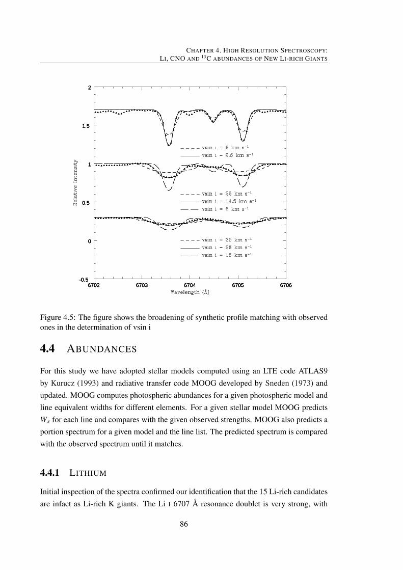
CHAPTER 4. HIGH RESOLUTION SPECTROSCOPY:LI, CNO AND 13C ABUNDANCES OF NEW LI-RICH GIANTS
6702 6703 6704 6705 6706-0.5
0
0.5
1
1.5
2
6702 6703 6704 6705 6706-0.5
0
0.5
1
1.5
2
6702 6703 6704 6705 6706-0.5
0
0.5
1
1.5
2
Figure 4.5: The figure shows the broadening of synthetic profile matching with observedones in the determination of vsin i
4.4 ABUNDANCES
For this study we have adopted stellar models computed using an LTE code ATLAS9by Kurucz (1993) and radiative transfer code MOOG developed by Sneden (1973) andupdated. MOOG computes photospheric abundances for a given photospheric model andline equivalent widths for different elements. For a given stellar model MOOG predictsWλ for each line and compares with the given observed strengths. MOOG also predicts aportion spectrum for a given model and the line list. The predicted spectrum is comparedwith the observed spectrum until it matches.
4.4.1 LITHIUM
Initial inspection of the spectra confirmed our identification that the 15 Li-rich candidatesare infact as Li-rich K giants. The Li I 6707 Å resonance doublet is very strong, with
86

4.4 ABUNDANCES
an equivalent width ranging from Wλ 100 - 600 mÅ. The resonance line is a blend ofhyperfine and possibly isotopic components. In this study, we treat the profile as purelydue to 7Li isotope which is more abundant and also stable. Li also has another transi-tion at 6103Å which is an excited line with LEP of 1.846 eV. In most cases this line isweak/absent. However, Li subordinate line at 6103 Å is measured for Li-rich K giantswhose abundances are close to cosmic value. Measured Wλ of 6707 Å and 6103 Å aregiven in Table 4.11.
6100 6102 6104 6106
0
2
4
6
8
HD77361
HD8676
HD10437
HD167304
HD37719
HD51367
HD150902
HD145457
6702 6704 6706 6708 6710
0
2
4
6
8
6100 6102 6104 6106
0
2
4
6
8
HD77361
HD8676
HD10437
HD167304
HD37719
HD51367
HD150902
HD145457
6702 6704 6706 6708 6710
0
2
4
6
8
6100 6102 6104 6106
0
2
4
6
8
HD77361
HD8676
HD10437
HD167304
HD37719
HD51367
HD150902
HD145457
6702 6704 6706 6708 6710
0
2
4
6
8
6100 6102 6104 6106
0
2
4
6
HD107484
HD118319
HD12203
HD133086
HD88476
HD40168
HD170527
6702 6704 6706 6708 6710
0
2
4
6
6100 6102 6104 6106
0
2
4
6
HD107484
HD118319
HD12203
HD133086
HD88476
HD40168
HD170527
6702 6704 6706 6708 6710
0
2
4
6
6100 6102 6104 6106
0
2
4
6
HD107484
HD118319
HD12203
HD133086
HD88476
HD40168
HD170527
6702 6704 6706 6708 6710
0
2
4
6
Figure 4.6: Spectra of new Li-rich giants showing the Li line at 6707 and 6103 .
87

CHAPTER 4. HIGH RESOLUTION SPECTROSCOPY:LI, CNO AND 13C ABUNDANCES OF NEW LI-RICH GIANTS
The spectra of program stars in the two Li profile regions are shown in Figure 4.6.The spectra of HD 77361, HD 8676, HD 10437 show very strong Li lines at 6707Å andmoderately strong 6103 Å. In some cases, the subordinate line at 6103Å is smeared outdue to high rotation. This is particularly noticeable in the spectra of HD 170527 andHD 40168 (see top left panel of Figure 4.6). Li subordinate line sits at the red wing of aFe I line. Other nearby Fe I and Ca I lines are marked (see bottom left Panel of Figure 4.6).Note subordinate line is very weak or absent in intermediate Li-rich stars.
6707 6707.5 6708 6708.5-0.5
0
0.5
1
HD 77361
6707 6707.5 6708 6708.5-0.5
0
0.5
1
HD 19745
6707 6707.5 6708 6708.5-0.5
0
0.5
1
HD 77361
6707 6707.5 6708 6708.5-0.5
0
0.5
1
HD 19745
6707 6707.5 6708 6708.5-0.5
0
0.5
1
HD 77361
6707 6707.5 6708 6708.5-0.5
0
0.5
1
HD 19745
Figure 4.7: Observed (filled triangles) and synthetic spectra (lines) around the Li I linesat 6707 Å for HD77361 and HD 19745. The computed spectra for log ε(Li) = 3.96 and3.69 matches very well with the observed spectra.
Li profile at 6707Å is quite strong and many of nearby weak lines get buried withinthe profile. For example the Fe I line at 6707Å which sits at the blue wing of the Liprofile is difficult to separate out from the main Li profile. Also, Li profile at 6707Åis blended with hyperfine and possibly isotopic components. Apart from these, numberof other weak lines of CN and atomic lines present (see Reddy et al. 2002) within thewidth of the profile which are significant in very cool spectra and where Li profile isnot strong. For these reasons, Li profile at 6707Å must be analyzed using spectrumsynthesis to derive accurate Li abundance. The wavelengths and line strengths of thesecomponents are taken from Smith et al. (1998), as corrected by Hobbs et al. (1999).
88
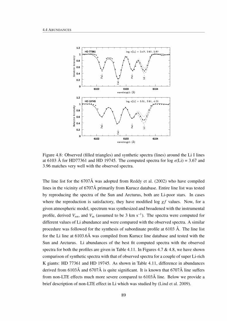
4.4 ABUNDANCES
6102 6103 61040
0.2
0.4
0.6
0.8
1
1.2
HD 77361
6102 6103 61040
0.2
0.4
0.6
0.8
1
1.2
HD 19745
6102 6103 61040
0.2
0.4
0.6
0.8
1
1.2
HD 77361
6102 6103 61040
0.2
0.4
0.6
0.8
1
1.2
HD 19745
6102 6103 61040
0.2
0.4
0.6
0.8
1
1.2
HD 77361
6102 6103 61040
0.2
0.4
0.6
0.8
1
1.2
HD 19745
Figure 4.8: Observed (filled triangles) and synthetic spectra (lines) around the Li I linesat 6103 Å for HD77361 and HD 19745. The computed spectra for log ε(Li) = 3.67 and3.96 matches very well with the observed spectra.
The line list for the 6707Å was adopted from Reddy et al. (2002) who have compiledlines in the vicinity of 6707Å primarily from Kurucz database. Entire line list was testedby reproducing the spectra of the Sun and Arcturus, both are Li-poor stars. In caseswhere the reproduction is satisfactory, they have modified log g f values. Now, for agiven atmospheric model, spectrum was synthesized and broadened with the instrumentalprofile, derived Vrot, and Vm (assumed to be 3 km s−1). The spectra were computed fordifferent values of Li abundance and were compared with the observed spectra. A similarprocedure was followed for the synthesis of subordinate profile at 6103 Å. The line listfor the Li line at 6103.6Å was compiled from Kurucz line database and tested with theSun and Arcturus. Li abundances of the best fit computed spectra with the observedspectra for both the profiles are given in Table 4.11. In Figures 4.7 & 4.8, we have showncomparison of synthetic spectra with that of observed spectra for a couple of super Li-richK giants: HD 77361 and HD 19745. As shown in Table 4.11, difference in abundancesderived from 6103Å and 6707Å is quite significant. It is known that 6707Å line suffersfrom non-LTE effects much more severe compared to 6103Å line. Below we provide abrief description of non-LTE effect in Li which was studied by (Lind et al. 2009).
89

CHAPTER 4. HIGH RESOLUTION SPECTROSCOPY:LI, CNO AND 13C ABUNDANCES OF NEW LI-RICH GIANTS
6707 6707.5 6708 6708.5-0.5
0
0.5
1
1.5
2HD 10437
HD 77361
6707 6707.5 6708 6708.5-0.5
0
0.5
1
1.5
2HD 10437
HD 77361
6707 6707.5 6708 6708.5-0.5
0
0.5
1
1.5
2HD 10437
HD 77361
6707 6707.5 6708 6708.5-0.5
0
0.5
1
1.5
2HD 10437
HD 77361
Figure 4.9: Synthetic spectra for four isotopic ratios 6Li/7Li = 0.0, 0.01, 0.03, and 0.05for two Li-rich K giants, HD 77361 and HD 10437. The 6Li/7Li = 0.0 provides the bestfit.
As noted earlier, we have made an assumption that the entire Li profiles are due tostable Li isotope which is 7Li. However, there is a possibility for the presence of someamount of 6Li. Here we investigate that possibility. The two profiles are separated byjust 0.15Å and 6Li components are at the red side of the main profile. Thus, additionof 6Li will increase the asymmetry in red side and shifts the entire profile towards red.We have computed profiles for different 6Li/7Li ratios with varying total Li abundanceand compared with the observed profiles. In all cases, our fittings showed that the profilecomputed for 6li/7li = 0.0 best matches the overall shape of the observed profile. Fittinghas been done by fixing the observed Li profile position (6707.768 ± 0.02 Å), determinedfrom the doppler shifts of symmetric Fe I and Ca I features for which accurate laboratorymeasurements are available. Within the measurement errors, the observed Li profile posi-tion matches with the predicted profile position λc = 6707.768 Å (for 7Li only). Also, theLi abundances derived with the assumption of 7Li only from 6707Å and 6103Å profilesagree very well after non-LTE correction (see Table 4.11). This is an indirect evidencethat 6Li is not present in detectable amount in any of these sample K giants.
90

4.4 ABUNDANCES
Table 4.11: Derived Lithium abundance
HDLi I 6707 Li I 6103
Wλ A(Li)LT E NLTEcorr A(Li)NLT E Wλ A(Li)LT E NLTEcorr A(Li)NLT E
77361 495 3.96 −0.16 3.80 151 3.67 0.16 3.848676 410 3.86 −0.31 3.55 86 3.46 0.14 3.6010437 405 3.76 −0.28 3.48 76 3.35 0.15 3.50
170527 360 3.31 −0.19 3.12 – 3.13 0.15 3.28167304 315 2.95 −0.098 2.852 22 2.75 0.145 2.875150902 315 2.64 0.01 2.65 18 2.56 0.17 2.7351367 320 2.58 0.02 2.60 – – – –37719 305 2.70 0.01 2.71 – – – –
145457 240 2.49 0.03 2.52 – – – –107484 238 2.04 0.10 2.14 – – – –118319 160 1.88 0.14 2.02 – – – –12203 157 2.01 0.083 2.093 – – – –
133086 145 2.03 0.116 2.146 – – – –88476 114 2.12 0.089 2.209 – – – –40168 105 1.49 0.21 1.70 – – – –
NON-LTE LI ABUNDANCES
The dominant NLTE effect is over-ionization of neutral lithium, which leads to smallnumber populations in the ground (2s) and first excited (2p) states compared to LTE andto higher values of the line source functions. Both the effects on the source functions andthe loss of line-opacity weaken the lines in non-LTE, making the abundance correctionspositive. The corrections range from being close to zero for the hottest giants to a maxi-mum of +0.45 dex for cool, metal-rich giants for the 6707Å line. For the 6103Å line, thecorrections are slightly smaller, ≤ +0.3 dex. Lind et al. (2009) computed non-LTE andLTE Li abundances for both the profiles over a wide range of Teff (4000 - 8000 K), log g
(1.0 to 5.0), [Fe/H] (0.0 to -3.0) and for Li abundance (−0.3 to 4.2 dex). They have usedLTE 1D MARCS model atmospheres with plane-parallel approximation and a radiativetransfer code (MULTI) (Carlsson 1986, 1992). The model atom in this study includes 20energy levels of neutral Li and ground state of singly ionized Li, six hyper-fine compo-nents of 7Li by neglecting 6Li for resonance line and 3 fine components for subordinateline.
In this study we have used the interpolation program provided by K.Lind (Privatecommunication). For a given set of atmospheric parameters and LTE abundance the pro-gram interpolates values provided in the Tables 2 and 3 of Lind et al. (2009) and gives the
91

CHAPTER 4. HIGH RESOLUTION SPECTROSCOPY:LI, CNO AND 13C ABUNDANCES OF NEW LI-RICH GIANTS
−0.6
−0.4
−0.2
−0.0
0.2
0.4A
(Li)
no
n−
LT
E−A
(Li)
LT
E
4500/1.0/+0.0
4500/1.0/−2.0
0 1 2 3A(Li)LTE
−0.4
−0.3
−0.2
−0.1
0.0
A(L
i)n
on
−L
TE−A
(Li)
LT
E
6000/4.5/+0.0
0 1 2 3A(Li)LTE
6000/4.5/−2.0
Figure 4.10: Non-LTE abundance corrections for 6707 Å as functions of LTE lithiumabundance for the indicated stellar parameters in the lower left corner of each plot, tobe read as Teff/ log g/[Fe/H]. S olid: Lind et al. (2009) corrections including chargetransfer reactions with hydrogen as well as bound-bound transitions due to collisions withneutral hydrogen. The cross-sections are calculated with quantum mechanics (Belyaev &Barklem 2003; Croft et al. 1999). Dotted: Carlsson et al. (1994) corrections. Dashed:Takeda & Kawanomoto (2005) corrections. Dash− dotted: Pavlenko & Magazzu (1996)
correction for LTE abundance. The recipe works for models of microturbulence of 2 km/swith solar metallicity stars. The stars in our study are close to solar metallicity but withξt from 1.3 to 1.6 km s−1. Difference of 0.5 km s−1 may not be an issue as the differencecorresponds to about 0.05 dex in the correction. The behavior of abundance corrections(non-LTE -LTE) are shown in Fig. 6. For cooler and supergiants corrections are positiveranging from 0.4 to 0.0 whereas for hotter and dwarf stars with high Li corrections arenegative. The non-LTE corrected Li abundances are given in Table 4.11.
4.4.2 Carbon, Nitrogen, and Oxygen
Our approach to find the C and N abundances was by matching computed spectrum withthe observed spectrum. Oxygen abundance was derived from equivalent widths. Forcarbon abundance, three indicators were used: the C I lines at 5380 and 5052 Å, anda C2 Swan system triplet at 5135 Å, with lower weight given to another C2 feature at5141 Å. For some stars, we also have used carbon forbidden line [C I] at 8727Å ascarbon abundance indicator. We took atomic and molecular data around the [C I] line
92

4.4 ABUNDANCES
from Gustafsson et al. (1999). For the 5380 Å line we adopted the theoretical log = -1.57 (Biemont et al. 1993). For the spectrum syntheses near 5135 Å, we took data forC2 lines from Querci, Querci, & Kunde (1971) and for MgH and the atomic lines fromthe Kurucz database. The derived carbon abundances from multiple indicators and themean abundances are given in Table 4.12. All of them are found to have mild deficient incarbon except HD 12203 ([C/Fe] = 0.16), HD 107484 ([C/Fe] = 0.02), and HD 133086([C/Fe]=0.04) .
5379.8 5380 5380.2 5380.4 5380.6
0.8
1
1.2
1.4
1.6
1.8
Sun
HD 145457
HD 77361
HD 12203
A(C) = 8.45
A(C) = 8.46
A(C) = 8.45
A(C) = 8.39
5379.8 5380 5380.2 5380.4 5380.6
0.8
1
1.2
1.4
1.6
1.8
Sun
HD 145457
HD 77361
HD 12203
A(C) = 8.45
A(C) = 8.46
A(C) = 8.45
A(C) = 8.39
5379.8 5380 5380.2 5380.4 5380.6
0.8
1
1.2
1.4
1.6
1.8
Sun
HD 145457
HD 77361
HD 12203
A(C) = 8.45
A(C) = 8.46
A(C) = 8.45
A(C) = 8.39
5379.8 5380 5380.2 5380.4 5380.6
0.8
1
1.2
1.4
1.6
1.8
Sun
HD 145457
HD 77361
HD 12203
A(C) = 8.45
A(C) = 8.46
A(C) = 8.45
A(C) = 8.39
5379.8 5380 5380.2 5380.4 5380.6
0.8
1
1.2
1.4
1.6
1.8
Sun
HD 145457
HD 77361
HD 12203
A(C) = 8.45
A(C) = 8.46
A(C) = 8.45
A(C) = 8.39
Figure 4.11: Sample spectra show the determination of Carbon abundance from the syn-thesis.
There are no detectable atomic transitions of N available in the spectra. The N I
transitions in the visible range have LEP 7-10 eV which can’t be excited in cool starssuch as K giants. Our available option is CN Red system lines at 8005 Å. Basic data forthe CN lines were taken from de Laverny & Gustafsson (1998) with a dissociation energyDo = 7.75 eV (Lambert 1994). Spectra were computed for a given carbon abundance butfor varying N abundances and we have adopted N abundance of the best fit comparison
93

CHAPTER 4. HIGH RESOLUTION SPECTROSCOPY:LI, CNO AND 13C ABUNDANCES OF NEW LI-RICH GIANTS
with the observed spectra. Derived mean N abundances are given in Table 4.12. Oxygenabundances are obtained from the [O I] 6300 Å and 6363 Å lines. Allowance was madefor a blending Ni I line Allende Prieto et al. (2001). A summary of the derived mean C,N, and O abundances and the ratios relative to Fe ([X/Fe]) are given in Table 4.12. Thesolar CNO abundances are derived in the same way as the abundances of our programstars. These are in good agreement with the solar CNO abundances found in literature(Luck & Heiter 2007).
4.4.3 The 12C/13C Ratio
The 12C/13C ratios were obtained from the CN Red system lines at 8005 Å. The CN lineat 8004.7Å is a molecule of 13C14N. Once the abundances of 14N and 12C are derived,one can obtain 12C/13C ratio from 8003Å line by varying 12C/13C ratios for fixed C and Nabundances. One needs to be cautious as the 8003 Å line is normally weak (a few mÅ)and close to telluric lines. In stars of red shifted lines, there is a possibility that theselines gets blended with weak telluric lines. We have inspected this region using Arcturusspectrum and also our own hot high rotating star spectra. In cases where we are not sureabout the contamination by the telluric lines, we have divided program spectra with thatof hot star spectra. The 12C/13C values derived from matching computing spectra withobserved spectra are given in Table 4.12. The error on the isotopic ratio was estimated asa quadratic sum of the various uncertainties. The uncertainty in C and N abundances of± 0.1 dex leads to an uncertainty of ± 2 in the 12C/13C ratio. The rms = 0.004 of the S/Nratio at the continuum yields approximately an uncertainty of 1 in the carbon ratio. Thequoted uncertainties in the derived model parameters have an insignificant effect on thederived 12C/13C ratio.
4.5 DISCUSSION AND CONCLUSIONS
Li among K giants: We confirm that all the 15 Li-rich candidate K giants identified fromour low resolution spectroscopic survey are Li-rich K giants based on high resolutionspectroscopy. We found four as super Li-rich where log ε (Li) ≥= 3.2, a value derived forISM, often referred to as cosmic Li abundance. Li abundances in the super Li-rich giantsare about a factor of 100 (or two orders of magnitude) more than the maximum expectedLi in normal K giants. Rest of the 11 giants are Li-rich with Li abundance ranging from1.7 dex to 2.9 dex about a factor of 1.5 to 25 more than the expected values. This isthe largest number of Li-rich K giants that have been found in any single study. With
94
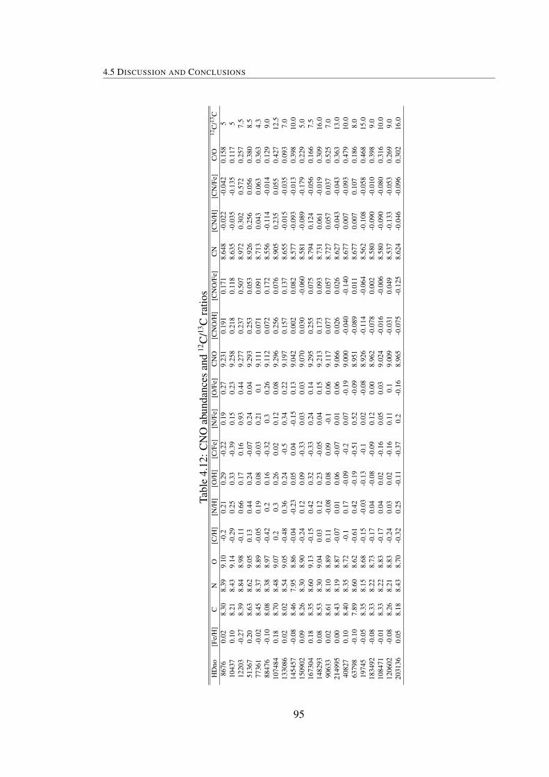
4.5 DISCUSSION AND CONCLUSIONS
Tabl
e4.
12:C
NO
abun
danc
esan
d12
C/13
Cra
tios
HD
no[F
e/H
]C
NO
[C/H
][N
/H]
[O/H
][C
/Fe]
[N/F
e][O
/Fe]
CN
O[C
NO
/H]
[CN
O/F
e]C
N[C
N/H
][C
N/F
e]C
/O12
C/13
C86
760.
028.
308.
399.
10-0
.20.
210.
29-0
.22
0.19
0.27
9.23
10.
191
0.17
18.
648
-0.0
22-0
.042
0.15
85
1043
70.
108.
218.
439.
14-0
.29
0.25
0.33
-0.3
90.
150.
239.
258
0.21
80.
118
8.63
5-0
.035
-0.1
350.
117
512
203
-0.2
78.
398.
848.
98-0
.11
0.66
0.17
0.16
0.93
0.44
9.27
70.
237
0.50
78.
972
0.30
20.
572
0.25
77.
551
367
0.20
8.63
8.62
9.05
0.13
0.44
0.24
-0.0
70.
240.
049.
293
0.25
30.
053
8.92
60.
256
0.05
60.
380
8.5
7736
1-0
.02
8.45
8.37
8.89
-0.0
50.
190.
08-0
.03
0.21
0.1
9.11
10.
071
0.09
18.
713
0.04
30.
063
0.36
34.
388
476
-0.1
08.
088.
388.
97-0
.42
0.2
0.16
-0.3
20.
30.
269.
112
0.07
20.
172
8.55
6-0
.114
-0.0
140.
129
9.0
1074
840.
188.
708.
489.
070.
20.
30.
260.
020.
120.
089.
296
0.25
60.
076
8.90
50.
235
0.05
50.
427
12.5
1330
860.
028.
028.
549.
05-0
.48
0.36
0.24
-0.5
0.34
0.22
9.19
70.
157
0.13
78.
655
-0.0
15-0
.035
0.09
37.
014
5457
-0.0
88.
467.
958.
86-0
.04
-0.2
30.
050.
04-0
.15
0.13
9.04
20.
002
0.08
28.
577
-0.0
93-0
.013
0.39
810
.015
0902
0.09
8.26
8.30
8.90
-0.2
40.
120.
09-0
.33
0.03
0.03
9.07
00.
030
-0.0
608.
581
-0.0
89-0
.179
0.22
95.
016
7304
0.18
8.35
8.60
9.13
-0.1
50.
420.
32-0
.33
0.24
0.14
9.29
50.
255
0.07
58.
794
0.12
4-0
.056
0.16
67.
514
8293
0.08
8.53
8.30
9.04
0.03
0.12
0.23
-0.0
50.
040.
159.
213
0.17
30.
093
8.73
10.
061
-0.0
190.
309
16.0
9063
30.
028.
618.
108.
890.
11-0
.08
0.08
0.09
-0.1
0.06
9.11
70.
077
0.05
78.
727
0.05
70.
037
0.52
57.
021
4995
0.00
8.43
8.19
8.87
-0.0
70.
010.
06-0
.07
0.01
0.06
9.06
60.
026
0.02
68.
627
-0.0
43-0
.043
0.36
313
.040
827
0.10
8.40
8.35
8.72
-0.1
0.17
-0.0
9-0
.20.
07-0
.19
9.00
0-0
.040
-0.1
408.
677
0.00
7-0
.093
0.47
910
.063
798
-0.1
07.
898.
608.
62-0
.61
0.42
-0.1
9-0
.51
0.52
-0.0
98.
951
-0.0
890.
011
8.67
70.
007
0.10
70.
186
8.0
1974
5-0
.05
8.35
8.15
8.68
-0.1
5-0
.03
-0.1
3-0
.10.
02-0
.08
8.92
6-0
.114
-0.0
648.
562
-0.1
08-0
.058
0.46
815
.018
3492
-0.0
88.
338.
228.
73-0
.17
0.04
-0.0
8-0
.09
0.12
0.00
8.96
2-0
.078
0.00
28.
580
-0.0
90-0
.010
0.39
89.
010
8471
-0.0
18.
338.
228.
83-0
.17
0.04
0.02
-0.1
60.
050.
039.
024
-0.0
16-0
.006
8.58
0-0
.090
-0.0
800.
316
10.0
1206
02-0
.08
8.26
8.21
8.83
-0.2
40.
030.
02-0
.16
0.11
0.1
9.00
9-0
.031
0.04
98.
537
-0.1
33-0
.053
0.26
99.
020
3136
0.05
8.18
8.43
8.70
-0.3
20.
25-0
.11
-0.3
70.
2-0
.16
8.96
5-0
.075
-0.1
258.
624
-0.0
46-0
.096
0.30
216
.0
95
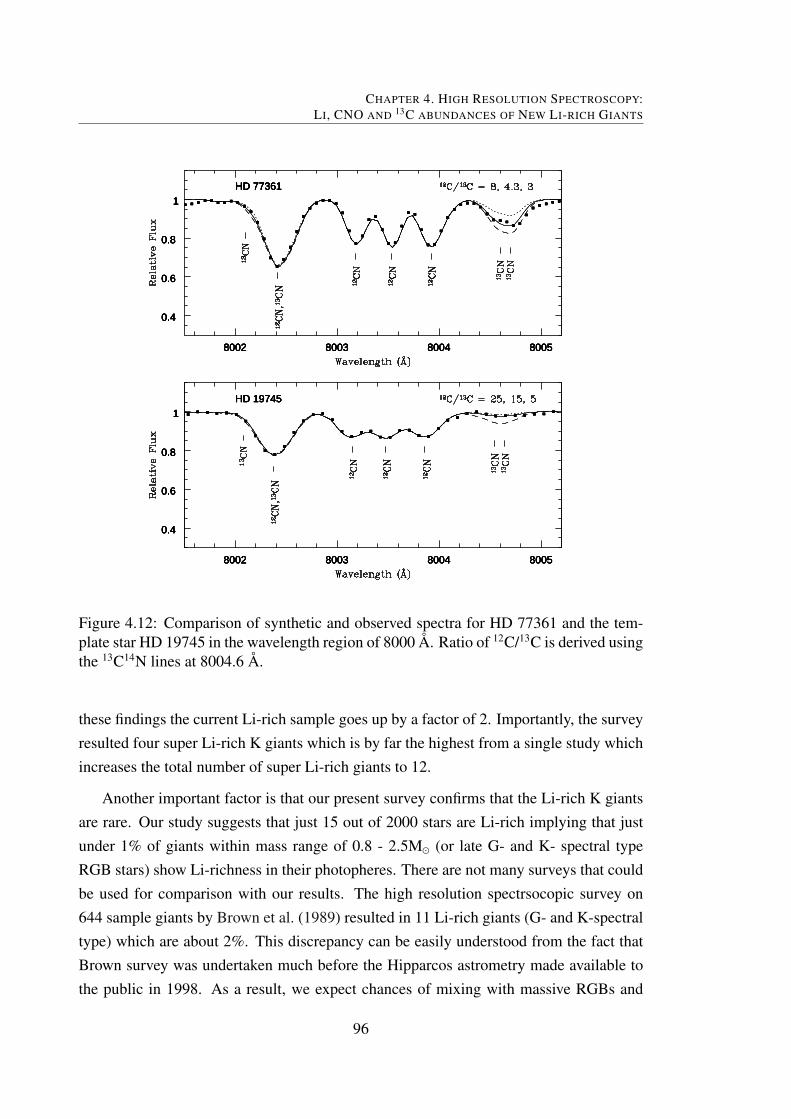
CHAPTER 4. HIGH RESOLUTION SPECTROSCOPY:LI, CNO AND 13C ABUNDANCES OF NEW LI-RICH GIANTS
8002 8003 8004 8005
0.4
0.6
0.8
1HD 77361
8002 8003 8004 8005
0.4
0.6
0.8
1HD 19745
8002 8003 8004 8005
0.4
0.6
0.8
1HD 77361
8002 8003 8004 8005
0.4
0.6
0.8
1HD 19745
8002 8003 8004 8005
0.4
0.6
0.8
1HD 77361
8002 8003 8004 8005
0.4
0.6
0.8
1HD 19745
8002 8003 8004 8005
0.4
0.6
0.8
1HD 77361
8002 8003 8004 8005
0.4
0.6
0.8
1HD 19745
8002 8003 8004 8005
0.4
0.6
0.8
1HD 77361
8002 8003 8004 8005
0.4
0.6
0.8
1HD 19745
Figure 4.12: Comparison of synthetic and observed spectra for HD 77361 and the tem-plate star HD 19745 in the wavelength region of 8000 Å. Ratio of 12C/13C is derived usingthe 13C14N lines at 8004.6 Å.
these findings the current Li-rich sample goes up by a factor of 2. Importantly, the surveyresulted four super Li-rich K giants which is by far the highest from a single study whichincreases the total number of super Li-rich giants to 12.
Another important factor is that our present survey confirms that the Li-rich K giantsare rare. Our study suggests that just 15 out of 2000 stars are Li-rich implying that justunder 1% of giants within mass range of 0.8 - 2.5M (or late G- and K- spectral typeRGB stars) show Li-richness in their photopheres. There are not many surveys that couldbe used for comparison with our results. The high resolution spectrsocopic survey on644 sample giants by Brown et al. (1989) resulted in 11 Li-rich giants (G- and K-spectraltype) which are about 2%. This discrepancy can be easily understood from the fact thatBrown survey was undertaken much before the Hipparcos astrometry made available tothe public in 1998. As a result, we expect chances of mixing with massive RGBs and
96

4.5 DISCUSSION AND CONCLUSIONS
even AGB stars in their sample is very high. To understand the discrepancy, we have re-derived luminosities and temperatures and put them in HR diagram (see Figure ??). Wefound many of their sample stars more massive and relatively more evolved on the RGBcompared to our sample. Incidences of having more Li in more massive stars (≥ 2.5M)may probably be due to insufficient mixing of original main sequence surface Li. Also,some of these stars could be early AGB stars where Li is known to be produced throughhot bottom burning (see Sackmann & Boothroyd 1999).
[Fe/H]
-0.4 -0.2 0 0.2 0.4-0.6
-0.4
-0.2
0
0.2
0.4
[Fe/H]
-0.4 -0.2 0 0.2 0.4-0.5
0
0.5
1
[Fe/H]
-0.4 -0.2 0 0.2 0.4
0
0.2
0.4
[Fe/H]
-0.4 -0.2 0 0.2 0.4-0.6
-0.4
-0.2
0
0.2
0.4
[Fe/H]
-0.4 -0.2 0 0.2 0.4-0.5
0
0.5
1
[Fe/H]
-0.4 -0.2 0 0.2 0.4
0
0.2
0.4
[Fe/H]
-0.4 -0.2 0 0.2 0.4-0.6
-0.4
-0.2
0
0.2
0.4
[Fe/H]
-0.4 -0.2 0 0.2 0.4-0.5
0
0.5
1
[Fe/H]
-0.4 -0.2 0 0.2 0.4
0
0.2
0.4
Figure 4.13: Carbon, Nitrogen,and Oxygen abundances with respect to iron abundanceare plotted against Metallicity. Filled square represents HD 12203, a thick disk giant.Open triangle represents HD 145457, planet host giant.
C,N,O abundances : Abundances of CNO and carbon isotopic ratios for the entire newLi-rich K giants are given in Table 4.12. Also, the newly derived CNO and 12C/12C ratiosfor the known Li-rich giants are given. Along with Li, CNO and carbon isotopes aresensitive, and their composition get modified as stars evolve off the main sequence toRGB and to AGB. Standard models make predictions about the effects of first dredge-
97
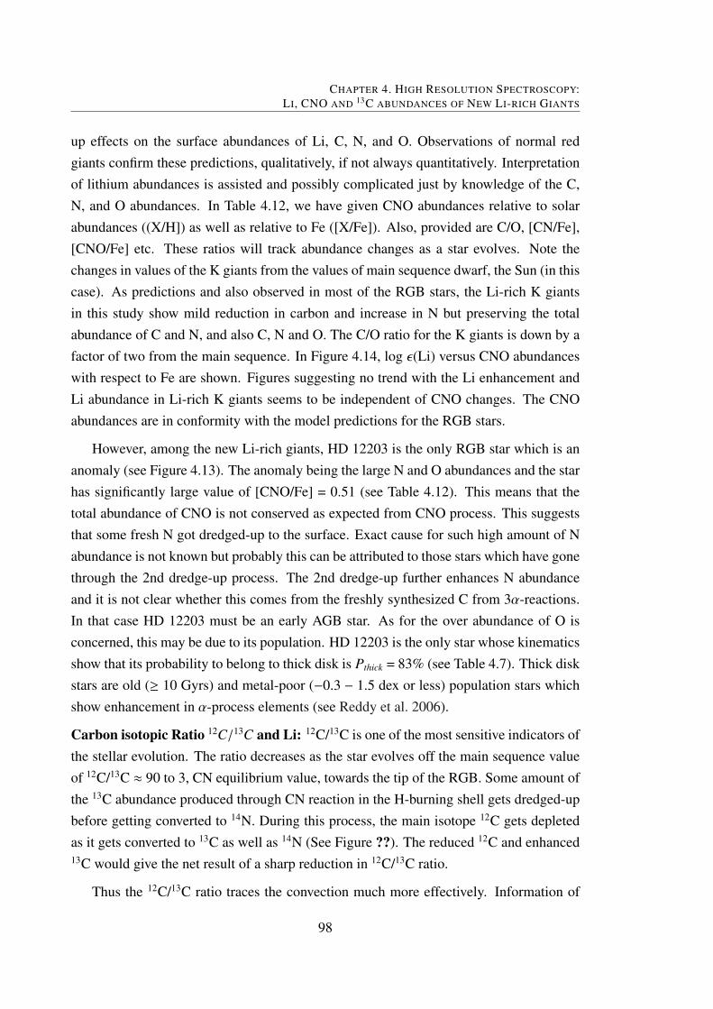
CHAPTER 4. HIGH RESOLUTION SPECTROSCOPY:LI, CNO AND 13C ABUNDANCES OF NEW LI-RICH GIANTS
up effects on the surface abundances of Li, C, N, and O. Observations of normal redgiants confirm these predictions, qualitatively, if not always quantitatively. Interpretationof lithium abundances is assisted and possibly complicated just by knowledge of the C,N, and O abundances. In Table 4.12, we have given CNO abundances relative to solarabundances ((X/H]) as well as relative to Fe ([X/Fe]). Also, provided are C/O, [CN/Fe],[CNO/Fe] etc. These ratios will track abundance changes as a star evolves. Note thechanges in values of the K giants from the values of main sequence dwarf, the Sun (in thiscase). As predictions and also observed in most of the RGB stars, the Li-rich K giantsin this study show mild reduction in carbon and increase in N but preserving the totalabundance of C and N, and also C, N and O. The C/O ratio for the K giants is down by afactor of two from the main sequence. In Figure 4.14, log ε(Li) versus CNO abundanceswith respect to Fe are shown. Figures suggesting no trend with the Li enhancement andLi abundance in Li-rich K giants seems to be independent of CNO changes. The CNOabundances are in conformity with the model predictions for the RGB stars.
However, among the new Li-rich giants, HD 12203 is the only RGB star which is ananomaly (see Figure 4.13). The anomaly being the large N and O abundances and the starhas significantly large value of [CNO/Fe] = 0.51 (see Table 4.12). This means that thetotal abundance of CNO is not conserved as expected from CNO process. This suggeststhat some fresh N got dredged-up to the surface. Exact cause for such high amount of Nabundance is not known but probably this can be attributed to those stars which have gonethrough the 2nd dredge-up process. The 2nd dredge-up further enhances N abundanceand it is not clear whether this comes from the freshly synthesized C from 3α-reactions.In that case HD 12203 must be an early AGB star. As for the over abundance of O isconcerned, this may be due to its population. HD 12203 is the only star whose kinematicsshow that its probability to belong to thick disk is Pthick = 83% (see Table 4.7). Thick diskstars are old (≥ 10 Gyrs) and metal-poor (−0.3 − 1.5 dex or less) population stars whichshow enhancement in α-process elements (see Reddy et al. 2006).
Carbon isotopic Ratio 12C/13C and Li: 12C/13C is one of the most sensitive indicators ofthe stellar evolution. The ratio decreases as the star evolves off the main sequence valueof 12C/13C ≈ 90 to 3, CN equilibrium value, towards the tip of the RGB. Some amount ofthe 13C abundance produced through CN reaction in the H-burning shell gets dredged-upbefore getting converted to 14N. During this process, the main isotope 12C gets depletedas it gets converted to 13C as well as 14N (See Figure ??). The reduced 12C and enhanced13C would give the net result of a sharp reduction in 12C/13C ratio.
Thus the 12C/13C ratio traces the convection much more effectively. Information of
98
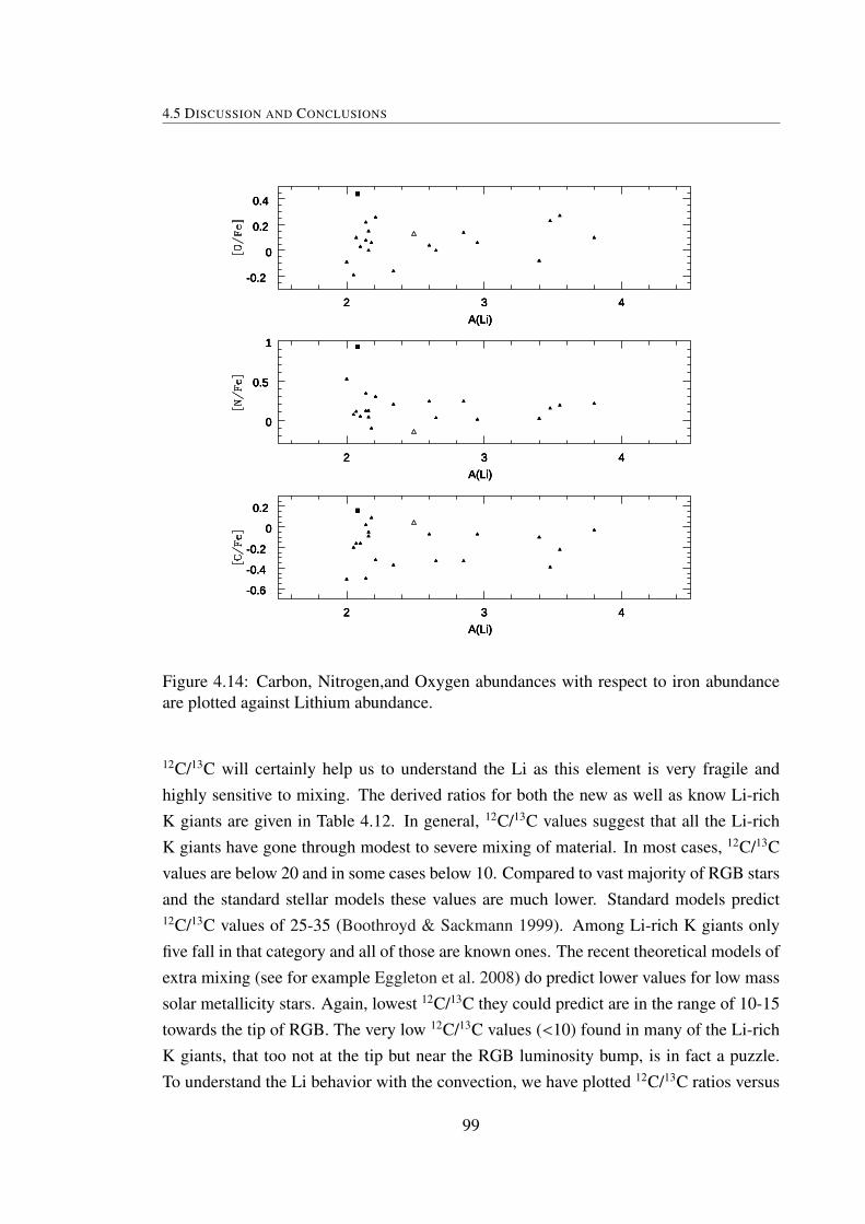
4.5 DISCUSSION AND CONCLUSIONS
A(Li)
2 3 4
-0.6
-0.4
-0.2
0
0.2
A(Li)
2 3 4
0
0.5
1
A(Li)
2 3 4
-0.2
0
0.2
0.4
A(Li)
2 3 4
-0.6
-0.4
-0.2
0
0.2
A(Li)
2 3 4
0
0.5
1
A(Li)
2 3 4
-0.2
0
0.2
0.4
A(Li)
2 3 4
-0.6
-0.4
-0.2
0
0.2
A(Li)
2 3 4
0
0.5
1
A(Li)
2 3 4
-0.2
0
0.2
0.4
A(Li)
2 3 4
-0.6
-0.4
-0.2
0
0.2
A(Li)
2 3 4
0
0.5
1
A(Li)
2 3 4
-0.2
0
0.2
0.4
Figure 4.14: Carbon, Nitrogen,and Oxygen abundances with respect to iron abundanceare plotted against Lithium abundance.
12C/13C will certainly help us to understand the Li as this element is very fragile andhighly sensitive to mixing. The derived ratios for both the new as well as know Li-richK giants are given in Table 4.12. In general, 12C/13C values suggest that all the Li-richK giants have gone through modest to severe mixing of material. In most cases, 12C/13Cvalues are below 20 and in some cases below 10. Compared to vast majority of RGB starsand the standard stellar models these values are much lower. Standard models predict12C/13C values of 25-35 (Boothroyd & Sackmann 1999). Among Li-rich K giants onlyfive fall in that category and all of those are known ones. The recent theoretical models ofextra mixing (see for example Eggleton et al. 2008) do predict lower values for low masssolar metallicity stars. Again, lowest 12C/13C they could predict are in the range of 10-15towards the tip of RGB. The very low 12C/13C values (<10) found in many of the Li-richK giants, that too not at the tip but near the RGB luminosity bump, is in fact a puzzle.To understand the Li behavior with the convection, we have plotted 12C/13C ratios versus
99

CHAPTER 4. HIGH RESOLUTION SPECTROSCOPY:LI, CNO AND 13C ABUNDANCES OF NEW LI-RICH GIANTS
1 2 3 4 5
10
20
30
A(Li)
1 2 3 4 5
10
20
30
A(Li)
1 2 3 4 5
10
20
30
A(Li)
Figure 4.15: Carbon isotopic ratios against Li abundances
Li in Figure 4.15. Red symbols represent known Li stars and the blue ones are from thisstudy. Two remarks can be made from the plot shown in Figure 4.15: a) if we considerthem as all Li-rich K giants as one group we do not see any particular trend with Lienhancement, b) All of the new Li-rich K giants show very low 12C/13C and there seemsto be a slight correlation between 12C/13C and Li abundances. In that 12C/13C graduallydecreases with steep increase in Li. Two know Li-rich K giants (HD 183492, PDS 100)also fall in this trend. More discussions on very low 12C/13C and high Li abundances aregiven in Chapter 5.
100
CHAPTER 5
SUPER LI-RICH GIANTS WITH
ANOMALOUS LOW 12C/13C RATIO
5.1 INTRODUCTION
Super Li-rich K giants are much more rare than Li-rich giants, and as of now there arejust one dozen (de La Reza & da Silva 1995; Balachandran et al. 2000; Drake et al. 2002;Reddy & Lambert 2005; Luck & Heiter 2007; Carlberg et al. 2010), including the fourbeing studied here. To understand the distribution of Li-rich stars in terms of their massand luminosity, Charbonnel & Balachandran (2000) located all the known Li-rich starson the Hertzsprung-Russell diagram, thanks to the accurate parallaxes from Hipparcos
mission (Perryman et al. 1997). The study revealed that the (M/M ≤ 2.0) super Li-rich(log ε(Li) ≥ 3.3 dex) K giants are confined to a small region on the HR diagram, the socalled luminosity bump: log L/L = 1.45 - 1.9; log Teff = 4450 - 4650 K) (Girardi et al.2000). Also, these stars are found to have lower 12C/13C ratios than the expected fromthe standard mixing theory. It is not well understood how the K giants with very deepconvective envelope and efficient mixing, as suggested from the measured low values of12C/13C, possessed such high amounts of Li; almost 10 times larger than the ISM value.In the literature, a different class of super Li-rich stars were reported. They are eithermassive (≥ 4 M) weak G- band stars (Lambert & Sawyer 1984) or AGB stars (Smith& Lambert 1989) or low mass metal-poor giants (Kraft et al. 1999; Monaco & Bonifacio2008).
The high values of Li in the super Li-rich K giants are thought to be due to the stellarnucleosynthesis and some kind of extra mixing (Denissenkov & Weiss 2000; Palacioset al. 2001; Denissenkov & Herwig 2004). At the luminosity bump on the RGB, the hy-
101

CHAPTER 5. SUPER LI-RICH GIANTS WITH ANOMALOUS LOW 12C/13C RATIO
drogen burning shell passes the µ-barrier or the mean molecular weight discontinuity thatwas created during the 1st dredge-up. This allows mixing between the cool outer layersand the hotter inner regions. This so called extra-mixing theory associated with cool bot-tom processing was invoked for Li enhancement. For low mass stars of solar metallicityat the luminosity bump, theoretical models (e.g., Denissenkov & Herwig 2004) are con-structed to match the observed peak Li abundance of log ε(Li) ≥ 3 and low 12C/13C ≈ 15 -28. The theoretical results are, in general, in agreement with the observed values of superLi-rich K giants (Charbonnel & Balachandran (2000) and references there in). As starevolves from the bump region and moves up towards the tip of RGB, Li drops sharplywith the 12C/13C ratio (Lambert et al. 1980).
The analysis of high resolution specra of new Li-rich giants resulted in four super Li-rich stars in which three are found to have anomalously low isotopic ratios of carbon, thatare close to CN equilibrium value (12C/13C ≈ 3.5). Determination of Li abundance and12C/13C ratios are discussed extensively in Chapter 4. In this chapter, we discuss high Liand low 12C/13C in these three stars along with other super Li-rich giants. We also discussthe various other stellar parameters of these giants and their location in the H-R diagram.
5.2 SUPER LI-RICH GIANTS
The three program stars, HD 77361, HD 8676, and HD 10437, are bright field stars andno previous spectroscopic analysis of either low- or high resolution spectra is available.Li-richness of these stars are idenfied from the low resolution spectra using the line depthratios of Li and nearby Ca line. The detail description of the line depth ratio technique wasdiscussed in Chapter 3. The low resolution spectra in which strong Li lines are identifiedare shown in the Figure 5.1. Later, Li-richness is confirmed by obtaining series of highresolution spectra. Figure 5.2 shows the determination of Li from the sythesis tecnique,which confirms the super Li-richess in these giants. Figure 5.3 shows the determinationof 12C/13C ratio for all these giants. Figures 5.2 & 5.3 also shown the known super Li-richK giant, HD 19745, whose Li abundance and 12C/13C are rederived similar to programstars, for comparison.
Derived atmospheric parameters, non-LTE Li abundance values, 12C/13C ratios, andvsini of the program stars along with other super Li rich stars are summarized in Table ??.Stellar masses are obtained from the evolutinary tracks. Radius is calculated from lumi-nosity and temperature. Values of projected rotational velocity (vsini) are derived fromthe synthesis of few Fe I lines (See chapter 4 for details). Luminosities are derived from
102

5.2 SUPER LI-RICH GIANTS
6550 6600 6650 67000
0.5
1
1.5
2
2.5
HD 77361
HD 8676
HD 10437
HD 170527
6550 6600 6650 67000
0.5
1
1.5
2
2.5
HD 77361
HD 8676
HD 10437
HD 170527
6550 6600 6650 67000
0.5
1
1.5
2
2.5
HD 77361
HD 8676
HD 10437
HD 170527
Figure 5.1: Detection of Strong Li line in Super Li-rich giant spectra are shown in theH-R diagram. Li and ca lines are marked
the hipparcos parallaxes and V magnitude. Few faint stars for which hipparcos parallaxesare not available, luminosities are derived from the spectroscopy. We have re-derivedLi abundance, vsini, and carbon isotopic ratios for the known sample whose spectra wereobtained along with the new Li-rich stars, also given in the same table. The values derivedby previous studies are given in bracket. For HD 214995, we have derived the 12C/13C forfirst time as no attempts so far in literature. The spectra that are not available for few faintsouthern rapid rotators, IRAS 13313-5838 (Drake et al. 2002) and G 0928+73.2600 (Carl-berg et al. 2010), for which values are taken from the original papers. Metallicity of mostof the Li-rich stars are nearby solar values except for HDE 233517 and G 0928+73.2600which are slightly metal poor (-0.3 dex). The masses of these stars are in the range of 1to 2.5 M indicates that all are low mass giants.
Figure 5.4 shows the location of super Li-rich giants in the H-R diagram. Magentasymbols are the new super Li-rich stars and blue symbols are the known ones. The loca-tion of these giants in the H-R diagram confirms that these are giants and not pre-mainsequence stars. The appearance of these giants in the HRD suggests that they are clus-tered in two different groups, cooler and hotter. A group of cool (< 4700) super Li-rich
103

CHAPTER 5. SUPER LI-RICH GIANTS WITH ANOMALOUS LOW 12C/13C RATIO
6707 6708 6709
0
2
4
HD 19745
HD 77361
HD 8676
HD 10437
HD 170527
6707 6708 6709
0
2
4
HD 19745
HD 77361
HD 8676
HD 10437
HD 170527
6707 6708 6709
0
2
4
HD 19745
HD 77361
HD 8676
HD 10437
HD 170527
6707 6708 6709
0
2
4
HD 19745
HD 77361
HD 8676
HD 10437
HD 170527
Figure 5.2: Confirmation of Li-richness in Super Li-rich giants are shown in the H-Rdiagram. Positions of 7Li and 6Li along with Fe I is marked
stars occupy near to the red kinks of evolutionary tracks. A group of hotter (> 4800)gaints are near to the black lines that are associated with the horizontal branch tracks.
5.3 DISCUSSION AND CONCLUSION
For the most Li-rich K giant HDE 233517 and new super Li-rich giant HD 170527, un-fortunately, the 12C/13C ratio is not available, probably, due to its very high rotation ofvsini = 17 km s−1 and 25 km s−1, respectively. Generally, the 13C14N lines at 8004.6 Å,often used for the carbon isotopic ratio, is weak and gets smeared out in the spectra ofhigh rotation stars. It is clear from the Table that these giants have a range of projectedrotational velocities and isotopic ratios. Seven out of twelve are moderately high rotators(≥ 5 km s−1) and remaining are slow rotators similar to normal giants (≤ 3 km s−1). Notethe rapid rotators have significantly higher 12C/13C.
It is clear from the Table 5.1 that HD 77361 is a super Li-rich, and the 3rd most Li-rich K giant amongst twelve super Li-rich K giants known so far. The derived luminosity(log(L/L) = 1.66) and Teff = 4580 K places HD 77361 at the RGB luminosity bump.
104

5.3 DISCUSSION AND CONCLUSION
8002 8003 8004 8005
0.5
1
1.5
2
HD 19745
HD 77361
HD 8676
HD 10437
8002 8003 8004 8005
0.5
1
1.5
2
HD 19745
HD 77361
HD 8676
HD 10437
8002 8003 8004 8005
0.5
1
1.5
2
HD 19745
HD 77361
HD 8676
HD 10437
8002 8003 8004 8005
0.5
1
1.5
2
HD 19745
HD 77361
HD 8676
HD 10437
Figure 5.3: Determination of 12C/13C of new super Li-rich giants are shown along withthe Known sample,HD 19745, for comparison.
The most striking from the results shown in Table 5.1 is that the lowest 12C/13C ratioof HD 77361 among all super Li-rich giants. The other super Li-rich stars have signifi-cantly higher values of 12C/13C ratios except HD 8676 and HD 10437. It is puzzling thatHD 77361 has a 12C/13C ratio that is close to the CN equilibrium value, but continues tohave peak value of Li on its surface. Another important point to be noticed is that thelocation of super Li-rich stars in the H-R diagram. The group of cool super Li-rich starsare very close to the expected luminosity bump region for a given stellar mass. Results ofHD 77361 strengthens the argument that the changes to the stellar structure of low massstars at the bump region are the main cause for the sudden reduction in 12C/13C ratio, andthe enhancement of Li on the surface of first ascend giant branch stars.
5.3.1 LI AND 12C/13C AT THE RGB BUMP
It is known that at the RGB bump the hydrogen burning shell moves past the so called µ-barrier. In the absence of µ-barrier, convective zone reaches much deeper level dredgingup the hydrogen burning products to the surface altering abundances of Li, C, N, and 13Cmuch more severely compared to the predictions of standard 1st dredge-up scenario. This
105

CHAPTER 5. SUPER LI-RICH GIANTS WITH ANOMALOUS LOW 12C/13C RATIO
Tabl
e5.
1:V
alue
sof
stel
larp
aram
eter
s(M
etal
licity
,Teff
,Mas
s,lu
min
osity
)and
the
surf
ace
abun
danc
esva
lues
oflo
gε(
Li)
and
carb
onis
otop
icra
tios
ofsu
perL
i-ri
chK
gian
ts.
Star
[Fe/
H]
Teff
M?
/M
log
L/L
R?
/R
logε(
Li)
12C
/13C
Vsi
niH
D77
361
−0.
0245
801.
51.
6610
.75
3.82
4.3±
13
HD
8676
0.00
4860
2.4
1.67
9.66
3.58
5.0±
13
HD
1043
70.
0548
302.
51.
7710
.97
3.49
5±
13
HD
1705
27...
4811
2.3
1.69
10.1
13.
20...
25H
D23
3517
−0.
3744
751.
72.
0a16
.66
4.22
...17
.6IR
AS
1353
9-41
53−
0.13
4300
0.8
1.60
a11
.38
4.05
205
HD
9746
−0.
0644
001.
922.
0217
.64
3.75
24(2
8±4)
8.7
HD
1974
5−
0.05
4700
2.2
1.90
a13
.46
3.70
15(1
6±2)
2H
D19
4937
−0.
0148
631.
731.
573.
41...
1.0
IRA
S13
313-
5838
−0.
0945
401.
11.
85a
13.6
23.
312
+8−
220
HD
2149
95−
0.00
4737
1.80
1.54
3.28
134.
5G
0928
+73.
2600
−0.
2548
851.
753.
3028±
88.
4a H
ippa
rcos
astr
omet
ryis
nota
vaila
ble
and
valu
esof
lum
inos
ities
and
mas
ses
are
deriv
edfr
omsp
ectr
osco
py.
106

5.3 DISCUSSION AND CONCLUSION
5500 5000 4500 4000
0.5
1
1.5
2
2.5
[Fe/H] = 0.0
5500 5000 4500 4000
0.5
1
1.5
2
2.5
[Fe/H] = 0.0
5500 5000 4500 4000
0.5
1
1.5
2
2.5
[Fe/H] = 0.0
5500 5000 4500 4000
0.5
1
1.5
2
2.5
[Fe/H] = 0.0
Figure 5.4: Super Li-rich giants are shown in the H-R diagram. Blue and magenta sym-bols are known and new sample giants, respectively.
is known as extra mixing (Sweigart & Mengel 1979; Charbonnel et al. 1998) which isdifferent from the ordinary convective mixing. The extra mixing is invoked to explainthe observed, in general, low values of Li and 12C/13C ratio at or above the RGB bump(Lambert et al. 1980; Gratton et al. 2000). The exact mechanism for the extra mixing isstill an issue to be worked out.
For the Population I stars of low mass (M/M ≤ 2.5) theoretical models of extra mix-ing predict final 12C/13C ratios as low as 10 when star evolves to the RGB tip. Boothroyd& Sackmann (1999) demonstrated that deep circulation mixing at the base of convectiveenvelope and the associated cool bottom processing brings down the 1st dredge-up pre-diction of 12C/13C ≈ 28 to the lowest final value of 10 closer to the RGB tip for a starof 1.5 M with solar metallicity. Similar results from the recent computations based onenhanced extra mixing triggered by external sources (Denissenkov & Herwig 2004) andmean molecular weight inversion or δ-mixing (Eggleton et al. 2008) predicted final values
107

CHAPTER 5. SUPER LI-RICH GIANTS WITH ANOMALOUS LOW 12C/13C RATIO
of 12C/13C ≈ 10-14 for low mass Pop I stars. However, in all the models, stars at the RGBbump region are expected to have 12C/13C ratios at about 15 or more.
Earlier suggestions of planet or dwarf companion merger (Alexander 1967; Brownet al. 1989; Siess & Livio 1999) with the parent stars or addition of Li rich material fromthe nearby novae ejections (Gratton & D’Antona 1989) cannot explain the localization ofsuper Li-rich stars on the HR diagram. If the Li enhancement in the K giant is due to theexternal sources like planet engulfment or accretion of novae material, it could happenanywhere on the RGB phase. Absence of low mass super Li-rich giants below or abovethe RGB bump simply means that Li enhancement is related to changes in the internalstellar structure and the mixing process that are associated with the luminosity bump.Depletion of Li starts once again, from the peak Li abundance at the RGB bump, as starsevolve towards the RGB tip. Observations show, in general, very low Li abundances (logε(Li) = −1.0 - 1.5 dex) in K giants between the bump and the RGB tip. As discussedby de La Reza et al. (1997) and calculated by Denissenkov & Herwig (2004) the superLi-rich phase on the RGB seems to be very short (a few million years), and all the lowmass stars, perhaps, experience this phase.
Another suggestion one can infer from the results shown in Table 2 is that the absenceof correlation between Li enhancement and the 12C/13C ratio at the bump. It seems Lienhancement in the K giants at the bump is independent of the 12C/13C ratio, and hencelongevity or the extent of the deep mixing process. Sackmann & Boothroyd (1999) sug-gest that Li can be enhanced on the surface as long as fast deep mixing is ensured, andin fact they have predicted high values of Li towards the RGB tip (not at the RGB bump)where 12C/13C values are low. On the other hand, Palacios et al. (2001) hypothesizedthat the surface 7Li enhancement is the precursor for the extra mixing. Given the verylow value of 12C/13C ratio for the HD 77361, one may suggest that erasing the µ-barrier,and hence the free mixing of material between hydrogen burning shell and the bottom ofconvective outer layer seems to be providing conducive environment for the enhancementof surface Li abundance.
It is understood that Li is produced in the inner layers of the stars through Cameron& Fowler (1971) mechanism. Sustaining the Li production and dredging up the Li richmaterial to outer layers to the observed levels is still an unsolved problem. For safe trans-portation of 7Be produced in the inner layers via 3He(α, γ)7Be to cooler regions, so that7Li could be produced and mixed up with the photosphere, a few possibilities were ex-plored. Palacios et al. (2001) suggested Li-flash scenario for high Li-abundance. In thisscenario, 7Be diffuses outward where Li can be produced via 7Be(e−, ν)7Li and forms the
108

5.3 DISCUSSION AND CONCLUSION
so called Lithium burning shell. Energy release from the destruction of 7Li by proton aswell as from production of 7Li destabilize the Li burning shell leading to runway situa-tion. This in turn leads to the enhanced meridional circulation and hence the observedLi enhancements. In this scenario Li enhancement precedes the 12C/13C reduction. Thisexplains the localization of super Li-rich K giants at the bump and also the relativelyhigh values of carbon isotopic ratios (Charbonnel & Balachandran 2000). As K giantsevolve away from the bump Li starts decreasing with the decreasing 12C/13C ratio. Atotally different approach was suggested from the computations by Denissenkov & Her-wig (2004). An enhanced extra mixing triggered by spinning up of the K giants withthe external angular momentum can produce the required mixing coefficients. Source ofthe external angular momentum could be either by the synchronization of K giant’s spinwith the orbital motion of close binary or engulfment of massive planet. This mechanismwill enhance K giant’s angular momentum by 10-fold, and explains high rotation velocityobserved in some of the Li-rich K giants. But, as stated earlier, fails to explain the pres-ence of all the twelve super Li-rich at the bump and the absence of super Li-rich stars anywhere along the RGB path. In all of these models, Li peak was achieved when the 12C/13Cratios are around 15 - 28 which are in general agreement with the six of the twelve superLi-rich stars shown in the Table 5.1.
109


CHAPTER 6
INFRARED EXCESS VS LITHIUM
6.1 INTRODUCTION
Low mass K giants are known to loose mass through stellar winds which are driven bystellar radiation. Mass-loss creates circumstellar dust around stars which absorbs part ofstar’s radiation in visual wavelengths and re-emits in longer wavelengths. This is seen asinfrared (IR) excess (Zuckerman et al. 1995). The connection between Li enhancement inK giants and the IR excess was first discussed by Gregorio-Hetem et al. (1993) based onthe results obtained from the survey called Pico Dias Survey (hereafter PDS) which wasoriginally meant for searching T-Tauri stars using far-IR color criteria. The survey led todiscover a couple of Li-rich K giants whose IR colors overlapped with those of T-Tauristars. The so called connection between IR excess and the high Li in K giants promptedmore surveys to look for new Li-rich K giants based on IRAS color criteria (Gregorio-Hetem et al. 1993; de La Reza et al. 1997; Castilho et al. 1998). The number of K giantswith IR excess obviously increased partly due to the bias in the criteria.
However, there are K giants with large Li but without IR excess, and K giants withsignificant IR excess but with normal Li. In the literature, there are many models con-necting the Li-enhancement with the infrared excess. For example, the model developedby de La Reza et al. (1996) supported such a relation between Li enhancement and IRexcess, and the observed IR excess is interpreted as due to expanding dust shell. Themodel suggest that all the normal K giants become Li-rich during a short interval of afew thousand years during the RGB phase, and the RGB phase lasts for about a few tensof million years. Various models were developed to understand the underlying physicalprocess that are responsible to create excess as well as Li. Palacios et al. (2001) studyprovided a mechanism for such a scenario where rotation-induced mixing would cause
111
CHAPTER 6. INFRARED EXCESS VS LITHIUM
Li-enhancement as well as increase in mass-loss at the luminosity bump due to thermalinstability in the lithium burning shell which they called as Li flash. Another interestingmodel was by Denissenkov & Herwig (2004) who proposed the Li enrichment due toenhanced extra mixing triggered by an external source like plunging of massive planetsor a brown dwarf. According to them, the IR excess can be due to an orbiting dusty diskformed due to planet engulfment (e.g; Jura 2003) instead of an expanding dust shell.
However, the above models and observational inferences are based on a handful num-ber of Li-rich K giants. To draw meaningful conclusions we require a study of substantialnumber of K giants with or without Li as well as K giants with or without IR-excess. Inthis chapter, we aim to study the infrared properties of a large number of K giants alongthe red giant branch. The data of excess of IR radiation was from IRAS measurements.The mass-loss rates were derived by modeling their spectral energy distribution (SED)using a radiative transfer code DUSTY. Using this approach, we have investigated therelation between Li enhancement and mass-loss for the first time for such a large sample.
6.2 SAMPLE SELECTION
The sample for our study consists of 2000 low mass (0.8 to 3.0 M) normal giants and theupdated list of Li-rich giants. Normal giants are the survey sample taken from Chapter 3and the entire list of Li-rich giants are taken from Chapter 4. Selected candidates occupythe RGB track beginning from the base of the RGB to beyond the post luminosity bump.The entire sample is divided into four bins in the HR diagram based on temperature, lumi-nosity, and mass. The four bins are the pre-bump, bump, clump and post-bump. Samplestars with superposed evolutionary tracks are shown in Figure 6.1. Solid blue lines areevolutionary tracks for 0.8 to 3.0 M stars computed for solar metalliciy, [Fe/H]=0.0(Bertelli et al. 2008). Red dashed lines represent the base of RGB where the convectiveenvelope deepens to a maximum extent. Red solid lines are the kinks in luminosity rep-resenting the amplitude of the luminosity bump or known as RGB bump. Yellow solidlines represent the red clump, where post He-core flash objects settle. These are core Heburning stars. Cross symbols are the Li-normal giants, whose Li abundances, derived inthis study from low resolution spectra (see Chapter 3), are below 1.4 dex. Green, cyan,black, and magenta crosses are pre-bump, bump, clump and post-bump giants, respec-tively. Obviously, the number of giants are relatively large in bump and clump regions.Blue filled circles are Li-rich K giants, whose Li abundances were derived from the highresolution spectral analysis (see Chapter 4 for details). The size of the circle represents
112

6.3 INFRARED EXCESS
5500 5000 4500
0.5
1
1.5
2
2.5
5500 5000 4500
0.5
1
1.5
2
2.5
5500 5000 4500
0.5
1
1.5
2
2.5
5500 5000 4500
0.5
1
1.5
2
2.5
Figure 6.1: Li-rich and normal K giants are on the HR-diagram. Evolutionary tracks forlow mass (0.8 - 3M) stars are superposed. Blue circles represents the Li-rich K giantsand the size indicates the relative amount of lithium. Green, black, cyan, and magentacrosses represent pre-bump, red clump, bump, and post-bump giants, respectively.
the amount of Li. We find all the Li-rich K giants in the bins of bump and clump, andnone in the other two bins of pre-bump and post-bump.
6.3 INFRARED EXCESS
Excess infrared radiation from a star indicates the presence of circumstellar dust. Thehot and warm dust emits in near-infrared (NIR) wavelengths and cooler dust emits infar-infrared (FIR) wavelengths. Color-Color diagram (CCDm) is one of the tools oftenused in astronomy to study the excess radiation coming from a star. The diagram consistsof color indices in both the axes. Color indices between two bands are derived from theintrinsic magnitudes at the two bands. As the star light passes through the interstellar
113

CHAPTER 6. INFRARED EXCESS VS LITHIUM
matter, the observed color needs to be corrected for interstellar reddening to get the in-trinsic color of the star. The entire sample stars are checked for the existence of excess inNIR and FIR wavelengths.
6.3.1 NEAR-INFRARED CCDM
NIR CCDm helps to detect the warm and hot dust in the circumstellar orbiting disks andexpanding shells. The typical colors used in NIR studies are (J-H) and (H-K). We havetaken the NIR magnitudes in J, H, and Ks for the entire sample of stars from 2MASScatalog (Cutri et al. 2003). The quality of the data in the catalog varies from good toupperlimits. The sample consists of cooler red giants, so most of them have upperlimitfluxes in Ks band. Observed (J-H) and (H-K) colors are converted into the Koornneef
-0.5 0 0.50
0.2
0.4
0.6
0.8
1
1.2
-0.5 0 0.50
0.2
0.4
0.6
0.8
1
1.2
-0.5 0 0.50
0.2
0.4
0.6
0.8
1
1.2
-0.2 0 0.2 0.4 0.6 0.8 1
0
0.5
1
-0.2 0 0.2 0.4 0.6 0.8 1
0
0.5
1
-0.2 0 0.2 0.4 0.6 0.8 1
0
0.5
1
-0.2 0 0.2 0.4 0.6 0.8 1
0
0.5
1
Figure 6.2: Li-rich and Li-normal giants are on Near IR color-color diagram.
(1983) system using transformation relations given in Carpenter (2001). The locationof main-sequence (MS) stars, giants, and reddening vector in the NIR CCDm are takenfrom (Koornneef 1983). NIR colors with the error bars of Li-rich giants are plotted in NIRCCDm in the left panel of Figure 6.2 and the Li-normal giants are plotted in right panel.Red circles are Li-rich giants and blue open triangles are Li-normal giants. The dashedline indicates the reddening vector. Black solid line is the location of dwarfs. Green lineindicates the location of giants. Many of the giants are well inside the reddening vector,indicating that no excess emission is found in NIR. The stars which are falling left side on
114

6.3 INFRARED EXCESS
the diagram is due to large errors in the magnitudes. A few of them are having excess. Werestrict our NIR study here to find the excess from CCDm. A detail study using spectraenergy distribution (SED) will be discussed later in this chapter.
6.3.2 FAR-INFRARED CCDM
The excess radiation in FIR from the star indicates the presence of cool circumstellar dust,which can be detected using FIR CCDm. The colors, [12-25] and [25-60], used in the FIRCCDm are based on the IRAS fluxes at 12µ, 25µ, and 60µ bands and using Equation 6.1.The general definition to calculate colors for λ1 and λ2 are :
[λ1 − λ2] = logλ2 fλ1 − logλ1 fλ2 (6.1)
where λ1 and λ2 are the central wavelength of the bands 1 and 2, fλ1 and fλ2 are thefluxes at λ1 and λ2, respectively.
IRAS fluxes along with the quality code of the data and calculated colors of Li-richgiants are given in Table 6.1 . The location of Li-rich K giants are shown on IRAS color-color diagram (see Figure 6.3). The quality of the data in this catalog varies from good,moderate, and upper limits. The quality of the data are shown in red, blue, and blacksymbols for good, moderate and upper limits, respectively. The size of open hexagonsrepresents the amount of Li. Red square is Arcturus, a typical K giant with very low Li(A(Li)∼-0.6) and no infrared excess, which is shown for reference. There are three re-gions seen in the diagram and are named as region I, region II, and region III. The starsin the region I do not show 25µ and 60µ excesses indicating the absence of circumstellardust. For these stars, the dust might not have formed or it might have formed and dissi-pated into interstellar space. The region II is where the star shows excess in both 25µ and60µ indicating clearly the presence of a warmer and extended dust. Region III is wherethe excess is seen only at 60µ indicating the presence of an extended cool dust shell. Inthe diagram, Li-rich giants are showing excess emission either in 25µ or 60µ, indicatingthe presence of a dusty region around the central star. However, the quality of fluxes areupperlimits for a few candidates. The position of the giants in the diagram whose upper-limit fluxes at only 60µ will come vertically down and the objects with upperlimit fluxesat both 25µ and 60µ will come down diagonally. This indicates that they are associatedwith lesser excess in 60µ than the present estimation.
FIR colors also derived for prebump, bump, clump and post-bump giants. Most of the60 µ fluxes and significant number of 25µ fluxes have upper limits. Prebump giants have
115

CHAPTER 6. INFRARED EXCESS VS LITHIUM
Table 6.1: IRAS fluxes of Li-rich giants from IPAC 1986Star F12 Qual F25 Qual F60 Qual F100 Qual [25-12] [60-25]
Jy Jy Jy JyHD108471 0.869 3 0.361 1 0.4 1 1 1 -0.700 -0.335HD118319 1.04 3 0.287 1 0.4 1 1 1 -0.877 -0.236HD120602 1.129 3 0.278 1 0.4 1 1 1 -0.927 -0.222HD12203 0.793 3 0.409 1 0.4 1 1 1 -0.606 -0.389HD133086 0.706 3 0.25 1 0.4 1 1 1 -0.769 -0.176HD203251 0.416 3 0.369 1 0.4 1 1 1 -0.370 -0.345HD217352 0.701 3 0.308 1 0.4 1 1 1 -0.675 -0.266HD63798 0.865 3 0.347 1 0.4 1 1 1 -0.715 -0.318HD88476 0.638 3 0.29 1 0.4 1 1 1 -0.661 -0.240HD21018 0.859 3 0.285 1 0.4 1 1.01 1 -0.797 -0.232HD150902 0.298 3 0.25 1 0.4 1 1.07 1 -0.396 -0.176HD37719 0.376 3 0.25 1 0.4 1 1.37 1 -0.496 -0.176HD40168 0.759 3 0.25 1 0.4 1 2.33 1 -0.801 -0.176HD203136 0.444 3 0.305 1 0.584 1 22.6 1 -0.482 -0.098HD112127 0.979 3 0.290 2 0.4 1 1 1 -0.846 -0.241HD31993 0.785 3 0.291 2 0.4 1 1 1 -0.748 -0.243HD40827 1.51 3 0.368 2 0.4 1 1 1 -0.931 -0.343HD170527 0.873 3 0.264 2 0.4 1 1.02 1 -0.837 -0.200HD51367 0.705 3 0.246 2 0.4 1 5.22 1 -0.774 -0.170HD10437 1.12 3 0.304 2 0.4 1 8.38 1 -0.884 -0.261HD145457 0.988 3 0.316 3 0.4 1 1 1 -0.813 -0.278HD167304 1.28 3 0.281 3 0.4 1 1 1 -0.977 -0.226HD214995 1.84 3 0.438 3 0.4 1 1 1 -0.942 -0.419HD90633 1.41 3 0.346 3 0.4 1 1 1 -0.928 -0.317HD148293 3.52 3 0.78744 3 0.4 1 1.47 1 -0.969 -0.674HD116292 2.51 3 0.661 3 0.4 1 1.97 1 -0.898 -0.598HD9746 2.74 3 0.712 3 0.4 1 4.38 1 -0.904 -0.630HD77361 1.58 3 0.427 3 0.4 1 5.12 1 -0.886 -0.408HD214714 1.12 3 0.314 3 0.4 1 6.12 1 -0.870 -0.275HD205349 6.75 3 1.68 3 0.419 1 3.36 1 -0.922 -0.983HD787 9.33 3 2.37 3 0.485 1 1 1 -0.913 -1.069IRAS17596-3952 0.482 3 1.11 2 0.637 2 12.7 1 0.044 -0.621HD19745 0.332 3 0.777 3 0.612 3 1 1 0.050 -0.483IRAS13539-4153 0.491 3 0.821 3 0.644 3 1 1 -0.095 -0.485HD146850 6.91 3 1.78 3 1.93 3 5.99 2 -0.907 -0.345IRAS13313-5838 1.88 3 6.04 3 3.3 2 22.5 1 0.188 -0.642PDS100 4.74 3 6.53 3 3.38 3 10.6 1 -0.179 -0.666HD219025 17.1 3 10.3 3 3.86 3 1.7 3 -0.538 -0.806HD233517 0.502 3 3.6 3 7.6 3 5.1 3 0.536 -0.0551 = Upper limits; 2 = Moderate; 3 = High
more data with upperlimits in 25µ and 60µ than other giants, implying that these starsdo not emit strongly in far-infrared. The giants in all the 4 bins are Li-normal. For ouranalysis, we considered the sources with good and moderate quality of fluxes in all theIRAS bands to derive their IR properties. Li-normal and Li-rich giants with only goodand moderate quality of data are shown in IRAS color-color diagram (see Figure 6.4).
116

6.3 INFRARED EXCESS
-1 -0.5 0 0.5
-1
-0.5
0
I
II
III
-1 -0.5 0 0.5
-1
-0.5
0
I
II
III
-1 -0.5 0 0.5
-1
-0.5
0
I
II
III
Figure 6.3: Location of Li-rich giants on the far infrared color-color diagram. Trianglesare the Li-rich giants. Size of the open hexagons represents the relative amount of lithium,1.4 ≤ A(Li) < 2.0, 2.0 ≤ A(Li) < 2.5, 2.5 ≤ A(Li) < 3.3, and A(Li) ≥ 3.3, respectively.Red square is the Arcturus, a typical K giant with A(Li) < 0.0 . Black color indicates theupper limits of fluxes at 25µ and 60µ. Blue color is for the upper limit flux at 60µ. Redcolor is for the high and moderate quality fluxes at 12, 25, and 60µ
Red filled triangles are Li-rich giants and open symbols are Li-normal giants. Triangles,squares, pentagons, and hexagons represent pre-bump, bump, clump, and postbump gi-ants respectively. In the diagram, most of the Li-normal giants are in the region wherethere is no excess in colors indicating the absence or negligible amount of circumstellardust. A few of them are showing more excess in 60µ. Only a little fraction of giants areshowing excess in both 25µ and 60µ bands.
The above analysis suggests that most of the Li-rich giants and a few Li-normal giantsare associated with the circumstellar dust and the giants which are associated with theinfrared excess are occupying the regions which are at or above the bump and the clumpluminosity in the HR diagram. Most of the Li-normal giants are occupying the region I,indicating that the normal giants, in general, are not associated with infrared excess. Afew Li-normal giants at region III (bump, clump and post-bump) have extended cool dust,which may be due to additional mass-loss encountered on the RGB. Li-rich giants in thebump and clump region in the HR diagram are located in region II in the FIR CCDm,which indicates more excess compared to normal giants.
117

CHAPTER 6. INFRARED EXCESS VS LITHIUM
-1 -0.5 0 0.5-1.5
-1
-0.5
0
-1 -0.5 0 0.5-1.5
-1
-0.5
0
-1 -0.5 0 0.5-1.5
-1
-0.5
0
-1 -0.5 0 0.5-1.5
-1
-0.5
0
-1 -0.5 0 0.5-1.5
-1
-0.5
0
-1 -0.5 0 0.5-1.5
-1
-0.5
0
-1 -0.5 0 0.5-1.5
-1
-0.5
0
-1 -0.5 0 0.5-1.5
-1
-0.5
0
Figure 6.4: Li-rich and normal giants with only good quality of data are presented. Filledtriangles are the Li-rich K giants. Open symbols are normal giants. Triangles, squares,pentagons and hexagons represent pre-bump, bump,clump, and postbump, respectively
6.4 GEOMETRY OF THE CIRCUMSTELLAR DUST
The geometrical distribution of dust around a star, spherical or non-spherical, gives aninformation regarding the origin of the dust formation. The geometry of the dusty regionaround the sample giants can be obtained using the dust emissivity index (α). For a dustcloud of uniform temperature, the ratio of emitted flux at two wavelengths λ1 and λ2 inthe optically thin limit is
Fλ1
Fλ2
=
(λ2
λ1
)α Bλ1(Td)Bλ2(Td)
(6.2)
where α is the dust opacity index and Bλ(Td) is the Planck’s function at λ for dust tem-perature Td.
Bλ(Td) =2hcλ3
(1
ehc
kλTd − 1
)(6.3)
Flux ratios, (F12/F25) and (F25/F60), are calculated from the moderate and good quality offluxes at 12µ, 25µ, and 60µ bands of IRAS. Dust temperature (Td) and dust opacity index(α) are obtained simultaneously by fitting flux ratios (F12/F25) and (F25/F60) described inabove equations and shown in Figure 6.5.
The equations used in this analysis are adopted from Muthumariappan et al. (2006)
118
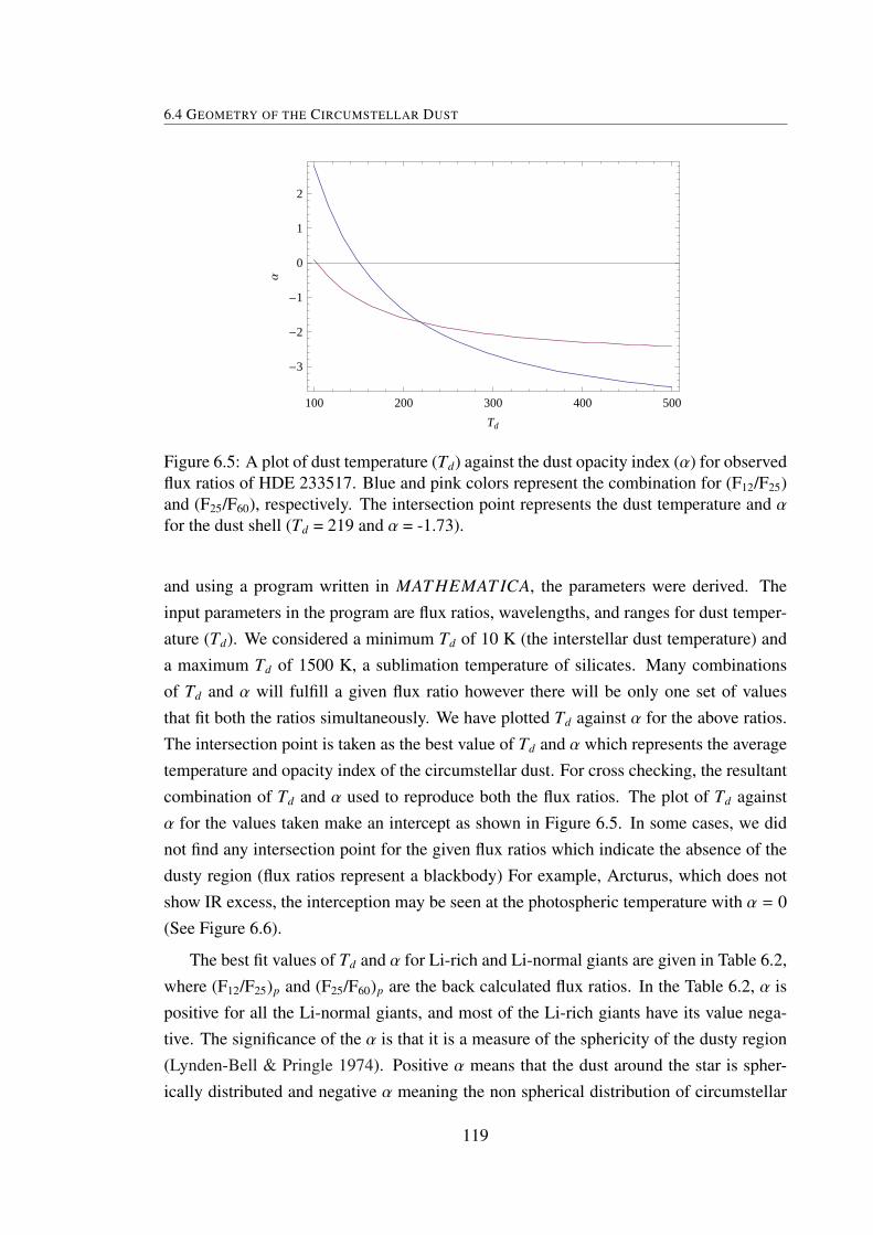
6.4 GEOMETRY OF THE CIRCUMSTELLAR DUST
100 200 300 400 500
-3
-2
-1
0
1
2
Td
Α
Figure 6.5: A plot of dust temperature (Td) against the dust opacity index (α) for observedflux ratios of HDE 233517. Blue and pink colors represent the combination for (F12/F25)and (F25/F60), respectively. The intersection point represents the dust temperature and αfor the dust shell (Td = 219 and α = -1.73).
and using a program written in MAT HEMAT ICA, the parameters were derived. Theinput parameters in the program are flux ratios, wavelengths, and ranges for dust temper-ature (Td). We considered a minimum Td of 10 K (the interstellar dust temperature) anda maximum Td of 1500 K, a sublimation temperature of silicates. Many combinationsof Td and α will fulfill a given flux ratio however there will be only one set of valuesthat fit both the ratios simultaneously. We have plotted Td against α for the above ratios.The intersection point is taken as the best value of Td and α which represents the averagetemperature and opacity index of the circumstellar dust. For cross checking, the resultantcombination of Td and α used to reproduce both the flux ratios. The plot of Td againstα for the values taken make an intercept as shown in Figure 6.5. In some cases, we didnot find any intersection point for the given flux ratios which indicate the absence of thedusty region (flux ratios represent a blackbody) For example, Arcturus, which does notshow IR excess, the interception may be seen at the photospheric temperature with α = 0(See Figure 6.6).
The best fit values of Td and α for Li-rich and Li-normal giants are given in Table 6.2,where (F12/F25)p and (F25/F60)p are the back calculated flux ratios. In the Table 6.2, α ispositive for all the Li-normal giants, and most of the Li-rich giants have its value nega-tive. The significance of the α is that it is a measure of the sphericity of the dusty region(Lynden-Bell & Pringle 1974). Positive α means that the dust around the star is spher-ically distributed and negative α meaning the non spherical distribution of circumstellar
119

CHAPTER 6. INFRARED EXCESS VS LITHIUM
Table 6.2: Dust Temperature and dust opacity index of Li-rich and Li-normal K giantsStar (F12/F25) (F25/F60) Td α (F12/F25)p (F25/F60)p
IRAS17596-3952 0.43423 1.74124 225.9 -0.28025 0.43422 1.74122IRAS13313-5838 0.31126 1.8303 183.5 0.08539 0.31124 1.83023HD19745 0.42781 1.26961 268.0 -0.84076 0.4278 1.2696IRAS13539-4153 0.59852 1.27484 362.1 -1.09788 0.59852 1.27484PDS100 0.72588 1.93195 310.2 -0.50061 0.72588 1.93194HD233517 0.13944 0.47368 219.8 -1.73122 0.13944 0.47367hd219025 1.6602 2.6684 699.1 -0.5789 1.6602 2.6684
hd213930 2.02213 8.21488 265.6 1.30176 2.0221 8.21483hd143107 3.87574 8.20926 564.8 0.78369 3.87571 8.20922hd113226 3.94107 9.59364 464.0 1.05437 3.94105 9.59363hd202109 3.98496 7.16338 801.0 0.50802 3.98497 7.16341hd2261 4.0073 7.65363 695.1 0.62655 4.00729 7.65361hd163588 4.08213 6.86089 993.5 0.40543 4.08212 6.86087hd148387 4.13621 7.12426 924.1 0.46495 4.13622 7.12428
hd12929 3.83251 6.26543 1050.2 0.28996 3.83251 6.26542hd135722 3.94521 6.03306 1455.4 0.19046 3.9452 6.03304hd75691 4.075 6.58979 1147.8 0.33022 4.075 6.5898hd180711 4.08478 6.28329 1462.1 0.23622 4.08477 6.28327hd102224 4.08898 6.39566 1339.9 0.26956 4.08898 6.39566hd9927 4.17457 6.43468 1479.7 0.26172 4.17457 6.43468hd96833 4.18354 6.99057 1031.2 0.41884 4.18354 6.99057hd127665 4.21569 6.71789 1259.9 0.33572 4.21569 6.71789hd4128 4.40441 6.92641 1403.0 0.35357 4.40441 6.92642hd197989 4.45141 7.08889 1329.2 0.38838 4.45142 7.08891
hd188114 3.75 5.43119 1924.5 0.0345 3.74079 5.42518hd214868 3.81757 6.23516 1050.9 0.28429 3.81757 6.23517hd8512 4. 6.04259 1587.6 0.18034 3.99993 6.04254hd85503 4.17143 6.11426 2027.8 0.163 4.14982 6.09998
dust. The presence of non spherical distribution represents the expanding shell with trun-cated polar caps formed due to mass-loss from central star or it could be a disk likestructure formed due to the evaporation of planetesimals and accretion of nearby com-panion (if the value of α is extremely negative). Jura (2003) and Jura et al. (2006) studiedHDE 233517 extensively and suggested that flaring, orbiting, dusty disk is present in it.The high resolution spectra of HDE 233517 shows the features of weak emission at theblue wing of asymmetric Hα and variation in satellite lines of Na D (Drake et al. 2002;
120
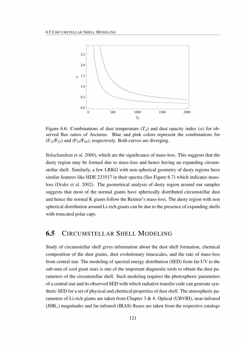
6.5 CIRCUMSTELLAR SHELL MODELING
0 500 1000 1500 20000.0
0.5
1.0
1.5
2.0
2.5
Td
Α
Figure 6.6: Combinations of dust temperature (Td) and dust opacity index (α) for ob-served flux ratios of Arcturus. Blue and pink colors represent the combinations for(F12/F25) and (F25/F60), respectively. Both curves are diverging.
Balachandran et al. 2000), which are the significance of mass-loss. This suggests that thedusty region may be formed due to mass-loss and hence having an expanding circum-stellar shell. Similarly, a few LRKG with non-spherical geometry of dusty regions havesimilar features like HDE 233517 in their spectra (See Figure 6.7) which indicates mass-loss (Drake et al. 2002). The geometrical analysis of dusty region around our samplessuggests that most of the normal giants have spherically distributed circumstellar dustand hence the normal K giants follow the Reimer’s mass-loss. The dusty region with nonspherical distribution around Li-rich giants can be due to the presence of expanding shellswith truncated polar caps.
6.5 CIRCUMSTELLAR SHELL MODELING
Study of circumstellar shell gives information about the dust shell formation, chemicalcomposition of the dust grains, dust evolutionary timescales, and the rate of mass-lossfrom central star. The modeling of spectral energy distribution (SED) from far-UV to thesub-mm of cool giant stars is one of the important diagnostic tools to obtain the dust pa-rameters of the circumstellar shell. Such modeling requires the photospheric parametersof a central star and its observed SED with which radiative transfer code can generate syn-thetic SED for a set of physical and chemical properties of dust shell. The atmospheric pa-rameters of Li-rich giants are taken from Chapter 3 & 4. Optical (UBVRI), near-infrared(JHKs) magnitudes and far-infrared (IRAS) fluxes are taken from the respective catalogs
121
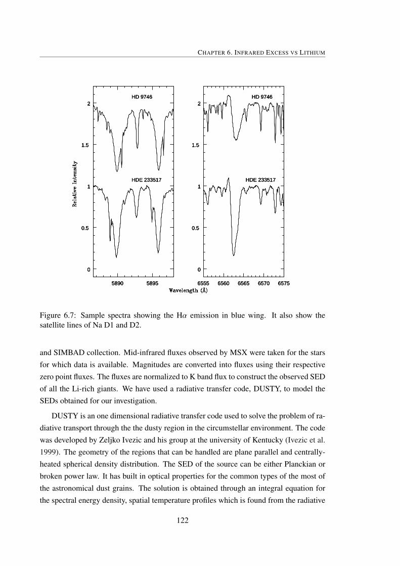
CHAPTER 6. INFRARED EXCESS VS LITHIUM
5890 5895
0
0.5
1
1.5
2
HDE 233517
HD 9746
6555 6560 6565 6570 6575
0
0.5
1
1.5
2
HDE 233517
HD 9746
5890 5895
0
0.5
1
1.5
2
HDE 233517
HD 9746
6555 6560 6565 6570 6575
0
0.5
1
1.5
2
HDE 233517
HD 9746
5890 5895
0
0.5
1
1.5
2
HDE 233517
HD 9746
6555 6560 6565 6570 6575
0
0.5
1
1.5
2
HDE 233517
HD 9746
Figure 6.7: Sample spectra showing the Hα emission in blue wing. It also show thesatellite lines of Na D1 and D2.
and SIMBAD collection. Mid-infrared fluxes observed by MSX were taken for the starsfor which data is available. Magnitudes are converted into fluxes using their respectivezero point fluxes. The fluxes are normalized to K band flux to construct the observed SEDof all the Li-rich giants. We have used a radiative transfer code, DUSTY, to model theSEDs obtained for our investigation.
DUSTY is an one dimensional radiative transfer code used to solve the problem of ra-diative transport through the the dusty region in the circumstellar environment. The codewas developed by Zeljko Ivezic and his group at the university of Kentucky (Ivezic et al.1999). The geometry of the regions that can be handled are plane parallel and centrally-heated spherical density distribution. The SED of the source can be either Planckian orbroken power law. It has built in optical properties for the common types of the most ofthe astronomical dust grains. The solution is obtained through an integral equation forthe spectral energy density, spatial temperature profiles which is found from the radiative
122
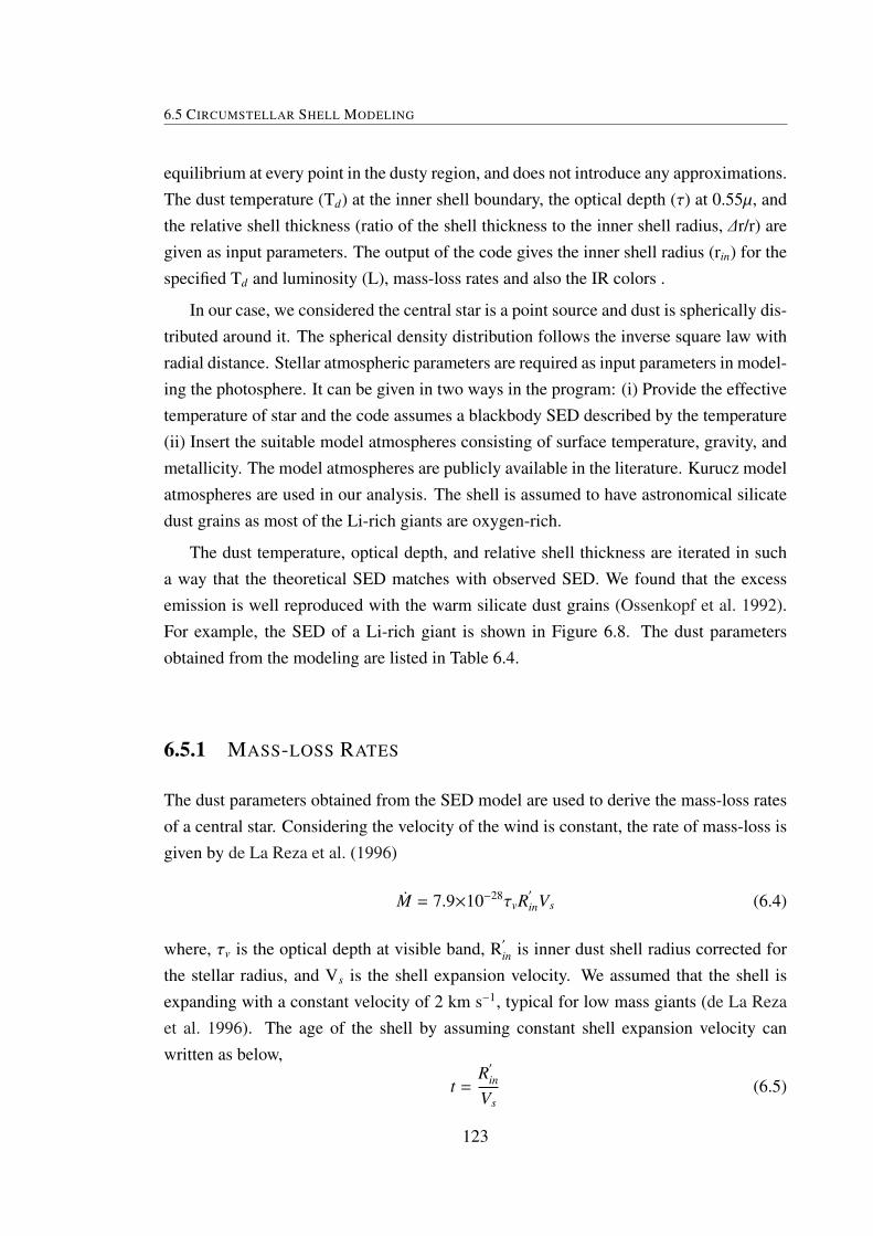
6.5 CIRCUMSTELLAR SHELL MODELING
equilibrium at every point in the dusty region, and does not introduce any approximations.The dust temperature (Td) at the inner shell boundary, the optical depth (τ) at 0.55µ, andthe relative shell thickness (ratio of the shell thickness to the inner shell radius, ∆r/r) aregiven as input parameters. The output of the code gives the inner shell radius (rin) for thespecified Td and luminosity (L), mass-loss rates and also the IR colors .
In our case, we considered the central star is a point source and dust is spherically dis-tributed around it. The spherical density distribution follows the inverse square law withradial distance. Stellar atmospheric parameters are required as input parameters in model-ing the photosphere. It can be given in two ways in the program: (i) Provide the effectivetemperature of star and the code assumes a blackbody SED described by the temperature(ii) Insert the suitable model atmospheres consisting of surface temperature, gravity, andmetallicity. The model atmospheres are publicly available in the literature. Kurucz modelatmospheres are used in our analysis. The shell is assumed to have astronomical silicatedust grains as most of the Li-rich giants are oxygen-rich.
The dust temperature, optical depth, and relative shell thickness are iterated in sucha way that the theoretical SED matches with observed SED. We found that the excessemission is well reproduced with the warm silicate dust grains (Ossenkopf et al. 1992).For example, the SED of a Li-rich giant is shown in Figure 6.8. The dust parametersobtained from the modeling are listed in Table 6.4.
6.5.1 MASS-LOSS RATES
The dust parameters obtained from the SED model are used to derive the mass-loss ratesof a central star. Considering the velocity of the wind is constant, the rate of mass-loss isgiven by de La Reza et al. (1996)
M = 7.9×10⁻²⁸τvR′
inVs (6.4)
where, τv is the optical depth at visible band, R′
in is inner dust shell radius corrected forthe stellar radius, and Vs is the shell expansion velocity. We assumed that the shell isexpanding with a constant velocity of 2 km s−1, typical for low mass giants (de La Rezaet al. 1996). The age of the shell by assuming constant shell expansion velocity canwritten as below,
t =R′
in
Vs(6.5)
123

CHAPTER 6. INFRARED EXCESS VS LITHIUM
0 0.5 1 1.5
-13
-12
-11
-10
0 0.5 1 1.5
-13
-12
-11
-10
0 0.5 1 1.5
-13
-12
-11
-10
0 0.5 1 1.5
-13
-12
-11
-10
Figure 6.8: Spectral energy distribution of observed fluxes superposed with the theoreticalfluxes modeled from DUSTY.
where t is the time taken to shell expanding to R′
in. The age of the shell and mass-lossrates of Li-rich giants are derived and are given in Table 6.4. In the table, most of thegiants are having mass-loss rates in the range of 10−10 to 10−8 M yr−1. The age of theshells are in the range of 103 to 105 years.
Luminosity driven mass-loss rates for normal giants in all the 4 bins (viz pre-bump,bump, clumps, post bump) are derived using the modified version of the Reimer’s law(Schroder & Cuntz 2005)
M =ηL?R?
M?
(Te f f
4000)(1 +
g4300g?
) (6.6)
Where η = 8±1×10⁻¹⁴ M yr−1. L?, R?, M?, g? are Luminosity, Radius, Mass, andsurface gravity of star, respectively. Te f f is the surface temperature of the star and wetook a value of solar gravity, log g = 4.44. Radius for the stars are calculated fromtheir luminosities and temperatures. Parallax based gravities are obtained using the aboveparameters and the following equation:
logg = logLL
+ logMM
+ 4logTe f f − 10.61 (6.7)
124
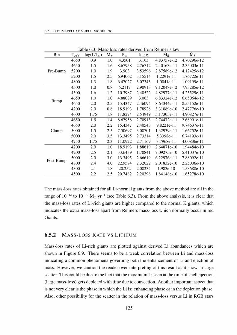
6.5 CIRCUMSTELLAR SHELL MODELING
Table 6.3: Mass-loss rates derived from Reimer’s lawBin Te f f log(L/L) M? R? log g MR MS
Pre-Bump
4650 0.9 1.0 4.3501 3.163 4.83757e-12 4.70296e-124650 1.5 1.6 8.67958 2.76712 2.40163e-11 2.35003e-115200 1.0 1.9 3.903 3.53596 2.87589e-12 4.12425e-125200 1.5 2.5 6.94062 3.15514 1.2291e-11 1.76722e-114800 1.3 1.8 6.47027 3.07343 1.0041e-11 1.09199e-11
Bump
4500 1.0 0.8 5.2117 2.90913 9.12048e-12 7.93285e-124500 1.6 1.2 10.3987 2.48522 4.82977e-11 4.25529e-114650 1.0 1.0 4.88089 3.063 6.83324e-12 6.65064e-124650 2.0 2.5 15.4347 2.46094 8.64344e-11 8.55152e-114200 2.0 0.8 18.9193 1.78928 3.31089e-10 2.47776e-104600 1.75 1.8 11.8274 2.54949 5.17303e-11 4.90827e-11
Clump
4650 1.5 1.4 8.67958 2.70913 2.74472e-11 2.68991e-114650 2.0 2.2 15.4347 2.40543 9.8221e-11 9.74637e-115000 1.5 2.5 7.50697 3.08701 1.32939e-11 1.66752e-115000 2.0 3.5 13.3495 2.73314 5.3398e-11 6.74193e-114750 1.75 2.3 11.0922 2.71169 3.7968e-11 4.00836e-11
Post-Bump
4200 2.0 1.0 18.9193 1.88619 2.64871e-10 1.94484e-104200 2.5 2.1 33.6439 1.70841 7.09275e-10 5.41037e-105000 2.0 3.0 13.3495 2.66619 6.22976e-11 7.88092e-114800 2.4 4.0 22.9574 2.32022 2.01832e-10 2.25006e-104300 2.1 1.8 20.252 2.08234 1.983e-10 1.53688e-104500 2.2 2.5 20.7482 2.20398 1.84148e-10 1.65278e-10
The mass-loss rates obtained for all Li-normal giants from the above method are all in therange of 10−12 to 10−10 M yr−1 (see Table 6.3). From the above analysis, it is clear thatthe mass-loss rates of Li-rich giants are higher compared to the normal K giants, whichindicates the extra mass-loss apart from Reimers mass-loss which normally occur in redGiants.
6.5.2 MASS-LOSS RATE VS LITHIUM
Mass-loss rates of Li-rich giants are plotted against derived Li abundances which areshown in Figure 6.9. There seems to be a weak correlation between Li and mass-lossindicating a common phenomena governing both the enhancement of Li and ejection ofmass. However, we caution the reader over-interpreting of this result as it shows a largescatter. This could be due to the fact that the maximum Li seen at the time of shell ejection(large mass-loss) gets depleted with time due to convection. Another important aspect thatis not very clear is the phase in which the Li is: enhancing phase or in the depletion phase.Also, other possibility for the scatter in the relation of mass-loss versus Li in RGB stars
125

CHAPTER 6. INFRARED EXCESS VS LITHIUM
Table 6.4: Photospheric and dust parameters of Li-rich K giants.Star A(Li) Te f f Log(L/L) R/R M Tdust thd40168 1.50 4800 2.14 17.0185 8.20300e-10 55 4120.46hd116292 1.50 4870 1.83 11.5704 7.35389e-11 95 615.656hd40827 1.60 4575 1.79 12.5205 1.29562e-10 110 371.889hd88476 1.60 4950 1.87 11.7272 3.57581e-10 75 1330.5hd63798 1.75 5000 1.78 10.3625 5.12552e-09 28 20596.8hd787 1.80 4180 2.71 43.2566 2.48527e-11 180 249.675hd12203 1.80 4850 1.69 9.92936 4.23622e-10 65 1576.22hd133086 1.80 4850 1.70 10.0443 3.54807e-09 30 16202.1hd90633 1.85 4800 1.56 8.72815 4.39417e-11 100 367.873hd120602 1.90 5000 1.98 13.0456 2.77807e-10 70 1860.6hd183492 2.00 4700 1.74 11.1998 7.02149e-10 110 352.697hd148293 2.00 4640 1.87 13.3465 4.75923e-13 250 47.8122hd107484 2.00 4500 1.78 12.7932 2.19865e-09 63 1840.68hd118319 2.00 4750 1.69 10.3518 6.25045e-10 40 6279.33hd146850 2.00 4200 2.90 53.322 4.50029e-09 60 6458.69hd108471 2.00 4970 1.85 11.3682 8.82667e-10 65 2955.82hd203136 2.23 4980 1.76 10.2081 3.83363e-09 80 962.838I17596 2.30 4600 1.70 11.1658 2.37905e-08 190 85.3588hd145457 2.40 4880 1.61 8.94469 4.64719e-11 80 466.867hd51367 2.50 4700 1.59 9.42343 3.43837e-10 60 1727.13pds100 2.50 4500 1.70 11.6676 1.48663e-08 250 29.87hd217352 2.64 4600 1.78 12.243 1.03377e-10 105 399.44hd112127 2.70 4340 1.42 9.0871 9.77463e-11 60 1309.31hd150902 2.70 4700 1.83 12.4225 6.67202e-10 90 670.286hd37719 2.80 4700 1.76 11.4606 2.62341e-07 20 52710.6hd39853 2.80 3900 2.66 46.9111 9.44113e-11 110 948.476hd167304 2.85 4860 1.93 13.0356 3.31485e-08 20 66603.3hd6665 2.92 4500 1.43 8.55027 4.39517e-10 95 339.653hd219025 3.00 4570 1.88 13.9179 6.02185e-09 275 40.3312hd170527 3.28 4810 1.69 10.0952 1.60569e-10 65 1613.11hd214995 3.28 4737 1.56 8.96186 4.21595e-08 20 42354.3I13313 3.30 4540 1.85 13.6236 1.29749e-07 260 46.553hd10437 3.49 4830 1.77 10.9777 1.12186e-08 27 22541hd8676 3.58 4860 1.68 9.77535 3.45143e-10 100 433.422hd19745 3.70 4700 1.90 13.4651 3.50690e-09 170 117.437hd9746 3.75 4400 2.04 18.0509 3.42073e-08 22 49093.3hd77361 3.80 4580 1.66 10.7566 7.70440e-09 30 12900I13539 4.05 4300 1.60 11.3885 3.27951e-08 230 47.0666hd233517 4.22 4475 2.00 16.6655 1.88577e-07 75 1262.99
126
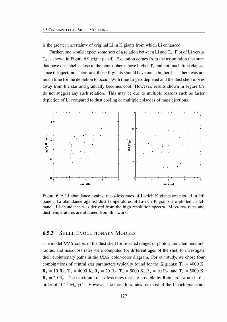
6.5 CIRCUMSTELLAR SHELL MODELING
is the greater uncertainty of original Li in K giants from which Li enhanced.
Further, one would expect some sort of a relation between Li and Td. Plot of Li versusTd is shown in Figure 6.9 (right panel). Exception comes from the assumption that starsthat have dust shells close to the photospheres have higher Td and not much time elapsedsince the ejection. Therefore, those K giants should have much higher Li as there was notmuch time for the depletion to occur. With time Li gets depleted and the dust shell movesaway from the star and gradually becomes cool. However, results shown in Figure 6.9do not suggest any such relation. This may be due to multiple reasons such as fasterdepletion of Li compared to dust cooling or multiple episodes of mass ejections.
1 2 3 4 5-12
-10
-8
-6
1 2 3 4 5-12
-10
-8
-6
1 2 3 4 5-12
-10
-8
-6
1 2 3 4 5-12
-10
-8
-6
1 2 3 4 51
1.5
2
2.5
3
1 2 3 4 51
1.5
2
2.5
3
1 2 3 4 51
1.5
2
2.5
3
Figure 6.9: Li abundance against mass-loss rates of Li-rich K giants are plotted in leftpanel. Li abundance against dust temperatures of Li-rich K giants are plotted in leftpanel. Li abundance was derived from the high resolution spectra. Mass-loss rates anddust temperatures are obtained from this work.
6.5.3 SHELL EVOLUTIONARY MODELS
The model IRAS colors of the dust shell for selected ranges of photospheric temperature,radius, and mass-loss rates were computed for different ages of the shell to investigatetheir evolutionary paths in the IRAS color-color diagram. For our study, we chose fourcombinations of central star parameters typically found for the K giants: T? = 4000 K,R? = 10 R, T? = 4000 K, R? = 20 R, T? = 5000 K, R? = 10 R, and T? = 5000 K,R? = 20 R. The maximum mass-loss rates that are possible by Reimers law are in theorder of 10−10 M yr−1. However, the mass-loss rates for most of the Li-rich giants are
127

CHAPTER 6. INFRARED EXCESS VS LITHIUM
in between 10−10 and 10−8 M yr−1. We have made our computations for a set of fourmass-loss rates of 10−10, 10−9, 5×10⁻⁹, and 3×10⁻⁸ M yr−1. Further, we assume that thestar has encountered mass-loss for a duration of around 1000 yrs to calculate the physicalthickness of the shell (as we found from the models of SED of known LRKG). The relativethickness of the shell varies from 35 to 0.017. The hottest dust considered is at 1500 K (atAge = 0) which is the sublimation temperature for silicates, and the coolest dust around10 K which is almost near the ISM dust temperature. At first, we have estimated thephotospheric colors by assuming no dust around it. In all our models, we considered thecolors at dust formation temperature as the starting point and stellar photospheric coloras the ending points of the evolutionary loop. This point represents cases where the shellmight not have formed yet or it is expanded and fully dissipated into interstellar medium.Intense mass-loss creates a thick shell with peak dust temperature of 1500 K, with time,as the shell expands it becomes thinner and cooler and finally the shell will dissipate intothe interstellar medium.
Table 6.5: Dust parameters and evolutionary timescales for different photospheric param-eters
M T? R? Td AgeMyr−1 °K R °K yr
1×10−104000
10 25 1654820 28 23641
500010 27 3780220 31 50164
1×10−94000
10 17 5216320 19 74736
500010 19 10767520 20.5 171636
5×10−94000
10 15 7595720 16 125070
500010 15.5 19886820 17 300273
3×10−84000
10 13 11668120 13.5 208958
500010 13.5 29919820 14 537481
The evolutionary paths of the dust shell in the IRAS color-color diagram are shown inFigure 6.10. In the models, the colors are less effected due to the change in temperaturebut significant changes in colors are observed due to increasing radius. The dust parame-
128

6.6 DISCUSSION AND CONCLUSIONS
ters including the evolutionary timescales for all the models are given in Table 6.5 & ??,where Tdust is the dust temperature and age represents the duration of dust shell evolution.The looping timescales for all the models are in between 1.65×10⁴ and 5.37×10⁵ yrs. Theevolutionary timescales are increased more than 50% with increasing radius of 20R and25% increased with increasing temperature of 1000 K.
6.6 DISCUSSION AND CONCLUSIONS
FIR colors of Li-rich giants with all available data are presented on dust evolutionarymodels and is shown in Figure 6.10. All the giants taken for the study are fitted wellinside the modeled loops, except one star HDE 233517, whose mass-loss rate is of theorder of 10−7 M yr−1. Red square is Arcturus, a typical K giant, which is inside thesmallest loop which corresponds to very little mass-loss of the order of 1×10⁻¹⁰ M yr−1.The Li-rich giants occupy regions at the hotter side of the loops indicating these have
-1 -0.5 0 0.5
-1.5
-1
-0.5
0
0.5
-1 -0.5 0 0.5
-1.5
-1
-0.5
0
0.5
-1 -0.5 0 0.5
-1.5
-1
-0.5
0
0.5
-1 -0.5 0 0.5
-1.5
-1
-0.5
0
0.5
-1 -0.5 0 0.5
-1.5
-1
-0.5
0
0.5
-1 -0.5 0 0.5
-1.5
-1
-0.5
0
0.5
-1 -0.5 0 0.5
-1.5
-1
-0.5
0
0.5
-1 -0.5 0 0.5
-1.5
-1
-0.5
0
0.5
Figure 6.10: Sample giants and dust shell evolutionary models are on color-color diagram.Li-rich giants with various quality data are presented on left panel. On the right panel,Li-rich and normal giants with only good quality of data are presented. Different colors,magenta, green, cyan and blue represents the loops of the evolution of a dust shell withmass-loss rates, 1×10⁻¹⁰, 1×10⁻⁹, 5×10⁻⁹, and 3×10⁻⁸, respectively. Four varieties oflines in each color indicate the different photospheric temperatures and radius, Te f f =5000 K, R = 20 R, Te f f = 4000 K, R = 20 R, Te f f = 5000 K, R = 10 R, Te f f = 4000 K,R = 10 R of the dust shell hosting stars, radially outwards, respectively.
129
CHAPTER 6. INFRARED EXCESS VS LITHIUM
relatively warmer shells and the mass-loss episode occured recently. The mass-loss ratescorrespond to the loops are in between 1×10⁻⁹ and 3×10⁻⁸ M yr−1. The dust tempera-tures are in between 100 to 80 K and the respective timescales are 300 to 550 yrs. Li-richand normal giants with only good quality data are shown in Figure 6.10 (right panel).Most of the normal giants in the Figure 6.10 are occupying the smallest loop (magenta),corresponding to little or no mass-loss or the mass-loss rate is comparable to Remer’smass-loss which is about 1×10⁻¹⁰ M yr−1. Interestingly, all the Li-rich K giants are inthe loops of higher mass-loss rates. As shown in Figure 6.10, they have mass-loss rates ofabout 1×10⁻⁹ M yr−1 to 3×10⁻⁸ M yr−1 and have dust temperatures ranging from from80 to 100 K. Also, there a few Li-normal giants that do lie in the high mass-loss loopsbut the giants show cooler Td in the range of 30 K to 60 K. As shown in the Figure 6.10,the super-Li rich K giants have Td around 100 K. The giants with peak Li values have thedust temperature around 100 K but they are in different loops meaning they have range ofmass-loss. The scatter in the earlier plot of Td versus Li (Figure 6.9) perhaps due to thissituation. The corresponding timescale for dust evolution for K giants with Td ∼ 100 Kis about 1000 years and they have mass-loss rates ranging from 10−9 M yr−1 to 10−8 M
yr−1. Considering that the mass-loss begins at the center of inner most loop (small loop),depending on mass and radius, their dust shells evolve along the loops with correspond-ing mass-loss rates and finally join the same inner most loop after losing most of the dustshell into space. Evolutionary periods correspond to a range of periods starting for a fewthousand years in the case of stars of least mass-loss rates to five hundred thousand yearsfor giants of high mass-loss rates (see Table 6.5). Given the good data for a very smallfraction of stars and the other uncertainties described above it is not very straightforwardto suggest a one-to-one correlation with Li evolution with that of dust evolution.
However, by combining the IR CCDm and the HR diagram, we could infer somegross relations between Li and the dust evolution. As shown in FIR CCDm (Figure 6.3),the Li-rich K giants that are occupying bump position in the HR diagram show excessflux at 25µ and 60µ. The Li-rich giants that occupy clump region whose excess flux onlyat 60µ. This is an interesting result. Based on the dust cooling one may argue that themass-loss was perhaps began during its bump evolution. The star evolved and passedthrough RGB tip and settled at the clump region where one naturally expects some coolerdust. If the Li enhancement too began during the bump evolution and one would expecta very little Li by the time it settles at the clump. However, we do have super Li-richgiants both at the clump and at the bump though the clump and bump giants, in this case,could not be separated for sure. Assuming that all the Li-rich giants are located at the
130

6.6 DISCUSSION AND CONCLUSIONS
bump and the non detection of Li-rich K giants above the bump, one would argue thatthe Li evolutionary period is quite small or comparable to the bump evolutionary periods(see Table 6.6). Our modeling of dust shells suggest the periods are of the order of a fewthousand to hundred thousand years. The model results are given in Table 6.5.
Table 6.6: Evolutionary timescales from bump to clumpM/M tbump tbumpbegin−tip tbumpend−tip tclump
1.0 1.525000e+07 1.278400e+08 1.125900e+08 9.492500e+071.2 1.117600e+07 9.879300e+07 8.761700e+07 7.988305e+071.4 8.128000e+06 7.503300e+07 6.690500e+07 7.613281e+071.6 6.856000e+06 5.685500e+07 4.999900e+07 8.077742e+071.8 4.070000e+06 3.547000e+07 3.140000e+07 9.170689e+072.0 2.450000e+06 1.955300e+07 1.710300e+07 1.032371e+08
The timescales of important stages along the RGB are derived from evolutionarytracks (Bertelli 2008) which are given in Table 6.6. In Table 6.6, tbump is the durationof time star spends at the luminosity bump, tbumpbegin−tip is the time taken from the be-ginning of bump to the RGB tip, tbumpend−tip is the time duration that star takes to reachthe RGB tip from the end of bump, and tclump is the time duration that star spends at thered clump. The results suggest an upper limit for Li evolution which is the tbump. This ismuch smaller value compared to the dust evolution which is of the order of a few hundredthousand years.
Now the issue is the whether it is same dust that originated at the bump that is coolingoff at the red clump? The timescales that require for a star to go from bump to the clumpare of the order of 108 years. Since the dust evolutionary time scales are much smallercompared to star’s evolution, one would not expect any IR excess on the giants at theclump. The IR excess perhaps could be the result of core He-flash at the RGB tip andone can suspect that even Li could have been synthesized at that time. Since evolutionarytimescales from the tip to the clump are small one would expect very large amounts of Liat clump giants. Also, since the clump timescales are of the order of a few million years,one would expect to see giants with a range of IR excess from very little to strong excess.The fact that there are a very few Li-rich giants even at the clump, we suggest that Lienhanced during the core He-flash is getting depleted rapidly.
131
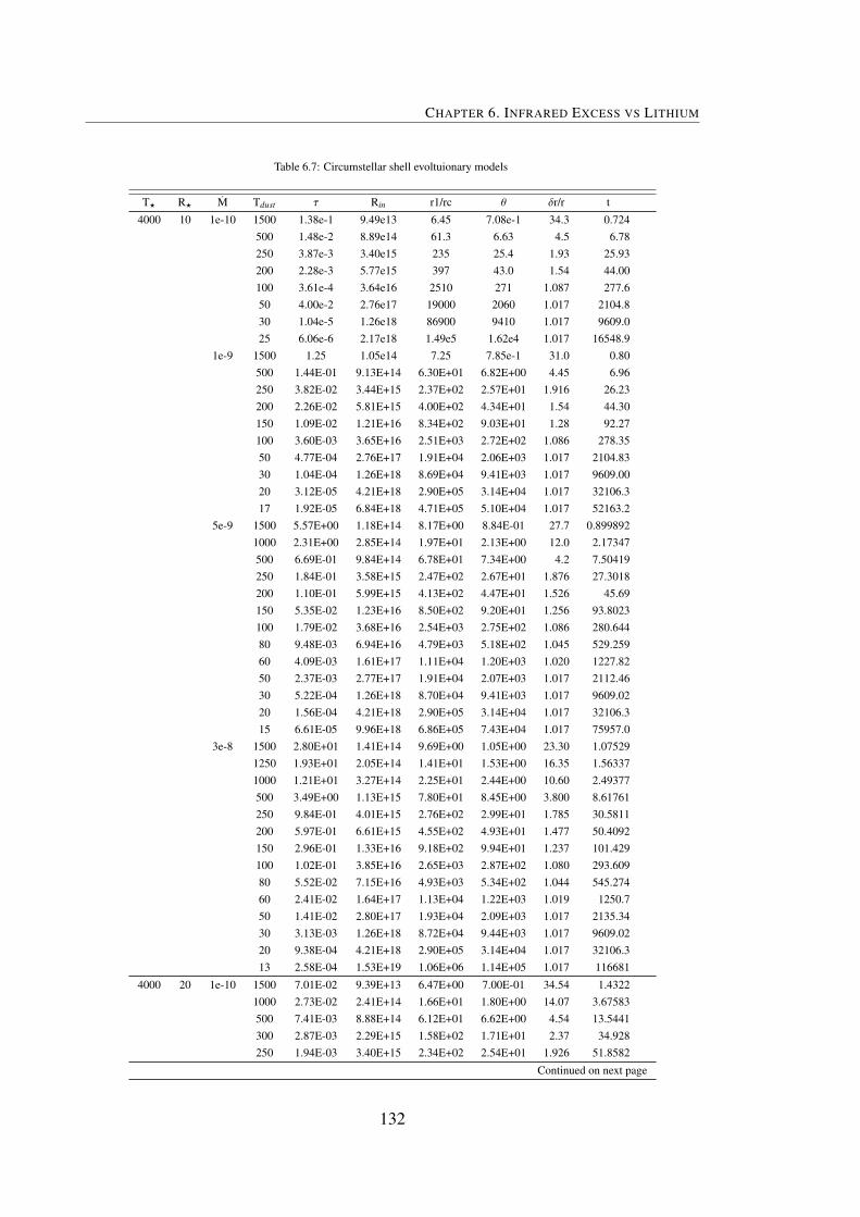
CHAPTER 6. INFRARED EXCESS VS LITHIUM
Table 6.7: Circumstellar shell evoltuionary models
T? R? M Tdust τ Rin r1/rc θ δr/r t
4000 10 1e-10 1500 1.38e-1 9.49e13 6.45 7.08e-1 34.3 0.724500 1.48e-2 8.89e14 61.3 6.63 4.5 6.78250 3.87e-3 3.40e15 235 25.4 1.93 25.93200 2.28e-3 5.77e15 397 43.0 1.54 44.00100 3.61e-4 3.64e16 2510 271 1.087 277.650 4.00e-2 2.76e17 19000 2060 1.017 2104.830 1.04e-5 1.26e18 86900 9410 1.017 9609.025 6.06e-6 2.17e18 1.49e5 1.62e4 1.017 16548.9
1e-9 1500 1.25 1.05e14 7.25 7.85e-1 31.0 0.80500 1.44E-01 9.13E+14 6.30E+01 6.82E+00 4.45 6.96250 3.82E-02 3.44E+15 2.37E+02 2.57E+01 1.916 26.23200 2.26E-02 5.81E+15 4.00E+02 4.34E+01 1.54 44.30150 1.09E-02 1.21E+16 8.34E+02 9.03E+01 1.28 92.27100 3.60E-03 3.65E+16 2.51E+03 2.72E+02 1.086 278.3550 4.77E-04 2.76E+17 1.91E+04 2.06E+03 1.017 2104.8330 1.04E-04 1.26E+18 8.69E+04 9.41E+03 1.017 9609.0020 3.12E-05 4.21E+18 2.90E+05 3.14E+04 1.017 32106.317 1.92E-05 6.84E+18 4.71E+05 5.10E+04 1.017 52163.2
5e-9 1500 5.57E+00 1.18E+14 8.17E+00 8.84E-01 27.7 0.8998921000 2.31E+00 2.85E+14 1.97E+01 2.13E+00 12.0 2.17347500 6.69E-01 9.84E+14 6.78E+01 7.34E+00 4.2 7.50419250 1.84E-01 3.58E+15 2.47E+02 2.67E+01 1.876 27.3018200 1.10E-01 5.99E+15 4.13E+02 4.47E+01 1.526 45.69150 5.35E-02 1.23E+16 8.50E+02 9.20E+01 1.256 93.8023100 1.79E-02 3.68E+16 2.54E+03 2.75E+02 1.086 280.64480 9.48E-03 6.94E+16 4.79E+03 5.18E+02 1.045 529.25960 4.09E-03 1.61E+17 1.11E+04 1.20E+03 1.020 1227.8250 2.37E-03 2.77E+17 1.91E+04 2.07E+03 1.017 2112.4630 5.22E-04 1.26E+18 8.70E+04 9.41E+03 1.017 9609.0220 1.56E-04 4.21E+18 2.90E+05 3.14E+04 1.017 32106.315 6.61E-05 9.96E+18 6.86E+05 7.43E+04 1.017 75957.0
3e-8 1500 2.80E+01 1.41E+14 9.69E+00 1.05E+00 23.30 1.075291250 1.93E+01 2.05E+14 1.41E+01 1.53E+00 16.35 1.563371000 1.21E+01 3.27E+14 2.25E+01 2.44E+00 10.60 2.49377500 3.49E+00 1.13E+15 7.80E+01 8.45E+00 3.800 8.61761250 9.84E-01 4.01E+15 2.76E+02 2.99E+01 1.785 30.5811200 5.97E-01 6.61E+15 4.55E+02 4.93E+01 1.477 50.4092150 2.96E-01 1.33E+16 9.18E+02 9.94E+01 1.237 101.429100 1.02E-01 3.85E+16 2.65E+03 2.87E+02 1.080 293.60980 5.52E-02 7.15E+16 4.93E+03 5.34E+02 1.044 545.27460 2.41E-02 1.64E+17 1.13E+04 1.22E+03 1.019 1250.750 1.41E-02 2.80E+17 1.93E+04 2.09E+03 1.017 2135.3430 3.13E-03 1.26E+18 8.72E+04 9.44E+03 1.017 9609.0220 9.38E-04 4.21E+18 2.90E+05 3.14E+04 1.017 32106.313 2.58E-04 1.53E+19 1.06E+06 1.14E+05 1.017 116681
4000 20 1e-10 1500 7.01E-02 9.39E+13 6.47E+00 7.00E-01 34.54 1.43221000 2.73E-02 2.41E+14 1.66E+01 1.80E+00 14.07 3.67583500 7.41E-03 8.88E+14 6.12E+01 6.62E+00 4.54 13.5441300 2.87E-03 2.29E+15 1.58E+02 1.71E+01 2.37 34.928250 1.94E-03 3.40E+15 2.34E+02 2.54E+01 1.926 51.8582
Continued on next page
132
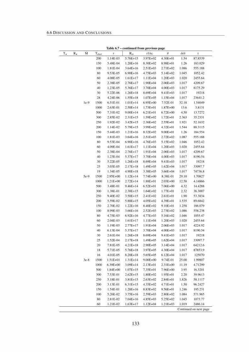
6.6 DISCUSSION AND CONCLUSIONS
Table 6.7 – continued from previous pageT? R? M Tdust τ Rin r1/rc θ δr/r t
200 1.14E-03 5.76E+15 3.97E+02 4.30E+01 1.54 87.8539150 5.48E-04 1.20E+16 8.30E+02 8.98E+01 1.26 183.029100 1.81E-04 3.64E+16 2.51E+03 2.71E+02 1.086 555.18880 9.53E-05 6.90E+16 4.75E+03 5.14E+02 1.045 1052.4260 4.08E-05 1.61E+17 1.11E+04 1.20E+03 1.020 2455.6450 2.38E-05 2.76E+17 1.90E+04 2.06E+03 1.017 4209.6740 1.23E-05 5.36E+17 3.70E+04 4.00E+03 1.017 8175.2930 5.22E-06 1.26E+18 8.69E+04 9.41E+03 1.017 1921828 4.24E-06 1.55E+18 1.07E+05 1.15E+04 1.017 23641.2
1e-9 1500 6.51E-01 1.01E+14 6.95E+00 7.52E-01 32.18 1.540491000 2.63E-01 2.50E+14 1.73E+01 1.87E+00 13.6 3.8131500 7.31E-02 9.00E+14 6.21E+01 6.72E+00 4.50 13.7272300 2.85E-02 2.31E+15 1.59E+02 1.72E+01 2.363 35.2331250 1.92E-02 3.42E+15 2.36E+02 2.55E+01 1.921 52.1632200 1.14E-02 5.79E+15 3.99E+02 4.32E+01 1.544 88.3115150 5.44E-03 1.21E+16 8.32E+02 9.00E+01 1.26 184.554100 1.81E-03 3.64E+16 2.51E+03 2.72E+02 1.087 555.18880 9.53E-04 6.90E+16 4.76E+03 5.15E+02 1.046 1052.4260 4.09E-04 1.61E+17 1.11E+04 1.20E+03 1.020 2455.6450 2.38E-04 2.76E+17 1.91E+04 2.06E+03 1.017 4209.6740 1.23E-04 5.37E+17 3.70E+04 4.00E+03 1.017 8190.5430 5.22E-05 1.26E+18 8.69E+04 9.41E+03 1.017 1921825 3.03E-05 2.17E+18 1.49E+05 1.62E+04 1.017 33097.719 1.34E-05 4.90E+18 3.38E+05 3.66E+04 1.017 74736.8
5e-9 1500 2.95E+00 1.12E+14 7.74E+00 8.38E-01 29.10 1.708271000 1.21E+00 2.72E+14 1.88E+01 2.03E+00 12.58 4.14866500 3.48E-01 9.46E+14 6.52E+01 7.06E+00 4.32 14.4288300 1.38E-01 2.38E+15 1.64E+02 1.77E+01 2.32 36.3007250 9.40E-02 3.50E+15 2.41E+02 2.61E+01 1.90 53.3834200 5.59E-02 5.88E+15 4.05E+02 4.39E+01 1.535 89.6842150 2.70E-02 1.22E+16 8.40E+02 9.10E+01 1.258 186.079100 8.99E-03 3.66E+16 2.52E+03 2.73E+02 1.086 558.23880 4.75E-03 6.92E+16 4.77E+03 5.16E+02 1.046 1055.4760 2.04E-03 1.61E+17 1.11E+04 1.20E+03 1.020 2455.6450 1.19E-03 2.77E+17 1.91E+04 2.06E+03 1.017 4224.9240 6.13E-04 5.37E+17 3.70E+04 4.00E+03 1.017 8190.5430 2.61E-04 1.26E+18 8.69E+04 9.41E+03 1.017 1921825 1.52E-04 2.17E+18 1.49E+05 1.62E+04 1.017 33097.720 7.81E-05 4.21E+18 2.90E+05 3.14E+04 1.017 64212.618 5.71E-05 5.76E+18 3.97E+05 4.30E+04 1.017 87853.916 4.01E-05 8.20E+18 5.65E+05 6.12E+04 1.017 125070
3e-8 1500 1.51E+01 1.31E+14 9.00E+00 9.74E-01 25.00 1.998071000 6.39E+00 3.09E+14 2.13E+01 2.31E+00 11.19 4.71299500 1.84E+00 1.07E+15 7.35E+01 7.96E+00 3.95 16.3201300 7.53E-01 2.62E+15 1.80E+02 1.95E+01 2.20 39.9613250 5.18E-01 3.81E+15 2.63E+02 2.84E+01 1.826 58.1117200 3.13E-01 6.31E+15 4.35E+02 4.71E+01 1.50 96.2427150 1.54E-01 1.28E+16 8.83E+02 9.56E+01 1.246 195.231100 5.26E-02 3.75E+16 2.59E+03 2.80E+02 1.084 571.96580 2.81E-02 7.04E+16 4.85E+03 5.25E+02 1.045 1073.7760 1.21E-02 1.63E+17 1.12E+04 1.21E+03 1.019 2486.14
Continued on next page
133

CHAPTER 6. INFRARED EXCESS VS LITHIUM
Table 6.7 – continued from previous pageT? R? M Tdust τ Rin r1/rc θ δr/r t
50 7.10E-03 2.78E+17 1.92E+04 2.08E+03 1.017 4240.1730 1.57E-03 1.26E+18 8.70E+04 9.42E+03 1.017 1921820 4.69E-04 4.21E+18 2.90E+05 3.14E+04 1.017 64212.618 3.42E-04 5.77E+18 3.97E+05 4.30E+04 1.017 88006.415 1.98E-04 9.96E+18 6.86E+05 7.43E+04 1.017 151914
13.5 1.44E-04 1.37E+19 9.42E+05 1.02E+05 1.017 208958
5000 10 1e-10 1500 4.87E-02 1.15E+14 1.24E+01 8.60E-01 28.4 2.060341000 1.89E-02 2.96E+14 3.19E+01 2.21E+00 11.6 5.30315800 1.19E-02 4.69E+14 5.06E+01 3.50E+00 7.71 8.40262500 5.14E-03 1.09E+15 1.17E+02 8.12E+00 3.88 19.5285300 1.99E-03 2.81E+15 3.02E+02 2.10E+01 2.12 50.3441250 1.34E-03 4.17E+15 4.49E+02 3.11E+01 1.755 74.7099200 7.93E-04 7.06E+15 7.60E+02 5.27E+01 1.446 126.487150 3.81E-04 1.47E+16 1.59E+03 1.10E+02 1.214 263.366100 1.26E-04 4.46E+16 4.80E+03 3.32E+02 1.071 799.05580 6.63E-05 8.45E+16 9.10E+03 6.30E+02 1.037 1513.9060 2.84E-05 1.97E+17 2.12E+04 1.47E+03 1.017 3529.4650 1.66E-05 3.38E+17 3.65E+04 2.53E+03 1.017 6055.6240 8.53E-06 6.57E+17 7.08E+04 4.90E+03 1.017 11770.830 3.64E-06 1.54E+18 1.66E+05 1.15E+04 1.017 27590.727 2.65E-06 2.11E+18 2.27E+05 1.58E+04 1.017 37802.8
1e-9 1500 4.45E-01 1.26E+14 1.36E+01 9.39E-01 25.00 2.257421000 1.81E-01 3.10E+14 3.34E+01 2.31E+00 11.16 5.55397800 1.15E-01 4.85E+14 5.23E+01 3.62E+00 7.50 8.68928500 5.05E-02 1.11E+15 1.19E+02 8.27E+00 3.80 19.8868300 1.97E-02 2.84E+15 3.05E+02 2.12E+01 2.10 50.8815250 1.33E-02 4.20E+15 4.52E+02 3.13E+01 1.75 75.2473200 7.89E-03 7.10E+15 7.64E+02 5.29E+01 1.44 127.204150 3.78E-03 1.48E+16 1.59E+03 1.10E+02 1.21 265.157100 1.26E-03 4.46E+16 4.81E+03 3.33E+02 1.071 799.05580 6.63E-04 8.45E+16 9.10E+03 6.31E+02 1.037 1513.960 2.84E-04 1.97E+17 2.12E+04 1.47E+03 1.017 3529.4650 1.65E-04 3.39E+17 3.65E+04 2.53E+03 1.017 6073.5440 8.53E-05 6.57E+17 7.08E+04 4.90E+03 1.017 11770.830 3.64E-05 1.54E+18 1.66E+05 1.15E+04 1.017 27590.725 2.11E-05 2.65E+18 2.86E+05 1.98E+04 1.017 47477.520 1.09E-05 5.16E+18 5.55E+05 3.85E+04 1.017 92446.719 9.32E-06 6.01E+18 6.47E+05 4.48E+04 1.017 107675
5e-9 1500 1.99E+00 1.41E+14 1.52E+01 1.05E+00 23.30 2.526161250 1.32E+00 2.12E+14 2.28E+01 1.58E+00 15.85 3.79821000 8.19E-01 3.42E+14 3.68E+01 2.55E+00 10.21 6.12728800 5.29E-01 5.29E+14 5.70E+01 3.95E+00 6.95 9.47758500 2.37E-01 1.18E+15 1.27E+02 8.78E+00 3.66 21.1409300 9.53E-02 2.94E+15 3.17E+02 2.20E+01 2.070 52.6731250 6.48E-02 4.32E+15 4.66E+02 3.23E+01 1.729 77.3973200 3.86E-02 7.25E+15 7.81E+02 5.41E+01 1.434 129.891150 1.87E-02 1.50E+16 1.62E+03 1.12E+02 1.210 268.74100 6.24E-03 4.49E+16 4.84E+03 3.35E+02 1.070 804.4380 3.30E-03 8.49E+16 9.14E+03 6.33E+02 1.037 1521.0760 1.42E-03 1.97E+17 2.13E+04 1.47E+03 1.017 3529.4650 8.26E-04 3.39E+17 3.65E+04 2.53E+03 1.017 6073.54
Continued on next page
134

6.6 DISCUSSION AND CONCLUSIONS
Table 6.7 – continued from previous pageT? R? M Tdust τ Rin r1/rc θ δr/r t
40 4.26E-04 6.58E+17 7.08E+04 4.91E+03 1.017 11788.730 1.82E-04 1.54E+18 1.66E+05 1.15E+04 1.017 27590.725 1.06E-04 2.65E+18 2.86E+05 1.98E+04 1.017 47477.518 3.97E-05 7.06E+18 7.60E+05 5.27E+04 1.017 126487
15.5 2.52E-05 1.11E+19 1.19E+06 8.25E+04 1.017 1988683e-8 1500 6.46E+00 2.60E+14 2.81E+01 1.94E+00 13.10 4.65817
1000 4.35E+00 3.86E+14 4.16E+01 2.88E+00 9.160 6.91559800 2.80E+00 6.01E+14 6.47E+01 4.49E+00 6.250 10.7675500 1.25E+00 1.34E+15 1.44E+02 1.00E+01 3.350 24.0075400 8.62E-01 1.95E+15 2.10E+02 1.45E+01 2.600 34.9363300 5.09E-01 3.30E+15 3.55E+02 2.46E+01 1.954250 3.50E-01 4.80E+15 5.17E+02 3.58E+01 1.656 85.9970200 2.12E-01 7.93E+15 8.54E+02 5.92E+01 1.397 142.074150 1.05E-01 1.60E+16 1.72E+03 1.19E+02 1.195 286.657100 3.61E-02 4.65E+16 5.00E+03 3.47E+02 1.068 833.09680 1.94E-02 8.68E+16 9.35E+03 6.47E+02 1.036 1555.1160 8.40E-03 2.00E+17 2.15E+04 1.49E+03 1.017 3583.2150 4.93E-03 3.41E+17 3.68E+04 2.55E+03 1.017 6109.3740 2.55E-03 6.60E+17 7.11E+04 4.92E+03 1.017 11824.630 1.08E-03 1.55E+18 1.67E+05 1.15E+04 1.017 27769.925 6.32E-04 2.66E+18 2.86E+05 1.98E+04 1.017 47656.618 2.38E-04 7.06E+18 7.61E+05 5.27E+04 1.017 12648714 1.12E-04 1.50E+19 1.62E+06 1.12E+05 1.017 268740
13.5 1.01E-04 1.67E+19 1.80E+06 1.25E+05 1.017 299198
5000 20 1e-10 1500 2.46E-02 1.14E+14 1.23E+01 8.54E-01 28.6 4.084861250 1.58E-02 1.77E+14 1.91E+01 1.32E+00 18.7 6.342281000 9.49E-03 2.95E+14 3.18E+01 2.20E+00 11.06 10.5705800 5.97E-03 4.69E+14 5.05E+01 3.50E+00 7.700 16.8052500 2.57E-03 1.09E+15 1.17E+02 8.11E+00 3.88 39.057300 9.97E-04 2.81E+15 3.02E+02 2.09E+01 2.12 100.688250 6.73E-04 4.16E+15 4.48E+02 3.11E+01 1.756 149.061200 3.97E-04 7.06E+15 7.60E+02 5.27E+01 1.446 252.974150 1.91E-04 1.47E+16 1.59E+03 1.10E+02 1.214100 6.28E-05 4.46E+16 4.80E+03 3.32E+02 1.07080 3.32E-05 8.44E+16 9.09E+03 6.30E+02 1.03760 1.42E-05 1.97E+17 2.12E+04 1.47E+03 1.01750 8.29E-06 3.38E+17 3.65E+04 2.53E+03 1.017 12111.240 4.26E-06 6.57E+17 7.08E+04 4.90E+03 1.017 23541.735 2.87E-06 9.77E+17 1.05E+05 7.29E+03 1.017 35007.931 2.00E-06 1.40E+18 1.51E+05 1.05E+04 1.017 50164.9
1e-9 1500 2.31E-01 1.21E+14 1.30E+01 9.02E-01 27.00 4.335681250 1.52E-01 1.84E+14 1.98E+01 1.37E+00 18.10 6.59311000 9.24E-02 3.03E+14 3.26E+01 2.26E+00 11.39 10.8571800 5.87E-02 4.77E+14 5.14E+01 3.56E+00 7.60 17.0919500 2.55E-02 1.10E+15 1.18E+02 8.18E+00 3.86 39.4153300 9.93E-03 2.82E+15 3.04E+02 2.10E+01 2.11 101.046250 6.70E-03 4.18E+15 4.50E+02 3.12E+01 1.75 149.778200 3.96E-03 7.08E+15 7.62E+02 5.28E+01 1.44 253.691150 1.89E-03 1.48E+16 1.59E+03 1.10E+02 1.21 530.315100 6.28E-04 4.46E+16 4.80E+03 3.33E+02 1.07 1598.1180 3.31E-04 8.45E+16 9.10E+03 6.30E+02 1.037 3027.81
Continued on next page
135
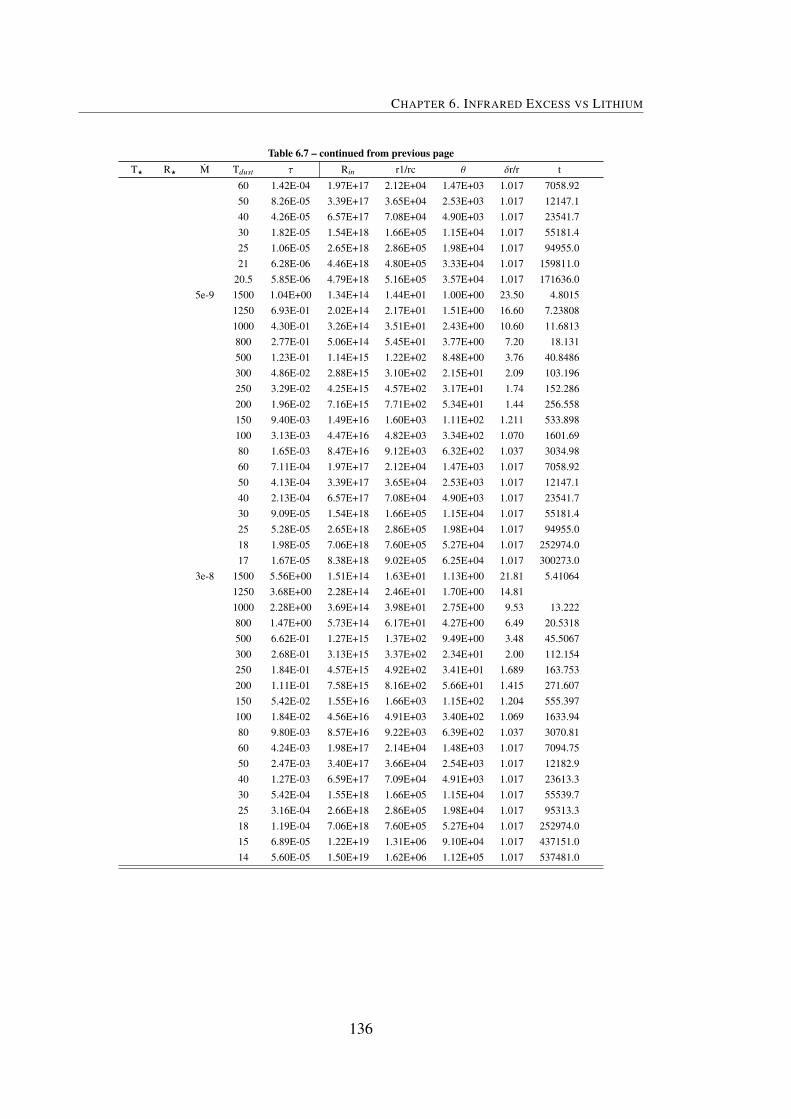
CHAPTER 6. INFRARED EXCESS VS LITHIUM
Table 6.7 – continued from previous pageT? R? M Tdust τ Rin r1/rc θ δr/r t
60 1.42E-04 1.97E+17 2.12E+04 1.47E+03 1.017 7058.9250 8.26E-05 3.39E+17 3.65E+04 2.53E+03 1.017 12147.140 4.26E-05 6.57E+17 7.08E+04 4.90E+03 1.017 23541.730 1.82E-05 1.54E+18 1.66E+05 1.15E+04 1.017 55181.425 1.06E-05 2.65E+18 2.86E+05 1.98E+04 1.017 94955.021 6.28E-06 4.46E+18 4.80E+05 3.33E+04 1.017 159811.0
20.5 5.85E-06 4.79E+18 5.16E+05 3.57E+04 1.017 171636.05e-9 1500 1.04E+00 1.34E+14 1.44E+01 1.00E+00 23.50 4.8015
1250 6.93E-01 2.02E+14 2.17E+01 1.51E+00 16.60 7.238081000 4.30E-01 3.26E+14 3.51E+01 2.43E+00 10.60 11.6813800 2.77E-01 5.06E+14 5.45E+01 3.77E+00 7.20 18.131500 1.23E-01 1.14E+15 1.22E+02 8.48E+00 3.76 40.8486300 4.86E-02 2.88E+15 3.10E+02 2.15E+01 2.09 103.196250 3.29E-02 4.25E+15 4.57E+02 3.17E+01 1.74 152.286200 1.96E-02 7.16E+15 7.71E+02 5.34E+01 1.44 256.558150 9.40E-03 1.49E+16 1.60E+03 1.11E+02 1.211 533.898100 3.13E-03 4.47E+16 4.82E+03 3.34E+02 1.070 1601.6980 1.65E-03 8.47E+16 9.12E+03 6.32E+02 1.037 3034.9860 7.11E-04 1.97E+17 2.12E+04 1.47E+03 1.017 7058.9250 4.13E-04 3.39E+17 3.65E+04 2.53E+03 1.017 12147.140 2.13E-04 6.57E+17 7.08E+04 4.90E+03 1.017 23541.730 9.09E-05 1.54E+18 1.66E+05 1.15E+04 1.017 55181.425 5.28E-05 2.65E+18 2.86E+05 1.98E+04 1.017 94955.018 1.98E-05 7.06E+18 7.60E+05 5.27E+04 1.017 252974.017 1.67E-05 8.38E+18 9.02E+05 6.25E+04 1.017 300273.0
3e-8 1500 5.56E+00 1.51E+14 1.63E+01 1.13E+00 21.81 5.410641250 3.68E+00 2.28E+14 2.46E+01 1.70E+00 14.811000 2.28E+00 3.69E+14 3.98E+01 2.75E+00 9.53 13.222800 1.47E+00 5.73E+14 6.17E+01 4.27E+00 6.49 20.5318500 6.62E-01 1.27E+15 1.37E+02 9.49E+00 3.48 45.5067300 2.68E-01 3.13E+15 3.37E+02 2.34E+01 2.00 112.154250 1.84E-01 4.57E+15 4.92E+02 3.41E+01 1.689 163.753200 1.11E-01 7.58E+15 8.16E+02 5.66E+01 1.415 271.607150 5.42E-02 1.55E+16 1.66E+03 1.15E+02 1.204 555.397100 1.84E-02 4.56E+16 4.91E+03 3.40E+02 1.069 1633.9480 9.80E-03 8.57E+16 9.22E+03 6.39E+02 1.037 3070.8160 4.24E-03 1.98E+17 2.14E+04 1.48E+03 1.017 7094.7550 2.47E-03 3.40E+17 3.66E+04 2.54E+03 1.017 12182.940 1.27E-03 6.59E+17 7.09E+04 4.91E+03 1.017 23613.330 5.42E-04 1.55E+18 1.66E+05 1.15E+04 1.017 55539.725 3.16E-04 2.66E+18 2.86E+05 1.98E+04 1.017 95313.318 1.19E-04 7.06E+18 7.60E+05 5.27E+04 1.017 252974.015 6.89E-05 1.22E+19 1.31E+06 9.10E+04 1.017 437151.014 5.60E-05 1.50E+19 1.62E+06 1.12E+05 1.017 537481.0
136

CHAPTER 7
ORIGIN OF LI ENHANCEMENT IN KGIANTS
The origin of Li anomaly in a small number of K giants are discussed here in the contextof two prominent suggestions given in literature, (i) external origin by engulfment ofplanets or brown dwarfs, (ii) internal synthesis of Li and associated mixing process. Inorder to understand these issues, we study the evolution of Li and infrared excess in largenumber of sample giants starting from the base to well beyond the post luminosity bumpin the H-R diagram.
In this chapter, we discuss the results from a large survey of K giants designed to findadditional Li-rich examples, locate their appearance in the HR diagram and so provideessential material for testing hypotheses about Li-enrichment. For example, Li produc-tion may be associated with the bump in the luminosity function for stars on the RGBas suggested from observations by Charbonnel & Balachandran (2000). Depending onmass and composition the bump occures on RGB between luminosities, log (L/L) = 1.5- 2.2, and this has been predicted (Iben 1968) as a region where evolution of a giant isslowed down creating a bump in the luminosity function of stars along the RGB. Inter-nally, the bump is associated with the H-burning shell crossing over of H-discontinuity.Additionally or alternatively, the He-core flash may be the trigger for Li production andthe creation of Li-rich red clump (horizontal branch) stars. Discrimination between bumpand clump is possible because the two groups appear in somewhat different places in theHR diagram. Our 2000 giants provide a reference sample comfortably spanning the lu-minosity of the clump and the bump. Also, the survey designed to test the suggestion ofplanet engulfment scenario by including giants from all the way from the base of RGBto well above the clump/bump luminosities. With Brown et al.’s survey, a total of 2644
137

CHAPTER 7. ORIGIN OF LI ENHANCEMENT IN K GIANTS
giants covering a wide range of luminosities and effective temperatures represent a potentdatabase in which to search for clues to the origin of the Li enrichment in K giants.
7.1 THE HERTZSPRUNG-RUSSELL DIAGRAM
7.1.1 SAMPLE GIANTS
The sample consists of 2000 giants from our survey and 644 giants from Brown’s survey(B89). Luminosity and temperature of B89 samples are rederived in the similar fashion toour survey samples that are described in the Chapter 3. The distribution of luminosity andtemperature of these samples are shown in Figure 7.1. Note the samples are peaking atluminosity around 1.7 - 1.8 , which is well a known clump luminosity. However, samplestars peak in temperature at two places; 4500 K and 4850 K, which corresponds to bumpand clump regions, respectively.
1 2 3 4Luminosity
0
200
400
600
800
No.
of G
iant
s
4000 4500 5000Temperature
0
100
200
300
400
No.
of G
iant
s
Figure 7.1: Distribution of samples from our survey and Brown et al.’s survey. Luminosi-ties are in left panel and Temperatures are in right panel.
The giants from our and B89 surveys are shown on the HR diagram in Figure 7.2 alongwith evolutionary tracks (Bertelli et al. 2008) computed for solar metallicity, [Fe/H] = 0.0,and stellar masses ranging from 0.8M to 3M. our sample, shown in blue symbols, oc-cupy from the base of RGB to post luminosity bump whereas B89 sample starts fromclump luminosity to well beyond the post-luminosity bump region. Combined samplefrom both the surveys covers from all the way from the base of RGB to well above thepost clump/bump luminosities in the H-R diagram. All stars observed at low resolutionare assumed to have solar metallicity. For Li-rich K giants and B89 sample actual metal-licities are available from the high resolution spectra and most of them are turned out to
138

7.1 THE HERTZSPRUNG-RUSSELL DIAGRAM
be close to solar values. Errors derived from the quoted uncertainties in the parallaxesand in the derivation of temperatures for the Li-rich K giants are marked in Figure 7.3
5500 5000 4500 4000
0.5
1
1.5
2
2.5
3
[Fe/H] = 0.0
5500 5000 4500 4000
0.5
1
1.5
2
2.5
3
[Fe/H] = 0.0
5500 5000 4500 4000
0.5
1
1.5
2
2.5
3
[Fe/H] = 0.0
5500 5000 4500 4000
0.5
1
1.5
2
2.5
3
[Fe/H] = 0.0
5500 5000 4500 4000
0.5
1
1.5
2
2.5
3
[Fe/H] = 0.0
Figure 7.2: Sample stars of our survey in blue symbols and from B89 survey in greensymbols are shown in the HR diagram. Evolutionary tracks of stars of masses from 0.8to 3.0M and of solar metallicity, [Fe/H]=0.0, computed by Bertelli et al. (2008) are alsoshown. The base of the RGB and the extent of RGB bump are marked as broken and solidred lines, respectively. The RGB clump region is shown as a thick yellow line.
Vast majority of stars in the two samples have evolved beyond the base of the RGB(the red dashed line in Figure 7.2) and, therefore, their surface Li abundance must havebeen greatly diluted. In Figure 7.2, there is the expected concentration of stars withluminosities of about log(L/L) ' 1.7. This population in the HR diagram are red clumpstars (horizontal branch) with He-core burning core that have evolved from the tip of theRGB: the thick black line in Figure 7.2 shows the predicted locations of clump stars.Extension of the log(L/L) ' 1.7 concentration to cooler temperatures may include starsat the bump luminosity of the first ascent RGB stars (see red portions of the evolutionarytracks). Dominance of the HR diagram by clump stars is expected because the lifetime
139

CHAPTER 7. ORIGIN OF LI ENHANCEMENT IN K GIANTS
of a clump star is typically one to two orders of magnitude longer than for a bump star.This argument is not strictly applicable to the Li-rich stars because their frequency is alsodependent on the probabilities that clump and bump stars produce lithium.
Except for five luminous examples, the Li-rich stars are either at the luminosity of theclump or within the range of expected values for the bump, a range spanning the clump’sluminosity. The five luminous exceptions must owe their Li richness to different phenom-ena than those accounting for the majority of the Li-rich stars. For example, HD 39853(Gratton & D’Antona 1989) in Figure 7.3 is a Li-rich K giant but with log(L/L) = 2.7 isprobably a post-clump early AGB candidate where, as discussed by Charbonnel & Bal-achandran (2000), Li-production by the Cameron-Fowler mechanism has occurred by avariant of its operation in bump stars (see below). In contrast, the high luminosity warm(Teff = 5150K) Li-rich star HD 21018 is, as suggested by Charbonnel & Balachandran(2000), caught prior to dilution of lithium by the convective envelope, i.e., it is a Li-normal star exhibiting a Li abundance close to its in initial abundance. We focus here onthe Li-rich giants at bump and clump luminosities.
7.2 LI-EXCESS IN K GIANTS
7.2.1 EXTERNAL ORIGIN AN UNLIKELY SCENARIO
The idea of a planet or a brown dwarf engulfment scenario for explaining the Li-excessin the K giants has been there for quite a long time (Alexander 1967; Brown et al. 1989).They argued that sufficient amount of earth-like planetary mass with devoid of H mayenhance the Li abundance to the observed levels. Recent findings of exo-solar planetarysystems of main sequence as well as giants, and in some cases planets orbiting closer tothe central star, further raised such a possibility. Siess & Livio (1999) , inspired by theserecent findings, computed the possible effects of such mergers on the RGB phase, andproposed that accretion of a planet or a brown dwarf is responsible for high Li enhance-ment in the envelops of K giants and also the mass loss. And to a certain extent highrotation observed among the Li-rich K giants was attributed to the imparting of angularmomentum to the K giants by the merger events (see also Carlberg et al. 2010). In therecent observational finding Carlberg et al. (2010) interprets the super Li-richness in aK giant G0928+73.2600 and its high rotation as due to the planet engulfment. Obser-vational studies of individual Li-rich candidates (Reddy et al. 2002; Drake et al. 2002;Reddy & Lambert 2005) explored the possibilities of planet engulfment scenarios to si-multaneously explain rotation, infrared excess and also high amount of Li.
140

7.2 LI-EXCESS IN K GIANTS
5500 5000 4500 4000
0.5
1
1.5
2
2.5
3
[Fe/H] = 0.0
5500 5000 4500 4000
0.5
1
1.5
2
2.5
3
[Fe/H] = 0.0
5500 5000 4500 4000
0.5
1
1.5
2
2.5
3
[Fe/H] = 0.0
5500 5000 4500 4000
0.5
1
1.5
2
2.5
3
[Fe/H] = 0.0
Figure 7.3: Same as Figure 7.2. New Li-rich giants are in blue symbols and green symbolsare from Brown and magenta symbols are other known Li-rich giants.
Siess & Livio (1999) engulfment model suggests accretion mass of more than 0.12M
is required to replenish Li to the observed level. To put this in perspective a K giantenvelope needs to be mixed-up with planetary material of mass more than 30,000 earth-like planets or 100 Jupiter-like planets. In case of brown dwarfs, one may require at least5 - 10 brown dwarfs as massive as 10 - 20 Jupiter masses. Engulfment of very massivebrown dwarfs won’t be helpful as Li gets destroyed due to higher central temperaturesand convection. It is not clear whether such events have to occur at once or in someintervals. Based on our current observational evidence shown in Figures 7.2 & 7.3 , weargue that the engulfment is very unlikely scenario. If planet engulfment is the reasoneither directly or indirectly to the Li enhancement, one may expect Li-rich K giants allalong the RGB phase. However, examination of the HR diagram, as shown in Figure 7.2,reveals otherwise. All of the Li-rich K giants in the mass range of 0.8 - 3.0M, withinuncertainties, occupy a narrow region on the HR diagram: 1.4 ≥ log(L/L) ≤ 2.2 and
141

CHAPTER 7. ORIGIN OF LI ENHANCEMENT IN K GIANTS
4300 ≥ Teff ≤ 5100 K. This narrow luminosity region is overlapped with bump and clumpwhich has an important consequence in our quest for searching clues for origin of excessLi in the K giants.
7.2.2 LITHIUM-SYNTHESIS AT THE BUMP AND/OR CLUMP?
Since the Li-rich K giants are concentrated within a narrow luminosity range, one maysuppose a significant event must be associated directly or indirectly with this range. Onesuspects that the significant event is either the bump on the first ascent of the RGB and/orassociated with the red clump formed of He-core burning giants that have experiencedthe He-core flash at the tip of the RGB.
The observed luminosity range is crossed by first ascent RGB stars in which the H-burning shell passes into the region that previously was the maximum extent reachedby the convective envelope. When the outward moving H-burning shell, as a result ofincreasing He-core mass, first encounters this region, a star reacts to the increased avail-ability of H by lowering the surface luminosity. After a while, the giant continues itsascent of the RGB. This creates a kink on the evolutionary tracks for stars of masses upto 2M (Iben 1968; Bertelli et al. 2008) and a bump in the luminosity function along theRGB. As shown in Figure 7.2, the kink on the evolutionary tracks (Bertelli et al. 2008) isvisible only up to 2M for solar metallicity stars.
Internally, the kink is associated with an inversion in the run of mean molecular weightwith distance from the stellar center. This inversion is linked to destruction of 3He by thereaction 3He(3He,2p)4He which lowers the mean molecular weight, and the homogeniza-tion of the composition within the convective enevelope. Eggleton et al. (2008) show thatthis inversion leads to ‘compulsory’ mixing and changes to the surface abundances ofC,N, and O isotopic abundances, i.e., the 12C/13C ratio is lowered relative to its value be-fore the bump. Charbonnel & Lagarde (2010) recognize too that mixing occurs as a resultof the molecular weight inversion but include the effects of rotationally-induced mixingto drive the mixing. This mixing referred to as δµ-mixing by Eggleton et al. (2008) orthermohaline mixing by Charbonnel & Lagarde (2010) is observationally confirmed bymeasurements of the 12C/13C ratio in giants along the RGB showing a decrease in theratio at and above the luminosity of the bump.
As p-captures on 12C create 13C, the reservoir of primordial and main-sequence syn-thesized 3He is depleted. It is this reservoir that is a potential source of 7Li from theCameron-Fowler (Cameron & Fowler 1971) mechanism (3He(4He,γ)7Be(e−, ν)7Li) but inorder for the 7Li to enrich the stellar atmosphere and its progenitor 7Be must be swept
142
7.2 LI-EXCESS IN K GIANTS
quickly to temperatures too cool for proton captures to occur. Eggleton et al. (2008) cal-culations show that more than about 80% of the 3He is destroyed in stars of masses lessthan about 1.5M. This destruction seems unlikely to produce lithium because the mix-ing is too slow for the 7Be and 7Li to avoid destruction by protons (Lattanzio et al. 2008).However, the initial subsurface 3He reservoir is such that only a minor fraction of the 3Heneed be converted with moderate efficiency to provide a Li-rich giant. It is anticipatedthat the lithium produced as the star crosses the bump’s luminosity may be destroyed asthe star with its convective envelope evolves to the tip of the RGB.
The evidence from Figure 7.3 is that few of the Li-rich stars are aligned along therun of bump stars in the HR diagram. Although the cooler Li-rich stars are likely to bebump stars, many Li-rich stars are too warm to be so identified. Thus, we suggest thatLi-rich stars cannot be identified exclusively with the bump. Rather the colocation of theLi-rich stars in Figure 7.3 with the high concentration of observed (Li-normal) giants andthe theoretical location of the clump suggests that they are clump stars. If Li producedat the bump on the RGB survives a star’s evolution from the bump to the clump, suchLi-rich stars may appear predominantly as clump stars because the lifetime at the clumpis similar to or longer than the time to evolve through the bump and to the clump via thetip of the RGB. Since Li, if produced at the bump on the RGB, may be destroyed by thetime the star has evolved up the RGB to experience the He-core flash, the speculationis that the Cameron-Fowler mechanism may also operate at the He-core flash in at leastsome stars, i.e.,in stars of M < 2.25M. Since Eggleton et al. (2008) predict survival of3He in stars with M > 1.5M, there seems in principal the possibility that the He-coreflash may be the key to synthesis of lithium in stars in a narrow mass range centered atabout 2M with the range’s the upper limit set by the maximum mass for a He-core flashand the lower limit set by survival of sufficient 3He following δµ or thermohaline mixingon the RGB. Evidently, the concentration of Li-rich stars at the clump implies that thesynthesized Li is swiftly destroyed as a clump star evolves along the early reaches of theAGB. If all stars evolving through the He-core flash synthesize copious amounts of Li,they survive as a Li-rich giant for about one per cent of their horizontal branch lifetime,i.e., about 2 Myr. (The four luminous Li-rich stars in Figure 7.3 have a mass in excessof those experiencing the He-core flash. Charbonnel & Balachandran (2000) suggest thatthese tap their 3He to produce Li as the He-burning shell evolves outward.)
143

CHAPTER 7. ORIGIN OF LI ENHANCEMENT IN K GIANTS
7.3 BUMP AND CLUMP
To understand the Li-rich association with bump and/or clump, we studied the infraredproperties of Li-rich giants and giants without Li from bump and clump region in theHR-diagram. The infrared study of these sample stars suggested that mass-loss rates arehigher for Li-rich giants compare to normal giants. Li-rich stars on theoretical IRAScolor-color diagram revealed that Li-rich bump stars are associated with slightly warmerdust shells compare to Li-rich clump stars. The location of Li-rich giants in the IRASdiagram and the relation obtained between mass-loss rates and Li abundances suggestedthat Li timescales are in the order of 103 to 105 years.
Li timescales compared with the timescales of bump, clump and bump to clump,given in Table 6.6, suggested that Li timescales are less than bump timescales (≈106),clump timescales (≈107), evolutionary timescales from RGB tip to clump (≈106), andevolutionary timescales from bump to clump (≈107).
As the dust evolutionary timescles are comparable to Li timescales and are lessercompare to the timescales of a star that travel from bump to clump, which are in theorder of ten million years for stellar masses above 2 M, it is impossible to see the dustaround clump stars that is surviving from the bump and hence Li produced at bump cannot survives to clump. In this case, the dust around clump stars may be due to their strongstellar winds or mass-loss occurs due to the structural changes during He core flash atRGB tip. However, the mass-loss at He-core flash at RGB tip is neglected because theenormous amount of energy releases at the time of flash wont reach to the surface. Incase the dust forms at RGB tip, shell evolutionary timescales must be higher than thetimescales of a star to settle in red clump from the RGB tip, to see the signatures of thedust around clump stars. The proportion of Li-rich clump stars should be equal to thestars associated with the circumstellar dust at clump, to relate the Li enhancement withmassloss at core He flash.
7.4 CONCLUSIONS
The principal novel result here is that the majority of Li-rich K giants have a luminosityand effective temperature combination suggesting that Li production may occur at theHe-core flash in those stars. Although this speculation about the He-core flash has yet tobe supported by calculations, the nuclear physics of Li production is surely that describedby the Cameron-Fowler mechanism, i.e., conversion of 3He to 7Li by α-capture with7Be as a radioactive intermediary. An earlier suggestion that Li production, also by the
144

7.4 CONCLUSIONS
Cameron-Fowler mechanism, occurs at the luminosity bump of the RGB (Charbonnel& Balachandran 2000) is required to account for cooler Li-rich stars but may, if the Liproduced at the bump survives evolution from there to the clump, account for some or allof the Li-rich clump stars. Infrared study of Li-rich giants suggesting that Li producedat the bump can not survives to clump, therfore, high Li seen in clump stars may beaccounted for production of Li during He-core flash. Our discovery of that Li-rich giantsare concentrated within a narrow luminosity range does not support a view that Li-richgiants result from the swallowing by the giant of a gaseous planet (Alexander 1967) orsome other external origin.
145


CHAPTER 8
CONCLUSIONS AND FUTURE WORK
8.1 SUMMARY OF RESULTS
In this study we dealt with the long standing problem of unexpectedly high amount of Liin K giants. This was done in three parts. In part one we made a comprehensive surveyfor Li-rich K giants among K giants using low resolution spectroscopy. A sample of2000 K giants of brightness and volume limited were chosen from the Hipparcos catalogwhich contains one hundred thousand stars with accurate astrometry. Sample was chosenin such a way that it covers the RGB all the way from the base of RGB to well abovethe luminosity bump in the HR diagram. Entire low resolution spectra were obtainedwith the IIA facilities located at Vainu Bappu Observatory (VBO), Kavalur and IndianAstronomical Observatory, Hanle, Ladak. Telescopes used were 1-m CZT and 2.3-mVBT at VBO and 2.3-m HCT at IAO. We note that this is the largest survey of its kindin the literature. Observations were carried over the period of three years from 2006 to2009. Spectra were analyzed for finding Li enhanced K giants. In the phase I of our studywe measured core strengths of Li resonance line at 6707.7 Å and the nearby Ca I line at6717.6 Å. For given metallicity and Teff , the ratio of Li line to Ca I line would indicatethe level of Li enhancement in a given star. An empirical relation between the actual Limeasured from high resolution and the ratio of line strengths from low resolution spectrawas derived. In deriving the relation, we used number of known Li-rich K giants as wellas normal K giants. This way, we found 15 Li-rich K giant candidates . Some are superLi-rich. Also, the survey confirmed the rarity of Li-rich K giants i.e., 1% among the Kgiants in the Galaxy.
In the second part of this study, we focused on the high resolution spectroscopic studyof the new and old Li-rich K giants. We have performed spectral analysis to derive quan-
147

CHAPTER 8. CONCLUSIONS AND FUTURE WORK
titative abundances of Li, C, N, and O and carbon isotopic ratio 12C/13C. With the highresolution spectroscopy, we have confirmed all the 15 Li-rich giant candidates as Li-richK giants. Four among them are super Li-rich with log ε (Li) ≥ 3.3 dex, about a factor of100 more than the expected Li in K giants. The current study resulted in highest numberof K giants in any one single study. With this findings, the total number of Li-rich Kgiants in the literature went up by a factor of two. The total number of super Li-rich Kgiants to twelve. The study also threw-up some new interesting results. Three Li-richK giants are found to have anomalous low 12C/13C, very close to CN equilibrium value.Such low values are expected very close to the RGB tip or in the very metal-poor stars.It is puzzling that such low values are found to be at the RGB bump in solar metallicitystars and they are super Li-rich and this suggests severe mixing process must be somehowrelated to Li enhancement.
Results show that all the Li-rich K giants lie in a narrow luminosity range of log(L/L) = 1.4 - 2.2 spanning in Teff = 4300 - 5100 K. The region overlaps with the lu-minosity bump and also the red clump region in the HR diagram. However, no Li-richgiants were found either too below the luminosity bump or too above the bump. This is animportant result which rules out the frequent suggestions of planet engulfment scenariofor the Li enrichment in K giants. Since the bump region is associated with importantstructural changes in the interior, we suggest that somehow this is linked to the high Li.Absence of high Li before or after the bump indicates that Li phenomenon in giants isvery short, and, utmost, it lasts for the duration of the bump evolution. This is estimatedfrom the evolutionary tracks as few thousand years depending on mass. Amount of Liin super-Li rich stars clearly rules out the earlier suggestion of preservation of main se-quence Li. From this study we reinforce ideas of internal nucleosynthesis for Li-origin inK giants.
We have searched for clues for Li origin question in terms of Li enhancement patternswith other elemental abundances which are sensitive to mixing on RGB. Abundancesof C and N in all of the Li-rich giants follow the theoretical predictions i.e., carbon ismodestly depleted and N is modestly enhanced. These are the byproducts of CN cyclein H-burning cycle. However, O remained constant as ON cycle requires much highercentral temperatures. However, HD 12203 is an exception for its C, N, and O abundanceswhich are significantly different from the rest of Li-rich K giants. It’s kinematics showthat the star is a member of Galactic thick disk, and all others are thin disk members. ItsC and N abundances are attributed to either its mass or its status as early AGB stars. Thedecrease in C and increase in N abundances show no dependency with the Li enhancement
148

8.1 SUMMARY OF RESULTS
in K giants. The 12C/13C ratios show some interesting results. The 12C/13C ratios of thecombined sample do not indicate correlation with Li abundance in K giants. However, thenew sample of K giants do show a correlation between 12C/13C and Li. The K giants thathave lower 12C/13C values have much higher Li abundances. This is a surprising resultwhich suggests some sort of extra mixing that is responsible for reducing 12C/13C andenhancing Li abundance.
Another aspect of K giants is the rotation. Rotational velocities for all the Li-rich Kgiants were obtained. Results indicate that there is no particular trend of high rotationwith high Li. There are just six Li-rich giants (out of total 24 that are known) whichshow anomalous high rotation (≥ 8 km s−1). From the current results we suggest thathaving slightly higher rotation among a small fraction of K giants is normal. In fact, thisparticular result is drawn from our study of rotational velocity distribution among dwarfsand giants (this study is not included in the thesis).
In the third part of this thesis we dealt with infrared excess and the Li abundances.The study does not throw any definite results related to our quest for Li origin. However,we found K giants that are at the bump showing higher mass loss rates and warmer dusttemperatures relative to other regions such as clump and pre-bump regions. This meansthat recent mass loss occurrence at the bump. Whether this is related to the Li enrichmentis an important question. Also, modeling of dust shells using DUSTY suggests that theLi-rich K giants have non-spherical dust shells with truncated polar caps, and the normalK giants have spherical dust shells. Again, these results hint likely association of massejections at the bump with Li enhancement.
8.1.1 IMPACT OF THIS STUDY
The principal results that will impact the field in this particular area are:
• Finding of large number of Li-rich K giants includes four super Li-rich K giants.With this study total number of Li-rich K giants went up by a factor of two i.e.about 25 and the number of super-Li rich K giants went up to 12. These resultssignificantly improved the statistical significance of the sample and interpretationof their properties
• Fractional content of Li-rich K giants are ≤ 1% among K giants in the Galaxy froman unbiased survey of brightness and volume limited sample
• Another important result is finding of very low 12C/13C values among three super
149
CHAPTER 8. CONCLUSIONS AND FUTURE WORK
Li-rich K giants. Results of C,N, O and 12C/13C for a full set of Li-rich K giantsand their trends with Li would help to constrain theoretical modeling
• Results suggest that high rotational property of the Li-rich K giants seems to becoincidental and is also seen among normal K giants
8.2 FUTURE PLANS
Several interesting issues came to light in this study. For example it is not very clearhow the Li-rich K giants are distributed, in the HR diagram, among the clump and/orbump regions. In our study, almost 50% of K giants occupy the bump regions and therest occupy a region called the red clump. Giants at the red clump are the ones thathave evolved off the RGB tip. On the other hand, stars at the bump are climbing theRGB for the first time towards RGB tip. Discrimination of these regions would help inidentifying the physical process that are associated with Li-rich K giants. Unambiguousidentification is quite difficult among field RGB stars. However, this could be achievedin clusters where the bump and clump regions are well defined and separated from eachother. Globular clusters are ideal for such studies. However, stars in the globular clustersare quite faint, and requires 8 - 10-m class telescopes with multi-object spectrographs andthis will be investigated at a later point of time.
Another important aspect that we could right away initiate is that variability study ofLi-rich K giants. It is not clear whether binarity is some how related to the Li-richness.Though such a possibility is remote, given the results in this study, it would be an im-portant exercise to take up 2 to 3 years of continuous monitoring of all the Li-rich Kgiants and eliminate that possibility. As of now, no such studies are initiated, as they needmodest size telescopes.
In this study we mostly concentrated on extracting results from observations and in-terpreting them with the help of standard stellar mixing theory and the recently developedextra mixing models of RGB stars. One of the bigger pictures that we had envisaged atthe time of embarking on the survey was to estimate RGB stars contribution to the totalLi in the Galaxy. This would have put some real constraints on the Li evolution in theGalaxy. We are hoping to carry out such studies in due course of time.
150
REFERENCES
Alexander, J. B. 1967, The Observatory, 87, 238
Allende Prieto, C., Asplund, M., Lopez, R. J. G., & Lambert, D. L. 2002, ApJ, 567, 544
Allende Prieto, C., Lambert, D. L., & Asplund, M. 2001, ApJ, 556, L63
Alonso, A., Arribas, S., & Martınez-Roger, C. 1999, A&AS, 140, 261
Andrievsky, S. M., Gorlova, N. I., Klochkova, V. G., Kovtyukh, V. V., & Panchuk, V. E.1999, Astronomische Nachrichten, 320, 35
Aoki, W., Barklem, P. S., Beers, T. C., et al. 2009, ApJ, 698, 1803
Arnould, M. & Norgaard, H. 1975, A&A, 42, 55
Asplund, M., Lambert, D. L., Nissen, P. E., Primas, F., & Smith, V. V. 2006, ApJ, 644,229
Balachandran, S. C., Fekel, F. C., Henry, G. W., & Uitenbroek, H. 2000, ApJ, 542, 978
Bellazzini, M., Gennari, N., & Ferraro, F. R. 2005, MNRAS, 360, 185
Belyaev, A. K. & Barklem, P. S. 2003, Phys. Rev. A, 68, 062703
Bertelli, G., Girardi, L., Marigo, P., & Nasi, E. 2008, A&A, 484, 815
Bidelman, W. P. 1951, ApJ, 113, 304
Biemont, E., Hibbert, A., Godefroid, M., & Vaeck, N. 1993, ApJ, 412, 431
Boesgaard, A. M. 1970, ApJ, 161, 1003
Boesgaard, A. M. & Tripicco, M. J. 1986, ApJ, 302, L49
Bonifacio, P., Molaro, P., Sivarani, T., et al. 2007, A&A, 462, 851
Bonifacio, P., Pasquini, L., Spite, F., et al. 2002, A&A, 390, 91
Boothroyd, A. I. & Sackmann, I.-J. 1999, ApJ, 510, 232
Brown, J. A., Sneden, C., Lambert, D. L., & Dutchover, E. J. 1989, ApJS, 71, 293
151

REFERENCES
Cameron, A. G. W. & Fowler, W. A. 1971, ApJ, 164, 111
Carlberg, J. K., Smith, V. V., Cunha, K., Majewski, S. R., & Rood, R. T. 2010, ApJ, 723,L103
Carlsson, M. 1986, Uppsala Astronomical Observatory Reports, 33
Carlsson, M. 1992, in Astronomical Society of the Pacific Conference Series, Vol. 26,Cool Stars, Stellar Systems, and the Sun, ed. M. S. Giampapa & J. A. Bookbinder,499–+
Carlsson, M., Rutten, R. J., Bruls, J. H. M. J., & Shchukina, N. G. 1994, A&A, 288, 860
Carpenter, J. M. 2001, AJ, 121, 2851
Castelli, F., Gratton, R. G., & Kurucz, R. L. 1997a, A&A, 324, 432
Castelli, F., Gratton, R. G., & Kurucz, R. L. 1997b, A&A, 318, 841
Castelli, F. & Hack, M. 1990, Mem. Soc. Astron. Italiana, 61, 595
Castilho, B. V., Gregorio-Hetem, J., Spite, F., Spite, M., & Barbuy, B. 1998, A&AS, 127,139
Charbonnel, C. 1995, ApJ, 453, L41+
Charbonnel, C. & Balachandran, S. C. 2000, A&A, 359, 563
Charbonnel, C., Brown, J. A., & Wallerstein, G. 1998, A&A, 332, 204
Charbonnel, C. & Lagarde, N. 2010, ArXiv e-prints
Clarke, D. 1964, The Observatory, 84, 28
Cottrell, P. L. & Norris, J. 1978, ApJ, 221, 893
Cox, A. N. 2000, Allen’s astrophysical quantities, ed. Cox, A. N.
Croft, H., Dickinson, A. S., & Gadea, F. X. 1999, MNRAS, 304, 327
Cutri, R. M., Skrutskie, M. F., van Dyk, S., et al. 2003, 2MASS All Sky Catalog of pointsources., ed. Cutri, R. M., Skrutskie, M. F., van Dyk, S., Beichman, C. A., Carpenter,J. M., Chester, T., Cambresy, L., Evans, T., Fowler, J., Gizis, J., Howard, E., Huchra,J., Jarrett, T., Kopan, E. L., Kirkpatrick, J. D., Light, R. M., Marsh, K. A., McCallon,H., Schneider, S., Stiening, R., Sykes, M., Weinberg, M., Wheaton, W. A., Wheelock,S., & Zacarias, N.
Cyburt, R. H., Fields, B. D., & Olive, K. A. 2008, J. Cosmology Astropart. Phys., 11, 12
D’Antona, F. & Matteucci, F. 1991, A&A, 248, 62
152

REFERENCES
Dantona, F. & Mazzitelli, I. 1982, ApJ, 260, 722
de La Reza, R. & da Silva, L. 1995, ApJ, 439, 917
de La Reza, R., Drake, N. A., & da Silva, L. 1996, ApJ, 456, L115+
de La Reza, R., Drake, N. A., da Silva, L., Torres, C. A. O., & Martin, E. L. 1997, ApJ,482, L77+
de Laverny, P. & Gustafsson, B. 1998, A&A, 332, 661
De Medeiros, J. R., do Nascimento, Jr., J. D., Sankarankutty, S., Costa, J. M., & Maia,M. R. G. 2000, A&A, 363, 239
de Medeiros, J. R., Melo, C. H. F., & Mayor, M. 1996, A&A, 309, 465
Dehnen, W. & Binney, J. J. 1998, MNRAS, 298, 387
Della Valle, M., Pasquini, L., Daou, D., & Williams, R. E. 2002, A&A, 390, 155
Denissenkov, P. A. & Herwig, F. 2004, ApJ, 612, 1081
Denissenkov, P. A. & Weiss, A. 2000, A&A, 358, L49
Di Cecco, A., Bono, G., Stetson, P. B., et al. 2010, ApJ, 712, 527
Diaz-Cordoves, J., Claret, A., & Gimenez, A. 1995, A&AS, 110, 329
Domınguez, I., Abia, C., Straniero, O., Cristallo, S., & Pavlenko, Y. V. 2004, A&A, 422,1045
Drake, N. A., de la Reza, R., da Silva, L., & Lambert, D. L. 2002, AJ, 123, 2703
Dunkley, J., Komatsu, E., Nolta, M. R., et al. 2009, ApJS, 180, 306
Eggleton, P. P., Dearborn, D. S. P., & Lattanzio, J. C. 2008, ApJ, 677, 581
Fekel, F. C. 1997, PASP, 109, 514
Fekel, F. C. & Marschall, L. A. 1991, AJ, 102, 1439
Fekel, F. C. & Watson, L. C. 1998, AJ, 116, 2466
Frankowski, A., Jancart, S., & Jorissen, A. 2007, A&A, 464, 377
Fuhr, J. R. & Wiese, W. L. 2006, Journal of Physical and Chemical Reference Data, 35,1669
Gilroy, K. K. 1989, ApJ, 347, 835
Girardi, L., Bressan, A., Bertelli, G., & Chiosi, C. 2000, A&AS, 141, 371
153

REFERENCES
Gonzalez, O. A., Zoccali, M., Monaco, L., et al. 2009, A&A, 508, 289
Gratton, R. G., Bragaglia, A., Carretta, E., et al. 2003, A&A, 408, 529
Gratton, R. G. & D’Antona, F. 1989, A&A, 215, 66
Gratton, R. G., Sneden, C., Carretta, E., & Bragaglia, A. 2000, A&A, 354, 169
Gray, D. F. 1992, The observation and analysis of stellar photospheres., ed. Gray, D. F.
Gregorio-Hetem, J., Castilho, B. V., & Barbuy, B. 1993, A&A, 268, L25+
Guillout, P., Klutsch, A., Frasca, A., et al. 2009, A&A, 504, 829
Gustafsson, B., Karlsson, T., Olsson, E., Edvardsson, B., & Ryde, N. 1999, A&A, 342,426
Haakonsen, C. B. & Rutledge, R. E. 2009, ApJS, 184, 138
Hanni, L. 1984, Soviet Astronomy Letters, 10, 51
Harris, M. J., Lambert, D. L., & Smith, V. V. 1988, ApJ, 325, 768
Hartoog, M. R., Persson, S. E., & Aaronson, M. 1977, PASP, 89, 660
Hauck, B. & Mermilliod, M. 1998, A&AS, 129, 431
Hekker, S. & Melendez, J. 2007, A&A, 475, 1003
Hernanz, M., Jose, J., Coc, A., & Isern, J. 1996, ApJ, 465, L27+
Herwig, F. 2005, ARA&A, 43, 435
Hill, V. & Pasquini, L. 1999, A&A, 348, L21
Hinkle, K., Wallace, L., Valenti, J., & Harmer, D. 2000, Visible and Near Infrared Atlasof the Arcturus Spectrum 3727-9300 A, ed. Hinkle, K., Wallace, L., Valenti, J., &Harmer, D.
Hobbs, L. M., Thorburn, J. A., & Rebull, L. M. 1999, ApJ, 523, 797
Hosford, A., Ryan, S. G., Garcıa Perez, A. E., Norris, J. E., & Olive, K. A. 2009, A&A,493, 601
Houdashelt, M. L., Bell, R. A., & Sweigart, A. V. 2000, AJ, 119, 1448
Houk, N. 1982, Michigan Catalogue of Two-dimensional Spectral Types for the HD stars.Volume 3. Declinations -40 to -26., ed. Houk, N.
Hoyle, F. & Schwarzschild, M. 1955, ApJS, 2, 1
Iben, I. 1968, Nature, 220, 143
154

REFERENCES
Iben, Jr., I. 1973, ApJ, 185, 209
Iben, Jr., I. & Renzini, A. 1983, ARA&A, 21, 271
Iben, I. J. 1967a, ApJ, 147, 650
Iben, I. J. 1967b, ApJ, 147, 624
Ivezic, Z., Nenkova, M., & Elitzur, M. 1999, ArXiv Astrophysics e-prints
Jasniewicz, G., Parthasarathy, M., de Laverny, P., & Thevenin, F. 1999, A&A, 342, 831
Jeans, J. H. 1928, Astronomy and cosmogony, ed. Jeans, J. H.
Jose, J. & Hernanz, M. 1998, ApJ, 494, 680
Jura, M. 2003, ApJ, 582, 1032
Jura, M., Bohac, C. J., Sargent, B., et al. 2006, ApJ, 637, L45
Keenan, P. C. 1967, AJ, 72, 808
Kirkman, D., Tytler, D., Suzuki, N., O’Meara, J. M., & Lubin, D. 2003, ApJS, 149, 1
Knauth, D. C., Federman, S. R., & Lambert, D. L. 2003, ApJ, 586, 268
Knauth, D. C., Federman, S. R., Lambert, D. L., & Crane, P. 2000, Nature, 405, 656
Koen, C. & Eyer, L. 2002, MNRAS, 331, 45
Koornneef, J. 1983, A&A, 128, 84
Korn, A. J., Grundahl, F., Richard, O., et al. 2006, Nature, 442, 657
Kraft, R. P., Peterson, R. C., Guhathakurta, P., et al. 1999, ApJ, 518, L53
Kumar, Y. B. & Reddy, B. E. 2009, ApJ, 703, L46
Kurucz, R. L. 1970, SAO Special Report, 309
Kurucz, R. L. 1993, in Astronomical Society of the Pacific Conference Series, Vol. 44,IAU Colloq. 138: Peculiar versus Normal Phenomena in A-type and Related Stars, ed.M. M. Dworetsky, F. Castelli, & R. Faraggiana, 87–+
Kurucz, R. L. 1994, www.kurucz.harvard.edu
Kurucz, R. L. & Bell, B. 1995, Atomic line list, ed. Kurucz, R. L. & Bell, B.
Lambert, D. L. 1994, in Lecture Notes in Physics, Berlin Springer Verlag, Vol. 428, IAUColloq. 146: Molecules in the Stellar Environment, ed. U. G. Jorgensen, 1–+
Lambert, D. L., Dominy, J. F., & Sivertsen, S. 1980, ApJ, 235, 114
155
REFERENCES
Lambert, D. L. & Reddy, B. E. 2004, MNRAS, 349, 757
Lambert, D. L. & Sawyer, S. R. 1984, ApJ, 283, 192
Lattanzio, J. C., Dearborn, D. S. P., & Eggleton, P. P. 2008, in American Institute ofPhysics Conference Series, Vol. 1001, Evolution and Nucleosynthesis in AGB Stars,ed. R. Guandalini, S. Palmerini, & M. Busso, 279–286
Lemoine, M., Vangioni-Flam, E., & Casse, M. 1998, ApJ, 499, 735
Lind, K., Asplund, M., & Barklem, P. S. 2009, A&A, 503, 541
Lodders, K. 2003, ApJ, 591, 1220
Luck, R. E. 1982, PASP, 94, 811
Luck, R. E. & Heiter, U. 2007, AJ, 133, 2464
Luck, R. E. & Lambert, D. L. 1992, ApJS, 79, 303
Lynden-Bell, D. & Pringle, J. E. 1974, MNRAS, 168, 603
Maggio, A., Vaiana, G. S., Haisch, B. M., et al. 1990, ApJ, 348, 253
Makarov, V. V. & Kaplan, G. H. 2005, AJ, 129, 2420
Mallik, S. V. 1999, A&A, 352, 495
Matteucci, F. 2010, in IAU Symposium, Vol. 268, IAU Symposium, ed. C. Charbonnel,M. Tosi, F. Primas, & C. Chiappini, 453–461
McClure, R. D. & Forrester, W. T. 1981, Publications of the Dominion AstrophysicalObservatory Victoria, 15, 439
Meneguzzi, M., Audouze, J., & Reeves, H. 1971, A&A, 15, 337
Mishenina, T. V., Bienayme, O., Gorbaneva, T. I., et al. 2006, A&A, 456, 1109
Mishenina, T. V., Soubiran, C., Kovtyukh, V. V., & Belik, S. I. 2010, in IAU Symposium,Vol. 268, IAU Symposium, ed. C. Charbonnel, M. Tosi, F. Primas, & C. Chiappini,343–344
Mohler, S. 2004, in IAU Symposium, Vol. 224, The A-Star Puzzle, ed. J. Zverko,J. Ziznovsky, S. J. Adelman, & W. W. Weiss, 395–402
Monaco, L. & Bonifacio, P. 2008, Mem. Soc. Astron. Italiana, 79, 524
Monaco, L., Villanova, S., Moni Bidin, C., et al. 2011, ArXiv e-prints
Monet, D. G., Levine, S. E., Canzian, B., et al. 2003, AJ, 125, 984
156

REFERENCES
Muthumariappan, C., Kwok, S., & Volk, K. 2006, ApJ, 640, 353
Olive, K. A. & Schramm, D. N. 1992, Nature, 360, 439
Ossenkopf, V., Henning, T., & Mathis, J. S. 1992, A&A, 261, 567
Pakhomov, Y. V., Antipova, L. I., & Boyarchuk, A. A. 2011, Astronomy Reports, 55, 256
Palacios, A., Charbonnel, C., & Forestini, M. 2001, A&A, 375, L9
Palacios, A., Charbonnel, C., Talon, S., & Siess, L. 2006, A&A, 453, 261
Pallavicini, R., Spano, P., Prisinzano, L., Randich, S., & Sestito, P. 2006, Multi-ObjectSpectroscopy of Open Clusters with FLAMES: Preliminary GTO Results, ed. Randich,S. & Pasquini, L., 181–+
Parthasarathy, M. & Rao, N. K. 1980, Ap&SS, 73, 251
Pavlenko, Y. V. & Magazzu, A. 1996, A&A, 311, 961
Perryman, M. A. C., Lindegren, L., Kovalevsky, J., et al. 1997, A&A, 323, L49
Piau, L., Beers, T. C., Balsara, D. S., et al. 2006, ApJ, 653, 300
Pilachowski, C. 1986, ApJ, 300, 289
Pilachowski, C., Saha, A., & Hobbs, L. M. 1988, PASP, 100, 474
Plez, B., Smith, V. V., & Lambert, D. L. 1993, ApJ, 418, 812
Prabhu, T. P., Anupama, G. C., & Surendiranath, R. 1998, Bulletin of the AstronomicalSociety of India, 26, 383
Randich, S., Bragaglia, A., Pastori, L., et al. 2005, The Messenger, 121, 18
Randich, S., Pallavicini, R., Meola, G., Stauffer, J. R., & Balachandran, S. C. 2001, A&A,372, 862
Rao, N. K. 1978, MNRAS, 185, 585
Rao, N. K., Sriram, S., Jayakumar, K., & Gabriel, F. 2005, JApA, 26, 331
Reddy, B. E. & Lambert, D. L. 2005, AJ, 129, 2831
Reddy, B. E., Lambert, D. L., & Allende Prieto, C. 2006, MNRAS, 367, 1329
Reddy, B. E., Lambert, D. L., Hrivnak, B. J., & Bakker, E. J. 2002, AJ, 123, 1993
Reddy, B. E., Tomkin, J., Lambert, D. L., & Allende Prieto, C. 2003, MNRAS, 340, 304
Reeves, H. 1970, Nature, 226, 727
157
REFERENCES
Richard, O., Michaud, G., & Richer, J. 2005, ApJ, 619, 538
Romano, D., Matteucci, F., Ventura, P., & D’Antona, F. 2001, A&A, 374, 646
Ryan, S. G., Beers, T. C., Olive, K. A., Fields, B. D., & Norris, J. E. 2000, ApJ, 530, L57
Sackmann, I. & Boothroyd, A. I. 1992, ApJ, 392, L71
Sackmann, I.-J. & Boothroyd, A. I. 1999, ApJ, 510, 217
Sackmann, I.-J., Smith, R. L., & Despain, K. H. 1974, ApJ, 187, 555
Salaris, M., Cassisi, S., & Weiss, A. 2002, PASP, 114, 375
Sato, B., Omiya, M., Liu, Y., et al. 2010, PASJ, 62, 1063
Scalo, J. M., Despain, K. H., & Ulrich, R. K. 1975, ApJ, 196, 805
Schild, R. E. 1973, AJ, 78, 37
Schroder, K. & Cuntz, M. 2005, ApJ, 630, L73
Sestito, P. & Randich, S. 2005, A&A, 442, 615
Siess, L. & Livio, M. 1999, MNRAS, 308, 1133
Smith, V. V. & Lambert, D. L. 1989, ApJ, 345, L75
Smith, V. V. & Lambert, D. L. 1990, ApJ, 361, L69
Smith, V. V., Lambert, D. L., & Nissen, P. E. 1993, ApJ, 408, 262
Smith, V. V., Lambert, D. L., & Nissen, P. E. 1998, ApJ, 506, 405
Smith, V. V., Plez, B., Lambert, D. L., & Lubowich, D. A. 1995, ApJ, 441, 735
Sneden, C., Lambert, D. L., Tomkin, J., & Peterson, R. C. 1978, ApJ, 222, 585
Sneden, C. & Pilachowski, C. A. 1984, PASP, 96, 38
Sneden, C. A. 1973, PhD thesis, AA(The University Of Texas at Austin.)
Spite, F. & Spite, M. 1982, A&A, 115, 357
Starrfield, S., Truran, J. W., Sparks, W. M., & Arnould, M. 1978, ApJ, 222, 600
Surendiranath, R., Vivekananda Rao, P., & Sarma, M. B. K. 1978, Acta Astron., 28, 231
Sweigart, A. V. & Mengel, J. G. 1979, ApJ, 229, 624
Takeda, Y. & Kawanomoto, S. 2005, PASJ, 57, 45
Torres-Peimbert, S. & Wallerstein, G. 1966, ApJ, 146, 724
158

REFERENCES
Travaglio, C., Randich, S., Galli, D., et al. 2001, ApJ, 559, 909
Tull, R. G., MacQueen, P. J., Sneden, C., & Lambert, D. L. 1995, PASP, 107, 251
van Leeuwen, F., ed. 2007, Astrophysics and Space Science Library, Vol. 350, Hipparcos,the New Reduction of the Raw Data
Voges, W., Aschenbach, B., Boller, T., et al. 1999, A&A, 349, 389
Wallerstein, G. & Morell, O. 1994, A&A, 281, L37
Wallerstein, G. & Sneden, C. 1982, ApJ, 255, 577
Woosley, S. E., Hartmann, D. H., Hoffman, R. D., & Haxton, W. C. 1990, ApJ, 356, 272
Woosley, S. E. & Weaver, T. A. 1995, ApJS, 101, 181
Yi, S. K., Kim, Y.-C., & Demarque, P. 2003, ApJS, 144, 259
Zuckerman, B., Kim, S. S., & Liu, T. 1995, ApJ, 446, L79+
159
